estimating the latent time of fault detection in finite automaton tested in real time

ISSN 0005-1179, Automation and Remote Control, 2008, Vol. 69, No. 10, pp. 1765–1777. c© Pleiades Publishing, Ltd., 2008.Original Russian Text c© R. Goot, I. Levin, 2008, published in Avtomatika i Telemekhanika, 2008, No. 10, pp. 128–141.

TECHNICAL DIAGNOSTICS

Estimating the Latent Time of Fault Detection

in Finite Automaton Tested in Real Time

R. Goot∗ and I. Levin∗∗∗Haifa Institute of Technology, Haifa, Israel

∗∗Tel Aviv University, Tel Aviv, IsraelReceived October 10, 2006

Abstract—The notions of potential and real latent times of fault detection in finite automatawere introduced. The potential latent time is the minimal theoretical time of automaton faultdetection, the real time is defined as the time of fault manifestation at a certain point. A methodfor determination of the statistical characteristics of both times for the automaton tested inthe course of its real operation was proposed. It is based on selection of the trajectories of theMarkov chain describing behavior of the operable and faulty automata. Additionally, a methodfor determination of the upper bound of the mean latent time in the case of limited informationabout the automaton characteristics was proposed.

PACS number: 89.20.Ff

DOI: 10.1134/S000511790810010X

1. INTRODUCTION

Digital system controllers usually are the most critical units in terms of checking and testing.Design of self-testing controllers and analysis of their efficiency is a challenge due, on the one hand,to their complexity and, on the other hand, to the key role they play in the system [1]. Thepresent paper considers the statistical characteristics of the latent time of fault detection for finiteautomata-controllers tested in real time.

A method for calculation of the length of testing sequence required for fault detection withthe given probability in the mode of autonomous checking where the automaton is driven in aspecial mode of testing was described in [2]. It relies on constructing a special R + 1-state Markovchain, where R is the number of states of the checked automaton. The additional (R + 1)st stateis defined as the absorbing state, and the matrix of transition probability is constructed so thatthe process gets into the additional state in the case of fault detection, In principle, this methodcan be used also for analysis of the automaton tested in real time, but it would require too bulkyand lengthy calculations. In contrast to [2], we pose the problem as applied to the real timeand propose a method for its solution which is much easier in terms of calculation. At the sametime, this method, as well as that of [2], needs a sufficiently large amount of preliminary informationabout the structure and characteristics of the checked automaton which is not necessarily available,especially at the initial stages of design [3]. Therefore, we present a method for determination ofthe mean time of fault detection operating with a rather limited information about the automatonstructure. On this basis, given is the upper boundary of the mean latent time which uses only themain parameters of the automaton such as the numbers of states, inputs, outputs, and so on. Forthat, constructed is the “worst” automaton with the same parameters and the maximum latenttime which is then used to determine the desired estimates.

Section 2 of this paper presents the definitions and assumptions. The distribution functions ofthe latent time of fault detection of the checked automaton itself and the checker are established

1765

1766 GOOT, LEVIN

in Section 3. Section 4 determines the aforementioned estimates. The experimental results aredescribed in Section 5. The paper is concluded by Section 6.

2. FORMULATION OF THE PROBLEM. BASIC CONDITIONS AND DEFINITIONS

We make use of the Mealy model to describe the finite automaton.Let:Q, I,O be the sets of states, input vectors, and output vectors, respectively, and NQ, NI , and

NO, the numbers of their elements,a1 be the initial state,δ be the transition function: δ: Q × I → Q,λ be the output function: λ: Q × I → O.We use the following notation:X = {x1, . . . , xNx} is the set of input variables;Y = {y1, . . . , yNy} is the set of state variables;Z = {z1, . . . , zNz} is the set of output variables,

all variables being regarded as binary.A definition of the finite automaton that is somewhat distinct from the generally accepted

definition will be useful here. Namely, we say that the automaton S with random input vectorsof the values of variables is S = 〈Q, {I,Ω, p}, O, δ, λ〉, where {I,Ω, p} is the ordinary probabilisticspace with the set of elementary events I, σ algebra Ω, and the probabilistic measure p [4]. In thismanner, the probabilistic model of action on the deterministic automaton is postulated. Behavior ofsuch automaton is adequately described by the Markov chain [5]. We use the uniform Markov chaindefined by the matrix of transition probabilities (pms), where pms is the probability of transitionfrom the state m to the state s. As it is generally accepted, we also assume that the fault is singleand bit-stuck, that is, during the entire time of analysis from the instant of fault occurrence to thatof its detection the fault does not disappear and the probability of occurrence of another fault isnegligible.

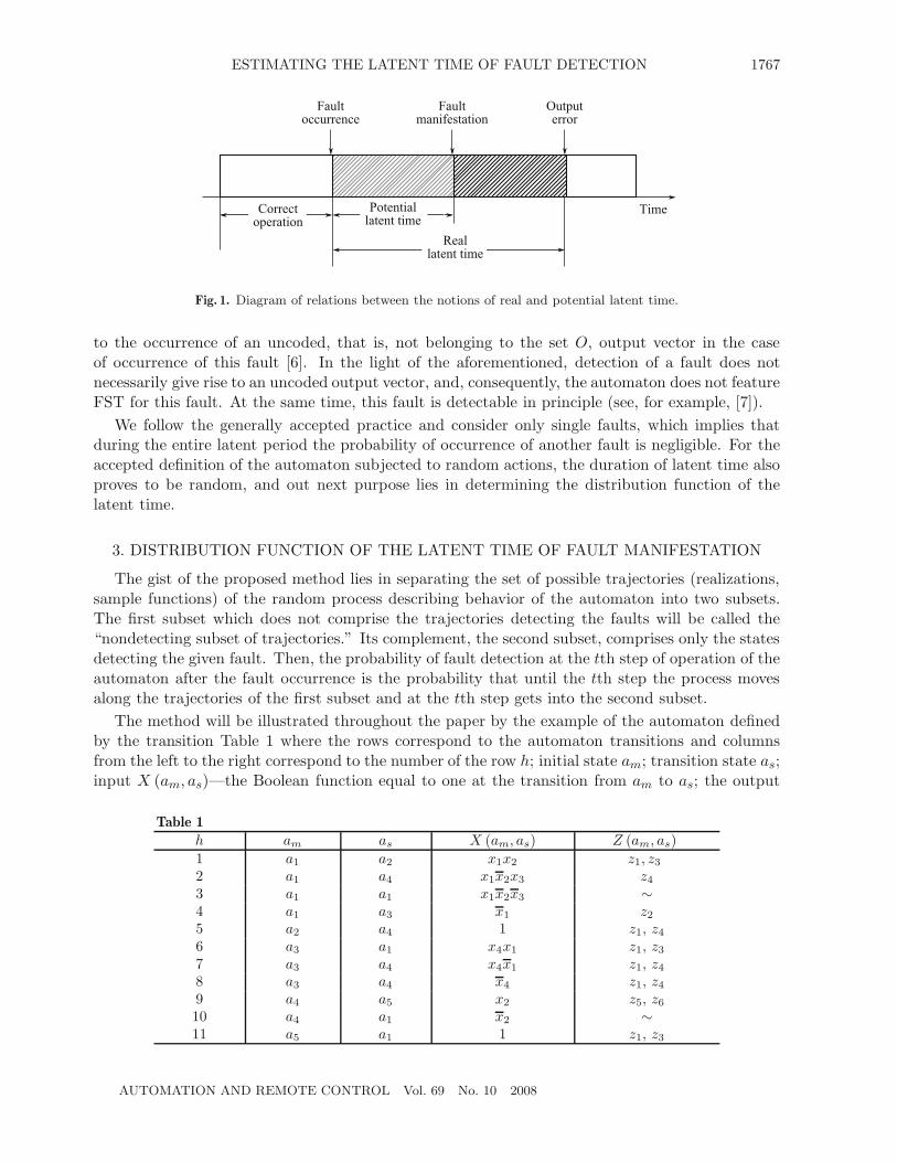
It is generally accepted to define the latent time of fault detection as the time interval betweenthe instants of its occurrence and manifestation [1]. By contrast, we consider the fault manifestationas any deviation of the automaton from the correct behavior that was caused by an impairment,regardless of occurrence of the output errors, and in this connection give the following definitions.

Definition 1. The potential latent time of fault manifestation is the time interval between theinstant of fault occurrence and the instant of any its manifestation.

Definition 2. The real latent time of fault manifestation at some observed point(s) is the timebetween instant of occurrence of this fault and the instant of its manifestation there.

As may be seen from Definition 1, for the automaton tested in real time the potential latenttime is the theoretically feasible minimal time of fault detection. As for the real latent time, itrefers to a particular observation point(s), usually to that (those) to which the checker is connected.Therefore, the difference between the real and potential times is nonnegative, and its magnitudeindicates to the basic possibility of improving the checkers. Additionally, the real latent timegenerally is different for various points of observation. This relation of times is illustrated by Fig. 1and demonstrated by an example to be presented below.

According to the definition of self-testifiability which is the necessary condition for full self-testifiability (FST), for each fault there exists some input vector leading after some latent time

AUTOMATION AND REMOTE CONTROL Vol. 69 No. 10 2008

ESTIMATING THE LATENT TIME OF FAULT DETECTION 1767

Fault

occurrence

Fault

manifestation

Output

error

Time

Real

latent time

Potential

latent time

Correct

operation

Fig. 1. Diagram of relations between the notions of real and potential latent time.

to the occurrence of an uncoded, that is, not belonging to the set O, output vector in the caseof occurrence of this fault [6]. In the light of the aforementioned, detection of a fault does notnecessarily give rise to an uncoded output vector, and, consequently, the automaton does not featureFST for this fault. At the same time, this fault is detectable in principle (see, for example, [7]).

We follow the generally accepted practice and consider only single faults, which implies thatduring the entire latent period the probability of occurrence of another fault is negligible. For theaccepted definition of the automaton subjected to random actions, the duration of latent time alsoproves to be random, and out next purpose lies in determining the distribution function of thelatent time.

3. DISTRIBUTION FUNCTION OF THE LATENT TIME OF FAULT MANIFESTATION

The gist of the proposed method lies in separating the set of possible trajectories (realizations,sample functions) of the random process describing behavior of the automaton into two subsets.The first subset which does not comprise the trajectories detecting the faults will be called the“nondetecting subset of trajectories.” Its complement, the second subset, comprises only the statesdetecting the given fault. Then, the probability of fault detection at the tth step of operation of theautomaton after the fault occurrence is the probability that until the tth step the process movesalong the trajectories of the first subset and at the tth step gets into the second subset.

The method will be illustrated throughout the paper by the example of the automaton definedby the transition Table 1 where the rows correspond to the automaton transitions and columnsfrom the left to the right correspond to the number of the row h; initial state am; transition state as;input X (am, as)—the Boolean function equal to one at the transition from am to as; the output

Table 1

h am as X (am, as) Z (am, as)1 a1 a2 x1x2 z1, z3

2 a1 a4 x1x2x3 z4

3 a1 a1 x1x2x3 ∼4 a1 a3 x1 z2

5 a2 a4 1 z1, z4

6 a3 a1 x4x1 z1, z3

7 a3 a4 x4x1 z1, z4

8 a3 a4 x4 z1, z4

9 a4 a5 x2 z5, z6

10 a4 a1 x2 ∼11 a5 a1 1 z1, z3


1768 GOOT, LEVIN

binary vector Z (am, as) at the transition from am to as. The output vector is set down as a list ofbinary signals zi equal to one. If none of them is equal to one, then the corresponding row carriesthe symbol “∼.”

In what follows, consideration is given to the faults of input, output, and state variables. Bythe faults of variables are meant faults like “suck-at-1” or “suck-at-0” (xl/1, xl/0). Additionally,the checker faults are considered as well.

3.1. Distribution of Latent Time under Faults of Input Variables

We use the following notation for the probabilities of values of the input variables xl:

Pr (xl = 1) = pl, Pr (xl = 0) = Pr (xl = 1) = ql = 1 − pl, l = 1, . . . , Nx.

Then, in the case of no faults behavior of the automaton obeys the Markov chain with thefollowing matrix of transition probabilities:

(pms) =

⎛⎜⎜⎜⎜⎜⎝

p1q2q3 p1p2 q1 p1q2p3 00 0 0 1 0

p1p4 0 0 q1p4 + q4 0q2 0 0 0 p2

1 0 0 0 0

⎞⎟⎟⎟⎟⎟⎠

. (1)

Let a fault like x1/1 occur for the input variable x1. We denote by A the manifestation ofoccurred fault and by A the opposite event. Now, we construct two matrices for the even A. Thefirst matrix is for the case of x1 = 1, and the second matrix, for x1 = 0. Then, the fault x1/1coincides with x1 if x1 = 1, and consequently, in this case it cannot manifest itself. The first matrixis obtained from (1) be substituting 1 and 0, respectively, for p1 and q1:

(pms | A,x1/1, x1 = 1

)=

⎛⎜⎜⎜⎜⎜⎝

q2q3 p2 0 q2p3 00 0 0 1 0p4 0 0 q4 0q2 0 0 0 p2

1 0 0 0 0

⎞⎟⎟⎟⎟⎟⎠

. (2)

The second matrix corresponds to x1= 0 and as follows from Table 1 has the form

(pms | A, x1/1, x1 = 0

)=

⎛⎜⎜⎜⎜⎜⎝

0 0 0 0 00 0 0 1 00 0 0 q4 0q2 0 0 0 p2

1 0 0 0 0

⎞⎟⎟⎟⎟⎟⎠

. (3)

The matrix of transition probabilities for the cases of A and x1/1 is as follows:(pms | A, x1/1

)= p1

(pmsA,x1/1, x1 = 1

)+ q1

(pms | A,x1/1, x1 = 0

)

=

⎛⎜⎜⎜⎜⎜⎝

p1q2q3 p1p2 0 p1q2p3 00 0 0 1 0

p1p4 0 0 q4 0q2 0 0 0 p2

1 0 0 0 0

⎞⎟⎟⎟⎟⎟⎠

. (4)



1

0 5 10 15 20 25

t

F ( t

)

Fig. 2. Graph of the latent time distribution function.

We stress that each of the matrices (2)–(4) describes only those transitions where faults cannotmanifest themselves, rather than every possible transition. Therefore, the matrices can be otherthan only stochastic, that is, the sum of elements in some rows needs not to be equal to one.

Let now

p(t − 1, A | x1/1

)=(p1

(t − 1, A | x1/1

), . . . , pNQ

(t − 1, A | x1/1

))

be the vector of probabilities of the automaton states at the (t − 1)st step after fault occurrence,but before its manifestation. We introduce the column vector

pT (A | x1/1) = (pms) (1, 0, 0, 1, 0)T (5)

with ones at the places of states detecting the fault, T being the sigh of transposition. Vector (5)defines the probabilities of states detecting faults on one step. Then, the probability Pf (t) ofdetecting x1/1 at the tth step is representable as

Pf (t) = p(t − 1, A | x1/1

)pT (A | x1/1) , (6)

and the vector p(t − 1, A | x1/1) is obtained at that using the recurrent formula

p(t − 1, A | x1/1

)= p

(t − 2, A | x1/1

) (pms | A,x1/1

), (7)

and p(0, A | x1/1) is the vector of probabilities of the automaton states at the instant of faultoccurrence.

Figure 2 depicts the results of calculating the additional distribution function of the latent time,that is, the probability that the latent time is greater than t,

F (t) = Pr (lat > t) =∞∑

k=t+1

Pf (k) = 1 −t∑

k=0

Pf (k) .

We consider the fault x4/1 (see transitions 7 and 8 in Table 1) in order to demonstrate thedifference between the potential and real latent times of detection. These transitions initiate thesame output vector. We emphasize that the fault x4/1 belongs namely to x4 (transition 7) and notto its negation (transition 8). For the accepted fault , if the (input) literals x1 = 0 and x4 = 0, thenboth corresponding terms are equal to one. Therefore, at the output of the automaton the faultmanifestation detected by term 7 will be masked by term 8. An example of difference between


1770 GOOT, LEVIN

1

0 10 20 30 40

t

F

1(

t

),

F

2(

t

)

50 60

F

1(

t

)

F

2(

t

)

Fig. 3. Graph of the distribution function of the real and potential latent times for the fault x4/1.

the distribution functions of the potential and real (relative to the output) latent times for thefault x4/1 is shown in Fig. 3.

The considered fault can be detected by the architecture using various observation points [7].In this case, the real (relative to the observation points used) and potential latent times coincide,which means that it is impossible to construct a better checker for the given fault. For other faults,this result in principle can be improved.

As follows from the above example, fault manifestation does not necessarily lead to its detec-tion at the output. Consequently, for this fault the given automaton features FST. However, thearchitecture of [7] enables one to detect it, although it does not manifest itself at the output.

3.2. Distribution of the Latent Time under Faults of the Output Variables

Let the fault z1/1 occur. It does not manifest itself if the output vector containing the variable z1

is not initiated (see states a2, a3, and a5 in Table 1). We use the above method to specify on theentire set of trajectories a subset such that it does not allow manifestation of this fault. As isevident from Table 1, the matrix corresponding to this subset is as follows:

(pms

(A))

=

⎛⎜⎜⎜⎜⎜⎝

0 0 0 0 00 0 0 1 0

p1p4 0 0 q1p4 + q4 00 0 0 0 01 0 0 0 0

⎞⎟⎟⎟⎟⎟⎠

.

The matrix corresponding to the faulty state is as follows:

(pms (A)) =

⎛⎜⎜⎜⎜⎜⎝

p1q2q3 p1p2 q1 p1q2p3 00 0 0 0 00 0 0 0 0q2 0 0 0 p2

0 0 0 0 0

⎞⎟⎟⎟⎟⎟⎠

,

and (pms(A)) + (pms(A)) = (pms).The distribution function of the latent time, that is, the fault manifestation probability at the

tth step, is as follows:

Pf (t) = p(0, A | y1/1

) (pms

(A))t−1

(pms (B)) (1, 1, 1, 1, 1)T , (8)

where p(0, A | y1/1) is the vector of automaton state at the instant of fault occurrence.



3.3. Distribution of the Fault Latent Time in the Memory of Automaton

If the state of the automaton memory is coded by a nonredundant code, then the fault cannotbe detected. In the case of redundant codes, the latent time of detection depends on the codecharacteristics. We assume by way of example that the unit position code is used. Then, for thestate ar a fault like yr/0 can be detected immediately at the instant of reaching this state, and thefault yr/1 manifests itself at the first step when the memory gets into a state other than ar.

We put down the matrix of transition probabilities in the general form

(pms) =

⎛⎜⎜⎜⎜⎜⎝

p1,1 . . . p1,r−1 p1,r p1,r+1 . . . p1,NQ

. . . . . . . . . . . . . . . . . . . . . . . . . . . . . . . . . . . . . . . . . . . . . . . .pr,1 . . . pr,r−1 pr,r pr,r+1 . . . pr,NQ

. . . . . . . . . . . . . . . . . . . . . . . . . . . . . . . . . . . . . . . . . . . . . . . .pNQ,1 . . . pNQ,r−1 pNQ,r pNQ,r+1 . . . pNQ,NQ

⎞⎟⎟⎟⎟⎟⎠

. (9)

The matrix specifying the set of trajectories that do not detect the fault yr/0 has zeros at therth row and the rth column:

(p(f)

ms

)=

⎛⎜⎜⎜⎜⎜⎝

p1,1 . . . p1,r−1 0 p1,r+1 . . . p1,NQ

. . . . . . . . . . . . . . . . . . . . . . . . . . . . . . . . . . . . . . . . . . .0 . . . 0 0 0 . . . 0

. . . . . . . . . . . . . . . . . . . . . . . . . . . . . . . . . . . . . . . . . . .pNQ,1 . . . pNQ,r−1 0 pNQ,r+1 . . . pNQ,NQ

⎞⎟⎟⎟⎟⎟⎠

.

In the example, matrix (9) has form (1). If the column vector

p(0) =(p1(0), . . . , pNQ

(0))

is the probability vector of the initial state (at the instant of fault occurrence), then the distributionof the latent time—the probability that the fault does not manifest itself before the kth step—isrepresentable as

Pr (t > k) = pr (0)(p(f)

ms

)k(1, . . . , 1, 0, 1, . . . , 1)T ,

with zero at the rth position.For the fault yr/1, we get

Pr (t = 1) = p (0)(p(f)

ms

)(1, . . . , 0, . . . , 1)T , Pr (t > k) = pr (0) pk

r,r,

where pr(0) is the rth element of the vector p(0) and pr,r is an element of matrix (9).

3.4. Distribution of the Latent Time of Checker Faults

The desired distribution is obtained using the method of construction of the matrices (pms(A))and (pms(A)). According to Table 1, these matrices as follows:

(pms

(A | R1/1

))=

⎛⎜⎜⎜⎜⎜⎝

0 0 q1 0 00 0 0 1 0

p1p4 0 q4 0 0p2 0 0 0 01 0 0 0 0

⎞⎟⎟⎟⎟⎟⎠

, (pms (A | R1/1))=

⎛⎜⎜⎜⎜⎜⎝

p1q2q3 p1p2 q1 p1q2p3 00 0 0 0 00 0 q1p4 0 00 0 0 0 q2

1 0 0 0 0

⎞⎟⎟⎟⎟⎟⎠

.

In order to determine the distribution function of the latent time, (8) must be applied with the useof p(0, A | R1/1).


1772 GOOT, LEVIN

4. ESTIMATION OF THE LATENT TIME OF FAULT MANIFESTATIONS

The above method for calculation of distributions describes exhaustively the latent time as arandom variable. It might seem that it requires a great bulk of computations. Yet if one uses in (6)the recurrent formula (7) and takes into consideration that the matrices of transition probabilitiesfor the generally accepted automata (matrix (1) in the case at hand) usually are very sparse andthe reasonably designed programs perform calculations only over the nonzero elements, the timeof calculations may prove to be quite acceptable.

At the same time, another reason must be taken into consideration. Calculation of the distribu-tion function of the latent time requires a rather great amount of initial data which are not alwaysavailable, especially at the initial stages of design. At that, it is possible to confine oneself to one oranother estimate of the latent time. Therefore, despite the aforementioned possibilities of reducingthe time required for precise calculations, the question of approximate estimates is of significantinterest.

Let us consider two approaches to getting such estimates:—determination of the upper and lower boundaries of the distribution function of the latent

time;—determination of the upper boundary of the mean value of the latent time.

4.1. The Lower and Upper Boundaries of the Latent Time Distribution

Let the latent time distribution for the fault f obey (6)—example for f = x1/1. Then, (6)and (7) are representable as

Pf (t) = p(t − 2, A | x1/1

) (pms | A,x1/1

)pT (A | x1/1) . (10)

Let us determine

pT (A | x1/1) =(α1, . . . , αNQ

)(11)

and(pms | A,x1/1

)pT (A | x1/1) =

(β1, . . . , βNQ

), (12)

where αi is the sum of the probabilities of transition from the state ai to the state manifesting thefault under consideration.

We rearrange (12) in(pms | A,x1/1

)pT (A | x1/1) = (γ1α1, . . . , γNQ

αNQ), γi = βi/αi ≤ 1, αi �= 0, (13)

substitute (13) in (10)

Pf (t) = p(t − 2, A | x1/1

)(γ1α1, . . . , γNQ

αNQ)

∣∣∣∣∣∣≤ p

(t − 2, A | x1/1

)γmax

(α1, . . . , αNQ

)

≥ p(t − 2, A | x1/1

)γmin

(α1, . . . , αNQ

),

(14)

γmax = maxi

γi, γmin = mini

(γi | γi �= 0) ,

and use (10) and (11) to represent (14) as

Pf (t) ≤ γmaxPf (t − 1) = Pmaxf (t) ,

Pf (t) ≥ γminPf (t − 1) = Pminf (t) .

(15)



Relation (15) enables one to estimate the residual part of the function Pf (t) at any step afterprecise calculations or to give the following exponential estimates:

Pf (t) ≤ γtmaxp (0, A | x1/1) ,

Pf (t) ≥ γtminp (0, A | x1/1) .

(16)

We note that if all γi are equal, γi = γ, then inequalities (27) turn into equalities, that is, providethe exact expression for the function Pf (t) which is exponential in this case:

Pf (t) = γtp (0, B | x1/1) .

If γmax = 1, then the first formula in (15) becomes trivial and other methods of estimation mustbe sought.

4.2. Upper Boundary of the Mean Value of Latent Time

To establish the desired estimates, we construct in this case a “worst” automaton and alsoassume that Pr(xl = 1) = 0.5 for any xl.

The set of terms will be said to be the “triangular” set of length K ≤ Nx if

GK+1 =K∏

l=1

xl; Gk =k−1∏l=1

xlxk, k = 1, . . . ,K. (17)

Then, the two following theorems are valid.

Theorem 1. For the automaton with identical probabilities of fault occurrence and the set oftransition functions defined by the “triangular” set of terms, the mean probability of manifestationof a single fault is minimal over every possible automaton with the same number of states andequal to

pf =1K

(1 − 1

2K

).

Theorem 2. Among all automata with NQ states and Nx input variables, the automaton of Fig. 4has the following maximal latent time per one fault:

T =2NQ

Nx

(2Nx − 1

)−(

NQ

2+ 1

). (18)

We note that the determined estimate T is unimprovable because the structure of the automatonwhere it is reached is given.

Theorems 1 and 2 are proved in the Appendix.

5. PROBABILITY OF RETENTION OF FAULT UNIQUENESS

It may turn out in practice that only the real latent time is of interest because over this periodthe automaton operates without faults (at outputs) and at appearance of an output fault it mustbe stopped. Therefore, the potential latent time will be only of theoretical interest as a possibleboundary of improvement of checkers.

Until now we followed the generally accepted way and assumed that the fault remains singleover the entire time between its occurrence and the instant of its manifestation. However, another


1774 GOOT, LEVIN

fault may occur between the instants of fault occurrence and manifestation. Moreover, this newfault can mask its predecessor so that the automaton will operate erroneously, but this fact willeither remain undetected at all or detected much later even relative to the real latent time of thesingle fault. In this situation the above methodology of estimation of the potential and real latenttimes proves to be unacceptable. However, to reduce the probability of occurrence of these eventsin any case it is required to reduce the time of fault detection and, consequently, the potentiallatent time becomes an essential characteristic.

The following two problems may be posed in the light of this fact: (a) examine the problem ofdetection of multiple faults, including the case of mutual masking, and (b) determine the probabilitythat a fault remains single until its manifestation and, consequently, the conditions for applicabilityof the above results remain valid. Now we turn to the second problem and leave the first problemfor separate study.

Let us numerate all possible faults and let their number be M . Also, let Pl(n) be the distributionfunction of the potential latent time for the lth fault and pm be the probability of occurrence ofthe mth fault l, m = 1, . . . ,M . Assuming that the instants of occurrence of different faults areindependent, we can set down the probability that the lth fault remains single over the entire latenttime as follows:

Ql =∞∑

n=0

Pl (n) × Pr (D) =∞∑

n=0

Pl (n)M∏

m=1m�=l

(1 − pm)n ,

where D is the case where no other fault appears over the entire latent time of occurrence of thelth fault.

For the standard case of pm 1, we obtain to within o(pm) that

Ql =∞∑

n=0

Pl (n)M∏

m=1m�=l

(1 − npm) =∞∑

n=0

Pl (n)

⎛⎜⎜⎝1 −

M∑m=1m�=l

npm

⎞⎟⎟⎠ = 1 − E (nl)

M∑m=1m�=l

pm,

where E(nl) is the mean latent time for the lth fault.We note that Ql is independent of the distribution of the latent time and depends only on its

mean value.The resulting probability characterizes the lth fault. In essence, it is the conditional probability

for the case of fault occurrence. For the unconditional probability we obtain the following:

Q =M∑l=1

plQl =M∑l=1

pl

⎛⎜⎜⎝1 − E (nl)

M∑m=1m�=l

pm

⎞⎟⎟⎠ . (19)

Now we turn to the probability of masking. Let the lth fault can be masked by the faultnumbered l1. For example, these may be the bit-stuck faults of some literal and its negation.Then, the probability that masking occurs before the instant of manifestation is as follows:

Rl =∞∑

n=0

Pl (n) [1 − (pl)]n

M∏m=1

m�=l,l1

(1 − pm)n .



For small pm, we obtain with the same precision that

Rl =∞∑

n=0

Pl (n)npl1

⎛⎜⎜⎝1 −

M∑m=1

m�=l,l1

npm

⎞⎟⎟⎠ = E (nl1) pl1 − E

(n2

l

) M∑m=1

m�=l,l1

pmpl1. (20)

The unconditional probability is obtained by multiplying (20) by pl summation over all l’s.

6. EXPERIMENTAL RESULTS

Five automata describing each operation of some microprocessor were used as experimentalbenchmarks whose parameters and the calculated latent times are compiled in Table 2, where Nx isthe number of inputs, Ny is the number of outputs, NQ is the number of states, h is the number ofthe transition, and t and T are the precise and maximal values of the mean latent time, respectively,as calculated from the ordinary formulas of expectation using (8) for t and (19) for T , time beingmeasured in cycles. Analysis of the results demonstrated utility of both methods for estimation ofthe latent time.

Table 2

Name Nx Ny NQ h t Tbig 18 28 17 185 747 2420bs 19 13 17 185 247 903acdl 16 27 22 214 456 1742cow 49 24 24 261 366 1486v1 6 14 18 17 169 237 608v1 10 15 18 18 264 300 907v11 20 14 29 18 367 360 1630

7. CONCLUSIONS

The above results may be summed up as follows.(1) The paper analyzed the latent time of manifestation of the occurring faults. This analysis

is valid for the case where the automaton is tested in the course of its real operation.(2) Introduced was the concept of the potential and real latent times. Their difference is in-

dicative of the potentiality of checker improvement, which is important for reduction of the faultdetection time and the probability of mutual masking in the case of multiple faults.

(3) A precise expression for calculation of the distribution of the potential and real latent times,as well as their upper boundaries, was established.

(4) An expression for the upper (worst) estimate of the mean latent time was obtained from theanalysis of the proposed construction of the “worst” automaton. The precise value of the meanlatent time is about 30% of the established upper boundary, which may be regarded as satisfactorytaking into consideration the fact that T is intended for estimation at that stage of design wherethe volume of data is limited.


1776 GOOT, LEVIN

APPENDIX

Proof of Theorem 1. Let us expand the “triangular” set of terms (17) as follows:

GK+1 = x1 x2 · · · xl · · · xK−1 xK ,GK = x1 x2 · · · xl · · · xK−1 xK ,GK−1 = x1 x2 · · · xl · · · xK−1,. . . . . . . . . . . . . . . . . . . . . . . .Gl = x1 x2 · · · xl,. . . . . . . . . . . . . . . . . . . .G2 = x1 x2,G1 = x1.

(A.1)

We first determine the initial probability of fault manifestation for a variable in (A.1). Forexample, let it be the variable x1 with a fault like x1/1, which means that all literals x1 in (A.1)are equal to one. If now the variable itself x1 = 0, then its value and those of its correspondingliterals in (18) are distinct. Therefore, the fault can manifest itself with the probability 0.5. For thesame reason, the probabilities of the fault x1/0 and the same faults for the literals correspondingto the negation of x1 are equal to 0.5 as well.

Now we consider the fault xl/1. As follows from (12), it can manifest itself only if∏

xk = 1,where the product is taken over all k < l. In this case we obtain the conditional and unconditionalmanifestation probabilities

pf

(xl

∣∣∣∣∣l−1∏k=1

xk = 1

)=

12,

pf (xl) = Pr

(l−1∏k=1

xk = 1

)pf

(xl

∣∣∣∣∣l−1∏k=1

xk = 1

)=(

12

)l

.

The probability of fault manifestation averaged over set (A.1) is as follows:

pf =1K

K∑l=1

pf (xl) =1K

(1 − 1

2K

).

It is assumed at that that the occurrence probabilities of all faults are the same.Proof of Theorem 2. Let the variable xl fail. As is evident from Fig. 4, the automaton structure

admits its manifestation only on the transition from a1 to a2, and pf (xl) = 1/2l is the probabilityof this manifestation.

a

1

a

3

a

NQ

1 1

1

G

Nx

+1

G

Nx

G

2

G

1

a

2

Fig. 4. Graph of the “worst” automaton, that is, the automaton with the maximum mean latent time.



If there was no fault manifestation, conditions for its manifestation will appear only after NQ−1step when the automaton again returns to the state a1. Under the accepted conditions, the number rof cycles before manifestation is a random variable obeying the geometrical distribution

Pl (r) = (1 − pf (xl))r−1 pf (xl) .

The mean number of states to be passed by the automaton from the instant of fault occurrence tothat of its manifestation, provided that the fault occurs at the instant where the automaton is inthe state a1, is as follows:

Tl (a1) =∞∑

r=1

[(r − 1) NQ + 1]Pl (r) = NQ

∞∑r=1

rqr−1f (xl) pf (xl)

= NQ

(1

pf (xl)− 1

)− 1 = NQ

(2l − 1

)− 1.

If we assume now that a fault arises with equal probability at the instant when the automaton isin any state, then the unconditional mean latent time of manifestation will be as follows:

T l = T l (a1) +NQ

2.

Finally, by averaging over all feasible single faults and assuming that all faults are equiprobable,we obtain the following mean latent time

T =1

Nx

NQ∑l=1

T l =NQ

Nx

L∑l=1

2l −(

NQ

2− 1

)=

2NQ

Nx

(2Nx − 1

)−(

NQ

2− 1

).

REFERENCES

1. Lala, P., Self-Checking and Fault Tolerant Digital Design, San Francisco: Morgan Kaufman, 2000.

2. Shedletsky, J. and McCluskey, E., The Error Latency of Fault in a Sequential Digital Circuit, IEEETrans. Comput., 1976, vol. 25, no. 6, pp. 655–659.

3. Goot, R., Levin, I., and Ostanin, S., Fault Latencies of Concurrent Checking FSMs, in Proc. DSD 2002Euromicro Sympos. Digital Syst. Design Architectures, Methods and Tools, Dortmund, pp. 174–179.

4. Feller, W., An Introduction to Probability Theory and Its Applications , New York: Wiley, 1971.

5. Kemeny, J. and Snell, J., Finite Markov Chains , Princeton: Van Nostrand, 1967.

6. Nicolaidis, M. and Zorian, Y., On-line Testing for VLSI—A Compendium of Approaches, J. Electron.Testing: Theory Appl., 1998, no. 12, pp. 7–20.

7. Levin, I. and Sinelnikov, V., Self-checking of FPGA based Control Units, in Proc. Great Lakes Sympos.VLSI , Ann Arbor: IEEE Press, 1999, pp. 292–295.

This paper was recommended for publication by P.P. Parkhomenko, a member of the EditorialBoard


estimating the latent time of fault detection in finite automaton tested in real time

Documents