Estimating the Health Effects of

Ambient Air Pollution and Temperature

Bart Ostro, Ph.D., Chief

Air Pollution Epidemiology Section

Office of Environmental Health Hazard Assessment

California EPA

Hundreds of Epidemiological Studies of

Air Pollution and Dozens on Temperature

• Many different study designs

• Pros/cons for each

• Fostered by availability of health data and

monitoring of temperature and ubiquitous

pollutants

• Control for confounders

• Supported by human clinical and

toxicological studies

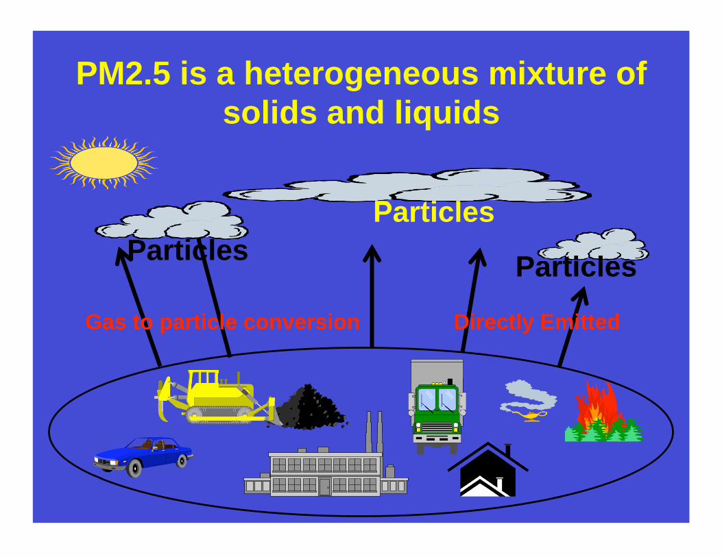
PM2.5 is a heterogeneous mixture of

solids and liquids

Particles

Particles

Gas to particle conversion Directly Emitted

Particles

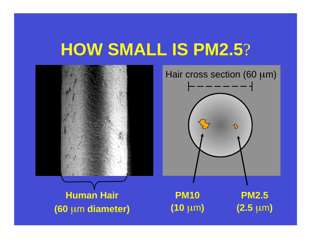
HOW SMALL IS PM2.5?

Human Hair

(60 μm diameter)

PM10

(10 μm)

PM2.5

(2.5 μm)

Hair cross section (60 μm)

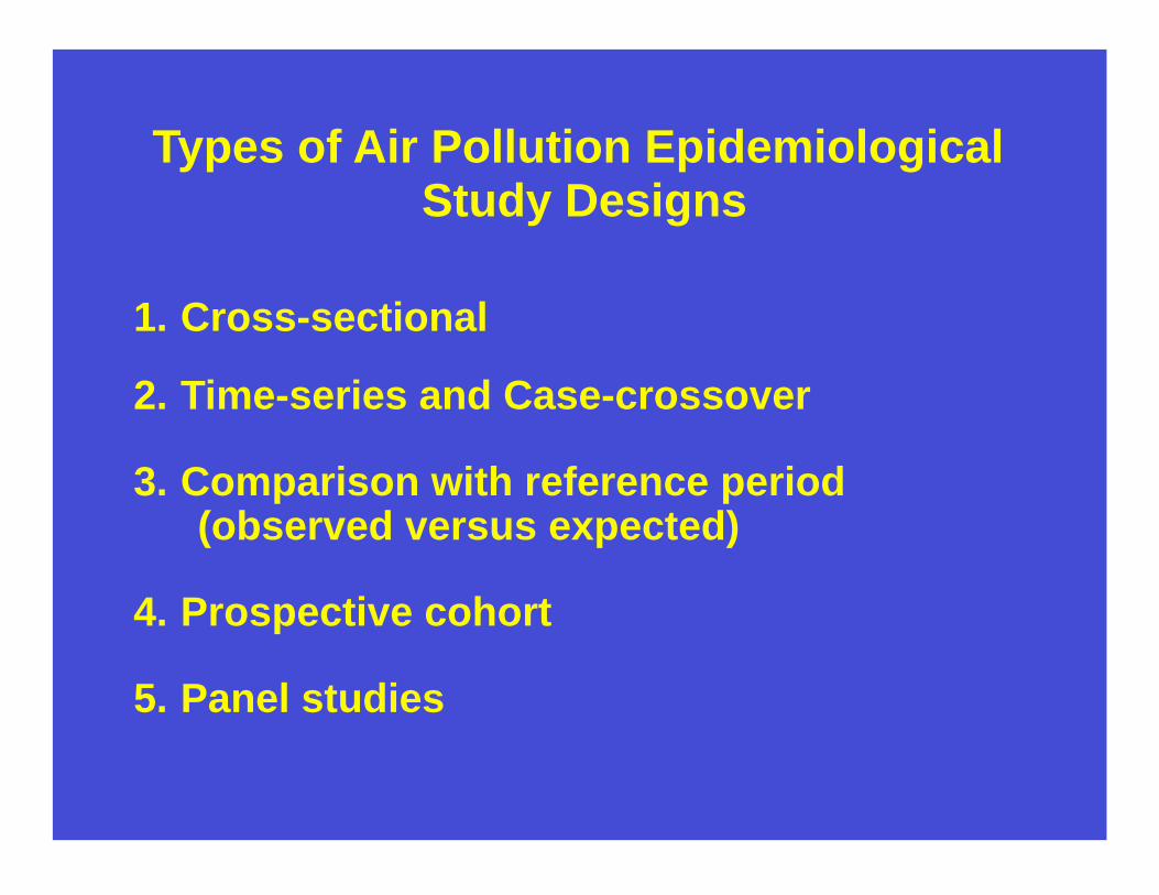
Types of Air Pollution Epidemiological Study Designs

1. Cross-sectional

2. Time-series and Case-crossover

3. Comparison with reference period (observed versus expected)

4. Prospective cohort

5. Panel studies

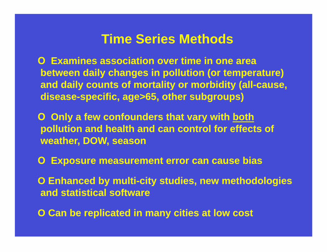
Time Series Methods

Examines association over time in one area

between daily changes in pollution (or temperature)

and daily counts of mortality or morbidity (all-cause,

disease-specific, age>65, other subgroups)

Only a few confounders that vary with both

pollution and health and can control for effects of

weather, DOW, season

Exposure measurement error can cause bias

O Enhanced by multi-city studies, new methodologies

and statistical software

O Can be replicated in many cities at low cost

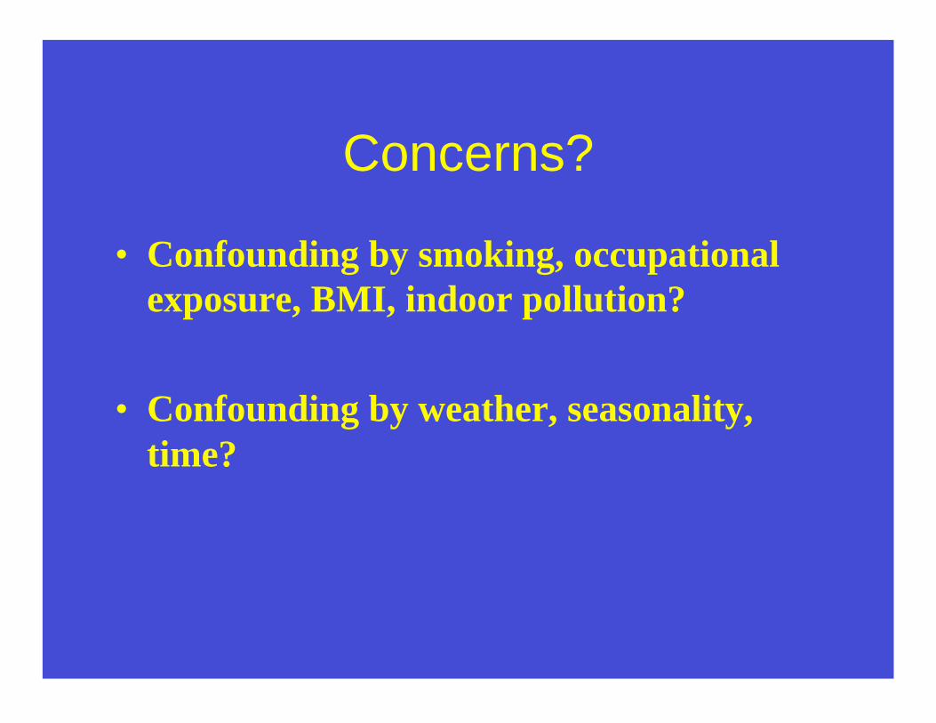
Concerns?

• Confounding by smoking, occupational

exposure, BMI, indoor pollution?

• Confounding by weather, seasonality,

time?

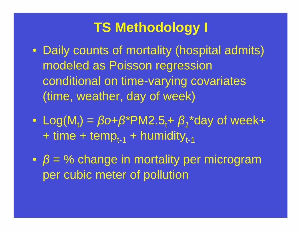
TS Methodology I

• Daily counts of mortality (hospital admits)

modeled as Poisson regression

conditional on time-varying covariates

(time, weather, day of week)

• Log(Mt) = o+ *PM2.5t+ 1*day of week+

+ time + tempt-1 + humidityt-1

• = % change in mortality per microgram

per cubic meter of pollution

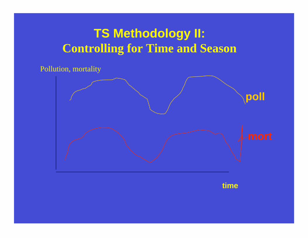
TS Methodology II:

Controlling for Time and Season

Pollution, mortality

time

poll

mort

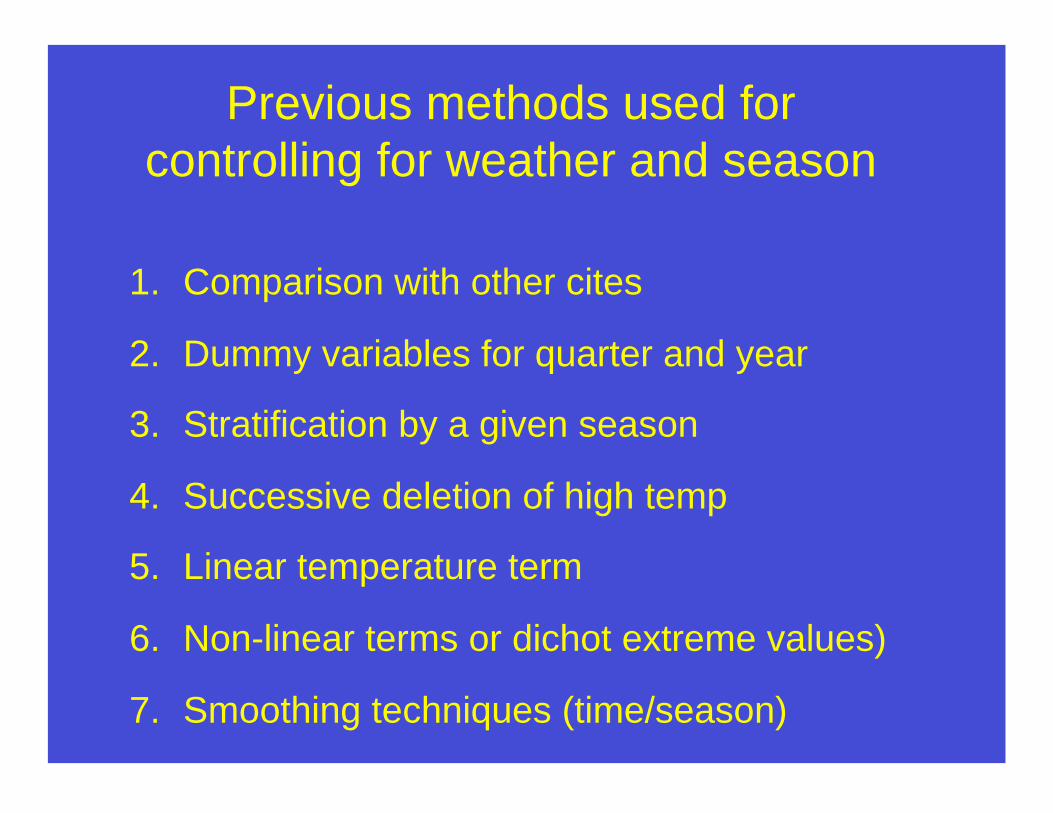
Previous methods used for

controlling for weather and season

1. Comparison with other cites

2. Dummy variables for quarter and year

3. Stratification by a given season

4. Successive deletion of high temp

5. Linear temperature term

6. Non-linear terms or dichot extreme values)

7. Smoothing techniques (time/season)

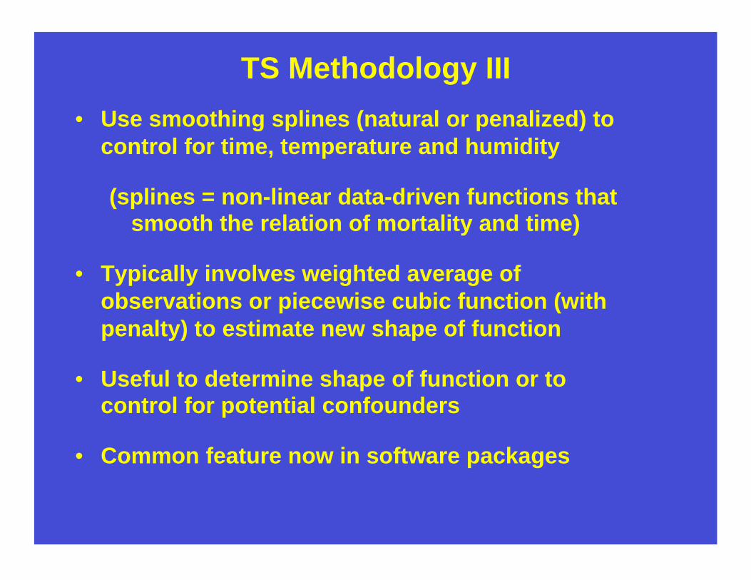
TS Methodology III

• Use smoothing splines (natural or penalized) to

control for time, temperature and humidity

(splines = non-linear data-driven functions that smooth the relation of mortality and time)

• Typically involves weighted average of

observations or piecewise cubic function (with

penalty) to estimate new shape of function

• Useful to determine shape of function or to control for potential confounders

• Common feature now in software packages

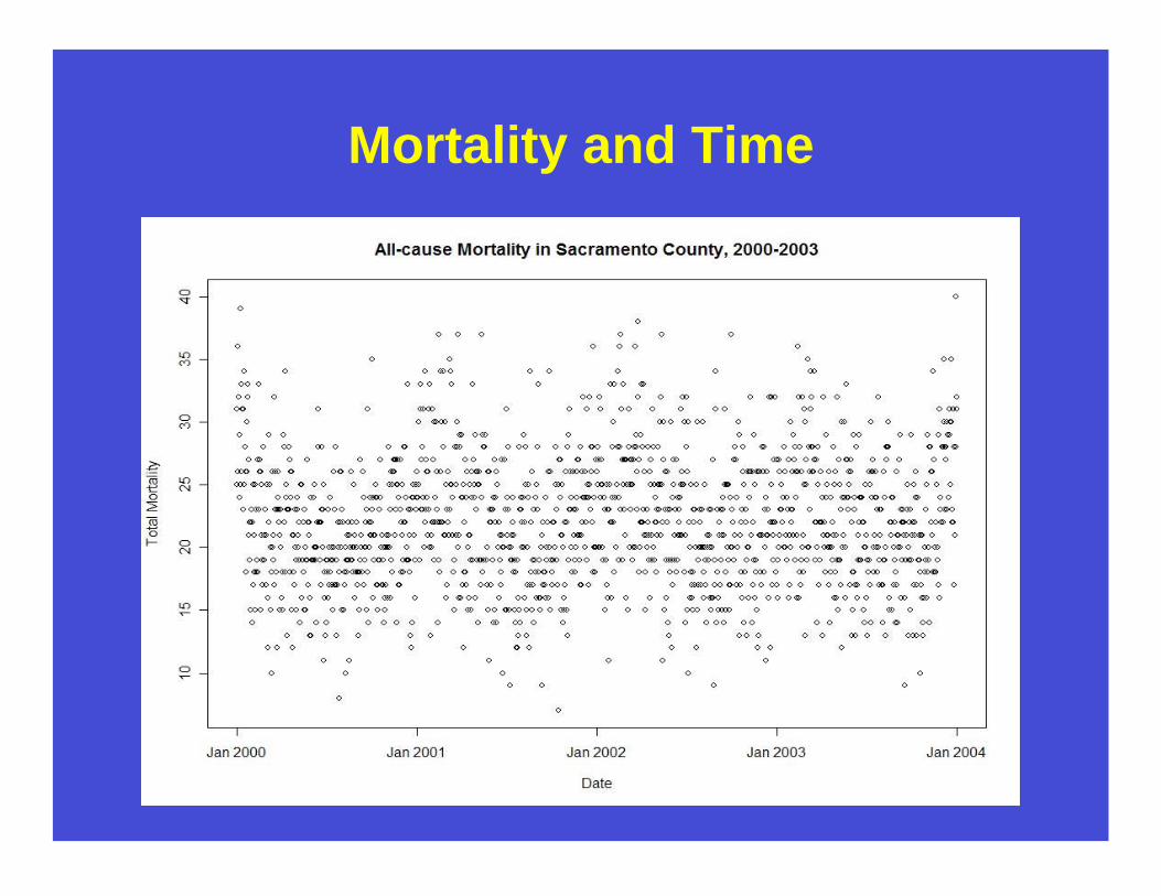
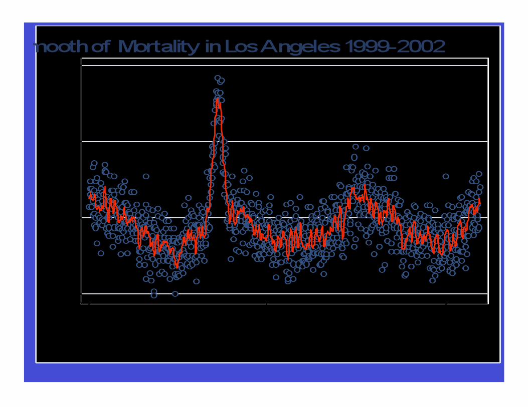
Mortality and Time

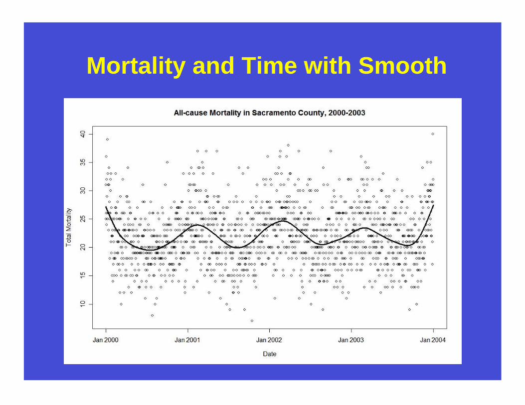
Mortality and Time with Smooth

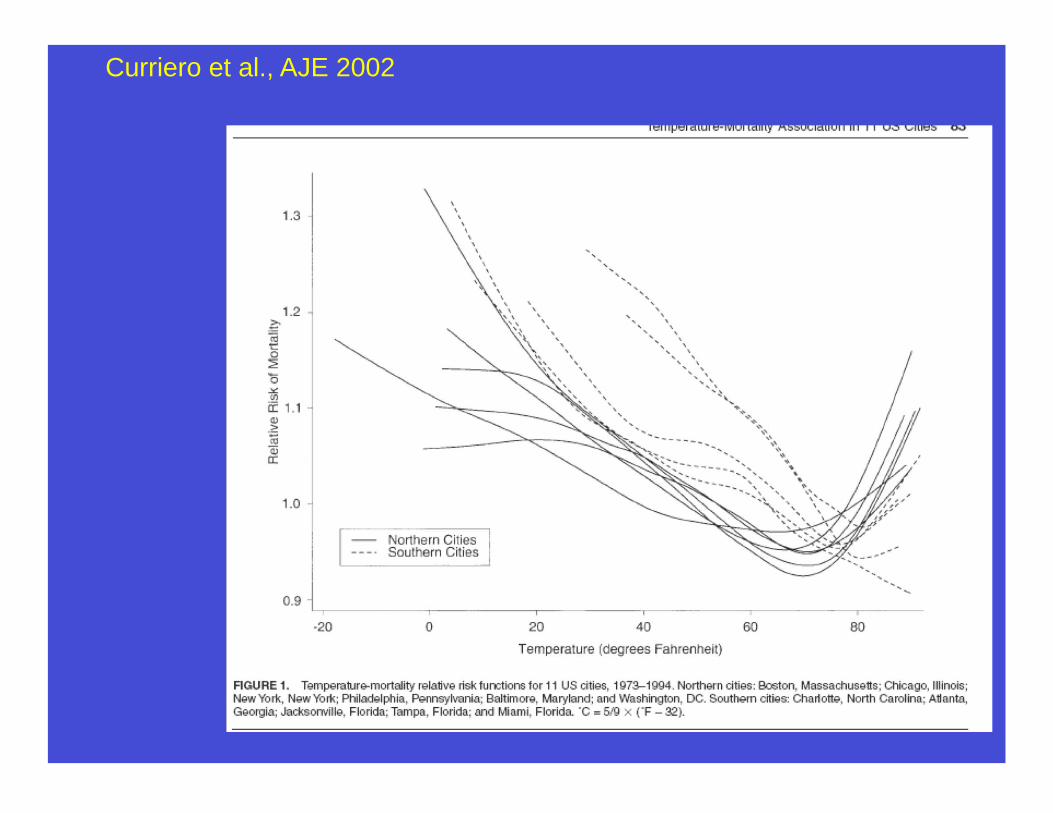
Curriero et al., AJE 2002

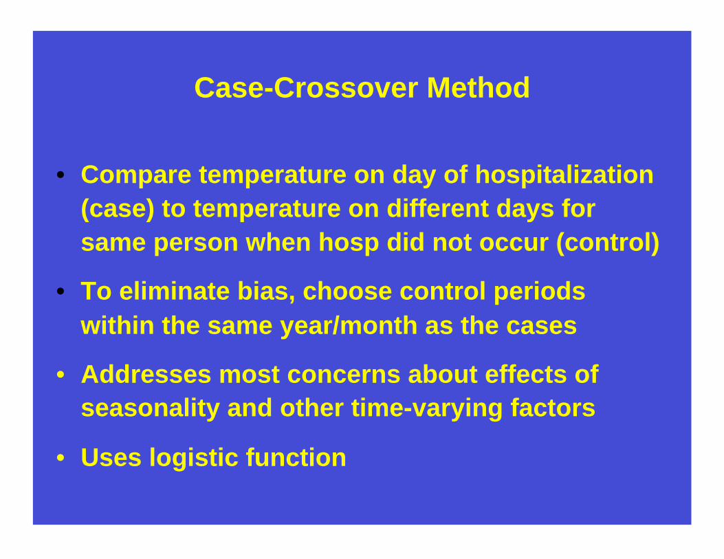
Case-Crossover Method

• Compare temperature on day of hospitalization

(case) to temperature on different days for

same person when hosp did not occur (control)

• To eliminate bias, choose control periods

within the same year/month as the cases

• Addresses most concerns about effects of

seasonality and other time-varying factors

• Uses logistic function

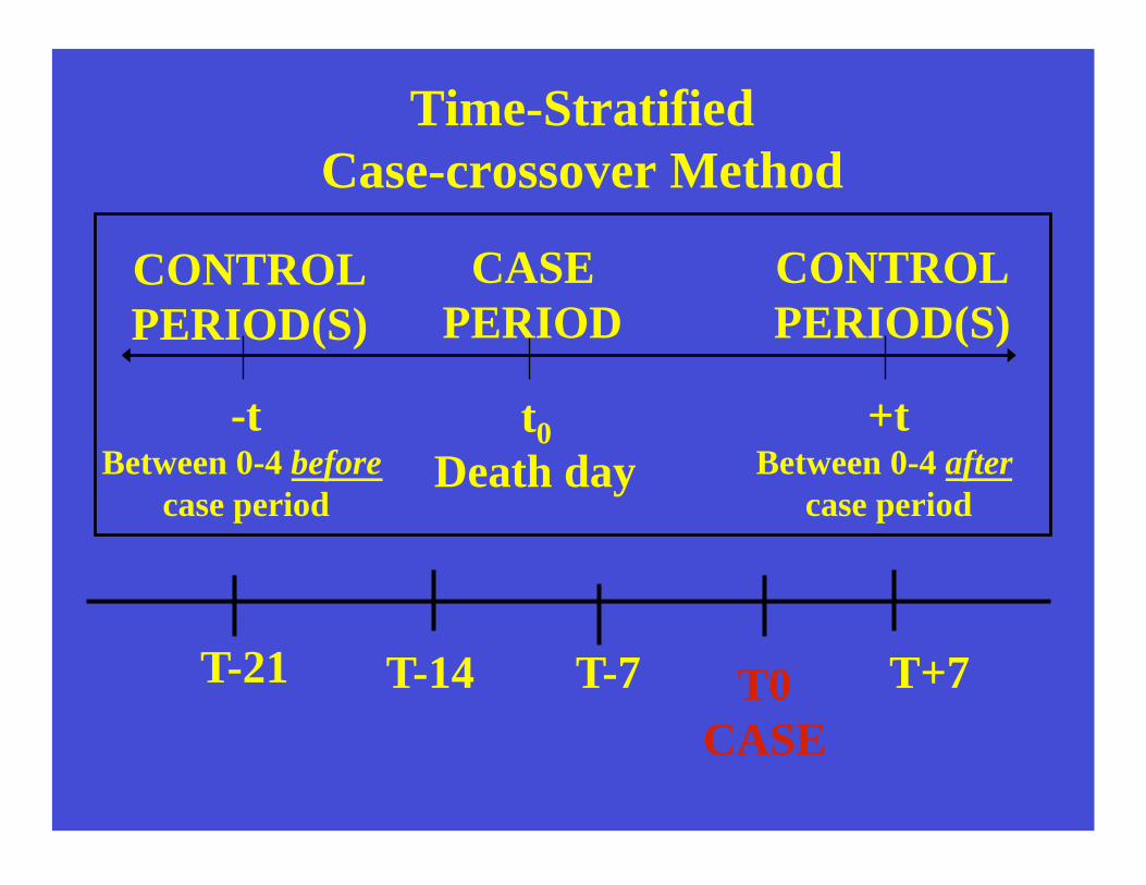
Time-Stratified

Case-crossover Method

CONTROL

PERIOD(S)

CASE

PERIOD

CONTROL

PERIOD(S)

-t Between 0-4 before

case period

t0

Death day

+t Between 0-4 after

case period

T-14 T-7 T0

CASE

T+7 T-21

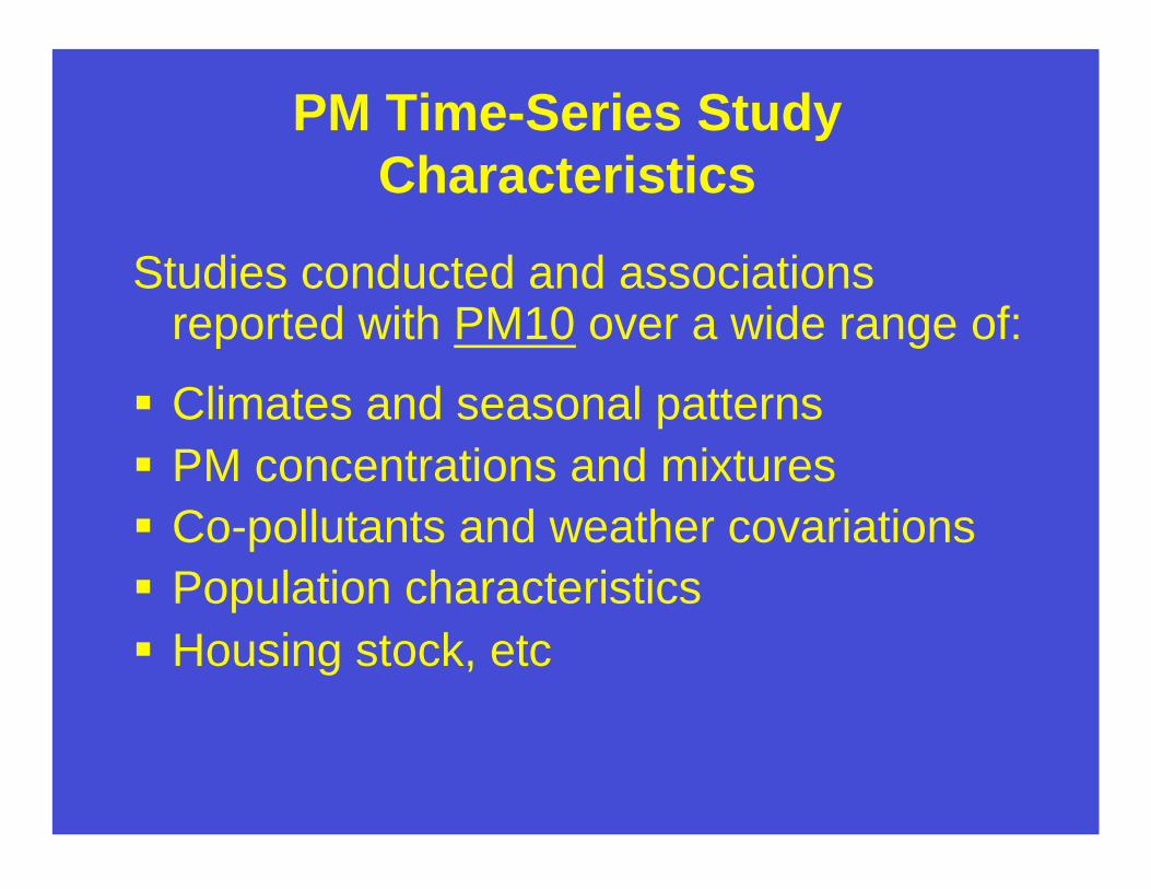
PM Time-Series Study

Characteristics

Studies conducted and associations reported with PM10 over a wide range of:

Climates and seasonal patterns

PM concentrations and mixtures

Co-pollutants and weather covariations

Population characteristics

Housing stock, etc

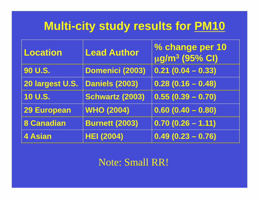
Location Lead Author % change per 10

μg/m3 (95% CI)

90 U.S. Domenici (2003) 0.21 (0.04 – 0.33)

20 largest U.S. Daniels (2003) 0.28 (0.16 – 0.48)

10 U.S. Schwartz (2003) 0.55 (0.39 – 0.70)

29 European WHO (2004) 0.60 (0.40 – 0.80)

8 Canadian Burnett (2003) 0.70 (0.26 – 1.11)

4 Asian HEI (2004) 0.49 (0.23 – 0.76)

Multi-city study results for PM10

Note: Small RR!

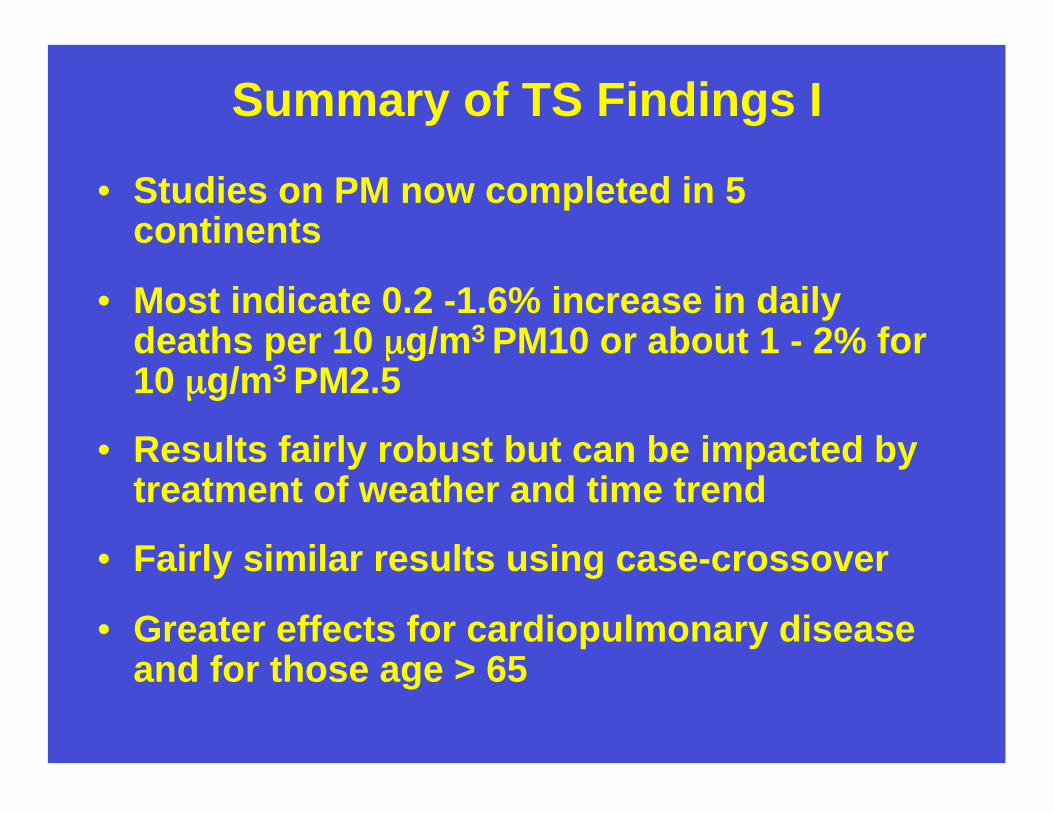
Summary of TS Findings I

• Studies on PM now completed in 5 continents

• Most indicate 0.2 -1.6% increase in daily deaths per 10 μg/m3 PM10 or about 1 - 2% for 10 μg/m3 PM2.5

• Results fairly robust but can be impacted by treatment of weather and time trend

• Fairly similar results using case-crossover

• Greater effects for cardiopulmonary disease and for those age > 65

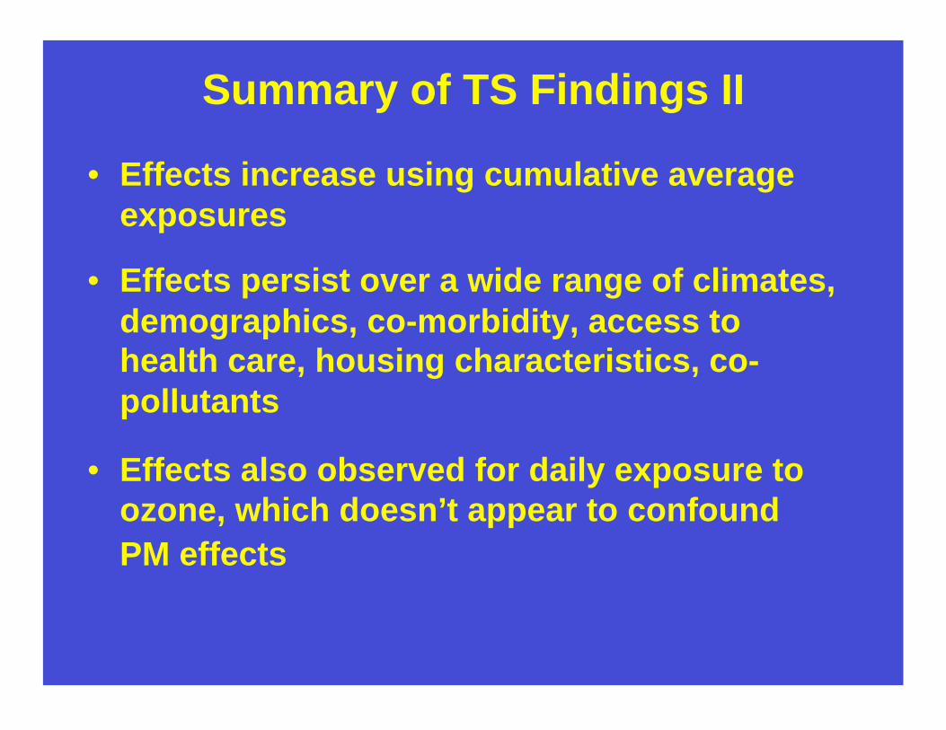
Summary of TS Findings II

• Effects increase using cumulative average

exposures

• Effects persist over a wide range of climates,

demographics, co-morbidity, access to

health care, housing characteristics, co-

pollutants

• Effects also observed for daily exposure to

ozone, which doesn’t appear to confound

PM effects

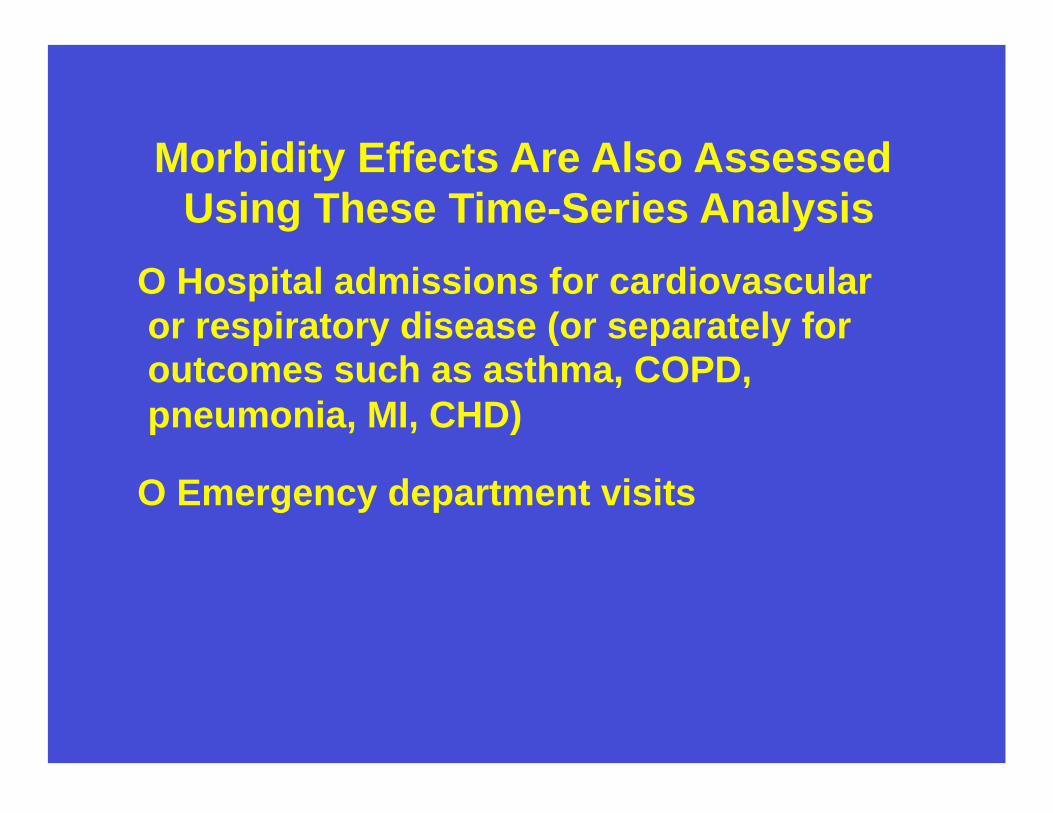
Morbidity Effects Are Also Assessed

Using These Time-Series Analysis

O Hospital admissions for cardiovascular

or respiratory disease (or separately for

outcomes such as asthma, COPD,

pneumonia, MI, CHD)

O Emergency department visits

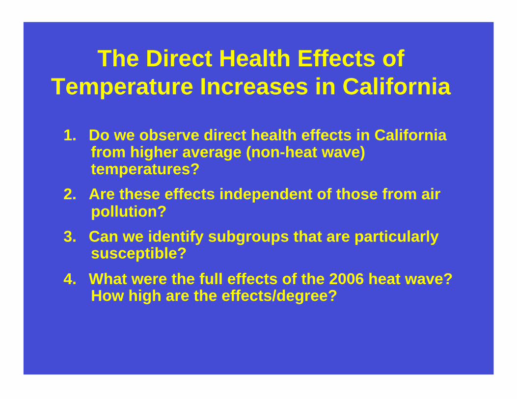
The Direct Health Effects of

Temperature Increases in California

1. Do we observe direct health effects in California from higher average (non-heat wave) temperatures?

2. Are these effects independent of those from air pollution?

3. Can we identify subgroups that are particularly susceptible?

4. What were the full effects of the 2006 heat wave? How high are the effects/degree?

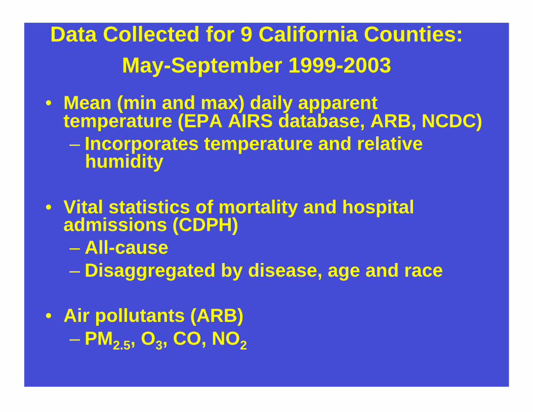
Data Collected for 9 California Counties:

May-September 1999-2003

• Mean (min and max) daily apparent temperature (EPA AIRS database, ARB, NCDC)

– Incorporates temperature and relative humidity

• Vital statistics of mortality and hospital admissions (CDPH)

– All-cause

– Disaggregated by disease, age and race

• Air pollutants (ARB)

– PM2.5, O3, CO, NO2

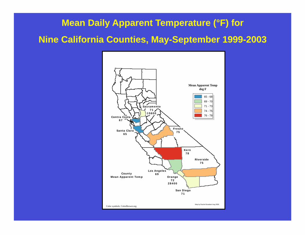
Mean Daily Apparent Temperature (°F) for

Nine California Counties, May-September 1999-2003

Kern 78

Fresno 75

Riverside 75

San Diego 71

Los Angeles 69

Santa Clara 65

Sacramento 71

15600 Contra Costa

67

Orange 72

28400

Map by Rachel Broadwin Aug 2006

County Mean Apparent Temp

Mean Apparent Temp deg F

65 - 68 69 - 70 71 - 73 74 - 75 76 - 78

Color symbols: ColorBrewer.org

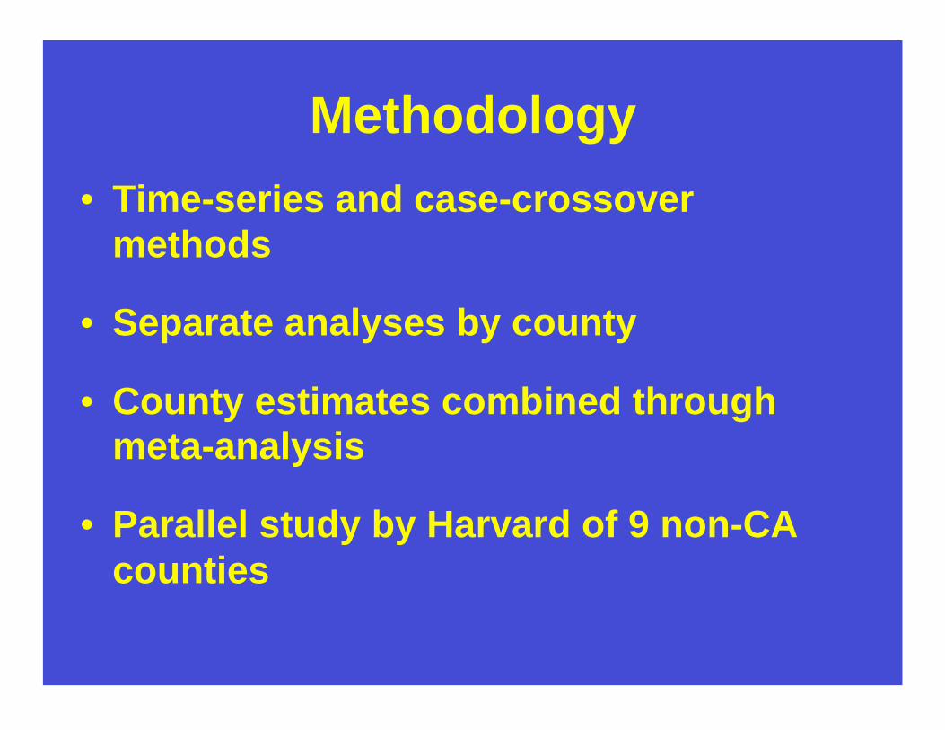
Methodology

• Time-series and case-crossover

methods

• Separate analyses by county

• County estimates combined through

meta-analysis

• Parallel study by Harvard of 9 non-CA

counties

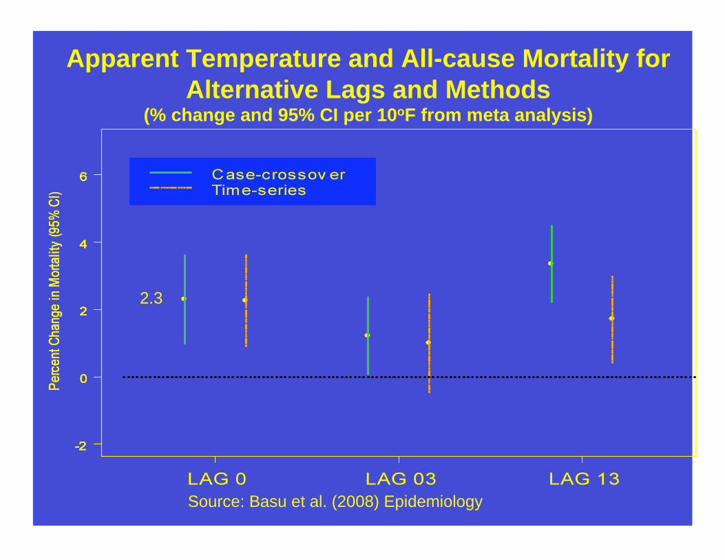
Apparent Temperature and All-cause Mortality for

Alternative Lags and Methods (% change and 95% CI per 10oF from meta analysis)

2.3

Source: Basu et al. (2008) Epidemiology

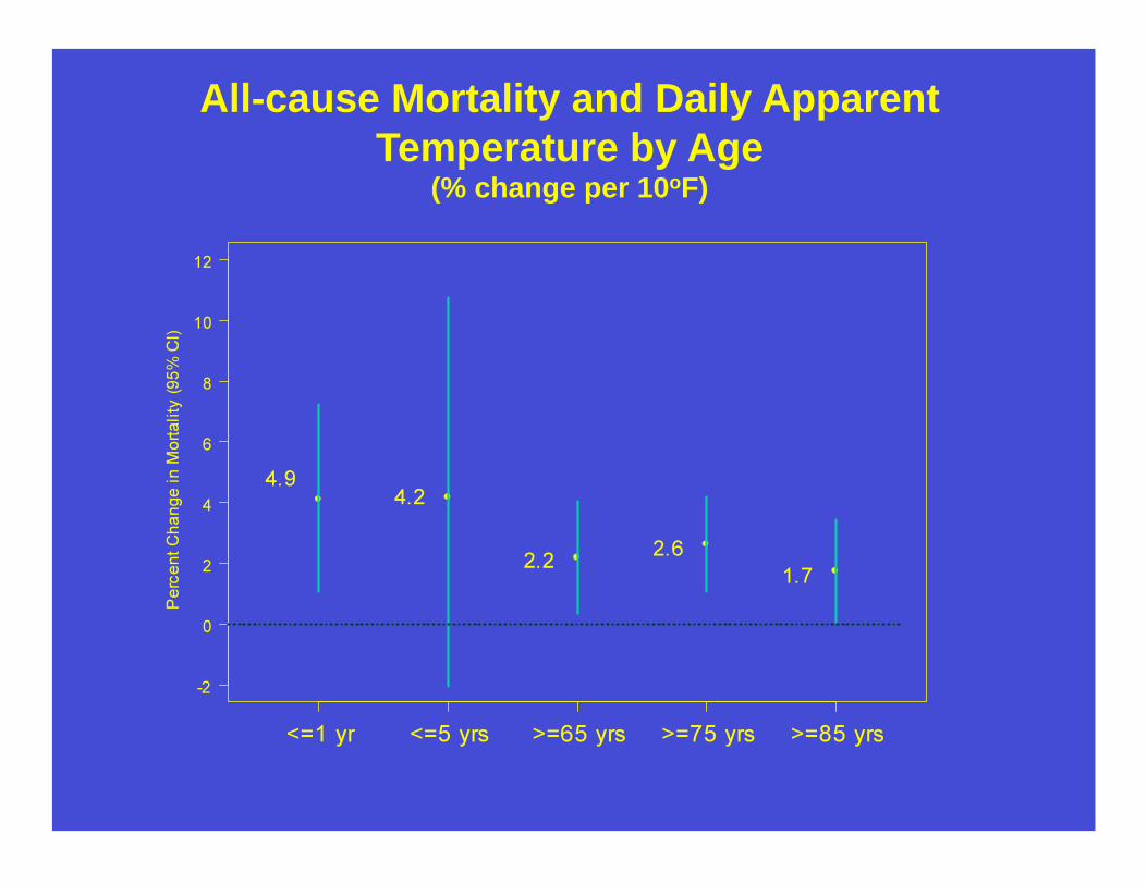
All-cause Mortality and Daily Apparent

Temperature by Age (% change per 10oF)

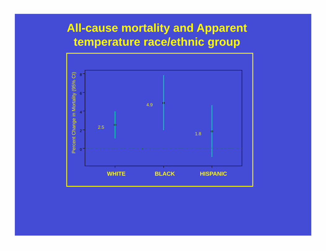
All-cause mortality and Apparent

temperature race/ethnic group

Perc

ent

Change in M

ort

alit

y (

95%

CI)

0

2

4

6

8

WHITE BLACK HISPANIC

2.5

4.9

1.8

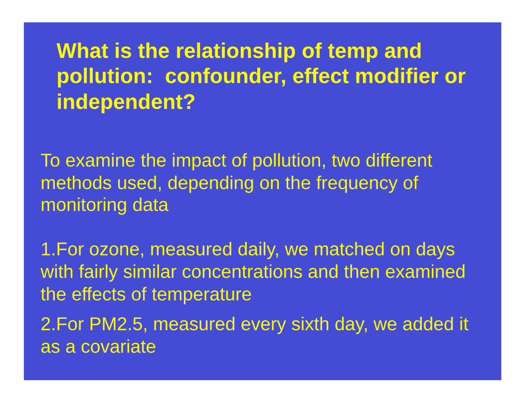
To examine the impact of pollution, two different

methods used, depending on the frequency of

monitoring data

1.For ozone, measured daily, we matched on days

with fairly similar concentrations and then examined

the effects of temperature

2.For PM2.5, measured every sixth day, we added it

as a covariate

What is the relationship of temp and

pollution: confounder, effect modifier or

independent?

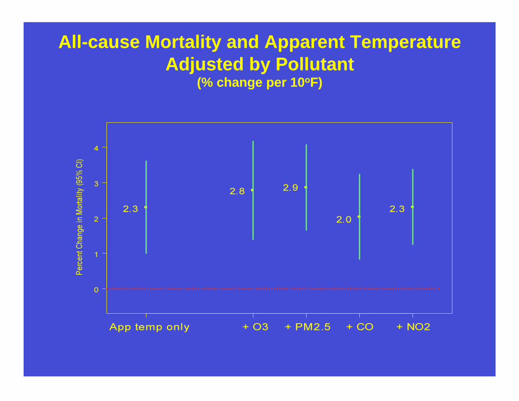
All-cause Mortality and Apparent Temperature

Adjusted by Pollutant (% change per 10oF)

Pooled Results for Apparent Temp:

CA study (% change per 10 o F)

Model Time-Series Case-Crossover

Basic 2.3 (1.0, 3.6) 2.3 (1.0, 3.6)

w. ozone 2.8 (1.3, 4.2)

Match ozone 2.9 (1.8, 4.0)

w. PM2.5 2.9 (1.7, 4.0)

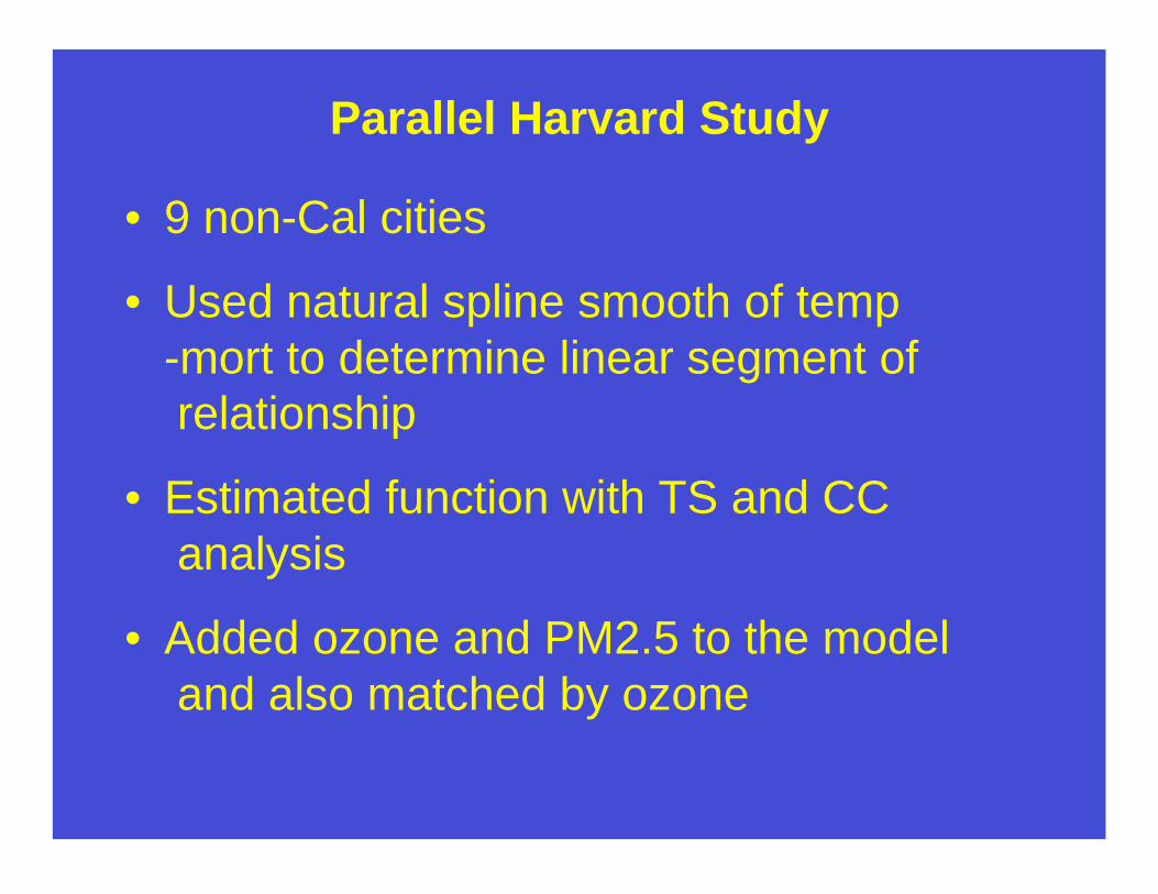
Parallel Harvard Study

• 9 non-Cal cities

• Used natural spline smooth of temp

-mort to determine linear segment of

relationship

• Estimated function with TS and CC

analysis

• Added ozone and PM2.5 to the model

and also matched by ozone

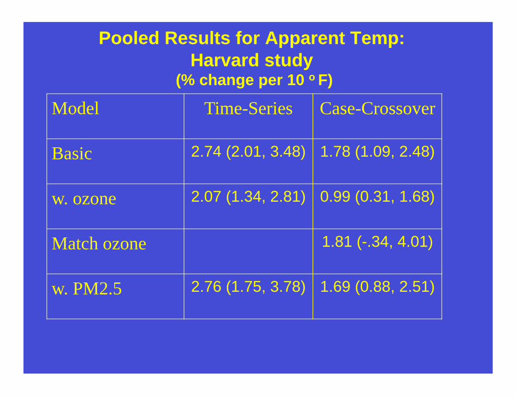
Pooled Results for Apparent Temp:

Harvard study (% change per 10 o F)

Model Time-Series Case-Crossover

Basic 2.74 (2.01, 3.48) 1.78 (1.09, 2.48)

w. ozone 2.07 (1.34, 2.81) 0.99 (0.31, 1.68)

Match ozone 1.81 (-.34, 4.01)

w. PM2.5 2.76 (1.75, 3.78) 1.69 (0.88, 2.51)

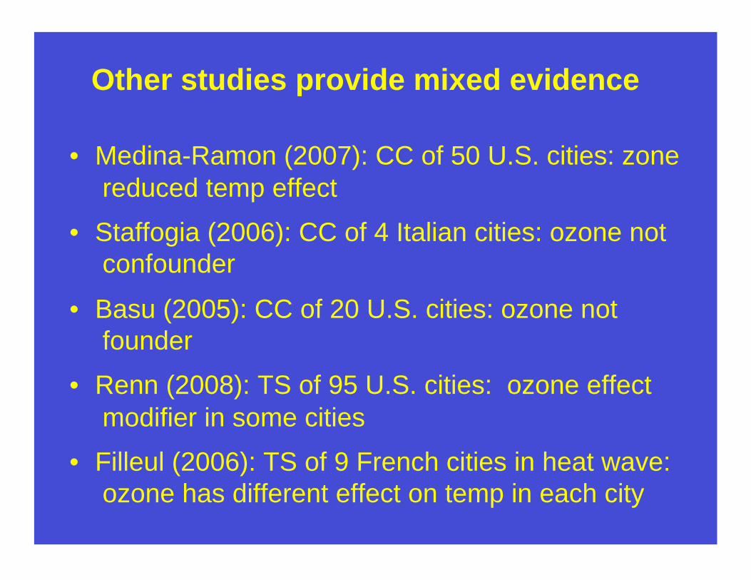
Other studies provide mixed evidence

• Medina-Ramon (2007): CC of 50 U.S. cities: zone

reduced temp effect

• Staffogia (2006): CC of 4 Italian cities: ozone not

confounder

• Basu (2005): CC of 20 U.S. cities: ozone not

founder

• Renn (2008): TS of 95 U.S. cities: ozone effect

modifier in some cities

• Filleul (2006): TS of 9 French cities in heat wave:

ozone has different effect on temp in each city

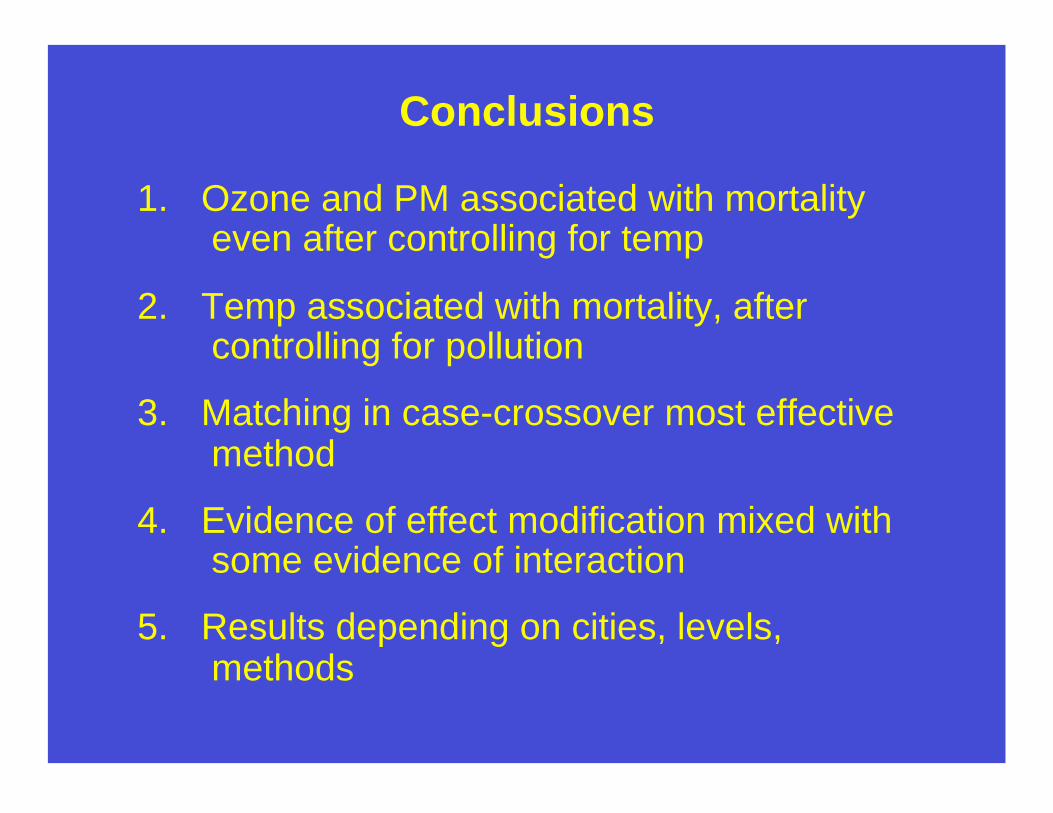
Conclusions

1. Ozone and PM associated with mortality even after controlling for temp

2. Temp associated with mortality, after controlling for pollution

3. Matching in case-crossover most effective method

4. Evidence of effect modification mixed with some evidence of interaction

5. Results depending on cities, levels, methods

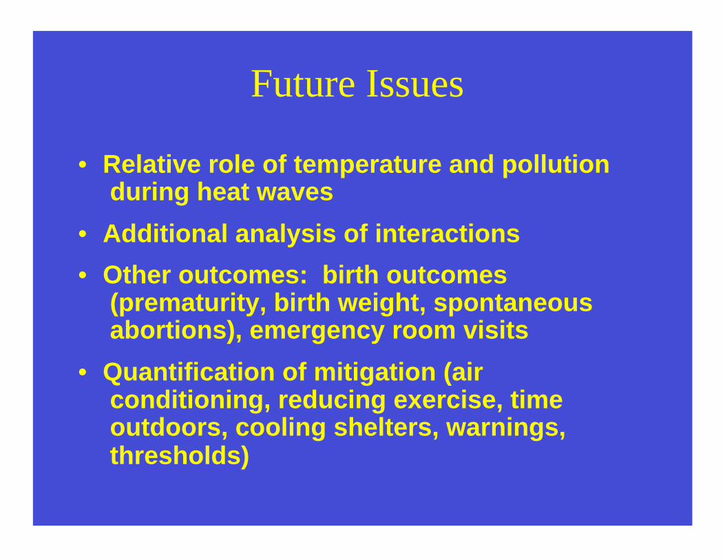
Future Issues

• Relative role of temperature and pollution during heat waves

• Additional analysis of interactions

• Other outcomes: birth outcomes (prematurity, birth weight, spontaneous abortions), emergency room visits

• Quantification of mitigation (air conditioning, reducing exercise, time outdoors, cooling shelters, warnings, thresholds)