Estimating the environmental costs of soil erosion at

multiple scales in Kenya using emergy synthesis

Matthew J. Cohen a,*, Mark T. Brown a, Keith D. Shepherd b

a H.T. Odum Center for Wetlands, Department of Environmental Engineering Sciences, University of Florida,

P.O. Box 116350, Gainesville, FL 32611-6350, USAb World Agroforestry Center/International Center for Research in Agroforestry (ICRAF), United Nations Avenue-Gigiri,

P.O. Box 30677, Nairobi, Kenya GPO 00100

Received 16 September 2004; received in revised form 22 June 2005; accepted 7 October 2005

Available online 15 December 2005

Abstract

The intrinsic value of soil to national, regional and local agroecological and economic productivity in sub-Saharan Africa is not adequately

manifest in financial planning and decision making, challenging long-term sustainability as that resource degrades. While efforts to internalize

the external costs of soil erosion in monetary units are available in the literature, we offer an alternative approach based on emergy synthesis,

which enumerates the value of soil based on the environmental work required to produce it rather than based on surveys or derived pricing

techniques. Emergy synthesis integrates all flows within a system of coupled economic and environmental work in common biophysical units

(embodied solar energy or solar emjoules—sej), facilitating direct comparisons between natural and financial capital. Insight into long-term

sustainability of human economic production and its basis in natural capital stocks is achieved via a suite of emergy-based indices. Our

objective was to provide context for the magnitude of soil erosion losses within the larger resource basis of the Kenyan economy at three

scales. Our results suggest that erosion losses at the national scale (4.5E21 sej/yr) are equal in magnitude to national electricity production or

agricultural exports (equivalent to $ 390 million annually or 3.8% of GDP). This significant hidden, long-term cost is magnified in the selected

district economies. In particular, in Nyando district (a densely populated rural district in western Kenya) we estimate that soil erosion

represents over 14% of total emergy flows. The soil intensity of agriculture (SIA = agricultural yield/soil loss, both in emergy units) of

Nyando (2.25) illustrates a severely marginalized agricultural sector in comparison with the nation as a whole (SIA = 7.56) or other nations

(SIAUSA = 81.9, SIABrazil = 15.6). Soil loss measurements across land uses typical in western Kenya allowed emergy evaluation of differential

costs and benefits; soil loss represented between 12 and 62% of total emergy use (subsistence agriculture SIA = 8.13, communal rangeland

SIA = 1.62). By quantifying the ecological costs of soil erosion in units directly comparable with flows in other sectors of the economic

system, we provide a baseline measure of sustainability against which appropriate investment (i.e., scaled to problem magnitude, targeted to

hot-spots) in soil conservation may be evaluated.

# 2005 Elsevier B.V. All rights reserved.

Keywords: Emergy synthesis; Soil erosion; Kenya; Externality; Natural capital; Systems analysis

www.elsevier.com/locate/agee

Agriculture, Ecosystems and Environment 114 (2006) 249–269

* Corresponding author. Present address: Wetland Biogeochemistry

Laboratory, Soil and Water Science Department, University of Florida,

106 Newell Hall, P.O. Box 1105010, Gainesville, FL 32611-0510, USA.

Tel.: +1 352 392 1804x349; fax: +1 352 392 3399.

E-mail address: mjc@ufl.edu (M.J. Cohen).

0167-8809/$ – see front matter # 2005 Elsevier B.V. All rights reserved.

doi:10.1016/j.agee.2005.10.021

1. Introduction

Soil is functionally a non-renewable resource; while

topsoil develops over centuries, the world’s growing human

population is actively depleting the resource over decades.

As a non-renewable resource and the basis for 97% of all

food production (Pimentel, 1993), strategies to prevent soil

depletion are critical for sustainable development. Sig-

nificant literature exists documenting the magnitude of the

M.J. Cohen et al. / Agriculture, Ecosystems and Environment 114 (2006) 249–269250

soil erosion problem. Between 30 and 50% of the world’s

arable land is substantially impacted by soil loss (Pimentel,

1993), which directly affects rural livelihoods (Lal, 1985;

Kerr, 1997) in addition to indirectly affecting aquatic

resources (Ochumba, 1990; Eggermont and Verschuren,

2003), lake/river sediment dynamics (Kelley and Nater,

2000; Walling, 2000), global carbon cycling (Duxbury,

1995; Lal, 2003), aquatic and terrestrial biodiversity

(Harvey and Pimentel, 1996; Alin et al., 2002) and

ecosystem services (Tinker, 1997; Pimentel and Kounang,

1998). Severe soil degradation has been documented

throughout sub-Saharan Africa (Thomas and Senga, 1983;

Lal, 1985; Pimentel, 1993; Oostwoud and Bryan, 2001;

Lufafa et al., 2002), resulting in declining functional

capacity (Smaling, 1993; Zobisch et al., 1995; Gachene

et al., 1997), ultimately affecting poverty and food security

(Sanchez et al., 1997).

Soil loss has ecological and economic impacts at scales

ranging from the field, where nutrient depletion, degraded

soil structure and lost organic matter affect farm livelihoods

(Morgan, 1995), to the watershed and nation, where

sediment and nutrient loads alter water quality and storage,

and adversely affect ecosystem function (Clark, 1987).

Several studies (Smaling, 1993; Sanchez et al., 1997) have

documented the significance of erosion in soil functional

degradation throughout sub-Saharan Africa at these varied

scales, which, given minimal use of soil amendments by

rural farmers, has profound implications on sustained

regional agricultural production (Lal, 1995). Though some

local success in controlling and reversing soil degradation

has been documented (Tiffen et al., 1994), the soil resource

continues to decline regionally (Sanchez et al., 1997),

alarmingly so in areas (Oostwoud and Bryan, 2001).

The link between soil erosion and agricultural yields has

been widely cited (Lal, 1995; Mulengera and Payton, 1999),

with most attention paid to nutrient limitation. While the

severity of the erosion problem is disputed (Crosson, 1986,

1995; Stocking, 1995), it is clear that agricultural yields in

Africa have failed to match improvements observed

elsewhere (World Bank, 1996), and that a primary constraint

to improved yields is soil nutrition. Erosion affects all

ecosystem services provided by the soil resource (structure,

water holding, carbon storage, etc.) in addition to decreasing

nutrient availability (Zobisch et al., 1995). Without

quantifying the intrinsic value of these services in the

context of the resource basis of the economy, decision

makers have no way to evaluate problem severity, nor any

quantitative rationale to justify diverting sufficient resources

to attenuate it. Indeed, the decision to allocate resources to

protect soil or reverse degradation may be based on

exaggerated claims of severity (Stocking, 1995). Resource

allocations to soil conservation by international agencies

and national governments to date have been substantial

(Kiome and Stocking, 1995) and it must be recognized that

allocating resources to soil conservation requires diversion

from other priorities. Our primary objective is to quantify

erosion costs in direct comparison with other facets of the

internal market economy to better understand the problem

and provide a rationale for effective management decisions.

1.1. Evaluating the costs of soil erosion

The literature is replete with efforts to internalize the

external (i.e., borne by society, now or in the future, rather

than by individuals whose activity engenders the problem—

Loehman and Randhir, 1999; Pretty et al., 2000) costs of

erosion by placing value on eroded soil (Crosson, 1986;

Pimentel et al., 1995; Bojo, 1996; Bandara et al., 2001).

Institutional intervention of some kind is then required to

adjust market prices to reflect true environmental costs.

Most studies focus on links between soil degradation and

productivity, but there is increasing attention to off-site

impacts as concerns about eutrophication and excess

turbidity grow (Clark, 1987; Crul, 1995; Lindenschmidt

et al., 1998). Corollary to the concept of valuing eroded soil

is that some erosion may be tolerable when tradeoffs

necessary to lower loss rates are evaluated (Alfsen et al.,

1996); only by comparing erosion costs with intervention

benefits can effective policy be deduced.

Soil value can be quantified using many techniques. Most

infer value based on market costs of replacing ‘‘free’’

services provided by soils after degradation (e.g. fertilizers,

organic amendments); some equate downstream remedia-

tion costs (e.g., reservoir dredging) with on-site ‘‘external’’

costs (Starett, 2000). Others infer costs based on the value

consumers attach to undegraded lands. Finally, quantifica-

tion of ecological services is often achieved using surveys to

enumerate the ‘‘willingness-to-pay’’ for services provided

by soil (Alfsen et al., 1996). For each, the objective is to

estimate value in units that allow comparison with market

prices.

There have been numerous critiques of economic

valuation of ecological services (e.g. Pritchard et al.,

2000; Ludwig, 2000), despite their obvious attraction from a

practical and regulatory perspective (Hall et al., 2001). One

critique is that methods that assess inherent values of natural

capital contingent on perceived human values may fail to

capture the full extent of ecosystem services. In particular, it

seems realistic to argue that failure by humans to appreciate

the inherent and long-term value of protecting topsoil is a

reason that soil decline continues worldwide and that efforts

are ongoing to artificially internalize those costs in market

decisions.

Methods that complement efforts to quantify the soil

resource value in money units (Bojo, 1996; Kerr, 1997) by

avoiding reliance on human preference may provide an

informative benchmark against which derived monetary

valuation can be compared. Emergy synthesis (Odum,

1996), a technique for valuing environmental work and

natural capital offers several advantages over methods

assigning money values to services for which no market

exists. First, it is based on biophysical processes rather than

M.J. Cohen et al. / Agriculture, Ecosystems and Environment 114 (2006) 249–269 251

derived/perceived human value (e.g., hedonic pricing,

willingness-to-pay), eliminating preference from the valua-

tion schema. Second, allocation of value is donor based,

which frequently simplifies analyses. Value is embodied in

natural capital (e.g., topsoil) predicated on the environ-

mental work required to produce it rather than on services

that stock provides, which are numerous, coupled, indirect

and manifest at varied time and spatial scales, making

boundary definitions and scope difficult to standardize.

1.2. System organization and energetics

Ecological and human systems self-organize to transform

sources of available energy into work (Odum, 1994); as

these transformations occur, a portion of energy previously

available loses its ability to do work, increasing entropy at

the larger scale. However, energy retained after adaptive

transformations has qualities (Odum, 1996) that distinguish

it from the original energy (e.g., the ability to reinforce or

amplify input flows, feedback control). In adaptive systems,

Odum (1996) theorizes that energy is invested in products

only where commensurate feed back control (or ecosystem

service) is provided to enhance overall system function; as a

result, value (in a systems sense) cannot be inferred from

energy content alone, but must account for all investments

required for production, tracing sources back to common

benchmarks to incorporate energy degraded in prior

transformations; this framework is called environmental

accounting.

A donor value accounting framework, wherein value is

derived from biophysical work necessary for production, is

useful for evaluating long-term system sustainability. In

particular, a loss of a natural capital stock (e.g. topsoil) that

has been embedded in a self-organizing system and provides

myriad ecological services is valued according to the

production requirements for replacement. Human activities

that deplete natural capital may have consequences at

multiple scales on and off-site, with inherent time lags and

non-linear responses; to enumerate all ‘‘receiver’’ costs (e.g.

reduced fertility, sedimentation, eutrophication) requires

information that may be difficult to acquire and standardize

between practitioners (Enters, 1997). As such, donor

valuation offers a useful complement to receiver-based

methods for measuring sustainability.

1.3. Emergy synthesis

Emergy is defined as the energy required directly and

indirectly to create a product or service (Odum, 1996; Odum

et al., 2000a). Since each input to a process is itself the

product of energy transformations, emergy is often referred

to as energy memory, with units referenced to a benchmark

energy source (typically solar energy). The emergy unit is

the solar emjoule (sej), indicating that emergy is derived

from energy flows but is qualitatively different; specifically,

emergy accounts for energy degraded (2nd law losses)

during sequential transformations from a benchmark (solar

energy) to other energy forms. Available energy after each

transformation has properties that distinguish it qualitatively

from heat. Energy quality (called transformity; units sej/J or

sej/g) is the ratio of emergy in a product to the remaining

available energy (Odum, 1988).

Transformity values are used to compare process

efficiencies (inputs versus outputs) for industrial (Brown

and Buranakarn, 2003; Ulgiati and Brown, 1998), agricul-

tural (Ulgiati et al., 1994; Lagerberg, 1999; Brandt-

Williams, 2001; Doherty et al., 2002) and forestry (Doherty

et al., 2002) systems. They allow direct comparison of

biophysical flows in common units; evaluations that ignore

energy quality undervalue contributions of small concen-

trated flows (e.g., human work, top-carnivores) relative to

abundant diffuse ones (e.g., sunlight, primary production)

(Christensen, 1994). Numerous studies have used emergy

synthesis to quantify development tradeoffs that consider

both economic and ecological costs and benefits (Brown and

McClanahan, 1996; Alejandro Prado-Jatar and Brown,

1997; Portela, 1999; Odum et al., 2000b; Buenfil, 2001).

Evaluations have focused on water (Romitelli, 1997; Brandt-

Willams, 1999; Howington, 1999), forest products (Doherty

et al., 2002), and multi-use forest functions (Tilley and

Swank, 2003).

We use emergy synthesis to evaluate soil loss at three

scales in Kenya. Dramatically accelerated soil loss is widely

observed throughout Kenya, particularly in western districts

where high rural population densities, intense climatic

inputs and fragile soils converge. Nationally, erosion is

estimated between 25 and 180 million tonnes of soil loss

annually (Barber, 1983; Smaling, 1993). Our objective is to

place this flow in a quantitative framework that includes

other aspects of the economic/environment system for direct

comparability, reasoning that a clearer understanding of the

problem magnitude will elicit the investments necessary for

attenuation.

2. Study area—the Kenyan system

Kenya lies in equatorial East Africa, bordered by

Tanzania, Uganda, Sudan, Ethiopia and Somalia (Fig. 1).

Diverse climates (extreme aridity to montane rainforest),

elevations (0–5500 m), cultural groups (Bantu, Nilotic,

Arab, Asian, Caucasian and Khoi-San) and livelihood

strategies persist in this small nation (580,000 km2). Kenya

has high population growth rates (>3% per year in the

1980’s, now 1–2%, in part due to the effects of HIV) and is

home to 31 million people. Political stability, market

capitalism, coastal access, a well-educated population, and a

lucrative tourism industry have elevated economic condi-

tions in Kenya above those typical of the region, though the

national economy shrank on a per capita basis in recent years

(World Bank, 2002). GDP in 2001 was $ 10.2 billion,

corresponding to $ 330 per capita, placing Kenya among the

M.J. Cohen et al. / Agriculture, Ecosystems and Environment 114 (2006) 249–269252

Fig. 1. Map of Kenya, Kisumu, Nyando and Kericho Districts and Nyando River basin. Also shown is national elevation map, Lake Victoria and Kenya’s major

urban centers.

poorer countries (global �$ 5000/capita). International debt

is significant; Kenya owes over $ 6 billion (World Bank,

2002) resulting in annual service of 25% of export revenue.

Major imports include fuels, fertilizers, metals and

machinery (UN 2000). Major exports include agricultural

products (�50%, sugar, coffee, tea, pyrethrum, tobacco, cut

flowers and sisal), and manufacturing (�20%, petroleum/

food processing, engineering services, textiles). Roughly

90% of the population relies on subsistence cropping and

animal husbandry. Since only �7% of the land is arable,

rural population densities can exceed 500 km�2. Kenya’s

major rivers (Mara, Tana, Athi, Nyando, Sondu, Yala-Nzoia)

deliver an estimated 313 t/km2/yr of sediment to Lake

Victoria and the Indian Ocean (Ministry of Water

Development, 1992; FAO, 2001). While land tenure

conditions are generally favorable, agricultural extensifica-

tion has forced cultivation of marginal lands (low rainfall,

infertile, steep slopes) and illegal clearing of protected

forests (forests cover �3% of area; loss rate �1.4%/yr).

Kenya’s reliance on natural capital includes ecotourism

revenue; 700,000 tourists visit Kenya annually, yielding US$

470 million in 1999.

2.1. Nyando River basin

Conditions of rural poverty are acutely evident in western

Kenya where rural population densities are among the

highest in Africa, and soil degradation is both prevalent and

severe. The political districts (Kisumu, Nyando and

Kericho) comprising the Nyando basin (Fig. 1) and regional

land use subsystems therein are focal points of this work;

this basin has been identified as a regional erosion hot-spot

(ICRAF, 2000). The Nyando River drains the western

highlands, dropping from 3000 m to Lake Victoria (Nyanza

Gulf) at 1184 m. The basin is divided into lowlands

(<1500 m) and highlands (>1500 m), separated by a steep

escarpment. Lowland climate is sub-humid tropical

(�1100 mm rain/yr) with bi-modal rainfall characteristic

of equatorial latitudes. Highland climate is humid tropical

(�1700 mm rain/yr) exhibiting moderated bi-modal rainfall

due to subsidized convection from Lake Victoria; annual

insolation and temperature are constant. Lowlands consist

primarily of Pleistocene lake plain deposits (Planisols and

Vertisols) with deep profiles and moderate to low fertility.

Highland soils are deeply weathered (Nitisols, Cambisols)

M.J. Cohen et al. / Agriculture, Ecosystems and Environment 114 (2006) 249–269 253

and structurally stable. Dominant lowland agricultural land

uses are maize, sugarcane and communal rangeland, while

tea, maize, commercial woodlots and paddock grazing (with

improved breeds) dominate the highlands. Native ecological

communities, now rare, include perennial grasslands in the

lowlands, and evergreen broadleaf forest in the highlands.

Erosion is particularly severe in the lowlands where, despite

shallow relief, networks of gullies and eroded riverbanks

threaten transportation, agricultural production, settlements,

and downstream water quality. Severe soil crusting is

prevalent. Soil degradation prevalence (55% of lands

degraded, 25% severely) was estimated by linking ground

survey data with satellite imagery in the Awach River basin,

a major tributary of the Nyando (Cohen et al., 2005).

3. Methods

Emergy synthesis was applied to economic/environ-

mental systems at three scales in Kenya, starting from the

largest scale and focusing on increasingly local systems.

1. A

national scale evaluation was developed to quantify the

significance of soil degradation to the national economy

and provide context for evaluations at smaller scales.

2. T

hree districts (3rd level of the Kenyan government) in

the western region of Kenya that coincide with the

Nyando River basin (a hot-spot for erosion, Fig. 1) were

evaluated.

3. L

and uses that are the primary rural livelihood strategies

comprised the local scale. Commercial agriculture (sugar

and tea), subsistence agriculture (maize), fuel/timber

woodlots, grazing lands, and forests/shrublands

(exploited for fuelwood) were examined.

Emergy synthesis of nations, regions and land uses (all on

an annual basis) has been standardized to convey general-

ized information about the energy basis for economic and

environmental condition (Ulgiati et al., 1994; Odum, 1996;

Doherty et al., 2002); this standard template, with five

analytical steps, was followed at each scale (see Doherty

et al., 2002 for details):

1. C

ompilation of cross-boundary flows, internal transfor-

mations (environmental and economic) and stock

depletion (mining, erosion, forest loss)—this exercise

summarizes literature sources (e.g. development reports,

economic abstracts, environmental abstracts).

2. S

ystems diagram development—use the energy sys-

tems language (defined in supporting materials) to

depict the resource basis. Conventions are given in

Odum (1994).

3. D

ata collection—identify data sources for cross-bound-

ary flows and internal natural capital depletion rates.

Summarize economic/environmental production and

trade data.

4. T

abular assessment—a standard accounting framework is

applied wherein each resource flow is evaluated in

physical units, modified by an appropriate transformity to

adjust for energy quality (to allow direct comparison

between flows of different physical form).

5. F

low aggregation/ index development—summary

indices have been developed (Ulgiati et al., 1994) to

capture various aspects of environment/economy inter-

actions.

3.1. Emergy tables

Standard analysis templates have been developed to

expedite data handling and flow aggregation (Ulgiati et al.,

1994; Stachetti unpublished template). Tables consist of

named flows (identified as necessary during diagram

development), physical units of flow (J, g, $), transformity

values that translate physical units into emergy (sej), and

total emergy. Since flows are reported on an annual basis,

total emergy is expressed in units of sej/yr. A final column in

a standard table provides an indirect link with economic

measures of value. The macroeconomic value of each flow is

reported in equivalent $ (referred to as Em$ to avoid

confusion). This value is the emergy flow for each source

divided by the emergy money ratio (EMR—see below).

3.2. Transformity values

Transformities specific to Kenya were used where

possible, but in most cases previously computed values

were used. For Kenya’s major agricultural products (n = 17),

transformities were computed using a standard analysis

frame (Brandt-Williams, 2001), linking detailed agroeco-

logical inventory and yield data (Jaetzold and Schmidt,

1982) with soil loss estimates (Barber, 1983; Cohen, 2003)

and climatological input data (Corbett et al., 1997). These

products included raw goods (e.g. maize, sorghum, tea,

sugar cane, tobacco), protein sources (fish, cattle) and

processed goods (tea and sugar). Transformity values used

are given in supporting materials.

Using an appropriate transformity for topsoil was

paramount—previous values (1.1E+05 sej/J, Odum, 1996)

are based on soil organic matter (SOM) turnover rates for

temperate regions where SOM accumulation is more rapid

than in the sub-humid seasonal tropics (Nye and Greenland,

1960; Coleman et al., 1989). We estimated emergy

requirements for SOM production in two tropical systems

(savannah and forest) to determine a more appropriate

transformity for the region. Typically, SOM is the ‘‘value-

bearer’’ for soil; other functional attributes are subsumed

under that component. The rationale for this assumption is

that all aspects of soil development (physical, chemical and

biological) are coupled, and counting each as a separate cost

would ‘‘double-count’’ the emergy required for their parallel

production.

M.J. Cohen et al. / Agriculture, Ecosystems and Environment 114 (2006) 249–269254

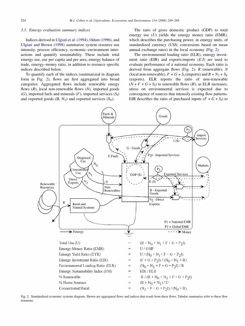
3.3. Emergy evaluation summary indices

Indices derived in Ulgiati et al. (1994), Odum (1996), and

Ulgiati and Brown (1998) summarize system resource use

intensity, process efficiency, economic–environment inter-

actions and quantify sustainability. These include total

emergy use, use per capita and per area, emergy balance of

trade, emergy–money ratio, in addition to resource specific

indices described below.

To quantify each of the indices (summarized in diagram

form in Fig. 2), flows are first aggregated into broad

categories. Aggregated flows include renewable energy

flows (R), local non-renewable flows (N), imported goods

(G), imported fuels and minerals (F), imported services (SI)

and exported goods (B, N2) and exported services (SE).

Fig. 2. Standardized economic systems diagram. Shown are aggregated flows and

notations.

The ratio of gross domestic product (GDP) to total

emergy use (U) yields the emergy money ratio (EMR),

which describes the purchasing power, in emergy units, of

standardized currency (US$; conversions based on mean

annual exchange rates) in the local economy (Fig. 2).

The environmental loading ratio (ELR), emergy invest-

ment ratio (EIR) and exports:imports (E:I) are used to

evaluate performance of a national economy. Each ratio is

derived from aggregate flows (Fig. 2): R (renewable), N

(local non-renewable), F + G + SI (imports) and B + N2 + SE

(exports). ELR reports the ratio of non-renewable

(N + F + G + SI) to renewable flows (R); as ELR increases,

stress on environmental services is expected due to

convergence of sources that intensify existing flow patterns.

EIR describes the ratio of purchased inputs (F + G + SI) to

indices that result from these flows. Tabular summaries refer to these flow

M.J. Cohen et al. / Agriculture, Ecosystems and Environment 114 (2006) 249–269 255

total internal flows (N + R), and quantifies outside invest-

ment to match flows of locally available emergy (i.e.,

attraction potential). Large EIR values indicate advanced

regional or national development; EIR for the USA is 7:1

(Odum, 1996), and 0.46:1 for Thailand (Brown and

McClanahan, 1996). E:I quantifies the net trade benefit

for a nation or region. Values below 1 indicate net imports,

generally associated with advanced development (Odum,

1996). The emergy sustainability index (ESI, Brown and

Ulgiati, 1999) is the ratio of EIR to ELR; sustainability (ESI)

increases with investment (EIR—to remain competitive) and

decreases with environmental load (ELR). At the land use

subsystem scale, we use the emergy yield ratio (EYR = Y/F)

as a measure of return-on-investment in units of environ-

mental work.

3.4. Soil loss indices

Two new metrics were developed specifically to

quantify losses of stocks of soil natural capital within

the context of a regional energy basis. Typically, soil loss is

considered non-renewable energy stock depletion (N in

Fig. 3). However, grouping these flows with mined

minerals and locally extracted fossil fuels ignores direct

ecosystem services that these stocks facilitate. Further-

more, while direct economic benefits of fuel extraction or

mineral mining are clear, the benefit of degraded topsoil is

Fig. 3. Simplified schemat

not as obvious. It is reasonable to assume that at least a

portion of these flows could be prevented given more

effective land management policies.

The first new index scales soil loss to the emergy basis for

the regional system. The fraction of use soil erosion (FUSE)

is computed as % of total use (U) arising from erosion (N0a):

FUSE ¼ N0a

U(1)

The second new index provides a cost-benefit ratio for

agriculture. The soil intensity of agriculture (SIA) compares

agricultural yields (livestock and crops) to the emergy in

eroded soil:

SIA ¼ Yag

N0a

(2)

where Yag is the emergy yield from agriculture. Because

erosion is embodied as a component of agricultural yields

(i.e., soil loss is in both the numerator and denominator), the

index minimum is one; values near one indicate strongly

deleterious agricultural effects. Large FUSE values indicate

substantial external costs to the economy. Both FUSE and

SIA are independent of other standard regional analysis

indices, and can be computed for all nations for which

emergy evaluations have been done for comparative pur-

poses. SIA should vary considerably within and between

regions and cropping systems, identifying agricultural and/

ic of topsoil genesis.

M.J. Cohen et al. / Agriculture, Ecosystems and Environment 114 (2006) 249–269256

or livestock activities are locally inappropriate. Note that, at

the land use scale, SIA is inverse of FUSE; this is not the

case at larger scales where total use (U) is not exclusively

due to agriculture.

3.5. Data sources—national scale

Renewable flow data were compiled from existing and

derived data. Insolation and mean tidal range/wave height

were all assumed uniform over area and coastline,

respectively (US Dept. of Commerce-NOAA, 1994).

Existing thematic coverages were used for elevation

(Fig. 1), precipitation and land use (Corbett et al., 1997);

thematic layers interpolated from point coverages were

developed for deep heat (data from Pollack et al., 1993) and

wind (Chipeta, 1976).

Production, consumption and trade data were readily

available at the national scale. Internal and cross-boundary

flows were obtained primarily from a national statistical

abstract published by the Kenyan Central Bureau of

Statistics (KCBS, 2000), which compiled national accounts

from 1999. Numerous ancillary data sources were used, both

to quantify flows not available from the statistical abstract

and to cross-reference flows to ensure accurate accounting.

These sources included United Nations commodity flow

data (FAO-UN, 1999), Europa World Yearbook (Europa

Publications, 2000), International Trade Statistics Yearbook

(UN Dept. of Economic and Social Affairs, 2000), and a

World Bank national overview (World Bank, 2002).

Internal agricultural/fisheries/livestock production,

geothermal and hydroelectric power production, forest

clearing rates and mining data were all compiled from

both published (e.g. Rural Planning Department, 1997a,b,c)

and Government of Kenya (GoK) publications, including the

Ministry of Agriculture and Rural Development (MoARD),

Kenya Pipeline Authority (KPA—parastatal agency respon-

sible for fuel refining, transport and sale), Ministry of

Fisheries, Kenya Power and Lighting Corporation (KPLC),

Ministry of Forestry and Bureau of Mines.

3.6. National soil loss estimation

Two methods were used to estimate annual soil loss

quantities: (1) use of soil loss rates on a land use basis

(Barber, 1983), adjusted by a sediment delivery ratio (FAO,

2001; Ministry of Water Development, 1992; Brooks et al.,

1997); (2) measurements of sediment concentration in rivers

(Ministry of Water Development, 1992). Typically, the latter

would be considered more reliable for cross-boundary flows,

but available data are from the 1970s and cover a very

limited number of rivers. Therefore, the first method was

used, with the second providing a cross-check.

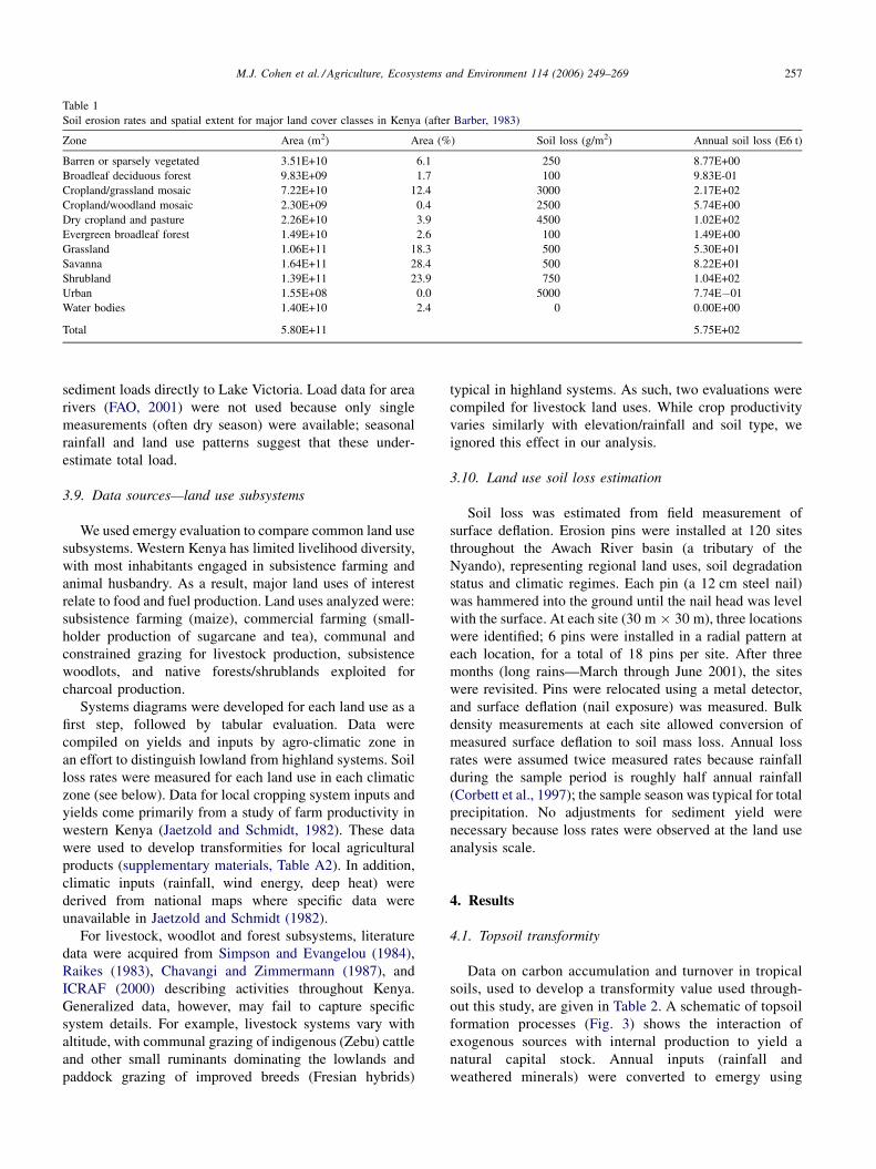
Average annual soil loss rates by land use (Table 1) were

multiplied by areas inferred from national land use maps

(Corbett et al., 1997). Soil loss estimates were multiplied by

a sediment yield ratio (assumed 5%, Brooks et al., 1997) to

avoid including eroded material subsequently deposited

downstream (wetlands, concave slopes, etc.). This approach

is conservative with regard to real soil degradation costs

because material eroded and deposited downstream is

assumed to represent zero cost. Since sedimentation in

waterways is detrimental to ecosystem processes, it might

constitute a substantial additional receiver cost (Crul, 1995).

Forest clearing at the national scale was quantified using a

clearing rate of 1.25% per year; Kaufman et al. (1996)

estimate clearing rates between 1 and 1.7% per year for the

last several decades. Biomass loss through clearing was

assumed to be 80 t/ha/yr.

3.7. Data sources—district scale

Renewable flows were derived from national maps. Local

non-renewable and trade flows at the district level were

acquired from several sources. District development plans

(Rural Planning Department, 1997a,b,c) report on climate

and agricultural production, demographics and development

indicators. Resource consumption and trade between regions

for some flows were obtained from parastatal agencies,

including electricity consumption (Kenya Power and

Lighting Corporation), fuel distribution/refining (Kenya

Pipeline Authority) and tea/sugar production (Kenya Tea

Development Authority; Kenya Sugar Authority).

Records of manufacturing, mining, services and trans-

portation are not collected, and the limited data were judged

suspect. To estimate flows of manufactured commodities

(e.g. metals, services, textiles) that are not documented by

reliable sources at the district scale, it was assumed that

consumption is proportional to utilization of fuels and

electricity, using the national analysis as the proportional

reference point. Cleveland et al. (1984) found that economic

flows are highly correlated with fuel/energy use, supporting

this assumption. Each derived flow is computed as:

Fi; j ¼ Fi;n �R j

RN(3)

where Fi,j is a derived flow for resource i, for district j. The

subscript N refers to the flow of the same resource at the

national scale. Flows RN and Rj are the flows of fuel and

electricity at the national and district scale, respectively. A

strong proportionality relationship between fuel use, elec-

tricity use and economic product was observed between the

national and district figures.

3.8. District soil loss estimation

Soil loss at the district scale was estimated from field

measurements of loss rates for each land use coupled with

land use maps. A sediment yield ratio (sediment load:ero-

sion) of 10% was assumed because this region is dominated

by small basins, which typically exhibit high yields (Brooks

et al., 1997). In particular, significant drainage occurs via

small ungauged escarpment streams discharging large

M.J. Cohen et al. / Agriculture, Ecosystems and Environment 114 (2006) 249–269 257

Table 1

Soil erosion rates and spatial extent for major land cover classes in Kenya (after Barber, 1983)

Zone Area (m2) Area (%) Soil loss (g/m2) Annual soil loss (E6 t)

Barren or sparsely vegetated 3.51E+10 6.1 250 8.77E+00

Broadleaf deciduous forest 9.83E+09 1.7 100 9.83E-01

Cropland/grassland mosaic 7.22E+10 12.4 3000 2.17E+02

Cropland/woodland mosaic 2.30E+09 0.4 2500 5.74E+00

Dry cropland and pasture 2.26E+10 3.9 4500 1.02E+02

Evergreen broadleaf forest 1.49E+10 2.6 100 1.49E+00

Grassland 1.06E+11 18.3 500 5.30E+01

Savanna 1.64E+11 28.4 500 8.22E+01

Shrubland 1.39E+11 23.9 750 1.04E+02

Urban 1.55E+08 0.0 5000 7.74E�01

Water bodies 1.40E+10 2.4 0 0.00E+00

Total 5.80E+11 5.75E+02

sediment loads directly to Lake Victoria. Load data for area

rivers (FAO, 2001) were not used because only single

measurements (often dry season) were available; seasonal

rainfall and land use patterns suggest that these under-

estimate total load.

3.9. Data sources—land use subsystems

We used emergy evaluation to compare common land use

subsystems. Western Kenya has limited livelihood diversity,

with most inhabitants engaged in subsistence farming and

animal husbandry. As a result, major land uses of interest

relate to food and fuel production. Land uses analyzed were:

subsistence farming (maize), commercial farming (small-

holder production of sugarcane and tea), communal and

constrained grazing for livestock production, subsistence

woodlots, and native forests/shrublands exploited for

charcoal production.

Systems diagrams were developed for each land use as a

first step, followed by tabular evaluation. Data were

compiled on yields and inputs by agro-climatic zone in

an effort to distinguish lowland from highland systems. Soil

loss rates were measured for each land use in each climatic

zone (see below). Data for local cropping system inputs and

yields come primarily from a study of farm productivity in

western Kenya (Jaetzold and Schmidt, 1982). These data

were used to develop transformities for local agricultural

products (supplementary materials, Table A2). In addition,

climatic inputs (rainfall, wind energy, deep heat) were

derived from national maps where specific data were

unavailable in Jaetzold and Schmidt (1982).

For livestock, woodlot and forest subsystems, literature

data were acquired from Simpson and Evangelou (1984),

Raikes (1983), Chavangi and Zimmermann (1987), and

ICRAF (2000) describing activities throughout Kenya.

Generalized data, however, may fail to capture specific

system details. For example, livestock systems vary with

altitude, with communal grazing of indigenous (Zebu) cattle

and other small ruminants dominating the lowlands and

paddock grazing of improved breeds (Fresian hybrids)

typical in highland systems. As such, two evaluations were

compiled for livestock land uses. While crop productivity

varies similarly with elevation/rainfall and soil type, we

ignored this effect in our analysis.

3.10. Land use soil loss estimation

Soil loss was estimated from field measurement of

surface deflation. Erosion pins were installed at 120 sites

throughout the Awach River basin (a tributary of the

Nyando), representing regional land uses, soil degradation

status and climatic regimes. Each pin (a 12 cm steel nail)

was hammered into the ground until the nail head was level

with the surface. At each site (30 m � 30 m), three locations

were identified; 6 pins were installed in a radial pattern at

each location, for a total of 18 pins per site. After three

months (long rains—March through June 2001), the sites

were revisited. Pins were relocated using a metal detector,

and surface deflation (nail exposure) was measured. Bulk

density measurements at each site allowed conversion of

measured surface deflation to soil mass loss. Annual loss

rates were assumed twice measured rates because rainfall

during the sample period is roughly half annual rainfall

(Corbett et al., 1997); the sample season was typical for total

precipitation. No adjustments for sediment yield were

necessary because loss rates were observed at the land use

analysis scale.

4. Results

4.1. Topsoil transformity

Data on carbon accumulation and turnover in tropical

soils, used to develop a transformity value used through-

out this study, are given in Table 2. A schematic of topsoil

formation processes (Fig. 3) shows the interaction of

exogenous sources with internal production to yield a

natural capital stock. Annual inputs (rainfall and

weathered minerals) were converted to emergy using

M.J. Cohen et al. / Agriculture, Ecosystems and Environment 114 (2006) 249–269258

Table 2

Annual emergy inputs to ecosystem processes (biomass production, organic matter accumulation)

Note Savanna ecosystem flows Physical flows (units/yr) Units Transformity (sej/unit) Emergy (sej/yr)

1 Sunlight 7.66E+08 J 1 7.66E+08

2 Rainfall 7.50E+06 J 31000 2.33E+11

3 Weathering 60 g 1.70E+09 1.02E+11

Total 3.35E+11

4 Net primary production 1.00E+07 J 3.34E+04

5 OM production 1.76E+06 J 1.91E+05

Note Forest ecosystem flows Physical flows (units/yr) Units Transformity (sej/unit) Emergy (sej/yr)

1 Sunlight 7.66E+08 J 1 7.66E+08

2 Rainfall 1.10E+07 J 31000 3.41E+11

3 Weathering 80 g 1.70E+09 1.36E+11

Total 4.77E+11

4 Net primary production 1.42E+07 J 3.36E+04

5 OM production 2.49E+06 J 1.92E+05

Notes: (1) insolation is assumed equal between systems at 1.83 kcal/m2/yr (FAO, 2001); (2) mean rainfall is 2.2 and 1.5 m/yr for forested and savanna systems,

respectively; (3) mean weathering rates are assumed to be equal to steady state erosion rates of 60 and 80 g/m2/yr for savanna and forest systems, respectively;

(4) net primary production rates (Young, 1976) are 850 and 600 g/m2/yr for forest and savanna systems, respectively. Energy content is assumed 4 kcal/g; (5)

nominal SOM accumulation rates (Nye and Greenland, 1960; Coleman et al., 1989; Parton et al., 1994) are 170 and 120 g/m2/yr for forest and savanna systems,

respectively. Energy content is assumed 3.5 kcal/g.

Fig. 4. Detailed systems diagram of the Kenyan national system (ca. 1999).

M.J. Cohen et al. / Agriculture, Ecosystems and Environment 114 (2006) 249–269 259

Table 3

Emergy evaluation of resource basis for Kenya (ca. 1999)a

Note Item Physical flow Units Transformity

(sej/unit)b

Solar emergy

(E20 sej)

EmDollars

(E9 1999 US$)

Renewable resources

1 Sunlight 3.70E+21 J 1 36.96 0.32

2 Evapotranspiration, chemical 1.68E+18 J 31000 519.65 4.46

3 Runoff, geopotential 3.08E+17 J 47000 144.57 1.24

4 Wind, kinetic energy 3.39E+18 J 2450 83.08 0.71

5 Waves 3.34E+17 J 51000 170.49 1.46

6 Tide 5.49E+17 J 73600 404.24 3.45

7 Earth cycle 1.05E+18 J 58000 609.47 5.21

Indigenous production

8 Hydroelectricity 1.12E+16 J 2.77E+05 31.14 0.27

9 Geothermal electricity 2.25E+15 J 2.69E+05 6.05 0.05

10 Agriculture productionc 1.62E+17 J 8.84E+04 143.21 1.22

11 Livestock productionc 1.31E+16 J 1.11E+06 145.42 1.24

12 Fisheries production 7.47E+14 J 9.42E+06 70.38 0.60

13 Fuelwood production 1.72E+17 J 3.09E+04 53.10 0.45

Local non-renewable sources

14 Const. mater. (sand, ballast) 3.69E+12 g 1.69E+09 62.36 0.53

15 Soda ash 5.81E+11 g 1.69E+09 9.82 0.08

16 Fluorspar, salt, limestone 1.72E+11 g 1.69E+09 2.90 0.02

17 Gold 9.90E+05 g 2.00E+13 0.20 0.00

18 Precious/semi-precious gems 4.30E+07 g 1.00E+13 4.30 0.04

19 Forest clearing 6.18E+16 g 6.72E+04 41.53 0.35

20 Top soil (OM) 2.35E+16 J 1.92E+05 45.18 0.39

Imports

21 Oil derived products 1.41E+17 J 135.45 1.16

Crude petroleum 8.20E+16 J 8.90E+04 72.98

Refined petroleum 5.80E+16 J 1.06E+05 61.41

Petroleum products 1.00E+15 J 1.06E+05 1.06

22 Metals 4.33E+11 g 29.74 0.25

Ferrous metals raw 3.94E+11 2.99E+09 11.79

Non-ferrous metals 2.50E+10 2.69E+10 6.72

Metal structures and tools 1.39E+10 8.06E+10 11.23

23 Minerals 6.87E+10 g 1.16 0.01

Cement 3.94E+10 1.73E+09 0.68

Clay 1.68E+10 2.86E+09 0.48

Glass 1.24E+10 1.08E+07 0.00

24 Food and agricultural productsc 1.48E+16 J 1.44E+05 21.36 0.18

25 Livestock, meat, fishc 1.27E+14 J 4.20E+06 5.33 0.05

26 Plastics and rubber 1.19E+11 g 9.51 0.08

Rubber 1.19E+11 g 7.22E+09 8.59

Plastics 1.45E+11 g 6.38E+08 0.92

27 Chemicals 5.31E+11 g 28.23 0.24

Chemical products, dyes, etc. 1.44E+11 6.38E+08 0.92

Fertilizers 3.87E+11 7.06E+09 27.31

28 Wood, paper, textiles 1.69E+15 J 28.33 0.24

Wood 3.25E+14 3.09E+04 0.10

Paper 9.79E+14 3.61E+05 3.54

Textiles 3.87E+14 6.38E+06 24.69

29 Mechanical and transportation equipment 4.45E+10 g 1.13E+11 50.07 0.43

30 Service in imports 2.75E+09 $ 2.08E+12 57.28 0.49

Exports

31 Food and agricultural productsc 1.32E+16 J 3.77E+05 49.72 0.42

32 Livestock, meat, fishc 4.66E+14 J 3.30E+06 15.40 0.13

33 Wood, paper, textiles 4.87E+15 J 33.22 0.28

Wood 4.15E+15 1.43E+05 5.91

Paper 4.01E+14 3.61E+05 1.45

Textiles 2.57E+14 6.38E+06 16.43

Leather 6.53E+13 1.44E+07 9.43

34 Oil derived products 1.20E+16 J 1.06E+05 12.69 0.11

35 Metals 1.81E+11 g 21.20 0.18

M.J. Cohen et al. / Agriculture, Ecosystems and Environment 114 (2006) 249–269260

Table 3 (Continued )

Note Item Physical flow Units Transformity

(sej/unit)b

Solar emergy

(E20 sej)

EmDollars

(E9 1999 US$)

Ferrous metals 1.67E+11 g 2.99E+09 5.01

Non-ferrous metals 2.57E+09 g 2.69E+10 0.69

Metal structures and tools 1.14E+10 g 1.35E+11 15.50

36 Minerals 7.16E+11 g 16.44 0.14

Cement 6.90E+11 g 1.73E+09 11.94

Glass 2.59E+10 g 1.08E+07 0.00

Gold and gems 4.40E+07 g 1.02E+13 4.49

37 Chemicals 7.90E+10 g 6.38E+08 0.50 0.00

38 Mechanical and transportation equipment 1.48E+09 g 1.13E+11 1.67 0.01

39 Plastics and rubber 5.30E+10 g 0.68 0.01

Plastics 4.78E+10 g 6.38E+08 0.30

Rubber 5.26E+09 g 7.22E+09 0.38

40 Service in exports 1.98E+09 $ 1.17E+13 231.14 1.98

41 Tourism 4.74E+08 $ 1.17E+13 55.46 0.47

a Table footnotes, and raw data/transformity sources are in supplementary information (Table A3).b Transformity values are summarized in supplementary information (Table A1).c Each agricultural and livestock entry aggregates products with differing transformities. The transformity used in each case is a weighted average

transformity across all commodities that comprise the physical flow. Transformities for agricultural products for Kenya are summarized in supplementary

materials (Table A2).

their respective transformity values, then summed. The

emergy driving OM production at the ecosystem scale was

divided by the available energy (assuming 3.5 kcal/g) to

yield a transformity value; a similar calculation was

developed for annual biomass production. The resulting

topsoil organic matter transformity is the same for both

ecosystems (1.92E5 sej/J) as a result of larger exogenous

inputs as well as increased SOM production for forest

production.

4.2. National analysis

4.2.1. Systems diagram

A diagram of the Kenyan environmental/economic

system (Fig. 4) depicts resource flows entering the system

and the organization of major internal components that

utilize those resources. Primary renewable flows are

sunlight, rainfall, and earth heat; purchased goods, fuels,

and services are also shown. Internal production systems

include forests and savannas, commercial and subsistence

farming, rangelands, wetlands and coral reefs; livestock,

fisheries, and native fauna are shown. In addition to direct

extraction from these sectors, associated costs of soil erosion

are depicted (S in each production system represents soil),

along with consequent impacts on aquatic resources. Major

manufacturing sectors include agricultural processing, metal

and mineral processing, and leather and textiles. With

tourism, these are the main revenue generators; the diagram

shows how revenue is generated and spent importing goods

and services from the global market. Purchased sources are

aggregated to avoid excessive complexity, but were

analyzed in detail (Table 3). Government’s role in protecting

wildlife, providing services to urban and rural populations

and managing loans (principal—P and interest—I) is shown.

4.2.2. Emergy table

Detailed tabular accounting of Kenya’s emergy basis

(Table 3, 1999) enumerates renewable resources, indigenous

production, local non-renewable resource extraction,

imports and exports. Sunlight represents 99.8% of total

energy inflow, but only 1.25% of emergy flow (adjusted for

energy quality). Conversely, flows of high quality inputs

(fuels, services, materials) are energetically insignificant

(�0.00001% of total energy), but clearly critical to the

Kenyan system, representing over 35% of total use when

adjusted for quality. In emergy units, the largest renewable

driving the Kenyan economy is rainfall, and to avoid double

counting emergy delivered from coupled processes, only this

flow (rainfall chemical potential + geopotential) is included

in subsequent calculations for R (Odum et al., 2000a).

Most indigenous production is from agriculture and

livestock, followed by managed forest and fishery yields.

Kenya’s electricity (geothermal and hydroelectric) is minor

in comparison, illustrating limited national electrification.

Overall, agriculture and livestock production contribute

1.43E22 and 1.45E22 sej per year. Local non-renewable

flows include mining products (mainly ballast materials),

forest loss (Item 19) and erosion (Item 20).

All fossil fuel resources are imported; other major

imports are embodied services and mechanical/transporta-

tion equipment. Major exports are food and agricultural

products, wood/ paper/textile products and embodied

services (i.e. services that are necessary both directly and

indirectly to facilitate exports, quantified using money

received multiplied by the Kenyan EMR).

4.2.3. Flow aggregation

Flow aggregations (Table 4) include renewable, local

non-renewable, imports and exports. Also included are

M.J. Cohen et al. / Agriculture, Ecosystems and Environment 114 (2006) 249–269 261

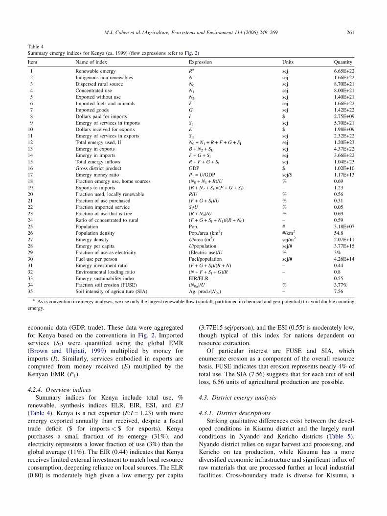
Table 4

Summary emergy indices for Kenya (ca. 1999) (flow expressions refer to Fig. 2)

Item Name of index Expression Units Quantity

1 Renewable emergy Ra sej 6.65E+22

2 Indigenous non-renewables N sej 1.66E+22

3 Dispersed rural source N0 sej 8.70E+21

4 Concentrated use N1 sej 8.00E+21

5 Exported without use N2 sej 1.40E+21

6 Imported fuels and minerals F sej 1.66E+22

7 Imported goods G sej 1.42E+22

8 Dollars paid for imports I $ 2.75E+09

9 Emergy of services in imports SI sej 5.70E+21

10 Dollars received for exports E $ 1.98E+09

11 Emergy of services in exports SE sej 2.32E+22

12 Total emergy used, U N0 + N1 + R + F + G + SI sej 1.20E+23

13 Emergy in exports B + N2 + SE sej 4.37E+22

14 Emergy in imports F + G + SI sej 3.66E+22

15 Total emergy inflows R + F + G + SI sej 1.04E+23

16 Gross district product GDP $ 1.02E+10

17 Emergy money ratio P1 = U/GDP sej/$ 1.17E+13

18 Fraction emergy use, home sources (N0 + N1 + R)/U % 0.69

19 Exports to imports (B + N2 + SE)/(F + G + SI) – 1.23

20 Fraction used, locally renewable R/U % 0.56

21 Fraction of use purchased (F + G + SI)/U % 0.31

22 Fraction imported service SI/U % 0.05

23 Fraction of use that is free (R + N0)/U % 0.69

24 Ratio of concentrated to rural (F + G + SI + N1)/(R + N0) – 0.59

25 Population Pop. # 3.18E+07

26 Population density Pop./area (km2) #/km2 54.8

27 Emergy density U/area (m2) sej/m2 2.07E+11

28 Emergy per capita U/population sej/# 3.77E+15

29 Fraction of use as electricity (Electric use)/U % 3%

30 Fuel use per person Fuel/population sej/# 4.26E+14

31 Emergy investment ratio (F + G + SI)/(R + N) – 0.44

32 Environmental loading ratio (N + F + SI + G)/R – 0.8

33 Emergy sustainability index EIR/ELR – 0.55

34 Fraction soil erosion (FUSE) (N0a)/U % 3.77%

35 Soil intensity of agriculture (SIA) Ag. prod./(N0a) – 7.56

a As is convention in emergy analyses, we use only the largest renewable flow (rainfall, partitioned in chemical and geo-potential) to avoid double counting

emergy.

economic data (GDP, trade). These data were aggregated

for Kenya based on the conventions in Fig. 2. Imported

services (SI) were quantified using the global EMR

(Brown and Ulgiati, 1999) multiplied by money for

imports (I). Similarly, services embodied in exports are

computed from money received (E) multiplied by the

Kenyan EMR (P1).

4.2.4. Overview indices

Summary indices for Kenya include total use, %

renewable, synthesis indices ELR, EIR, ESI, and E:I

(Table 4). Kenya is a net exporter (E:I = 1.23) with more

emergy exported annually than received, despite a fiscal

trade deficit ($ for imports < $ for exports). Kenya

purchases a small fraction of its emergy (31%), and

electricity represents a lower fraction of use (3%) than the

global average (11%). The EIR (0.44) indicates that Kenya

receives limited external investment to match local resource

consumption, deepening reliance on local sources. The ELR

(0.80) is moderately high given a low emergy per capita

(3.77E15 sej/person), and the ESI (0.55) is moderately low,

though typical of this index for nations dependent on

resource extraction.

Of particular interest are FUSE and SIA, which

enumerate erosion as a component of the overall resource

basis. FUSE indicates that erosion represents nearly 4% of

total use. The SIA (7.56) suggests that for each unit of soil

loss, 6.56 units of agricultural production are possible.

4.3. District emergy analysis

4.3.1. District descriptions

Striking qualitative differences exist between the devel-

oped conditions in Kisumu district and the largely rural

conditions in Nyando and Kericho districts (Table 5).

Nyando district relies on sugar harvest and processing, and

Kericho on tea production, while Kisumu has a more

diversified economic infrastructure and significant influx of

raw materials that are processed further at local industrial

facilities. Cross-boundary trade is diverse for Kisumu, a

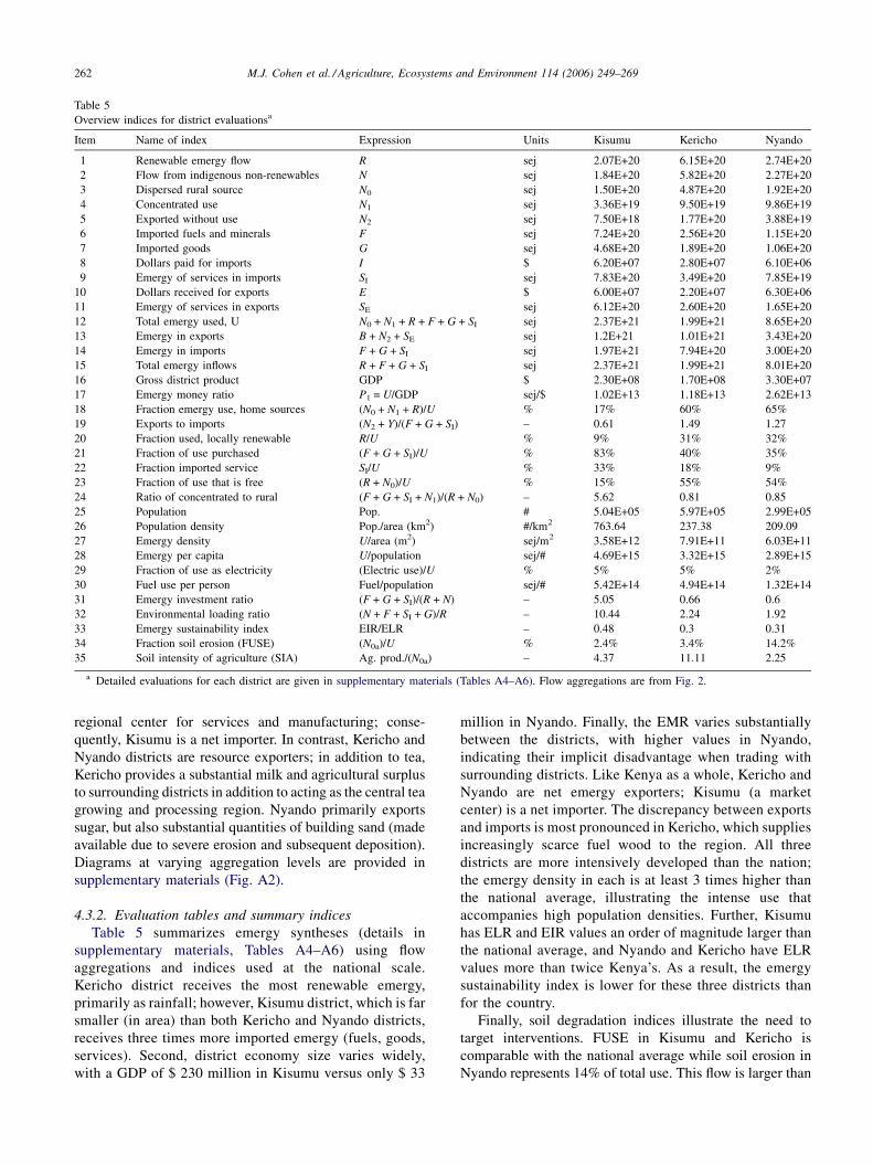
M.J. Cohen et al. / Agriculture, Ecosystems and Environment 114 (2006) 249–269262

Table 5

Overview indices for district evaluationsa

Item Name of index Expression Units Kisumu Kericho Nyando

1 Renewable emergy flow R sej 2.07E+20 6.15E+20 2.74E+20

2 Flow from indigenous non-renewables N sej 1.84E+20 5.82E+20 2.27E+20

3 Dispersed rural source N0 sej 1.50E+20 4.87E+20 1.92E+20

4 Concentrated use N1 sej 3.36E+19 9.50E+19 9.86E+19

5 Exported without use N2 sej 7.50E+18 1.77E+20 3.88E+19

6 Imported fuels and minerals F sej 7.24E+20 2.56E+20 1.15E+20

7 Imported goods G sej 4.68E+20 1.89E+20 1.06E+20

8 Dollars paid for imports I $ 6.20E+07 2.80E+07 6.10E+06

9 Emergy of services in imports SI sej 7.83E+20 3.49E+20 7.85E+19

10 Dollars received for exports E $ 6.00E+07 2.20E+07 6.30E+06

11 Emergy of services in exports SE sej 6.12E+20 2.60E+20 1.65E+20

12 Total emergy used, U N0 + N1 + R + F + G + SI sej 2.37E+21 1.99E+21 8.65E+20

13 Emergy in exports B + N2 + SE sej 1.2E+21 1.01E+21 3.43E+20

14 Emergy in imports F + G + SI sej 1.97E+21 7.94E+20 3.00E+20

15 Total emergy inflows R + F + G + SI sej 2.37E+21 1.99E+21 8.01E+20

16 Gross district product GDP $ 2.30E+08 1.70E+08 3.30E+07

17 Emergy money ratio P1 = U/GDP sej/$ 1.02E+13 1.18E+13 2.62E+13

18 Fraction emergy use, home sources (N0 + N1 + R)/U % 17% 60% 65%

19 Exports to imports (N2 + Y)/(F + G + SI) – 0.61 1.49 1.27

20 Fraction used, locally renewable R/U % 9% 31% 32%

21 Fraction of use purchased (F + G + SI)/U % 83% 40% 35%

22 Fraction imported service SI/U % 33% 18% 9%

23 Fraction of use that is free (R + N0)/U % 15% 55% 54%

24 Ratio of concentrated to rural (F + G + SI + N1)/(R + N0) – 5.62 0.81 0.85

25 Population Pop. # 5.04E+05 5.97E+05 2.99E+05

26 Population density Pop./area (km2) #/km2 763.64 237.38 209.09

27 Emergy density U/area (m2) sej/m2 3.58E+12 7.91E+11 6.03E+11

28 Emergy per capita U/population sej/# 4.69E+15 3.32E+15 2.89E+15

29 Fraction of use as electricity (Electric use)/U % 5% 5% 2%

30 Fuel use per person Fuel/population sej/# 5.42E+14 4.94E+14 1.32E+14

31 Emergy investment ratio (F + G + SI)/(R + N) – 5.05 0.66 0.6

32 Environmental loading ratio (N + F + SI + G)/R – 10.44 2.24 1.92

33 Emergy sustainability index EIR/ELR – 0.48 0.3 0.31

34 Fraction soil erosion (FUSE) (N0a)/U % 2.4% 3.4% 14.2%

35 Soil intensity of agriculture (SIA) Ag. prod./(N0a) – 4.37 11.11 2.25

a Detailed evaluations for each district are given in supplementary materials (Tables A4–A6). Flow aggregations are from Fig. 2.

regional center for services and manufacturing; conse-

quently, Kisumu is a net importer. In contrast, Kericho and

Nyando districts are resource exporters; in addition to tea,

Kericho provides a substantial milk and agricultural surplus

to surrounding districts in addition to acting as the central tea

growing and processing region. Nyando primarily exports

sugar, but also substantial quantities of building sand (made

available due to severe erosion and subsequent deposition).

Diagrams at varying aggregation levels are provided in

supplementary materials (Fig. A2).

4.3.2. Evaluation tables and summary indices

Table 5 summarizes emergy syntheses (details in

supplementary materials, Tables A4–A6) using flow

aggregations and indices used at the national scale.

Kericho district receives the most renewable emergy,

primarily as rainfall; however, Kisumu district, which is far

smaller (in area) than both Kericho and Nyando districts,

receives three times more imported emergy (fuels, goods,

services). Second, district economy size varies widely,

with a GDP of $ 230 million in Kisumu versus only $ 33

million in Nyando. Finally, the EMR varies substantially

between the districts, with higher values in Nyando,

indicating their implicit disadvantage when trading with

surrounding districts. Like Kenya as a whole, Kericho and

Nyando are net emergy exporters; Kisumu (a market

center) is a net importer. The discrepancy between exports

and imports is most pronounced in Kericho, which supplies

increasingly scarce fuel wood to the region. All three

districts are more intensively developed than the nation;

the emergy density in each is at least 3 times higher than

the national average, illustrating the intense use that

accompanies high population densities. Further, Kisumu

has ELR and EIR values an order of magnitude larger than

the national average, and Nyando and Kericho have ELR

values more than twice Kenya’s. As a result, the emergy

sustainability index is lower for these three districts than

for the country.

Finally, soil degradation indices illustrate the need to

target interventions. FUSE in Kisumu and Kericho is

comparable with the national average while soil erosion in

Nyando represents 14% of total use. This flow is larger than

M.J. Cohen et al. / Agriculture, Ecosystems and Environment 114 (2006) 249–269 263

Fig. 5. Generic land use subsystem diagram with aggregated flows (renewable—R, non-renewable—N, purchased—F, and labor/service—S), and yield (Y).

all district crop production and equivalent to 50% of imports.

SIA indicates a similar condition; agricultural activity in

Nyando has a net benefit of 2.25, substantially below the

national average. In contrast, agriculture in Kericho has a

higher SIA than the national average. The moderate SIA in

Kisumu is due to the proportion of that district that is

urbanized, leading to erosion rates not due exclusively to

agricultural activity.

4.4. Regional land use subsystem analysis

4.4.1. Subsystem descriptions

A generic diagram (Fig. 5) depicts aggregated flows and

exogenous resources derived from synthesis of management

practices, inputs and yields for each land use subsystem.

Land use yield is depicted as the interaction of renewable

resources, purchased inputs and human labor. Soil erosion is

an unintended consequence, depleting a stock of soil

functional capacity; this flow is highly variable across land

use systems. Yields generate variable cash income, which

may be used to purchase farm inputs or diverted to other

livelihood needs. More specific systems diagrams for each

subsystem are provided in supplementary materials (Figs.

A3 and A4).

Subsistence agriculture is the primary livelihood activity.

Major crops include maize, sorghum, beans, cassava, millet

and cooking bananas. For this work, we present an analysis

of maize production in both lowland and highland climate

regimes. Emergy evaluations for other crops (maize/bean

intercropping, sorghum, etc.) are presented as supplemen-

tary materials (Table A2). Maize farming in the region

makes limited use of agrochemicals (fertilizers, herbicides),

resulting in heavy reliance on human labor; improved

varieties are only occasionally used. The main renewable

input is rainfall (Jaetzold and Schmidt, 1982). Human labor

(weeding, planting, tillage, and harvesting) is an estimated

130 person-days per hectare per year.

Commercial agriculture is dominated by outgrower

operations (i.e., small farms selling yields to central

processing facilities), as opposed to large commercial

farms. An important input for both sugar and tea production

is the purchase of improved varieties (cuttings or seedlings).

Chemical inputs, primarily fertilizers, are more widely used

for commercial crops because of increased access to cash

resources from their sale. For this study, only lowland

sugarcane production was evaluated (though highland

systems exist); only highland tea growing operations were

analyzed (lowlands are outside the viable agro-climatic zone

for tea production).

Livestock production is a critical livelihood strategy

throughout rural Kenya. As population growth has forced

intensification, highland production has shifted from free

range to paddock grazing with primarily improved breeds

that are fed on pasture grasses and harvested napier grass

(Pennisetum purpureum), and require greater disease control

efforts. In contrast, communal grazing continues to be the

M.J.

Co

hen

eta

l./Ag

ricultu

re,E

cosystem

sa

nd

Enviro

nm

ent

11

4(2

00

6)

24

9–

26

92

64

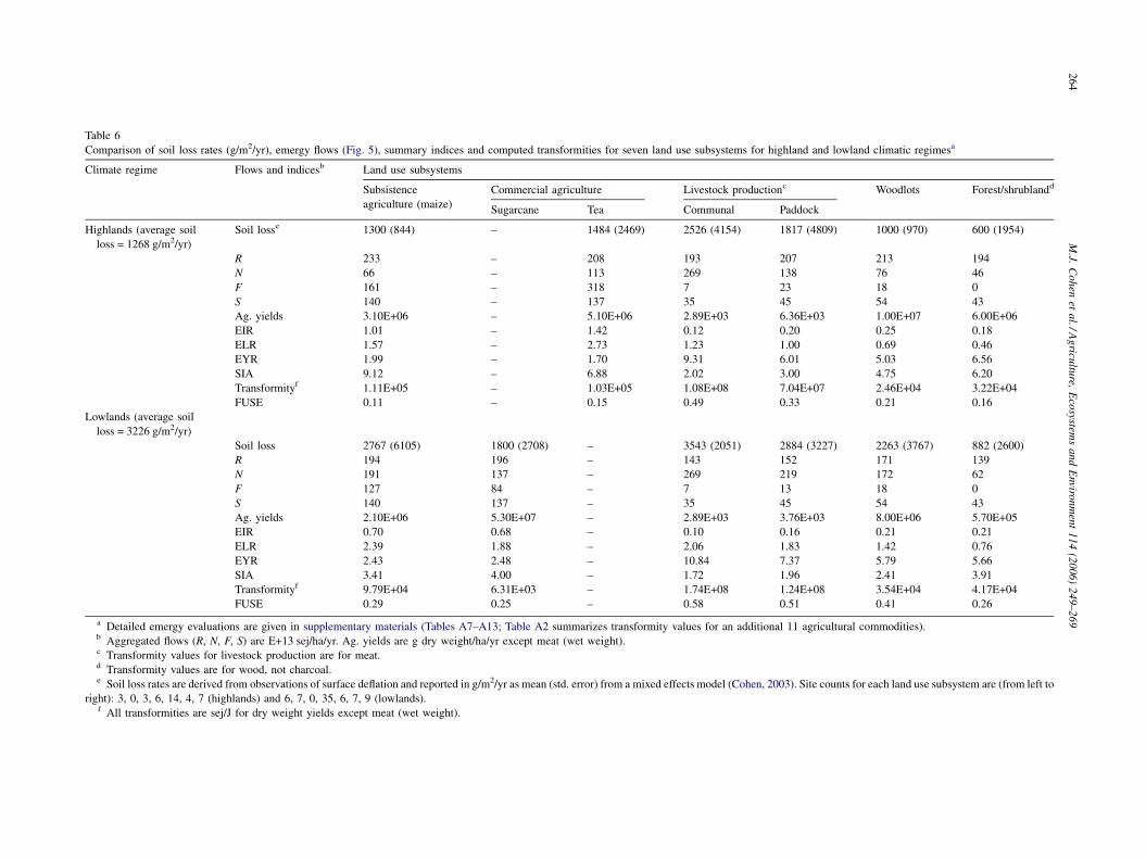
Table 6

Comparison of soil loss rates (g/m2/yr), emergy flows (Fig. 5), summary indices and computed transformities for seven land use subsystems for highland and lowland climatic regimesa

Climate regime Flows and indicesb Land use subsystems

Subsistence

agriculture (maize)

Commercial agriculture Livestock productionc Woodlots Forest/shrublandd

Sugarcane Tea Communal Paddock

Highlands (average soil

loss = 1268 g/m2/yr)

Soil losse 1300 (844) – 1484 (2469) 2526 (4154) 1817 (4809) 1000 (970) 600 (1954)

R 233 – 208 193 207 213 194

N 66 – 113 269 138 76 46

F 161 – 318 7 23 18 0

S 140 – 137 35 45 54 43

Ag. yields 3.10E+06 – 5.10E+06 2.89E+03 6.36E+03 1.00E+07 6.00E+06

EIR 1.01 – 1.42 0.12 0.20 0.25 0.18

ELR 1.57 – 2.73 1.23 1.00 0.69 0.46

EYR 1.99 – 1.70 9.31 6.01 5.03 6.56

SIA 9.12 – 6.88 2.02 3.00 4.75 6.20

Transformityf 1.11E+05 – 1.03E+05 1.08E+08 7.04E+07 2.46E+04 3.22E+04

FUSE 0.11 – 0.15 0.49 0.33 0.21 0.16

Lowlands (average soil

loss = 3226 g/m2/yr)

Soil loss 2767 (6105) 1800 (2708) – 3543 (2051) 2884 (3227) 2263 (3767) 882 (2600)

R 194 196 – 143 152 171 139

N 191 137 – 269 219 172 62

F 127 84 – 7 13 18 0

S 140 137 – 35 45 54 43

Ag. yields 2.10E+06 5.30E+07 – 2.89E+03 3.76E+03 8.00E+06 5.70E+05

EIR 0.70 0.68 – 0.10 0.16 0.21 0.21

ELR 2.39 1.88 – 2.06 1.83 1.42 0.76

EYR 2.43 2.48 – 10.84 7.37 5.79 5.66

SIA 3.41 4.00 – 1.72 1.96 2.41 3.91

Transformityf 9.79E+04 6.31E+03 – 1.74E+08 1.24E+08 3.54E+04 4.17E+04

FUSE 0.29 0.25 – 0.58 0.51 0.41 0.26

a Detailed emergy evaluations are given in supplementary materials (Tables A7–A13; Table A2 summarizes transformity values for an additional 11 agricultural commodities).b Aggregated flows (R, N, F, S) are E+13 sej/ha/yr. Ag. yields are g dry weight/ha/yr except meat (wet weight).c Transformity values for livestock production are for meat.d Transformity values are for wood, not charcoal.e Soil loss rates are derived from observations of surface deflation and reported in g/m2/yr as mean (std. error) from a mixed effects model (Cohen, 2003). Site counts for each land use subsystem are (from left to

right): 3, 0, 3, 6, 14, 4, 7 (highlands) and 6, 7, 0, 35, 6, 7, 9 (lowlands).f All transformities are sej/J for dry weight yields except meat (wet weight).

M.J. Cohen et al. / Agriculture, Ecosystems and Environment 114 (2006) 249–269 265

primary strategy in the lowlands despite relatively high stock

densities. Cattle are primarily Zebu breed, which tend to be

resistant to diseases typical in ruminants in tropical Africa

(Simpson and Evangelou, 1984), and preferred where access

to veterinary services are limited. Labor requirements for

paddock grazing are higher, but are offset by substantially

higher milk and meat yields than for lowland animal

husbandry.

Supplies of fuelwood and timber are limited, making

managed forests critical in both zones. Lowland woodlots

are comprised of species adapted to �1000 mm of annual

rainfall (e.g., Acacia spp., Terminalia brownii, Grevillea

robusta). Highland systems are dominated by Eucalyptus

spp. and Acacia mearnsii, in addition to other species that

coppice readily. A common practice in the highlands is

harvesting tree leaves as fodder for paddock-grazed animals.

Labor requirements are relatively high during initial

planting, but reduce substantially until harvest; coppicing

reduces subsequent labor investment. Turnover times for

maximal woodlot yield are between 8 and 12 years; one

hectare produces roughly 100 m3 of wood over that period.

Native forest cover (both highland broadleaf forests and

lowland shrublands) has been reduced to remnant patches,

primarily on steep escarpment slopes with low population

densities. Charcoal production is a major yield from these

communal lands despite 85% energy loss during conversion

(Chavangi and Zimmermann, 1987). Frequently, soils

beneath these wooded systems are shallow and stony

because of their location on steep escarpments, so limited

use is made of the land after clearing. Labor is directed at

harvesting and charcoal-firing; profits are not reinvested

(e.g. replanting, soil stabilization) (Chavangi and Zimmer-

mann, 1987).

4.4.2. Soil loss rates

Observed erosion rates by land use and climate zone

(Table 6) correspond reasonably with national published

rates for Kenya (Table 1). Disparities include significantly

higher observed rates in forests/shrublands, dramatically

different rates between highland and lowland subsistence

agriculture and significant variability within land use

categories. For lowland and highland animal husbandry,

soil loss rates were high (range 1817–3543 g/m2/yr),

particularly for communal grazing sites. Woodlots in the

highlands were relatively protective, but lowland woodlots

exhibited rapid loss rates (1000 versus 2263 g/m2/yr,

respectively), primarily as a result of limited ground-cover.

The lowest soil loss on managed lands in the lowlands was

for small-scale sugarcane production (1800 g/m2/yr); loss

rates under highland commercial tea production were

similar (1484 g/m2/yr). Additional observations were made

in wetlands (limited erosion pin retrieval due to deposition)

and severely degraded lands (max loss = 25,000 g/m2/yr;

mean = 13,500 g/m2/yr). Overall, rates were three times

higher in the lowlands (Vertisols/Planosols, sodic phases,

frequent drought) than in the highlands (Nitosols). Using

baseline weathering rates as a benchmark (�100 g/m2/yr for

tropical conditions; Pimentel, 1993), these values are clearly

unsustainable, even for less exploited systems (e.g., shrub-

lands supporting low density grazing).

4.4.3. Emergy analyses

Emergy syntheses for each subsystem are summarized in

Table 6 (details in supplementary materials)—aggregate

flows are from Fig. 2. All indices (including soil loss rates)

can be directly compared across land uses and climatic zones

except transformity, which is specific to each subsystem’s

product (transformity comparison across climate regimes is

informative). Comparing SIA between systems (at this scale,

SIA = 1/FUSE), we observe that subsistence agriculture

followed by commercial tea production and forest charcoal

operations (9.12, 6.88 and 6.20, respectively) provide the

highest net benefit in the highland climatic zone. Both forms

of animal husbandry have substantially lower SIA values

than other land uses. For lowland subsystems, the highest

SIA is for sugarcane production, followed by charcoal

production, and subsistence agriculture (4.0, 3.91 and 3.41,

respectively). As before, livestock land uses are lower, with

erosion representing over 60% of use for lowland communal

grazing.

The EIR, ELR and EYR offer additional information

about the ability of each land use to integrate in the larger

economic system. For example, EIR for highland tea

production indicates strong attraction potential for external

resources while wood production systems appear to give

high yield (EYR > 6) but attract little outside investment.

ELR values are higher in the lowlands as a result of elevated

erosion rates in that zone. High EYR for communal

livestock production in the lowlands illustrates the need for

indices like SIA and FUSE, because most of the yield in that

system is lost soil. As a result, the transformity of meat is an

order of magnitude larger than transformities for other

production systems that have been evaluated (Brandt-

Williams, 2001).

5. Discussion

Our primary objective – to place the estimated ecosystem

value of soil in a national economic context – can be

demonstrated by computing the equivalent economic

product due to a soil stock. Dividing the emergy content

of one hectare of topsoil organic carbon by the national

EMR (1.17E13 sej/$), this equates to US$ 11,000 per

hectare. The transformity of SOM in this work is nearly

twice as high as previous calculations (1.07E+05 sej/J for

temperate forest soils; Odum, 1996). The observed

difference is a result of different organic matter accretion

dynamics in the tropics where sub-humid conditions, warm

temperatures, and termites result in rapid oxidation rates

that are manifest in the small quantity of recalcitrant soil

organic carbon entering the SOM pool each year. Since

M.J. Cohen et al. / Agriculture, Ecosystems and Environment 114 (2006) 249–269266

Table 7

Comparison of Kenyan summary indices with other national economies (nations are sorted by the national fraction soil erosion (FUSE))

Year U U:P U:A GDP EMR ELR FUSE (%) SIA

Kuwaita 1996 5.74E+22 3.39E+16 3.22E+12 3.10E+10 1.85E+12 6.24 0.01 –a

Canadaa 2001 2.68E+24 8.78E+16 2.91E+11 5.99E+11 4.47E+12 3.07 0.02 49.5

Japana 2001 3.59E+24 2.83E+16 9.51E+12 4.50E+12 7.98E+11 2.88 0.02 37.8

Switzerlanda 2000 2.54E+23 3.52E+16 6.15E+12 2.70E+11 9.40E+11 2.85 0.12 64.4

Botswanaa 1996 3.99E+22 2.85E+15 6.86E+10 4.00E+09 9.97E+12 0.28 0.13 27.9

Francea 2001 1.32E+24 2.21E+16 2.39E+12 1.40E+12 9.43E+11 26.06 0.27 42.1

USAb 1999 1.18E+25 4.18E+16 1.25E+12 9.94E+12 1.19E+12 8.1 0.44 81.9

Australiaa 2001 1.63E+24 8.41E+16 2.13E+11 3.40E+11 4.80E+12 0.3 0.61 25.6

Irelanda 1996 4.67E+22 3.33E+15 6.64E+11 5.90E+10 2.68E+12 3.32 0.76 70.9

Brazilc 1994 3.10E+24 2.20E+16 3.63E+11 7.20E+11 4.32E+12 0.75 1.77 15.6

Chinaa 2001 6.64E+24 5.17E+15 7.12E+11 9.80E+11 6.78E+12 1.23 2.15 22.5

Indiaa 2001 2.62E+24 9.31E+15 7.96E+11 4.42E+11 5.93E+12 33.05 2.91 11.1

Tanzaniaa 1998 4.78E+22 2.01E+15 4.62E+10 3.07E+09 1.56E+13 0.14 3.32 11.4

Kenyad 2001 1.20E+23 3.77E+15 2.07E+11 1.02E+10 1.17E+13 0.80 3.77 7.6

Malawia 1996 7.67E+21 9.35E+14 6.45E+10 1.50E+09 5.12E+12 0.4 4.12 3.1

South Africaa 2001 9.26E+23 2.14E+16 7.72E+11 4.12E+11 2.25E+12 1.3 4.35 9.6

Guatemalaa 1996 1.28E+22 7.63E+15 8.10E+11 3.67E+10 2.40E+12 0.49 4.75 11.3

Sources: (a) M.T. Brown (unpublished data), (b) G. Stachetti (unpublished data), (c) Odum (1996), (d) this study. All values in this table are reported for the

Odum (2000) common emergy benchmark.a Kuwaiti agriculture is extremely limited; the computed SIAvalue is inappropriate. U: total emergy use, P: population, A: area, GDP: gross national product,

EMR: emergy money ratio, ELR: environmental loading ratio, ESI: emergy sustainability index, FUSE: fraction soil erosion, SIA: soil intensity of agriculture.

transformity measures environmental work embodied in a

product, doubling the transformity indicates a doubling of

ecosystem value. Additional refinements (developing a

transformity value for particular soil types) are clearly

needed.

Transformity values for other commodities were,

surprisingly, not substantially different between temperate

and tropical productions systems. For example, the

transformity for maize in Kenya was computed as

1.11E5 sej/J; by comparison, corn in Florida has a

transformity of 1.26E5 sej/J (Brandt-Williams, 2001).

However, we view the use of locally computed transformity

values for analysis as a major priority for refinements to the

emergy methodology.

Among the significant findings at the national scale are

levels of summary indices (trade balance, sustainability) and

the magnitude of soil erosion. Table 7 summarizes some

indices in comparison with other nations. Kenya clearly has

low emergy per capita (falling in 4th quartile) and high EMR.

A moderate trade imbalance (E:I = 1.23), typical of devel-

oping nations (Odum, 1996; Brown, 2003), occurs because

the Kenyan EMR (1.17E13 sej/$) is an order of magnitude

higher than the world EMR (2.08E12 sej/$) suggesting that

each unit of standardized currency ($) has greater purchasing

power in Kenya than in global markets. ELR for Kenya is

relatively high, particularly given the small economic product

(GDP) generated by that environmental load.

Of particular interest is the magnitude of soil erosion

(4.52E21 sej/yr) in comparison with other national flows

(Table 3); soil loss is comparable to total national electricity

production or agricultural exports, and only slightly smaller

than the national tourist industry. When put in equivalent

dollar units, soil loss represents a cost to Kenya of $ 390

million; forest losses add an additional $ 350 million for a

total annual natural capital depletion equivalent to over 7%

of GDP.

Comparison of FUSE and SIA with other nations

(Table 7) reveals that, while FUSE is higher in Malawi,

Guatemala, and South Africa, only Malawi has the

combined condition of high FUSE and low SIA as was

observed in Kenya. This demonstrates the compounding

effects of low input agriculture and high-risk soils/land uses

on national soil conservation needs in sub-Saharan Africa.

The advantage of using these indices as a benchmark for

national or regional analysis (particularly through time) is

that they relate both erosion and production, embodying the

tradeoffs between increased land use intensity and the

external costs thereof.

At the district scale, local targeting of intervention

resources is needed. While total flows (sej/yr) are not

comparable between nation and district (or between districts

of different size), scaled flows (per capita and per area) and

all ratio indices (ELR, EIR, FUSE, SIA, etc.), are

comparable. The national EMR (1.17E13) is larger than

the EMR for Kisumu and Kericho, and nearly half that of

Nyando suggesting that the former two benefit from within-

country trade, while the latter is at an implicit disadvantage.

As with trade between nations with differing EMR, this

arises because each unit of currency flowing into Nyando

buys more real wealth than can be purchased from outside.

The % electricity, FUSE, SIA and emergy per capita all

reinforce the qualitative observation of acute poverty and

environmental degradation in Nyando.

Our observations of approximate soil erosion rates across

the landscape demonstrate dramatic variability observed

within what are treated as homogeneous units (e.g., lowland

M.J. Cohen et al. / Agriculture, Ecosystems and Environment 114 (2006) 249–269 267

annual cropping systems, highland woodlots; Table 6). Their

approximate consistency with other published values

suggest that they the method is reliable, and our resulting

ability discriminate between erosion rates across land-use

subsystems and climate zone make them useful for this

work. The main assumption that differs between scales – that

of the sediment yield ratio – necessitates further refinements

to the way that erosion losses are evaluated.

At the land use subsystem scale, pronounced differences in

the system-scale costs and benefits between different land

uses are observed. As an example, compare indices and

transformity values across climatic zones. Despite higher

renewable inputs in the highlands, transformity values are

generally lower than in the lowlands, suggesting comparative

ecological advantage of highland agriculture. The largest

differences are for subsistence agriculture and woodlot

production. When comparing like products, systems that

produce a product with the lowest level of input (i.e.,

maximize system scale efficiency by minimizing transfor-

mity) should be reinforced through policy. Those land uses

exhibiting lower efficiencies should be converted to other uses

that maximize local comparative advantage (e.g., conversion

of communal livestock systems to sugarcane for lowland

areas) to enhance overall system performance.

The SIA index can be used to orient policy on selecting

appropriate land use subsystems. While erosion rates in the

lowlands are comparable between subsistence maize crop-

ping and paddock grazing, the SIA is substantially different

(3.41 versus 1.96, respectively). Similarly, while the loss rates

under sugarcane production are more than double those under

shrublands, the SIA would suggest that this is a reasonable

trade-off with respect to overall benefit. Finally, while

woodlots may tend to reduce erosion rates in the highlands vis

a vis agricultural systems, the net benefit of that protection

does not outweigh the benefits of increased productivity.

Constraints to reorienting the regional system given

prevailing poverty among the rural subsistence farmers are

clear; in particular, the socio-cultural importance of animal

husbandry and reliance on subsistence production are

impediments to regional optimization, and efforts to

improve land management at the large scale will need to

simultaneously address food/fuel security issues. Difficult as

it is to imagine or affect large-scale transformation of

landscapes and livelihoods in the region, findings such as

these need to be incorporated in regional planning.

We view linkages between scales as a crucial outcome of

our work. While the scope and intensity of the problem at the

national scale warrants capital investments from government,

where and how to maximize investment effectiveness requires

nested analyses. The ability of government to provide

incentives or discourage land use practices as necessary

requires resources be made available and an understanding of

how to use them emerges. Assessing the national condition

with respect to natural capital depletion provides essential

context for interpreting analyses at smaller scales, and

analyses at smaller scales offer preliminary insight on how

resources mobilized at the large scale are best employed.

Further, comparative analysis between land uses, districts and

other nations places findings in perspective, and could aid

non-governmental organizations in prioritizing their inter-

vention, research and educational activities.

6. Conclusions

1. Soil erosion represents a significant hidden cost of

development at multiple scales in Kenya’s environmen-

tal/economic system. At the national scale, 3.8% of total

emergy use is due to soil loss (an additional 3.5% is due

to forest clearing), equivalent to $ 390 million in macro-

economic value or to the value of agricultural exports or

electricity production.

2. A

nalysis of three districts in western Kenya showed that

erosion is particularly serious in Nyando district, which,

in contrast to Kisumu (manufacturing) and Kericho

(commercial tea production) districts, has limited

economic infrastructure. Soil erosion represents almost

15% of total use in Nyando; lowland agriculture

practiced there has a net benefit of 2.25:1, which

indicates deeply marginalized rural farmers.

3. L

and subsystems reveal dramatic differences in their

emergy basis, both between land use and climatic zone.

Animal husbandry operations, and particularly commu-

nal grazing, have low SIA values; for lowland communal

grazing, 60% of total emergy use is erosion.

4. P

lant-based subsistence and commercial agricultural

activities are more sustainable with respect to soil loss

and net agricultural benefit than other land uses (e.g.,

communal livestock production). Woodlot operations are

effective land uses in the highlands, but demonstrate

limited potential in the lowlands, where soil loss rates

under planted forests were high.

5. O

verall, there is a need to translate the quantitative

findings of this work into three policy outcomes. First,

improved resource allocation towards attenuating soil

loss are clearly necessary based on the apparent problem

magnitude. Second, resources need to be targeted for

maximum effect, whereby districts and regions that are

particularly at-risk should receive the bulk of any external

assistance. Finally, incentives to encourage appropriate

land use planning with respect to maximizing net benefit

of rural agriculture need to be devised.

Appendix A. Supplementary data

Supplementary data associated with this article can be

found, in the online version, at 10.1016/j.agee.2005.10.021.

References

Alejandro Prado-Jatar, M., Brown, M.T., 1997. Interface ecosystems with an

oil spill in a Venezuelan tropical savannah. Ecol. Eng. 8, 49–78.

M.J. Cohen et al. / Agriculture, Ecosystems and Environment 114 (2006) 249–269268

Alfsen, K.H., DeFranco, M.A., Glomsrod, S., Johnson, T., 1996. The cost of

soil erosion in Nicaragua. Ecol. Econ. 16, 129–145.

Alin, S.R., O’Reily, C.M., Cohen, A.S., Dettman, D.L., Palacios-Fest, M.R.,

McKee, B.A., 2002. Effects of land-use change on aquatic biodiversity:

a view from the paleorecord at Lake Tanganyika, East Africa. Geology

30, 1143–1146.

Bandara, J.S., Chisholm, A., Ekanayake, A., Jayasuriya, S., 2001. Environ-

mental costs of soil erosion in Sri Lanka: tax/subsidy policy options.

Environ. Model. Software 16, 497–508.

Barber, R.G., 1983. Magnitudes and sources of soil erosion in some humid

and semi-arid parts of Kenya and the significance of soil loss tolerance

values in soil conservation in Kenya. Soil and water conservation in

Kenya. In: Proceedings of the Second National Workshop, Institute for

Development Studies, University of Nairobi, Kenya.

Bojo, J., 1996. The costs of land degradation in sub-Saharan Africa. Ecol.

Econ. 16, 161–173.

Brandt-Willams, S. 1999. Evaluation of watershed control of two Central

Florida lakes: Newnans Lake and Lake Weir. Ph.D. Dissertation.

University of Florida, Gainesville, FL.

Brandt-Williams, S., 2001. Handbook of Emergy Evaluation: Folio #4—

Emergy of Florida Agriculture. Center for Environmental Policy, Uni-

versity of Florida, Gainesville, FL.

Brooks, K.N., Ffolliot, P.F., Gregerson, H.M., DeBano, L.F., 1997. Hydrol-

ogy and the Management of Watersheds, 2nd ed. Iowa State University

Press, Ames, IA.

Brown, M.T., 2003. Resource imperialism: emergy perspectives on sustain-

ability, balancing the welfare of nations and international trade. In:

Ulgiati, S. (Ed.), Proceedings of the Conference on Advances in Energy

Studies Held in Porto Venere, Italy. October. University of Siena, Italy.

Brown, M.T., Buranakarn, V., 2003. Emergy indices and ratios for sustain-

able material cycles and recycle options. Resour. Conserv. Recycl. 38,

1–22.

Brown, M.T., McClanahan, T.R., 1996. Emergy analysis perspectives of

Thailand and Mekong River Dam proposals. Ecol. Model. 91, 105–130.

Brown, M.T., Ulgiati, S.M., 1999. Emergy evaluation of the biosphere and

natural capital. Ambio 28, 486–493.

Buenfil, A., 2001. Emergy analysis of water. Ph.D. Dissertation. University

of Florida, Gainesville, FL.

Chavangi, A.H., Zimmermann, R., 1987. A Guide to Farm Forestry in

Kenya. Ministry of Environment and Natural Resources, Nairobi,

Kenya.

Chipeta, G.B., 1976. A study of wind power availability in Kenya. Ph.D.

Dissertation. University of Nairobi, Kenya.

Christensen, V., 1994. Emergy-based ascendancy. Ecol. Model. 72, 129–

144.

Clark, E.H., 1987. Soil erosion: offsite environmental effects. In: Harlin,

J.M., Bernardi, G.M. (Eds.), Soil Loss: Processes, Policies, and Pro-

spects. Westview, New York, pp. 59–89.

Cleveland, C.J., Costanza, R., Hall, C.A.S., Kauffman, R., 1984. Energy and

the United States economy: a biophysical perspective. Science 225,

890–897.

Cohen, M.J., 2003. Systems evaluation of erosion and erosion control in a

tropical watersheds. Ph.D. Dissertation. University of Florida, Gaines-

ville, FL.

Cohen, M.J., Shepherd, K.D., Walsh, M.G., 2005. Empirical reformulation

of the universal soil loss equation for erosion risk assessment in a

tropical watershed. Geoderma 124, 235–252.

Coleman, D.C., Oades, J.M., Uehara, G., 1989. Dynamics of Soil Organic

Matter in Tropical Ecosystems. University of Hawaii Press, Honolulu,

HI.

Corbett, J.D., Collis, S.N., Bush, B.R., Muchugu, E.I., Jeske, R.Q., Burton,

R.A., Martinez, R.E., White, J.W., Hodson, D.P., 1997. Almanac

Characterization Tool—Geospatial Database. Blacklands Research

Center, Texas Agricultural Experiment Station, Texas A&M University,

College Park, TX, USA.

Crosson, P.R., 1986. Soil erosion and policy issues. In: Phipps, T.T.,

Crosson, P.R., Price, K.A. (Eds.), Agriculture and the Environment.

National Center for Food and Agricultural Policy, Resources for the

Future, Washington, DC, USA.

Crosson, P.R., 1995. Soil erosion estimates and costs. Science 269, 461–

464.

Crul, R.C., 1995. Limnology and Hydrology of Lake Victoria. UNESCO

Publishing, Dijon, France.

Doherty, S.J., Nilsson, P.O., Odum, H.T., 2002. Emergy Evaluation of Forest

Production and Industries in Sweden. Institutionen for Bioenergi,

Uppsala, Sweden.

Duxbury, J.M., 1995. The significance of greenhouse gas emissions from

soils tropical agroecosystems. In: Lal, R., Kimble, J., Levine, E., Ste-

wart, B.A. (Eds.), Soil Management and Greenhouse Effect. CRC Press,

Boca Raton, FL, pp. 279–292.

Eggermont, H., Verschuren, D., 2003. Impact of soil erosion in disturbed

tributary drainages on the benthic invertebrate fauna of Laka Tanga-

nyika, East Africa. Biol. Conserv. 113, 99–109.

Enters, T., 1997. In: Agus, F.W.T.F., Kerr Penning de Vries, J. (Eds.), A

Framework for the Economic Assessment of Soil Erosion and Soil

Conservation. Soil Erosion at Multiple Scales: Principles and Methods

for Assessing Causes and Impacts. CABI Publishing, Wallingford, UK.

Europa Publications, 2000. Europa World Year Book 1999, vol. II. Europa

Publications.

Food and Agricultural Organization and United Nations (FAO-UN), 1999.

FAO Trade and Commerce Yearbook 1998. United Nations, Rome.

Food and Agricultural Organization (FAO), 2001. Atlas of Water Resources

and Irrigation in Africa, FAO Land and Water Digital Media Series #13.

FAO, Rome, Italy.

Gachene, C.K., Jarvis, K.N.J., Linner, H., Mbuvi, J.P., 1997. Soil erosion

effects on soil properties in a highland area of Central Kenya. Soil Sci.

Soc. Am. J. 61, 559–564.

Hall, C.J., Lindenberger, D., Kuemmel, R., Kroeger, T., Eichhorn, W., 2001.

The need to reintegrate the natural sciences with economics. Bioscience

51, 663–673.

Harvey, C.A., Pimentel, D., 1996. Effects of soil and wood depletion on

biodiversity. Biodiv. Conserv. 5, 1121–1130.

Howington, T.M., 1999. A spatial analysis of emergy of an internationally

shared drainage basin and the implications for policy decisions. Ph.D.

Dissertation. University of Florida, Gainesville, FL.

ICRAF, 2000. Improved Land Management in the Lake Victoria Basin—

First Report of Progress and Results July 1999 to March 2000. ICRAF

Working Paper, Nairobi, Kenya.

Jaetzold, R., Schmidt, H., 1982. Farm Management Handbook of Kenya—

Natural Conditions and Farm Management Information, vol. II (West

Kenya) Ministry of Agriculture, Kenya, Rossdorf, Germany.

Kaufman, L., Chapman, L.J., Chapman, C.A., 1996. The Great Lakes. In:

McClanahan, T.R., Young, T.P. (Eds.), East African Ecosystems and

their Conservation. Oxford University Press, New York, NY.

Kelley, D.W., Nater, E.A., 2000. Historical sediment flux from three

watersheds into Lake Pepin, Minnesota, USA. J. Environ. Qual. 29,

561–568.

Kenya Central Bureau of Statistics, 2000. Statistical Abstract: Republic of

Kenya. Ministry of Finance and Planning, Nairobi, Kenya.

Kerr, J., 1997. In: Agus, F.W.T.F., Kerr Penning de Vries, J. (Eds.), The

Economics of Soil Degradation: From National Policy to Farmers’

Needs. Soil Erosion at Multiple Scales: Principles and Methods for

Assessing Causes and Impacts. CABI Publishing, Wallingford, UK.

Kiome, R.M., Stocking, M., 1995. Rationality of farmer perception of soil

erosion: the effectiveness of soil conservation in semi-arid Kenya. Glob.

Environ. Change 5 (4), 281–295.

Lagerberg, C., 1999. Emergy analysis of the resource use in greenhouse

crop production and of the resource basis of the Swedish economy.

Ph.D. Dissertation. Swedish University of Agricultural Sciences,

Uppsala, Sweden.

Lal, R., 1985. Soil erosion and sediment transport research in tropical

Africa. Hydrol. Sci. J. 30, 239–256.

Lal, R., 1995. Erosion–crop productivity relationships for the soils of

Africa. Soil Sci. Soc. Am. J. 59, 661–667.

M.J. Cohen et al. / Agriculture, Ecosystems and Environment 114 (2006) 249–269 269

Lal, R., 2003. Soil erosion and the global carbon budget. Environ. Int. 29,

437–450.

Lindenschmidt, K.E., Suhr, M., Magumba, M.K., Hecky, R.E., Bugenyi,

F.W.B., 1998. Loading of solute and suspended solids from rural

catchment areas flowing into Lake Victoria. Water Resour. 32, 2776–

2786.

Loehman, E.T., Randhir, T.O., 1999. Alleviating soil erosion/pollution stock

externalities: alternative roles for government. Ecol. Econ. 30, 24–29.

Ludwig, D., 2000. Limitations of economic valuation of ecosystems.

Ecosystems 3, 31–35.

Lufafa, A., Tenywa, M.M., Isabirye, M., Majaliwa, M.J.G., Woomer, P.L.,

2002. Prediction of soil erosion in Lake Victoria basin catchment using

GIS-based universal soil loss model. Agric. Syst. 73, 1–12.

Ministry of Water Development, 1992. The Study on the National Water

Master Plan: Hydrologic Data. Japan International Cooperation Agency,

Republic of Kenya.

Morgan, R.P.C., 1995. Soil Erosion and Conservation, 2nd ed. Longman

Group Limited, Essex, UK.

Mulengera, M.K., Payton, R.W., 1999. Modification of the productivity

index model. Soil Till. Res. 52, 11–19.

Nye, P.H., Greenland, D.J., 1960. The Soil Under Shifting Cultivation.

Commonwealth Soils Technology Community, p. 51.

Ochumba, P.B.O., 1990. Massive fish kills within the Nyanza Gulf of Lake

Victoria, Kenya. Hydrobiologia 208, 93–99.

Odum, H.T., 1988. Self-organization, transformity, and information.

Science 242, 1132–1138.

Odum, H.T., 1994. Ecological and General Systems: An Introduction to

Systems Ecology, 2nd ed. University Press of Colorado, Niwot, CO.

Odum, H.T., 1996. Environmental Accounting: Energy and Environmental

Decision Making. John Wiley and Sons Inc., New York.

Odum, H.T., 2000. Folio #2: Emergy of Global Processes. Handbook of

Emergy Evaluation. Center for Environmental Policy, University of

Florida, Gainesville, FL.

Odum, H.T., Brown, M.T., Brandt-Williams, S., 2000a. Folio #1: Introduc-

tion and Global Budget. Handbook of Emergy Evaluation. Center for

Environmental Policy, University of Florida, Gainesville, FL.

Odum, H.T., Doherty, S.J., Scatena, F.N., Kharecha, P.A., 2000b. Emergy

evaluations of reforestation alternatives in Puerto Rico. Forest Sci. 46,

521–530.

Oostwoud, D.J., Bryan, R., 2001. Gully-head erosion processes and semi-

arid valley floor of Kenya: a case study into temporal variation and

sediment budgeting. Earth Surf. Process. Landforms 26, 911–933.

Parton, W., Woomer, P., Martin, A., 1994. Modeling soil organic matter

dynamics and plant productivity in tropical ecosystems. In: Woomer,

P., Swift, M. (Eds.), The Biological Management of Tropical Soils

Fertility. Wiley–Sayce, San Francisco, CA.

Pimentel, D., 1993. World Soil Erosion and Conservation. Cambridge

University Press, Cambridge, UK.

Pimentel, D., Harvey, C., Resosudarmo, P., Sinclair, K., Murz, D., McNair,

M., Crist, S., Shpritz, L., Fitton, L., Saffouri, R., Blair, R., 1995.

Environmental and economic costs of soil erosion and conservation

benefits. Science 267, 1117–1122.

Pimentel, D., Kounang, N., 1998. Ecology of soil erosion in ecosystems.

Ecosystems 1, 418–426.

Pollack, H.N., Hurter, S.J., Johnson, J.R., 1993. Heat flow from the earth’s

interior: analysis of the global data set. Rev. Geophys. 31, 267–280.

Portela, R., 1999. Energy evaluation of large scale development projects:

Mato Grosso Natural Resource Management Project, a case study. MS

Thesis. University of Florida, Gainesville, FL.

Pretty, J.N., Brett, C., Gee, D., Hine, R.E., Mason, C.F., Morison, J.I.L.,

Raven, H., Rayment, M.D., van der Bijl, G., 2000. An assessment of the

total external costs of UK agriculture. Agric. Syst. 65, 113–136.

Pritchard Jr., L., Folke, C., Gunderson, L., 2000. Valuation of ecosystem

services in institutional context. Ecosystems 3, 36–40.

Raikes, P., 1983. Livestock Development and Policy in East Africa. African

Publishing Company, New York, NY.

Romitelli, M.S., 1997. Emergy basis of watersheds. Ph.D. Dissertation.

University of Florida, Gainesville, FL.

Rural Planning Department, 1997a. Kericho District Development

Plan. Ministry of Planning and National Development, Nairobi,

Kenya.

Rural Planning Department, 1997b. Kisumu District Development Plan.

Ministry of Planning and National Development, Nairobi, Kenya.

Rural Planning Department, 1997c. Nyando District Development Plan.

Ministry of Planning and National Development, Nairobi, Kenya.

Sanchez, P.A., Shepherd, K.D., Soule, M.J., Place, F.M., Buresh, R.J., Izac,

A.N., Mokwunye, A.U., Kwesiga, F.R., Ndiritu, C.G., Woomer, P.L.,

1997. Soil fertility replenishment in Africa: an investment in natural

resource capital. In: Replenishing Soil Fertility in Africa, Soil Science

Society of America Special Publication #51, Soil Science Society of

America, Madison, WI.

Simpson, J.R., Evangelou, P., 1984. Livestock Development in Sub-Saharan

Africa: Constraints, Prospects, Policy. Westview Press, Boulder, CO.

Smaling, E., 1993. An Agro-Ecological Framework for Integrated Nutrient

Management with Special Reference to Kenya. Landbouwuniversiteit te

Wageningen, Waginingen, Netherlands.

Starett, D.A., 2000. Shadow pricing in economics. Ecosystems 3, 16–

20.

Stocking, M., 1995. Soil erosion in developing countries: where geomor-

phology fears to tread! Catena 25, 253–267.

Thomas, D.B., Senga, W.M., 1983. Soil and water conservation in Kenya.

In: Proceedings of the Second National Workshop. Institute of Devel-

opment Studies, Nairobi, Kenya.

Tiffen, M., Mortimore, M., Gichuki, F., 1994. More People Less Erosion:

Environmental Recovery in Kenya. John Wiley, Chichester, NY.

Tilley, D.R., Swank, W.T., 2003. EMERGY-based environmental systems

assessment of a multi-purpose temperate mixed-forest watershed of the

southern Appalachian Mountains, USA. J. Environ. Manage. 69, 213–

227.

Tinker, P.B., 1997. The environmental implications of intensified land use in

developing countries. Philos. Trans. Roy. Soc. Lond. B 352, 1023–1033.

Ulgiati, S.M., Brown, M.T., 1998. Monitoring patterns of sustainability of

natural and man-made ecosystems. Ecol. Model. 108, 23–36.

Ulgiati, S., Odum, H.T., Bastianoni, S., 1994. Emergy use, environmental

loading and sustainability: an emergy analysis of Italy. Ecol. Model. 73,

215–268.

United States Department of Commerce–National Oceanic and Atmo-

spheric Administration, 1994. Tide Tables 1995—Central and Western

Pacific Ocean and Indian Ocean. Tide Table—High and Low Water

Predictions NOAA.

United Nations, 2000. International Trade Statistics Yearbook 1998.

Dept. of Economic and Social Affairs, Statistics Division, New York,

NY.

Walling, D.E., 2000. Linking land use, erosion and sediment yields in river

basins. Hydrobiologia 410, 223–240.

World Bank, 1996. African Development Indicators. World Bank, Washing-

ton, DC.

World Bank, 2002. Kenya—at a glance. World Bank National summary

statistics. http://www.worldbank.org/data/countrydata/aag/ken_aag.pdf.

Young, A., 1976. Tropical Soils and Soil Survey. Cambridge University

Press, Cambridge, UK.

Zobisch, M.A., Richter, C., Heiligteig, B., Schlott, R., 1995. Nutrient losses

from cropland in the central highlands of Kenya due to surface runoff

and soil erosion. Soil Till. Res. 33, 109–116.