estimating real-time traffic carbon dioxide emissions based on intelligent transportation system...

IEEE TRANSACTIONS ON INTELLIGENT TRANSPORTATION SYSTEMS, VOL. 14, NO. 1, MARCH 2013 469

Estimating Real-Time Traffic Carbon DioxideEmissions Based on Intelligent Transportation

System TechnologiesXiaomeng Chang, Bi Yu Chen, Qingquan Li, Xiaohui Cui, Member, IEEE, Luliang Tang, and Cheng Liu

Abstract—In this paper, a bottom–up vehicle emission modelis proposed to estimate real-time CO2 emissions using intelligenttransportation system (ITS) technologies. In the proposed model,traffic data that were collected by ITS are fully utilized to estimatedetailed vehicle technology data (e.g., vehicle type) and drivingpattern data (e.g., speed, acceleration, and road slope) in theroad network. The road network is divided into a set of smallroad segments to consider the effects of heterogeneous speedswithin a road link. A real-world case study in Beijing, China, iscarried out to demonstrate the applicability of the proposed model.The spatiotemporal distributions of CO2 emissions in Beijing areanalyzed and discussed. The results of the case study indicate thatITS technologies can be a useful tool for real-time estimations ofCO2 emissions with a high spatiotemporal resolution.

Index Terms—Air pollution, carbon dioxide (CO2) emissions,intelligent transportation systems (ITSs), International VehicleEmissions (IVE) model.

NOMENCLATURE

α Index of a lane.θ Slope of a road segment.φ Index of a road segment.ϕ Traffic flow of a lane.γ Length of a lane.λ Index of a vehicle type.� Number of vehicles.ω Number of lanes within a road segment.a Vehicle acceleration (in square meters

per second).b Index of a VSP bin.esampling CO2 emission error due to the GPS sam-

pling error.f[k] Percentage of vehicles in technology

category k.

Manuscript received February 22, 2012; revised June 6, 2012; acceptedSeptember 10, 2012. Date of publication October 5, 2012; date of currentversion February 25, 2013. This work was supported in part by the NationalNatural Science Foundation of China under Grant 41071285, Grant 40830530,and Grant 41201466 and by the U.S. Department of Energy under ContractDE-AC05-00OR22725. The Associate Editor for this paper was S. Tang.

X. Chang, B. Y. Chen, Q. Li, and L. Tang are with the State KeyLaboratory of Information Engineering in Surveying, Mapping and RemoteSensing, Wuhan University, Wuhan 430079, China (e-mail: [email protected]; [email protected]; [email protected]; [email protected]).

X. Cui and C. Liu are with the Computational Sciences and EngineeringDivision, Oak Ridge National Laboratory, Oak Ridge, TN 37831 USA (e-mail:[email protected]; [email protected]).

Color versions of one or more of the figures in this paper are available onlineat http://ieeexplore.ieee.org.

Digital Object Identifier 10.1109/TITS.2012.2219529

f[k,b] Percentage of vehicles in technol-ogy category k that travel at drivingpattern b.

f[λ,φ,t] Percentage of type-λ vehicles in roadsegment φ during time period t.

f[k,φ,t] Percentage of vehicles in technologycategory k in road segment φ duringtime period t.

f[λ,k,φ,t] Ratio of the number of vehicles in tech-nology k to that of vehicles in type λ.

i Index of a correction factor.k Index of a vehicle category.p Number of travel speed records of a road

segment.t Index of a time period.v Vehicle speed (in meters per second).w Weighting parameter determined by the

quality of floating-car and loop detectordata.

D Travel distance by a vehicle.D Average travel distance by a vehicle.B[k] CO2 base emission rate for vehicle tech-

nology k (in gallons per kilometer).C[i,k] ith correction factor for vehicle technol-

ogy k.Kilometers Traveled Total vehicle kilometers traveled (in

kilometers).Liters/Kilometer Fuel economy of a vehicle (in liters per

100 km or cubic meter per 100 km).Mass CO2/Liter CO2 production rate by unite of fuel

(kilograms per liter of kilograms percubic meter).

N Number of correction factors.P Average vehicle power load over the last

20 s (in kilowatts per ton).Q[k] Adjusted CO2 base emission rate for ve-

hicle categoryk (in gallons per kilometer).Qrunning

[φ,t] CO2 emission amount on road segmentφ during time period t (in kilograms).

Q̂running[φ,t] Adjusted CO2 emission amount on road

segment φ during time period t (inkilograms).

RPM Engine revolutions per minute.U c Local average velocity (in kilometers

per hour).

1524-9050/$31.00 © 2012 IEEE

470 IEEE TRANSACTIONS ON INTELLIGENT TRANSPORTATION SYSTEMS, VOL. 14, NO. 1, MARCH 2013

UFTP Average velocity of the LA-4 drivingcycle (in kilometers per hour).

UGPS[φ,t] Travel speed estimated by GPS data

from the floating-car system.

ULoop[φ,t] Travel speed estimated by GPS data

from the loop detector system.VKT[φ,t] Vehicle kilometers traveled on road

segment φ during time period t (inkilometers).

X Longitude of a node.Y Latitude of a node.Z Altitude of a node.

I. INTRODUCTION

NOWADAYS, global-climate-change-induced problemshave become major critical threats to humanity. Reducing

greenhouse gas emissions and keeping the anthropogenic CO2

emission rate at a reasonable level is a great challenge formankind. In recent years, CO2 emissions from the transportsector have received much attention [1]–[3]. It has been esti-mated that 23% of the world’s energy-related CO2 emissionswere coming from the transport sector and road transportaccounted for 74% of the total transport CO2 emissions [4].Moreover, CO2 emissions from road transport are continuouslyrising, with the remarkable development of urban economy andpopulation expansion. It is therefore important to continuouslymonitor CO2 emissions from road transport to manage the roadtransport development in a sustainable way.

To monitor CO2 emissions from road transport, “top–down”and “bottom–up” approaches are two commonly used methodsin the literature [4]–[6]. The top–down approach is to estimatethe CO2 emissions from aggregate fuel-used data at a largespatiotemporal scale (e.g., national annual level). The emissionsat a detailed spatiotemporal level (e.g., daily emissions of acity) are roughly approximated by socioeconomic or populationdata [7].

The bottom–up approach is to estimate the CO2 emissions byeach individual vehicle. The detailed vehicle technologies (i.e.,vehicle types, engine sizes, fuel types, vehicle ages, transmis-sion types, and air conditioning systems) and driving patterns(i.e., speed, acceleration, and road slope) are explicitly consid-ered in this bottom–up approach. Compared with the top–downapproach, the bottom–up approach can provide much moreaccurate estimations with a higher spatiotemporal resolution,but more detailed data are required [6].

In the literature, many research efforts have been given todevelop accurate vehicle emission models using the bottom–upapproach, including MOBILE, COPERT, EMission FACtors(EMFAC), Comprehensive Modal Emission Model (CMEM),International Vehicle Emissions (IVE) model, and MotorVehicle Emission Simulator (MOVES) [8]–[10]. To obtaindetailed vehicle technology and driving pattern data, a large-scale survey at the area of interest should be carried out[11]. Such a large-scale survey, however, is generally timeconsuming and labor intensive. As an alternative to obtainvehicle technology and driving pattern data, dynamic trafficsimulation models are employed [12], [13]. Several commercial

software packages using the dynamic traffic simulation modelshave been developed, including INTEGRATION [13], TRans-portation ANalysis SIMulation System (TRANSIMS) [14], andVisual Traffic Simulation (VISSIM) [15]. These simulation-based emission models can be a valuable tool for evaluating theeffects of various policies on traffic CO2 emissions [16], [17].Nevertheless, the dynamic traffic simulation models are only asimple representation of traffic conditions and cannot generatereal driving patterns of all vehicles. Thus, such simulation-based emission models are not suitable for estimating accurateCO2 emissions in real time.

With the recent development of intelligent transportation sys-tems (ITSs), acquiring real-time high-quality traffic informationbecomes feasible [18]–[22]. Among various traffic detectors,fixed embedded loop detectors are one of the most commonlyused techniques in many nations and regions across the world[23], [24]. Using the magnetic technique, the loop detectorscan detect vehicles that pass through the road according tothe changes of the magnetic field. Useful information can beobtained from loop detectors, such as traffic flow, average travelspeeds, and vehicle types. With the advances in positioning andwireless communication techniques, the floating-car system hasbecome popular in recent years due to its low cost and large spa-tial coverage [25], [26]. Floating-car data are typically collectedfrom a fleet of probe vehicles (e.g., taxis) that are equippedwith Global Positioning System (GPS) receivers and wirelesscommunication devices. The location (longitude, latitude, andaltitude) and speed of these probe vehicles are usually collectedin low frequency (e.g., 20 s).

The real-time traffic information that is collected by ITSis mainly for monitoring network traffic conditions [27] andproviding route guidance services to road users [28], [29]. Infact, the ITS traffic data can be very useful data sources forestimating CO2 emissions. To our knowledge, few researchwork has been carried out to utilize the ITS traffic data formonitoring real-time CO2 emissions. This paper attempts to fillthe gap by devising an effective method for using ITS trafficdata in real-time estimations of CO2 emissions. This paperextends the previous work in the following aspects.

1) A bottom–up vehicle emission model is proposed basedon the ITS technologies. In the proposed model, the ITStraffic data are fully utilized to estimate detailed vehicletechnology and driving pattern data. The traffic data,collected by loop detectors, are employed to estimatevehicle technology distribution and vehicle kilometerstraveled data. The low-frequent GPS data collected bythe floating-car system are interpolated into second-by-second speed profiles to estimate speeds and accelerationsof all vehicles. The road slope data are generated bythe digital elevation model (DEM). This way, vehicletechnologies and driving patterns of all vehicles could beestimated in a short time interval. Accordingly, the CO2

emissions from the road transport can be estimated ona real-time basis by using the IVE model. In addition,the CO2 emission error due to the low-frequent GPSsampling is explicitly considered.

2) In the proposed model, the transport road network isdivided into a set of small road segments to consider theeffects of heterogeneous speeds within a road link. In

CHANG et al.: ESTIMATING REAL-TIME TRAFFIC CARBON DIOXIDE EMISSIONS BASED ON ITS TECHNOLOGIES 471

the congested urban road network, the travel speeds ofvehicles are generally not uniform within the road link.For example, drivers tend to decelerate when they areapproaching to signalized intersections. Then, an accel-eration process can usually be observed after vehicleshave passed the intersections. Compared with the link-based approach, the proposed road-segment approachcan explicitly consider the heterogeneous speed effectsto improve the estimation accuracy of CO2 emissions.In addition, this segment-based approach can take intoaccount uneven links with various road slopes.

3) A real-world case study is carried out to demonstratethe applicability of the proposed model using real ITStraffic data that were collected in Beijing, China. Thespatiotemporal distribution of CO2 emissions in Beijingis analyzed and discussed. A comparison study is alsocarried out using a top–down approach. The results of thecase study indicate the usefulness of the proposed modelin the real-time estimation of CO2 emissions for large-scale road networks.

This paper is organized as follows. Section II briefly intro-duces the IVE model. Section III presents the proposed vehicleemission model. Section IV reports the results of the case studyusing real ITS traffic data in Beijing. Conclusions, together withfurther studies, are given in Section V.

II. INTERNATIONAL VEHICLE EMISSIONS MODEL

To facilitate the presentation of the essential ideas in thispaper, the IVE model is briefly introduced in this section. TheIVE model was funded by the U.S. Environmental Protec-tion Agency (EPA) and jointly developed by the InternationalSustainable Systems Research Center and the University ofCalifornia, Riverside (UCR). It was designed and calibrated toestimate CO2 emissions from motor vehicles, particularly fordeveloping countries [30], [31].

In the IVE model, vehicles with various technology fac-tors (i.e., engine sizes, fuel types, vehicle ages, transmissiontypes, and air conditioning systems) are classified into 1372categories. For each category, LA-4 driving cycle tests1 wereconducted in the laboratory to estimate vehicle CO2 emissionrates.2 Let k be the index of the vehicle technology category.For each vehicle category k, a base CO2 emission rate, whichis denoted by B[k] (in grams per kilometer), is provided.Several correction factors (i.e., temperature correction factor,humidity correction factor, fuel quality correction factor, in-spection/maintenance correction factor, and country correctionfactors), which are denoted as C[i,k], are also provided to adjustthe base emission rate B[k] by

Q[k] = B[k] ·N∏i

C[i,k] (1)

1The LA-4 cycle is also called the Urban Dynamometer Driving Scheduleor the U.S. Federal Test Procedure (FTP)-72 cycle. The cycle simulates anurban route of 12.07 km (7.5 mi) with frequent stops. The maximum speed is91.2 km/h (56.7 mi/h), and the average speed is 31.5 km/h (19.6 mi/h).

2The base CO2 emission rate (in gallons per kilometer) table by eachcategory of vehicles could be accessed at http://www.issrc.org/ive/.

where Q[k] (in gallons per kilometer) is the adjusted baseemission rate for vehicle category k, N is the number of thecorrection factors, and i is the index of the correction factor.

The vehicle-specific power (VSP) bin technology is adoptedin the IVE model to consider the effects of various vehicledriving patterns on CO2 emissions. The VSP bin technol-ogy uses the VSP and engine stress (ES) to depict differentdriving patterns. The concept of VSP (in kilowatts per ton),was developed by Jimenez [32]. It describes the instantaneouspower per unit mass of a vehicle and can directly be relatedto vehicle instantaneous driving patterns such as travel speed,acceleration, and road slope. The VSP can be calculated by

V SP =v (1.1a+9.81·Sin (A tan(θ))+0.132)+0.000302·v3(2)

where v is the vehicle speed (in meters per second), a is theacceleration (in square meters per second), and θ is the road-segment slope. For each technology category k, the calculatedVSP value is classified into 20 VSP bins. The index of VSP binis denoted by bV SP ∈ {1, . . . , 20}.

Using the aforementioned calculated VSP, the ES could becalculated by

ES =RPM/1000 + 0.08(ton/kW) · P (3)

P =1

20

t∑t−19

VSPt (4)

where P is the average vehicle power load over the last 20 s(in kilowatts per ton), and RPM is the engine revolutions perminute. Similarly, the calculated ES value is divided into threeES bins for each technology category k. The index of the ESbin is denoted by bES ∈ {1, . . . , 3}.

By combining VSP and ES bins, the driving pattern of avehicle can be defined as one of the 60 driving patterns (or60 power bins) for each vehicle category k. Let b ∈ {1, . . . , 60}be the index of a driving pattern. It can be calculated as

b = bV SP · bES . (5)

To take into account CO2 emissions by vehicles at differentdriving patterns, a vehicle driving pattern correction factor,denoted as C[b,k], is provided in the IVE model to adjust baseCO2 emissions. Consequently, given vehicle c in technologycategory k, its CO2 emissions Qc

running (in gallons per kilome-ter) can be then calculated by

Qcrunning =

UFTP ·DU c

·Q[k] ·60∑b=1

(f[k,b] · C[k,b]

)(6)

where D is the travel distance, f[k,b] is the percentage ofvehicles traveling at driving pattern b, UFTP is the averagevelocity of the LA-4 driving cycle (in kilometers per hour), andU c is the local average velocity (in kilometers per hour).

Given an area of interest, the number of vehicles in this areais denoted by �, and the percentage of vehicles in technologycategory k is denoted by f[k]. The total traffic CO2 emissions


in this area, which are denoted by Q[running] (in gallons perkilometer), can be calculated by

Qrunning=UFTP · V KT

U c

·1372∑k=1

60∑b=1

(f[k] · f[k,b] · C[k,b] ·Q[k]

)(7)

where V KT = � ·D (in kilometers) is the vehicle kilometerstraveled by all vehicles, and D is the average travel distance bya vehicle.

According to (7), to obtain an accurate estimation of trafficCO2 emissions, second-by-second speed profiles of all vehicleswith detailed vehicle technology information are required. Intu-itively, these second-by-second speed profiles can be obtainedby GPS records of all vehicles. Such high-frequency GPS datafor all vehicles, however, are not available in practice. In realITS applications, only some probe vehicles (e.g., taxis) areequipped with GPS detectors. In addition, the GPS records ofprobe vehicles are generally collected in low frequency (e.g.,20 s). In view of this, the next section presents a method ofcalculating CO2 emissions by using GPS and loop detector datathat were collected by real ITS applications.

III. ESTIMATION OF CO2 EMISSIONS USING INTELLIGENT

TRANSPORTATION SYSTEM TECHNOLOGIES

In this section, an ITS-based bottom–up vehicle emissionmodel is proposed for estimating real-time traffic CO2 emis-sions. In the proposed model, the transport road network isdivided into a set of small road segments. For each roadsegment, the road slope is generated by DEM. The low-frequentGPS data that were collected by the floating-car system areinterpolated into a second-by-second speed profile to obtain thedriving pattern distribution [i.e., f[k,b] and C[k,b] in (7)] in theroad segment. The traffic flow data, collected by loop detectors,are employed to calculate the vehicle kilometers traveled [i.e.,V KT in (7)]. The vehicle technology distribution [i.e., f[k] andQ[k] in (7)] is estimated by vehicle-type data that were collectedby loop detectors. The detailed method is given in the followingsections.

A. Road-Segment Structure

In most ITS applications, a road network is typically rep-resented by a set of links and nodes [26], [29]. Each noderepresents a network intersection, whereas each link representsa one-way street that connects each two intersections. Notethat a two-way street is represented as two directed links. Inthis paper, a road link is further divided into a set of roadsegments, and the road segment is used as a basic spatial unitfor calculating CO2 emissions.

The slope value is calculated for each road segment usingDEM data. DEM data are an important GIS data source. Theseare a digital representation of a land surface by a sample ofelevation points, for which the longitude, latitude, and altitudevalues are recorded [33]. Given a road segment AB, the slopeof AB could be calculated by

θ =|ZB − ZA|√

(XB −XA)2 + (YB − YA)2(8)

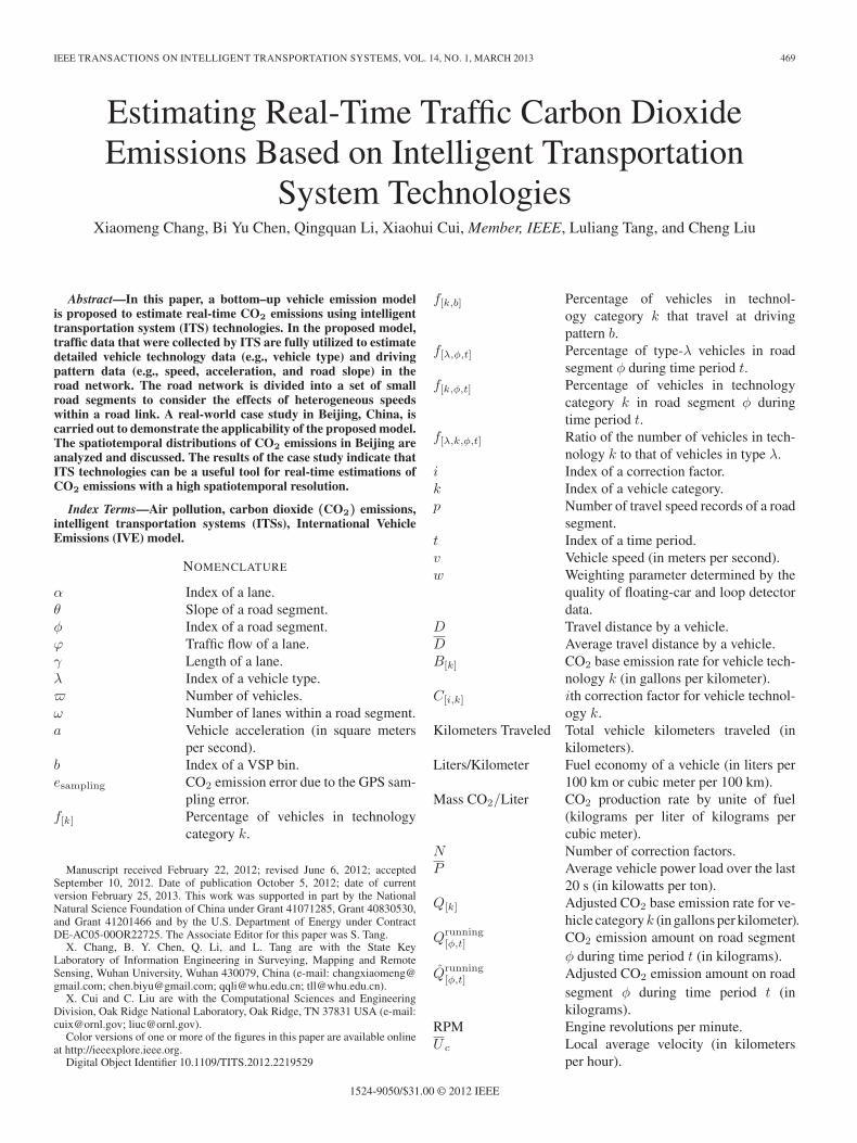
Fig. 1. Illustrative example for the GPS data interpolation.

where, XA, YA, and ZA, respectively, are the longitude, lat-itude, and altitude of tail node A and XB , YB , and ZB ,respectively, are the longitude, latitude, and altitude of headnode B.

B. Road-Segment Driving Pattern Distribution

Due to inevitable positioning errors caused by GPS receiversand geometric errors of the digital road network, the GPS datathat were collected by the floating-car system could not directlybe matched onto the real road network [26]. Therefore, rawGPS data need to be processed before being further used. In thispaper, a probabilistic analysis-based map-matching algorithmis employed to match the low-logging GPS data onto the roadnetwork [34].

As aforementioned, the GPS data collected by the floating-car system tend to have low frequency (e.g., 20 s). In this paper,available low-frequent GPS data are interpolated into second-by-second speed profiles to calculate the VSP and ES binsin (2)–(5). A cubic spline interpolation method is adopted.Fig. 1 gives an illustrative example of this GPS data inter-polation. In this figure, the black line refers to the actualhigh-frequent GPS data, whereas the red line refers to the inter-polated GPS data. It is shown that the cubic spline interpolationmethod can provide a reasonable approximation of the actualhigh-frequent GPS data. It is also shown in Fig. 1 that, using thiscubic spline interpolation method, some detailed accelerationor deceleration information may be missed, thus resulting inan underestimation of CO2 emissions. The estimation error dueto low-frequent GPS data should be taken into account in theproposed model (refer to Section III-D).

The second-by-second GPS data of all probe vehicles arethen matched to road segments. For each road segment andeach probe vehicle, VSP and ES bin values be calculated using(2)–(5). It is assumed in this paper that the driving patterns(speed, acceleration, and road slope) of probe vehicles canrepresent those of all vehicles on the same road segment duringa short time interval. This assumption seems valid in the con-gested urban road network, where vehicles do not have muchfreedom to change their travel speeds. Using this assumption,the driving pattern distribution, which is denoted by f[b,k,φ,t],could be obtained for each road segment φ and time period t.

C. Road-Segment Vehicle Kilometers Traveled

In the proposed model, the traffic flow data (i.e., total numberof passing vehicles) collected by loop detectors are employed to


calculate the vehicle kilometers traveled (denoted by V KT[φ,t])for road segment φ and time period t.

The loop detectors can observe the traffic flows for each lane.Because the lane lengths for some links with a horizontal curveare not identical, the vehicle kilometers traveled are calculatedby lanes in this paper. Let ω[φ] be the number of lanes within theroad segment φ and γα

[φ] be the length of its αth lane. V KT[φ,t]

can be calculated by

V KT[φ,t] =∑ω[φ]

(ϕα[φ,t] · γα

[φ]

)(9)

where ϕα[φ,t] is the traffic flow of the αth lane within segment φ

during time period t.

D. Road-Segment Vehicle Technology Distribution

Let f[k,φ,t] be the vehicle percentage in technology categoryk in road segment φ during time period t. To obtain this vehicletechnology distribution parameter, detailed vehicle technolo-gies (e.g., vehicle type, engine sizes, fuel types, and vehicleages) for all vehicles in the road segment are required. Theloop detector data can be very useful for identifying the types ofvehicles that pass through the road segment, including privatecars, buses, trucks, and motorcycles [35]–[37]. In this case, thepercentage of type λ vehicles in road segment φ during timeperiod t (denoted by f[λ,φ,t]) can be obtained from the loopdetector data. Then, f[k,φ,t] can be calculated by

f[k,φ,t] = f[λ,φ,t] · f[λ,k,φ,t]λ ∈{private cars, buses, trucks,motorcycles, etc.}

(10)

where f[λ,k,φ,t] is the ratio of the number of vehicles in technol-ogy k to that of vehicles in type λ. The f[λ,k,φ,t] parameter canbe obtained by the roadside survey, which can be conducted ona regular period (e.g., each year).

E. Segment-Based Vehicle Emission Model

According to the aforementioned road-segment formulation,the CO2 emissions by road segment (denoted by Qrunning

[φ,t] ) canbe calculated by

Qrunning[φ,t] =

UFTP · V KT[φ,t]

U [φ,t]

·∑λ

1372∑k=1

60∑b=1

(f[λ,φ,t] · f[λ,k,φ,t] · f[k,b,φ,t] · C[k,b] ·Q[k]

)

(11)

where U [φ,t] is the average vehicle speed in road segment φduring time period t. This U [φ,t] value can be calculated byfusing the travel speed that was estimated by both floating-carand loop detector data by

U [φ,t] = (1 − w) · UGPS[φ,t] + w · ULoop

[φ,t] (12)

where UGPS[φ,t] is the travel speed that was estimated by GPS

data from the floating-car system, ULoop[φ,t] is travel speed that

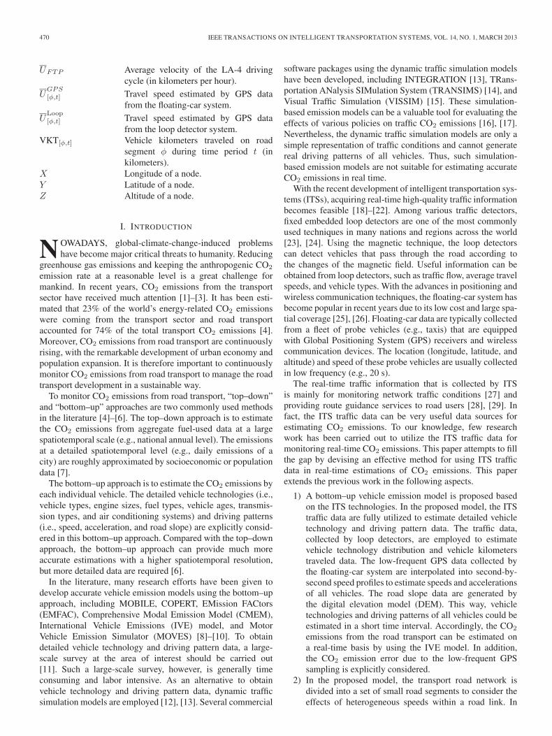
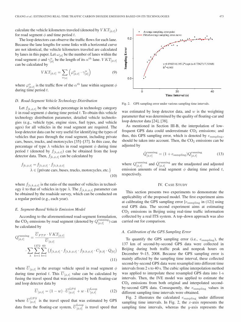
Fig. 2. GPS sampling error under various sampling time intervals.

was estimated by loop detector data, and w is the weightingparameter that was determined by the quality of floating-car andloop detector data [24], [38].

As mentioned in Section III-B, the interpolation of low-frequent GPS data could underestimate CO2 emissions; andthus, this GPS sampling error, which is denoted by esampling,should be taken into account. Then, the CO2 emissions can beadjusted by

Q̂running[φ,t] = (1 + esampling)Q

running[φ,t] (13)

where Qrunning[φ,t] and Q̂running

[φ,t] are the unadjusted and adjustedemission amounts of road segment φ during time period t,respectively.

IV. CASE STUDY

This section presents two experiments to demonstrate theapplicability of the proposed model. The first experiment aimsat calibrating the GPS sampling error [esampling in (12)] usingreal GPS data. The second experiment aims at estimatingCO2 emissions in Beijing using real-time traffic informationcollected by a real ITS system. A top–down approach was alsocarried out for comparison.

A. Calibration of the GPS Sampling Error

To quantify the GPS sampling error (i.e., esampling), the137 km of second-by-second GPS data were collected inBeijing during both traffic peak and nonpeak hours onDecember 9–15, 2008. Because the GPS sampling error ismainly affected by the sampling time interval, these collectedsecond-by-second GPS data were resampled into different timeintervals from 2 s to 40 s. The cubic spline interpolation methodwas applied to interpolate these resampled GPS data into 1-sintervals. Then, the IVE model was applied to estimate theCO2 emissions from both original and interpolated second-by-second GPS data. Consequently, the esampling values indifferent sampling time intervals were obtained.

Fig. 2 illustrates the calculated esampling under differentsampling time intervals. In Fig. 2, the x-axis represents thesampling time intervals, whereas the y-axis represents the


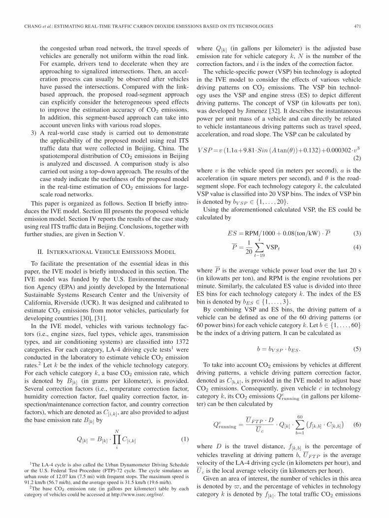
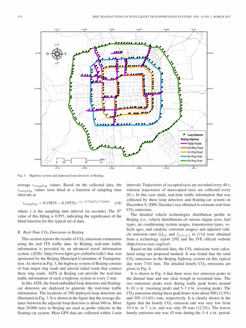
Fig. 3. Highway system and deployed loop detectors in Beijing.

average esampling values. Based on the collected data, theesampling values were fitted as a function of sampling timeintervals as

esampling = 0.19835 − 0.19532e−(x−0.72427)/7.33568 (14)

where x is the sampling time interval (in seconds). The R2

value of this fitting is 0.955, indicating the significance of thefitted function for this typical set of data.

B. Real-Time CO2 Emissions in Beijing

This section reports the results of CO2 emissions estimationsusing the real ITS traffic data. In Beijing, real-time trafficinformation is provided by an advanced travel informationsystem (ATIS) (http://www.bjjtw.gov.cn/bmfw/sslk/) that wassponsored by the Beijing Municipal Committee of Transporta-tion. As shown in Fig. 3, the highway system of Beijing consistsof four major ring roads and arterial radial roads that connectthese ring roads. AITS in Beijing can provide the real-timetraffic information of such a highway system in every 2 min.

In this ATIS, the fixed embedded loop detectors and floating-car detectors are deployed to generate the real-time trafficinformation. The locations of 390 deployed loop detectors areillustrated in Fig. 3. It is shown in the figure that the average dis-tance between the adjacent loop detectors is about 940 m. Morethan 20 000 taxis in Beijing are used as probe vehicles in thefloating-car system. Most GPS data are collected within 1-min

intervals. Trajectories of occupied taxis are recorded every 40 s,whereas trajectories of unoccupied taxis are collected every20 s. In this case study, real-time traffic information that wascollected by these loop detectors and floating-car system onDecember 9, 2008 (Tuesday) was obtained to estimate real-timeCO2 emissions.

The detailed vehicle technologies distribution profile inBeijing (i.e., vehicle distributions of various engine sizes, fueltypes, air conditioning system usages, transmission types, ve-hicle ages, and catalytic converter usages) and adjusted vehi-cle emission rates [Q[k] and f[λ,k,φ,t] in (11)] were obtainedfrom a technology report [39] and the IVE official website(http://www.issrc.org/ive/).

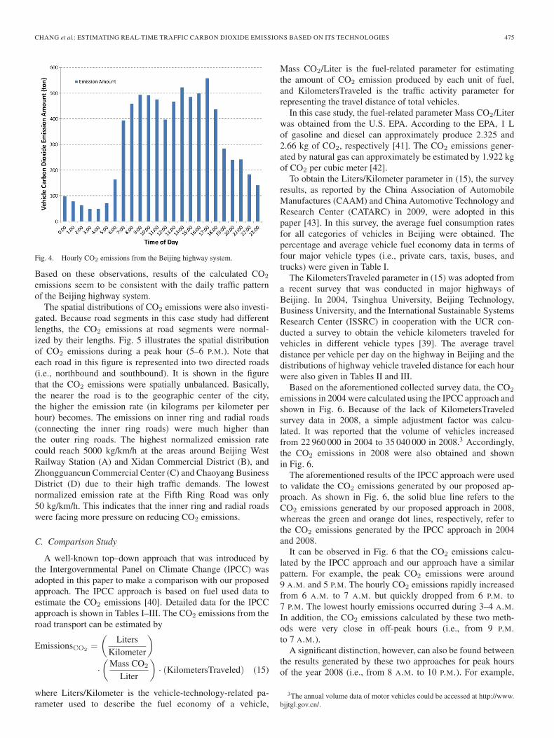
Based on the collected data, the CO2 emissions were calcu-lated using our proposed method. It was found that the totalCO2 emissions in the Beijing highway system on this typicalday were 7341 tons. The detailed hourly CO2 emissions aregiven in Fig. 4.

It is shown in Fig. 4 that there were two emission peaks inthe diurnal time and one clear trough in nocturnal time. Thetwo emissions peaks were during traffic peak hours around8–10 A.M. (morning peak) and 5–7 P.M. (evening peak). TheCO2 emissions during these peak hours were about 500 (12.9%)and 550 (13.6%) tons, respectively. It is clearly shown in thefigure that the hourly CO2 emission rate was very low from10 P.M. to 7 A.M. and was only 99 tons (12.2%). The lowesthourly emission rate was 45 tons during the 3–4 A.M. period.


Fig. 4. Hourly CO2 emissions from the Beijing highway system.

Based on these observations, results of the calculated CO2

emissions seem to be consistent with the daily traffic patternof the Beijing highway system.

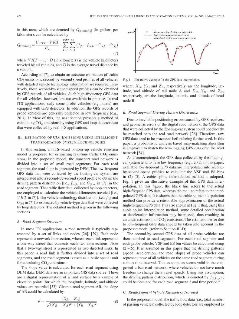
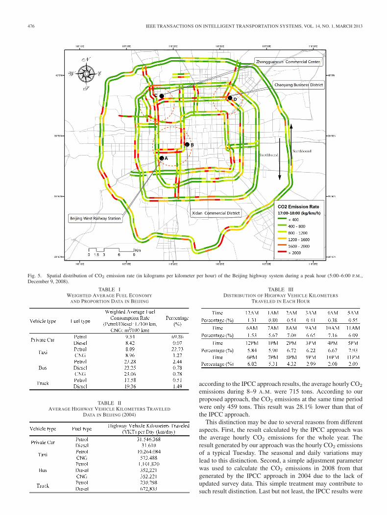
The spatial distributions of CO2 emissions were also investi-gated. Because road segments in this case study had differentlengths, the CO2 emissions at road segments were normal-ized by their lengths. Fig. 5 illustrates the spatial distributionof CO2 emissions during a peak hour (5–6 P.M.). Note thateach road in this figure is represented into two directed roads(i.e., northbound and southbound). It is shown in the figurethat the CO2 emissions were spatially unbalanced. Basically,the nearer the road is to the geographic center of the city,the higher the emission rate (in kilograms per kilometer perhour) becomes. The emissions on inner ring and radial roads(connecting the inner ring roads) were much higher thanthe outer ring roads. The highest normalized emission ratecould reach 5000 kg/km/h at the areas around Beijing WestRailway Station (A) and Xidan Commercial District (B), andZhongguancun Commercial Center (C) and Chaoyang BusinessDistrict (D) due to their high traffic demands. The lowestnormalized emission rate at the Fifth Ring Road was only50 kg/km/h. This indicates that the inner ring and radial roadswere facing more pressure on reducing CO2 emissions.

C. Comparison Study

A well-known top–down approach that was introduced bythe Intergovernmental Panel on Climate Change (IPCC) wasadopted in this paper to make a comparison with our proposedapproach. The IPCC approach is based on fuel used data toestimate the CO2 emissions [40]. Detailed data for the IPCCapproach is shown in Tables I–III. The CO2 emissions from theroad transport can be estimated by

EmissionsCO2=

(Liters

Kilometer

)

·(

Mass CO2

Liter

)· (KilometersTraveled) (15)

where Liters/Kilometer is the vehicle-technology-related pa-rameter used to describe the fuel economy of a vehicle,

Mass CO2/Liter is the fuel-related parameter for estimatingthe amount of CO2 emission produced by each unit of fuel,and KilometersTraveled is the traffic activity parameter forrepresenting the travel distance of total vehicles.

In this case study, the fuel-related parameter Mass CO2/Literwas obtained from the U.S. EPA. According to the EPA, 1 Lof gasoline and diesel can approximately produce 2.325 and2.66 kg of CO2, respectively [41]. The CO2 emissions gener-ated by natural gas can approximately be estimated by 1.922 kgof CO2 per cubic meter [42].

To obtain the Liters/Kilometer parameter in (15), the surveyresults, as reported by the China Association of AutomobileManufactures (CAAM) and China Automotive Technology andResearch Center (CATARC) in 2009, were adopted in thispaper [43]. In this survey, the average fuel consumption ratesfor all categories of vehicles in Beijing were obtained. Thepercentage and average vehicle fuel economy data in terms offour major vehicle types (i.e., private cars, taxis, buses, andtrucks) were given in Table I.

The KilometersTraveled parameter in (15) was adopted froma recent survey that was conducted in major highways ofBeijing. In 2004, Tsinghua University, Beijing Technology,Business University, and the International Sustainable SystemsResearch Center (ISSRC) in cooperation with the UCR con-ducted a survey to obtain the vehicle kilometers traveled forvehicles in different vehicle types [39]. The average traveldistance per vehicle per day on the highway in Beijing and thedistributions of highway vehicle traveled distance for each hourwere also given in Tables II and III.

Based on the aforementioned collected survey data, the CO2

emissions in 2004 were calculated using the IPCC approach andshown in Fig. 6. Because of the lack of KilometersTraveledsurvey data in 2008, a simple adjustment factor was calcu-lated. It was reported that the volume of vehicles increasedfrom 22 960 000 in 2004 to 35 040 000 in 2008.3 Accordingly,the CO2 emissions in 2008 were also obtained and shownin Fig. 6.

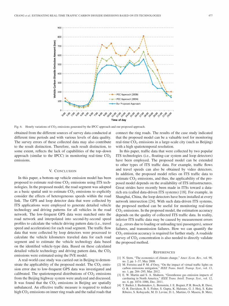
The aforementioned results of the IPCC approach were usedto validate the CO2 emissions generated by our proposed ap-proach. As shown in Fig. 6, the solid blue line refers to theCO2 emissions generated by our proposed approach in 2008,whereas the green and orange dot lines, respectively, refer tothe CO2 emissions generated by the IPCC approach in 2004and 2008.

It can be observed in Fig. 6 that the CO2 emissions calcu-lated by the IPCC approach and our approach have a similarpattern. For example, the peak CO2 emissions were around9 A.M. and 5 P.M. The hourly CO2 emissions rapidly increasedfrom 6 A.M. to 7 A.M. but quickly dropped from 6 P.M. to7 P.M. The lowest hourly emissions occurred during 3–4 A.M.In addition, the CO2 emissions calculated by these two meth-ods were very close in off-peak hours (i.e., from 9 P.M.to 7 A.M.).

A significant distinction, however, can also be found betweenthe results generated by these two approaches for peak hoursof the year 2008 (i.e., from 8 A.M. to 10 P.M.). For example,

3The annual volume data of motor vehicles could be accessed at http://www.bjjtgl.gov.cn/.


Fig. 5. Spatial distribution of CO2 emission rate (in kilograms per kilometer per hour) of the Beijing highway system during a peak hour (5:00–6:00 P.M.,December 9, 2008).

TABLE IWEIGHTED AVERAGE FUEL ECONOMY

AND PROPORTION DATA IN BEIJING

TABLE IIAVERAGE HIGHWAY VEHICLE KILOMETERS TRAVELED

DATA IN BEIJING (2004)

TABLE IIIDISTRIBUTION OF HIGHWAY VEHICLE KILOMETERS

TRAVELED IN EACH HOUR

according to the IPCC approach results, the average hourly CO2

emissions during 8–9 A.M. were 715 tons. According to ourproposed approach, the CO2 emissions at the same time periodwere only 459 tons. This result was 28.1% lower than that ofthe IPCC approach.

This distinction may be due to several reasons from differentaspects. First, the result calculated by the IPCC approach wasthe average hourly CO2 emissions for the whole year. Theresult generated by our approach was the hourly CO2 emissionsof a typical Tuesday. The seasonal and daily variations maylead to this distinction. Second, a simple adjustment parameterwas used to calculate the CO2 emissions in 2008 from thatgenerated by the IPCC approach in 2004 due to the lack ofupdated survey data. This simple treatment may contribute tosuch result distinction. Last but not least, the IPCC results were


Fig. 6. Hourly variations of CO2 emissions generated by the IPCC approach and our proposed approach.

obtained from the different sources of survey data conducted atdifferent time periods and with various levels of data quality.The survey errors of these collected data may also contributeto the result distinction. Therefore, such result distinction, tosome extent, reflects the lack of capabilities of the top–downapproach (similar to the IPCC) in monitoring real-time CO2

emissions.

V. CONCLUSION

In this paper, a bottom–up vehicle emission model has beenproposed to estimate real-time CO2 emissions using ITS tech-nologies. In the proposed model, the road segment was adoptedas a basic spatial unit to estimate CO2 emissions to explicitlyconsider the effects of heterogeneous speeds within the roadlink. The GPS and loop detector data that were collected byITS applications were employed to generate detailed vehicletechnology and driving patterns for all vehicles in the roadnetwork. The low-frequent GPS data were matched onto theroad network and interpolated into second-by-second speedprofiles to calculate the vehicle driving pattern data (i.e., travelspeed and acceleration) for each road segment. The traffic flowdata that were collected by loop detectors were processed tocalculate the vehicle kilometers traveled data for each roadsegment and to estimate the vehicle technology data basedon the identified vehicle-type data. Based on these calculateddetailed vehicle technology and driving pattern data, the CO2

emissions were estimated using the IVE model.A real-world case study was carried out in Beijing to demon-

strate the applicability of the proposed model. The CO2 emis-sion error due to low-frequent GPS data was investigated andcalibrated. The spatiotemporal distributions of CO2 emissionsfrom the Beijing highway system were analyzed and discussed.It was found that the CO2 emissions in Beijing are spatiallyunbalanced. An effective traffic measure is required to reducehigh CO2 emissions on inner ring roads and the radial roads that

connect the ring roads. The results of the case study indicatedthat the proposed model can be a valuable tool for monitoringreal-time CO2 emissions in a large-scale city (such as Beijing)with a high spatiotemporal resolution.

In this paper, traffic data that were collected by two popularITS technologies (i.e., floating-car system and loop detectors)have been employed. The proposed model can be extendedto other types of ITS traffic data. For example, traffic flowsand travel speeds can also be obtained by video detectors.In addition, the proposed model relies on ITS traffic data toestimate CO2 emissions, and thus, the applicability of the pro-posed model depends on the availability of ITS infrastructures.Great strides have recently been made in ITSs toward a data-rich era (called data-driven ITS systems) [18]. For example, inShanghai, China, the loop detectors have been installed at everynetwork intersection [24]. With such data-driven ITS systems,the proposed method can be useful for monitoring real-timeCO2 emissions. In the proposed model, the estimation accuracydepends on the quality of collected ITS traffic data. In reality,inferior ITS traffic data may be caused by measurement errors(e.g., errors due to loading or unloading taxi passengers), sensorfailures, and transmission failures. How we can quantify theCO2 emission accuracy is required for further study. A roadsidesurvey of CO2 concentration is also needed to directly validatethe proposed method.

REFERENCES

[1] N. Stern, “The economics of climate change,” Amer. Econ. Rev., vol. 98,no. 2, pp. 1–37, May 2008.

[2] M. Ferreira and P. M. d’Orey, “On the impact of virtual traffic lights oncarbon emissions mitigation,” IEEE Trans. Intell. Transp. Syst., vol. 13,no. 1, pp. 284–295, Mar. 2012.

[3] E. W. Martin and S. A. Shaheen, “Greenhouse gas emission impacts ofcarsharing in North America,” IEEE Trans. Intell. Transp. Syst., vol. 12,no. 4, pp. 1074–1086, Dec. 2011.

[4] T. Barker, I. Bashmakov, L. Bernstein, J. E. Bogner, P. R. Bosch, R. Dave,O. R. Davidson, B. S. Fisher, S. Gupta, K. Halsnæs, G. J. Heij, S. KahnRibeiro, S. Kobayashi, M. D. Levine, D. L. Martino, O. Masera, B. Metz,


L. A. Meyer, G.-J. Nabuurs, A. Najam, N. Nakicenovic, H.-H. Rogner,J. Roy, J. Sathaye, R. Schock, P. Shukla, R. E. H. Sims, P. Smith,D. A. Tirpak, D. Urge-Vorsatz, and D. Zhou, Climate Change 2007:Mitigation. Contribution of Working Group III to the Fourth AssessmentReport of the Intergovernmental Panel on Climate Change. Cambridge,U.K.: Cambridge Univ. Press, 2007.

[5] D. P. Van Vuuren, M. Hoogwijk, T. Barker, K. Riahi, S. Boeters,J. Chateau, S. Scrieciu, J. Van Vliet, T. Masui, K. Blok, E. Blomen, andT. Kram, “Comparison of top–down and bottom–up estimates of sectoraland regional greenhouse gas emission reduction potentials,” Energy Pol-icy, vol. 37, no. 12, pp. 5125–5139, Dec. 2009.

[6] A. Namdeo, G. Mitchell, and R. Dixon, “TEMMS: An integrated pack-age for modeling and mapping urban traffic emissions and air quality,”Environ. Modell. Softw., vol. 17, no. 2, pp. 177–188, 2002.

[7] H. Cai and S. D. Xie, “Estimation of vehicular emission inventories inChina from 1980 to 2005,” Atmos. Environ., vol. 41, no. 39, pp. 8963–8979, Dec. 2007.

[8] P. Sharma and M. Khare, “Modeling of vehicular exhausts—A review,”Transp. Res. D: Transp. Environ., vol. 6, no. 3, pp. 179–198, May 2001.

[9] H. Rakha, K. Ahn, and A. Trani, “Comparison of MOBILE5a, MOBILE6,VT-MICRO, and CMEM models for estimating hot-stabilized light-dutygasoline vehicle emissions,” Can. J. Civ. Eng., vol. 30, no. 6, pp. 1010–1021, Dec. 2003.

[10] S. Abo-Qudais and H. Qdais, “Performance evaluation of vehicles emis-sions prediction models,” Clean Technol. Environ. Policy, vol. 7, no. 4,pp. 279–284, Nov. 2005.

[11] H. Liu, K. B. He, Q. D. Wang, H. Huo, J. Lents, N. Davis, N. Nikkila,C. H. Chen, M. Osses, and C. Y. He, “Comparison of vehicle activitybetween Beijing and Shanghai,” J. Air Waste Manage. Assoc., vol. 57,no. 10, pp. 1172–1177, Oct. 2007.

[12] Q. Q. Li, X. M. Chang, X. H. Cui, L. L. Tang, Z. H. Li, and C. Liu, “Road-segment-based vehicle emission model for real-time traffic greenhousegas estimation,” presented at the Transp. Res. Board 90th Annu. Meet.,Washington, DC, Jan. 23–27, 2011, Paper 11-1774.

[13] H. Rakha and K. Ahn, “Integration modeling framework for estimatingmobile source emissions,” J. Transp. Eng., vol. 130, no. 2, pp. 183–193,Mar. 2004.

[14] J. Zietsman and L. R. Rilett, “Analysis of aggregation bias in vehicu-lar emission estimation using TRANSIMS output,” Transp. Res. Rec.,vol. 1750, pp. 56–63, 2001.

[15] VISSIM 4.10 User Manual, PTV Planung Transport Verkehr AG,Karlsruhe, Germany, 2005.

[16] R. X. Zhong, A. Sumalee, and T. Maruyamab, “Dynamic marginalcost, access control, and pollution charge: A comparison of bottleneckand whole link models,” J. Adv. Transp., vol. 46, no. 3, pp. 191–221,Jul. 2012.

[17] Z.-C. Li, W. H. K. Lam, S. C. Wong, and A. Sumalee, “Environmentallysustainable toll design for congested road networks with uncertain de-mand,” Int. J. Sustain. Transp., vol. 6, no. 3, pp. 127–155, May 2012.

[18] J. P. Zhang, F. Y. Wang, K. F. Wang, W. H. Lin, X. Xu, and C. Chen,“Data-driven intelligent transportation systems: A survey,” IEEE Trans.Intell. Transp. Syst., vol. 12, no. 4, pp. 1624–1639, Dec. 2011.

[19] F. Soriguera and F. Robuste, “Requiem for freeway travel time estimationmethods based on blind speed interpolations between point measure-ments,” IEEE Trans. Intell. Transp. Syst., vol. 12, no. 1, pp. 291–297,Mar. 2011.

[20] S. L. Sun and X. Xu, “Variational inference for infinite mixtures ofGaussian processes with applications to traffic flow prediction,” IEEETrans. Intell. Transp. Syst., vol. 12, no. 2, pp. 466–475, Jun. 2011.

[21] Y. F. Yuan, J. W. C. van Lint, R. E. Wilson, F. van Wageningen-Kessels,and S. P. Hoogendoorn, “Real-time Lagrangian traffic state estimator forfreeways,” IEEE Trans. Intell. Transp. Syst., vol. 13, no. 1, pp. 59–70,Mar. 2012.

[22] C. van Hinsbergen, T. Schreiter, F. S. Zuurbier, J. W. C. van Lint, andH. J. van Zuylen, “Localized extended Kalman filter for scalable real-timetraffic state estimation,” IEEE Trans. Intell. Transp. Syst., vol. 13, no. 1,pp. 385–394, Mar. 2012.

[23] W. H. K. Lam, Y. F. Tang, K. S. Chan, and M. L. Tam, “Short-term hourlytraffic forecasts using Hong Kong annual traffic census,” Transp., vol. 33,no. 3, pp. 291–310, May 2006.

[24] Q. J. Kong, Z. P. Li, Y. K. Chen, and Y. C. Liu, “An approach to urbantraffic state estimation by fusing multisource information,” IEEE Trans.Intell. Transp. Syst., vol. 10, no. 3, pp. 499–511, Sep. 2009.

[25] H. Zou, Y. Yue, Q. Li, and A. G. O. Yeh, “An improved distance metricfor the interpolation of link-based traffic data using kriging: A case studyof a large-scale urban road network,” Int. J. Geograph. Inf. Sci., vol. 26,no. 4, pp. 667–689, Apr. 2012.

[26] Q. Li, T. Zhang, and Y. Yu, “Using cloud computing to process intensivefloating-car data for urban traffic surveillance,” Int. J. Geograph. Inf. Sci.,vol. 25, no. 8, pp. 1303–1322, Aug. 2011.

[27] M. L. Tam and W. H. K. Lam, “Using automatic vehicle identificationdata for travel time estimation in Hong Kong,” Transportmetrica, vol. 4,no. 3, pp. 179–194, Sep. 2008.

[28] B. Y. Chen, W. H. K. Lam, A. Sumalee, and Z.-L. Li, “Reliableshortest path finding in stochastic networks with spatial correlated linktravel times,” Int. J. Geograph. Inf. Sci., vol. 26, no. 2, pp. 365–386,Feb. 2012.

[29] B. Y. Chen, W. H. K. Lam, A. Sumalee, Q. Li, H. Shao, and X. Fang,“Finding reliable shortest paths in road networks under uncertainty,”Netw. Spatial Econ. DOI:10.1007/s11067-012-9175-1.

[30] N. Davis, J. Lents, M. Osses, N. Nikkila, and M. Barth, “Development andapplication of an international vehicle emissions model,” in Proc. 84thAnnu. Meet. Transp. Res. Board, 2005, vol. 1939, pp. 157–165.

[31] IVE Model User Manual, Int. Sustainable Syst. Res. Center, La Habra,CA, 2008.

[32] J. L. Jimenez, “Understanding and quantifying motor vehicle emissionswith vehicle specific power and TILDAS remote sensing,” Ph.D. disserta-tion, Mass. Inst. Technol., Cambridge, MA, 1999.

[33] J. A. Thompson, J. C. Bell, and C. A. Butler, “Digital elevationmodel resolution: Effects on terrain attribute calculation and quantita-tive soil-landscape modeling,” Geoderma, vol. 100, no. 1/2, pp. 67–89,Mar. 2001.

[34] W. Wang, J. Jin, B. Ran, and X. C. Guo, “Large-scale freeway networktraffic monitoring: A map-matching algorithm based on low-logging fre-quency GPS probe data,” J. Intell. Transp. Syst., vol. 15, no. 2, pp. 63–74,Apr. 2011.

[35] Y. H. Wang and N. L. Nihan, “Can single-loop detectors do the workof dual-loop detectors?” J. Transp. Eng., vol. 129, no. 2, pp. 169–176,Mar./Apr. 2003.

[36] Y. Wang and N. L. Nihan, “Dynamic estimation of freeway large-truckvolumes based on single-loop measurements,” J. Transp. Eng., vol. 8,no. 3, pp. 133–141, Jul. 2004.

[37] Y. K. Ki and D. K. Baik, “Vehicle-classification algorithm for single-loop detectors using neural networks,” IEEE Trans. Veh. Technol., vol. 55,no. 6, pp. 1704–1711, Nov. 2006.

[38] M. Dell’Orco and D. Teodorovic, “Data fusion for updating informationin modeling drivers’ choice behavior,” Transportmetrica, vol. 5, no. 2,pp. 107–123, 2009.

[39] H. H. Oliver, K. S. Gallagher, M. Li, K. Qin, J. Zhang, H. Li, andK. He, “In-use vehicle emissions in China: Beijing study,” EnergyTechnol. Innovation Policy Res. Group, Belfer Center Sci. Int. Affairs,Harvard Kennedy School, Cambridge, MA, Discussion Paper 2009-05,Mar. 2009.

[40] S. Holloway, A. Karimjee, M. Akai, R. Pipatti, and K. Rypdal, 2006 IPCCGuidelines for National Greenhouse Gas Inventories. Kanagawa, Japan:IGES, 2006, ch. 5.

[41] Emission Facts: Average Carbon Dioxide Emissions Resulting FromGasoline and Diesel Fuel, Environ. Protection Agency, Washington,DC, Feb. 2005. [Online]. Available: http://www.epa.gov/otaq/climate/420f05001.htm

[42] Inventory of U.S. Greenhouse Gas Emissions and Sinks: 1990–2008,EPA, Washington, DC. [Online]. Available: www.epa.gov/climatechange/emissions/usinventoryreport.html

[43] Vehicle Fuel Economy in China, China Assoc. Autom. Manuf. ChinaAutom. Technol. Res. Cent., Beijing, China. [Online]. Available: http://caam.org.cn/files/file/0906/zhyh.pdf

Xiaomeng Chang received the B.S. degree fromNanjing University of Information Science and Tech-nology (formerly Nanjing Institute of Meteorology),Nanjing, China, in 2008 and the M.S. degree in geo-graphic information systems from Wuhan University,Wuhan, China, in 2010. He is currently workingtoward the Ph.D. degree in photography and remotesensing with the State Key Laboratory of Informa-tion Engineering in Surveying, Mapping and RemoteSensing, Wuhan University.

From October 2010 to November 2011, he wasa Visiting Scholar for Cooperation Research with the Oak Ridge NationalLaboratory, Oak Ridge, TN, and the University of Tennessee, Knoxville.His research interests include intelligent transportation systems, GeographicInformation Systems for transportation, and atmospheric environments.


Bi Yu Chen received the B.S. degree in survey-ing and mapping engineering and the M.S. degreein geographical information science from WuhanUniversity, Wuhan, China, in 2003 and 2006, re-spectively, and the Ph.D. degree in transportationengineering from the Hong Kong Polytechnic Uni-versity, Kowloon, Hong Kong, in 2012.

He is currently a Lecturer and a PostdoctoralFellow with the State Key Laboratory of Informa-tion Engineering in Surveying Mapping and RemoteSensing, Wuhan University. His research interests

include intelligent transportation systems, transport geography, network reli-ability, and vulnerability modeling.

Qingquan Li received the M.S. degree in engi-neering and the Ph.D degree in photogrammetryand remote sensing from Wuhan University, Wuhan,China, in 1988 and 1998, respectively.

From 1988 to 1996, he was an Assistant Pro-fessor with Wuhan University, where he becamean Associate professor from 1996 to 1998 and hasbeen a Professor with the State Key Laboratoryof Information Engineering in Surveying, Mapping,and Remote Sensing since 1998. He is currently theExecutive Vice President of Wuhan University and

the Director of the Engineering Research Center for Spatiotemporal DataSmart Acquisition and Application, Ministry of Education of China. He isan expert in Modern Traffic with the National 863 Plan and an EditorialBoard Member of the Surveying and Mapping Journal and the Wuhan Uni-versity Journal—Information Science Edition. His research interests includephotogrammetry, remote sensing, and intelligent transportation systems.

Xiaohui Cui (M’02) received the B.S. degree fromWuhan Technical University of Surveying and Map-ping, Wuhan, China, in 1992, the M.S. degree fromWuhan University in 2000, and the Ph.D. degreefrom the University of Louisville, Louisville, KY,in 2004.

He is currently an Assistant Professor with theComputer Science Department, New York Instituteof Technology. Meanwhile, he has served as a StaffScientist with the Oak Ridge National Laboratoryof the Department of Energy, Oak Ridge, TN. His

research interests include swarm intelligence, GPU computing, agent-basedmodeling and simulation, cyber security, GIS and transportation, emergentbehavior, complex systems, high-performance computing, social computing,and information retrieval.

Dr. Cui is a member of the Association for Computing Machinery andthe North American Association for Computational Social and OrganizationalSciences.

Luliang Tang received the B.S. degree from WuhanTechnical University of Surveying and Mapping,Wuhan, China, in 1998 and the M.S. and Ph.D.degrees from Wuhan University in 2003 and 2007,respectively.

He is currently an Associate Professor with theState Key Laboratory for Information Engineeringin Surveying, Mapping and Remote Sensing, WuhanUniversity. His research interests include intelli-gent transportation systems, Geographic InformationSystems for transportation, and spatial data change

detecting.

Cheng Liu received the B.S. degree from theChinese Cultural University, Taipei, Taiwan, in 1974,the M.S. degree from Taiwan Normal University,Taipei, in 1976, and the Ph.D. degree from the Uni-versity of Tennessee, Knoxville, in 1986.

He is currently an Adjunct Associate Professorwith the Department of Geography, University ofTennessee and has served as a Staff Scientist with theOak Ridge National Laboratory, Oak Ridge, TN. Hisresearch interests include geographic informationsystems, operations research, transportation model-

ing, algorithm design, supply chain management, software development, andhigh-performance geocomputing.

estimating real-time traffic carbon dioxide emissions based on intelligent transportation system...

Documents