Estimating public values for marine protected areas in the northeast United States: a latent class modeling approach K. Wallmo and S. Edwards

U.S. Department of Commerce National Oceanic and Atmospheric Administration National Marine Fisheries Service NOAA Technical Memorandum NMFS-F/SPO-84 October 2007

Estimating public values for marine protected areas in the northeast United States: a latent class modeling approach K. Wallmo and S. Edwards NOAA Fisheries Office of Science and Technology NOAA Fisheries Northeast Fisheries Science Center NOAA Technical Memorandum NMFS-F/SPO-84 October 2007

U.S. Department of Commerce Carlos M. Gutiérrez, Secretary National Oceanic and Atmospheric Administration Vice Admiral Conrad C. Lautenbacher, Jr., USN (Ret.) Under Secretary for Oceans and Atmosphere National Marine Fisheries Service William T. Hogarth, Assistant Administrator for Fisheries

Suggested citation: Wallmo, K., and S. Edwards. 2007. Estimating public values for marine protected areas in the northeast United States: a latent class modeling approach. U.S. Dep. Of Commerce, NOAA Tech. Memo. NMFS-F/SPO-84, 75 p. A copy of this report may be obtained from: Office of Science and Technology NMFS, NOAA 1315 East-West Highway, F/ST5 Silver Spring, MD 20910

Summary Although popular with the environmental community for quite a while, the designation of the 362 thousand km2 Northwest Hawaiian Islands Marine National Monument in 2007 by President George W. Bush symbolizes the political ascension of Marine Protected Areas (MPAs) in the United States. MPAs are not panaceas for resource allocation, though (Degnbol et al. in press). The benefits of fishery reserves, in particular, are arguable. There is general agreement, however, that no-take ecological reserves are the most effective way to enhance and preserve the ecological diversity of marine species and their habitats on the sea floor. Scientific research indicates that 10%-40% of an ecosystem is required to preserve all species and their habitats. To insure against catastrophic events would require considerably more. But policy-makers must ask whether complete protection is too costly when compared to the opportunity costs of displaced activities. The zoning plans of MPAs generally exclude or substantially restrict many activities that are important to the economy and consumers, including commercial and recreational fishing, oil and natural gas production, sand and gravel mining, and clean renewable energy from windmills that require being attached to the sea floor. Debate over non-fungible objectives such as environmental protection and opportunity costs can be informed by adding the public’s valuation of ecological diversity. A person might value ecological reserves as a bequest to younger generations, or they might simply get personal satisfaction from knowing that a part of the environment exists in a natural state. Bequest value and existence value are a class of economic benefits not revealed by markets. Instead economists use surveys that describe hypothetical market-like situations to elicit valuations of an environmental good, service, or asset. The contingent choice class of non-market methods is ideally suited to collecting data on the non-use value of multi-attribute resources such as marine ecological reserves. This research presents estimates of non-market values of marine protected areas in the Northeast Region of the US. A random sample of over 1300 households in the Northeast Region was presented with sets of hypothetical alternatives which differed in terms of reserve size (5%-40%), compatible uses (No-Take, Science and Education, passive forms of Leisure and Tourism, pelagic Fishing), and personal costs ($10-$150) and asked to choose the bundle that they preferred. Answers from the 77% of responders were analyzed with a latent class specification of the random-utility-model (RUM) to objectively test for heterogeneous preferences. Three distinct latent classes were identified in the sample. Roughly half of the responders (48%) saw reserve size as a normal economic good with positive, but diminishing marginal utility. Compensating variation was maximized at $133 per-household per-year for this group when total reserve size was 27% of the EEZ and the areas could only be used for scientific and educational purposes. Another class was characterized by

1

negative utility from MPAs (28%), and the final class (24%) had an incongruous positive response to personal cost, i.e. paying more for reserve size the more costly it became, possibly due to hypothetical bias in the questionnaire or non-conforming preferences. The model was applied to estimate the publics’ valuation of the Habitat Areas of Particular Concern (HAPC) being considered by the New England Fishery Management Council for an amendment to its Essential Fish Habitat Omnibus Plan. Together, the seamounts, canyons, and diverse areas of the shelf comprise 5.2% of the EEZ in the region. Allowing scientific and educational uses doubled estimates of compensating variation by Class 1 (positive utility) responders from more than $50 to almost $110 depending on the status quo. In contrast, compensating variation for Class 3 (disutility) averaged -$40 for the No-Take alternative and increased to -$9 as more uses were allowed. The positive parameter on cost for Class 2 is intractable in this model. In addition to presenting the methodology and results in detail, the report addresses the need to control for heterogeneous preferences in contingent choice research, a benefit-cost analysis framework that accounts for non-use value, and the effect of operating and opportunity costs on scientists’ estimates of optimum reserve size.

2

Introduction In the first assessment of the state of the oceans in 35 years, the US Commission on Ocean Policy (2004) reported continued threats to resource sustainability, degradation of marine ecosystems, and unproductive competition for ocean space by traditional and new stakeholders. These persistent problems can be traced to defective governance and property rights arrangements that fail to allocate resources effectively. However, even a “perfect” institutional arrangement (whatever that might be) would be compromised by the dearth of information on the value of things not exchanged in markets. The NRC Panel on Integrated Environmental and Economic Accounting (NRC 1999) warned that ignorance of the size of the “non-market” economy biases measures of aggregate welfare in favor of markets, such as National Income and Product Accounts. Perhaps least known (and understood) are the “non-use” values – i.e., the personal satisfaction that people get from protecting the environment for the benefit of others, particularly subsequent generations or wildlife itself. Marine Protected Areas (MPAs) – especially ecological reserves -- are the leading vehicle for promoting “non-use” values in the ocean. In 2000 when President Clinton signed Executive Order 13158 Marine Protected Areas to “help protect the significant natural and cultural resources within the marine environment for the benefit of present and future generations” (EO 13158, 2000), less than 1% of U.S. territorial waters was part of an MPA (Kelleher 1999). However, pressure from environmental organizations worldwide has begun to take effect. For example, in the United States in 2007, President Bush created the largest MPA in the world – the 362 thousand km2 Northwest Hawaiian Islands Marine National Monument which takes up a third of the Insular-Pacific Hawaiian Large Marine Ecosystem, and is bigger than the combination of all the states in the Northeast Region. MPAs are used for three general purposes – fisheries management, protection of cultural resources, and preservation of species and habitat diversity. There is scientific evidence that closing an area to extractive uses can rebuild fish stocks inside the area (Palumbi 2002; Halpern 2003; Roberts 2005), but scientists (Hilborn et al. 2004) and conservationists (Agardy 2005) are less sanguine about the overall benefit of fishery reserves. Similarly, economists point out that even fishery reserves that are successful from a biological standpoint could still fail on economic grounds if there is sufficient excess capacity to dissipate resource rents (Hannesson 1999). In large measure, the economic value of fishery reserves depends primarily on whether any net gains in the fishery from the migration of fish from inside the protected area is greater than the opportunity costs of closing the area (Sanchirico 2004). While the utility of fishery reserves is in doubt, there appears to be a consensus among scientists that MPAs are the only viable way to protect habitat and conserve biodiversity (Hilborn et al. 2004, Lubchenco et al. 2003; NRC 2001; Lauck et al. 1998; Scientific Consensus Statement on Marine Reserves and Marine Protected Areas 2001). The main objective of the MPA Federal Advisory Committee (Anonymous 2005; p. 4) is “conserving, enhancing, and/or restoring marine biodiversity … [and] … representative

3

examples of the nation’s marine habitats, as well as unique biophysical and geological features”. However, the committee also highlights the objective of “[p]roviding both appropriate access to and use of marine resources within MPAs consistent with the goals and objectives of the MPA” (p. 4). Scientists estimate that 10%-40% of a marine ecosystem (depending on its characteristics) would have to be set aside to preserve all ecological diversity (NRC 2001). The percentage can increase substantially to insure against the risk of catastrophe from oil spills, fishing gear, storms, and introduced species (Allison et al. 2003; Halpern 2003). From a policy standpoint, however, the question is not so much “how much is enough?” (Lubchenco et al. 2003), but “how much is too much?”. There are costs associated with displaced activities, such as the value of forgone energy and seafood. MPAs could not possibly be designed without scientific data, but E.O. 13158 is a public policy imbued with subjectivity about humans place in marine ecosystems, not an experiment. It is therefore legitimate to inquire about the public’s valuation of ecological reserves and the appropriate mix of protected areas and exploited areas. Even if someone does not expect to ever experience the sea floor first-hand, (s)he might value ecological reserves as a bequest to younger generations (bequest value) or for the knowledge that a part of the environment exists in a natural state (existence value). Together, these values are called non-use values. The contingent choice class of non-market methods is ideally suited to researching the non-use value of ecological reserves. Non-use values are, by definition, neither directly nor indirectly revealed in market data or by household production behavior (e.g., travel costs used as the price of a fishing trip); therefore, data can only be collected from a survey. In addition, the contingent choice method is designed to collect data on the attributes of a multi-characteristic commodity, such as ecological reserves. Data were collected from a survey of households in the Northeast Region of the US (for this research the Northeast Region refers to the states of Maine, New Hampshire, Massachusetts, Rhode Island, Connecticut, New York, New Jersey, Delaware, Maryland, and Virginia) to test the hypothesis that individuals have preferences not only for the size of an ecological reserve, but also for different types of uses of the reserve. Model results and estimates of non-use value are presented and discussed in the main text. Appendices present the questionnaire, summarize the survey data, and report test results for sampling and selection biases. This research project was funded jointly by the Economics and Social Sciences Division and the Habitat Division of NOAA Fisheries’ headquarters. We are grateful for the support of these divisions, and the patience of their chiefs – Dr. Rita Curtis (Economics and Social Sciences) and Mr. Thomas Bigford (Habitat) – and Kathi Rodrigues (Habitat).

4

Related Research The economics literature on the non-market benefits of MPAs is meager, says virtually nothing about non-use values, and cannot address questions about reserve size or allowable uses. Most of the literature reports estimates of the use-value of marine recreation, such as diving and snorkeling. In a contingent valuation study, Wielgus et al. (2003) found that divers were willing to pay US$2.60 per dive for a marginal improvement in coral and fish diversity at Eilat coral reefs in Israel. Using a similar methodology, divers at the Turks and Caicos Islands reportedly valued large increases in the size and abundance of Nassau grouper at US$50 (Rudd, Gore, and Tupper 2000). Other studies found that international tourists in the Seychelles were willing to pay about US$12 on average to prevent coral reef degradation in Seychelles’ marine parks (Mathieu et al. 2003). Arin and Kramer (2002) found that protecting coral reefs in the Philippines for local and international divers could generate revenues ranging from several thousand dollars a year up to one million, depending on the location of the coral reef being protected. Leeworthy (1991) reported estimates of divers’ willingness-to-pay ranging between $356 and $533 for trips to coral reefs in the Florida Keys National Marine Sanctuary. For comparison, Bhat (2003) estimates that, under the current quality conditions, trip values for diving, snorkeling, and glass-bottom boating also in the Florida Keys are about $463. The same study suggests that with significant improvements in fish abundance, visibility, and coral quality, the per-trip value would increase by 69%. Estimates of non-use values for MPAs are rare, but what exist are not applicable to US policy either because they are site-specific and carried out overseas, responders were visitors and local residents instead of the general public, or they are outdated (Davis 2003). Of the studies that do exist, Bennett (1984) reported that in 1979 local visitors to the coastal Nadgee Nature Reserve in New South Wales, Australia, were willing to pay an average of US$3 a year in perpetuity to preserve the park’s existence. Spash et al. (2000) reported that locals and tourists surveyed during 1998 were willing to pay US$1.17 and US$4.26 annually for five years for the uncertain proposition that money in a trust fund would support ways to improve marine biodiversity by 25% on coral reefs in Montego Bay, Jamaica. There are also a limited number of studies in the field of environmental and natural resource economics that have used the latent class estimator to test for heterogeneous preferences. The contingent valuation study of endangered species by Aldrich et al. (2007) is noteworthy because our results are qualitatively similar. In addition to improving model fit, they identified three classes of responders with very strong preferences for preservation, moderate preferences, or disutility. Conventional practice would combine these groups with structurally different preferences, which could lead to incorrect inferences, or address the differences through a priori specifications of the demand function or through the use of random parameters models (Morey 1993; Layton 1996). Our study extends the literature in several ways. First, it is one of the first studies of the non-use value of preserving species and habitat diversities in a large marine ecosystem.

5

Second, we are unaware of any other study that has estimated the economic value of an MPA as a function of the policy-relevant attributes, size and allowable uses. Finally, as just mentioned, our research contributes to the limited though growing use of latent class models for the valuation of environmental goods and services, and underscores the benefits, particularly for policy questions, of more flexible models (see Boxall and Adamowicz 2002). Survey Design Questionnaire development: The questionnaire was developed during January to September 2005 when three focus groups, three sets of cognitive interviews, and two pilot tests were conducted. Three challenges cropped up during these meetings. First, it became clear from the first focus group that managing the information effects in the survey would be a critical issue, as most participants had heard of the term marine protected area but had quite different views and understandings of what they are and why they are established. Further, many participants in focus groups associated coral reefs or other warm water habitats with MPAs. Thus one of the first challenges in survey design was to clearly communicate to responders what the primary purpose of the MPAs discussed in the survey would be. We stressed at several different points in the survey that the benefits of the MPAs would include (1) the protection of habitat and marine life diversity on the sea floor in the Northeast Region, and (2) the prevention of industrial development, such as drilling for oil or gas, within the MPA boundaries. Any other benefits would be incidental at best (e.g., protection of migratory species). A second challenge was to convey in clear and concise text the findings from the scientific literature about reserve size. This was difficult, as many of the findings do not enjoy consensus among all scientists, and even when they do they are often case or site-specific. Ultimately we relied on wordsmithing the NRC (2001) report which summarized the views of thirteen marine scientists on the relationship between reserve size and preservation of ecological diversity. A third challenge was ensuring that we presented balanced information on both the potential benefits and costs of MPAs. This was particularly important since MPAs are a relatively contentious in the northeastern US, due in part to strong ties to fishing and other marine related industries. Not surprisingly, all three focus groups contained participants who, prior to the focus group, either strongly supported or opposed MPAs, and thus it was important that the information in the survey was presented neutrally. We felt that the benefits were aptly described by communicating the purpose of the MPAs, e.g. protecting habitat and diversity on the sea floor, and the relationship between reserve size and diversity summarized by the NRC. To balance that information we developed a section of the survey that described the costs associated with MPAs such as establishment and monitoring costs as well as opportunity costs of displaced production, the potential loss of jobs, and increased regulation of activities within MPA boundaries. The qualitative research was also used to refine the list of potential attributes for the choice experiment and determine the range of attribute levels. At the onset of the

6

research we had several loosely defined attributes that were of policy interest, including the size of an MPA, the types of use that would be allowed, different types of marine habitat that may be included within the MPA boundaries, the proportions of each habitat type, and an individuals willingness to pay for an MPA. During the qualitative research period we learned that some of these attributes were either not meaningful to responders or the set of attributes was too complex for making the types of trade-offs required in a choice experiment survey. Ultimately the attribute set was refined to include three attributes: size, use, and cost. Size was defined as the percent of water within the northeastern EEZ that would be part of a network of integrated protected areas. Use refers to the types of activities that would be allowed within the boundaries of the network which would be compatible with the objective to promote ecological diversity. Cost was the cost to the responder of choosing a particular scenario. Two pretests were conducted prior to the final survey implementation. As the final survey was implemented as a web-based survey, both pretests were also implemented online, using subsets of a web-enabled panel. The first pretest was administered to a random sample of 200 households, and a total of 117 responders completed the survey. The pretest assessed responders’ comprehension of the survey instrument, obtained an estimate of survey time (about 20 minutes), and examined the validity of the experimental design, discussed below. The second pretest investigated a slightly different experimental design with smaller levels for the size attribute. A total of 68 out of 100 panelists completed this pretest. After completing both pretests slight modifications were made to the instrument and a final experimental design was developed. Final questionnaire: The final questionnaire, entitled Marine Protected Areas in the Northeast United States, consisted of 19 pages and 48 questions divided among eight sections (Appendix A). Sections 1-6 and 8 described below contained 2 – 6 attitudinal or informational questions that supported the section topic, including a total of 21 questions requiring responses on the Likert scale. Section 7 was the choice experiment.

• Section 1 showed the federal waters in the Northeast Region on a map and informed households that MPAs are in a discussion stage.

• Section 2 provided background information on the state of the ocean and the use of MPAs as a tool for marine management, drawn largely from the U.S. Commission on Ocean Policy (2004).

• Section 3 described the potential benefits and costs of MPAs, specific to the types of MPAs discussed in the survey.

• Section 4 addressed the relationship between MPA size and ecological diversity, drawn largely from the NRC (2001) report.

• Section 5 described the current status of MPAs in Northeast region (only Stellwagen Bank National Marine Sanctuary, i.e. the “Current Situation” in the choice task), and the presence of other, non-permanent closed areas used for fisheries management.

• Section 6 described four possible use levels of the MPA network, including No-Take, Scientific Research and Education, passive Recreation and Tourism, and compatible Limited Fishing. The last level allows for fishing in the water column

7

with gear that does not contact the sea floor (e.g., herring purse seine and swordfish harpoons). The levels were essentially ordinal, ranging from least to most intrusive.

• Section 7 was the choice experiment. Each household in the sample faced five choice tasks, with each task containing two alternatives plus the Stellwagen Bank status quo (SQ) option. A sample choice task is shown in Figure 1.

• Section 8 consisted of Likert-scale questions concerning a more general environmental ethic, and gave responders the opportunity to comment on the survey.

If desired, responders could connect to previous information or additional information about a topic using hyperlinks throughout the survey. Experimental Design Plan An experimental design plan was used to create the alternative MPA scenarios that varied in size, use, and cost. The attributes size and cost each took one of five levels, and use took one of four levels that were cumulative (e.g., Limited Fishing includes all other uses; Table 1). The design plan was computed using the SAS experimental design and choice modeling macros (Kuhfeld 2005). The final design plan allowed for variable interactions, second order effects, and restrictions that eliminated unrealistic designs. For example, a design that produced a scenario where one large, more restrictive MPA costs less than a smaller, less restrictive MPA would be considered unrealistic given that the cost attribute was used to offset losses to industry. The final design plan consisted of 200 alternative scenarios which were then paired and blocked into groups of five using the SAS choice efficiency and blocking macros, ultimately resulting in 20 survey versions. The versions were randomly distributed among 1342 sample households from the web-enabled panel. Each version was allocated approximately 67 times. The payment vehicle was specified as an annual contribution to an environmental organization. Responders were told that contributions would be used in negotiations with the federal government to lease, monitor, and enforce the MPA network, and to offset costs to industries and other parties who are impacted by the closures. Despite the potential for “free-riding”, this vehicle was clearly preferred by focus groups over donations via federal tax returns because there is a direction connection between one’s choice and the outcome, and because of latent distrust of government actions. Furthermore, this construction is similar to a real-life mechanism used recently by The Nature Conservancy and Environment Defense to preserve marine life and habitats in large areas of the Pacific Ocean (Marsh, Beck, and Reisewiitz, 2002).

Implementation and Weighting Corrections

The survey was administered to a random sample of households from a web-enabled panel maintained by Knowledge Networks, Inc. On October 5, 2005, the questionnaire was sent to a random sample of 1342 households on the panel who lived in the Northeast region (Maine, Vermont, New Hampshire, Massachusetts, Rode Island, Connecticut, New York, New Jersey, Delaware, Maryland, Washington D.C., Pennsylvania, Virginia,

8

West Virginia, and North Carolina). Up to two reminders were made if necessary. The first reminder was e-mailed a few days after the initial electronic mailing, and the second reminder was a telephone call on week after the initial mailing. The survey was taken offline on October 19, 2005 after achieving a 77% response from 1037 households. Only four responders were removed due to high item non-response (> 33%).

Data weighting was necessary to correct for known deviations from the equal-probability design which are an inherent part of the sampling process. These deviations result from several sources, including partial sub-sampling of telephone numbers without matched addresses, RDD sampling rates being proportional to the number of phone lines in a house, double-sampling in the four largest states, under-sampling households not serviced by Microsoft TV, over-sampling of minority households (Black and Hispanic), over-sampling of households with personal computer and internet access, and selection of one adult per household. Post-stratification of survey weights reduces sampling error for characteristics that are highly correlated with reliable demographic and geographic totals. For this study, the most recent Census data on gender, age, race, education, state, household internet access, and residence in a metro or non-metro area were used to weight a household records individually. Weights averaged 1.0 but ranged from 0.0994 to 3.7308. Self-selection and non-response bias may also exist in survey data, because cooperation from some people will be determined by their opportunity costs of time as well as intensity of interest. Because Knowledge Networks maintains a data profile of common demographic, social, and economic characteristics of each panelist, we were able to examine self-selection and sample bias by comparing responders and non-responders to each other and to the Census data using the following characteristics: (a) distribution of total population by state in the region; (b) distribution of the population of persons 18 years-old or older by state in the region; (c) distribution of the population between coastal counties and inland areas across the region; (d) total number of households in the region by state; (e) distribution of households in coastal counties and inland areas by state; (f) average household size in the region; (g) race and ethnicity in the region; and (h) mean household income in the region. Discrete ratio data (i.e., counts) were tested for goodness of fit to a theoretical distribution using the chi-square statistic:

∑=

=k

1iF

)F - (f2i

2iiχ

where fi is the sample count in class i, Fi is the expectation in class i (i.e., percent of population in class i times the sample total), and k is the number of classes. When k=2 and there is only one degree of freedom (i.e., ν=k-1), the Yates Correction for Continuity is required:

9

.∑=

−−=2

1iF

0.5)|Fifi(|2c i

2

χ

In contrast, continuous data on mean income and household size ( X )were simply compared to the Census values (μ) using the t-test:

XsXt )( μ−=

where

Xs is the standard error of the mean.

Self-selection bias in the discrete characteristics was tested by comparing responders and non-responders with the log-likelihood ratio for contingency tables. Twice the value of the log-likelihood ratio (G) approximates the Chi-square distribution:

[ ])ln()ln()ln()ln(2 nnCCRRffGj

jjii

iijijji

+−−= ∑∑∑∑

where Ri and Cj are the individual i row and j column totals, and n is the sum of all values. Finally, self-selection bias in the two continuous variables for income and household size was tested for the difference between the two means and the t-test:

21

21

XXs

XXt

−

−=

where

21 XXs−

is the pooled standard error.

Test results can be found in Appendix B. Tests for sample bias (Table B-1) suggest that the weighted data improved all fits, but not always by enough to accept the null hypothesis that sample data were selected from the population described by the Census. Total 18+-year population, total households, average household size, and race/ethnicity were not significantly different from the Census. However, the null hypotheses concerning total population, the distribution of people and households between coastal counties and inland areas, and average income population were rejected with high levels of confidence. Specifically, the sample had (a) too many people from Delaware, Maine, and Pennsylvania and too few people from Maryland and Rhode Island; (b) too few people and households in coastal counties; and (c) relatively low income. While these results are not a clear rejection of sample bias, the survey’s interest in households (vs. population) lessens concerns about sample bias.

Self-selection bias (Table B-2) was examined by comparing responders and non-responders. The tests suggest a significant difference in the population data, but the vast majority of the variance is actually due to difference between states instead of between the responder and non-responder factors. Likewise, the household measures were not

10

significantly different, and mean incomes were also similar. The only potential source of self-selection bias would be due to relative differences in race and ethnicity.

Econometric Model Random utility theory provides the modeling framework for this research. The theory specifies that utility (U ) for a good consists of a systematic, known component (V ) and a random component (ε ). In this case, the good in question is an MPA network, and the utility that individual i receives from MPA alternative a can be expressed as

iaiaia VU ε+=)1( where is the unobservable utility that i associates with a, is the quantifiable, known portion of utility, and

iaU iaV

iaε is the random, unobservable effects associated with a for individual i. Alternative a can be decomposed into its specific attributes of size, use, and cost, and the systematic component of utility is then iaV

iaia XV β=)2( where is a vector of attributes and the associated levels for MPA alternative a and β are the attribute coefficients. Substituting the expression for , the utility function can be expressed as

iaX

iaV

iaiaia XU εβ +=)3( Under the assumption that individuals are utility maximizers, the probability that an individual i will choose MPA alternative a from a set of C alternatives is equal to the probability that the utility derived from a is greater than the utility derived from any other alternative in the choice set C, expressed as

.)Pr()4(

)Pr(

)Pr()fromchoosesPr(

CjXX

CjVV

CjUUCai

ijijiaia

ijijiaia

ijia

∈∀+>+=

∈∀+>+=

∈∀>=

εβεβ

εε

Assuming a type I extreme value distribution for the error component (a common assumption for discrete choice models; Louviere, Hensher, and Swait 2000), (4) is operationalized as

)exp(/)exp()choosesPr()5(1∑=

=J

jijia XXai ββ

If choice observations are ordered so that the first n1 individuals chose alternative a, the next n2 individuals chose alternative b, and so on for all j elements of the choice set C, the likelihood function for (5) can be written as

11

∏∏ ∏++ −==

+

=

=I

nIiJi

n

i

nn

nii

j

PiPPL1

1 21

11

.......1

21

which simplifies to

.ln)6(1 1∏∏= =

=I

i

J

j

fij

ijPL

Defining a dummy variable fij, where fij = 1 when alternative j is chosen and fij = 0 otherwise, the function can be can be written as

.ln*)7(11

ij

J

jij

I

i

PfL ∑∑==

=

By replacing the term Pij with (5), the only unknown parameters are the elements of β , which are estimated through maximum likelihood techniques. The multinomial logit model above is a popular choice for modeling discrete choice data, and when data are rich and disaggregate the model is often robust (in terms of prediction success) to the implicit behavioral assumptions arising from the chosen error distribution (Louviere, Hensher, and Swait 2000), notably, the assumption of independence from irrelevant alternatives (IIA). This assumption, however, has motivated much of the research on extensions to the basic model, including the nested logit, mixed logit, and latent class specifications (Greene and Hensher 2002). We apply the latent class extension as a way to accommodate taste parameter heterogeneity, a situation that was clearly evidenced during qualitative research. The underlying theory of the latent class model is that choice depends on attributes that are observable, e.g. the attributes in the choice scenarios, and on latent heterogeneity that varies with factors that are not observable by the researcher (Greene and Hensher 2002). In the latent class model individuals are sorted into k classes, and given class assignment, parameters are the same for all individuals in that class but may vary between classes. The latent class model is the same as equation (5) except that an individual’s choice is now conditional on belonging to class k

).exp(/)exp()|choosesPr()8(1∑=

=J

jjkjk XXkji ββ

Following Greene and Hensher (2002), the probability of individual i belonging to class k is denoted Hik and itself determined by the conditional logit model

)exp(/)exp()9(1∑=

=K

kikikik ssH δδ

12

where is a set of individual characteristics that enter the model for class membership. isError distributions for (9) are assumed to be type I, as in the multinomial logit. The choice likelihood of an individual is then expressed as the joint probability of (8) and (9),

ki

K

kiki PHP |

1)10( ∑

=

=

Again using the dummy variable fij, where fij = 1 when alternative j is chosen and fij = 0 otherwise, the log-likelihood function can be can be written as

.lnlnln)11(1 1

|11 1 1 1

| ∑ ∑ ∑∑ ∑ ∑ ∏= = == = = =

⎥⎦

⎤⎢⎣

⎡=

⎥⎥⎦

⎤

⎢⎢⎣

⎡⎟⎟⎠

⎞⎜⎜⎝

⎛==

I

i

K

kkij

J

jijik

I

i

I

i

K

k

J

jkijiki PfHPHPL

Replacing and with (8) and (9), respectively, the unknown parameters kijP | ikH kβ and

kδ can be estimated using maximum likelihood techniques. Latent Class Construction We relied on qualitative and quantitative criteria to determine the number and specification of the latent classes. During the focus groups we noted that three types of preferences usually emerged – a “pro-MPA” stance from individuals who strongly supported MPAs of most sizes, a “moderate-MPA” stance from individuals who supported MPAs but seemed to consider things like size and use when expressing their opinions, and individuals who were against MPAs in principle, often because of maritime industry interests or anti-state sentiments. Although anecdotal, this assessment was fairly intuitive and represented what seemed to be a logical continuum of preferences for MPAs. Based on this we considered a latent class models with two, three, and four classes. To specify the latent class itself we conducted a factor analysis on the attitudinal and socio-economic survey variables. A varimax rotated solution extracted three factors with eigenvalues greater than 1.00 (3.87, 3.21, and 1.77). Because we preferred a parsimonious specification for (9), we chose to retain only one of the three factor scores to include in . The retained factor (eigenvalue = 3.21) had strong factor loadings (> 0.65) for variables concerning employment ties to the ocean (e.g. someone in family fishes commercially, operates a charter fishing boat, etc…) and variables asking for general attitudes toward environmental conservation and economic growth.

is

Information criterion measures were used to test models with two, three, and four classes (Roeder, Lynch, and Nagin 1999; Lee et al. 2003). We calculated Bayesian Information Criterion (BIC) and Akaike Information Criterion (AIC) following Lee et al. (2003) as

}{ )log()(2 NLLBIC ⋅+⋅−= ρβ

13

}{ ρβ −⋅−= )(2 LLAIC

where ρ is the number of model parameters, and N is the number of observations in the sample. Results (Table 2) show that the three class model minimizes both the AIC and BIC measure, and since earlier qualitative work with focus groups also supported a three class model it was selected as the “best” model for welfare analysis. Results Responses to attitudinal questions that focused on general views of MPAs and the marine environment are summarized in Appendix C. Public opinion supports the creation of a network of MPAs in the Northeast Region, although not unequivocally. Nearly three-quarters of responders believed that MPAs could be used to balance environmental protection and extractive uses of the ocean, such as fishing and oil and gas production, and there was about 80% agreement with the statement “I like knowing that part of the ocean in the Northeast Region is protected even if I never see or use it.” Further, about two-thirds of the responders favored a reduction in their material standard of living if it meant that the environment could be protected for its own sake or for the benefit of their children and future generations. These results certainly bolster the relevance of marine reserves in public policy. However, public support of MPAs was not blind to practical considerations, including the requirement that “their rules and boundaries can be enforced” and whether MPAs needed to be “… large enough to protect every type of plant and animal regardless of costs.” Support for MPAs dropped to 47% when responders were asked if they “would be willing to pay higher prices for products such as seafood and energy to preserve areas of the ocean.” This finding appears to be in conflict with the support just mentioned, but attitudinal questions are imprecise and probably induce conservative responses on personal costs. That is, households need to be asked about specific amounts and payment mechanisms. Consistent with results from the qualitative research, the majority of responders were able to choose among the three alternatives with a moderate degree of confidence. Non-response to the total number of choice scenarios (1033 x 5=5165) was only 0.7%. One of the two MPA alternatives was selected in about 76% of choice tasks. There is also evidence that many responders compared alternatives and did not choose arbitrarily. For example, 85% of responders varied their choices among the 5 choice tasks, and 20% switched between the SQ and one of the MPA alternatives. Only 3.8% of responders consistently chose either MPA Alternative 1 or Alternative 2. In contrast, the SQ was always chosen by 11% of responders. Choice-certainty was requested after each choice task with the following question: “Inexperience with a commodity such as Marine Protected Areas can sometimes cause uncertainty. How certain do you feel about your choice?” Over 60% of the responders were either very certain or somewhat certain about their choices each time, and 75% of them never chose somewhat uncertain or not certain at all after the choice task.

14

Choice model results are presented in Table 3. We focus primarily on the results of the latent class specification; however, the base multinomial logit model is presented for comparative purposes, underscoring the need for more flexible models. Independent variables in the model included the choice experiment attributes size, use, and cost. Size-squared was specified because focus group information suggested that there is diminishing marginal utility for increasing the size. Size and cost attributes were treated as continuous variables. Effects-coding (Fx) was used for the use level attribute because it is ordinal but not linear (Table 4). Effects-coding creates dummy variables for all N-1 use levels, leaving one level - in this case the SQ - as a base case (coded as -1). Results of the multinomial logit model confirmed diminishing marginal utility for size. Use had a negative influence on value in the strict no-take case, but became positive once access for scientific research and education were allowed. The other uses diminished the value of MPAs, but it was still positive. The cost parameter in the multinomial logit model has the expected negative sign and is significant. Though the pseudo R2 value is small, this model seems generally intuitive and not out of line with any opinions expressed during the focus groups and cognitive interviews. The multinomial logit model conceals important differences among responders that can lead to results that are not always consistent with economic theory. The latent class estimator identified three classes of responders with distinctly different preferences that are homogenized by the multinomial logit model. Segregating the data into three groups significantly improved the fit (the pseudo R2 tripled). The multinomial and Class1 models are qualitatively similar, although parameter estimates are quite different due the mixing of different preferences. We describe Class 1 (59% likelihood being in the class) as having relatively moderate preferences because they get positive utility from reserves but this is augmented by allowing compatible uses. There was a 24% likelihood that responders received disutility from MPAs judging from the sign on the size attribute and fell into Class 3. If there are reserves, Class 3 prefers that they be used to the maximum extent. Class 2 (17% likelihood that responder fell into this class) appears to have the strongest preferences for ecological reserves in the region (compare parameters on size; Table 3), and it was the only group of responders who valued fully-protected areas without any type of use positively and fishing negatively. What is peculiar though is the positive parameter on the cost variable. This result precludes including responders in Class 2 in any welfare analyses, as discussed below. Analysis of the Latent Classes To help understand the differences among the three classes, we sorted responders by class based on their individual-specific class probabilities, and then examined class responses to other questions in survey. For all variables in the survey that were ordinal, such as the

15

Likert-scale questions, education, and income categories, we used a Mann-Whitney U test to determine differences between a class pair. For continuous variables such as the distance of a household from the coast (Table 5) and age we used a t-test to examine differences between class pairs. Results of these analyses (Table 6) suggest that there are significant differences between classes for the socio-economic variables education level and distance from coast (based on respondent zip code information), and for several of the Likert scale questions, including:

• We should allow exploration and drilling for oil and natural gas in the Northeast region to help create a stable supply and lower prices

• MPAs can be an effective way to balance environmental protection and activities such as fishing and oil exploration

• People can live with less economic growth in order to preserve and protect the environment

• MPAs are not needed in Northeast Region because marine life and ocean habitat in the region are in good health

Tests for significant differences between these variables are presented in Table 6 and Figures 2a-e. In general, Class 2 is the most highly educated and lives farthest from the coast, while Class 3 has the least education and lives closest to the coast. Class 1 falls in the middle on both variables, and was not significantly different in most comparisons of distance and education. Class 1 appears to consist of “middle of the road” individuals, whose preferences and attitudes about MPAs and the environment in general lie somewhere between those of the other two classes. Individuals in Class 2 are those who most strongy support MPA networks, even when the use level is completely restricted, i.e. a no-take network. They also disagree with the other two classes on drilling and oil exploration, as well as their opinions about the ecological health of the Northeast Region. Finally, while the model results suggested that individuals who fall into Class 3 receive disutility from protecting any additional area of the northeast waters in an MPA, a closer examination of this class suggests that these individuals are not necessarily anti-environmentalists, but may in fact simply not favor the use of MPAs as a means of protection. Results of the Mann-Whitney U test suggest that Class 3 responses only differed from Class 1 responses on one Likert scale question about whether MPAs are an effective way to balance environmental protection with other activities such as fishing and oil exploration. In addition, Class 3 only differed from Class 2 on three Likert scale questions. These results represent the largest number of differences between any class pair. In short, the two classes who were the most different in terms of their model output only differed on three of the 21 Likert scale questions examining attitudes toward MPAs and the environment. Thus, an appropriate depiction of Class 3 may be “anti-MPA” rather than “anti-environment.” It is worth noting the counterintuitive insignificant difference between Classes 2 and 3 on the variable ‘MPAs can be an effective way to balance environmental protection and other activities’ in Table 6. As the difference between Class 1 and three was significant for this variable, we would expect the difference between Class 2 and three to also be significant. We suggest that, for this variable, Class 2 has an unusually high proportion of

16

“I am unsure” responses (relative to their unsure responses on other questions) because the wording of the question implies that other activites such as fishing, oil exploration and drilling, etc… would be coexisting with MPAs, when in fact individuals in Class 2 may not want these other activities to exist at all. If this were true, the best answer option for them would be “I am unsure.” When the unsure responses are removed from the data the difference between Class 2 and Class 3 becomes significant for this variable. While we might not know why Class 2 individuals had a positive cost response, the latent class specification allows us to determine who they are in the dataset, and to calculate their individual choice probabilities. In the empirical application below, we are then able to exclude these choice probabilities when calculating the compensating variation of different policy scenarios. Benefit Estimation Hanemann (1982) derived the expression for compensating variation associated with a logit-type model under the assumption of no income effect:

⎟⎟⎠

⎞⎜⎜⎝

⎛

⎥⎥⎦

⎤

⎢⎢⎣

⎡⎟⎟⎠

⎞⎜⎜⎝

⎛−⎟⎟

⎠

⎞⎜⎜⎝

⎛= ∑∑

∈∈ Cjjk

Cjjk

ki XXCV 10 explnexpln1)12( ββ

β

where X0 represents the SQ and X1 the policy change. Boxall and Adamowicz (2002) modified equation (12) to accommodate classes of tastes in the sample with the weights, Hik:

.explnexpln1)13( 10

1 ⎟⎟⎠

⎞⎜⎜⎝

⎛

⎥⎥⎦

⎤

⎢⎢⎣

⎡⎟⎟⎠

⎞⎜⎜⎝

⎛−⎟⎟⎠

⎞⎜⎜⎝

⎛= ∑∑∑

∈∈= Cjjk

Cjjk

k

K

kiki XXHCV ββ

β

That is, the total average compensating variation is the sum of the K individual class values. As noted earlier, however, we do not allow CV for Class 2 to enter the equation, essentially excluding this segment from the analysis. Welfare estimates for the range of the size and use attributes are reported in Table 7 and graphed on Figures 3a-d. For comparative purposes, we also present calculations from the multinomial logit. Because the use attribute was effects-coded, we calculate a SQ coefficient by summing the four use level coefficients and multiplying by -1 (Louviere et al. 2000). We are then able to calculate welfare changes from SQ scenarios. The compensating variations for Class 1 are positive for various combinations of size and use (Figure 3a). Science and education was most highly valued by Class 1 at $134, followed closely by leisure and tourism and then pelagic fishing with maxima at about $123 and $130, respectively. Whether the latter three sets of value are significantly different is unknown. The no-take valuation is clearly lower than the other scenarios. Class 3 had negative valuations of each size-use combination, which is consistent with the disutility these responders receive from ecological reserves, particularly the no-take

17

type (Figure 3b). In other words, Class 3 responders would require compensation to by indifferent to a network of ecological reserves. The combination of Class 1 and Class 3 results are simply a weighted average of the separate results. The mixture of distinctly different preferences results in an unconventional total value surface (Figure 3d). This is one example of how mixing people with structurally different preferences can yield results contrary to theory. The multinomial logit model is an amalgam of all responders, including Class 2. Estimates are qualitatively similar to those from Class 1 of the latent class model (Figure 3c). The marginal value curves for Class 1, Class 3, and multinomial logit are plotted in Figure 4. Curves for the four use levels of the same model are identical because the slopes of the total value curves are equal. Compensating variation for Class 1 is maximized at a 27% size regardless of the use level. The multinomial logit welfare is maximized at 26% size. In contrast, Class 3 is worse off when size is about 33%. Empirical Application – Valuation of Habitat Areas of Particular Concern (HAPC) In 2004 the New England Fishery Management Council requested formal proposals for HAPCs from the general public. Some of the qualifying criteria concerned fisheries management, but several were related to environmental protection: (1) the importance of historical or current ecological functions of the area; (2) the sensitivity of the area to anthropogenic stress; (3) the extent of current or future development stress faced by the area; and (4) rare habitat within the area. Nearly all proposals were submitted by environmental organizations interested in setting aside exclusive areas dedicated to protecting species and their habitats Three seamounts in the U.S. chain, 16 deep sea canyons throughout the shelf edge in New England and the Mid-Atlantic, several areas in the Gulf of Maine and Georges Bank described as having unique characteristics in the region, and an extensive area around the Great South Channel were nominated for HAPC protections. At its June, 2007, meeting the New England Council accepted all of the canyon areas and two of the seamounts. However, it tabled the Great South Channel area for further development and replaced nominations on the shelf with several existing EFH Habitat Closure Areas. The current areas proposed by the council for HAPCs are listed in Table 8 and mapped on Figure 5. Selecting a SQ for estimation of compensating variation has become problematical since the survey was completed because the proposed and many of the current HAPCs and EFH Habitat Closure Areas share some of the characteristics of ecological reserves. As mentioned above, the Stellwagen Bank National Marine Sanctuary (which occupies about 0.56% of federal waters; Figure 6) is the only official MPA in federal waters in the Northeast Region, but it does not regulate fisheries, including dredges and bottom trawls. Alternatively, some of the fishery management areas also provide incidental diversity benefits, particularly the juvenile cod HAPC on Georges Bank, the monkfish closures in

18

two canyons, and the groundfish and sea scallop EFH Habitat Closure Areas created by Amendments 13 and 10 (Figure 6). However, these managed areas were not designed as a network to promote general ecological diversity, and they are not indefinite because they could be erased by fishery managers at any time if they are not promoting stock recovery. Thus, neither candidate for SQ was ideal, so both were used in the analysis to test the sensitivity of compensating variation estimates for Classes 1 and 3 (Table 9). The proposed HAPCs (Table 8) were grouped into two bundles: seamounts and canyons (2.2% of the EEZ), and all proposed HAPCs (5.1%). Double-counting was avoided by using ArcGIS 9.1 to erase areas of the HAPCs that overlapped each other or the SQ (see Figure 6). Valuation of the two HAPC combinations by Class 1 responders ranged from $52-$59 per-household annually for the no-take use-level, depending on the SQ (Table 9). Estimates of average compensating variation doubled to $107-$114 when scientific research and education were allowed. The other use-levels were $3-$10 less than for Science and Education. Although more clearly seen at larger sizes, estimates of compensating variation were smaller for the larger SQ due to an endowment effect and diminishing marginal utility. That is, the value of a particular combination of HAPCs decreases when your initial holdings increase. Class 3 estimates of the average household valuation of the proposed HAPCs ranged from -$40 to -$28 for No-take status and increased with use-level and became positive in some cases (Table 9). Discussion Importance of latent class estimator: It was not surprising to learn that the general public has heterogeneous preferences for ecological reserves. However, the latent class results demonstrate the importance of using an estimator that can differentiate structural preferences in a sample. Responders with normal, positive preferences for ecological reserves were combined with responders who would experience dis-utility. Mixing preference this way can result in peculiar economic relationships, such as the convex total value curve graphed in Figure 3d. Perhaps more troubling with the usual practice of combining data from all responders in one equation is inclusion of incongruous responses to costs. Taken at face value, the Class 2 model suggests that nearly a fifth of the responders would ignore their budget constraint and pay for more reserve size the more costly it became. This result might be an artifact of the survey design (see below), but the modeling results otherwise made sense. Class 2 responders valued size more than any other group and they were the only ones who had positive value for fully-protected no-take areas and who gave fishing a negative valuation. There are several possible explanations for the positive estimates on the Class 2 cost parameter: (1) high income response; (2) careless answers to choice questions; (3)

19

hypothetical bias; (4) an experimental design that induced a high degree of collinearity between size and cost attributes; and (5) non-conforming preference structures. The idea that these households had much higher incomes than the other classes and annual costs of up $150 (the highest value for cost used in our study) would be negligible was rejected because the classes’ income distributions were indistinguishable. Hypothetical bias is a strong possibility. It exists when the hypothetical nature of the survey causes the responder to ignore the price constraint and, in our case, choose alternatives on the basis of size and use attributes alone. A growing literature examines this issue, and while many studies find evidence of discrepancies between stated and actual behavior (List and Gallett 2001; Johannesson 1997) some research suggests that hypothetical bias may not be universal (Johnston 2006) or “may not be as significant a problem in stated preference analyses as is often thought” (Murphy et al. 2005). If a responder who was vulnerable to hypothetical bias favored larger, more restrictive MPAs, a positive cost parameter is likely. It is also conceivable that some responders inferred or associated something about the scenarios with higher costs that was not described in the survey. For example, responders may have inferred that programs with higher prices would be more successful, or would stand a better chance of being instituted, and thus they may have strategically chosen higher-cost programs. A confounding factor to hypothetical bias is the experimental design that was used to generate the choice task questions. In order to exclude what responders would likely consider unrealistic scenarios (i.e., a larger MPA costing less than a smaller MPA that had the same allowable uses), constraints were placed on the experimental design. In effect, the constraint introduced a degree of collinearity between MPA size and cost, and ultimately may have forced responders who preferred larger MPAs to ignore the price constraint. Although this collinearity is undesirable, our focus groups and previous experience suggested that cognitively unacceptable choice scenarios would likely be a larger problem for the majority of responders, thus we chose to include the experimental design constraints. Notwithstanding the possibility that Class 2 responders ignored the cost constraint, the above discussion of the consistency of the Class 2 model results suggests that these responders answered thoughtfully. This raises the possibility that Class 2 exhibits a preference structure that is incommensurable with the conventional neoclassical assumption of indifference (Clark et all. 2000; Edwards 1986; Rekola 2003, Stevens et al. 1993). The environmental economics literature on incommensurable preferences is sparse, but reports of up to nearly 80% lexicographic responses to contingent valuation questions about wildlife have been published (Stevens et al. 1991). Rekola (2003) examines the question rigorously beginning with a theoretical model. He finds evidence of L*-ordering in his and others’ empirical work, but the frequency in a population depends on a number of factors, including endowments and how narrowly the environmental good or service is defined. The incidence of lexicographic preferences should be considerably lower when the environmental good is narrowly-defined as a particular resource and paired with income in specific circumstances (e.g., preservation of

20

species and habitat diversities in federal waters of the Northeast Region versus preservation of global biodiversity in the world’s oceans). After reviewing several empirical studies, Rekola (2003) reported that the percent of responders demonstrating non-compensatory behavior and attitudes was not as high as reported, but ranged from 0% to 48% with a 15% mean. Although interesting, the question about why Class 2 responded positively to costs can not be easily resolved with data from our survey. To explore the topic more fully ex-post interviews would be required, which are beyond the scope of this research. Reserve size: Our results are germane to the scientific and public policy debate about the size of ecological reserves. Here, too, it is important to separate the analysis by latent class due to qualitative differences in preferences. The preference of the disutility class of households for no reserves is antithetical to the objectives of the environmental community in the northeast (and elsewhere) which is seeking at least 20% protection of the ecosystem, including the New England seamounts, submerged canyons, cold water corals, and rare habitats (CLF 2006). Class 1’s optimal size of 27% comports with the regional environmental community’s goal (CLF 2006) and falls well inside the range of 10%-40% that scientists say is needed to preserve ecological diversity at its maximum level (NRC 2001). Class 2 might prefer an amount greater than 27%, but the optimum for the disutility Class 3 is 0%

We do not know the size requirements for complete protection of the species and habitat diversities of the Northeast Continental Shelf Large Marine Ecosystem and the deeper waters of the EEZ. However, responders who had an opinion were evenly split (a third each) on the statement “MPAs should be large enough to protect every type of plant and animal, regardless of cost” (question 6_1, Appendix). Unlike scientific research which does not consider opportunity costs, households look at a wide range of needs and wants competing for their dollars. Optimum size for Class 1 will be less than 27% once costs (and comparisons at the margin) are factored in (discussed next). Comparing reserve benefits and costs: A benefit-cost analysis of ecological reserves is beyond the scope of this project. Although the New England Fishery Management Council has selected HAPCs for evaluation, alternative bundles of areas and regulations of fishing and other activities have not been developed. Nevertheless, a few comments about where non-use value fits in would be useful. To simplify matters, we ignored any potential sampling and selection biases when extrapolating valuations to the region. We also restricted the inquiry to the Science and Education use and the Stellwagen SQ. In these circumstances, estimates of compensating variation for Class 1 was $108 for the seamounts and canyons HAPCs (2.83% of the EEZ,) to $114 for all HAPCs (7.83%) (Table 9). For Class 3 the respective values were -$22 and -$33. A simple extrapolation of Class 1 (48% of responders) to the region’s 22 million households in the region equals about 11 million households. Therefore the total annual value of the two bundles of HAPCs is approximately $1.2 billion. However, the 28% of responders in Class 3, which extrapolates to more than 6 million households, had

21

negative valuations amounting to -$0.14 billion and -$0.20 billion for the two HAPC scenarios. On net, the regional annual valuation of proposed HAPCs is about $1 billion. This huge number needs context before anyone concludes that ecological reserves are the highest valued use of the ocean. First, a calculation of the total value of any popular good, service, or asset would yield eye-popping results. For instance, consider the total gross value of product landed by only one fishery. The sea scallop fishery landed 59 million pounds of sea scallop meats in 2006 with an estimated total gross value of about $0.5 billion (assuming a linear demand between the $6.54 dockside price and a $12 choke price). A second point to make is that use has at least as much influence on value as does size (Table 7; Figure 3). Further, most value associated with size is gained in the first 5% - e.g., 85% for Class 1 and the Science and Education use (Figure 3a). Therefore, the marginal value of an increase in reserve size beyond 5% appears to be rather small. Finally, costs will have a strong effect on efficient size. There are three categories. One category is the transaction costs of developing a viable network over several years of research, debate, lobbying, consulting, contracting, and planning to get a consensus on reserve location, size, allowable uses, and rules and regulations (Helvey 2004). These activities expend a lot of productive resources and, in general, probably are the most costly part of the process of MPA formation. A second category of costs which is incurred each year after reserves are established is operating costs, including research, management, maintenance, monitoring, and enforcement (Balmford et al. 2004). Operating costs are the most tangible costs, but they probably are the least expensive of the three categories. The third category of costs is also incurred annually. The opportunity costs of forgone production by activities that have been excluded or restricted from a reserve area (net of gains elsewhere, if at all, and reduced by spillover costs) could be quite high in some places. Commercial and recreational fishing (Figure 7), oil and gas exploration and production, sand and gravel mining, and, potentially, aquaculture and renewable energy from windmills (etc.) contribute valuable products for the economy and consumers. The final remark about context concerns how costs affect the efficient size. One way to envision this is through a benefit-cost analysis framework which combines the value and costs of a network of ecological reserves:

t

nt

t

Ot

nt

t

Pt

nt

t

It

t

kt

Rt

r

LSCLSCLSVLSCNPV )1(

),(),(),(),(000

0

+

⎥⎦

⎤⎢⎣

⎡−−+−

=∑∑∑∑=

=

=

=

=

=

=

−=

where NPV is net present value, S is reserve size, L is use-level, CR are transaction costs of reserve development, VI is reserve value for Class 1, CP is reserve operating costs, CO

22

is reserve opportunity costs, t is time period, and r is the discount rate. CR are incurred before a network is implemented (hence the negative value on t). This simple formula belies many difficulties in data collection, extrapolation of value data to the population, and estimation of the opportunity costs of excluded current and sometimes future activities (commercial, recreational, and industrial). Heterogeneous preferences for reserves would also have to be factored in. Class 3’s dis-utility is incorporated by augmenting the value term to be [VI (S,L) + VIII (S,L)]. The positive preference for reserves expressed by Class 2 does not fit into this equation, but it needs to be counted by decision-makers. The theoretical point of efficient size is illustrated in Figure 8 for Class 1 and the Science and Education use. Household demand, or marginal value, was derived by estimating a quadratic regression of compensating variation on reserve size and differentiating with respect to size. Being a public good with non-use characteristics, many people can enjoy knowing about ecological diversity at the same time without causing any negative spillovers either to the resource or on each other. As a result, the marginal valuations for individuals in Class 1 are concatenated vertically (instead of horizontally as for consumers’ demand for sea scallops). Household demand was expanded by 11 million households (i.e., 48% of responders in Class 1 times 22 million households in the region). The two marginal cost curves on the graph represent hypothetical low cost and high cost situations. The most efficient allocation is found where marginal benefit is equal to (intersects) marginal cost. In an unrealistic no-cost situation - which is tacit in the requests of the environmental community – efficient resource allocation is where marginal benefits equal zero (27% for Class 1). Adding costs shifts the efficient choice to lower levels of protection, but how far depends primarily on the opportunity costs of excluded production and other activities and on operating costs. (At this point in the MPA process, transaction costs would be considered sunk costs.) Adding the negative valuation of Class 3 responders would lower aggregate demand and further shift the efficient solution to a smaller size. Conclusions Coastal states worldwide have begun to designate MPAs that occupy 25% or more of a Large Marine Ecosystem. This scale comports with scientific estimates of needs for ecosystem protection. However, boundaries are set without information about the general public’s valuation of MPAs, or the costs to industries and the economy of displaced activities. Our research is one of the first empirical analyses of a general public’s valuation of the non-market benefits of important attributes in the design of ecological reserves - total size and different levels of low impact uses by others. No study found in the literature provides comparables to validate our estimates because of differences in the type of benefits studied (e.g., personal use of an MPA for sport diving versus non-use) and our choice of the latent class model.

23

Although our data support a public policy that protects ecological diversity in the ocean, strict no-take, no-use reserves were the least valuable type of design for 76% of the responders (Classes 1 and 2). For these responders ecological reserves that allowed access for scientific research and education were the most highly valued. Beyond that, leisure and tourism and limited fishing diminished value. In contrast, valuations by the 28% of responders in Class 3 who are identifiable by their disutility for reserves became less negative as access became more liberal. Over 80% of the responders said that they supported having ecological reserves in federal waters of the Northeast Region. This claim is supported by the choice experiments where about three-quarters of the responders selected alternatives with costs ranging from $10 to $150 per year indefinitely. It also matches the findings of a telephone survey sponsored by environmental organizations which asked households in New England and the Canadian Maritimes about their attitudes towards fully-protected marine areas (Edge Research 2002). Our results do not, however, endorse unconstrained sizes, and in fact suggest that smaller reserves with liberal uses may provide considerably more value than larger no-take reserves.

24

References Agardy, T.P. 2005. Scientific opinion on promises of higher fishery yields: it is better to focus on the undisputed benefits. MPA News 6(9): 3. Agardy, T., P. Bridgewater, M.P. Crosby, J. Day, P.K. Dayton, and R. Kenchington. 2003. Dangerous targets: unresolved issues and ideological clashes around marine protected areas. Aquatic Conservation: Marine and Freshwater Ecosystems 13:353-367. Airme, S., J.E. Dugan, K.D. Lafferty, H. Leslie, D.A. McArdle, and R.R. Warner. Applying ecological criteria to marine reserve design: a case study from the California Channel Islands. Ecological Applications (Supplement). 13: S170-S184. Aldrich, G.A., K.M. Grimsrud, J.A. Thatcher, and M.J. Kotchen. 2007. Relating environmental attitudes and contingent values: how robust are methods for identifying preference heterogeneity? Environmental and Resource Economics 37: 757-775. Allison, G.W., S.D. Gaines, J. Lubchenco, and H. Possingham. 2003. Ensuring persistence of marine reserves: catastrophes require adopting an insurance factor. Ecological Applications 13 (Supplement): S8-S24 Allison, G.W., J. Lubchenco, and M.H. Carr. 1998. Marine reserves are necessary but not sufficient for Marine Conservation. Ecological Applications 8(1): S79-92. Anonymous. 2005. Protecting America’s Marine Environment: A Report of the Marine Protected Areas Federal Advisory Committee on Establishing and Managing a National System of Marine Protected Areas. National Marine Protected Areas Center, NOAA. Silver Spring, Maryland Arin, T., and R.A. Kramer. 2002. Divers willingness-to-pay to visit marine sanctuaries: An Exploratory Study. Ocean and Coastal Management 45: 171-83. Balmford, A., P. Gravestock, N. Hockley, C.J. McClean, and C.M. Roberts. 2004. The worldwide costs of marine protected areas. Proceedings of the National Academy of Sciences1001: 9694-9697.

Bennett, J.W. 1984. Using direct questioning to value the existence benefits of preserved natural areas. Australian Journal of Agricultural Economics 28(2, 3): 136-152.

Bhat, M. 2003. Application of non-market valuation to the Florida Keys Marine Reserve Management. Journal of Environmental Economics and Management 67: 315-25.

Boxall, P., and W.L. Adamowicz. 2002. Understanding heterogeneous preferences in random utility models: a latent class approach. Environmental and Resource Economics 23: 421-46.

25

Clark, J. J. Burgess, and C. Harrison. “I struggled with this money business”: respondents’ perspectives on contingent valuation. Ecological Economics 33: 45-62.

Coleman, F.C., P.M. Barker, C.C. Koenig. 2004. A review of Gulf of Mexico Marine Protected Areas: successes, failures, and lessons learned. Fisheries 29: 10-21.

Conservation Law Foundation (CLF). 2006. Marine Ecosystem Conservation for New England and Maritime Canada: a Science-based Approach to the Identification of Priority Areas for Conservation. Conservation Law Foundation, Boston, MA and World Wildlife Fund-Canada, Halifax, Nova Scotia.

Degnbol, P., H. Gislason, S. Hanna, S. Jentoft, J.R. Nielsen, S. Sverdrop-Jensen, and D.C. Wilson. In press. Painting the floor with a hammer: technical fixes in fisheries management. Marine Policy (in press)

Edwards, S.F. 1986. Ethical preferences for existence values: does the neoclassical model fit? Northeastern Journal of Agricultural and Resource Economics 15: 145-150.

Executive Order 13158 Marine Protected Areas. 2000. Federal Register 65 (105). Fogarty, M.J. and S.A. Murawski. 2004. Do marine protected areas really work? Georges Bank experiment offers new insights on age-old question about closing areas to fishing. Oceanus 43: 1-3. Greene, W., and D. Hensher. 2002. A Latent Class Model for Discrete Choice Analysis: Contrasts with Mixed Logit. Working Paper ITS-WP-02-08, Institute of Transport Studies, Sydney, Australia. Halpern, B. 2003. The impact of marine reserves: do reserves work and does reserve size matter? Ecological Applications 13(1): S117-37. Hannesson, R. 1998. Marine reserves: what will they accomplish? Marine Resource Economics 13: 159-70. Helvey, M. 2004. Seeking consensus on designing marine protected areas: keeping the fishing community engaged. Coastal Management 32:173-190. Hilborn, R., K. Stokes, J.J. Maguire, T. Smith, L.W. Botsford, M. Mangel, J. Orensanz, A. Parma, J. Rice, J. Bell, K. Cochrane, S. Garcia, S.J. Hall, G.P. Kirkwood, K. Sainsbury, G. Stefansson and C. Walters. 2004. When can marine reserves improve fisheries management? Ocean and Coastal Management, 47:197-205 Johannesson, M. 1997. Some further experimental results on hypothetical versus real willingness to pay. Applied Economic Letters 4: 535-36.

26

Johnston, R. 2006. Is Hypothetical Bias Universal? Validating Contingent Valuation Responses Using a Binding Referendum. Journal of Environmental Economics and Management 52: 469-81 . Kelleher, G. 1999. Guidelines for Marine Protected Areas. International Union for the Conservation of Nature and Natural Resources, Gland, Switzerland and Cambridge, U.K.

Khufeld, W. 2005. Marketing Research Methods in SAS: Experimental Design, Choice, Conjoint, and Graphical Techniques. SAS Institute, Carey, North Carolina.

Lauck, T., C.W. Clark, M. Mangel, and G. Munro. 1998. Implementing the precautionary principle in fisheries management through marine reserves Ecological Applications 8(1): S72-8. Layton, D.F. 1996. Rank-ordered Random Coefficients Multinomial Probit Models for Stated Preference Surveys. Paper Presented at the Association of Environmental and Resource Economists Workshop, Tahoe City, California. List, J., and C. Gallet. What experimental protocols influence disparities between actual and hypothetical stated values? Environmental and Resource Economics 20(3): 241-54. Lee, B.J., A. Fujiwara, J. Zhang, and Y. Sugie. 2003. Analysis of Mode Choice Behaviors Based on Latent Class Models. Paper Presented at the International Conference on Travel Behavior Research, Lucerne, Switzerland. Leeworthy, V.R. 1991. The feasibility of user fees in national marine sanctuaries: A preliminary characterization. Mimeo. Washington: Strategic Environmental Assessments Division, National Oceanic and Atmospheric Administration. Louviere, J., Hensher, D., and Swait, J. 2000. Stated Choice Methods: Analysis and Application. Cambridge University Press, UK. Lubchenco, J. S.R. Palumbi, S.D. Gaines, and S. Andelman. 2003. Plugging a hole in the ocean: the emerging science of marine reserves. Ecological Applications 13 (Supplement): S3-S7. MPA (Marine Protected Area) Center. 2006. Draft Framework for Developing the National System of Marine Protected Areas. NOAA, Silver Spring, Maryland. (http://www.mpa.gov) Marsh, T D., M.W. Beck and S.E. Reisewiitz. 2002. Leasing and restoration of submerged lands. Strategies for Community-based, watershed-scale conservation, The Nature Conservancy, Arlington, Virginia. Mathieu, L., and Langford, Ian. 2003. Valuing marine parks in a developing country: a case study of the Seychelles. Environment and Development Economics, 8: 373-390.

27

Morey, E.R., R.D. Rowe, and M. Watson. 1993. A repeated nested logit model of Atlantic salmon fishing. American Journal of Agricultural Economics 75: 578-92. Murphy, J.J., P.G. Allen, T.H. Stevens, and D. Weatherhead. A meta-analysis of hypothetical bias in stated preference valuation. Environmental and Resource Economics 30(3): 313-25. National Research Council. (NRC). 2001. Marine Protected Areas: Tools for Sustaining Ocean Ecosystems. National Academy Press, Washington, D.C. National Research Council. (NRC). 1999. Natures Numbers: Expanding the National Economic Accounts to Include the Environment. National Academy Press, Washington, D.C. Neigel, J.E. 2003. Species-area relationships and marine conservation. Ecological Applications 13 (Supplement): S138-S145. Opaluch, J. and K. Segerson. 1989. Rational roots of irrational behavior: new theories of decision making. Northeastern Journal of Agricultural and Resource Economics 18: 81-95.

Ray, J.P. no date. The Flower Garden National Marine Sanctuary: a success story with strange bedfellows. Shell Global Solutions. http://nmsfoecans.org/chow/Ray.Remarks.pdf . 6 pages.

Roberts, C.M. 2005. Marine protected areas and biodiversity conservation. In E. Norse and L. Crowder (eds.), Marine Conservation Biology. Island Press, Washington, D.C.

Roeder, K., K. Lynch, and D. Nagin. 1999. Modeling Uncertainty in Latent Class Membership: A Case Study in Criminology. Journal of the American Statistical Association 94: 766-76.

Rudd, M., D.A. Gore, and S. Tupper. 2000. Estimating the Ecological and Economic Costs and Benefits of Marine Protected Areas in the Turks and Caicos Islands, British West Indies. Economics of Marine Protected Areas, Vancouver, BC.

Sale, P., R.K. Cowen, B.S. Danilowicz, G.P. Jones, J.P. Kritzer, K.C. Lindeman, S. Planes, N. Polunin, G.R. Russ, Y.J. Sadovy, and R.S. Steneck. 2005. Critical Science Gaps Impede Use of No-take Fishery Reserves. Trends in Ecology and Evolution 20(2): 74-80. Samuelson, P.A. 1954. The pure theory of public expenditure. Review of Economics and Statistics 36: 387-389.

28

Sanchirico, J.N. 2000. Marine Protected Areas as a fishery policy: a discussion of potential costs and benefits. Discussion Paper 00-23. Resources for the Future, Washington, D.C. Sanchirico, J. 2004. Designing a Cost-Effective Marine Reserve Network: A Bioeconomic Metapopulation Analysis. Marine Resource Economics 19(1): 41-65. Scientific Consensus Statement on Marine Reserves and Marine Protected Areas. 2001. Santa Barbara: University of California, National Center for Ecological Analysis and Synthesis. Snyder PS, Shaw JS. PC oil drilling in a wildlife refuge. The Wall Street Journal September 7, 1995. Spash, C., J. Van der Werff ten Bosch, S. Westmacott, and H. Ruitenbeek. 2000. Lexicographic preferences and the contingent valuation of coral reef biodiversity in Curacao and Jamaica. In Integrated Coastal Zone Management of Coral Reefs: Decision Support Modeling. K. Gustavson and R. Huber (eds). The World Bank: Washington D.C. Stevens, T.H., J. Echeverria, RJ. Glass, T. Hager, and T.A. More. 1991. Measuring the existence value of wildlife: what do CVM estimates really show. Land Economics 67: 390-400 Stroup RL, Baden JA. Natural resources: bureaucratic myths and environmental management. San Francisco, California: Pacific Institute for Policy Research; 1983. Sweeting, C.J. and N.V.C. Polunin. 2005. Marine Protected Areas for management of temperate North Atlantic fisheries: lessons learned in MPA use for sustainable fisheries exploitation and stock recovery. School of Marine Science and Technology, University of New Castle upon Tyne. U.S. Commission on Ocean Policy. 2004. An Ocean Blueprint for the 21st Century. Final Report of the U.S. Commission on Ocean Policy – Pre-Publication copy. Washington, D.C. Ward, T.J., M.A. Vanderklift, A.O. Nicholls, and R.A. Kenchington. 1999. Selecting marine reserves using habitats and species assemblages as surrogates for biological diversity. Ecological Applications 9: 691-698. Ward, T.J., D. Heinemann, and N. Evans. 2001. The Role of Marine Reserves as Fisheries Management Tools: A Review of Concepts, Evidence, and International Experience. Bureau of Rural Science, Canberra, Australia. Wielgus, J., N. Chadwick-Furman, N. Zeitouni, and M. Shechter. 2003. Effects of coral reef attribute damage on recreational welfare. Marine Resource Economics 18: 225-238.

29

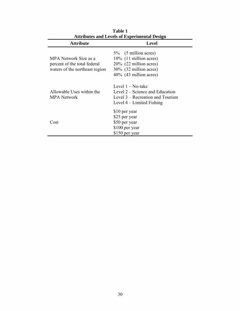
Table 1 Attributes and Levels of Experimental Design

Attribute Level

MPA Network Size as a percent of the total federal waters of the northeast region

5% (5 million acres) 10% (11 million acres) 20% (22 million acres) 30% (32 million acres) 40% (43 million acres)

Allowable Uses within the MPA Network

Level 1 – No-take Level 2 – Science and Education Level 3 – Recreation and Tourism Level 4 – Limited Fishing

Cost

$10 per year $25 per year $50 per year $100 per year $150 per year

30

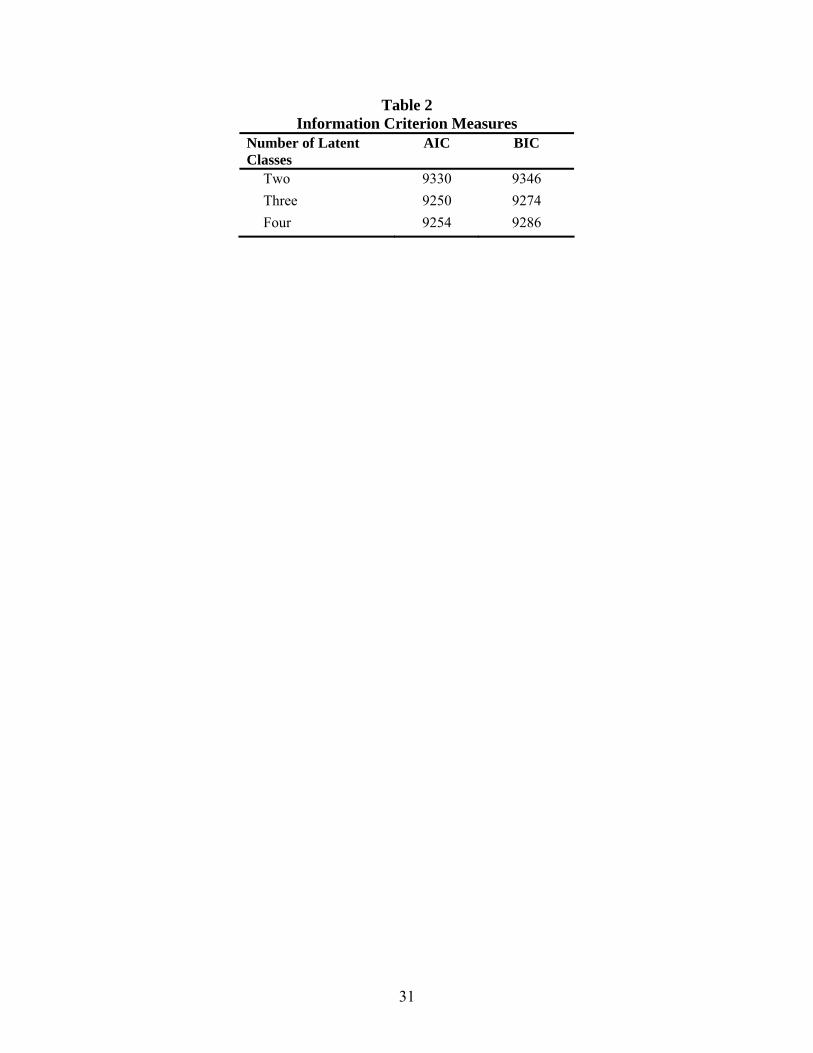
Table 2 Information Criterion Measures

Number of Latent Classes

AIC BIC

Two 9330 9346 Three 9250 9274 Four 9254 9286

31

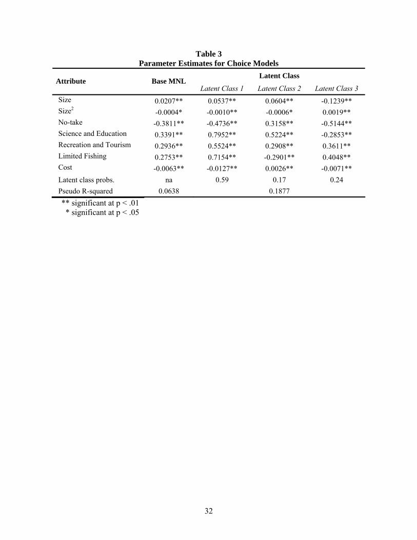
Table 3 Parameter Estimates for Choice Models

Latent Class Attribute Base MNL

Latent Class 1 Latent Class 2 Latent Class 3 Size 0.0207** 0.0537** 0.0604** -0.1239** Size2 -0.0004* -0.0010** -0.0006* 0.0019** No-take -0.3811** -0.4736** 0.3158** -0.5144** Science and Education 0.3391** 0.7952** 0.5224** -0.2853** Recreation and Tourism 0.2936** 0.5524** 0.2908** 0.3611** Limited Fishing 0.2753** 0.7154** -0.2901** 0.4048** Cost -0.0063** -0.0127** 0.0026** -0.0071** Latent class probs. na 0.59 0.17 0.24 Pseudo R-squared 0.0638 0.1877 ** significant at p < .01 * significant at p < .05

32

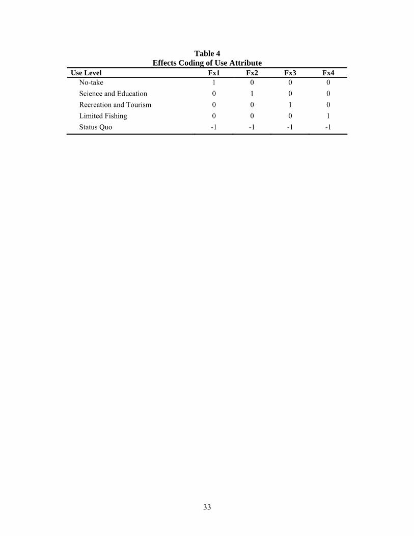
Table 4 Effects Coding of Use Attribute

Use Level Fx1 Fx2 Fx3 Fx4 No-take 1 0 0 0 Science and Education 0 1 0 0 Recreation and Tourism 0 0 1 0 Limited Fishing 0 0 0 1 Status Quo -1 -1 -1 -1

33

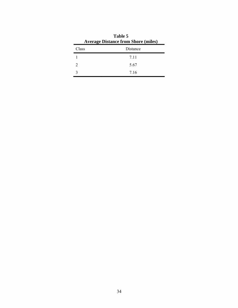
Table 5

Average Distance from Shore (miles) Class Distance

1 7.11

2 5.67

3 7.16

34

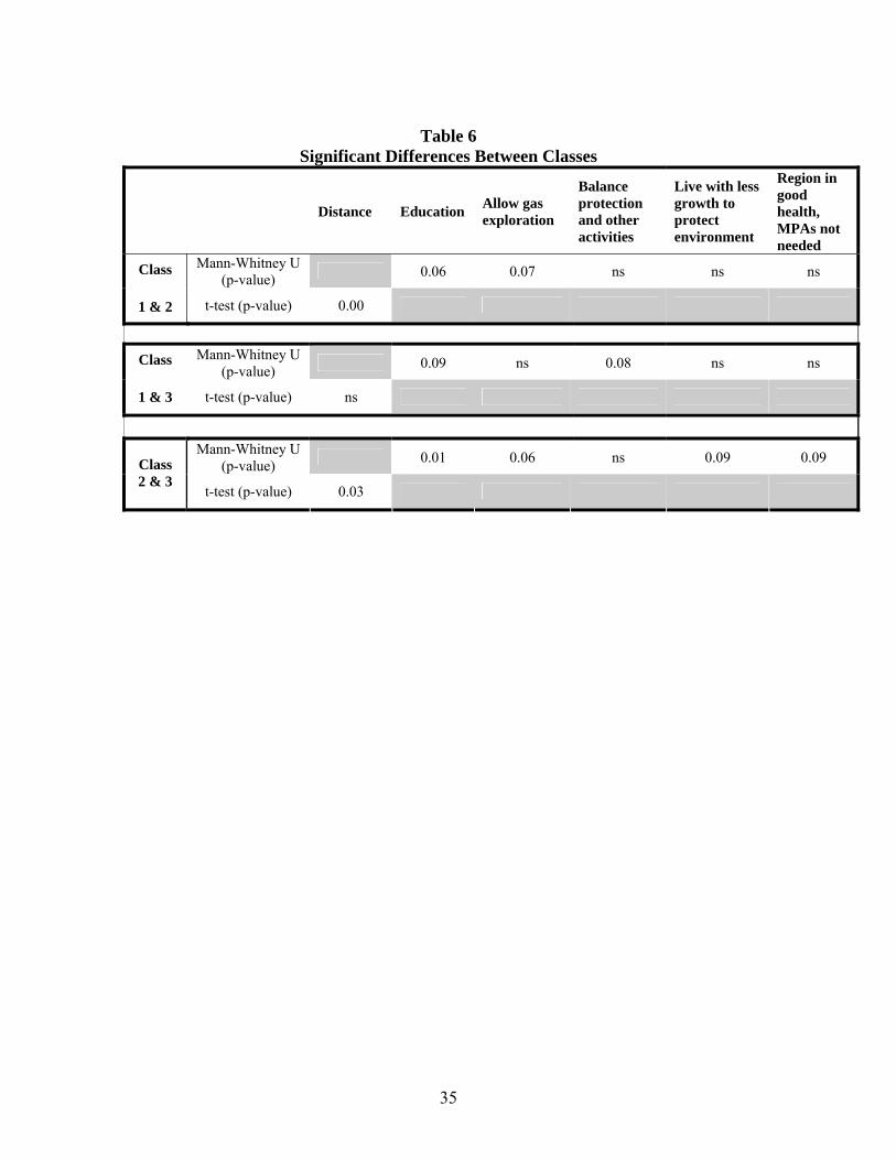
Table 6

Significant Differences Between Classes

Distance Education Allow gas exploration

Balance protection and other activities

Live with less growth to protect environment

Region in good health, MPAs not needed

Mann-Whitney U (p-value) 0.06 0.07 ns ns ns Class

1 & 2 t-test (p-value) 0.00

Mann-Whitney U

(p-value) 0.09 ns 0.08 ns ns Class

1 & 3 t-test (p-value) ns

Mann-Whitney U

(p-value) 0.01 0.06 ns 0.09 0.09 Class 2 & 3

t-test (p-value) 0.03

35

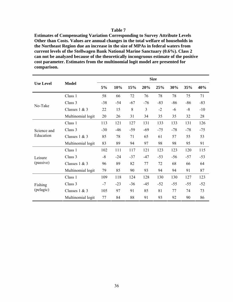
Table 7 Estimates of Compensating Variation Corresponding to Survey Attribute Levels Other than Costs. Values are annual changes in the total welfare of households in the Northeast Region due an increase in the size of MPAs in federal waters from current levels of the Stellwagen Bank National Marine Sanctuary (0.6%). Class 2 can not be analyzed because of the theoretically incongruous estimate of the positive cost parameter. Estimates from the multinomial logit model are presented for comparison.

Size

Use Level Model 5% 10% 15% 20% 25% 30% 35% 40%

Class 1 58 66 72 76 78 78 75 71 Class 3 -38 -54 -67 -76 -83 -86 -86 -83 Classes 1 & 3 22 15 8 3 -2 -6 -8 -10

No-Take

Multinomial logit 20 26 31 34 35 35 32 28 Class 1 113 121 127 131 133 133 131 126 Class 3 -30 -46 -59 -69 -75 -78 -78 -75 Classes 1 & 3 85 78 71 65 61 57 55 53

Science and Education

Multinomial logit 83 89 94 97 98 98 95 91 Class 1 102 111 117 121 123 123 120 115 Class 3 -8 -24 -37 -47 -53 -56 -57 -53 Classes 1 & 3 96 89 82 77 72 68 66 64

Leisure (passive)

Multinomial logit 79 85 90 93 94 94 91 87 Class 1 109 118 124 128 130 130 127 123 Class 3 -7 -23 -36 -45 -52 -55 -55 -52 Classes 1 & 3 105 97 91 85 81 77 74 73

Fishing (pelagic)

Multinomial logit 77 84 88 91 93 92 90 86

36

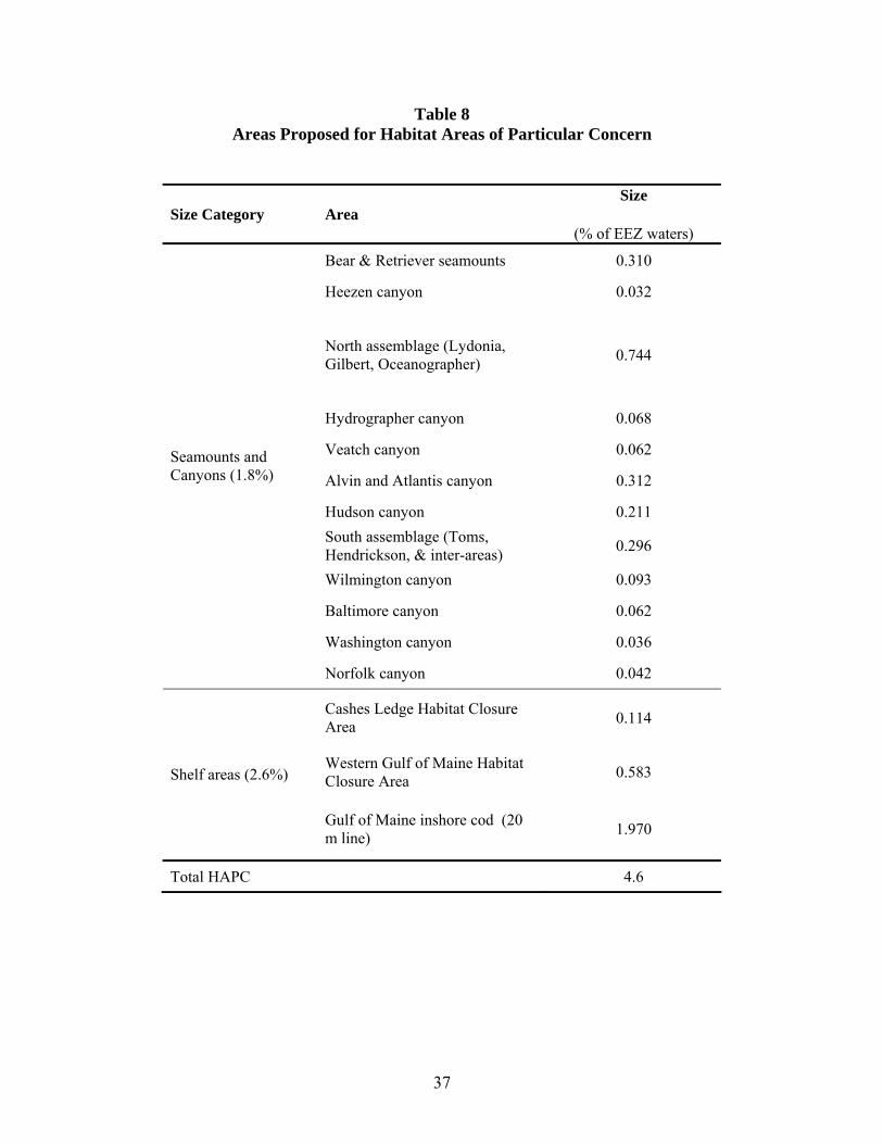
Table 8 Areas Proposed for Habitat Areas of Particular Concern

Size Category Area Size

(% of EEZ waters)

Bear & Retriever seamounts 0.310

Heezen canyon 0.032

North assemblage (Lydonia, Gilbert, Oceanographer)

0.744

Hydrographer canyon 0.068

Veatch canyon 0.062

Alvin and Atlantis canyon 0.312

Hudson canyon 0.211 South assemblage (Toms, Hendrickson, & inter-areas) 0.296

Wilmington canyon 0.093

Baltimore canyon 0.062

Washington canyon 0.036

Seamounts and Canyons (1.8%)

Norfolk canyon 0.042

Cashes Ledge Habitat Closure Area 0.114

Western Gulf of Maine Habitat Closure Area 0.583 Shelf areas (2.6%)

Gulf of Maine inshore cod (20 m line) 1.970

Total HAPC 4.6

37

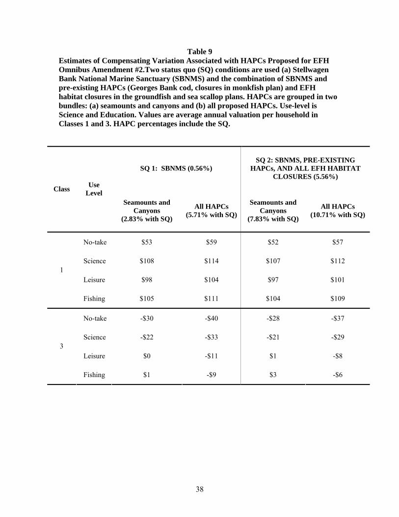
Table 9 Estimates of Compensating Variation Associated with HAPCs Proposed for EFH Omnibus Amendment #2.Two status quo (SQ) conditions are used (a) Stellwagen Bank National Marine Sanctuary (SBNMS) and the combination of SBNMS and pre-existing HAPCs (Georges Bank cod, closures in monkfish plan) and EFH habitat closures in the groundfish and sea scallop plans. HAPCs are grouped in two bundles: (a) seamounts and canyons and (b) all proposed HAPCs. Use-level is Science and Education. Values are average annual valuation per household in Classes 1 and 3. HAPC percentages include the SQ.

SQ 1: SBNMS (0.56%) SQ 2: SBNMS, PRE-EXISTING

HAPCs, AND ALL EFH HABITAT CLOSURES (5.56%)

Class Use Level

Seamounts and Canyons

(2.83% with SQ)

All HAPCs (5.71% with SQ)

Seamounts and Canyons

(7.83% with SQ)

All HAPCs (10.71% with SQ)

No-take $53 $59 $52 $57

Science $108 $114 $107 $112

Leisure $98 $104 $97 $101 1

Fishing $105 $111 $104 $109

No-take -$30 -$40 -$28 -$37

Science -$22 -$33 -$21 -$29

Leisure $0 -$11 $1 -$8 3

Fishing $1 -$9 $3 -$6

38

Figure 1 Sample Choice Task

Please compare the Alternatives below and choose the one Alternative you would most prefer for the Northeast Region. Alternative A Alternative B Current Situation

What is the combined Size of all of the MPA areas in the network?

2% (2 million acres)

2% (2 million acres)

What are the Allowable Uses within the MPA network?

Level 4 Limited Fishing

Level 2 Science and Education

What is the Cost to you each year if you voluntarily support an MPA network?

$25 $150

Click here to see the current

situation again <hyperlinked to

Section 5>

Which do you most prefer for the Federal Waters of the Northeast Region?

I prefer

Alternative A

I prefer

Alternative B

I prefer the

Current Situation

39

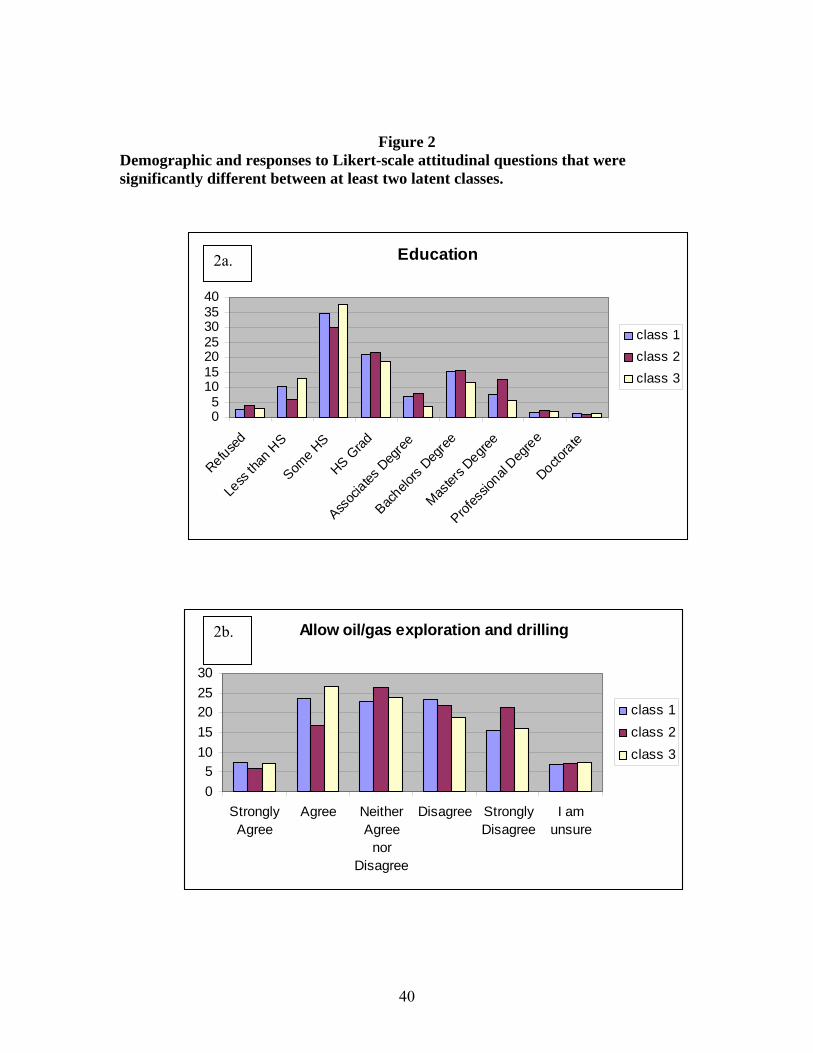
Figure 2 Demographic and responses to Likert-scale attitudinal questions that were significantly different between at least two latent classes.

Education

05

10152025303540

Refused

Less

than

HS

Some H

S

HS Grad

Assoc

iates D

egree

Bachelo

rs Deg

ree

Master

s Degre

e

Profes

sional

Degree

Doctorate

class 1class 2class 3

2a. Allow oil/gas exploration and drilling

05

1015202530

StronglyAgree

Agree NeitherAgree

norDisagree

Disagree StronglyDisagree

I amunsure

class 1class 2class 3

2b.

40

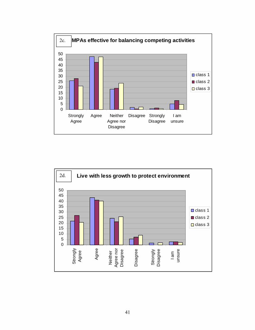
MPAs effective for balancing competing activities

05

101520253035404550

StronglyAgree

Agree NeitherAgree norDisagree

Disagree StronglyDisagree

I amunsure

class 1class 2class 3

2c.

Live with less growth to protect environment

05

101520253035404550

Stro

ngly

Agre

e

Agr

ee

Nei

ther

Agr

ee n

orD

isag

ree

Dis

agre

e

Stro

ngly

Dis

agre

e

I am

unsu

re

class 1

class 2class 3

2d.

41

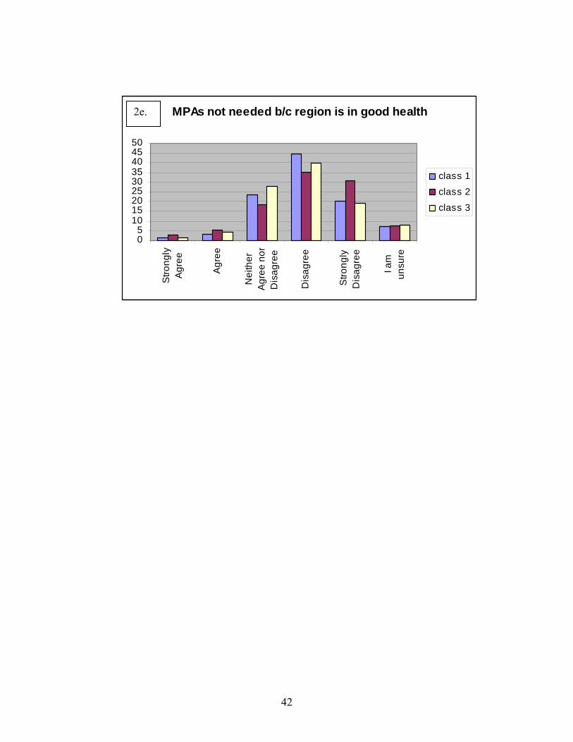
MPAs not needed b/c region is in good health

05

101520253035404550

Stro

ngly

Agre

e

Agr

ee

Nei

ther

Agr

ee n

orD

isag

ree

Dis

agre

e

Stro

ngly

Dis

agre

e

I am

unsu

re

class 1class 2

class 3

2e.

42

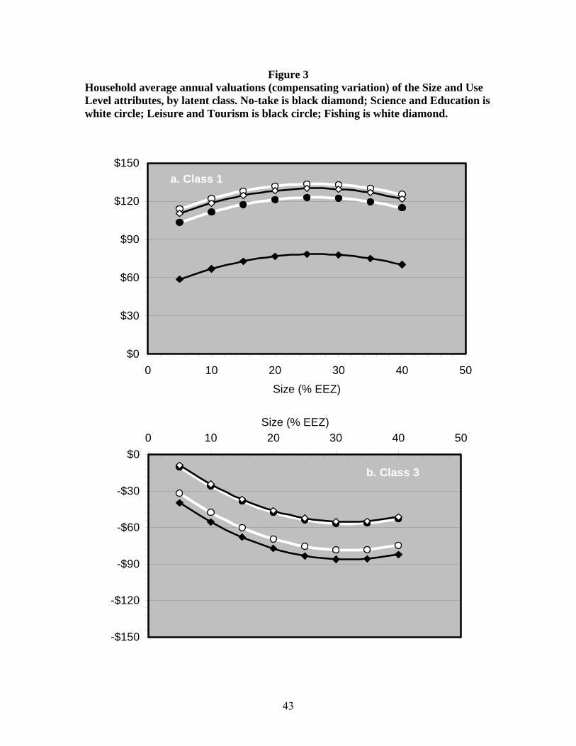
Figure 3 Household average annual valuations (compensating variation) of the Size and Use Level attributes, by latent class. No-take is black diamond; Science and Education is white circle; Leisure and Tourism is black circle; Fishing is white diamond.

a. Class 1

$0

$30

$60

$90

$120

$150

0 10 20 30 40 5

Size (% EEZ)

0

b. Class 3

-$150

-$120

-$90

-$60

-$30

$00 10 20 30 40 50

Size (% EEZ)

43

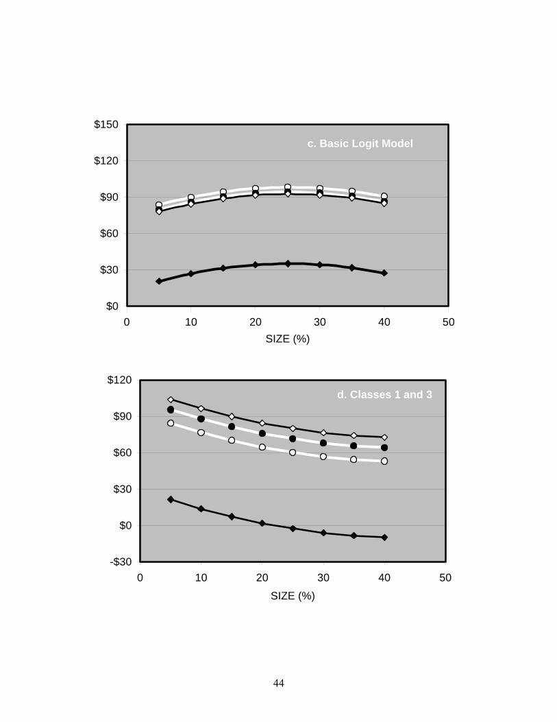
c. Basic Logit Model

$0

$30

$60

$90

$120

$150

0 10 20 30 40 5SIZE (%)

0

d. Classes 1 and 3

-$30

$0

$30

$60

$90

$120

0 10 20 30 40 50

SIZE (%)

44

Figure 4 Marginal Value of Size and Optimal Allocation when Costs are Zero

-$2

-$1

$0

$1

$2

0 10 20 30 40 5

Size (% of EEZ)

0

Class 1 (positive utility)

Class 3 (disutility)

Basic logit

27%26%

45

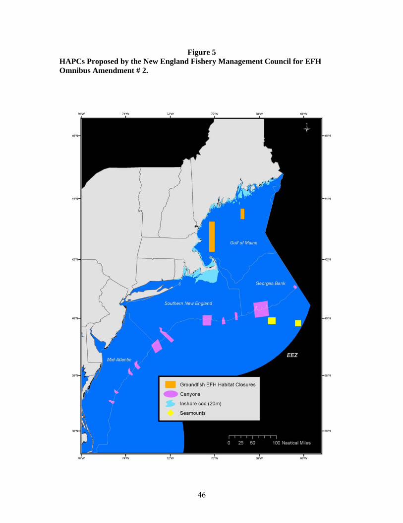
Figure 5 HAPCs Proposed by the New England Fishery Management Council for EFH Omnibus Amendment # 2.

46

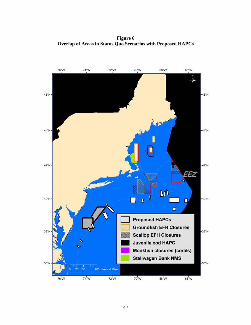
Figure 6

Overlap of Areas in Status Quo Scenarios with Proposed HAPCs

47

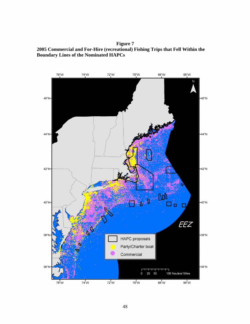
Figure 7 2005 Commercial and For-Hire (recreational) Fishing Trips that Fell Within the Boundary Lines of the Nominated HAPCs

48

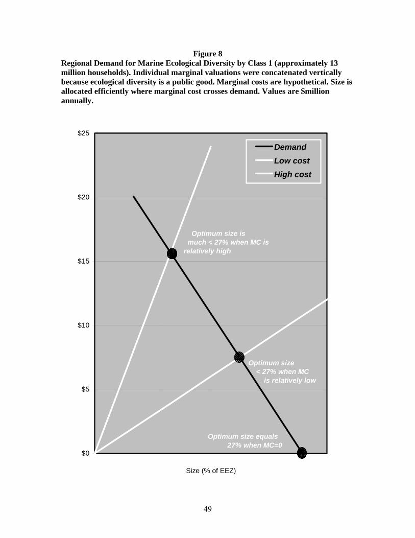
Figure 8 Regional Demand for Marine Ecological Diversity by Class 1 (approximately 13 million households). Individual marginal valuations were concatenated vertically because ecological diversity is a public good. Marginal costs are hypothetical. Size is allocated efficiently where marginal cost crosses demand. Values are $million annually.

$0

$5

$10

$15

$20

$25

0 5 10 15 20 25 30

Size (% of EEZ)

DemandLow costHigh cost

Optimum size equals 27% when MC=0

Optimum size < 27% when MC is relatively low

Optimum size is much < 27% when MC is relatively high

49

Appendices to:

“Estimating Non-market Values for Marine Protected Areas: A Latent Class Modeling Approach”

Appendix A: The web-based questionnaire

Appendix B: Sampling and self-selection biases Appendix C: Responses to attitudinal and opinion questions

50

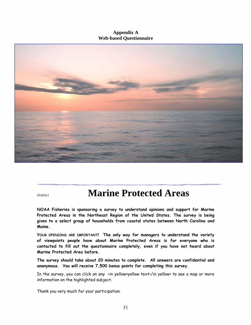
Appendix A Web-based Questionnaire

Marine Protected Areas [display]

NOAA Fisheries is sponsoring a survey to understand opinions and support for Marine Protected Areas in the Northeast Region of the United States. The survey is being given to a select group of households from coastal states between North Carolina and Maine.

YOUR OPINIONS ARE IMPORTANT! The only way for managers to understand the variety of viewpoints people have about Marine Protected Areas is for everyone who is contacted to fill out the questionnaire completely, even if you have not heard about Marine Protected Area before.

The survey should take about 20 minutes to complete. All answers are confidential and anonymous. You will receive 7,500 bonus points for completing this survey.

In the survey, you can click on any <in yellow>yellow text</in yellow> to see a map or more information on the highlighted subject. Thank you very much for your participation.

51

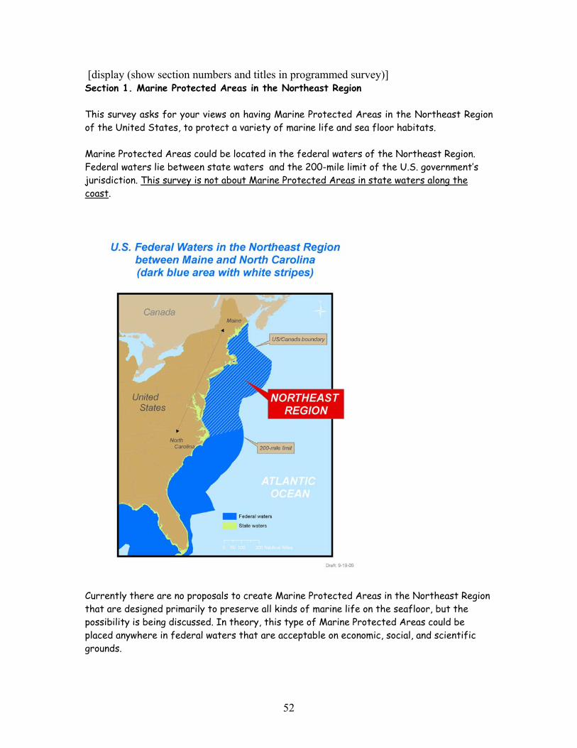
[display (show section numbers and titles in programmed survey)] Section 1. Marine Protected Areas in the Northeast Region This survey asks for your views on having Marine Protected Areas in the Northeast Region of the United States, to protect a variety of marine life and sea floor habitats. Marine Protected Areas could be located in the federal waters of the Northeast Region. Federal waters lie between state waters and the 200-mile limit of the U.S. government’s jurisdiction. This survey is not about Marine Protected Areas in state waters along the coast.

Currently there are no proposals to create Marine Protected Areas in the Northeast Region that are designed primarily to preserve all kinds of marine life on the seafloor, but the possibility is being discussed. In theory, this type of Marine Protected Areas could be placed anywhere in federal waters that are acceptable on economic, social, and scientific grounds.

52

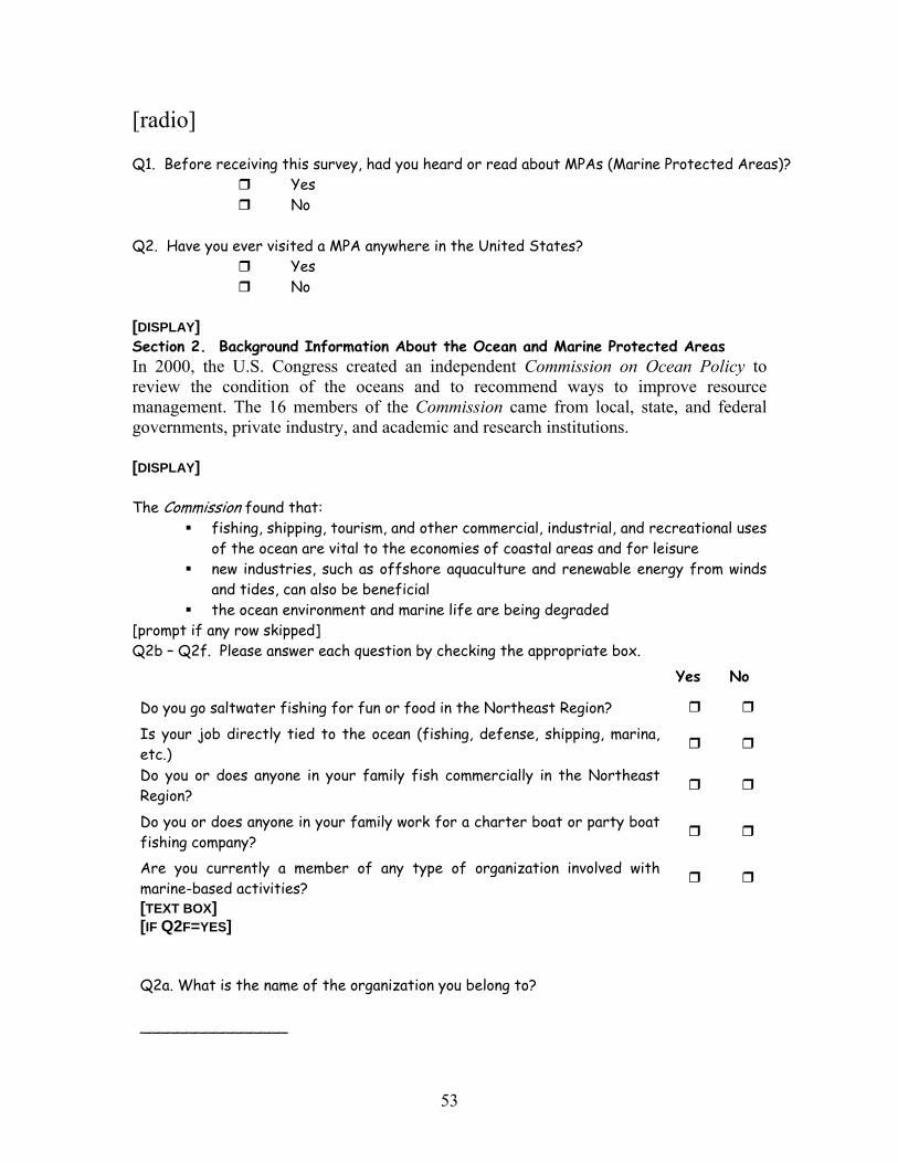
[radio] Q1. Before receiving this survey, had you heard or read about MPAs (Marine Protected Areas)? Yes No Q2. Have you ever visited a MPA anywhere in the United States? Yes No [DISPLAY] Section 2. Background Information About the Ocean and Marine Protected Areas In 2000, the U.S. Congress created an independent Commission on Ocean Policy to review the condition of the oceans and to recommend ways to improve resource management. The 16 members of the Commission came from local, state, and federal governments, private industry, and academic and research institutions. [DISPLAY] The Commission found that:

fishing, shipping, tourism, and other commercial, industrial, and recreational uses of the ocean are vital to the economies of coastal areas and for leisure

new industries, such as offshore aquaculture and renewable energy from winds and tides, can also be beneficial

the ocean environment and marine life are being degraded [prompt if any row skipped] Q2b – Q2f. Please answer each question by checking the appropriate box. Yes No

Do you go saltwater fishing for fun or food in the Northeast Region?

Is your job directly tied to the ocean (fishing, defense, shipping, marina, etc.)

Do you or does anyone in your family fish commercially in the Northeast Region?

Do you or does anyone in your family work for a charter boat or party boat fishing company?

Are you currently a member of any type of organization involved with marine-based activities?

[TEXT BOX] [IF Q2F=YES] Q2a. What is the name of the organization you belong to? ________________

53

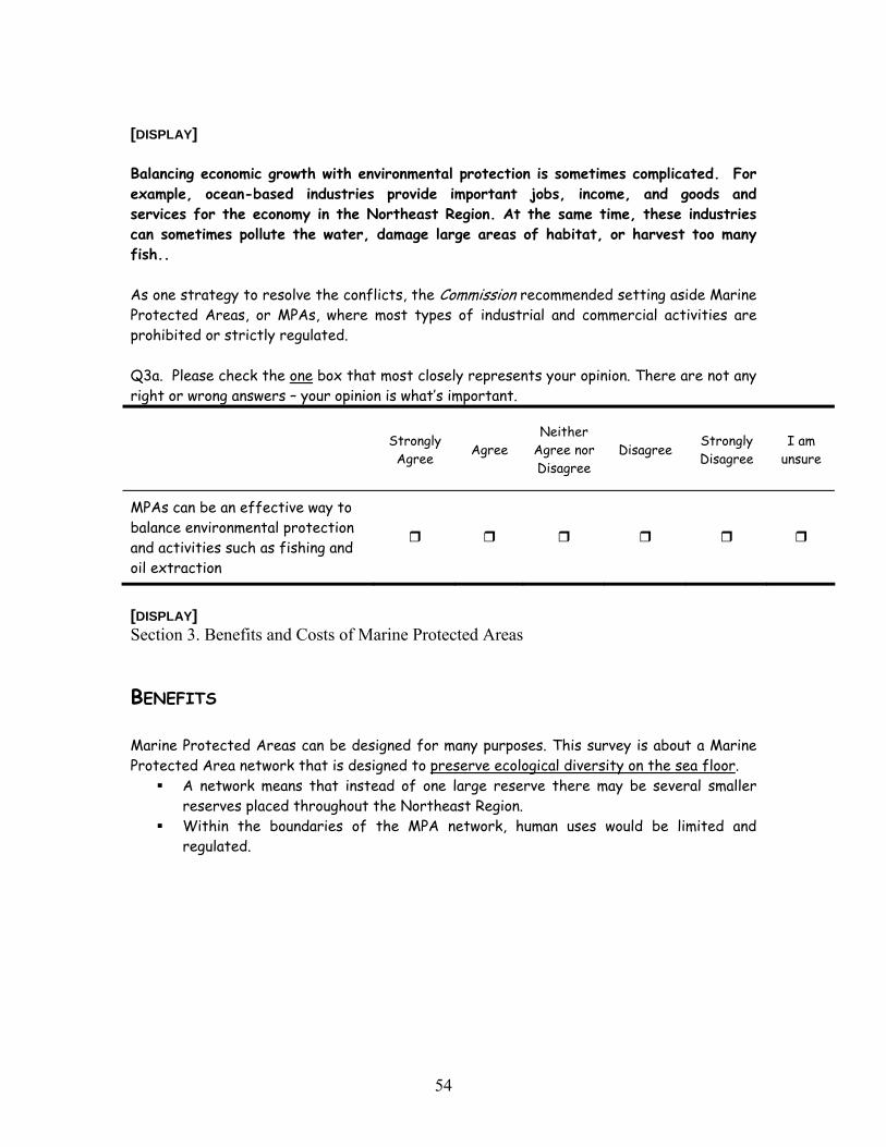
[DISPLAY] Balancing economic growth with environmental protection is sometimes complicated. For example, ocean-based industries provide important jobs, income, and goods and services for the economy in the Northeast Region. At the same time, these industries can sometimes pollute the water, damage large areas of habitat, or harvest too many fish.. As one strategy to resolve the conflicts, the Commission recommended setting aside Marine Protected Areas, or MPAs, where most types of industrial and commercial activities are prohibited or strictly regulated. Q3a. Please check the one box that most closely represents your opinion. There are not any right or wrong answers – your opinion is what’s important.

Strongly Agree Agree

Neither Agree nor Disagree

Disagree Strongly Disagree

I am unsure

MPAs can be an effective way to balance environmental protection and activities such as fishing and oil extraction

[DISPLAY] Section 3. Benefits and Costs of Marine Protected Areas

BENEFITS Marine Protected Areas can be designed for many purposes. This survey is about a Marine Protected Area network that is designed to preserve ecological diversity on the sea floor.

A network means that instead of one large reserve there may be several smaller reserves placed throughout the Northeast Region.

Within the boundaries of the MPA network, human uses would be limited and regulated.

54

[display] The primary benefits of the Marine Protected Area network are:

Preservation of the variety of marine life in the Northeast Region (fish, shellfish, plants) in their natural habitats on the bottom of the ocean - regardless of their commercial or recreational importance.

Preventing future industrial uses within the MPA network boundaries.

There might also be incidental benefits associated with the MPA network, but these are uncertain. Incidental benefits might include increased catches by fisheries outside of the boundaries of the MPA network, a temporary sanctuary for animals that migrate into and out of the region (such as herring and tuna), and possible medical or pharmaceutical discoveries from species that were preserved. [GRID] [SHOW HEADER ON TOP AND BOTTOM OF SCREEN] Q3. For each statement below, please check the one box that most closely represents your opinion. There are not any right or wrong answers – your opinion is what’s important.

Strongly Agree Agree

Neither Agree nor Disagree

Disagree Strongly Disagree

I am unsure

MPAs are not needed in the Northeast Region because marine life and ocean habitats are in good shape

I like knowing that part of the ocean in the Northeast Region is protected even if I never see or use it

MPAs should not be established unless their rules and boundaries can be completely enforced

55

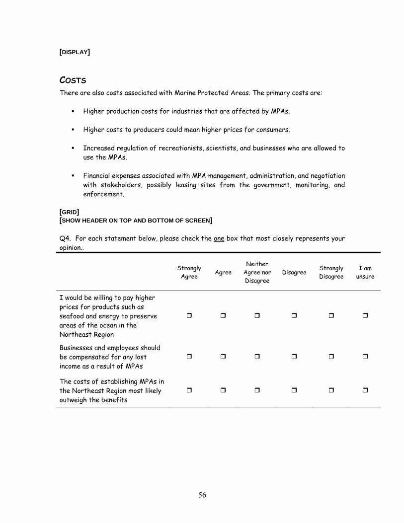
[DISPLAY]

COSTS There are also costs associated with Marine Protected Areas. The primary costs are:

Higher production costs for industries that are affected by MPAs. Higher costs to producers could mean higher prices for consumers.

Increased regulation of recreationists, scientists, and businesses who are allowed to

use the MPAs. Financial expenses associated with MPA management, administration, and negotiation

with stakeholders, possibly leasing sites from the government, monitoring, and enforcement.

[GRID] [SHOW HEADER ON TOP AND BOTTOM OF SCREEN] Q4. For each statement below, please check the one box that most closely represents your opinion..

Strongly Agree Agree

Neither Agree nor Disagree

Disagree Strongly Disagree

I am unsure

I would be willing to pay higher prices for products such as seafood and energy to preserve areas of the ocean in the Northeast Region

Businesses and employees should be compensated for any lost income as a result of MPAs

The costs of establishing MPAs in the Northeast Region most likely outweigh the benefits

56

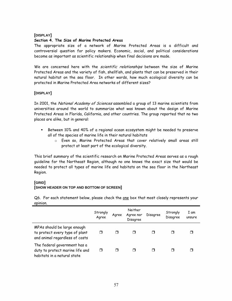
[DISPLAY] Section 4. The Size of Marine Protected Areas The appropriate size of a network of Marine Protected Areas is a difficult and controversial question for policy makers. Economic, social, and political considerations become as important as scientific relationship when final decisions are made. We are concerned here with the scientific relationships between the size of Marine Protected Areas and the variety of fish, shellfish, and plants that can be preserved in their natural habitat on the sea floor. In other words, how much ecological diversity can be protected in Marine Protected Area networks of different sizes? [DISPLAY] In 2001, the National Academy of Sciences assembled a group of 13 marine scientists from universities around the world to summarize what was known about the design of Marine Protected Areas in Florida, California, and other countries. The group reported that no two places are alike, but in general:

Between 10% and 40% of a regional ocean ecosystem might be needed to preserve all of the species of marine life in their natural habitats

o Even so, Marine Protected Areas that cover relatively small areas still protect at least part of the ecological diversity.

This brief summary of the scientific research on Marine Protected Areas serves as a rough guideline for the Northeast Region, although no one knows the exact size that would be needed to protect all types of marine life and habitats on the sea floor in the Northeast Region. [GRID] [SHOW HEADER ON TOP AND BOTTOM OF SCREEN] Q6. For each statement below, please check the one box that most closely represents your opinion.

Strongly Agree Agree

Neither Agree nor Disagree

Disagree Strongly Disagree

I am unsure

MPAs should be large enough to protect every type of plant and animal regardless of costs

The federal government has a duty to protect marine life and habitats in a natural state

57

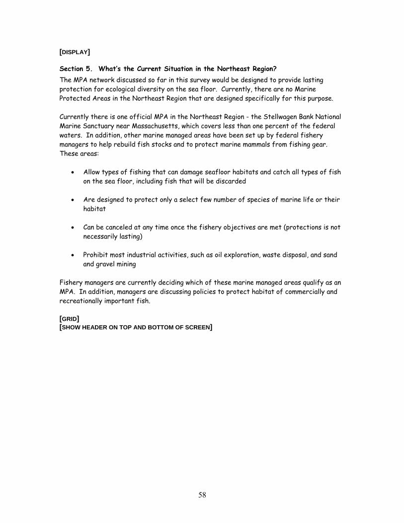
[DISPLAY]

Section 5. What’s the Current Situation in the Northeast Region? The MPA network discussed so far in this survey would be designed to provide lasting protection for ecological diversity on the sea floor. Currently, there are no Marine Protected Areas in the Northeast Region that are designed specifically for this purpose. Currently there is one official MPA in the Northeast Region - the Stellwagen Bank National Marine Sanctuary near Massachusetts, which covers less than one percent of the federal waters. In addition, other marine managed areas have been set up by federal fishery managers to help rebuild fish stocks and to protect marine mammals from fishing gear. These areas:

• Allow types of fishing that can damage seafloor habitats and catch all types of fish on the sea floor, including fish that will be discarded

• Are designed to protect only a select few number of species of marine life or their

habitat • Can be canceled at any time once the fishery objectives are met (protections is not

necessarily lasting) • Prohibit most industrial activities, such as oil exploration, waste disposal, and sand

and gravel mining

Fishery managers are currently deciding which of these marine managed areas qualify as an MPA. In addition, managers are discussing policies to protect habitat of commercially and recreationally important fish. [GRID] [SHOW HEADER ON TOP AND BOTTOM OF SCREEN]

58

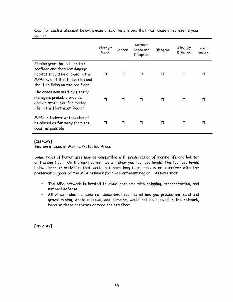
Q5. For each statement below, please check the one box that most closely represents your opinion.

Strongly Agree Agree

Neither Agree nor Disagree

Disagree Strongly Disagree

I am unsure

Fishing gear that sits on the seafloor and does not damage habitat should be allowed in the MPAs even if it catches fish and shellfish living on the sea floor

The areas now used by fishery managers probably provide enough protection for marine life in the Northeast Region

MPAs in federal waters should be placed as far away from the coast as possible

[DISPLAY] Section 6. Uses of Marine Protected Areas

Some types of human uses may be compatible with preservation of marine life and habitat on the sea floor. On the next screen, we will show you four use levels. The four use levels below describe activities that would not have long-term impacts or interfere with the preservation goals of the MPA network for the Northeast Region. Assume that:

The MPA network is located to avoid problems with shipping, transportation, and national defense.

All other industrial uses not described, such as oil and gas production, sand and gravel mining, waste disposal, and dumping, would not be allowed in the network, because these activities damage the sea floor.

[DISPLAY]

59

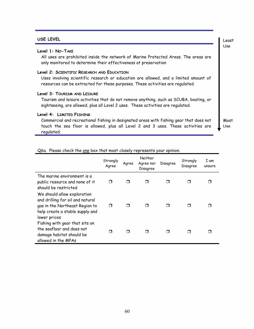
USE LEVEL

Level 1: NO-TAKE All uses are prohibited inside the network of Marine Protected Areas. The areas are only monitored to determine their effectiveness at preservation

Level 2: SCIENTIFIC RESEARCH AND EDUCATION Uses involving scientific research or education are allowed, and a limited amount of resources can be extracted for these purposes. These activities are regulated.

Level 3: TOURISM AND LEISURE Tourism and leisure activities that do not remove anything, such as SCUBA, boating, or sightseeing, are allowed, plus all Level 2 uses. These activities are regulated.

Level 4: LIMITED FISHING Commercial and recreational fishing in designated areas with fishing gear that does not touch the sea floor is allowed, plus all Level 2 and 3 uses. These activities are regulated.

Most Use

Least Use

Q6a. Please check the one box that most closely represents your opinion.

Strongly Agree Agree

Neither Agree nor Disagree

Disagree Strongly Disagree

I am unsure

The marine environment is a public resource and none of it should be restricted

We should allow exploration and drilling for oil and natural gas in the Northeast Region to help create a stable supply and lower prices

Fishing with gear that sits on the seafloor and does not damage habitat should be allowed in the MPAs

60

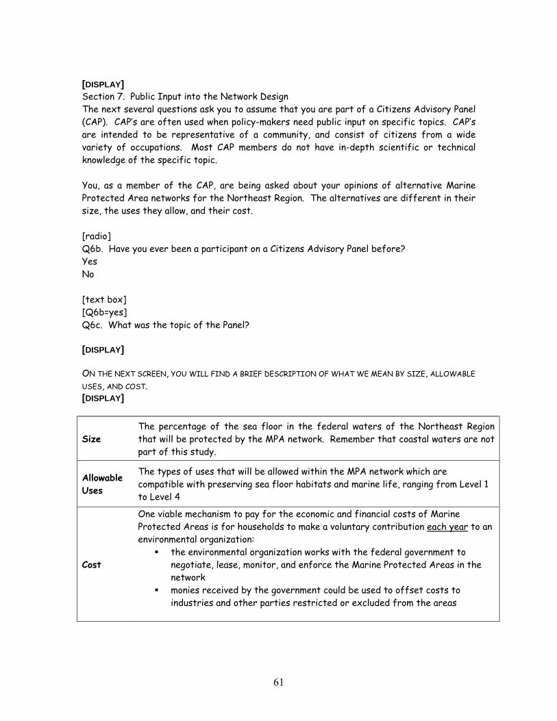
[DISPLAY] Section 7. Public Input into the Network Design The next several questions ask you to assume that you are part of a Citizens Advisory Panel (CAP). CAP’s are often used when policy-makers need public input on specific topics. CAP’s are intended to be representative of a community, and consist of citizens from a wide variety of occupations. Most CAP members do not have in-depth scientific or technical knowledge of the specific topic.

You, as a member of the CAP, are being asked about your opinions of alternative Marine Protected Area networks for the Northeast Region. The alternatives are different in their size, the uses they allow, and their cost. [radio] Q6b. Have you ever been a participant on a Citizens Advisory Panel before? Yes No [text box] [Q6b=yes] Q6c. What was the topic of the Panel? [DISPLAY] ON THE NEXT SCREEN, YOU WILL FIND A BRIEF DESCRIPTION OF WHAT WE MEAN BY SIZE, ALLOWABLE USES, AND COST. [DISPLAY]

Size The percentage of the sea floor in the federal waters of the Northeast Region that will be protected by the MPA network. Remember that coastal waters are not part of this study.

Allowable Uses

The types of uses that will be allowed within the MPA network which are compatible with preserving sea floor habitats and marine life, ranging from Level 1 to Level 4

Cost

One viable mechanism to pay for the economic and financial costs of Marine Protected Areas is for households to make a voluntary contribution each year to an environmental organization:

the environmental organization works with the federal government to negotiate, lease, monitor, and enforce the Marine Protected Areas in the network

monies received by the government could be used to offset costs to industries and other parties restricted or excluded from the areas

61

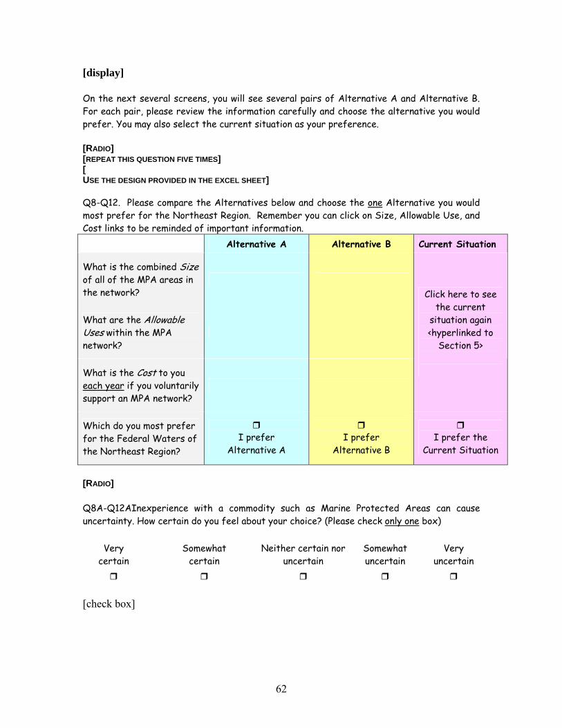
[display] On the next several screens, you will see several pairs of Alternative A and Alternative B. For each pair, please review the information carefully and choose the alternative you would prefer. You may also select the current situation as your preference. [RADIO] [REPEAT THIS QUESTION FIVE TIMES] [ USE THE DESIGN PROVIDED IN THE EXCEL SHEET] Q8-Q12. Please compare the Alternatives below and choose the one Alternative you would most prefer for the Northeast Region. Remember you can click on Size, Allowable Use, and Cost links to be reminded of important information. Alternative A Alternative B Current Situation

What is the combined Size of all of the MPA areas in the network?

What are the Allowable Uses within the MPA network?

What is the Cost to you each year if you voluntarily support an MPA network?

Click here to see the current

situation again <hyperlinked to

Section 5>

Which do you most prefer for the Federal Waters of the Northeast Region?

I prefer

Alternative A

I prefer

Alternative B

I prefer the

Current Situation

[RADIO] Q8A-Q12AInexperience with a commodity such as Marine Protected Areas can cause uncertainty. How certain do you feel about your choice? (Please check only one box)

Very certain

Somewhat certain

Neither certain nor uncertain

Somewhat uncertain

Very uncertain

[check box]

62

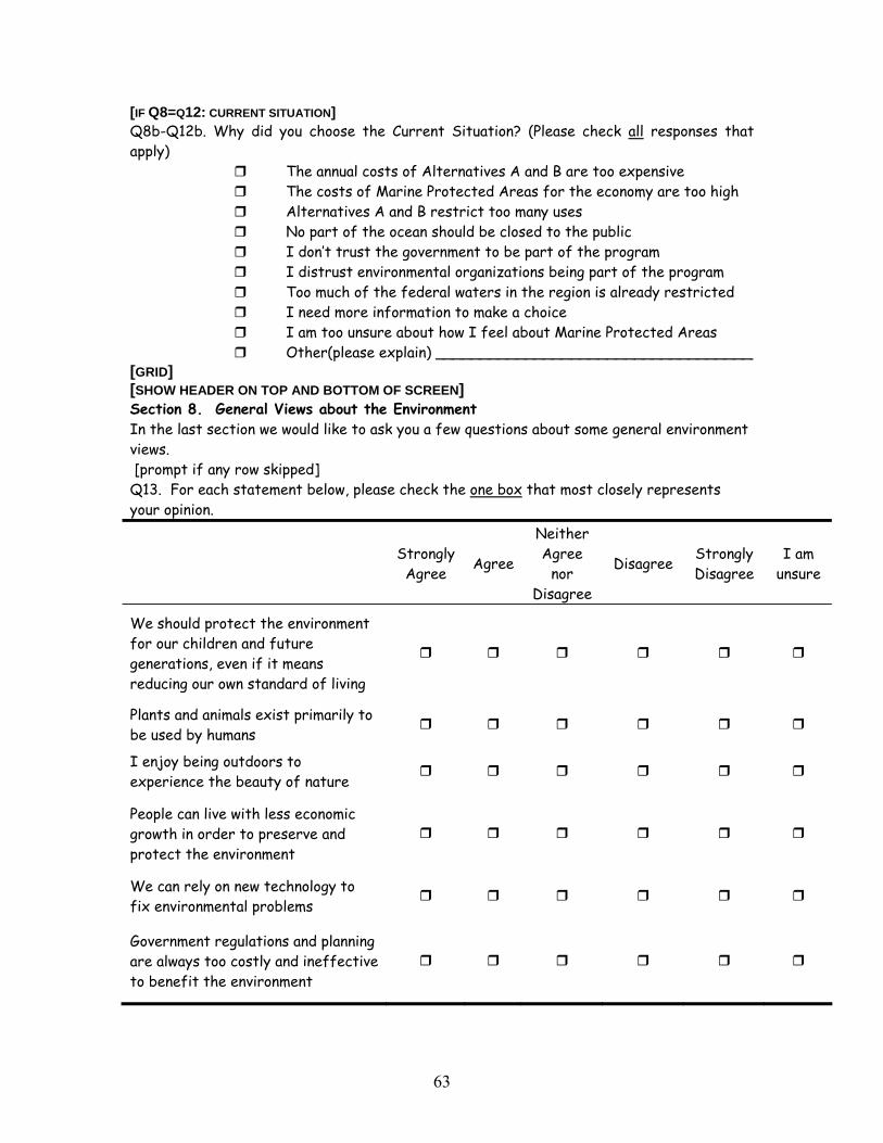
[IF Q8=Q12: CURRENT SITUATION] Q8b-Q12b. Why did you choose the Current Situation? (Please check all responses that apply)

The annual costs of Alternatives A and B are too expensive The costs of Marine Protected Areas for the economy are too high Alternatives A and B restrict too many uses No part of the ocean should be closed to the public I don’t trust the government to be part of the program I distrust environmental organizations being part of the program Too much of the federal waters in the region is already restricted I need more information to make a choice I am too unsure about how I feel about Marine Protected Areas Other(please explain) ___________________________________

[GRID] [SHOW HEADER ON TOP AND BOTTOM OF SCREEN] Section 8. General Views about the Environment In the last section we would like to ask you a few questions about some general environment views. [prompt if any row skipped] Q13. For each statement below, please check the one box that most closely represents your opinion.

Strongly Agree Agree

Neither Agree

nor Disagree

Disagree Strongly Disagree

I am unsure

We should protect the environment for our children and future generations, even if it means reducing our own standard of living

Plants and animals exist primarily to be used by humans

I enjoy being outdoors to experience the beauty of nature

People can live with less economic growth in order to preserve and protect the environment

We can rely on new technology to fix environmental problems

Government regulations and planning are always too costly and ineffective to benefit the environment

63

64

[RADIO] Q14. How familiar were you with Marine Protected Areas before taking this survey?

Very familiar Somewhat familiar Unfamiliar [RADIO] Q15. How familiar are you now with Marine Protected Areas?

Very familiar Somewhat familiar Unfamiliar [TEXT BOX] Thank you for taking the time to complete this survey. Please provide any additional comments you have about the survey in the box below.

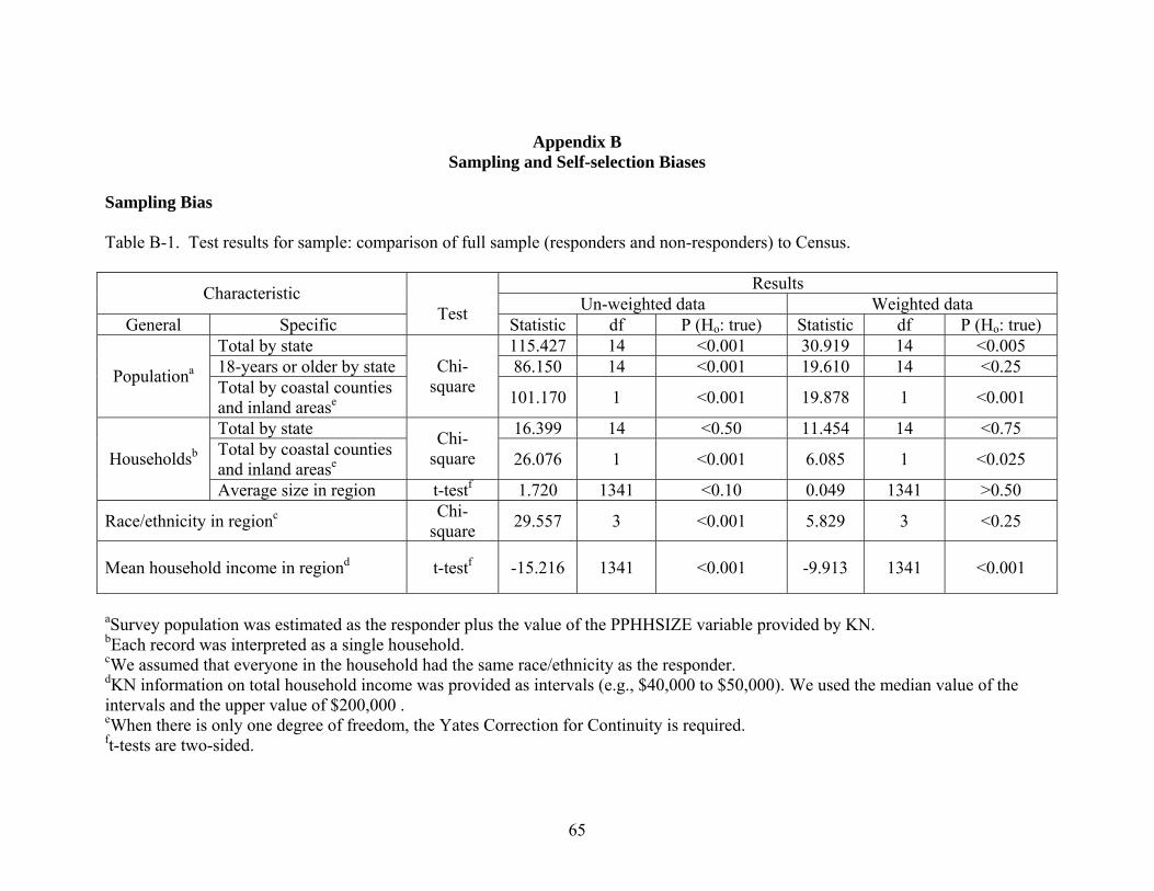
Appendix B Sampling and Self-selection Biases

Sampling Bias Table B-1. Test results for sample: comparison of full sample (responders and non-responders) to Census.

Results Characteristic Un-weighted data Weighted data General Specific

Test Statistic df P (Ho: true) Statistic df P (Ho: true)

Total by state 115.427 14 <0.001 30.919 14 <0.005 18-years or older by state 86.150 14 <0.001 19.610 14 <0.25 Populationa

Total by coastal counties and inland arease

Chi-square 101.170 1 <0.001 19.878 1 <0.001

Total by state 16.399 14 <0.50 11.454 14 <0.75 Total by coastal counties and inland arease

Chi-square 26.076 1 <0.001 6.085 1 <0.025 Householdsb

Average size in region t-testf 1.720 1341 <0.10 0.049 1341 >0.50

Race/ethnicity in regionc Chi-square 29.557 3 <0.001 5.829 3 <0.25

Mean household income in regiond t-testf -15.216 1341 <0.001 -9.913 1341 <0.001

aSurvey population was estimated as the responder plus the value of the PPHHSIZE variable provided by KN. bEach record was interpreted as a single household. cWe assumed that everyone in the household had the same race/ethnicity as the responder. dKN information on total household income was provided as intervals (e.g., $40,000 to $50,000). We used the median value of the intervals and the upper value of $200,000 . eWhen there is only one degree of freedom, the Yates Correction for Continuity is required. ft-tests are two-sided.

65

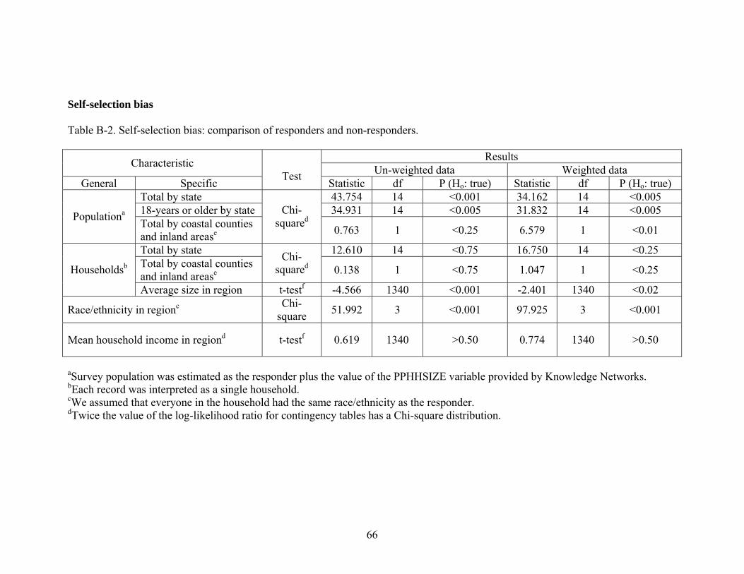
66

Self-selection bias Table B-2. Self-selection bias: comparison of responders and non-responders.

Results Characteristic Un-weighted data Weighted data General Specific

Test Statistic df P (Ho: true) Statistic df P (Ho: true)

Total by state 43.754 14 <0.001 34.162 14 <0.005 18-years or older by state 34.931 14 <0.005 31.832 14 <0.005 Populationa

Total by coastal counties and inland arease

Chi-squared

0.763 1 <0.25 6.579 1 <0.01

Total by state 12.610 14 <0.75 16.750 14 <0.25 Total by coastal counties and inland arease

Chi-squared 0.138 1 <0.75 1.047 1 <0.25 Householdsb

Average size in region t-testf -4.566 1340 <0.001 -2.401 1340 <0.02

Race/ethnicity in regionc Chi-square 51.992 3 <0.001 97.925 3 <0.001

Mean household income in regiond t-testf 0.619 1340 >0.50 0.774 1340 >0.50

aSurvey population was estimated as the responder plus the value of the PPHHSIZE variable provided by Knowledge Networks. bEach record was interpreted as a single household. cWe assumed that everyone in the household had the same race/ethnicity as the responder. dTwice the value of the log-likelihood ratio for contingency tables has a Chi-square distribution.

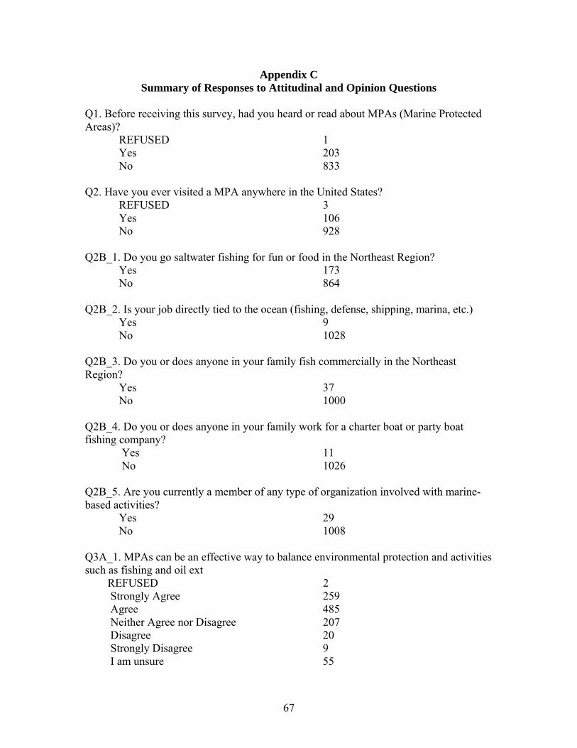
Appendix C Summary of Responses to Attitudinal and Opinion Questions

Q1. Before receiving this survey, had you heard or read about MPAs (Marine Protected Areas)? REFUSED 1 Yes 203 No 833 Q2. Have you ever visited a MPA anywhere in the United States? REFUSED 3 Yes 106 No 928 Q2B_1. Do you go saltwater fishing for fun or food in the Northeast Region? Yes 173 No 864 Q2B_2. Is your job directly tied to the ocean (fishing, defense, shipping, marina, etc.) Yes 9 No 1028 Q2B_3. Do you or does anyone in your family fish commercially in the Northeast Region? Yes 37 No 1000 Q2B_4. Do you or does anyone in your family work for a charter boat or party boat fishing company? Yes 11 No 1026 Q2B_5. Are you currently a member of any type of organization involved with marine-based activities? Yes 29 No 1008 Q3A_1. MPAs can be an effective way to balance environmental protection and activities such as fishing and oil ext REFUSED 2 Strongly Agree 259 Agree 485 Neither Agree nor Disagree 207 Disagree 20 Strongly Disagree 9 I am unsure 55

67

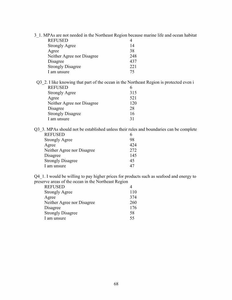
3_1. MPAs are not needed in the Northeast Region because marine life and ocean habitat REFUSED 4 Strongly Agree 14 Agree 38 Neither Agree nor Disagree 248 Disagree 437 Strongly Disagree 221 I am unsure 75 Q3_2. I like knowing that part of the ocean in the Northeast Region is protected even i REFUSED 6 Strongly Agree 315 Agree 521 Neither Agree nor Disagree 120 Disagree 28 Strongly Disagree 16 I am unsure 31 Q3_3. MPAs should not be established unless their rules and boundaries can be complete REFUSED 6 Strongly Agree 98 Agree 424 Neither Agree nor Disagree 272 Disagree 145 Strongly Disagree 45 I am unsure 47 Q4_1. I would be willing to pay higher prices for products such as seafood and energy to preserve areas of the ocean in the Northeast Region REFUSED 4 Strongly Agree 110 Agree 374 Neither Agree nor Disagree 260 Disagree 176 Strongly Disagree 58 I am unsure 55

68

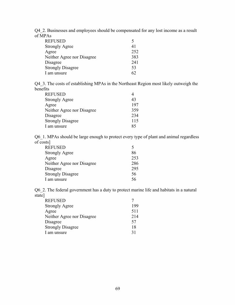
Q4_2. Businesses and employees should be compensated for any lost income as a result of MPAs REFUSED 5 Strongly Agree 41 Agree 252 Neither Agree nor Disagree 383 Disagree 241 Strongly Disagree 53 I am unsure 62 Q4_3. The costs of establishing MPAs in the Northeast Region most likely outweigh the benefits REFUSED 4 Strongly Agree 43 Agree 197 Neither Agree nor Disagree 359 Disagree 234 Strongly Disagree 115 I am unsure 85 Q6_1. MPAs should be large enough to protect every type of plant and animal regardless of costs] REFUSED 5 Strongly Agree 86 Agree 253 Neither Agree nor Disagree 286 Disagree 295 Strongly Disagree 56 I am unsure 56 Q6_2. The federal government has a duty to protect marine life and habitats in a natural state] REFUSED 7 Strongly Agree 199 Agree 511 Neither Agree nor Disagree 214 Disagree 57 Strongly Disagree 18 I am unsure 31

69

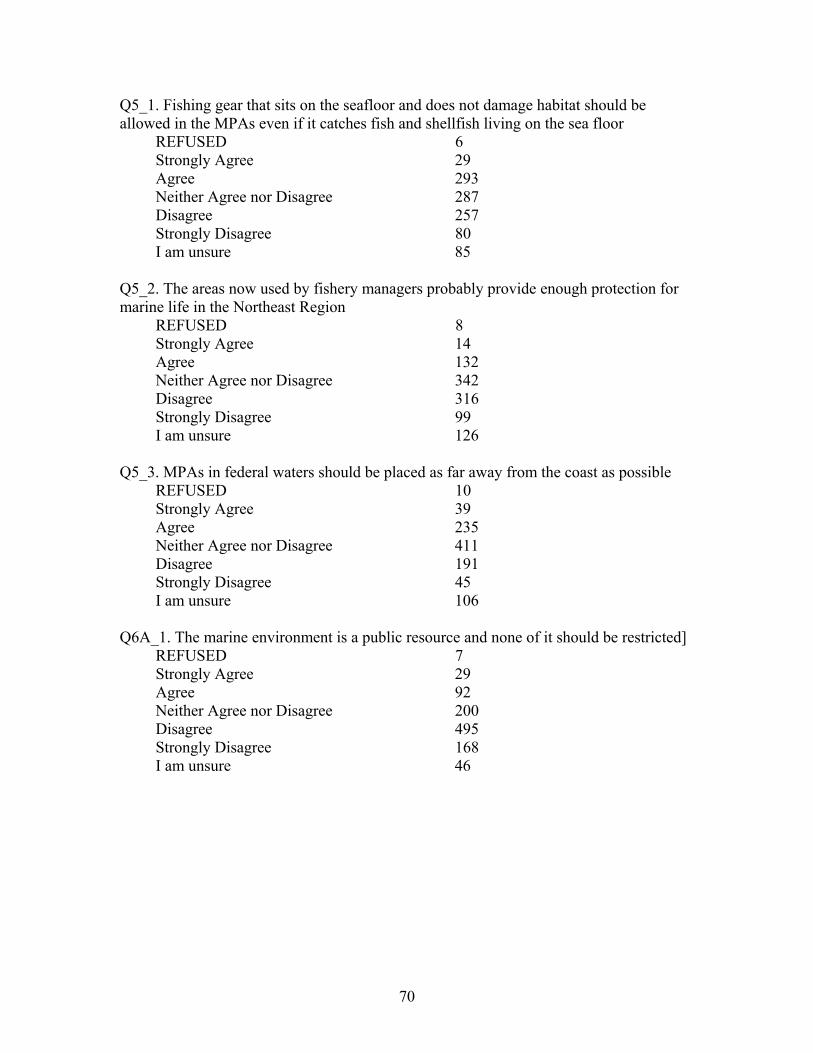
Q5_1. Fishing gear that sits on the seafloor and does not damage habitat should be allowed in the MPAs even if it catches fish and shellfish living on the sea floor REFUSED 6 Strongly Agree 29 Agree 293 Neither Agree nor Disagree 287 Disagree 257 Strongly Disagree 80 I am unsure 85 Q5_2. The areas now used by fishery managers probably provide enough protection for marine life in the Northeast Region REFUSED 8 Strongly Agree 14 Agree 132 Neither Agree nor Disagree 342 Disagree 316 Strongly Disagree 99 I am unsure 126 Q5_3. MPAs in federal waters should be placed as far away from the coast as possible REFUSED 10 Strongly Agree 39 Agree 235 Neither Agree nor Disagree 411 Disagree 191 Strongly Disagree 45 I am unsure 106 Q6A_1. The marine environment is a public resource and none of it should be restricted] REFUSED 7 Strongly Agree 29 Agree 92 Neither Agree nor Disagree 200 Disagree 495 Strongly Disagree 168 I am unsure 46

70

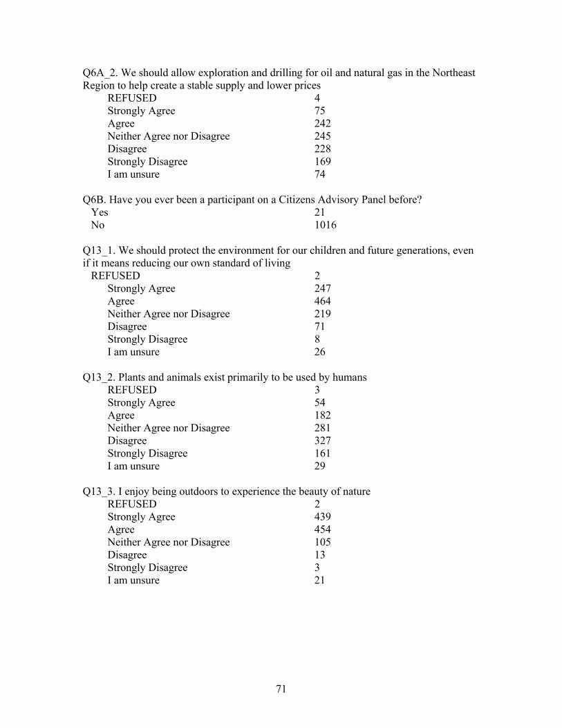
Q6A_2. We should allow exploration and drilling for oil and natural gas in the Northeast Region to help create a stable supply and lower prices REFUSED 4 Strongly Agree 75 Agree 242 Neither Agree nor Disagree 245 Disagree 228 Strongly Disagree 169 I am unsure 74 Q6B. Have you ever been a participant on a Citizens Advisory Panel before? Yes 21 No 1016 Q13_1. We should protect the environment for our children and future generations, even if it means reducing our own standard of living REFUSED 2 Strongly Agree 247 Agree 464 Neither Agree nor Disagree 219 Disagree 71 Strongly Disagree 8 I am unsure 26 Q13_2. Plants and animals exist primarily to be used by humans REFUSED 3 Strongly Agree 54 Agree 182 Neither Agree nor Disagree 281 Disagree 327 Strongly Disagree 161 I am unsure 29 Q13_3. I enjoy being outdoors to experience the beauty of nature REFUSED 2 Strongly Agree 439 Agree 454 Neither Agree nor Disagree 105 Disagree 13 Strongly Disagree 3 I am unsure 21

71

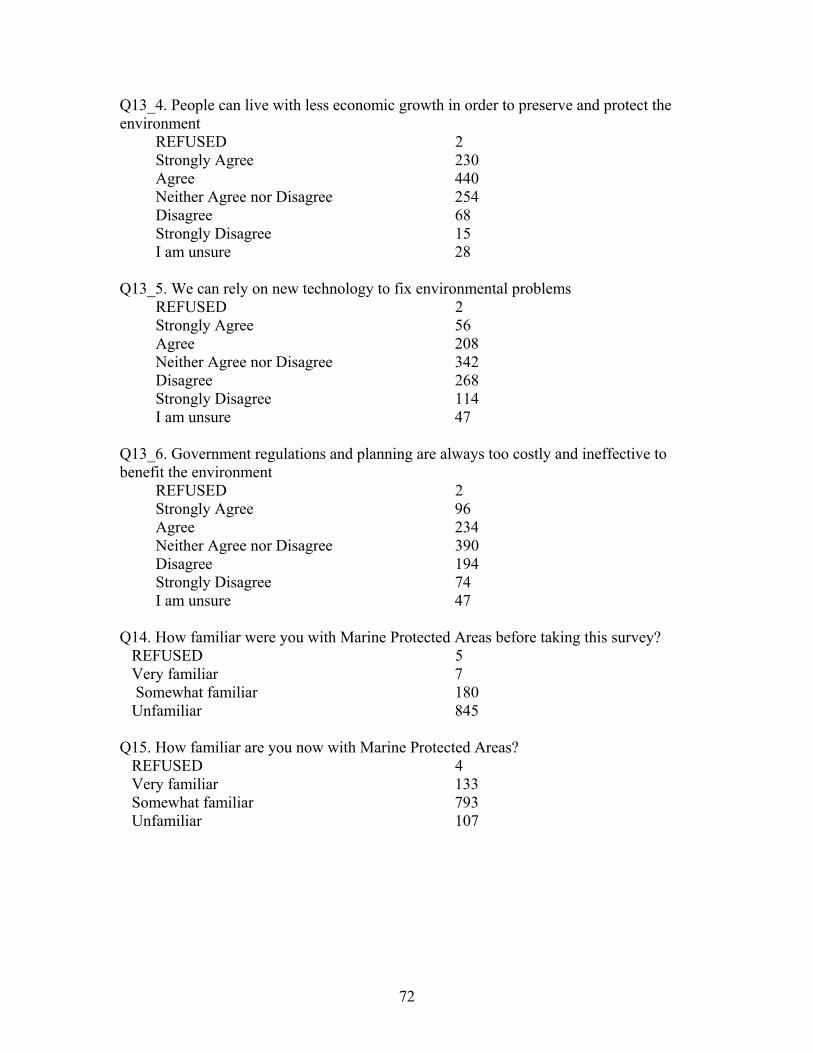
Q13_4. People can live with less economic growth in order to preserve and protect the environment REFUSED 2 Strongly Agree 230 Agree 440 Neither Agree nor Disagree 254 Disagree 68 Strongly Disagree 15 I am unsure 28 Q13_5. We can rely on new technology to fix environmental problems REFUSED 2 Strongly Agree 56 Agree 208 Neither Agree nor Disagree 342 Disagree 268 Strongly Disagree 114 I am unsure 47 Q13_6. Government regulations and planning are always too costly and ineffective to benefit the environment REFUSED 2 Strongly Agree 96 Agree 234 Neither Agree nor Disagree 390 Disagree 194 Strongly Disagree 74 I am unsure 47 Q14. How familiar were you with Marine Protected Areas before taking this survey? REFUSED 5 Very familiar 7 Somewhat familiar 180 Unfamiliar 845 Q15. How familiar are you now with Marine Protected Areas? REFUSED 4 Very familiar 133 Somewhat familiar 793 Unfamiliar 107

72