estimating climatological planetary boundary layer heights ... · estimating climatological...

Estimating climatological planetary boundary layer heightsfrom radiosonde observations: Comparison of methods anduncertainty analysis

Dian J. Seidel,1 Chi O. Ao,2 and Kun Li3

Received 8 December 2009; revised 14 April 2010; accepted 21 April 2010; published 25 August 2010.

[1] Planetary boundary layer (PBL) processes control energy, water, and pollutantexchanges between the surface and free atmosphere. However, there is no observation‐based global PBL climatology for evaluation of climate, weather, and air quality models orfor characterizing PBL variability on large space and time scales. As groundwork for sucha climatology, we compute PBL height by seven methods, using temperature, potentialtemperature, virtual potential temperature, relative humidity, specific humidity, andrefractivity profiles from a 10 year, 505‐station radiosonde data set. Six methods aredirectly compared; they generally yield PBL height estimates that differ by severalhundred meters. Relative humidity and potential temperature gradient methodsconsistently give higher PBL heights, whereas the parcel (or mixing height) method yieldssignificantly lower heights that show larger and more consistent diurnal and seasonalvariations (with lower nighttime and wintertime PBLs). Seasonal and diurnal patterns aresometimes associated with local climatological phenomena, such as nighttime radiationinversions, the trade inversion, and tropical convection and associated cloudiness.Surface‐based temperature inversions are a distinct type of PBL that is more common atnight and in the morning than during midday and afternoon, in polar regions than in thetropics, and in winter than other seasons. PBL height estimates are sensitive to thevertical resolution of radiosonde data; standard sounding data yield higher PBL heightsthan high‐resolution data. Several sources of both parametric and structural uncertainty inclimatological PBL height values are estimated statistically; each can introduceuncertainties of a few 100 m.

Citation: Seidel, D. J., C. O. Ao, and K. Li (2010), Estimating climatological planetary boundary layer heights from radiosondeobservations: Comparison of methods and uncertainty analysis, J. Geophys. Res., 115, D16113, doi:10.1029/2009JD013680.

1. Introduction

[2] The planetary boundary layer (PBL), the lowest por-tion of atmosphere, is of prime importance to climate,weather, and air quality. Processes within the PBL controlexchanges of momentum, water, and trace substancesbetween the Earth’s surface and the free troposphere, andthese processes are represented, often in parameterizedform, in atmospheric models. The structure of the PBL canbe complex and variable [Stull, 1988; Oke, 1988; Sorbjan,1989; Garratt, 1992], and the height (or depth) of thePBL is commonly used to characterize the vertical extent ofmixing within the boundary layer and the level at whichexchange with the free troposphere occurs [Bhumralkar,1976; Seibert et al., 2000; Medeiros et al., 2005].

[3] Traditionally, studies of the PBL have been highlylocalized and of relatively short duration. Although clima-tological analyses of PBL height have been undertaken forsome areas (e.g., for the United States by Holzworth [1964,1967]), a global climatology of PBL height has not beencompiled. In this study we explore some issues pertinent tothe development of such a climatology, which would haveapplications in (1) evaluation of the representation of thePBL in climate and air quality models; (2) interpreting PBLheights obtained in nontraditional ways, such as fromground‐based and space‐based lidar measurements ofaerosols, from boundary‐layer profiler observations, fromcloud base estimates from ceilometers, and from GlobalNavigational Satellite System (GNSS) radio occultationmeasurements; and (3) understanding the variability andlong‐term changes in PBL structure and related features,such as precipitable water, cloudiness, temperature andhumidity profiles, and atmospheric stability.[4] A global PBL height climatology will, perforce, be

based on automated algorithms applied to a very large dataset. Such an approach is distinctly different from the carefuland detailed examination of atmospheric profile data that

1NOAA Air Resources Laboratory (R/ARL), Silver Spring, Maryland,USA.

2Jet Propulsion Laboratory, California Institute of Technology,Pasadena, California, USA.

3University of Maryland, College Park, Maryland, USA.

Copyright 2010 by the American Geophysical Union.0148‐0227/10/2009JD013680

JOURNAL OF GEOPHYSICAL RESEARCH, VOL. 115, D16113, doi:10.1029/2009JD013680, 2010

D16113 1 of 15

http://dx.doi.org/10.1029/2009JD013680

can be made for local, micrometeorological PBL studies ofshort duration. The latter approach allows the investigatorto identify different types of boundary layers and complexfeatures, such as surface layers (also called inner layers orinertial sublayers), residual layers, and entrainment zones [e.g.,Stull, 1988; Garratt, 1992]. The main goals of this investiga-tion are to evaluate automated algorithms by applying severaldifferent PBL height definitions to a relatively large radiosondedata set, to compare the results, to quantify the uncertainty ofclimatological PBL height estimates, and to use these findingsto suggest optimal methods for developing useful global cli-matologies of PBL height. Section 2 describes the radiosondedata, the PBL height definitions, and the statistical tests used inthe comparison. Section 3 presents results in an objectivefashion and compares them with previous studies. Section 4discusses the results in the context of the overall goal ofdeveloping global climatologies, and section 5 presents thesummary.

2. Data and Methods

[5] This paper applies seven methods for estimating PBLheight to radiosonde data and compares the results usingstatistical tests, as described in this section.

2.1. Radiosonde Observations

[6] Daily observations from the global, land‐basedradiosonde station network for the 10 year period 1999–2008 were obtained from the Integrated Global RadiosondeArchive (IGRA) [Durre et al., 2006] (available at www.ncdc.noaa.gov). We used a special version of IGRA withenhanced information for studies of vertical structure [Durreand Yin, 2008] that includes the observed temperature,geopotential height, and humidity data at pressure levels, aswell as additional derived moisture variables and calculatedvertical gradients of several variables.

[7] Beginning with the full network of more than 1100stations, we restricted our analysis to 505 stations, shown inFigure 1, that met the following criteria:[8] 1. Soundings were accepted only if there were at least

10 upper air data levels at or below 500 hPa.[9] 2. At least 50% of the expected number of such

soundings were available for a given observation time andfor all four seasons (except in polar regions, where only oneseason was required).[10] On average, about 3030 soundings (83% of an ex-

pected 3653) were available for each station and time ofobservation selected for inclusion, and a total of more than2.2 million soundings were analyzed.[11] Most of the results presented here are based on

radiosonde data from the IGRA, which include data at thesurface, at standard (or mandatory) pressure levels (1000,925, 850, 700, 500 hPa, etc.), and at so‐called significantlevels at which the sounding deviates from linearity (inlogarithm of pressure) between two standard levels. Insection 3.4, we examine the effect of vertical resolution onPBL height estimates, using high‐resolution sounding datafor 1999–2007 (2008 was not available) from 44 U.S.‐operated stations (available from the Stratospheric Processesand their Role in Climate data center, www.sparc.sunysb.edu) [Wang and Geller, 2003].

2.2. Planetary Boundary Layer Height Estimates

[12] Seven different methods were used to estimate PBLheight in each sounding, as summarized in Table 1. Fourmethods are traditional approaches often encountered in thePBL literature. They include[13] 1. The “parcel method” [Holzworth, 1964; Seibert et

al., 2000], in which a mixing height is evaluated by com-paring the surface value of virtual potential temperature (Qv)to values aloft and identifying the height at which Qv is thesame as the surface value, and a hypothetical parcel of air,lifted from the surface, would be in equilibrium with its

Figure 1. Map of 505 radiosonde stations used in this study. The 44 U.S.‐operated stations shown in redhave high‐vertical‐resolution observations and were used to analyze the effect of vertical resolution onestimated PBL height.

SEIDEL ET AL.: CLIMATOLOGICAL BOUNDARY LAYER HEIGHTS D16113D16113

2 of 15

environment. The resulting PBL height is often called the“mixing height” and is commonly used in air pollution anddispersion studies to estimate the dilution of a pollutantreleased within the boundary layer. We evaluate the mixingheight at the time of the sounding and make no attempt toestimate the daily maximum value, which is sometimesdone using forecasts or observations of surface temperatureand humidity for application to air quality forecasts [e.g.,Holzworth, 1964], or the daily minimum value, whichprovides a worst‐case scenario for estimating surface con-centrations of pollutants released into the PBL.[14] 2. The level of the maximum vertical gradient of

potential temperature (Q) [Oke, 1988; Stull, 1988; Sorbjan,1989; Garratt, 1992], indicative of a transition from aconvectively less stable region below to a more stable regionabove.[15] 3. The base of an elevated temperature (T) inversion.

Not all soundings have elevated inversions, but whenpresent, the base serves as a cap to mixing below and so canbe considered the PBL height.[16] 4. The top of a surface‐based inversion (SBI)

[Bradley et al., 1993]. While the three methods above allowfor the possibility of an unstable or neutral PBL, a surface‐based T inversion is a clear indicator of a stable boundarylayer, whose top can define a PBL height. If an SBI is foundin a sounding, the other six methods are not evaluated, asthey assume a different PBL structure.[17] Three additional methods have recently been pro-

posed for identifying PBL height using GNSS radio occul-tation (RO) data, which can be used to derive verticalprofiles of atmospheric refractivity, temperature, and spe-cific humidity [Kursinski et al., 1997]. These methodsassume the PBL is a moister, denser, more refractive regionthan the overlying troposphere, and the PBL height is esti-mated as[18] 1. The level of the minimum vertical gradient of

specific humidity (q) [Ao et al., 2008].

[19] 2. The level of the minimum vertical gradient ofrelative humidity (RH).[20] 3. The level of the minimum vertical gradient of

refractivity (N) [Sokolovskiy et al., 2006; Basha andRatnam, 2009].[21] For the last of these, a refractivity profile is computed

from the temperature, pressure, and vapor pressure data[Smith and Weintraub, 1953]. Thus, we simulate GNSS ROprofiles with radiosonde data. (In a companion study, wewill directly compare PBL heights derived from GNSS ROdata and from radiosonde data, using identical algorithms.)[22] The reported surface level was not used in these

calculations; instead, we use the first reported upper air levelas a near‐surface observation. This was to avoid spuriousestimates of large vertical gradients resulting from hori-zontal (or vertical) separation of the surface instrumentshelter from the radiosonde launch site. In section 3.5 wequantify the effect of this decision by comparing climato-logical PBL height estimates obtained with and without thesurface level for a sample of stations.[23] For all methods, to avoid mistaking free tropospheric

features for the top of the PBL, if the PBL height was notfound in the lowest 4000 m, then it was considered missing.Thus, cases of deep convection, which may reach or evenpenetrate the tropopause, were not captured. To facilitatecomparison of climatological PBL heights from stations atdifferent elevations, all PBL heights are given in metersabove ground level (not above mean sea level).[24] We also attempted to evaluate PBL height using the

Richardson number (the dimensionless ratio of suppressionof turbulence by buoyancy to production of turbulence bywind shear). Although this method is frequently applied tomodel simulations, data limitations make it more difficult toapply to observations. The lack of wind data at the samelevels as the temperature and humidity data and the lack ofinformation with which to parameterize local surfaceroughness led to erratic and unreliable results, not included

Table 1. Methods for Estimating PBL Height and Percentage of Cases With Significant Seasonal Changes and Significant Diurnal Dif-ferences in Climatological Mean PBL Heighta

Abbreviation Method

SignificantSeasonal

Changes (%)Winter PBLLowest (%)

SignificantDiurnal

Differences (%)

NighttimePBL Lowest

(%)

Parcel Mixing height based on hypothetical verticaldisplacement of a parcel of air from thesurface and identification of the heightat which virtual potential temperature(Qv) is equal to the surface value.

83 50 87 76

Q Location of the maximum vertical gradient ofpotential temperature (Q)

92 51 72 42

q Location of the minimum vertical gradient ofspecific humidity (q)

87 49 67 23

RH Location of the minimum vertical gradient ofrelative humidity (RH)

88 60 62 28

N Location of the minimum vertical gradient ofrefractivity (N)

87 55 67 31

Elevated inversion Height of the base of an elevated temperatureinversion

94 50 72 43

Surface‐based inversionor SBI

Height of the top of a surface‐based temperatureinversion

n/a n/a n/a n/a

aOnly stations poleward of 30° latitude are included in the seasonal difference statistics, and only stations with nighttime data are included in the diurnaldifference statistics. Also shown are the percentages of those cases with significant seasonal and diurnal signals for which the lowest median PBL heights arefound in winter and at nighttime, respectively. Percentages are not shown for surface‐based inversions because the substantial seasonal and diurnal variationin their frequency of occurrence makes comparison of their mean heights problematic.


3 of 15

here. Other methods for estimating PBL height exist (seeSeibert et al. [2000] for a comprehensive review), but theyalso involve information not available from radiosondes,such as cloud base height, micrometeorological covariancestatistics, or turbulence flux profiles.

2.3. Statistical Tests and Uncertainty Estimates

[25] One important goal of this study is to quantify theparametric and structural uncertainty of climatological PBLheight estimates. Parametric, or value, uncertainty is asso-ciated with the necessity of using a finite sample of data toestimate population statistics. (See Thorne et al. [2005] for adiscussion of uncertainties in climate data sets.) We evaluatean aspect of parametric uncertainty in climatological medianPBL height values using interquartile ranges, as describedbelow. Structural uncertainty is associated with the meth-odology chosen in developing a data set from a set of ob-servations and is often ignored in climatological data setdevelopment. Here we evaluate the structural uncertainty inclimatological PBL height values associated with the choiceof PBL height estimation method and with radiosonde datachoices, using several statistical tests.[26] To evaluate the parametric uncertainty of climato-

logical values for a given method of estimating PBL height,computed PBL heights are binned according to station,3 month season (summer = December, January, and Februaryin the Southern Hemisphere; June, July, and August in theNorthern Hemisphere), and time of day. For each bin, wecalculate quartile values of PBL height as well as averagesand variances. Binning is a simple way to separate expectedatmospheric variability associated with the diurnal and sea-sonal cycles from sampling uncertainty (although weather‐related, within‐season variability will remain in the binneddata).[27] The diurnal variability of the PBL can be complex,

but discerning this variability with radiosonde data is achallenge, because soundings are generally made only onceor twice daily at fixed times (0000 and 1200 UTC). How-ever, they may be at any time of day or night depending onstation longitude and time of year. We binned the data intofour periods to capture the expected development of thePBL from stable nighttime conditions to convective condi-tions in afternoon, as follows: night (sunset to sunrise),morning (sunrise to solar noon), midday (noon to 3 h pastnoon), and afternoon (end of midday to sunset). Local timeof day relative to solar noon, sunrise, and sunset wascomputed for every sounding based on station latitude andlongitude. Thus, for the purposes of this paper, we defineclimatological PBL heights as the mean, or median, seasonal(or annual) value for a given station, portion of the day, andmethod, based on the 10 year period 1999–2008.[28] Structural uncertainty in climatological PBL heights

based on different methods is evaluated using five statisticaltests. We compare mean PBL heights with the Student’s ttest and PBL height variances with the F test. The Student’st test evaluates the null hypotheses that two samples (in thiscase, two sets of PBL height estimates based on two dif-ferent definitions) have consistent (not significantly differ-ent) means, based on the two sample means, variances, andsizes. Similarly, the F test uses these same parameters to testthe null hypothesis that the sample variances are consistent.In both cases, the P value (ranging from 0 to 1) indicates the

probability that differences as large as observed could occurby chance in samples with consistent means or variances, sothat a small P value can be interpreted as a statisticallysignificant difference in means (or variances): We take P ≤0.05 to indicate statistically significant differences.[29] Pearson’s linear correlation coefficient and the non-

parametric Spearman rank‐order correlation coefficient areused to measure the association of PBL heights based ondifferent methods and to test the null hypothesis that twosamples are uncorrelated. Both correlations can range from−1 to 1 (−100%–100%), and small P values indicate that thetwo samples are statistically significantly correlated. Wealso use the Komolgorov‐Smirnov test for differences incumulative distribution function, a nonparametric test basedon rank ordering of the data. The Kolmogorov‐Smirnov testevaluates the null hypothesis that two samples are drawnfrom the same distribution, using the test statistic D, theabsolute difference between two cumulative distributionfunctions. In this case small P values indicate statisticallysignificant differences between the samples.

3. Results

[30] Because surface‐based inversions (SBI) represent aseparate category of stable PBL for which the other sixmethods of estimating PBL height are not applicable, thissection first presents results related to the frequency andvariability of SBI. Next, we examine systematic differencesamong the remaining six methods and then discuss patternsof seasonal and diurnal variability of PBL height. We thenexamine the sensitivity of PBL height estimates to the ver-tical resolution of the soundings and to the choice regardinguse (or not) of the surface observations in radiosonde re-ports. Finally, we compare our findings with previousstudies.

3.1. Surface‐Based Inversions

[31] Figure 2 shows the frequency of occurrence of SBIsfor each station, as a function of station latitude. Nighttimeand morning (Figure 2, right) are clearly the times of day atwhich SBIs are likely to occur, and nighttime SBI frequencyranges from less than 50% at tropical stations up to about80% in polar regions. Typical frequencies during nighttimeand morning are about 40%. During midday and afternoon(i.e., from noontime until sunset, Figure 2, left), SBIs arerarer, with frequencies of less than 15% in the tropics andmidlatitudes, with higher values up to 50% in the polarzones.[32] The median height of the SBI is typically within 200–

500 m of the surface, with 25th and 75th percentile values ofabout 200 and 700 m, respectively (not shown). Thus, theSBI is a shallow layer, whose detection in radiosonde ob-servations often depends on the existence of “significant”level data and which may be difficult to observe using sat-ellite methods that do not penetrate the atmosphere to withina few hundred meters of the surface, such as GNSS RO.(See section 3.4 for more on the issue of vertical resolution.)The tops of SBIs are generally lower than the bases ofelevated inversions. The 25th and 75th percentile heights ofthe bases of elevated inversions are typically about 750 and2500 m, respectively.


4 of 15

[33] The SBI exhibits marked seasonal and diurnal vari-ability. For 53% of the 727 cases (505 stations, some withobservations at two different times of day), the highestfrequency of SBI occurrences is during winter, more thantwice the percentage expected by chance (25%, one seasonof four). Of the 505 stations in our analysis, 253 had SBI

observations available during both nighttime and one othertime of day, and 71% of that set exhibit a higher frequencyof SBI at night. These results are not surprising, as SBIstend to form in association with radiative cooling of thesurface, and it is encouraging to see this expected patternborne out in a 10 year radiosonde‐based climatology withlimited sampling of the diurnal cycle.

3.2. Systematic Differences Among Methods

[34] A fundamental purpose of this analysis is to deter-mine the robustness of estimates of climatological PBLheight and their sensitivity to the method chosen. Each of thesix remaining methods (excluding SBI) is based on verticalprofiles of different variables. Sometimes they yield identi-cal estimates of PBL height, as in the case of the 1100 UTC17 February 2007 sounding from Lerwick, UK (Figure 3,left). In this case four gradient‐based methods indicateidentical PBL heights of 2419 m, and an elevated inversionwas located just 31 m lower. The parcel method yields amixing height of 266 m, substantially lower than the otherestimates.[35] In contrast, we estimate five different values of PBL

height using the sounding of 2300 UTC 23 December 2006from the same station (Figure 3, right). They range from 219m for the parcel method to 2560 m for the specific humidityand relative humidity gradient methods. The high valuesobtained with the humidity methods in this case highlight adistinctive tendency of those methods in the presence ofclouds. Total cloud amount at the time of the sounding wasreported as 8 oktas with stratocumulus having base height of200 m (D. Hollis, UK Met Office, personal communication,2009). The mixing height of 219 m agrees well with the

Figure 3. Planetary boundary layer height estimates using six methods for Lerwick, United Kingdom,for (left) 1100 UTC 17 February 2007 and (right) 2300 UTC 23 December 2006. Profiles include tem-perature, potential temperature (Q), virtual potential temperature (Qv), relative humidity, specific humid-ity, and refractivity (N), some shifted for clarity. Estimated PBL heights are shown by dashed horizontallines. These soundings do not indicate the presence of surface‐based inversions.

Figure 2. Frequency of occurrence of surface‐based inver-sions (left) during midday and afternoon and (right) duringnighttime and morning as a function of station latitude.


5 of 15

depth of the layer below the cloud base, and the muchhigher PBL heights from the humidity methods might coin-cide with the top of the cloud deck. In contrast, the 1100 UTC17 February 2007 observation indicates cloud cover of3 oktas, which the sonde might well have missed during itsascent, so there is good agreement among the estimatesfrom different methods.[36] As an aside, we note that radiosonde humidity sensor

uncertainties may introduce systematic errors in PBL heightestimates in presence of cloud. If the humidity sensorproperly registers high humidity within the cloud and lowervalues above, both humidity methods will likely identify thecloud top as the PBL height. However, if there is a lag in thehumidity observations, a higher PBL height will be found.In either case, the resulting height is likely to be above theheights based on temperature or potential temperature,which may show sharper gradients at lower altitude, possi-bly at cloud base. Quantification of this source of uncer-tainty in PBL height estimates is beyond the scope of thisstudy.

[37] Figure 4 shows a gross comparison of PBL heightestimates from all seven methods. The data are separated bylocal time of day (as described in section 2.3), and each barrepresents the average over all stations of the annual cli-matological PBL height (the median over all observationsduring 1999–2008). Note that the SBI heights are based on adifferent set of soundings than all the other heights, andbecause some stations do not exhibit SBIs, data from fewerstations were used to compute SBI height average. Fur-thermore, elevated inversion base heights were not alwayspresent; on average, 13% of soundings had neither an ele-vated nor a surface‐based inversion. The parcel methodcould not be applied in about 0.1% of soundings in whichthe sounding had no value of Qv matching the near‐surfacevalue. Thus, the sample sizes for those two methods aresomewhat smaller than for the other four, which are basedon identical samples.[38] Typical average values of PBL height are between

200 and 2000 m, with SBI showing lowest values, as ex-pected. Among the other methods, PBL heights based on theRH gradient are consistently high, and those based on theparcel method are consistently low, differing by about afactor of 3 or 4, or more than 1 km. Disaggregated medianvalues reveal patterns consistent with the averages shown inFigure 4. Comparing climatological seasonal means forindividual stations and for specific parts of the day (2925cases in all), and not including the SBI heights, we findstatistically significant differences between methods yield-ing the lowest and highest values of PBL height in 99.8% ofthe cases. Heights based on the parcel method were over-whelmingly (96% of cases) the lowest, and heights based onRH and Q gradients were the highest (72% and 22% ofcases, respectively).[39] The possible effect of cloud cover, as illustrated in

the examples from Lerwick (Figure 3), may explain the highvalues obtained from RH profiles, which are sensitive tocloud top heights. The low values associated with the parcelmethod can be understood both in terms of the computa-tional algorithm and the underlying physical processes. Theparcel method algorithm seeks the first level at which Qv

matches the near‐surface value, whereas the other methodssearch the entire sounding for extrema in gradients, and theformer is more likely to be found at lower altitude thanthe latter [see, e.g., Stull, 1988, Figure 1.12]. Moreover, theeffective depth of atmospheric mixing within the boundarylayer, which depends on the buoyancy of parcels displacedfrom the surface, might well be below the level at which theprofile shows steepest gradients (for example, due to mid‐or high‐level clouds), irrespective of surface conditions.[40] The impact of the near‐surface Qv on PBL heights

from the parcel method is also a plausible explanation forthe stronger diurnal variation in those heights than fromother methods. (Note, however, that the four ensembles inFigure 4 are not based on the same stations, so they shouldnot be construed as a true representation of local diurnalvariation.) If PBL Qv profiles vary less than near‐surfacevalues and if near‐surface values diminish at night, themixing height estimate will perforce be lower at night, asseen in Figure 4, where average values increase fromnighttime to morning to midday to afternoon, when they arehighest. The average decrease in parcel method PBL heightfrom afternoon maximum to nighttime minimum is about

Figure 4. Average values (over all stations) of yearlymedian planetary boundary layer heights estimated usingseven different methods. (top to bottom) Results for morn-ing, midday, afternoon, and nighttime (see text for details).The number of stations used to compute each average (nstn)is shown; the first value applies to six methods and the sec-ond applies to surface‐based inversions.


6 of 15

170 m. The other methods do not show such pronounceddifferences.[41] Are these differences among methods statistically

significant? Table 2 shows results from each of the fivestatistical tests used to compare methods. For each part ofthe table, the percentage of cases for which the statistical testyielded a statistically significant result (P ≤ 0.05) is shownin the lower left corner, and the mean value of the teststatistic is shown in the upper right corner. The SBI resultsare not compared because of the different population ofsoundings used.[42] Overall, we find statistically significant correlations

among the methods in practically all comparisons (Table 2,c and d), with similar results for the Pearson and Spearmancorrelations. However, the correlation coefficients are low.Mean values (shown in the table) are ∼0.5 for comparisonsof the RH, Q, N, and q methods; ∼0.15 for comparisonsbetween those four methods and the parcel method; and ∼0for comparisons involving elevated T inversions. In thelatter case, mean correlation values close to zero, with anoverwhelming majority of statistically significant values, arethe consequence of averaging positive and negative signif-icant correlations.[43] The high percentages of statistically significant t, F,

and Kolmogorov‐Smirnov test results (Table 2, a, b, and e)reinforces the notion of significant differences amongmethods. The large t and F test values for comparisonsinvolving the parcel method are consistent with the muchlower PBL heights obtained with that method and the con-sequently lower means and variances. The high fraction ofstatistically significant test results is due to the large samplesizes used: The 10 year climatological values are based onaverage sample sizes of 3030 soundings (section 2.1).[44] The entries in Table 2 can be used to estimate the

structural uncertainty in climatological PBL heights asso-ciated with choice of method. The average differences inmean PBL height are several hundred meters for most of themethods compared and close to 1 km for comparisonsinvolving the parcel method. Thus, climatological averagescan have a structural uncertainty (Table 2) that is of order10%–100% of climatological mean values (e.g., Figure 4).

3.3. Seasonal and Diurnal Patterns

[45] Seasonal variations in PBL height should be easy todetect in radiosonde data because of excellent daily sam-pling throughout the year. Table 1 shows the percentage ofcases (a case being a station and a time of day) in whichthere are statistically significant differences in seasonalmean PBL heights (based on t tests), considering only sta-tions outside the tropical belt (i.e., poleward of 30° latitude).All of the methods are very sensitive to the seasonal cycle,with 83%–92% of cases showing a significant variation.However, the nature of the seasonal variation is not con-sistent, either from station to station or from method tomethod. The fraction of cases with significant seasonalchanges that also have lowest seasonal median PBL heightsin winter is about 50%. (We have already seen, in section3.1, that SBI frequencies are also greatest in winter.)[46] While spatial differences in seasonal PBL height

changes can be explained (and will be illustrated below),that different methods sometimes show different seasonalvariations for a given station and time of day suggests again

Table 2. Results of Five Statistical Tests Comparing Six Methodsfor Estimating PBL Heighta

(a) Difference in means (m)

Parcel Q q RH N Elevated Inversion

Parcel ‐ 1197 1104 1354 952 751Q 100 ‐ −92 156 −244 −440q 100 76 ‐ 249 −152 −343RH 100 80 96 ‐ −401 −594N 100 87 88 99 ‐ −191Elevated inversion 100 99 93 98 88 ‐

(b) Ratio of variances


Parcel ‐ 10.9 11.0 11.5 10.3 8.8Q 100 ‐ 1.1 1.1 1.1 1.3q 100 49 ‐ 1.1 1.1 1.4RH 100 40 43 ‐ 1.2 1.4N 100 45 32 66 ‐ 1.3Elevated inversion 100 76 78 81 71 ‐

(c) Pearson linear correlation coefficient (%)


Parcel ‐ 18 10 12 14 1Q 100 ‐ 37 49 41 4q 99 100 ‐ 67 60 0RH 100 100 100 ‐ 52 0N 100 100 100 100 ‐ 0Elevated inversion 96 97 96 96 96 ‐

(d) Spearman correlation coefficient (%)


Parcel ‐ 19 12 12 17 2Q 99 ‐ 37 50 42 1q 99 100 ‐ 66 60 0RH 100 100 100 ‐ 51 1N 99 100 100 100 ‐ 1Elevated inversion 97 96 97 96 96 ‐

(e) Kolmogorov‐Smirnov D statistic


Parcel ‐ 0.64 0.61 0.63 0.56 0.48Q 100 ‐ 0.11 0.9 0.12 0.21q 100 88 ‐ 0.10 0.80 0.21RH 100 84 83 ‐ 0.17 0.27N 100 92 87 99 ‐ 0.16Elevated inversion 100 100 98 100 96 ‐

aEach section of the table shows average values of the relevant teststatistic in the upper right corner, and the percentages of cases for whichthe test yielded statistically significant results (P = 0.05) in the lower leftcorner. Each table entry represents 740 comparison cases, with one casebeing all the PBL height values for 1999–2008 from a single station andpart of the day. The statistics are the (a) difference in mean PBL heightevaluated with Student’s t test, (b) ratio of PBL height variancesevaluated with the F test, (c) Pearson linear correlation coefficient,(d) Spearman rank‐order correlation coefficient, and (e) D statistic fromthe Kolmogorov‐Smirnov test of differences in distribution functions ofPBL heights (representing the maximum value of the absolute differencebetween two cumulative probability distribution functions). Note thathigh percentages of statistically significant results (values near 100% inthe lower left corners) indicate statistically significant differences in mostof the test cases for the Student’s t test, the F test, and the Kolmogorov‐Smirnov test, whereas they indicate significant correlations in most casesfor the two correlation tests.


7 of 15

that they cannot be viewed as surrogates for one another.Seasonal variations, when significant, tend to be severalhundred meters, with a median value of 440 m and inter-quartile range of 210–750 m. This is comparable to themagnitude of the structural uncertainty in mean PBL heightestimates discussed above, which complicates efforts todistinguish true seasonal variations from effects associatedwith choice of PBL height method.[47] Radiosonde data are not well suited to analysis of

diurnal variations because observations are made only 1 or 2(or at a few stations four) times daily. However, we haveattempted an analysis of day/night differences for those 275of the 505 stations at which the comparison is possible.Table 1 indicates the percentage of cases with significantdifferences in PBL height between nighttime and one of thethree other parts of the diurnal cycle (see section 2.3 on

partitioning of the day), with most cases showing a signif-icant difference. The parcel method shows a significantdifference for 87% of the stations, and the overwhelmingtendency (76% of the significant cases) is for lower PBLheights at nighttime. The other six methods show somewhatsmaller percentages of stations (62%–72% of cases) withsignificant differences and a much weaker tendency forlower nighttime PBL heights. Considering all methods,median day/night differences are about 210 m, with an in-terquartile range of 100–420 m. Although slightly smallerthan typical seasonal variations, these diurnal changes arealso comparable in magnitude to the structural uncertaintyof PBL height estimates. Recall that SBI frequency ofoccurrence is much greater at night (Figure 2).[48] Examples of the seasonal and diurnal variations in

PBL height at four sample stations are shown in Figures 5,6, 7, and 8, which also illustrate differences among theseven methods. The observations at Prague, Czech Republic(Figure 5), show the presence of SBIs in 24% of soundingsat night (Figure 5, bottom) but only in 12% of middaysoundings (Figure 5, top). The top of the SBI is low (medianheight 539 m in the afternoon and 413 m at night) and variesrelatively little (interquartile ranges are 292 and 308 m,respectively). When SBIs are not found, the PBL height

Figure 5. Seasonal and annual quartile values of planetaryboundary layer height (m above ground level) at Prague,Czech Republic (50°N, 14°E), based on data for 1999–2008. For each method, the 25th, 50th, and 75th percentilevalues are shown (in colored, white, and gray bars, respec-tively), for (top) midday and (bottom) nighttime. Heightsbased on surface‐based inversions are from a different setof soundings than heights based on the other methods. Theyare not shown for daytime for some seasons at Praguebecause they occur rarely (1% of soundings).

Figure 6. Same as Figure 5 but for Oakland, California(38°N, 122°W), for afternoon and nighttime.


8 of 15

estimates are generally much higher, with median heightsfor all but the parcel method of about 1500–2200 m, andmuch more variable. They show seasonal variation, withstatistically significantly higher values in summer and lowervalues in winter for all methods except the parcel and SBI.The most salient diurnal patterns are the much lower mixingheights (from the parcel method) at night than at midday(with median heights of 597 and 851 m, respectively). Othermethods show the opposite diurnal pattern (higher PBL atnight) but not consistently for all methods or seasons. Thisdifferent behavior of day/night patterns is a clear indicationthat the gradient methods are not sensitive to the samediurnal variations as the parcel method and therefore areindicators of different PBL processes.[49] Much lower PBL heights and a much different sea-

sonal cycle are seen at Oakland, California (Figure 6), wheremedian PBL heights are over 1000 m in winter and about500 m in summer, when subsidence inversions associatedwith the Pacific high‐pressure system dominate the region.All six non‐SBI methods show lowest heights in summer,highest in winter, and statistically significant differencesbetween them. As at Prague, SBIs are rarer in the daytime(afternoon in this case) than at night (13% versus 30%frequency of occurrence).[50] Morning PBL heights at Antofagasta, Chile (where

nighttime data are not available), are about 900 m, aregenerally higher in summer than winter, and show littlevariability within a given season (Figure 7). The area isinfluenced by the trade inversion [Hastenrath, 1991], whichappears to cause a well‐defined PBL. About 21% ofsoundings show SBIs. The q, RH, and N methods give PBLheight distribution and mean values that are in betteragreement than at other stations, probably because of thedominating effect of the trade inversion on the verticalprofile of these moisture/density parameters. The parcelmethod gives lower values and a distribution that is signif-icantly different from these others.[51] As a final example, Majuro Atoll in the Marshall

Islands (Figure 8) shows the high (typically above 2000 m)PBL heights and flat seasonal structure expected in the deeptropics. Both midday and at night, SBIs were found in only

1% of cases. Parcel method mixing heights are much lowerthan the PBL heights estimated using the other methods(about 800 versus 2000 m, respectively), both midday andnighttime. While parcel method heights are significantlylower at night than midday for all seasons, the oppositepattern prevails for the q, RH, and N methods, although lessconsistently from season to season.[52] As these examples demonstrate, there is considerable

diversity among stations in seasonal and diurnal patterns ofPBL height variations. These can sometimes be explained interms of prevailing climatic conditions associated with theglobal general circulation of the atmosphere. Nevertheless,the main systematic features discussed in the precedingsection are fairly robust.

3.4. Sensitivity to Vertical Resolution of Sounding Data

[53] The analysis presented above is based on standard‐resolution radiosonde data, as transmitted from stations foruse in numerical weather prediction, which may include asfew as three or four mandatory data points within the PBL(surface and 1000, 925, 850, 700, 500 hPa). Additionalsignificant level reports should be included if the structureof the atmosphere is such that interpolation between the

Figure 8. Same as Figure 5 but for Majuro Atoll, MarshallIslands (7°N, 171°E), at midday and nighttime.

Figure 7. Same as Figure 5 but for Antofagasta, Chile(22°S, 137°W), for morning only.


9 of 15

mandatory levels would not reproduce the sounding. Asmentioned in section 2.1, we required at least 10 data levelsat or below 500 hPa for the IGRA data used in this study;the average number (over all soundings during 1999–2008)ranged (over all stations) from 11 to 34 levels, with a net-work average of 16 levels. In contrast, high‐resolution dataare reported at regular time intervals during the sounding,and their vertical resolution is about an order of magnitudegreater than in the standard‐resolution IGRA.[54] Figure 9 compares the high‐resolution and standard‐

resolution sounding reports for 1200 UTC on 21 February2007 from Koror, Republic of Palau, to illustrate thepotential impact of vertical resolution on estimated PBLheight. Between the surface and 4 km, the standard reportincludes 19 levels, whereas the high‐resolution report has127, with the latter showing more fine structure in the rel-ative humidity profile (Figure 9, right) than the former. Theq, N, and Q gradient methods yield identical PBL heights(1114 m) from both reports. However, the minimum RHgradient occurs at 3715 m in the standard‐resolution IGRAsounding and at 1114 m in the high‐resolution sounding.The parcel and elevated inversion methods also give dif-ferent results: 1098 and 116 m, respectively, in the high‐resolution data versus 1057 and 767 m, respectively, in thestandard‐resolution data.[55] To test the overall sensitivity of climatological PBL

height results to the vertical resolution of the sounding, weapplied the same methods for estimating PBL height and forcomputing climatological statistics to paired sounding re-ports from 44 stations (in the United States and a smallnumber of Caribbean and Pacific islands) for which both

standard and high‐resolution data were available (Figure 1)for 1999–2007. Figures 10 and 11 illustrate the level ofagreement between the standard and high‐resolution resultsfor each of the PBL height estimation methods.[56] Although it may not be visually apparent in the fig-

ures, there are statistically significant differences betweenstandard and high‐resolution results for most cases. The bestagreement is for the RH and Q methods, for which soundingresolution has no statistically significant effect on mean PBLheight at about half the stations tested. For all of the othermethods, and at almost all the stations, the choice ofsounding resolution results in statistically significant dif-ferences in mean values, with differences up to several 100m. In general, we obtain lower PBL heights from the high‐resolution data. This result is expected for the parcel andtemperature inversion (both elevated T inversion and SBI)methods, which involve a search for the first instance(working upward from the surface) of Qv matching the nearsurface value, or of a change in the sign of the temperaturelapse rate, respectively. These conditions are more likely tobe found lower in the atmosphere when more data levelsare available, as in the Koror example discussed above(Figure 9). The frequency of finding SBIs is not very sen-sitive to sounding resolution (Figure 11, middle and bottom).The frequency estimates from both sets of soundings aretypically within 5%.[57] Thus, it appears that, although standard‐resolution

sounding data contain sufficient information to allow iden-tification of PBL height, the estimated height is sensitiveto the number of data levels available. Use of standard‐resolution sounding data yields higher PBL heights than

Figure 9. Effect of sounding vertical resolution on estimated PBL heights (m) at Koror Island, Republicof Palau (7°N, 134°E), for the 1200 UTC sounding of 21 February 2007. Standard‐resolution and high‐resolution (black and red curves, respectively) (left) temperature (K) and (right) relative humidity (%)soundings are shown, along with the PBL heights identified by six methods. For the parcel, elevatedinversion, and RH gradient methods, estimated heights differ for the high‐resolution and standard‐resolution cases. For the q, N, and Q gradient methods, estimated PBL heights are the same.


10 of 15

high‐resolution data and can introduce structural uncertaintiesof a few 100 m in climatological means.

3.5. Sensitivity to Surface‐Level Observations

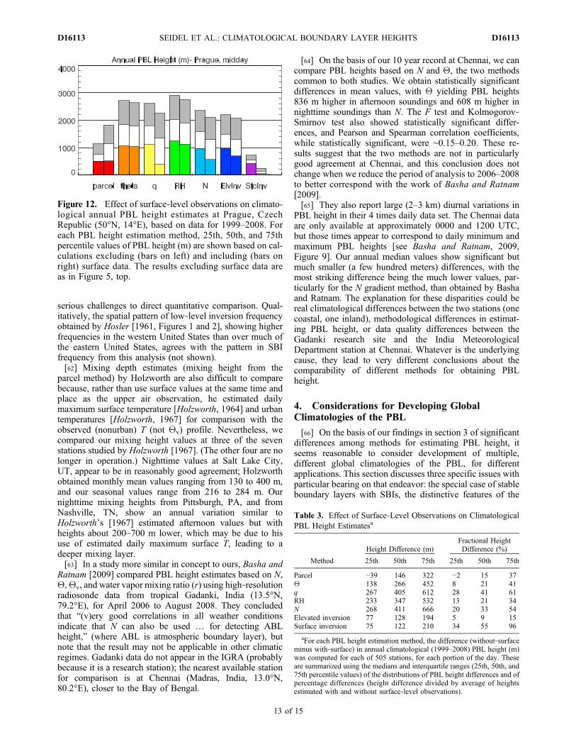
[58] A related source of structural uncertainty is ourdecision to ignore the surface‐level data in estimating PBLheight, as discussed in section 2.2. Figure 12 comparesestimated annual climatological PBL heights from Prague,Czech Republic, both including and excluding the surfaceobservations. (The results excluding the surface are the sameas those shown in Figure 5, top, for the year.) While allseven methods are sensitive to the inclusion of surface data(and the t test confirms statistically significant differences in

10 year mean values), the most striking differences are forthe parcel and surface‐based inversion methods, as would beexpected, since both of these methods are strongly depen-dent on the surface (or assumed‐surface) data.[59] Table 3 shows a summary of the results of this

comparison applied to the 505‐station network. For eachmethod, the median and interquartile range of the differencein climatological PBL height estimated with and withoutsurface‐level data measure this source of structural uncer-tainty. The most striking feature of the results is that thedifferences are generally positive, i.e., PBL heights obtainedwithout including the surface observation are higher. This isexpected for the parcel and SBI methods because they

Figure 10. Comparison of 25th, 50th and 75th percentile values of PBL heights (m) from 44 stationsbased on standard (blue) and high (red) vertical resolution sounding data, as a function of station latitude.Each frame shows results for a different method of estimating PBL height using observations for 1999–2007. Note the different vertical axis scale for the parcel method (lower left frame).


11 of 15

depend directly on the lowest data level. That the gradientmethods also yield this result suggests that the strongestgradients are frequently found between the surface and thefirst level above the surface. This finding could be inter-preted as a confirmation of the potential for unrepresentativegradients because of noncollocation of the surface and upperair observations, which was our reason for omitting thesurface observations in most of our analyses.[60] The magnitude of the differences in climatological

means is several hundred meters (Table 3), with thehumidity and refractivity methods showing the most sensi-tivity, due to strong near‐surface humidity gradients. Ex-pressed as a fraction of climatological mean PBL height, thissource of structural uncertainty is typically about 10%–30%for the six non‐SBI methods (Table 3). Thus, the effect of

surface observations introduces uncertainty that is compa-rable in magnitude to the effect of vertical resolution ofsounding data (section 3.4).

3.6. Comparison With Prior Studies

[61] To our knowledge, there are few prior studies ofclimatological PBL heights on global or even regionalscales. We have attempted to compare our SBI and mixingheight (parcel method) results for U.S. stations with those ofHosler [1961] and of Holzworth [1964, 1967], respectively,who analyzed radiosonde data from continental U.S. sta-tions. However, differences in the location of stations in theradiosonde network, standard observing times, analysismethod, period of record, and assumptions, as well as thelack of digital data records from these early studies, posed

Figure 11. (top) Same as Figure 10, but showing results for the height of the top of surface‐basedinversions (SBI). (middle) Frequency (%) of SBI occurrence based on standard (blue) and high verticalresolution (red) data. (bottom) Difference (standard minus high resolution) in SBI frequency.


12 of 15

serious challenges to direct quantitative comparison. Qual-itatively, the spatial pattern of low‐level inversion frequencyobtained by Hosler [1961, Figures 1 and 2], showing higherfrequencies in the western United States than over much ofthe eastern United States, agrees with the pattern in SBIfrequency from this analysis (not shown).[62] Mixing depth estimates (mixing height from the

parcel method) by Holzworth are also difficult to comparebecause, rather than use surface values at the same time andplace as the upper air observation, he estimated dailymaximum surface temperature [Holzworth, 1964] and urbantemperatures [Holzworth, 1967] for comparison with theobserved (nonurban) T (not Qv) profile. Nevertheless, wecompared our mixing height values at three of the sevenstations studied by Holzworth [1967]. (The other four are nolonger in operation.) Nighttime values at Salt Lake City,UT, appear to be in reasonably good agreement; Holzworthobtained monthly mean values ranging from 130 to 400 m,and our seasonal values range from 216 to 284 m. Ournighttime mixing heights from Pittsburgh, PA, and fromNashville, TN, show an annual variation similar toHolzworth’s [1967] estimated afternoon values but withheights about 200–700 m lower, which may be due to hisuse of estimated daily maximum surface T, leading to adeeper mixing layer.[63] In a study more similar in concept to ours, Basha and

Ratnam [2009] compared PBL height estimates based on N,Q,Qv, and water vapor mixing ratio (r) using high‐resolutionradiosonde data from tropical Gadanki, India (13.5°N,79.2°E), for April 2006 to August 2008. They concludedthat “(v)ery good correlations in all weather conditionsindicate that N can also be used … for detecting ABLheight,” (where ABL is atmospheric boundary layer), butnote that the result may not be applicable in other climaticregimes. Gadanki data do not appear in the IGRA (probablybecause it is a research station); the nearest available stationfor comparison is at Chennai (Madras, India, 13.0°N,80.2°E), closer to the Bay of Bengal.

[64] On the basis of our 10 year record at Chennai, we cancompare PBL heights based on N and Q, the two methodscommon to both studies. We obtain statistically significantdifferences in mean values, with Q yielding PBL heights836 m higher in afternoon soundings and 608 m higher innighttime soundings than N. The F test and Kolmogorov‐Smirnov test also showed statistically significant differ-ences, and Pearson and Spearman correlation coefficients,while statistically significant, were ∼0.15–0.20. These re-sults suggest that the two methods are not in particularlygood agreement at Chennai, and this conclusion does notchange when we reduce the period of analysis to 2006–2008to better correspond with the work of Basha and Ratnam[2009].[65] They also report large (2–3 km) diurnal variations in

PBL height in their 4 times daily data set. The Chennai dataare only available at approximately 0000 and 1200 UTC,but those times appear to correspond to daily minimum andmaximum PBL heights [see Basha and Ratnam, 2009,Figure 9]. Our annual median values show significant butmuch smaller (a few hundred meters) differences, with themost striking difference being the much lower values, par-ticularly for the N gradient method, than obtained by Bashaand Ratnam. The explanation for these disparities could bereal climatological differences between the two stations (onecoastal, one inland), methodological differences in estimat-ing PBL height, or data quality differences between theGadanki research site and the India MeteorologicalDepartment station at Chennai. Whatever is the underlyingcause, they lead to very different conclusions about thecomparability of different methods for obtaining PBLheight.

4. Considerations for Developing GlobalClimatologies of the PBL

[66] On the basis of our findings in section 3 of significantdifferences among methods for estimating PBL height, itseems reasonable to consider development of multiple,different global climatologies of the PBL, for differentapplications. This section discusses three specific issues withparticular bearing on that endeavor: the special case of stableboundary layers with SBIs, the distinctive features of the

Table 3. Effect of Surface‐Level Observations on ClimatologicalPBL Height Estimatesa

Method

Height Difference (m)Fractional HeightDifference (%)

25th 50th 75th 25th 50th 75th

Parcel −39 146 322 −2 15 37Q 138 266 452 8 21 41q 267 405 612 28 41 61RH 233 347 532 13 21 34N 268 411 666 20 33 54Elevated inversion 77 128 194 5 9 15Surface inversion 75 122 210 34 55 96

aFor each PBL height estimation method, the difference (without‐surfaceminus with‐surface) in annual climatological (1999–2008) PBL height (m)was computed for each of 505 stations, for each portion of the day. Theseare summarized using the medians and interquartile ranges (25th, 50th, and75th percentile values) of the distributions of PBL height differences and ofpercentage differences (height difference divided by average of heightsestimated with and without surface‐level observations).

Figure 12. Effect of surface‐level observations on climato-logical annual PBL height estimates at Prague, CzechRepublic (50°N, 14°E), based on data for 1999–2008. Foreach PBL height estimation method, 25th, 50th, and 75thpercentile values of PBL height (m) are shown based on cal-culations excluding (bars on left) and including (bars onright) surface data. The results excluding surface data areas in Figure 5, top.


13 of 15

mixing height, and issues relevant to combining radiosondedata with Global Navigation Satellite System RadioOccultation observations.

4.1. Special Case of Surface‐Based Inversions

[67] Although the analysis presented above does notspecifically address measures of PBL stability (such as lapserates), surface‐based temperature inversions are a clearindication of a stable layer. The prevalence of SBIs, par-ticularly at night and in the polar regions, and the incom-patibility of SBI with the other six methods of determiningPBL height explored here, suggest that separate consider-ation of the climatology of SBIs may be warranted. Bradleyet al. [1993], focusing on Arctic SBIs, and Bourne et al.[2010], focusing on Alaska, outline compelling reasons forin‐depth analysis of this type of especially stable PBL inwhich mixing is confined to a shallow layer and the PBL iseffectively decoupled from the free troposphere. The largediurnal signal in SBI occurrence frequency provides a strongrationale for directly addressing diurnal variations in anyPBL climatology. One potential area of concern is thedependence of SBI frequency and height both on the sur-face‐level data (section 3.5) and on the vertical resolution ofthe archived sounding data (section 3.4), which suggeststhat high‐resolution data may be more suitable than standardresolution for SBI analysis.

4.2. Distinctive Features of the Mixing Height

[68] If detailed PBL turbulence and surface roughnessinformation is not available (as is likely the case for anyglobal data set from which PBL climatologies might bedeveloped), air quality studies might tend to favor themixing height, based on the parcel method, as an indicationof the potential atmospheric ventilation and dilution ofpollutants emitted from the surface. As we have seen,mixing height statistics have unique features in comparisonwith the other methods we have examined. Mixing heightsare lower than, and poorly correlated with, the other PBLheight estimates, exhibit greater diurnal changes with moreconsistent low values at night, and can show different sea-sonal changes. For these reasons, climatologies of parcelmethod mixing heights appear warranted, specifically for airquality applications. Given the spatial sampling of theradiosonde network (Figure 1), mixing height climatologiesfor Europe, Australia, and the United States might beattempted. As with SBIs, the dependence of mixing heighton sounding vertical resolution (and the tendency to obtainlower heights from higher resolution data) will complicatethe analysis.

4.3. Issues Relevant to Global Navigation SatelliteSystem Radio Occultation Observations

[69] To evaluate newly proposed methods of evaluatingPBL height from GNSS RO observations, we included thosebased on vertical gradients of specific humidity, relativehumidity, and refractivity in our study. Using radiosondedata to obtain refractivity profiles, we find that these threemethods tend to yield more similar results than the otherfour, more traditional, methods we examined. Nevertheless,the agreement among them remains poor. They yield higherPBL heights than the others; are only moderately well cor-

related (r ∼ 0.5); and more often than not show statisticallysignificantly different means, variances, and distributionfunctions.[70] Nevertheless, because GNSS RO data are (and will

be) available in regions and for times of day that radiosondeobservations are lacking, it seems worthwhile to furtherevaluate their potential, either independently or in combi-nation with other data sources, to provide a global PBLclimatology. Therefore, we intend to make direct compar-isons of PBL heights based on actual GNSS RO data withthose derived from radiosonde profiles. However, it isimportant to recognize that some features of the PBL will bevery difficult, if not impossible, to delineate with GNSS ROobservations. These include surface‐based inversions andshallow boundary layers because of the degradation ofGNSS RO profiles at low altitudes above the surface.

5. Summary

[71] This paper lays the groundwork for development of aglobal climatology of the planetary boundary, which, to ourknowledge, has not previously been attempted with radio-sonde or other observations. Using a 10 year, 505‐stationglobal radiosonde data set, we have compared seven meth-ods of computing PBL height and have attempted to quan-tify aspects of the structural and parametric uncertainty inclimatological values. The main findings are[72] a. Surface‐based inversions are a distinct type of

PBL; when they are present, the other six methods were notapplied. They are more common at night and in the morning(i.e., sunset to noon) than during midday and afternoon,more common in polar regions than in the tropics, and morecommon in winter than other seasons. The top of the SBI istypically between 200 and 700 m (typical 25th and 75thpercentile values).[73] b. The other six methods (based on vertical gradients

of T, RH, q, N, and Q, and based on the parcel methodinvolving Qv) generally yield different estimates of clima-tological PBL height.[74] (i) The parcel (or mixing height) method consistently

yields significantly lower heights than the other methodsand exhibits larger and more consistent diurnal and seasonalvariations, with lower values at night and in winter.[75] (ii) The RH and Q gradient methods consistently

yield higher PBL height estimates than the others.[76] (iii) Methods based on finding maximum or mini-

mum vertical gradients (of RH, q, N, or Q) are in betteragreement than those based on locating elevated T inver-sions or on the mixing height. However, in the majority ofcases, there are statistically significant differences (in cli-matological mean values, variances, and cumulative dis-tribution functions) among all the methods. Correlationsamong methods are statistically significant but small(generally less than 0.5, with some significant negativecorrelations).[77] (iv) Specifically, PBL height based on refractivity (N)

gradients, such as those that may be obtained from GNSSradio occultation observations, are not equivalent to thosebased on gradients in other meteorological parameters.[78] c. Seasonal and diurnal patterns of PBL height vari-

ability differ from station to station and can sometimes be


14 of 15

interpreted in terms of climatological phenomena, such asnighttime radiation inversions, the trade inversion, andtropical convection and associated cloudiness.[79] d. Climatological PBL heights are subject to both

parametric, or sampling, uncertainty and structural uncer-tainty associated with methodological choices. Typicalmagnitudes of these uncertainties are several hundred meters.[80] (i) The parametric uncertainty of 10 year climatolog-

ical PBL heights for a given station, season, time of day, andmethod can be characterized by the interquartile range aboutthe median, which range from a few hundred meters to morethan 1 km. This sampling uncertainty encompasses PBLchanges associated with day‐to‐day weather variability.[81] (ii) Three sources of structural uncertainty are choice

of PBL height estimation method, vertical resolution ofsounding data, and inclusion or exclusion of surface‐levelobservations in estimating climatological PBL heights. Eachof these introduce uncertainties of order several hundredmeters. The effects of these choices tend to be systematicrather than random. Lower PBL heights are associated withthe parcel method than the gradient methods, with high‐resolution rather than standard‐resolution sounding data,and with including rather than excluding the surfaceobservation.[82] (iii) These uncertainties are important to consider in

comparing radiosonde‐based climatological estimates withthose from models and from other observing systems.[83] e. Because of the substantial sensitivity of PBL

heights to estimation method, there is merit in separate cli-matological analyses for specific purposes. Because of itsimportance in air quality modeling, mixing height based onthe parcel method is an obvious choice for PBL climatolo-gies, particularly over the relatively well‐sampled anddensely populated continents. In the polar regions, cli-matologies of surface‐based inversion characteristics andfrequencies of occurrence would aid in evaluating the role ofthis common PBL type in high‐latitude climate processes.Other methods may be better suited to climatologies de-signed for comparisons with climate models or with otherobserving systems.

[84] Acknowledgments. We thank Angela Betancourt‐Negron(University of Puerto Rico) for assistance with data processing and DanHollis (UK Met Office) for providing cloud observations for Lerwick.Yehui Zhang (NOAA Air Resources Laboratory) performed calculationsto test the effects of including surface‐level observations. Julian Wangand Donald Ballard (NOAA Air Resources Laboratory), Imke Durre(NOAA National Climatic Data Center), Venkat Ratnam, (National Atmo-spheric Research Laboratory, Gadanki), and four anonymous reviewerseach provided helpful suggestions on the manuscript. Research performedby C. Ao was carried out at the Jet Propulsion Laboratory, CaliforniaInstitute of Technology, under a contract with the National Aeronauticsand Space Administration.

ReferencesAo, C. O., T. K. Chan, B. A. Iijima, J.‐L. Li, A. J. Mannucci, J. Teixeira,B. Tian, and D. E. Waliser (2008), Planetary boundary layer informa-tion from GPS radio occultation measurements. GRAS SAF Workshop

on Applications of GPSRO Measurements, 16–18 June 2008, 123–131.(Available at http://www.grassaf.org/Workshops/agrom_prog/Ao.pdf).

Basha, G., and M. V. Ratnam (2009), Identification of atmospheric bound-ary layer height over a tropical station using high resolution radiosonderefractivity profiles: Comparison with GPS radio occultation measure-ments, J. Geophys. Res., 114, D16101, doi:10.1029/2008JD011692.

Bhumralkar, C. M. (1976), Parameterization of the planetary boundarylayer in atmospheric general circulation models, Rev. Geophys., 14,215–226.

Bourne, S. M., U. S. Bhatt, J. Zhang, and R. Thoman (2010), Surface‐basedtemperature inversions in Alaska from a climate perspective, Atmos. Res.,95, 353–366, doi:101016/j.atmosres.2009.09.013.

Bradley, R. S., F. T. Keimig, and H. F. Diaz (1993), Recent changes in theNorth American Arctic boundary layer in winter, J. Geophys. Res., 98,8851–8858, doi:10.1029/93JD00311.

Durre, I., and X. Yin (2008), Enhanced radiosonde data for studies of ver-tical structure, Bull. Am. Meteor. Soc., 89, 1257–1262, doi:10.1175/2008BAMS2603.1.

Durre, I., R. S. Vose, and D. B. Wuertz (2006), Overview of the IntegratedGlobal Radiosonde Archive, J. Climate, 19, 53–68, doi:10.1175/JCLI3594.1.

Garratt, J. R. (1992), The Atmospheric Boundary Layer, 335 pp., Cam-bridge Atmospheric and Space Science Series, Cambridge Univ. Press.

Hastenrath, S. (1991), Climate Dynamics of the Tropics, 488 pp., KluwerAcademic Publishers, Dordrecht.

Holzworth, G. C. (1964), Estimates of mean maximum mixing depths inthe contiguous United States, Mon. Weather Rev., 92, 235–242.

Holzworth, G. C. (1967), Mixing depths, wind speeds and air pollutionpotential for selected locations in the United States, J. Appl. Meteor.,6, 1039–1044.

Hosler, C. R. (1961), Low‐level inversion frequency in the contiguousU.S., Mon. Weather Rev., 89, 319–339.

Kursinski, E. R., G. A. Hajj, J. T. Schofield, R. P. Linfield, and K. R. Hardy(1997), Observing Earth’s atmosphere with radio occultation measure-ments using the Global Positioning System, J. Geophys. Res., 102,23,429–23,465, doi:10.1029/97JD01569.

Medeiros, B., A. Hall, and B. Stevens (2005), What controls the climato-logical depth of the PBL? J. Climate, 18, 2877–2892, doi:10.1175/JCLI3417.

Oke, T. R. (1988), Boundary Layer Climates, 2nd ed., 435 pp., HalstedPress, New York.

Seibert, P., F. Beyrich, S. E. Gryning, S. Joffre, A. Rasmussen, andP. Tercier (2000), Review and intercomparison of operational methodsfor the determination of the mixing height, Atmos. Environ., 34,1001–1027.

Smith, E. K., and S. Weintraub (1953), The constants in the equation foratmospheric refractive index at radio frequencies, Proc. Inst. RadioEng., 41, 1035–1037.

Sokolovskiy, S., Y.‐H. Kuo, C. Rocken, W. S. Schreiner, D. Hunt, andR. A. Anthes (2006), Monitoring the atmospheric boundary layer byGPS radio occultation signals recorded in the open‐loop mode, Geophys.Res. Lett., 33, L12813, doi:10.1029/2006GL025955.

Sorbjan, Z. (1989), Structure of the Atmospheric Boundary Layer, 317 pp.,Prentice Hall, Englewood Cliffs, N.J.

Stull, R. B. (1988), An Introduction to Boundary Layer Meteorology, 666pp., Dordrecht, Kluwer.

Thorne, P. W., D. E. Parker, J. R. Christy, and C. A. Mears (2005),Uncertainties in climate trends: Lessons from upper air temperaturerecords, Bull. Am. Meteorol. Soc., 86, 1437–1442, doi:10.1175/BAMS-86-10-1437.

Wang, L., and M. A. Geller (2003), Morphology of gravity‐wave energy asobserved from 4 years (1998–2001) of high vertical resolution U.S.radiosonde data, J. Geophys. Res., 108(D16), 4489, doi:10.1029/2002JD002786.

C. O. Ao, Jet Propulsion Laboratory, California Institute of Technology,4800 Oak Grove Dr., M/S 138‐308, Pasadena, CA 91109, USA.K. Li, Department of Electrical and Computer Engineering, 2405 A. V.

Williams Bldg., University of Maryland, College Park, MD 20742, USA.D. J. Seidel, NOAA Air Resources Laboratory (R/ARL), 1315 East West

Highway, Silver Spring, MD 20910, USA. ([email protected])


15 of 15

estimating climatological planetary boundary layer heights ... · estimating climatological...

Documents