estimating and benchmarking less-than-truckload market rates
TRANSCRIPT
Transportation Research Part E 46 (2010) 667–682
Contents lists available at ScienceDirect
Transportation Research Part E
journal homepage: www.elsevier .com/locate / t re
Estimating and benchmarking Less-than-Truckload market rates
Evren Özkaya a,*, Pınar Keskinocak a,1, V. Roshan Joseph a,2, Ryan Weight b,3
a H. Milton Stewart School of Industrial and Systems Engineering, Georgia Institute of Technology, 765 Ferst Drive, Atlanta, GA 30332, United Statesb Supply Chain Advisory Services, Schneider Logistics Inc., 3101 S. Packerland Dr., Green Bay, WI 54313, United States
a r t i c l e i n f o a b s t r a c t
Article history:Received 18 July 2008Received in revised form 17 May 2009Accepted 9 June 2009
Keywords:Less-than-TruckloadMarket rate modelsPricing structureBenchmarking
1366-5545/$ - see front matter � 2010 Elsevier Ltddoi:10.1016/j.tre.2009.09.004
* Corresponding author. Tel.: +1 404 457 2950; faE-mail addresses: [email protected] (E. Özkaya),
com (R. Weight).1 Tel.: +1 404 894 2325.2 Tel.: +1 404 894 2301.3 Tel.: +1 920 592 6770.
In this paper, we present a regression-based methodology that can estimate the Less-than-Truckload (LTL) market rates with high reliability using an extensive database of historicalshipments from continental United States. Our model successfully combines the quantita-tive data with qualitative market knowledge to produce better LTL market rate estimateswhich can be used in benchmarking studies allowing carriers and shippers to identify costsaving opportunities. We identify the main drivers of LTL pricing and reveal the effects ofcertain industry practices on the final market rates.
� 2010 Elsevier Ltd. All rights reserved.
1. Introduction
Today’s competitive marketplace requires companies to operate at low-cost, which increases both the importance of themarket knowledge and the price companies are willing to pay for acquiring such knowledge. According to 19th Annual Stateof Logistics report by Council of Supply Chain Management Professionals, the logistics costs add up to $1.4 trillion in the USin 2007, up 7% from 2006 costs, and constitute 10.1% of the US GDP of the same year, following an increasing trend since2003 when the logistics costs were $1.01 trillion with 8.6% of the US GDP (CSCMP, 2007). To reduce logistics cost, shippersare trying to gain a better understanding of the market rates offered by the carriers or other logistics providers for their ser-vices. Negotiations become an important part of cost savings in this Business-to-Business (B2B) market environment.
With the globalization of supply chains in the manufacturing and retail industries, there is an increasing need for fasterdelivery of smaller shipments at lower cost. Less-than-Truckload (LTL) is a mode of transportation that serves this need byhandling shipments smaller than full-truckload and larger than small package. LTL is a $34 billion industry in the US and LTLfreight is priced significantly higher per unit weight than truckload (TL) freight (Schulz, 2007). Given the trade-off betweenhigher service levels and higher cost of LTL shipments, LTL purchasing managers increasingly focus on getting better ratesfrom the carriers. However, often times neither a customer nor an LTL carrier knows how the offered rates compare tothe other rates for similar shipments in the industry. Since every shipper–carrier pair contract their own rates based on manyparameters, the knowledge of ‘‘market rates” requires historical shipment data from a variety of shippers and carriers and asystematic process for analyzing the data.
LTL mode differentiates itself from the other modes, because the shippers do not pay for the entire truck/container costbased on ‘‘rate per mile”, but they pay only a portion based on their own freight. The LTL carriers are therefore interchangeably
. All rights reserved.
x: +1 404 335 [email protected] (P. Keskinocak), [email protected] (V. Roshan Joseph), weightr@schneider.
668 E. Özkaya et al. / Transportation Research Part E 46 (2010) 667–682
called ‘‘common carriers” in the transportation industry. In LTL, since shipments belonging to different shippers are carried inone truck, the pricing structure is much more complex compared to truckload shipments. For carriers, it is a very challengingtask to estimate what the real costs are for different loads. LTL carriers use a transportation network with break-bulk facilitiesand consolidate LTL freight to a full-truckload or break a full-truckload into local deliveries. These facilities incur extensivehandling and planning costs, which are hard to track down to ration to each shipper. To simplify the pricing structure, thecarriers use industry standards called ‘‘tariffs”. Based on these tariffs (such as ‘‘Yellow500” and ‘‘Czarlite”) the freight is pricedbased on its origin–destination (O–D) zip codes, its freight class and its weight (150–12,000 lbs). However, these tariffs areoften used as a starting point for negotiations and the carriers usually offer steep discounts (50–75%) from the tariffs.
The main goal of this study is to develop an analytical decision-support tool to estimate LTL market rates. To the best ofour knowledge, such a tool currently does not exist in the industry. Having market rate estimates which consider variousfactors such as geographic area, freight characteristics and relative market power of the shipper (or carrier) will help ship-pers better understand how much they currently pay with respect to the market and why, and whether there are opportu-nities for cost savings. Shippers can also use these estimates in their network design studies as a source of reliable LTL pricesfor the proposed new lanes. On the other hand, carriers would benefit from market rate estimates in pricing their services. Asimilar-purpose analytical benchmarking model, Chainalytics Model-Based Benchmarking (MBB), has been developed byChainalytics, a transportation consulting firm, for the long-haul truckload and intermodal moves. MBB analyzes the costdrivers for the realized market rates of shippers that form a consortium and share shipment data. ‘‘MBB only shares infor-mation regarding the drivers of transportation costs – not the actual rates themselves. . . . [It] quantifies the cost impact ofoperational characteristics” (Chainalytics, 2008). In our analytical model we not only quantify the impact of tangible factorsthat are captured with the data, but also analyze the market information that is not currently captured with any data col-lection procedure and provide the full view of the cost drivers of LTL market rates. Our results show that qualitative expertinputs on shipper and freight characteristics, such as the desirability of the shipper’s freight perceived by the carriers, ship-per’s negotiation power and the value shipper gets from the service, can be crucial in LTL pricing. This information can thenbe quantified and used in the econometric models to further improve the market rate estimations. Suggested methodologycan also be applied to other B2B markets for improving price estimations with qualitative market information.
2. Literature review
In the LTL business, rates continue to rise and with the sharp increase in fuel charges in recent years, LTL purchasing man-agers are looking for different ways to reduce cost (Hannon, 2006a), e.g., using standardized base rates, always asking fordiscounts, and using online bidding tools (Hannon, 2006b). The deregulation of the LTL industry with the Motor CarrierAct of 1980 brought today’s complex pricing structure. Leaving carriers free for setting any discount levels, shipment ratesstarted to be called with their percent discounts off of the carrier set base prices. Later, fuel charges sky rocketed when addedas an additional surcharge on top of the LTL rate. Fuel surcharge is stated to be a major problem across the industry, whichoriginally emerged to protect carriers from sudden increases of fuel costs. However, the LTL industry lacks a standard fuelsurcharge program. FedEx CEO Douglas Duncan states that there is ‘‘inconsistency in pricing in the LTL market since dereg-ulation in 1980. Every customer has a different idea of pricing in their base rates and surcharges” (Hannon, 2006b). Grant andKent (2006) survey the methods used by LTL carriers to calculate fuel surcharges. Extra services provided by LTL carriers suchas pallet handling are also charged separately under accessorial charges. Barrett (2007) explains the evolution of free marketinto a very complex pricing structure: ‘‘Things soon got out of control in the newly invigorated competitive marketplace.Carriers bulked up their base rates outrageously, to support more and more increases in those customer-attracting discounts,and the process became self-perpetuating. Thus it is that discounts in the 70th, even the 80th percentile have become theorder of the day now.” Recently, there are further attempts to remove remaining regulations on the LTL industry. SurfaceTransportation Board (STB) (formerly, Interstate Commerce Commission) decided on May 7, 2007 (Ex Parte No. 656) to re-move anti-trust immunity previously enjoyed by LTL carriers who met at the National Motor Freight Committee (NMFC)meetings to set classification of goods or at rating bureaus. The impact could potentially eliminate the NMFC or freight clas-sification of commodities. Future studies could replace freight class with freight density, which are highly correlated. How-ever, there is no final decision on this major change yet (Bohman, 2007).
While there has been little research done to analyze industry practices in pricing the LTL services, researchers investi-gated other interesting aspects of the LTL industry. On the operational side, Barnhart and Kim (1995) analyze routing modelsfor regional LTL carriers. Chu (2005) develops a heuristic algorithm to optimize the decision of mode selection betweentruckload and LTL in a cost effective manner. Katayama and Yurimoto (2002) present a solution algorithm and correspondingliterature review for LTL load planning problem for reducing LTL carrier operating costs. Hall and Zhong (2002) investigatethe equipment management policies of the long-haul LTL shipments. Murphy and Corsi (1989) model sales force turnoveramong LTL carriers. Chiang and Roberts (1980) build an empirical model to predict transit time and reliability of the LTLshipments. An operations model constructed by Keaton (1993) analyzes and reports significant cost saving opportunitiesin economies of traffic density. Many mergers and acquisitions in the LTL industry can be explained by this potential costsavings opportunity. Considerably large literature is devoted to the economics of the trucking industry. Smith et al.(2007) highlight the studies that examine the cost structure of motor carriers with particular emphasis on the effect ofthe deregulation. Winston et al. (1990) carefully investigate the history of surface freight deregulation and sheds light on
E. Özkaya et al. / Transportation Research Part E 46 (2010) 667–682 669
the economic effects on the LTL industry. Among the researchers focusing on the carrier side of the equation, Spady andFriedlaender (1978) propose hedonic cost functions to model the cost structure of the trucking industry including qualityof service as one of the cost drivers. Hall (1999) explores the cost of freight imbalances by analyzing a major LTL carrier’sUS network operations. Hall’s conclusions suggest that flow imbalances can be a significant source of added transportationcost for certain lanes. On the shipper side, researchers propose different ways of reducing the transportation cost for theshipper. Elmaghraby and Keskinocak (2003) analyze combinatorial auctions focusing on an application by The Home Depotin transportation procurement and report significant cost savings. Carter et al. (1995) investigate the LTL weight discountpractices to uncover potential savings for shippers. None of these studies, however, use shipment level actual data, whichis required to understand the main drivers of LTL market prices. Smith et al. (2007) analyze a US LTL carrier’s shipment datawith statistical models to estimate revenues from different customers at different lanes. They compare the regression esti-mated expected revenues with actual revenues to identify opportunities for re-negotiations when there is a systematic dif-ference in estimated and actual revenues. Their models do not estimate market rates at individual shipment level, and theiranalysis is limited to a single carrier’s dataset. Effective market rate estimation requires a diverse set of carriers and shipperswith diverse freight characteristics. Although many articles such as Centa (2007) and Baker (1991) reveal that there aremany factors considered in the LTL pricing and it is a complex mechanism of convoluted relationships and considerations,we find no study so far that attempts to analytically model the LTL pricing structure and estimate individual LTL shipmentmarket rates. With our research, we aim to fill this gap by analyzing LTL industry data with statistical methods to providemarket rate estimates for the US LTL shipments. Our paper focuses on estimating the total line haul cost of transportationthat excludes the fuel surcharges and additional accessorial charges.
3. LTL market and the shipment data
The LTL market is fragmented among hundreds of carriers, which are generally grouped into three major categories basedon the area they serve: regional, super-regional, and national. Pricing structure of the LTL market is mostly based on con-tracts signed by these carriers and the shippers. Unlike the small package (parcel) carriers (i.e., UPS, FedEx, USPS), one cannotcheck the prices online from the web sites of major carriers and find out the best price for a specific shipment. Even for themajor LTL carriers, prices are negotiated and contracted for at least 1 or 2 years. Hence, the LTL prices are mostly hidden be-tween the corresponding shipper and carrier. The same LTL carrier most likely has different negotiated prices for differentshippers based on the desirability of the freight, suitability of the freight to the carrier’s current network, negotiation powerof the carrier relative to the shipper, and many other factors. Under this complex pricing structure, our objective is to create arobust model that can reliably estimate LTL market rates for all possible continental US shipments at any given time, freightclass, weight, and other factors.
The first challenge to achieve this objective is to obtain enough market data which has sufficient diversity in freight class,weight, origin–destination pairs (lanes), as well as carrier–shipper pairs, which have direct or indirect effect on the finalprice, in order to represent the current market dynamics.
Using Schneider Logistics’ extensive LTL market database, we obtain detailed information about each LTL shipment thatcan be used as potential predictors. Our second challenge is to analyze the pricing structure and find consistent relationshipsof final price with the limited independent variables under the sparse data reality.
3.1. Data
We use a dataset of shipments from February to April 2005 containing information about origin and destination zip codes,cities and states, the carrier and shipper names, the weight, the class of the freight, the total line haul price paid to the carrier,the unique bill of lading number, and some other operational information such as date of shipment.
The cleaned dataset contains $90 million worth of LTL transactions incurred by 485 thousand shipments during these3 months, spanning the freight of 43 shippers moved by 128 carriers that covers 2126 state-to-state lanes (92% of all possiblestate-to-state combinations inside the continental US excluding Washington DC). While these LTL transactions come fromfreight payment data that was electronically audited and compared against shipper–carrier contracts, some processing er-rors may still occur. Therefore, cleaning procedure involves removing shipments that are missing or have erroneous crucialinformation such as zip code, freight class, and weight. Also, the dataset is filtered to include shipments that are within rea-sonable LTL market bounds such as the weight to be between 100 and 12,000 lbs (higher than 12,000 lbs is generally morecost effective with truckload shipments) and minimum discount is set to 40%. The discount levels range from 50% to 75% forthe majority of the shipments. With regards to lane coverage, diversity of transactions among freight class and diversity ofcarrier–shipper combinations, we used one of the most extensive dataset available in the industry.
3.2. Seasonality
LTL prices are negotiated for long term (i.e., 1 or 2 years) and contracted. Price contracts cover the entire contract periodwith the same negotiated prices without including possible seasonal changes of the logistics costs. Therefore, the seasonalityis generally not part of the LTL pricing (excluding the fuel surcharges that are seasonally affected by constantly changing fuel
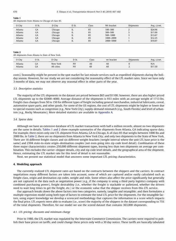
Table 1All shipments from Atlanta to Chicago of class 85.
O City O St. D City D St. Class Wt bracket Shipments Avg. c/cwt.
Atlanta GA Chicago IL 85 100–300 2 $24.96Atlanta GA Chicago IL 85 300–500 5 $17.09Atlanta GA Chicago IL 85 500–1000 3 $13.67Atlanta GA Chicago IL 85 1000–2000 1 $12.25Atlanta GA Chicago IL 85 2000–5000 1 $10.07
Table 2All shipments from Atlanta to State of New York.
O City O St. D City D St. Class wt bracket Shipments Avg. c/cwt.
Atlanta GA New York NY All All 0 N/AAtlanta GA All cities NY 60 All 2 $17.50
670 E. Özkaya et al. / Transportation Research Part E 46 (2010) 667–682
costs). Seasonality might be present in the spot market for last minute services such as expedited shipments during the holi-day season. However, for our study we are not considering the seasonality effect of the LTL market rates. Since we have only3 months of data, we may not observe any seasonal effect in other parts of the year.
3.3. Descriptive statistics
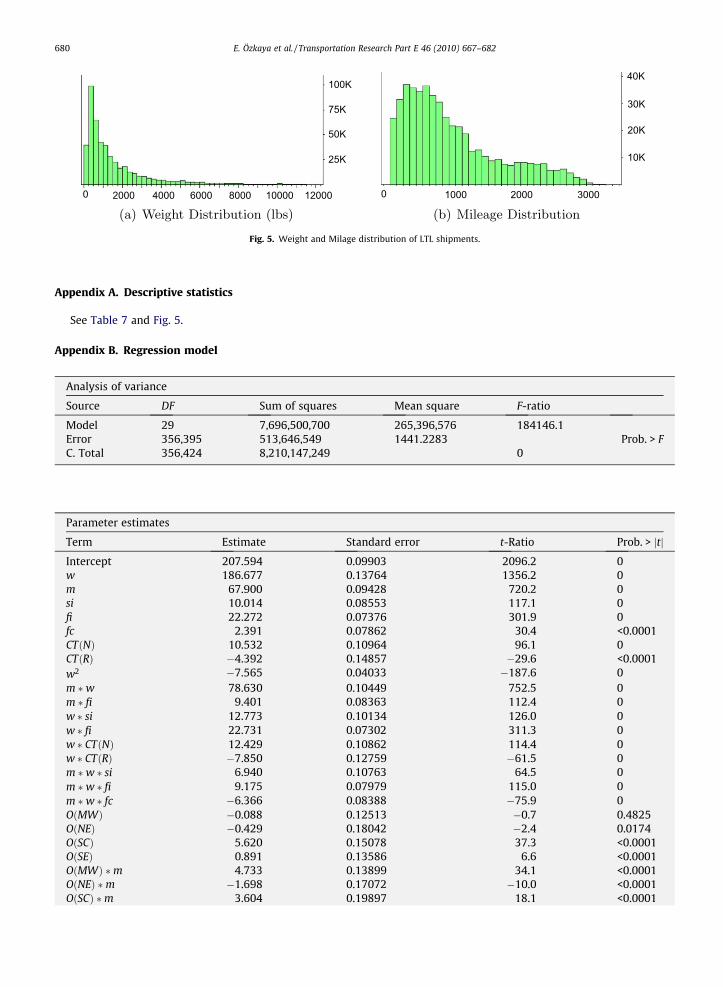
The majority of the LTL shipments in the dataset are priced between $65 and $1100; however, there are also higher pricedLTL shipments up to the $3000–4000. Average distance of the shipments is 933 miles with an average weight of 1713 lbs.Freight class changes from 50 to 150 for different types of freight including general merchandise, industrial lubricants, cereal,automotive spare parts, and other goods. For some of the US regions, the cost of LTL shipments might be higher or lower dueto special reasons such as congestion (e.g., New York City), supply-demand mismatch (e.g., South Florida) and level of urban-ism (e.g., Rocky Mountains). More detailed statistics are available in Appendix A.
3.4. Sparse data
Although we have an extensive database of LTL market transactions with half a million records, almost no two shipmentsare the same in details. Tables 1 and 2 show example summaries of the shipments from Atlanta, GA indicating sparse data.For example, there exists only one LTL shipment from Atlanta, GA to Chicago, IL of class 85 that weighs between 1000 lbs and2000 lbs. In Table 2, there are no shipments from Atlanta to New York City; and only two shipments to the State of New York.There are 18 different freight classes and six different weight-brackets (weight interval where the unit LTL base price is thesame) and 2304 state-to-state origin–destination couples (not even going into zip code level detail). Combination of thesethree major characteristics creates 250,000 different shipment types, leaving less than two shipments on average per com-bination. This excludes the carrier–shipper details, city and zip code level details, and the geographical area of the shipment.Hence, estimating the LTL market rate for this level of detail is not reasonable.
Next, we present our statistical model that uncovers some important LTL pricing characteristics.
4. Modeling approach
The currently realized LTL shipment rates are based on the contracts between the shippers and the carriers. In contractnegotiations many different factors are taken into account, some of which are captured and/or easily calculated such asfreight class, origin and destination zip codes, weight and mile. Some others also affect the price significantly but generallyare not captured in the data such as negotiation power (e.g., if the company is using a third party logistics company withcombined purchasing power), freight desirability (i.e., whether the freight is stackable or palletized, whether the driversneed to wait long times to get the freight, etc.) or the economic value that the shipper receives from this LTL service.
Our approach breaks down the above factors into two categories, namely, tangible and intangible; and then formulates amultiple regression model using both type of factors to estimate the total LTL price for the shipments. For the intangible fac-tors, using expert knowledge we develop a scorecard methodology that captures the information in a score which impactsthe final price. LTL experts were able to evaluate (i.e., score) the majority of the shippers in the dataset corresponding to 75%of the total shipments. Therefore, for our model we use the scored dataset that contains 363,000 shipments.
4.1. LTL pricing: discounts and minimum charge
Prior to 1980, the LTL market was regulated by the Interstate Commerce Commission. The carriers were required to pub-lish their base prices on tariffs, and could change these prices only with a 30 day notice. These tariffs are basically tabulated
E. Özkaya et al. / Transportation Research Part E 46 (2010) 667–682 671
market rates that give the base prices according to the freight’s origin–destination (O–D) zip codes, its freight class and itsweight. By forming rate bureaus, carriers established industry-wide tariffs. Because there was little incentive to changeprices due to regulation and limited competition, these tariffs became the de facto standard for LTL prices until 1980 (Baker,1991).
After the deregulation with the Motor Carrier Act of 1980, carriers started to offer discounts off of the published baseprices. These tariffs are now only a starting point for the negotiations. Many carriers changed (mostly increased) their baseprices so that they can offer better (higher) discounts to attract customers. Today, there are few industry-wide tariffs that arestill commonly used (i.e., Czarlite, Yellow 500); however there are total of 292 internal tariffs being used in the LTL Marketaccording to Material Handling Management online newsletter (Management, 2008). On top of the base prices, the followingdiscounts or changes can be applied to the price of LTL shipment as agreed by the carrier and the shipper.
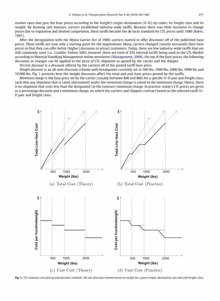
Percent discount is a discount offered by the carriers off of the posted tariff base price.Weight discount is an all-unit-discount scheme with breakpoints currently set at 500 lbs, 1000 lbs, 2000 lbs, 5000 lbs and
10,000 lbs. Fig. 1 presents how the weight discounts affect the total and unit base prices posted by the tariffs.Minimum charge is the base price set by the carrier (usually between $40 and $80) for a specific O–D pair and freight class,
such that any shipment that is rated (discounted) under the minimum charge is raised to the minimum charge. Hence, thereis no shipment that costs less than the designated (in the contract) minimum charge. In practice, today’s LTL prices are givenas a percentage discount and a minimum charge, on which the carriers and shippers contract based on the selected tariff, O–D pair and freight class.
Tota
l Lin
e H
aul C
ost
Weight (lbs)500 1000 2000
$ $To
tal L
ine
Hau
l Cos
t
Weight (lbs)500 1000 2000
Cos
t per
hun
dred
wei
ght
Weight (lbs)500 1000 2000
$
Weight (lbs)500 1000 2000
Cos
t per
hun
dred
wei
ght
$
Fig. 1. LTL Linehaul cost pricing and discount schedule. All unit discount scheme based on weight for a given origin–destination zip code and freight class.
672 E. Özkaya et al. / Transportation Research Part E 46 (2010) 667–682
In this research we focus on estimating the total price of the LTL shipments. Therefore our market rate estimates are inde-pendent of any tariff. Our aim is to create a model that will allow us to predict the market rate for any type of LTL shipmentwith high confidence given the origin–destination, freight class and weight. Desired minimum charges can then be applied ifthe market rate estimates are less than a certain minimum charge. Next, we present this holistic approach with multipleregression modeling.
4.2. Model
We propose a process and a model that estimates LTL market rates. Our prediction process has the following three steps:(1) Regionalization, (2) Multiple regression model, and (3) Post-regression analysis (optional).
Geographical regions impact the pricing of LTL services depending on the characteristics of the carriers operating withinthose regions and their different pricing policies. In our estimation process we first propose specific regions. Then we run ourmultiple regression model that consists of both tangible and intangible predictors together with origin and destination re-gion information. Finally we allow the users to bring their expertise into the analysis by considering other factors that maynot be captured by the general trend in the dataset. One such factor is the existence of flow imbalances for certain shipmentorigins or destinations. Hall (1999) analyzes a national LTL carrier network and finds that long run freight imbalances for thegiven network result in significant empty movement (i.e., dead miles) that is equal to 13.3% of the loaded movements ormore. This imbalance increases the cost of LTL carriers, and may affect the prices. Our dataset is limited to the shipmentsof a group of shippers and it does not contain all the shipments of any given LTL carrier. Therefore, it is hard to estimatethe level of imbalances for the given LTL carriers and deducing the effect of flow imbalances on LTL prices. A more completedataset of multiple carriers and their full set of shipments would be ideal for a future study to understand this effect in moredetail. Hall (1999) presents the relevant literature on the fleet management and equipment allocation problem. In a followup paper, Hall and Zhong (2002) analyze the simple management policies of empty equipment in the same LTL carrier’s net-work. While they do not analyze the effect of imbalances on the final price, they use cost of moving empty equipment, cost ofowning equipment and backorders as the performance metrics to evaluate policy decisions for balancing the network. Pool-ing multiple carriers, as in our analysis, minimizes ‘‘terminal specific” imbalances analyzed in Hall (1999); however, certainlocations, such as South Florida, can be an imbalance node for most carriers. In such situations, we leave the analysis to thepost-regression phase to determine the potential level of imbalance, and how that affects the pricing. Proposed regionaliza-tion step merely attempts to understand the differences in pricing practices of the carriers operating over these regions.
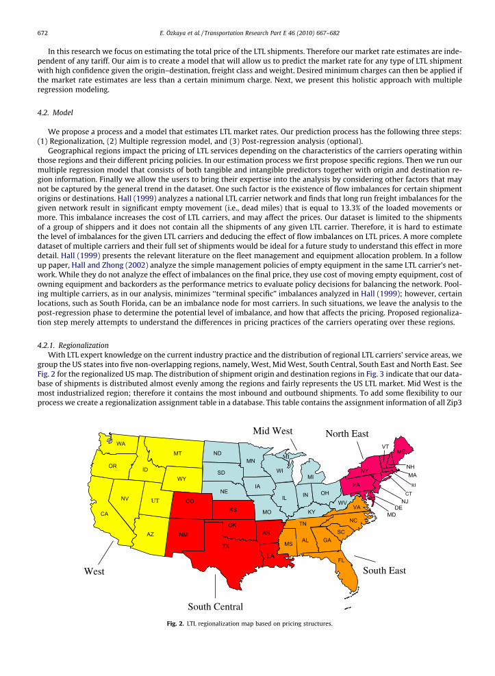
4.2.1. RegionalizationWith LTL expert knowledge on the current industry practice and the distribution of regional LTL carriers’ service areas, we
group the US states into five non-overlapping regions, namely, West, Mid West, South Central, South East and North East. SeeFig. 2 for the regionalized US map. The distribution of shipment origin and destination regions in Fig. 3 indicate that our data-base of shipments is distributed almost evenly among the regions and fairly represents the US LTL market. Mid West is themost industrialized region; therefore it contains the most inbound and outbound shipments. To add some flexibility to ourprocess we create a regionalization assignment table in a database. This table contains the assignment information of all Zip3
MT
WYID
WA
MS
OR
NV
CA
AZ
CO
NM
ND
NE
KS
OK
TX
MN
IA
MO
AR
WI
LA
AL
TN
KY
IL
MI
IN OH
NY
PA
GA
FL
NC
VA DEMD
NJ
NHMA
CT
ME
SC
WV
VT
SD
UT
MI
West
RI
South Central
South East
Mid West North East
Fig. 2. LTL regionalization map based on pricing structures.
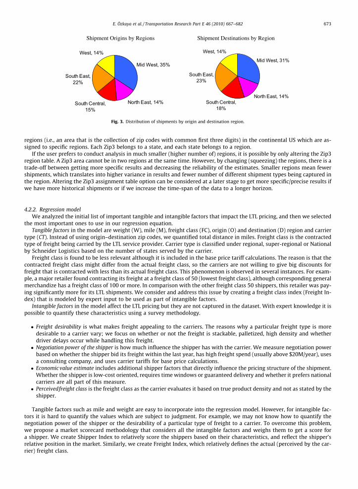
Shipment Destinations by RegionShipment Origins by Regions
Mid West, 35%
North East, 14%South Central, 15%
South East, 22%
West, 14%Mid West, 31%
North East, 14%South Central,
18%
West, 14%
South East, 23%
Fig. 3. Distribution of shipments by origin and destination region.
E. Özkaya et al. / Transportation Research Part E 46 (2010) 667–682 673
regions (i.e., an area that is the collection of zip codes with common first three digits) in the continental US which are as-signed to specific regions. Each Zip3 belongs to a state, and each state belongs to a region.
If the user prefers to conduct analysis in much smaller (higher number of) regions, it is possible by only altering the Zip3region table. A Zip3 area cannot be in two regions at the same time. However, by changing (squeezing) the regions, there is atrade-off between getting more specific results and decreasing the reliability of the estimates. Smaller regions mean fewershipments, which translates into higher variance in results and fewer number of different shipment types being captured inthe region. Altering the Zip3 assignment table option can be considered at a later stage to get more specific/precise results ifwe have more historical shipments or if we increase the time-span of the data to a longer horizon.
4.2.2. Regression modelWe analyzed the initial list of important tangible and intangible factors that impact the LTL pricing, and then we selected
the most important ones to use in our regression equation.Tangible factors in the model are weight (W), mile (M), freight class (FC), origin (O) and destination (D) region and carrier
type (CT). Instead of using origin–destination zip codes, we quantified total distance in miles. Freight class is the contractedtype of freight being carried by the LTL service provider. Carrier type is classified under regional, super-regional or Nationalby Schneider Logistics based on the number of states served by the carrier.
Freight class is found to be less relevant although it is included in the base price tariff calculations. The reason is that thecontracted freight class might differ from the actual freight class, so the carriers are not willing to give big discounts forfreight that is contracted with less than its actual freight class. This phenomenon is observed in several instances. For exam-ple, a major retailer found contracting its freight at a freight class of 50 (lowest freight class), although corresponding generalmerchandize has a freight class of 100 or more. In comparison with the other freight class 50 shippers, this retailer was pay-ing significantly more for its LTL shipments. We consider and address this issue by creating a freight class index (Freight In-dex) that is modeled by expert input to be used as part of intangible factors.
Intangible factors in the model affect the LTL pricing but they are not captured in the dataset. With expert knowledge it ispossible to quantify these characteristics using a survey methodology.
� Freight desirability is what makes freight appealing to the carriers. The reasons why a particular freight type is moredesirable to a carrier vary; we focus on whether or not the freight is stackable, palletized, high density and whetherdriver delays occur while handling this freight.� Negotiation power of the shipper is how much influence the shipper has with the carrier. We measure negotiation power
based on whether the shipper bid its freight within the last year, has high freight spend (usually above $20M/year), usesa consulting company, and uses carrier tariffs for base price calculations.� Economic value estimate includes additional shipper factors that directly influence the pricing structure of the shipment.
Whether the shipper is low-cost oriented, requires time windows or guaranteed delivery and whether it prefers nationalcarriers are all part of this measure.� Perceivedfreight class is the freight class as the carrier evaluates it based on true product density and not as stated by the
shipper.
Tangible factors such as mile and weight are easy to incorporate into the regression model. However, for intangible fac-tors it is hard to quantify the values which are subject to judgment. For example, we may not know how to quantify thenegotiation power of the shipper or the desirability of a particular type of freight to a carrier. To overcome this problem,we propose a market scorecard methodology that considers all the intangible factors and weighs them to get a score fora shipper. We create Shipper Index to relatively score the shippers based on their characteristics, and reflect the shipper’srelative position in the market. Similarly, we create Freight Index, which relatively defines the actual (perceived by the car-rier) freight class.

674 E. Özkaya et al. / Transportation Research Part E 46 (2010) 667–682
Shipper Index (SI) corresponds to a score between 0% and 100% and is calculated by answering the survey questions underthree major categories for each shipper, namely, freight desirability, negotiation power, and economic value estimate. Thehigher a shipper’s score, the higher is the LTL price that is likely to be charged for a similar shipment. These survey questionsare designed to be yes/no questions for simplicity, and they are answered by LTL experts for each shipper in the database.The purpose of the Shipper Index model is to create a standard framework to evaluate each shipper for characteristics thatare currently not captured with any data collection method, but play an important role in the negotiation process. By cre-ating a relative score for each shipper along the three dimensions mentioned, we intend to quantify the nontrivial aspects ofLTL pricing. Each category is presented with some questions targeted to analyze a different facet of that category. Some of thequestions have a positive impact on the price for the shipper, meaning that they ‘‘decrease” the LTL price, versus others havea negative impact. Table 3 shows the 12 yes/no questions (four for each category) presenting their relative weight (impor-tance level) within their category, their direction of impact (positive/negative) and the relative contribution of each categoryto the Shipper Index. The weights of the questions and the corresponding categories are discussed extensively and agreedupon with the LTL experts. In setting these parameters, we did not use the dataset in order to avoid over-fitting. We estab-lished a structure that we believe can be generalized to other industries. Test results show that our formulation of the Ship-per Index is a significant contributor to the regression model. While these parameters can be updated based on the changingmarket conditions, keeping yes/no type questions is an essential part of this model that helps eliminate subjective responsesto shipper characteristics.
Shipper Index is the weighted average of each category scores, and it is calculated as shown in Eq. (1),
Table 3Twelvecategor
Freig
Nego
Econ
SI ¼X
i
ciSi ð1Þ
where i is the category index, Si is the score of category i; ci is the weight of category i as listed in Table 3. With the currentcategory weights, Shipper Index is calculated as follows:
SI ¼ 0:6½Freight Desirability Score� þ 0:3½Negotiation Power Score� þ 0:1½Economic Value Estimate Score�
Each category score is calculated starting with its baseline and adding and subtracting the question weights that are an-swered ‘‘yes”. The positive question weights are subtracted as every positive action decreases the price, while the negativequestion weights are added to the baseline. Resulting category score is a discrete number as determined by the questionweights. Eq. (2) shows the category score calculations
Si ¼ Bi �Xj2Qiþ
wjyj þXj2Qi�
wjyj ð2Þ
where
Bi ¼Xj2Qiþ
wj; is the Baseline of category i
i ¼ Category index
j ¼ Question index
wj ¼Weight of Question j
yj ¼0; if the answer to question j is no
1; if the answer to question j is yes
�Q iþ ¼ Set of positive questions in category i
Q i� ¼ Set of negative questions in category i
yes/no questions within three categories used to calculate Shipper Index for each shipper. Weights of questions represents their importance within eachy.
ht desirability (60%) (+) Stackable freight? 20%(+) Palletized? 30%(+) High density? 20%(�) Driver delays? 30%
tiation power (30%) (+) Bid within last year? 40%(+) High freight spend? 10%(+) Using consulting company or 3PL? 20%(�) Using carrier tariffs? 30%
omic value estimate (10%) (+) Low cost? 60%(�) Time windows? 10%(�) Guaranteed delivery? 20%(�) Prefers Nat’l carriers over regional? 10%
E. Özkaya et al. / Transportation Research Part E 46 (2010) 667–682 675
With this type of formulation we allow relative scoring at two levels. The first one is at the category level. Each shipperhas a score that determines their category position. Then these category scores are weighted again at the higher level, whichconstitutes the Shipper Index and quantifies the currently non-captured information on each of the three categories.
Freight Index (FI) is the second component of the relative scoring mechanism and it aims to better inform our regressionmodel by understanding the contracting practices on the freight class and its relationship to the LTL base prices. With dataanalysis and industry expert knowledge we know that some shippers do not contract at their actual freight class, but try tocontract at a lower class. The main purpose of this is to lower the starting base price by lowering the freight class. Our anal-ysis shows that the shippers often do not benefit from reducing their freight class, since carriers do not compromise on thediscount levels in these situations. Therefore, we incorporate the actual (perceived) freight class into the intangible factors,specifically in the Freight Index that we calculate.
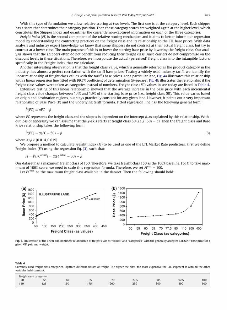
Another interesting observation is that the freight class value, which is generally referred as the product category in theindustry, has almost a perfect correlation with the tariff base prices. Testing a widely used industry tariff, we identify thelinear relationship of freight class values with the tariff’s base prices. For a particular lane, Fig. 4a illustrates this relationshipwith a linear regression line fitted with 99.7% coefficient of determination (R-square). Fig. 4b illustrates the relationship if thefreight class values were taken as categories instead of numbers. Freight class (FC) values in use today are listed in Table 4.
Extensive testing of this linear relationship showed that the average increase in the base price with each incrementalfreight class value changes between 1.4% and 1.9% of the starting base price (i.e., freight class 50). This value varies basedon origin and destination regions, but stays practically constant for any given lane. However, it points out a very importantrelationship of Base Price (P) and the underlying tariff formula. Fitted regression line has the following general form:
(a
Fig. 4.given O
Table 4Currentvariable
Freig50
110
bPðFCÞ ¼ aFC þ b
where FC represents the freight class and the slope a is dependent on the intercept b, as explained by this relationship. With-out loss of generality we can assume that the y-axis starts at freight class 50 (i.e.,bPð50Þ ¼ b). Then the freight class and BasePrice relationship takes the following form:
bPðFCÞ ¼ aðFC � 50Þ þ b ð3Þ
where a=b 2 ½0:014; 0:019�.We propose a method to calculate Freight Index (FI) to be used as one of the LTL Market Rate predictors. First we define
Freight Index (FI) using the regression Eq. (3), such that:
FI ¼ bPðFCactualÞ ¼ aðFCactual � 50Þ þ b
Our dataset has a maximum freight class of 150. Therefore, we take freight class 150 as the 100% baseline. For FI to take max-imum of 100% score, we need to scale this regression formula. Therefore, we set FImax ¼ 100.
Let FCmax be the maximum freight class available in the dataset. Then the following should hold:
R2 = 0.9972
0200400600800
1000120014001600
50 100 150 200 250 300 350 400 450
Freight Class (as values)
Bas
e P
rice
($) ILLUSTRATIVE LANE
0200400600800
1000120014001600
50 55 60 65 70 77.5 85 110 200 400
Freight Class (as categories)
Bas
e P
rice
($)
) (b)
Illustration of the linear and nonlinear relationship of freight class as ‘‘values” and ‘‘categories” with the generally accepted LTL tariff base price for aD pair and weight.
ly used freight class categories. Eighteen different classes of freight. The higher the class, the more expensive the LTL shipment is with all the others held constant.
ht class categories55 60 65 70 77.5 85 92.5 100
125 150 175 200 250 300 400 500
676 E. Özkaya et al. / Transportation Research Part E 46 (2010) 667–682
FImax ¼ bPðFCmaxÞ ¼ aðFCmax � 50Þ þ b ¼ 100
Since we do not know the actual distribution of a=b, we pick Mid West Region (that has the most inbound and outboundshipments) as the representative region. We find that a=b ¼ 0:017 is consistent for Mid West to Mid West shipments. Substi-tuting it to the above equation we find:
b� ¼ 100ð0:017ÞðFCmax � 50Þ þ 1
and a� ¼ 1:7ð0:017ÞðFCmax � 50Þ þ 1
Here scaled slope a� ensures that regression Eq. (3) gives a maximum value of 100. Using the linear relationship, we canre-write the Freight Index formula as in Eq. (4). Therefore, for a given actual (or perceived) freight class value, the FreightIndex is calculated as follows:
FI ¼ 100� a�ðFCmax � FCactualÞ ð4Þ
Modeling Freight Index this way helps us better predict the LTL market rates by better understanding the starting baseprices. Using the actual freight class to calculate the Freight Index further improves this relationship to the LTL market rate.Statistical results show that both Shipper Index and Freight Index are significant contributors of the final LTL price predic-tion. In fact, Freight Index is found to be much more significant than the original contracted freight class.
4.2.2.1. Multiple regression model. Shipper Index and Freight Index are both designed to relatively quantify each shipper’smarket position. Therefore, we create the following main predictors: Mile (M), Weight (W), Freight Class (FC), Shipper Index(SI), Freight Index (FI), Carrier Type (CT) , Origin region (O), and Destination region (D). To estimate the market rates of thespecific LTL shipment we propose the following general model:
y ¼ f ðM;W; FC; SI; FI; CT;O;DÞ þ e ð5Þ
where e is the random error due to other unobservable factors.After extensive model building and testing steps, we find that mile and weight are the most important factors. In addition,
we find their interaction effect ðM �WÞ and the quadratic effect of weight ðW2Þ to be significant. M and W are also found tointeract with the other factors. Therefore, we propose the following regression model:
y ¼ b0 þ b1M þ b2W þ b3M�W þ b4W2 þ e
where b0; b1; b2, and b3 are functions of the other predictors FC; SI; FI; CT; O, and D. However, b4 is taken as a constantbecause W2 has no interaction with the other factors. We use a linear predictor for each parameter bj. Thus, for eachj ¼ 0;1;2;3:
bj ¼ aj0 þ aj1FC þ aj2SI þ aj3CT½N� þ aj4CT½R� þ aj5O½MW� þ aj6O½NE� þ aj7O½SC� þ aj8O½SE� þ aj9D½MW� þ aj10D½NE�þ aj11D½SC� þ aj12D½SE�
Note that the carrier type predictor is replaced with two 0–1 dummy variables CT½N� and CT½R�, where CT½N� ¼ 1 when thecarrier type is National and 0 otherwise and CT½R� ¼ 1 when the carrier type is Regional and 0 otherwise. Similarly, four 0–1dummy variables are introduced for origin and destination regions, where MW, NE, SC, and SE stand for Mid West, North East,South Central, and South East regions, respectively. Thus, there are a total of 13 � 4 + 1 = 53 parameters in our regressionmodel. The actual relationship of LTL market rates with the suggested predictors can be nonlinear. However, the linear rela-tionship gives a good approximation for the given dataset except for the weight (W). In fact, a nonlinear relationship with Wis expected on theoretical grounds, see Fig. 1, due to the weight discount practices. We found that adding a quadratic term issufficient to capture the nonlinear relationship in the given dataset.
4.2.2.2. Standardizing the variables. Because the scales of the variables are quite different, we standardize the numerical pre-dictors such as Weight, Mile, Shipper Index, Freight Index, and Freight Class. This makes the relative comparison of the coef-ficients meaningful.
As a general rule, the predictor X is standardized as follows:
x ¼ X � Xsx
where X is the mean of the predictor X, sx is the standard deviation of X, and x is the standardized predictor. Table 5 providesthe means and standard deviations of standardized predictors for convenience.
One needs to standardize any shipment with the details listed in Table 5 to be able to use it in the regression model. Anyinteraction can be achieved by multiplying the corresponding standardized predictors.
4.2.2.3. Model selection. Since the initially proposed model contains 52 variables (and thus 53 parameters including theintercept), it is difficult to interpret and use in practice. Moreover, some of these variables may have practically insignificanteffects on the line haul price. Therefore, removing some of them will not adversely affect the prediction, but can help in sim-
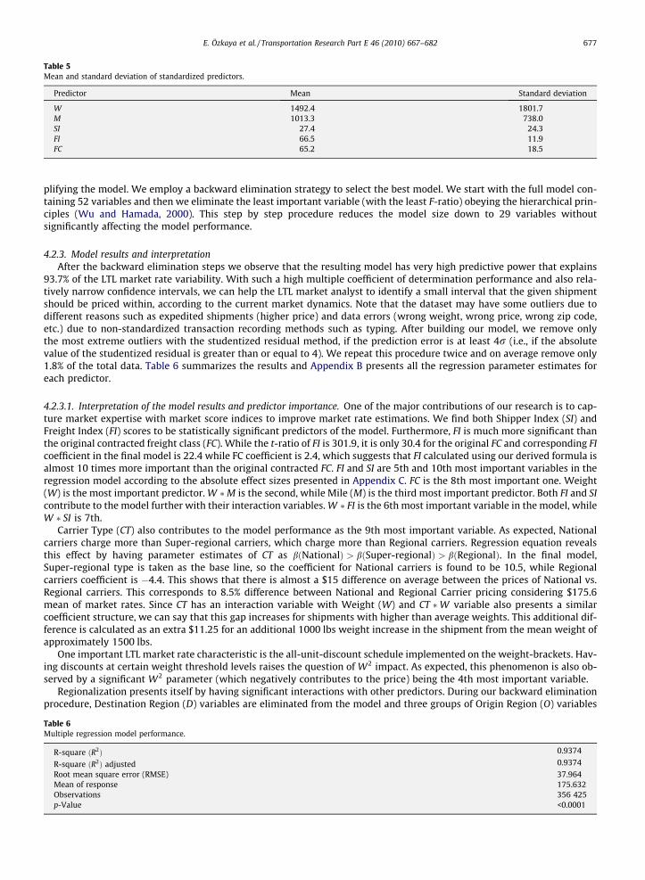
Table 5Mean and standard deviation of standardized predictors.
Predictor Mean Standard deviation
W 1492.4 1801.7M 1013.3 738.0SI 27.4 24.3FI 66.5 11.9FC 65.2 18.5
E. Özkaya et al. / Transportation Research Part E 46 (2010) 667–682 677
plifying the model. We employ a backward elimination strategy to select the best model. We start with the full model con-taining 52 variables and then we eliminate the least important variable (with the least F-ratio) obeying the hierarchical prin-ciples (Wu and Hamada, 2000). This step by step procedure reduces the model size down to 29 variables withoutsignificantly affecting the model performance.
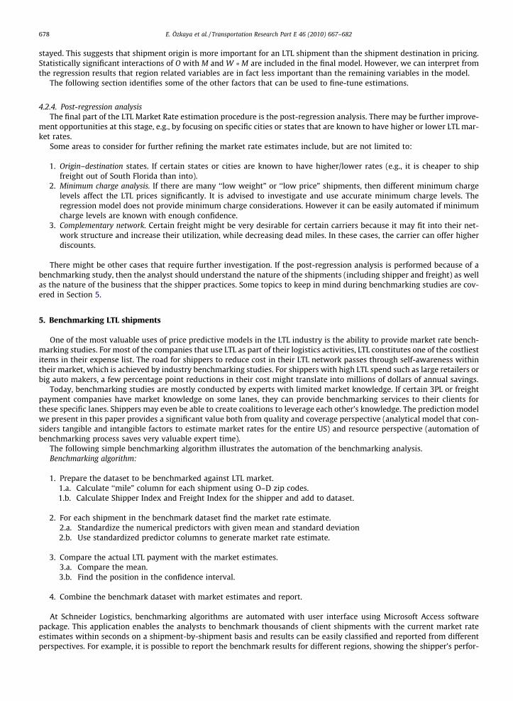
4.2.3. Model results and interpretationAfter the backward elimination steps we observe that the resulting model has very high predictive power that explains
93.7% of the LTL market rate variability. With such a high multiple coefficient of determination performance and also rela-tively narrow confidence intervals, we can help the LTL market analyst to identify a small interval that the given shipmentshould be priced within, according to the current market dynamics. Note that the dataset may have some outliers due todifferent reasons such as expedited shipments (higher price) and data errors (wrong weight, wrong price, wrong zip code,etc.) due to non-standardized transaction recording methods such as typing. After building our model, we remove onlythe most extreme outliers with the studentized residual method, if the prediction error is at least 4r (i.e., if the absolutevalue of the studentized residual is greater than or equal to 4). We repeat this procedure twice and on average remove only1.8% of the total data. Table 6 summarizes the results and Appendix B presents all the regression parameter estimates foreach predictor.
4.2.3.1. Interpretation of the model results and predictor importance. One of the major contributions of our research is to cap-ture market expertise with market score indices to improve market rate estimations. We find both Shipper Index (SI) andFreight Index (FI) scores to be statistically significant predictors of the model. Furthermore, FI is much more significant thanthe original contracted freight class (FC). While the t-ratio of FI is 301.9, it is only 30.4 for the original FC and corresponding FIcoefficient in the final model is 22.4 while FC coefficient is 2.4, which suggests that FI calculated using our derived formula isalmost 10 times more important than the original contracted FC. FI and SI are 5th and 10th most important variables in theregression model according to the absolute effect sizes presented in Appendix C. FC is the 8th most important one. Weight(W) is the most important predictor. W �M is the second, while Mile (M) is the third most important predictor. Both FI and SIcontribute to the model further with their interaction variables. W � FI is the 6th most important variable in the model, whileW � SI is 7th.
Carrier Type (CT) also contributes to the model performance as the 9th most important variable. As expected, Nationalcarriers charge more than Super-regional carriers, which charge more than Regional carriers. Regression equation revealsthis effect by having parameter estimates of CT as bðNationalÞ > bðSuper-regionalÞ > bðRegionalÞ. In the final model,Super-regional type is taken as the base line, so the coefficient for National carriers is found to be 10.5, while Regionalcarriers coefficient is �4.4. This shows that there is almost a $15 difference on average between the prices of National vs.Regional carriers. This corresponds to 8.5% difference between National and Regional Carrier pricing considering $175.6mean of market rates. Since CT has an interaction variable with Weight (W) and CT �W variable also presents a similarcoefficient structure, we can say that this gap increases for shipments with higher than average weights. This additional dif-ference is calculated as an extra $11.25 for an additional 1000 lbs weight increase in the shipment from the mean weight ofapproximately 1500 lbs.
One important LTL market rate characteristic is the all-unit-discount schedule implemented on the weight-brackets. Hav-ing discounts at certain weight threshold levels raises the question of W2 impact. As expected, this phenomenon is also ob-served by a significant W2 parameter (which negatively contributes to the price) being the 4th most important variable.
Regionalization presents itself by having significant interactions with other predictors. During our backward eliminationprocedure, Destination Region (D) variables are eliminated from the model and three groups of Origin Region (O) variables
Table 6Multiple regression model performance.
R-square ðR2Þ 0.9374
R-square ðR2Þ adjusted 0.9374
Root mean square error (RMSE) 37.964Mean of response 175.632Observations 356 425p-Value <0.0001
678 E. Özkaya et al. / Transportation Research Part E 46 (2010) 667–682
stayed. This suggests that shipment origin is more important for an LTL shipment than the shipment destination in pricing.Statistically significant interactions of O with M and W �M are included in the final model. However, we can interpret fromthe regression results that region related variables are in fact less important than the remaining variables in the model.
The following section identifies some of the other factors that can be used to fine-tune estimations.
4.2.4. Post-regression analysisThe final part of the LTL Market Rate estimation procedure is the post-regression analysis. There may be further improve-
ment opportunities at this stage, e.g., by focusing on specific cities or states that are known to have higher or lower LTL mar-ket rates.
Some areas to consider for further refining the market rate estimates include, but are not limited to:
1. Origin–destination states. If certain states or cities are known to have higher/lower rates (e.g., it is cheaper to shipfreight out of South Florida than into).
2. Minimum charge analysis. If there are many ‘‘low weight” or ‘‘low price” shipments, then different minimum chargelevels affect the LTL prices significantly. It is advised to investigate and use accurate minimum charge levels. Theregression model does not provide minimum charge considerations. However it can be easily automated if minimumcharge levels are known with enough confidence.
3. Complementary network. Certain freight might be very desirable for certain carriers because it may fit into their net-work structure and increase their utilization, while decreasing dead miles. In these cases, the carrier can offer higherdiscounts.
There might be other cases that require further investigation. If the post-regression analysis is performed because of abenchmarking study, then the analyst should understand the nature of the shipments (including shipper and freight) as wellas the nature of the business that the shipper practices. Some topics to keep in mind during benchmarking studies are cov-ered in Section 5.
5. Benchmarking LTL shipments
One of the most valuable uses of price predictive models in the LTL industry is the ability to provide market rate bench-marking studies. For most of the companies that use LTL as part of their logistics activities, LTL constitutes one of the costliestitems in their expense list. The road for shippers to reduce cost in their LTL network passes through self-awareness withintheir market, which is achieved by industry benchmarking studies. For shippers with high LTL spend such as large retailers orbig auto makers, a few percentage point reductions in their cost might translate into millions of dollars of annual savings.
Today, benchmarking studies are mostly conducted by experts with limited market knowledge. If certain 3PL or freightpayment companies have market knowledge on some lanes, they can provide benchmarking services to their clients forthese specific lanes. Shippers may even be able to create coalitions to leverage each other’s knowledge. The prediction modelwe present in this paper provides a significant value both from quality and coverage perspective (analytical model that con-siders tangible and intangible factors to estimate market rates for the entire US) and resource perspective (automation ofbenchmarking process saves very valuable expert time).
The following simple benchmarking algorithm illustrates the automation of the benchmarking analysis.Benchmarking algorithm:
1. Prepare the dataset to be benchmarked against LTL market.1.a. Calculate ‘‘mile” column for each shipment using O–D zip codes.1.b. Calculate Shipper Index and Freight Index for the shipper and add to dataset.
2. For each shipment in the benchmark dataset find the market rate estimate.2.a. Standardize the numerical predictors with given mean and standard deviation2.b. Use standardized predictor columns to generate market rate estimate.
3. Compare the actual LTL payment with the market estimates.3.a. Compare the mean.3.b. Find the position in the confidence interval.
4. Combine the benchmark dataset with market estimates and report.
At Schneider Logistics, benchmarking algorithms are automated with user interface using Microsoft Access softwarepackage. This application enables the analysts to benchmark thousands of client shipments with the current market rateestimates within seconds on a shipment-by-shipment basis and results can be easily classified and reported from differentperspectives. For example, it is possible to report the benchmark results for different regions, showing the shipper’s perfor-
E. Özkaya et al. / Transportation Research Part E 46 (2010) 667–682 679
mance with respect to a market for similar freight. A shipper therefore can see which regions to focus on for cost savings.Another reporting can be done across the same industry. If the market data includes other companies within the same indus-try, then clients can see their position within this market. Benchmarks can also show the purchasing effectiveness of 3PLcompanies by comparing their current customers with other companies, therefore showing the extra potential cost savingsfor 3PL’s customers.
Shipment level benchmark studies enable analysts to provide tailored and specific benchmarks of interest. Combinedwith estimation models, benchmarking algorithms are clearly a market visibility tool. They can be used to research marketdynamics/trends over time, to find market areas for developing successful new product offerings, and to enable greater nego-tiation leverage for both shippers and carriers.
6. Conclusion
The primary contribution of this study is the understanding of the main drivers in LTL pricing structure by analyzing aunique industry dataset consisting of shipments from a wide range of shippers and carriers. We contribute to the literatureby analyzing transactional/shipment-level data and providing a methodology to capture expert knowledge on some of thekey drivers of LTL pricing. This approach brings to light some LTL practices, such as negotiations and contracting, that arepreviously not investigated with analytical modeling. We propose a regression based estimation model that explains signif-icant majority of the LTL market rate variability. We consider both tangible and intangible factors in our model. We provide ascorecard methodology to objectively quantify the intangible factors that are important to LTL pricing, yet not captured inany dataset. There are two major findings from this study. First, the intangible factors such as freight desirability, negotiationpower and economic value estimate are found to be significant contributors to the LTL market rates. Therefore, shipperswhose freight is less desirable to carriers, who do not have much negotiation power, and who receive great economic benefitfrom the LTL service should expect to pay higher prices for a shipment than a shipper with opposite characteristics eventhough the freight class, the weight of the freight, and the lanes may be the same. Second, the shippers who try to contractfor a lower freight class than their actual freight in order to lower the base prices (i.e., starting point of the negotiations), donot often realize the expected benefit of a lower base price. Actual freight class as perceived by the carrier is found to be amuch more significant predictor of final LTL prices than the contracted freight class.
Overall, the ability to easily estimate and benchmark LTL market rates is a very beneficial market visibility tool that allowsanalysts to do extensive research on the LTL market. For 3PL companies, it can be a revenue source for consulting services.Also it can be used as the source for accurate market rates for network design studies. For carriers, the market knowledgebrings a serious competitive advantage. Knowing the main drivers of LTL market pricing, carriers might benefit in pricingtheir own services or offering new services that can be successful in the market. For shipper companies, this tool can improvemarket visibility and help to realize their market performance, potentially leading the way to extensive cost savings. Evenwithout owning the extensive LTL market data, most up-to-date regression models can serve the shipper needs.
One of the most beneficial areas to apply our predictive model is in benchmarking studies. Benchmarking algorithms pro-vide additional value to the prediction models. They enable analysts to benchmark any company’s historical LTL shipmentswith the same-dated market data. Automation of these models and algorithms makes the process of market research muchfaster. This creates an opportunity to reduce the cycle time of benchmarking studies, decreasing the time required from ex-perts and making it possible to serve many potential clients with consulting services.
Acknowledgments
We would like to thank Schneider Logistics’ LTL industry experts Helge Tangen and Chris Renier for their tremendous sup-port and contributions to our paper. Authors also would like to thank Dr. Paul Kvam of H. Milton Stewart School of Industrialand Systems Engineering for his guidance and comments to improve our models. This research is supported in part by NSFGrant SBE-0624269.
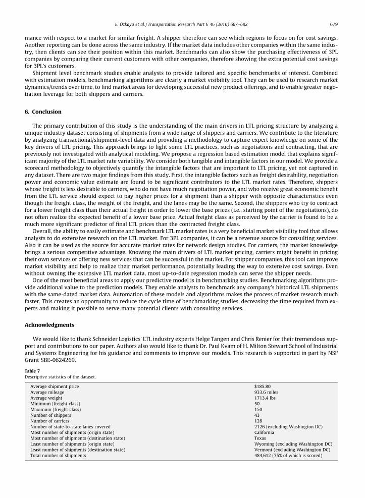
Table 7Descriptive statistics of the dataset.
Average shipment price $185.80Average mileage 933.6 milesAverage weight 1713.4 lbsMinimum (freight class) 50Maximum (freight class) 150Number of shippers 43Number of carriers 128Number of state-to-state lanes covered 2126 (excluding Washington DC)Most number of shipments (origin state) CaliforniaMost number of shipments (destination state) TexasLeast number of shipments (origin state) Wyoming (excluding Washington DC)Least number of shipments (destination state) Vermont (excluding Washington DC)Total number of shipments 484,612 (75% of which is scored)
2000 4000 6000 8000 10000 12000
25K
75K
100K
0
50K
10000 2000 3000
10K
30K
20K
40K
Fig. 5. Weight and Milage distribution of LTL shipments.
680 E. Özkaya et al. / Transportation Research Part E 46 (2010) 667–682
Appendix A. Descriptive statistics
See Table 7 and Fig. 5.
Appendix B. Regression model
Analysis of variance
Source
DF Sum of squares Mean square F-ratioModel
29 7,696,500,700 265,396,576 184146.1 Error 356,395 513,646,549 1441.2283 Prob. > F C. Total 356,424 8,210,147,249 0Parameter estimates
Term
Estimate Standard error t-Ratio Prob. > jtjIntercept
207.594 0.09903 2096.2 0 w 186.677 0.13764 1356.2 0 m 67.900 0.09428 720.2 0 si 10.014 0.08553 117.1 0 fi 22.272 0.07376 301.9 0 fc 2.391 0.07862 30.4 <0.0001 CTðNÞ 10.532 0.10964 96.1 0 CTðRÞ �4.392 0.14857 �29.6 <0.0001 w2 �7.565 0.04033 �187.6 0 m �w 78.630 0.10449 752.5 0 m � fi 9.401 0.08363 112.4 0 w � si 12.773 0.10134 126.0 0 w � fi 22.731 0.07302 311.3 0 w � CTðNÞ 12.429 0.10862 114.4 0 w � CTðRÞ �7.850 0.12759 �61.5 0 m �w � si 6.940 0.10763 64.5 0 m �w � fi 9.175 0.07979 115.0 0 m �w � fc �6.366 0.08388 �75.9 0 OðMWÞ �0.088 0.12513 �0.7 0.4825 OðNEÞ �0.429 0.18042 �2.4 0.0174 OðSCÞ 5.620 0.15078 37.3 <0.0001 OðSEÞ 0.891 0.13586 6.6 <0.0001 OðMWÞ �m 4.733 0.13899 34.1 <0.0001 OðNEÞ �m �1.698 0.17072 �10.0 <0.0001 OðSCÞ �m 3.604 0.19897 18.1 <0.0001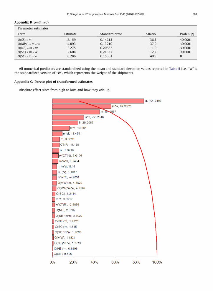
E. Özkaya et al. / Transportation Research Part E 46 (2010) 667–682 681
Appendix B (continued)
Parameter estimates
Term
Estimate Standard error t-Ratio Prob. > jtjOðSEÞ �m
5.159 0.14213 36.3 <0.0001 OðMWÞ �m �w 4.893 0.13210 37.0 <0.0001 OðNEÞ �m �w �2.275 0.20682 �11.0 <0.0001 OðSCÞ �m �w 2.604 0.21337 12.2 <0.0001 OðSEÞ �m �w 6.286 0.15361 40.9 0All numerical predictors are standardized using the mean and standard deviation values reported in Table 5 (i.e., ‘‘w” isthe standardized version of ‘‘W”, which represents the weight of the shipment).
Appendix C. Pareto plot of transformed estimates
Absolute effect sizes from high to low, and how they add up.

682 E. Özkaya et al. / Transportation Research Part E 46 (2010) 667–682
References
Baker, J., 1991. Emergent pricing structures in LTL transportation. Journal of Business Logistics 12, 191–202.Barnhart, C., Kim, D., 1995. Routing models and solution procedures for regional Less-than-Truckload operations. Annals of Operations Research 61, 67–90.Barrett, C., 2007. Discounts are Legitimate, But Beware, Traffic World, 38, July 2.Bohman, R., 2007. STB Hands Down Major Trucking Deregulation Decision. Logistics Management, June 1. <http://www.logisticsmgmt.com/article/
CA6451283.html>.Carter, J., Ferrin, B., Carter, C., 1995. The effect of Less-than-Truckload rates on the purchase order lot size decision. Transportation Journal 34, 35–44.Centa, H., 2007. Facts On Freight – What Determines LTL Discount Percentages, Production Machining, 20–21, December 1.Chainalytics, L., 2008. Model-Based Benchmarking Consortium. <http://www.chainalytics.com/services/transport_mbbc.asp>.Chiang, Y.S., Roberts, P.O., 1980. A note on transit time and reliability for regular-route trucking. Transportation Research Part B: Methodological 14 (March–
June), 59–65.Chu, C.W., 2005. A heuristic algorithm for the truckload and Less-than-Truckload problem. European Journal of Operational Research 165, 657–667.CSCMP, 2007. 19th Annual State of Logistics Report, CSCMP.org.Elmaghraby, W., Keskinocak, P., 2003. Combinatorial auctions in procurement. In: Billington, C., Harrison, T., Lee, H., Neale, J. (Eds.), The Practice of Supply
Chain Management. Kluwer Academic Publishers.Grant, K.B., Kent, J.L., 2006. Investigation of Methodologies Used by Less-than-Truckload (LTL) Motor Carriers to Determine Fuel Surcharges. Technical
Report by Midwest Transportation Consortium, MTC Project 2006-03.Hall, R., 1999. Stochastic freight flow patterns: implications for fleet optimization. Transportation Research Part A: Policy and Practice 33, 449–465.Hall, R.W., Zhong, H., 2002. Decentralized inventory control policies for equipment management in a many-to-many network. Transportation Research Part
A: Policy and Practice 36 (December), 849–865.Hannon, D., 2006a. Best-kept secrets for reducing LTL costs. Purchasing (May), 33–36.Hannon, D., 2006b. LTL buyers face an uphill battle. Purchasing (April), 42.Katayama, N., Yurimoto, S., 2002. The Load Planning Problem for Less-than-Truckload Motor Carriers and Solution Approach. Working Paper, Ryutsu Keizai
University, Ibaraki, Japan.Keaton, M.H., 1993. Are there economies of traffic density in the Less-than-Truckload motor carrier industry? An operations planning analysis.
Transportation Research Part A: Policy and Practice 27 (September), 343–358.Management, M.H., 2008. Tariff Practices Add Complexity For Carriers. Material Handling Management Online. <http://www.mhmonline.com/nID/2252/
MHM/viewStory.asp>.Murphy, P., Corsi, T., 1989. Modelling sales force turnover among LTL motor carriers: a management perspective. Transportation Journal 19, 25–37.
September 1.Schulz, J.D., 2007. LTL Market Update: Getting the balance right. Logistics Management, June 1. <http://www.logisticsmgmt.com/article/CA6451284.html>.Smith, L., Campbell, J., Mundy, R., 2007. Modeling net rates for expedited freight services. Transportation Research Part E: Logistics and Transportation
Review 43, 192–207.Spady, R., Friedlaender, A., 1978. Hedonic cost functions for the regulated trucking industry. The Bell Journal of Economics 9, 159–179.Winston, C., Corsi, T., Grimm, C., Evans, C., 1990. The Economic Effects of Surface Freight Deregulation. Brookings Institution Press.Wu, C.F.J., Hamada, M., 2000. Experiments: Planning, Analysis, and Parameter Design Optimization. Wiley, New York.