estimating a dynamic factor model in eviews using …1091335/fulltext02.pdfestimating a dynamic...
TRANSCRIPT

Working Paper 2017:2
Department of Statistics
Estimating a dynamic
factor model in EViews
using the Kalman Filter
and smoother
Martin Solberger & Erik Spånberg

Working Paper 2017:2
April 2017
Department of Statistics
Uppsala University
Box 513
SE-751 20 UPPSALA
SWEDEN
Working papers can be downloaded from www.statistics.uu.se
TITLE: Estimating a dynamic factor model in EViews using the Kalman Filter and smoother
AUTHOR: Martin Solberger & Erik Spånberg
E-MAIL: [email protected]

Estimating a Dynamic Factor Model in EViewsUsing the Kalman Filter and Smoother
Martin SolbergerUppsala University
Ministry of Finance, Sweden
Erik SpanbergMinistry of Finance, Sweden
Abstract
In this paper, we set up a dynamic factor model in EViews using only a small amountof programming. The model is particularly useful for nowcasting the economy, that is,forecasting of the very recent past, the present, or the very near future of economic activity.A subroutine that estimates the model is provided. In a simulation study, the precisionof the estimated factors are evaluated, and in an empirical example, the usefulness of themodel is illustrated.
Keywords: dynamic factor model, state space, kalman filter, EViews.
1. Introduction
Factor models are used in data-rich environments. The basic idea is to separate a possiblylarge number of observable variables into two independent and unobservable, yet estimable,components: a ’common component’ that captures the main bulk of co-movement between theobservable variables, and an ’idiosyncratic component’ that captures any remaining individualmovement. The common component is assumed to be driven by a few common factors, therebyreducing the dimension of the system. Whereas early contributions assume independent andidentically distributed (i.i.d.) random variables, subsequent research, mainly within signalprocessing and macroeconometrics, have developed the notion of dynamic factor models,modeling dependent time series variables.
In Economics, dynamic factor models are motivated by theory, which predicts that macroe-conomic shocks should be pervasive and affect most variables within an economic system.They have therefore become popular among macroeconometricians (see, e.g., Breitung andEickmeier 2006, for an overview). In particular, it has been demonstrated that dynamic factormodels are valuable in business cycle analysis (e.g. Forni and Reichlin 1998; Eickmeier 2007;Ritschl, Sarferaz, and Uebele 2016), forecasting (e.g. Stock and Watson 2002a,b) and now-casting the state of the economy, that is, forecasting of the very recent past, the present, orthe very near future of indicators for economic activity, such as the Gross Domestic Product(GDP) (see, e.g., Banbura, Giannone, Modugno, and Reichlin 2012, and references therein).Information of the economic activity is of great importance for decision makers in, for instance,governments, central banks and financial markets. However, first official estimates of GDP arepublished with a significant delay, usually about 6-8 weeks after the reference quarter, whichmakes nowcasting very useful. Other areas of economic analysis using dynamic factor models

2 EViews: Estimating a Dynamic Factor Model
include, for example, yield curve modeling (e.g. Diebold and Li 2006; Diebold, Rudebusch,and Aruoba 2006), financial risk-return analysis (Ludvigson and Ng 2007), and monetarypolicy analysis (e.g. Bernanke, Boivin, and Eliasz 2005; Boivin, Giannoni, and Mihov 2009).Despite the attractiveness of dynamic factor models for macroeconomists, econometric or sta-tistical softwares do not in general provide these models within standard packages. In thispaper, we illustrate how to, by means of simple programming, set up the popular two-stepestimator of Doz, Giannone, and Reichlin (2011) in EViews (IHS Global Inc. 2015a,b,c,d),a statistical software specialized in time series analysis that is broadly used by economists,econometricians, and statisticians.
The parameters of dynamic factor models can be estimated by the method of principal com-ponents. This method is easy to compute, and is consistent under quite general assumptionsas long as both the cross-section and time dimension grow large. It suffers, however, from alarge drawback: the data set must be balanced, where the start and end points of the sampleare the same across all observable variables. In practice, data are often released at differentdates. A popular approach is therefore to cast the dynamic factor model in a state space rep-resentation and then estimate it using the Kalman filter, which allows unbalanced data setsand offers the possibility to smooth missing values. The state space representation containsa signal equation, which links observed variables to latent states, and a state equation, whichdescribes how the states evolve over time. The Kalman filter and smoother provide mean-square optimal projections for both the signal and state variables. The method we set upin this paper uses the principal components estimates to re-estimate the factors decomposedas the latent states using the Kalman filter and smoother. We provide a subroutine for thismethod, which is evaluated in a simulation study and applied in an empirical example. Allcoding was done in EViews 9.5.
The rest of the paper is organized as follows. Section 2 describes the properties of dynamicfactor models and conventional estimation procedures. Section 3 derives a state space solu-tion. Section 4 goes through the specific method of estimation used in this paper. Section 5evaluates the method of estimation by means of simulation. Section 6 provides an empiricalexample. Section 7 concludes. Complete codes are placed in appendices: A subroutine withthe method of estimation is provided in Appendix A, and the code used for the simulationstudy is provided in Appendix B.
Some remarks on notation: We let In denote the n × n identity matrix. For any squarematrix A ∈ Rn×n, ϕ1(A) ≥ ϕ2(A) ≥ · · · ≥ ϕn(A) denote the ordered eigenvalues, andA = diag (a1, a2, . . . , an) states that A is a diagonal matrix with entries a1, a2, . . . , an on itsmain diagonal. For any matrix A ∈ Rn×m, ||A|| = [tr(AA′)]1/2 denotes the Frobenius norm,and A = [ai,j ]n×m states that A has elements ai,j corresponding to the ith row and jthcolumn (i = 1, 2, ..., n; j = 1, 2, ...,m). We let N denote the normal distribution and U denotethe uniform distribution. For a panel, N and T denote the cross-section and time dimension,respectively, N → denotes the limit taken over N , and N,T → denotes the joint limit takenover T and N simultaneously. We use
p→ to denote convergence in probability.
2. A dynamic factor model
Let xt = (x1,t, x2,t, ..., xN,t)′ be a vector of N time series, and let the empirical information
available at time t (t = 1, 2, ..., T ) be condensed into the information set Ft = x1,x2, ...,xt.

Martin Solberger, Erik Spanberg 3
A dynamic factor model is usually specified such that each observable xi,t (i = 1, 2, ..., N)is the sum of two independent and unobservable components: a common component χi,t,which is driven by a small number of factors that are common to all individuals, and aremaining idiosyncratic (individual-specific) component εi,t (see, e.g., Bai and Ng 2008). Inpanel notation, the model is
xi,t = χi,t + εi,t, (i = 1, 2, ..., N ; t = 1, 2, ..., T ), (1)
χi,t = υi(L)′zt,
where υi(L) = υi,0 + υi,1L + · · · + υi,κL` is a vector lag-polynomial, possibly of infinite
order, loading onto a vector of K unobservable common factors, zt = (z1,t, z2,t, ..., zK,t)′.1
Thus, only the left-hand side of Equation (1) is observed; the right-hand side is unobserved.If the dimension of zt is finite (K < ∞), then there exists for every i an R × 1 vector(R ≥ K) of constants λi = (λi,1, λi,2, ..., λi,R)′, such that υi(L)′ = λ′iC(L), where C(L) isan R × K matrix lag-polynomial, of infinite order in general, C(L) =
∑∞m=0 CmL
m, that isabsolutely summable,
∑∞m=0 ||Cm|| < ∞ (see Forni, Giannone, Lippi, and Reichlin 2009).
Thus, letting ft = (f1,t, f2,t, ..., fR,t)′ = C(L)zt, the dynamic factor model can be cast in the
static representation
xi,t = ci,t + εi,t, (2)
ci,t = λ′ift,
which, equivalently, can be written in vector notation as
xt = ct + εt, (3)
ct = Λft,
where ct = (c1,t, c2,t, ..., cN,t)′, εt = (ε1,t, ε2,t, ..., εN,t)
′ and Λ = (λ′1,λ′2, ...,λ
′N )′. The common
factors in zt are often referred to as dynamic factors, while the common factors in ft arereferred to as static factors. The number of static factors, R, cannot be smaller than thenumber of dynamic factors, and is typically much smaller than the number of cross-sectionalindividuals, K ≤ R N . As with χi,t in the dynamic representation (1), we refer to thescalar process ci in (2), or the multivariate process ct in (3), as the common component.
In general, we suppose that every xi,t is a weakly stationary process with mean zero thathas, at least, finite second-order moments, E(xi,t) = 0, E(xi,txi,t−s) < ∞ (s = 0, 1, 2, ...). Touphold this, something close to the following is usually assumed:
A1 (common factors) The q-variate process zt is orthonormal white noise, that is, indepen-dent and identically distributed (i.i.d.) over both the cross-section and time dimensionwith zero mean: E(zt) = 0,E(ztz
′t) = diag(ω2
1, ω22, ..., ω
2R), where ω2
j < ∞ for all j, andE(ztz
′s) = 0 for all t 6= s.
A2 (idiosyncratic components) The univariate process εi,t admits the Wold representationεi,t = θi(L)ui,t =
∑∞m=0 θi,mui,t−m, where
∑∞m=0 |θi,m| <∞ and ui,t is i.i.d. white noise
with limited cross-sectional dependence: E(ui,t) = 0, E(ui,tuj,s) = 0 for all t 6= s, and
E(ui,tuj,t) = τi,j , with∑N
i=0 |τi,j | < J , where J is some positive number that does notdepend on N or T .
1Here, the lag transpose is defined as υi(L)′ = υ′i,1L+ υ′i,2L2 + · · ·+ υ′i,`L
`, where, for q = 1, 2, ..., `, υi,qare K × 1 vectors, such that χi,t = υ′i,0zt + υ′i,1zt−1 + · · ·+ υ′i,κzt−`.

4 EViews: Estimating a Dynamic Factor Model
A3 (independence) The common shocks zt and idiosyncratic errors ut = (ui,t, u2,t, ..., uN,t)′,
are mutually independent groups, E(utz′s) = 0 for all t, s.
From Assumption A1, the static factors are stationary and variance-ergodic processes admit-ting a Wold representation ft = C(L)zt =
∑∞m=0 Cmzt−m. Assuming invertibility, the static
factors may therefore follow some stationary VAR(p) process,
A(L)ft = zt, (4)
where A(L) = IR −A1L−A2L2 − · · · −ApL
p = C(L)−1.
We have assumed here, for the sake of argument, that the dynamic factors zt (sometimesreferred to as the primitive shocks) enters as errors in the static factor VAR process (4). Thisis unnecessarily strict. To be more precise, by suitably defining ft, the dynamic factor model(1) can in general be cast in the static representation (2), where ft follows a VAR processwhich exact order depends on the specific dynamics of zt. The number of static factors isalways R = K(`+1); see Bai and Ng (2007). In practice, the static representation is typicallystated without reference to a more general dynamic factor model. Additionally, it is oftenassumed that the static common factors follow a stationary VAR process. Assumption A1 isinnocuous, as we may assume that zt is an orthonormal error of the static factor VAR process,and that this, in general, relates to some dynamic factor model (1).
Now, from Assumptions A1-A3, the autocovariance of the panel data is
Γx(h) = E(xtx′t−h) = ΛΓf (h)Λ′ + Γε(h), (5)
where Γf (h) = E(ftf′t−h) and Γε(h) = E(εtε
′t−h). By denoting Σ = Γx(0), Υ = Γf (0) and
Ψ = Γε(0), we can write the contemporary covariance matrix of xt as Σ = ΛΥΛ′ + Ψ. Thiscovariance matrix is of central importance for dynamic factor models. If the largest eigen-value of Ψ is bounded as N → ∞, then we have an approximate factor model as defined byChamberlain and Rothschild (1983). Approximate factor models have become very popularwithin, for instance, panel data econometrics, because they allow for a cross-sectional depen-dence among εt, whilst letting the factor structure be identified. If Ψ is diagonal, then wehave the exact (or strict) factor model. Since the diagonal elements of Ψ are real and finite,the exact factor model is nested within the approximate factor model as a special case. Thelargest eigenvalue of Ψ is, in fact, smaller than maxj
∑Ni=1 |E(εi,tεj,t)| (see Bai 2003), which is
bounded with respect to both N and T by Assumption A2.2 Hence, by assumption, we havean approximate factor model.
On top of this, some technical requirements are usually placed on the factor loadings, suchthat the common component is pervasive as the number of cross-sectional individuals increase.In essence, as N →∞, all eigenvalues of N−1Λ′Λ should be positive and finite, implying thatthe R largest eigenvalues of Σ are unbounded asymptotically.3
2From Assumption A2, E(εi,tεj,t) =∑∞m=0 θi,mE(ui,t−muj,t−m) =
∑∞m=0 θi,mτi,j = τi,j
∑∞m=0 θi,m. Thus,
|E(εi,tεj,t)| = |τi,j ||∑∞m=0 θi,m|, and so maxj
∑Ni=1 |E(εi,tεj,t)| = |
∑∞m=0 θi,m|maxj
∑Ni=1 |τi,j | <∞.
3By construction, theR×R matrix Λ′Λ is positive definite, whereas the N×N matrix ΛΛ′ is positive semi-definite. It is easily established (see, e.g., Zhou and Solberger 2017, Lemma A1) that the (positive) eigenvaluesof Λ′Λ correspond exactly to the non-zero eigenvalues of ΛΛ′. That is, for i = 1, 2, ...,R, ϕi(ΛΛ′) = ϕi(Λ
′Λ),while for i = R+1,R+2, ..., N , ϕi(ΛΛ′) = 0. Because the eigenvalues of N−1Λ′Λ are non-zero, the eigenvaluesof ΛΛ′ are unbounded as N →∞.

Martin Solberger, Erik Spanberg 5
Note finally that, unless we impose restrictions, the factors and factor loadings are onlyidentified up to pre-multiplication with an arbitrary R × R full rank matrix M. That is,Equation (3) is observationally equivalent to xt = Λ0f0t +εt where Λ0 = ΛM and f0t = M−1ft.Likewise, in terms of variances, we have that Σ = ΛΥΛ′+Ψ = ΛMM−1E(ftft)
′M′−1M′Λ′ =ΛME(M−1ftf
′tM′−1)M′Λ′ + Ψ = Λ0VAR(f0t )Λ0′ + Ψ. Due to this rotational indeterminacy,
we may without loss of generality impose the normalization Υ = IR, restricting M to be anorthogonal matrix. This implies that only the spaces spanned by, respectively, the columnsof Λ and those of ft, are identifiable from the contemporary covariance Σ. In general, thisidentification requires a large N .
In many cases, estimating the space spanned by the factors is as good as estimating thefactor itself. For instance, in forecasting under squared error loss, the object of interest is theconditional mean, which is unaffected by rotational multiplication. If, however, the factorsthemselves or the coefficients associated with the factors are the parameters of interest, thenwe need to impose some identifying, yet arbitrary, restrictions such that the factors and factorloadings are exactly identified; see Bai and Ng (2013) and Bai and Wang (2014).
2.1. Estimation
Estimation of dynamic factor models concern foremost the common component. The idiosyn-cratic component is generally considered residual. The common component of the dynamicfactor model (1) may be consistently estimated in the frequency domain by spectral analysis;see Forni, Hallin, Lippi, and Reichlin (2000, 2004). The main benefit of the static factormodel (3), is that for approximate factor models, the common component may be consis-tently estimated in the time domain, which computational methods are generally much easierto accomplish. Because the factor model is a panel (i.e. xi,t is doubly indexed over dimen-sions N and T ), asymptotic theory has been developed as both dimensions N and T tend toinfinity, which requires some special attention. Conceptually, estimation theory for panels canbe derived in three ways: sequentially, diagonally, and jointly (see, e.g., Phillips and Moon1999; Bai 2003). The methods presented in this paper all concern the latter limit. This limitis the most general, and its existence implies the existence of the other two.
From Assumption A2, each idiosyncratic component is a stationary and variance-ergodicprocess that, assuming invertibility, may be stated as a finite-order autoregressive process,φi(L)εi,t = ui,t, where φi(L) = θi(L)−1. Let Φ(L) = diag(φ1(L), φ2(L), ..., φN (L)), so that theidiosyncratic process in (3) may be written as Φ(L)εt = ut , where ut = (u1,t, u2,t, , , .uN,t).In terms of parameters, the static factor model (3) may then be characterized by
Λ,A(L),Φ(L),Γf (h),Γε(h);h ∈ (−∞,∞). (6)
The autocovariances Γf (h) and Γε(h) for h 6= 0 are rarely of direct interest, and are notnecessary for consistent estimation of the common component. Furthermore, because Λ is,up to a rotation, asymptotically identifiable from Σ, for most cases we are merely interestedin Λ,Υ,Ψ. Given these parameters, the minimum mean square error predictor of the staticfactors is the projection (see, e.g., Anderson 2003, Section 14.7)
ft =(Υ−1 + Λ′Ψ−1Λ
)−1Λ′Ψ−1xt, (7)
where, under conventional normalization, Υ = IR (see aforementioned).

6 EViews: Estimating a Dynamic Factor Model
Naturally, the parameters Λ and Ψ are unknown, and need to be estimated. On theoreticalgrounds, maximum likelihood (ML) estimation is attractive. It is generally efficient andprovides means for incorporating restrictions based on theory. However, ML estimators fordynamic factor models tend to be very complicated to derive, and full ML estimation isonly available for special cases. For instance, suppose that the factors and idiosyncraticcomponents are white noise, A(L) = IR, Φ(L) = IN , and that the idiosyncratic contemporaryvariance is Ψ = ψIN (the static factor model with spherical noise). In that case, thereare explicit ML estimators of Λ and ψ (see Stoica and Jansson 2009; Doz, Giannone, andReichlin 2012). When the idiosyncratic component exhibits either time series dynamics, cross-sectional heteroscedasticity, or cross-sectional correlations, then full ML estimation is notattainable. However, by imposing misspecifying restrictions, subsets of the parameters maybe consistently estimated by quasi-ML in the sense of White (1982). For example, by falselyassuming an exact factor model when the true model is an approximate factor model, thediagonal elements of Ψ (i.e. the contemporary idiosyncratic variances) and the space spannedby the columns of Λ may be consistently estimated by numerical quasi-ML estimation basedon the iterative Expectation-Maximization (EM) algorithm; see Bai and Li (2012, 2016). Ina similar fashion, Doz et al. (2012) have shown that the space spanned by the factors may bedirectly and consistently estimated by quasi-ML using the Kalman filter. If the procedure isiterated, then it is equivalent to the EM algorithm.
The workhorse for the static factor model is the method of principal components (PC). Con-sider the covariance matrix of xt, Σ. Because every covariance matrix is positive semi-definite,it may be decomposed as Σ = VΠV′, where Π = diag(ϕ1(Σ), ϕ2(Σ), ..., ϕN (Σ)) is a diagonalmatrix with the ordered positive eigenvalues of Σ (the principle components) on its main di-agonal, and V is a matrix with the associated eigenvectors as columns, such that V′V = IN .Under the normalization Υ = IR, the linear transformation mt = V′xt is the population PCestimator of the factors ft. It has contemporary covariance VAR(mt) = V′ΣV = Π. BecauseΠ is a diagonal matrix, the population factors are uncorrelated. Now, let V = (v1,v2, ...,vN ).The first PC factor, f1,t = v′1xt, is the projection which maximizes the variance among alllinear projections from unit vectors. Its variance is the first principal component ϕ1(Σ). Thesecond PC factor, f2,t = v′2xt, maximizes the variance under the restriction of being orthog-onal to the first PC factor. Its variance is the second principle component ϕ2(Σ), and soon. The PC estimator of the factor loadings is found be setting Λ equal to the eigenvectorsof Σ associated with its R largest eigenvalues. Replacing Σ with its sample counterpartS = T−1
∑Tt=1 xtx
′t, gives the sample PC estimators. Under an approximate factor model,
they are consistent as N,T → ∞ for the spaces spanned by the factors and factor loadings,respectively; see, foremost, Bai (2003) and Stock and Watson (2002a).
The method of PC is a dimension reducing technique, and does, as opposed to ML, not requirethe existence of the static factor model (3). Yet, the PC and ML estimators are closely related.Under a Gaussian static factor model with spherical noise, the ML estimator of the factors isproportional to the PC estimator. The PC estimators of the factors and factor loadings aretherefore often used as initial estimators for ML algorithms. For approximate factor models,the largest drawbacks of the PC estimators are that (i) they are inconsistent for fixed N , and(ii) they require a balanced panel. Meanwhile, ML estimation can be consistent for fixed N ,and numerical procedures, such as the Kalman filter and the EM algorithm can smooth overmissing values, allowing an unbalanced panel with missing values at the end or start of thepanel; the so called ”ragged edge” or ”jagged edge” problem. This feature is very valuable for

Martin Solberger, Erik Spanberg 7
economic forecasting, because key economic indicators tend to be released at different dates.In particular, and of special interest in this paper, Doz et al. (2011) show that, by consistentlyestimating A(L), the precision in estimating the factor space may be improved by setting up astate space solution and perform one run with the Kalman smoother to re-estimate the factorsft for t = 1, 2, ..., T . This method is presented in detail in Section 4, and can be implementedin EViews by using the code we provide in Appendix A.
For any estimation approach, the number of factors R is generally unknown, and needs to beeither estimated or assumed. Popular estimators for the number of factors in approximatefactor models can be found in Bai and Ng (2002), Onatski (2010) and Ahn and Horenstein(2013). Throughout the paper, we will treat the number of factors as known.
3. A state space representation of the static factor model
Let, as before, xt be an N -dimensional observable time series. Linear time series processescan be cast in the state space form
xt = Htαt + ξt, (8)
αt+1 = Ttαt + Rtηt, (9)
where αt (k× 1) is a latent state vector, Ht (N × k) and Tt (k× k) are possibly time-varyingparameter matrices and Rt (k × q; q ≤ k) is, in general, either the identity matrix or aselection matrix consisting of a subset of the columns of the identity matrix (see, e.g., Durbinand Koopman 2012). The system is stochastic through the N × 1 vector ξt and the k × 1vector ηt, which are mutually and serially uncorrelated with zero mean and contemporarycovariance matrices Σξ and Ση, respectively. In the Gaussian state space form, which is whatEViews handles, the errors are normally distributed: ξt ∼ N (0,Σξ), ηt ∼ N (0,Ση). We referto Equation (8) as the signal equation, and to Equation (9) as the state equation. Note thatthe state equation is a VAR(1) process.
The static factor model (3) can be written as a state space solution defined by Equations(8) and (9), were the number of states relates to the latent components of the model, thatis, the common factors and the idiosyncratic components. Moreover, as shown by Doz et al.(2011), neglecting the idiosyncratic time series dynamics, and thereby possibly misspecifyingthe underlying model, can still lead to consistent estimation of the central parameters of thefactor model, given by the common component. Specifically, imposing the misspecificationthat εt in Equation (3) is white noise, the static factor model can be written in a state spaceform where the number of states k is equal to the number of factors R times the number ofVAR lags p, k = Rp. To see this, note that the factor VAR(p) process (4) can be written instacked form as the VAR(1) process (see, e.g., Lutkepohl 2007, p. 15)
ft = Aft−1 + zt,
where (with dimensions underneath)
ft =
ftft−1...ft−p+1
Rp×1
, A =
A1 A2 · · · Ap−1 Ap
IR 0 · · · 0 00 IR · · · 0 0...
.... . .
......
0 0 0 IR 0
Rp×Rp
, zt =
zt0...0
Rp×1
. (10)

8 EViews: Estimating a Dynamic Factor Model
Thus, if the static factors follow the VAR process (4) and the idiosyncratic components areserially uncorrelated, then the static factor model (3) has a state space representation definedby Equations (8) and (9) with
Ht =(Λ 0 · · · 0
)N×Rp
, αt = ft, ξt = εt, R′t =(IR 0 · · · 0
)R×Rp
, Tt = A, ηt = zt, (11)
where Λ and εt are the factor loadings and idiosyncratic error in Equation (3), ft and A arethe stacked factors and parameters in Equation (10) and zt is the error in Equation (4). Here,the subscripts may be dropped from Ht, Tt and Rt, since in this case, the parameters arenot time-varying.
Specification and estimation of state space models in EViews is outlined in IHS Global Inc.(2015c, Chapter 39). A recent demonstration is found in van den Bossche (2011). Estimationconcerns two aspects: (i) measuring the unknown states αt for t = 1, 2, ..., T , involvingprediction, filtering and smoothing (see Section 3.1), and (ii) estimation of the unknownparameters Ht, Tt, Σξ and Ση. Doz et al. (2011) propose to estimate the parameters byPC, and leave only the estimation of the factors (i.e. the states) to the state space form (seeSection 4).
Remark 3.1. Equation (9) is specified for the states in period t + 1, given the errors inperiod t, which requires some consideration when modeling correlations between the signaland state errors in EViews. By Assumption A3, the factors and idiosyncratic components aremutually independent at all leads and lags, and so, the state and signal errors are modeled asmutually uncorrelated. Therefore, the construction of the temporal indices of the state andsignal equations do not affect the methods we use in this paper. For a state space specificationwith contemporary error indices, see e.g. Hamilton (1994, p. 372).
3.1. The Kalman filter and smoother
The latent state vector αt can be estimated numerically by the Kalman filter and smoother(see, e.g., Harvey 1989; Durbin and Koopman 2012, for thorough treatments). Consider theconditional distribution of αt, based on the available information at time t, Ft. Under theGaussian state space model, the distribution is normal αt|Ft ∼ N (at|t−1,Pt|t−1), where
at|t−1 = E(αt|Ft−1), Pt|t−1 = VAR(αt|Ft−1).
By construction, at|t−1 is the minimum MSE estimator of (the Gaussian) αt, with MSEmatrix Pt|t−1. Given the conditional mean, we can find the minimum MSE estimator of xtfrom Equation (8),
xt = E(xt|at|t−1) = Htat|t−1,
with error vt = xt − xt and associated N ×N error covariance matrix
Ft = VAR(vt) = HtPt|t−1H′t + Σξ,
where Σξ was defined in relation to Equation (8).

Martin Solberger, Erik Spanberg 9
The Kalman filter is a recursion over t = 1, 2, ..., T that, based on the error vt and the disper-sion matrix Ft, sequentially updates the means and variances in the conditional distributionsαt|Ft ∼ N (at|t,Pt|t) and αt+1|Ft ∼ N (at+1|t,Pt+1|t) by
at|t = at|t−1 + Pt|t−1H′tF−1t vt, (12)
Pt|t = Pt|t−1 −Pt|t−1H′tF−1t HtPt,
at+1|t = Ttat|t,
Pt+1|t = TtPt|tT′t + RtΣηR
′t,
where Tt and Ση were defined in relation to Equation (9). The computational complexity ofthe recursion depends largely on the inversion of Ft. Note that the second term in Equation(12) may be viewed as a correction term, based on the last observed error vt. EViews refersto at|t as the filtered estimate of αt, and to at+1|t as the one-step ahead prediction of αt.
The recursion requires the initial one-step ahead predicted values a1|0 and its associatedcovariance matrix P1|0. If xt is a stationary process, then they can be found analytically.Otherwise, EViews uses diffuse priors, following Koopman, Shephard, and Doornik (1999).The user may also provide the initial conditions; see van den Bossche (2011) and IHS GlobalInc. (2015d, p. 683). Additionally, we need estimates of the parameters Ht, Tt, Σξ and Ση.Conveniently, the Kalman filter provides the likelihood function as a by-product from the one-step ahead prediction errors (see Harvey 1989, Section 3.4.), and the recursion can thereforebe based on maximum likelihood estimators. EViews offers various optimization routines tofind the associated maximum likelihood estimates. In this paper, however, we follow Dozet al. (2011) and estimate the parameters by PC. The factors alone are then estimated usingthe Kalman filter. This procedure is consistent and generally much faster than a recursionthat includes parameter estimation.
The Kalman filter is a forward recursion. By applying a backward (smoothing) recursion usingthe output from the Kalman filter, we can find at|T , the FT -conditional (i.e. conditional onall available observations) minimum MSE estimator of αt, and its associated MSE matrixPt|T . There are different kinds of smoothing algorithms (see, e.g. Durbin and Koopman 2012,Section 4.4). EViews uses a fixed-interval smoothing, which in its classical form returns theestimated means and variances of the conditional distributions αt|Ft ∼ N (at|T ,Pt|T ) by
at|T = at|t + Pt|tT′tP−1t+1|t
(at+1|T − at+1|t
),
Pt|T = Pt|t −Pt|tT′tP−1t+1|t
(Pt+1|T −Pt+1|t
)P−1t+1|tTtPt|t,
for t = T, T − 1, ...., 1.
Because the smoothed estimator at|T is based on all observations, its MSE cannot be largerthan the MSE from the filtered estimator at|t, in the sense that the MSE matrix of the latteris the MSE matrix of the smoothed estimator plus some positive definite matrix. If thestate space model is not Gaussian, then the Kalman filter and smoother do not in generalprovide the conditional means, and the associated estimators are no longer the minimum MSEestimators. They are, however, the linear minimum MSE estimators.
The Kalman filter and smoother offer an exceptionally easy way of handling missing values,whereby the matrix Ht is simply set to zero (see, e.g., Durbin and Koopman 2012, Section4.1). This treatment preserves optimality. Similarly, MSE-optimal forecasts are conductedby treating future values of xt as missing observations.

10 EViews: Estimating a Dynamic Factor Model
4. The two-step estimator of the common factors
Doz et al. (2011) show that misspecifying the static factor model (3) with respect to someof the dynamics and cross-sectional properties may still lead to consistent estimation of thespace spanned by the common factors. They propose to estimate the common factors in twosteps. In the first step, preliminary parameter estimates are computed by PC. In the secondstep, the factors are re-estimated by linear projection. This projection can be found fromone run of the Kalman smoother, allowing for idiosyncratic cross-sectional heteroscedasticity,common factor dynamics, as well as an unbalanced panel.
Because the factors and factor loadings are not uniquely identified, Doz et al. (2011) considera specific rotation, outlined in the following way. Under the normalization Υ = IR, we havethat Σ = ΛΛ′ + Ψ, so that Λ is identified up to an orthogonal multiplication; see Section 2.Let Λ′Λ have spectral decomposition Λ′Λ = QDQ′, where D = diag(ϕ1(Λ
′Λ), ..., ϕR(Λ′Λ))′
and QQ′ = IN , and consider the following representation of the factor model (3),
xt = Λ+gt + εt, (13)
where Λ+ = ΛQ and gt = Q′ft. By construction, Λ′+Λ+ = D and Λ+Λ′+ = ΛΛ′. For futurereference, we define P = Λ+D−1/2, with the property P′P = IR. Because ft has a VARrepresentation (4), gt also has a VAR representation,
A+(L)gt = wt, (14)
where A+(L) = Q′A(L)Q and wt = Q′zt. In many cases, estimating gt, or any other rotationof ft, is as good as estimating ft itself (see Section 2). In particular, the conditional mean,which is used when forecasting under squared error loss, is unaffected by the rotation.
Suppose X = (x1,x2, ...,xT ) is the N × T matrix of standardized and balanced panel datawith sample covariance matrix, S = T−1
∑Tt=1 xtx
′t = T−1XX′. Let D = diag(d1, d2, ..., dR)
be a diagonal matrix with the R largest eigenvalues of S on its main diagonal, and let P bethe R×R matrix of the associated eigenvectors as columns. Under the specific rotation Q′ft,the PC estimators of the factors and factor loadings (see Section 2) are
gt = D−1/2P′xt, (15)
Λ+ = PD1/2, (16)
where gtp→ gt and Λ+
p→ Λ+, as N,T → ∞. Based on the PC estimators and the sample
covariance matrix S, the sample idiosyncratic covariance matrix is Ψ = S − Λ+Λ′+, where
Ψp→ Σ−Λ+Λ′+ = Σ−ΛΛ′ = Ψ, as N,T →∞.
The PC estimators are consistent, and in that sense they suffice.4 They do not, however,exploit the factor time series dynamics imposed by A(L), or the fact that the idiosyncraticcomponents are potentially cross-sectionally heteroscedastic (i.e. that the diagonal elementsof Ψ are possibly different). Also, they require a balanced panel. Conveniently, the Kalmanfilter offers a solution to these issues.
4It should be noted that the consistency results presented in this paper hold under Assumptions A1-A3and some additional general assumptions, such as technical requirements regarding the pervasiveness of thefactors; see Doz et al. (2011) for the explicit assumptions.

Martin Solberger, Erik Spanberg 11
Suppose that the true model specified by (3) fulfills Assumptions A1-A3. Let this model becharacterized by Ω = Λ,A(L),Φ(L),Ψ. Additionally, let Ψd = diag(ψ1,1, ..., ψN,N ), whereψ1,1, ..., ψN,N are the diagonal elements of Ψ. Doz et al. (2011) consider four misspecificationsof Ω, leading to approximating models defined by, respectively, ΩA1 = Λ, IR, IN , ψIN,ΩA2 = Λ, IR, IN ,Ψd, ΩA3 = Λ,A(L), IN , ψIN, and ΩA4 = Λ,A(L), IN ,Ψd. Undereach approximating model the parameters implied by respective set ΩAm (m = 1, 2, 3, 4) canbe consistently estimated even though the true model is characterized by Ω. Moreover, thestatic factors can be consistently estimated by linear projection from each of the restrictedparameter sets. For ΩA1 and ΩA2, the projection formula (7) can be used, replacing Ψwith ψIN and Ψd, respectively. For ΩA3 and ΩA4, the projection can be provided by theKalman filter based on the state space solution in Section 3, allowing us to exploit the timeseries dynamics composed in A(L). Here, imposing the rotation gt = Q′ft, implies that gtby assumption follows the VAR representation (14). Hence, for the state space solution inSection 3, gt,A+,wt,Λ
+ replace ft,A, zt,Λ in the representation (11). The signal andstate equations (8) and (9) are then, respectively,
x1,tx2,t...xN,t
= (Λ+ 0 · · · 0)
gtgt−1...gt−p+1
+
ε1,tε2,t...εN,t
, (17)
gtgt−1...gt−p+1
=
A+
1 A+2 · · · A+
p−1 A+p
IR 0 · · · 0 00 IR · · · 0 0...
.... . .
......
0 0 0 IR 0
gt−1gt−2...gt−p
+
wt
0...0
. (18)
Doz et al. (2011) prove that the following steps provide a consistent method for estimatingthe factors under ΩA3 and ΩA4:
1. Estimate Λ+ and gt for t = 1, 2, ..., T by the rotated PC-estimators (15) and (16).
2. Estimate the VAR polynomial A+(L) by the ordinary least squares (OLS) regression
gt = A+1 gt−1 + A+
2 gt−2 + · · ·+ A+p gt−p + wt. (19)
Under standard aforementioned assumptions it holds as N,T →∞ that A+m
p→ A+m, for
m = 1, 2, ..., p.
3. Run the Kalman smoother over the state space model defined by (17) and (18) to re-estimate the static factors gt for t = 1, 2, ..., T , conditional on the estimates Λ+ andA+(L).
Under each approximating model, we need to impose the respective misspecifying parameterrestrictions. The model defined by ΩA4 is the focus of this paper. It is the most general of theapproximating models, and is therefore expected to have the highest precision for estimatingthe factors, unless any of the other approximating models is in fact the true, or very closeto the true, model. In a simulation study in Section 5, the precision of ΩA4 and ΩA3 arecompared.

12 EViews: Estimating a Dynamic Factor Model
4.1. Implementing the two-step estimator in EViews
EViews works around objects, consisting of information related to a specific choice of analysis.Series and matrices, for example, are different objects. Whereas matrix objects are collectionsof data ordered simply by their observation numbers, series objects are indexed collectionsof data, typically mapped against time. For example, the observed time series xi,t, for i =1, 2, 3, ..., N , are each placed in a series object, where t refers to some pre-specified frequency(e.g. monthly or quarterly). To implement the two-step estimator for the model ΩA4 inEViews, we need to use both matrix algebra and time series commands. A convenient featureis that series may be collected and handled in groups. To move data between groups (series)and matrix objects, we use series-to-matrix and matrix-to-series commands. These and othercommands and functions that we use are shown in Table 3 in Appendix A.
Two types of objects that are commonly used, are string objects (i.e. sequences of characters)and scalar objects (i.e. numbers). We will, however, make more extensive use of the relatedconcepts string variables and control variables, which are temporary variables whose valuesare strings and scalars, respectively, and that only exist while the EViews program executes.String variables have names that begin with a ”%” (see IHS Global Inc. 2015a, p. 92). Controlvariables have names that begin with a ”!” (see IHS Global Inc. 2015a, p. 126). For example,the commands
%ser = "gdp"
!n = 5
create, respectively, a string variable %ser containing the characters ’gdp’ and a controlvariable !n containing the number 5. By enclosing these variables in curly brackets, ””and ””, EViews will replace the expressions with the underlying variable value (see sectionon replacement variables in IHS Global Inc. 2015a, p. 130). For example, the commands
Series %ser
Group G!n
create, respectively, a series object named gdp and a group object named G5.
In Appendix A, we provide a subroutine by the name of DFM that can be used to estimate theapproximating model characterized by ΩA4. The subroutine is defined by
DFM(Group XGrp, Scalar FNum, Scalar VLag, Sample S)
where each argument is specified by an EViews object: a group XGrp that should contain theobservable time series in xt, a scalar FNum with the number of factors, a scalar VLag with thenumber of lags that should be used in the factor VAR representation (14), and a sample S
over which the Kalman smoother should estimate the states. The subroutine is called by thekeyword Call. For the scalar arguments, the subroutine may be called with a scalar objector a scalar expression. For the group and sample objects, however, the subroutine must becalled with object names referring to objects of the same type. For instance, suppose there isa group object G and a sample object J. For a factor model with two factors that are VAR(1),say, the subroutine may be called by
Call DFM(G,2,1,J)

Martin Solberger, Erik Spanberg 13
or, equivalently, by
!L = 1
!R = 2
Call DFM(G,!R,!L,J)
Within the subroutine, XGrp is then assigned the series in the group G, FNum is assigned thenumber 1, VLag is assigned the number 2, and S is assigned the sample J. By construction,the objects within the subroutine are global, meaning that any changes to the objects insidethe subroutine will change the objects or variables that are passed into the subroutine. In thesubroutine, the series in XGrp are standardized prior to the PC estimation (see below). Thiswill also standardize the series in the group that is used to call the subroutine. EViews offersalso the possibility to use local subroutines, see IHS Global Inc. (2015a, p. 156). The code iscommented, and should be straightforward to follow using Table 3 in Appendix A. We willaddress some key points in the following subsections.
Estimation over the balanced panel: PC and factor VAR
For the PC estimation over the balanced panel, we will use matrix functions. To keep track ofthe position over time we then need a one-to-one correspondence between such matrices andtheir positions in time. For this, we use the series-to-matrix command Stomna, which preservesNA-values over the current sample. Suppose we have a group XGrp with standardized data.The following lines will create a matrix named XMat that ranges over the entire workfile range:
Smpl @All
Stomna(XGrp,XMat)
To correctly map matrix estimated components (such as the estimated factors) against time,we need to locate the balanced part of the panel. The balanced panel, which is a subset of XMat,is restricted either by the chosen sample or by the range of the data, whichever is the smallest.Here, the sample is decided by the argument S when calling the subroutine DFM, where the com-mands @WLeft(@PageSmpl,1) and @WRight(@PageSmpl,1) return the sample endpoints asseparate strings, and the date-to-observation commands @Dtoo(@WLeft(@PageSmpl,1)) and@Dtoo(@WLeft(@PageSmpl,1)) returns the corresponding observation numbers (see Table 3).Concerning the range of the data, the function @Cifirst(XMat) creates a vector contain-ing the time indices of the first non-missing values in the columns of XMat. The command@Max(@Cifirst(XMat)) finds the largest of these indices. Likewise, @Min(@Cilast(XMat))finds the smallest non-missing observation number. We use these observation numbers to de-cide the size of the balanced panel, whose start and end points are put in the string variables%BalStart and %BalEnd, respectively.
Of course, the data set could contain missing values within the balanced panel. In that case,for matrix operations EViews will disregard entire rows (relating to an observation number),whereby the one-to-one relation between time and the position in matrices will be lost. Toavoid such cases, we check each series for missing values within the balanced panel. If, for aseries, missing values are found, then a message is displayed using the dialog display function@UiPrompt, and the corresponding series is removed from the group XGrp. If, in the extremecase, there are no variables left after inspection, then an exit is forced from the subroutineusing the command Return.

14 EViews: Estimating a Dynamic Factor Model
Before the PC estimation, the data are standardized over the balanced panel, and a matrixXMatBal of the balanced panel is created using the command Stom(XGrp,XMatBal), removingall instances of NA. The PC estimates of the factors and factor loadings (under the proposedrotation) are found by Equations (15) and (16) using matrix commands in Table 3. Forthe sample covariance matrix of the panel data, here named CovXHat, we need to use aSym object, stating a symmetric matrix, instead of a regular matrix object, declared by thecommand Matrix. The former is stored in lower triangular form, and is required by EViewsfor the functions @Eigenvalues and @Eigenvectors, collecting eigenvalues and eigenvectors,respectively, to work. For future reference, gt is named GHat, Λ+ is named LambdaHat andthe estimated idiosyncratic covariance matrix Ψ is named CovEpsHat.
We need to make series from the PC estimated factors. Here, we first create R empty series,pc_1, pc_2, ..., pc_R, that are placed in a group named FGrp. We then place the transposeof GHat in this group, thereby filling the empty series with the rows of GHat (i.e. the factorseries), and produce a string variable %Glist containing the factor series names that can beused to estimate the factor VAR model. This VAR model, that we name GVar, is estimatedby OLS with the commands
Var GVar.Ls(noconst) 1 VLag %Glist
where VLag is a scalar with the number of VAR lags that is specified as an argument whencalling the subroutine DFM. The noconst option specifies that the VAR is estimated withouta constant, and the part 1 VLag states that lags 1 through VLag will be used. We place theVAR coefficients and residual covariances in matrices AHat and CovWHat, respectively. Thematrix AHat is of size Rp×R, where each row corresponds to a column in the autoregressivecoefficient matrices A+
j (j = 1, 2, ..., p) in the regression (19). The first row is the first column
in A+1 , the second row is the first column in A+
2 , and so on. For more details on VAR modelspecification in EViews, see IHS Global Inc. (2015b, p. 815) and IHS Global Inc. (2015d,Chapter 38).
Setting up the state space object
Setting up the state space object and running the Kalman smoother in EViews require onlya few commands that are shown at the end of Table 3. In the subroutine, the state spaceobject is named DFMSS by
SSpace DFMSS
For the state space object we need to declare signal and state properties (see van den Bossche2011), where each line in Equations (17) and (18) has to be specified. For each equation line,if an error should exist, then it must be specified. In the state Equation (18), only the first Rlines should have errors (relating to wt), whereas in the signal Equation (17), all lines shouldhave errors. These errors are named by the keyword @ename.
We may also specify the error variances and covariances using the keyword @evar; variancesand covariances that are not specified are by default zero. Following the estimation procedurefor the model defined by ΩA4, the signal errors are, by misspecification, uncorrelated over bothtime and the cross-section. However, the contemporary variances (the diagonal elements ofΨ, that also correspond to the diagonal elements of Σξ in Section 3) are assigned the PC

Martin Solberger, Erik Spanberg 15
estimated variances ψ1,1, ψ2,2, ..., ψN,N that are collected in the diagonal of CovEpsHat. Thestate errors relate to the factor VAR residuals, and are, under correct specification, also whitenoise. The variances and covariances of the R first state errors are assigned the elements inthe residual covariance matrix from the estimated regression (19), collected in CovWHat.
After declaring the signal and state error properties, the subroutine DFM defines and appendsthe signal and state equations to the state space object DFMSS using the keywords @signal
and @state. The output of main interest are the estimated factors. The subroutine lets SVk_mrefer to factor k, lag m. Thus, we are primarily interested in SV1_0, SV2_0, ..., SVR_0, i.e. thestates referring the contemporary factors. The remaining states, SV1_1, SV2_1, ..., SVR_p, referto lags of the factors, and are simply created for the sole reason to complete the markovianstate space solution for the Kalman filter and smoother (see Section 4). Accordingly, the statespace object allows only one-period lags of the states.
As an example, say that we wish to model 50 observable series in xt = (x1,t, x2,t, ..., x50,t)′
by the static factor model (3) with two factors that follow a VAR(2) process. There arethen Rp = 2 × 2 = 4 states in the state vector αt = (g1,t, g2,t, g1,t−1, g2,t−1)
′, which by thesubroutine are named SV1_0, SV2_0, SV1_1 and SV2_1, respectively. The signal equation (17)is now
x1,tx2,t...x50,t
=
λ+1,1 λ+1,2 0 0
λ+2,1 λ+2,2 0 0...
......
...λ+50,1 λ+50,2 0 0
g1,tg2,tg1,t−1g2,t−1
+
ε1,tε2,t...ε50,t
, (20)
where [λ+i,j ] = Λ+, and the state equation (18) isg1,tg2,tg1,t−1g2,t−1
=
a+(1)1,1 a+(1)1,2 a+(2)1,1 a+(2)1,2a+(1)2,1 a+(1)2,2 a+(2)2,1 a+(2)2,2
1 0 0 00 1 0 0
g1,t−1g2,t−1g1,t−2g2,t−2
+
w1,t
w2,t
00
, (21)
where [a+(1)j,k] = A+1 and [a+(2)j,k] = A+
2 .
Suppose that the elements of xt are named x1, x2, ..., x50 in the EViews workfile. Thesubroutine declares the equations (20) and (21) line by line. First, the N = 50 signal equationsare declared as
x1 = LambdaHat(1,1)*SV1_0 + LambdaHat(1,2)*SV2_0 + e1
x2 = LambdaHat(2,1)*SV1_0 + LambdaHat(2,2)*SV2_0 + e2
.
.
x50 = LambdaHat(50,1)*SV1_0 + LambdaHat(50,2)*SV2_0 + e50
Then, the R = 2 first states are declared as
SV1_0 = AHat(1,1)*SV1_0(-1) + AHat(2,1)*SV1_1(-1) +
AHat(3,1)*SV2_0(-1) + AHat(4,1)*SV2_1(-1) + w1
SV2_0 = AHat(1,2)*SV2_0(-1) + AHat(2,2)*SV1_1(-1) +
AHat(3,2)*SV2_0(-1) + AHat(4,2)*SV2_1(-1) + w2
16 EViews: Estimating a Dynamic Factor Model
and, lastly, the remaining R(p− 1) = 2 states are declared as
SV1_1 = SV1_0(-1)
SV2_1 = SV2_0(-1)
The last two states simply say that the third and fourth states are equal to the lags of statesone and two, respectively, i.e. that for j = 1, 2, gj,t−1 is equal to the lag of gj,t.
To run the Kalman smoother in EViews, we need to set up an ML estimation procedure (seeSection 3), even though in our case, there are no state space parameters to be estimated, aswe only seek the smoothed states. To set up the ML estimation procedure, we type
DFMSS.ml
Finally, the smoothing algorithm is provided by the command
DFMSS.Makestates(t=smooth) *
The * implies that output will have the same name as the input, meaning that the smoothedstates will have names SV1_0, SV2_0, SV3_0, and so on, each relating to a factor and its lags.If we want filtered states instead of smoothed states (see Section 3.1), then we can changethe option to t=filt, see Table 3.
Remark 4.1. We have assumed that the number of factors R is known. In practice, this israrely the case. We could of course estimate the number of factors (see references in Section2.1). However, for forecasting or nowcasting, the appropriate number of factors is rather apractical concern, and can be found from forecasting evaluations. The same reasoning appliesto the number of lags in the factor VAR regression (19). In case we wish to estimate thenumber of lags, however, we may use the criteria available in EViews; see IHS Global Inc.(2015b, p. 838) and IHS Global Inc. (2015d, Section 38). These criteria are also discussed inLutkepohl (2007, Section 4.3).
Remark 4.2 We may iterate the approach described in this section to possibly achieve higherprecision in the estimated factors. From the smoothed states, we may re-estimate the factorloadings by OLS, treating the estimated factors as being the true factors. This, in turn, canbe used to find new estimates of the factors by the Kalman filter, conditional on the iteratedparameters Λ+ and A+
j . If this procedure is iterated until convergence, then it is equivalentto the EM algorithm; see Doz et al. (2012).
Remark 4.3 Forecasts can be made for the signal and state equations using EViews built-inprocedures; see IHS Global Inc. (2015d), p. 676. Because future values are treated as missingdata by the Kalman smoother, smoothed state forecasts can be achieved by extending thesample to include the forecast period.
5. Monte Carlo simulation
For consistency, we replicate the parts of the simulation study by Doz et al. (2011) thatcompares the precision of the models ΩA4 and ΩA3. They consider a one-factor (R = 1)

Martin Solberger, Erik Spanberg 17
setup with the following data generating process (DGP):
xi,t = λift + εt (i = 1, 2, ..., N ; t = 1, 2, ..., T );
λi ∼ i.i.d. N (0, 1);
(1− aL)ft = zt, with zt i.i.d. N (0, 1− a2);Φ(L)εt = ut, with ut i.i.d. N (0,Σu) and Φ(L) = (1− φL)IN ;
Σu = [τi,j ], where τi,j =√κiκjδ
|i−j|(1− φ2), κi = βi1−βiλ
2i ,
with βi i.i.d. U(b, 1− b), (i, j = 1, 2, ..., N).
That is, the factor and idiosyncratic components are AR(1) processes, ft = aft−1 + zt, εi,t =φεi,t−1+ui,t (i.e., the idiosyncratic AR-coefficients are the same over the cross-section), wherethe idiosyncratic components are possibly cross-sectionally dependent through the covariancematrix Σu. The constant δ controls for the amount of idiosyncratic cross-correlation, whereδ = 0 implies the exact factor model with no cross-sectional dependence. The constant βicontrols the signal-to-noise ratio, i.e. the ratio between the variance of xi,t and the varianceof the idiosyncratic component εi,t. The autoregressive coefficients are set to a = 0.9 andφ = 0.5, and the constants δ and b are set to δ = 0.5 and b = 0.1. Note that the variances ofthe errors zt and ui,t are scaled, so that the variances of ft and εi,t are 1 and κi, respectively.5
The dimensions are N = 5, 10, 25, 50, 100 and T = 50, 100. The panel is unbalanced betweenthe time points T − 3 and T by letting xi,t be available for t = 1, 2, ..., T − j if i ≤ (j + 1)N5 .That is, at time T − 3, 80% of the data are available; at time T − 2, 60% are available; attime T − 1, 40% are available; and at time T , 20% are available. For each set of dimensionsN,T, the parameters βi and λi are drawn 50 times. Then, for each such draw, the errorprocesses zt and ut are generated 50 times. Hence, the total number of replications is 2, 500.At each replication, we execute steps 1-3 from Section 4, providing the Kalman smoothedfactors gt. To evaluate the precision of the smoothed factors, the following measure is used:
∆t = Trace[(ft − Qgt)(ft − Q′gt)
′], (22)
where Q is the coefficient from an OLS regression of ft on gt, using the sample between t = 1
and t = T−4, Q =∑T−4
t=1 ftg′t
(∑T−4t=1 gtg
′t
)−1=(G′G
)−1G′F, where G = (g1, g2, ..., gT−4)
′
and F = (f1, f2, ..., fT−4)′. A value closer to zero indicates higher precision. Because in this
particular study, ft is a univariate process, we have that ∆t = (ft − Qgt)2. The simulationcode is provided in Appendix B. For transparency, we will go through key steps in the code.
Initial code
To initiate the simulations a page has to be defined in the EViews work file. The initial linestherefore (i) create a work file named Simulation with a page on yearly frequency (say)containing 101 time points (equal to the largest T , plus 1 observation for starting values), (ii)define some scalars for the DGP, and (iii) put the estimation samples in the sample objectsE0, E1, ..., E4, corresponding to the samples t ∈ (1, T ), t ∈ (1, T − 1), ..., t ∈ (0, T − 4),respectively. In the provided code, T = 50 and N = 5. To complete the simulation study,
5The variance of an AR(1) process vt = ϕvt−1 + εt, is VAR(vt) = (1 − ϕ2)−1VAR(εt). Hence, VAR(ft) =(1− a2)−1VAR(zt) = 1, whereas VAR(εi,t) = (1− φ2)−1VAR(ui,t) = (1− φ2)−1τi,i = κi.

18 EViews: Estimating a Dynamic Factor Model
these values could simply be changed for any other dimensions, say in a loop. The status lineat the bottom of the EViews main window will be set to display the iteration number usingthe command Statusline. All other messages are turned off by the command Mode Quiet.
Generating data
We set an arbitrary randomization seed using the function rndseed. The idiosyncratic com-ponents are then generated as follows. The covariance matrix Σu depends on the parametersβi and λi. For convenience, these values are generated first and placed into vectors BetaVec
and LambdaVec, respectively, from which κi:s are generated into a vector KappaVec. Here, wehave used the well-known result that a uniformly distributed variable in the interval [b−, b+]may be generated as b− + (b+ − b−)µ, where µ ∼ U(0, 1).
To generate the correlated idiosyncratic errors, we use the Cholesky decomposition of thecovariance matrix Σu, that is, we let Σu = LL′, where L is a lower diagonal matrix. Themultivariate normal data ut ∼ N (0,Σu) is then generated as Let, where et ∼ N (0, IN ).
For a coherent DGP, the starting values for the factors and idiosyncratic components, f0 andεi,0, should come from the stationary distributions of ft and εi,t, respectively. By constructionof the DGP, we have that ft ∼ N (0, 1) and εi,t ∼ N (0, κi), for all t. Hence, f0 and εi,0 shouldalso be N (0, 1) and N (0, κi), respectively. For convenience, we generate T + 1 observations,and discard the starting values xi,0 for i = 1, 2, ..., N . We make the panel unbalanced byassigning NA-values when data should not be available (see aforementioned). The panel dataare standardized over the balanced part and placed in a group XGrpSim.
Remark 5.1 In the simulation study we run a large number of replications. This increasesthe probability that the OLS estimator of the VAR coefficient in (19), by chance may provideestimates that are non-consistent with a stationary VAR (i.e that not necessarily all valuesof z that satisfies |A+(z)| = 0 lie within the unit circle; see e.g. Hamilton 1994, p. 259). Toavoid such cases (they are very rare), we assign non-stationary parameter estimates valuesclose to non-stationary values. Since we have a single factor in the simulations, we use thefollowing conditional statement right after the matrix AHat is created in the subroutine DFM:
If AHat >= 1 then
AHat = 0.999
EndIf
Simulation results
Let ∆A4T−s and ∆A3
T−s be averages of the evaluation measure (22) for the models ΩA4 and ΩA3,respectively, relating to the evaluation of a smoothed factor in the time point T − s at theend of the unbalanced panel (s = 0, ..., 4). As for the single measure (22), a values closer tozero for the averages indicate higher precision. We call the subroutine DFM (see Section 4.1)and calculate ∆A4
T−s and ∆A3T−s for each associated sample E0, ..., E4 (see aforementioned). For
each model (requiring a separate run of the associated scripts, see Remark 5.2), the averagesare placed in the vector DeltaMean. Table 1 shows the results from the simulation study. Theupper part of the table displays ∆A4
T−s, and the lower part displays the ratios ∆A4T−s/∆
A3T−s.
That is, for the ratios, a value below 1 indicates that ΩA4 is more accurate. Our simulationresults are close to the results in Table 1 in Doz et al. (2011). However, we note that we

Martin Solberger, Erik Spanberg 19
T = 50 T = 100
s N = 5 N = 10 N = 25 N = 50 N = 100 N = 5 N = 10 N = 25 N = 50 N = 100
Kalman smoother with cross-sectional heteroscedasticity: ∆A4T−s
4 0.33 0.32 0.32 0.34 0.33 0.20 0.19 0.17 0.18 0.18
3 0.33 0.32 0.32 0.34 0.33 0.20 0.18 0.17 0.18 0.18
2 0.35 0.33 0.32 0.34 0.33 0.21 0.19 0.17 0.18 0.18
1 0.34 0.33 0.32 0.33 0.33 0.22 0.19 0.18 0.18 0.18
0 0.37 0.34 0.32 0.34 0.33 0.25 0.20 0.18 0.19 0.18
Relative performance of Kalman smoother with cross-sectional homoscedasticity: ∆A4T−s/∆
A3T−s
4 0.99 0.99 0.99 1.00 1.00 0.99 0.98 0.99 1.00 0.99
3 0.99 0.98 0.98 0.99 0.99 0.98 0.98 0.99 0.99 0.99
2 0.98 0.98 0.98 0.99 0.99 0.96 0.97 0.99 0.99 0.99
1 0.98 0.98 0.98 0.99 0.99 0.97 0.97 0.98 0.99 0.99
0 0.97 0.97 0.97 0.98 0.99 0.97 0.94 0.96 0.97 0.98
Table 1: Monte Carlo simulation.
have higher precision for small N , while slightly less precision for large N . As expected, theprecision of ΩA4 is uniformly better than the precision of ΩA3.
Remark 5.2 For the model ΩA3 with cross-sectional homoscedastic idiosyncratic errors, weneed to impose the restriction Ψ = ψIN , where, following Doz et al. (2011), ψ is estimatedby the mean of the observed idiosyncratic variances, ψ = N−1
∑Ni=1 ψi,i = N−1trace(Ψ). For
the model ΩA3 we therefore call a subroutine which is identical to DFM, except for the partspecifying the variances of the signal errors, which is replaced by
!PsiMean = @Trace(CovEpsHat)/XNum
For !i = 1 to XNum
DFMSS.Append @ename e!i
DFMSS.Append @evar Var(e!i) = !PsiMean
Next
where @Trace(CovEpsHat) returns the trace of the matrix CovEpsHat. For the other com-mands, see Table 3 in Appendix A.
6. An empirical example: Nowcasting GDP
A nowcast is a forecast of the very recent past, the present, or the near future. Nowcast-ing the state of the economy is important for economic analysts, because key statistics oneconomic activity, such as GDP, are published with a significant delay. For example, in theeuro area, first official estimates of GDP are published 6-8 weeks after the reference quarter.Additionally, GDP is subject to substantial revisions, as more source data become available.Meanwhile, a large number of indicators related to economic activity tend to be released wellbefore official estimates of GDP are available, and typically at higher frequencies. For instance,whereas GDP is typically measured at quarterly frequency, data on industrial production (re-lating to the production side of GDP), personal consumption (relating to the expenditureside of GDP), unemployment, business survey data, and various financial data are available

20 EViews: Estimating a Dynamic Factor Model
on monthly, weekly, or daily frequencies (for overviews, see e.g. Banbura, Giannone, and Re-ichlin 2011; Banbura et al. 2012). As an illustration, we nowcast the Swedish GDP growth,following in spirit the popular procedure by Giannone, Reichlin, and Small (2008). To be ableto compare the nowcast to an outcome, we nowcast the growth for the last available quarter,which is the third quarter of 2016, denoted 2016Q3. We use the last vintage of data, wheremost series are from Macrobond Financial.
Let yt denote the Swedish quarterly GDP growth at time t, measured as percentage changefrom period t− 1, and let xi,t (i = 1, 2, ..., N) denote the monthly predictors of GDP growthoutlined in Table 2. The number of predictors is very large, N = 187. Hence, constructingmodels based directly on the predictors would quickly suffer from the curse of dimensionality,with limited degrees of freedom and large uncertainty in parameter estimation. Therefore, thedynamic factor model presented in Section 4 has a natural place here as an efficient dimensionreducing technique. Furthermore, while collinearity is generally bad for conventional estima-tion methods, such as OLS, collinearity is rather preferred when extracting factors, since thegoal for the extracted factors is to cover the main bulk of variation in the elements of xt. Ascan be seen from Table 2, all 187 predictors would be available within 5-6 weeks after the lastday of the reference quarter. This is 2-3 weeks before the actual outcome of GDP is released.We could also choose to nowcast GDP well before this date, either by smoothing missing dataor by simply leaving the data with later publication dates out of the sample.
A nowcast for yt may be found by first estimating monthly common factors fj,t for j =1, 2, ...,R using the two-step estimator outlined in Section 4, and then by regressing theforecast variable on the quarterly (collapsed) factors,
yt = α+R∑j=1
βj fQj,t, (23)
where α and βj are estimated regression parameters, and fQj,t are quarterly averages of the
monthly factors fj,t.6 We might consider also lagging the quarterly factors. However, Gian-
none et al. (2008) advocate to use only contemporary factors, because they should capturethe bulk of dynamic interaction among the indicators, as well as the bulk of dynamics in GDPgrowth.7 We make transformations when necessary to achieve stationarity (e.g. percentagechange and seasonal adjustments of CPI). Some series are by default stationary (e.g. theEconomic Tendency Survey). In other cases we perform augmented Dickey-Fuller tests (see,e.g., Lutkepohl and Kratzig 2004, p. 54). If the null hypothesis of non-stationarity cannotbe rejected at the 5 percent level, then we take first-differences. For simplicity, series thatare not stationary after taking first-differences are discarded, leaving N = 184 series. Weestimate two factors (R = 2) over the monthly sample 2001M01-2016M09, which are thenused to nowcast GDP growth for 2016Q3.
There are numerous outputs and tools available for analyzing a state space object in EViews;see van den Bossche (2011) and IHS Global Inc. (2015d, Chapter 39). Here, we are mainly
6Another approach is to let yt be a part of the observed vector so that xt = (yt, x1,t, ..., xN,t)′ (see, e.g.,
Schumacher and Breitung 2008; Banbura and Runstler 2011). At point t, yt is missing. By projection fromthe Kalman filter or the EM algorithm, the minimum mean-square error estimator of yt can be achieved.
7Naturally, the forecast horizon could be changed, so that we aim to make a forecast of yt+h, for someh > 0 (see, e.g., Stock and Watson 2002a,b). The main difference between forecasting and nowcasting is that,for nowcasting we aim to exploit contemporary predictors. For forecasting, Stock and Watson (2002b) suggestlagging the factors and the dependent variable.

Martin Solberger, Erik Spanberg 21
Producer No. of series Description Publication lag
National Institute of Economic 47 Economic Tendency Survey: Confidence No lag
Research indicators, Micro index, Macro index,
and choices of subsectors
Statistics Sweden 17 Industrial new orders 5-6 weeks
Statistics Sweden 30 Industrial production: Industrial production 5-6 weeks
index (IPI) and subcategories
Statistics Sweden 3 Energy production data: Total, manufacturing, 5-6 weeks
and residential sector
Statistics Sweden 2 Foreign trade of goods: Total export, total import 3-4weeks
Statistics Sweden 1 Household consumption indicator 5-6 weeks
Statistics Sweden & HUI Research 1 Retail-sales index 3-4 weeks
Statistics Sweden & BIL Sweden 1 New registrations of cars 2 days
Statistics Sweden 1 Producer price index (PPI) 2-3 weeks
Statistics Sweden 18 Consumer price indices (CPI, CPIF) and 2-3 weeks
choices of subcategories
Statistics Sweden 6 Labor data 2-3 weeks
Public Employment Services 9 Vacancies and employment training programs
Swedbank & Silf 21 Purchasing Managers’ Index (PMI): Total < 1 week
and subcategories
SEB 1 Housing indicator No lag
Nasdaq OMX Valueguard 3 Housing indices: HOX, HOX flats, HOX houses 2-3 weeks
Nasdaq Nordic 1 OMX Stockholm index No lag
Riksbanken 11 Exchange rates against large currencies, No lag
and effective exchange rates
Riksbanken 6 Swedish interest rates: repo rate, treasury-bills No lag
and government bonds
ECB 4 Euro area interest rates: refi rate, German No lag
treasury bills and German government bonds
Federal Reserve 4 US interest rates: Fed funds rate, treasury bills No lag
and government bonds
Table 2: Variables for nowcasting GDP growth.
interested in the estimated factors and their associated error bounds. EViews allows the userto create filtered states, one-step ahead predictions of states or smoothed states (see Section3.1). In the subroutine, we use smoothed states. To create a graph of them, we can goto View\State Views\Graph State Series in the interface menu and choose Smoothed State
Estimates, or we can use the command DFMSS.Stategraph(t=smooth). By default, EViewsprovides uncertainty bounds constructed from 2 standard errors. In our case, the estimateduncertainty in terms of standard errors is somewhat larger for the second smoothed state thanfor the first (see Figure 1).
The estimated regression (23) and its nowcast can easily be obtained in EViews using theinterface menus (see IHS Global Inc. 2015c, Chapter 2), or by programming (see IHS GlobalInc. 2015a, p. 360-362). Suppose that there is page named M on monthly frequency, containingthe monthly predictors and smoothed states, and a page named Q on quarterly frequency,containing the GDP series, named gdp. The following lines copy the estimated factors fromthe monthly page to the quarterly page, rename them f1 and f2, respectively, and estimatethe nowcasting regression:

22 EViews: Estimating a Dynamic Factor Model
-5
-4
-3
-2
-1
0
1
2
2002 2004 2006 2008 2010 2012 2014 2016
Smoothed SV1_0 State Estimate
-4
-2
0
2
4
2002 2004 2006 2008 2010 2012 2014 2016
Smoothed SV2_0 State Estimate
Figure 1: Smoothed monthly state estimates with error bounds.
Smpl 2001Q1 2016Q3
Copy(c=a) M\SV1_0 Q\f1
Copy(c=a) M\SV2_0 Q\f2
Smpl @First 2016Q2
Equation Nowcast.Ls gdp c f1 f2
Smpl 2016Q3 2016Q3
Nowcast.Forecast gdpnow
The option c=a in the Copy command specifies that an average should be used as the conver-sion method. The fourth and fifth lines estimate the regression (23) by OLS over the sample2001Q1-2016Q2, where the name of the equation object is nowcast. The last two lines makesthe forecast (nowcast) for 2016Q3, which is saved in the series gdpnow. By construction, thisseries also contains the outcome of the series gdp before 2016Q3.
Our nowcast for the GDP growth 2016Q3 is 0.50 percent. The true outcome was 0.49 percent.Having this information available before the actual outcome is released can be of great value toanalysts. Naturally, it would be desirable to have the associated error bounds for the nowcast.However, basing the error bounds on theory is a bit more cumbersome than usual, since theregressors in Equation (23) (i.e. the factors) are estimated, and not observed variables (seeBai and Ng 2006). EViews provides conventional error bounds based on the regression (23)(see IHS Global Inc. 2015d, p. 144). In this particular case, they would be too narrow.
It could also be of interest to plot the quarterly collapsed factors together with GDP growth.The following lines creates a graph named Fig of the series gdpnow (i.e. GDP growth includingits nowcast) and the factors f1 and f2 (see Figure 2):
Smpl 2001Q1 2016Q3
Graph Fig.Line gdpnow f1 f2
Fig.Options Linepat
Fig.SetElem(1) lpat(solid)
Fig.SetElem(2) lpat(dash1)
Fig.SetElem(3) lpat(dash2)

Martin Solberger, Erik Spanberg 23
-4
-3
-2
-1
0
1
2
3
2002 2004 2006 2008 2010 2012 2014 2016
gdpnow f1 f2
Figure 2: GDP growth and quarterly factors.
The last four lines change the settings so that the series gdp is displayed as a solid line, andthe factor series are displayed as dashed lines (see about Graph procedures in IHS Global Inc.2015b, p. 228). Judging from Figure 2, it is tempting to conclude that the second factor islagging. However, its movement is rather a consequence of being (almost) orthogonal to thefirst factor.
7. Conclusions
In this paper, we have shown how to estimate a dynamic factor model by the Kalman filterand smoother in EViews. Using only a small amount of programming we have provided aglobal subroutine based on the two-step estimator of Doz et al. (2011) that can be useful toa broad range of economists or statisticians using large panel data to fit a dynamic factormodel. Because the estimator requires only to compute principal components and then makeone run with the Kalman smoother, the procedure is fast. The code could easily be altered tomeet specific user needs. For example, a user may find it more convenient to work with a localsubroutine. Or a user may wish to add estimation procedures for the number of factors andthe number of lags in the factor VAR. These modifications would require only basic knowledgein the EViews programming language.
A. A subroutine with the two-step estimator
In this Appendix, we provide a subroutine by the name of DFM that can be used to estimatea dynamic factor model as outlined in Section 4. The subroutine has four arguments: (i)XGrp, a group containing the observable time series, (ii) FNum, a scalar with the number offactors, (iii) VLag, a scalar with the number of lags that should be used for the factor VAR,

24 EViews: Estimating a Dynamic Factor Model
and (iv) S, a sample over which the kalman smoother should estimate the states. To call thesubroutine, the code should be placed in an EViews program file (.prg) that is either the mainscript or is included in the main script using the command Include; see Chapter 6 in IHSGlobal Inc. (2015a). The code is commented, and EViews commands and functions that areused are shown in Table 3, in order of first occurrence. In Section 4.1, we illustrate how tocall the subroutine and explain key steps in the code.
Subroutine DFM(Group XGrp, Scalar FNum, Scalar VLag, Sample S)
'SCALAR WITH THE NUMBER OF OBSERVED VARIABLES
Scalar XNum = XGrp.@Count
'FINDING SAMPLE FOR BALANCED PANEL
'Creating matrix that preserves NAs with name 'XMat'
Smpl @All
Stomna(XGrp,XMat)
'Finding start and end dates for balanced panel, restricted by sample S
Smpl S
If @Dtoo(@WLeft(@PageSmpl,1)) >= @Max(@Cifirst(XMat)) Then
%BalStart = @WLeft(@PageSmpl,1)
Else
%BalStart = @Otod(@Max(@Cifirst(XMat)))
EndIf
If @Dtoo(@WRight(@PageSmpl,1)) <= @Min(@Cilast(XMat)) Then
%BalEnd = @WRight(@PageSmpl,1)
Else
%BalEnd = @Otod(@Min(@Cilast(XMat)))
EndIf
'CHECKING THAT THERE ARE NO MISSING VALUES WITHIN BALANCED PANEL
Smpl %BalStart %BalEnd
!i = 0
While !i < XGrp.@Count
!i = !i+1
%SerName = XGrp.@Seriesname(!i)
Series NAtest = @IsNa(%SerName)
If @Sum(NAtest) > 0 Then
%PromptStr = %SerName + " has NAs within the balanced panel."
%PromptStr = %PromptStr + " The variable is removed."
@UiPrompt(%PromptStr)
XGrp.Drop %SerName
If XGrp.@Count > 0 Then
Matrix LambdaHat = LambdaHat.@Droprow(!i)
Matrix CovEpsHat = CovEpsHat.@Droprow(!i)
!i = !i-1
Else
'If no variables remain, the subroutine is ended

Martin Solberger, Erik Spanberg 25
@UiPrompt("There are no variables left. The subroutine is ended.")
Return
EndIf
EndIf
WEnd
'Recreating scalar with number of variables
XNum = XGrp.@Count
'ESTIMATING BY PC
'Standardizing data over balanced panel
For !i = 1 to XNum
%Series = XGrp.@Seriesname(!i)
Smpl %BalStart %BalEnd
!Std = @StDev(%Series)
!Mean = @Mean(%Series)
Smpl @All
%Series = (%Series-!Mean)/!Std
Next
Smpl %BalStart %BalEnd
'Creating matrix of balanced panel (T times N)
Stom(XGrp,XMatBal)
'Computing sample covariance matrix of x
Sym CovXHat = (@Transpose(XMatBal))*XMatBal/@Rows(XMatBal)
'Computing ordered eigenvalues and associated eigenvectors
Vector EigVals = @Sort(@Eigenvalues(CovXHat),"d")
Vector EigRanks = @Ranks(EigVals,"a","i")
Matrix EigVecs = @Rapplyranks(@Eigenvectors(CovXHat),EigRanks)
'Estimating factors (GHat: N times T) and loadings (LambdaHat: N times R),
'and residual covariance matrix (CovEpsHat: N times N)
Matrix DHat = @Makediagonal(@Subextract(EigVals,1,1,FNum,1))
Matrix PHat = @Subextract(EigVecs,1,1,XNum,FNum)
Matrix GHat = (@Sqrt(@Inverse(DHat)))*(@Transpose(PHat))*(@Transpose(XMatBal))
Matrix LambdaHat = PHat*(@Sqrt(DHat))
'Estimating residual covariance matrix
Matrix CovEpsHat = CovXHat-(LambdaHat*(@Transpose(LambdaHat)))
'Creating factor series, that will be used for constructing states
Group FGrp
For !i = 1 to FNum
Series pc_!i
FGrp.Add pc_!i
Next
'Placing values in factor series
Matrix TGHat = @Transpose(GHat)
Mtos(TGHat,FGrp)
'Creating list with names of factor series
%Glist = FGrp.@Members

26 EViews: Estimating a Dynamic Factor Model
'ESTIMATING VAR ON FACTORS, WITHOUT CONSTANT
Smpl %BalStart %BalEnd
Var GVar.Ls(noconst) 1 VLag %Glist
'Placing VAR coefficients in matrix
Matrix AHat = GVar.@Coefmat
'Creating VAR residual covariance matrix
Matrix CovWHat = GVar.@Residcov
'CREATING STATE SPACE OBJECT WITH NAME 'DFMSS'
SSpace DFMSS
'NAMING SIGNAL RESIDUALS AND ASSIGNING THEM PC-ESTIMATED VARIANCES
For !i = 1 to XNum
DFMSS.Append @ename e!i
DFMSS.Append @evar Var(e!i) = CovEpsHat(!i,!i)
Next
'NAMING STATE RESIDUALS AND ASSIGNING THEM ESTIMATED VAR RESIDUAL
'VARIANCE/COVARIANCES
For !i = 1 to FNum
DFMSS.Append @ename w!i
DFMSS.Append @evar Var(w!i) = CovWHat(!i,!i)
If FNum > 1 Then
For !j = !i+1 to FNum
DFMSS.Append @evar Cov(w!i,w!j) = CovWHat(!i,!j)
Next
EndIf
Next
'DEFINING THE SIGNAL EQUATIONS
For !i = 1 to XNum
'Making string variable that is filled with signal equations
%Signal = XGrp.@Seriesname(!i)+" ="
For !j = 1 to FNum
%Signal = %Signal + " LambdaHat(" + @Str(!i) + "," + @Str(!j) + ")*SV"
%Signal = %Signal + @Str(!j) + "_0 +"
Next
'Adding error and appending signal equations to state space object
%Signal = %Signal + " e" + @Str(!i)
DFMSS.Append @Signal %Signal
Next
'DEFINING THE R (= NUMBER OF FACTORS) FIRST STATE EQUATIONS
For !i = 1 to FNum
'Making string variable that is filled with state equation
%State = "SV" + @Str(!i) + "_0 ="
For !a = 1 to FNum
For !j = 1 to VLag

Martin Solberger, Erik Spanberg 27
%State = %State + " AHat(" + @Str(!j + VLag*(!a-1)) + "," + @Str(!i)
%State = %State + ")*SV" + @Str(!a) + "_" + @Str(!j-1) + "(-1) +"
Next
Next
'Adding error and appending state equations to state space object
%State = %State + " w" + @Str(!i)
DFMSS.Append @State %State
Next
'DEFINING THE REMAINING STATE EQUATIONS, WITHOUT ERRORS
For !i = 1 to FNum
For !j = 1 to VLag-1
%State = "SV" + @Str(!i) + "_" + @Str(!j) + " = SV" + @Str(!i) + "_"
%State = %State + @Str(!j-1) + "(-1)"
DFMSS.Append @State %State
Next
Next
'SETTING UP SMOOTHER
Smpl S
DFMSS.ml
DFMSS.Makestates(t=smooth) *
'DELETING USED OBJECTS
Delete FNum XNum EigVals EigRanks EigVecs GHat TGHat GVar FGrp PHat
Delete DHat CovXHat XMat XMatBal NAtest pc_*
EndSub

28 EViews: Estimating a Dynamic Factor Model
Command/function Description
Group G Creates group object GScalar c Creates scalar object cSample S Creates sample object SSmpl spec Sets workfile sample to spec. For keywords, see IHS Global Inc. (2015a), p. 474.G.@Count Returns number of series in group GStomna(A,B,smp) Series-to-matrix with NAs: Puts data from series A into matrix B, restricted by
sample smp, while preserving missing values@Dtoo(str) Date-to-observation: Returns observation number corresponding to date in string str@WLeft(str,j) Returns jth word from the left in string str@PageSmpl Returns space delimited list with the start and end points of the current sample@Max(a) Returns maximum value of elements in vector a@Cifirst(A) Returns vector with indices of first non-missing values in the columns of matrix A@Otod(n) Observation-to-date: Returns date corresponding to observation number n@WRight(str,j) Returns jth word from the right in string str@Min(a) Returns minimum value of elements in vector a@Cilast(A) Returns vector with indices of last non-missing values in the columns of matrix AG.@Seriesname(i) Returns name of ith series in group G@IsNa(x) Returns series that is 1 when series x is non-missing and 0 when x is missing@Sum(x) Returns sum of series x within the current sample@Uiprompt(str) Displays dialog with message in string strG.Drop ser Drops series ser from group G@Std(x) Returns sample standard deviation of series x within the current sample@Mean(x) Returns sample mean of series x within the current sampleStom(A,B,smp) Series-to-matrix: Puts data from series A into matrix B, restricted by sample smpSym(n) A Creates symmetric matrix object A of size n× n@Transpose(A) Forms transpose of matrix A@Rows(A) Returns number of rows of matrix A@Sort(A,o) Returns sorted elements of matrix A by o: ”a” (ascending), ”d” (descending)@Eigenvalues(A) Returns vector with the eigenvalues of matrix A@Ranks(A,o,t) Returns ranks of the elements of matrix A by o: ”a” (ascending), ”d” (descending).
Ties are broken by t; e.g. ”i” (ignore), see (IHS Global Inc. 2015a), p. 683@Rapplyranks(A,b) Returns matrix where the columns of matrix A are re-ordered by ranks in vector b@Eigenvectors(A) Returns matrix with the eigenvectors of matrix A as columns@Makediagonal(a,k) Creates diagonal matrix with vector a in the kth diagonal@Subextract(A,n1,n2,n3,n4) Returns submatrix of matrix A from upper left row n1 and column n2 to lower
right row n3 and column n4@Sqrt(A) Returns square root of matrix A@Inverse(A) Returns inverse of matrix AG.Add ser Adds series ser to group GMtos(A,G,smp) Matrix-to-series: Puts data from matrix A into group G, within sample smpG.@Members Returns space delimited list of names of the series in group GV.Ls(o) Estimates VAR object V by OLS. For options o, see IHS Global Inc. (2015b, p. 839)V.@Coefmat Returns array with estimated VAR coefficients for VAR object VV.@Residcov Returns estimated VAR residual covariance matrix of VAR object Vsspace SS Creates state space object SSSS.Append Appends specification line to state space object SSSS.ML Declares maximum likelihood estimation for state space object SSSS.Makestates(t) Generates state series or their standard errors from estimated state space object SS
by output type t; e.g. ”filt” (filtered states), ”smooth” (smoothed states),”pred” (one-step ahead predictions), see IHS Global Inc. (2015b, p. 639)
SS.Stategraph(t) Displays graphs of state series or their standard errors from estimated state spaceobject SS by output type t; e.g. ”filt” (filtered states), ”smooth” (smoothed states),”pred” (one-step ahead predictions), see IHS Global Inc. (2015b, p. 646)
@Signal Keyword that specifies a signal equation@State Keyword that specifies a measurement equation@ename Keyword that names an error@evar Keyword that specifies covariances between errorsDelete obj Deletes object obj from workfile
Table 3: Some functions and commands in EViews used by the subroutine DFM.

Martin Solberger, Erik Spanberg 29
B. The simulation code
In this Appendix, we provide the code that was used to run the Monte Carlo simulationsin Section 5. The code is commented. Commands and functions in EViews that are used inthe code, but are not shown in Table 3, are shown in Table 4 in order of first occurrence.Note that to execute the simulation code, either the simulation code has to be placed in thesame script as the subroutine presented in Appendix A or the path to the subroutine hasto be included in the simulation script using the command Include; see Chapter 6 in IHSGlobal Inc. (2015a). For example, if the subroutine is placed in a program file with namedynfacsub.prg that is placed in the folder C:\SUB, then the following command should beplaced early in the simulation script:
Include C:\SUB\dynfacsub.prg
The following code was used in the simulation study (see Section 5 for details).
'CREATING A WORKFILE WITH 101 TIME POINTS
WfCreate(Wf = Simulation, Page = A) A 2000 2100
'CREATING INPUT FOR SIMULATION STUDY
Scalar a = 0.9 'Autoregressive coefficient for factor
Scalar phi = 0.5 'Autoregressive coefficient for idiosyncratic components
Scalar gamma = 0.5 'Parameter that controls idiosyncratic covariance
Scalar b = 0.1 'Parameter for uniform distribution
Scalar T = 50 'Sample size (time dimension)
Scalar N = 5 'Number of variables (cross-section dimension)
Scalar Rep1 = 50 'First number of replications
Scalar Rep2 = 50 'Second number of replications
'CREATING EMPTY MATRIX FOR EVALUATION, AND DEFINING ASSOCIATED SAMPLES
'(FIRST VALUE IS DISCARDED)
Matrix(Rep1*Rep2,5) DeltaMat
Sample E4 2001 2000+T-4
Sample E3 2001 2000+T-3
Sample E2 2001 2000+T-2
Sample E1 2001 2000+T-1
Sample E0 2001 2000+T
'TURNING OFF MESSAGES
Mode Quiet
'SETTING RANDOMIZATION SEED
rndseed 123
'GENERATING DATA AND APPLYING KALMAN FILTER
For !Rep1 = 1 to Rep1
'GENERATING LAMBDA, BETA AND KAPPA
Vector LambdaVec = @Mnrnd(N)

30 EViews: Estimating a Dynamic Factor Model
Vector BetaVec = @Ones(N)*b + (1-2*b)*@Mrnd(N)
Vector(N) KappaVec
For !s = 1 to N
KappaVec(!s) = (BetaVec(!s)/(1-BetaVec(!s)))*((LambdaVec(!s))^2)
Next
For !Rep2 = 1 to Rep2
'SHOWING THE ITERATION NUMBER IN STATUSLINE
!Rep = !Rep2 + (!Rep1-1)*Rep2
Statusline Rep: !Rep
'GENERATING CORRELATED IDIOSYNCRATIC COMPONENTS
'(I) Creating idiosyncratic error covariance matrix, CovU
Sym(N,N) CovU
For !s = 1 to N
For !ss = 1 to N
CovU(!s,!ss) = (@Sqrt(KappaVec(!s)*KappaVec(!ss)))
CovU(!s,!ss) = CovU(!s,!ss)*(gamma^(@Abs(!s-!ss)))*(1-(phi^2))
Next
Next
'(II) Creating idiosyncratic error matrix (N times T):
'Multivariate normal with covariance matrix CovU
Matrix CholHalf = @Cholesky(CovU)
Matrix UMat = CholHalf*@Mrnd(N,T)
'(III) Generating epsilon
For !s = 1 to N
Smpl @First @First
Series eps_!s = Nrnd*@Sqrt(KappaVec(!s))
For !ss = 1 to T
Smpl @First+!ss @First+!ss
Series eps_!s = phi*eps_!s(-1) + UMat(!s,!ss)
Next
Next
'GENERATING FACTOR
Smpl @First @First
Series f = Nrnd
For !ss = 1 to T
Smpl @First+!ss @First+!ss
Series f = a*f(-1) + @Sqrt(1-(a^2))*Nrnd
Next
'GENERATING UNBALANCED PANEL DATA
Group XGrpSim
For !s = 1 to N
!j = @Ceiling(5*!s/N-1)
Smpl @First @First+T-!j
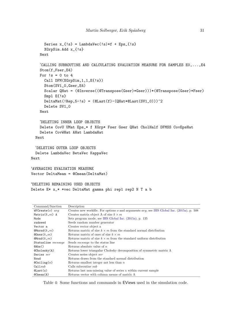
Martin Solberger, Erik Spanberg 31
Series x_!s = LambdaVec(!s)*f + Eps_!s
XGrpSim.Add x_!s
Next
'CALLING SUBROUTINE AND CALCULATING EVALUATION MEASURE FOR SAMPLES E0,...,E4
Stom(f,Fser,E4)
For !s = 0 to 4
Call DFM(XGrpSim,1,1,E!s)
Stom(SV1_0,Gser,E4)
Scalar QHat = (@Inverse((@Transpose(Gser)*Gser)))*(@Transpose(Gser)*Fser)
Smpl E!s
DeltaMat(!Rep,5-!s) = (@Last(f)-(QHat*@Last(SV1_0)))^2
Delete SV1_0
Next
'DELETING INNER LOOP OBJECTS
Delete CovU UMat Eps_* f XGrp* Fser Gser QHat CholHalf DFMSS CovEpsHat
Delete CovWHat AHat LambdaHat
Next
'DELETING OUTER LOOP OBJECTS
Delete LambdaVec BetaVec KappaVec
Next
'AVERAGING EVALUATION MEASURE
Vector DeltaMean = @Cmean(DeltaMat)
'DELETING REMAINING USED OBJECTS
Delete E* x_* *vec DeltaMat gamma phi rep1 rep2 N T a b
Command/function Description
WFCreate(o) arg Creates new workfile. For options o and arguments arg, see IHS Global Inc. (2015a), p. 508Matrix(k,m) A Creates matrix object A of size k ×mMode Sets program mode, see IHS Global Inc. (2015a), p. 135rndseed Seeds random number generatorVector a Creates vector object a@Mnrnd(k,m) Returns matrix of size k ×m from the standard normal distribution@Ones(k,m) Returns matrix of ones of size k ×m@Mrnd(k,m) Returns matrix of size k ×m from the standard uniform distributionStatusline message Sends message to the status line@Abs() Returns absolute value of n@Cholesky(A) Returns lower triangular Cholesky decomposition of symmetric matrix ASeries ser Creates series object serNrnd Returns draws from the standard normal distribution@Ceiling(n) Returns smallest integer not less than nCallsub Calls subroutine sub@Last(x) Returns last non-missing value of series x within current sample@Cmean(A) Returns vector with column means of matrix A
Table 4: Some functions and commands in EViews used in the simulation code.

32 EViews: Estimating a Dynamic Factor Model
References
Ahn SC, Horenstein AR (2013). “Eigenvalue Ratio Test for the Number of Factors.” Econo-metrica, 81, 1203–1227.
Anderson TW (2003). An Introduction to Multivariate Statistical Analysis. Wiley, New York.
Bai J (2003). “Inferential Theory for Factor Models of Large Dimensions.” Econometrica, 71,135–171.
Bai J, Li K (2012). “Statistical Analysis of Factor Models of High Dimension.” The Annalsof Statistics, 40, 436–465.
Bai J, Li K (2016). “Maximum Likelihood Estimation and Inference for Approximate FactorModels of High Dimension.” The Review of Economics and Statistics, 98, 298–309.
Bai J, Ng S (2002). “Determining the Number of Factors in Approximate Factor Models.”Econometrica, 70, 191–221.
Bai J, Ng S (2006). “Confidence Intervals for Diffusion Index Forecasts and Inference forFactor-Augmented Regressions.” Econometrica, 74, 1133–1150.
Bai J, Ng S (2007). “Determining the Number of Primitive Shocks in Factor Models.” Journalof Business & Economic Statistics, 25, 52–60.
Bai J, Ng S (2008). “Large Dimensional Factor Analysis.” Foundations and Trends in Econo-metrics, 3, 89–163.
Bai J, Ng S (2013). “Principal Components Estimation and Identification of Static Factors.”Journal of Econometrics, 176, 18–29.
Bai J, Wang P (2014). “Identification Theory for High Dimensional Static and DynamicFactor Models.” Journal of Econometrics, 178, 794–804.
Banbura M, Giannone D, Modugno M, Reichlin L (2012). “Now-Casting and the Real-TimeData Flow.” In G Elliott, A Timmermann (eds.), Handbook of Economic Forecasting,volume 2A. Elsevier-North Holland, Amsterdam.
Banbura M, Giannone D, Reichlin L (2011). “Nowcasting.” In M Clements, D Hendry (eds.),The Oxford Handbook of Economic Forecasting. Oxford University Press, Oxford.
Banbura M, Runstler G (2011). “A Look Into the Factor Model Black Box: PublicationLags and the Role of Hard and Soft Data in Forecasting GDP.” International Journal ofForecasting, 27, 333–346.
Bernanke BS, Boivin J, Eliasz P (2005). “Measuring the Effects of Monetary Policy: AFactor-Augmented Vector Autoregressive (FAVAR) Approach.” The Quarterly Journal ofEconomics, 120, 387–422.
Boivin J, Giannoni MP, Mihov I (2009). “Sticky Prices and Monery Policy: Evidence fromDisaggregaed US Data.” American Economic Review, 99, 350–384.

Martin Solberger, Erik Spanberg 33
Breitung J, Eickmeier S (2006). “Dynamic Factor Models.” Allgemeines Statistisches Archiv,90, 27–42.
Chamberlain G, Rothschild M (1983). “Arbitrage, Factor Structure, and Mean-variance Anal-ysis on Large Asset Markets.” Econometrica, 51, 1281–1304.
Diebold FX, Li C (2006). “Forecasting the Term Structure of Government Bond Yields.”Journal of Econometrics, 130, 337–364.
Diebold FX, Rudebusch GD, Aruoba SB (2006). “The Macroeconomy and the Yield Curve:A Dynamic Latent Factor Approach.” Journal of Econometrics, 131, 309–338.
Doz C, Giannone D, Reichlin L (2011). “A Two-Step Estimator for Large ApproximateDynamic Factor Models Based on Kalman Filtering.” Journal of Econometrics, 164, 180–205.
Doz C, Giannone D, Reichlin L (2012). “A Quasi-Maximum Likelihood Approach for Large,Approximate Dynamic Factor Models.” The Review of Economics and Statistics, 94, 1014–1024.
Durbin J, Koopman SJ (2012). Time Series analysis by State Space Methods. Oxford Uni-versity Pres, Oxford.
Eickmeier S (2007). “Business Cycle Transmission from the US to Germany - A StructuralFactor Approach.” European Economic Review, 51, 521–551.
Forni M, Giannone D, Lippi M, Reichlin L (2009). “Opening the Black Box: Structural FactorModels With Large Cross Sections.” Econometric Theory, 25, 1319–1347.
Forni M, Hallin M, Lippi M, Reichlin L (2000). “The Generalized Dynamic-Factor Model:Identification and Estimation.” The Review of Economics and Statistics, 82, 540–554.
Forni M, Hallin M, Lippi M, Reichlin L (2004). “The Generalized Dynamic Factor ModelConsistency and Rates.” Journal of Econometrics, 119, 231–255.
Forni M, Reichlin L (1998). “Let’s Get Real: A Factor Analytical Approach to DisaggretgatedBusiness Cycle Dynamics.” Review of Economic Studies, 65, 453–473.
Giannone D, Reichlin L, Small D (2008). “Nowcasting: The Real-Time Informational Contentof Macroeconomic Data.” Journal of Monetary Economics, 55, 665–676.
Hamilton JD (1994). Time Series Analysis. Princeton University Press, New Jersey.
Harvey AC (1989). Forecasting, Structural Time Series Models and the Kalman Filter. Cam-bridge University Press, Cambridge.
IHS Global Inc (2015a). “EViews 9 Command and Programming Reference.” Irvine CA, USA.
IHS Global Inc (2015b). “EViews 9 Object Reference.” Irvine CA, USA.
IHS Global Inc (2015c). “EViews 9 User’s Guide I.” Irvine CA, USA.
IHS Global Inc (2015d). “EViews 9 User’s Guide II.” Irvine CA, USA.

34 EViews: Estimating a Dynamic Factor Model
Koopman SJ, Shephard N, Doornik JA (1999). “Statistical Algorithms for Models in StateSpace Using SsfPack 2.2.” The Econometrics Journal, 2, 107–160.
Lutkepohl H, Kratzig M (2004). Applied Time Series Econometrics. Cambridge UniversityPress, Cambridge.
Ludvigson SC, Ng S (2007). “The Empirical Risk-Return Relation: A Factor Analysis Ap-proach.” Journal of Financial Economics, 83, 171–222.
Lutkepohl H (2007). New Introduction to Multiple Time Series Analysis. Springer, Berlin.
Onatski A (2010). “Determining the Number of Factors from Empirical Distribution of eigen-values.” The Review of Economic and Statistics, 92, 1004–1016.
Phillips PCB, Moon HR (1999). “Linear Regression Limit Theory for Nonstationary PanelData.” Econometrica, 67, 1057–1111.
Ritschl A, Sarferaz S, Uebele M (2016). “The U.S. Business Cycle, 1867-2006: A DynamicFactor Approach.” The Review of Economics and Statistics, 98, 159–172.
Schumacher C, Breitung J (2008). “Real-Time Forecasting of German GDP Based on a LargeFactor Model With Monthly and Quarterly Data.” International Journal of Forecasting,24, 386–398.
Stock JH, Watson MW (2002a). “Forecasting Using Principal Components from a LargeNumber of Predictors.” Journal of the American Statistical Association, 97, 1167–1179.
Stock JH, Watson MW (2002b). “Macroeconomic Forecasting Using Diffusion Indexes.” Jour-nal of Business and Economic Statistics, 20, 147–162.
Stoica P, Jansson M (2009). “On Maximum Likelihood Estimation in Factor Analysis - anAlgebraic Derivation.” Signal Processing, 89, 1260–1262.
van den Bossche FAM (2011). “Fitting State Space Models with EViews.” Journal of StatisticalSoftware, 41, 1–16.
White H (1982). “Maximum Likelihood Estimation of Misspecified Models.” Econometrica,50, 1–25.
Zhou X, Solberger M (2017). “A Lagrange Multiplier-Type Test for Idiosyncratic Unit Rootsin the Exact Factor Model.” Journal of Time Series Analysis, 38, 22–50.
Affiliation:
Martin SolbergerDepartment of StatisticsUppsala UniversityPO Box 513, SE-75120, Uppsala, SwedenE-mail: [email protected]: http://www.statistics.uu.se/