estimate optimization parameters for incoherent backscatter heterodyne lidar

Estimate optimization parametersfor incoherent backscatter heterodyne lidar

Barry J. Rye and R. Michael Hardesty

Heterodyne lidar estimates are a function of a number of experimental parameters, some of which can beadjusted or tuned to optimize statistical precision. Here we refer the precision to the theoretical limitfor optical measurements of return power and Doppler shift and investigate the conditions for optimi-zation using established theoretical expressions for the standard deviation of various estimates. Tuningis characterized by a degeneracy parameter ~the photocount per fade!. For estimators that filter orresolve the return, it is shown that optimal tuning is achieved at wideband signal-to-noise ratios less than0 dB and detected signal levels corresponding to more than a single effective photocount. Estimatorsthat do not filter are predictably at a disadvantage when the signal bandwidth range gate product is low.The minimum standard deviation available from an optimally tuned heterodyne system is found to begreater than twice the limit. © 1997 Optical Society of America

1. Introduction

The tuning of a heterodyne lidar used with incoherentbackscatter targets is central to its performance. It isknown in antenna theory, for example, that the max-imum signal-to-noise ratio available is limited by thestrength of the signal within a single coherence area,the photocount per spatial speckle.1 To maximize theheterodyne signal at a given level of shot noise, it fol-lows that the optics must be diffraction limited and thetransmitter and receiver optics focused to maximize anefficiency parameter.2,3 We are concerned here witha second example related to data processing. Bothsignal fluctuations and shot noise contribute sepa-rately to the precision of an estimate, which results ina requirement that the signal photocount per temporalspeckle period should be optimized. In this paper wefollow the practice in radar of refering to temporalspeckle as fading. This need to match the photocountand the fade count was realized in early research onreturn power estimation4–7 ~see Subsection 2.A!. A

B. J. Rye is with the Cooperative Institute for Research in Envi-ronmental Sciences ~University of Colorado and National Oceanicand Atmospheric Administration!, Environmental TechnologyLaboratory, 325 Broadway, Boulder, Colorado 80303. R. M.Hardesty is with National Oceanic and Atmospheric Administra-tion Environmental Technology Laboratory, 325 Broadway, Boul-der, Colorado 80303.

Received 11 April 1997; revised manuscript received 27 August1997.

0003-6935y97y369425-12$10.00y0© 1997 Optical Society of America

preliminary study ~see Fig. 7 of Ref. 8! showed that arather low signal-to-noise ratio is optimal for Dopplermeasurements, suggesting that these should also bedesigned with the low pulse energy needed to matchthe photocount and fade count.

Standard algorithms find both return power andDoppler shift by picking the peak in an optimallysmoothed spectrum of the data. The spectrum isobtained by Fourier transformation of a weighted es-timate of the autocorrelation function ~ACF! of thereturn that is calculated over several lags. The mea-surement equation for such peak-picker algorithms isnonlinear. A consequence is that estimates canjump discontinuously over values within the entirereceiver bandwidth in response to small changes insignal or noise values at low signal levels. Esti-mates in this limit are biased and have a non-Gaussian distribution ~e.g., Refs. 8 and 9!. To avoidthis, rectified data products ~the unweighted ACF orspectral estimates! are averaged prior to processing~data accumulation!.8 To acquire sufficient datausually entails use of a lidar operating at a high-pulserepetition frequency.10

High data throughput is therefore a common re-quirement of heterodyne lidars. The computationalcomplexity of these processing algorithms compoundsthe problem and leads to consideration of simplerestimators at least for real-time display purposes.In the simplest techniques, estimates of the meanparameters of the combined signal and noise can bedetermined by use of only an unweighted estimate ofthe ACF at a single lag and without explicitly forming

20 December 1997 y Vol. 36, No. 36 y APPLIED OPTICS 9425

a spectrum. For estimating mean power ~which isjust the zeroth lag!, one can square and average thetime-series signal. To estimate the mean frequency,the phase angle of the first lag of the ~complex! signalautocovariance can be used in what has come to becalled, from the way it is implemented in radar, thepulse pair algorithm.11

In this paper we examine the tuning requirementsfor some simple and sophisticated estimators ofpower ~Section 3! and Doppler shift ~Section 5! andcompare their performance under optimal tuningwith the theoretical limits for optical systems. It isimplicitly assumed that small signal bias is avoidedby use of adequate data accumulation that ~as weshow below! can be accomplished without affectingthe tuning conditions. The properties of the estima-tors considered here have generally been discussedpreviously and are only summarized in Sections 2and 4. This paper is based on papers given at co-herent lidar conferences in Keystone, Colorado~1995!, and Linkoping, Sweden ~1997!.

2. Power Estimators

A. Squarer

The simplest method for determining return power isto square the output of the photodetector ~which in aheterodyne receiver is used as a mixer so that its acoutput is proportional to the amplitude of the signal!and average the results. The squared data has amean value ^PS& 1 ^PN&. ^PS& here is the mean sig-nal. ^PN& is the mean measurement noise, which ina heterodyne system arises mainly from local oscilla-tor shot noise. It is assumed to be known, so thatthe estimation of ^PS& is equivalent to the estimationof the wideband signal-to-noise ratio ~SNR! d 5 ^PS&y^PN&. The statistics of the squared data are expo-nential so that the standard deviation ssqr~PS! 5 ^~PS1 PN!&. Thus the fractional standard deviation of anestimate based on a single data point is

ssqr~PS!

^PS&5

ssqr~d!

d5 1 1

1d

. (1)

On the right hand side of Eq. ~1! the second term 1ydarises from measurement noise and the first term fromfading in the signal itself. The asymptotic behavior ofthis result for low and high signals is characteristic ofall the estimators we consider in this paper and isworth discussing here because this estimator is thesimplest. It can be compared with what is expectedfor a direct detection system dominated by signal shotnoise, in which the fractional standard deviation of areturn power measurement is inversely proportionalto the square root of the signal strength or photocount@Eq. ~11! below#. From Eq. ~1!, at high signal levels ~d.. 1!, ssqr~PS! 5 ^PS& and ssqr~d!yd is independent ofsignal strength because the noise is dominated by~multiplicative! signal fading. This is the ultimatelimit for both heterodyne and direct detection lidarswith use of incoherent backscatter targets, although itis more commonly encountered with heterodyning be-

9426 APPLIED OPTICS y Vol. 36, No. 36 y 20 December 1997

cause the overall speckle count ~from both spatialspeckle and fading! is much lower. At low signal lev-els ~d ,, 1!, ssqr~dyd 5 1yd and diminishes inversely asthe signal strength, that is, more rapidly than for di-rect detection. Therefore this dependence cannotonly be the consequence of a high level of measurementnoise. It is attributable5 to small signal suppres-sion,12 that is, to the degradation of the small signalwideband SNR at the output of a nonlinear detector;heterodyne receivers need such detectors ~usually asquarer implemented in software! because their pho-todetector is used as a mixer and does not rectify theheterodyne output.

In early research,5–7 a short laser pulse was as-sumed to maximize fade averaging by ensuring thatsuccessive data values within a single range gatewere uncorrelated. For the data sample acquiredover a range gate containing M ~complex! data points,ssqr~d!yd 5 ~1y=M!~1 1 1yd!. For a heterodyne sys-tem, ^PN& can be written as ~QF!hnFS where FS is thereceiver ~or search! bandwidth and ~QF! is a noisefigure ~the ratio of actual noise power to the quantumlimit hnFS!. From Nyquist’s theorem, FS is also theminimum ~complex point! sampling frequency so thatFS 5 MyT where T is the time interval over whichdata within the range gate are collected. An effec-tive detected photocount Npc is defined by d 5 ^PS&y@~QF!hnFS# 5 NpcyM. Moreover, because the datapoints are independent, the fade count m 5 M. Itfollows that ssqr~d!yd 5 =m@~1ym! 1 ~1yNpc!#, fromwhich it was shown6,7 that optimal tuning, or mini-mal s~d! for a given signal level Npc, occurs at Npc 5m 5 M, that is, when the photocount and fade countare equal. At optimal tuning, ssqr~d!yd 5 2y=Npc.The results that follow, although they refer to differ-ent problems, all have similar characteristics.

If the lidar pulse is not short, the precision is notreduced by a factor =M because of the data pointcorrelation over the duration of a signal fade. Asshown in Appendix A @Eq. ~A3!#, it is reduced by afactor =meff where meff 5 MyW~Lumu2! is an effectivenumber of independent estimates of the return thatreflects the ~different! bandwidths of the signal andthe noise; W~Lumu2! is defined as the equivalentwidth13 of the function Lumu2 by W~Lumu2! 5 SkLkumuk

2;mk is the ACF of the photodetector output, and thetriangular function Lk 5 1 2 ukuy~M 2 1! ~uku , M! isthe ACF of the range gate weighting function. Fromthese definitions, W~Lumu2! has a minimum value of 1and meff a maximum value of M. The general ex-pression for the fractional standard deviation of asquarer becomes

ssqr~d!

d5

1

ÎmeffS1 1

1dD5 HFW~Lumu2!

NpcdGJ1y2 S1 1

1dD . (2)

B. Levin’s Maximum-Likelihood Spectral Estimator

An estimator of power that takes advantage of spec-tral filtering of the signal can be formed by one ap-plying a Fourier transform to the data and formingthe square modulus of the frequency components to

obtain the periodogram. The earliest algorithm forforming maximum-likelihood estimates of signal pa-rameters by smoothing the periodogram wasLevin’s,14 which is based on the assumption thatspectral components of the periodogram are uncorre-lated. Spectral correlation would arise from win-dowing of the time series and the consequenttruncation of the signal ACF, so that Levin’s is anapproximation in which the range gate is regarded asinfinite. A simple spectral domain-matched filter al-gorithm results. The associated formulas for theCramer–Rao lower bound ~CRLB! on estimate preci-sion illuminate the parameterization of the problemand ~as shown below! are an asymptotic limit onother estimates. We assume that the expectedvalue of the power spectral components is given by fi5 fi

~S! 1 fi~N! with white noise fi

~N! 5 1, and aGaussian signal spectrum

fi~S! 5 a1 expF2

~Fi 2 F1!2

2F22 G . (3)

If we further replace the summations over discretelysampled ~and range-gated! data values by integralsover continuous variables, the CRLB on the frac-tional standard deviation of the signal power esti-mate becomes15

sLevin~d!

d5

1

ÎNpc Îg0~a1!, (4)

where Fi is the frequency of the ith spectral compo-nent, F1 is the frequency shift to be determined, andF2 is the bandwidth of the signal. From Eq. ~3!, theparameter

a1 5d

Î2p f2

5Npc

Î2p f2M, (5)

is the peak SNR in the spectral density of the ungatedsignal and f2 5 F2yFs. In Eq. ~4!,

g0~a1! <a1

Î2p *2`

` exp~2x2!dx@1 1 a1 exp~2x2y2!#2 . (6)

As expected, the range gate does not appear explic-itly in the Levin equations. In Eq. ~4! the fractionalstandard deviation of the power measurement de-pends only on Npc and a1, so that for a given signalstrength, a1 is the tuning parameter. The reasonwhy a1 determines the balance between the photo-count and the fade count can be seen by a consider-ation of the final term in Eq. ~5! where the numeratoris the effective photocount and the denominator con-tains the time–bandwidth or signal bandwidth rangegate product F2T 5 f2M, which is a measure of thefade count within the range gate.

C. Brovko–Zrnic Time-Domain Maximum-LikelihoodAlgorithm

The optimal maximum-likelihood estimator for theparameters of stationary time series with Gaussian

statistics is attributed by Zrnic16 to Brovko and takesinto proper account the discreteness of the data andthe range gate window. Results differ from Levin’swhen the duration of the range gate window is lessthan the correlation time constant of the return sig-nal, that is ~roughly!, when f2M , 1. The algorithmcan also be regarded in terms of spectral domain-matched filtering, but the weighting is applied toterms in the estimated ACF in the time domain anddepends on the position of the contributing data sam-ple values within the range gate.16 The equationshave been discussed by a number of authors mainlyin the radar literature, but simple and computation-ally efficient expressions for the CRLB were not dis-covered until the recent work of Frehlich.17 To beconsistent with the assumption of a Gaussian signalspectrum @Eq. ~3!#, terms within the ACF of an un-gated signal time series are assumed to be

mk~S! 5 umk

~S!uexp~ j2pf1k!

5 exp@2~2pf2k!2y2#exp~ j2pf1k!, (7)

where f1 5 F1yFS. The kth term in the ACF of thedata ~the signal plus a white noise! is

mk 5mk

~S!d 1 mk~N!

1 1 d, where mk

~N!

5 1~k 5 0!, mk~N! 5 0 otherwise. (8)

The CRLB is expressed in terms of the elements gik ofthe signal covariance matrix G, where

gik 5 umuk2iu~S!u 5 exp@2~2pf2uk 2 iu#2!y2# (9)

together with the elements qik and gik of the matricesQ 5 Gd 1 I, and G 5 Q21, where I 5 diag~1, 1, . . . ,1! is the identity matrix @our definition of Q differsfrom Frehlich’s by a constant factor ~the noise level!,but this does not affect the result#. Using Frehlich’sEqs. ~3! and ~11!, we obtain, for the CRLB on thevariance of the wideband SNR d estimate,

sBZ2~d! 5

1

trSG ]Q]d

G]Q]dD

51

tr~AA!5

1

(i50

M21

(k50

M21

aikaki

. (10)

where A 5 GG and aik 5 Smgimgmk.

3. Parameters of Heterodyne Systems TunedOptimally for Return Power Measurement

A. Parameterization

The optimum fractional standard deviation of apower measurement in the absence of backgroundnoise is achieved in a photon-counting ~incoherent!system that yields a fractional standard deviation

sopt~d!

d5

1

ÎNpc

, (11)

where Npc is the actual photocount. Equations ~2!and ~4! were written so that the dependence on the


effective photocount for a heterodyne receiver ~alsoNpc! is apparent. Levin’s expression is especiallysimple in that the tuning is described by the singleparameter a1. These observations suggest that theperformance of a suboptimal estimator with a stan-dard deviation s~d! could be characterized by oneplotting

~EF!0 5 F s~d!

sopt~d!G2

5 NpcFs~d!

d G2

(12)

as a function of a1. ~EF!0 can be regarded as thenoise figure of the suboptimal power or the widebandSNR estimate because it quantifies the power withinthe noise fluctuations in the estimate compared withthe theoretical ideal.

In Fig. 1, we plot s~d!yd against the signal level Npcfrom Eqs. ~2!, ~4!, and ~10! for heterodyne estimatorswith particular parameters that are described in thecaptions. Each curve displays the dependence on1yNpc ~not Npc

21y2! for low signals and the indepen-dence of Npc for high signals that is similar to thatdiscussed in Subsection 2.A for the squarer. Theprecision of each estimate improves monotonicallywith increasing signal level. However, we can ob-tain the best performance at a given value of Npc byoperating where the heterodyne curves lie closest tothe 1y=Npc line; if necessary, accumulation could beused to increase the photocount and the fade countsimultaneously, thus keeping the tuning parametera1 constant.18 In Fig. 2 we plot noise figures ~EF!0as a function of a1; use of sLevin~d! is compared withuse of ssqr~d! in Fig. 2~a! and with use of theBrovko–Zrnic ~BZ! formula sBZ~d! in Fig. 2~b!. For

Fig. 1. Fractional standard deviation for a return power measure-ment plotted against the signal energy measured as an effectivephotocount Npc. The straight line is the theoretical limit for anyoptical system, s~d!yd 5 1y=Npc @Eq. ~11!#, and the solid curvegives Levin’s CRLB @Eqs. ~4–6!# for a heterodyne lidar with f2 50.141, M 5 10, i.e., a time–signal bandwidth F2T 5 f2M . 1. Inthis regime, it is expected that the Brovko–Zrnic CRLB @Eq. ~10!,shown here as open squares# would give similar results to Levin.The squarer @Eq. ~2!, crosses# leads to slightly inferior performanceat both low and high signal levels. All the curves for heterodyneestimates have the fractional standard deviation asymptoticallylinear in 1yNpc at low signal and independent of Npc at high signal.


each case, the minimum in the tuning curves movesaway from the Levin value and to higher a1 as M isreduced. Careful comparison of the curves for theBZ algorithm and for squaring shows that the filter-ing assumed in the BZ algorithm improves its esti-mate at low values of a1 when the widebandbackground noise ~local oscillator shot noise! domi-nates signal fading and filtering is advantageous.

The shapes of the log–log plots of the tuning curvesin Fig. 2 are obviously similar and can be comparedwhen each ordinate is divided by its value at its min-imum ~EF!0

~min! and each abscissa is divided bya1

~min!, so that the coordinates of all the minima are~1, 1!. An example is shown in Fig. 3. Curves forthe squarer are symmetrical and slightly narrowerthan those from sBZ~d!. In both cases, the valleysaround the minima are quite broad; an order-of-magnitude variation of the tuning parameter a1 fromthe minimum increases ~EF!0 by a factor of less than4; thus the quality of the tuning is not critical.

The similarity in the shapes of the curves encour-ages us to argue that the results can be largely char-acterized by just plotting the coordinates of theminima in the tuning curves. These minima aresignificant in their own right because they define theoptimal tuning of heterodyne systems. In Figs. 4and 5, ~EF!0

~min! and a1~min! are plotted as a function

of the time–bandwidth product for selected values ofM. The tuning parameter a1

~min! gives the value ofNpc at which performance is optimized for given f2and M, and the performance parameter ~EF!0

~min!

gives the smallest factor by which the variance ex-ceeds the theoretical limit. Because the curves inFigs. 4 and 5 are plotted for constant M, we refer tolow values of f2M as the low bandwidth or long-pulselimit and small values as the large bandwidth or, forbrevity, the short-pulse limit; the latter conceals thepossibility that a large lidar signal bandwidth couldalso result from modulation either in the transmitteror by the scattering particles.

B. Optimal Tuning

Figure 4 shows the tuning parameter for returnpower estimates obtained with use of ssqr~d! andsBZ~d!. Of all the figures here, it is perhaps the onemost amenable to physical interpretation. As it is alog–log plot, straight lines of slope 21 indicate con-stant values of Npc 5 =~2p!a1f2M. A curve for tun-ing of the squarer follows such a line with Npc 5 M,provided the pulse is sufficiently short that the time-series data are uncorrelated. Roughly, this requiresf2 . 0.28 ~see Appendix A, Eq. ~A8! for M 5 1!. Thisis in agreement with the conclusion reached for theshort-pulse limit in Subsection 2.A when the numberof fades is limited to its maximum value M.

Values of a1 for optimally tuned systems with useof the BZ CRLB are also shown in Fig. 4. There arethree distinct regimes. In the short-pulse limit, fil-tering does not change the estimate or the tuningparameter so that the results are the same as for thesquarer, and the curves follow the Npc 5 M line. Inthe long-pulse limit, when the number of indepen-

Fig. 2. ~a! The estimator noise figure, the ratio of the normalizedvariance of a return power measurement to its theoretical limit @Eq.~12!# is plotted as a function of the tuning parameter a1. The use ofsLevin @Eq. ~4!, solid curve with small open squares# that is indepen-dent of M is compared with values obtained from ssqr~d! @Eq. ~2!#.The squarer estimates were obtained with the relative signal band-width f2 5 0.0044. The curve for M 5 64 ~curve with downward-pointing triangles! corresponds to a time–bandwidth product f2M 51y~2=p! so that the range gate is matched to the bandwidth of thereturn @Appendix A, Eq. ~A8!#. At high a1 the performance of thissquarer is approximately described by Levin’s formula. Similarresults could be obtained for nonmatching gates with M . 64; as therange gate is reduced below the length of the pulse, Levin’s approx-imation is no longer valid. Curves are shown for M 5 10 ~thincurve! and M 5 2 ~curve with upward-pointing triangles!; the resultsfor M 5 10 are supported by values obtained from simulations ~largeopen squares!. At low a1 all the squarer curves coincide becausethe noise figure for squarer estimates is independent of M; this resultcan be derived easily from Eq. ~2!. ~b! As Fig. 2~a!, except thecomparison here is between values obtained from sLevin~d! @Eq. ~4!#and from sBZ~d! @Eq. ~10!#. A reduction in the range gate ~whichmakes the correlation time of the signal longer than the range gate!again shifts the BZ curves to higher a1, but here the noise figure atlow a1 depends on both f2 and M, and the minimum for all thesecases is approximately 4. In the simulations leading to the resultsfor M 5 10, f2 5 0.0044 ~large open squares!, the wideband SNR wasobtained by iteration of the BZ algorithm to maximize the log like-lihood ratio, as described in Ref. 21.

dent fades ~meff, not f2M! is unity, optimum tuning ofthe BZ algorithm is obtained along the line Npc 5 1.Between these two limits, within the intermediateregime with f2M of order 1, a1 varies only slightly andtends asymptotically toward the Levin value @a1

~min!

5 1.46, shown by the arrow# as the range gate be-comes longer relative to the bandwidth. The tran-sition to the short-pulse regime occurs when eachcurve crosses the Npc 5 M line, which is again ap-proximately when f2 5 0.28. The transition to thelong-pulse limit occurs approximately when therange gate is matched to the return signal in thesense that the equivalent widths, or integral scales, ofthe ACF’s of the gate window and the return signalare equal @see Appendix A, Eq. ~A8!#; for the Gaussiansignal ACF this occurs at f2M 5 1y~2=p! ' 0.28,which is also shown by an arrow.

Corresponding values of the =~EF!0~min! that we

obtained using ssqr~d! and sBZ~d! are shown in Fig. 5.The square root of the noise figure is used because itcorresponds to the fractional standard deviation ofthe estimate. The lowest noise figure, which is 4,from sBZ~d! is ~somewhat surprisingly! obtained inthe short-pulse and long-pulse regimes, whereas inthe intermediate regime ~EF!0

~min! is slightly in-creased. The increase is at most only approximately5%, which makes sBZ~d! in this regime about thesame as that predicted by Levin’s algorithm. The

Fig. 3. Comparison of return power estimator noise figure curves@as those shown in Figs. 2~a! and 2~b!# that are displaced so thattheir minima are superimposed. The Levin curve @Eq. ~4!# isagain shown as a solid curve marked by small open squares. BZcurves @Eq. ~10!# are shown for matched systems @ f2M 5 1y~2=p!,Eq. ~26!# with M 5 2 ~dashed curve!, M 5 10 ~large open squares!,and M 5 64 ~thin curve!. The thin curve marked by filleddownward-pointing triangles is calculated for the squarer with Eq.~2! by our assuming a matched system with M 5 64. The thincurve marked by upward-pointing triangles is obtained for M 5 1with use of either the squarer or the BZ formulas. The conclu-sions to be drawn are that, for the matched system ~or, in fact, forsystems with longer range gates than required for matching!, theshape of the Levin curve is a reasonable approximation for theshapes of curves obtained from the BZ CRLB, especially at low a1,and that the shape of curves for the squarer are symmetrical andsomewhat narrower than that obtained from Levin.


squarer achieves the BZ bound in the short-pulselimit, but when the intermediate regime is entered itsnoise figure increases sharply, especially for large M.As we commented in Subsection 3.A, this occurs be-cause spectral filtering is beneficial when the returnbandwidth is narrow relative to the range gate. Inthe long-pulse limit, the noise figure of the squarerlevels off.

It is noteworthy that, in the long-pulse and inter-mediate regimes for the range of M shown, the BZcurves overlap in both a1

~min! and EF0~min! plots and

are therefore functions of only the time–bandwidthproduct f2M; hence, sBZ

2~d! } Npc~EF!0~min! is a func-

tion of only Npc and f2M. This observation is inagreement with that of Frehlich and Yadlowsky9 forthe dependence of the BZ CRLB for estimates of theDoppler shift. However, the transition to the short-pulse regime is determined only by M and is essen-tially independent of f2 ~Fig. 4!.

4. Doppler Estimators

In this section we summarize the formulas forCRLB’s on the Doppler estimator given by the Levinand the BZ filters with the standard deviation of thepulse pair or first lag covariance estimator, which isa single lag estimator of the mean frequency of thedata that occupies a somewhat similar position withregard to Doppler estimation as the squarer estima-tor for return power.

In the pulse pair algorithm the mean frequency of

Fig. 4. Tuning parameter a1~min! of optimally tuned heterodyne

lidars used for return power measurements with squaring and theBZ algorithm are plotted against the time–signal bandwidth prod-uct f2M. Values for optimally tuned systems with use of sBZ~d!are shown for M 5 2, 10, and 64 with increasingly heavier solidcurves. These curves overlap exactly at low f2M. Values for op-timally tuned squarers are shown for M 5 1 ~open squares withcrosses!, M 5 2 ~crosses!, and M 5 64 ~open squares!. Thestraight diagonal dotted lines correspond to constant Npc 5 a1=~2p!f2M 5 1, 2, 10, and 64 and indicate asymptotic limits for thecurves at high f2M. The tuning parameter obtained from theLevin formula a1

~min! 5 1.46 is indicated by a horizontal arrow, andthe vertical arrow indicates the value of f2M 5 1y~2=p! obtainedfor a system in which the range gate and signal bandwidth arematched in the sense of Eq. ~26!.


the data is inferred from the phase angle of the firstlag complex covariance.11 If the data are collectedover a range gate containing M . 2 ~complex! points,then there are M 2 1 estimates of the first lag co-variance available from contiguous data points thatare correlated. These estimates are not indepen-dent, and the variance of the sample is not simply1y~M 2 1! times the variance of each estimate. Aformula is given by Zrnic,19 which becomes, in thecurrent notation,

spp2~ f1! 5

18p2~M 2 1!um1

~S!u2

3 H1d2 1

2d F1 2

M 2 2M 2 1

um2~S!uG

1 W@um~S!u2L#@1 2 um1~S!u2#J, (13)

where m~S! was defined in Eq. ~7! and W@m~S!L# wasdefined in the discussion of Eq. ~2!.

The CRLB for frequency shift estimates obtainedwith Levin’s approximation is14

sLevin~ f1! 5f2

ÎNpc Îg1~a1!, (14)

Fig. 5. Square root of the estimate noise figure of optimally tunedheterodyne lidars used for return power measurements withsquaring and the BZ algorithm. The square root is shown be-cause it corresponds directly to the fractional standard deviation ofthe estimate. The symbols and curved lines correspond to those ofFig. 4, except that open circles indicate results for the squarer withM 5 10, and results for the squarer with M 5 1 are not shown ~theyhave the constant value 2.0!. The lowest noise figure with use ofsBZ~d! is obtained in the short-pulse and long-pulse regimes. Inthe intermediate regime ~Fig. 4! the standard deviation is de-graded by a small factor of less than 5%, which makes sBZ~d! in thisregime about the same as sLevin~d!. Levin’s value from the opti-mal noise figure ~EF!0

~min! ;4.17 is marked by the horizontal ar-row. In the short-pulse limit, the squarer achieves the BZ limit,but when the transition regime is entered its noise figure increasessharply, especially for large M. In the long-pulse limit, the noisefigure of the squarer levels off @for M 5 64, this occurs at ~EF!0

~min!

' 17.6# ~not shown!.

where

g1~a1! 5a1

Î2p *2`

` x2 exp~2x2!dx~1 1 a1 exp~2x2y2!2!

. (15)

Equations ~14! and ~15! have obvious similaritieswith Eqs. ~4! and ~5!.

The CRLB obtained with the BZ algorithm can beobtained directly from Frehlich’s Eq. ~15!17:

sBZ2~ f1! 5

1

24p2 (i50

i5M21

(k50

k5M21

ui 2 ku2 qik gki

, (16)

where q and g are elements of the matrices Q and Gdefined in Subsection 2.C.

5. Parameters of Heterodyne Systems TunedOptimally for Doppler Measurement

The expression for the optimal standard deviation ofa Doppler-shift estimate with use of a photon-counting system, in conjunction with a bank of loss-less optical filters with no cross talk and for theGaussian signal spectrum of Eq. ~3!, is8

sopt~ f1! 5f2

ÎNpc

. (17)

By analogy with Eq. ~12! of Section 3, we can define anoise figure for any other estimator with a standarddeviation s~ f1! as

~EF!1 5 F s~ f1!

sopt~ f1!G2

5 NpcFs~ f1!

f2G2

. (18)

The performance of heterodyne systems used forDoppler estimation can be characterized by curvesqualitatively similar to those of Figs. 1–2 for returnpower estimation. A graph that is analogous to thatin Fig. 3, showing the shape of superimposed tuningcurves for matched systems at M 5 2, 10, and 64, isgiven in Fig. 6~a!. The conclusions to be drawn aremuch the same as for the return power estimators,except that the differences between results obtainedwith spp~ f1! and sBZ~ f1! at a1 .. a1

~min! are morepronounced. We also show a similar set of curves inFig. 6~b! for the case M 5 10, with f2 5 0.2y~2=p!,1y~2=p!, and 5y~2=p!, that is, with pulses that areboth longer and shorter than necessary for matchingto the range gate @see Eq. ~A8! in Appendix A#. Thepulse pair curves are symmetrical about their min-ima and, as before, are clustered together separatelyfrom the cluster of BZ curves. Comparison of Figs.6~a! and 6~b! supports the conclusion of Subsection3.A that performance can be largely characterized fora given estimator by the coordinates of the tuningcurve minima, which is obviously valid to a good ap-proximation in the important region around the min-imum.

The coordinates of the minima for Doppler estima-tion are given in Figs. 7 and 8, which can be usefullycompared with Figs. 4 and 5 for the return power

Fig. 6. ~a! Comparison of Doppler-shift estimator noise figurecurves that have been displaced so that their minima are super-imposed ~compare with Fig. 3!. The Levin curve @Eqs. ~14! and~15!# is again shown as a heavy curve marked by small opensquares, and the other curves are plotted for systems withmatched signal bandwidth and range gate @see Eq. ~A8! in Ap-pendix A#. Curves are plotted with sBZ

2 ~ f1! @Eq. ~16!# ~M 5 64is shown by the thin curve largely hidden below Levin line; M 510 is shown by the open squares!, and spp

2 ~ f1! @Eq. ~13!# ~M 5 64is shown by the thin curve with downward-pointing triangles;M 5 10 is shown by the open circles!. The curve for M 5 2~dashed curve! is the same for both algorithms. ~b! Comparisonof displaced Doppler-shift estimator noise figure curves as in Fig.6~a! for a fixed range gate M 5 10 and with varying relativesignal bandwidth f2. Curves with matched signal bandwidthand range gate @ f2M 5 1y~2=p!, Eq. ~A8! in Appendix A# areshown as a heavy curve with open small squares @BZ CRLB, Eq.~16!# and a light curve with filled squares @pulse pair, Eq. ~13!#,respectively. Curves with f2M 5 0.2y~2=p! ~in the long-pulseregime! are shown as large open squares ~BZ! and open circles~pulse pair!; curves with f2M 5 5y~2=p! are shown as a thincurve ~BZ, largely hidden! and a dashed curve ~pulse pair!. Theconclusions to be drawn are similar to those in Fig. 3, except thatthe Levin curve is not quite as good a fit to the BZ results iff2M ,, 1y~2=p!.


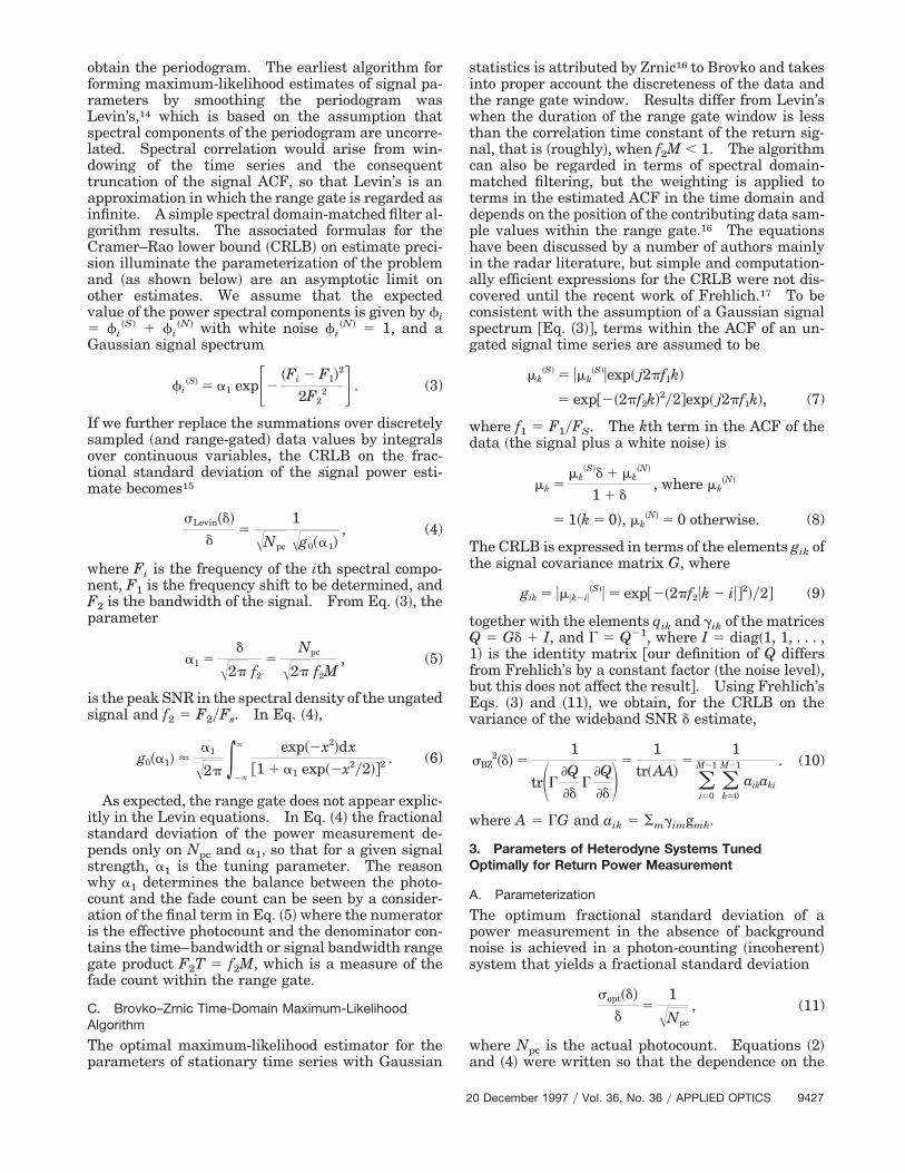
estimators. Figure 7 has obvious similarities withFig. 4. In the long-pulse limit, where the signal canbe regarded approximately as monochromatic, the BZperformance for all f2 and M is optimized at the samea1 as the pulse pair estimator at M 5 2. In theintermediate regime, a1

~min! remains a function onlyof f2M and decreases toward the Levin value as thepulse is shortened until Npc ; M; here, in contrast toFig. 4, there is a slight overshoot, but as f2M in-creases in the short-pulse regime, the curve for theBZ bound approaches those for the pulse pair and theline Npc 5 M. In this limit, the pulse pair algorithmleads to the BZ bound for a given M because the firstlag of the autocovariance carries all the informationand further filtering is not advantageous. Becausethe Levin value for a1

~min! is rather greater than inFig. 4, the geometry of the diagram ensures thattransition to the short-pulse regime occurs at a lowervalue of f2M.

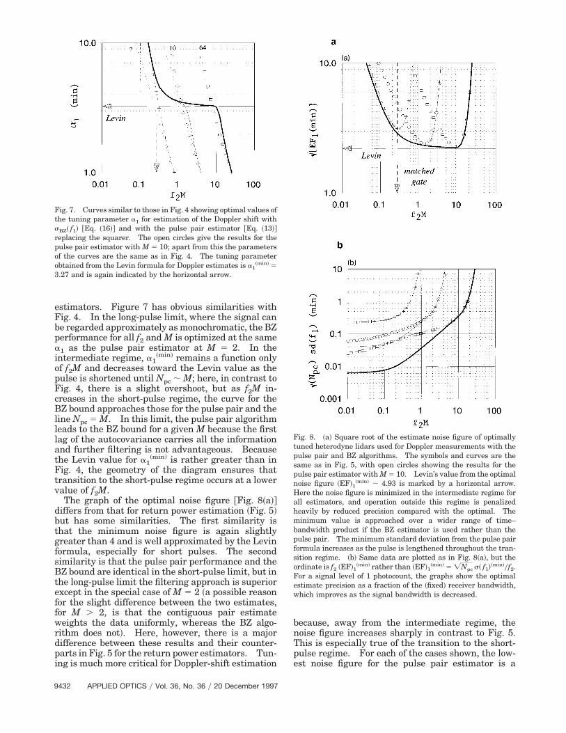
The graph of the optimal noise figure @Fig. 8~a!#differs from that for return power estimation ~Fig. 5!but has some similarities. The first similarity isthat the minimum noise figure is again slightlygreater than 4 and is well approximated by the Levinformula, especially for short pulses. The secondsimilarity is that the pulse pair performance and theBZ bound are identical in the short-pulse limit, but inthe long-pulse limit the filtering approach is superiorexcept in the special case of M 5 2 ~a possible reasonfor the slight difference between the two estimates,for M . 2, is that the contiguous pair estimateweights the data uniformly, whereas the BZ algo-rithm does not!. Here, however, there is a majordifference between these results and their counter-parts in Fig. 5 for the return power estimators. Tun-ing is much more critical for Doppler-shift estimation

Fig. 7. Curves similar to those in Fig. 4 showing optimal values ofthe tuning parameter a1 for estimation of the Doppler shift withsBZ~ f1! @Eq. ~16!# and with the pulse pair estimator @Eq. ~13!#replacing the squarer. The open circles give the results for thepulse pair estimator with M 5 10; apart from this the parametersof the curves are the same as in Fig. 4. The tuning parameterobtained from the Levin formula for Doppler estimates is a1

~min! 53.27 and is again indicated by the horizontal arrow.


because, away from the intermediate regime, thenoise figure increases sharply in contrast to Fig. 5.This is especially true of the transition to the short-pulse regime. For each of the cases shown, the low-est noise figure for the pulse pair estimator is a

Fig. 8. ~a! Square root of the estimate noise figure of optimallytuned heterodyne lidars used for Doppler measurements with thepulse pair and BZ algorithms. The symbols and curves are thesame as in Fig. 5, with open circles showing the results for thepulse pair estimator with M 5 10. Levin’s value from the optimalnoise figure ~EF!1

~min! ; 4.93 is marked by a horizontal arrow.Here the noise figure is minimized in the intermediate regime forall estimators, and operation outside this regime is penalizedheavily by reduced precision compared with the optimal. Theminimum value is approached over a wider range of time–bandwidth product if the BZ estimator is used rather than thepulse pair. The minimum standard deviation from the pulse pairformula increases as the pulse is lengthened throughout the tran-sition regime. ~b! Same data are plotted as in Fig. 8~a!, but theordinate is f2 ~EF!1

~min! rather than ~EF!1~min! 5 =Npc s~ f1!~min!yf2.

For a signal level of 1 photocount, the graphs show the optimalestimate precision as a fraction of the ~fixed! receiver bandwidth,which improves as the signal bandwidth is decreased.

function of f2 rather than f2M and is obtained whenthe equivalent width of the signal approximatelymatches that of a range gate with M 5 2, or when f2' 0.14 @Eq. ~A8! in Appendix A#. This agrees wellenough with the early result of Miller and Roch-warger,11 f2 ' 1y~2.4p! 5 0.13, that was obtained forthe precision obtained with noncontiguous pairswithout reference to the optimum available to opticalsystems @Eq. ~17!#. The short-pulse behavior of thepulse pair and BZ algorithms is identical, so that thecondition f2 ' 0.14 also determines when the BZcurves enter the transition to the short-pulse regime.

A further similarity with Fig. 5 is that the noisefigures obtained with sBZ~ f1! are the same at all M inthe long-pulse limit. This result follows from ourparameterization and, although valid, could be mis-leading. The noise figure of Eq. ~18! contains f2 inthe numerator. To obtain the absolute value ofsBZ~ f1! 5 ~ f2y=Npc!=~EF!1 at optimal tuning and fora given signal level, the values in Fig. 8~a! should bemultiplied by f2. It follows that the absolute preci-sion of the Doppler estimate improves monotonicallyas the bandwidth of the return diminishes, althoughthe improvement becomes increasingly incrementalif the pulse length becomes much longer than therange gate. This is shown in Fig. 8~b!.

6. Conclusions

We have referenced the statistical precision availablefrom unbiased heterodyne lidar estimators of returnpower and Doppler shift using incoherent backscatterwith extended ~deep! targets to that theoreticallyavailable from photon-limited lidars. These sys-tems are parameterized by the total signal energy~characterized by Npc! and peak SNR in the spectraldensity a1 that also measures the photocount perfade of the signal ~Subsection 2.B!. Although in-creasing Npc always improves the standard deviationin absolute terms, the performance relative to theideal is characterized by a1. Physically, this arisesbecause a1 determines the major source of noise; fora1 . 1, the noise arises from fading and for a1 , 1from wideband sources within the receiver. If a1 .1, an increase of the signal energy improves the ab-solute precision toward an asymptotic limit but de-creases the estimate precision relative to the ideal; ifa1 , 1, a decrease of signal energy not only reducesthe absolute precision as would be expected, but itagain decreases the relative precision ~the reason forthis, at least in the case of the squarer estimator forreturn power, is identified in Subsection 2.A withsmall-signal suppression!.

Both of these limits are relevant to the comparisonof heterodyne and direct detection systems. In stud-ies of statistical optics, the photocount per coherencecell ~which is equivalent to the photocount per spatialspeckle per fade and is measured by a1! is referred toas the photocount degeneracy parameter and is re-lated to the photon occupation number for thesource.20 Light from thermal sources ~including theSun! is nondegenerate ~a1 , 1!, as a result of whichheterodyne systems are insensitive to thermal

sources and background. This is one of the majoradvantages of using heterodyning for atmosphericmeasurements, especially in the daytime. Incoher-ently backscattered light is quasi-thermal orpseudothermal—that is, it shares the statistics ofthermal light, but in this case the degeneracy may beeither greater or less than 1 depending on thestrength of the backscatter. With such a source, theinsensitivity of heterodyne systems to return signalswith low degeneracy is a disadvantage. The prob-lems of designing heterodyne systems to average fad-ing, as needed for return signals with highdegeneracy, are well known if sometimes exagger-ated.

The plots of the tuning and performance parame-ters @a1, ~EF!0 and ~EF!1# at optimal tuning have beenshown to offer a useful and compact summary of thecapabilities of heterodyne systems and are the prin-cipal result of this discussion. For both power andDoppler shift, the standard deviation of estimatesobtained from optimally tuned systems with Gauss-ian signal spectra is rather more than twice the the-oretical limit ~Figs. 5 and 8!. Optimal tuningrequires that 1 # Npc # M, or 1yM # d # 1, forreturn power estimation ~Fig. 4! and ~approximate-ly! 3 # Npc # M, or 3yM # d # 1, for Dopplerestimation ~Fig. 7!. These limits are summarizedroughly by Npc . 1, d , 1.

These signal levels are low and can be below thethreshold needed to generate unbiased estimateswith a high confidence level. We have shown previ-ously that a1 can be used to parameterize this thresh-old.21 The threshold is at Npc ' 50 if a1 . 1, but itincreases for lower a1. If optimal tuning is achievedonly if Npc # M, accumulation of data products fromsystems that exploit spatial and temporal specklediversity is often a necessary rather than just a de-sirable goal. In discussions of accumulation, a1 hasthe useful property of being independent of accumu-lation order because the photocount and fade countincrease in step. In a practical system, signal levelsvary with range, and it is likely that optimal tuningcan be achieved at no more than one range. It ishere that the breadth of the tuning curves is gratify-ing, because they indicate noise figures less than tentimes the minimum over a band greater than 0.1 , a1, 100 ~Figs. 3 and 6!.

If the conditions for optimal tuning are much thesame for measurements of both power and Dopplershift, why are the former regarded as more difficult?The reason follows from Eqs. ~11! and ~17! ratherthan from the tuning criteria. In Eq. ~17!, f2 typi-cally corresponds to speeds of approximately 1 mys,so that to achieve a measurement with a precision of,say, 20 cmys calls for few more photocounts than areneeded to assure a high confidence level ~Npc ; 100!.From Eq. ~11!, this signal level would lead only to afractional standard deviation of the power estimate of~at best! 20% which is unlikely to be adequate.

The tuning parameters for computationally less in-tensive single lag estimators ~squarers and pulsepair! have been included in this study. Apart from


the practical utility of these algorithms, their prop-erties set asymptotic limits for the more sophisticatedestimators. They offer similar optimal performancein restricted regimes, approximately when f2 . 0.28for power estimates and when f2 ; 0.14 for Doppler,that is, when the filtering capability of a multilagalgorithm is not needed ~Figs. 5 and 8!. Away fromthe minima, their tuning curves are narrower ~Figs. 3and 6!. The principal advantage of the more com-plex algorithms can therefore be summarized by thestatement that they have broader tuning character-istics.

Appendix A: Variance and Equivalent-WidthCalculations for the Squarer

Our purpose in this appendix is to derive the stan-dard formula for the effective number of independentdata values for the squarer power estimator used inEq. ~2! and to justify the definition of the matchedrange gate used in some of the examples displayed inthe figures.

The action of the squarer is to replace the in-phase and quadrature components of the discretecomplex data time-series zi generated in the het-erodyne receiver with the series yi of square mod-ulus values:

yi 5 uzi u2. (A1)

The variance var~y! and the ACF m~y! are derived inthe usual way from the zero mean time-series Dyi 5yi 2 ^y&, where ^y& is the mean of y as var~y! 5^~Dyi!

2& and ~for the kth term of the ACF! mk~y! 5

^~Dyi!~Dyi1k!&yvar~y!; here ACF’s are normalized sothat the zero lag term is unity. If the ACF of theoriginal times-series z is written as m, then the ACFof the squared series y is m~y! 5 umu2. If only Mvalues of yi ~0 # i , M! are available over a rangegate, then the kth term of the ACF is defined by

umuk2 5 E1 1M 2 k

(i50

~M2k!21

DyiDyi1k

var~y!2 , (A2)

where E is the expected value.The average power within the range gate is the

average of the y values or ^P& 5 E@~1yM!Siyi# 5 ^y&.When we write DPi 5 Pi 2 ^P& 5 SjDyi, the varianceis

var~P! 51

M2 ^DP!2&,

..

51

M2 K(i50

M21

~Dyi! (j50

M21

~Dyj!L,

..

51M (

k52~M21!

M21 FS1 2uku

M 2 1Dumuk2Gvar~y!. (A3)


This can be written as var~P! 5 var~y!ymeff wheremeff is the effective number of independent data val-ues contributing to the estimate of P. meff is there-fore defined by

meff 5M

W~Lumu2!,

..

W~L umu2! 5 (k52~M21!

M21

Lk umuk2,

..

Lk 5 1 2 ukuy~M 2 1!. (A4)

Functions written here as W@ f ~x!#, and defined as inEq. ~A3!, are the equivalent widths13 of the discretefunctions f ~x!, measured as a ~noninteger! numberof increments; for this to be meaningful, the dis-crete function must be normalized with f ~x0! 5 1.0.The equivalent width is a measure of the coherencelength ~in increments! of a discrete random func-tion13 that is analogous to the integral scale of acontinuous ACF. L is the normalized ACF of thetop-hat windowing function, Pi 5 1y~M 2 1! ~0 # i ,M!; Pi 5 0 otherwise, that is used to isolate therange gate. The ACF of the squared waveform af-ter windowing is then Lumu2. Equations ~A3! and~A4! exemplify a standard result for the square of aquantity that is formed by one adding or averaginga random variable over a discrete zone, which hasbeen obtained both in the temporal ~as here! andspatial ~antenna! domains in different contexts andfor continuous and discrete variables ~e.g., Ref. 2!.From the definition of m used here and given in Eq.~8!, it can be seen that m is a weighted mean of theACF’s of the signal and the noise. Its equivalentwidth takes into account the different time scales ofthese two components so that each is averaged cor-rectly.

To obtain the ACF of estimates of P and its equiv-alent width, it is useful to regard sample values of Pas the output of a convolution operation on y by afilter with impulse response P. Then

DPj 5 (i50

M21

Pi~Dy!j2i or DP 5 PpDy. (A5)

Because P is a real, even function, this can also bewritten as the cross correlation of P and Dy, or DP 5P , Dy. Using two theorems given by Bracewell,13

it follows that, first, we can write the ACF of thesquarer power estimates as the correlation of theACF’s of P and Dy or ~because L is real and even! astheir convolution, i.e.,

m~P! 5 DP,DP 5 ~P,P!,~Dy,Dy! 5 L,umu2 5 Lpumu2,

(A6)

Second, the equivalent width of m~P! can be given by

W@m~P!# 5 W~Lpumu2! 5W~L!W~umu2!

W~Lumu2!. (A7)

For the rectangular window, W~L! 5 M 2 1 andW@m~P!# 5 meffW~umu2!. At low signal levels, when thedata are noisy, umu 5 m~N! @Eq. ~8! with d ,, 1#, W~umu2!5 W~Lumu2! 5 1, meff 5 M, and m~P! 5 L. Correlationarising from the signal is lost and is only generated bythe ~identical! data points in the region where therange gates overlap.

At high signal levels @d .. 1 and m 5 m~S!#, Eq. ~A6!is a generalization of the resolution function used inradar for point targets.22 The parameters used insome of the simulations in the main text are based onour equating the equivalent widths of the contribu-tion to m~P! of the data $W~umu2! 5 W@um~S!u2# in thislimit% to the equivalent width of the window @W~L!#.With the Gaussian signal ACF of Eq. ~7! and thesummation replaced in the equivalent-width expres-sion with an integral over continuous functions, it iseasy to show that a matched system defined in thisway has

f2M 51

2Îp< 0.28, Npc 5 Î2 a1. (A8)

The condition commonly used in practice, matchingthe range gate to the full-width half-maximum pulsepower duration, leads for the Gaussian signal to theslightly different relation f2M 5 1y~1.7p!, that is, to arange gate approximately one third shorter ~for given

Fig. 9. Correlation of power and frequency estimates obtainedfrom overlapping and closely separated range gates. The simu-lations used stationary time series with M 5 10, f2 5 0.028, andhigh signal levels ~wideband SNR d 5 20 dB!. The heavy curve isthe theoretical expression for the squarer @return power estimator,Eq. ~A6!#. Values that we derived from a simulation using thisestimator are shown as open squares. Simulation values of thecorrelation of estimates that we obtained using the BZ estimationalgorithm are also shown, for power estimates as filled circles andfor Doppler-shift estimates as crosses; these correlation functionsclearly differ from that for the squarer and, more surprisingly,from each other.

f2! than that defined in Eq. ~A8!. We emphasize thatthe definition in Eq. ~A8! is based on a uniformweighting of the data within the range gate windowthrough the use of W~L!.

The use of Eq. ~A6! as a resolution function in thisapplication has been checked by simulation ~Fig. 9!with a high level of signal. It could be compared withanalytic expressions that we obtained for the ACF ofestimates of f1 using the pulse pair algorithm.20 Thesquarer is a simple estimator that obviously weightsthe input data uniformly. We should not expect theACF of estimates formed with, say, the BZ algorithm,which weights the data nonuniformly, to be describedby Eq. ~A6!; this negative expectation has been con-firmed with estimates obtained from simulations withthe BZ algorithms for estimating d and Doppler shiftthat are also shown in Fig. 9.

References1. H. Z. Cummins and H. L. Swinney, “Light beating spectrosco-

py,” in Progress in Optics, E. Wolf, ed. ~Elsevier, Amsterdam,1970!, Vol. 8, pp. 133–200.

2. B. J. Rye, “Primary aberration contribution to incoherent backscat-ter heterodyne lidar returns,” Appl. Opt. 21, 839–844 ~1982!.

3. B. J. Rye and R. G. Frehlich, “Optimal truncation and opticalefficiency of an apertured coherent lidar focused on an inco-herent backscatter target,” Appl. Opt. 31, 2891–2899 ~1992!.

4. E. Jakeman, C. J. Oliver, and E. R. Pike, “Optical homodynedetection,” Adv. Phy. 24, 349–405 ~1975!.

5. B. J. Rye, “Differential absorption lidar system sensitivity withheterodyne reception,” Appl. Opt. 17, 3862–3864 ~1978!.

6. R. M. Hardesty, “A comparison of heterodyne and direct de-tection CO2 DIAL systems for ground-based humidity profil-ing,” NOAA Tech. Memo. ERLyWPL-64 ~National Oceanic andAtmospheric Administration, Boulder, Colo., 1980!.

7. P. Brockman, R. V. Hess, L. D. Staton, and C. H. Bair, “Dif-ferential absorption lidar with heterodyne detection includingspeckle noise,” NASA Tech. Paper 1725 ~NASA Langley Re-search Center, Hampton, Va., 1980!.

8. B. J. Rye and R. M. Hardesty, “Discrete spectral peak estima-tion in Doppler lidar. I: Incoherent spectral accumulationand the Cramer-Rao bound,” IEEE Trans. Geosci. RemoteSensing GE-31, 16–27 ~1993!.

9. R. G. Frehlich and M. J. Yadlowsky, “Performance of mean-frequency estimators for Doppler radar and lidar,” J. Atmos.Oceanic Technol. 11, 1217–1230 ~1994!.

10. R. C. Harney, “Laser PRF considerations in differential ab-sorption applications,” Appl. Opt. 22, 3747–3750 ~1983!.

11. K. S. Miller and M. M. Rochwarger, “A covariance approach tospectral moment estimation,” IEEE Trans. Inf. Theory IT-18~5!, 588–596 ~1972!.

12. W. B. Davenport and W. L. Root, Random Signals and Noise~McGraw-Hill, New York, 1958!.

13. R. N. Bracewell, The Fourier Transform and Its Applications,2nd ed., revised ~McGraw-Hill, New York, 1986!.

14. M. J. Levin, “Power spectrum parameter estimation,” IEEETrans. Inf. Theory IT-11, 100–107 ~1965!.

15. A. Arcese and E. W. Trombini, “Variances of spectral param-eters with a Gaussian shape,” IEEE Trans. Inf. Theory IT-17,200–201 ~1971!.

16. D. S. Zrnic, “Estimation of spectral moments for weather ech-oes,” IEEE Trans. Geosci. Electron. GE-17, 113–128 ~1979!.

17. R. G. Frehlich, “Cramer-Rao bound for Gaussian random pro-cesses and applications to radar processing of atmosphericsignals,” IEEE Trans. Geosci. Remote Sensing 31, 1123–1131~1993!.


18. B. J. Rye, “Comparative precision of distributed-backscatterDoppler lidars,” Appl. Opt. 34, 8341–8344 ~1995!.

19. D. S. Zrnic, “Spectral moment estimates from correlated pulsepairs,” IEEE Trans. Aerosp. Electron. Syst. AES-13, 344–354~1977!.

20. J. W. Goodman, Statistical Optics ~Wiley, New York, 1985!,Chap. 9.


21. B. J. Rye and R. M. Hardesty, “Detection techniques for vali-dating Doppler estimates in heterodyne lidar,” Appl. Opt. 36,1940–1951 ~1997!.

22. P. M. Woodward, Probability and Information Theory, withApplications to Radar, International Series of Monographs onElectronics and Instrumentation, 2nd ed. ~Pergamon, Oxford,England, 1953!.

estimate optimization parameters for incoherent backscatter heterodyne lidar

Documents