establishing the “practical frontier” in data envelopment analysis

Available online at www.sciencedirect.com

Omega 32 (2004) 261–272www.elsevier.com/locate/dsw

Establishing the “practical frontier” indata envelopment analysis

Taraneh Sowlatia ;∗, Joseph C. ParadibaForest Sciences Center, Department of Wood Science, The University of British Columbia, 4th Floor, 2931-2424 Main Mall,

Vancouver, BC, Canada V6T-1Z4bCenter for Management of Technology and Entrepreneurship, Faculty of Applied Science and Engineering, University of Toronto,

200 College Street, Toronto, Ont., Canada M5S-3E5

Received 19 March 2003; accepted 26 November 2003

Abstract

Data envelopment analysis (DEA) assigns a score to each production unit (decision making unit—DMU) considered inthe analysis. Such score indicates whether the unit is e6cient or not. For ine6cient units, it also identi8es a hypothetical unitas the target and thus suggests improvements to their e6ciency. However, for e6cient units no further improvement can beindicated based on a DEA analysis. Nevertheless, it is important for management to indicate targets for their e6cient units ifthe organization is to improve as a whole. Based on possible variations in the input and output levels of e6cient DMUs, newunits which are more e6cient than DEA e6cient units can be created to form a new improved frontier.

This paper presents a linear programming model, P-DEA, and a methodology for improving the e6ciency of empiricallye6cient units by de8ning a new “practical frontier” and utilizing management input. Available bank branch data was usedto illustrate the applicability of this theoretical development. The sensitivity of the results to the parameters de8ned bymanagement in the P-DEA model was also examined, which proved the robustness of the proposed model.? 2004 Elsevier Ltd. All rights reserved.

Keywords: Data envelopment analysis; Productivity and competitiveness; Linear programming

1. Introduction

Data envelopment analysis (DEA) is a powerful techniquein productivity management. It is a linear programming-based methodology introduced by Charnes et al. [1] formeasuring the relative e6ciency of decision making units(DMUs). A DEA analysis provides a variety of valuableinformation. It assigns a single score to each DMU thatmakes the comparison easy. The method has the ability tosimultaneously handle multiple inputs and outputs withoutrequiring any judgments on their relative importance, so it

∗ Corresponding author. Tel.: +1-604-822-6109; fax: +1-604-822-9159.

E-mail addresses: [email protected] (T. Sowlati),[email protected] (J.C. Paradi).

does not need a parametrically driven input and output pro-duction function. It establishes a best practice frontier amongthe units based on a comparison process. The units on thisfrontier are e6cient units with an e6ciency score of 1.0and the rest are deemed ine6cient. The level of ine6ciencyis measured by the unit’s distance from this frontier. Oneof the important advantages of DEA is its ability to iden-tify performance targets for ine6cient units and indicatewhat improvements can bemade to achieve pareto-e6ciency[2,3].

In the real world, it might not be possible to adjust allinputs and outputs of ine6cient units based on the DEAresults, therefore, Kao [4] presented a modi8ed version ofDEA in which bounds are imposed on inputs and outputs.The results from his proposed model provide e6ciencyimprovement for ine6cient units, which is feasible inpractice.

0305-0483/$ - see front matter ? 2004 Elsevier Ltd. All rights reserved.doi:10.1016/j.omega.2003.11.005

mailto:[email protected]

mailto:[email protected]

262 T. Sowlati, J.C. Paradi / Omega 32 (2004) 261–272

An underlying assumption in using the standard DEA isthat the numerical value of inputs and outputs are known. Insome applications, however, the data might be imprecise. Incases when inputs and outputs may only be known withinspeci8ed bounds, or when there are ordinal relationshipsbetween them or speci8ed bounds on their ratios, the DEAmodel becomes a non-linear programming problem which iscalled imprecise DEA (IDEA). Cooper et al. [5] showed howto transform this non-linear program into a linear programusing scale and variable transformations. As it is explainedby Zhu [6], the scale transformations can be eliminated usingthe simpli8ed variable-alternation approach which reducesthe computational load in applications.

Regarding the e6cient units, one issue is that there isno clear method to distinguish them, in terms of their levelof e6ciency, from each other based on the DEA approach.In many applications, the problem of prioritizing frontierresident units is very important so several diMerent studies[7–11] address this issue. How to improve the performanceof empirically e6cient units is another issue that has notbeen often discussed in the literature.

For e6cient units, no further improvement can be consid-ered based on DEA, yet, increasing performance for eventhe best performers can be very important to management.Specifying targets for e6cient units is of interest to oper-ations analysts, management and industrial engineers. Wehave shown in our research that if the inputs and outputs ofan e6cient unit can be changed within a range, it is possi-ble to 8nd another combination of inputs and outputs withinsuch constraints and de8ne an arti8cial DMU that is moree6cient compared to the DEA e6cient unit from which itis derived. Therefore, although the “theoretical” frontier isnot known, it is possible to de8ne a “practical” one. Thisnew frontier envelops or touches the empirical frontier.

The idea of introducing arti8cial (“unobserved”) DMUswas used by Thanassoulis and Allen [12] to capture valuejudgments in DEA. To overcome the issues related to com-plete weights Oexibility in DEA [13], they used unobservedDMUs as an alternative approach to weight restrictions.These units were constructed by varying the input–outputlevels of real DMUs in order to extend the productionpossibility set.

In this paper, arti8cial DMUs were created using a lin-ear programming model, which is called the P-DEA model,such that the new frontier identi8es the adjusted e6ciencymeasures for DMUs and indicates targets for empirically ef-8cient units. As most real DMUs are enveloped by the newfrontier they will have a score lower than 1.0 (in the in-put oriented model). Therefore, the arti8cial units here arecreated for a completely diMerent reason and the mecha-nism to generate them is also completely diMerent from thatemployed in [12].

The rest of the paper is organized as follows: Sections 2and 3 present the proposed model and methodology. Data,the production model and the results are presented in Sec-tion 4. Sensitivity analysis of the P-DEA model is reported

on in Section 5. Section 6 closes the paper with some con-cluding remarks and further direction.

2. Model: practical DEA (P-DEA)

A quite novel and eminently suitable mathematical pro-gramming model for de8ning the practical frontier was de-veloped in this research. To explain the model, 8rst considerthe BCC ratio model: 1

Max h0 =∑s

r=1 uryr0 + u0∑mi=1 vixi0

s:t:∑s

r=1 uryrj + u0∑mi=1 vixij

6 1 ∀j;

ur¿ ∀r;vi¿ ∀i;u0 free: (1)

In the above model xij and yrj are the inputs and outputs ofthe jth DMU; and ur and vi are the output and input weights,respectively. The objective is to obtain those weights thatmaximize the e6ciency of the unit under evaluation, DMU0,while the e6ciency of all DMUs must not exceed 1.0. Thee6ciency score and input output weights are the variablesof the BCC model. The inputs and outputs of DMU0 areknown. If DMU0 is e6cient then h0 = 1:0.

In the real world, some of the factors (inputs and out-puts) are 8xed, and it is not possible to vary their values,e.g. a store’s Ooor space. However, changes in other factorsare permitted within certain ranges, i.e., Lxi0 6 xi06Uxi0and Lyr0 6 yr06Uyr0 . Furthermore, some factors may havea speci8c relationship with some other factors. This in-formation about inputs and outputs can be obtained frommanagement.

Suppose that there are upper and lower bounds for someor all inputs and outputs. Our goal is to look for the inputsand outputs of a new DMU within the speci8ed range, butone that has an e6ciency score greater than that of DMU0,which is, at present, 1.0. In eMect, we are attempting to createnew DMUs by adjusting the already e6cient DMUs’ inputand output variables according to the limits determined bymanagement. This should produce units that could be usedas models for the e6cient DMUs from which they werederived. The P-DEA model then becomes

Max h0 =∑s

r=1 ury r0 + u0∑mi=1 vixi0

s:t:∑s

r=1 uryrj + u0∑mi=1 vixij

6 1; ∀j

1 De8ning the practical frontier for the BCC model is explainedhere, the same procedure can be used for the CCR model.

T. Sowlati, J.C. Paradi / Omega 32 (2004) 261–272 263

E6ciency of real units

16∑s

r=1 ury r0 + u0∑mi=1 vixi0

6 1 + �

E6ciency of the new units

Lxi0 6 xi06Uxi0 ; ∀i;Lyr0 6 y r06Uyr0 ; ∀r;ur ; �i¿ ; ∀r; i;u0 free; (2)

where y r0 (outputs of the arti8cial DMU), xi0 (inputs of thearti8cial DMU), ur , and vi are variables. Note that in thismodel unlike the standard DEA model, inputs and outputsare also variables. The objective function is to maximize thee6ciency of the arti8cial DMU, while the weights must befeasible for all other units and factors can vary within thespeci8ed ranges. To have an improved unit, the e6ciencyscore of the arti8cial unit is set to be greater than or equalto 1.0. DEA models which result in an e6ciency score ofmore than 1.0 have been reported in the literature. Andersenand Petersen [8] developed modi8ed versions of the DEAmodels for ranking e6cient units in which the unit, a supere6cient unit, could obtain an e6ciency score of more than1.0 by excluding such unit from the analysis. 2

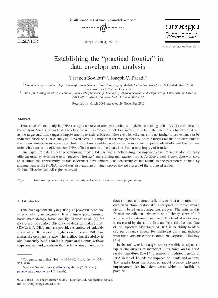
In this paper an upper limit, (1 + �), is considered in theP-DEA model for the e6ciency of the new unit otherwisethe model would be unbounded. The amount of possible in-crease in the e6ciency of an empirically e6cient unit, des-ignated as �, can be speci8ed by management (for exam-ple: 5%). This is an estimate and does not mean that thee6ciency improvement for all e6cient units will necessar-ily be 5%. Based on the P-DEA model’s results, for someunits it will be more or less than 5% while for some otherunits there might be no improvements possible and that isthe reason for the practical frontier “touching” the empiricalone, see Figure 1, which shows the theoretical, practical andempirical frontiers for the case of one input and one out-put. In this 8gure the curve shows the theoretical frontier,which of course is unknown in any analysis where humanperformance is studied.

The upper and lower bounds for factors and the possibleimprove in e6ciency of an empirically e6cient unit (�) canbe local or global (the same for all units) based on the appli-

2 Although, inputs and outputs are not known and speci8edbounds based on management opinion are used in this model, it isdiMerent from an IDEA model. The IDEA model is used to mea-sure the relative e6ciency of decision making units when the valuefor some (all) inputs and outputs is unknown, having bounded datais one example of imprecise data. The proposed model is used tocreate an improved unit and to ensure that, the e6ciency of theunit under consideration is set to be greater or equal to 1.0. Thismodel must be run for each e6cient unit.

0123456789

0 5 10 15

Empirical Practical

Fig. 1. The theoretical, practical and empirical frontiers.

cation; for example for comparing diMerent branches of thesame bank the information can be global, while it can be lo-cal if diMerent banks are compared. Acquiring managementinput regarding the performance of one real DMU at a timeoMers a great advantage according to [14], since it needs tohave local rather than global validity.

The P-DEA ratio model, (2), can be transformed into alinear fractional programming model by substituting y r0urand xi0vi with new variables pr and qi, respectively, andreplacing Lxi0 6 xi06Uxi0 and Lyr0 6 y r06Uyr0 withviLxi0 6 qi6 viUxi0 and urLyr0 6pr6 urUyr0 , correspond-ingly. Then the linear fractional program can be transformedto a linear program [15], which is shown in (3), so thatthe linear programming method can be applied to solve thecase. The process is relatively straightforward.

Maxs∑

r=1

pr + u0

s:t:m∑

i=1

qi = 1;

s∑

r=1

yrjur + u0 −m∑

i=1

xijvi6 0; ∀j;

s∑

r=1

pr + u0 −m∑

i=1

qi¿ 0;

s∑

r=1

pr + u0 −m∑

i=1

qi(1 + �)6 0;

urLyr0 6pr6 urUyr0 ; ∀r;viLxi0 6 qi6 viUxi0 ; ∀i;ur ; �i¿ ; ∀r; i;u0 free: (3)

By solving the above model, x∗i0 =q∗i =v

∗i and y∗r0 =p

∗r =u

∗r

can be calculated. These values are the inputs and outputsof the arti8cial unit. In order to de8ne the practical frontier,the P-DEA model must be run for each e6cient unit.


DEA Models including

bounded ones

I/O of real units Inefficient units

Management opinion about I/O bounds and the possible increase in efficiency of efficient units ( )

I/O of new units

DEA Model

Practical Frontier

Sta

ge 1

S

tage

2

Sta

ge 3

Efficient Units

Management opinion on weight bounds

Proposed P-DEA model

δ

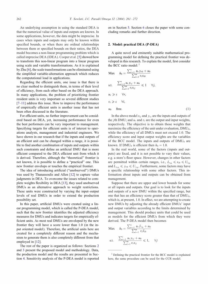
Fig. 2. Methodology.

3. Methodology

The proposed procedure for improving the e6cient unitand 8nding the practical frontier has three stages. Figure 2summarizes the proposed methodology. In the 8rst stage, weevaluate the e6ciency of all real units using conventionalDEAmethodology and 8nd the e6cient and ine6cient units.This 8rst stage may itself comprise of several steps start-ing with an unrestricted DEA run, followed by constrainedmodels until a satisfactory model is developed.

In the second stage, we have to obtain the ranges withinwhich the inputs and outputs of the e6cient units can vary.We chose to obtain the magnitude of the possible improve-ment for already e6cient DMUs by interviewing manage-ment. Then, using this information we solve the proposedP-DEA model for each e6cient unit in order to 8nd theinputs and outputs of the new “improved” DMUs, whichtogether with a few empirical units will form the practicalfrontier.

Finally, in the last stage, we run the DEA model withall the real and new “improved” DMUs together, includingany constraints, de8ning the new frontier. This new frontierenvelops or touches the old one but will not cross it—seeFigure 1 above.

4. Data, analyses and results

4.1. Data

The robustness of the results of a DEA analysis relieson the availability and quality of the data. Our data set,which was a good clean database comprised of bank branchdata, was provided by a large Canadian Bank. It consists

BANK BRANCH

FTE Sales

FTE Support

FTE Other

Loans

Mortgages

RRSPs

Letters of Credit

OUTPUTS: SalesINPUTS: Personnel

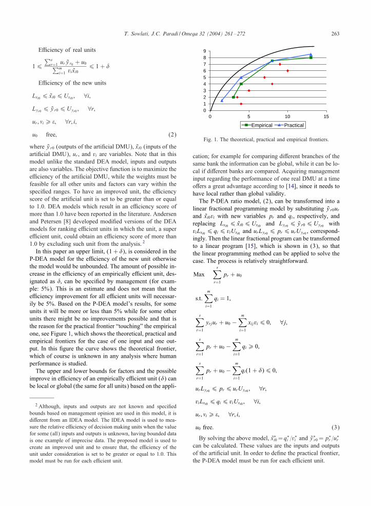
Fig. 3. DEA production model.

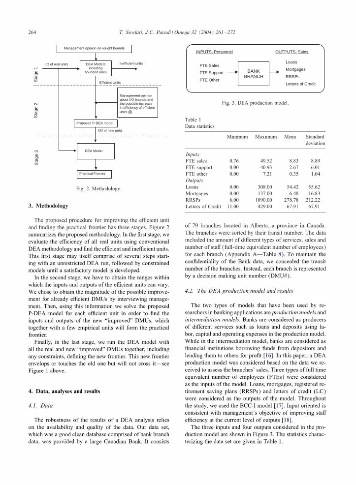
Table 1Data statistics

Minimum Maximum Mean Standarddeviation

InputsFTE sales 0.76 49.52 8.83 8.89FTE support 0.00 40.93 2.67 6.01FTE other 0.00 7.21 0.35 1.04OutputsLoans 0.00 308.00 54.42 55.62Mortgages 0.00 137.00 6.48 16.83RRSPs 6.00 1090.00 278.78 212.22Letters of Credit 11.00 429.00 67.91 67.91

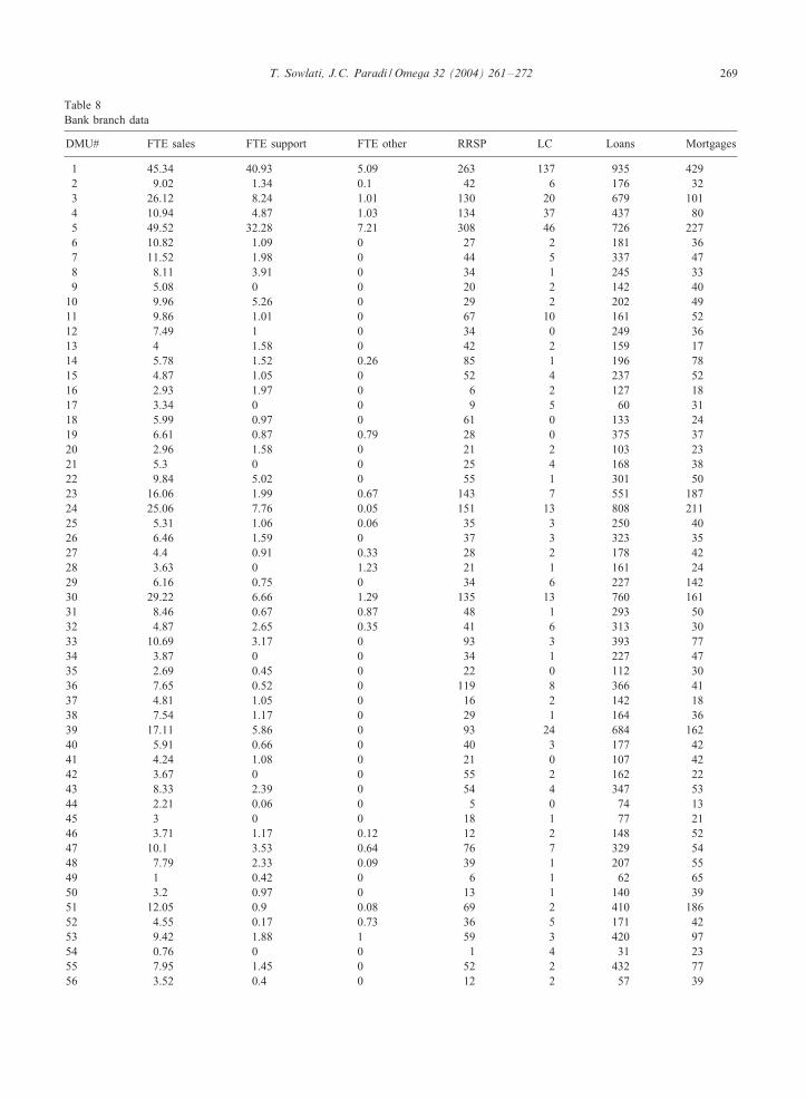
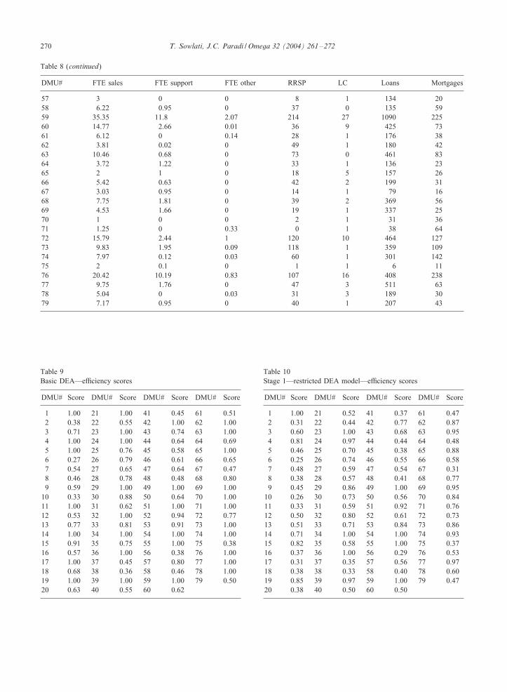
of 79 branches located in Alberta, a province in Canada.The branches were sorted by their transit number. The dataincluded the amount of diMerent types of services, sales andnumber of staM (full-time equivalent number of employees)for each branch (Appendix A—Table 8). To maintain thecon8dentiality of the Bank data, we concealed the transitnumber of the branches. Instead, each branch is representedby a decision making unit number (DMU#).

4.2. The DEA production model and results

The two types of models that have been used by re-searchers in banking applications are production models andintermediation models. Banks are considered as producersof diMerent services such as loans and deposits using la-bor, capital and operating expenses in the production model.While in the intermediation model, banks are considered as8nancial institutions borrowing funds from depositors andlending them to others for pro8t [16]. In this paper, a DEAproduction model was considered based on the data we re-ceived to assess the branches’ sales. Three types of full timeequivalent number of employees (FTEs) were consideredas the inputs of the model. Loans, mortgages, registered re-tirement saving plans (RRSPs) and letters of credit (LC)were considered as the outputs of the model. Throughoutthe study, we used the BCC-I model [17]. Input oriented isconsistent with management’s objective of improving staMe6ciency at the current level of outputs [18].

The three inputs and four outputs considered in the pro-duction model are shown in Figure 3. The statistics charac-terizing the data set are given in Table 1.


The key issues (the size of the sample, the number of in-puts and outputs included in the analysis and the degree ofcorrelation between inputs and outputs) as highlighted byPedraja-Chaparro et al. [19] have a great inOuence on therobustness of the DEA model. Hence, these were analyzedprior to obtaining the branch e6ciency scores. The com-mercial software package DEA-Solver-Pro was used in thiswork. Based on the DEA results, 41% of branches (32 outof 79) were e6cient (Appendix A—Table 9).

4.3. Incorporating management opinion

In the second stage of the methodology, in order to de-velop the arti8cial units, management input is required. Thestrategy we followed here centered on the potential “per-ception” and “credibility” of any suggestion for improve-ment made by this project. Remembering that people do notlike to be measured under the best of circumstances, theylike even less being told to improve when they appear to beamong the best there is. We theorized, and senior manage-ment agreed, that if those in control of the enterprise givetheir best guesses as to what improvement their organiza-tion can achieve, we would have a more positive reception.Hence, a meeting with the Bank’s VPs was set and a ques-tionnaire was prepared. It was a structured meeting and themain questions were about their opinion and judgement on:

• The production model constructed—should we consideradding or deleting any input or output variables?

• The importance of each input and output—do the vari-ables have the same weight?

• The e6ciency of the best practice branches—can it be in-creased? How much of an increase would be reasonable?

• The inputs and/or outputs—are they 8xed? Can they bechanged?

• Allowable changes (a range of + or −)—Is it the samemagnitude for all branches or can changes be variable withrespect to diMerent groups (type of branch, urban-rural)?

Two VPs participated in the questionnaire and they dis-cussed it together prior to returning it. Their perspective tothe questions were as follows:

• Production model: It was suggested to include revenueas the output of the model rather than sales’ volume tohave a stronger decision making tool. However, reliabledata was not available in the quantities required, so thiswas not implemented.

• Weighting: In terms of inputs they suggested to weightthem as follows: FTE sales—50%, FTE support—30%,FTE other—20%. The following weighting could beapplied to the outputs: loans, mortgages, RRSPs—30%each, and letters of credit—10%.

• E9ciency score of the best practice branches: They feltthat a 2–4% increase in e6ciency would be a realisticexpectation on an annual basis.

Table 2E6ciency results—comparison

Model # DMUs % E6cient Minimum Averageunits e6ciency e6ciency

score score

Basic DEA 79—real 41 0.27 0.77Restricted DEA 79—real 10 0.25 0.64

• Inputs/outputs: All inputs and outputs should be able tobe changed.

• Allowable ranges: For inputs, no more than 5% increaseand 20% decrease would be allowable. For outputs: theywould set the increase to no more than 50% and the de-crease to no more than 10%.

• No groupings were identi8ed based on branch size.

4.4. The restricted DEA model

In the basic DEA model discussed so far, the weightswere allowed to vary freely and this Oexibility made the unitappear at its best; however, based on management opinionthe model could be more realistic considering the relativeimportance of the weights. Such concept was expressed aspercentages by management. They were converted to con-straints as ratios and then added to the basic model to geta re8ned measure of e6ciency. The mathematical form ofthese constraints are shown below:

�2(FTE support)

�1(FTE sales)=

35;

�3(FTE other)

�1(FTE sales)=

25;

u3(Loans)u1(RRSPs)

= 1;

u4(Mortgages)

u1(RRSPs)= 1;

u2(Letters of credit)

u1(RRSPs)=

13: (4)

These constraints were added to the basic DEA modeland the assurance region model (AR-I-V) was solved us-ing DEA-Solver-PRO software. The e6ciency results of thebasic model and the restricted model are summarized andcompared in Table 2. The e6ciency scores of the restrictedmodel are given in Appendix A—Table 10.

Although the minimum e6ciency score in the restrictedmodel has not changed much when compared to the ba-sic model, the number of e6cient branches has decreasedsigni8cantly as only 10% of the units (8 branches out of79) remained e6cient. Adding the weight constraints to theDEA model increased the discriminating power of DEA, asexpected.


Table 3Stage 2—inputs and outputs of arti8cial units

DMU# FTE sales FTE support FTE other RRSP LC Loans Mortgages

80 36.27 32.74 4.07 236.70 123.30 841.50 496.6081 16.27 2.09 0.70 128.70 10.50 495.90 280.5082 4.06 0.00 0.00 30.60 0.90 290.45 70.5083 8.03 0.55 0.00 107.10 12.00 486.23 61.5084 1.05 0.44 0.00 9.00 1.50 93.00 97.5085 0.61 0.00 0.00 1.50 6.00 46.50 34.5086 8.35 1.52 0.00 46.80 3.00 565.56 69.3087 28.28 9.44 1.66 192.60 24.30 981.00 202.50

Table 4E6ciency results—8rst and third stage comparison

Model Restricted DEA (Stage 1) Restricted DEA (Stage 3)

# DMUs 79-real 87-real and arti8cial% E6cient units 10 9Minimum e6ciency score 0.25 0.17Average e6ciency score 0.64 0.52#Arti8cial units on the frontier — 6#Arti8cial units not on the frontier but improved — 2#Real units on the frontier — 2

To detect the possibility of having outliers and theirinOuence on the DEA e6ciency measures, we developedseveral DEA restricted models by removing one e6-cient DMU at a time. Outliers are atypical observationsand, in most analyses, these should be deleted from thedata set, for example having commercial branches in thedata set which form the e6cient frontier but their oper-ations are completely diMerent from other branches. Todeal with the problem of outliers in DEA, the e6cientobservations can be deleted until e6ciency estimates sta-bilized [20]. Since the alternative models produced similarand stable results, the possibility of having outliers waseliminated.

4.5. Creating new units—stage 2

Once management opinion was acquired, it was possibleto replace the required parameters in our model and 8nd theinputs and outputs of the arti8cial units. These parameterswere: possible increase in e6ciency of the best practiceunits (�); input and output allowable ranges of variation(Lxi0 6 xi06Uxi0 , Lyr0 6 y r06Uyr0 ). Eq. (5) shows thedesired replacements:

�= 0:04;

(1− 0:20)∗xi06 xi06 (1 + 0:05)∗xi0; ∀i;

(1− 0:10)∗yr06 y r06 (1 + 0:50)∗yr0; ∀j: (5)

Then, the proposed P-DEA model was solved for each ef-8cient unit, which has scored 1.0 in the 8rst stage-DEA anal-ysis (DEA with restricted weights), using Excel’s Solver.The same weight constraints as Stage1 were also used here.The inputs and outputs of 8 new units were found and areshown in Table 3.

4.6. Establishing the practical frontier—stage 3

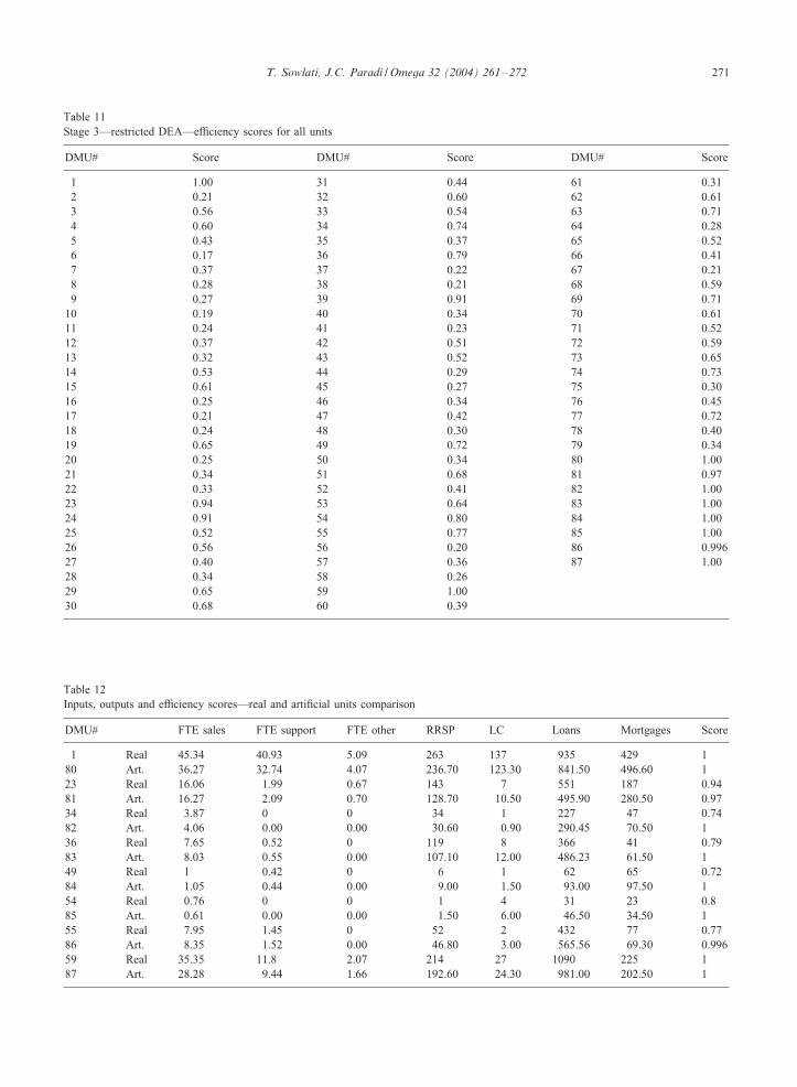
In the last stage, the DEA-Solver-PRO software was usedto solve the production model for the 79 real branches andeight arti8cial units altogether considering the same weightrestrictions as stages 1 and 2. The e6ciency scores of theunits are given in Appendix A—Table 11. The e6ciencyresults of the models in stages 1 and 3 are compared inTable 4.

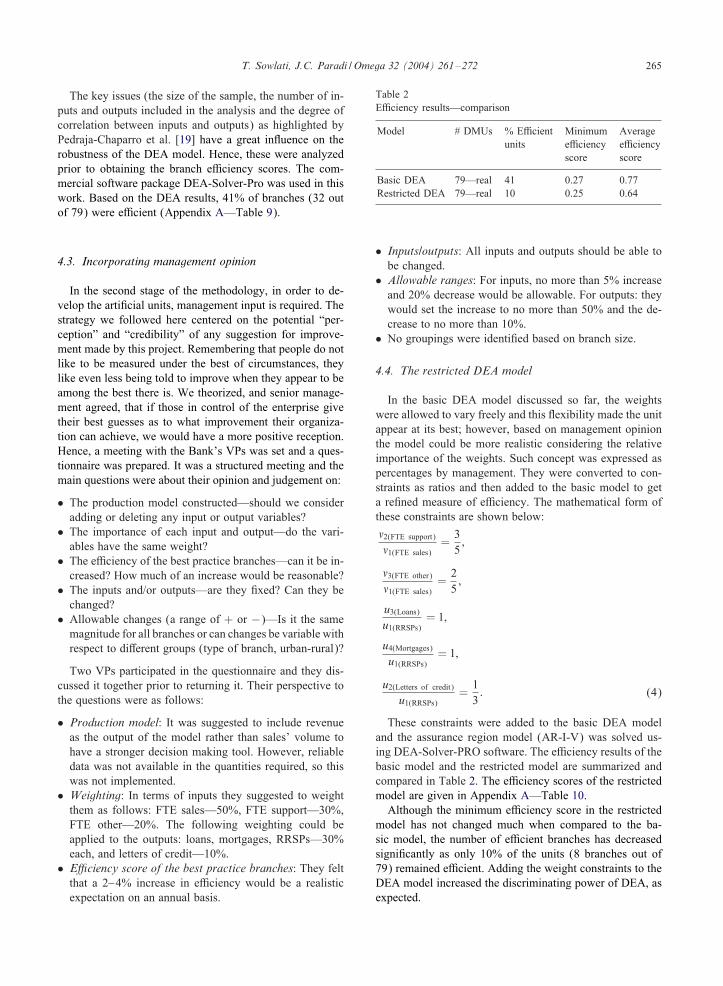
The comparison of the e6ciency score distribution of theDEAmodel from Stages 1 and 3 is presented in Figure 4. Thenumber of units in the analysis of Stage 3 has increased com-pared to Stage 1 thus increasing the discriminating power ofDEA. This can be noticed in Table 4 where the % e6cientunits, the average and the minimum e6ciency scores of themodel in Stage 3 have decreased compared to those of themodel in Stage 1.

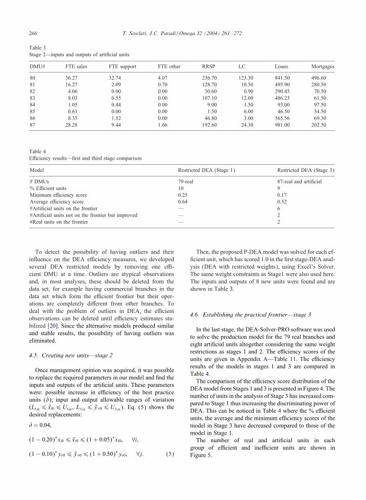
The number of real and arti8cial units in eachgroup of e6cient and ine6cient units are shown inFigure 5.


0

5

10

15

20

0 0.1 0.2 0.3 0.4 0.5 0.6 0.7 0.8 0.9 1

Fre

quen

cy o

f Occ

uran

ce

Stage3

Stage1

Efficiency Score Distribution- Comparison

Efficiency Score

Fig. 4. E6ciency score distribution—Stages 1 and 3.

Efficient and Inefficient Group

0

10

20

30

40

50

60

70

80

90

Efficient Units Inefficient Units

Num

ber

of U

nits

Real

Artificial

Fig. 5. Number of real and arti8cial units in each group.

As it is shown in Figure 5, all the units on the new fron-tier (8 e6cient units) are either real units (2) or arti8cialunits found in stage two (6). For those real units which arestill on the frontier no further improvement is indicated bythis study. This could mean that these two units are trulye6cient as they can respond to the increased performanceand operating environment and still stay e6cient. It can alsomean that the size of � is too small to make any diMerenceto these DMUs.

Table 5 shows the inputs and outputs (I/O) of an arti8cialunit (DMU# 81), its source unit (DMU# 23) and the upperand lower bounds for each factor. Using the P-DEA model,an arti8cial unit is created with another combination of I/Othat is more e6cient than its source unit. As it was expected,

Table 5Inputs and outputs comparison

DMU# FTE sales FTE support FTE other RRSP LC Loans Mortgages Score

23 (Real) 16.06 1.99 0.67 143 7 551 187 0.9481 (Arti8cial) 16.27 2.09 0.70 128.70 10.5 495.9 280.5 0.97Lower bound 12.85 1.59 0.54 128 6 495 168Upper Bound 16.89 2.09 0.70 215 11 827 281

Third Stage Result

0123456789

Artificial Units

Num

ber

of U

nits

Improved

On the frontier

Fig. 6. Third stage result for arti8cial units.

the I/O are within the upper and lower bounds; and themodel did not set all inputs to lower bounds nor all outputsto upper bounds.

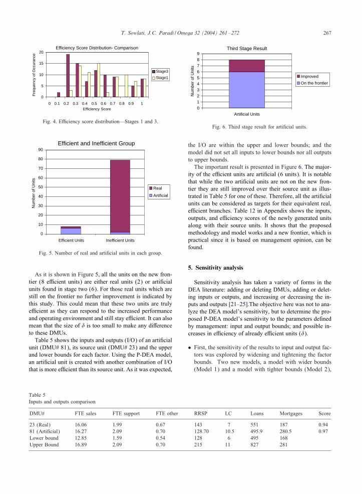
The important result is presented in Figure 6. The major-ity of the e6cient units are arti8cial (6 units). It is notablethat while the two arti8cial units are not on the new fron-tier they are still improved over their source unit as illus-trated in Table 5 for one of these. Therefore, all the arti8cialunits can be considered as targets for their equivalent real,e6cient branches. Table 12 in Appendix shows the inputs,outputs, and e6ciency scores of the newly generated unitsalong with their source units. It shows that the proposedmethodology and model works and a new frontier, which ispractical since it is based on management opinion, can befound.

5. Sensitivity analysis

Sensitivity analysis has taken a variety of forms in theDEA literature: adding or deleting DMUs, adding or delet-ing inputs or outputs, and increasing or decreasing the in-puts and outputs [21–25].The objective here was not to ana-lyze the DEA model’s sensitivity, but to determine the pro-posed P-DEA model’s sensitivity to the parameters de8nedby management: input and output bounds; and possible in-creases in e6ciency of already e6cient units (�).

• First, the sensitivity of the results to input and output fac-tors was explored by widening and tightening the factorbounds. Two new models, a model with wider bounds(Model 1) and a model with tighter bounds (Model 2),


Table 6Summary of results—changing the input and output bounds

Model in Stage 2 P-DEA Original P-DEA Wider P-DEA Tighter boundsbounds for I/O bounds for I/O (Model 1) for I/O (Model 2)

Model in Stage 3 Restricted DEA Restricted DEA Restricted DEA# DMUs 87 87 87

(real + arti8cial) (real + arti8cial) (real + arti8cial)% E6cient units 9 9 6Minimum e6ciency score 0.170 0.164 0.169Average e6ciency score 0.524 0.515 0.50# Arti8cial units on the new frontier 6 6 5# Arti8cial units not on the frontier but improved 2 2 3# Real units on the new frontier 2 2 1

Table 7Summary of results—changing the value of �

Model in Stage 2 P-DEA � = 4% (original) P-DEA � = 6% P-DEA � = 2%

Model in Stage 3 Restricted DEA Restricted DEA Restricted DEA# DMUs 87 87 87

(real + arti8cial) (real + arti8cial) (real + arti8cial)% E6cient units 9 9 9Minimum e6ciency score 0.170 0.160 0.164Average e6ciency score 0.524 0.505 0.514#Arti8cial units on the new frontier 6 6 6# Arti8cial units not on the frontier but improved 2 2 2# Real units on the new frontier 2 2 2

were developed and two sets of arti8cial units were gen-erated. Two new frontiers were established based on thetwo sets of arti8cial units and compared to the frontiercreated from the arti8cial units of the model with the orig-inal bounds.

• The second part of the sensitivity analysis was to investi-gate changes in the � value. The P-DEAmodel was solvedwith diMerent values of �, new sets of units were createdand new frontiers were established.

Tables 6 and Table 7 summarizes the results of changingthe factor bounds and the � value, respectively. It was foundthat the arti8cial units generated from eachmodel were eitheron the new frontier or improved from their source DMUs,hence we have proven the robustness of the proposed P-DEAmodel.

6. Conclusion and further direction

Our research points to the possibility of using a new DEAmodel that provides targets for empirically e6cient units byintroducing new mathematical models that can yield a newfrontier. This new frontier is created using an arbitrary dis-

turbance to the observed inputs and outputs of empiricallye6cient DMUs. This technology accommodates the inclu-sion of managerial input into the P-DEA model by usingtheir know-how in the creation of the disturbances men-tioned above. Since the value of the parameters in the modelcan be acquired from management, this ensures that targetsfor e6cient units are both practical and likely to be fair andequitable from the viewpoints of the staM in the DMUs be-ing measured.

In some applications when management needs to choosethe best project from a group of e6cient projects; or choosea number of e6cient projects based on a limited budget, aform of ranking for the e6cient units can be derived us-ing this method. This new P-DEA approach also providesadjusted e6ciency scores for all units, which may be use-ful in a new ranking process for the best practice units.To investigate this possibility, further research needs to bedone.

Appendix A

Data, Analyses and results are shown in Tables 8–12


Table 8Bank branch data


1 45.34 40.93 5.09 263 137 935 4292 9.02 1.34 0.1 42 6 176 323 26.12 8.24 1.01 130 20 679 1014 10.94 4.87 1.03 134 37 437 805 49.52 32.28 7.21 308 46 726 2276 10.82 1.09 0 27 2 181 367 11.52 1.98 0 44 5 337 478 8.11 3.91 0 34 1 245 339 5.08 0 0 20 2 142 40

10 9.96 5.26 0 29 2 202 4911 9.86 1.01 0 67 10 161 5212 7.49 1 0 34 0 249 3613 4 1.58 0 42 2 159 1714 5.78 1.52 0.26 85 1 196 7815 4.87 1.05 0 52 4 237 5216 2.93 1.97 0 6 2 127 1817 3.34 0 0 9 5 60 3118 5.99 0.97 0 61 0 133 2419 6.61 0.87 0.79 28 0 375 3720 2.96 1.58 0 21 2 103 2321 5.3 0 0 25 4 168 3822 9.84 5.02 0 55 1 301 5023 16.06 1.99 0.67 143 7 551 18724 25.06 7.76 0.05 151 13 808 21125 5.31 1.06 0.06 35 3 250 4026 6.46 1.59 0 37 3 323 3527 4.4 0.91 0.33 28 2 178 4228 3.63 0 1.23 21 1 161 2429 6.16 0.75 0 34 6 227 14230 29.22 6.66 1.29 135 13 760 16131 8.46 0.67 0.87 48 1 293 5032 4.87 2.65 0.35 41 6 313 3033 10.69 3.17 0 93 3 393 7734 3.87 0 0 34 1 227 4735 2.69 0.45 0 22 0 112 3036 7.65 0.52 0 119 8 366 4137 4.81 1.05 0 16 2 142 1838 7.54 1.17 0 29 1 164 3639 17.11 5.86 0 93 24 684 16240 5.91 0.66 0 40 3 177 4241 4.24 1.08 0 21 0 107 4242 3.67 0 0 55 2 162 2243 8.33 2.39 0 54 4 347 5344 2.21 0.06 0 5 0 74 1345 3 0 0 18 1 77 2146 3.71 1.17 0.12 12 2 148 5247 10.1 3.53 0.64 76 7 329 5448 7.79 2.33 0.09 39 1 207 5549 1 0.42 0 6 1 62 6550 3.2 0.97 0 13 1 140 3951 12.05 0.9 0.08 69 2 410 18652 4.55 0.17 0.73 36 5 171 4253 9.42 1.88 1 59 3 420 9754 0.76 0 0 1 4 31 2355 7.95 1.45 0 52 2 432 7756 3.52 0.4 0 12 2 57 39


Table 8 (continued)


57 3 0 0 8 1 134 2058 6.22 0.95 0 37 0 135 5959 35.35 11.8 2.07 214 27 1090 22560 14.77 2.66 0.01 36 9 425 7361 6.12 0 0.14 28 1 176 3862 3.81 0.02 0 49 1 180 4263 10.46 0.68 0 73 0 461 8364 3.72 1.22 0 33 1 136 2365 2 1 0 18 5 157 2666 5.42 0.63 0 42 2 199 3167 3.03 0.95 0 14 1 79 1668 7.75 1.81 0 39 2 369 5669 4.53 1.66 0 19 1 337 2570 1 0 0 2 1 31 3671 1.25 0 0.33 0 1 38 6472 15.79 2.44 1 120 10 464 12773 9.83 1.95 0.09 118 1 359 10974 7.97 0.12 0.03 60 1 301 14275 2 0.1 0 1 1 6 1176 20.42 10.19 0.83 107 16 408 23877 9.75 1.76 0 47 3 511 6378 5.04 0 0.03 31 3 189 3079 7.17 0.95 0 40 1 207 43

Table 9Basic DEA—e6ciency scores

DMU# Score DMU# Score DMU# Score DMU# Score

1 1.00 21 1.00 41 0.45 61 0.512 0.38 22 0.55 42 1.00 62 1.003 0.71 23 1.00 43 0.74 63 1.004 1.00 24 1.00 44 0.64 64 0.695 1.00 25 0.76 45 0.58 65 1.006 0.27 26 0.79 46 0.61 66 0.657 0.54 27 0.65 47 0.64 67 0.478 0.46 28 0.78 48 0.48 68 0.809 0.59 29 1.00 49 1.00 69 1.00

10 0.33 30 0.88 50 0.64 70 1.0011 1.00 31 0.62 51 1.00 71 1.0012 0.53 32 1.00 52 0.94 72 0.7713 0.77 33 0.81 53 0.91 73 1.0014 1.00 34 1.00 54 1.00 74 1.0015 0.91 35 0.75 55 1.00 75 0.3816 0.57 36 1.00 56 0.38 76 1.0017 1.00 37 0.45 57 0.80 77 1.0018 0.68 38 0.36 58 0.46 78 1.0019 1.00 39 1.00 59 1.00 79 0.5020 0.63 40 0.55 60 0.62

Table 10Stage 1—restricted DEA model—e6ciency scores

DMU# Score DMU# Score DMU# Score DMU# Score

1 1.00 21 0.52 41 0.37 61 0.472 0.31 22 0.44 42 0.77 62 0.873 0.60 23 1.00 43 0.68 63 0.954 0.81 24 0.97 44 0.44 64 0.485 0.46 25 0.70 45 0.38 65 0.886 0.25 26 0.74 46 0.55 66 0.587 0.48 27 0.59 47 0.54 67 0.318 0.38 28 0.57 48 0.41 68 0.779 0.45 29 0.86 49 1.00 69 0.95

10 0.26 30 0.73 50 0.56 70 0.8411 0.33 31 0.59 51 0.92 71 0.7612 0.50 32 0.80 52 0.61 72 0.7313 0.51 33 0.71 53 0.84 73 0.8614 0.71 34 1.00 54 1.00 74 0.9315 0.82 35 0.58 55 1.00 75 0.3716 0.37 36 1.00 56 0.29 76 0.5317 0.31 37 0.35 57 0.56 77 0.9718 0.38 38 0.33 58 0.40 78 0.6019 0.85 39 0.97 59 1.00 79 0.4720 0.38 40 0.50 60 0.50


Table 11Stage 3—restricted DEA—e6ciency scores for all units

DMU# Score DMU# Score DMU# Score

1 1.00 31 0.44 61 0.312 0.21 32 0.60 62 0.613 0.56 33 0.54 63 0.714 0.60 34 0.74 64 0.285 0.43 35 0.37 65 0.526 0.17 36 0.79 66 0.417 0.37 37 0.22 67 0.218 0.28 38 0.21 68 0.599 0.27 39 0.91 69 0.71

10 0.19 40 0.34 70 0.6111 0.24 41 0.23 71 0.5212 0.37 42 0.51 72 0.5913 0.32 43 0.52 73 0.6514 0.53 44 0.29 74 0.7315 0.61 45 0.27 75 0.3016 0.25 46 0.34 76 0.4517 0.21 47 0.42 77 0.7218 0.24 48 0.30 78 0.4019 0.65 49 0.72 79 0.3420 0.25 50 0.34 80 1.0021 0.34 51 0.68 81 0.9722 0.33 52 0.41 82 1.0023 0.94 53 0.64 83 1.0024 0.91 54 0.80 84 1.0025 0.52 55 0.77 85 1.0026 0.56 56 0.20 86 0.99627 0.40 57 0.36 87 1.0028 0.34 58 0.2629 0.65 59 1.0030 0.68 60 0.39

Table 12Inputs, outputs and e6ciency scores—real and arti8cial units comparison

DMU# FTE sales FTE support FTE other RRSP LC Loans Mortgages Score

1 Real 45.34 40.93 5.09 263 137 935 429 180 Art. 36.27 32.74 4.07 236.70 123.30 841.50 496.60 123 Real 16.06 1.99 0.67 143 7 551 187 0.9481 Art. 16.27 2.09 0.70 128.70 10.50 495.90 280.50 0.9734 Real 3.87 0 0 34 1 227 47 0.7482 Art. 4.06 0.00 0.00 30.60 0.90 290.45 70.50 136 Real 7.65 0.52 0 119 8 366 41 0.7983 Art. 8.03 0.55 0.00 107.10 12.00 486.23 61.50 149 Real 1 0.42 0 6 1 62 65 0.7284 Art. 1.05 0.44 0.00 9.00 1.50 93.00 97.50 154 Real 0.76 0 0 1 4 31 23 0.885 Art. 0.61 0.00 0.00 1.50 6.00 46.50 34.50 155 Real 7.95 1.45 0 52 2 432 77 0.7786 Art. 8.35 1.52 0.00 46.80 3.00 565.56 69.30 0.99659 Real 35.35 11.8 2.07 214 27 1090 225 187 Art. 28.28 9.44 1.66 192.60 24.30 981.00 202.50 1


References

[1] Charnes A, Cooper WW, Rhodes E. Measuring the e6ciencyof the decision making units. European Journal of OperationalResearch 1978;2(6):429–44.

[2] Charnes A, Cooper WW, Lewin AY, Seiford LM. Dataenvelopment analysis: theory, methodology and applications.Dordrecht: Kluwer Academic Publisher; 1997.

[3] Cooper WW, Seiford LM, Tone K. Data envelopmentanalysis—a comprehensive text with models, applications,references and DEA-solver software. Dordrecht: KluwerAcademic Publisher; 2000.

[4] Kao C. E6ciency improvement in data envelopment analysis.European Journal of Operational Research 1994;73:487–94.

[5] Cooper WW, Park KS, Yu G. IDEA and AR-IDEA: modelsfor dealing with imprecise data in DEA. Management Science1999;45(4):597–607.

[6] Zhu J. Imprecise data envelopment analysis: a reviewand improvement with an application. European Journal ofOperational Research 2003;144:513–29.

[7] Cook WD, Kress M, Seiford LM. Prioritization models forfrontier decision making units in DEA. European Journal ofOperational Research 1992;59:319–23.

[8] Andersen P, Petersen NC. A procedure for ranking e6cientunits in data envelopment analysis. Management Science1993;39(10):1261–4.

[9] Torgersen AM, Forsund FR, Kittelsen SAC. Slack-adjustede6ciency measures and ranking e6cient units. The Journalof Productivity Analysis 1997;7:379–98.

[10] Sinuany-Stern Z, Friedman L. DEA and the discriminantanalysis of ratios for ranking units. European Journal ofOperational Research 1998;111:470–8.

[11] Friedman L, Sinuany-Stern Z. Combining ranking scalesand selecting variables in the DEA context: the case ofindustrial branches. Computers and Operations Research1998;25(2):781–91.

[12] Thanassoulis E, Allen R. Simulating weights restrictions indata envelopment analysis by means of unobserved DMUs.Management Science 1998;44(4):586–94.

[13] Roll Y, Cook WW, Golany B. Controlling factor weights indata envelopment analysis. IIE Transactions 1991;23(1):2–9.

[14] Allen R, Athanassopoulos A, Dyson RG, Thanassoulis E.Weights restrictions and value judgments in data envelopmentanalysis: evolution, development and further directions.Annals of Operations Research 1997;73:13–34.

[15] Charnes A, Cooper WW. Programming with linear fractionals.Naval Research Logistics Quarterly 1962;9(3,4):181–5.

[16] Asmild M, Paradi JC, Aggarwall V, SchaMnit C. CombiningDEA Window Analysis with the Malmquist Index Approachin a Study of the Canadian Banking Industry. The Journal ofProductivity Analysis 2004;21:67–89.

[17] Banker RD, Charnes A, Cooper WW. Some models forestimating technical and scale ine6ciency in data envelopmentanalysis. Management Science 1984;31(9):1078–92.

[18] SchaMnit C, Rosen D, Paradi JC. Best practice analysis of bankbranches: an application of DEA in a large Canadian bank.European Journal of Operational Research 1997;98:269–89.

[19] Pedraja-Chaparro F, Salinas-Jimenez J, Smith P. On thequality of data envelopment analysis. Journal of OperationalResearch Society 1999;50:636–44.

[20] Wilson PW. Detecting outliers in deterministic nonparametricfrontier models with multiple outputs. Journal of Business andEconomic Statistics 1993;11(3):319–23.

[21] Charnes A, Cooper WW, Lewin AY, Morey RC, Rousseau J.Sensitivity and stability analysis in DEA. Annals of OperationsResearch 1985;2:139–56.

[22] Charnes A, Neralic L. Sensitivity analysis of the additivemodel in data envelopment analysis. European Journal ofOperational Research 1990;48:332–41.

[23] Zhu J. Robustness of the e6cient DMUs in dataenvelopment analysis. European Journal of OperationalResearch 1996;90:451–60.

[24] Seiford LM, Zhu J. Stability regions for maintaining e6ciencyin data envelopment analysis. European Journal of OperationalResearch 1998;108:127–39.

[25] Seiford LM, Zhu J. Sensitivity analysis of DEA models forsimultaneous changes in all the data. Journal of the OperationalResearch Society 1998;49:1060–71.

establishing the “practical frontier” in data envelopment analysis

Documents