The London School of Economics and Political Science

Essays on Information Asymmetry in Financial

Market

Shiyang Huang

A thesis submitted to the Department of Finance of the London School

of Economics for the degree of Doctor of Philosophy, London.

September 2014

1

Declaration

I certify that the thesis I have presented for examination for the MPhil/PhD degree of the

London School of Economics and Political Science is solely my own work other than where

I have clearly indicated that it is the work of others (in which case the extent of any work

carried out jointly by me and any other person is clearly identified in it).

The copyright of this thesis rests with the author. Quotation from it is permitted, provided

that full acknowledgement is made. This thesis may not be reproduced without the prior

written consent of the author.

I warrant that this authorization does not, to the best of my belief, infringe the rights of

any third party.

Statement of Conjoint Work

I confirm that Chapter 2 ”Investment Waves under Cross Learning” is jointly co-authored with

Mr.Yao Zeng from Economic Department at Harvard University, and I contributed 50% of this

work.

2

Abstract

I study how asymmetric information affects the financial market in three papers. In the

first paper, I study the joint determination of optimal contracts and equilibrium asset prices

in an economy with multiple principal-agent pairs. Principals design optimal contracts that

provide incentives for agents to acquire costly information. With agency problems, the agents’

compensation depends on the accuracy of their forecasts for asset prices and payoffs. Com-

plementarities in information acquisition delegation arise as follows. As more principals hire

agents to acquire information, asset prices become less noisy. Consequently, agents are more

willing to acquire information because they can forecast asset prices more accurately, thus

mitigating agency problems and encouraging other principals to hire agents. This mechanism

can explain many interesting phenomena in markets, including multiple equilibria, herding,

home bias and idiosyncratic volatility comovement.

In the second paper (co-authored with Yao Zeng from Harvard University), we investi-

gate how firms’ cross learning amplifies industry-wide investment waves. Firms’ investment

opportunities have idiosyncratic shocks as well as a common shock, and firms’ asset prices

aggregate speculators’ private information about these two shocks. In investing, each firm

learns from other firms’ prices to make better inference about the common shock. Thus,

a spiral between firms’ higher investment sensitivity to the common shock and speculators’

higher weighting on the common shock emerges. This leads to systematic risks in investment

waves: higher investment and price comovements as well as their higher comovements with the

common shock. Moreover, each firm’s cross learning creates a new pecuniary externalities on

other firms, because it makes other firms’ prices less informative on their idiosyncratic shocks

through speculators’ endogenous over-weighting on the common shock.

In the third model, we study the effect of introducing an options market on investors’

incentive to collect private information in a rational expectation equilibrium model. We show

that an options market has two effects on information acquisition: a negative effect, as options

3

act as substitutes for information, and a positive effect, as informed investors have less need

for options and can earn profits from selling them. When the population of informed investors

is high because of the low information acquisition cost, the supply for options is larger than

the demand, leading to low option prices. Low option prices in turn induce investors to use

options instead of information to reduce risk, while informed investors have little opportunity

to earn profits from selling options to cover their information acquisition cost. Introducing

an options market thus decreases investors’ incentive to acquire information, and the prices of

the underlying assets become less informative, leading to lower prices and higher volatilities.

A dynamic extension of this analysis shows that introducing an options market increases the

price reactions to earnings announcements. However, when the information acquisition cost

is high, the opposite effects arise. Further analysis shows that our results are robust for

more general derivatives. These results provide a potentially unified theory to reconcile the

conflicting empirical findings on the options listing of individual stocks in both the U.S. market

and international markets.

4

Acknowledgements

Firstly, I would like to thank my advisors, Dimitri Vayanos, for guiding me through the

whole PhD life. His continuous encouragement, invaluable guidance and constant support

helped me greatly in completing the dissertation. Moreover, his infectious enthusiasm for

academic life inspires me to insist my academic dream.

Duration the period when I was doing my dissertation, in addition to my advisors, I also

would like to thank Amil Dasgupta, Dong Lou, Christopher Polk, Kathy Yuan, Yao Zeng and

many others for their valuable comments and advice. I also have to thank all participants at

the LSE Finance PhD seminar and lunch-time seminar of Paul Woolley Centre for the Study

of Capital Market Dysfunctionality at LSE, for their very helpful suggestions and comments.

I owe special thanks to my wife, Yuxiao Peng, for her continuous encouragement and

support during my PhD study program. This dissertation is simply impossible without her.

Finally, the funding from LSE Scholarship and the Paul Woolley Centre for the Study of

Capital Market Dysfunctionality at LSE is gratefully acknowledged.

5

Contents

1 Delegated Information Acquisition and Asset Price 12

1.1 Introduction . . . . . . . . . . . . . . . . . . . . . . . . . . . . . . . . . . . . . . 13

1.2 Model . . . . . . . . . . . . . . . . . . . . . . . . . . . . . . . . . . . . . . . . . 19

1.2.1 Economy . . . . . . . . . . . . . . . . . . . . . . . . . . . . . . . . . . . 19

1.2.2 Discussion . . . . . . . . . . . . . . . . . . . . . . . . . . . . . . . . . . . 24

1.3 Equilibrium . . . . . . . . . . . . . . . . . . . . . . . . . . . . . . . . . . . . . . 26

1.3.1 Equilibrium Definition . . . . . . . . . . . . . . . . . . . . . . . . . . . . 26

1.3.2 Equilibrium Characterization . . . . . . . . . . . . . . . . . . . . . . . . 27

1.3.3 Characteristics of Optimal Contract . . . . . . . . . . . . . . . . . . . . 33

1.4 Agency Problem and Information Acquisition Complementarity . . . . . . . . . 34

1.4.1 First-Best Case . . . . . . . . . . . . . . . . . . . . . . . . . . . . . . . . 34

1.4.2 Agency Problem . . . . . . . . . . . . . . . . . . . . . . . . . . . . . . . 35

1.4.3 Multiplicity of Equilibria . . . . . . . . . . . . . . . . . . . . . . . . . . 36

1.5 Implications . . . . . . . . . . . . . . . . . . . . . . . . . . . . . . . . . . . . . . 39

1.5.1 Herding . . . . . . . . . . . . . . . . . . . . . . . . . . . . . . . . . . . . 41

1.5.2 Home/Industry Bias . . . . . . . . . . . . . . . . . . . . . . . . . . . . . 44

6

1.5.3 Idiosyncratic Volatility Comovement . . . . . . . . . . . . . . . . . . . . 47

1.6 Generalization . . . . . . . . . . . . . . . . . . . . . . . . . . . . . . . . . . . . 51

1.6.1 General Utility Function of Agents . . . . . . . . . . . . . . . . . . . . . 51

1.6.2 More General Distribution of V . . . . . . . . . . . . . . . . . . . . . . . 53

1.6.3 Learning . . . . . . . . . . . . . . . . . . . . . . . . . . . . . . . . . . . . 54

1.7 Conclusion . . . . . . . . . . . . . . . . . . . . . . . . . . . . . . . . . . . . . . 61

1.8 Appendix . . . . . . . . . . . . . . . . . . . . . . . . . . . . . . . . . . . . . . . 72

1.8.1 Proofs . . . . . . . . . . . . . . . . . . . . . . . . . . . . . . . . . . . . . 72

2 Investment Waves under Cross Learning 91

2.1 Introduction . . . . . . . . . . . . . . . . . . . . . . . . . . . . . . . . . . . . . . 92

2.2 Model . . . . . . . . . . . . . . . . . . . . . . . . . . . . . . . . . . . . . . . . . 101

2.2.1 Economy . . . . . . . . . . . . . . . . . . . . . . . . . . . . . . . . . . . 101

2.2.2 Capital Providers and Investment . . . . . . . . . . . . . . . . . . . . . 102

2.2.3 Speculators and Secondary Market Trading . . . . . . . . . . . . . . . . 103

2.2.4 Discussion . . . . . . . . . . . . . . . . . . . . . . . . . . . . . . . . . . . 105

2.3 Cross-Learning Equilibrium . . . . . . . . . . . . . . . . . . . . . . . . . . . . . 107

2.3.1 Equilibrium Definition . . . . . . . . . . . . . . . . . . . . . . . . . . . . 107

2.3.2 Equilibrium Characterization . . . . . . . . . . . . . . . . . . . . . . . . 107

2.3.3 Self-Feedback Benchmark . . . . . . . . . . . . . . . . . . . . . . . . . . 113

2.4 Systematic Risks in Investment Waves . . . . . . . . . . . . . . . . . . . . . . . 117

2.4.1 Impacts of Speculators’ Weight on Systematic Risks . . . . . . . . . . . 117

2.4.2 Endogenous Cross Learning and Systematic Risks . . . . . . . . . . . . 119

7

Common Uncertainty . . . . . . . . . . . . . . . . . . . . . . . . . . . . 119

Capital Providers’ Access to Information . . . . . . . . . . . . . . . . . 122

Liquidity Trading . . . . . . . . . . . . . . . . . . . . . . . . . . . . . . . 124

2.5 Investment Inefficiency and Competition . . . . . . . . . . . . . . . . . . . . . . 125

2.5.1 Overall Investment Efficiency . . . . . . . . . . . . . . . . . . . . . . . . 125

2.5.2 Competition and Cross Learning . . . . . . . . . . . . . . . . . . . . . . 128

2.6 Discussion . . . . . . . . . . . . . . . . . . . . . . . . . . . . . . . . . . . . . . . 135

2.6.1 Over-investment under Cross Learning . . . . . . . . . . . . . . . . . . . 135

2.6.2 Industry Momentum under Cross Learning . . . . . . . . . . . . . . . . 137

2.7 Conclusion . . . . . . . . . . . . . . . . . . . . . . . . . . . . . . . . . . . . . . 138

2.8 Appendix . . . . . . . . . . . . . . . . . . . . . . . . . . . . . . . . . . . . . . . 147

2.8.1 Proofs . . . . . . . . . . . . . . . . . . . . . . . . . . . . . . . . . . . . . 147

3 How Options Affect Information Acquisition and Asset Pricing 165

3.1 Introduction . . . . . . . . . . . . . . . . . . . . . . . . . . . . . . . . . . . . . . 167

3.2 Model . . . . . . . . . . . . . . . . . . . . . . . . . . . . . . . . . . . . . . . . . 172

3.2.1 Timeline and assets . . . . . . . . . . . . . . . . . . . . . . . . . . . . . 173

3.2.2 Investors and information acquisition . . . . . . . . . . . . . . . . . . . . 174

3.2.3 Information acquisition without an options market . . . . . . . . . . . . 174

3.3 Introduction of an Option Market . . . . . . . . . . . . . . . . . . . . . . . . . 177

3.4 Dynamic Model with an Options Market . . . . . . . . . . . . . . . . . . . . . . 184

3.4.1 Dynamic model without an Options Market . . . . . . . . . . . . . . . . 184

3.4.2 Dynamic model with an options market . . . . . . . . . . . . . . . . . . 189

8

3.4.3 Effect of additional trading rounds . . . . . . . . . . . . . . . . . . . . . 193

3.5 Discussion . . . . . . . . . . . . . . . . . . . . . . . . . . . . . . . . . . . . . . . 195

3.6 Conclusions . . . . . . . . . . . . . . . . . . . . . . . . . . . . . . . . . . . . . . 197

3.7 Appendix . . . . . . . . . . . . . . . . . . . . . . . . . . . . . . . . . . . . . . . 207

9

List of Figures

1.4.1 Information Acquisition Benefit . . . . . . . . . . . . . . . . . . . . . . . . . . . 38

1.4.2 Population of Informed Principal and Agents’ Risk Aversion . . . . . . . . . . . 40

1.4.3 Population of Informed Principals and Residual Uncertainty . . . . . . . . . . . 40

1.5.1 Noisy Traders in Asset 1 and Population of Informed Principals in Asset 2 . . . 49

1.5.2 Idiosyncratic Volatility Comovement . . . . . . . . . . . . . . . . . . . . . . . . 50

1.5.3 Population of Informed Principals both Asset Markets . . . . . . . . . . . . . . 50

1.6.1 Information Acquisition Benefit: Triple-State Case . . . . . . . . . . . . . . . . 55

1.6.2 Population of Informed Principal and Agents’ Risk Aversion: Triple-State Case 55

1.6.3 Population of Informed Principal and Residual Uncertainty: Triple-State Case 56

1.6.4 Information Acquisition Benefit: Learning Case . . . . . . . . . . . . . . . . . . 61

2.1.1 Self-Feedback Benchmark . . . . . . . . . . . . . . . . . . . . . . . . . . . . . . 94

2.1.2 Firm / Capital Provider Cross Learning . . . . . . . . . . . . . . . . . . . . . . 95

2.4.1 Mechanical Effect on Systematic Risks . . . . . . . . . . . . . . . . . . . . . . . 121

2.4.2 Learning Effect on Systematic Risks . . . . . . . . . . . . . . . . . . . . . . . . 139

2.5.1 Extended Cross-Learning Framework . . . . . . . . . . . . . . . . . . . . . . . . 140

2.5.2 Competition on Cross Learning and Efficiency Loss . . . . . . . . . . . . . . . . 140

10

3.1.1 Trading Activity in the U.S. Options Market (in millions of dollars) . . . . . . 168

3.2.1 The Relationship between the Population of Informed Investors and the Acqui-

sition Cost . . . . . . . . . . . . . . . . . . . . . . . . . . . . . . . . . . . . . . . 176

3.3.1 Gain from Information Acquisition: Effect of an Options Market . . . . . . . . 180

3.3.2 The Relationship Between Population of Informed Investors and Acquisition

Cost: Effect of Option Market . . . . . . . . . . . . . . . . . . . . . . . . . . . . 181

3.5.1 Gain from Information Acquisition: g(y) = y . . . . . . . . . . . . . . . . . . . 198

3.5.2 Gain from Information Acquisition: g(y) = y2 . . . . . . . . . . . . . . . . . . . 198

11

Chapter 1

Delegated Information Acquisition

and Asset Price

Shiyang Huang

Abstract: This paper studies the joint determination of optimal contracts and equilibrium

asset prices in an economy with multiple principal-agent pairs. Principals design optimal con-

tracts that provide incentives for agents to acquire costly information. With agency problems,

the agents’ compensation depends on the accuracy of their forecasts for asset prices and payoffs.

Complementarities in information acquisition delegation arise as follows. As more principals

hire agents to acquire information, asset prices become less noisy. Consequently, agents are

more willing to acquire information because they can forecast asset prices more accurately, thus

mitigating agency problems and encouraging other principals to hire agents. This mechanism

can explain many interesting phenomena in markets, including multiple equilibria, herding,

home bias and idiosyncratic volatility comovement.

12

1.1 Introduction

The asset management industry has experienced tremendous growth with current assets under

management comparable to global GDP. Not surprisingly, institutional investors now dominate

trading activities in all financial markets.1 While institutions assist their clients in making in-

vestment decisions, agency problems may simultaneously arise. In particular, potential moral

hazard emerges when institutions’ efforts are largely unobservable, raising the issue of optimal

contract design. Given institutions’ superior capabilities to acquire information, it is common-

place for clients to delegate information acquisition to them and provide incentives for them

through optimal contracting. However, the joint determination of optimal contracts, informa-

tion acquisition delegation and equilibrium asset pricing has not yet been fully explored in the

literature.2

This paper contributes to the literature by solving for optimal contracts characterized in a

general space and equilibrium asset prices in an economy with multiple principal-agent pairs.

I show that the optimal contracts for delegated information acquisition depend on agents’

forecasting accuracy for asset prices and payoffs: agents receive high compensation when they

produce accurate forecasts. Moreover, I find strategic complementarities in the delegation of

information acquisition: the more principals hire agents to acquire information, the more others

are willing to do so. As more principals hire agents to acquire information, asset prices become

less noisy. As a result, agents are more willing to acquire information because they can forecast

asset prices more accurately. Thus, the agency problems are mitigated and other principals

are encouraged to hire agents. Such strategic complementarities yield multiple equilibria, and

can explain many phenomena, including asset price jumps, herding behaviour, home bias and

1French (2008) documents that financial institutions accounted for more than 80% ownership of equities inthe U.S. in 2007, compared to 50% in 1980. TheCityUK (2013) estimates the size of assets under managementis around $87 trillion globally, which is equal to global GDP. Meanwhile, Jones and Lipson (2004) reports thatinstitutional trading volume reached 96% of total equity trading volume in NYSE by 2002.

2Papers studying optimal contracts without any asset pricing implications include Bhattacharya and Pflei-derer (1985) and Dybvig et al. (2010). Papers studying institutions’ impacts on asset pricing without asymmetricinformation or information acquisition include Vayanos and Woolley (2013) and Basak and Pavlova (2013). Themost relevant papers are by Kyle, Ou-Yang and Wei (2011) and Malamud and Petrov (2014). However, theyonly consider restricted contract space. More importantly, my research has new asset pricing implications, suchas strategic complementarities.

13

idiosyncratic volatility comovement.

The model of this paper features delegated information acquisition, optimal contract de-

sign, and equilibrium asset pricing, introducing a two-period economy with one risky asset and

one risk-free asset. The risky asset’s payoff has two components: the first can be learned by

agents and is called fundamental value, while the other cannot be learned and produces residual

uncertainty. This economy has a market maker, noisy traders and a mass of principal-agent

pairs. The principals are risk neutral while the agents are risk averse. Different principals

cannot share agents, and different agents cannot share principals. Before trading, the princi-

pals choose whether to hire agents to acquire information regarding fundamental value. When

deciding to hire agents, principals design optimal contracts that provide incentives for agents

to acquire costly information, after which agents provide forecasts to their corresponding prin-

cipals. The feasible contracts are general functions of agents’ forecasts, the asset price and the

payoff. I model agency problems by assuming that agents take hidden actions when acquir-

ing information. When the market opens, the principals submit market orders to the market

maker based on agents’ forecasts. Having received all orders from the principals and the noisy

traders, the market maker then sets the price.

The generality of this model relies on its broad interpretations. The principal-agent pairing

can be interpreted as either that between fund managers and in-house analysts, or that between

the pension fund trustees/board of directors (within funds) and fund managers. This model

can unify both, because the optimal contract problems in the two contexts are essentially

equivalent given that agents construct portfolios based on forecasts and principals can directly

observe agents’ portfolios. Therefore, the assumption regarding who invests is not crucial, and

the aforementioned parsimonious model is a natural setting to study information acquisition

incentives.

I show that the optimal contracts depend on the agents’ forecasting accuracy for the as-

set price and the payoff. Agents can forecast the asset price and payoff accurately only if

they acquire information. Thus, the agents’ efforts are related to their forecasting accuracy,

which determines their compensation. Specifically, agents receive high compensation when

14

they forecast accurately - in contrast to an economy without agency problems, in which the

compensation is constant. As an incentive for accurate forecasting, the bonus decreases with

price informativeness and increases with residual uncertainty. When the price becomes more

informative or residual uncertainty decreases, it is easier for agents to use information to fore-

cast accurately and then receive high compensation. Consequently, agents are more willing to

exert efforts and principals can accordingly provide fewer incentives. These results predict that

the bonus is larger for professionals who trade small/growth stocks featuring greater residual

uncertainty.

Furthermore, I find that the delegation of information acquisition exhibits strategic com-

plementarities. Price informativeness has two counteractive effects: the first is to lower trading

profit; and, the second is to mitigate agency problems. Whereas the first effect leads to stan-

dard strategic substitutability due to competition in trading, the strategic complementarities

in information acquisition delegation originates from the effect of price informativeness on mit-

igating agency problems. When more principals hire agents to acquire information, the asset

price becomes less noisy. As a result, agents are more willing to acquire information because

they can forecast the asset price more accurately, and thus agency problems are mitigated.

Clearly, strategic complementarities in information acquisition delegation emerge when price

informativeness has a larger impact on mitigating agency problems than that on lowering trad-

ing profits. This only occurs when the residual uncertainty is large and compensation must

consequently rely largely on agents’ forecasts for the asset price. This mechanism causes prin-

cipals to coordinate information acquisition delegation, therefore introducing the possibility of

multiple equilibria. The multiplicity of equilibria may lead to the economy switching between

low-information and high-information equilibria without any relation to fundamentals, leading

to jumps in asset price and price informativeness.

This model, to my knowledge, is new to the literature to combine optimal contracts char-

acterized in a general space, equilibrium asset pricing and delegated information acquisition.

Meanwhile, it shows that the agency problem in information acquisition delegation is a new

source for strategic complementarities. In particular, my model yields closed-form solutions

15

for both optimal contracts and equilibrium asset pricing. Although this model is intention-

ally stylized to focus on information acquisition delegation, it captures realistic institutional

features. Moreover, it has a number of implications as follows.

The first implication relates to home bias, a long-standing puzzle.3 A plausible explana-

tion is that investors have superior information on home assets. However, Van Nieuwerburgh

and Veldkamp (2009) argue that investors can easily acquire information about other assets,

which could eliminate the information advantage of home investors and mitigate home bias.4

Although investors can freely acquire information, I show that agency problems lead to home

bias: investors tend to acquire more information about assets for which they have an informa-

tion advantage. I extend the model to consider two groups of principals (A and B) and two

risky assets (X and Y ); group A (B) is endowed with private information only about asset X

(Y ). I show that group A has higher incentives to acquire information on asset X relative to

asset Y , and vice versa. Group A can use the endowed information to monitor agents, and thus

group A’s agency problems are less severe when hiring agents to acquire information about

asset X relative to asset Y .5 Consequently, group A is encouraged to hire agents to acquire

information and trade more on asset X. This result is in direct contrast to that of the economy

without agency problems, in which the decreasing marginal benefit of information discourages

group A from acquiring information about asset X. Interpreting group A as home investors

on asset X implies that agency problems can explain home bias.

The mechanism above for home bias can also explain industry bias: investors trade more on

the assets within their expertise. This prediction is consistent with Massa and Simonov (2006),

who document that Swedish investors buy assets highly correlated with their non-financial

3Home bias is well documented by Fama and Poterba (1991), Coval and Moskowitz (1999) and Grinblattand Keloharju (2001). Despite large benefits from international diversification, Fama and Poterba (1991) findthat households invest nearly all of their wealth in domestic assets. For example, they find that U.S householdsinvest around 94% of their equity portfolio in the domestic market, while this number is 82% in the UK.

4Constraint on international capital flow may explain home bias. However, it is not a major concern cur-rently. In particular, the recent studies (Seasholes and Zhu, 2010 and Coval and Moskowitz, 1999) find thathouseholds/fund managers also have a strong home bias in the U.S. market, which suggests this explanation isnot satisfactory.

5Normally, the principals can use their private information in the subjective evaluation of agents. Evenif the private information is not verifiable, some mechanisms, such as reputation concern, could reveal theseinformation.

16

income. Moreover, because endowed information is more valuable in monitoring agents when

the assets have greater residual uncertainty, the home/industry bias is stronger for these assets.

This prediction is consistent with Kang and Stulz (1997) and Coval and Moskowitz (1999),

who find that the home bias of U.S. fund managers is stronger when they trade small stocks.

The next implication relates to herding, defined as any behavioral similarity caused by

interactions amongst individuals (Hirshleifer and Teoh, 2003). I extend the model to assume

that each principal can choose to hire his agent to acquire either an exclusive signal or a common

signal: the former is only accessible to his agent and is conditionally independent of others,

while the latter is accessible to any agent. Under agency problems, I show that principals

herd to acquire the common signal when the residual uncertainty is sufficiently large. Herding

makes the price sensitive to the common signal itself. Thus, agents are willing to obtain the

common signal because this allows them to easily forecast the asset price. In particular, when

the residual uncertainty is large, herding emerges because its impact on mitigating agency

problems is larger than that on lowering trading profit. This result is in clear contrast to that

of the economy without agency problems, in which principals prefer the exclusive signals due

to the substitute effect.

Moreover, my model has additional applications. For example, I show that idiosyncratic

volatility comovement occurs in a multi-asset extension, in which principals incentivize agents

to acquire information on each asset through their forecasting accuracy for the prices of assets

with correlated fundamentals. An increase on one asset’s idiosyncratic volatility, perhaps due

to more noisy traders, discourages information acquisition and consequently leads to higher

idiosyncratic volatilities on other correlated assets.

This paper is related to several strands of the literature. First, it is related to literature

regarding the optimal contracting in delegated portfolio management, such as Bhattacharya

and Pfleiderer (1985), Stoughton (1993), Dybvig, Farnsworth and Carpenter (2010) and Ou-

Yang (2003). However, the asset prices play no roles in the aforementioned contracting work.

My work on the contracting is most related to Dybvig et al. (2010). They study the optimal

contract problem in a complete market, in which the asset price has no informational role;

17

they find that the optimal compensation involves a benchmark. In contrast to their work, I

consider the optimal contracts in general equilibrium and the asset prices play informational

roles. I find that the compensation depends on agents’ forecasting accuracy for the asset prices

and the payoffs.

My paper is also related to recent studies on the institutional investors, such as Basak,

Shaprio and Tepla (2006), Basak, Pavlova and Shaprio (2007, 2008), Basak and Makarov

(2014), Basak and Pavlova (2013), Dasgupta and Prat (2006, 2008), Dasgupta, Prat and Ver-

ardo (2011), Dow and Gorton (1997), He and Krishnamurthy (2012), He and Kondor (2013),

Garcia and Vande (2009), Kaniel and Kondor (2013), Buffa, Vayanos and Woolley (2013), Kyle,

Ou-Yang and Wei (2011) and Malamud and Petrov (2014). In particular, Buffa, Vayanos and

Woolley (2013) study the joint equilibrium determination of optimal contracts and asset prices

in a dynamic and multi-asset model. They focus on how the inefficiency of benchmarking arises

endogenously and amplifies stock market volatility. However, these authors do not model moral

hazard problems in information acquisition. The most relevant works are by Kyle, Ou-Yang

and Wei (2011) and Malamud and Petrov (2014). Kyle, Ou-Yang and Wei (2011) consider a

moral hazard problem between one principal and one agent in the Kyle (1985) model. They

restrict the contract space and solely consider the linear contracts. Furthermore, Malamud and

Petrov (2014) also focus on the restricted contract form, which consists of one proportional fee

and one option-like incentive fee. My model differs from these papers in the following regard.

First, I place no restrictions on the contract space. Second, I find that the agency problems

generate strategic complementarities in information acquisition delegation, which is new to

this literature.

Last, my paper is related to recent studies on the strategic complementarities, including

Dow, Goldstein and Guembel (2011), Froot, Scharfstein and Stein (1992), Garcia and Strobl

(2011) and Veldkamp (2006b). Froot, Scharfstein and Stein (1992) find that short-term in-

vestors herd to acquire similar information. Because they must liquidate assets before payoffs

are realized, the short-term investors can profit on their information only if their informa-

tion is reflected in future prices by the trades of similarly informed investors. Garcia and

18

Strobl (2011) find that relative wealth concern can generate complementarities. Because the

investors’ utilities are negatively affected by others, they tend to hedge others’ impacts by

following others’ information acquisition decision. Dow, Goldstein and Guembel (2011) show

that information acquisition complementarities emerge when the asset prices affect the firms’

investments. Veldkamp (2006b) finds that when the information production has a scale effect,

the selling price of information decreases as more investors buy information. In contrast to

their work, the strategic complementarities in my model originates from the effect of price

informativeness on mitigating agency problems in delegated information acquisition.

The paper is organized as follows. I introduce the model in Section 2 and solve the optimal

contracts in Section 3. Section 4 shows the strategic complementarities and multiple equilibria.

Section 5 studies three applications. Section 6 discusses the robustness. In particular, I solve

a fully-fledged model with non-linear REE to show that the main results are robust in Section

6. Section 7 concludes.

1.2 Model

1.2.1 Economy

My model is built on Kyle (1985), in which investors submit market orders and a market maker

sets the price according to the total order. My model deviates from Kyle (1985) in the following

features: there are a mass of investors and each one has trading constraints.6 Investors in my

model trade in a competitive market, and no single individual investor has any price impact.

My economy has a mass of principal-agent pairs. The principals trade the risky asset

and have incentives to acquire information for profits. However, these principals are unable

to acquire information alone, perhaps because of large information acquisition or opportunity

costs. Before trading, principals choose whether to hire agents to acquire information. Because

agents’ efforts are unobservable, a moral hazard problem arises within each pair. When deciding

6The assumptions of a mass of investors in which each one has trading constraints is not new (see Dow,Goldstein and Guembel, 2011, Goldstein, Ozdenoren and Yuan, 2013 and Malamud and Petrov, 2014).

19

to hire agents, principals design optimal contracts that provide incentives for agents to acquire

information. In particular, the population of principals who hire agents is endogenous in

my model. My analysis of optimal contracting is similar to that of Dybvig et al. (2010). In

particular, I solve optimal contracts without any restriction on the contract space. The optimal

contracts will induce agents to make costly efforts and truthfully report signals.

Timeline and Assets. My economy has three periods t = 0, 1, 2 and two assets. The

first asset is risk-free and the second is risky. The risk-free asset is in zero supply and pays

off one unit of consumption good without uncertainty at time t = 2. The payoff of the risky

asset is denoted by D with two components: V and ε. V and ε are independent. I call V

the fundamental value and ε the residual uncertainty. I assume that V depends on equally

likely states, h and l, realized at time t = 2. V takes Vω (where ω ∈ {h, l}). Without a loss

of generality, I assume that Vh = θ and Vl = −θ, where θ > 0. The residual uncertainty ε is

uniformly distributed on [−M,M ], where M > 0.7 At time t = 0, principals choose whether

to delegate information acquisition to agents. When deciding to hire agents, principals write

contracts with their agents. The contract is denoted by π. Otherwise, the principal does

nothing at time t = 0. At time t = 1, the market opens and the principals submit market

orders.8 After receiving the total orders, a competitive market maker sets the price. I denote

the risky asset’s price by P .

Players. There are four types of players. The first type is principals, who choose whether

to hire agents, design optimal contracts at t = 0, and trade the risky asset at t = 1. The

second type is agents, who decide whether to accept the contracts and exert costly effort to

acquire information about the fundamental value V . The third type is noisy traders, and the

last type is a risk-neutral competitive market maker.

There are a mass of principal-agent pairs. Each pair is indexed by i ∈ [0,∞). Within each

pair i, I denote its principal by principal i and denote its agent by agent i. To simplify the

7The assumptions about θ and ε are made only to obtain an analytical solution and make the mechanismclear. I will show numerically that the mechanism is robust when θ and ε follow more general distributions.

8The assumption about market orders is to obtain closed-form solution without losses of any economicinsights. In the extension, I allow principals to learn information from the price and then submit limit orders.The numerical results show that the main results are robust.

20

analysis, I assume that different principals can not share agents, and vice versa. Each pair

can be interpreted as one mutual/hedge fund. There can be many interpretations of principal-

agent pairs, such as principals as board directors of funds and agents as fund managers/in-house

analysts. Moreover, I assume that the total demand from noisy traders is n, which follows a

uniform distribution on [−N,N ], where N > 0.

Agency Problem. Agent i’s effort is denoted by ei ∈ {0, 1}. When agent i exerts effort,

ei = 1; otherwise, ei = 0. After exerting effort, agent i generates a private signal si ∈ {h, l}

regarding the risky asset’s fundamental value V . I denote the probability with which a signal

is correct by

pei +1

2(1− ei) = prob(si = h|V = θ)

= prob(si = l|V = −θ),

where si is conditionally independent across agents and p > 12 . If agent i shirks, his signal is

pure noise. If agent i exerts effort, his signal is informative. If I let prob(si) be the unconditional

probability of signal si, I obtain prob(si = h) = prob(si = l) = 12 . Let probI(V |si) be the

probability of V conditional on signal si if agent i exerts effort, and let probU (V |si) be the

probability of V conditional on signal si if he shirks. I then have the following:

probI(V = θ|si = h) = probI(V = −θ|si = l) = p, (1.1)

probU (V = θ|si = h) = probU (V = −θ|si = l) =1

2. (1.2)

To acquire information, each agent bears a utility loss. I assume that all agents have the

same CARA utility function − exp(−γaπ + γaC), where π is compensation, C is information

acquisition cost and γa is risk aversion.9 All agents have zero initial wealth. Due to hidden

actions, there are moral hazard problems followed by truth telling problems between principals

and agents.

9When I model agents’ utility nesting cost as − exp−γaπ −C, the results do not change. In particular, whenI consider general HARA utility function for agents, the main results are robust as shown later.

21

Information Acquisition and Trading. At time t = 0, some principals hire agents to

acquire information. The population of these principals is denoted by λ, where λ is endogenous.

I call these principals informed principals; others are referred to as uninformed principals.

While deciding to hire agents, informed principal i writes a contract πi with agent i. At time

t = 1, all contracts and λ become public information. Upon receiving report si from his agent,

informed principal i submits a market order Xi conditional on the report to maximize his utility

over final wealth Wi,1, where Wi,1 = W0 + Xi(D − P ) − πi, and Xi ∈ [−1, 1]. This limited

position is due to frictions, such as leverage constraint or limited wealth. Then, uninformed

principals submit market order XU , where XU = 0 due to symmetric distributions of the

asset payoff or price. Given the contracts beforehand, the informed principal i’s optimization

problem in trading is the following:

maxXi

E(W0 +Xi(D − P )− πi|si). (1.3)

The total orders received by the competitive risk-neutral market maker are

X =

∫ λ

i=0Xidi+ n. (1.4)

The market maker sets a price equal to the risky asset’s expected payoff conditional on X:

P = E(D|X). (1.5)

Contracting Problem. With agency problems, principals design optimal contracts π that

provide incentives for agents to acquire information at time t = 0. In accordance with Dybvig

et al. (2010), this type of contract induce agents to exert effort and report the true signals.

Because Dybvig et al. (2010) assume that the market is complete, there is no informational

role of the price. However, the market is not complete in my model. Moreover, the asset price

plays an informational role in monitoring agents because it aggregates information from all

principals. The contracts in my model are general functions of agents’ reports, the asset price

22

and payoff. The agents either accept or reject the contracts. If agents accept the contracts,

they exert costly efforts in information acquisition. After acquiring information, they report

their signals to the corresponding principals. The specific contract provided by principal i is

a general function πi(sR(si), P,D), where sR(si) is agent i’s report conditional on his realized

signal si.

To formalize my analysis, I consider two problems: the first-best and the agency problem.

The first-best problem assumes that each agent’s costly effort and signal can be observed by

his principal. This problem may not be realistic, but is useful for further comparison. In the

agency problem, agents’ efforts and signals are unobservable. There is a moral hazard problem

followed by a truth telling problem. The revelation principle guarantees that I can focus solely

on the contracts that induce agents to truthfully report signals after exerting efforts. The

detailed analysis of the two problems follows:

First-best. Principal i chooses πi(sR(si), P,D) at time t = 0 and submits demand Xi at

time t = 1 to maximize his expected utility:

maxπi(si,P,D),Xi(si,πi)

∑si={h,l}

prob(si)

∫ ∫[W0 +Xi(D − P )− πi(si, P,D)]f I(P,D|si)dPdD, (1.6)

where f I(P, V |si) is the conditional joint probability density function when agent i acquires

information. In the first-best problem, principals design contracts subject to agents’ partici-

pation constraint,

∑si={h,l}

prob(si)

∫ ∫[− exp−γaπi(si,P,D)+γaC ]f I(P,D|si)dPdD = − exp(−γaWa), (1.7)

where LHS of Equation (1.7) is agent i’s expected utility given the premise that he exerts

costly effort and reports the true signal. Moreover, Wa is the reserve wealth of agents, which

can be interpreted as the agents’ outside options.

Agency Problem. In the agency problem, the contract satisfies two type of ICs, including

the Ex Ante IC, which is the incentive-compatibility of effort exerting

23

∑si={h,l}

prob(si)∫ ∫

[− exp−γaπi(si,P,D)+γaC ]f I(P,D|si)dPdD

≥∑

si={h,l}prob(si)

∫ ∫[− exp−γaπi(s

R(si),P,D)]fU (P,D|si)dPdD,(1.8)

and the Ex Post IC, which is the incentive-compatibility of truth reporting(∀si and sR(si) :

s→ s)

∫ ∫[− exp−γaπi(si,P,D)]f I(P,D|si)dPdD ≥

∫ ∫[− exp−γaπi(s

R(si),P,D)]f I(P,D|si)dPdD,

(1.9)

where fU (P, V |si) is the conditional joint probability density function when agent i shirks.

The RHS of Equation (1.8) is agent i’s expected utility when he shirks. Then, fU (P, V |si) =

f(P, V ), which is the unconditional joint probability density function. Equation (1.9) induces

agents to truthfully report their signals. For any realized signal si, the LHS of Equation (1.9)

is agent i’s utility if he reports the truth signal, whereas RHS of Equation (1.9) is the agents

i’s utility if he misreports.

Principal i’s choice variables are contingent fees πi(si, P,D) and a demand schedule Xi(si).

Each principal i maximizes his utility through simultaneous decisions over trading and optimal

contracting. The trading decisions and optimal contracts depend on the population of informed

principals. In the equilibrium, the population of informed principals λ renders the expected

utility of informed and uninformed principals equal; the difference in utilities between the two

types of principals is the expected net benefit of information. I denote the expected net benefit

of information by B, where B is the difference between the maximum value of optimization

problem in Equation (1.6) and the initial wealth W0. It is clear that B is difference between

the trading profit for informed principals and the expected compensation to agents.

1.2.2 Discussion

Before proceeding, I discuss the assumptions of my model. First, I assume that the principals

trade by alone and only agents acquire information. Although this assumption is stylized, my

24

model has broad interpretations. The most direct interpretation is that the principals are fund

managers and the agents are in-house analysts. The in-house analysts collect information and

report forecasts to fund managers, who trade based on the forecasts. However, the assumption

about who invests is not crucial, as is evident if I assume that agents trade instead of prin-

cipals and that principals can observe or infer agents’ contractible portfolios. Because agents

construct portfolios based on forecasts, the contracts written upon agents’ portfolios, the asset

price and the payoff can be transformed into the contracts directly written on agents’ forecasts,

the asset price and the payoff. In practice, the pension fund trustees/board directors of funds

can observe the fund managers’ portfolios. Therefore, an alternative interpretation is that the

pension fund trustees/board directors of funds, who maximize the households’ interests, hire

fund managers to simultaneously collect and trade on information. Another interpretation is

that the principals are households and the agents are fund managers. Because mutual/hedge

funds must disclose their holdings regularly, households could infer the beliefs of fund man-

agers through holding data, although they are noisy(see Kacperczyk, Sialm and Zheng, 2007,

Cohen, Polk, Silli, 2010 and Shumway, Szefler and Yuan, 2011). Although households can not

choose the management fee, they can use fund flow to provide incentives for fund managers.

The fund flow can be viewed as a form of implicit contract.

Furthermore, in accordance with the literature, I assume that the principals are risk-neutral.

This assumption simplifies my analysis, while capturing the features of the practice. In practice,

principals, such as households or mutual/hedge funds can diversify risks alone. For example,

households can allocate money to different assets to diversify risk. In particular, if principals

are risk averse, the contracts include a risk-sharing component. However, this risk-sharing com-

ponent does not overturn my mechanism: an increase in the population of informed principals

makes the price more informative and mitigates the agency problems.

The third assumption is that the principals submit market orders and do not learn informa-

tion from the asset prices. This assumption is not crucial in my model. Introducing learning

enables uninformed principals to free ride informed principals by learning information from

the price; this affects principals’ incentive to acquire information. However, this free-riding

25

problem only affects the strength of the driving force, and will not overturn my mechanism.

In particular, this assumption captures my idea in a more complicated dynamic framework,

in which there are multiple rounds of trading and principals solely observe current and past

prices. It is obvious that such settings will only complicate the model, leading to a loss of

tractability, without adding much economic insight. In particular, the numerical results in

one extension show that the strategic complementarities are robust when principals can learn

information from the asset price.

1.3 Equilibrium

1.3.1 Equilibrium Definition

I formally introduce the equilibrium concept in this section. I focus on symmetric equilibrium

with identical contracts. Before trading, principals choose whether to hire agents to acquire

information and the population of these principals is endogenous. These principals design

optimal contracts that provide incentives for their agents to acquire information and report

truthfully. Given these contracts, all principals submit optimal demands when the market

opens and a risk-neutral market maker sets the price after receiving the total orders.

Definition 1.3.1. A symmetric equilibrium is defined as a collection: a price function P set

by a risk-neutral competitive market maker, P (X) : R→ R; an optimal demand schedule for

each principal i, Xi(si) : R→ R; an optimal contract designed by each principal i, πi(si, P,D) :

R3→ R; and an equilibrium population of principals hiring agents to acquire information, λ.

This collection satisfies the following:

(1) Given the price function solved in Equation (1.5) and the demand schedule solved in

Equation (1.3), principal i designs optimal contract πi(si, P,D) and the optimal contract prob-

lem is equivalent to the problem in Equation (1.6) subject to constraints (1.7), (1.8), and(1.9),

(2) Given contract πi(si, P,D), agent i decides whether to accept or reject this contract,

(3) Given the price function in Equation (1.5) and the optimal contract πi(si, P,D), prin-

26

cipal i submits demand Xi to solve Equation (1.3),

(4) A risk-neutral competitive market maker sets the price as the risky asset’s expected

payoff conditional on total orders. The pricing function is solved in Equation (1.5),

(5) If there exists a positive solution to B(λ) = 0, an equilibrium with information acquisi-

tion is obtained. Otherwise, an equilibrium of no information acquisition is obtained (λ = 0).

(6) All contracts are identical in this economy.

1.3.2 Equilibrium Characterization

I characterize the equilibrium as one featuring trading strategies and optimal contracting by

principals, and a pricing rule by the market maker. I follow a step-by-step approach to illustrate

this idea.

Step 1. I first solve for the principals’ trading decisions and the market maker’s pricing rule

given the contracts designed beforehand and the population of informed principals. When the

market opens at t = 1, the informed principal i submits Xi to maximize W0 +Xi(D−P )−πi,

which is his final wealth. Furthermore, uninformed principals submit XU = 0. Because the

principals are risk-neutral, there is no hedging demand, and the informed principal i submits

Xi = 1 after agent i reports si = h and submits Xi = −1 after agent i reports si = l. Following

the large number theorem, when fundamental value V = θ, the total number of buy orders

from informed principals is λp and the total number of sell orders is λ(1− p). Thus the total

order received by the market maker is X = λ(2p − 1) + n. Similarly, the total order received

by the market maker is X = −λ(2p − 1) + n when V = −θ. Therefore, the total order X is

distributed on [−λ(2p− 1)−N,λ(2p− 1) +N ].

Receiving total orders X, the risk-neutral market maker updates his beliefs and sets the

price as the risky asset’s expected payoff: P = E(D|X). If −λ(2p− 1) +N < λ(2p− 1)−N ,

the total orders can fully reveal information regarding V and I have P = V , which leads to

zero trading profits for informed principals. This is impossible because the principals need to

27

pay costs for information. Thus I have the formal lemma regarding the population of informed

principals.

Lemma 1.3.1. The population of informed principals satisfies the following:

λ <N

2p− 1. (1.1)

This lemma is helpful for further analysis. Then, I have the following lemma regarding

price:

Lemma 1.3.2. Given λ and contract π(s, P,D), the price follows the rule:

P (X) =

θ if N − λ(2p− 1) < X ≤ N + λ(2p− 1) ,

0 if −N + λ(2p− 1) ≤ X ≤ N − λ(2p− 1) ,

−θ if −N − λ(2p− 1) ≤ X < −N + λ(2p− 1) .

(1.2)

Lemma 1.3.2 shows that the price increases with the total orders X due to the correlation

between the total orders and the fundamental value V . However, with noisy traders, the total

orders do not fully reveal V . In particular, the probability that the price equals V is the

following:

prob(P = V |V ) =λ(2p− 1)

N. (1.3)

This probability measures price informativeness. This probability increases with the population

of informed principals and the precision of signals, and decreases with the variance of noisy

traders’ demand.

Step 2. I solve the informed principals’ optimal contracts at t = 0. As Lemma 1.3.2 implies,

the asset price is informative regarding V . Thus principals will use the price to monitor agents.

The contracting problem is reduced to the optimization problem in Equation (1.6) subject to

constraints (1.7), (1.8), and (1.9). Due to risk-neutrality, the principals’ trading decisions and

contracting problems are independent. Then, the contracting problem can be transferred to

28

the following:

maxπi(si,P,D)

∑si={h,l}

prob(si)

∫ ∫[−πi(si, P,D)]f I(P,D|si)dPdD, (1.4)

Equation 1.4 shows that principals minimize expected compensation subject to participant

constraint and incentive compatibility. However, if the residual uncertainty is sufficiently small,

the asset payoff D is perfectly informative about V and thus there is no role of asset price in

the contracting, which is not interesting. To avoid this case, I make the following assumption

regarding M :

Assumption 1.3.1. M satisfies: M ≥ θ.

From Dybvig et al. (2010), the joint conditional pdf or conditional probability of P and D

play important roles in optimal contracts. Thus I characterize the joint conditional pdf or the

conditional probability of P and D before I solve the optimal contracts. If agent i exerts effort,

signal si is informative about V and this indicates that probI(V = θ|si = h) = probI(V =

−θ|si = l) = p. Then, I have the following lemma:

Lemma 1.3.3. When si is informative about V , the conditional pdf is as follows:

(1) conditional on si = h,

f I(P = θ,D|si = h) =

p

2Mλ(2p−1)

N if −M + θ ≤ D ≤M + θ

0 if −M − θ ≤ D < −M + θ

(1.5)

f I(P = 0, D|si = h) =

p2M

N−λ(2p−1)N if M − θ ≤ D ≤M + θ

12M

N−λ(2p−1)N if −M + θ ≤ D < M − θ

1−p2M

N−λ(2p−1)N if −M − θ ≤ D < −M + θ

(1.6)

f I(P = −θ,D|si = h) =

0 if M − θ < D ≤M + θ

(1−p)2M

λ(2p−1)N if −M − θ ≤ D ≤M − θ

(1.7)

(2) conditional on si = l,

29

f I(P = θ,D|si = l) =

(1−p)2M

λ(2p−1)N if −M + θ ≤ D ≤M + θ

0 if −M − θ ≤ D < −M + θ

(1.8)

f I(P = 0, D|si = l) =

1−p2M

N−λ(2p−1)N if M − θ ≤ D ≤M + θ

12M

N−λ(2p−1)N if −M + θ ≤ D < M − θ

p2M

N−λ(2p−1)N if −M − θ ≤ D < −M + θ

(1.9)

f I(P = −θ,D|si = l) =

0 if M − θ < D ≤M + θ

p2M

λ(2p−1)N if −M − θ ≤ D ≤M − θ

(1.10)

If agent i shirks, signal si is uninformative regarding V and this indicates that probU (V =

θ|si = h) = probU (V = −θ|si = l) = 12 . Then, I have the following lemma:

Lemma 1.3.4. When si is uninformative about V , the conditional pdf is as follows:

fU (P = θ,D) =

1

4Mλ(2p−1)

N if −M + θ ≤ D ≤M + θ

0 if −M − θ ≤ D < −M + θ

(1.11)

fU (P = 0, D) =

1

4MN−λ(2p−1)

N if M − θ ≤ D ≤M + θ

12M

N−λ(2p−1)N if −M + θ ≤ D < M − θ

14M

N−λ(2p−1)N if −M − θ ≤ D < −M + θ

(1.12)

fU (P = −θ,D) =

0 if M − θ < D ≤M + θ

14M

λ(2p−1)N if −M − θ ≤ D ≤M − θ

(1.13)

Lemma 1.3.3 shows that si is correlated with the asset price or the payoff when it is

informative. Lemma 1.3.4 shows that si is uncorrelated with the asset price or payoff when it

is pure noise. Thus agents’ efforts are tied to the accuracy of their forecasts for the asset price

and the payoff.

To simplify the optimization problems, in accordance with Grossman and Hart (1983) and

30

Dybvig et al. (2010), I transfer the choice variables. I let:

v(si, P,D) = exp[−γaπ(si, P,D]. (1.14)

I can rewrite the contracting problem in a similar form, in which choice variable becomes

v(si, P,D). Then principal i’s contracting problem becomes:

maxvi(si,P,D)

∑si={h,l}

prob(si)

∫ ∫1

γalog[vi(si, P,D)]f I(P,D|si)dPdD, (1.15)

subject to constraints (1.7), (1.8), and (1.9). Then, I use the first-order approach to solve the

optimal contracts in both the first-best and the agency problem.

Proposition 1.3.1. (First-Best) The optimal contract in the first-best problem is: πi(si, P,D) =

Wa + C .

Proposition 1.3.1 shows that agents’ compensation is constant in the first-best problem.

This is slightly different from the previous literature, which assumes that investors are risk-

averse and finds that compensation is a proportional fee for risk-sharing purpose. However, I

assume that principals are risk-neutral. Therefore, principals do not care about risk and there

is no role for risk-sharing. In fact, the compensation is equal to agents’ reserve wealth and

information acquisition cost. This case is used later for comparative purposes with the agency

problem.

Assumption 1.3.2. C satisfies: C < − log 2+log(1−p)γa

.

Assumption 1.3.2 is important because it guarantees that the optimal contract is imple-

mentable in the agency problem. I conduct the analysis with agency problems under Assump-

tion 1.3.2.

Proposition 1.3.2. (Agency Problem) Given λ, there exists one unique optimal contract in

the economy with agency problems. There are two cases regarding optimal contract as follows:

31

(1) when p = 1, the first-best can be achieved. The optimal contract is the following:

πi(si, P,D) =

−∞ if si = h and P = −θ

−∞ if si = h and D < −M + θ

−∞ if si = l and P = θ

−∞ if si = l and D > M − θ

Wa + C otherwise

(1.16)

(2) when p < 1, the optimal contract is the following:

πi(si = h, P = θ,D) = πi(si = l, P = −θ,D) =log x

γa(1.17)

πi(si = h, P = −θ,D) = πi(si = l, P = θ,D) =log y

γa(1.18)

πi(si = h, P = 0, D) =

log xγa

if M − θ < D ≤M + θ

log[px+(1−p)y]γa

if −M + θ ≤ D ≤M − θ

log yγa

if −M − θ ≤ D < −M + θ

(1.19)

πi(si = l, P = 0, D) =

log yγa

if M − θ < D ≤M + θ

log[px+(1−p)y]γa

if −M + θ ≤ D ≤M − θ

log xγa

if −M − θ ≤ D < −M + θ

(1.20)

where x and y are defined in the Appendix. In particular, x > y.

Proposition 1.3.2 has several interesting features. First, when the signals acquired by agents

32

are perfectly informative (p = 1), the first-best can be achieved through an infinite penalty for

incorrect forecasts. Given the finite support of the asset price or the asset payoff, if the asset

price or payoff deviates to a large extent from the forecasts, the principals know that the agents

are shirking. For example, when agent i acquires information and then reports si = h, it is

impossible that the price is −θ. This infinite penalty achieves the first best.10 Second, when

the signals acquired by agents are not perfectly informative (p < 1), the optimal compensation

depends on the agents’ forecasting accuracy for the asset price and the payoff. For example,

when agents report si = h, agents receive high compensation when the price or payoff is high

and low compensation when the price or payoff is low. Agents can forecast the asset price and

the payoff accurately if they acquire information. Thus, the forecasting accuracy is related

to agents’ efforts. This compensation will encourage agents to exert effort and tell the truth.

When p = 1, the first-best can be achieved, which is not analytically interesting. Thus I focus

on the case in which p < 1 in the following analysis. I formally state the assumption regarding

p as follows:

Assumption 1.3.3. p satisfies: p < 1.

1.3.3 Characteristics of Optimal Contract

I show the characteristics of the optimal contract in this section. I focus on how the price

informativeness or residual uncertainty affects the compensation.

The bonus, defined by the difference between agents’ compensations when they forecast

correctly and incorrectly, provides incentives for agents to exert effort. It is given as follows:

Definition 1.3.2. The bonus is defined as Sf : Sf = log x−log yγa

.

Because λ measures the price informativeness and M measures the residual uncertainty in

the asset’s payoff, I show their effects on bonuses as follows:

Proposition 1.3.3. Bonus Sf decreases with λ, but increases with M .

10In this basic model, I assume that agents have CARA utilities and do not have limited liability. Thus theinfinite penalty can be interpreted as infinite disutilities. For example, if agents have log utilities, π = 0 providesan infinite penalty for agents. I discuss more general utilities for agents in the following sections.

33

Proposition 1.3.3 shows that Sf decreases with price informativeness and increases with

residual uncertainty. In fact, when the price becomes more informative, agents can forecast

the asset price more accurately with information. Agents are therefore more willing to exert

efforts. As a result, principals can provide less incentive, which is characterized as a decreased

bonus. Similarly, the bonus increases with residual uncertainty. In particular, because both

the asset price and the payoff are used in the incentive provision, their effects depend on each

other. I then have the following result:

Corollary 1.3.1. When θ = M , λ has no effect on Sf , that is∂Sf∂λ = 0 if θ = M .

When θ = M , the asset payoff is perfectly informative about the fundamental value. Thus,

principals solely use the asset payoff in the contracts.

1.4 Agency Problem and Information Acquisition Complemen-

tarity

In this section, I show how agency problems in delegated information acquisition affect the

financial market. I show that agency problems generate complementarities and multiple equi-

libria.

1.4.1 First-Best Case

Informed principal i’s final wealth W1,i has two components: the first is trading profit, which is

Xi(D−P ); the second is agents’ compensation πi. Informed principals’ expected trading profit

is denoted as Ep, where Ep = E[Xi(D − P )]. Thus the expected net benefit from information

is B = E[Xi(D − P )− πi]. Informed principals’ expected trading profit is shown as follows:

Lemma 1.4.1. Informed principals’ expected trading profit: Ep = θ(2p− 1)N−λ(2p−1)N .

Lemma 1.4.1 shows that informed principals’ trading profits decrease with the population

of informed principals because of competition in trading. This effect is called the strategic

34

substitute effect. Because compensation is constant in the first-best problem, the net benefit

from information decreases with the population of informed principals. The result is shown as

follows:

Proposition 1.4.1. (First-Best) Information acquisition is a strategic substitute in the first-

best problem, that is ∂B∂λ < 0.

1.4.2 Agency Problem

With agency problems, the compensation depends on the accuracy of agents’ forecasts for the

asset price and payoff. In particular, the bonus decreases with the population of informed

principals, which leads to decreased compensation, and is the source of the strategic comple-

mentarity effect. When the residual uncertainty is large, there is a strategic complementarity

effect in the information acquisition delegation; otherwise, there is only a strategic substitute

effect. When the residual uncertainty is large, the principals rely largely on agents’ forecasts for

the asset price to incentive them. Thus, price informativeness has a larger impact on mitigat-

ing agency problems than lowering trading profit, which generates strategic complementarities.

When the residual uncertainty is small, only the substitute effect exists because price informa-

tiveness has little impact on mitigating agency problems. The result of information acquisition

delegation is shown as follows:

Proposition 1.4.2. (Agency Problem) In an economy with agency problems, I have the fol-

lowing:

(1) for a sufficiently small M , the information acquisition delegation is a strategic substitute.

That is, ∂B∂λ < 0.

(2) for a sufficiently high M , there exists λc satisfying the following: when λ < λc, the infor-

mation acquisition delegation is a strategic complement. That is ∂B∂λ > 0.

35

1.4.3 Multiplicity of Equilibria

As shown in Grossman and Stiglitz (1980) and Hellwig (1980), one unique equilibrium in in-

formation acquisition exists with a strategic substitute effect. However, the strategic comple-

mentarities may generate multiple equilibria (Dow, Goldstein and Guembel, 2011, Garcia and

Strobl, 2011, Goldstein, Li and Yang, 2013 and Veldkamp, 2006a). Proposition 1.4.2 shows

that agency problems produce strategic complementarities when the residual uncertainty is

large. Thus, multiple equilibria may emerge in this case. This result is important because it

may explain asset price jumps and excess volatilities in the financial market. The equilibrium

populations of informed principals in the first-best and agency problem are denoted by λfb and

λsb, respectively. Because there is a substitute effect in the first-best problem or in the agency

problem with low residual uncertainty, tone unique equilibrium exists in both cases, which is

shown as follows:

Lemma 1.4.2. There exists one unique equilibrium λfb regarding information acquisition del-

egation in the first-best problem.

Lemma 1.4.3. When M is sufficiently small, there exists one unique equilibrium λfb regarding

information acquisition delegation in the economy with agency problems.

Because the contract is very complex, I do not characterize all equilibria in the agency

problem with large residual uncertainty. However, my goal is to demonstrate the existence of

multiple equilibria. In particular, no information acquisition delegation may emerge as one of

the equilibria.

Proposition 1.4.3. (Agency Problem) When M is sufficiently large, there are three cases

regarding information acquisition delegation in the economy with agency problems,

(1) when θ(2p − 1) + log[exp−γaWa − exp−γaWa (1−exp−γaC)2p−1 ] > 0, all equilibria are with positive

population of informed principals, and at at least one equilibrium exists.

(2) when θ(2p− 1) + log[exp−γaWa − exp−γaWa (1−exp−γaC)2p−1 ] < 0 and maxλ<λfb Bap(λ) > 0, there

exists at least three equilibria, one of which is λsb = 0.

36

(3) when maxλ<λfb Bap(λ) < 0, the unique equilibrium is no information acquisition delegation.

That is λsb = 0.

Proposition 1.4.3 shows that agency problems may generate multiple equilibria. When the

information acquisition cost is low (first case), agency problems are not severe and principals

have incentives to hire agents. In fact, when the information acquisition cost is high (third

case), agency problems are severe and thus no principals have incentives to hire agents. In the

second interesting case when information acquisition is neither too high nor too low, agency

problems produce multiple equilibria, and non-information is one of these equilibria. When

residual uncertainty is high, principals must rely heavily on the asset price in the incentive

provision. However, when no principals hire agents to acquire information, the price does not

incorporate any information, and the incentive provision from asset price fails. Consequently,

agency problems are severe, which deters principals from hiring agents. All results are shown

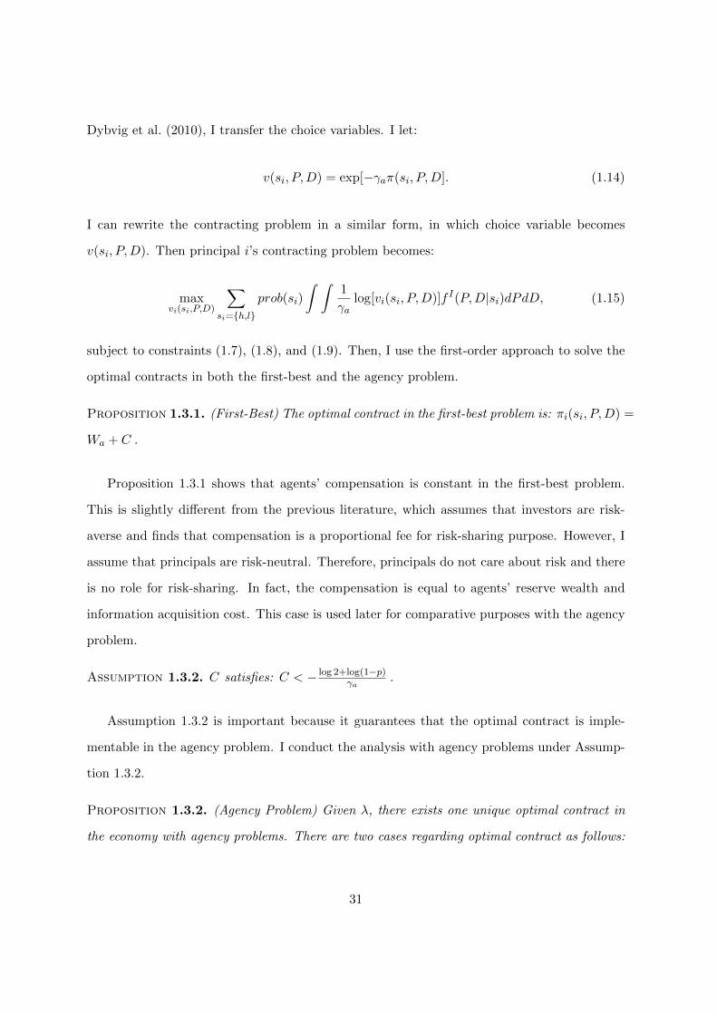
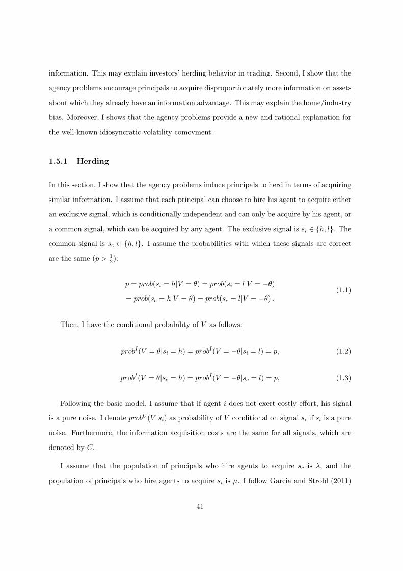
in Figure 4.1.11

This proposition has implications for asset price jumps or excess volatilities. With multiple

equilibria regarding information acquisition, the economy may switch between non-information

equilibrium and high-information equilibria without any relation to fundamentals, leading to

jumps in the asset price and informativeness. Because a jump is an extreme form of excess

volatilities, the same mechanism can also cause excess volatilities in asset price and informa-

tiveness. This result implies that the price informativenesses and institutional ownership are

more volatile for small/growth stocks or during recessions, which are usually associated with

large residual uncertainties. This result also implies that price jumps and excess volatilities

are more likely to occur for small/growth stocks or during recessions, which is consistent with

Bennet, Sias and Starks (2003), Campbell, Lettau, Malkiel and Xu (2001), Xu and Malkiel

(2003), Ang, Hodrick and Zhang (2006, 2009) and Bekaert, Hodrick and Zhang (2012).

I also examine how agency problems affect asset pricing behavior. I focus on the analysis of

price informativeness and return volatility. For price informativeness, because the equilibrium

11I set θ = 2, N = 2, p = 0.6, Wa = 0, C = 0.07. I also set M = 5, M = 20 and M = 200 for low residualuncertainty, median residual uncertainty and high residual uncertainty cases, respectively.

37

Figure 1.4.1: Information Acquisition Benefit

is not a linear function of fundamental value or noisy traders’ demand, the conditional variance

V ar(D|P ) in the conventional literature is not appropriate for my analysis because this measure

depends on the price P . In accordance with Malamud and Petrov (2014), I use the price’s

expected error as price informativeness. When the price is more informative, this expected

error is lower:

E(|V − P ||V ) =θ[N − λ(2p− 1)]

N. (1.1)

For volatility, I calculate the asset return’s volatility V ar(V − P ) as follows:

V ar(V − P ) =M2

3+θ2[N − λ(2p− 1)]

N. (1.2)

When the population of informed principals increases, both the expected error of the price

38

and the volatility decrease. Before proceeding, I know that agency problems negatively affect

the net benefit from information, which decreases the prices informativeness. Then, price

becomes more sensitive to noisy traders’ demand, leading to increased volatility. I denote Bap

as the net benefit of information in an economy with agency problems, and denote Bfb as the

net benefit in the first-best problem. I find the following result:

Lemma 1.4.4. Given λ, the net benefit in the agency problem is lower than the first-best

problem. That is Bap < Bfb.

I then have the formal result regarding price informativeness and volatility.

Proposition 1.4.4. Both price’s expected error and volatility are higher in an economy with

agency problems than the first-best problem.

I examine how different parameters affect the population of informed principals. I focus on

the case in which M is small because a unique equilibrium exists in this case. When the agents’

risk aversion increases, the agency problem becomes more severe and the principals need to

provide higher compensation to agents. Thus, I expect that the equilibrium population of

informed principals decreases with agents’ risk aversion. Furthermore, when M increases, it is

more difficult for principals to monitor agents and the agency problem is exacerbated. Thus, the

equilibrium population of informed principals decreases with residual uncertainty. These results

are shown in the following figures. I note that agents’ risk aversion or residual uncertainty does

not have any impact on the population of informed principals due to the assumption regarding

principals’ risk-neutrality. These two figures show that price informativeness is low during

recessions, which are associated with large uncertainty.12

1.5 Implications

In this section, I extend the basic model in three directions to study its asset pricing implication.

First, I show that the agency problems induce principals to herd in terms of acquiring similar

12I set θ = 2, N = 2, p = 0.6, Wa = 0, γa = 1, C = 0.05 and M = 20 for analysis of agents’ risk aversion. Iset θ = 2, N = 2, p = 0.6, Wa = 0, γa = 1, and C = 0.075 for analysis of residual uncertainty M .

39

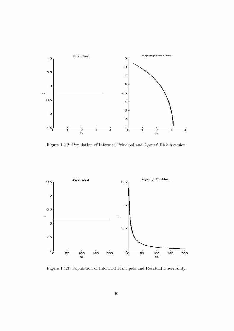
Figure 1.4.2: Population of Informed Principal and Agents’ Risk Aversion

Figure 1.4.3: Population of Informed Principals and Residual Uncertainty

40

information. This may explain investors’ herding behavior in trading. Second, I show that the

agency problems encourage principals to acquire disproportionately more information on assets

about which they already have an information advantage. This may explain the home/industry

bias. Moreover, I shows that the agency problems provide a new and rational explanation for

the well-known idiosyncratic volatility comovment.

1.5.1 Herding

In this section, I show that the agency problems induce principals to herd in terms of acquiring

similar information. I assume that each principal can choose to hire his agent to acquire either

an exclusive signal, which is conditionally independent and can only be acquire by his agent, or

a common signal, which can be acquired by any agent. The exclusive signal is si ∈ {h, l}. The

common signal is sc ∈ {h, l}. I assume the probabilities with which these signals are correct

are the same (p > 12):

p = prob(si = h|V = θ) = prob(si = l|V = −θ)

= prob(sc = h|V = θ) = prob(sc = l|V = −θ) .(1.1)

Then, I have the conditional probability of V as follows:

probI(V = θ|si = h) = probI(V = −θ|si = l) = p, (1.2)

probI(V = θ|sc = h) = probI(V = −θ|sc = l) = p, (1.3)

Following the basic model, I assume that if agent i does not exert costly effort, his signal

is a pure noise. I denote probU (V |si) as probability of V conditional on signal si if si is a pure

noise. Furthermore, the information acquisition costs are the same for all signals, which are

denoted by C.

I assume that the population of principals who hire agents to acquire sc is λ, and the

population of principals who hire agents to acquire si is µ. I follow Garcia and Strobl (2011)

41

to define herding equilibrium as follows:

Definition 1.5.1. Herding Equilibrium: one equilibrium is herding equilibrium if µ = 0 and

λ > 0

This definition is following Hirshleifer and Teoh (2003), who define herding as any behavior

similarity caused by individuals’ interaction. Herding equilibrium occurs only if all informed

principals hire agents to acquire the common signal. As argued by Garcia and Strobl (2011), the

common signal is less valuable for principals than the exclusive signal because of competition.

Thus, without agency problems, herding equilibrium never occur. However, I show that herding

equilibrium may emerge in an economy with agency problems through the following mechanism.

There are two groups of informed principals: the first group acquires sc; the second group

acquires si. Each principal in the first group is indexed by principal i, where i ∈ [0, λ]. And

each principal in the second group is indexed by principal j, where j ∈ [0, µ]. I denote Ecp

and EIp as expected trading profits for principals in the first and second group respectively. I

denote Bcfb and BI

fb as net benefits of information for different groups in the economy without

agency problem. Moreover, I denote Bcap and BI

ap as net benefit of information for different

groups respectively in the economy with agency problems.

For the first group, principal i submits Xi = 1 if sc = h, and submits Xi = −1 if sc = l.

For the second group, principal j submits Xj = 1 if sj = h, and submits Xj = −1 if sj = l.

To simplify the analysis, I only focus on the herding equilibrium. On the herding equilibrium,

µ = 0. In this case, if sc = h, the total orders is X = λ + n. If sc = l, the total orders is

X = −λ + n. Thus, the total orders X is distributed on [−λ −M,λ + M ]. Receiving total

orders, the market maker sets the price as follows:

Lemma 1.5.1. Given λ > 0 and µ = 0, the price follows the rule:

P (X) =

(2p− 1)θ if N − λ < X ≤ N + λ

0 if −N + λ ≤ X ≤ N − λ

−(2p− 1)θ if −N − λ ≤ X < −N + λ

(1.4)

42

To show the existence of a herding equilibrium, I need to calculate expected trading profits

for these two groups. Although there is no second group in the herding equilibrium, I also can

calculate the expected trading profit for this group assuming one principal j is the marginal

principal acquiring an exclusive signal. Then I have the following results:

Lemma 1.5.2. The expected trading profit of principals with the common signal is given by:

Ecp = (2p− 1)θN − λN

. (1.5)

Lemma 1.5.3. The expected trading profit of principals with an exclusive signal is given by:

EIp = (2p− 1)θN − (2p− 1)2λ

N. (1.6)

Lemma 1.5.2 and Lemma 1.5.3 shows that the expected trading profit of principals for the

second group is higher than the first group. There is a large price impact when principals

trade similarly because of having the same information, which makes the total orders more

informative about the common signal and decreases the first group’s information advantage.

Thus, principals have higher incentives to acquire the exclusive signal than the common signal

in the economy without agency problems. However, when the residual uncertainty is sufficiently

large, principals herd to the common signals in the economy with agency problems. Herding

makes the price sensitive to the common signal. Consequently, agents have strong incentives

to acquire the common signal as they can easily forecast the asset price with this signal,

which mitigates agency problems in acquiring it. Although the exclusive signals can generate

more trading profits, agents could not easily forecast asset price with these signals because of

their idiosyncratic noises, which worsens the agency problems in acquiring these signals. This

mechanism generates the herding equilibrium. I show the formal result as follows:

Proposition 1.5.1. Comparing the economy with and without agency problems, I have

(1) no herding equilibrium occurs in the first-best;

92) when M is small enough, no herding equilibrium occurs in the economy with agency prob-

lems; (2) when − log 4p(1−p)γa

< C < (2p−1)θ−Wa and M is large enough, the herding equilibrium

43

exists in the economy with agency problems.

Proposition 1.5.1 shows that the herding equilibrium occurs when the residual uncertainty

is large. This result implies that herding is stronger in small/growth stocks, which have consid-

erable uncertainty. It is consistent with Lakonishok, Shleifer and Vishny (1992) and Wermers

(1999), who find that institutional investors have stronger herding behavior in small/growth

stocks. Although my model is static, it implies that institutional investors tend to follow the

lead of others. When more fund managers trade in one specific stock, others observe this and

tend to follow their lead because these followers anticipate that the price will become more

informative and the agency problems will be mitigated.

1.5.2 Home/Industry Bias

In this section, I explore the model’s implication for the home/industry bias, which is a long-

standing puzzle. As documented by Fama and Poterba (1991), Coval and Moskowitz (1999),

Grinblatt and Keloharju (2001), Huberman (2001) and Seasholes and Zhu (2010), both house-

holds and institutions prefer to trade the assets which are located around their hometowns or

home countries. Though it is possible that some behavior biases drive home bias in house-

holds, home bias among institutional investors is still puzzling because they are sophisticated

investors. Another plausible explanation is that investors have superior information on home

assets, Van Nieuwerburgh and Veldkamp (2009) argue that investors can easily acquire infor-

mation about other assets, which could eliminate home investors’ information advantage and

mitigate home bias. Even if investors can freely acquire information, I show that home bias

still exists with agency problems in information acquisition.

I extend the basic model to consider two groups of principals: the first group has some

opportunity to get free information; the second group has no information. The first group is

interpreted as home principals based on the conventional belief that investors have an infor-

mation advantage on home assets. The population of home principals is denoted by ω. Each

principal in this group is indexed by i, where i ∈ [0, ω]. The second group is called foreign

44

principals. Each principal in this group is indexed by j. Any principals can hire agents to

acquire information. Furthermore, I assume that principal i in the first group is endowed by a

private signal sh,i, which takes the form:

sh,i = {V, ∅}. (1.7)

The feature of this signal is that sh,i is a pure noise when sh,i = ∅, and it is perfectly

informative if sh,i = V . The possibility that sh,i is perfectly informative is denoted by ph:

prob(sh,i = V ) = ph, (1.8)

where 0 < ph < p. There are two differences between home and foreign principals: the first

is that home principals can use their endowed signals in trading; the second difference is that

home principals can use their endowed signals in the contracting.13 Moreover, I assume that

the population of home principals hiring agents is λ, and the population of foreign principals

hiring agents is µ. Although home principals may know the fundamental value exactly, they

also have incentives to acquire information because they have chances to become uninformed.

If the endowed signals are informative, home principals only rely on their endowed signals

in trading. Otherwise, they have to rely on signals from agents. Thus, the total orders is

X = phω + (1 − ph)(2p − 1)λω + (2p − 1)µ + n if V = θ. And the total orders is X =

−phω − (1 − ph)(2p − 1)λω − (2p − 1)µ + n if V = −θ. To simplify the analysis, I let η =

phω + (1− ph)(2p− 1)λω + (2p− 1)µ. Before proceeding, I define two home bias equilibria as

follows:

Definition 1.5.2. Weak Home Bias Equilibrium: one equilibrium is weak home bias equilib-

rium if λ > 0 and µ > 0.

Definition 1.5.3. Strong Home Bias Equilibrium: one equilibrium is strong home bias equi-

13If these signals are not verifiable, there exist some mechanisms inducing principals to reveal their privateinformation, such as imposing an infinite penalty when asset payoff deviates considerably from principals’reports. The infinite penalty can be interpreted as reputation concern. One interpretation of these contracts isthe subjective evaluation. Or this type of contract can be interpreted as an implicit contract.

45

librium if λ > 0 and µ = 0.

Receiving total orders, the market maker sets the price as follows:

P (X) =

θ if N − η < X ≤ N + η

0 if −N + η ≤ X ≤ N − η

−θ if −N − η ≤ X < −N + η

(1.9)

I calculate the expected trading profits for different groups. I denote E1h,p, E

2h,p and Ef,p

as expected trading profits for home principals who hire agents, home principals who do not

hire, and informed foreign principals respectively. They are shown as follows:

Ef,p = (2p− 1)θN − ηN

, (1.10)

E1h,p = [ph + (1− ph)(2p− 1)]θ

N − ηN

, (1.11)

E2h,p = phθ

N − ηN

. (1.12)

It is clear that the gain from information for home principals is (1−ph)(2p−1)θN−ηN , which

is lower than the trading profits of informed foreign principals. This is due to the decreasing

marginal benefits of information. Thus, without agency problems, home principals have lower

incentive than foreign principals to hire agents to acquire information. However, with agency

problems, this is not the case. Home principals can use their endowed information in incentive

provision, agency problems are not severe for home principals and home principals may have

higher incentive to acquire information than foreign principals. The formal results regarding

home bias are as follows:

Proposition 1.5.2. Comparing the economy with and without agency problems, I have

(1) neither weak home bias equilibrium nor strong home bias equilibrium occurs in the first-

best;

(2) when M is small enough, neither weak home bias equilibrium nor strong home bias equi-

46

librium occurs in the economy with agency problem;

(3) when both M and N are large enough, a strong herding equilibrium exists in the economy

with agency problem when θ1 < θ < θ2.

where θ1 and θ2 are defined in the Appendix.

Proposition 1.5.2 shows that home bias occurs when the residual uncertainty is large. This

result implies that home bias is stronger when investors trade small/growth stocks. It is

consistent with Kang and Stulz (1997) and Coval and Moskowitz (1999). For example, Coval

and Moskowitz (1999) find that U.S. fund managers have a stronger home bias when they

trade small stocks. It also implies that investors tend to learn more about the assets within

their expertise. This prediction is consistent with Massa and Simonov (2006), who find that

Swedish investors buy assets highly correlated with their non-financial income.

1.5.3 Idiosyncratic Volatility Comovement

In this section, I explore the model’s implication for idiosyncratic volatility comovement, which

is documented by recent studies (see Bekaert, Hodrick and Zhang, 2012, Kelly, Lustig and

Van Nieuwerburgh, 2013 and Herskovic, Kelly, Lustig and Van Nieuwerburgh, 2013). More

importantly, because recent studies (Bansal, Kiku, Shaliastovich and Yaron, 2014, Campbell,

Giglio, Polk, Turley, 2014 and Herskovic, Kelly, Lustig and Van Nieuwerburgh, 2013) find

that the common factor in idiosyncratic volatilities has significant effects on asset prices, it is

important to understand the driving force. In particular, the common factor in idiosyncratic

volatilities is not related to the conventional risk factors, and the driving force is still puzzling.

I extend the basic model to consider two risky assets. Each asset is indexed by k, where

k = 1, 2. Asset k’s payoff is denoted by Dk, which has a fundamental value Vk and a residual

uncertainty εk. I assume εk is uniformly distributed on [−Mk,Mk], where Mk > 0. Vk takes θk

and −θk with equal probability, where θk > 0. In particular, I assume that two assets’ residual

uncertainties are independent of each other, and also are independent of the two fundamentals.

47

There is a correlation between the two fundamentals as shown:

prob(V2 = θ2|V1 = θ1) = prob(V2 = −θ2|V1 = −θ1) = q, (1.13)

prob(V1 = θ1|V2 = θ2) = prob(V1 = −θ1|V2 = −θ2) = q. (1.14)

The noisy traders’ demand in asset k is denoted by nk following a uniform distribution on

[−Nk, Nk], where Nk > 0. Noisy traders’ demands are independent of other random variables.

I assume that each market has one risk-neutral market maker, who sets the price independently

from each other. The price of asset k is denoted by Pk. Furthermore, there are two groups of

principals: group k can only trade the risky asset k, perhaps due to market segmentation or

trading constraints. The population of informed principals in asset k is λk. To simplify the

analysis, I assume that λ1 is exogenous, and λ2 is endogenous. This assumption is reasonable

in many circumstances. For example, there are some insiders or home investors, who are

endowed with information. The above assumptions are helpful to make the mechanism in my

model clear. If the principals can trade both assets, it is possible that there exist other possible

effects, which may mitigate or exacerbate my mechanism (see Vayanos and Woolley, 2013 and

Cespa and Foucault, 2014). Each informed principal’s signal is denoted by sk,i. Information

structures are the same as the basic model with one risky asset. Then, I have:

probI(Vk = θk|sk,i = h) = probI(Vk = −θk|sk,i = l) = p, (1.15)

To avoid the price of asset 1 being fully informative about the fundamental, I have λ1 <

N12p−1 . Although the principals in group 2 can not trade the risky asset 1, they still can write

contracts on the prices and payoffs of two assets. Specifically, informed principal i in group 2

design contract π2,i(sR(s2,i), P1, P2, D1, D2), where s2,i is his agent’s signal and sR(s2,i) is the

report. The reason why principals in asset 2 write this type of contracts is that two assets’

fundamentals are correlated and agents’ forecasting accuracy for the price of asset 1 is also

related to their effort. I follow the procedure in the basic model to solve the equilibrium prices,

optimal contracts, and population of informed principals in group 2. I carry out the numerical

48

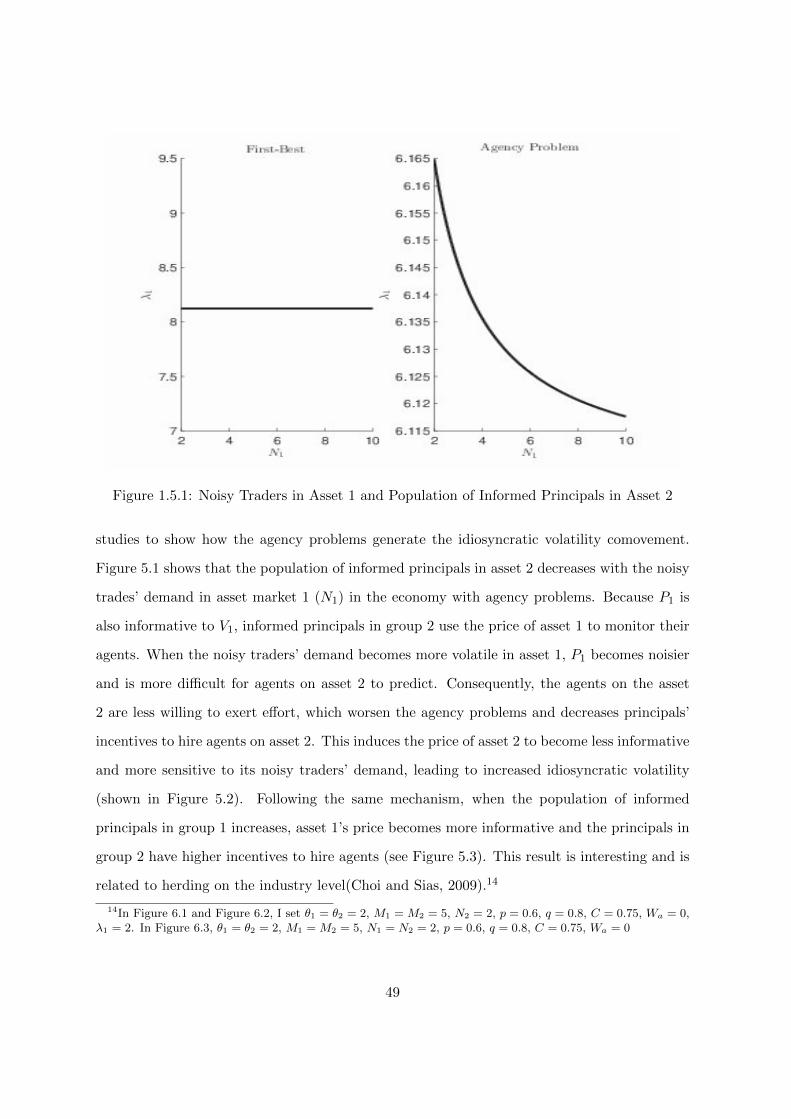
Figure 1.5.1: Noisy Traders in Asset 1 and Population of Informed Principals in Asset 2

studies to show how the agency problems generate the idiosyncratic volatility comovement.

Figure 5.1 shows that the population of informed principals in asset 2 decreases with the noisy

trades’ demand in asset market 1 (N1) in the economy with agency problems. Because P1 is

also informative to V1, informed principals in group 2 use the price of asset 1 to monitor their

agents. When the noisy traders’ demand becomes more volatile in asset 1, P1 becomes noisier

and is more difficult for agents on asset 2 to predict. Consequently, the agents on the asset

2 are less willing to exert effort, which worsen the agency problems and decreases principals’

incentives to hire agents on asset 2. This induces the price of asset 2 to become less informative

and more sensitive to its noisy traders’ demand, leading to increased idiosyncratic volatility

(shown in Figure 5.2). Following the same mechanism, when the population of informed

principals in group 1 increases, asset 1’s price becomes more informative and the principals in

group 2 have higher incentives to hire agents (see Figure 5.3). This result is interesting and is

related to herding on the industry level(Choi and Sias, 2009).14

14In Figure 6.1 and Figure 6.2, I set θ1 = θ2 = 2, M1 = M2 = 5, N2 = 2, p = 0.6, q = 0.8, C = 0.75, Wa = 0,λ1 = 2. In Figure 6.3, θ1 = θ2 = 2, M1 = M2 = 5, N1 = N2 = 2, p = 0.6, q = 0.8, C = 0.75, Wa = 0

49

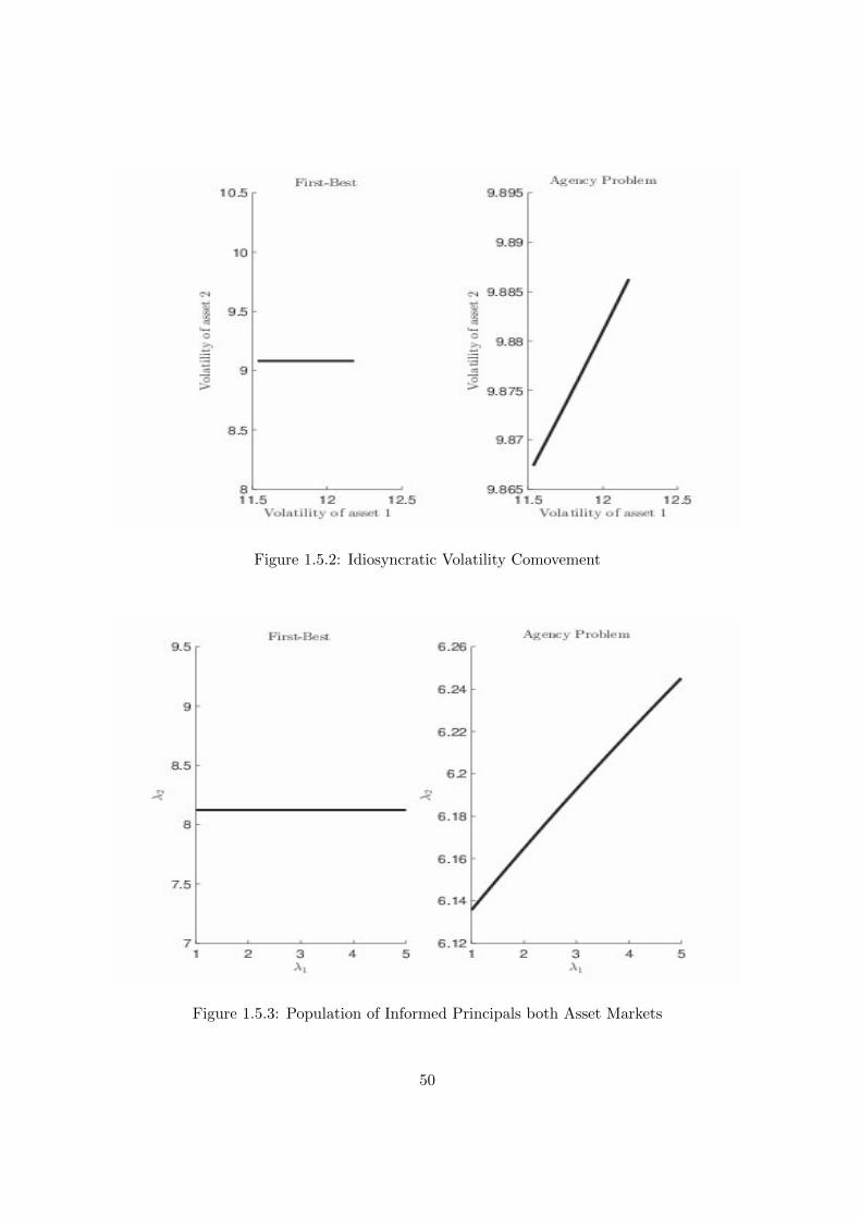
Figure 1.5.2: Idiosyncratic Volatility Comovement

Figure 1.5.3: Population of Informed Principals both Asset Markets

50

1.6 Generalization

My model assumes: (1) agents have CARA utilities; (2) the fundamental value V takes binary

values; (3) principals do not learn information from the asset price. This section relaxes these

assumptions and shows that the strategic complementarities are robust.

1.6.1 General Utility Function of Agents

This section shows that my results are robust when agents have a general hyperbolic absolute

risk aversion (HARA) class of utility functions. The HARA utility function is shown as

follows:

U(W ) =γ

1− γ[AW

γ+K]1−γ , K ≥ 0 (1.1)

where the utility function is only defined over AWγ +K > 0. I know the absolute risk aversion

coefficient is given by:

−U′′

U ′=

Aγ

AW +Kγ(1.2)

When γ < 0, this HARA utility function has an increasing absolute risk aversion, which is

implausible. Thus, I only consider the case where γ > 0. Particularly, this general HARA

utility function has several examples which are largely used in finance or economy, such as

power utility, negative exponential utility or logarithmic utility.

Assumption 1.6.1. γ satisfies: γ > 0.

To simplify the analysis, I assume that agents need to incur a utility loss if they exert effort.

This utility lose is denoted by C. Thus, the participant constraint and incentive constraints

are shown as follows:

∑si={h,l}

prob(si)

∫ ∫{U [πi(si, P,D)]− C}f I(P,D|si)dPdD = U [Wa], (1.3)

where LHS of Equation (1.3) is agent i’s expected utility when he exerts costly effort.

51

Meanwhile, Wa is the reserve wealth of agents.

Ex Ante IC which is the incentive-compatibility of effort constraint

∑si={h,l}

prob(si)∫ ∫{U [πi(si, P,D)]− C}f I(P,D|si)dPdD

≥∑

si={h,l}prob(si)

∫ ∫[U [πi(s

R(si), P,D)]]fU (P,D|si)dPdD(1.4)

Ex Post IC which is incentive-compatibility of truth reporting(∀si and sR(si) : s→ s)

∑si={h,l}

prob(si)∫ ∫{U [πi(si, P,D)]}f I(P,D|si)dPdD

≥∑

si={h,l}prob(si)

∫ ∫[U [πi(s

R(si), P,D)]]f I(P,D|si)dPdD(1.5)

Assumption 1.6.2. I have different cases regarding the information acquisition cost

Case 1: If γ < 1, U(Wa)− C2p−1 > 0;

Case 2: If γ > 1, U(Wa) + C2p−1 < 0;

Case 3: if γ = 1 and K = 0.

This assumption could ensure that the optimal contracts can be implemented and there

is interior solution to the contracting for different γ. I show that strategic complementarity

effect is robust in the following proposition.

Proposition 1.6.1. Under Assumption 1.6.1 and Assumption 1.6.2, when the agents have

HARA utility in the economy with agency problems, I have the following results:

(1)for small enough M , information acquisition delegation is a strategic substitute. That is ,

∂B∂λ < 0.

(2) for large enough M , there exists λgc satisfying: when λ < λgc, information acquisition

delegation is a strategic complement. That is ∂B∂λ > 0.

52

1.6.2 More General Distribution of V

In this section, I assume that V takes three values in θ, 0 or −θ. In particular, the distribution

of V is symmetric. The probability that V = 0 is denoted as pm. The probability of V = θ or

V = −θ is given by:

prob(V = θ) = prob(V = −θ) = (1− pm)/2, (1.6)

After exerting effort, agent i generates a private signal si ∈ {h, 0, l} about the risky asset’s

fundamental value V . The probability with which a signal is correct by

prob(si = h|V = θ) = prob(si = 0|V = 0) = prob(si = l|V = −θ) = p, (1.7)

and

prob(si = 0|V = θ) = prob(si = 0|V = −θ) = (1− p)q, (1.8)

and

prob(si = l|V = θ) = prob(si = h|V = −θ) = (1− p)(1− q), (1.9)

and

prob(si = h|V = 0) = prob(si = l|V = −θ) = (1− p)/2, (1.10)

where si is independent across agents and p ≥ 13 , while q ≥ 1

2 . Principal i submits Xi = 1 when

he receives report si = h, does nothing when he receives report si = 0, and submits Xi = −1

53

when he receives report si = l. Then the market maker sets the price as follows:

P (X) =

θ if N < X ≤ N + λ(p− (1− p)(1− q))

θ 1−pm1+pmif N − λ(p− (1− p)(1− q)) < X ≤ N

0 if −N + λ(p− (1− p)(1− q)) ≤ X

≤ N − λ(p− (1− p)(1− q))

−θ 1−pm1+pmif −N ≤ X < −N + λ(p− (1− p)(1− q))

−θ if −N − λ(p− (1− p)(1− q)) ≤ X < −N

(1.11)

It is clear that the price increases with the total orders X. It differs from the binary-state

case on the feature that the price takes five values. This difference also shows that the problem

will become extremely complicate when I consider more a general distribution of V . I carry

out the numerical studies to show that information acquisition complementarities is robust

in Figure 6.1, as is the relation between residual uncertainty/agents’ risk aversion and price

informativeness in Figure 6.2 and Figure 6.3.15

1.6.3 Learning

This section shows that my results are robust when principals learn information from the asset

price. To obtain analytical solution in the non-linear REE, I modify the information structure

and the distribution of residual uncertainty. I assume that the residual uncertainty ε follows

normal distribution N(0, σ2M ). The private signal acquired by agent i is denoted by si. Through

the costly effort ei ∈ {0, e}, the joint distributions of his signal si and the fundamental value

V is a mixture distribution as follows:

(b+ ei)fI(si, V ) + (1− b− ei)fU (si, V ), (1.12)

15I set θ = 2, N = 2, p = 0.6, pm = 0.5, q = 0.6, Wa = 0, C = 0.07. I also set M = 5, M = 20 and M = 200for low residual uncertainty, median residual uncertainty and high residual uncertainty cases respectively inFigure 6.1. Then set θ = 2, N = 2, p = 0.6, pm = 0.5, q = 0.6, Wa = 0, gammaa = 1, C = 0.05 and M = 20for analysis of agents’ risk aversion in Figure 6.2. I set θ = 2, N = 2, p = 0.6, pm = 0.5, q = 0.6, Wa = 0,gammaa = 1, and C = 0.075 for analysis of residual uncertainty M in Figure 6.3.

54

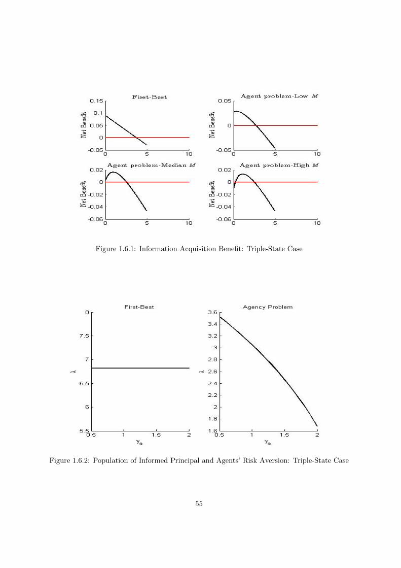
Figure 1.6.1: Information Acquisition Benefit: Triple-State Case

Figure 1.6.2: Population of Informed Principal and Agents’ Risk Aversion: Triple-State Case

55

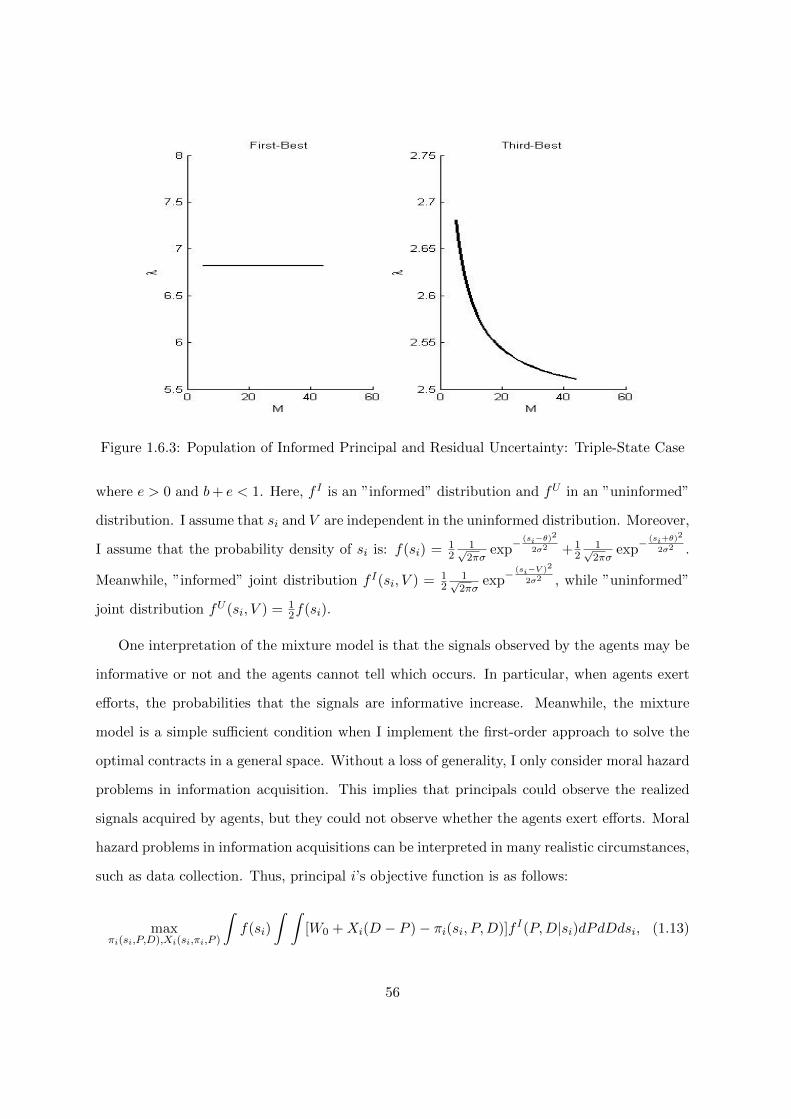
Figure 1.6.3: Population of Informed Principal and Residual Uncertainty: Triple-State Case

where e > 0 and b+ e < 1. Here, f I is an ”informed” distribution and fU in an ”uninformed”

distribution. I assume that si and V are independent in the uninformed distribution. Moreover,

I assume that the probability density of si is: f(si) = 12

1√2πσ

exp−(si−θ)

2

2σ2 +12

1√2πσ

exp−(si+θ)

2

2σ2 .

Meanwhile, ”informed” joint distribution f I(si, V ) = 12

1√2πσ

exp−(si−V )2

2σ2 , while ”uninformed”

joint distribution fU (si, V ) = 12f(si).

One interpretation of the mixture model is that the signals observed by the agents may be

informative or not and the agents cannot tell which occurs. In particular, when agents exert

efforts, the probabilities that the signals are informative increase. Meanwhile, the mixture

model is a simple sufficient condition when I implement the first-order approach to solve the

optimal contracts in a general space. Without a loss of generality, I only consider moral hazard

problems in information acquisition. This implies that principals could observe the realized

signals acquired by agents, but they could not observe whether the agents exert efforts. Moral

hazard problems in information acquisitions can be interpreted in many realistic circumstances,

such as data collection. Thus, principal i’s objective function is as follows:

maxπi(si,P,D),Xi(si,πi,P )

∫f(si)

∫ ∫[W0 +Xi(D − P )− πi(si, P,D)]f I(P,D|si)dPdDdsi, (1.13)

56

where Xi(si, πi, P ) is principal i’s demand function conditional on the price P and the signal

si reported by his agent. He maximizes his utility function subject to his agent’s participant

constraint and incentive compatibility as follows:

PC:

∫f(si)

∫ ∫[− exp−γaπi(si,P,D)+γaC ]f I(P,D|si)dPdDdsi = − exp(−γaWa), (1.14)

IC: ∫f(si)

∫ ∫[− exp−γaπi(si,P,D)+γaC ]f I(P,D|si)dPdDdsi

≥∫f(si)

∫ ∫[− exp−γaπi(si,P,D)+γaC ]fU (P,D|si)dPdDdsi,

(1.15)

where f I(P,D|si) is the conditional probability density given that the agent i exerts effort,

and fU (P,D|si) is the conditional probability density given that the agent i shirks.

Now, I assume that there is one continuum of principals and the population of principals hir-

ing agents to acquire information is λ. For the informed principal i, the probability density of si

conditional on V = θ is denoted by ηI,i,h, where ηI,i,h = 1+b+e2

1√2πσ

exp−(s−θ)2

2σ2 +1−e−b2

1√2πσ

exp−(s+θ)2

2σ2 ;

the probability density of si conditional on V = −θ is denoted by ηI,i,l, where ηI,i,l =

1+b+e2

1√2πσ

exp−(s+θ)2

2σ2 +1−e−b2

1√2πσ

exp−(s−θ)2

2σ2 . For the uninformed principal i,the probability

density of si conditional on V = θ is denoted byηU,i,h, where ηU,i,h = 1+b2

1√2πσ

exp−(s−θ)2

2σ2 +1−b2

1√2πσ

exp−(s+θ)2

2σ2 ;

the probability density of si conditional on V = −θ is denoted byηU,i,l, where ηU,i,l = 1+b2

1√2πσ

exp−(s+θ)2

2σ2 +1−b2

1√2πσ

exp−(s−θ)2

2σ2 .

Due to the assumption about risk-neutral principals, the optimal contracts and asset pricing

can be solved separately as our basic model. I solve the model following step-by-step: (1) in

the first step, I solve the asset pricing; (2) in the second step, I solve the optimal contract

given the population of informed principals; (3)in the third step, I calculate the net benefit of

information acquisition to show the strategic complementaries.

Asset Pricing In order to maximize the final wealth, it is necessary to compute the

conditional expectation of V for different groups. According to the Bayes’s rule, the posterior

probability pK(si, P ) of state h for principal i of type K after observing si and P is given by:

57

pK(si, P ) =fh(P )ηK,i,h

fh(P )ηK,i,h + fl(P )ηK,i,l(1.16)

where fω(P ), ω = h, l is the probability density of the equilibrium price conditional on

the corresponding state of the world. Given the posterior probabilities, principals’ demand

schedules are shown in the following lemma.

Lemma 1.6.1. For any K = I, U , there exists a threshold XK(P ) such that the demand

schedule for principal i of type K is given by:

XK,i =

1 if si ≥ XK(P ) ,

−1 if si < XK(P ) ,

(1.17)

where the threshold XK(P ) is uniquely determined by the condition:

pK(XK(P ), P ) =P + θ

2θ. (1.18)

Having showing the demand schedules, the aggregate demand can be calculated as follows.

Conditional on V = θ, the aggregate demand is given by

D(P, θ) = λ[1− (1 + b+ e)Φ(XI(P )− θ)− (1− b− e)Φ(XI(P ) + θ)] (1.19)

+(1− λ)[1− (1 + b)Φ(XU (P )− θ)− (1− b)Φ(XU (P ) + θ)]; (1.20)

conditional on V = −θ, the aggregate demand is given by

D(P,−θ) = λ[1− (1 + b+ e)Φ(XI(P ) + θ)− (1− b− e)Φ(XI(P )− θ)] (1.21)

+(1− λ)[1− (1 + b)Φ(XU (P ) + θ)− (1− b)Φ(XU (P )− θ)], (1.22)

where Φ is the cumulative distribution function for normal distribution N(0, σ2). Consequently,

given realized demand from noisy traders, the market clearing condition takes the form as

58

follows:

D(P, V ) = n (1.23)

Thus, the probability density of price P conditional on the value V is denoted as fi(P ). They

are calculated as follows:

fh(P ) = λ2N [(1 + b+ e)φ(XI(P )− θ) + (1− b− e)φ(XI(P ) + θ)]X

′I(P )

+ (1−λ)2N [(1 + b)φ(XU (P )− θ) + (1− b)φ(XU (P ) + θ)]X

′U (P )

(1.24)

fl(P ) = λ2N [(1 + b+ e)φ(XI(P ) + θ) + (1− b− e)φ(XI(P )− θ)]X ′I(P )

+ (1−λ)2N [(1 + b)φ(XU (P ) + θ) + (1− b)φ(XU (P )− θ)]X ′U (P )

(1.25)

where φ is the probability density function for the normal distribution N(0, σ2). The key to

solve the asset pricing is to solve the thresholds XI and XU . I follow Malamud and Petrov

(2014) to solve both. I denote the likelihood ratio by:

LK(X) = ηK,i,h/ηK,i,l. (1.26)

From the Lemma 1.6.1, I have the following condition:

LI(XI(P )) = LU (XU (P )). (1.27)

Thus, the relation between XU (P ) and XI(P ) is: XU (P ) = L−1U (LI(XI(P ))). It indicates that

the solution of XI can characterize the asset pricing. I have the following result regarding XI ,

XU and the probability density of price P :

Proposition 1.6.2. There exists a monotone increasing, absoluately continuous solution

XI(P ), P ∈ (−θ, θ) to

2 logLK(XI(P )) = logP + θ

θ − P.

59

Meanwhile, XI(P ), XU (P ) = L−1U (LK(XI(P ))) and

fh(P ) = λ2N [(1 + b+ e)φ(XI(P )− θ) + (1− b− e)φ(XI(P ) + θ)]X

′I(P )

+ (1−λ)2N [(1 + b)φ(XU (P )− θ) + (1− b)φ(XU (P ) + θ)]X

′U (P )

, (1.28)

and

fl(P ) = λ2N [(1 + b+ e)φ(XI(P ) + θ) + (1− b− e)φ(XI(P )− θ)]X ′I(P )

+ (1−λ)2N [(1 + b)φ(XU (P ) + θ) + (1− b)φ(XU (P )− θ)]X ′U (P )

(1.29)

form a rational expectations equilibrium.

Contracting I use the first-order approach to solve the optimal contracts. First, I let l1

and l2 be the Lagrange multipliers on the PC and IC. I can get the expression for optimal

compensation as follows:

π(si, P,D) =log(l1 + l2 − l2 exp

−γaC fU (P,D|si)fI(P,D|si)

) + log(γa)

γa(1.30)

Net Benefit of Information Now I calculate the net benefit of information. Conditional

on the fundamental value V and asset price P , the expected trading profit of principal i of

type K = I, U is calculated by:

EK,h,P = prob(si < XK(P )|V = θ, P )(P − θ) + prob(si ≥ XK(P )|V = θ, P )(θ − P )

= 1+b+e2 Φ(XK − θ)(P − θ) + 1−b−e

2 Φ(XK + θ)(P − θ)

+1+b+e2 [1− Φ(XK − θ)](θ − P ) + 1−b−e

2 [1− Φ(XK + θ)](θ − P ),

(1.31)

EK,l,P = prob(si < XK(P )|V = −θ, P )(P + θ) + prob(si ≥ XK(P )|V = −θ, P )(−θ − P )

= 1+b+e2 Φ(XK + θ)(P + θ) + 1−b−e

2 Φ(XK − θ)(P + θ)

+1+b+e2 [1− Φ(XK + θ)](−θ − P ) + 1−b−e

2 [1− Φ(XK − θ)](−θ − P ).

(1.32)

60

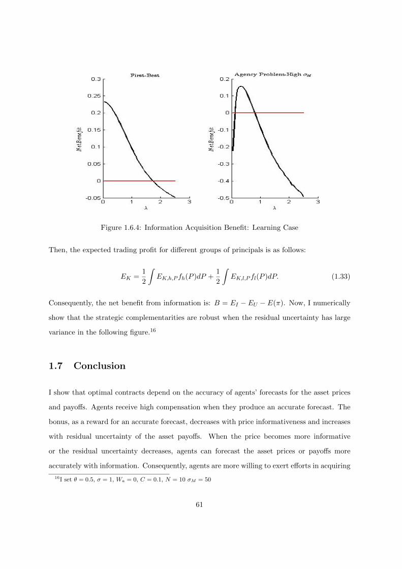
Figure 1.6.4: Information Acquisition Benefit: Learning Case

Then, the expected trading profit for different groups of principals is as follows:

EK =1

2

∫EK,h,P fh(P )dP +

1

2

∫EK,l,P fl(P )dP. (1.33)

Consequently, the net benefit from information is: B = EI − EU − E(π). Now, I numerically

show that the strategic complementarities are robust when the residual uncertainty has large

variance in the following figure.16

1.7 Conclusion

I show that optimal contracts depend on the accuracy of agents’ forecasts for the asset prices

and payoffs. Agents receive high compensation when they produce an accurate forecast. The

bonus, as a reward for an accurate forecast, decreases with price informativeness and increases

with residual uncertainty of the asset payoffs. When the price becomes more informative

or the residual uncertainty decreases, agents can forecast the asset prices or payoffs more

accurately with information. Consequently, agents are more willing to exert efforts in acquiring

16I set θ = 0.5, σ = 1, Wa = 0, C = 0.1, N = 10 σM = 50

61

information. Thus, the principals can decrease the bonus. These results predict that the

bonus is larger for professionals, who trade or cover small/growth stocks with larger residual

uncertainty or assets with lower institutional ownership.

More importantly, I show that agency problems in delegated information acquisition play

important roles in shaping institutional investors’ behavior and asset pricing. The novelty

of my model is that agency problems generate a strategic complementarities in information

acquisition delegation. When more principals hire agents to acquire information, the price

becomes less noisy, which make it easier for agents to forecast. Therefore, agents are more

willing to exert effort, thereby mitigating agency problems. In turn, other principals are more

willing to hire agents. These strategic complementarities lead to multiple equilibria, which

have implications for jumps and excess volatilities in asset prices or price informativeness. In

particular, multiple equilibria occur when the asset payoff’s residual uncertainty is large. This

can provide a potential explanation for observed excess volatilities in small/growth stocks or

during recessions. My results also predict that price informativeness or institutional ownership

tend to have jumps for small/growth stocks. The extensions of this model demonstrate that

the agency problems could provide explanations for some phenomena, including idiosyncratic

volatility comovement, herding behavior and home/industry bias. Moreover, my model predicts

that the herding or home/industry bias is stronger for small/growth stocks.

The driving force for my results is as follows: the price becomes more informative when more

principals hire agents to acquire information, which mitigates agency problems. Thus, it is

clear that the assumptions about risk-averse principals will not overturn the main mechanisms.

However, relaxing these assumptions is interesting. If principals are risk-averse, I expect that

the optimal contract will consist of two components: the first is agents’ forecasting accuracy,

and the second is proportional fee attributable to risk sharing. I leave this extension for further

study.

62

Bibliography

Admati, Anat, and Paul Pfleiderer, (1986). “A Monopolistic Market of Information.” Journal of

Economic Theory, July: 400-438.

Admati, Anat, and Paul Pfleiderer, (1988). “Selling and Trading on Information in Financial

Markets.” American Economic Review, May: 96-103.

Admati, Anat, and Paul Pfleiderer, (1990). “Direct and Indirect Sale of Information.” Econo-

metrica, 58: 901-928.

Admati, Anat, and Paul Pfleiderer, (1997). “Does it All Add Up? Benchmarks and the Compen-

sation of Active Portfolio Managers.” Journal of Business, July: 323-350.

Agarwal, Vikas, Naveen Daniel, and Narayan Y. Naik (2009). “Role of Managerial Incentives

and Discretion in Hedge Fund Performance.” Journal of Finance, 44: 2221-2256.

Asparouhova, Elena, Peter Bossaerts, Jernej Copic, Bradford Cornell, Jaksa Cvitanic,

and Debrah Meloso (2010). “Experiments on Asset Pricing Under Delegated Portfolio Manage-

ment.” Working paper.

Acharya, Viral V., Marco Pagano, and Paolo Volpin (2013). “Seeking Alpha: Excess Risk

Taking and Competition for Managerial Talent.” Working paper.

Albagli, Elias, Christian Hellwig, and Aleh Tsyvinski (2013). “A Theory of Asset Pricing

Based on Heterogeneous Information.” Working paper.

Allen, Franklin (1990). “The Market for Information and the Origin of Financial Intermediation.”

Journal of Financial Intermediation, 1: 3-30.

Allen, Franklin (2001). “Do Financial Institutions Matter.” Journal of Finance, 56: 1165-75.

63

Ang, Andrew, Robert Hodrick, and Xiaoyan Zhang (2006). “The Cross-Section of Volatility

and Expected Returns.” Journal of Finance, 61: 259-299.

Ang, Andrew, Robert Hodrick, and Xiaoyan Zhang (2009). “High Idiosyncratic Volatility and

Low Returns: International and Further U.S. Evidence.” Journal of Financial Economics, 97: 279-

301.

Bansal, Ravi, Dana Kiku, Ivan Shaliastovich and Amir Yaron (2014). “Volatility, the Macroe-

conomy, and Asset Prices.” The Journal of Finance.

Basak, Suleyman, and Dmitry Makarov (2014). “Strategic Asset Allocation in Money Manage-

ment.” Journal of Finance, 69, 1, 179-217.

Basak, Suleyman and Anna Pavlova. “Asset Prices and Institutional Investors.” American Eco-

nomic Review, 103(5): 1728-58.

Basak, Suleyman, Anna Pavlova and Alexander Shapiro (2007). “Optimal Asset Allocation

and Risk Shifting in Money Management.” Review of Financial Studies, 20: 1583-1621.

Basak, Suleyman, Anna Pavlova and Alexander Shapiro (2008). “Offsetting the Implicit In-

centives: Benefits of Benchmarking in Money Management.” Journal of Banking and Finance, 32:

1882-1993.

Basak, Suleyman, Alexander Shapiro and Lucie Tepla (2006). “Risk Management with Bench-

marking.” Management Science, 52: 542-557.

Barlevi, Gadi, and Pietro Veronesi (2000). “Information Acquisition in Financial Markets.” The

Review of Economics Studies, 67: 79-90.

Bekaert, Geert, Robert Hodrick and Xiaoyan Zhang (2012). “Aggregate Idiosyncratic Volatil-

ity.” Journal of Financial and Quantitative Analysis, 47: 1155-1185.

Bennet, James A., Richard W.Sias and Laura T. Starks (2003). “Greener Pastures and the

Impact of Dynamic Institutional Preferences.” Review of Financial Studies, 16(4): 1203-1238.

Berk, Jonathan B., and Jules H. van Binsbergen (2013). “Measuring Managerial Skill in the

Mutual Fund Industry.” Working paper.

Berk, Jonathan B., and Richard C. Green (2004). “Mutual Fund Flows and Performance in

Rational Markets.” Journal of Political Economy, 112, 1269-1295.

64

Bhattacharya, Sudipto, and Paul Pfleiderer (1985). “Delegated portfolio management.” Journal

of Economic Theory, 36, 163-87.

Biais, Bruno, and Laurent Germain (2002). “Incentive-Compatible Contracts for the Sale of

Information.” Review of Financial Studies, 15(4), 987-1003.

Breon-Darish, Bradyn M. (2013). “On Existence and Uniqueness of Equilibrium in a Class of Noisy

Rational Expectations Models.” Working paper.

Buffa, Andrea M., Dimitr Vayanos and Paul Woolley (2013). “Asset Management Contracts

and Equilibrium Prices.” Working paper.

Campbell, John, Martin Lettau, Burton G. Malkiel and Yexiao Xu (2001). “Have Individual

Stocks Become More Volatile? An Empirical Exploration of Idiosyncratic Risk.” Journal of Finance,

56(1), 1-43.

Campbell, John, Stefano Giglio, Christopher Polk and Robert Turley (2014). “An In-

tertemporal CAPM with Stochastic Volatility.” Working paper.

Carpenter, Jennifer N (2000). “Does Option Compensation Increase Managerial Risk Appetite?”

Journal of Finance, 55, 2311-2331.

Cespa, Giovanni and Thierry Foucault (2014). “Illiquidity Contagion and Liqidity Crashes.”

Review of Financial Studies, forthcoming.

Chevalier, Judith and Glenn Ellison (1999). “Career Concerns of Mutual Fund Managers.”

Quarterly Journal of Economics, 114, 389-432.

Choi, Nicole and Richard W. Sias (2009). “Institutional Industry Herding .” Journal of Financial

Economics, 94(3), 469-491.

Cohen, Randy, Christopher Polk and Bernhard Silli (2010). “Best Ideas.” Working paper.

Coval, Joshua D. and Tobias Moskowitz (1999). “Home Bias at Home: Local Equity Preference

in Domestic Portfolios.” The Journal of Finance, 54(6), pp. 2045-73.

Das, Sanjiv Ranjan and Rangarajan K. Sundaram (2002). “Fee Speech: Signaling, RiskSharing,

and the Impact of Fee Structures on Investor Welfare.” Review of Financial Studies, 15(5), 1465-1497.

65

Dasgupta, Amil and Andrea Prat (2006). “Financial Equilibrium with Career Concerns.” Theo-

retical Economics, 1(1), 67-93.

Dasgupta, Amil and Andrea Prat (2008). “Information Aggregation in Financial Markets with

Career Concerns.” Journal of Economic Theory, 143, 83-113.

Dasgupta, Amil, Andrea Prat and Michela Verardo (2011). “The Price Impact of Institutional

Herding.” The Review of Financial Studies, 24, 892-925.

DeLong, J. Bradford, Andrei Shleifer, Lawrence H. Summers and RobertWaldmann

(1990). “Positive Feedback Investment Strategies and Destabilizing Rational Speculation.” Jour-

nal of Finance, 45, 379-395.

Dow, James and Garry Gorton (1997). “Noise Trading, Delegated Portfolio Management, and

Economic Welfare.” Journal of Political Economy, 105: 1024-50.

Dow, James, Itay Goldstein and Alexander Guembel (2011). “Incentives for Information

Production in Markets where Prices Affect Real Investment.” Working paper.

Dybvig, Philip H, Heber Farnsworth and Jennifer N. Carpenter (2010). “Portfolio Perfor-

mance and Agency.” Review of Financial Studies, 23, 1-23.

Fama, Eugene F., and James M. Poterba (1991). “Investor Diversification and International Equity

Markets.” American Economic Review, 81: 222-226.

French, Kenneth R, (2008). “Presidential address: The cost of active investing” Journal of Finance,

63: 1537-1573.

Froot, Kenneth, David Scharfstein and Jeremy Stein(1992). “Herd on the Street: Informa-

tional Inefficiencies in a Market with Short-Term Speculation.” Journal of Finance, 47: 1461-1484.

Garcia, Diego and Gunter Strobl (2011). “Relative Wealth Concerns and Complementarities in

Information Acquisition.” Review of Financial Studies, 24(1), 169-207.

Garcia, Diego and Joel Vanden (2009). “Information acquisition and mutual funds.” Journal of

Economic Theory, 144(5), 1965-1995.

Grleanu, Nicolae and Lasse Heje Pedersen (2011). “Margin-based Asset Pricing and Deviations

from the Law of One Price.” Review of Financial Studies, 24(6), 1980-2022.

66

Goldstein, Itay, Yan Li and Liyan Yang (2013). “Speculation and Hedging in Segmented Markets.”

forthcoming in Review of Financial Studies.

Goldstein, Itay, Emre Ozdenoren and Kathy Yuan (2013). “Trading Frenzies and Their Impact

on Real Investment.” Journal of Financial Economics, 109(2), 566-582.

Goldstein, Itay, Emre Ozdenoren and Kathy Yuan (2011). “Learning and Complementarities

in Speculative Attacks.” Review of Economic Studies, 78(1), 263-292.

Gompers, Paul A. and Andrew Metrick (2001). “Institutional Investors and Equity Prices.”

Quarterly Journal of Economics, 116: 229-59.

Grossman, Sanford J. and Oliver Hart (1983). “Distance, Language, and Culture Bias: The Role

of Investor Sophistication.” Journal of Finance, 56: 1053-1073.

Grossman, Sanford J. and Oliver Hart (1983). “An Analysis of the Principal-Agent Problem.”

Econometrica, 51: 7-45.

Grossman, Sanford J. and Joseph E. Stiglitz (1980). “On the Impossibility of Informationally

Efficient Markets.” American Economic Review, 116: 229-59.

Grundy, Bruce D., and Maureen McNichols (1980). “Trade and the Revelation of Information

through Prices and Direct Disclosure.” Review of Financial Studies, 2(4): 495-526.

Guerrieri, Veronica and Peter Kondor (2012). “Fund Managers, Career Concerns, and Asset

Price Volatility.” American Economic Review, 102, 5 : 1986-2017.

Hayek, Friedrich (1945). “The Use of Knowledge in Society.” American Economic Review, 35:

519-530.

He, Zhiguo and Arvind Krishnamurthy (2012). “A Model of Capital and Crises.” Review of

Economic Studies, 79(2) : 735-777.

He, Zhiguo and Arvind Krishnamurthy (2013). “Intermediary Asset Pricing.” American Economic

Review, 103(2) : 732-770.

Hellwig, Martin F (1980). “On the Aggregation of Information in Competitive Markets.” Journal

of Economic Theory, 22, 3 : 477-498.

67

Hellwig, Christian and Laura Veldkamp (2009). “Knowing What Others Know: Coordination

Motives in Information Acquisition.” Review of Economic Studies, 76 : 223-251.

Hellwig, Christian, Arijit Mukherji and Laura Veldkamp (2006). “Self-Fulfilling Currency

Crises: The Role of Interest Rates.” American Economic Review, 95, 5 : 1769-1787.

Herskovic, Bernard, Bryan T. Kelly, Hanno N. Lustig and Stijn Van Nieuwerburgh (2013).

“The Common Factor in Idiosyncratic Volatility: Quantitative Asset Pricing Implications.” Working

paper.

Hirshleifer, David and Siew Hong Teoh (2003). “Herd Behaviour and Cascading in Capital

Markets: a Review and Synthesis.” European Finance Management, 9, 1 : 25-36.

Holmstrom, Bengt (1979). “Moral Hazard and Observability.” Bell Journal of Economics, 10, 74-91.

Holmstrom, Bengt (1982). “Moral Hazard in Teams.” Bell Journal of Economics, 13, 324-340.

Huang, Shiyang, Dong Lou and Christopher Polk (2014). “The Booms and Busts of Beta

Arbitrage.” Working paper.

Huberman, Gur (2001). “Familiarity Breeds Investment.” Review of Financial Studies, 14, 659-680.

Huberman, Gur and Shmuel Kandel (1993). “On the Incentives for Money Managers: A Signaling

Approach.” European Economic Review, 37, 5 : 1065-1081.

Jones, Charles M. and Marc L. Lipson (2004). “Are Retail Orders Different?” Working paper,

Columbia University.

Kacperczyk, Marcin, Clemens Sialm and Lu Zheng (2005). “On the Industry Concentration of

Actively Managed Equity Mutual Funds.” The Journal of Finance, 60, 1983-2012.

Kacperczyk, Marcin, Clemens Sialm and Lu Zheng (2007). “Industry Concentration and Mutual

Fund Performance.” The Journal of Finance, 62, 485-528.

Kacperczyk, Marcin, Stijn Van Nieuwerburgh and Laura Veldkamp (2013a). “Time-Varying

Fund Manager Skill.” The Journal of Finance, 69, 4 : 1455-1484.

Kacperczyk, Marcin, Stijn Van Nieuwerburgh and Laura Veldkamp (2013b). “Rational

Attention Allocation over the Business Cycle.” Working paper.

68

Kaniel, Ron and Pter Kondor (2013). “The Delegated Lucas Tree.” Review of Financial Studies,

26, 4: 929-984.

Kaniel, Ron and Pter Kondor (2013). “Why is there a home bias? an analysis of foreign equity

ownership in Japan,.” Journal of Financial Economics, 46(1), 3-28.

Keynes, John Maynard, (1936). “The General Theory of Employment, Interest, and Money..”

London: Macmillan.

Kelly, Bryan T., Hanno N. Lustig and Stijn Van Nieuwerburgh (2013). “Firm Volatility in

Granular Networks.” Working paper.

Kyle, Albert S (1985). “Continuous Auctions and Insider Trading.” Econometrica, 53: 1315-35.

Kyle, Albert S, Hui Ou-Yang and Bin Wei (2011). “A Model of Portfolio Delegation and Strategic

Trading.” Review of Financial Studies, 24: 3778-812.

Lakonishok, Josef, Andrei Shleifer and Robert W. Vishny (1992). “The Impact of Institutional

Trading on Stock Prices.” The Journal of Finance, 41: 951974.

Li, C. Wei and Ashish Tiwari (2009). “Incentive Contracts in Delegated Portfolio Management.”

Review of Financial Studies, 22, 4, 681-714.

Dong Lou and Christopher Polk (2014). “Comomentum: Inferring Arbitrage Activity from Return

Correlations.” Working paper.

Malamud, Semyon and Evgeny Petrov (2014). “Portfolio Delegation and Market Efficiency.”

Working paper.

Makarov, Igor and Guillaume Plantin (2012). “Rewarding Trading Skills Without Inducing

Gambling.” forthcoming in The Journal of Finance.

Massa, Massimo and Andrei Simonov (2006). “Hedging, Familiarity and Portfolio Choice.” Review

of Financial Studies, 19(2), 633-685.

Ou-Yang, Hui (2003). “Optimal Contracts in a Continuous-Time Delegated Portfolio Management

Problem.” Review of Financial Studies, 16: 173-208.

Ozdenoren, Emre and Kathy Yuan (2008). “Feedback Effects and Asset Prices.” The Journal of

Finance, 63(4), 1939-1975.

69

Ozdenoren, Emre and Kathy Yuan (2014). “Endogenous Contractual Externalities.” Working

paper.

Panageas, Stavros and Mark M. Westerfield (2009). “Optimal Contracts in a Continuous-Time

Delegated Portfolio Management Problem.” Review of Financial Studies, 16: 173-208.

Pastor, Lubos and Robert F. Stambaugh (2012). “On the Size of the Active Management Indus-

try.” Journal of Political Economy, 120: 740-781.

Seasholes, Mark S. and Ning Zhu (2010). “Individual Investors and Local Bias.” The Journal of

Finance, 65, 5, 1987-2010.

Shleifer, Andrei and Robert W. Vishny (1997). “The Limits of Arbitrage.” The Journal of

Finance, 52, 1, 35-55.

Tyler Shumway, Maciej Szefler and Kathy Yuan (2011). “The Information Content of Revealed

Beliefs in Portfolio Holdings.” Working paper.

Sias, Richard W. (2004). “Institutional Herding.” Review of Financial Studies, 17(1): 165-206.

Starks, Laura T (1987). “Performance Incentive Fees: An Agency Theoretical Approach.” Journal

of Financial and Quantitative Analysis, 22: 17-32.

Stein, Jeremy (1987). “Informational Externalities and Welfare-Reducing Speculation,.” Journal of

Political Economy, 95: 1123-1145.

Stein, Jeremy (2009). “Sophisticated Investors and Market Efficiency.” The Journal of Finance, 4:

1517-1548.

Stoughton, Neal M (1993). “Moral Hazard and the Portfolio Management Problem.” The Journal

of Finance, 48: 2009-28.

Van Nieuwerburgh, Stijin and Laura Veldkamp (2009). “Information Immobility and the Home

Bias Puzzle.” The Journal of Finance, 64: 1187-1215.

Van Nieuwerburgh, Stijin and Laura Veldkamp (2009). “Information Acquisition and Under-

Diversification.” Review of Economic Studies, 77: 779-805.

Vayanos, Dimitri and Paul Woolley (2013). “An Institutional Theory of Momentum and Reversal.”

Review of Finance Studies, 26 (5): 1087-1145.

70

Veldkamp, Laura (2006a). “Information Markets and the Comovement of Asset Prices.” Review of

Economic Studies, 73: 823-845.

Veldkamp, Laura (2006b). “Media Frenzies in Markets for Financial Information.” American Eco-

nomic Review, 96, 3: 577-601.

Wermers, Russ (1999). “Mutual Fund Herding and the Impact on Stock Prices.” The Journal of

Finance, 54, 2: 581-622.

Xu, Yexiao and Burton G. Malkiel (2003). “Investigating the Behavior of Idiosyncratic Volatility.”

Journal of Business, 76: 613-644.

71

1.8 Appendix

1.8.1 Proofs

This appendix provides all proofs omitted above.

Proof of Lemma 1.3.1. If λ ≥ N2p−1 , market maker will know that V = θ if X > −N +

λ(2p− 1) and V = −θ if X < N − λ(2p− 1). Then market makers will always set P = V . If

this is the case, informed investors’ trading will always equals to zero because Xi(V −P ) = 0.

If the trading profit is zero, investors have no incentive to acquire information. Thus I can

conclude that the population of informed investors can not be larger than N2p−1 .

Proof of Lemma 1.3.2. On the support [−λ(2p−1)−N,λ(2p−1)+N ], the conditional pdf

of X follows

f(X|V = θ) =

1 if −N + λ(2p− 1) ≤ X ≤ N + λ(2p− 1)

0 if X < −N + λ(2p− 1)

(1.1)

f(X|V = −θ) =

0 if X > N − λ(2p− 1)

1 if −N − λ(2p− 1) ≤ X ≤ N − λ(2p− 1)

(1.2)

Using Bayesian updating, prob(V = θ|X) =12f(X|V=θ)

12f(X|V=θ)+ 1

2f(X|V=−θ) . Thus conditional on X,

market maker’s belief about probability of V = θ follows:

prob(V = θ|X) =

1 if N − λ(2p− 1) < X ≤ N + λ(2p− 1)

12 if −N + λ(2p− 1) ≤ X ≤ N − λ(2p− 1)

1 if −N − λ(2p− 1) ≤ X ≤ −N + λ(2p− 1)

(1.3)

Then because P = prob(V = θ|X)θ − [1− prob(V = θ|X)]θ, I can get the price function.

72

Proof of Lemma 1.3.3 and Lemma 1.3.4. Step 1 f I(P = θ,D, si = h) = f I(P = θ,D|si =

h)× prob(si = h).Then

f I(P = θ,D, si = h) = prob(P = θ, si = h)× f I(D|P = θ, si = h)

= prob(V = θ, si = h)× prob(N − λ(2p− 1) ≤ n ≤ N + λ(2p− 1))× f I(D|P = θ, si = h)

=

1

2Mp2λ(2p−1)

N if −M + θ ≤ D ≤M + θ

0 if −M − θ ≤ D < −M + θ

(1.4)

Since prob(si = h) = 12 , I can get t f I(P = θ,D|si = h) in the Lemma.

Step 2 f I(P = −θ,D, si = h) = f I(P = −θ,D|si = h)× prob(si = h). Then

f I(P = −θ,D, si = h) = prob(P = −θ, si = h)× f I(D|P = −θ, si = h)

= prob(V = −θ, si = h)× prob(N − λ(2p− 1) ≤ n ≤ −N + λ(2p− 1))× f I(D|P = −θ, si = h)

=

0 if M − θ < D ≤M + θ

12M

1−p2

λ(2p−1)N if −M − θ ≤ D ≤M − θ

(1.5)

Since prob(si = h) = 12 , I can get f I(P = −θ,D|si = h) in the Lemma.

73

Step 3 f I(P = 0, D, si = h) = f I(P = 0, D|si = h)× prob(si = h). Then

f I(P = 0, D, si = h) = prob(P = 0, si = h)× f I(D|P = 0, si = h)

= prob(V = θ, si = h)× prob(−N + λ(2p− 1) ≤ n ≤ N − λ(2p− 1))× f I(D|P = θ, si = h)

+prob(V = −θ, si = h)× prob(−N + λ(2p− 1) ≤ n ≤ N − λ(2p− 1))× f I(D|P = −θ, si = h)

=

p4M

N−λ(2p−1)N if M − θ ≤ D ≤M + θ

14M

N−λ(2p−1)N if −M + θ ≤ D < M − θ

1−p4M

N−λ(2p−1)N if −M − θ ≤ D < −M + θ

(1.6)

Step 4: Then Lemma 1.3.3 and Lemma 1.3.4 can be derived following the same process

above.

Proof of Proposition 1.3.1. I prove this proposition in two steps.

Step 1 (proof of existence and uniquess)

maxvi(si,P,D)

∑si={h,l}

∑P={−θ,0,θ}

1

2

∫ ∫1

γalog[vi(si, P,D)]f I(P,D|si)dD, (1.7)

subject to participation constraint:

∑si={h,l}

∑P={−θ,0,θ}

1

2vi(si, P,D)f I(P,D|si)dD = exp−γaWa−γaC (1.8)

Then I let f =∑

si={h,l}∑

P={−θ,0,θ}12

∫ ∫log[vi(si, P,D)]f I(P,D|si)dD and then

D1= {−∑

si={h,l}

∑P={−θ,0,θ}

1

2vi(si, P,D)f I(P,D|si)dD ≥ − exp−γaWa−γaC} (1.9)

It is obvious that f is a strictly concave function and D1 is convex. Then I can conclude

that the local maximum of f over D1 is a global solution to this optimization. This implies

that the solution in the first-order approach is the global solution to this problem.

74

Step 2: (Solution). I denote Lagrange multiplier of by λ1. Then I can get vi(si, P,D) =

1γa

1λ1

and 1γaλ1

= exp−γaWa−γaC . Then I can conclude that πi(si, P,D) = Wa + C.

Proof of Proposition 1.3.2. Step 1 (proof of existence and uniquess in the second-best)

The second-best case is proposed by Dybvig et al. (2010) where the principals are able to

observe agents’ signals, but are not able to observe agents’ hidden actions. Thus, there is not

misreporting problem. Then I will show that the agency problem in my study is equivalent to

this second-best case since the signals or fundamental value V take binary states. Particularly,

the IC in the second-best case is:

∑si={h,l}

1

2

∫ ∫vi(si, P,D)[f I(P,D|si)− exp−γaC fU (P,D|si)]dPdD ≤ 0 (1.10)

Then I let f =∑

si={h,l}∑

P={−θ,0,θ}12

∫ ∫log[vi(si, P,D)]f I(P,D|si)dD and then

D2= {−∑

si={h,l}∑

P={−θ,0,θ}12vi(si, P,D)f I(P,D|si)dD ≥ − exp−γaWa−γaC ;∑

si={h,l}

12

∫ ∫vi(si, P,D)[f I(P,D|si)− exp−γaC fU (P,D|si)]dPdD ≤ 0}

vi(si, P,D) ≥ 0

(1.11)

It is obvious that f is a strictly concave function over D2, while D2 is convex. Then I can

conclude that the local maximum of f over D2 is a global solution to this optimization. This

implies that the solution in the first-order approach is the global solution to this problem.

Step 2 (case when p = 1). The first order condition should be:

1 = [λ1 + λ2 − λ2exp−γaC f(P,D)

f I(P,D|si)]γavi(si, P,D) (1.12)

When p = 1, if λ2 > 0 I have following cases:

when si = h and P = −θ: λ1 + λ2 − λ2exp−γaC f(P,D)

f I(P,D|si)= −∞ (1.13)

75

when si = h , P = 0 and −M−θ ≤ D < −M+θ: λ1+λ2−λ2exp−γaC f(P,D)

f I(P,D|si)= −∞ (1.14)

when si = l and P = θ: λ1 + λ2 − λ2exp−γaC f(P,D)

f I(P,D|si)= −∞ (1.15)

when si = l , P = 0 and M − θ ≤ D ≤M + θ: λ1 + λ2 − λ2exp−γaC f(P,D)

f I(P,D|si)= −∞ (1.16)

First-order approach will fail here and this indicates that λ2 = 0. When λ2 = 0, I can

conclude that IC will not be binding. I substitute 1 = λ1γavi(si, P,D) into PC and get 1λ1γa

= exp−γaWa−γaC . Then I can get result shown in the proposition.

Step 3: (case when p < 1). I denote Lagrange multiplier of PC by λ′1 and Lagrange

multiplier of IC by λ′2 . Then I can get

1 = [λ′1 + λ

′2 − λ

′2

exp−γaC f(P,D)

f I(P,D|si)]γavi(si, P,D) (1.17)

Then I let: λ1 = λ′1γa, λ2 = λ

′2γa and q = exp−γaC (where q < 1)

From Lemma 1.3.3 and Lemma 1.3.4, I know that:

(1) When si = h,

1

vi(si = h, P = θ,D)= λ1 + λ2 − λ2

q

2p(1.18)

1

vi(si = h, P = −θ,D)= λ1 + λ2 − λ2

q

2(1− p)(1.19)

76

1

vi(si = h, P = 0, D)=

λ1 + λ2 − λ2 q

2p if M − θ ≤ D ≤M + θ

λ1 + λ2 − λ2q if −M + θ ≤ D < M − θ

λ1 + λ2 − λ2 q2(1−p) if −M − θ ≤ D < −M + θ

(1.20)

(2) When si = l,

1

vi(si = l, P = θ,D)= λ1 + λ2 − λ2

q

2(1− p)(1.21)

1

vi(si = l, P = −θ,D)= λ1 + λ2 − λ2

q

2p(1.22)

1

vi(si = l, P = 0, D)=

λ1 + λ2 − λ2 q

2(1−p) if M − θ ≤ D ≤M + θ

λ1 + λ2 − λ2q if −M + θ ≤ D < M − θ

λ1 + λ2 − λ2 q2p if −M − θ ≤ D < −M + θ

(1.23)

To simplify the analysis, I let x = λ1 + λ2 − λ2 q2p and y = λ1 + λ2 − λ2 q

2(1−p) . Then it is

clear that I have λ1 + λ2 − λ2q = px+ (1− p)y. I substitute vi(si = l, P = 0, D) into PC and

IC.

Step 4 (case when p < 1). After rearrangment, I have:

1xp

λ(2p−1)N + 1

xpθM

N−λ(2p−1)N + 1

px+(1−p)yM−θM

N−λ(2p−1)N

+ 1y(1−p)θM

N−λ(2p−1)N + 1

y (1− p)λ(2p−1)N = exp−γaWa−γaC(1.24)

1

y=

1

x+

exp−γaWa(1− exp−γaC)

(p− 12)(λ(2p−1)N + θ

MN−λ(2p−1)

N )(1.25)

77

I let a1 = λ(2p−1)N + θ

MN−λ(2p−1)

N , a2 = exp−γaWa (1−exp−γaC)p−0.5 , then I have y = a1x

a1+a2x. From the

above two equations, I have:

a1x

+1− a1

px+ (1− p) a1xa1+a2x

= exp−γaWa −exp−γaWa(1− exp−γaC)

2p− 1(1.26)

I let g(x) = a1x + 1−a1

px+(1−p) a1xa1+a2x

. It is obvious that g(x) is a decreasing function of x when

x > 0. This concludes that there exists unique solution. Let b = exp−γaWa − exp−γaWa (1−exp−γaC)2p−1 .

It is obvious that there is one unique positive solution when b > 0. I have:

x =−[ba1+(1−p)a1a2−a2]+

√[ba1+(1−p)a1a2−a2]2+4bpa2a12bpa2

and y = a1xa1+a2x

Step 5: Now I prove that this second-best is equivalent to the agency problem in my model.

I need to prove that agents’ utility in truth telling is higher than that when they misreport after

receiving informative signals, while agents’ utility in truth telling in information acquisition is

higher than that when they randomly reports without any information. This is to prove that :

1xp

λ(2p−1)N + 1

xpθM

N−λ(2p−1)N + 1

px+(1−p)yM−θM

N−λ(2p−1)N

+ 1y(1−p)θM

N−λ(2p−1)N + 1

y (1− p)λ(2p−1)N

≤ 1yp

λ(2p−1)N + 1

ypθM

N−λ(2p−1)N + 1

px+(1−p)yM−θM

N−λ(2p−1)N

+ 1x(1−p)θM

N−λ(2p−1)N + 1

x(1− p)λ(2p−1)N

(1.27)

Since 1y >

1x and p > 1

2 , it is easy to show the above inequality always holds.

Proof of Corollary 1.3.1 and Proof of Proposition 1.3.3 . First, because y = a1xa1+a2x

,

it is obvious that Sf = 1γa

log(1+ exp−γaWa (1−exp−γaC)p−0.5

xλ(2p−1)

N+ θM

N−λ(2p−1)N

). I let z = xλ(2p−1)

N+ θM

N−λ(2p−1)N

.

For Sf , the signs of∂Sf∂λ and

∂Sf∂M depend on ∂z

∂λ and ∂z∂M respectively. For the equation

a1x + 1−a1

px+(1−p) a1xa1+a2x

= b, the LHS is decreasing with z and decrease with a1. Because RHS is

78

constant with a1, then I know that ∂z∂a1

< 0. Then I have

∂z

∂λ=

∂z

∂a1(1− θ

M)(2p− 1)

N< 0 (1.28)

∂z

∂M= − ∂z

∂a1

θ

M2

N − λ(2p− 1)

N> 0 (1.29)

From equation, it is clear that when θ = M , I have ∂z∂λ = 0.

Proof of Lemma 1.4.1 and Proposition 1.4.1. When si = h, I know that Xi = 1; When

si = l, Xi = −1. So I can calculate expected trading profit as follows:

Ep = prob(si = h)E(D − P |si = h) + prob(si = l)E(P − P |si = l) (1.30)

= θ(2p− 1)N − λ(2p− 1)

N(1.31)

Then it is obvious that ∂B∂λ < 0.

Proof of Proposition 1.4.2. Let K = 12a1 log(x)+ 1

2a1 log(y)+(1−a1) log[px+(1−p)y], I can

get B = θ(2p−1)N−λ(2p−1)N −K. Then∂B∂λ = − θ(2p−1)2N − ∂K

∂a1∂a1∂λ = − θ(2p−1)2

N − ∂K∂a1

(1− θM ) θ(2p−1)N .

Step 1 (M is small enough) I know that for M > θ, limM→θ∂B∂λ = − θ(2p−1)2

N < 0. Because

∂B∂λ is a continuous function, this implies that there exists a cutoff M c satisfying M < M c,

∂B∂λ < 0.

Step 2 (M is large enough) I know that forM = +∞, limλ→0∂B∂λ = − θ(2p−1)2

N −lima1→0∂K∂a1

θ(2p−1)N

lima1→0∂K∂a1

= lima1→0{12 log(x) + 12 log(y)− log[px+ (1− p)y]

+12a1

1x∂x∂a1

+ 12a1

1y∂y∂a1

+ (1− a1) 1px+(1−p)y [p ∂x∂a1 + (1− p) ∂y∂a1 ]}

(1.32)

Because y = a1xa1+a2x

, I know that lima1→0 x = 1bp , lima1→0 y = 0, lima1→0

∂x∂a1

= finite

79

lima1→0∂y∂a1

= lima1→0(x

a1+a2x− a1x

(a1+a2x)2+ a1

a1+a2x∂x∂a1− a1x

(a1+a2x)2∂x∂a1

) = finite.

Thus I can obtain lima1→0∂K∂a1

= −∞. Then I can conclude that when M is large enough

and λ small enough, ∂B∂λ > 0. This concludes my proof.

Proof of Proposition 1.4.3. Step 1. When λ = 0, I know that Bap(0) = θ(2p− 1) + log b.

Step 2. If Bap(0) < 0 and maxλ<λfb B(λ) < 0, the unique equilibrium is no information

acquisition equilibrium.

Step 3. If Bap(0) < 0 and maxλ<λfb Bap(λ) > 0, I prove that there exist three equilibria.

The first one is non-information acquisition equilibrium becasue Bap(0) < 0 and∂Bap(0)∂λ > 0.

I let λ∗ be the solution to maxλ<λfb B(λ). Then there exists one solution in (0, λ∗). Moreover,

because Bap < Bfb, I know that B(λfb) < 0, thus exists one solution in (λ∗, λfb). Step 4. If

Bap(0) > 0, because Bap(λfb) < 0, then there exists at least one positive solution in (0, λfb)

Proof of Proposition 1.4.4. This result is direct because I know that Bap < Bfb.

Proof of Lemma 1.5.1. I know that E(V |X) = θp(V = θ|X) − θp(V = −θ|X). Then

because p(V = θ|X) = p(V=θ,X)P (X) ,then I have:

p(V = θ,X) =

p2 if N − λ < X ≤ N + λ

12 if −N + λ ≤ X ≤ N − λ

1−p2 if −N − λ ≤ X < −N + λ

(1.33)

p(V = −θ,X) =

1−p2 if N − λ < X ≤ N + λ

12 if −N + λ ≤ X ≤ N − λ

p2 if −N − λ ≤ X < −N + λ

(1.34)

80

Then I have:

p(V = θ|X) =

p if N − λ < X ≤ N + λ

12 if −N + λ ≤ X ≤ N − λ

1− p if −N − λ ≤ X < −N + λ

(1.35)

Thus, I conclude the proof.

Proof of Lemma 1.5.2. The proof is shown as follows:

Ecp = p(sc = h)E(V − P |sc = h) + p(sc = l)E(P − V |sc = l)

= (2p− 1)θN−λN

(1.36)

Proof of Lemma 1.5.3. Because

E(P |sj = h) = (2p− 1)θ ∗ prob(sc = h|sj = h) λN

−(2p− 1)θ ∗ prob(sc = l|sj = h) λN

= θ λN (2p− 1)3

(1.37)

Following the same logic, I can get E(P |sj = l) = −θ λN (2p−1)3. Then I calculate expected

trading profit of investors who acquire private signal as:

EIp = (2p− 1)θN−(2p−1)2λ

N(1.38)

Proof of Proposition 1.5.1. Step 1. I prove that no herding equilibrium occurs in the econ-

omy without agency problem. Following the analaysis of optimal contract, I know that the

81

payments π = Wa + C. Then when λ > 0 and µ = 0 in the herding equilibriu, I will have

Ecp−Wa−C = 0 > EIp−Wa−C. Because this is impossible, I conclude that herding equilibrium

will not occur.

Step 2. I calculate the optimal payment scheme provided by principals who acquire sc in the

herding equilibrium. Because f I(P = −(2p−1)θ,D|sc = h) = f I(P = (2p−1)θ,D|sc = l) = 0,

the optimal scheme following the proof of Proposition 2.2, I know that

π(P = −(2p− 1)θ, sc = h,D) = π(P = (2p− 1)θ, sc = l,D) = −∞ (1.39)

Otherweise, π = Wa + C.

Step 3. I calculate the optimal payment scheme provided by principals who acquire si in

the herding equilibrium in this step. Before calculation of optimal payment scheme, I calculate

pdf of P and D conditional on si. To simply the analysis, I only consider the case when M

goes to infinity. When M goes to infinity, I know that pdf of P and D conditional on si is

equivalent to pdf of P conditional on si. Then I have the following cases if agents acquire

information:

probI(P |si = h) =

λ[p2+(1−p)2]N if P = (2p− 1)θ

N−λN if P = 0

2λp(1−p)N if P = −(2p− 1)θ

(1.40)

probI(P |si = l) =

2λp(1−p)N if P = (2p− 1)θ

N−λN if P = 0

λ[p2+(1−p)2]N if P = −(2p− 1)θ

(1.41)

Then I have the following cases if agents do not acquire information:

82

probU (P ) =

λ2N if P = (2p− 1)θ

N−λN if P = 0

λ2N if P = −(2p− 1)θ

(1.42)

Following the first-order approach in above proof, I know that

1

v(si = h, P = (2p− 1)θ)=

1

v(si = l, P = −(2p− 1)θ)= λ1 + λ2 − λ2

exp(−γaC)

2[p2 + (1− p)2](1.43)

1

v(si = h, P = −(2p− 1)θ)=

1

v(si = l, P = (2p− 1)θ)= λ1 + λ2 − λ2

exp(−γaC)

4p(1− p)(1.44)

1

v(si = h, P = 0)=

1

v(si = l, P = 0)= λ1 + λ2 − λ2 exp(−γaC) (1.45)

I let p1 = p2 + (1− p)2, x1 = λ1 + λ2 − λ2 exp(−γaC)2p1

, y1 = λ1 + λ2 − λ2 exp(−γaC)2(1−p1) , a11 = λ

N ,

a21 = exp(−γaWa)(1−exp−γaC)p1−0.5 and b1 = exp−γaWa − exp(−γaWa)(1−exp−γaC)

2p1−1 . When b1 < 0, the

solution to solve the optimal contract does not exists.

Step 4. If exp−γaWa − exp(−γaWa)(1−exp−γaC)2p1−1 < 0 and Ecp = (2p− 1)θN−λN −Wa − C > 0 for

some positive λ, I can get the results in the proposition.

Proof of Proposition 1.5.2. Step 1. In the first-best case, it is clear that the optimal pay-

ment scheme is constant. That is π = Wa+C. Because the net befit of information acquisition

for home investors is (1 − ph)(2p − 1)θN−ηN − Wa − C and the net benefit of information

acquisition for foreign investors is (2p− 1)θN−ηN −Wa − C. If λ > 0, this indicates that

83

(1− ph)(2p− 1)θN − ηN

−Wa − C = 0 (1.46)

Moreover, this indicates that (2p−1)θN−ηN −Wa−C > 0. Thus, it implies that µ should be

infinity. This is impossible because price will be fully revealing when µ goes to infinity. Then

trading profit will become zero and this violate the assumption that (1 − ph)(2p − 1)θN−ηN −

Wa − C = 0. Therefore, I can conclude that λ = 0. This implies that neither weak herding

equilibrium not strong herding equilibrium occur in the first-best case.

Step 2. I only prove that strong herding equilibrium occurs under some condition in the

economy with agency problem. Particularly, I try to find the condition under which λ = 1

and µ = 0. For the foreign investors, the approach to solve the optimal contract is simila to

the proof of Proposition 3.2. I only replace λ(2p − 1) with η in the proof. When both of M

and N go to infinity, I know that net benefit of information acquisition for foreign investors is

Bf,ap(0) = (2p− 1)θ + log[exp−γaWa − exp−γaWa (1−exp−γaC)2p−1 ].

Step 3. I take the following steps to solve the optimal contract for the home investors. The

conditional pdf of sh,i when si is informative is shown as follows:

probI(sh,i|si = h) =

php if sh,i = θ

1− ph if sh,i = ∅

ph(1− p) if sh,i = −θ

(1.47)

probI(sh,i|si = l) =

ph(1− p) if sh,i = θ

1− ph if sh,i = ∅

php if sh,i = −θ

(1.48)

84

The conditional pdf of sh,i when si is uninformative is shown as follows:

probU (sh,i) =

ph2 if sh,i = θ

12 if sh,i = ∅

ph2 if sh,i = −θ

(1.49)

Following the first-order approach in proof of Proposition, I know that

1

v(si = h, sh,i = θ)=

1

v(si = l, sh,i = −θ)= λ1 + λ2 − λ2

exp(−γaC)

2p(1.50)

1

v(si = h, sh,i = −θ)=

1

v(si = l, sh,i = θ)= λ1 + λ2 − λ2

exp(−γaC)

2(1− p)(1.51)

1

v(si = h, sh,i = ∅)=

1

v(si = l, sh,i = ∅)= λ1 + λ2 − λ2 exp(−γaC) (1.52)

This is similar to the proof of Proposition 3.2, I let x = λ1+λ2−λ2 exp(−γaC)2p , y = λ1+λ2−

λ2exp(−γaC)2(1−p) , a12 = ph, a22 = exp(−γaWa)(1−exp−γaC)

p−0.5 and b2 = exp−γaWa − exp(−γaWa)(1−exp−γaC)2p−1 .

Following proof of Proposition 4.2, I know that the net benefit of informaiton acquisition

for home investors is Bh,ap(ph) = (1− ph)(2p− 1)θ−K (where K = 12ph log(x) + 1

2ph log(y) +

(1− ph) log[px+ (1− p)y] ).

When ph = 0, I know that Bh,ap(0) = (2p − 1)θ + log[exp−γaWa − exp−γaWa (1−exp−γaC)2p−1 ].

Then I denote the derivative of Bh,ap(ph) with ph by∂Bh,ap∂ph

. Then I know that for very

small positive ε, I know that Bh,ap(ε) = (2p − 1)θ + log[exp−γaWa − exp−γaWa (1−exp−γaC)2p−1 ] +

ε ∗ ∂Bh,ap∂ph. Because

∂Bh,ap(0)∂ph

is infinity and θ is not in the function Bh,ap, there exists small

enough θ satisfying (2p − 1)θ + log[exp−γaWa − exp−γaWa (1−exp−γaC)2p−1 ] = −ε. In this case, I

know that Bh,ap(ε) > 0 and Bh,ap(0) < 0. I let θ1 =− log[exp−γaWa − exp−γaWa (1−exp−γaC )

2p−1]−ε

2p−1 and

θ2 =− log[exp−γaWa − exp−γaWa (1−exp−γaC )

2p−1]

2p−1 . This implies foreign investors never have incentive

to acquire information, but home investors have incentive to acquire informtion under the

85

condition:θ1 < θ < θ2.

Proof of Proposition 1.6.1. Following the similar process in the proof of Proposition 1.3.2

and Proposition 1.4.2, I know that

πi(si = h, P = θ,D) = πi(si = l, P = −θ,D) = π1 (1.53)

πi(si = h, P = −θ,D) = πi(si = l, P = θ,D) = π3 (1.54)

πi(si = h, P = 0, D) =

π1 if M − θ ≤ D ≤M + θ

π2 if −M + θ ≤ D < M − θ

π3 if −M − θ ≤ D < −M + θ

(1.55)

πi(si = l, P = 0, D) =

π3 if M − θ ≤ D ≤M + θ

π2 if −M + θ ≤ D < M − θ

π1 if −M − θ ≤ D < −M + θ

(1.56)

As I know thatπ1 > π2 > π3 if all PC and IC in the second-best are binding as shown

below. Then it is similar as proof of Proposition 1.3.2, I know that this contract can satisfies

ex ante IC and ex post IC. Then I let U1 = U(π1),U2 = U(π2) and U3 = U(π3). Particularly,

the PC and IC follows:

a1pU1 + (1− a1)U2 + a1(1− p)U3 = U(Wa) + C (1.57)

86

U1 = U3 +C

a1(p− 0.5)(1.58)

It is clear that U2 = U(Wa)− C2p−1 −

a11−a1U3.

Now I prove information acquisition complementarity is robust when M is infinite and λ

is small enough for different γ as follows.

Now the principals’ optimization problem becomes to minimize

minπ1,π2,π3

a1pπ1 + (1− a1)π2 + a1(1− p)π3 (1.59)

This problem can be transferred to:

minU3

G(U3) (1.60)

where G(U3) = a1pU−1(U3 + C

a1(p−0.5)) + (1 − a1)U−1(U(Wa) − C2p−1 −

a11−a1U3) + a1(1 −

p)U−1(U3).

Since a1 is a linear function of λ. The first-order condition with λ is equivalent to the

first-order condition with a1, I have ∂G(U3)∂U3

= 0. It is easy to check that Assumption ass:crra

can ensure there exists interior solution to the contracting problem. Particularly, I have the

following three cases:

Case 1: If 0 < γ < 1, I know that I U3 should satisfy: U3 > 0 and U(Wa)− C2p−1−

a11−a1U3 >

0.

Case 2: If γ > 1, I know that U3 should satisfy: U3+ Ca1(p−0.5) < 0,U3 < 0 and

U(Wa)− C2p−1

1−a1 −a1

1−a1U3 < 0.

Case 3: If γ = 1 and K = 0, then I know that U(W ) u ln(W ) (where u represents liner

transformation).

87

It is obvious that U−(x) = [(1−γγ x)1

1−γ −K] γA . I let the solution to this problem to be U∗3 .

Then the minimum value of G(U3) is G(a1, U∗3 ). Now I have effect of a1 on G(a1, U

∗3 ) is:

∂G(a1,U∗3 )∂a1

= pU−1(U3 + Ca1(p−0.5))− U

−1(U(Wa)− C2p−1 −

a11−a1U3) + (1− p)U−1(U3)

+∂G(a1,U∗3 )

∂U∗3

∂G(U∗3 )∂a1

− a1p∂[U−1(U3+

Ca1(p−0.5)

)]

∂(U3+C

a1(p−0.5))

Ca21(p−0.5)

+(1− a1)∂[U−1(

U(Wa)− C2p−1

1−a1− a1

1−a1U3)]

∂(U(Wa)− C

2p−11−a1

− a11−a1

U3)

(− 1(1−a1)2U3)

(1.61)

For any cases, I know that∂G(a1,U∗3 )

∂U∗3

∂G(U∗3 )∂a1

= 0. I show information acquisition is complemen-

tary case by case.

Case 1( γ < 1): I know that: (1 − a1)∂[U−1(

U(Wa)− C2p−1

1−a1− a1

1−a1U3)]

∂(U(Wa)− C

2p−11−a1

− a11−a1

U3)

(− 1(1−a1)2U3) < 0 because

U3 < 0

and −U−1(U(Wa)− C2p−1 −

a11−a1U3) + (1− p)U−1(U3) < 0

and then pU−1(U3+C

a1(p−0.5))−p∂[U−1(U3+

Ca1(p−0.5)

)]

∂(U3+C

a1(p−0.5))

Ca1(p−0.5) = p γA(1−γγ )

11−γ (U3+

Ca1(p−0.5))

11−γ−1[U3−

γ1−γ

Ca1(p−0.5) ]− p

γAK < p γA(1−γγ )

11−γ ( C

a1(p−0.5))1

1−γ−1[U3 − γ1−γ

Ca1(p−0.5) ]− p

γAK

Because U3 > 0 and U3 < U(Wa) + C, I know that lima1→0∂G(a1,U∗3 )

∂a1= −∞. For the net

benefit of information acquisition B, I have lima1→0∂B∂a1

= ∞ for large enough M and small

enough λ.

Case 2 ( γ > 1) From the proof of , I know that p(Aπ1γ + K)γ+ (1 − p)(Aπ3γ + K)γ =

(Aπ2γ +K)γ .

Let π′i = (Aπ1γ + K)γ , I know that πi = [(π

′i)

1γ −K] γA , which is a concave function of π

′i.

Then I can have

pU−1(U3+ Ca1(p−0.5))−U

−1(U(Wa)− C2p−1−

a11−a1U3)+(1−p)U−1(U3) = p π1+(1−p)π3−π2 <

0

Becasue U−(x) = [(1−γγ x)1

1−γ−K] γA , I know that ∂[U−1(x)]∂x = 1

A(1−γγ x)1

1−γ−1 and ∂2[U−1(x)]∂x2

>

0

88

Then from FOC ∂G(U3)∂a1

= 0, I know that

a1p∂[U−1(U3 + C

a1(p−0.5))]

∂(U3 + Ca1(p−0.5))

+(1−a1)∂[U−1(U(Wa)− C

2p−1 −a1

1−a1U3)]

∂(U(Wa)− C2p−1 −

a11−a1U3)

+a1(1−p)∂[U−1(U3)]

∂(U3)= 0

(1.62)

Thus, I have

p∂[U−1(U3+

Ca1(p−0.5)

)]

∂(U3+C

a1(p−0.5))

Ca1(p−0.5)+

∂[U−1(U(Wa)− C

2p−11−a1

− a11−a1

U3)]

∂(U(Wa)− C

2p−11−a1

− a11−a1

U3)

11−a1U3 = p

∂[U−1(U3+C

a1(p−0.5))]

∂(U3+C

a1(p−0.5))

[ Ca1(p−0.5)−

a1U3(1−a1)2 ]− a1U3

(1−a1)2 (1− p)∂[U−1(U3)]∂(U3)

Because [U(Wa)− C2p−1 ]1−a1a1

< U3 < − Ca1(p−0.5) , I know that lima1→0

Ca1(p−0.5) −

a1U3(1−a1)2 =

∞.

For ∂[U−1(x)]∂x = 1

A(1−γγ x)1

1−γ−1, I know that lima1→0∂[U−1(U3)]∂(U3)

= 0 because U3 → −∞.

Because U3 + Ca1(p−0.5) > U(Wa) + C, I have

∂[U−1(U3+C

a1(p−0.5))]

∂(U3+C

a1(p−0.5))

> ∂[U−1(x)]∂x |x=U(Wa)+C

Thus, I can conclude that

lima1→0 p∂[U−1(U3+

Ca1(p−0.5)

)]

∂(U3+C

a1(p−0.5))

Ca1(p−0.5) +

∂[U−1(U(Wa)− C

2p−11−a1

− a11−a1

U3)]

∂(U(Wa)− C

2p−11−a1

− a11−a1

U3)

11−a1U3 =∞

Therefore, it is easy to show that lima1→0∂G(a1,U∗3 )

∂a1= −∞ and I conclude that lima1→0

∂B∂a1

=

∞ for large enough M and small enough λ.

Case 3 forU(W ) = ln(W ), I directly calculate

∂G(U3)∂a1

= a1p exp(U3 + Ca1(p−0.5)) + a1(1− p) exp(U3)− a1 exp[

U(Wa)− C2p−1

1−a1 − a11−a1U3] = 0

Thus exp( 11−a1U3)[p exp( C

a1(p−0.5)) + (1− p)] = exp[U(Wa)− C

2p−1

1−a1 ]

I have U3 = U(Wa)− C2p−1 − (1− a1) log[p exp( C

a1(p−0.5)) + (1− p)]

ThenG(a1,U∗3 )∂a1

= exp{U(Wa)− C2p−1 + a1 log[p exp( C

a1(p−0.5)) + (1− p)]}

Then I let g(a1) = a1 log[p exp( Ca1(p−0.5)) + (1− p)]

I know that lima1→0 g(a1) =a211

p exp( Ca1(p−0.5)

)

p exp( Ca1(p−0.5)

)+(1−p)C

a21(p−0.5)= C

(p−0.5)

Then I know that ∂g∂a1

= 1a1

[a1 log[p exp( Ca1(p−0.5)) + (1− p)]− C

(p−0.5) ]

89

Thus I have lima1→0∂g∂a1

= −∞

Then I can conclude that lima1→0∂G(a1,U∗3 )

∂a1= −∞. For the net benefit of information

acquisition B, I have lima1→0∂B∂a1

=∞ for large enough M and small enough λ.

Proof of Lemma 1.6.1. For principal i, his expected trading profit when he submits 1 is

(2pK(si, P )−1)θ−P , while his expected trading profit when he submits -1 is P −(2pK(si, P )−

1)θ. Because pK(si, P ) is increasing with si, principal i is indifferent between submitting 1

and -1 when (2pK(si, P )− 1)θ − P = 0. This concludes the proof.

Proof of Proposition 1.6.2. First, we have the condition as follows:

pI(XI , P ) = pU (XU , P ) =P + θ

2θ=

1

1 + flfh

1LI

. (1.63)

Then we have log(P+θθ−P ) = log(fhfl ) + log(LI). Denote B(P ) =

∂L−1U (LI(XI))∂P . From the expres-

sions of fh and fl, we have

log(fhfl ) = log(λ(1+b+e)φ(XI−θ)X

′I+λ(1−b−e)φ(XI+θ)X

′I+(1−λ)(1+b)φ(XU−θ)BX

′I+(1−λ)(1−b)φ(XU+θ)BX

′I

λ(1+b+e)φ(XI+θ)X′I+λ(1−b−e)φ(XI−θ)X

′I+(1−λ)(1+b)φ(XU+θ)BX

′I+(1−λ)(1−b)φ(XU−θ)BX

′I

)

= log([(1+b+e)φ(XI−θ)+(1−b−e)φ(XI+θ)][λX

′I+

(1−λ)(1+b)φ(XU−θ)B+(1−λ)(1−b)φ(XU+θ)

(1+b+e)φ(XI−θ)+(1−b−e)φ(XI+θ)BX′I ]

[(1+b+e)φ(XI+θ)+(1−b−e)φ(XI−θ)[λX′I+

(1−λ)(1+b)φ(XU+θ)B+(1−λ)(1−b)φ(XU−θ)(1+b+e)φ(XI+θ)+(1−b−e)φ(XI−θ)

BX′I

)

(1.64)

Because LI(XI) = LU (XU ), we have

(1−λ)(1+b)φ(XU−θ)B+(1−λ)(1−b)φ(XU+θ)(1+b+e)φ(XI−θ)+(1−b−e)φ(XI+θ)

= (1−λ)(1+b)φ(XU+θ)B+(1−λ)(1−b)φ(XU−θ)(1+b+e)φ(XI+θ)+(1−b−e)φ(XI−θ)

(1.65)

Thus, log(fhfl ) = log(LI)

90

Chapter 2

Investment Waves under Cross

Learning

Shiyang Huang and Yao Zeng (Harvard University)

Abstract: We investigate how firms’ cross learning amplifies industry-wide investment

waves. Firms’ investment opportunities are subject to idiosyncratic shocks as well as a common

shock, and firms’ asset prices aggregate speculators’ private information about the two types of

shocks. In investing, each firm learns from other firms’ prices (in addition to its own) to make

better inference about the common shock. Thus, a spiral between firms’ higher investment

sensitivity to the common shock and speculators’ higher weighting on the common shock

emerges. This leads to systematic risks in investment waves: higher investment and price

comovements as well as their higher comovements with the common shock. Moreover, each

firm’s cross learning creates a new pecuniary externality on other firms, because it makes other

firms’ prices less informative on their idiosyncratic shocks through speculators’ endogenous

over-weighting on the common shock. This externalities increases in the number of firms,

suggesting that more competitive industries may exhibit more inefficient investment waves.

91

2.1 Introduction

Industry-wide investment waves are frequently observed in history, especially after the arrival

of major technology or financial innovations involving high uncertainty.1 However, existing

theories are often silent on one of their defining features: high systematic risks associated

with many firms.2 Specifically, in investment waves, a firm’s real investment and asset price

co-move greatly with other firms’ investments and prices (see Rhodes-Kropf, Robinson and

Viswanathan, 2005, Pastor and Veronesi, 2009, Hoberg and Phillips, 2010, Bhattacharyya and

Purnanandam, 2011, Patton and Verardo, 2012, Greenwood and Hanson, 2013, for recent em-

pirical documents). Also, both primary and secondary financial market participants overweight

some industry-wide common news while underweight their corresponding idiosyncratic news in

making investment decisions (see Peng, Xiong, and Bollerslev, 2007 and more broadly Rhodes-

Kropf, Robinson and Viswanathan, 2005, Hoberg and Phillips, 2010, and Bhattacharyya and

Purnanandam, 2011). An even more surprising fact recently documented is that more compet-

itive industries exhibit more inefficient investment waves with higher systematic risks (Hoberg

and Phillips, 2010, Greenwood and Hanson, 2013). Our paper provides a new rational the-

ory that helps unify these facts of industry-wide investment waves that seem jointly puzzling

otherwise.

Our mechanism to generate industry-wide investment waves highlights firms’ cross learn-

ing, which means that firms learn from other firms’ asset prices (in addition to their own

asset prices) in making investment decisions, a natural fact well documented empirically but

1The most typical examples include the “railway mania” of the UK in the 1840s, the rapid developmentof automobiles and radio in the 1920s, and most recently the surge of the Internet in the 1990s, among manyothers. In addition to technological progress, other notable examples include major financial innovations likeasset-backed securities (ABS) and credit default swaps (CDS), as well as the Mississippi Scheme and the SouthSea Bubble, in which market structures experienced dramatic changes.

2The most popular explanation of investment waves comes from the literature of bubbles (see Brunnermeierand Oehmke, 2013, Xiong, 2013, for surveys of various models and evidence). These theories have focused onthe over-investment or over-valuation of one single firm, and have often referred to behavioral aspects. Themodern literature of macro-finance (see Brunnermeier, Eisenbach and Sannikov, 2013, for an extensive survey)also generates various forms of over-investment, over-borrowing, and over-lending, by highlighting agency orfinancial frictions. Also see He and Kondor (2013) for a most recent treatment of two-sided pecuniary externalityin generating inefficient investment cycles. This literature focuses more on the macroeconomic implications ofover-investment, such as fire sales and financial crises, rather than on the microeconomic anatomy of multi-firminvestment waves as we tend to emphasize.

92

overlooked in the theoretical literature.3 It has been also explicitly identified by recent em-

pirical work (Foucault and Fresard, 2014, Ozoguz and Rebello, 2013). Our model builds on

the burgeoning literature that highlights the feedback from secondary market asset prices to

primary market investment decisions (see Bond, Edmans and Goldstein, 2012, for an extensive

survey on the theoretical literature). Specifically, since secondary market participants may

have incremental information that is unavailable to firms and primary market participants,

firms or their capital providers may learn from the asset prices in the secondary markets for

making investment decisions, and this in turn affects the asset prices in the secondary mar-

kets (see Chen, Goldstein, and Jiang, 2007, Edmans, Goldstein, and Jiang, 2012, for empirical

evidence). The feedback literature, however, has not explored the multi-firm context and the

cross-learning mechanism we emphasize which generate industry-wide investment waves.

Towards our goal, we extend the classical feedback framework to admit multiple firms with

two fundamentally different types of shocks and cross learning. We highlight that investment

opportunities in an industry or an economy are generally correlated, so that firms have the

incentives to learn from each other’s asset prices. To fix idea, Figure 1 depicts the typical

landscape of a classical feedback story without this consideration, even if it can literally ac-

commodate many firms. Although these firms can take advantage of their respective feedback

channel for making better investment decisions, they are essentially separated in segmented

economies and others’ asset prices are irrelevant. Thus, they can be modeled by a represen-

tative firm. This is also the reason that why the existing feedback models usually feature one

single firm or one single asset.4

3In the seminal field survey by Graham and Harvey (2001), CFOs of firms report that they tend to rely onother firms’ prices in making capital budgeting decisions, and this in turn affects CEOs’ investment decisions.As far as we know, this point has not been formally taken into account in existing corporate finance models.

4One exception is Subrahmanyam and Titman (2013), in which a private firm learns from the stock priceof another public firm to make investment decision. The private firm’s investment affects the profitability ofthe public firm through competition, which further generates interesting macroeconomic implications. But thepublic firm does not invest by itself and the private firm also does not have its own asset price. Hence, theirmodel still features the standard feedback channel as shown in Figure 1. Their formal model also admits twoprivate firms, which introduces an additional externality in terms of investment complementarity that amplifiestheir feedback effect. But as the authors have claimed, the introduction of two private firms is inessential formost of their results.

93

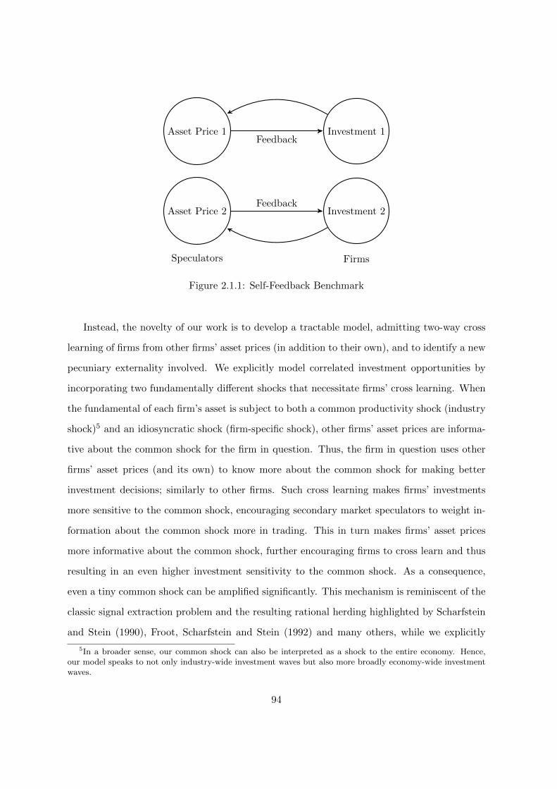
Asset Price 1Feedback

Feedback

Investment 1

Asset Price 2

Speculators

Investment 2

Firms

Figure 2.1.1: Self-Feedback Benchmark

Instead, the novelty of our work is to develop a tractable model, admitting two-way cross

learning of firms from other firms’ asset prices (in addition to their own), and to identify a new

pecuniary externality involved. We explicitly model correlated investment opportunities by

incorporating two fundamentally different shocks that necessitate firms’ cross learning. When

the fundamental of each firm’s asset is subject to both a common productivity shock (industry

shock)5 and an idiosyncratic shock (firm-specific shock), other firms’ asset prices are informa-

tive about the common shock for the firm in question. Thus, the firm in question uses other

firms’ asset prices (and its own) to know more about the common shock for making better

investment decisions; similarly to other firms. Such cross learning makes firms’ investments

more sensitive to the common shock, encouraging secondary market speculators to weight in-

formation about the common shock more in trading. This in turn makes firms’ asset prices

more informative about the common shock, further encouraging firms to cross learn and thus

resulting in an even higher investment sensitivity to the common shock. As a consequence,

even a tiny common shock can be amplified significantly. This mechanism is reminiscent of the

classic signal extraction problem and the resulting rational herding highlighted by Scharfstein

and Stein (1990), Froot, Scharfstein and Stein (1992) and many others, while we explicitly

5In a broader sense, our common shock can also be interpreted as a shock to the entire economy. Hence,our model speaks to not only industry-wide investment waves but also more broadly economy-wide investmentwaves.

94

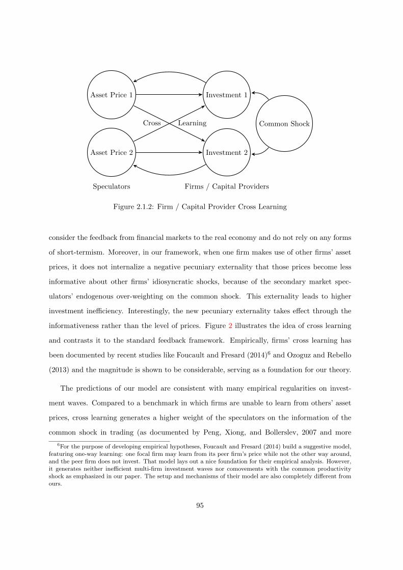
Asset Price 1

Cross Learning

Investment 1

Asset Price 2

Speculators

Investment 2

Firms / Capital Providers

Common Shock

Figure 2.1.2: Firm / Capital Provider Cross Learning

consider the feedback from financial markets to the real economy and do not rely on any forms

of short-termism. Moreover, in our framework, when one firm makes use of other firms’ asset

prices, it does not internalize a negative pecuniary externality that those prices become less

informative about other firms’ idiosyncratic shocks, because of the secondary market spec-

ulators’ endogenous over-weighting on the common shock. This externality leads to higher

investment inefficiency. Interestingly, the new pecuniary externality takes effect through the

informativeness rather than the level of prices. Figure 2 illustrates the idea of cross learning

and contrasts it to the standard feedback framework. Empirically, firms’ cross learning has

been documented by recent studies like Foucault and Fresard (2014)6 and Ozoguz and Rebello

(2013) and the magnitude is shown to be considerable, serving as a foundation for our theory.

The predictions of our model are consistent with many empirical regularities on invest-

ment waves. Compared to a benchmark in which firms are unable to learn from others’ asset

prices, cross learning generates a higher weight of the speculators on the information of the

common shock in trading (as documented by Peng, Xiong, and Bollerslev, 2007 and more

6For the purpose of developing empirical hypotheses, Foucault and Fresard (2014) build a suggestive model,featuring one-way learning: one focal firm may learn from its peer firm’s price while not the other way around,and the peer firm does not invest. That model lays out a nice foundation for their empirical analysis. However,it generates neither inefficient multi-firm investment waves nor comovements with the common productivityshock as emphasized in our paper. The setup and mechanisms of their model are also completely different fromours.

95

broadly by Rhodes-Kropf, Robinson and Viswanathan, 2005, Hoberg and Phillips, 2010, and

Bhattacharyya and Purnanandam, 2011) and the firms’ higher investment sensitivity to the

common shock.7 We further show that under cross learning, a firm’s investment and price

co-move more greatly with 1) other firms’ investments and prices, and with 2) the common

productivity shock as well, fitting in line with the evidence in Rhodes-Kropf, Robinson and

Viswanathan (2005), Pastor and Veronesi (2009), Hoberg and Phillips (2010), Bhattacharyya

and Purnanandam (2011) and Patton and Verardo (2012). We interpret these patterns as

higher systematic risks in industry-wide investment waves. Compared to alternative theories,

cross learning is further consistent with Maksimovic, Phillips and Yang (2013)’s message that

investment waves are more significant among public firms than among private firms, by high-

lighting the indispensable role of explicit prices in public financial markets. To the best of our

knowledge, our work is the first to establish the existence and significance of firms’ two-way

cross-learning effect on both investments, prices, and systematic risks.

Along this line, we investigate many circumstances in which the changes of economic con-

ditions generate higher systematic risks in investment waves via the cross-learning mechanism,

which are otherwise puzzling. First, an increasing uncertainty on the common productivity

shock, most typically induced by the introduction of major technological innovations, leads

to stronger weighting on the information of the common shock and higher systematic risks.

This is consistent with the empirical facts in Brunnermeier and Nagel (2004) and Pastor and

Veronesi (2006, 2009) and the more broadly documented evidence in the bubble literature

(Brunnermeier and Oehmke, 2013, Xiong, 2013). Our new mechanism contributes to the exist-

ing rational learning mechanisms (Pastor and Veronesi, 2009, Johnson, 2007), by featuring both

multi-firm investment waves and inefficiency. Second, an improvement of the firms’ knowledge

on the common productivity shock leads to higher systematic risks, consistent with the facts

in Greenwood and Nagel (2009). Last, lower market liquidity or higher variance of idiosyn-

cratic noisy supply also leads to higher systematic risks. These empirical regularities have

7Complementary to the theoretical literature that highlights investors’ attention allocation to the commonshock (see Peng and Xiong, 2006, Veldkamp, 2006, Veldkamp and Wolfers, 2007), our work speaks to its en-dogenous origin from firms’ cross learning as well as its feedback into firms’ investment decisions.

96

been frequently ascribed to separate behavioral accounts in the past literature, while our work

provides a consistent rational explanation.

Our framework allows for a clear welfare analysis, offering a new perspective to look at

the relationship between inefficient investment waves and industrial competition. Due to the

unaligned interests of firms and speculators in feedback and the new pecuniary externality

associated with cross learning, the investment waves are inefficient. In particular, we show that

as the number of firms in an industry increases, cross learning becomes stronger, leading to a

more severe pecuniary externality. This suggests a rationale for the puzzling facts identified

in Hoberg and Phillips (2010) and Greenwood and Hanson (2013) that more competitive

industries exhibit more predictable financial and real boom-bust cycles as well as greater market

and real inefficiencies. According to Hoberg and Phillips (2010), no single existing theory can

accommodate their findings. Our cross-learning mechanism with the new pecuniary externality

implies that more competitive industries may exhibit more over-weighting on the common

shock, more under-weighting on the idiosyncratic shocks, and more inefficient investment waves

with higher systematic risks, consistent with Hoberg and Phillips (2010) and Greenwood and

Hanson (2013)’s messages. Ozoguz and Rebello (2013) have also explicitly identified that

firms in more competitive industries have a higher investment sensitivity to stock prices of

their peers, which supports our predictions.

Fundamentally, the amplification effect of cross learning stems from a series of endogenous

strategic complementarities and a spiral that are absent in existing literature. At the begin-

ning, the dependence of investment on asset price results in an endogenous complementarity

between each firm’s investment sensitivity on the common shock and speculators’ weighting

on information about the common shock. When multiple firms’ cross learning is introduced,

a new spiral comes out. Cross learning first makes different firms’ investments more corre-

lated with the common shock as well as with each other. As a result, speculators find it

more profitable to put a higher weight on information about the common shock. Since asset

prices thus become relatively more informative about the common shock, firms’ investment

sensitivities on the common shock increase even more. This spiral further generates two new

97

complementarities in our multi-firm setting. The first is among speculators’ weights on the

information about the common shock in each asset market, and the second is among different

firms’ relative investment sensitivities to the common shock. The interaction of the spiral

and these endogenous complementarities is again seen in Figure 2, which constructs a strong

amplification effect from a fundamental shock to systematic risks. In contrast to the existing

literature involving complementarities in financial markets (see Veldkamp, 2011, for an exten-

sive review), our mechanism does not rely on any exogenous complementarities (for example,

higher-order beliefs or coordination in actions) but a well documented fact that firms learn

from own and other firms’ asset prices. Given that trading in financial markets usually exhibit

natural strategic substitutability, our endogenous complementarities and spiral are of more

significance.

Related Literature. Our work contributes to the literature of rational models on invest-

ment booms and busts.8 Early literature has focused on the role of industrial organizations (for

example, Reinganum, 1989, Jovanovic and McDonald, 1994) or self-fulfilling expectations (for

example, Shleifer, 1986) in generating investment waves, but financial markets are generally

absent in these classic papers. The modern literature has been paying increasing attention

to the role of learning in financial markets.9 In the rational learning model of Rhodes-Kropf

and Viswanathan (2004), which shares a similar signal extraction problem with ours, man-

agers cannot distinguish between common misvaluation and possible idiosyncratic synergies,

leading to merger and acquisition waves. Pastor and Veronesi (2009) propose a more explicit

learning model, in which the uncertain productivity of a new technology is subject to learn-

ing. Learning and the ensuing technology adoption makes the uncertainty from idiosyncratic

to systematic, generating investment waves. In this spirit, Johnson (2007) argues that firms

8This literature is more broadly related to the bubble and modern macro-finance literatures mainly based onbehavioral or belief aspects and agency or financial frictions, as discussed above. The focuses of those literaturesare however different from ours. Our model is not intended as a general dynamic theory of booms and bustseither.

9Other notable rational models on investment waves include DeMarzo, Kaniel, and Kremer (2007, 2008),featuring endogenous relative wealth concerns from the non-tradability of future endowments, Carlson, Fisherand Giammarino (2004) and Aguerrevere (2009), featuring investments as real options, and Ozdenoren andYuan (2013), featuring contractual externalities given the average performance contractable and the resultingexcessive risk-taking.

98

may learn about uncertain investment opportunities in the form of experimenting, which also

generates investment waves. Our contribution to this literature is three-fold. First, our model

features multiple firms and their cross learning explicitly, which allows us to study industry-

wide investment waves directly rather than to look at them from the perspective of single-firm

investment cycles. Second, we cast the microstructure of public asset markets explicitly by

an adapted Kyle (1985) model, ensuring us to reflect the indispensable role of public financial

markets as suggested by Maksimovic, Phillips and Yang (2013). Lastly, our model identifies

a new externality regarding the use of information about common shocks and idiosyncratic

shocks in making inefficient investment decisions.

Our framework also contributes to the burgeoning feedback literature as surveyed by Bond,

Edmans and Goldstein (2012). Among existing models, closely related are Goldstein, Ozde-

noren and Yuan (2013), Goldstein and Yang (2014a,b), and Sockin and Xiong (2014a,b), all of

which highlight the feedback from (secondary market) speculators’ information aggregation to

(primary market) capital providers’ scale-varying real investment decisions. Technically, these

papers have also employed a log-normal framework. Our contribution is to investigate multi-

firm feedback by introducing a tractable two-way cross-learning framework with two types of

shocks, which generates the new pecuniary externality and various implications that are absent

in existing models.

Identifying the externality associated with cross learning contributes to the large pecuniary

externality literature.10 The classical pecuniary externality takes effect through the level of

prices: agents do not internalize the impacts of their actions on equilibrium price levels, leading

to a welfare loss under various frictions. In our framework, instead, firms that make real

investment decisions do not fully internalize the impacts of cross learning on equilibrium price

informativeness. This leads to a “tragedy of the commons” regarding the use of the price

system as an information source under multi-firm cross learning. In this sense, our pecuniary

externality is reminiscent of the learning externality in the early dynamic learning and herding

literature (for example, Vives, 1997) that an agent, when responding to his private information,

10See Stiglitz (1982), Greenwald and Stiglitz (1986), Geanakoplos and Polemarchakis (1985), and Farhi andWerning (2013), He and Kondor (2013), Davila (2014) for recent theoretical developments.

99

does not take into account the benefit of increased informativeness of public information in the

future.11

Our work is also related to the literature on the interaction across asset markets or fun-

damentals, in particular the models that highlight learning. This literature has focused on

speculators’ learning rather than firms’ cross learning as we model. Cespa and Foucault (2014)

consider the contagion of illiquidity across segmented markets by introducing a concept of

cross-asset learning. By cross-asset learning, speculators trading in one market can potentially

learn from the asset price in another market, which generates propagation. Goldstein and

Yang (2014c) model an environment in which different speculators are informed of different

fundamentals affecting one single asset. Trading on information about the two fundamentals

exhibits complementarity, suggesting that greater diversity of information improves price in-

formativeness. Our model complements to those papers by focusing on the implications of firm

cross learning on both real investments and asset prices, in contrast to their exchange economy

setting that focuses on trading.

Finally, our framework is broadly related to a large macroeconomic literature focusing on

dispersed information, in particular on the different roles of private and public information.

Closely related are Angeletos, Lorenzoni and Pavan (2012) on the role of beauty contest in

generating investment exuberance and Amador and Weill (2010) on the crowding-out effect

of exogenous public information provision to the use of private information.12 Compared to

Angeletos, Lorenzoni and Pavan (2012) highlighting information spillover from real activities to

financial markets, our cross-learning framework with more detailed financial market structures

arguments it with the opposite learning channel explicitly. Importantly, by modeling cross

learning with two types of shocks, we are able to generate new strategic complementarities and

the new spiral towards the common shock, which are consistent with empirical evidence. Our

11The recent study of Vives (2014) further combines the classical pecuniary externality (through the level ofprices) and the learning externality associated with exogenous public information in an industrial competitioncontext. This is different from our new pecuniary externality through endogenous price informativeness on thetwo shocks. Its focus is also on the strategic interaction in product markets instead of our endogenous crosslearning in financial markets.

12Amador and Weill (2010) also relies on the earlier idea in Vives (1993) that the more informative pricesare, the less agents rely on private information, with the consequence that less information will be incorporatedinto prices.

100

externality is also different from theirs that features beauty contest in signaling and higher-

order uncertainties. Complementary to Amador and Weill (2010), the externality in our model

stems from a different mechanism and suggests a new crowding-out effect: endogenous over-

weighting of the common shock crowds out the use of information about the idiosyncratic

shocks. Neither of these two papers has distinguished between common productivity shock

and idiosyncratic productivity shocks.

The rest of the paper is organized as follows. Section 3.2 lays out the model, featuring

correlated investment opportunities and cross learning. Section 2.3 characterizes the cross-

learning equilibrium and benchmarks it to the self-feedback case. Section 2.4 investigates

important implications of cross learning with a focus on systematic risks in investment waves.

Section 2.5 explores the externality and the relationship between investment inefficiency and

competition. Section 2.6 discusses some extensions of the model. All proofs are delegated to

Appendix unless otherwise noted.

2.2 Model

2.2.1 Economy

The model extends the feedback framework of Goldstein, Ozdenoren and Yuan (2013) for a

different focus on capital provider cross learning.13 We consider a continuum of 1 of firms,

i ∈ [0, 1), each having an asset traded in a secondary market. Each firm i’s corresponding asset

market is occupied by a mass 1 of informed risk-neutral speculators, respectively. We index

speculators for firm i by a couple (i, j), with j ∈ [0, 1).14 Each firm i’s corresponding secondary

market is occupied by noise traders. Each firm also has an exclusive capital provider i in a

primary market who decides how much capital to provide to the firm for investment purpose.

13For related papers building on this framework or sharing a similar mathematical foundation in modeling,see Sockin and Xiong (2014a,b) and Goldstein and Yang (2014a,b). These papers do not consider fundamentallydifferent productivity shocks or multiple firms’ cross learning as we do.

14Since the speculators do not have a diversification motive, our results are unaffected if we assume that theycan trade all assets. In other words, market segmentation in terms of trading plays no roles in our model.

101

There are three dates, t = 0, 1, 2. At date 0, the speculators trade in their corresponding

asset market with their private information, and the asset price aggregates their information.

At date 1, the capital providers observe the asset prices of both their own firm and all the

other firms. Having observed all the prices and received their private information, the capital

providers decide the amount of capital to provide for their corresponding firms and the firms

undertake investment accordingly. All the cash flows are realized at date 2.

2.2.2 Capital Providers and Investment

All the firms in the economy have an identical linear production technology: Q(Ii) = AFiIi ,

where Ii is the amount of capital provided by capital provider i to firm i, and A and Fi are

two stochastic productivity shocks. Specifically, shock A captures an industry-wide common

productivity shock, and shock Fi captures the idiosyncratic productivity shock for firm i only.15

Denote by a and fi the natural logs of these shocks, and assume that they are normal and

mutually independent:

a ∼ N(0, 1/τa) , and fi ∼ N(0, 1/τf ) ,

where τa and τf are positive and i ∈ [0, 1).

The introduction of multiple firms and the two fundamentally different productivity shocks

plays an important role in necessitating firms’ cross learning. Specifically, if the investment

opportunities are uncorrelated, cross learning makes no sense. On the other hand, however,

if the investment opportunities are perfectly correlated, all asset prices become identical and

thus there is no need to learn from other’s prices as well. To flesh our cross-learning mechanism

out, we abstract away from possible industrial organization of the firms’ product market.

At date 1, all the capital providers choose the amount of capital Ii simultaneously in their

respective primary markets. Capital provider i captures a proportion κ ∈ (0, 1) of the output

Q(Ii) by providing Ii, which incurs a private quadratic adjustment cost, C(Ii) = 12cI

2i . Thus,

15In what follows, we omit the term productivity for brevity at times when there is no confusion.

102

capital provider i’s problem at t = 1 is

maxIi

E[κAFiIi −

1

2cI2i |Γi

], (2.1)

where Γi is the information set of capital provider i at t = 1. It consists of the price of firm i’s

own asset, Pi, and those of all the other firms’ assets, denoted by the set {P−i} for brevity,16

formed at date 0 as endogenous public signals, as well as their private signals about the (log)

productivity shocks a and fi. Specifically, we assume that each capital provider i gets a private

noisy and independent signal sa,i about the (log) common productivity shock a with precision

τs, and another private noisy and independent signal sf,i about its own (log) idiosyncratic

productivity shock fi with precision τf :

sa,i = a+ εa,i , where εa,i ∼ N(0, 1/τsa) , and

sf,i = fi + εf,i , where εf,i ∼ N(0, 1/τsf ) .

That is, for capital provider i, the information set is Γi = {Pi, {P−i}, sa,i, sf,i}.

Different from existing literature, one major novelty of our setup is to allow capital providers

to learn from other firms’ asset prices as well as own firms’ prices, which we formally call cross

learning. As will be highlighted later, although the capital providers only care about their own

firms, they use the prices of other firms’ assets for making better investment decisions.

2.2.3 Speculators and Secondary Market Trading

At date 0, the remaining cash flow (1−κ)Q(Ii), as an asset, is traded in a separate competitive

secondary market for each firm i. For firm i, denote the price of this asset by Pi. To focus on

capital providers’ cross learning, we do not consider any possible monetary transfers from the

secondary market to the firm, but highlight the information revealed in the secondary market

16As will be elaborated later, we focus on symmetric equilibria in which the firm in question i always puts thesame weight on each of other firms’ asset prices in cross learning. Thus, it is unnecessary for us to distinguishbetween those asset prices in analyzing cross learning.

103

trading.17 In the asset market of firm i, each speculator (i, j) has two private and independent

signals about the common shock and the respective idiosyncratic shock. Specifically, the first

signal is about the common shock:

xij = a+ εx,ij , where εx,ij ∼ N(0, 1/τx) ,

and the second signal is about the firm-specific idiosyncratic shock:

yij = fi + εy,ij ,where εy,ij ∼ N(0, 1/τy) .

Thus, the information set of speculator (i, j) is Γij = {xij , yij}.18

Based on their private information, the speculators submit limited orders in a similar

manner of Kyle (1985), with an additional constraint that each speculator can buy or sell up

to a unit of the asset.19 Formally, the speculators maximize their expected trading profit,

taking the asset price as given.20 Their problems at t = 0 are

maxdij∈[−1,1]

dijE [(1− κ)AFiIi − Pi|Γij ] , (2.2)

where dij is speculator (i, j)’s demand. The aggregate demand from the speculators in market

i is given by Di =∫ 10 dijdj.

We assume that the noisy supply in asset market i takes the following form:

∆(ζ, ξi, Pi) = 1− 2Φ(ζ + ξi − λ logPi) ,

17Hence, this asset can be interpreted as either equity of the firm or a derivative on the return from the firm’sinvestment. See a more detailed justification of this point in Goldstein, Ozdenoren and Yuan (2013).

18The fact that the speculators’ information set does not consist of the asset prices is not essential. For anyfirm i, even if its speculators can learn from its asset price Pi, as long as they do not cross learn from otherfirms’ asset prices {P−i}, all of our results are unaffected.

19As discussed in Goldstein, Ozdenoren and Yuan (2013), the specific size of this position limit is inessentialfor the results, as long as speculators cannot take unlimited positions, otherwise the prices will be fully revealing.This constraint can be easily justified by their capital or borrowing constraints.

20The asset price can be viewed as set by a unmodeled market maker, as that in Kyle (1985).

104

where

ζ ∼ N(0, τ−1ζ ) , and ξi ∼ N(0, τ−1ξ ) .

We elaborate the noisy supply. Φ(·) denotes the cumulative standard normal distribution

function. The first shock ζ captures a common noisy supply shock that can be viewed as

industry-wide sentiment or industry-wide fund flow. The second shock ξi captures the id-

iosyncratic noisy supply shock in market i that can be viewed as styled trading or uninformed

investors’ unobserved preferences. The presence of a common noisy supply not only makes our

framework more general, but more importantly prevents the aggregate price from fully reveal-

ing the common productivity shock. Both noisy supply shocks ζ and ξi are independent and

also independent of other shocks in the economy. Meanwhile, λ in the noisy supply function

captures price elasticity and can be viewed as market liquidity. When λ is high, the demand

from speculators can be easily absorbed and thus their aggregate demand has little impact on

the asset prices.

Finally, in equilibrium, the prices will clear each asset market by equalizing the aggregate

speculator demand to the noisy supply in each asset market i:

Di = ∆(ζ, ξi, Pi) . (2.3)

2.2.4 Discussion

Before proceeding, we discuss some important differences of our settings from the past literature

in the feedback literature, in particular, Goldstein, Ozdenoren and Yuan (2013), Foucault and

Fresard (2014), and the contemporaneous study by Goldstein and Yang (2014a,b). There are,

of course, more differences between our work and the existing feedback literature than what

we discuss below, but the following ones are crucial for our mechanism and thus help stand

out our contribution.

First, to lay out a foundation for characterizing cross learning, our model features a con-

tinuum of many firms. To accommodate multiple firms and two-way cross learning imposes

105

new technical challenges in the sense of finding closed form solutions. To this end, our model

provides a tractable approach not only suited for our purpose but potentially useful for future

work in other directions.

Second, built upon the multiple-firm setup, our economy features two fundamentally dif-

ferent productivity shocks: one is common to all firms while the other is firm-specific. In most

previous literature, there is only one productivity shock. One exception is Goldstein and Yang

(2014a,b) who consider two shocks on the cash flow. However, their two shocks are fundamen-

tally symmetric. Specifically, their two shocks differ in an exogenous informational sense that

the capital providers perfectly observe one but not the other. Instead, our model allows us to

explicitly recover how cross learning affects the endogenous sensitivities of firms’ investment

on the specific common shock and the idiosyncratic shocks. The contrast between the two

fundamentally different shocks plays an important role in generating investment waves as well

as delivering welfare implications on inefficient investment waves and competition.

Third, to highlight the interaction of the two fundamentally different shocks under cross

learning, our model does not feature any public information of the speculators as often seen in

the literature. Our efficiency implications come endogenously from a new pecuniary externality

absent in previous literature that focuses on coordination failure or higher-order beliefs.

Finally, in contrast to the hypotheses development in Foucault and Fresard (2014), our

framework features fully two-way cross learning instead of one-way learning by a focal firm

from its peer firm. The one-way learning channel in Foucault and Fresard (2014) gives clear

predictions on how the peer firm’s stock price may affect the focal firm’s investment, but the

peer firm itself does not invest or learn. Our framework with two-way cross learning as well as

more detailed real and financial market structures captures the new strategic complementarities

and spiral toward the common productivity shock. The fundamental difference between the

common shock and the idiosyncratic shocks matters only when the fully two-way cross learning

is introduced. This eventually generates industry-wide inefficient investment waves consistent

with empirical regularities.

106

2.3 Cross-Learning Equilibrium

2.3.1 Equilibrium Definition

We formally introduce the equilibrium concept. We focus on symmetric linear equilibria that

are standard in the literature. Specifically, the speculators in market i long one share of the

corresponding asset when φixij + yij > µi, and short one share otherwise, where φi and µi are

two constants that will be determined in equilibrium. Since agents are risk neutral and firms

are symmetric in our framework, symmetry further implies that φi = φ and µi = µ, which

mean that all the speculators use symmetric trading strategies in all asset markets, and the

information contents of all asset prices are also symmetric.

Definition 2.3.1. A (symmetric) cross-learning equilibrium is defined as a collection of a

price function for each firm i, Pi(a, fi, ζ, ξi): R4 → R, an investment policy for each capital

provider i, Ii(sa,i, sf,i, Pi, {P−i}): R2 × R∞ → R, and a linear monotone trading strategy for

each speculator (i, j), dij(xij , yij) = 1(φixij + yij > µi)− 1(φixij + yij 6 µi), such that

i) each capital provider i’s investment policy Ii(sa,i, sf,i, Pi, {P−i}) solves problem (2.1),

ii) each speculator (i, j)’s trading strategy dij(xij , yij) is identical and solves problem (2.2),

and

iii) market clearing condition (2.3) is satisfied for each market i.

2.3.2 Equilibrium Characterization

We characterize the equilibrium, featuring the capital providers’ cross learning. The equi-

librium is hard to solve and involves many fixed-point problems, so we follow a step-by-step

approach.

Step 1. We first solve for the price functions, which helps characterize the information

contents of prices from the capital providers’ perspective. We have the following lemma:

Lemma 2.3.1. The speculators’ trading leads to the following equilibrium price of each asset

107

i:

Pi = exp

φi

λ√τ−1x φ2i + τ−1y

a+1

λ√τ−1x φ2i + τ−1y

fi +ζ + ξiλ− µi

λ√τ−1x φ2i + τ−1y

. (2.1)

Hence, from any capital provider i’s perspective, the price for its own firm i’s asset is

equivalent to the following signal in predicting the common shock a:

za(Pi) =λ√τ−1x φ2i + τ−1y logPi + µi

φi= a+

1

φifi +

√τ−1x φ2i + τ−1y

φi(ζ + ξi) , (2.2)

and is equivalent to the following signal in predicting the corresponding idiosyncratic shock fi:

zf (Pi) = λ

√τ−1x φ2i + τ−1y logPi + µi = fi + φia+

√τ−1x φ2i + τ−1y (ζ + ξi) . (2.3)

Lemma 2.3.1 not only helps specify the information contents of a firm’s asset price to its

own capital provider, but also hints those to other firms’ capital providers. Thus, it suggests

the presence of capital providers’ cross learning when feasible. The next step formulates the

idea.

Step 2. We then characterize the informational consequences of cross learning. Specifically,

we show that, when cross learning is feasible, that is, capital provider i’s information set

includes both Pi and {P−i}, the capital provider relies on the aggregate price as well as the

own asset price (in addition to their own private signals) in inferring the two productivity

shocks. We impose the symmetry conditions φi = φ and µi = µ to conditions (2.1), (2.2) and

(2.3) now as we focus on symmetric equilibria, and we also define the aggregate price as

P =

∫ 1

0Pidi .

21

Lemma 2.3.2. For capital provider i, when her information set includes both Pi and {P−i},21The fact that the asset prices are equally weighted in calculating the aggregate price is inessential to their

information contents. Our results carry through even if we choose arbitrarily positive weights.

108

these asset prices are informationally equivalent to the following two signals:

i) a signal based on the aggregate price P :

za(P ) = a+

√τ−1x φ2 + τ−1y

φζ (2.4)

for predicting the common shock a, with the precision

τpa =τxτyτζφ

2

τx + τyφ2, (2.5)

which is increasing in φ, and

ii) a signal based on the own asset price Pi as well as the aggregate price P :

zf,i(P ) = zf (Pi)− φza(P ) = fi +

√τ−1x φ2 + τ−1y ξi (2.6)

for predicting the corresponding idiosyncratic shock fi, with the precision

τpf =τxτyτξ

τx + τyφ2, (2.7)

which is decreasing in φ.

Along with Lemma 2.3.1, Lemma 2.3.2 implies that cross learning changes the feedback

channel in which a capital provider uses asset prices to infer the two productivity shocks: she

now uses the aggregate price P to infer the common shock a and still uses the own price Pi

to infer the idiosyncratic shock fi. Intuitively, for capital provider i, other firms’ asset prices

{P−i} are uninformative on the idiosyncratic shock fi but informative on the common shock

a. Hence, when other firms’ asset prices are observable, which is natural in reality, the capital

provider of the firm in question uses them to make better inference about the common shock.

In particular, in a symmetric equilibrium, the aggregate price is sufficient for this purpose, as all

asset prices are symmetric. By the law of large numbers, P only aggregates information about

the common shock a: the information about idiosyncratic shocks and about the idiosyncratic

109

noisy supply shocks all gets wiped out, while the presence of the common noisy supply shock

still prevents the aggregate price from fully revealing. This makes za(P ), as characterized

in (2.4), the most informative signal about the common shock a the capital provider can

get. Moreover, knowing za(P ), the capital provider also eliminates the information about the

common shock and about the common noisy supply shock when she uses her own price Pi to

infer the idiosyncratic shock fi, as characterized in (2.6).

Step 3. We then solve for the capital providers’ optimal investment policy under cross

learning. This indicates the real consequences of cross learning. Lemma 2.3.2 implies that,

under cross learning, capital provider i uses the new signal za(P ) and her private signal sa,i to

infer the common shock a, and the new signal zf,i(P ) and the private signal sf,i to infer the

idiosyncratic shock fi. Thus, we have the following lemma.

Lemma 2.3.3. Observing sa,i, sf,i, Pi and {P−i}, capital provider i’s optimal investment policy

is

Ii =κ

cexp

[τsasa,i + τpaza(P )

τa + τsa + τpa+

1

2(τa + τsa + τpa)+τfsf,i + τpfzf,i(P )

τf + τsf + τpf+

1

2(τf + τsf + τpf )

].

(2.8)

The investment policy is intuitive. On the one hand, the optimal amount of investment is

higher when the share κ of capital provider is higher while lower when the investment cost c

is higher. On the other hand, the capital providers infer the two productivity shocks a and

fi independently but simultaneously in making investment decisions, reflected in the first and

third terms in the parenthesis. In particular, the capital providers find it optimal to learn

from both the own asset prices as well as other firms’ prices, which are summarized in the two

new signals za(P ) and zf,i(P ). This fits quite in line with the recent empirical facts about

firms’ and capital providers’ cross learning behavior (Foucault and Fresard, 2014, Ozoguz and

Rebello, 2013).

According to Lemma 2.3.3, we propose the following intuitive concept of investment sensi-

tivity to capture how the capital providers’ investment decision responds to the two produc-

tivity shocks under cross learning.

110

Definition 2.3.2. For capital providers, the investment sensitivity to the common productivity

shock and that to the idiosyncratic productivity shock are defined as:

Sa(τpa) =τsa + τpa

τa + τsa + τpa, and Sf (τpf ) =

τsf + τpfτf + τsf + τpf

,

respectively. We call Sa the common investment sensitivity and Sf the idiosyncratic investment

sensitivity henceforth.

We highlight that, the investment sensitivity depends on not only the capital providers’

private signals about the corresponding shock, but also the new endogenous price signals com-

ing from cross learning as characterized in Lemma 2.3.2. In particular, these two notions of

investment sensitivity are increasing functions of τpa and τpf , respectively, which are in turn

affected by the speculators’ trading strategy. Hence, by Lemma 2.3.2, we have the follow-

ing straightforward lemma that bridges the capital providers’ investment sensitivity and the

speculators’ weight φ on the signal of the common productivity shock.

Lemma 2.3.4. The common investment sensitivity Sa(τpa) is increasing in φ while the idiosyn-

cratic investment sensitivity Sf (τpf ) is decreasing in φ.

Lemma 2.3.4 is helpful because it offers an intuitive look at the real consequences of learning

from asset prices in the economy with two fundamentally different shocks. When speculators’

weight φ is higher, they put more weight on the information about the common shock, and

thus asset prices become more informative about the common shock while less informative

about the idiosyncratic shocks. This in turn leads to a more sensitive investment policy in

response to the common shock while a less sensitive one in response to the idiosyncratic shock.

Step 4. We finally close the model by solving for the speculators’ equilibrium trading strat-

egy, characterized by the weight φ and the constant µ. This also pins down other equilibrium

outcomes since they are all functions of φ.

For speculator (i, j), her expected profit of trading given her available information is

E [(1− κ)AFiIi − Pi|xij , yij ] , (2.9)

111

in which Ii and Pi have been characterized by conditions (2.8) and (2.1) respectively.

It is easy to show that, speculators’ expected profit (2.9) of trading asset i can be expressed

as

E [(1− κ)AFiIi − Pi|xij , yij ] =κ(1− κ)

cexp (α0 + α1xij + α2yij)− exp (γ0 + γ1xij + γ2yij) ,

where α0, α1, α2, γ0, γ1, and γ2 are all functions of φ:

α1 = (Sa + 1)τx

τa + τx,

α2 = (Sf + 1)τy

τf + τy,

γ1 =φ

λ√τx + τyφ2

τxτa + τx

,

γ2 =1

λ√τx + τyφ2

τyτf + τy

.

By definition, in a symmetric cross-learning equilibrium with cross learning, we have

φ =α1 − γ1α2 − γ2

.

Plugging in α1, α2, γ1 and γ2 yields

φ =

(Sa + 1− φ

λ√τx+τyφ2

)τx

τa+τx(Sf + 1− 1

λ√τx+τyφ2

)τy

τf+τy

. (2.10)

Analyzing this equation by further plugging in Sa and Sf , which are both functions of φ, we

reach a unique cross-learning equilibrium, formally characterized by the following proposition.

Proposition 2.3.1. For a high enough noisy supply elasticity λ, there exists a cross-learning

equilibrium in which the speculators put a positive weight φ > 0 on the signal of the common

productivity shock. For a high enough information precision τy (of the speculators’ signal on

the idiosyncratic shock), the equilibrium is unique.

112

To establish the existence of a unique equilibrium is essential for our further analysis regard-

ing investment waves, as it allows us to investigate that how changes in economic environment

affect investments and prices through the cross-learning mechanism. When φ is higher, the

speculators put more weight on the information about the common shock in trading, encour-

aging all the capital providers to respond to the common shock more sensitively through cross

learning, which in turn leads to an even higher φ. This new spiral gives rise to many impli-

cations in line with the empirical phenomena regarding industry-wide investment waves as we

explore later.

The conditions to guarantee a unique cross-learning equilibrium are not only standard in

the feedback literature (see Goldstein, Ozdenoren and Yuan, 2013, among many others) but

empirically plausible. A relatively high noisy supply elasticity λ implies that markets are liquid

enough. A relatively high information precision τy of the speculators’ signal on the idiosyncratic

shock suggests that asset market participants understand their target firms better than the

whole industry. These two conditions are in particular appropriate when we focus on the

contexts leading to investment waves: relatively liquid markets and relatively more uncertain

macroeconomic news.22,23

2.3.3 Self-Feedback Benchmark

Having established the existence and uniqueness of a cross-learning equilibrium, we benchmark

the cross-learning equilibrium to the corresponding self-feedback equilibrium in a comparable

economy. This self-feedback benchmark helps understand how the presence of cross learning

affects the capital providers’ investment policy and the speculators’ trading strategy, in contrast

to the counterfactual where cross learning is absent. In demonstrating these effects, we again

focus on the difference of the speculators’ weight φ on the signal of the common productivity

shock in the two respective equilibria, as all equilibrium outcomes are functions of this weight.

22In the appendix, we explore other sufficient conditions that guarantee a unique cross-learning equilibrium.Our results regarding investment waves and investment inefficiency survive under other sets of sufficient condi-tions.

23We have numerically shown that these conditions are not restrictive. Even for reasonably small λ and τy,our model still features a unique cross-learning equilibrium. These numerical results are reported in Section 2.5.

113

We still consider unique symmetric equilibria and denote by φ′ the speculators’ weight on the

signal of the common productivity shock in the self-feedback benchmark.

Formally, the only difference of the benchmark economy is that, each capital provider

i observes its own asset price Pi but not other firms’ asset prices {P−i}. That is, capital

provider i’s information set is Γi = {Pi, sa,i, sf,i}. We have

Pi = exp

φ′

λ√τ−1x (φ′)2 + τ−1y

a+1

λ√τ−1x (φ′)2 + τ−1y

fi +ζ + ξiλ− µi

λ√τ−1x (φ′)2 + τ−1y

,

which is equivalent to the following two signals

za(Pi) =λ√τ−1x (φ′)2 + τ−1y logPi + µi

φ′= a+

1

φ′fi +

√τ−1x (φ′)2 + τ−1y

φ′(ζ + ξi)

in predicting the common shock a and

zf (Pi) = λ

√τ−1x (φ′)2 + τ−1y logPi + µi = fi + φ′a+

√τ−1x (φ′)2 + τ−1y (ζ + ξi)

in predicting the corresponding idiosyncratic shock fi. The precisions of za(Pi) and zf (Pi) are

denoted as τpa and τpf where

τpa =1

1(φ′)2 τ

−1f +

τ−1x (φ′)2+τ−1

y

(φ′)2 (τ−1ζ + τ−1ξ ),

and

τpf =1

(φ′)2τ−1a + (τ−1x (φ′)2 + τ−1y )(τ−1ζ + τ−1ξ ).

Following the same definition of investment sensitivity and the same analysis for the capital

114

providers’ investment policy and the speculators’ trading strategy, we have

S′a =τsa + τpa

τa + τsa + τpa+

τpfτf + τsf + τpf

φ′ ,

S′f =τsf + τpf

τf + τsf + τpf+

τpaτa + τsa + τpa

1

φ′,

α′1 =(S′a + 1

) τxτa + τx

,

α′2 =(S′f + 1

) τyτf + τy

,

γ′1 =φ′

λ√τx + τy(φ′)2

τxτa + τx

,

γ′2 =1

λ√τx + τy(φ′)2

τyτf + τy

.

In the self-feedback equilibrium, we also have

φ′ =α′1 − γ′1α′2 − γ′2

to pin down the speculators’ weight on the information of the common shock. Plugging in

α′1, α′2, γ′1 and γ′2 yields

φ′ =

(S′a + 1− φ′

λ√τx+τy(φ′)2

)τx

τa+τx(S′f + 1− 1

λ√τx+τy(φ′)2

)τy

τf+τy

. (2.11)

Therefore, we have the following proposition regarding the comparison between the cross-

learning equilibrium and the corresponding self-feedback benchmark. We focus on comparable

cases in which a self-feedback equilibrium and its corresponding cross-learning equilibrium are

both unique.

Proposition 2.3.2. For a high enough noisy supply elasticity λ, a low enough idiosyncratic

noisy supply shock precision τξ, and a high enough information precision τy (of the specula-

tors’ signal on the idiosyncratic shock), there exists a unique self-feedback equilibrium in which

speculators put a positive weight φ′ > 0 on the signal of the common productivity shock. In

115

particular, φ′ < φ, where φ is the speculators’ weight on the signal of the common productivity

shock in the corresponding cross-learning equilibrium.

The comparison between a cross-learning equilibrium and its corresponding self-feedback

equilibrium implies that, the presence of cross-learning may encourage the speculators to put

a higher weight φ on the information about the common productivity shock. We also have

the following straightforward corollary regarding the information precisions of the endogenous

price signals and the capital providers’ investment sensitivities, all of which are functions of φ.

Corollary 2.3.1. Compared to its corresponding self-feedback equilibrium, a cross-learning

equilibrium features a higher ratio of the asset price information precision in predicting the

common shock to that in prediction the idiosyncratic shock, i.e., τpa/τpf > τpa/τpf , and a

higher ratio of the investment sensitivity to the common shock to that to the idiosyncratic

shock, i.e., Sa/Sf > S′a/S′f .

The results in Proposition 2.3.2 and Corollary 2.3.1 uncover the informational and real

consequences of cross learning in equilibrium. Intuitively, when the capital providers are able

to cross learn from each other’s asset prices (in addition to their own firms’ prices), they

indeed do so in equilibrium as other firms’ asset prices help them better infer the common

shock. This makes firms’ investments relatively more correlated with the common shock as

well as with each other. Thus, the speculators find it more profitable to put more weight on

the information about the common shock. This further makes asset prices becoming relatively

more informative about the common shock in guiding investment decisions, and thus the capital

providers respond to the common shock even more sensitively in investing. This spiral is absent

in existing feedback models, and it indeeds plays an important role in amplifying industry-wide

investment waves as we fully explore in the next section.

116

2.4 Systematic Risks in Investment Waves

The most important implications of cross learning are on the systematic risks in industry-

wide investment waves. This comes from the endogenous spiral between the capital providers’

investment sensitivity to the common shock and the speculators’ weighting on the information

about the common shock, as shown in Section 2.3. In our multi-firm setting, this spiral

further leads to two new endogenous strategic complementarities. The new spiral and strategic

complementarities help generate empirical implications of systematic risks in many relevant

economic environments that seem jointly puzzling otherwise.

2.4.1 Impacts of Speculators’ Weight on Systematic Risks

It is instructive to first investigate the impacts of the speculators’ weight φ (on the information

of the common shock) on systematic risks, taking the weight as given. Along the way, we also

introduce our measures of systematic risks in investment waves.

Definition 2.4.1. The correlation coefficients between the investments of two firms and be-

tween the asset prices of two firms are defined as:

βI =Cov(log Ii, log Ij)√

Var(log Ii)√

Var(log Ij), and βP =

Cov(logPi, logPj)√Var(logPi)

√Var(logPj)

,

respectively. We call βI the investment beta and βP the price beta henceforth.

We take the investment beta βI and the price beta βP as two major measures of systematic

risks in investment waves, on both the real and financial aspects, respectively. Typically,

stronger investment waves are associated with a higher βI and a higher βP . However, as the

recent study by Hong and Sraer (2013) argues, some investment waves only exhibit a higher

investment beta βI but not a higher price beta βP . Hence, it is helpful to us to distinguish

between these two betas in characterizing different types of investment waves.

We have the following intuitive result on the impacts of the speculators’ weight φ on the two

betas. When the speculators put a higher weight on the information of the common shock, the

117

capital providers’ investment sensitivities to the common shock increases, which makes their

investments more correlated. Moreover, this in turn encourages the speculators to put a higher

weight on the common productivity shock, which results in a higher correlation between asset

prices. With the comparison between a cross-learning equilibrium and its corresponding self-

feedback equilibrium in Section 2.3, these predictions shed lights on the empirical regularities in

papers such as Rhodes-Kropf, Robinson and Viswanathan (2005), Pastor and Veronesi (2006,

2009), Hoberg and Phillips (2010), Bhattacharyya and Purnanandam (2011) and Patton and

Verardo (2012).

Lemma 2.4.1. Both the investment beta βI and the price beta βP are increasing in φ when

φ > 0.

Similarly, we also look at the correlations between investment and the two productivity

shocks, respectively. As a complement to Definition 2.3.2 of investment sensitivity and the

associated Lemma 2.3.4, the following definition shoots a closer look at the equilibrium invest-

ments’ correlation with the two shocks.

Definition 2.4.2. The correlation coefficient between investment and the common productivity

shock and that between investment and the idiosyncratic productivity shock are defined as:

βA =Cov(log Ii, logA)√

Var(log Ii)√

Var(logA), and βF =

Cov(log Ii, logFi)√Var(log Ii)

√Var(logFi)

,

respectively. We call βA the common investment correlation and βF the idiosyncratic invest-

ment correlation henceforth.

Intuitively, when the speculators put a higher weight on the information of the common

shock, both investments and prices become more correlated with the common productivity

shock instead of the idiosyncratic shocks. This is because the asset prices become more in-

formative in predicting the common shock but less informative in predicting the idiosyncratic

shock.

Lemma 2.4.2. The common investment correlation βA is increasing in φ while the idiosyncratic

118

investment correlation βF is decreasing in φ when φ > 0.

In what follows, we focus on the investment beta βI and the price beta βP in exploring

the full equilibrium dynamics, highlighting the speculators’ endogenous weight and equilibrium

systematic risks under cross learning. The investigation on the common investment correlation

βA and the idiosyncratic investment correlation βF yields the same insights.

2.4.2 Endogenous Cross Learning and Systematic Risks

Having established the impacts of the speculators’ weight φ (on the information about the

common shock) on systematic risks, we turn to one of the most interesting parts of the paper,

which investigates how the changes of economic environments affect equilibrium systematic

risks through the cross-learning mechanism. This unifies several empirical regularities that are

otherwise hard to reconcile without taking the capital providers’ cross learning into account.

Mathematically, we perform formal comparative statics of the equilibrium betas with respect to

exogenous parameters. We elaborate the first comparative statics (with respect to the common

uncertainty) in more detail to explore the underlying mechanism, and the other comparative

statics will follow the same intuition.

Common Uncertainty

We first focus on the effects of common uncertainty, which is captured by the prior precision τa

of the common productivity shock. We view the change of common uncertainty as an important

case, because a majority of industry-wide and economy-wide investment waves is associated

with an increasing common uncertainty at the first place. The most typical driver for an

increasing common uncertainty is the arrival of all-purpose technology or financial innovations,

as documented in Brunnermeier and Nagel (2004), Pastor and Veronesi (2006, 2009), and more

broadly the literature of bubbles. Our predictions help deliver a new perspective to look at the

impacts of innovations and the accompanying increasing common uncertainty on the systematic

risks in investment waves, highlighting the cross-learning mechanism.

119

We use the following assumption (only valid in this subsection on common uncertainly) to

flesh out the cross-learning mechanism.

Assumption 2.4.1. The ratios τsa/τa (of the capital providers’ signal precision on the common

shock and the prior precision on the common shock) and τx/τa (of the speculators’ signal

precision on the common shock and the prior precision on the common shock) are kept as

constants when τa changes.

Assumption 2.4.1 not only helps shut down a direct information channel that confounds the

cross-learning mechanism (only in this case about common uncertainty) but also captures the

reality better. By keeping the two ratios constant, both the capital providers and the specula-

tors do not find their private information more valuable in predicting the common productivity

shock. This is actually closer to the reality that, when the common uncertainty increases, no

market participant naturally has an advantage in resolving the common uncertainty. In this

case, our cross-learning mechanism plays an important amplification role that is impossible

otherwise. Assumption 2.4.1 is also completely benign; our results are only stronger without

it.

Lemma 2.4.3. Increasing the common uncertainty leads to a higher weight of the speculators

on the information about the common shock. Specifically, the speculators’ weight φ is decreasing

in τa.

From Lemma 2.4.3, we understand that an increasing in the common uncertainty leads

to a stronger cross-learning spiral towards the common shock, despite that both the capital

providers and speculators experience equally increasing uncertainty in their private informa-

tion on the common shock. The following proposition further establishes the impacts on the

equilibrium systematic risks.

Proposition 2.4.1. Increasing the common uncertainty leads to both a higher investment beta

and a higher price beta in equilibrium. Specifically, βI and βP are both decreasing in τa. We

120

further decompose the effects into two negative components (the same for βI and βP ):

dβ(τa, φ)

dτa=

∂β(τa, φ)

∂τa︸ ︷︷ ︸Mechanical Effect <0

+∂β(τa, φ)

∂φ

∂φ

∂τa︸ ︷︷ ︸Cross-Learning Effect <0

< 0 .

Proposition 2.4.1 indicates two effects contributing to the higher systematic risks associ-

ated with an increasing common uncertainty. The first is a mechanical effect that does not

depend on the endogenous interaction between the capital providers and the speculators under

cross learning. Intuitively, when the common uncertainty increases, speculators’ investment

sensitivity to the common shock increases as well. This immediately results in a higher corre-

lation among firms’ investments and prices. Figure 2.4.1 illustrates this mechanical effect in a

two-firm example.

Figure 2.4.1: Mechanical Effect on Systematic Risks

The second effect, the cross-learning effect, is more interesting and only at play in our multi-

firm cross-learning framework with two types of shocks. It reflects the new spiral between the

capital providers’ investment sensitivity to the common shock and the speculators’ weight on

the signal of the common shock. Interestingly, it takes place even when only some (not all)

firms in the economy perceive the increasing common uncertainty.24 Figure 2.4.2 illustrates

this cross-learning effect in a two-firm example. Suppose, without loss of generality, firm 1’s

24Technically, this requires some non-meaure-zero firms to perceive the increasing common shock.

121

capital provider perceives the increasing common uncertainty. As in the upper-left panel, firm

1’s investment sensitivity to the common shock Sa1 first increases (along with a decreasing

investment sensitivity to its idiosyncratic shock), leading to a higher weight φ1 on the infor-

mation of the common shock by its speculators. Then, as in the upper-right panel, a higher φ1

results in an even higher Sa1 since firm 1 learns from its own price. More importantly, because

of cross learning, firm 2’s investment sensitivity to the common shock Sa2 also increases, since

firm 2 finds firm 1’s price more informative about the common shock and thus understands

the common shock better. It then naturally leads to a higher weight φ2 on the information

of the common shock by firm 2’s speculators, as in the lower-left panel. Finally, the increase

of φ2 results in even higher Sa1 and Sa2 by cross learning, as in the lower-right panel. The

entire process suggests two new strategic complementarities only under cross learning: the first

is among speculators’ weights on the information about the common shock in each market,

and the second is among different firms’ relative investment sensitivities to the common shock.

With the two strategic complementarities, the spiral goes on and on and eventually pushes the

economy to a new equilibrium with much higher systematic risks.

Our predictions on systematic risks after an increasing common uncertainty are consis-

tent with the literature (Brunnermeier and Nagel, 2004, Pastor and Veronesi, 2006, 2009)

that documents the increasing systematic risks after major technological innovations, as these

innovations often come with industry-wide uncertain market prospects. In particular, the

cross-learning effect sheds lights on the huge magnitude of systematic risks in these investment

waves that are often ascribed to behavioral biases (see Brunnermeier and Oehmke, 2013, Xiong,

2013, for surveys).

Capital Providers’ Access to Information

We then turn to the capital providers’ access to private information, captured by the two

precisions τsa and τsf regarding the two productivity shocks, respectively. Again, we have the

following lemma pertaining to the speculators’ endogenous weight.

Lemma 2.4.4. Increasing the capital providers’ information precision on the common shock

122

leads to a higher weight of the speculators on the information about the common shock, while

increasing the capital providers’ information precision on the idiosyncratic shock leads to a

lower weight. Specifically, the speculators’ weight φ is increasing in τsa while decreasing in τsf .

Lemma 2.4.4 prescribes that, when the capital providers have better information on the

common shock, the equilibrium cross-learning spiral towards the common shock is also stronger;

while better information on the idiosyncratic shock pushes the cross-learning spiral towards the

idiosyncratic shocks. This further leads to the following proposition. Similar to Proposition

2.4.1, we have the mechanical effect and the cross-learning effect, both in the same direction.

Proposition 2.4.2. For the capital providers’ access to private information, we have the

following results.

i) Increasing the precision on the common shock leads to a higher investment beta when the

precision is not large, and always a higher price beta; specifically, βI is increasing in τsa when

τsa > τa + τxτζ and βP is always increasing in τsa.

ii) Increasing the precision on the idiosyncratic shock leads to both a lower investment beta

and a lower price beta; specifically, βI and βP are always decreasing in τsf .

The predictions here are broadly supported by the empirical evidence in Greenwood and

Nagel (2009). It suggests that younger and more confident capital providers, who tend to

have better knowledge about the industry-wide common shock compared to that on their

idiosyncratic shocks, tilt their investments more towards the common shock, leading to higher

investment and price correlations. Greenwood and Nagel (2009) admit that the magnitude of

systematic risks they have observed is obviously larger than any existing rational models can

accommodate and thus refer to behavioral explanations. In this sense, our predictions provide

a new angle to investigate such effects from a rational perspective, highlighting the potential

of strong cross learning.

123

Liquidity Trading

We also investigate the effects of liquidity trading, captured by the market liquidity λ and the

two precisions of noisy supplies τζ and τξ. Similarly, we have the following intuitive lemma on

the speculators’ endogenous weight.

Lemma 2.4.5. For liquidity trading, a higher weight of the speculators on the information

about the common shock results from a lower market liquidity, a lower variance of common

noisy supply, or a higher variance of idiosyncratic noisy supply. Specifically, the speculators’

weight φ is decreasing in λ, increasing in τζ , and decreasing in τξ.

The predictions along the three dimensions are all intuitive. When the market liquidity

is higher, it is easier for the noisy traders to absorb speculators’ demand, so that the cross-

learning spiral towards the common shock is weaker. When the variance of the common noisy

supply is lower, speculators are more likely to trade upon the common productivity shock.

In contrast, when the variance of the idiosyncratic noisy supply is lower, speculators are less

likely to trade upon the common shock, which results in a weaker spiral towards the common

shock,

These predictions are further reflected in the following proposition, speaking to the overall

effects of liquidity trading on investment waves. Again, similar to Proposition 2.4.1, we have

the mechanical effect and the cross-learning effect in the same direction.

Proposition 2.4.3. For liquidity trading, we have the following results.

i) A higher investment beta βI results from a lower market liquidity, a lower variance of

common noisy supply, or a higher variance of idiosyncratic noisy supply. Specifically, βI is

decreasing in λ, increasing in τζ , and decreasing in τξ.

ii) A higher price beta βP results from a lower market liquidity, or a higher variance of

idiosyncratic noisy supply. Specifically, βP is decreasing in λ and decreasing in τξ.

124

2.5 Investment Inefficiency and Competition

An important question is that how firms’ cross learning affects real investment efficiency. On

the positive side, cross learning allows capital providers to take advantage of more information

that would not be available if they were not able to observe their own and other firms’ asset

prices. However, the interests between capital providers and speculators in learning the two

types of shocks are not perfectly aligned. More importantly, each firm’s cross learning further

creates a new pecuniary externality on other firms. These frictions result in investment in-

efficiency. In particular, the pecuniary externality associated with cross learning increases in

the number of firms, suggesting that more competitive industries may exhibit more inefficient

investment waves.

In evaluating that how these frictions affect investment efficiency, we proceed by two steps.

First, we evaluate the overall investment efficiency and show that any cross-learning equilibrium

always features investment inefficiency. Then we characterize the new pecuniary externality

induced by cross learning to better understand the origin of such inefficiency. By doing this, we

particularly underscore the implications of competition on inefficient investment waves through

the new pecuniary externality.

2.5.1 Overall Investment Efficiency

Formally, we define investment efficiency by the ex-ante expected net benefit of the total

investments by all the firms, given that capital providers may learn from all publicly available

asset prices:

Definition 2.5.1. The investment efficiency of the economy is defined as

R =

∫ 1

0Ridi ,

where

Ri = E[E[AFiIi −

c

2I2i |Γi

]]

125

denotes each firm i’s ex-ante expected net benefit of investment, given its capital provider’s

information set under cross learning: Γi = {Pi, {P−i}, sa,i, sf,i}.

We have the following proposition indicating the universal presence of investment ineffi-

ciency in a cross-learning equilibrium. We focus on the cases in which a unique cross-learning

equilibrium is guaranteed.

Proposition 2.5.1. There always exists a unique optimal weight φ∗ > 0 of the speculators

on the signal of the common shock that maximizes investment efficiency. In particular, for

a high enough noisy supply elasticity λ and a high enough information precision τy (of the

speculators’ signal on the idiosyncratic shock), the optimal weight is always smaller than that

in the corresponding cross-learning equilibrium, i.e., φ∗ < φ.

Proposition 2.5.1 indicates that when the speculators’ signal on the idiosyncratic shock is

relatively more precise, they tend to put an inefficiently high weight on the other signal about

the common shock. This makes capital providers to respond to the common shock inefficiently

too sensitively, leading to inefficient investment waves. This particular inefficiency fits quite

in line with what we have observed in typical investment waves (for example, Rhodes-Kropf,

Robinson and Viswanathan, 2005, Peng, Xiong, and Bollerslev, 2007, Hoberg and Phillips,

2010, Bhattacharyya and Purnanandam, 2011) that both primary and secondary market in-

vestors pay inefficiently too much attention to common shocks or noisy macroeconomics news

while ignore informative idiosyncratic news.25

To better understand the impacts of cross learning on investment efficiency and potentially

shed lights on corrective policies, we perform comparative statistics of investment efficiency

with respect to several economic parameters. Again, we focus on unique cross-learning equi-

libria by assuming that the noisy supply elasticity λ and the information precision τy (of

speculators’ signal on the idiosyncratic shock) are high enough.

25Our framework is in fact general enough to admit the opposite case: when the speculators’ signal on thecommon shock is relatively more precise, they tend to put an inefficiently too high weight on the signal aboutthe idiosyncratic shocks, also leading to generic investment inefficiency. This case is empirically less plausible,but we still explore the theoretical possibilities in the appendix.

126

Proposition 2.5.2. In a cross-learning equilibrium, investment efficiency is higher when the

market liquidity is higher, or the precision of idiosyncratic noisy supply is higher, or the capital

providers’ information precision on the idiosyncratic productivity shock is higher. Specifically,

R is increasing in λ, τξ, and τsf .

The comparative statics regarding the investment efficiency are intuitive. First, a higher

market liquidity has a corrective effect on the investment efficiency. That is, in a deeper asset

market, the speculators’ trading positions can be more easily absorbed. Specifically, when an

asset market is more liquid or deeper, it becomes harder for the same amount of informed

trading to impact the asset price. This is in particular beneficial when cross learning is strong

after the arrival of major innovations or other common news involving high uncertainty, because

the inefficient impact from speculators’ overuse of information about the common shock can

be better absorbed.

Importantly, this corrective effect on real investment efficiency helps justify recent regula-

tory concerns and practices by the SEC in limiting informed speculators’ trading positions but

at the same time lifting the participation barrier to less informed market makers and retail

investors. These two are hard to be reconciled as approaches to correct investors’ irrationality

or to sidestep limits to arbitrage. In this sense, our cross-learning mechanism does a better

job in delivering policy implications than typical models featuring bubbles.

Second, increasing investment efficiency in an economy with cross learning calls for a better

use of information about the idiosyncratic shocks in the economy. Any policies on financial

disclosure or government communication failing to keep this point in mind may end up crowding

out the idiosyncratic news and resulting in investment inefficiency. This policy implication fits

broadly in line with the recent studies that speak to the dark side of financial disclosures or

central bank communications (Di Maggio and Pagano, 2013, Kurlat and Veldkamp, 2013).

Theoretically, the endogenous overuse of information on the common shock due to multi-firm

cross learning results in an inefficient crowding-out effect on the use of information on the

idiosyncratic shock. Thus, it also complements the idea on the crowding-out effect of public

information provision on the use of private information (see Amador and Weill, 2010).

127

2.5.2 Competition and Cross Learning

To help better understand the origin of investment inefficiency, we perform a theoretical exercise

to further identify a new pecuniary externality induced by cross learning. In particular, in

doing so, we extend our baseline model to admit finite number of firms. This allows us not

only to underscore the efficiency change associated with different extent of cross learning but

to investigate the relationship between competition and inefficient investment waves, which has

been a well documented puzzle in recent empirical literature (see Hoberg and Phillips, 2010,

Greenwood and Hanson, 2013, among others).

We first outline the extended cross-learning framework. A major challenge in identifying

the externality associated with cross learning is to deal with the information endowment effect.

Specifically, when the actual number of firms increase, the total amount of information in the

economy also increases, leading to an efficiency gain to each firm. This information endowment

effect confounds the identification of externalities and thus needs to be controlled properly. To

achieve this goal, our extended cross-learning framework still features a continuum of 1 of

firms being able to learn from all asset prices. However, we assume that the speculators do not

fully internalize capital providers’ cross learning. Concretely, they believe that each firm only

observes and learns from as many as n > 1 asset prices, including its own price. This setting

delivers an equilibrium weight (of the speculators on the information about the common shock)

identical to that in a corresponding economy with n finite firms operating and the speculators

fully internalizing their cross learning, while keeps the total amount of information endowment

invariant with n. Hence, we are able to stand out the externality associated with cross learning

as the number of firms increases.

We rigorously formulate the idea above as follows. We divide all the firms into n > 1

groups, a continuum of 1/n of firms in each group. The firms still observe and learn from all

the asset prices as in the baseline model, regardless of the grouping. However, the speculators

do not fully internalize firms’ cross learning as before. Specifically, let i ∈ [0, 1/n) denote

one firm in the first group. The speculators believe that for any i, the n firms in the set

128

{i + k/n|0 6 k 6 n − 1, k ∈ Z} learn only from the asset prices of each other but not from

the asset prices of other firms outside the set. Figure 5 offers an illustration of the case when

n = 3, in which the speculators believe that the three red firms (i, i+ 1/3, and i+ 2/3) cross

learn only from each other and the three blue firms (i′, i′ + 1/3, and i′ + 2/3) cross learn only

from each other, similar for other firm triples.

This setting has several advantages, both economically and technically. First, it casts in-

dustry competition in a straightforward way. Since the speculators are risk neutral, it looks to

them as if there are exactly n firms operating in the economy. Thus, the speculators’ weight in

equilibrium is identical to that in a corresponding economy with exactly n firms and the specu-

lators fully internalizing their cross learning. Second, it helps identify the pecuniary externality

induced by cross learning while keeps the total information endowment fixed. Especially, the

efficiency change associated with cross learning takes place only through the speculators’ en-

dogenous weighting over the two types of shocks, making it possible to distinguish that from

firms’ actual information endowment. Last, this setting offers a smooth transition between the

baseline model with full cross learning (as n goes to infinity) and the self-feedback benchmark

(as n equals to 1). This not only makes our analysis analytically tractable but helps unify all

the results and intuitions.

We acknowledge again that we are abstracting away from any possible industrial organiza-

tion of the firms’ product markets. Rather, we make use of the number of firms as a proxy for

competition, which we believe is the most relevant measure.26 This allows us to underscore

the cross-learning mechanism by highlighting it as the only interaction among firms. In this

sense, our model serves as a benchmark for further research that may take more aspects of

industrial competition along with firms’ cross learning into account.27

We proceed to characterize the equilibrium in the extended framework and the corre-

26To use the number of firms to proxy competition is common in the literature, especially when informationis a focus (see Vives, 2010, for a survey).

27For example, Peress (2010) offers an interesting analysis on the impacts of monopolistic competition inproduct markets on stock market efficiency, but does not consider feedback to real investments or cross learningas we do. He does not consider the implications on investment waves as well.

129

sponding investment efficiency. We still consider symmetric equilibria, and denote by φn the

speculators’ weight on the signal of the common shock, when the speculators believe that each

firm only learns from as many as n asset prices, including its own. For convenience, we call

the associated equilibrium an n-learning equilibrium.

Formally, each capital provider i still observes its own asset price Pi and all other firms’

asset prices {P−i}. Same as before, the information content of any asset price is characterized

by

Pi = exp

φn

λ√τ−1x φ2n + τ−1y

a+1

λ√τ−1x φ2n + τ−1y

fi +ζ + ξiλ− µi

λ√τ−1x φ2n + τ−1y

,

equivalent to a signal

zn (Pi) = φna+ fi +

√τ−1x φ2n + τ−1y (ζ + ξi) .

However, in an n-learning equilibrium, the speculators believe that each capital provider

only learns from its own price as well as the other n− 1 firms’ asset prices. Specifically, from

the speculators’ perspective, due to symmetry, each capital provider i has four signals: the

own private signals sa,i and sf,i, the signal zn(Pi) from its own asset price, and another signal

zn(P−i) coming from the other n− 1 asset prices:28

zn (P−i) = φna+

∑l 6=i fl

n− 1+

√τ−1x φ2n + τ−1y

(ζ +

∑l 6=i ξl

n− 1

).

From the speculators’ perspective, capital provider i uses these four signals to infer the

sum of the two (log) productivity shocks, a+ fi, in making investment decisions. Concretely,

the speculators believe that capital provider i updates beliefs as

E[a+ fi|Γi] = z′Var(z)−1Cov(a+ fi, z) , (2.12)

28When n = 1, only the first three signals are relevant and the n-learning equilibrium degenerates to aself-feedback equilibrium.

130

where z = [sa,i, sf,i, zn(Pi), zn(P−i)]′. As a consequence, the speculators’ perceived investment

sensitivities San to the common shock and Sfn to the idiosyncratic shocks are read off from

the conditional expectation (2.12). Following the same approach as before in solving for the

speculators’ optimal weight in trading, we finally get

φn =

(San + 1− φn

λ√τx+τyφ2n

)τx

τa+τx(Sfn + 1− 1

λ√τx+τyφ2n

)τy

τf+τy

. (2.13)

Clearly, the equilibrium condition (2.13), with the investment sensitivities prescribed by

condition (2.12), is equivalent to that in a corresponding economy with n firms operating

and speculators fully internalizing their cross learning, so is the equilibrium weight φn, while

the expression of investment efficiency can be shown to be the same as that in Definition

2.5.1. Therefore, we have the following proposition regarding the equilibrium weight φn and

investment efficiency Rn in an n-learning equilibrium. We still focus on comparable cases in

which all n-learning equilibria are unique.

Proposition 2.5.3. For a high enough noisy supply elasticity λ, a low enough idiosyncratic

noisy supply shock precision τξ, and a high enough information precision τy (of the speculators’

signal on the idiosyncratic shock),

i) for all n > 1, there exists a unique n-learning equilibrium in which the speculators put a

positive weight φn > 0 on the signal of the common productivity shock,

ii) for all n > 1, φ∗ < φ′(= φ1) < φn < φ, in particular, φn is increasing in n, where φ, φ′

are the equilibrium weights in the baseline cross-learning equilibrium and in the self-feedback

equilibrium, respectively, and φ∗ is the optimal weight that maximizes investment efficiency,

and

iii) for all n > 1, R < Rn < R∗, in particular, Rn is decreasing in n, where R is the in-

vestment efficiency in the baseline cross-learning equilibrium and R∗ is the optimal investment

efficiency.

131

Proposition 2.5.3 offers a clear identification of the externality and efficiency loss associ-

ated with cross learning. Under the parameters we are interested, when the number of firms

increases, cross learning makes the speculators to put an increasing weight φn on the signal of

the common shock. Along with the established results in Section 2.4, this suggests stronger

investment waves with higher systematic risks. Moreover, since the information endowment is

controlled, this leads to a decreasing investment efficiency, associated with an increasing extent

of cross learning. The key to understand this is a new externality through the speculators’

weighting over the two types of shocks in response to the capital providers’ cross learning.

When each capital provider learns from other firms’ asset prices, she only cares about her own

investment decision and wants to use other firms’ asset prices for better inferring the common

shock. This makes her investment more sensitive to the common shock, which in turn en-

courages the speculators to put a higher weight on the signal of the common shock. However,

she does not internalize the endogenous cost on other firms’ investment decisions, because her

cross learning makes asset prices endogenously less informative on other firms’ idiosyncratic

productivity shocks, through the speculators’ endogenous response in terms of weighting the

two shocks. When there are more firms in the economy, the speculators respond more heavily

to the capital providers’ cross learning and each asset price is also used by more firms, which

implies a stronger externality not being internalized by each capital provider in cross learning.

We highlight the externality we have identified as a new pecuniary externality, taking

effect through the informativeness of prices instead of price levels. In the classical pecuniary

externality literature (see Stiglitz, 1982, Greenwald and Stiglitz, 1986, and Geanakoplos and

Polemarchakis, 1985, and for recent theoretical developments see Farhi and Werning, 2013, He

and Kondor, 2013, and Davila, 2014 for a comprehensive treatment), agents do not internalize

the impacts of their actions on equilibrium price levels, leading to a welfare loss under various

frictions. In particular, the classical pecuniary externality generates welfare transfers across

agents through the levels of prices. In our framework, instead, the capital providers do not

fully internalize the impacts of cross learning on equilibrium price informativeness. This leads

to a typical “tragedy of the commons” regarding the use of the price system as an information

132

source under multi-firm cross learning. This tragedy-of-the-commons observation is absent in

classical single-firm feedback models. In this sense, our pecuniary externality is also reminiscent

of the notion of learning externality in the earlier dynamic learning and herding literature (for

example, Vives, 1997) that an agent, when responding to private information, does not take

into account the benefit of increased informativeness of public information in the future. This

literature, however, does not explicitly consider the roles of financial markets and in particular

the feedback from market prices to investments as we do.

Along with the results in Section 2.4, the new pecuniary externality associated with cross

learning offers a new perspective to investigate the puzzling fact that more competitive in-

dustries exhibit more inefficient investment waves with higher systematic risks. This fact has

been recently documented in Hoberg and Phillips (2010) and shown to be robust after many

relevant controls. As they suggest, however, no single theory in the literature can accommo-

date their findings. More recently, Greenwood and Hanson (2013) find a similar pattern in the

cargo ship industry that also applies to other industries. They estimate a behavioral theory in

which firms over-extrapolate exogenous demand shocks and partially neglect the endogenous

investment responses of their competitors. Our fully rational cross-learning framework helps

reconcile these facts by explicitly identifying the pecuniary externality associated with com-

petition and its impacts on real investment efficiency. Relatedly, Ozoguz and Rebello (2013)

have empirically identified that firms in more competitive industries adapt investments more

sensitively to stock prices of their peers, which supports our theory.

It is worth noting that, when n = 1, that is, the speculators believe that there is only

one firm operating, the economy still features investment inefficiency. Under the parameters

we are interested, this benchmark investment inefficiency comes from the fact that the capital

providers find the information about their idiosyncratic shocks more valuable whereas the

speculators still find it profitable to put a considerable weight on the signal of the common

shock in trading. This conflict of interests between capital providers (or firms) and speculators

is generally present in the feedback literature in different forms (see the survey by Bond,

Edmans and Goldstein, 2012), and Goldstein and Yang (2014a) formally identify it as the

133

mismatch channel of feedback. Thus, the contribution of our work is first to extend the

mismatch channel to a multi-firm feedback framework with two fundamentally different types

of shocks, and then more importantly, to identify the new pecuniary externality associated

with cross learning that is absent in classical feedback models.

Although our framework allows for an analytical characterization, we also offer numerical

examples to help illustrate the pecuniary externality and efficiency loss associated with different

extent of cross learning. We set τa = τf = τsa = τsf = τx = τζ = 1, τy = 10, τξ = 0.1, λ = 2,

κ = 1, and c = 0.5. The left panel of Figure 2.5.2 depicts the equilibrium weight φn as n

increases as the blue solid line. When n becomes larger, the weight gradually approaches that

in the baseline cross-learning equilibrium, as depicted by the red dashed line. The right panel of

Figure 2.5.2 depicts the log of the efficiency loss due to cross learning, measured by log(R∗/Rn).

As shown in the blue solid line, the efficiency loss associated with cross learning increases in

n, suggesting a more severe pecuniary externality as competition becomes stronger. In the

baseline cross-learning equilibrium, the pecuniary externality is the strongest, as depicted by

the red dashed line. These results are robust to a very wide range of parameters once λ and τy

are relatively large while τξ is relatively small, which are empirically relevant as we discussed

above.

Admittedly, our identification of the pecuniary externality associated with cross learning

does not attempt to offer a comprehensive evaluation of the merits of competition. Relatedly,

the investment efficiency Rn in an n-learning equilibrium cannot be interpreted as a direct

measure of the investment efficiency in an actual competitive industry with n firms. Our point

is focused, however, to suggest a new perspective to look at the relationship between inefficient

investment waves and competition, a puzzling fact well documented recently and hard to be

reconciled with existing theories. We admit that, despite the fact that competition increases

the extent of cross learning, with new adverse implications for investment efficiency, it may

well remain desirable when all other social benefits and costs of competition are taken into

account.

134

2.6 Discussion

Our cross learning framework focuses on the systematic risks and investment inefficiency in

investment waves, which we believe are less understood in the literature. It is also natural to

rely on our framework to shed lights on some other commonly observed phenomena and to

add new insights. This section discusses two directions.

2.6.1 Over-investment under Cross Learning

Investment waves usually exhibit both high systematic risks (second moment) and over-investment

(first moment). Although the latter has been well addressed in the literature, our framework

is easily adaptable to generate so. Especially, our cross learning framework offers a new per-

spective to explain why over-investment happens more often in technologies or industries that

are more sensitive to common shocks.

We keep all the settings in our baseline model except for introducing two different invest-

ment technologies. Specifically, each firm i now has two mutually exclusive projects, one only

subject to the common shock A while the other only subject to the idiosyncratic shock Fi.

We call the former common project and the latter idiosyncratic project. Introducing the two

types of projects is a parsimonious way to model the cross-section of different technologies or

industries according to their different sensitivity to the common shock. For simplicity, here we

only allow each firm to allocate a fixed amount of money between the two projects. Hence,

each capital provider’s problem is:

maxIi∈[0,1]

[AIi + Fi(1− Ii)|Γi] .

We again highlight cross learning: Γi = {Pi, {P−i}, sa,i, sf,i} . This adapted setting is in the

similar spirit of Dow, Goldstein and Guembel (2011) but enriches it with both cross learning

and the firm’s debate between the common project and the idiosyncratic project.

Following the same equilibrium concept as our baseline model, one can show that a cross-

135

learning equilibrium features over-investment in the common project while under-investment

in the idiosyncratic project, compared to the first best. The intuition is the same as before.

When the capital providers are able to cross learn, the speculators again find it more profitable

to put a higher weight on the information about the common shock. This makes the prices

more informative about the common shock and thus encourages the capital providers to invest

more on the common project while less on their idiosyncratic projects.

Complementary to the existing literature about over-investment, our cross-learning mecha-

nism has two new implications. First, over-investment is more likely to happen in technologies

or industries that are more sensitive to common shocks, which is reflected by the common

project in our stylized model. This fits quite in line with the recent episodes of over-investment

in the IT industry and in housing markets. Second, which is perhaps more subtle and inter-

esting, over-investment in the common project is always accompanied by under-investment

in the idiosyncratic projects at the same time. This suggests that over-investment does not

necessarily imply an inefficiently large economy scale but rather an inefficient composition of

various economic activities.

The comparative statics of the adapted model also offer predictions consistent with the

reality. For example, when the common project has a higher ex-ante expected productivity,

cross learning is stronger and thus the equilibrium features a higher level of over-investment

in the common shock. Dow, Goldstein and Guembel (2011) and more recently Fajgelbaum,

Schaal, and Taschereau-Dumouchel (2014) provide full-fledged models to demonstrate such a

relationship between investment and information provision. They have similar predictions on

how beliefs of productivity affect investment decisions. These papers, though featuring self-

feedback and speaking to the level of investment directly, do not consider cross learning and

the two types of shocks as we do.

136

2.6.2 Industry Momentum under Cross Learning

The contemporaneous study by Sockin and Xiong (2014b) uses a feedback model to generate

return momentum in a housing cycle context. Although our model does not aim to provide a

general dynamic account for investment waves, the introduction of multiple firms and the two

types of shocks also help shed lights on the understanding of momentum by further establishing

a channel between cross learning and industry momentum.

Industry momentum, first identified by Moskowitz and Grinblatt (1999), suggests that

industry portfolios also exhibit considerable momentum, and it even accounts for much of

the individual stock momentum. As discussed by Moskowitz and Grinblatt (1999), individual

stock momentum may be explained by a number of behavioral theories focusing on investors’

information barrier or risk appetite. But there have been no formal theories that directly speak

to the existence and the magnitude of industry momentum. Our framework can potentially

offer a consistent rational theory for both individual stock momentum and industry momentum,

highlighting firms’ investment activities and their cross learning instead.

In our benchmark three-period model, the standard definition of overall individual momen-

tum is

Mi = Cov (log(AFiIi)− logPi, logPi) ,

and industry momentum can be defined as

M = Cov

(log

∫ 1

0AFiIidi− logP , logP

).

It is straightforward to show that both individual stock momentum and industry momen-

tum exist in equilibrium, and their magnitudes increase in the speculators’ weight φ on the

information about the common shock. Specifically, Mi and M are always positive when the

noisy supply elasticity λ and the information precision τy (of speculators’ signal on the id-

iosyncratic shock) are large enough, and they increase in φ. Intuitively, when the speculators

put a higher weight on the common shock, the asset prices become more informative about

137

the common shock and thus firms’ investment also becomes more sensitive to the common

shock. Therefore, the common shock plays a more important role in determining both the

asset prices and the eventual cash flows of the firms, implying both a stronger individual stock

momentum and a stronger industry momentum. Moreover, according to the results regarding

the relationship between cross learning and competition in Section 2.5, both individual stock

momentum and industry momentum may be stronger in more competitive industries, also due

to a stronger cross learning effect.

It is worth highlighting that our mechanism to generate individual momentum and in-

dustry momentum is fundamentally different from the prevailing explanations that highlight

overconfidence (Daniel, Hirshleifer, and Subrahmanyam, 1998), sentiment (Barberis, Shleifer,

and Vishny, 1998), or slow information diffusion (Hong and Stein, 1999). In those models,

investors generally ignore some information content revealed by asset prices. In contrast, in

our model, the capital providers’ rational cross learning from all available asset prices plays a

central role.

2.7 Conclusion

Firms and capital providers’ cross learning behavior is not only empirically important but also

theoretically relevant for commonly observed investment waves. We have developed a tractable

model to admit cross learning and delivered a series of predictions regarding investment waves.

We have illustrated that investment waves comes from new strategic complementarities and

a spiral that coordinate capital providers’ investment sensitivity and speculators’ weight in

trading towards the common productivity shock. However, cross learning may lead to higher

investment inefficiency, because capital providers do not internalize the new externality that

other firms’ asset prices become less informative on their idiosyncratic productivity shocks.

In more competitive industries, cross learning tends to be stronger, potentially leading to

more inefficient investment waves with higher systematic risks. Hence, appropriate policy

interventions are called for to correct the inefficiency in industry-investment waves.

138

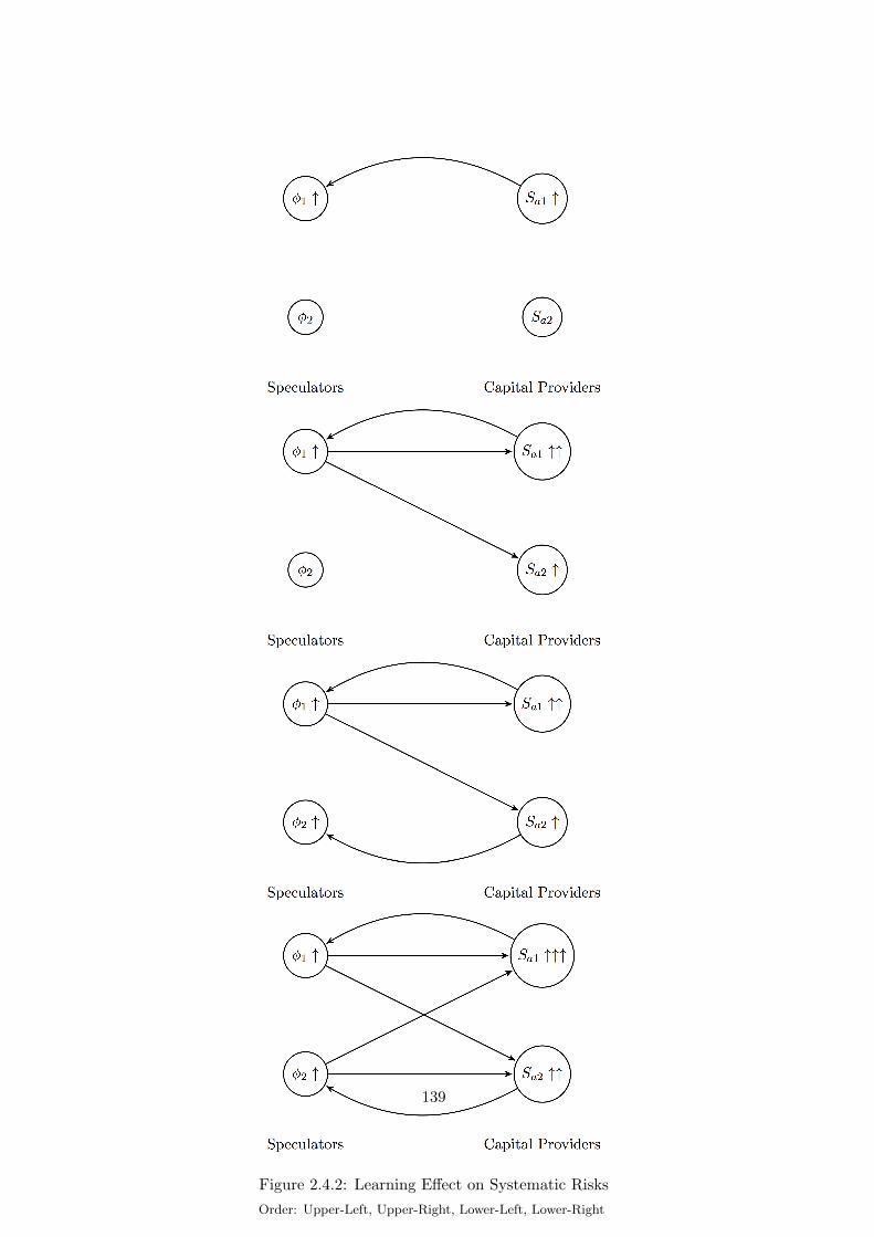
Figure 2.4.2: Learning Effect on Systematic Risks

Order: Upper-Left, Upper-Right, Lower-Left, Lower-Right

139

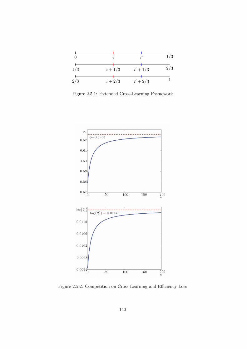
0 1/3

1/3 2/3

2/3 1

i

i+ 1/3

i+ 2/3

i′

i′ + 1/3

i′ + 2/3

Figure 2.5.1: Extended Cross-Learning Framework

Figure 2.5.2: Competition on Cross Learning and Efficiency Loss

140

Bibliography

Aguerrevere, Felipe (2009). “Real Options, Product Market Competition and Asset Returns.”

Journal of Finance, 64: 957983.

Angeletos, George-Marios, Guido Lorenzoni and Alessandro Pavan (2012). “Wall Street

and Silicon Valley: A Delicate Interaction.” Working Paper.

Amador, Manuel and Pierre-Olivier Weill (2010). “Learning from Prices: Public Communica-

tion and Welfare.” Journal of Economic Theory, 147: 910-940.

Barberis, Nicholas, Andrei Shleifer and Robert Vishny (1998). “A Model of Investor Senti-

ment.” Journal of Financial Economics, 49: 307-343.

Bond, Philip, Alex Edmans and Itay Goldstein (2012). “The Real Effects of Financial Markets.”

Annual Review of Finance and Economics, 4: 1-22.

Bhattacharyya, Sugato and Amiyatosh Purnanandam (2011). “Risk-Taking by Banks: What

Did We Know and When Did We Know It?” Working paper.

Brunnermeier, Markus and Stefan Nagel (2004). “Hedge Funds and the Technology Bubble.”

Journal of Finance, 59: 2013-2040.

Brunnermeier, Markus, Thomas Eisenbach and Yuliy Sannikov (2013). “Macroeconomics with

Financial Frictions: A Survey.” in Daron Acemoglu, Manuel Arellano and Eddie Dekel eds., Advances

in Economics and Econometrics, Tenth World Congress of the Econometric Society.

Brunnermeier, Markus and Martin Oehmke (2013). “Bubbles, Financial Crises, and Systemic

Risk.” in George Constantinides, Milton Harris, and Rene Stulz eds., Handbook of the Economics of

Finance, 2B: 1221-1287. North-Holland.

141

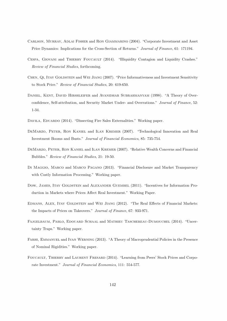
Carlson, Murray, Adlai Fisher and Ron Giammarino (2004). “Corporate Investment and Asset

Price Dynamics: Implications for the Cross-Section of Returns.” Journal of Finance, 61: 171194.

Cespa, Giovani and Thierry Foucault (2014). “Illiquidity Contagion and Liquidity Crashes.”

Review of Financial Studies, forthcoming.

Chen, Qi, Itay Goldstein and Wei Jiang (2007). “Price Informativeness and Investment Sensitivity

to Stock Price.” Review of Financial Studies, 20: 619-650.

Daniel, Kent, David Hirshleifer and Avanidhar Subrahmanyam (1998). “A Theory of Over-

confidence, Self-attribution, and Security Market Under- and Overrations.” Journal of Finance, 52:

1-34.

Davila, Eduardo (2014). “Dissecting Fire Sales Externalities.” Working paper.

DeMarzo, Peter, Ron Kaniel and Ilan Kremer (2007). “Technological Innovation and Real

Investment Booms and Busts.” Journal of Financial Economics, 85: 735-754.

DeMarzo, Peter, Ron Kaniel and Ilan Kremer (2007). “Relative Wealth Concerns and Financial

Bubbles.” Review of Financial Studies, 21: 19-50.

Di Maggio, Marco and Marco Pagano (2013). “Financial Disclosure and Market Transparency

with Costly Information Processing.” Working paper.

Dow, James, Itay Goldstein and Alexander Guembel (2011). “Incentives for Information Pro-

duction in Markets where Prices Affect Real Investment.” Working Paper.

Edmans, Alex, Itay Goldstein and Wei Jiang (2012). “The Real Effects of Financial Markets:

the Impacts of Prices on Takeovers.” Journal of Finance, 67: 933-971.

Fajgelbaum, Pablo, Edouard Schaal and Mathieu Taschereau-Dumouchel (2014). “Uncer-

tainty Traps.” Working paper.

Farhi, Emmanuel and Ivan Werning (2013). “A Theory of Macroprudential Policies in the Presence

of Nominal Rigidities.” Working paper.

Foucault, Thierry and Laurent Fresard (2014). “Learning from Peers’ Stock Prices and Corpo-

rate Investment.” Journal of Financial Economics, 111: 554-577.

142

Froot, Kenneth, David Scharfstein and Jeremy Stein (1992). “Herd on the Street: Informa-

tional Inefficiencies in a Market with Short-Term Speculation.” Journal of Finance, 47: 1461-1484.

Geanakoplos, John and Heracles Polemarchakis (1985). “Existence, Regularity, and Con-

strained Suboptimality of Competitive Allocations When the Asset Market Is Incomplete.” Cowles

Foundation for Research in Economics Discussion Papers 764.

Goldstein, Itay, Emre Ozdenoren and Kathy Yuan (2013). “Trading Frenzies and Their Impact

on Real Investment.” Journal of Financial Economics, 109: 566-582.

Goldstein, Itay and Liyan Yang (2014a). “Market Efficiency and Real Efficiency: The Connect

and Disconnect via Feedback Effects.” Working Paper.

Goldstein, Itay and Liyan Yang (2014b). “Good Disclosure, Bad Disclosure.” Working Paper.

Goldstein, Itay and Liyan Yang (2014c). “Information Diversity and Complementarities in Trading

and Information Acquisition.” Journal of Finance, forthcoming.

Graham, John and Campbell Harvey (2001). “The Theory and Practice of Corporate Finance:

Evidence from the Field.” Journal of Financial Economics, 61: 187-243.

Greenwald, Bruce and Joseph Stiglitz (1986). “Externalities in Economies with Imperfect Infor-

mation and Incomplete Markets.” Quarterly Journal of Economics, 101: 229-264.

Greenwood, Robin and Stefan Nagel (2009). “Inexperienced Investors and Bubbles.” Journal of

Financial Economics, 93: 239-258.

Greenwood, Robin and Samuel Hanson (2013). “Waves in Ship Prices and Investment.” Working

Paper.

He, Zhiguo and Peter Kondor (2013). “Inefficient Investment Waves.” Working Paper.

Hoberg, Gerard and Gordon Phillips (2010). “Real and Financial Industry Booms and Busts.”

Journal of Finance, 65: 45-86.

Hong, Harrison and David Sraer (2013). “Quiet Bubbles.” Journal of Financial Economics, 110:

596-606.

Hong, Harrison and Jeremy Stein (1999). “A Unified Theory of Underraction, Momentum Trading

and Overreaction in Asset Markets.” Journal of Finance, 54: 2143-2184.

143

Johnson, Timothy (2007). “Optimal Learning and New Technology Bubbles.” Journal of Monetary

Economics, 54: 2486-2511.

Jovanovic, Boyan and Glenn McDonald (1994). “The Life Cycle of A Competitive Industry.”

Journal of Political Economy, 102: 322-347.

Kurlat, Pablo and Laura Veldkamp (2013). “Should We Regulate Financial Information?” Work-

ing paper.

Kyle, Albert S. (1985). “Continuous Auctions and Insider Trading.” Econometrica, 53: 1315-1335.

Maksimovic, Vojislav, Gordon Phillips and Liu Yang (2013). “Private and Public Merger

Waves.” Journal of Finance, 68: 2177-2217.

Menzly, Lior and Oguzhan Ozbas (2010). “Market Segmentation and Cross-Predictability of Re-

turns.” Journal of Finance, 65: 1555-1580.

Moskowitz, Tobias and Mark Grinblatt (1999). “Do Industries Explain Momentum?” Journal

of Finance, 54: 1249-1290.

Ozdenoren, Emre and Kathy Yuan (2013). “Endogenous Contractual Externalities.” Working

paper.

Ozoguz, Arzu and Michael Rebello (2013). “Information, Competition, and Investment Sensitivity

to Peer Stock Prices.” Working paper.

Pastor, Lubos and Pietro Veronesi (2006). “Was there a Nasdaq bubble in the late 1990s?”

Journal of Financial Economics, 81: 61-100.

Pastor, Lubos and Pietro Veronesi (2009). “Technological Revolutions and Stock Prices.” Amer-

ican Economic Review, 99: 1451-1483.

Patton, Andrew and Michela Verardo (2012). “Does Beta Move with News? Firm-Specific

Information Flows and Learning about Profitability.” Review of Financial Studies, 25: 2789-2839.

Peng, Lin and Wei Xiong (2006). “Investor Attention, Overconfidence and Category Learning.”

Journal of Financial Economics, 80: 563-602.

Peng, Lin, Wei Xiong and Tim Bollerslev (2007). “Investor Attention and Time-Varying Co-

movements.” European Financial Management, 13: 394-422.

144

Peress, Joel (2010). “Product Market Competition, Insider Trading, and Stock Market Efficiency.”

Journal of Finance, 65: 1-43.

Reinganum, Jennifer (1989). “The Timing of Innovation: Research, Development, and Diffusion.” in

Richard Schmalensee and Robert D. Willig eds., Handbook of Industrial Organization, North Holland,

New York.

Rhodes-Kropf, Matthew, David Robinson and S. Viswanathan (2005). “Valuation Waves and

Merger Activity: the Empirical Evidence.” Journal of Financial Economics, 77: 561-603.

Rhodes-Kropf, Matthew and S. Viswanathan (2004). “Market Valuation and Merger Waves.”

Journal of Finance, 59: 2685-2718.

Scharfstein, David and Jeremy Stein (1990). “Herd Behavior and Investment.” American Eco-

nomic Review, 80: 465-479.

Shleifer, Andrei (1986). “Implementation Cycles.” Journal of Political Economy, 94: 1163-1190.

Sockin, Michael and Wei Xiong (2014a). “Informational Frictions and Commodity Markets.”

Journal of Finance, forthcoming.

Sockin, Michael and Wei Xiong (2014b). “Learning about the Neighborhood: A Model of Housing

Cycles.” Working Paper.

Stiglitz, Joseph (1982). “The Inefficiency of the Stock Market Equilibrium.” Review of Economic

Studies, 49: 241-261.

Subrahmanyam, Avanidhar and Sheridan Titman (2013). “Financial Market Shocks and the

Macroeconomy.” Review of Financial Studies, forthcoming.

Veldkamp, Laura (2006). “Information Markets and the Comovement of Asset Prices.” Review of

Economic Studies, 73: 823-845.

Veldkamp, Laura and Justin Wolfers (2007). “Aggregate Shocks or Aggregate Information?

Costly Information and Business Cycle Comovement.” Journal of Monetary Economics, 54(S): 1-29.

Veldkamp, Laura (2011). Information Choice in Macroeconomics and Finance. Princeton Press.

Vives, Xavier (1993). “How Fast do Rational Agents Learn?” Review of Economic Studies, 60:

329-347.

145

Vives, Xavier (1997). “Learning from Others: A Welfare Analysis.” Games and Economic Behavior,

20: 177-200.

Vives, Xavier (2010). Information and Learning in Markets: The Impact of Market Microstructure.

Princeton Press.

Vives, Xavier (2014). “Endogenous Public Information and Welfare in Market Games.” Working

Paper.

Xiong, Wei (2013). “Bubbles, Crises, and Heterogeneous Beliefs.” in Jean-Pierre Fouque and Joe

Langsam eds., Handbook for Systemic Risk, forthcoming.

146

2.8 Appendix

2.8.1 Proofs

This appendix provides all proofs omitted above with auxiliary results.

Proof of Lemma 2.3.1. According to the equilibrium definition, any speculator (i, j) longs

one share of asset i when φixij + yij > µi and shorts one share otherwise. Equivalently,

speculator (i, j) longs one share of asset i when

φixij + yij√τ−1x φ2i + τ−1y

>µi − (φia+ fi)√τ−1x φ2i + τ−1y

,

and shorts one share otherwise. Thus, in asset market i, all speculators’ aggregate demand is

Di = 1− 2Φ

µi − (φia+ fi)√τ−1x φ2i + τ−1y

.

Hence, in equilibrium, market clearing implies

1− 2Φ

µi − (φia+ fi)√τ−1x φ2i + τ−1y

= 1− 2Φ(ζ + ξi − λ logPi) ,

which further implies that the equilibrium price in asset market i is

Pi = exp

φi

λ√τ−1x φ2i + τ−1y

a+1

λ√τ−1x φ2i + τ−1y

fi +ζ + ξiλ− µi

λ√τ−1x φ2i + τ−1y

.

This concludes the proof.

Proof of Lemma 2.3.2. In a symmetric equilibrium, the capital providers put a same weight

φ on the information of the common shock in any asset market i. Thus, by Lemma 2.3.1, for

147

asset price Pi, its equivalent signal in predicting the common shock a becomes

za(Pi) = a+1

φfi +

√τ−1x φ2 + τ−1y

φ(ζ + ξi) .

Since fi and ξi are both i.i.d. and have zero means, the aggregate price P is equivalent to

the following signal

za(P ) =

∫ 1

0

a+1

φfi +

√τ−1x φ2 + τ−1y

φ(ζ + ξi)

di = a+

√τ−1x φ2 + τ−1y

φζ

in predicting the common shock a. It immediately follows the construction of the other signal

zf,i(P ) in predicting the idiosyncratic shock.

Finally, it is easy to verify that any combination of the asset prices {Pi, i ∈ [0, 1]} cannot

be more informative in predicting the two productivity shocks. This concludes the proof.

Proof of Lemma 2.3.3. From the capital providers’ problem (2.1), the first order condition

is

Ii =κ

cE[exp(a+ fi)|Γi]

=κ

cexp

(E[a+ fi|Γi] +

1

2Var[a+ fi|Γi]

).

By Lemma 2.3.2, we know that sa,i and za(P ) are only informative about the common

shock a and sf,i and zf,i(P ) are only informative about the idiosyncratic shock fi. Applying

Bayesian updating immediately leads to the following optimal investment policy

Ii =κ

cexp

[τsasa,i + τpaza(P )

τa + τsa + τpa+

1

2(τa + τsa + τpa)+τfsf,i + τpfzf,i(P )

τf + τsf + τpf+

1

2(τf + τsf + τpf )

].

This concludes the proof.

Proof of Lemma 2.3.4. This is a direct application of Lemma 2.3.2 to Definition 2.3.2.

148

Proof of Proposition 2.3.1. We proceed step by step.

Step 1: Proof of the existence of the solution.

Following the equilibrium condition (2.10) for the cross-learning case, let

g(φ) = φ− α1 − γ1α2 − γ2

= φ−

τsa+τpaτa+τsa+τpa

+ 1− φ

λ√τ−1x φ2+τ−1

y

τsf+τpfτf+τsf+τpf

+ 1− 1

λ√τ−1x φ2+τ−1

y

τxτa+τxτy

τf+τy

,

where τpa is given by (2.5) and τpf is given by (2.7), both being function of φ. It is easy to

check that limφ→−∞ g(φ) < 0 and limφ→+∞ g(φ) > 0 by the following two equations:

limφ→−∞

τsa+τpaτa+τsa+τpa

+ 1− φ

λ√τ−1x φ2+τ−1

y

τsf+τpfτf+τsf+τpf

+ 1− 1

λ√τ−1x φ2+τ−1

y

τxτa+τxτy

τf+τy

=τx

τa+τxτy

τf+τy

τsa+τζτxτa+τsa+τζτx

+ 1−√τxλ

τsfτf+τsf

+ 1,

and

limφ→+∞

τsa+τpaτa+τsa+τpa

+ 1− φ

λ√τ−1x φ2+τ−1

y

τsf+τpfτf+τsf+τpf

+ 1− 1

λ√τ−1x φ2+τ−1

y

τxτa+τxτy

τf+τy

=τx

τa+τxτy

τf+τy

τsa+τζτxτa+τsa+τζτx

+ 1−√τxλ

τsfτf+τsf

+ 1.

The analysis above indicates that there always exists a solution of φ to the equilibrium

condition (2.10), i.e., g(φ) = 0, by the intermediate value theorem. Especially, when λ >

1/√τ−1x , we know that

f(0) = −τsa+τpa

τa+τsa+τpa+ 1

τsf+τpfτf+τsf+τpf

+ 1− 1

λ√τ−1x

τxτa+τxτy

τf+τy

< 0 .

We conclude that there always exists a positive solution φ > 0 as long as λ is large enough.

Step 2: Proof of the uniqueness of the solution when τf is large enough.

By simple algebra, the equilibrium condition (2.10) is re-expressed as

τsa + τpaτa + τsa + τpa

+ 1− φ

λ√τ−1x φ2 + τ−1

y

τxτa + τx

= φ

τsf + τpfτf + τsf + τpf

+ 1− 1

λ√τ−1x φ2 + τ−1

y

τyτf + τy

.

(2.1)

149

Applying Taylor expansion to the terms in equation (2.1) with respect to τ−1y yields:

τsa + τpaτa + τsa + τpa

= − τaτa + τsa + τpa

− τa(τa + τsa + τpa)2

τζ

τ−2x φ2

τ−1y + o(τ−1

y ) ,

τsf + τpfτf + τsf + τpf

= 1− τfτf + τsf + τpf

− τf(τf + τsf + τpf )2

τξ

τ−2x φ4

τ−1y + o(τ−1

y ) ,

φ

λ√τ−1x φ2 + τ−1

y

=1

λ√τ−1x

− 1

2λτ− 3

2x φ2

τ−1y + o(τ−1

y ) ,

and1

λ√τ−1x φ2 + τ−1

y

=1

λφ√τ−1x

− 1

2λτ− 3

2x φ3

τ−1y + o(τ−1

y ) .

Plugging them back into equation (2.1), we have:

τxτa+τx

τf+τyτy

[2− τa

τa+τsa+τpa− τa

(τa+τsa+τpa)2τζ

τ−2x φ2

τ−1y − 1

λ√τ−1x

+ 1

2λτ− 3

2x φ2

τ−1y + o(τ−1y )

]= φ

[2− τf

τf+τsf+τpf− τf

(τf+τsf+τpf )2

τξτ−2x φ4

τ−1y − 1

λφ√τ−1x

+ 1

2λτ− 3

2x φ3

τ−1y + o(τ−1y )

],

which becomes a cubic equation of φ when τy goes to infinity:

(τsa + τxτζ

τa + τsa + τxτζ+ 1−

√τxλ

)τx

τa + τx=

τsfφ3 + τxτξφ

τfφ2 + τsfφ2 + τxτξ+ φ−

√τxλ

. (2.2)

Note that, the left hand side of equation (2.2) does not depends on φ. Denote by h(φ) the

right hand side of (2.2), and its first order derivative with respect to φ is given by

∂h(φ)

∂φ= 1−

τfφ2

τfφ2 + τsfφ2 + τxτξ+ 1−

2τfτxτξφ2

(τfφ2 + τsfφ2 + τxτξ)2> 0 ,

which indicates that the right hand side of equation (2.2) is increasing in φ and thus we have

a unique solution to equation (2.2). Therefore, since g(φ) is a continuous function of τy, there

always exists one unique solution to g(φ) = 0, i.e., equation (2.1), when τy is large enough.

This concludes the proof.

Proof of Proposition 2.3.2. This proof is similar to the proof of Proposition 2.3.1. In the

150

benchmark case without cross learning, the equilibrium condition (2.11) is re-expressed as

τsa + τpaτa + τsa + τpa

+τpf

τf + τsf + τpfφ′ + 1− φ

λ√τ−1x φ2 + τ−1y

τxτa + τx

= φ

τsf + τpfτf + τsf + τpf

+τpa

τa + τsa + τpa

1

φ′+ 1− 1

λ√τ−1x φ2 + τ−1y

τyτf + τy

,

which further reduces to

(τsa

τa + τsa+ 1−

√τxλ

)τx

τa + τx= φ

(τsf

τf + τsf+ 1−

√τxλφ

), (2.3)

when τy goes to infinity, τξ goes to zero and λ >√τx. Since the right hand side of equation

(2.3) is increasing inf φ, we know that there must exist one unique solution to equation (2.3).

On the other hand, when τξ goes to zero (and when τy goes to infinity and λ >√τx),

equation (2.2) in the case with cross learning becomes

(τsa + τpa

τa + τsa + τpa+ 1−

√τxλ

)τx

τa + τx= φ

(τsf

τf + τsf+ 1−

√τxλφ

). (2.4)

We compare between the two equations (2.3) and (2.4). It is clear that their right hand

sides are the same, while the left hand side of (2.3) (for the benchmark case without cross

learning) is smaller than the left hand side of (2.4) (for the case with cross learning). Thanks

to the continuity with respect to τy and τξ of the two equilibrium conditions (2.11) and (2.10)

in the two cases, we conclude that the equilibrium φ′ in the benchmark case without cross

learning is always lower than the equilibrium φ is the problem with cross learning, as long as

λ >√τx, τy is large enough, and τξ is small enough.

In the following proofs, we will frequently refer to the two notions of investment sensitivity

defined in Definition 2.3.2, i.e., common investment sensitivity Sa and idiosyncratic investment

sensitivity Sf . They are both functions of φ in equilibrium.

151

Proof of Lemma 2.4.1. We first consider the investment beta βI . Recall the investment

policy (2.8), we have

log Ii =τsasa,i + τpaza(P )

τa + τsa + τpa+

1

2(τa + τsa + τpa)+τfsf,i + τpfzf,i(P )

τf + τsf + τpf+

1

2(τf + τsf + τpf ).

Following the definition of βI and after some algebra, we reach

βI =Sa/τa − τsa

(τa+τsa+τpa)2

Sa/τa + Sf/τf.

To simplify the analysis, let g1 = Sa/τa , g2 = τsa/ (τa + τsa + τpa)2 , and g3 = Sf/τf . By

Lemma 2.3.4, it is straightforward that g1 is increasing in φ and both g2 and g3 are decreasing

in φ. Thus, as φ > 0, we also have that g1 is increasing in φ2 and both g2 and g3 are decreasing

in φ2. Furthermore, we have

∂βI∂φ2

=g′1 − g′2g1 + g3

− (g1 − g2)(g′1 + g′3)

(g1 + g3)2

=[(g′1 − g′2)g1 − (g1 − g2)g′1] + (g′1 − g′2)g3 − (g1 − g2)g′3

(g1 + g3)2,

where g′1, g′2 and g′3 stands for the first order derivative with respect to φ2.

Since we know that g′1−g′2 > g′1 (due to the fact that g2 is decreasing in φ2) and g1 > g1−g2,

we have (g′1 − g′2)g1 − (g1 − g2)g′1 > 0. Meanwhile, we have g′1 > 0, g′2 < 0, and g3 > 0, so that

(g′1−g′2)g3 > 0. Lastly, since g1 > g2 and g′3 < 0, we also know that (g1−g2)g′3 < 0. Therefore,

we conclude that ∂βI/∂φ2 > 0, i.e., βI is an increasing function of φ when φ > 0.

We then consider the price beta βP . Recall the pricing function (2.1), we have

logPi =φ

λ√τ−1x φ2 + τ−1y

a+1

λ√τ−1x φ2 + τ−1y

fi +ζ + ξiλ− µ

λ√τ−1x φ2 + τ−1y

.

152

Following the definition of βP and after some algebra, we reach that

βP =

φ2

τ−1x φ2+τ−1

y

1τa

+ 1τζ

φ2

τ−1x φ2+τ−1

y

1τa

+ 1τζ

+ 1τ−1x φ2+τ−1

y

1τf

+ 1τξ

.

To simplify, let

h1 =φ2

τ−1x φ2 + τ−1y

1

τa+

1

τζ(2.5)

and

h2 =1

τ−1x φ2 + τ−1y

1

τf+

1

τξ. (2.6)

It is straightforward that h1 is increasing in φ and h2 is decreasing in φ. Hence, we have

∂βP∂φ2

=−g1 ∂g2∂φ2

(g1 + g2)2> 0 ,

which indicates that βP is an increasing function of φ when φ > 0.

Proof of Lemma 2.4.2. We first consider common investment correlation βA. Recall the

investment policy (2.8) and the definition of βA, we have

βA =Cov(log Ii, logA)√

Var(log Ii)√

Var(logA)

=

τsa+τpaτa+τsa+τpa

√τa

√τsa+τpa

τa+τsa+τpa1τa

+τf+τpf

τf+τsf+τpf

1τf

=Sa√

τa√Sa/τa + Sf/τf

.

It is convenient for us to consider instead

1

τaβ2A=Sa/τa + Sf/τf

S2a

=1

τaSa+

SfτfS2

a

.

By Lemma 2.3.4, since Sa is increasing in φ2 and Sf is decreasing in φ2 when φ > 0, it

is straightforward that 1/τaβ2A is decreasing in φ2. This indicates that βA is an increasing

function of φ when φ > 0.

153

We then consider the idiosyncratic investment correlation βF . Again, recall the investment

policy (2.8) and the definition of βF , we have

βF =Cov(log Ii, logFi)√

Var(log Ii)√

Var(logFi)

=

τf+τpfτf+τsf+τpf

√τf

√τsa+τpa

τa+τsa+τpa1τa

+τf+τpf

τf+τsf+τpf

1τf

=Sf

√τf√Sa/τa + Sf/τf

.

Similarly, it is convenient for us to consider instead

1

τfβ2F

=Sa/τa + Sf/τf

S2f

=SaτaS2

f

+1

τfSf,

which is decreasing in φ2, again by Lemma 2.3.4. Hence, we conclude that βF is an increasing

function of φ as well, when φ > 0.

Proof of Lemma 2.4.3. Following Assumption 2.4.1, we keep the ratios τsa/τa and τx/τa

constant when consider the changes of τa. We also focus on the case when τy and λ are large

enough so that a unique solution of φ is guaranteed. Specifically, the reduced equilibrium

condition (2.2) (in the proof of Proposition 2.3.1) is re-expressed as

τsa/τa + τxτζ/τaτa(1 + τsa/τa + τxτζ/τa)

τx/τa1 + τx/τa

+τx/τa

1 + τx/τa+

√τxτaτa

λ

1

1 + τx/τa=

τsfφ3 + τx

τaτξφτa

τfφ2 + τsfφ2 + τxτaτξτa

+φ .

(2.7)

When λ is high enough, the first order derivative of the left hand side of equation (2.7)

with respect to τa is

−τsa/τa + τxτζ/τa

τ2a (1 + τsa/τa + τxτζ/τa)

τx/τa1 + τx/τa

+

√τx/τaλ

1

1 + τx/τa

1

2√τa< 0 .

And it is straightforward that the right hand side of (2.7) is an increasing function of τa. Thus,

when τa increases, the left hand side of (2.7) decreases, which further calls for a decreasing φ

to make the right hand side of (2.7) to decrease as well. This concludes the proof.

154

Proof of Proposition 2.4.1. Again, following Assumption 2.4.1, we keep the ratios τsa/τa

and τx/τa constant when consider the changes of τa. We still focus on the case when τy and λ

are large enough so that a unique solution of φ is guaranteed.

We first consider the investment beta

βI =Sa − g

Sa + τaSf/τf,

where

g =

(τsa

τa + τsa + τpa

)2 τaτsa

. (2.8)

It is instructive for us to decompose the total effects of the changing of τa on βI into two

parts: the mechanical effect and the cross-learning effect:

dβI(τa, φ)

dτa=∂βI(τa, φ)

∂τa+∂βI(τa, φ)

∂φ

∂φ

∂τa.

The sign of the second term, the cross-learning effect, is straightforward by Lemma 2.4.1

and Lemma 2.4.3. Specifically, Lemma 2.4.1 indicates that ∂βI(τa, φ)/∂φ > 0 and Lemma

2.4.3 indicates that ∂φ/∂τa < 0, so that the cross-learning effect is negative in this case.

For the first term, the mechanical effect, since we keep τsa/τa and τx/τa constant and

τpa = τxτς when τy goes to infinity, we know that Sa and g are constant in this case. On the

other hand, Sf is increasing in τx given τpf = τxτξ/φ2 and thus is also increasing in τa given

that τx/τa is constant. This indicates that τaSf/τf is increasing in τa. Hence, we know that

∂βI(τa, φ)/∂τa < 0, i.e., the mechanical effect is negative as well.

Taking the two effects together, we know that the total effect is also negative, i.e., dβI(τa, φ)/dτa <

0.

We then consider the price beta

βP =

φ2

τ−1x φ2+τ−1

y

1τa

+ 1τζ

φ2

τ−1x φ2+τ−1

y

1τa

+ 1τζ

+ 1τ−1x φ2+τ−1

y

1τf

+ 1τξ

=h1

h1 + h2,

155

where h1 and h2 are already defined in (2.5) and (2.6) (in the proof of Lemma 2.4.1).

Again, we decompose the total effects of the changing of τa on βP into two parts: the

mechanical effect and the cross-learning effect:

dβP (τa, φ)

dτa=∂βP (τa, φ)

∂τa+∂βP (τa, φ)

∂φ

∂φ

∂τa.

Keep in mind that we keep τsa/τa and τx/τa constant in this case. First, it is straightfor-

ward to see that the mechanical effect ∂βP (τa, φ)/∂τa is negative, because βP is an increasing

function of h1 that is in turn decreasing in τa at the same time. Furthermore, Lemma 2.4.1

indicates that ∂βP (τa, φ)/∂φ > 0 and Lemma 2.4.3 indicates that ∂φ/∂τa < 0, which together

imply that the cross-learning effect is negative as well. Therefore, we conclude that the total

effect is also negative, i.e., dβP (τa, φ)/dτa < 0.

Proof of Lemma 2.4.4. The proof is similar to the proof of Lemma 2.4.3. We again focus

on the case when τy and λ are large enough so that a unique solution of φ is guaranteed. In

this case, we recall the reduced equilibrium condition (2.2) (in the proof of Proposition 2.3.1):

(τsa + τxτζ

τa + τsa + τxτζ+ 1−

√τxλ

)τx

τa + τx=

τsfφ3 + τxτξφ

τfφ2 + τsfφ2 + τxτξ+ φ−

√τxλ

.

It is clear that the left hand side of (2.2) is increasing in τsa. Hence, when τsa increase, the

right hand side of (2.2) increases as well. On the other hand, we have already known that the

right hand side of (2.2) is increasing in φ. Hence, in equilibrium, φ increases. This indicates

that φ is an increasing function of τsa.

The analysis is similar for τsf . The right hand side of (2.2) is increasing in τsf , while the

left hand side is independent of τsf . Thus, when τsf increase, φ decreases to ensure a constant

right hand side of (2.2). This indicates that φ is a decreasing function of τsf .

Proof of Proposition 2.4.2. We first consider the comparative statics with respect to τsa.

156

For the investment beta βI , we have

βI = 1−Sf/τf + g/τaSa/τa + Sf/τf

,

where g is already defined in (2.8) (in the proof of Proposition 2.4.1).

We also decompose the total effects of the changing of τsa on βI into two parts: the

mechanical effect and the cross-learning effect:

dβI(τsa, φ)

dτsa=∂βI(τsa, φ)

∂τsa+∂βI(τsa, φ)

∂φ

∂φ

∂τsa.

Clearly, Lemma 2.4.1 and Lemma 2.4.4 indicate that the second term, the cross-learning

effect, is positive. For the first term, the mechanical effect, we first know that Sa is increasing

in τsa, given φ fixed. Also, it is easy to show that g/τa is increasing in τsa (given φ fixed)

when τsa < τa + τxτζ , and decreasing in τsa (also given φ fixed) when τsa > τa + τxτζ . Hence,

we conclude that when τsa > τa + τxτζ , the mechanical effect is positive, and thus total effect

dβI(τsa, φ)/dτsa is positive as well. When τsa < τa + τxτζ , the mechanical effect is negative

and thus the total effect is ambiguous.

For the price beta βP , there is only cross-learning effect but no mechanical effect. Hence,

by Lemma 2.4.1 and Lemma 2.4.4 we have that

dβP (τsa, φ)

dτsa=∂βP (τsa, φ)

∂φ

∂φ

∂τsa> 0 .

We then consider the comparative statics with respect to τsf in a similar manner. For the

investment beta βI , we have

βI =Sa/τa − g/τaSa/τa + Sf/τf

.

By the similar decomposition and again by Lemma 2.4.1 and Lemma 2.4.4, we know that

both the mechanical effect and the cross-learning effect in this case are negative. So that the

157

total effect is also negative:

dβI(τsf , φ)

dτsf=∂βI(τsf , φ)

∂τsf+∂βI(τsf , φ)

∂φ

∂φ

∂τsf< 0 .

For the price βP , again, there is only cross-learning effect but no mechanical effect. Hence,

by Lemma 2.4.1 and Lemma 2.4.4 we have that

dβP (τsf , φ)

dτsf=∂βP (τsf , φ)

∂φ

∂φ

∂τsf< 0 .

This concludes the proof.

Proof of Lemma 2.4.5. We focus on the case when τy and λ are large enough so that a

unique solution of φ is guaranteed. We first consider the effect of λ. Recall the re-expressed

reduced equilibrium condition (2.7) (in the proof of Lemma 2.4.3):

τsa/τa + τxτζ/τaτa(1 + τsa/τa + τxτζ/τa)

τx/τa1 + τx/τa

+τx/τa

1 + τx/τa+

√τxτaτa

λ

1

1 + τx/τa=

τsfφ3 + τx

τaτξφτa

τfφ2 + τsfφ2 + τxτaτξτa

+φ .

It is clear that the left hand side of (2.7) is decreasing in λ while the right hand side is

independent of λ. Hence, when λ increases, φ decreases in equilibrium.

We then consider the effects of τζ and τξ. Recall the reduced equilibrium condition (2.2)

(in the proof of Proposition 2.3.1):

(τsa + τxτζ

τa + τsa + τxτζ+ 1−

√τxλ

)τx

τa + τx=

τsfφ3 + τxτξφ

τfφ2 + τsfφ2 + τxτξ+ φ−

√τxλ

.

On the one hand, the left hand side of (2.2) is increasing in τζ , while the right hand side

is independent of τζ , so that φ is increasing in τζ in equilibrium. On the other hand, the right

hand side of (2.2) is increasing in τξ while the left hand side is independent of τξ, so that φ is

decreasing in τξ in equilibrium.

158

Proof of Proposition 2.4.3. We first consider the comparative statics with respect to λ.

Since λ has no mechanical effect on ether βI or βP , we focus on the cross-learning effect along.

By Lemma 2.4.1 and Lemma 2.4.5, we know that both βP and βI are decreasing in λ.

We then consider the comparative statics with respect to τζ . For the investment beta βI ,

we have

βI =Sa − g

Sa + τaSf/τf,

where g is defined in (2.8) (in the proof of Proposition 2.4.1).

Again, we decompose the total effects of the changing of τζ on βI into two parts: the

mechanical effect and the cross-learning effect:

dβI(τζ , φ)

dτζ=∂βI(τζ , φ)

∂τζ+∂βI(τζ , φ)

∂φ

∂φ

∂τζ.

By Lemma 2.4.1 and Lemma 2.4.5, we know that the cross-learning effect is positive. For

the mechanical effect, when φ is fixed, it is easy to show that ∂βI(τζ , φ)/∂τpa > 0. Since we

know that ∂τpa/∂τζ > 0, we get that the mechanical effect is also positive. Hence, the total

effect dβI(τζ , φ)/dτζ is positive.

However, the total effect on the price beta βP is ambiguous in this case. We have

βP =h1

h1 + h2,

where h1 and h2 are already defined in (2.5) and (2.6) (in the proof of Lemma 2.4.1). Decom-

position gives

dβP (τζ , φ)

dτζ=∂βP (τζ , φ)

∂τζ+∂βP (τζ , φ)

∂φ

∂φ

∂τζ.

Lemma 2.4.1 and Lemma 2.4.5 give a positive cross-learning effect, i.e., the second term.

However, it is easy to show that the first term, the mechanical effect, is negative. Hence, the

total effect is ambiguous and will be determined by other model parameters.

We finally consider the comparative statics with respect to τξ. Similarly, we follow the

159

decomposition above. For the investment beta βI , by Lemma 2.4.1 and Lemma 2.4.5, we know

that the cross-learning effect is negative. For the mechanical effect, when φ is fixed, it is easy to

show that ∂βI(τξ, φ)/∂τpf > 0. Since we know that ∂τpf/∂τξ > 0, we get that the mechanical

effect is also negative. Hence, the total effect dβI(τξ, φ)/dτξ is negative. Following similar

arguments and again by Lemma 2.4.1 and Lemma 2.4.5, we know that both the mechanical

effect and the cross-learning effect on the price beta βP are also negative, so that the total

effect on βP is negative as well.

Proof of Proposition 2.5.1. Following the definition of real investment efficiency, we know

that

R =

∫ 1

0Ridi ,

where

Ri = E[AFiIi −

c

2I2i

]=κ(2− κ)

2cE [AFiE [AFi|Γi]] ,

and

E[AFi|Γi] = exp

[τsasa,i + τpaza(P )

τa + τsa + τpa+

1

2(τa + τsa + τpa)+τfsf,i + τpfzf,i(P )

τf + τsf + τpf+

1

2(τf + τsf + τpf )

].

Since κ and c are constant, without loss of generality, we set κ = 1 and c = 0.5 to ease the

exposition. After some tedious algebra, the investment efficiency R is re-expressed in a much

simpler and more intuitive form:

R = exp

(1 + Saτa

+1 + Sfτf

). (2.9)

We solve for the socially optimal φ∗ that maximizes R. Taking the first order condition

gives

∂ logR

∂(φ2)=

τ2xτζτy(τa + τsa + τpa)2

1

(τx + τyφ2)2−

τxτ2y τξ

(τf + τsf + τpf )21

(τx + τyφ2)2= 0 , (2.10)

160

which reduces to

(τa + τsa + τpa)2

(τf + τsf + τpf )2=τxτζτyτξ

. (2.11)

Since τpa is increasing in φ2 while τpf is decreasing in φ2, we know that the left hand side

of (2.11) is increasing in φ2. Therefore, there is a unique non-negative solution of φ∗.

We further compare between the socially optimal weight φ∗ and the weight φ in the cross-

learning equilibrium, focusing on the case in which τy and λ are large enough so that there is

always a unique positive solution of φ. We re-express the first order condition (2.10) as

∂ logR

∂(φ2)=

τxτ2y

(τa + τsa + τpa)2

[τxτζτy−

(τa + τsa + τpa)2τξ

(τf + τsf + τpf )2

]= 0 . (2.12)

When τy goes to infinity, we know that τxτζ/τy goes to 0, and we also have

(τa + τsa + τpaτf + τsf + τpf

)2

=

(τa + τsa + τxτζ

τf + τsf + τxτζ/φ2

)2

> 0 .

Hence, when τy and λ are large enough, the left hand side of (2.12) is always negative. There-

fore, we conclude that the cross-learning equilibrium φ is always larger than the socially optimal

φ∗ when τy and λ are large enough.

Proof of Proposition 2.5.2. Recall the expression of investment efficiency (2.9):

R = exp

(1 + Saτa

+1 + Sfτf

).

We again focus on the case when τy and λ are large enough so that a unique solution of φ is

guaranteed. We first consider the comparative statics with respect to λ. Lemma 2.3.4 implies

that ∂Sf/∂φ < 0 and Lemma 2.4.5 implies that ∂φ/∂λ < 0. Since there is no direct effect of λ

on Sf , we know that Sf is increasing in λ in equilibrium. Moreover, because the effect of φ on

Sa is negligible when τy is sufficiently large, we eventually know that that R is an increasing

function of λ.

161

We then consider τξ. Similarly, Lemma 2.3.4 implies that ∂Sf/∂φ < 0 and Lemma 2.4.5

implies that ∂φ/∂τξ < 0, so that Sf , and thus R is increasing in τξ in equilibrium.

We finally consider τsf . It is clear that ∂Sf/∂τsf > 0, i.e., the mechanical effect is positive.

For the cross-learning effect, Lemma 2.3.4 implies that ∂Sf/∂φ < 0 and Lemma 2.4.4 implies

that ∂φ/∂τξ < 0. Hence, the total effect is positive as well, i.e., Sf is increasing in τsf in

equilibrium. Since the effect of φ on Sa is negligible when τy is sufficiently large, we eventually

know that that R is an increasing function of τsf .

Proof of Proposition 2.5.3. Part i) is straightforward following the proofs of Proposition

2.3.1 and Proposition 2.3.2. For part ii), we make use of the conditional expectation (2.12).

Specifically, we have

Var(z) =

σ11 σ12 σ13 σ14

σ21 σ22 σ23 σ24

σ31 σ32 σ33 σ34

σ41 σ42 σ43 σ44

,

where

σ11 = τ−1a + τ−1sa ,

σ12 = 0 ,

σ13 = φnτ−1a ,

σ14 = φnτ−1a ,

σ22 = τ−1f + τ−1sf ,

σ23 = τ−1f ,

σ24 = 0 ,

σ33 = τ−1f + φ2nτ−1a + (τ−1x φ2n + τ−1y )(τ−1ζ + τ−1ξ ) ,

σ34 = φ2nτ−1a + (τ−1x φ2n + τ−1y )τ−1ζ ,

162

σ44 =τ−1fn− 1

+ φ2nτ−1a + (τ−1x φ2n + τ−1y )

(τ−1ζ +

τ−1ξn− 1

),

and

Cov(z, a+ fi) = [τ−1a , τ−1f , φnτ−1a + τ−1f , φnτ

−1a ] .

By condition (2.12), we get the expressions of San and Sfn after some tedious algebra

and plug them into the equilibrium condition. Denote by RHS the right hand side of the

equilibrium condition (2.13) and we get

∂ limτy→∞RHS(φn, n)

∂n= C1C2C3C4C5(C6 + C7 + C8)

2 , (2.13)

where

C1 = φ2n(τf + τsf )τζ + τxτζτξ − φn(τa + τsa + τxτζ)τξ ,

C2 = φ2nτa(τf + 2τsf )τζ + 2τaτxτζτξ + φnτf (τa + 2(τsa + τxτζ))τξ ,

C3 = φ2nτf + τxτξ ,

C4 = φ2nτfτ2xτξ ,

C5 = τa + τx ,

C6 = φ3nτ2f τxτζτξ + φnτfτ

2xτζτ

2ξ + 2(τa + τsa)τ

2xτζτ

2ξ ,

C7 = φ4nτf (τf + 2τsf )((τa + τsa)τζ + n(τa + τsa + τxτζ)τξ) ,

C8 = φ2nτxτξ((τa + τsa)(3τf + 2τsf )τζ + ((2n− 1)τf + 2τsf )(τa + τsa + τxτζ)τξ) .

Note that, only the first term C1 has a negative component. However, when τξ is small

enough, C1 is always strictly positive, so is the entire derivative (2.13). It implies that when τy

is large enough and τξ is small enough, the equilibrium φn is increasing in n. Also, the proof

of Proposition 2.5.1 directly implies that φ′(= φ1) > φ∗, so that φn > φ∗ for all n > 1.

Finally, for part iii), by the proof of Proposition 2.5.1, in particular condition (2.9), we

163

know that

Rn = exp

(1 + Sa(φn)

τa+

1 + Sf (φn)

τf

),

where Sa and Sf are the capital providers’ investment sensitivities in the baseline cross-learning

case pinned down by however the equilibrium weight in the corresponding n-learning equilib-

rium. By Lemma 2.3.4, it follows that R < Rn < R∗ for all n > 1. This concludes the

proof.

164

Chapter 3

How Options Affect Information

Acquisition and Asset Pricing

Shiyang Huang

Abstract: We study the effect of introducing an options market on investors’ incentive

to collect private information in a rational expectation equilibrium model. We show that an

options market has two effects on information acquisition: a negative effect, as options act

as substitutes for information, and a positive effect, as informed investors have less need for

options and can earn profits from selling them. When the population of informed investors

is high because of the low information acquisition cost, the supply for options is larger than

the demand, leading to low option prices. Low option prices in turn induce investors to use

options instead of information to reduce risk, while informed investors have little opportunity

to earn profits from selling options to cover their information acquisition cost. Introducing

an options market thus decreases investors’ incentive to acquire information, and the prices of

the underlying assets become less informative, leading to lower prices and higher volatilities.

A dynamic extension of this analysis shows that introducing an options market increases the

price reactions to earnings announcements. However, when the information acquisition cost

is high, the opposite effects arise. Further analysis shows that our results are robust for

165

more general derivatives. These results provide a potentially unified theory to reconcile the

conflicting empirical findings on the options listing of individual stocks in both the U.S. market

and international markets.

166

3.1 Introduction

As one of the largest derivative markets, the options market has experienced tremendous

growth (see Figure 3.1).1 Further, the effect of options listing on the underlying asset market

is a hot topic in policy, industry and academia, and it has become extremely important since

the financial crisis of 2007-08.2 Although many empirical studies address this issue, findings

regarding options listing around the world are conflicting. As one example, in the U.S. mar-

ket, the effects of options listing on the underlying individual stocks over the last 30 years

are completely different from such effects 30 years ago.3 Indeed, for the period before 1980,

previous empirical studies find that options listing increased underlying stock prices, decreased

volatilities, and decreased price reactions to earnings announcements (Conrad, 1999, Detemple

and Jorion, 1990 and Skinner, 1989). However, for the period after 1980, recent studies find

the opposite effects (Sorescu, 2000 and Mayhew and Mihov, 2000). There are no plausible

explanations for these conflicting findings. Hence, they remain puzzling.

To our knowledge, few theoretical studies examine the effects of derivatives on their under-

lying assets with endogenous information acquisition. Among the few studies, Cao (1999) and

Massa (2002) show that introducing derivatives, including options, increases the underlying as-

set’s price, decreases volatility and decreases price reactions to earnings announcements. They

thus provide explanations to the empirical findings regarding options listing in U.S. before

1980, but offer little guidance on the effects after 1980.

In this paper, we exam the effect of an options market on investors’ incentive to collect

private information in a rational expectation equilibrium model. Following the canonical frame-

works of Grossman and Stiglitz (1980) and Hellwig (1980), we have one risky asset and one

1Data Source: SELECT SEC AND MARKET DATA FISCAL 2013. Data is about all sales of options listedon exchange and excludes options on indexes

2After credit crunch of 2007-08, The Dodd-Frank Wall Street Reform and Consumer Protection Act , whichwas signed into federal law on July 21, 2010, is considered to bring most significant changes to financial regulationon derivative markets including interest rate option and currency option. Then there is a hot debate on whetherDodd-Frank is enough to prevent systemic risk.

3Although most empirical studies are about U.S. market, there are some evidences to show that option listingdecreases price and increases volatility of underlying individual stocks in developed markets, such as Germany(Heer et al., 1997), while it increases price and decreases volatility in developing markets, such as India (Nair,2008).

167

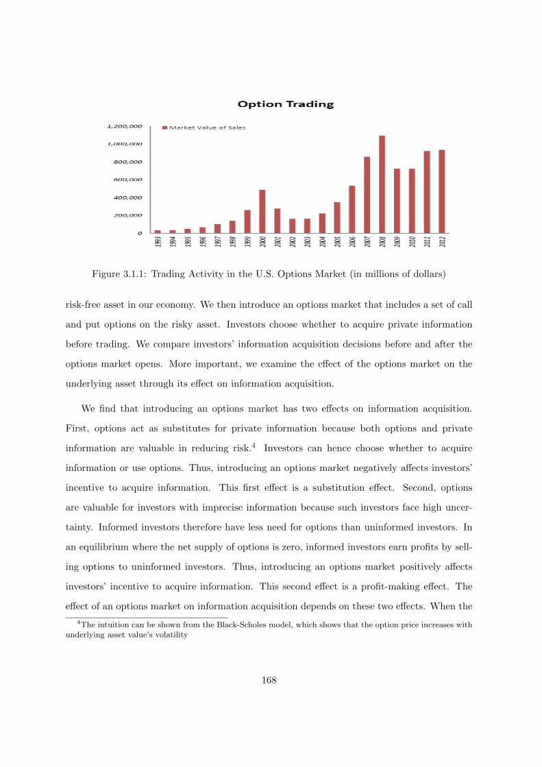
Figure 3.1.1: Trading Activity in the U.S. Options Market (in millions of dollars)

risk-free asset in our economy. We then introduce an options market that includes a set of call

and put options on the risky asset. Investors choose whether to acquire private information

before trading. We compare investors’ information acquisition decisions before and after the

options market opens. More important, we examine the effect of the options market on the

underlying asset through its effect on information acquisition.

We find that introducing an options market has two effects on information acquisition.

First, options act as substitutes for private information because both options and private

information are valuable in reducing risk.4 Investors can hence choose whether to acquire

information or use options. Thus, introducing an options market negatively affects investors’

incentive to acquire information. This first effect is a substitution effect. Second, options

are valuable for investors with imprecise information because such investors face high uncer-

tainty. Informed investors therefore have less need for options than uninformed investors. In

an equilibrium where the net supply of options is zero, informed investors earn profits by sell-

ing options to uninformed investors. Thus, introducing an options market positively affects

investors’ incentive to acquire information. This second effect is a profit-making effect. The

effect of an options market on information acquisition depends on these two effects. When the

4The intuition can be shown from the Black-Scholes model, which shows that the option price increases withunderlying asset value’s volatility

168

information acquisition cost is low, the population of informed investors is high, which leads to

a lower demand than supply for options. Consequently, the option prices are low, affording in-

formed investors little opportunity to cover the information acquisition cost by selling options.

Meanwhile, investors can use cheap options instead of private information to reduce their risk.

Therefore, the two effects work in conjunction to decrease investors’ incentive to acquire infor-

mation. The price of the underlying asset then becomes less informative, resulting in a lower

price and higher volatility. With less precise private information, investors must rely more on

public information, which generates greater price reactions to earnings announcements. By

contrast, when the information acquisition cost is sufficiently high, the population of informed

investors is low, which leads to a higher demand than supply for options. Consequently, option

prices are high, offering informed investors large opportunity to cover the information acqui-

sition cost by selling options. Therefore, the profit-making effect exerts a larger counteracting

force against the substitution effect, leading to opposite effects on information acquisition and

asset pricing. Moreover, we show that our mechanism is robust for other derivatives, such as

straddles.

We also find that the effect of an options market on information acquisition depends on the

precision of public information. When public information is precise, the population of informed

investors is low before the options market opens. Consequently, the demand for options is

larger than the supply, affording informed investors large opportunity to earn profits. Thus,

introducing an options market increases investors’ incentive to collect private information,

increases the price of the underlying asset, decreases volatility, and decreases price reactions

to earnings announcements. When public information is imprecise, the population of informed

investors is high, leading to low option prices. Consequently, the opposite effects on the

underlying asset arise.

Moreover, we show that the introduction of additional trading rounds has similar effects

to the introduction of an options market. Brennan and Cao (1996) argues that additional

trading rounds, which can be interpreted as after-hour or round-the-clock trading, can improve

the welfare of all investors because both additional trading rounds and derivatives markets

169

increase risk-sharing opportunities. However, their effect on information acquisition is unclear.

Following Brennan and Cao (1996), we extend our model to consider multiple rounds of trading,

where each round provides a new public information. Complementing to their study, we find

that additional trading rounds produce asymmetric benefits for different groups, which leads

to non-monotonic effects on information acquisition. Because risk sharing occurs between

different groups, the relative benefits depend on the competition within each group. For

example, when the population of informed investors is high, the competition within the group

of informed investors is high. Consequently, the benefit from more risk-sharing opportunities

is lower for informed investors than for uninformed investors, which reduces the marginal

benefit of information. Thus, when the population of informed investors is high because of

the low information acquisition cost, introducing additional trading rounds decreases investors’

incentive to acquire information, lowering the asset price and increasing volatility. When the

information acquisition cost is high, the opposite effects arise.

Our results indicate that the effects of options listing on the underlying assets depend on

the information acquisition cost. Our results therefore provide a unified explanation for the

conflicting findings regarding the effects of options listing on underlying individual stocks in

the U.S. market and international markets. For example, before 1980 when information ac-

quisition cost is conventionally believed to have been high, our results are consistent with the

findings in U.S. that options listing increased underlying stock prices (Branch and Finnerty,

1981, Conrad, 1999 and Detemple and Jorion, 1990), decreased volatilities (Hayes and Tennen-

haum, 1979, Skinner, 1989, Conrad, 1999, Ho, 1993 and Damodaran, 1991), and decreased price

reactions to earnings announcements (Jennings and Starks, 1986, Skinner, 1990, Damodaran,

1991 and Ho, 1993 ).5 After 1980 when information acquisition cost is conventionally believed

to be low, our results are consistent with the opposite empirical findings that options listings

decrease underlying stock prices (Detemple and Jorion, 1990, Sorescu, 2000 and Mayhew and

Mihov, 2000), increase volatilities(Freund et al., 1994, Bollen, 1998 and Mayhew and Mihov,

2000), and increase price reactions to earnings announcements (Mendenhall and Fehrs, 1999).

5Information acquisition cost is lower after 1980 than that before 1980 because the technology is developedand it is easier for investors to search for information.

170

Meanwhile, our results could also explain the empirical findings in international markets. For

example, according to the conventional belief, the information acquisition cost is high in emerg-

ing markets, but low in developed markets. Our results are consistent with existing empirical

findings: options listings increase the underlying stock prices and decrease volatilities in emerg-

ing markets, such as India (Nair, 2008), but decrease the underlying stock prices and increase

volatilities in some developed markets, such as Germany (Heer et al., 1997).

Related Literature Our study is related to several strands of literature. First, this study

is associated with theoretical studies on the effects of derivatives on underlying assets, such

as those by Grossman (1988), Biais and Hillion (1994), Huang and Wang (1997), Cao (1999)

and Massa (2002). Cao (1999) and Massa (2002) are the most relevant to the present study,

as they examine the effects of derivatives on information acquisition. Both authors find that

introducing derivatives increases the prices of underlying assets, decreases price volatilities and

decreases the price reactions to earnings announcements. The derivative examined in Massa

(2002) conveys new information, which leads to increased price informativeness. By contrast,

the derivatives examined in Cao (1999) and our study do not convey any additional informa-

tion by themselves. However, Cao (1999) finds only a profit-making effect for the examined

derivatives. Specifically, the author considers two groups of investors: inactive investors, who

are unable to acquire information, and active investors, who determine the precision of pri-

vate information. The author concludes that introducing derivatives increases the information

precisions for active investors. However, in his model, the inactive investors are not able to

acquire information, which hinders the substitution effect. Thus, derivatives have monotonic

effects on information acquisition. In contrast to Cao (1999) and Massa (2002), we find that

derivatives have two effects on information acquisitions: substitution effect and profit-making

effect. More important, we find that the effects of derivatives on information acquisition and

the underlying asset depend on the information acquisition cost and the precision of public

information.

Meanwhile, our approach takes a first step to model an explicit options market in an

economy with information asymmetry. AlthoughCao (1999) studies the effects of derivatives

171

on their underlying assets, the derivatives in the proposed model take reduced forms and they

are interpreted as straddles. The most relevant paper to ours is by Cao and Ou-Yang (2009),

who also model a set of call and put options. However, the authors only conduct the analysis

in an economy with heterogeneous beliefs without any implications for information acquisition.

Our work is also related to the large strand of literature on financial innovation (Allen

and Gale, 1994, Brock, Hommes and Wagener, 2009, Dow, 1998, Dieckmann, 2011, Duffie and

Rohi, 1995, Simsek, 2013a,b, Weyl, 2007 and Chabakauri, Yuan, Zachariadis, 2014). However,

most studies in this literature stream examine the impact of financial innovations without

information asymmetry. For example, Brock, Hommes and Wagener (2009), Simsek (2013a)

and Simsek (2013b) emphasize the destabilizing effect of financial innovations due to hetero-

geneous beliefs. The most relevant paper to ours in this body of literature is by Dow (1998),

who proposes a hedge-more/bet-more effect in an economy with asymmetric information. The

author finds that a new asset induces risk averse arbitrageurs to hedge their positions in the

preexisting security, which affects the old market’s liquidity. This hedge-more/bet-more effect

may have a negative effect on all investors’ welfare. However, we show that options do not

have a direct effect on the underlying asset, which confirms the findings by Chabakauri, Yuan,

Zachariadis (2014). Moreover, we find that options affect the underlying assets through their

effects on information acquisition.

The reminder of the paper is organized as follows. We introduce the model setup in Section

2 and solve a model without an options market. In Section 3, we study the effects of an options

market on information acquisition and the underlying asset in a static model. Section 4 then

extends the static model to a dynamic model. Section 5 discusses more general derivative.

Section 6 concludes and discusses our empirical predictions.

3.2 Model

Based on the canonical frameworks with one risky asset and one risk-free asset by Grossman

and Stiglitz (1980) and Hellwig (1980), we introduce an options market. Our goal is to compare

172

the equilibrium population of informed investors and asset pricing before and after an options

market is introduced into the economy. Before we solve the equilibrium in the economy with

the options market, we solve the equilibrium in the economy without the options market in

this section.

3.2.1 Timeline and assets

There are two periods in our economy, T = 0, 1. There is one risk-free asset and one risky asset.

The risk-free asset is in zero supply, and it pays off one unit of a consumption good without

uncertainty. The risky asset pays off D and has a positive supply of X, where D ∼ N(D, 1h).

There is an options market in our economy, and the underlying asset is the risky asset.

Following Cao and Ou-Yang (2009), we assume that the options market consists of a set of call

and put options. The strike price of one specific option is denoted by G. The call option with

strike price G then has a payoff as (D−G)+, whereas the put option with strike price G has a

payoff as (G−D)+ . The net supply of each option is zero. Because of the put-call parity, we

can only consider call options with positive strike prices and put options with negative strike

prices to simplify our analysis.6 We assume that informed investor i’s demand for risky asset

is Xi, that his demand for call options with strike prices G to G + dG is Xi,CG, and that his

demand for put options with strike prices G to G+dG is Xi,PG. Moreover, we assume that the

uninformed investors’ demand for risky asset is XU , that their demand for call options with

strike prices G to G+ dG is XU,CG, and that their demand for put options with strike prices

G to G+ dG is XU,PG. The price of the risky asset is denoted by P . The price of a call option

with strike price G is PCG and the price of a put option with strike price G is PPG. Our model

differs from that of Cao and Ou-Yang (2009) in that we introduce an options market into an

economy with asymmetric information, whereas they focus on the heterogeneous beliefs.

6If we introduce options with all strike prices, our results are robust because call options with negative strikeprices are redundant because they can be replicated by put options with negative strike prices and stock.

173

3.2.2 Investors and information acquisition

There is one continuum of investors. The investors’ utility function over the final wealth at

T = 1 follows a standard CARA utility function with risk-averse coefficient γ:

− exp(−γW1) , (3.1)

where W1 is the wealth at T = 1 and is equal to W0 +Xi(D−P ). Each investor is indexed

by i, where i ∈ [0, 1]. Without a loss of generality, we assume that all investors have zero

endowment of the risky asset, and that they have the same initial wealth W0. The market

opens at T = 0. For informed investor i, he or she has a private signal about the risky asset’s

payoff before trading at T = 0:

Si = D + εi , (3.2)

where εi follows normal distribution N(0, 1s ) and is independent of cross investors (corr(εi, εj) =

0 for i 6= j). We assume that the precision of private signals that investors acquire is the same.

Fruther, investors can only acquire one private signal. If the investors choose to acquire the

private signals, then they need to pay a cost C, which is called then information acquisition cost.

The population of informed investors is denoted by ω, which is endogenous in our economy.

At T = 1, the payoff is realised and all investors consume their total wealth.

In addition to these investors,some noisy traders exist in the market. We assume that the

total demand from noisy traders is n, which follows normal distribution N(0, 1q ).

3.2.3 Information acquisition without an options market

We first derive the equilibrium given the population of informed investors ω and then solve

the equilibrium ω. This section shows that the equilibrium ω decreases with the information

acquisition cost. In the analysis that follows, we compare the equilibrium ω in the economy

with and without an options market. This comparison demonstrates the effect of an options

market on the underlying asset pricing through the information acquisition channel.

174

All of the investors submit their demand conditional on their information sets, and the

equilibrium price clears the market. Informed investor i’s information set is Fi = {Si, P},

whereas uninformed investors’ information set is FU = {P}. As shown by Grossman and

Stiglitz (1980) and Hellwig (1980), the following linear equilibrium exists:

P = D − γX

B+

(ωs+ ω2s2qγ2

)(D −D + γωsn)

B, (3.3)

Informed investor i’s demand:

Xi =E(D|Fi)− PγV ar(D|Fi)

, (3.4)

Uninformed investors’ demand:

XU =E(D|FU )− PγV ar(D|FU )

, (3.5)

where

B = h+ ωs+ω2s2q

γ2, (3.6)

E(D|Fi) = D+s(Si −D) + ω2s2q

γ2(D −D + γ

ωsn)

h+ s+ ω2s2qγ2

and V ar(D|Fi)−1 = h+s+ω2s2q

γ2, (3.7)

E(D|FU ) = D +

ω2s2qγ2

(D −D + γωsn)

h+ ω2s2qγ2

and V ar(D|FU )−1 = h+ω2s2q

γ2. (3.8)

We substitute the investors’ demand into their final wealth and the expected utility of in-

formed investors/uninformed investors is given by (where UI is the informed investors’ expected

utility, and UU is the uninformed investors’ expected utility):

UI = − exp[−γW0 −X

2

2γB2V ar(D − P )]× 1√

V ar(D − P )Bi, (3.9)

UU = − exp[−γW0 −X

2

2γB2V ar(D − P )]× 1√

V ar(D − P )BU, (3.10)

175

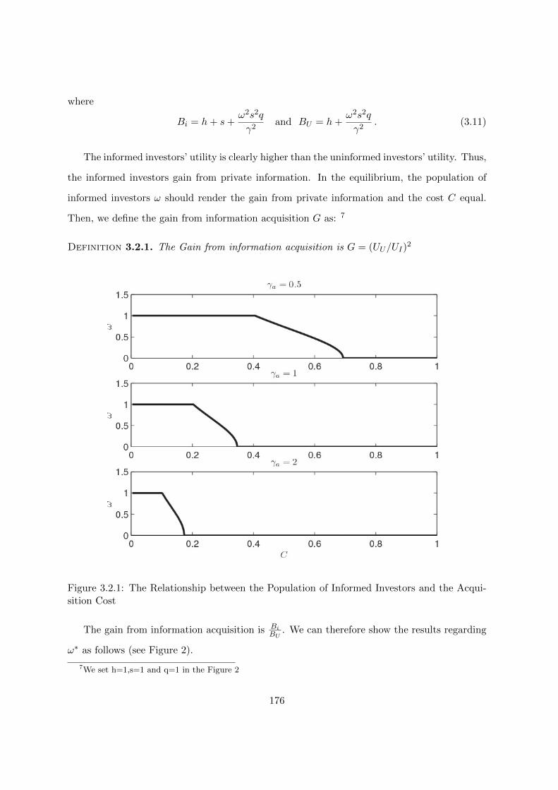
where

Bi = h+ s+ω2s2q

γ2and BU = h+

ω2s2q

γ2. (3.11)

The informed investors’ utility is clearly higher than the uninformed investors’ utility. Thus,

the informed investors gain from private information. In the equilibrium, the population of

informed investors ω should render the gain from private information and the cost C equal.

Then, we define the gain from information acquisition G as: 7

Definition 3.2.1. The Gain from information acquisition is G = (UU/UI)2

Figure 3.2.1: The Relationship between the Population of Informed Investors and the Acqui-sition Cost

The gain from information acquisition is BiBU

. We can therefore show the results regarding

ω∗ as follows (see Figure 2).

7We set h=1,s=1 and q=1 in the Figure 2

176

Proposition 3.2.1. In the equilibrium without an options market, the population of informed

investors renders the gain from information acquisition and its cost equal. Then, there are

three cases:

Case 1: If C ≥ Cd1, the equilibrium population of informed investors is ω∗ = 0.

Case 2: If Cd2 < C < Cd1, the equilibrium population of informed investors is ω∗ ∈ (0, 1).

Case 3: If C ≤ Cd2, the equilibrium population of informed investors is ω∗ = 1.

where Cd1 and Cd2 are defined as in the Appendix.

Corollary 3.2.1. When Cd2 < C < Cd1, ω∗ is monotonically decreasing with the information

acquisition cost C.

Based on the equilibrium population of informed investors, we examine the effect of intro-

ducing an options market on ω and the underlying asset in the following sections. Because we

have corner solutions in Case 1 and Case 3, we focus on the Case 2 to conduct the study.

3.3 Introduction of an Option Market

In this section, we analyze the effects an options market on investors’ information acquisition

decisions and the underlying asset. We study the role of the information acquisition cost in the

effects. We first solve a static model with an option markets, and then we extend this static

model to a dynamic model in next section. We demonstrate the robustness of the results.

After an options market in introduced, the investors’ information sets differ from before

the options market is introduced. For informed investor i, his or her information set is Fi =

{Si, P, PCG, PPG}, whereas uninformed investors’ information set is FU = {P, PCG, PPG}. Our

conjecture is that the underlying risky asset’s price is a linear function of fundamental payoff

D and the noisy traders’ demand n. The partially revealing rational expectations equilibrium

regarding P , PCG, PPG and the investors’ demands is described in the following proposition.

Proposition 3.3.1. There exists one equilibrium in T = 0. Equilibrium P and PG are given

177

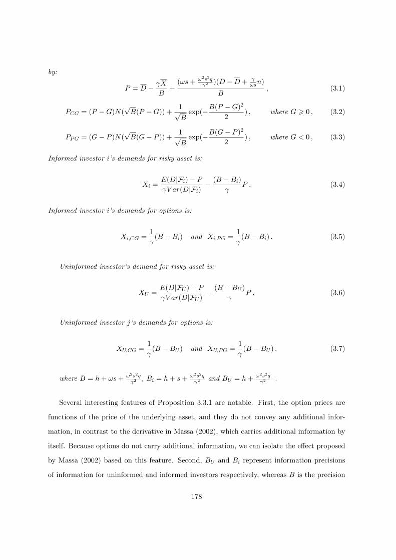
by:

P = D − γX

B+

(ωs+ ω2s2qγ2

)(D −D + γωsn)

B, (3.1)

PCG = (P −G)N(√B(P −G)) +

1√B

exp(−B(P −G)2

2) , where G > 0 , (3.2)

PPG = (G− P )N(√B(G− P )) +

1√B

exp(−B(G− P )2

2) , where G < 0 , (3.3)

Informed investor i’s demands for risky asset is:

Xi =E(D|Fi)− PγV ar(D|Fi)

− (B −Bi)γ

P , (3.4)

Informed investor i’s demands for options is:

Xi,CG =1

γ(B −Bi) and Xi,PG =

1

γ(B −Bi) , (3.5)

Uninformed investor’s demand for risky asset is:

XU =E(D|FU )− PγV ar(D|FU )

− (B −BU )

γP , (3.6)

Uninformed investor j’s demands for options is:

XU,CG =1

γ(B −BU ) and XU,PG =

1

γ(B −BU ) , (3.7)

where B = h+ ωs+ ω2s2qγ2

, Bi = h+ s+ ω2s2qγ2

and BU = h+ ω2s2qγ2

.

Several interesting features of Proposition 3.3.1 are notable. First, the option prices are

functions of the price of the underlying asset, and they do not convey any additional infor-

mation, in contrast to the derivative in Massa (2002), which carries additional information by

itself. Because options do not carry additional information, we can isolate the effect proposed

by Massa (2002) based on this feature. Second, BU and Bi represent information precisions

of information for uninformed and informed investors respectively, whereas B is the precision

178

of the aggregate information. Following the intuition that the value of options depends on

investors’ conditional volatility regarding the underlying asset’s payoff, informed investors’ de-

mand for options is lower than uninformed investors’s demand. In the equilibrium where the

net supply of each option is zero, informed investors are on the short side of options. Thus,

introducing an options market provides an opportunity for informed investors to profit from

selling options. Following the same mechanism, the third feature is that the aggregate option

prices decrease with the precision of aggregate information B, which is shown in the following

Lemma 3.3.1. The analysis implies that options have a similar effect to information in reducing

risk. 8

Lemma 3.3.1. The aggregate price of options is∞∫0

PCGdG+0∫−∞

PPGdG = 12( 1B + P 2).

In line with Grossman and Stiglitz (1980), the equilibrium population of informed investors

renders the expected utility of informed and uninformed investors equal. Before we perform

the comparisons, we must show that there is a unique equilibrium in information acquisition

with an options market. Otherwise, showing the effects of options would be difficult. To

demonstrate the existence of a unique equilibrium, we only need to show that the gain from

information decreases with the population of informed investors ω, which can be shown as

follows.9

Lemma 3.3.2. The gain from information G with an option market is exp( sB ).

The gain from information clearly decreases with the population of informed investors,

which implies that a unique solution exists for information acquisition. However, whether

the equilibrium population of informed investors in the economy with options is higher than

that without options is unclear. Because the information acquisition cost is constant, the

equilibrium population of informed investors is higher in the economy with options if exp( sB )

is higher than BiBU

, and vice versa. Figure 3.3 shows that when the population of informed

investors is zero, exp( sB ) is higher BiBU

. This result indicates that when the population of

8The aggregate payoff of options is: D2 = 2∞∫0

(D −G)+dG+ 20∫−∞

(G−D)+dG.

9We set h=1,s=1, q=1 and γ = 0.5 in the Figure 3

179

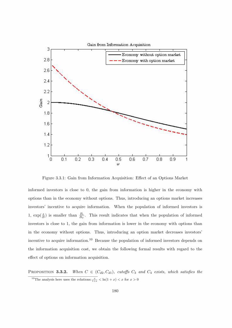
Figure 3.3.1: Gain from Information Acquisition: Effect of an Options Market

informed investors is close to 0, the gain from information is higher in the economy with

options than in the economy without options. Thus, introducing an options market increases

investors’ incentive to acquire information. When the population of informed investors is

1, exp( sB ) is smaller than BiBU

. This result indicates that when the population of informed

investors is close to 1, the gain from information is lower in the economy with options than

in the economy without options. Thus, introducing an option market decreases investors’

incentive to acquire information.10 Because the population of informed investors depends on

the information acquisition cost, we obtain the following formal results with regard to the

effect of options on information acquisition.

Proposition 3.3.2. When C ∈ (Cd2, Cd1), cutoffs C3 and C4 exists, which satisfies the

10The analysis here uses the relations: x1+x

< ln(1 + x) < x for x > 0

180

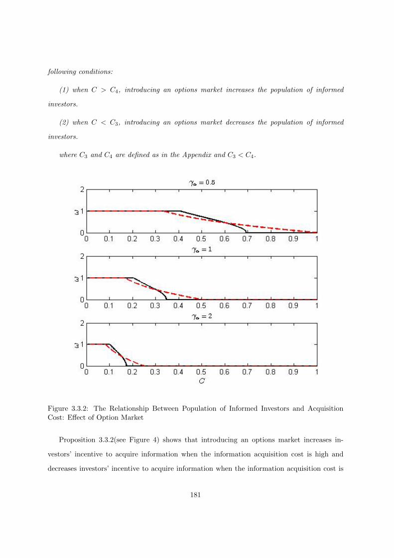
following conditions:

(1) when C > C4, introducing an options market increases the population of informed

investors.

(2) when C < C3, introducing an options market decreases the population of informed

investors.

where C3 and C4 are defined as in the Appendix and C3 < C4.

Figure 3.3.2: The Relationship Between Population of Informed Investors and AcquisitionCost: Effect of Option Market

Proposition 3.3.2(see Figure 4) shows that introducing an options market increases in-

vestors’ incentive to acquire information when the information acquisition cost is high and

decreases investors’ incentive to acquire information when the information acquisition cost is

181

low.11 From the Proposition 3.3.1, we know that the supply of options is higher than the

demand when the population of informed investors is high. Meanwhile, as shown in Lemma

3.3.1, the aggregate option prices tend to be low. The selling profits of informed investors in

the options markets clearly depend on both the demand per supplier and the option prices.

Thus, the profits from selling options are low for informed investors, and they will not cover the

information acquisition cost when the demand is too low. Moreover, investors could use cheap

options instead of information to hedge their portfolios risk, which implies that introducing an

options market decreases investors’ incentive to acquire information. By contrast, the supply

of options is lower than then demand when the population of informed investors is low, leading

to high aggregate option prices. In particular, when the demand per supplier is sufficiently

large, information investors’ profits from selling options will cover the information acquisition

cost, which implies that introducing an options market increases investors’ incentive to acquire

information. Given its effect on information acquisition, the options market has a direct effect

on the price informativeness. To show the effect of options on price informativeness, we define

price informative as follows.

Definition 3.3.1. The price informativeness I: I = 1V ar(D|P ) .

Because the option prices do not convey any additional information, the above definition

of I captures all of the information that is conveyed by the market. Thus we can conveniently

show the effect of options on price informativeness. Price informativeness is clearly ω2s2qγ2

, and

it increases with the population of informed investors. Because introducing an options market

affects the population of informed investors, we obtain the following formal results regarding

price informativeness.

Proposition 3.3.3. When C ∈ (Cd2, Cd1),

(1) when C > C4, introducing an options market increases price informativeness I.

(2) when C < C3, introducing an options market decreases price informativeness I.

where C3 and C4 are defined as in the Appendix and C3 < C4.

11We set h=1,s=1, q=1 in the Figure 4

182

In addition to the effect of options on information acquisition, we also examine their effects

on the price and volatility of the underlying asset. Because uncertainty exists regarding the

asset payoff, the price is discounted. The expected difference between the asset payoff and

price is called the cost of capital: E(D−P ). The cost of capital E(D−P ) decreases with the

expected asset price. Thus the result for expected asset price is equivalent to the analysis on

the cost of capital. The expected asset price is given by:

E(P ) = D − γX

B, (3.8)

and the volatility V (D − P ) is given by:

V ar(D − P ) =1

B+ωs+ γ2q−1

B2. (3.9)

The expected asset price clearly increases with B, and the volatility decreases with B. Thus,

we have the following results:

Proposition 3.3.4. When C ∈ (Cd2, Cd1),

(1) when C > C4, introducing an options market increases the expected asset price and de-

creases the price change volatility.

(2) when C < C3, introducing an options market decreases the expected asset price and in-

creases the price change volatility.

These results arise from the effect of options on information acquisition. When the in-

formation acquisition cost is high, introducing an options market increases the population of

informed investors. Because informed investors have information that is precise, they trade

more aggressively, and they are more willing to absorb noisy supply, which indicates that the

demand for the underlying asset increases, along with a higher expected price level. The price

then becomes less sensitive to noisy supply because increased price informativeness. Conse-

quently, the non-fundamental volatility decreases, leading to decreased total volatility. When

the information acquisition cost is low, a similar mechanism generates the opposite results. In

contrast to the findings of Cao (1999) and Massa (2002), these results imply that the informa-

183

tion acquisition cost plays an important role in the effect of options on asset pricing.

We also examine the effect of the information acquisition cost on the trading volume of

options. The trading volume in the options market is calculated as follows:

Lemma 3.3.3. The trading volume in option market VO = 1γ (

ω∫0

|(Bi−B)|di+(1−ω)|B−BU |) =

2ω(1−ω)sγ .

Because the short side comes from informed investors and long side comes from uninformed

investors in the options market, intuitively, the trading volume is zero when all investors

are informed or uninformed. When the information acquisition cost increases from zero, the

population of uninformed investors increases, which enhances the trading between the different

groups. When the information acquisition cost is sufficiently high, the population of uninformed

investors is high, which makes total total trading volume vanish.

Proposition 3.3.5. The trading volume in the options market exhibits a hump shape as a

function of the information acquisition cost: Vo decreases with the information acquisition cost

when C is higher than CM , and increases with the information acquisition cost when C is lower

than CM ,

where CM is defined as in the Appendix.

3.4 Dynamic Model with an Options Market

This section aims to demonstrate the robustness of the results in Section 3 are robust. More-

over, the dynamic model is helpful for studying the effect of an options market on the price

reaction to public information.

3.4.1 Dynamic model without an Options Market

To model dynamic trading, following Brennan and Cao (1996), we assume that there is an

approximate continuous trading time from T = 0 to T = 1. The trading ends at t, where t is

184

between T = 0 and T = 1. To make the model tractable, we assume that investors can trade

only once in a small time interval z, which means that trading occurs only in the time intervals

[0, z), [z, 2z), [3z, 4z)....[(K − 1)z,Kz), where K is the largest integer satisfying Kz ≤ t. 12

We index the interval [(j − 1)z, jz) by trading round j. Before each trading round j, a public

signal is released. The public signal before trading round j is

Sc,j = D + εc,j , (3.1)

where j = 1, 2....K and εc,j follows normal distribution N(0, 1cjz

). εc,j is independent from

trading rounds and is independent from noise in investors’ private signal. We assume that

z tends to be zero throughout our analysis. This assumption guarantees that the public

information flow is sufficiently smooth and that the price change volatility tends to be zero

between two consecutive trading rounds when the time interval is close to zero. We further

assume that the precision of the aggregate public information until trading round j is Fj , where

Fj =k=j∑k=1

ckz. Therefore, FK is the aggregate precision of public information in this dynamic

model. Furthermore, to simplify the analysis, we assume that there are no additional noisy

traders after the initial trading round. 13

Investors submit their demand schedules conditional on their information sets. The infor-

mation set for informed investor i in trading session j is Fi,j = {Si, Sc,k, Pk, k = 1, 2....j},

whereas the information set for uninformed investors in trading session j is FU,j = {Sc,k, Pk,

k = 1, 2....j}. We assume that investor i submits optimal demand schedule Xi,j in trading

round j. Our conjecture is that the risky asset’s price function is a linear function of fun-

damental payoff D, the noisy traders’ demand n, and public signals. The partially revealing

rational expectations equilibrium is described in the following proposition.

Proposition 3.4.1. Given the population of informed investors ω, one partially revealing

12Here, z is similar to dt in continuous-time model and it captures the feature of fast trading in practice.When z approximates to be zero, this model converges to the continuous-time model in Brennan and Cao (1996)

13Without additional noise traders, it is possible that there are two equilibria (Brennan and Cao, 1996).As argued by Brennan and Cao (1996), one of the equilibria is fully revealing equilibrium and investors makeportfolio choices neither conditional on price nor private information, which is not appealing.

185

rational expectations equilibrium exists, where investors’ demand schedule, investors’ beliefs

and equilibrium prices are given by:

Pj = D − X

Bj+

(ωs+ ω2s2qγ2

)(D −D + γωsn) +

∑jk=1 ckz(Sc,k −D)

Bj, (3.2)

where j = 1, 2....K,K + 1, ...L.

Informed investors’ demand is:

Xi,j =E(D|Fi,j)− PjγV ar(D|Fi,j)

, (3.3)

where

E(D|Fi,j) = D +s(D −D + εi) + ω2s2q

γ2(D −D + γ

ωsn) +∑j

k=1 ckz(Sc,k −D)

h+ s+ ω2s2qγ2

+∑j

k=1 ckz, (3.4)

V ar(D|Fi,j) =1

h+ s+ ω2s2qγ2

+∑j

k=1 ckz, (3.5)

Uninformed investors’ demand is:

XU,j =E(D|FU,j)− PjγV ar(D|FU,j)

, (3.6)

where

E(D|FU,j) = D +

ω2s2qγ2

(D −D + γωsn) +

∑jk=1 ckz(Sc,k −D)

h+ ω2s2qγ2

+∑j

k=1 ckz, (3.7)

V ar(D|FU,j) =1

h+ ω2s2qγ2

+∑j

k=1 ckz, (3.8)

and

Bj = h+ ωs+ω2s2q

γ2+

j∑k=1

ckz . (3.9)

Proposition 3.4.1 shows that the prices only reveal information through D − D + γωsn,

and that the investors behave myopically because there are no additional noisy traders. The

expected utilities of informed and uninformed investors are shown in the following Lemma

186

3.4.1.

Lemma 3.4.1. The expected utility of informed investors in the economy with K trading rounds

is given by

UI = − 1√V ar(D − P1)Bi,1

exp[−γW0 + γC − γX2

2B20V ar(D − P0)

]×j=K∏j=2

1√1 +

cjz(Bj−Bi,j)2Bi,j−1B2

j

,

(3.10)

and the expected utility of uninformed investors is given by

UU = − 1√V ar(D − P1)BU,1

exp[−γW0−γX

2

2B20V ar(D − P0)

]×j=K∏j=2

1√1 +

cjz(Bj−BU,j)2BU,j−1B

2j

. (3.11)

where Bi,j = h+ s+ ω2s2qγ2

+∑j

k=1 ckz, BU,j = h+ ω2s2qγ2

+∑j

k=1 ckz and Bj is defined as

above.

The gain from information G is obviouslyBi,1BU,1

j=N∏j=2

1+cjz(Bj−Bi,j)

2

Bi,j−1B2j

1+cjz(Bj−BU,j)2

BU,j−1B2j

, where1+

cjz(Bj−Bi,j)2

Bi,j−1B2j

1+cjz(Bj−BU,j)2

BU,j−1B2j

is the additional gain generated by trading round j. To provide a further comparison, we

must show that there is a unique equilibrium of information acquisition. Thus, we must show

whether the gain from information decreases with the population of informed investors. We

obtain the following result regarding information acquisition:

Proposition 3.4.2. The gain from information G decreases with the population of informed

investors ω.

Proposition 3.4.2 shows that a unique equilibrium exists. Further, the equilibrium popu-

lation of informed investors decreases with the information acquisition cost, which is shown

below.

187

Corollary 3.4.1. In an economy with K trading rounds, the population of informed investors

renders the gain from information and the information acquisition cost equal. There are three

cases:

Case 1: If C ≥ C1, the equilibrium population of informed investors ω∗ = 0.

Case 2: If C2 < C < C1, the equilibrium population of informed investors ω∗ ∈ (0, 1).

Case 3: If C ≤ C2,the equilibrium population of informed investors ω∗ = 1.

where C1 and C2 are defined as in the Appendix.

Corollary 3.4.2. When C2 < C < C1, ω∗ decreases with the information acquisition cost

C.

Given the information acquisition cost C, we show how the precision of public information

FK affects the equilibrium population of informed investors ω in the following results.

Corollary 3.4.3. In an economy with K trading rounds, the population of informed investors

renders the gain from information and the information acquisition cost equal. There are three

cases:

Case 1: If FK ≥ F1, the equilibrium population of informed investors ω∗ = 0.

Case 2: If F2 < FK < F1, the equilibrium population of informed investors ω∗ ∈ (0, 1).

Case 3: If FK ≤ F2,the equilibrium population of informed investors ω∗ = 1.

where F1 and F2 are defined in the Appendix.

Corollary 3.4.4. When F2 < FK < F1, ω∗ decreases with the public information precision

Fk.

Corollary 3.4.3 intuitively indicates that investors’ incentive to acquire private information

decreases with the precision of public information owing to the decreasing marginal benefit of

information. Because there are corner solutions in Case 1 and Case 3, we focus on the Case 2

to perform the analysis regarding the public information.

188

3.4.2 Dynamic model with an options market

In this section, we solve a dynamic model with an options market to demonstrate that the

robustness of the results regarding the effects of options on information acquisition and the

underlying asset from the static model. Furthermore, we show the effect of an options market

on price reactions to public information.

We introduce an options market, that consists of a section of call and put options, as in Sec-

tion 3. Let Pk be the risky asset’s price in trading round k, PCG,k be the price for a call option

with strike price G, and PPG,k be the price for a put option with strike price G. The infor-

mation set for For informed investor i in trading round j is Fi,j = {Si, Sc,k, Pk, PCG,k, PPG,k,

k = 1, 2....j}, whereas the information set for uninformed investors in trading round j is

FU,j = {Sc,k, Pk, PCG,k, PPG,k, k = 1, 2....j}. We assume that investor i submits optimal de-

mand schedule Xi,j for the risky asset, Xi,CG,j for call option with strike price G, and Xi,PG,j

for put option with strike price G in trading round j. Our conjecture is that the underlying

asset’s price function is a linear function of fundamental payoff D, the noisy trader n, and

public signals. The partially revealing rational expectations equilibrium is described in the

following proposition.

Proposition 3.4.3. Given the population of informed investors ω, one partially revealing

rational expectations equilibrium exists, where investors’ demand schedule, investors’ beliefs

and equilibrium prices are given by:

Pj = D − γX

Bj+

(ωs+ ω2s2qγ2

)(D −D + γωsn) +

∑jk=1 ckz(Sc,k −D)

Bj, (3.12)

PCG,j = (Pj −G)N(√Bj(Pj −G)) +

1√Bj

exp(−Bj(Pj −G)2

2) where G > 0 , (3.13)

PPG,j = (G− Pj)N(√Bj(G− Pj)) +

1√Bj

exp(−Bj(G− Pj)2

2) where G < 0 , (3.14)

where j = 1, 2....K.

189

Informed investors’ demand for the underlying asset is:

Xi,j =E(D|Fi,j)− PjγV ar(D|Fi,j)

− (Bj −Bi,j)γ

Pj , (3.15)

Informed investors’ demand for options is

Xi,CG,j =1

2γ(Bj −Bi,j) and Xi,PG,j =

1

2γ(Bj −Bi,j) , (3.16)

Uninformed investors’ demand for the underlying asset is:

XU,j =E(D|FU,j)− PjγV ar(D|FU,j)

−(Bj −BU,j)

γPj , (3.17)

Uninformed investors’ demand for options is

XU,CG,j =1

2γ(Bj −BU,j) and XU,PG,j =

1

2γ(Bj −BU,j) . (3.18)

where Bj = ωBi,j + (1− ω)BU,j, Bi,j = h+ s+ ω2s2qγ2 +

∑jk=1 ckz and BU,j = h+ ω2s2q

γ2 +∑jk=1 ckz

Proposition 3.4.3 shows that investors’ optimal demands for the underlying asset and op-

tions are similar to that found in the static model. An interesting finding is that option prices

only depend on the price of the underlying asset, and that they do not convey any additional

information. Regarding investors’ utility, we obtain the following lemma

Lemma 3.4.2. Informed investor i’s expected utility in trading round j is

EVi,j = − 1√BjBi,j

E{exp[−γWi,j −[E(D|Fi,j+1)− Pj+1]

2

2γV ar(D|Fi,j+1)+Bj −Bi,j

2

1

Bj]} , (3.19)

and uninformed investors’ expected utility in trading round j is:

190

EVU,j = − 1√BjBU,j

E{exp[−γWU,j −[E(D|FU,j+1)− Pj+1]

2

2γV ar(D|FU,j+1)+Bj −BU,j

2

1

Bj]} . (3.20)

Lemma 3.4.2 shows that the gain from information is exp( sB ), where B = h+ ωs+ ω2s2qγ2

.

Further, this gain decreases with the population of informed investors. Thus, a unique interior

solution exists to render the gain from information and the cost equal. To conduct the analysis

over the expected asset price and price change volatility, we know that the expected price is

given by

E(Pj) = D − γX

Bj, (3.21)

The price change volatility is given by

V ar(Pj+1 − Pj) =1

Bj− 1

Bj+1+

c2j+1

B2jB

2j+1

(ωs+γ2

q), (3.22)

and the price informativeness is given by

I =1

V ar(D|Pj). (3.23)

We demonstrate the robustness of the effects of options on information acquisition and the

underlying asset in the dynamic model as follows.

Proposition 3.4.4. When C ∈ (C2, C1), cutoffs C3 and C4 exists, which satisfies the follow-

ing condition:

(1) When C > C4, introducing an options market increases the population of informed

investors, increases price informativeness, increases the expected asset price, and decreases

price change volatility.

(2) When C < C3, introducing an options market decreases the population of informed

investors, decreases price informativeness, decreases the expected asset price, and increases

191

price change volatility.

where C3 and C4 are defined as in the Appendix and C3 < C4.

Findings regarding price reactions to earnings announcements in the U.S. market are also

conflicting, as previous studies suggest that options listing decreased earnings announcements’

surprise before 1980 (Jennings and Starks, 1986, Skinner, 1990, Damodaran, 1991 and Ho,

1993), but increases earnings announcements’ surprise after 1980 (Mendenhall and Fehrs, 1999).

The proxy for the price reactions to public information in trading round j iscjzBj

, which decreases

with Bj . When investors have more information about fundamental value, intuitively, the

surprise to earnings announcements would be smaller. The result presented below shows

that the effect of options listing on the price reactions to public information depends on the

information acquisition cost. This result also differs from that by Cao (1999), who concludes

that options listing decreases price reactions to public information.

Proposition 3.4.5. When C ∈ (C2, C1),

(1) When C > C4, introducing an options market decreases price reactions to public infor-

mation.

(2) When C < C3, introducing an options market increases price reactions to public infor-

mation.

where C3 and C4 are defined as in the Appendix and C3 < C4.

As shown in Corollary 3.4.3, the precision of public information also affects investors’ incen-

tive to acquire information. Thus, we can expect the effect of an options market on information

acquisition and asset prices to depend on the precision of public information. According to

Proposition 3.4.6, the effects of options in the economy with precise public information are

similar to those with high information acquisition costs, whereas the effects of options in an

economy with imprecise public information are similar to those with low information acqui-

sition costs. The population of informed investors is low when public information is precise

before the introduction of options, which leads to a high demand for options and high option

192

prices. Introducing an options market then provides informed investors with an opportunity

to earn profits from selling options to cover the information acquisition cost, which increases

investors’ incentive to acquire information. When public information is imprecise, the popula-

tion of informed investors is high, leading to low option prices. Thus, investors can use cheap

options instead of information to reduce risk, which lowers investors’ incentives to acquire

information.

Proposition 3.4.6. When FK ∈ (F2, F1),

(1) When FK > F4, introducing an options market increases investors’ incentive to acquire

information, increases price informativeness, increases the expected asset price and decreases

price change volatility.

(2) When FK < F3, introducing an options market decreases investors’ incentive to acquire

information, decreases price informativeness, decreases the expected asset price and increases

price change volatility.

where F3 and F4 are defined as in the Appendix and F3 < F4.

3.4.3 Effect of additional trading rounds

As argued by Brennan and Cao (1996), additional trading rounds have a similar effect to

derivatives in improving investors’ welfare. However, whether additional trading rounds have

similar effects to an option market in affecting investors’ incentive to acquire information is

unclear. This issue is important because it has important implications on the after-hour or

round-the-clock trading, which is associated high operational costs. This section formally

addresses this question.

We assume that introducing additional trading rounds increases trading time from t to s,

where s > t. The increase in trading time from t to s can be interpreted as after-hour or

round-the-clock trading. Additional trading time increases the number of time intervals and

the last time interval is [(L−1)z, Lz), where L is the largest integer satisfying Lz ≤ s.14 Before

14This modeling about after-hour or round-the-clock trading is similar to Brennan and Cao (1996). The only

193

each trading round, a public signal is released. The public signal before trading round j is

Sc,j = D + εc,j , (3.24)

where j = 1, 2....K,K+1, ...L and εc,j follows normal distribution N(0, 1cjz

). εc,j is independent

cross trading sessions and is independent of noise in investors’ private signal. The analysis

follows the dynamic model without options. The expected utilities of informed investors and

uninformed investors in the economy with additional trading rounds are given by:

The expected utility of informed investors is:

UI = − 1√V ar(D − P1)Bi,1

exp[−γW0 + γC − γX2

2B20V ar(D − P0)

]×j=L∏j=2

1√1 +

cjz(Bj−Bi,j)2Bi,j−1B2

j

,

(3.25)

and the expected utility of uninformed investors is:

UU = − 1√V ar(D − P1)BU,1

exp[−γW0−γX

2

2B20V ar(D − P0)

]×j=L∏j=2

1√1 +

cjz(Bj−BU,j)2BU,j−1B

2j

, (3.26)

where Bi,j = h+ s+ ω2s2qγ2

+∑j

k=1 ckz, BU,j = h+ ω2s2qγ2

+∑j

k=1 ckz and Bj is defined as

above

It is obvious that gain ∆G from additional trading rounds isBi,1BU,1

j=L∏j=K+1

1+cjz(Bj−Bi,j)

2

Bi,j−1B2j

1+cjz(Bj−BU,j)2

BU,j−1B2j

. If

∆G is larger than 1, additional trading rounds provide a greater benefit to informed investors

than uninformed ones. Then, investors have a greater incentive to acquire information after

the introduction of additional trading rounds. If ∆G is less than 1, additional trading rounds

decrease investors’ incentive to acquire information. Proposition 3.4.7 shows that additional

trading opportunities encourage more investors to acquire information when the information

difference is that we assume there are approximate continuous trading times, while they assume discrete tradingsessions.

194

cost is high, but discourage investors from acquiring information when this cost is low. Al-

though additional trading opportunities improve the welfare of all investors (Brennan and

Cao, 1996) owing to more risk-sharing opportunities, the benefits are asymmetric for different

groups. When the population of informed investors is high because of low information acquisi-

tion costs, this additional benefit is low for informed investors because of the high competition

within this group, whereas the benefit is high for uninformed investors. Thus, investors’ incen-

tive to acquire information is diminished and the equilibrium population of informed investors

is reduced. When the cost is high, the opposite effect arises.

Proposition 3.4.7. When C ∈ (C2, C1),

(1) When C > C4, introducing additional trading rounds increases the population of informed

investors, increases price informativeness, increases the expected asset price, decreases price

change volatility and decrease price reactions to public information.

(2) When C < C3, introducing additional trading rounds decreases the population of in-

formed investors, decreases price informativeness, decreases expected asset price, increases

price change volatility and increases price reactions to public information.

where C3 and C4 are defined in the Appendix and C3 < C4.

3.5 Discussion

The previous sections focus on the analysis of an options market. Considering some general

derivatives is also interesting. Thus, this section provides a further analysis of the derivatives

that are modeled by Cao (1999) and shows that our main mechanism is robust to the use of

derivatives other than options.

Following Cao (1999), we assume that a derivative asset’s payoff is a function of D and

P . The specific function is denoted by g(|D − P |), where g(·) is a monotonic function. We

assume that informed investor i’s demand for this derivative is XGi, and uninformed investors’

demand for this derivative is XGU . Moreover, the equilibrium price of this derivative is denoted

195

by PG. Following Cao (1999), we obtain the following results regarding investors’ demand and

equilibrium prices:

P = D − γX

B+

(ωs+ ω2s2qγ2

)(D −D + γωsn)

B, (3.27)

Informed investor i’s demand is:

Xi =E(D|Fi)− PγV ar(D|Fi)

, (3.28)

Uninformed investors’ demand is:

XU =E(D|FU )− PγV ar(D|FU )

, (3.29)

Informed investors’ demand for the derivative satisfies:

∫ +∞

0(g(y)− PG) exp[−Biy2/2− γXGig(y)]dy = 0 , (3.30)

Uninformed investors’ demand for the derivative satisfies:

∫ +∞

0(g(y)− PG) exp[−BUy2/2− γXGUg(y)]dy = 0 , (3.31)

The market clearing condition is:

ωXGi + (1− ω)XGU = 0 (3.32)

Then, the expected utility of informed investors is:

UGI = UI

√2

πBi

∫ +∞

0exp[−BIy2/2− γ(XGi − PG)g(y)]dy, (3.33)

196

UGU = UU

√2

πBU

∫ +∞

0exp[−BUy2/2− γ(XGU − PG)g(y)]dy, (3.34)

We know the gain from information with this derivative is G = (UGU /UGI )2. Because

obtaining analytical solutions is difficult, we rely on numerical studies. In the numerical studies,

we consider two special cases for g(·): first, g(y) = y; second, g(y) = y2. In particular, we

compare the gain from information in the economy with and without this derivative, given the

population of informed investors. The results are illustrated in Figure 5 and Figure 6.15 The

gain from information is clearly larger in the economy with derivatives than in that without

derivatives when the population of informed investors is small. The opposite results is obtained

when the population of informed investors is large.

3.6 Conclusions

This paper examines the effect of introducing an options market on investors’ incentive to

acquire private information and the pricing behaviour of the underlying asset. As a novel find-

ing, this paper demonstrates that introducing an options market increases investors’ incentive

to acquire private information when the information acquisition cost is high, but decreases

their incentive to acquire private information when the cost is low. Consequently, when the

information acquisition cost is high, an options market increases the underlying asset’s price

informativeness, increases the expected asset price, decreases price volatility and decreases

market responses to earnings announcements. By contrast, when the information acquisition

cost is low, the opposite effects arise. These results can provide a potentially unified theory

for the conflicting findings on the effect of options listing in the U.S. market and international

markets.

15The detailed proof can be found in Cao (1999). We set h=1,s=1, q=1 and γ = 0.5 in the Figure 5 andFigure 6

197

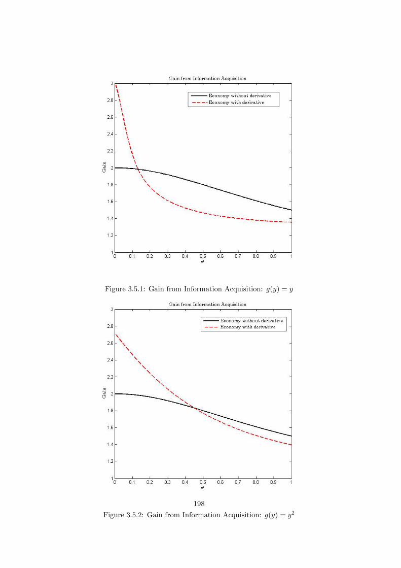
Figure 3.5.1: Gain from Information Acquisition: g(y) = y

Figure 3.5.2: Gain from Information Acquisition: g(y) = y2198

Moreover, this paper also provides some innovative predictions: First, although we do not

formally study the effect of options listing on market liquidity, this paper predicts that an

options market increases the liquidity of the underlying asset market in an illiquid market and

decreases liquidity in a liquid market. When the population of informed investors is high,

price is less sensitive to noisy supply, reducing the price impact of the noisy supply. Thus,

the market has high liquidity. As shown above, a large population of informed investors leads

to a higher supply for options than demand, which is associated with low option prices and

low profits from selling options. Introducing an options market decreases investors’ incentive

to acquire information, which results in lower price informativeness. Consequently, the price

impact of the noisy supply increases and market liquidity deteriorates. Opposite effect of

options listing arises in illiquid market with a small population of informed investors. This

is consistent with the findings by Fedenia and Grammatikos (1992). Second, options listing

has stabilizing effect (increasing price informativeness, raising asset price, decreasing price

volatility and market reactions to earnings announcements) when the public information is

precise, but has destabilization effect (decreasing price informativeness, decreasing asset price,

increasing price volatility and market responses to earnings announcements) when the public

information is imprecise. third, introducing an options market and implementing after-hour

or round-the-clock trading have stabilizing effects (improving informational efficiency, decreas-

ing price volatility) on the underlying assets with high information acquisition costs, such as

small firms and firms with low analyst coverage; Fourth, introducing an options market and

implementing after-hour or round-the-clock trading have destabilization effects (harming infor-

mational efficiency, increasing price volatility) on the underlying assets with low information

acquisition costs, such as large or well-known firms and firms with high analyst coverage.

Although previous theoretical studies on derivatives find that introducing derivatives in-

crease asset prices and decrease price volatilities (Cao, 1999 and Massa, 2002), these studies

can not reconcile the findings: options listing increases asset prices, decreases price volatility

and decreases price reactions to earning announcements in U.S. market before 1980, but yields

the opposite effects after 1980. Further, these studies can not explain the findings: options

199

listing tends to have stabilizing effects in emerging markets, such as India, but have desta-

bilization effects in some developed markets, such as Germany. Our results not only explain

these conflicting facts regarding the effects of options listing, but also shed new light on debates

about whether a derivative market has (de)stabilizing effects on the underlying asset market.

Because we aim to obtain tractable solutions, our model assumes that there are no addi-

tional noisy traders after the initial trading round in the dynamic model. However, extending

our model to consider time-varying noisy traders may provide an interesting future research

avenue. Such as extension would also be useful for studying market liquidity in a general dy-

namic model. In addition, future research may study the effect of other financial innovations

on investors’ incentive to acquire information, as in the study by Simsek (2013a,b). More

important, we notice that the options have no direct impact on underlying assets because

of the assumptions of CARA utility and normal distributions. Although this feature helps

to elucidate the effects of options on information acquisition, relaxing these assumptions and

analyzing the effects derivatives on asset prices under general utility functions may provide a

fruitful research avenue. We leave all of these to further studies.

200

Bibliography

Admati, Anat R, 1985, A Noisy Rational Expectations Equilibrium for Multi-Asset Securities Mar-

kets, Econometrica, 53, 629-657.

Admati, Anat R and Paul Pfleiderer, 1988, Selling and Trading on Information In Financial

Markets, American Economic Review, 78, 96-103.

Allen, Franklin and Douglas Gale, 1994, Financial Innovation and Risk Sharing, MIT Press,

Cambridge, Mass.

Akerlof, George A, 1970, The Market for ”Lemons”: Quality Uncertainty and the Market Mecha-

nism, Quarterly Journal of Economics, 84, 488-500.

Back, Kerry, 1993, Asymmetric Information and Options, Review of Financial Studies, 3:1-24.

Bansal, Vipul K, Stephen W. Pruitt and K.C. John Wei, 1989, An Empirical Reexaminaiton

of the Impact of CBOE Option Initiaiton on the Volatility and Trading Volume of the Underlying

Equities: 1973-1986, Financial Review, 24, 19-29.

Bhattacharya, Utpal, Philip J. Reny and Matthew Spiegel, 1995, Destructive Interference

In An Imperfectly Competitive Multi-Security Market, Journal of Economic Theory, 65, 136-170.

Bollen, Nocolas P.B, 1998, A Note on the Impact of Options on Stock Return Volatility, Journal

of Banking and Finance, 22, 1181-1191.

Branch, Ben and Joseph E. Finnerty, 1981, The Impact of Option Listing On the Price and

Volume of the Underlying Stock, Financial Review, 16, 1-15.

Breeden, Douglas, 1984, Futures Markets and Commodity Options: Hedging and Optimality in

Incomplete Markets, Journal of Economic Theory, 32, 275-300.

201

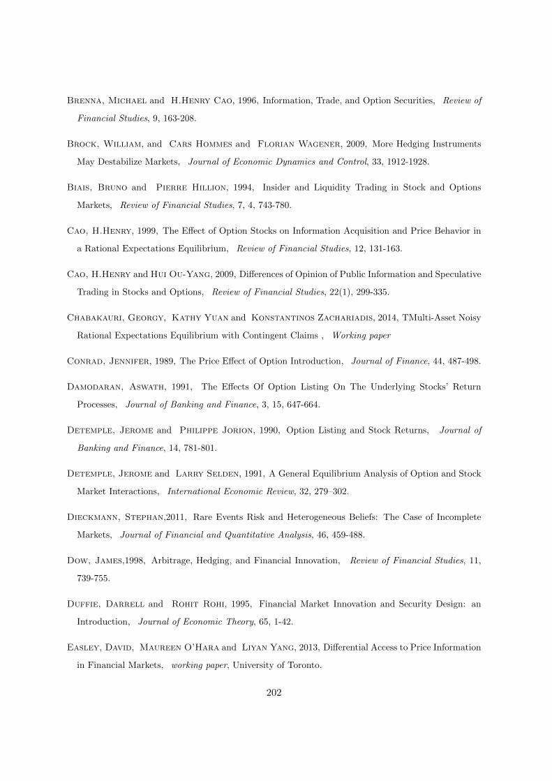
Brenna, Michael and H.Henry Cao, 1996, Information, Trade, and Option Securities, Review of

Financial Studies, 9, 163-208.

Brock, William, and Cars Hommes and Florian Wagener, 2009, More Hedging Instruments

May Destabilize Markets, Journal of Economic Dynamics and Control, 33, 1912-1928.

Biais, Bruno and Pierre Hillion, 1994, Insider and Liquidity Trading in Stock and Options

Markets, Review of Financial Studies, 7, 4, 743-780.

Cao, H.Henry, 1999, The Effect of Option Stocks on Information Acquisition and Price Behavior in

a Rational Expectations Equilibrium, Review of Financial Studies, 12, 131-163.

Cao, H.Henry and Hui Ou-Yang, 2009, Differences of Opinion of Public Information and Speculative

Trading in Stocks and Options, Review of Financial Studies, 22(1), 299-335.

Chabakauri, Georgy, Kathy Yuan and Konstantinos Zachariadis, 2014, TMulti-Asset Noisy

Rational Expectations Equilibrium with Contingent Claims , Working paper

Conrad, Jennifer, 1989, The Price Effect of Option Introduction, Journal of Finance, 44, 487-498.

Damodaran, Aswath, 1991, The Effects Of Option Listing On The Underlying Stocks’ Return

Processes, Journal of Banking and Finance, 3, 15, 647-664.

Detemple, Jerome and Philippe Jorion, 1990, Option Listing and Stock Returns, Journal of

Banking and Finance, 14, 781-801.

Detemple, Jerome and Larry Selden, 1991, A General Equilibrium Analysis of Option and Stock

Market Interactions, International Economic Review, 32, 279–302.

Dieckmann, Stephan,2011, Rare Events Risk and Heterogeneous Beliefs: The Case of Incomplete

Markets, Journal of Financial and Quantitative Analysis, 46, 459-488.

Dow, James,1998, Arbitrage, Hedging, and Financial Innovation, Review of Financial Studies, 11,

739-755.

Duffie, Darrell and Rohit Rohi, 1995, Financial Market Innovation and Security Design: an

Introduction, Journal of Economic Theory, 65, 1-42.

Easley, David, Maureen O’Hara and Liyan Yang, 2013, Differential Access to Price Information

in Financial Markets, working paper, University of Toronto.

202

Edwards, Franklin R., 1998a, Futures Trading and cash Market Volatility: Stock Index and Interest

Rate Futures, Journal of Future Markets, 44, 63-68.

Edwards, Franklin R., 1998b, Does Futures Trading Increase Stock Market Volatility?, Financial

Analyst Journal, 8, 421-439.

Fedenia, Mark and Theoharry Grammatikos, 1992, Options Trading and the Bid-Ask Spread

on the Underlying Stocks, Journal of Business, 65, 335-351.

Freund, Steven, P. Douglas McCann and Gwendolyn P. Webb, 1994, A Regression Analysis

of the Effects of Option Introduction on Stock Variances, Journal of Derivatives, 1, 25-38.

Galloway, Tina M. and James M. Miller, 1997, Index Futures Trading and Stock Return

Volatility: Evidence From the Introduction of MidCap 400 Index Futures, Financial Review, 32,

845-866.

Grossman, Sanford, 1976, On The Efficiency Of Competitive Stock Markets When Traders Have

Diverse Information, Journal of Finance, 31, 573-585.

Grossman, Sanford, 1988, An Analysis of the Implication for Stock and Futures Price Volatility of

Program Trading and Dynamic Hedging Strategies, Journal of Business, 61, 275-298.

Grossman, Sanford, and Merton Miller, 1988, Liquidity And Market Structure, Journal of

Finance, 43, 617-637.

Grossman, Sanford, and Joseph Stiglitz, 1980, On The Impossibility Of Informationnaly Efficient

Markets, American Economic Review, 70, 393-408.

Grundy, Bruce, and Maureen McNichols, 1989, Trade And The Revelation Of Information

Through Prices And Direct Disclosure, Review of Financial Studies, 2, 495-526.

Guesnerie, Roger, 1993, (De)Stabilizing Speculation on Futures Markets: An Alternative View

Point, European Economic Review, 37, 1043-1063.

Hamill, Philip A, Kwaku K. Opong,and Pat McGregor, 2002, Equity Option Listing in the

UK: A Comparison Of market-Based Research Methodologies, Journal of Empirical Finance, 9, 1,

91-108.

Hayes, Samuel L, and Michale E. Tennenhaum, 1979, The Impact of Listed Options on the

Underlying Shares, Financial Management, 8, 72-76.

203

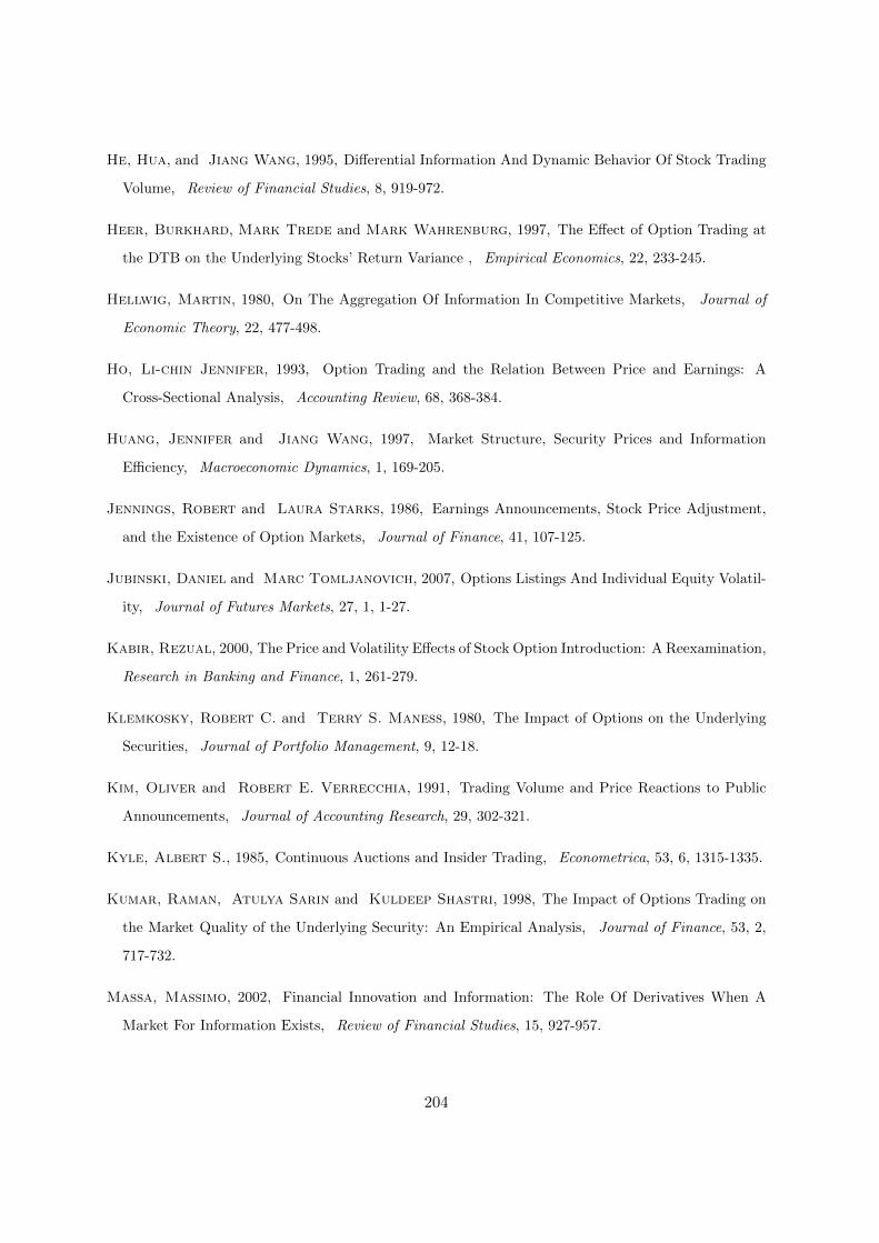
He, Hua, and Jiang Wang, 1995, Differential Information And Dynamic Behavior Of Stock Trading

Volume, Review of Financial Studies, 8, 919-972.

Heer, Burkhard, Mark Trede and Mark Wahrenburg, 1997, The Effect of Option Trading at

the DTB on the Underlying Stocks’ Return Variance , Empirical Economics, 22, 233-245.

Hellwig, Martin, 1980, On The Aggregation Of Information In Competitive Markets, Journal of

Economic Theory, 22, 477-498.

Ho, Li-chin Jennifer, 1993, Option Trading and the Relation Between Price and Earnings: A

Cross-Sectional Analysis, Accounting Review, 68, 368-384.

Huang, Jennifer and Jiang Wang, 1997, Market Structure, Security Prices and Information

Efficiency, Macroeconomic Dynamics, 1, 169-205.

Jennings, Robert and Laura Starks, 1986, Earnings Announcements, Stock Price Adjustment,

and the Existence of Option Markets, Journal of Finance, 41, 107-125.

Jubinski, Daniel and Marc Tomljanovich, 2007, Options Listings And Individual Equity Volatil-

ity, Journal of Futures Markets, 27, 1, 1-27.

Kabir, Rezual, 2000, The Price and Volatility Effects of Stock Option Introduction: A Reexamination,

Research in Banking and Finance, 1, 261-279.

Klemkosky, Robert C. and Terry S. Maness, 1980, The Impact of Options on the Underlying

Securities, Journal of Portfolio Management, 9, 12-18.

Kim, Oliver and Robert E. Verrecchia, 1991, Trading Volume and Price Reactions to Public

Announcements, Journal of Accounting Research, 29, 302-321.

Kyle, Albert S., 1985, Continuous Auctions and Insider Trading, Econometrica, 53, 6, 1315-1335.

Kumar, Raman, Atulya Sarin and Kuldeep Shastri, 1998, The Impact of Options Trading on

the Market Quality of the Underlying Security: An Empirical Analysis, Journal of Finance, 53, 2,

717-732.

Massa, Massimo, 2002, Financial Innovation and Information: The Role Of Derivatives When A

Market For Information Exists, Review of Financial Studies, 15, 927-957.

204

Mayhew, Stewart and Vassil Mihov, 2000, Another Look at Option Listing Effects, working

paper.

Mendenhall, Richard R. and Donald H. Fehrs, 1999, Option Listing and the Stock-Price

Response to Earnings Announcements, Journal of Accounting and Economics, 27, 57-87.

Nair, S.Abhilash, 2008, Impact Of Derivative Trading on Volatility of the Underlying: Evidence

from Indian Stock Market, working paper, Conference On Money And Finance 2008, Mumbai

Rao, Ramesh P. and Christopher K. Ma, 1987, The Effect of Call-Option-Listing Announcement

on Shareholder Wealth, Journal of Business Research, 15, 449-465.

Ross, Stephen A., 1976, Options and Efficiency, Quarterly Journal of Economics, 90, 75-89.

Simsek, Alp, 2013a, Speculation and Risk Sharing with New Financial Assets, Quarterly Journal of

Economics, 128-3, 1365-1396.

Simsek, Alp, 2013b, Financial Innovation and Portfolio Risks, American Economic Review Papers

and Proceedings, 103-3, 398-401.

Skinner, Douglas, 1989, Options Market ans Stock Return Volatility, Journal of Financial Eco-

nomics, 23, 61-78.

Skinner, Douglas, 1990, Options Markets and the Informaiton Content of Accounting Earnings

Release, Journal of Accounting And Economics, 13, 191-211.

Sorescu, Sorin M., 2000, The Effect of Options on Stock Prices: 1973-1995, The Journal of Finance,

55, 1, 487-514.

Subrahmanyam, Avanidhar, 1992, Risk Aversion, Market Liquidity, and Price Efficiency, The

Review of Financial Studies, 4, 3, 417-441.

Swan, Edward J., 2000, Building the Global Market, a 4000 Year History of Derivatives, Kluwer

Law International, Boston.

Stephan, Jens A., and Robert E. Whaley, 1990, Intraday Price Change and Trading Volume

Relations in the Stock and Stock Option Markets, The Journal of Finance, 45, 191-220.

Stroll, Hans, 1978a, The Pricing of Security Dealer Services: An Empirical Study Of NASDAQ

Stocks, The Journal of Finance, 33, 1153-1172.

205

Stroll, Hans, 1978b, The Supply Of Dealer Services In Securities Markets, The Journal of Finance,

33, 1133-1151.

Wang, Jiang, 1993, A Model Of Intertemporal Asset Prices Under Asymmetric Information, Review

of Economics Studies, 60, 249-282.

Wang, Jiang, 1994, A Model Of Competitive Stock Trading Volume, Journal of Political Economy,

102, 127-168.

Weyl, Glen, 2007, Is Arbitrage Socially Beneficial,2007 Princeton University working paper.

206

3.7 Appendix

This appendix provides all proofs omitted above.

Proof of Proposition 3.2.1.

EVi = − exp[−γW0 −X

2

2γB2V ar(D − P )]× 1√

V ar(D − P )Bi(3.1)

EVU = − exp[−γW0 −X

2

2γB2V ar(D − P )]× 1√

V ar(D − P )BU(3.2)

The Gain G in the case without derivative security is BiBU

. In the equilibrium, investors should

break even the gain from information acquisition and cost. If G(0) ≤ exp(2γC), the equilibrium

fraction of informed investors ω∗ = 0. If G(0) > exp(2γC) > G(1), the equilibrium fraction

of informed investors ω∗ ∈ (0, 1) which satisfies G(ω∗) = exp(2γC). If exp(2γC) ≤ G(1),the

equilibrium fraction of informed investors ω∗ = 1.. Therefore, we can get the lemma. And

Cd1 satisfy G(0) = exp(2γCd1) and Cd2 satisfy G(1) = exp(2γCd2). Since G is a decreasing

function of ω, it is obvious that ω∗ is a decreasing function with C when Cd2 < C < Cd1

Proof of Proposition 3.3.1 and Proof of Lemma 3.3.1. To prove that price function and

demands are in the equilibrium, we should prove that the market is clearing in the equilibrium

and Euler condition holds for the demand of different assets. Given the informed investors and

uninformed investors’ demand of the risky assset and options, we have the following market

clearing condition:

for the stock, we have

ωXi + (1− ω)XU + n = X (3.3)

It is clear that the price in the proposition clears the market of the risky asset.

207

for the options, we have

ω

γ(B −Bi) + (1− ω)(B −BU ) = 0 (3.4)

Since B = h+ ωs+ ω2s2qγ2

+ c, it is clear that the option market is clearing.

Next we will show the Euler condition holds for the demand of different assets. For informed

investor i’s final wealth is given by:

Wi,1 = Wi,0+Xi(D−P )+

∞∫0

Xi,CG[(D−G)+−PCG]dG+

0∫−∞

Xi,PG[(G−D)+−PPG]dG (3.5)

Given the equilibrium Xi,CG and Xi,PG, we firstly prove that the proposed demand of risky

asset satisfies the first order condition for investors’ optimization problem.

Due to D2 = 2∞∫0

(D −G)+dG+ 20∫−∞

(G−D)+dG, we have

Wi,1 = Wi,0 +Xi(D − P ) +B −Biγ

D2

2− B −Bi

γ(

∞∫0

PCGdG+

0∫−∞

PPG]dG) (3.6)

Informed investors maximize expected utility

−E{exp(−γWi,1)|Fi}

= −E{exp[−γ(Wi,0 +Xi(D − P ) + B−Biγ

D2

2 −B−Biγ (

∞∫0

PCGdG+0∫−∞

PPG]dG))]|Fi}

= − 1√1+(B−Bi) 1

Bi

exp[−γWi,0 + (B −Bi)(∞∫0

PCGdG+0∫−∞

PPG]dG))] + γXiP − γXiE(D|Fi)

−B−Bi2 E2(D|Fi) + 1

2(γXi + (B −Bi)E(D|Fi))2 1Bi

11+(B−Bi) 1

Bi

]

(3.7)

FOC, we have: γP − γE(D|Fi) + (γXi + (B−Bi)E(D|Fi)) γB = 0⇒ Xi = Biγ (E(D|Fi)−P )−

1γ (B −Bi)P

This proves that the proposed demand of risky asset satisfies the first order condition for

208

investors’ optimization problem. Now we show that proposed demands and prices for the

options satisfy the Euler conditions. This means that we need to prove that:

E[((D −G)+ − PCG) exp(−γWi,1)|Fi] = 0 E[((G−D)+ − PPG) exp(−γWi,1)|Fi] = 0

(3.8)

Since∫ +∞0 (P −G)N(

√B(P −G))dG+

∫ +∞0

1√B

exp(−B(P−G)2

2 )dG+∫ 0∞(G− P )N(

√B(G−

P ))dG+∫ +∞0

1√B

exp(−B(G−P )2

2 )dG

=∫ +∞0 (P −G)N(

√B(P −G))dG+

∫ 0∞(G− P )N(

√B(G− P ))dG+ 1

B

=∫ +∞0 (P −G)

∫ √B(P−G)−∞

1√2π

exp(−12x

2)dxdG

+∫ 0−∞(G− P )

∫ √B(G−P )−∞

1√2π

exp(−12x

2)dxdG+ 1B

=∫ P√B−∞

1√2π

∫ P− x√B

0 (P−G)dG exp(−12x

2)dx+∫ −P√B−∞

1√2π

∫ 0P+ x√

B

(G−P )dG exp(−12x

2)dx+

1B

=∫ P√B−∞

1√2π

(P2

2 −12Bx

2) exp(−12x

2)dx+∫ −P√B−∞

1√2π

(P2

2 −12Bx

2) exp(−12x

2)dx+ 1B

= P 2

2 N(P√B) + P 2

2 N(−P√B)− 1

2B

∫ P√B−∞

1√2πx2 exp(−1

2x2)dx

− 12B

∫ −P√B−∞

1√2πx2 exp(−1

2x2)dx+ 1

B

= P 2

2 + 12B

This indicates that∞∫0

PCGdG +0∫−∞

PPG]dG = 12( 1B + P 2). Then we put

∞∫0

PCGdG +

0∫−∞

PPG]dG = 12( 1B + P 2) into final wealth, we have:

Wi,1 = Wi,0 + [Biγ (E(D|Fi)− P )− 1γ (B −Bi)P ](D − P ) + B−Bi

γD2

2 −B−Biγ

12( 1B + P 2)

= Wi,0 + Biγ (E(D|Fi)− P )(D − P ) + B−Bi

γD2

2 −B−Biγ

12( 1B + P 2)

= Wi,0 + Biγ (E(D|Fi)− P )(D − P ) + B−Bi

2γ [(D − P )2 − 1B ]

(3.9)

For the Euler Equation E[((D−G)+−PCG) exp(−γWi,1)|Fi] = 0, we have E[exp(−γWi,1)|Fi] =

− 1√BBi

exp[−γWi,0 + B−Bi2B − Bi

2 (E(D|Fi) − P )2]. Let x = D − P , µ = E(D|Fi) − P , Bi =

V ar(D − P |Fi)

209

E[(D − G)+ exp(−γWi,1)|Fi] =+∞∫G−P

[x − (G − P )] exp[−γWi,0 + B−Bi2B ]

√Bi√2π

exp(−Biµx −

B−Bi2 x2 − Bi(x−µ)2

2 )dx

=+∞∫G−P

[x− (G− P )] exp[−γWi,0 + B−Bi2B − Bi

2 (E(D|Fi)− P )2]√Bi√2π

exp(−B2 x

2)dx

=exp[−γWi,0+B−Bi2B −

Bi2 (E(D|Fi)−P )2][

+∞∫G−P

x√Bi√2π

exp(−B2 x

2)dx++∞∫G−P

(P−G)√Bi√2π

exp(−B2 x

2)dx]

= exp[−γWi,0+B−Bi2B −

Bi2 (E(D|Fi)−P )2][(P−G) 1√

BBi

N(√B(P−G))+

√BiB exp(−B(P−G)2

2 )]

(where+∞∫G−P

(P−G)√Bi√2π

exp(−B2 x

2)dx =+∞∫

√B(G−P )

(P−G)√Bi√

2π√B

exp(−y2

2 )dy = (P−G) 1√BBi

[1−

N(√B(G− P ))] = (P −G) 1√

BBi

N(√B(P −G))

+∞∫G−P

x√Bi√2π

exp(−B2 x

2)dx =+∞∫

√B(G−P )

y√Bi√2πB

exp(−y2

2 )dy =√BiB exp(−B(G−P )2

2 ))

From the Euler Condition, we have PCG = (P −G)N(√B(P −G)) + 1√

Bexp(−B(P−G)2

2 ).

This verifies the proposed the price function in the proposition. Following the similar proce-

dure, it is obvious that the price function of put option takes the form in the propositions.

Following the similar procedure, we can prove that uninformed investors’ demand functions of

risky asset and options take the forms in the proposition.

Proof of Lemma 3.3.2. In the case with derivative security, for the informed investors’ util-

ity, we put Xi = E(D|Fi)−PV ar(D|Fi) and Xi,G = 1

2γ ( 1PG− 1

V ar(D|Fi)) into

− 1√1+2γXi,GV ar(D|Fi)

exp[−γ(Wi,0 −Xi,GPG)

+V ar(D|Fi)[γXd−

E(D|Fi)−PV ar(D|Fi)

]2

2(1+2γXd,GV ar(D|Fi)) − 12(E(D|Fi)−P )2

V ar(D|Fi) ]

(3.10)

⇔

− 1√V ar(D−P )

PG

exp[−γ(Wi,0 +(1− ω)s

2B− X

2

2γB2V ar(D − P )) (3.11)

we follow the same calculation, we can get the uninformed investors’ utility as

210

− 1√V ar(D−P )

PG

exp[−γ(Wi,0 −ωs

2B)−− X

2

2γB2V ar(D − P )] (3.12)

Therefore, the gain G in the case with derivative security is exp( sB )

Proof of Proposition 3.3.2. Whether the introduction of derivative security increase the

fraction of informed investors depends on exp( sB )− BiBU

. We can transform exp( sB )− BiBU

into sB−

ln( BiBU ). From the proof of Proposition 3.4.2, we know thatT∑j=2

( 1Bj−1

− 1Bj

)(Bj−Bi,j)2/Bj−1

1+(Bi,j−1−Bj−1)/Bj−1

=

1B1∫1BT

(1−ω)2s2t1+(1−ω)stdt = (1− ω)s( 1

B1− 1

BT)− [ln(1 + (1−ω)s

B1)− ln(1 + (1−ω)s

BT)]

when BT →∞, we have∞∑j=2

( 1Bj−1

− 1Bj

)(Bj−Bi,j)2/Bj−1

1+(Bi,j−1−Bj−1)/Bj−1= (1−ω)s

B1− ln(1 + (1−ω)s

B1)

Furthermore,∞∑j=2

( 1Bj−1

− 1Bj

)(Bj−BU,j)2/Bj−1

1+(Bi,j−1−Bj−1)/Bj−1= −ωs

B1− ln(1 + −ωs

B1)

It is obvious that

sB1− ln( BiBU )

=∞∑j=2

( 1Bj−1

− 1Bj

)(Bj−Bi,j)2/Bj−1

1+(Bi,j−1−Bj−1)/Bj−1−∞∑j=2

( 1Bj−1

− 1Bj

)(Bj−Bi,j)2/Bj−1

1+(Bi,j−1−Bj−1)/Bj−1

(3.13)

If(Bj−Bi,j)2/Bj−1

1+(Bi,j−1−Bj−1)/Bj−1>

(Bj−Bi,j)2/Bj−1

1+(Bi,j−1−Bj−1)/Bj−1, then exp( sB ) − Bi

BU> 0 and introduction of

derivative security will increase the fraction of informed investors.

If(Bj−Bi,j)2/Bj−1

1+(Bi,j−1−Bj−1)/Bj−1<

(Bj−Bi,j)2/Bj−1

1+(Bi,j−1−Bj−1)/Bj−1, then exp( sB ) − Bi

BU< 0 and introduction of

derivative security will decrease the fraction of informed investors. Following the proof the

Proposition 3.4.7, we can get results in this proposition.

Proof of Proposition 3.3.3. Price informativeness I = ω2s2qγ2

. It is obvious that I is an

increasing function of omega. Following Proposition 3.3.2, this proposition can be derived

211

directly.

Proof of Proposition 3.3.4. (a)The expected asset price is D − XBj

. Since B = h + ωs +

ω2s2

γ2q + c, thus B is an increasing function of ω and then we can conclude that expected asset

price is also an increasing function of ω. (b) The market response to public information is cB

which is a decreasing function of ω. (c) The price change volatility is

V ar(D − P ) =1

B+ωs+ γ2q−1

B2(3.14)

The derivative of V ar(D − P ) with ω is:

−s+ 2ωs2

γ2q

B2+

s

B2− 2(ωs+ γ2q−1)

B3(s+

2ωs2

γ2q) < 0 (3.15)

So we can conclude that first derivative of V ar(D − P ) with ω is negative and thus the

price change volatility is a decreasing function of ω. Therefore, we can get the results in the

proposition.

Proof of Proposition 3.3.5 and Lemma 3.3.3 . As shown in the analysis, Vo =ω∫0

|(Bi −

B)|di + (1 − ω)|B − BU | = 2ω(1 − ω)s. When ω ≤ 12 , Vo is an increasing function of ω. As

proved in Lemma 4.1, in (Cd2, Cd1), the equilibrium fraction of

informed investors is a decreasing function of information acquisition cost and there is

unique corresponding information acquisition cost CM which induces the fraction of informed

investors to be 12 . This means that when C > CM , Vo is a decreasing function of C; when

C < CM , Vo is a increasing function of C. This completes the proof.

Proof of Proposition 3.4.1 and Lemma 3.4.1 . We use backward induction to prove the

linear price function and investors’ demand. This means that we firstly prove that the Pj , Xi,j

and XU,j follows the proposition, and then we prove that Pj−1, Xi,j−1 and XU,j−1 follows the

212

proposition. In the economy of T trading sessions (where T = N or N+M), informed investor

i’s final wealth Wi,F = W0+Xi,1(P2−P1)+Xi,2(P3−P2)+ Xi,3(P4−P3) +....Xi,T (D−PT ) and

liquidity suppliers’ final wealth WU,F = W0 +XU,1(P2 − P1) +XU,2(P3 − P2)+ XU,3(P4 − P3)

+....XU,T (D − PT ) . We also have the dynamic of investors’ wealth as: Wi,j = Wi,j−1 +

Xi,j−1(Pj − Pj−1) and WU,j = WU,j−1 +XU,j−1(Pj − Pj−1).

At trading round T , informed investor i’s information set Fs,T = {si, sc,k, Pk k = 1, 2....T}

and the conditional distribution of D in their beliefs are

E(D|Fi,T ) = D +s(D −D + εi) + ω2s2

γ2(D −D + γ

ωsn) +∑T

k=1 ck(sc,k −D)

h+ s+ ω2s2

γ2+∑T

k=1 ck;(3.16)

V ar(D|Fi,T ) =1

h+ s+ ω2s2

γ2+∑T

k=1 ck(3.17)

They try to maximize their utility over the final wealth:

EVi,T = maxXi,T− exp[−γ{Wi,T +Xi,T (D − PT )}] (3.18)

So informed investor i’s optimal demand is:Xi,T =E(D|Fi,T )−PTγV ar(D|Fi,T ) . We substitute Xi,T into

the above equation, we have liquidity demanders’ equivalent utility is:

EVi,T = − exp[−γ{Wi,T−1 +[E(D|Fi,T )− PT ]2

2γV ar(D|Fi,T )}] (3.19)

Uninformed investors’ information set FU,T = {sc,k, Pk k = 1, 2....T} and the conditional

distribution of D in their beliefs are

E(D|FU,T ) = D +

ω2s2

γ2(D −D + γ

ωsn) +∑T

k=1 ck(sc,k −D)

h+ s+ ω2s2

γ2+∑T

k=1 ck; (3.20)

V ar(D|FU,T ) =1

h+ ω2s2

γ2+∑T

k=1 ck(3.21)

213

They try to maximize their utility over the final wealth:

EVU,T = maxXU,T

− exp[−γ{WD,T +XU,T (D − PT )}] (3.22)

So uninformed investors’ optimal demand is:XU,T =E(D|FU,T )−PTγV ar(D|FU,T ) . We substitute XU,T

into the above equation, we have uninformed investors’ equivalent utility is:

EVU,T = − exp[−γ{WU,T−1 +[E(D|FU,T )− PT ]2

2γV ar(D|FU,T )}] (3.23)

In the market clearing condition:ω∫

i=0

Xi,Tdi+ (1− ω)XU,T + n = X. We can get the price

function as the description in the proposition.

Now we turn to the trading round T − 1. Given the price and optimal demands in trading

round T − 1. For the informed investors, they maximize utility

EVi,T−1 = − maxXi,T−1

exp[−γ{Wi,T−2 +Xi,T−1(PT − PT−1) +[E(D|Fi,T )− PT ]2

2γV ar(D|Fi,T )}] (3.24)

Let Bj = h+ωs+ω2s2

γ2+∑j

k=1 ck, Ki,j = h+s+ω2s2

γ2+∑j

k=1 ck and KU,j = h+ω2s2

γ2+∑j

k=1 ck

In the conjecture price, PT =BT−1PT−1+cT sc,T

BT⇒ PT − PT−1 =

cT (sc,T−PT−1)BT

E(D|Fi,T ) =Bi,T−1E(D|Fi,T−1)+cT sc,T

Bi,T

⇒ E(D|Fi,T )− PT =Bi,T−1E(D|Fi,T−1)+PTBT−BT−1PT−1

Bi,T− PT

= ( BTBi,T− 1)(PT − PT−1) +

Bi,T−1

Bi,T[E(D|Fi,T−1)− PT−1]

So in informed investor i’s belief:E(PT−PT−1|Fi,T−1) =cT (E(D|Fi,T−1)−PT−1)

BTand V ar(PT−

PT−1|Fi,T−1) =c2T (

1Bi,T−1

+ 1cT

)

B2T

=cTBi,T

Bi,T−1B2T

214

−maxXi,T−1exp[−γ{Wi,T−2 +Xi,T−1(PT − PT−1)

+Bi,T (

BTBi,T

−1)2(PT−PT−1)2

2γ

+Bi,T (

BTBi,T

−1)(PT−PT−1)Bi,T−1Bi,T

[E(D|Fi,T−1)−PT−1]

γ

+Bi,T

B2i,T−1

B2i,T

[E(D|Fi,T−1)−PT−1]2

2γ }]

⇔ −maxXd,τT−2

1√1+Bi,T ((

BTBi,T

−1)2cT Bi,T

Bi,T−1B2T

exp[−γ{Wi,T−2

+(Xi,T−1 +(BTBi,T

−1)Bi,T−1[E(D|Fi,T−1)−PT−1]

γ )cT (E(D|Fi,T−1)−PT−1)

BT

+Bi,T

B2i,T−1

B2i,T

[E(D|Fi,T−1)−PT−1]2

2γ

−12

[γXi,T−1 + ( BTBi,T− 1)Bi,T−1[E(D|Fi,T−1)− PT−1]

+Bi,T ( BTBi,T− 1)2

cT (E(D|Fi,T−1)−PT−1)BT

]2

γ(1+Bi,T (BTBi,T

−1)2cT Bi,T

Bi,T−1B2T

)

∗ cTBi,TBi,T−1B

2T}]

(3.25)

FOC, we have:

cT (E(D|Fi,T−1)−PT−1)BT

−cT Bi,T

Bi,T−1B2T

1+Bi,T (BTBi,T

−1)2cT Bi,T

Bi,T−1B2T

×{[γ(Xi,T−1 + ( BTBi,T− 1)Bi,T−1[E(D|Fi,T−1)− PT−1]

+Bi,T ( BTBi,T− 1)2

cT (E(D|Fi,T−1)−PT−1)BT

]}

= 0

(3.26)

⇒ γ(Xi,T−1 + ( BTBi,T− 1)Bi,T−1[E(D|Fi,T−1)−PT−1] +Bi,T ( BT

Bi,T− 1)2

cT (E(D|Fi,T−1)−PT−1)BT

]

=(E(D|Fi,T−1)−PT−1)Bi,T−1BT

Bi,T(1 +Bi,T ( BT

Bi,T− 1)2

cTBi,TBi,T−1B

2T

)

⇒ Xi,T−2 =(E(D|Fi,T−1)−PT−1)Bi,T−1

γ Since V ar(D|Fi,T−1) = 1Bi,T−1

. We have proved that

Xi,T−2 is the same as the proposition.

215

Then we put Xi,T−1 into the utility function, we have:

EVi,T−1 =

− 1√1+

cT (BT−Bi,T )2

Bi,T−1B2T

× exp[−γ{Wi,T−2 +[E(D|Fi,T−1)−PT−1]

2

2γV ar(D|Fi,T−1)}]

(3.27)

For the uninformed investors’ demands, we can follow the same methodology and just re-

placeBi,j withBU,j . And we have the uninformed investors’ demandXU,T−1 =(E(D|FU,T−1)−PT−1)BU,T−1

γ

Since V ar(D|FU,T−1) = 1BU,T−1

. We have proved that Xs,τT−2 is the same as the proposition.

The market clearing condition, we can get the price function P1,τT−2 as the proposition. We

can have liquidity suppliers’ expected utility is

EVU,T−1 = − 1√1 +

cT (BT−BU,T )2BU,T−1B

2T

exp[−γ{WU,T−2 +[E(D|FU,T−1)− PT−1]2

2γV ar(D|FU,T−1)}] (3.28)

Proceeding recursively, we can get the price functions and demands as the propositions.

This complete the proof of the proposition.

For the lemma, we proceed recursively and can get that:

EVi =

− exp[−γ{W0 +[ E(D|Fi,1) −P1]2

2γV ar(D|Fi,1) }]

×j=T∏j=1

1√1+

cj(Bj−Bi,j)2

Bi,j−1B2j

=

− exp[−γW0 − γX2

2B20V ar(D−P0)

]

× 1√V ar(D−P1)Bi,1

j=T∏j=1

1√1+

cj(Bj−Bi,j)2

Bi,j−1B2j

(3.29)

EVU =

− exp[−γ{W0 +[ E(D|FU,1) −P ]2

2αV ar(D|FU,1) }]

×j=T∏j=1

1√1+

cj(Bj−BU,j)2

BU,j−1B2j

=

− exp[−γW0 − γX2

2B20V ar(D−P0)

]

× 1√V ar(D−P1)BU,1

j=T∏j=1

1√1+

cj(Bj−BU,j)2

BU,j−1B2j

(3.30)

216

Proof of Proposition 3.4.2 .

ln(G) = ln(1 + s

h+ω2s2

γ2+c1z

) +N∑j=2

ln(1 +cjz(Bj−Bi,j)2Bi,j−1B2

j)−

N∑j=2

ln(1 +cjz(Bj−BU,j)2BU,j−1B

2j

)

= ln(1 + s

h+ω2s2

γ2+c1z

) +N∑j=2

cjz(Bj−Bi,j)2Bi,j−1B2

j−

N∑j=2

cjz(Bj−BU,j)2BU,j−1B

2j

(3.31)

In the above equation, we have

cjz(Bj−Bi,j)2Bi,j−1B2

j= ( 1

Bj−1− 1

Bj)

(Bj−Bi,j)2/Bj−1

1+(Bi,j−1−Bj−1)/Bj−1

Bj−1

Bj=

= ( 1Bj−1

− 1Bj

)(Bj−Bi,j)2/Bj−1

1+(Bi,j−1−Bj−1)/Bj−1− ( 1

Bj−1− 1

Bj)2

(Bj−Bi,j)21+(Bi,j−1−Bj−1)/Bj−1

= ( 1Bj−1

− 1Bj

)(Bj−Bi,j)2/Bj−1

1+(Bi,j−1−Bj−1)/Bj−1

(3.32)

Therefore,T∑j=2

( 1Bj−1

− 1Bj

)(Bj−Bi,j)2/Bj−1

1+(Bi,j−1−Bj−1)/Bj−1

=

1B1∫1BT

(1−ω)2s2t1+(1−ω)stdt

= (1− ω)s( 1B1− 1

BT)− [ln(1 + (1−ω)s

B1)− ln(1 + (1−ω)s

BT)]

(3.33)

Similarly, we will have

T∑j=2

( 1Bj−1− 1Bj

)(Bj−BU,j)2/Bj−1

1+(BU,j−1−Bj−1)/Bj−1=

1B1∫1BT

ω2s2t1−ωstdt = −ωs( 1

B1− 1BT

)−[ln(1− ωsB1

)−ln(1− ωsBT

)]

Therefore, ln(G) = s( 1B1− 1

BT) + ln(1 + s

BU,T) and it is obvious that ln(G) is a decreasing

function of ω

Proof of Corollary 3.4.1 . In the equilibrium, investors should break even the gain from

information acquisition and cost. If G(0) ≤ exp(2γC), the equilibrium fraction of informed

investors ω∗ = 0. If G(0) > exp(2γC) > G(1), the equilibrium fraction of informed investors

ω∗ ∈ (0, 1) which satisfies G(ω∗) = exp(2γC). If exp(2γC) ≤ G(1),the equilibrium fraction

217

of informed investors ω∗ = 1.. Therefore, we can get the corollary. And C1 satisfy G(0) =

exp(2γC1) and C2 satisfy G(1) = exp(2γC2). Since G is a decreasing function of ω, it is obvious

that ω∗ is a decreasing function with C when C2 < C < C1

Proof of Corollary 3.4.3 . In the equilibrium, investors should break even the gain from

information acquisition and cost. If G(0) ≤ exp(2γC), the equilibrium fraction of informed

investors ω∗ = 0. If G(0) > exp(2γC) > G(1), the equilibrium fraction of informed investors

ω∗ ∈ (0, 1) which satisfies G(ω∗) = exp(2γC). If exp(2γC) ≤ G(1),the equilibrium fraction

of informed investors ω∗ = 1.. Therefore, we can get the corollary. And F1 satisfy G(0) =

exp(2γC) and F2 satisfy G(1) = exp(2γC). Since G is a decreasing function of ω, it is obvious

that ω∗ is a decreasing function with Fk when F2 < Fk < F1

Proof of Proposition 3.4.3 and Lemma 3.4.2 . There are several steps to prove that the

proposition holds.

Step 1: Following the similar procedure in the proof of Proposition 4.1, we know that∞∫0

PCG,jdG+0∫−∞

PPG,jdG = 12( 1Bj

+ P 2j )

Step 2: We want to prove that the expected utility of informed investors and uninformed

are as shown in the Lemma 5.1 given the proposed equilibrium in the Proposition 5.1. Given

the equilibrium in Proposition 5.1, we have

Wi,j+1 = Wi,j + [Bi,jγ (E(D|Fi,j)− Pj)− 1

γ (Bj −Bi,j)Pj ](Pj+1 − Pj)

+Bj−Bi,j

2γ ( 1Bj+1

+ P 2j+1 − 1

Bj− P 2

j )

= Wi,j +Bi,jγ (E(D|Fi,j)− Pj)(Pj+1 − Pj) +

Bj−Bi,j2γ (Pj+1 − Pj)2

+Bj−Bi,j

2γ ( 1Bj+1

− 1Bj

)

(3.34)

where BT+1 = +∞ (because final payoff is realized and investors have infinite information

precision) and PT+1 = D

We can use backward induction to prove that

218

EVi,j = − 1√BjBi,j

exp[−γWi,j −[E(D|Fi,j)− Pj ]2

2V ar(D|Fi,j)+Bj −Bi,j

2

1

Bj] (3.35)

For last period, this is true following the proof of Proposition 4.1. Now we assume that

this holds for period j + 1, for period j, we have:

EVi,j = − 1√Bj+1

Bi,j+1

E{exp[−γWi,j+1 −[E(D|Fi,j+1)− Pj+1]

2

2V ar(D|Fi,j+1)+Bj+1 −Bi,j+1

2

1

Bj+1]} (3.36)

As the proof the Proposition 3.1, we have: E(D|Fi,j+1) − Pj+1 = (Bj+1

Bi,j+1− 1)(Pj+1 −

Pj)+Bi,jBi,j+1

[E(D|Fi,j)−Pj ] , E(Pj+1−Pj |Fi,j) =cJ+1(E(D|Fi,j)−Pj)

Bj+1and V ar(Pj+1−Pj |Fi,j) =

cj+1Bi,j+1

Bi,jB2j+1

So we substitute them into EVi,j , we have:

EVi,j = − 1√BjBi,j

E{exp[−γWi,j −[E(D|Fi,j+1)− Pj+1]

2

2γV ar(D|Fi,j+1)+Bj −Bi,j

2

1

Bj]} (3.37)

The ex-ante expected utility for

EVi = − exp[−γW0 −X

2

2γB2V ar(D − P )]× 1√

V ar(D − P )Bi(3.38)

EVU = − exp[−γW0 −X

2

2γB2V ar(D − P )]× 1√

V ar(D − P )BU(3.39)

Step 3: to simplify the analysis, we want to prove that final wealth Wi,F = Wi,j +

Bi,jγ (E(D|Fi,j)− Pj)(D − Pj) +

Bj−Bi,j2γ [(D − Pj)2 − 1

Bj]

Here, we use backward induction to prove that. For the final period T , this is true following

the proof of Proposition 4.1. We assume that this is true for period j+1. Then we would like to

prove this is true for period j. Wi,F = Wi,j +Bi,jγ (E(D|Fi,j)−Pj)(Pj+1−Pj)+

Bj−Bi,j2γ [(Pj+1−

219

Pj)2 + 1

Bj+1− 1

Bj] +

Bi,j+1

γ (E(D|Fi,j+1)− Pj+1)(D − Pj+1) +Bj+1−Bi,j+1

2γ [(D − Pj+1)2 − 1

Bj+1]

(Since E(D|Fi,j+1)− Pj+1 = (Bj+1

Bi,j+1− 1)(Pj+1 − Pj) +

Bi,jBi,j+1

[E(D|Fi,j)− Pj ] )

= Wi,j +Bi,jγ (E(D|Fi,j)−Pj)(Pj+1−Pj) +

Bj−Bi,j2γ (Pj+1−Pj)2 +

Bi,j+1

γ [(Bj+1

Bi,j+1− 1)(Pj+1−

Pj) +Bi,jBi,j+1

[E(D|Fi,j)− Pj ]](D − Pj+1) +Bj+1−Bi,j+1

2γ [(D − Pj+1)2 − Bj−Bi,j

2γBj

= Wi,j +Bi,jγ (E(D|Fi,j)− Pj)(D− Pj) +

Bj−Bi,j2γ [(Pj+1 − Pj)2 + 2(Pj+1 − Pj)(D− Pj+1) +

(D − Pj+1)2]− Bj−Bi,j

2γBj

= Wi,j +Bi,jγ (E(D|Fi,j)− Pj)(D − Pj) +

Bj−Bi,j2γ [(D − Pj)2 − 1

Bj]

Step 4: we now prove that Euler conditions hold for every period. We also use backward

induction to prove it. Euler conditions hold for the final period following the proof of Propo-

sition 4.1. We assume that Euler conditions is true for the period j + 1. This indicates that

the proposed demands and price functions take the forms in the proposition.

We need to prove that

E[(Pj+1 − Pj) exp(−γWi,j+1)|Fi,j ] = 0 (3.40)

E[(PCG,j+1 − PCG,j) exp(−γWi,j+1)|Fi,j ] = 0 (3.41)

E[(PPG,j+1 − PPG,j) exp(−γWi,j+1)|Fi,j ] = 0 (3.42)

Following Cao and Ou-Yang (2009), we have

Pj+1 exp(−γWi,j+1) = E[D exp(−γWi,F )|Fi,j ] exp(−γWi,j+1) = E[exp(−γWi,F )|Fi,j ]

(3.43)

PCG,j+1 exp(−γWi,j+1) = E[(D −G)+ exp(−γWi,F )|Fi,j ] (3.44)

PPG,j+1 exp(−γWi,j+1) = E[(G−D)+ exp(−γWi,F )|Fi,j ] (3.45)

220

This means that we need to prove that:

E[Pj exp(−γWi,j+1)|Fi,j ] = E[Pj+1 exp(−γWi,j+1)|Fi,j ]

= E[D exp(−γWi,F )|Fi,j ]

= E[D exp(−γ(Wi,j +Bi,jγ (E(D|Fi,j)− Pj)(D − Pj)

+Bj−Bi,j

2γ [(D − Pj)2 − 1Bj

]))|Fi,j ]

(3.46)

and

E[PCG,j exp(−γWi,j+1)|Fi,j ] = E[PCG,j+1 exp(−γWi,j+1)|Fi,j ]

= E[(D −G)+ exp(−γWi,F )Fi,j ]

= E[(D −G)+ exp(−γ(Wi,j +Bi,jγ (E(D|Fi,j)− Pj)(D − Pj)

+Bj−Bi,j

2γ [(D − Pj)2 − 1Bj

]))|Fi,j ]

(3.47)

and

E[PPG,j exp(−γWi,j+1)|Fi,j ] = E[PPG,j+1 exp(−γWi,j+1)|Fi,j ]

= E[(G−D)+ exp(−γWi,F )Fi,j ]

= E[(G−D)+ exp(−γ(Wi,j +Bi,jγ (E(D|Fi,j)− Pj)(D − Pj)

+Bj−Bi,j

2γ [(D − Pj)2 − 1Bj

]))|Fi,j ]

(3.48)

The above three equations take similar forms in the proof the Proposition 4.1. Following

the similar procedures, the above equations hold for period j. This completes the proof.

Proof of Proposition 3.4.4 . Following proof or Proposition 3.2, the gain of information

acquisition without options is ln(G) = s( 1B1− 1

BT) + ln(1 + s

BU,T) . When there are infinite

trading periods, the aggregate information precision of public information goes to infinity. That

is BT →∞ and BU,T →∞, then ln(G)→ sB1

which is the gain of information acquisition with

options. This indicates that the gain of information acquisition with options is equivalent to

the gain of information acquisition with infinite trading periods (This is consistent with the

argument in Brennan and Cao (1996) ).

Following proof of Proposition 3.3, we know that the gain of information acquisition from

221

additional one trading period for informed investors is higher than uninformed investors when

information acquisition cost C is higher than C4 and the gain of information acquisition from

additional one trading period for uninformed investors is higher than informed investors when

information acquisition cost C is smaller than C3. Following the same logic in Proposition 3.3,

we complete the proof of this proposition.

Proof of Proposition 3.4.5 . Price reaction to public information in trading session j is

cjzBj

which is decreasing function of omega. Then this result can be directly derived.

Proof of Proposition 3.4.6 . Step 1: we characterize F3 and F4.

when ω > 12 , since

cjz(Bj−Bi,j)2Bi,j−1B2

j/(cjz(Bj−BU,j)2BU,j−1B

2j

) =(1−ω)2BU,j−1

ω2Bi,j−1< 1, then

j=L∏j=K+1

1+cjz(Bj−Bi,j)

2

Bi,j−1B2j

1+cjz(Bj−BU,j)2

BU,j−1B2j

<

1

when ω < 11+√

1+ sh

, since (1−ω)2ω2 > 1 + s

h >Bi,j−1

BU,j−1, then

j=L∏j=K+1

1+cj(Bj−Bi,j)

2

Bi,j−1B2j

1+cj(Bj−BU,j)2

BU,j−1B2j

> 1.

Since G is a decreasing function of ω, there exist F3 which satisfies G(12 , F3) = exp(2γC)

and F4 which satisfies G( 11+√

1+ sh

, F4) = exp(2γC). When FK > F4, ω∗ is smaller than

11+√

1+ sh

and thusj=L∏

j=K+1

1+cj(Bj−Bi,j)

2

Bi,j−1B2j

1+cj(Bj−BU,j)2

BU,j−1B2j

> 1. Since G(ω∗, FK) = exp(2γC) in the case with K

trading sessions, G(ω∗) ∗j=L∏

j=K+1

1+cj(Bj−Bi,j)

2

Bi,j−1B2j

1+cj(Bj−BU,j)2

BU,j−1B2j

> exp(2γC). It is obvious that the equilibrium

fraction of informed investors in the case with additional trading sessions is higher than ω∗.

When FK < F3, we can get the opposite conclusion following the similar logic.

Step 2: we study option market’s effects on asset pricing for different public information

precision (a)The expected asset price is D− XBj

. Since Bj = h+ωs+ ω2s2

γ2+∑j

k=1 ck, thus Bj

is an increasing function of ω and then we can conclude that expected asset price is also an

increasing function of ω.

222

(b) The market response to public information is ckBj

which is a decreasing function of ω.

(c) The price change volatility is

V ar(Pj+1 − Pj) =c2j+1

B2j+1

V ar(sc,j+1 − Pj)

=c2j+1

B2j+1

[ 1cj+1

+ V ar(D − Pj)] = 1Bj− 1

Bj+1

+c2j+1

B2jB

2j+1

(ωs+ γ2

q ).

(3.49)

The derivative of V ar(Pj+1 − Pj) with ω is:

− cj+1

B2jBj+1

(s+ 2ωs2

γ2)− cj+1

BjB2j+1

(s+ 2ωs2

γ2) +

c2j+1s

B2jB

2j+1

− 2c2j+1

B3jB

2j+1

(ωs+ γ2

q )(s+ 2ωs2

γ2)− 2c2j+1

B2jB

3j+1

(ωs+ γ2

q )(s+ 2ωs2

γ2).

(3.50)

since

− cj+1s

B2jBj+1

− cj+1s

BjB2j+1

+c2j+1s

B2jB

2j+1

< 0 (3.51)

So we can conclude that first derivative of V ar(Pj+1−Pj) with ω is negative and thus the

price change volatility is a decreasing function of ω.

Therefore, we can get the results in the proposition.

Proof of Proposition 3.4.7 . There are several steps:

Step 1: we characterize C3 and C4 and effects of additional trading opportunities on infor-

mation acquisition. When ω > 12 , since

cjz(Bj−Bi,j)2Bi,j−1B2

j/(cjz(Bj−BU,j)2BU,j−1B

2j

) =(1−ω)2BU,j−1

ω2Bi,j−1< 1, then

j=L∏j=K+1

1+cjz(Bj−Bi,j)

2

Bi,j−1B2j

1+cjz(Bj−BU,j)2

BU,j−1B2j

< 1

when ω < 11+√

1+ sh

, since (1−ω)2ω2 > 1 + s

h >Bi,j−1

BU,j−1, then

j=L∏j=K+1

1+cj(Bj−Bi,j)

2

Bi,j−1B2j

1+cj(Bj−BU,j)2

BU,j−1B2j

> 1.

223

Since G is a decreasing function of ω, there exist C3 which satisfies G(12) = exp(2γC3)

and C4 which satisfies G( 11+√

1+ sh

) = exp(2γC4). When C > C4, ω∗ is smaller than 1

1+√

1+ sh

and thusj=L∏

j=K+1

1+cj(Bj−Bi,j)

2

Bi,j−1B2j

1+cj(Bj−BU,j)2

BU,j−1B2j

> 1. Since G(ω∗) = exp(2γC) in the case with K trading

sessions, G(ω∗) ∗j=L∏

j=K+1

1+cj(Bj−Bi,j)

2

Bi,j−1B2j

1+cj(Bj−BU,j)2

BU,j−1B2j

> exp(2γC). It is obvious that the equilibrium fraction

of informed investors in the case with additional trading sessions is higher than ω∗.

When C < C3, we can get the opposite conclusion following the similar logic.

Step 2: we study effects on additional trading opportunities on asset pricing. (a)The expected

asset price is D − XBj

. Since Bj = h+ ωs+ ω2s2

γ2+∑j

k=1 ck, thus Bj is an increasing function

of ω and then we can conclude that expected asset price is also an increasing function of ω.

(b) The market response to public information is ckBj

which is a decreasing function of ω.

(c) The price change volatility is

V ar(Pj+1 − Pj) =c2j+1

B2j+1

V ar(sc,j+1 − Pj)

=c2j+1

B2j+1

[ 1cj+1

+ V ar(D − Pj)] = 1Bj− 1

Bj+1

+c2j+1

B2jB

2j+1

(ωs+ γ2

q ).

(3.52)

The derivative of V ar(Pj+1 − Pj) with ω is:

− cj+1

B2jBj+1

(s+ 2ωs2

γ2)− cj+1

BjB2j+1

(s+ 2ωs2

γ2) +

c2j+1s

B2jB

2j+1

− 2c2j+1

B3jB

2j+1

(ωs+ γ2

q )(s+ 2ωs2

γ2)− 2c2j+1

B2jB

3j+1

(ωs+ γ2

q )(s+ 2ωs2

γ2).

(3.53)

since

− cj+1s

B2jBj+1

− cj+1s

BjB2j+1

+c2j+1s

B2jB

2j+1

< 0 (3.54)

So we can conclude that first derivative of V ar(Pj+1−Pj) with ω is negative and thus the

price change volatility is a decreasing function of ω.

224

Therefore, we can get the results in the proposition.

225