UNIVERSITÉ DU QUÉBEC À MONTRÉAL

ESSAYS IN MACROECONO:NIICS ON SHORT-TERM DYNAMICS OF INFLATION AND FINANCIAL MARKETS

THESIS

PRESENTED

AS PARTIAL REQUIRElVIENT

OF DOCTORAL OF PHILOSOPHY IN ECONOMICS

BY

YOROU TCHAKONDO

NOVEMBER 2015

UNIVERSITÉ DU QUÉBEC À MONTRÉAL Service des bibliothèques

Avertissement

La diffusion de cette thèse se fait dans le respect des droits de son auteur, qui a signé le formulaire Autorisation de reproduire et de diffuser un travail de recherche de cycles supérieurs (SDU-522 - Rév.0?-201 1 ). Cette autorisation stipule que «conformément à l'article 1 1 du Règlement no 8 des études de cycles supérieurs, [l 'auteur] concède à l'Université du Québec à Montréal une licence non exclusive d'utilisation et de publication de la totalité ou d'une partie importante de [son] travail de recherche pour des fins pédagogiques et non commerciales. Plus précisément, [l 'auteur] autorise l'Université du Québec à Montréal à reprodu ire , diffuser, prêter, distribuer ou vendre des copies de [son] travail de recherche à des fins non commerciales sur quelque support que ce soit, y compris l'Internet. Cette licence et cette autorisation n'entraînent pas une renonciation de [la] part [de l'auteur] à [ses] droits moraux ni à [ses] droits de propriété intellectuelle. Sauf entente contraire, [l 'auteur] conserve la liberté de diffuser et de commercialiser ou non ce travail dont [il] possède un exemplaire.»

UNIVERSITÉ DU QUÉBEC À MONTRÉAL

ESSAIS EN MACROÉCONONIIE SUR LES DYNAMIQUES À

COURT TERME DE L'INFLATION ET LES MARCHÉS

FINANCIERS

THÈSE

PRÉSENTÉE

COMNIE EXIGENCE PARTIELLE

DU DOCTORAT EN ÉCONOMIQUE

PAR

YOROU TCHAKONDO

NOVEMBRE 2015

REMERCIEl\IIENTS

Je voudrais exprimer toute ma gratitude à mes directeurs de recherche, Louis Phaneuf et Alessandro Barattieri pour leur direction, leur aide et leur sou­tien financier et moral dans la réalisation de cette thèse. Sans mes directeurs de recherche, ce travail n'aurait jamais été possible. 'Ifavailler sous leur direction a été une expérience scientifique formidable et une véritable école de la vie. Qu'ils reçoivent en quelques lignes ici mes sincères remerciements. Mes remerciements aussi aux professeurs et membres du jury Julien Martin, Christian Sigouin et Dali­bor Stevanovic pour leurs remarques et commentaires pertinents qui m'ont permis de bonifier cette thèse.

Mes remerciements à Steven Ambler, Pavel Sevcik, et Pierre-Yves Yanni du département des sciences économiques de l'UQAI\.1 pour leurs commentaires judicieux dont a bénéficié cette thèse. Je suis également reconnaissant aux autres enseignants du département , notamment Max Blouin, Alain Delacroix, Claude Felteau, Claude Fluet, Jean-Denis Garon , Alain Guay, Douglas Hodgson, Wilfried Koch, Philip :tvlerrigan, Victoria Miller et Alain Paquet pour tout ce qu'ils m'ont apporté.

Je voudrais aussi témoigner ma reconnaissance à Martine Boisselle, Lorraine Brisson, Hélène Diatta, Francine Germain, Julie Hudon, J acinthe Lalonde et Josée Parenteau du personnel administratif du département pour leur aide, patience et disponibilité.

L'accomplissement de cette thèse a également été possibe grâce aux conseils, recommandations, encouragements et apports d 'autres enseignants. Ainsi , à PUQAM, j adresse mes remerciements à Charles Langford, Komlan Sedzro et Pater Twara­bimenye du département de Finance, Nicole Lanoue du département des sciences comptables, Lassana Maguiraga du département de management et technologie, Abdellatif Obaid du département d'informatique et Sorana Froda du département de mathématiques. Ma reconnaissance également à Marc Henry du département d 'économie à PennState University, Jean-Niarie Dufour et Francisco Ruge-Murcia du département d'économie de McGill University, Silvia Goncalves et William Mccausland du département d économie de l'Université de Montréal.

Pendant la période de ma thèse, j 'ai eu la chance de rencontrer, d 'échanger et de communiquer avec beaucoup d 'amis , aussi bien de l'UQAM que d'autres univer­sités. J 'aimerais tous les remercier pour tout ce qu'ils ont fait pour moi. Je citerai

entre autres, Edern Abbuy, François Abley, Sam Aguey, Arnévi Akpernado, Bocar Ba, Catherine Beaulieu, Théophile Bougnah, Serge Béré, Ibrahirna Berté, Juan Carvajalino, Afef Chouchane Ismael Crèvecœur , Carla Cruz, Rose Dabire, Bouba­car DiaJlo, Antoine Djogbenou, Koffi Elitcha, vVilliam Ewane, William Gbohoui , Sylvain Guay, Bouba Housseini , Jonathan Lachaine, François Laliberté, Thomas Lalime, Mouna Landolsi, Martin Leblond, William Leroux, Adil Mahroug, Hami­dou Mbaye, Alexis Manette, Ismael Momifie, Oualid Moussouni , Kelly N'dri, Thu Nguyen, Idrissa Ouili , Dang Pham, Aliou Sa.ll, Jean-Blaise Nlefu , Aligui Tientao, Abder El Trach, Jean-Paul T sa.c;a, Vincent Tsoungui, Benoit Vincent, Jean-Gardy Victor, Joris Wauters, Hamidou Zanré, Karnel Zeghba et Hervé Zongo.

Je ne saurais jamais assez remercier l'ensemble de ma famille pour l'immense influence qu'elle a eue sur la réalisation de cet te thèse. D'abord, mes parents, Tcha­kondo Banavèye et Sibabé Alia pour m'avoir donné la vie, aimé, élevé, éduqué et envoyé à l'école. Que mon épouse Charlot te Tkaczyk reçoive ici toute ma pro­fonde gratit ude pour son amour, sa patience, sa compréhension et le soutien sans fai lle qu'elle m a apporté durant toute cette période. Je remercie infiniment notre fille Suzanne Solim Tchakondo pour le bonheur, la joie et le courage qu 'elle m'in­suffie depuis qu 'elle est parmi nous. Je voudrais également dire un grand merci à mes beaux-parents, Catherine et Jean-Luc Tkaczyk pour le soutien qu'ils m'ont témoigné, sans oublier Babtchia, Edmond, Mamie, athalie, Séverine, Sophie et Vincent. Merci aussi au reste de ma famille au Togo notamment , Abass , Aicha Alasa, Alimotou, Amidou, Anoko Aridja, Bamoi, Bitou, Derman, Fali, Gado Kerim, Nasser, Nima, Raouf, Safoura, Saibou, Sourouma, Taffa et Zakari.

Je dédie par ai lleurs cette thèse à mes amis Achille Abotsi, Maurice Ada­rnou, Denis Agba, Grégoire Agba, Mashoudi Agbagni, Nawel Akacem, Géneviève Akotia, Akilou Amadou, Koffi Anoumou, Safiou Ayeva, Yannick Bigah, Gabriela Carmona, Razak Cissé, Azimaré Djobo , Mamadou Dramé, Gaffo Ezoula, Lati­fou Ezoula, Razak Fabulous, Prosper Gaglo, Kodjo Gbenyo, Ben Guinhouya, Moussoulim Issa-Touré, Rouf ai Issifou, Y amin ou Issifou, Edgard Kabaguntsi, Iki­lilou Kerim, Jean Kima, Elom Komlan , Aboubacar Kondoou, Kangni Kpodar, Jolly Aloessodé, Taffa Mamadou, Franco Napo-Koura, Michael Olornadjehé, Awali Ouro-Koura, Jérémie Modjinou, Lamine Sambou, Essognina Sidibé, Eli Sodoké, Didier Tagbata, Abou Taulier , Bassarou Tchagodomou , Meriga Tchagodomou, Tagba Tchagouni , Ibrahim Tchakala, Sani Tchakondo, Sourak T chanilé, Nasser Tchassanti, Ali Tchatchassé, Assoumanou T ir et Aziz Zakari.

Je ne saurais finir ces remerciements sans avoir une pensée pour mes ensei­gnants aux primaire, collège, lycée et université au Togo en particulier , Akoussah, Akpaka, Bakatra, Directrice, Esso , Gadégbé et Kouloba pour m'avoir mis le pied à l'étrier.

TABLE OF CO TENTS

LIST OF FIGURES vm

LIST OF TABLES x

RÉSU:tviÉ 0 0 Xl

ABSTRACT Xlll

INTRODUCTION 1

CHAPTER I THE NE'vV KEY ESIAN PHILLIPS CURVE: INTERMEDIATE GOODS MEET POSITIVE TRE D I IFLATIO 5

1.1 Introduction 0 0 0 0 0 0 0 0 0 0 0 6

1.2 The Varions Incarnations of the KPC 0

1.201 The Forward-Looking NKPC 0 0

1.202 Backward-Looking Elements and the KPC

1.203 Trend Inflation and the NKPC 0 0 0

10

11

12

13

1.3 A NKPC Model with Intermediate Goods and Positive Trend Inflation 14

1.301 Optimal Pricing Decisions

1.302 Monetary Policy 0 0 0 0 0

1.303 Equilibrium and Market-Clearing Conditions 0

15

18

18

1.4 The NKPC: Intermediate Goods Meet Positive 1\·end Inflabon 0 19

1.4.1 Opt imal Pricing Decisions with Intermediate Goods and Non-Zero Trend Inflation 0 0 0 0 0 0 0 0 0 0 0 0 0 0 0 0 0 0 0 0 0 0 0 19

1.402 The KPC with Intermediate Goods and on-Zero 1\·end In­flation 0 0 0 0 0 0

1.5 Calibration and Results 0 0 0

1.501 Calibrated Parameters

1.502 The NKPC: Intermediate Goods vs Trend Inflation

21

22

22

24

Vl

1.6 Conclusion . 27

CHAPTER II INFLATION PERSISTENCE IN DSGE MO DELS: A EMPIRICAL ANAL-YSIS . . . . . . . 31

2.1 Introduction . . . . . 32

2.2 The Model Economy 35

2.2.1 Households

2.2.2 Firms ...

2.2.3 Monetary Policy

2.2.4 Equilibrium and Market-Clearing Conditions .

35

37

41

41

2.3 Calibration 42

2.4 Results . . . 45

2.5 Conclusion . 49

CHAPTER III FI ANCIAL MARKETS AND THE CAPITAL ASSET PRICI G MO DEL IN A DSGE FRAMEWORK 60

3.1 Introduction . . . . . . 61

3.2 The Model Economy.

3.2.1 Firms: Optimal priee setting.

3.2.2 Households: Portfolio choice decisions

3.2.3 Financial markets: The CAPM

3.2.4 Central bank . . . . . . . .

3.2.5 Markets clearing conditions

3.3 Calibration

3.4 Results . . .

3.4.1 Responses to technology shock

3.4.2 Responses to monetary policy shock

3.4.3 Responses to financial market shock

65

65

67

70

74

74

75

77

77

78

78

Vll

3.4.4 Volatilities and autocorrelations . 81

3.5 Conclusion . 83

CONCLUffiON . ~

APPENDIX A FI ANCIAL MARKETS AND THE CAPITAL ASSET PRICI G MO DEL IN A DSGE FRAMEWORK . . . . . . . . . . . . . . . . . . . . . . . . . 95

BIBLIOGRAPHY . . . . . . . . . . . . . . . . . . . . . . . . . . . . . . . . . . . . . . . . . . 96

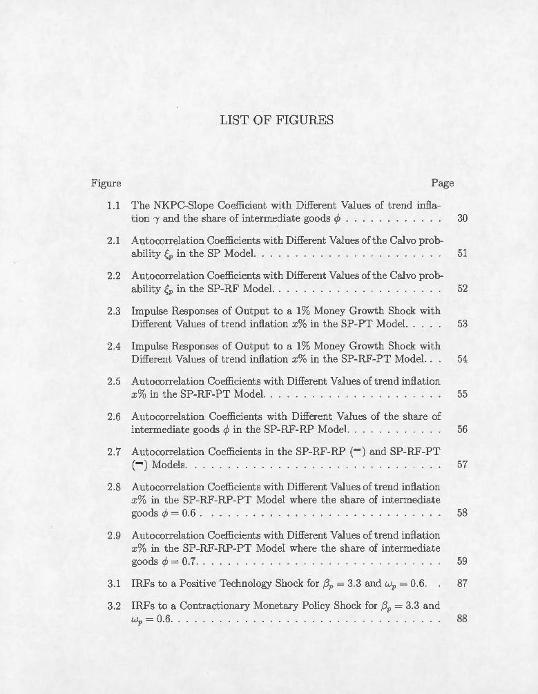
LIST OF FIGURES

Figure Page

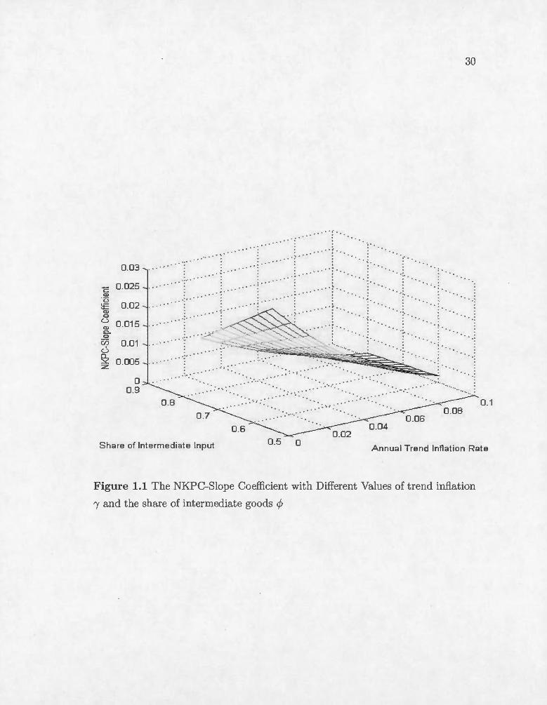
1.1 The NKPC-Slope Coefficient with Different Values of trend infla-tion 1 and the share of intermediate goods cp . . . . . . . . . . . . 30

2.1 Autocorrelation Coefficients with Different Values of the Calvo prob-ability Çp in the SP Model. . . . . . . . . . . . . . . . . . . . . . . 51

2.2 Autocorrelation Coefficients with Different Values of the Calvo prob-ability Çp in the SP-RF Model. . . . . . . . . . . . . . . . . . . . . 52

2.3 Impulse Responses of Output to a 1% Money Growth Shock with Different Values of trend inflation x% in t he SP-PT Model. . . . . 53

2.4 Impulse Responses of Output to a 1% :t-.1oney Growth Shock with Different Values of trend inflation x% in the SP-RF-PT Model. . . 54

2.5 Autocorrelation Coefficients with Different Values of trend inflation x% in the SP-RF-PT Model. . . . . . . . . . . . . . . . . . . . . . 55

2.6 Autocorrelation Coefficients with Different Values of the share of intermediate goods cp in the SP-RF-RP Model. . . . . . . . . . . . 56

2.7 Autocorrelation Coefficients in the SP-RF-RP (- ) and SP-RF-PT (- ) Models. . . . . . . . . . . . . . . . . . . . . . . . . . . . . . . 57

2.8 Autocorrelation Coefficients with Different Values of trend inflation x% in the SP-RF-RP-PT Model where the share of intermediate goods cp = 0.6 . . . . . . . . . . . . . . . . . . . . . . . . . . . . . 58

2.9 Autocorrelation Coefficients with Different Values of trend inflation x% in the SP-RF-RP-PT Model where the share of intermediate goods cp = 0.7. . . . . . . . . . . . . . . . . . . . . . . . . . . . . 59

3.1 IRFs to a Positive Technology Shock for {Jp = 3.3 and wP = 0.6 . 87

3.2 IRFs to a Contractionary Monetary Policy Shock for {Jp = 3.3 and Wp = 0.6. . . . . . . . . . . . . . . . . . . . . . . . . . . . . . . . . 88

lX

303 IRFs to a Positive Financial Market Shock for {3p > 1 and wp = 006 0 89

304 IRFs to a Posit ive Financial Market Shock for {3p = 303, {3p = 505 and wP = 0060 0 0 0 0 0 0 0 0 0 0 0 0 0 0 0 0 0 0 0 0 0 0 0 0 0 0 0 0 0 90

305 IRFs to a Positive Financial Market Shock for wP = 006, wP = 004 and {3p = 3030 0 0 0 0 0 0 0 0 0 0 0 0 0 0 0 0 0 0 0 0 0 0 0 0 0 0 0 0 0 91

306 IRFs to a Posit ive Financial Market Shock for {3P < 0 and wP = 0060 92

- ------- -- - -- ---------------------------

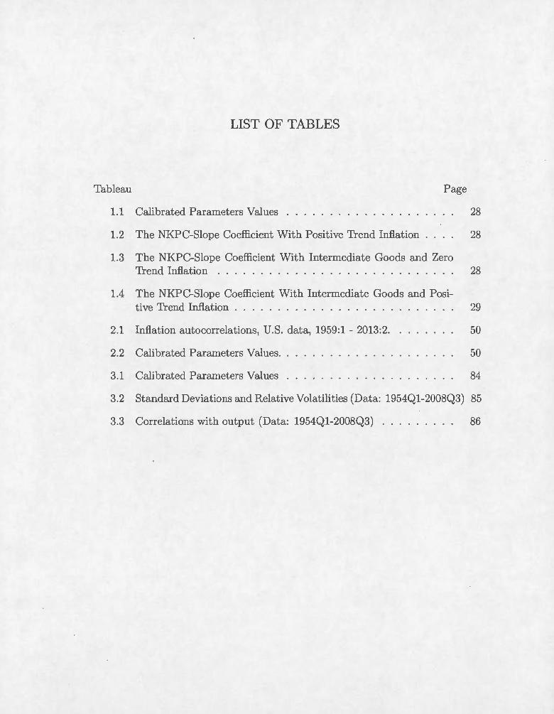
LIST OF TABLES

Tableau Page

1.1 Calibrated Para.meters Values 28

1.2 The NKPC-Slope Coefficient With Positive Trend Inflation 28

1.3 The NKPC-Slope Coefficient With Intermediate Goods and Zero Trend Inflation . . . . . . . . . . . . . . . . . . . . . . . . . . . . 28

1.4 The NKPC-Slope Coefficient With Intermediate Goods and Posi-tive Trend Inflation . . . . . . . . . . . . . . . . . . . 29

2.1 Inflation autocorrelations, U.S. data, 1959:1 - 2013:2. 50

2.2 Calibrated Parameters Values. 50

3.1 Calibrated Parameters Values 84

3.2 Standard Deviations and Relative Volatilities (Data: 1954Q1-2008Q3) 85

3.3 Correlations with output (Data: 1954Q1-2008Q3) . . . . . . . . . 86

RÉSUMÉ

Cette thèse comprend trois chapitres relatifs aux dynamiques à court t erme de l'inflation et à l'impact des marchés financiers sur l'économie réelle.

Le premier chapitre propose un modèle d 'équilibre général dynamique et stochastique (DSG E) qui incorpore une structure en boucle de production à côté du t rend d 'inflation positif, afin d 'analyser les sources des dynamiques à court terme de l'inflation. Il s 'agit principalement de développer pour la première fois dans la lit térature et en présence de ces deux ingrédients, une formulation générale de la courbe de Phillips néo-keynésienne où, l'inflation est exprimée comme une fonction des coûts marginaux réels et de l'inflation future ant icipée. En se concen­trant sur l'analyse de la pente de la courbe de Phillips, nous montrons que le trend d 'inflation positif et la structure en boucle de production sont nécessaires pour expliquer la persistance de 1 'inflation observée dans les données. Cependant , sous des valeurs raisonnables du trend d 'inflation, les inputs intermédiaires jouent un rôle beaucoup plus important que le trend d 'inflation en ce qui concerne la persistance inflationniste.

Dans le deuxième chapitre, nous visons à approfondir notre compréhension des dynamiques à court terme de l'inflation. Pour ce faire, nous simulons un modèle DSGE qui intègre non seulement la structure en boucle de production et le t rend d'inflation positif, mais aussi des frictions réelles comme la formation d 'habitude de consommation, les coûts d 'ajustement du capital et l'utilisation variable du ca­pital. Les autocorrélations théoriques de l 'inflation obtenues du modèle simulé sont ensuite confrontées à celles observées dans les données de 1 économie américaine. Les conclusions de la démarche analytique du premier chapitre sont confirmées ici. En effet , nous trouvons d 'une part que le trend d 'inflation positif a un effet négligeable sur la persistance de l'inflation en présence des inputs intermédiaires. D'autre part , la structure en boucle de production fournit une meilleure explica­t ion de l'évidence empirique sur la persistance de l'inflation.

Le troisième chapitre étudie les interconnections entre les marchés financiers et l'économie réelle. Le cadre d 'analyse est un modèle DSGE qui rend compte des interventions des ménages sur les marchés financiers, à travers le modèle d'évaluation des actifs financiers de Fama et French (2004) . Par ailleurs, nous proposons une modélisation explicite des dynan1iques des marchés financiers sur

Xll

la base du mouvement brownien géométrique. Comme résultats, nous mont rons que la consommation, l'output et l'investissement réagissent moins alors que l'in­flation et le travail réagissent plus fortement au choc technologique ici, que dans le cas d 'une économie où le secteur financier est ignoré. En outre, les effets négatifs d 'un choc de politique monétaire restrictive sur l'output, la consmrunation, l 'in­flation, l'investissement et le t ravail sont beaucoup plus importants. Par ailleurs, nous t rouvons qu'un choc posit if aux marchés financiers exerce une pression à la baisse sur le taux œintérêt nominal lorsque le coefficient beta du portefeuille d 'actifs du ménage est positif. Enfin , le modèle DSGE avec le secteur financier reproduit mieux la plupart des caractéristiques de l'économe U.S. , en part iculier, les volatilités et autocorrélations des principales variables macroéconomiques ainsi que leurs corrélations avec l'output .

Mots-clés : Dynamiques de 1 inflation, persistance de l 'inflation, prix ri­gides, biens intermédiaires, t rend d 'inflation positif, production en boucle, CAPM, marchés boursiers, politique monétaire, choix de portefeuille, mouvement brow­nien géométrique.

ABSTRACT

This thesis consists of three chapters related to short-term dynamics of inflation and the impact of financial markets on the real economy.

The first chapter offers a dynamic stochastic general equilibrium (DSGE) model that incorporates a roundabout structure of production alongside a positive inflation trend, to analyze the sources of short-term dynamics of inflation. In presence of both ingredients, the main goal here is to develop for the first time in the li terature, a general New Keynesiru1 Phillips Curve (NKPC) formulation , where inflation is expressed as a function of real marginal costs and expected future inflation. Focusing in our ru1alysis on the NKPC-slope coefficient, we show that both ingredients are necessary to account for inflation persistence observed in the data. However, under plausible values of trend inflation, intermediate goods play a more significant role shaping inflation persistence thru1 trend inflation.

In the second chapter, we aim to deepen our understanding of short-term dynamics of inflation. To do so, we simulate a DSGE model that incorporates not only roundabout production and positive trend inflation, but also real frictions such as habit formation, capital adjustment costs and variable capital utilization. The theoretical autocorrelations of inflation obtained from the simulated model are then compared with those observed in the U.S. data. The findings of the analytical approach of the first chapter are confirmed here. In fact , we find first that the positive trend inflation appears to have a negligible impact on inflation persistence when allowing for roundabout production. Second, intermediate goods provide a better explru1ation of the empirical evidence on inflation persistence.

The third chapter explores the interconnections between financial markets and the real economy. The framework is a DSGE model that accounts for house­holds interventions on financial markets , through the capital asset pricing model (CAPM) of Fama and French (2004). Moreover, we propose an explicit modelling of financial markets dynamics based on geometrie brownian motion. As results, we show that consumption, output and investment react less to a technology shock, while the nominal interest rate, inflation and labor are responding more strongly, compared to the case where financial markets are ignored. Moreover , the negative effects of a tightening monetary policy shock on output, consumpt ion, inflation, investment and labor are more significant. Vve also find that a positive

XlV

financial markets shock exerts a downward pressure on the nominal interest rate when the beta coefficient of the assets portfolio is positive. Finally, we find that our model with a financial market sector is successful in reproducing most of the salient features of the U .S. economy, particularly, key macroeconomie volatilities, autocorrelations, and correlations with output.

Keywords: Inflation dynamics, inflation persistence, sticky priees , inter­mediate goods, positive trend inflation, roundabout production , CAPî-.ii , stock markets, monetary policy, portfolio choice, geometrie brownian motion.

INTRODUCTION

Le principal défi auquel s'attaque notre thèse est d aider non seulement

à une meilleure mise en application de la politique monétaire, mais aussi, à un

examen beaucoup plus approfondi des effets de cette dernière sur l'économie réelle.

Cela passe par deux canaux de recherche. D'abord, un objectif de maîtrise des

dynamiques à court terme de l 'inflation par les banques centrales et les chercheurs,

ce à quoi s'attèlent les deux premiers chapitres. Puis, une grande compréhension

par la communauté scientifique de l'analyse des interconnections entre les marchés

financiers et l'économie réelle que constitue l'objet du dernier chapitre.

Une relation structurelle clé dans la catégorie des modèles d 'équilibre général

dynamique et stochastique (DSGE) est la courbe de Phillips néo-keynésienne

(NKPC). La NKPC a connu ces dernières années, plusieurs développements visant

à mieux expliquer les dynamiques à court terme de 1 'inflation et à améliorer de

manière générale notre compréhension de la politique monétaire. La NKPC stan­

dard est log-linéarisée autour d'un trend d 'inflation nul. Cette hypothèse est d 'une

part, contrefactuelle à cause d 'un taux d 'inflation en moyenne positif enregistré

par les économies industrialisées de l'après-guerre, et d 'autre part, non anodine

comme tente de démontrer un courant de littérature récent. Ascru·i (2004) par

exemple, montre que le trend d 'inflation positif pourrait affecter de manière signi­

ficative les propriétés de court terme et de long terme des modèles à prix rigides,

alors que Ascari et Ropele (2007) et Coibion et Gorodnichenko (2011) trouvent

que même un trend d'inflation faible aurait un impact sur la politique monétaire

optimale et les dynamiques des variables macroéconomiques.

Cette thèse explore entre autres, et ce, à travers les deux premiers chapitres,

la NKPC et les sources des dynamiques de l'inflation dans une économie avec

trend d 'inflation positif. Mais pour la première fois dans ce type de littérature,

-------------

2

nous traitons cette problématique en utilisant un modèle DSGE qui incorpore non

seulement le trend d 'inflation positif, mais aussi et surtout une structure en boucle

de production. La prise en compte de la structure en boucle de production est

mot ivée par le fait que les biens finaux sont devenus de plus en plus sophistiqués

et complexes en t ermes de production, notamment de la période de l'ent re-deux

guerres à la période de l'après-guerre (voir , Basu et Taylor , 1999a, 1999b; Ranes,

1996, 1999; Huang, Liu et Phaneuf, 2004). Au début du dix-neuvième siècle, le

panier de consommation du ménage était principalement composé de biens rela­

t ivement non finis. Depuis lors, les économies industrialisées ont été caractérisées

par une augmentation des relations inputs-outputs dans la production des types

de biens entrant dans le panier de consommation finale. Huang, Liu et Phaneuf

(2004) mont rent que la part U.S. des inputs intermédiaires a augmenté de 0.3

- 0.4 durant la période de l'entre-deux guerres à 0.6 - 0.7 durant la période de

l'après-guerre, tandis que diverses études estiment que cette part se situe entre

0.6 et 0.9 pour la période de l' après-guerre (voir, Basu, 1995; Bergin et Feenstra ,

2000; Huang et Liu, 2001 ; Huang, Liu et Phaneuf, 2004; Naka.mura et Steinsson,

2010).

Ainsi, le premier chapitre propose pour la première fois dans ce type de

modèles DSGE, et en présence de la boucle de producton et du t rend posit if, une

formulation générale de la KPC où l'inflation est exprimée comme une fonction

des coüts marginaux réels et de l'inflation future ant icipée. Nous t rouvons ici

que les interactions entre les prix rigides, les inputs intermédiaires et le t rend

d'inflation posit if ont une forte influence sur la sensibilité de l'inflation aux coüts

marginaux réels. Toutefois, les biens intermédiaires semblent avoir un impact plus

important sur le coefficient de la pente de la KPC que le trend d 'inflation positif

suggéré par Ascari ( 2004).

Dans le même ordre d'idées, le deuxième chapitre est une extension du

modèle DSGE à trend d 'inflation posit if de Ascari (2004). Nous bonifions ce

modèle en intégrant non seulement la structure en boucle de production , mais

aussi diverses frictions réelles comme la formation d 'habit ude de consommation,

les coûts d 'ajustement du capital et l'ut ilisation variable du capitaL Ces fric-

3

tions réelles standard dans la littérature DSGE, semblent incontournables dès

lors qu'on veut analyser la persistance des variables macroéconomiques (CEE,

2005; Smets and vVouters, 2003). La démarche ici, consiste d'abord à générer les

autocorrélations de l'inflation à partir du modèle simulé, et ensuite, à les comparer

à celles observées dans les données de 1 économie américaine. Il s'en suit que le

trend d'inflation positif a un effet négligeable sur les dynamiques de l'inflation

en présence des inputs intermédiaires, et que ces derniers donnent une meilleure

explication de l'évidence empirique sur la persistance de l'inflation. Ces résultats

confortent ainsi nos conclusions de la démarche analytique du premier chapitre.

Enfin le troisième chapitre s'inscrit dans la deuxième problématique de

notre thèse, à savoir, les interconnections entres les marchés financiers et l'économie

réelle. Le point de départ de ce travail est la récente crise financière de 2008,

qui a montré comment des chocs négatifs aux marchés financiers pouvaient se

transformer en des conséquences néfastes pour l'économie réelle. Cette crise a

aussi mis en évidence l'inefficacité des instruments traditionnels de la politique

monétaire dans un contexte de taux d 'intérêt proches de la borne zéro. D 'oü, la

nécessité d 'un plus grand intérêt pour les marchés financiers ainsi qu 'une anal­

yse plus poussée de leurs impacts sur l'économie réelle. Nous nous attelons à

cela en proposant un cadre d 'analyse DSGE qui intègre le modèle d 'évaluation

des actifs financiers, pour rendre compte des interventions des ménages sur les

marchés financiers (voir, Markm;<,ritz, 1959; Sharpe, 1964; Lintner, 1965; Fama,

1996; et Fama et French, 2004). Le modèle d'évaluation des actifs financiers sup­

pose que les individus détiennent un portefeuille d'actifs composé d 'actifs sans

risque, et d'actifs risqués disponibles sur les marchés boursiers. De plus, une

modélisation explicite des dynamiques des marchés financiers est proposée en se

basant sur le mouvement brownien géométrique (voir, Kendall et Hill , 1953; Os­

borne, 1959; Roberts, 1959; Samuelson, 1965; Black et Scholes, 1973; Barmish et

Primbs, 2011; et Lochowski et Thagunna, 2013). Nos résultats suggèrent que la

consommation, l'output et l'investissement réagissent moins, alors que l 'inflation

et le travail réagissent plus fortement au choc technologique ici, que dans le cas

d'une économie oü le secteur financier est ignoré. Aussi, les effets négatifs d'un

4

choc de politique monétaire restrictive sur l'output , la consommation, l'inflation,

l'investissement et le travail sont beaucoup plus importants. Par ailleurs, nous

trouvons qu 'un choc positif aux marchés financiers exerce une pression à la baisse

sur le taux d 'intérêt nominal lorsque le coefficient beta du portefeuille d 'actifs

du ménage est positif. Enfin, le modèle DSGE avec le secteur financier repro­

duit mieux la plupart des caractéristiques de l'économe U.S. , en particulier, les

volatilités et autocorrélations des principales variables macroéconomiques ainsi

que leurs corrélations avec l'output . Par conséquent, les marchés financiers, et

plus précisément les marchés boursiers mériteraient une attention particulière de

la part des autorités monétaires et des chercheurs , lorsqu 'on vise à mieux com­

prendre les tenants et aboutissants de la politique monétaire.

CHAPTER I

THE NEW KEYNESIAN PHILLIPS CURVE: INTERMEDIATE GOODS MEET POSITIVE TREND INFLATION

Abstract

What happens when intermediate goods meet positive trend inflation in a ew

Keynesian Phillips Cmve (NKPC) madel? Focusing on the slope coefficient on marginal

cost, our analysis shows the effects are dramatic. Unlike the basic Calvo price-setting

madel which requires an extremely law frequency of priee adjustment or backward­

looking components to account for inflation persistence, om madel with sticky priees,

roundabout production and trend inflation does successfully so with a plausible fre­

quency of priee changes, and realistic values of trend inflation and share of intermediate

inputs. While trend inflation plays a non negligible role in explaining inflation dynamics,

accounting for roundabout production seems to be more important .

JEL classification: E31 , E32.

Keywords: Inflation dynamics; sticky priees; intermediate goods; trend inflat ion.

6

1.1 Introduction

A key st ructural relationship in a large class of dynamic stochastic gen­

eral equilibrium (DSGE) models is the so-callcd New Keynesian Phillips curve

( KPC) . The NKPC has undergone sever al developments in recent years aimed

at better tracking short-run inflation dynamics and improving our understanding

of monetary policy more generally. The standard NKPC is log-linearizcd around

a zero steady-st ate rat e of inflation. This assumption is not only counterfactual

since postwar industrialized economies have experienced positive inflat ion on aver­

age, it is not innocuous as a recent body of research tends to demonstrate. Ascari

(2004), for instance, shows that positive trend inflation may significantly alter the

short-run and long-run properties of sticky-price models, while Ascari and Ropele

(2007) and Coibion and Gorodnichenko (2011) argue that even low trend inflation

may affect optimal monetary policy and the dynamics of macro variables.

The present paper further explores the KPC and the sources of inflation

dynamics in an economy with positive trend inflation. But for the first time

in this type of literature, wc address this quest ion using a DSGE framework in

which intermediat e goods meet posit ive trend inflation. Focusing in our analysis

on the dynamic response of inflation to real marginal costs (G alf and Gertler ,

1999; Ascari 2004), t o which we refer throughout the paper as slope coefficient

on marginal cast or NKPC-slope coefficient , we show that both ingredients are

necessary to account for the observed inertial behavior of inflation, but that under

plausible values of trend inflation, intermediate goods play a more significant role

shaping inflation dynamics than trend inflation.

A well known property of t he basic new keynesian sticky-price model with

zero trend inflation is that the NKPC is purely forward-looking in that current

inflation depends on current real marginal costs and expected future inflation.

As we discuss in Section 2 of the paper , the basic KPC is hardly reconcilable

with the inertial behavior of inflation unless assuming an implausibly long aver­

age waiting time between priee adjustments, backward-looking components (Gal!

and Gertler, 1999; Christiano, Eichenbaum and Evans, 2005; Smets and Vlouters,

7

2007; Justiniano and Primiceri, 2008), or slow-moving (random walk) trend infla­

t ion (Cogley and Sbordone, 2008).

Here, we combine a roundabout production structure with non-zero steady­

state inflat ion in Calvo's (1983) price-setting framework. Previous research has

established that in arder to generate a high posit ive serial correlation of inflation

as observed in the U.S. data, the basic KPC requires assuming a very high prob­

ability of priee non-reopt imization. Vlorking from the Calvo sticky-price madel

of King and ·w atson (1996) , Nelson (1998, Table 3) shows that this probability

must be close to 0.9 to match inflation persistence. This in t urn implies an average

wait ing time between priee adjustments of 2.5 years or more, which clearly is coun­

terfactual. With a subjective discount factor of 0.99, the NKPC-slope coefficient

would have to be 0.012 more or less. If the probability of priee non-reopt imization

is set instead at t he more convent ional value of O. 75, the NKPC-slope coefficient

increases to 0.086, which is 7 times larger than required to match inflation inertia.

The inability of the basic NKPC model t o account for inflation persistence

without assuming an implausibly low frequency of priee adjustments has led re­

searchers to incorporate mechanisms like rule-of-t humb behavior of priee-setters,

backward indexation of priees, and slow-moving trend inflation in new keynesian

pricing models (Galf and Gertler , 1999; Christiano, Eichenbaum and Evans, 2005;

Smets and ~Touters, 2007; Justiniano and Primiceri , 2008; Cogley and Sbordone,

2008).

Cont rasting sharply wit h previous studies, our approach does not need to

rely on such ingredients to be consistent with inflation persistence. St ill , it is fully .

consistent with the optimizing behavior of households and firms. Our framework is

one that exploits strong interactions between a roundabout production structure,

sticky priees and positive trend inflation. Our use of a roundabout production

structure is motivated by the fact that final goods have become more processed

and increasingly sophisticated over time, especially from the interwar period to the

postwar period (e.g., Basu and Taylor, 1999a, 1999b; Ranes, 1996, 1999; Huang,

Liu and Phaneuf, 2004). In the early Twent ieth Cent ury, a household 's consump-

8

tion basket was primarily composed of relatively unfinished goods. Since then,

industrialized economies have been characterized by increased roundaboutness in

the production of typical goods entering the final consumption basket . 1 Huang,

Liu and Phaneuf (2004) document that the U.S. share of intermediate inputs has

risen from 0.3- 0.4 during the interwar period to 0.6 - 0.7 during the postwar

period , _wherea..s a variety of studies evaluate that this share lies between 0.6 and

0.9 for the postwar period. 2

Working from a state-dependent model with nominal priee rigidi ty, Basu

(1995) shows t hat eombining input-output linkages between firms with small

(menu) eost of ehanging priees ean give rise to a multiplier for priee stiekiness

(IviPS): beeause all firms in the eeonomy face sticky priees and use intermediat e

inputs, firms ' prieing decisions beeome intereonneeted, so that the an1ount of priee

stiekiness at the aggregate level may well exceed that observed at t he individual

firm level. Using a fully artieulat ed DSGE model with nominal and real frictions,

El Omari and Phaneuf (2011) provide quanti tative evidence that the MPS may

be an important source of inflation inertia and persistenee in aggregate quantit ies

in a Calvo wage-and-price-setting framework with zero steady-state inflation.

Aseari (2004) extends the standard new keynesian prieing model to aeeount

for posit ive t rend inflation, showing that positive steady-state inflation ean sig­

nifieantly flat ten the NKPC while redueing the sensitivity of eurrent inflation to

the eurrent output gap. For example, assuming an annualized trend inflation of

1. Ranes (1996) reports that the share of crude material inputs in final U.S . output has

decreased from 26% to. only 6% from the early twent ieth century t o the end of the 1960's.

Furthermore , based on the household budget surveys, he reports that the share of consumption

expendi tures on food (excluding restaurant meals) has declined from 44% at t he t urn of the

Twentieth Century to 11.3% in 1986, while the share of the budget ca.tegory "Other" including

many complex goods such as automobiles has risen steadily from 17% to 45.8% during t he scune

period.

2. Basu (1995) argues that t his share can be as high as 0.8, Bergin and Feenstra (2000)

assume that it lies between 0.8 and 0.9, wherea.s Huang and Liu (2001) , Huang, Liu and Phaneuf

(2004) and Nakamura and Steinsson (2010) assume a, share of intennediate inputs of 0.7.

9

only 2% and an elasticity of substitution between differentiated goods of 10, he

shows that the slope coefficient on marginal cost decreases by 30% relatively to

the basic madel with zero-trend inflation. With a 5% trend inflation, the KPC­

slope coefficient drops by 64%. However, trend inflation must reach 8% to bring

the KPC-slope coefficient down to 0.012. Such a high steady-state rate of infla­

tion seems implausible since the U.S. economy has experienced an average rate of

inflation of 3.57% over the years 1960-2011 , and 5% during the 1960s and 1970s,

a time of high inflation.

Vve develop a general NKPC formulation that encompasses four different

models: i) the basic price-setting madel with zero-trend inflation, ii) a madel with

sticky priees, positive trend inflation and no input-output linkages , iii) a madel

with sticky priees, zero-trend inflation and intermediate inputs, and finally, iv)

a madel with sticky priees, positive trend inflation and intermediate inputs. We

show that in all four models , inflation is expressed as a function of real marginal

costs and expected future inflation, with a slope coefficient which is analytically

and quantitatively different among the four models.

\T'le provide evidence showing that the interactions between intermediate

inputs, sticky pdces and positive trend inflation exert a powerful impact on the

response of inflation to real marginal costs. For instance, for a median waiting

time between priee adjustments of 7.2 months, broadly consistent with micro-level

evidence on the behavior of priees (Bils and Klenow, 2004; N akamura and Steins­

son, 2008) , we find that an annualized steady-state rate of inflation of only 1%,

combined with a share of intermediate inputs of 0.6, reduce the slope coefficient

on marginal cost to 0.029, which is nearly 66% lower than in the basic model with

zero-trend inflation and no intermediate inputs. This reduction reaches 81% when

trend inflation is 4%. But more importantly, with a rate of trend inflation between

3 to 5% and a share of intermediate inputs between 0.6 and 0.8, the NKPC-slope

coefficient is always small, ranging from 0.006 to 0.02 , which is broadly consistent

with observed inflation dynamics.

However, among these two factors , intermediate inputs seem to have a larger

10

impact on the IKPC-slope coefficient than positive trend inflation. That is, as­

suming a share of intermediate inputs of 0.6 in a madel with sticky priees and

zero steady-state inflation lowers the slope coefficient by roughly 60% relative

to the basic madel. Renee, the MPS is by itself an important channel of in­

flation persistence. However, we also show that with zero trend inflation, the

share of intermediate inputs must be 0.8 or higher to bring the slope coefficient

down to 0.012. Thus, while playing a smaller role than the MPS in reducing the

NKPC-slope coefficient, taking into account positive trend inflation is nonetheless

important to explain inflation dynamics. Furthermore, even when the frequency

of priee adjustments is set at a higher pace we find that intermediate inputs and

positive trend inflation have a powerful impact on the NKPC.

The rest of the paper is organized as follows. Section 2 traces back the var- ·

ious incarnations the NKPC has taken over the years, while giving some perspec­

tive on other approaches 'vhich have been followed to study inflation dynamics.

Section 3 describes our DSGE madel with sticky priees, roundabout production

and positive trend inflation. Section 4 derives our general KPC formulation

and compares NKPC-slope coefficients in alternative models. Section 5 discusses

calibration issues and presents our main findings. Section 6 offers concluding

remarks.

1.2 The Various Incarnations of the NKPC

This section succintly analyzes the several incarnations the NKPC has gone

through during the last fifteen years or so. 3

3. Vve purpo efully restrict our analysis to new keynesian models involving nominal priee

stickiness.

11

1.2.1 The Forward-Looking NKPC

The standard Calvo sticky-price formulation implies a NKPC of the fonn:

(1.1)

where 1rt indicates the inflation rate , mCt; denotes the firm 's real marginal cost,

and the slope coefficient on marginal cost, À= (1- ~p)(1- (3~p)/f,p , depends on

the probability of priee non-reoptimization f,p and the subjective discount factor

(3 . Because the KPC (1.1) is forward-looking, the Calvo price-setting model

must rely on a high probability of priee non reoptimization ~P (resulting in a low

..\) to account for inflation persistence. Nelson (1998) shows that the standard

Calvo sticky-price model generates high serial correlations of inflation as observed

in the U.S. data with f,p = 0.9, implying an average waiting time between priee

adjustments of 2.5 years. This is implausibly long in light of microeconomie

evidence on U.S. priee behavior suggesting a median waiting time between 4.3

and 9 months for priee changes (Bils and Klenow, 2004; Nakamura and Steinsson,

2008).

A subsequent development by \iVoodford (2003, ch.3 ; 2005) incorporates

firm-specific (immobile) capital and variable demand elasticity into the otherwise

standard Calvo sticky-price model. The marginal cost of the optimizing firm then

differs from aggregate marginal cost by a function of its relative priee. Denoting

the elasticity of substitution among differentiated goods by e, and the elasticity

of marginal cost to firms ' output by x, the NKPC becomes:

1rt = ÀcmCt + f3 Et { 7rt+l} , (1.2)

where Àc = (1- f,p)(l- (3f,p)f~p(l +ex). This formulation accommodates a lower

slope coefficient on marginal cost for a given value of ~v· That is, the higher ex, the lower Àc, and the weaker is the response of inflation to real marginal cost.

Therefore, the probability of priee non-reoptimization does not have to be as high

as in the basic model to account for inertial inflation. 4

4. See Eichenba.um and Fisher (2007) for an empirical investigation of the Calvo pricing

model with firm-specific capital.

12

1.2.2 Backward-Looking Elements and the NKPC

One important development , initiated by the work of Cali and Certler

(1999) , is the addition of backward-looking components to the NKPC intended

to capture the inertial behavior of inflation. Calî and Certler propose a variant

of the Calvo pricing model in which firms facing the signal 1 - f,p authorizing

priee changes are divided in two groups. One group of firms, in proportion w, sets

priees equal to the average priee in the most recent round of priee adjustment,

plus a correction for last period rate of inflation. The other group, in proportion

( 1 - w) , sets priees optimally as in the basic, forward-looking priee-set t ing mo del.

This refinement leads to the following hybrid NKPC:

(1.3)

where Àh = (1- w)(1- Çp)(1- (3 f,p) r.p-l, '"Yi = (3 f,p r.p-l, '"Yb- wr.p-1 and r.p = Çp + w [1- Çp(1- (3)]. The presence of rule-of-thumbers has three main consequences:

it adds previous period inflation to the NKPC, lowers the slope coefficient on

marginal cost and reduces the impact of expected future inflat ion on current

inflation. Cali and Certler (1999) report estimates suggest ing that the backward­

looking tenu in (1.3) is statistically significant and relatively modest, helping the

hybrid formulation to better capture inflation dynamics.

In the same vein, Christiane, Eichenbaum and Evans (2005) propose a setup

where firms which are not allowed to reoptimize their priee in a given period will

nonetheless index them to last period inflation. The remaining firms reset priees

optimally as in the standard model. 5 The resulting NKPC is similar to (1.3),

except that the coefficient on previous period inflation depends upon the degree

of backward indexation. CEE argue that backward indexation helps reproduce the

impulse responses of inflation and output to a monetary policy shock estimated

from a structural vector autoregression.

The use of backward-looking terms has been subject to criticism. Woodford

5. More precisely, in CEE's mode!, both households and firms not a uthorized to reoptimize

their wages and priees, respective! y, in a given period v..ill index them to last past period inflation.

---------

13

(2007), Cogley and Sbordone (2008) and Chari, Kehoe and McGrattan (2009) note

that rule-of-thumb behavior of priee-setters and backward indexation both lad:

a convincing microeconomie justification and are therefore ad hoc mechanisms.

Moreover, both mechanism .. CJ have unattractive empirical implications. Vvhile the

estimates reported in Galf and Gertler (1999) suggest that rule-of-thumb behav­

ior is modest , the frequency of priee adjustments implied by the hybrid model

romains low and far from micro level evidence. Backward indexation, on the

other hand, implies that all firms change their priees once every three months,

which is counterfactual.

1.2.3 Trend Inflation and the NKPC

While the above relationships are derived for a log-linearization around

zero-trend inflation, a recent strand of literature imposes log-linearizing the non­

linear equilibrium conditions of the Calvo model around a steady state with a

time-varying trend inflation (Cogley and Sbordone, 2005, 2008; Ireland, 2007).

This refinement leads to the following NKPC: 00

Kt= Àtviiîct + altEt {Kt+I} + a2t L ~{;1 Et {Kt+j}. j = 2

(1.4)

Here the symbol - over a variable denotes a log-deviation from trend value, and

hence mCt = mCt -mCt and Kt= 1ït -1ft , where mCt and 'ift are trend variables, and

Àtv , alt and a2t are time-varying parameters evolving with trend inflation. Fur­

thermore, Cogley and Sbordone (2008) assume strategie complementarity, so these

parameters also depend on e and X· ote that Cogley and Sbordone's original

formulation is even more general than (1.4) , since it also embeds backward index­

ation. However , we omit the backward-looking component for the reasons above,

and because it is found to be statistically insignificant when time-vary!ng trend

inflation is also taken into account (see, Cogley and Sbordone, 2008). Cogley and

Sbordone model trend inflation as a driftless random-walk. Their estimates imply

a mean duration of priees which roughly consistent with the evidence reported in

Bils and Klenow (2004). Despite the merits of this approach, West (2007) ques­

tions the use of the random walk as a way of modeling trend inflation, arguing

14

that there is no economie rationale offered for this assumption. He therefore con­

eludes that (1.4), like the NKPC with backward-looking components, relies on

exogenous rather than intrinsic sources of inertia.

Ascari (2004) and Ascari and Ropele (2007) consider the ca..se of a constant,

nonzero steady-state rate of inflation in a purely forward-looking price-setting

model. Trend inflation is directly linked to monetary policy through the gross

steady-state growth rate of money supply denoted by 'Y· The NKPC with posit ive

trend inflation is:

where À(r) = c~;;t;1

) (1 - f,p/3r0) and F is a function of expected future infla­

t ion and output. With zero steady-state inflation, 'Y = 1, and (1.5) bolds down to

the basic KPC. The slope coefficient on marginal cost, À(r) , is nowa function of

positive trend inflation. Assuming [3 = 0.99 , e = 10 and Çp = 0.75, Ascari (2004)

shows that À ('Y) is sm aller t h an À by 30% with an annualized trend inflation rate

of 2%, by 64% \Nith 5% trend inflation and by 95% if trend inflation is 10%. Thus,

positive trend inflation may significantly affect inflation dynamics.

1.3 A NKPC Model with Intermediate Goods and Positive Trend

Inflation

Since our focus is on the KPC and the slope coefficient on marginal cost,

we follow Gall and Gertler (1999) and limit our modeling strategy to an envi­

ronment of monopolistically competitive :firms facing sticky priees. Our model

rests on three main pillars. First , the production structure reflects the reality

t hat many goods produced in industrialized economies have become increa..singly

processed over t ime (e.g., see Ba..su, 1995; Huang, Liu and Phaneuf, 2004) . We

model the increased sophistication of goods produced as a roundabout process,

where all firms use intermediate inputs in production. Basu (1995) endorses the ·

roundabout production structure based on the evidence from input-output stud­

ies showing that "even the most detailed input-output tables show surprisingly

15

few zeros" (p.514). Second, ·priees are sticky. As Basu suggests, when combined

with sticky priees, intermediate goods can act as a multiplier for priee stickiness

( ;IPS): a given amount of priee rigidity at the individual firm level may lead to

a higher degree of priee stickiness at the aggregate level. Third, following Ascari

(2004) and Ascari and Ropele (2007) , we assume positive trend inflation.

1.3.1 Optimal Pricing Decisions

Denote by Xt a composite of differentiated goods Xt(j) for j E [0, 1] such

that Xt = [!~ X t(j) (O-l) /O dj] 0f(B-l)) where e E (1 , 00) is the elasticity of substitu­

tion between the goods. The composite good is produced in a perfectly competi­

tive agg1·egate sector.

The demand function for good of t:n)e j resulting from optimizing behavior

in the aggregation sector is given by

(1.6)

where Pt is the priee of the composite good related to the priees Pt(j) for j E [0, 1]

of the differentiated goods by Pt = [f~ Pt(j)<1- 0ldj]l l( l-B).

The central feature of the madel is that the composite good can serve either

as a final consumption or investment good, or as an intermediate production input.

The production of good j requires the use of capital labor, and intermediate

inputs:

(1. 7)

where rt(j) is the input of intermediate goods, Kt(j) is the physical capital stock,

Lt(j) denotes total hours worked, and F is a fixed cost v.rhich is identical across

firms. The parameter cp E (0 , 1) measures the elasticity of output with respect to

intermediate input , and the parameters a E (0, 1) and (1 -a) are the elasticities

of value-added with respect to the capital and labor input , respectively.

Each firm acts as a price-taker in the input markets and as a monopolistic

competitor in the product market. A firm chooses the priee of its product, taking

16

the demand schedule in (1.6) as given. Priees are set according to the mechanism

spelled out in Calvo (1983). In each period, a firm faces a constant probability

1 - Çp of reoptimizing its priee, with the ability to reoptimize being independent

across firms and time.

A firm j allowed to reset its priee at date t chooses a priee Pt(j) that

maximizes its profits,

00

Et L(çpy-tDt,T[Pt(j)X~(j)- V(X~(j))], (1.8) T=t

where E is an expectations operator, Dt,T is the priee of a dollar at ti me T in

units of dollars at time t and V(X~(j)) is the cost of producing X~(j), equal to

VT[X~(j) + F], and ~ denotes the marginal cost of production at time T.

Solving the profit-maximization problem yields the following optimal pricing

decision rule:

lEt f (Çp)'"- t Dt ,TX~(j)VT ]

P,(j) = (e ~ 1) E: ~(Ç.)'-'D,,rXf(i) , (1.9)

which says the optimal priee is a constant markup over a weighted average of

marginal costs during the periods the priee will remain effective.

Solving the firm's cost minimization problem yields the following nominal

marginal cost function:

~ = 9P![(R~/~WT) 1-a]l-cf> , (1.10)

where R~ is the nominal rentai rate on capital, WT is the aggregate nominal wage

rate and "9 is a constant tenu determined by cp and a. The nominal marginal cost

records three components. Two of those are flexible , R~ and WT, ·while the other,

PT, is rigid since priees are sticky. The relative importance of the rigid priee PT

increa..ses with the share of intermediate inputs cp.

17

Real marginal cost is therefore expressed as:

(1.11)

with r~ = R~ / PT and wT = WT/ P,. . The higher the share of intermediate inputs </J,

the smaller the impact of the two flexible components r~ and wT on real marginal

cost . Thus, real marginal becomes increasingly sluggish as <P rises, enhancing

inflation persistence. With <P --+ 1, real marginal cost becomes almost insensitive

to variations in the real rental rate on capital and in the real wage.

In the standard Calvo price-setting model with no intermediate inputs ( <P = 0) , the real marginal cost is:

( k)a ( )1-a J\tfCsT = ~

1 ~Ta (1.12)

The conditional demand functions for the intermediate input and for the

primary factor inputs used in the production of X~(j) which are derived from

cost-minimization are r (:) = "' Vr[X~(j) + F]

T J l.f/ PT ' (1.13)

K ( .) = (1- "') VT[X~(j) + F] T J a '~' Rk '

T

(1.14)

and

(1.15)

A firm that does not reset its priee at a given date still has to choose the inputs

of the intermediate good, capital and labor to minimize production cost .

The pricing equation (3.4) can be rewritten as:

( e ) [Et ~(~py-t Dt,TMCrTP:Xrl

Pt(j) = -- __ T--~---------e- 1 E "'(t )T-tD p o-1x

t L.._.; '-, p t,T T T

T=t

(1.16)

From (l.ll) and (1.12) , we can establish the following log-linear relationship

between the real marginal cost with roundabout production and its counterpart

18

in the basic price-setting model:

(1.17)

In the absence of intermediate inputs (cp = 0) , t he real marginal cost is mer = mc87 , and

(1.18)

1.3.2 Monetary Policy

The government injects money into the economy through nominal transfers

so Tt = Mf - MZ_1 where M 5 is the aggregate nominal money supply. Further­

more following Ascari (2004) and Ascari and Ropele (2007), we assume that

steady-state mo ney supply evolves according to the fixed rule: JVft = ! iV!f_ 1 ,

where 1 is t he gross steady-state growth rate of nominal money supply and the

source of positive trend inflation.

1.3.3 Equilibrium and :rv.Iarket-Clearing Conditions

An equilibrium consists of allocations r t(j) , Kt(j) , Lt(j) and priee Pt(j)

for firm j , for all jE [0 , 1] together with priees Dt,t+1 , Pt, R~ , and ltlft , satisfying

the following conditions: (i) taking the nominal wage rate and all priees but its

own as given, each firm 's allocations and priee solve its maximization problem;

(ii) markets for bonds, capital, labor and the composite good clear; (iii) monetary

policy is as specified.

Along with (1.13), the market-clearing condition for the composite good

1

Yt + J r t(j )dj = xt , 0

implies that equilibrium real GDP is related to gross output by

vt rt = Xt - cp Pt [ GtXt + F] , (1.19)

where Gt- JJ[Pt(j)/Pt]-6dj captures the priee-dispersion effect ofstaggered priee

contracts .

19

Meanwhile, the market-clearing conditions J~ I<f(j)dj =Kt for capital and

J~ Lf(j)dj = Lf = L: for labor, along with (1.14) and (1. 15), imply that the

equilibrium aggregate capital stock and labor are related to gross output by

vt Kt-1 = a(1- cp) Rf [GtXt + F], (1.20)

(1.21)

Equations (1.19), (1.20) , and (1.21) , together with the price-setting equation (1.9)

characterize an equilibrium.

1.4 The NKPC: Intermediate Goods Nieet Positive Trend Infia-

ti on

Vve now examine how intermediate goods and positive trend inflation inter­

act to affect the NKPC. Our main focus is on the NKPC-slope coefficient or slope

coefficient on marginal cost .

1.4.1 Optimal Pricing Decisions with Intermediate Goods and

Non-Zero Trend Inflation

To see how intermediate goods and positive trend inflation affect the op­

timizing behavior of intermediate firms, we expand (1.16) and make explicit the

contribution of cumulative gross inflation rates (CGIR) to priee setting (e.g. see

Ascari and Ropele, 2007) 6 :

( ) [

Et ~--oot(~pt-tDt,rPfXr(ITt+l x Ilt+2 x .. . x IT7 )0MCrr ] .

Pt(j) = e ~ 1 , Et 2::: (Çp)T-t Dt,Tp:-1 Xr(ITt+1 x rrt+2 x ... x ITT )0- 1

T=t (1.22)

6. The CGIR between time t + 1 and T is rrt+l ,r = Ilt.+l x n t+2 x ... x liT) where

II,. = P,.fPr-1·

20

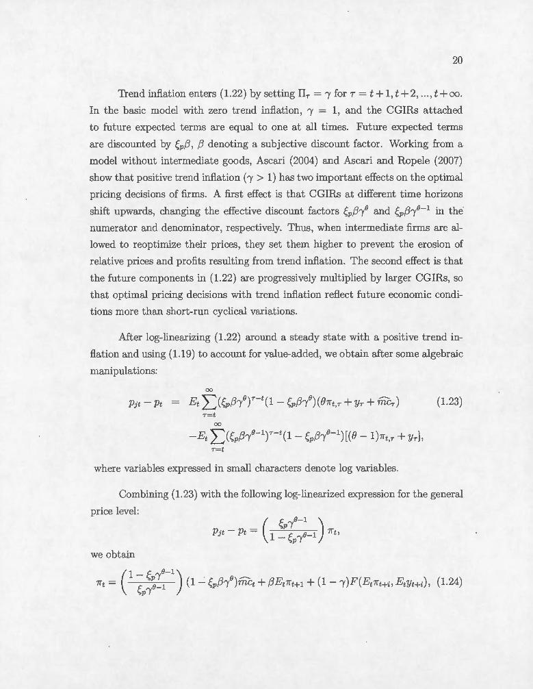
Trend inflation enters (1.22) by setting IIr = 1 for T = t + 1, t + 2, ... , t + oo.

In the basic madel with zero trend inflation, 1 = 1, and the CGIRs attached

to future expected tenns are equal to one at all times. Future expected tenns

are discounted by Çp/3, (3 denoting a subjective discount factor. Working from a

madel without intermediate goods, Ascari (2004) and Ascari and Ropele (2007)

show that positive trend inflation (! > 1) has two important effects on the optimal

pricing decisions of firms. A first effect is that CGIRs at different time horizons

shift upwards, changing the effective discount factors f,p /3/0 ru1d f,p /3/0- 1 in the·

numerator and denominator, respectively. Thus, when intermediate firms are al­

lowed to reoptimize their priees, they set them higher to prevent the erosion of

relative priees and profits resulting from trend inflation. The second effect is that

the future components in (1.22) are progressively multiplied by larger CGIRs, so

that optimal pricing decisions with trend inflation refiect fu ture economie condi­

tions more than short-run cyclical variations.

After log-linearizing (1.22) around a steady state with a positive trend in­

flation and using (1.19) to account for value-added, we obtain after some algebraic

mruüpulations:

00

Pjt- Pt Et ~(f,p/3!0r-t(1- f,p /3!0 )(B7rt,r + yT + mcT) (1.23) T=t

00

-Et ~(f,p/3/8-lr-t(1- Çp/3/0-

1)[(e- 1)7rt,T + Yr], T=t

where variables expressed in small characters denote log variables.

Combining (1.23) with the following log-linearized expression for the general

priee level:

we obtain

21

where

(1.25)

00

-(1- Çp{J--·-/-1 )Et 2::_)Çpf3r0-

1 yr-t[(B- 1)7rt+l,r+l + Yr+I]}. r=t

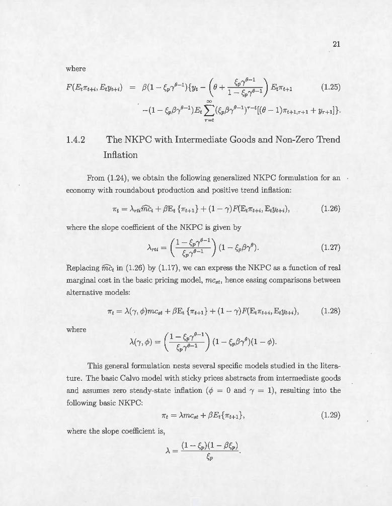
1.4.2 The NKPC with Intennediate Goods and Non-Zero Trend

Inflation

From (1.24), we obtain the following generalized I KPC formulation for an

economy with roundabout production and positive trend inflation:

(1.26)

where the slope coefficient of the NKPC is given by

(1- ~prO-l ) o

À rti = Çp10_1 (1- Çp fJI ). (1.27)

Replacing mCt in (1.26) by (1.17), we can express the KPC as a function of real

marginal cost in the basic pricing madel, mc5 t , hence easing comparisons between

alternative models:

(1.28)

where

This general formulation nests several specifie models studied in the litera­

ture. The basic Calvo madel with sticky priees abstracts from intermediate goods

and assumes zero steady-state inflation (cp = 0 and 1 = 1) , resul ting into t he

following basic NKPC:

(1.29)

where the slope coefficient is,

À= (1- ~p)(1 - fJÇp). Çp

22

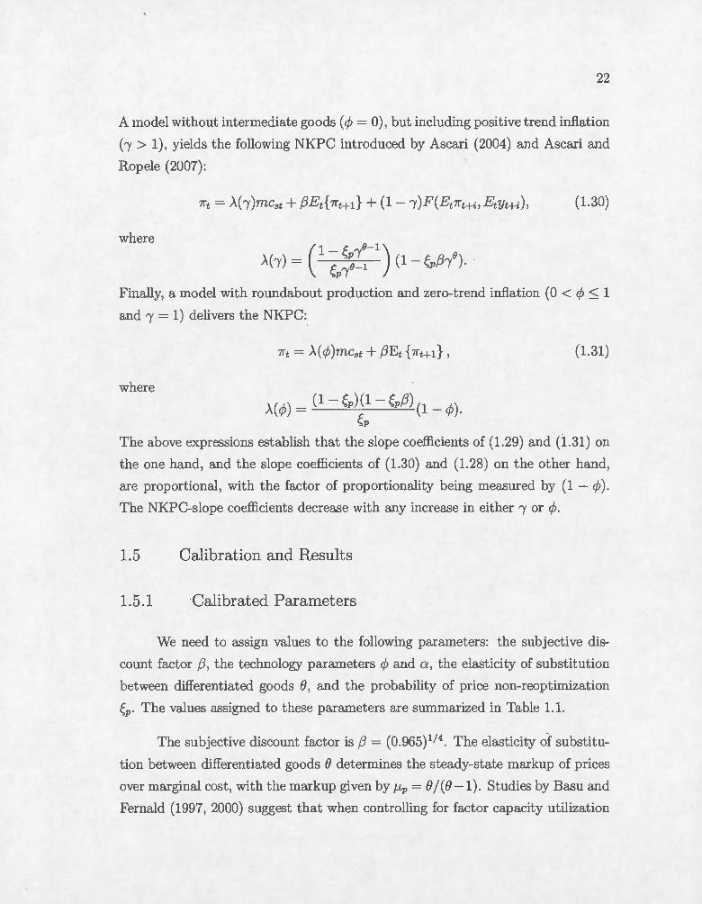
A mo del without intermediate goods (cp = 0) , but including positive trend inflation

(1 > 1) , yields the following NKPC introduced by Ascari (2004) and Ascari and

Ropele (2007):

(1.30)

where

(1 - Çp/8-1) 8

À(r ) = Çp/8-1 (1- Çp/3{ ).

Finally, a model with roundabout production and zero-trend inflation (0 < cp ~ 1

and 1 = 1) delivers the NKPC:

(1.31)

where À( cp) = (1- Çp)i: - Çp(3 ) (1- cp) .

The above expressions establish that the slope coefficients of (1.29) and (l.31) on

the one hand, and the slope coefficients of (1.30) and (1.28) on the other hand,

are proportional, with the factor of proportionality being mea..CJured by (1 - cp). The NKPC-slope coefficients decrease with any increase in either 1 or cp .

1.5 Calibration and Results

1.5.1 ·Calibrated Parameters

Vve need to assign values to the following parameters: t he subjective dis­

count factor (3, the technology parameters cp and a, the elasticity of substitution

between differentiated goods e, and the probability of priee non-reoptimization

Çp· The values assigned to these parameters are summarized in Table 1.1.

The subjective discount factor is f3 = (0.965) 114. The elasticity of substit u­

tion between differentiated goods e determines the steady-state markup of priees

over marginal cost , with the markup given by /.L p = e /(B -1). Studies by Basu and

Fernald (1997, 2000) suggest that when controlling for factor capacity utilization

23

rates , the value-added markup is about 1.05. \Vithout any utilization correc­

tion, the value-added markup would be more in the range of 1.12. Rotemberg

and vVoodford (1997) suggest a higher value-added markup of about 1.2 without

correcting for factor utilization. Since we do not focus on variations in factor uti­

lization, we set e = 10, so the value-added markup is 1.11. The steady-state ratio

of the fixed cost to gross output F /X is set accordingly, so that the steady-state

profits for firms are zero (and there will be no incentive to enter or exit the indus­

try in the long nm). With zero economie profit, the parameter a corresponds to

the share of payments to capital in total value-added in the National Income and

Product Account (NIPA) and is about 0.4 (see also Cooley and Prescott, 1995)

The parameter cp measures the share of payments to intermediate input in

total production cost or cost share. With ma.Tkup pricing, it equals the product

of the steady-state markup and the share of intermediate input in gross output

or revenue share. We rely on two different sources of data to calibrate cp for

the postwar U.S. economy. The first source is a study by Jorgenson, Gollop

and Fraumeni (1987) suggesting that the revenue share of intermediate input in

total manufacturing output is about 50 percent. With a steady-state markup of

1.11 , this implies cp = 0.56. The second source relies on the 1997 Benchmark

Input-Output Tables of the Bureau of Economie Analysis (BEA, 1997). In the

Input-Output Table, the ratio of "total intermediate" to "total industry output"

in the manufacturing sector or revenue share is 0.68, implying cp = 0.745. Hence,

according to our two alternative sources of data, admissible values of cp range from

0.56 to 0.745. Bergin and Feenstra (2000) assume even higher values of cp, from

0.8 to 0.9 , which appears excessively high based on our calculations. Huang, Liu

and Phaneuf (2004) and Nakamura and Steinsson (2010) choose cp = 0.7. We take

a more conservative stand and set the baseline value of cp at 0.6. Later, we assess

the sensitivity of our findings to higher values of cp.

The parameter Çp , which measures the probability of priee non-reoptimization,

is fixed as follows. In a survey of postwar evidence on U.S. priee behavior, Taylor

(1999) documents that priees have changed about once a year on average. Using

summary statistics from the Consumer Priee Index micro data compiled by the

24

U.S. Bureau of Labor Statistics for 350 categories of consumer goods and ser­

vices, Bils and Klenow (2004) document that the median waiting time between

priee adjustments has been 4.3 months when priee adjustments occuring duting

temporary sales are taken into account , while it has been 5.5 months when they

are not. Their evidence, however, covers only a very short period of time, the years

1995-1997. Using a fewer categorie..s of consumer goods and services, they report

evidence suggesting that for the longer period 1959-2000 the frequency of priee

adjustments is much lower than for the years 1995-1997. Nakamura and Steinsson

(2008) provide estimates of the frequency of priee changes ranging from 8 to 11

months when product substitutions and temporary sales are both excluded, and

from 7 and 9 months when only temporary sales are excluded.

In light of these studies, we set the baseline value of Çp at 3/4 (see also

Ascari, 2004; Ascari and Ropele 2007). Bils and Klenow (2004) emphasize the

median as their measure of waiting time between priee adjustments. Approxi­

mating the waiting time to the next priee change by Ç~, the median waiting time

between priee changes is given by -ln(2)/ ln(Çp)· 7 Setting Çp = 3/4 implies that

the median waiting time between priee changes is 7.2 months, which is in the range

of admissible values from micro level evidence. We later assess the sensitivity of

our findings to lowering Çp.

1.5.2 The NKPC: Intermediate Goods vs Trend Inflation

A key factor determining short-run inflation dynamics is the slope coef­

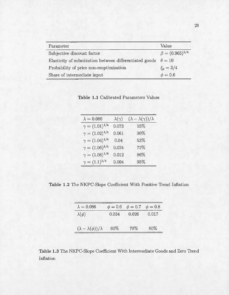
ficient of the KPC. Tables 1.2 - 1.4 provide a quantitative assessment of this

coefficient in the four models described in the previous section. For Ç,p and fJ set

at their baseline values, the slope coefficient of the sticky-priee model without

intermediate inputs and a log-linearization around zero steady-state inflation, À,

is 0.086. Nelson (1998) provides evidence showing that to match the high pos­

itive serial correlation of inflation found in the U.S. data, the standard Calvo

7. See Cogley and Sbordone (2008, footnote 19).

25

sticky-price model with zero trend inflation must assume a very high probability

of priee non-reoptimization, in the neighborhood of 0.9. With Çp = 0.9, the slope

coefficient on marginal cast is then 0.012, or 7 times smaller than implied by our

baseline calibration. The sensitivity of inflation to real marginal cost in the basic

sticky-price madel is too high to match inflation persistence.

Ascari (2004) assesses the sensitivity of the NKPC-slope coefficient to trend

inflation in the sticky-price madel. Table 1.2 reports values of À('Y) corresponding

to alternative levels of trend inflation. For a trend inflation of 2% annually, the

slope coefficient decreases by 30% with respect to a log-linearization around zero

steady-state inflation. If annualized trend inflation is 4%, the slope coefficient

is roughly eut in half decreasing by 53% with respect to the standard model.

However, to generate a slope coefficient of about 0.012 , trend inflation would

have to be 8%. Such a high value of trend inflation is implausible for the U.S.

economy. Indeed, the average rate of U.S. inflation has been 3.57% from 1960:! to

2011:III. · Once dividing the sample period into two subperiods, the average rate

of inflation is 4.92% (roughly 5%) between 1960:! and 1983:IV and 2.4% from

1984:! to 201l:III. Clearly, 8% trend inflation is too high for the KPC with non­

zero steady-state inflation to generate a slope coefficient that would be consistent

with the inertial behavior of inflation. But as emphasized by Ascari (2004), the

findings presented in Table 1 suggest that a log-linear approximation expressing

the dynamics of inflation as a function of the future expected path of marginal

costs in a zero steady-state inflation substantially deteriorates as trend inflation

increases.

Next, we examine the response of inflation to real marginal costs in a sticky­

price madel with intermediate inputs and zero steady-state inflation. Table 1.3

reports the slope coefficient, À ( </;), for 'Y = 1 and a share of inter mediate inputs

cp ranging from 0.6 to 0. 8. With cf> = 0.6, the slope coefficient on marginal cast

is 0.034, which repre ents a huge drop of 60% with respect to the basic sticky­

price mo del ( <P = 0 and Î = 1) . Interestingly, this has more or less the same

effect as assuming an annualized inflation trend of 4. 75% in a madel without

intermediate goods. rote, however, that for a share of intermediate inputs set at

26

0.6, account ing for a roundabout structure with zero trend inflation will not lower

the slope coefficient by enough to be consistent with inflation persistence. This

would require a share of intermediate inputs of 0.8 or higher . St ill , our findings

suggest that adding input-output linkages between firms to a sticky-price madel

with zero-t rend inflation has a stronger impact on inflation dynamics under a

plausible share of intermediate inputs than embedding modest steady-state rates

of inflation in a madel without intermediate inputs.

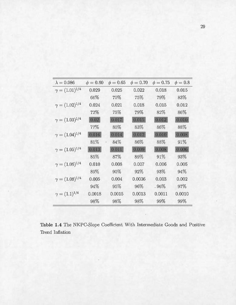
Our last madel combines sticky priees with intermediate inputs and positive

trend inflation. Table 1.4 reports the slope coefficients À(r , 1;) for alternative

values of 1 and cjy. Their joint effect on the NKPC is striking. For example, with

an annualized rate of trend inflation of only 1% and a share of intermediate inputs

of 0.6, the NKPC-slope coefficient is quite small at 0.029, which represents a buge

decline of about 66% with respect to the basic madel with zero t rend inflation

and no intermediate inputs. More importantly, for a trend inflation rate between

3 and 5% and a share of intermediate inputs between 0.6 to 0.8 (the shaded area

in Table 1.4), the slope coefficient on marginal cost varies between 0.006 and

0.02 , which is broadly consistent with short-run inflation dynamics. Furthermore,

even for a t rend inflation rate as low as 1 or 2%, the madel delivers small slope

coefficients insofar as the share of intermediate inputs is high (between O. 7 and

0.8) . Figure 1.1 summarizes the effect of alternative values of 1 and cjy on the

NKPC-slope coefficient, À(/, 1;).

The last question we a..sk is whether t he percentage reductions in the NKPC­

slope coefficient remain large when the frequency of priee adjustments is set at a

higher value. Vve lower Çp from 3/4 to 2/3, which is equivalent to decreasing the

median wait ing time between priee adjustments from 7.2 to 5.1 months. Çp being

lower, the slope coefficient increases. Specifically, in the basic madel, the slope

coefficient À doubles when Çp decreases from 3/4 to 2/ 3 (0.086 vs 0.17). Wit h

such a high frequency of priee adjustments, the standard Calvo-pricing madel

fails dramatically to capture inflation dynamics. The percentage declines in the

slope coefficients corresponding to admissible values of 1 and cjy remain very large,

even at low t rend inflation rates . For a 3% annualized trend inflation rat e, the

------ -·------------------

27

slope coefficient decreases by 73, 79 and 86% if the share of intermediate inputs

is 0.6, 0.7 and 0.8, respectively. Therefore, the impact of positive trend inflation

and roundabout production on the KPC is still very large when the frequency

of priee changes is very high.

1.6 Conclusion

For years , ew Keynesian Phillips Curve models have a..'3sumed zero steady­

state inflation ( e.g. , Christiano, Eichenbaum and Evans, 2005; Smets and Wouters,

2007) , presumably as a matter of convenience. However, a growing body of re­

search tends to demonstrate that this assumption can be misleading, giving a

distorted picture of the sources of inflation dynamics and of the way monetary

policy should be conducted (e.g. , Ascari, 2004; Ascari and Ropele, 2007; Coibion

and Gorodnichenko, 2011).

\Vhile recognizing the significance of accounting for positive trend inflation

in new keynesian models, the present paper has emphasized another important

mechanism contributing to inflation persistence: the multiplier for priee stickiness.

This multiplier arises from the interaction between sticky priees and a realistic

roundabout production structure characterizing modern industrialised economies.

Taken together , positive trend inflation and roundabout production act as pow­

erful mechanims lowering the response of inflation to real marginal costs, and

strongly affecting the Iew Keynesian Phillips Curve. Unifying these promising

mechanisms into DSG E mo dels with nominal rigidities and other types of frictions

should come high on the agenda of future research.

28

Parameter Value

Subjective discount factor (3 = (0.965)114

Elasticity of substitution between differentiated goods e = 10

Probability of priee non-reoptimization Çp = 3/4

Share of intermediate input cp= 0.6

Table 1.1 Calibrated Parameters Values

À= 0.086 À(! ) (À- À(r)) / À

1 = (1.01)1/4 0.073 15%

1 = (1.02)1/4 0.061 30%

1 = (1.04)1/4 0.04 53%

1 = (1.06)1/4 0.024 72%

1 = (1.08)1/4 0.012 86%

1 = (1.1)1/4 0.004 95%

Table 1.2 The NKPC-Slope Coefficient \iVith Positive Trend Inflation

À= 0.086 <P =0.6 <P= 0.7 cp =0.8

0.034 0.026 0.017

(> .. - À( cp)) / À 60% 70% 80%

Table 1.3 The NKPC-Slope Coefficient \rVith Intermediate Goods and Zero T'rend

Inflation

29

À = 0.086 cp = 0.60 cp= 0.65 cp= 0.70 cp =0.75 cp= 0.8

'Y = (1.01)1/4 0.029 0.025 0.022 0.018 0.015

66% 70% 75% 79% 83%

'Y = (1.02)1/4 0.024 0.021 0.018 0.015 0.012

72% 82%

'Y = (1.03)1/4

77% 86%

'Y = (1.04)1/4

81% 88% 91%

'Y= (1.05)1/4

85% 87% 89% 91% 93%

'Y= (1.06)1/4 0.010 0.008 0.007 0.006 0.005

89% 90% 92% 93% 94%

'Y = (1.08)114 0.005 0.004 0.0036 0.003 0.002

94% 95% 96% . 96% 97%

'Y= (1.1)1 /4 0.0018 0.0015 0.0013 0.0011 0.0010

98% 98% 98% 99% 99%

Table 1.4 The NKPC-Slope Coefficient \.Vith Intermediate Goods and Positive

'D.-end Inflation

0 .03

c 0 .025 (l)

(_)

0 .02 ~ (l)

0 (.)

0 .015 (l)

0... 0

({) 0 .01 u 0... ~ :z: 0 .005

0 0 .9

- ·.·

.... . , . . . . .

;. - · ... . -· .

.. · :

..; . ..

·· ··· · · ··· ·· · ·· · ·· · ·~· · ·· · · .. . ·········· · · · -~ . -:~"-'-~~:~~::::.~ ..

.... : : :· .· ... ·· .. : ·:.

30

. .. .

. . . ··· ·. ··_._ ·.·. ·.·.·.· ..... .... .... . ··~.: : -·.· .. · .. ·._··.·. ··. · ... ..... _ .. _.· _.· .·:: : - ·. ·.·.·. ·.·.·.·.·~~0. 1 0 .7 . .... ...... ·.. . . . . 0.06 .

S hare of lnte rm ediat e Input 0 .5 0 A nnual Trend Inflation Rat e

Figure 1.1 The NKPC-Slope Coefficient with Different Values of t rend inflat ion

1 and the share of intermediate goods cp

CHAPTER II

INFLATION PERSISTENCE IN DSGE MODELS: AN EMPIRICAL ANALYSIS

Abstract

This paper simulates a DSGE model >vith roundabout structure of production and

positive trend inflation to a.ssess inflation persistence observed in the U.S . data. Our

simulation results provide empirical evidence in favor of intermediate goods. In effect,

we find that positive trend inflation appea.rs to have a negligible impact on inflation

persistence when allowing for roundabout production. Consequently, the multiplier for

priee stickiness, stemming from t he interaction between sticky priees and intermediate

goods turns out to be the key driving force behind U.S. inflation persistence.

JEL classification: E31, E32.

K eywords: Inflation persistence; roundabout production; positive trend inflat ion.

32

2.1 Introduction

Inflation persistence is considered as the long-run effect of a shock to in­

flat ion - given a shock that raises inflation today by 1%, by how mu ch do we

expect it to be higher at sorne future date and how long (if ever) will it t ake to

return t o its previous level (Pi vetta and Reis, 2007) . This property of inflation

is extremely important to be fully understood especially by central banks, which

are responsible for stabilizing inflation at low levels (Sbordone, 2007).

The main goal of this paper is to improve our understanding of inflation

persistence in a DSGE framework. From this point of view, Ascari (2004) studios

short terms dynamics of inflation through a NKPC's slope coefficient analysis, in

a standard Calvo staggered priee madel allowing for positive steady-state infla­

tion. He shows that positive trend inflation may significantly decrease the slope

coefficient on real marginal costs.

The central critic of dealing with inflation persistence based on the KPC­

slope coefficient is that, inflation dynamics are solely viewed through the variations

of real marginal costs. By doing so, t he impact of other components of the KPC

on inflation dynamics is ignored. Therefore, the contribution of the present paper

is to overcome t he shortcomings of t his type of analytical approach, by proposing

an alternative perspective of the study of inflation persistence. Here, the inflation

persistence analysis relies on the simulation of a model economy, in arder to

account for the contribut ion of a.ll the variables in the economy to short term

dynamics of inflation.

To do so, we build on the work of Phaneuf and Tchakondo (2012). The

authors extend the Ascari (2004) 's DSGE model, to study U.S. inflation persis­

tence in a framework where for the first time, they take in account roundabout

production structure and positive trend inflation. They find, in line with A cari

(2004) that, trend inflation plays a non negligible role in explaining short term

inflation dynamics. They also show that , positive trend inflation and intermediate

goods, taken together , act as powerful mechanisms lowering the response of infla-

33

tion to real marginal costs, and strongly affecting the NKPC . Moreover , Phaneuf

and T chakondo (2012) highlights the multiplier for priee stickiness, arising from

the interaction between sticky priees and intermediate goods as a key source of

inflation persistence.

However , contrary to Ascari (2004), we also embed here various frictions

such as habit formation, costs of adjustment in capital accumulation and variable

capital ut ilization. The rationale behind this is that , these frict ions have become

quite st andard in the DSGE li terature, and seem to be unavoidable to capture the

empirical persistence in the macroeconomie data (CEE, 2005; Smets and Vvouters,

2003) . In fact , the habit formation in consumption is used to reveal the necessary

empirical persistence in the consumption process (see, e.g. , Bouakez, Cardia and

Ruge-Murcia, 2005; Smets and Wouters, 2003; Fuhrer, 2000; and McCallum and

Nelson, 1999) . The capital adjustments cost s do play a critical role in account ing

for the dynamics of investment , since they induce inert ia in investment , causing

it to adjust slowly to shocks (see, e.g., Groth and Khan, 2006; CEE, 2005; and

Smets and \Vouters, 2003) . Finally, the variable capital ut ilization rate aims at

smoothing the adjustment of the rentai rate of capital in reaction to changes in

output (see, e.g., Khan and Tsoukala..s, 2012; CEE, 2005; Smets and Wouters,

2003; King and Rebelo, 2000).

Then, from the overall madel, we simulate five specifie typ es of models. The

first one is the madel with sticky priees, zero-trend inflation without intermediate

goods and real frictions. Vve refer to this madel as t he ba..sic Calvo madel or SP

madel with SP standing for sticky priees. Adding t he real frict ions ment ioned

earlier to the basic Calvo madel gives rise to the SP-RF madel where RF st ands

for real frictions. Furthermore, the t hird madel is t he SP-RF madel with posit ive

trend inflation without intermediate goods, called the SP-RF-PT madel wit h PT

indicating positive t rend. The fourth madel is the SP-RF madel with .intermedi­

ate goods but without positive trend inflation, say, the SP-RF-RP madel where

RP means roundabout production. Finally, the SP-RF madel with intermediate

goods and positive t rend inflation, t he SP-RF-RP-PT madel, is considered as our

benchmark madel.

34

In addition, we generate from each specifie simulated model the autocar­

relations coefficients of inflation. These theoretical autocorrelations coefficients

of inflation are in turn compared with those suggested by tJ.S. data. Vve show

that , in order for the SP model to replicate the data, the probability of priee

non-reoptimization must be set at a high level around 0.96, implying an average

waiting time between priee adjustments of 6.25 years. For the SP-RF model ,

the probability must be close to 0.9 , suggesting an average wa.iting t ime between

priee adjustments of 2.5 years or more, which is clearly counterfactual. As a conse­

quence, the basic Calvo model even improved, is hardly reconcilable with inRation

persistence unless assuming an implausibly low frequency of priee adjustments.

\ iVith regard to the The SP-RF-PT model, we find that trend inflation

must almost reach 11% to account for inflation persistence observed in U.S. data.

Such a high value of trend inflation is unlikely for the U .S. economy. The SP­

RF-RP model suggests a share of intermediate goods above 0.7 to be consistent

with inflation persistence. For the SP-RF-RP-PT model, our findings suggest

that, for realistic levels of trend inflation, intermediate goods supersede positive

trend inflation in accounting for inflation persistence. For instance, with a share

of intermediate goods set at 0.7, the autocorrelation coefficients of inflation are

decreasing with positive trend inRations ranging from 1% to 5%, and are alllesser

than those obtained with zero-trend inflation. Therefore, positive trend inflation

appears to have a negligible impact on inflation persistence when allowing for

intermediate goods. In other words, the multiplier for priee stickiness, stemming

from the interaction between sticky priees and intermediate goods turns out to be

the key driving force behind inflation persistence.

Finally, when t he frequency of priee adjustments is high with a probability

of priee non-reoptimization set at 2/3, our results also highlight the negligible

contribution of trend inflation to inflation dynamics when taldng in account inter­

mediate goods. So, the scope of positive t rend inflation stressed in the literature

as in Ascari (2004) , appears to be overestimated and exaggerated in the presence

of rounda.bout structure of production.

35

The rest of the paper is organized as follows. Section 2 describes t he model

economy. Section 3 discusses calibration issues. Section 4 presents the empirical

evidence regarding inflation persistence in the U.S. economy and our main results.

Section 5 concludes.

2.2 The Model Econ01ny

The madel economy consists of households, a representative final good pro­

ducer, a continuum of intermediate goods producers indexed by j E [0, 1] and a

government conducting monetary policy.

2.2.1 Households

Households consume goods and services, supply a labor to labor market ,

rent capital services to firms , and make investment and capital utilization deci­

sions. There are costs related t o adjusting the flow of investment and capital

ut ilization decisions.

The ut ility function is the same as Chari, Kehoe and :tvicGrattan (2010) but

features the habit formation as in Christiane, Eichenbaum and Evans (2005). So,

the preferences of the representative household are given by

where j3 E (0, 1) denotes t he subjective discount factor, Ct is consumpt ion of

final good, Mt is nominal stock of money, Pt is the priee of final good , jVft/ Pt is real

money balances , Lt is labor. Et indicates the conditional expectation operator ,

b is the utility weight of consumption, h is the habit formation parameter in

consumpt ion preferences , Tl is interest elasticity, e is the weight on leisure, and x denotes a risk aversion coefficient.

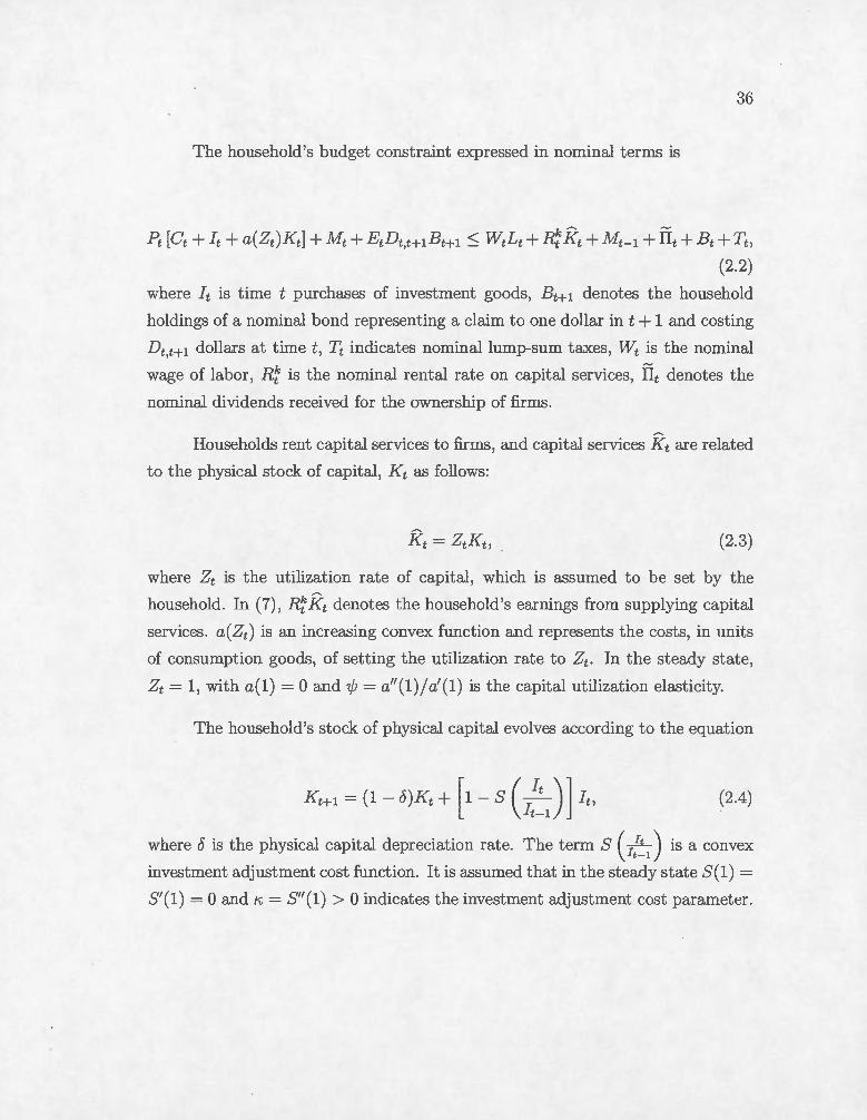
36

The household 's budget constraint expressed in nominal ter ms is

k~ -Pt [Ct+ It + a(Zt)Kt] +Mt+ EtDt,t+lBt+l ~ WtLt + Rt Kt+ Mt-1 + llt + Bt +Tt ,

(2.2) where It is time t purchases of investment goods, Bt+l denotes the household

holdings of a nominal bond representing a daim to one dollar in t + 1 and casting

Dt,t+l dollars at time t, Tt indicates nominal lump-sum taxes, ltVt is the nominal

wage of labor , R': is the nominal rentai rate on capital services, Dt denotes the

nominal dividends received for the ownership of firms.

~

Households rent capital services to firms , and capital services Kt are related

to the physical stock of capital, Kt as follows:

(2.3)

where Zt is the utilization rate of capital, which is assumed to be set by the

household. In (7) , J?!! Kt denotes the household 's earnings from supplying capital

services. a(Zt) is an increasing convex function and represents the costs, in units

of consumption goods, of setting the utilization rate to Zt. In the steady state,

Zt = 1, with a(l) = 0 and 'ljJ = a"(l)/a'(l) is the capital utilization elasticity.

The household 's stock of physical capital evolves according to the equation

(2.4)

where 6 is the physical capital depreciation rate. The tenn S ( 1t1~ 1 ) 1s a convex

investment adjustment cost function. It is assumed that in the steady state S(1) =

S'(1) = 0 and"'= S"(1) > 0 indicates the investment adjustment cost parameter.

37

2.2.2 Firms

Let Xt (j) be the quantity of differentiated goods produced by firrns j for

j E [0 , 1] , and let Pt(j) be the nominal priees . The aggregate production, Xt , is a

composite of differentiated goods, Xt(j) , and produced in a perfectly competitive

sector such that:

1 Xt = [f Xt(j)(B-1) /B dj]BI(B-1) ' (2.5)

0

where B E (1 , oo) is the elasticity of substitution between the goods . The corre­

sponding priee index, Pt, is the priee of the composite good related to t he priees,

Pt(j) , and expressed as:

(2.6)

The demand function for good of type j resulting from optimizing behavior

in the aggregation sector is given by

(2.7)

The production of good j requires the use of capital, labor , and intermediate

inputs:

(2.8)

where r t(j) is the input of intermediate goods, Kt(j) is the input of capital ser­

vices, Lt(j) denotes total hours worked, and F is a fixed cost which is identical

across firms. The parameter cp E (0 1) measures the elasticity of output with

respect to intermediate input , and the parameters ·a E (0 , 1) and (1 -a) are the

elasticities of value-added with respect to the capital and labor input , respectively.

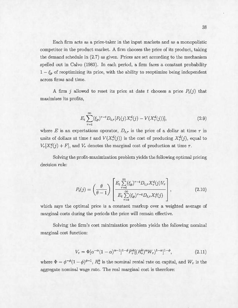
38

Each firm acts as a price-taker in the input market s and as a monopolistie

competitor in the product market. A finn ehooses the priee of its product , taking

the demand schedule in (2. 7) as given. Priees are set according to the mechanism

spelled out in Calvo (1983). In each period , a firm faces a const ant probability

1 - Çp of reopt imizing its priee, with the ability to reopt imize being independent

across firms and time.

A firm j allowed to reset its priee at dat e t chooses a priee Pt()) that

maximizes its profits,

00

Et l:: (Çpf'-tDt,T[Pt Cf)X~(j)- V(X~(j))J, (2.9) T=t

where E is an expectations operator , Dt,T is the priee of a dollar at time T in

units of dollars at t ime t and V(X~(j ) ) is the cost of producing X~(j) , equal to

V7 [X~(j) + F ], and V7 denotes the marginal cost of production at t ime T .

Solving the profit-maximization problem yields t he following optimal pricing

decision rule:

(2.10)

which says the opt imal priee is a const ant markup over a weighted average of

marginal costs during the periods the priee will remain effective.

Solving the firm 's eost minimization problem yields the following nominal

marginal cost function:

(2.11)

where 4? = cp-<P (1- cp) rf>-1, R~ is the nominal rental rate on capital, and W7 is t he

aggregate nominal wage rat e. The real marginal cost is therefore:

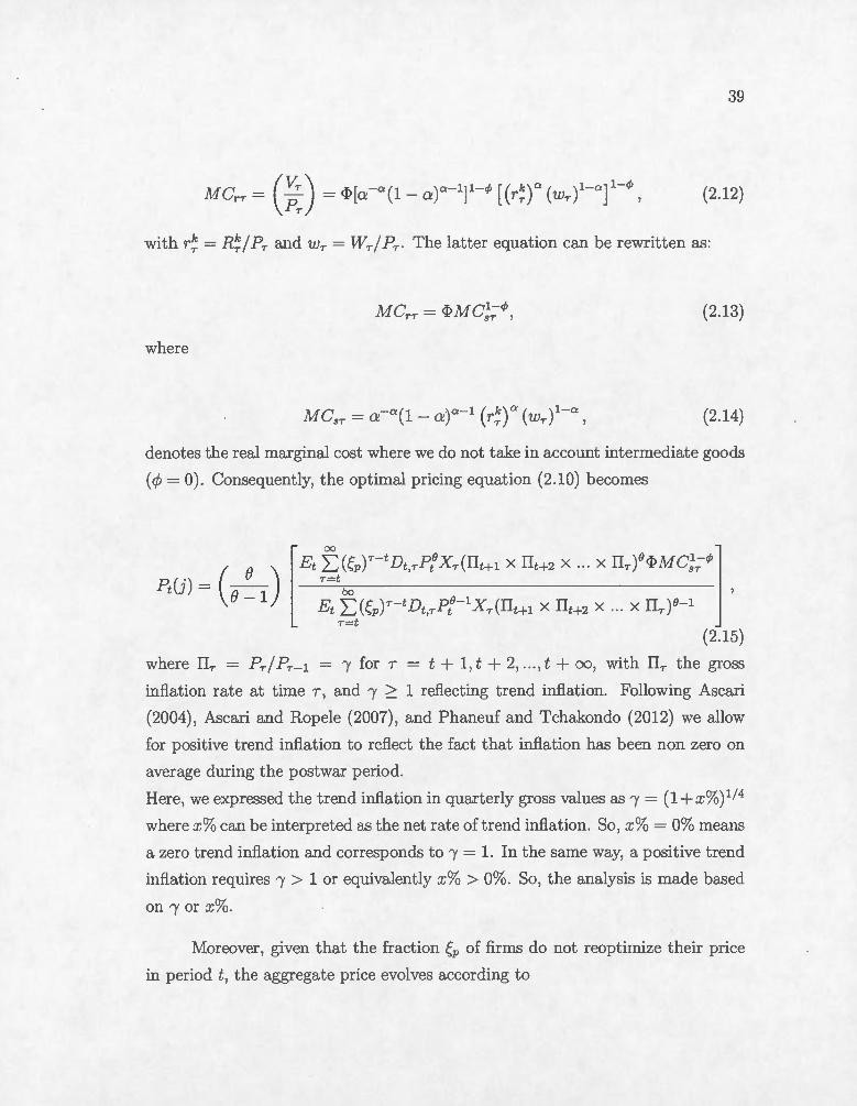
39

(2.12)

with r~ = R~/ Pr and Wr = liVr/ Pr. The latter equation can be rewritten as:

(2.13)

where

Mc -0' (1 )0'-1 ( k) ll' ( )1-0' - sr = Cl:" - Cl:" r r Wr , (2.14)

denotes the real marginal cost where we do not take in account intermediate goods

(cp = 0). Consequently, the opt imal pricing equation (2.10) becomes

( e ) [ Et~ (Çvf-t Dt,rPl X r( IIt+l x IIt+2 x ... x IIr )

0<PMc_;;<t> 1 Pt(j) = -- r-t bo '

O- 1 Et .Z..: (Çv)r-t Dt,rPt0 -1 Xr(IIt+1 x IIt+2 x ... x IIr )0- 1

r=t (2.15)

where IIr = Pr/ Pr_1 = 1 for T = t + 1, t + 2, ... , t + oo, with IIr the gross

inflation rate at time T , and 1 2': 1 reflecting trend inflation. Following Ascari

(2004) , Ascari and Ropele (2007) , and Phaneuf and Tchakondo (2012) we allow

for positive trend inflation to reflect the fact that inflation has been non zero on

average during the postwar period.

Here, we expressed the trend inflation in quarterly gross values as 1 = (1 +x%) 114

where x% can be interpreted as the net rate of trend inflation. So , x% = 0% means

a zero trend inflation and corresponds to 1 = 1. In the same way, a positive trend

inflation requires 1 > 1 or equivalent ly x% > 0%. So, the a.nalysis is made based

on 1 or x%.

Moreover, given tha.t the fraction Çp of firms do not reoptimize their priee

in period t , the aggrega.te priee evolves according to

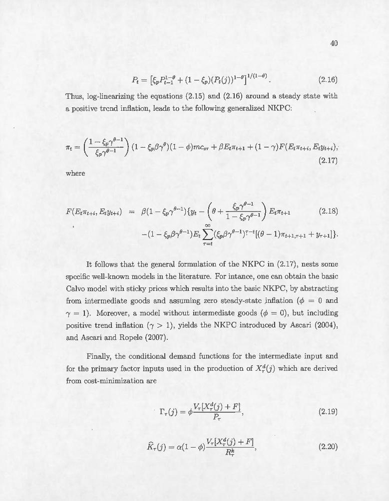
1 •

40

(2.16)

Thus, log-linearizing the equations (2.15) and (2.16) around a steady state with

a positive trend inflation, leads to the following generalized NKPC:

where

(2.18)

00

-(1- Çp/3·/-1)Et 2::)Çp/3·l'-1t-t[(e- 1)7rt+l,-r+l + YT+l]}. T=t

It follows that the general formulation of the NKPC in (2.17), nests sorne

specifie well-known models in the literature. For intance, one can obtain the basic

Calvo model with sticky priees which results into the basic NKPC, by abstracting

from intermediate goods and assuming zero steady-state inflation (cp = 0 and

1 = 1). Moreover, a model without intermediate goods (cp = 0), but including

positive trend inflation (! > 1 ), yields the KPC introduced by Ascari (2004),

and Ascari and Ropele (2007).

Finally, the conditional demand functions for the intermediate input and

for the primary factor inputs used in the production of x:(j) which are derived

from cost-minimization are

r ( .) = ,~, vT[x:(j) + F] T) 'f' p )

T

(2 .19)

R ( .) = (1 _ "') vT[x:(j) + F] T J a 'f' Rk '

T

(2.20)

41

and

(2.21)

2.2.3 Monetary Policy

The government injects money into the economy through nominal transfers,

so 1t = .Ni l - Mf_1 where M 8 is the aggregate nominal money supply. Further­

more, following Ascari (2004) and Ascari and Ropele (2007), we assume that

steady-state money supply evolves according to the fixed rule: .Arif = r 1Vlf_1 ,

where 1 is the gross steady-state growth rate of nominal money supply and the

source of positive trend inflation.

2.2.4 Equilibrilnn and 1v1arket-Clearing Conditions

An equilibrium consists of allocations ft(j) , Kt(j), Lt(j) and priee Pt(j)

for firm j , for all jE [0, 1], together with priees D t ,t+l, Pt , Rf, and Vfl t , satisfying

t he following conditio"ns: (i) taking the nominal wage rate and all priees but its

own as given, each firm 's allocations and priee solve its maximization problem;

(ii) markets for bonds, capital, labor and the composite good clear; (iii) monetary

policy is as specified.

Along with (2.19) , the market-clearing condition for the composite good

1

yt + f f t(j)dj = Xt, 0

implies that equilibrium real GDP is related to gross output by

(2.22)

where Gt = JJ [Pt(j)/ Pt]- 8 dj captures the priee-dispersion effect of staggered priee

con tracts.

42

Meanwhile, t he market-clearing condit ions JJ Kf(j)dj = Kt for capital ser­

vices, and JJ Lf(j)dj = Lf = L: for labor , along with (2.20) and (2.21) , imply that

the equilibrium aggregate capital services and labor are related to gross output

by

(2.23)

Vt Lt = (1 - a)(1- </> )lVt [GtXt + FJ. (2.24)

Equations (2.22) , (2 .23) , and (2.24) , together with the price-setting equation

(2.10) , characterize an equilibrium.

The overall resource constraint of the economy is given by

(2.25)

2.3 Calibration

We need to assign values to the following parameters: the subjective dis­

count factor /3, the preference parameters b, h, 'TJ , e, x, the technology parameters

<P and a , the elasticity of substit ution between differentiated goods e' the capital

depreciation rate <5 the capital adjustment cost parameter K , the capital utiliza­

t ion elasticity 'lj;, and t he probability of priee non-reopt imization Çp. The values

assigned to these parameters are summarized in Table 2.2.

The subjective discount factor is f3 = (0.965)114. The preference parameters

are taken from Chari, Kehoe and McGrattan (2000) , so 'Tl = 0. 39, b = 0.94, e = 1.5

and x= 1. 1 The habit formation parameter h ranges from 0.59 as in Smets and

Wouters (2003) to very high values of 0.98 as reported by Bouakez, Cardia and

1. The same values are used by Asca.ri.

43

Ruge-Murcia (2005) . Ravn, Schmitt-Grohe, and Uribe (2006) and Ravn, Schmitt­

Grohé, Uribe and Uusakala (2008) give a value of 0.86 to 0.85 respectively. We set

this value to 0.8 as in Fuhrer (2000) and Boldrin, Christiano and Fisher (2001) .

The elasticity of substit ution between differentiated goods e determines

the steady-state markup of priees over marginal cost , with t he markup given by

P,p = ej(e -1). As in Chari, Kehoe and McGrattan (2000) and Ascari (2004) e is

set to 10, so the value-added markup is 1.11. The steady-state ratio of the fixed

cost to gross output F / X is set accordingly, so that the steady-state profits for

firms are zero (and there will be no incent ive to enter or exit the industry in the

long run). The elasticity of value-added with respect t o capital input a is 0.33,

and the capital depreciation rate o = 1 - (0.92) 114.

The capital adjustment cost parameter K captures the costs associat ed with

changing the level of capital. We know from Groth (2006) that this parameter

could range from 0 to infinity. For inst ance, Woodford (2003) proposes a value of

3. Eichenbaum and Fisher (2004) firid that for K equal to or above 3, t he implied

priee duration is less than one year , t hus consistent with evidence from micro­

studies. The same evidence is found by Gagnon and Khan (2005) for the case

when K goes to infinity. Conversely, when K is below 3, estimates of the NKPC

are less able to match micro data on the duration of priees. Furthermore, based

on the results from q models literature, Groth (2006) finds a value of K between 40

and 80 ac; in Eichenbaum and Fisher (2004). Meanwhile, based on the parameter

estimates reported by Shapiro (1986), Groth (2006) obtains a value of K equal to

17, and the estimates by Groth (2005) imply a value of K = 20. Therefore, we

choose K = 10. The capital utilization elac;ticity 'ljJ is fL-xed at 1 (Basu and Kimball ,

1997; Dotsey and King, 2006).

The parameter cp measures the share of payments to intermediat e input in

total production cost or cost share. With markup pricing, it equals the product

of the steady-state markup and t he share of intermediate input in gross output

or revenue share. \lVe rely on two different sources of dat a to calibrat e cp for

the postwar U.S. economy. The first source is a study by Jorgenson, Gollop

44

and Fraumeni (1987) suggesting that the revenue share of intermediate input in

total manufacturing output is about 50 percent. \iVith a steady-state markup of

1.11 , this implies cp = 0.56. The second source relies on the 1997 Benchmark

Input-Output Tables of the Bureau of Economie Analysis (BEA, 1997). In the

Input-Output Table, the ratio of "total intermediate" to "total industry output"

in the manufacturing sector or revenue share is 0.68, implying cp = O. 75. Renee,

according to our two alternative sources of data, admissible values of cp range from

0.56 to 0.75. Bergin and Feenstra (2000) assume even higher values of cp , from

0.8 to 0.9, which appears excessively high based on our calculations. HuaJlg, Liu

and PhaJleuf (2004) and Nakamura and Steinsson (2010) choose cp = 0.7 as a

benchmark for the postwar U.S. economy. So, we set cp at 0.7. However, for the

sensit ivity analysis we also consider other values of cp.

The parameter Çp, which measures the probability of priee non-reoptimization,

is fixed as follows. In a survey of postwar evidence on U.S . priee behavior, Taylor

(1999) documents that priees have changed about once a year on average. Using

summary statistics from the Consumer Priee Index micro data compiled by the

U .S. Bureau of La bor Statistics for 350 categories of consumer goods and ser­

vices, Bils and Klenow (2004) document that the median waiting time between

priee adjustments has been 4.3 months when priee adjustments occuring during

temporary sales are taken into account, while it has been 5.5 months when they

are not. Their evidence, however, covers only a very short period of time, the

years 1995-1997. Using a fewer categories of consumer goods and services, they

report evidence suggesting that for the longer period 1959-2000 the frequency of

priee adjustments is significantly lower than for the years 1995-1997. Nakamura

and Steinsson (2008) provide estimates of the frequency of priee changes ranging

from 8 to 11 months when product substitutions and temporary sales are both

excluded, and from 7 and 9 months when only temporar:y sales are excluded.

Moreover , Bils and Klenow (2004) empha..size the median as their measure ofwait­

ing time between priee adjustments. Approximating the waiting time to the ne:>...'t

priee change by Ç~ , the median waiting time between priee changes is given by

45

-ln(2)/ ln(Çp) · 2 Setting Çp = 3/4 implies that the median waiting time between

priee changes is 7.2 months, which is in the range of admissible values from micro

level evidence. At macro level, Justiniano, Primeceri and Tambolotti (2011) es­

timate the probability of priee non-reoptimization, in a DSGE model using U.S.

_ quarterly data from 1954QIII to 2009QI. They find that Çp ranges from O. 757 to

0.817.

In light of these studies , we set the ba..c;eline value of Çp at 3/4 ( see also Ascari ,

2004; Ascari and Ropele 2007). We la ter assess the sensitivity of our findings to

lowering Çp.

2.4 Results

First , we document in this section, for U .S. data, the main empirical fact

that is the focus of this paper: inflation persistence - considered here as the high

and slowly decaying positive autocorrelations of the quarterly first difference of

the log GDP deflator (Nelson, 1998) . The data used are the nonfarm business

sector GDP deflator data (Pt), which are obtained from the Federal Reserve Bank

of St. Louis' database. These data begin in 1959:1 and end in 2013:2.

Let 7ït indicate inflation (6.logPt) and p1i(J.L) the j.tth autocorrelation of 7ït·

Following Nelson (1998), we generate simple autocorrelations coefficients of infla­

tion. The values are summarized in Table 2.1. Table 2.1 shows that the first-order

autocorrelation coefficient of inflation p1i(J.L) = 0.83. Inflation's higher-order au­

tocorrelations are also large, remaining above 0.5 even at lag six. It follows that

inflation displays considerable persistence.

Second, to a..c;ses the role and the importance of accounting for roundabout

production in U.S . inflation persistence, we simulate several types of models de­

rived from the generalized NKPC in (2.17). For each simulated mo del , we generate

the autocorrelations coefficients of in.fl.ation. These theoretical autocorrelations

coefficients of inflation are then compared with the data presented in Table 2.1.

2. See Cogley and Sbordone (2008, footnote 19).

46

The first simulated model is the basic Calvo model with sticky priees, zero

steady-state inflation (x% = 0%) without intermediate goods ( <P = 0) , habit for­

mation, capital adjustment costs and ut ilization rate of capital. The autocorrela­

tion coefficients of inflation of this model compared to the data are presented in

Figure 2.1. The results suggest that in order for the basic Calvo model to replicate

the data, the probability of priee non-reopt imization must be set at a high level

around 0.96, implying an average waiting t ime between priee adjustments of 6.25

years . This is not consistent with microeconomie evidence on U.S. priee dynamics

documented by Bils and Klenow (2004) and Nakamura and Steinsson (2008), who

suggest respectively a median waiting t ime between 4.3 and 5.5 mont hs, and, 7

and 11 mont hs for priee adjustments.

The results from the simulated SP-RF model in Figure 2.2 show this prob­

ability must be close t o 0.9. So, the average waiting t ime between priee adjust­

ments is 2.5 years or more , which clearly is counterfactuaJ. Consequently, the

basic Calvo model even improved , is hardly reconcilable with inflation persistence

unless assuming an implausibly low frequency of priee adjustments.

Here, we consider the standard Calvo sticky-price model with posit ive trend

inflation without intermediate goods and the various frictions mentioned above,

as in Ascari (2004). This model is referred to as the SP-PT model. Before going

through the dynamics of inflation, it 's important to highlight some feature of

such an economy relative to the output . In part icular, we a..ssess the reaction of

output to a monetary shock when varying t rend inflation. F igure 2.3 shows the

impulse responses of output to a 1% rate of money growth shock, for different

vaJues of trend inflation (x%), the same like those obt ained by Ascari (2004, fig.

5). Following the shock, the output increases on impact by almost 20% for a trend

of 2.5%, 40% for a t rend of 7.5% and 90% for a level of trend of 10%. This huge

impact effect seems to be unreasonable and at the odds with the evidence about

the impact of monetary policy on real economy.

However , this impact effect becomes much more low and reaJistic in the

SP-RF-PT model, when allowing for the real frictions as we can observe in Figure

47

2.4. Output increases by only 1% for a t rend of 2.5%, 1.2% for a t rend of 7.5% and

2% for a trend of 10%. In addition to dramatically lowering the impact effect , our

benchmark model also accounts for t he delayed, hump-shaped response of output.

It turns out that , tracking the dynamics of output and other macroeconomie

variables like inflation in a DSGE model framework without these frictions as

in Ascari (2004), could be misleading. That 's the reason why, from now on, the

analysis of the cont ribution of positive trend inflation, roundabout production and

their interaction t o inflation persistence, is done based on our benchmark model

rather than the standard Calvo sticky-price model.

In that ca.se, the simulation of the SP-RF-PT model gives t he resul ts pre­

sented in Figure 2.5. These results suggest that trend inflation, x% , must at lea.st

reach 11% to account for inflation persistence observed in U.S. dat a . This seems

unrealistic sin ce the average rate of inflation experienced by the U .S. economy dur­

ing the 1960s and 1970s, a time of high inflation is almost 5%. Consequent ly, the

model with positive trend inflation matches inflation persistence unless a'3suming

very high values of trend inflation.

Figure 2.6 shows the findings for the SP-RF-RP model suggesting a share

of intermediate goods above 0.7 to be consistent with inflation persistence. In

particular, for cp = 0.75, the highest value of the range, the model is about to fit

the data.

However, the SP-RF-RP model has a stronger effect on inflation persistence

under a plausible share of intermediate inputs than the SP-RF-PT model. As

presented in Figure 2.7, for a share of intermediate inputs equa.l to 0.6 and 0.7,

the SP-RF-RP model has respectively the same or more impact on t he dynamics

of inflation than the SP-RF-PT model with a posit ive t rend inflation of 9% and

10%.

The last simulated model is t he benchmark model or the SP-RF-RP-PT

model. Figure 2.8 reports the autocorrelations coefficients of inflation for different

values of trend inflation and a share of intermediat e goods set at a low value of 0.6.

Most surprisingly, t he autocorrelations coefficients for the model with zero-t rend

48

inflation are exactly the same than those obtained with realistic trend inflations

of 1% to 5%. But, these coefficients are slightly lower than the case where trend

inflation is set at a higher level of 10%. ext, we do the same analysis with the

share of intermediate goods set at 0.7, the post world war benchmark value, and

the results are presented in Figure 2.9. Here, the autocorrelation coefficients of

inflation are decreasing with positive trend inflations ranging from 1% to 5% and

are alllesser than those obtained with zero-trend inflation.

As a consequence, for realistic levels of trend inflation, intermediate goods

supersede positive trend inflation in accounting for inflation persistence. In other

words, in a sticky priee economy with intermediate goods and positive trend in­

flation , the multiplier for priee stickiness dominates positive trend inflation when

assessing th short term dynamics of inflation. Even though the positive effect

of the interaction between both ingredients on these dynamics is highlighted in

Phaneuf and Tchakondo (2012) through the NKPC-slope coefficient analysis, the

simulation of the mo del economy reveals a negligible contribution of positive trend

inflation to inflation persistence vvhen allm:ving for intermediate goods. Therefore,

the scope of positive trend inflation suggested in the literature as in Ascari (2004) ,

and Phaneuf and Tchakondo (2012) , appears to be overestimated and exaggerated

in the presence of roundabout structure of production.

Finally we extend the simulation analysis to the case when the frequency

of priee adjustments is high with the probability of priee non-reoptimization set

at 2/3. Our result confirms the previous finding that the basic model is far away

from the reality. Even if The SP-RF model improves inflation persistence, it is not

able to replicate the data. As far as the positive trend inflation is concerned, the

results suggest unrealistic levels of trend inflation around 17% to match inflation

persistence. Moreover, for a share of intermediate goods set at 0.7, the impact of

the SP-RF-RP model on inflation persistence is not quite sufficient to fit the data.

Since the probability of priee non-reoptimization is low, the multiplier of priee

stickiness is less stronger than the previous ca..c;e where Çp = 3/4. Nevertheless,

the autocorrelation coefficients here are greater than those obtained when allovring

for po itive trend inflation. As a matter of fact, the autocorrelation coefficients

49

of the SP-RF-RP-PT model are decreasing in different levels of trend inflation up

to 10%, and are alllesser than those generated from the SP-RF-RP model.

These findings , in some way, corroborate our previous conclusions that when

allowing for the intermediate goods, the effect of positive trend inflation on infla­

tion persistence is negligible. This highlights the predominance of the multiplier

for priee stickiness on the positive trend inflation, in accounting for short term

dynamics of inflation.

2.5 Conclusion

We have simulated a DSGE model featuring intermediate goods and positive

trend inflation alongside other real frictions, in order to examine U.S. inflation

persistence observed in the data. V/e show that the scope of positive trend inflation

stressed in the literature as an importance source of inflation persistence, appears

to be overestimated and exa.ggerated in the presence of roundabout structure of

production. As a. consequence, the multiplier for priee stickiness, arising from the

interaction between sticky priees and intermedia.te goods turns out to be the key

source of U.S . inflation persistence.

--- - ----------------

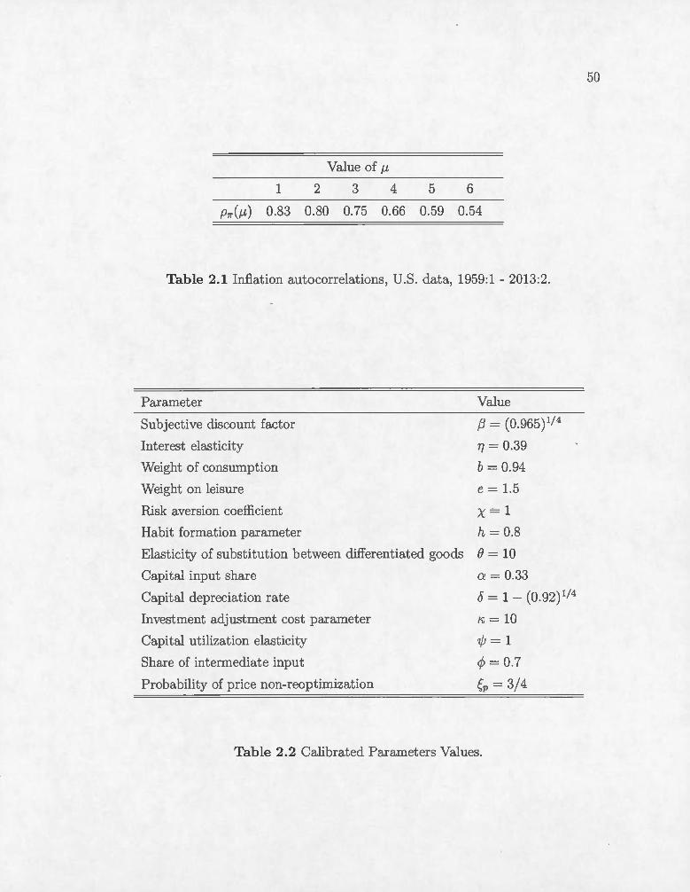
Value of J1

1 2 3 4 5 6

p.,. (J1) 0.83 0.80 0.75 0.66 0.59 0. 54

Table 2.1 Inflation autocorrelations, U.S. dat a, 1959:1 - 2013:2.

Parameter

Subjective discount factor

Interest elasticity

Weight of consumption

vVeight on leisure

Value

{3 = (0.965)114

TJ = 0.39

b = 0.94

e = 1.5

Risk aversion coefficient x = 1

Habit formation parameter h = 0.8

Elasticity of substitution between clifferentiated goods e = 10

Capital input share a = 0.33

Capital depreciation rate 5 = 1 - (0.92) 114

Investment adjustment cost parameter

Capital utilization elasticity

Share of intermediate input

Probability of priee non-reopt imization

ri, = 10

'I/J =1 <P = 0.7

~p = 3/4

Table 2 .2 Calibrated Parameters Values.

~ ------------------------ - --

50

,--------------------------------------------------------------------------------------------

.9

.8

.7

c Cl) .6 (J

Il= -Cl) .5 0

(..)

c 0

.4 -ct)

~ .._ .3 0

(..) 0 -:::l .2 <t

.1

.0 2 3 4

Order

l

-e- data ---o- 3/4 --*'- 0.91 . --- 0.95 -Ir- 0.96 .

51

5 6

Figure 2.1 Autocorrelation Coefficients with Different Values of the Calvo prob­

ability Çp in the SP Model. ·

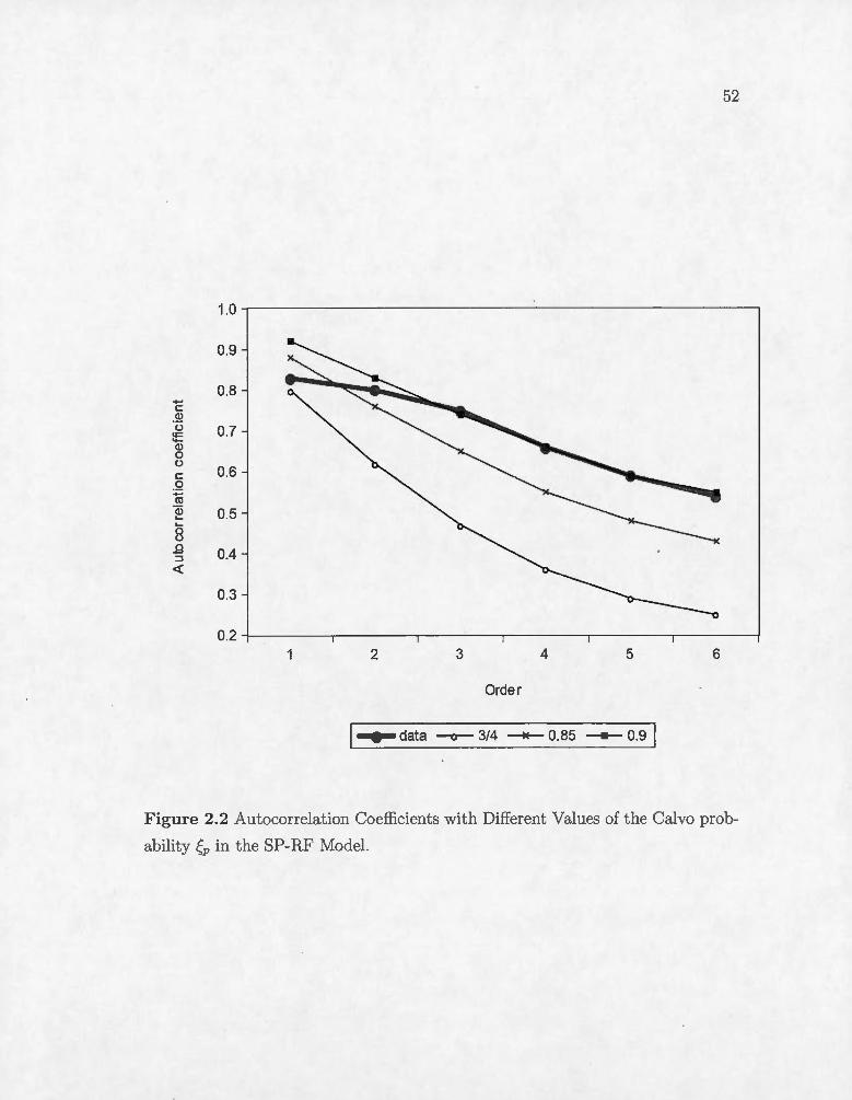
52

1.0

0.9

0.8 ë - ~ (.) 0.7 <;::: ..... Q) 0 (.)

0.6 c .Q ro Q5 0.5 '-

8 .9 0.4 ::J <(

0.3

0.2 2 3 4 5 6

Order

l-e- data --a- 3/4 --w- 0.85 ----- 0.9 1

Figure 2. 2 Autocorrelation Coefficients with Different Values of the Calvo prob­

ability Çp in the SP-RF l\.1odel.

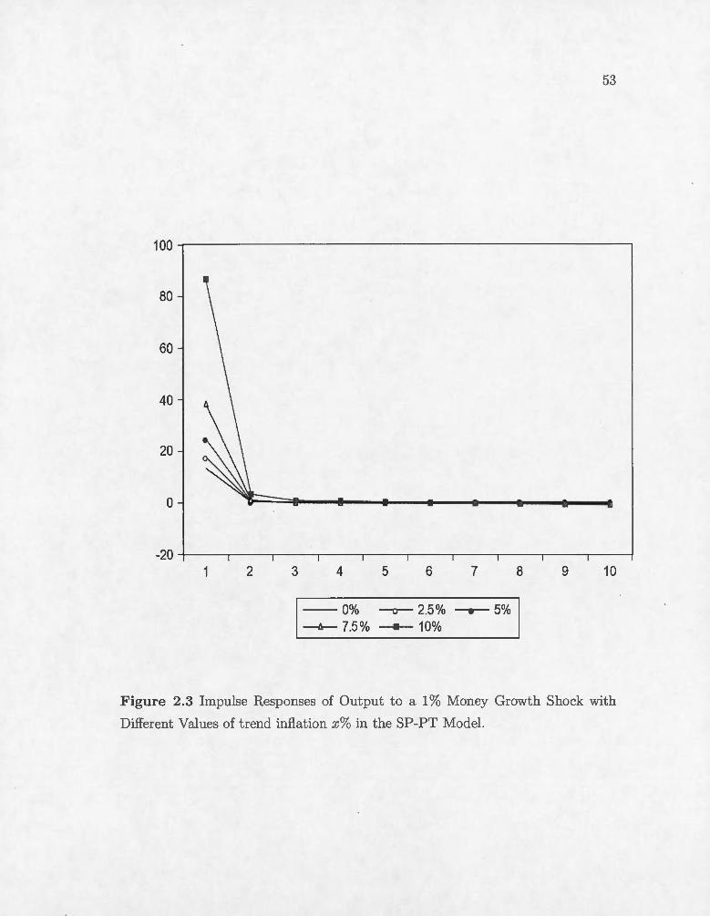
53

2 3 4 5 6 7 8 9 10

-- 0% -o-- 2.5% -.---- 5% --l!r- 7.5% -+--- 10%

Figure 2.3 Impulse Responses of Output to a 1% Money Growt h Shock with

Different Values of t rend inflation x% in the SP-PT Model.

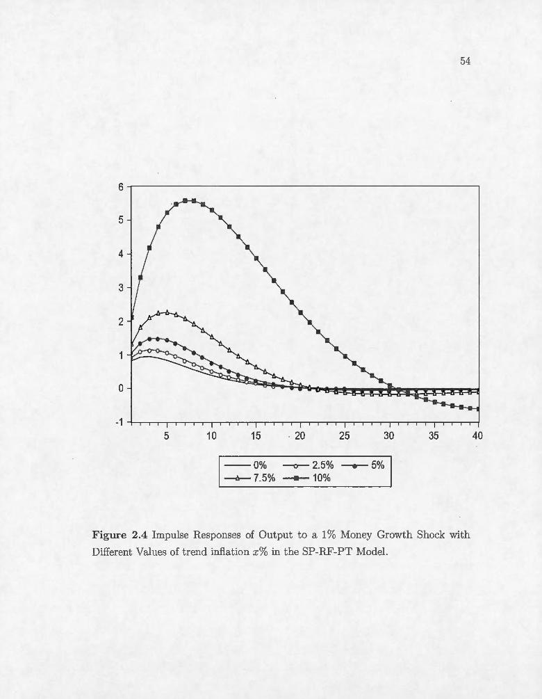
54

5 10 15 . 20 25 30 35

--0% --o- 2.5% --.-- 5% --l:r- 7.5% ---- 10%

Figure 2.4 Impulse Responses of Output to a 1% Ivloney Growth Shock with

Different Values of t rend infl ation x% in the SP-RF-PT Model.

40

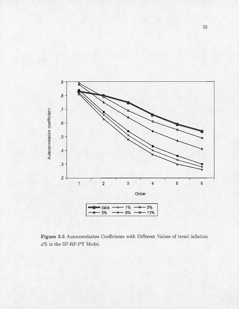
.9

.8

c .7 .~ (.)

""' '+-Q) .6 0 (.)

c .Q - .5 co Q) ..... .....

8 .4 .9 ::J

<t:

.3

.2 2 3 4

Order

~data ~ 1% ---*- 3% ----- 5% _.__ 9% -o-- 11 %

55

5 6

Figure 2. 5 Autocorrelation Coefficients with Different Values of trend inflation

x% in the SP-RF-PT Model.

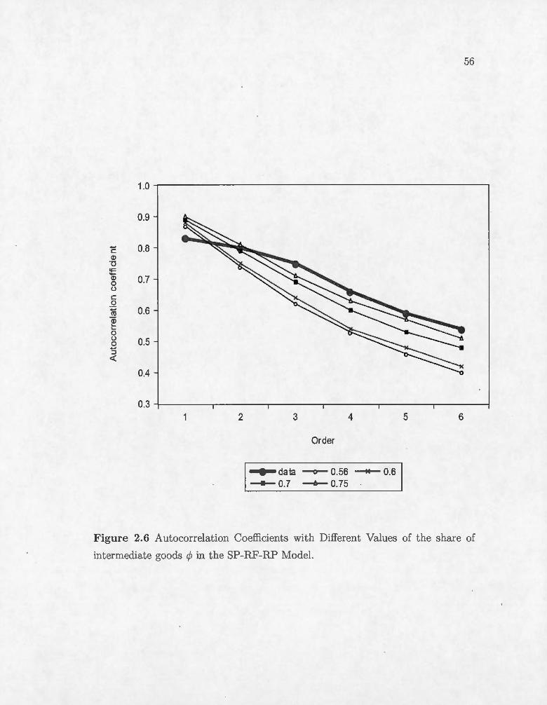
56

1.0

0.9

- 0.8 c (!) ·o '+= .._ (!) 0.7 0 (.)

c _g - 0.6 ct! (!) 1-1-

0 (.) 0.5 0 ..... :::l <{

0.4

0.3 2 3 4 5 6

Or der

Figure 2.6 Autocorrelation Coefficients with Different Values of the share of

intermediate goods cp in the SP-RF-RP ModeL

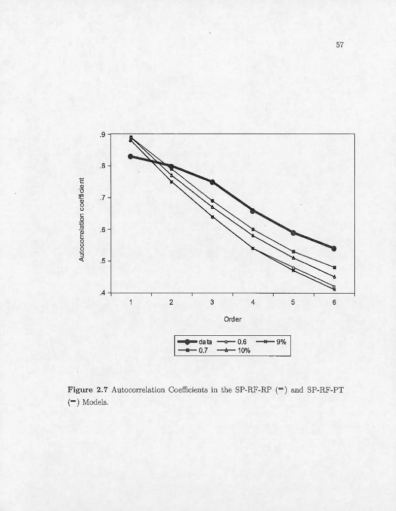
57

.8

...... c (!)

"(3

<+= .7 '+-(!) 0 ü c .Q ...... ro .6 (i) ..... ..... 0 ü 0 -::l <( .5

.4

2 3 4 5 6

Order

~-daia -o-- 0.6 --9%1 --6-10% --- o.?

Figure 2. 7 Autocorrelation Coefficients in the SP-RF-RP (- ) and SP-RF-PT

(- ) Models.

58

.8

-c Q) ·o ~ .7 '+-Q) 0 (.)

c .Q -co .6 Q) .... .... 0 (.)

0 ..... :::l <{ .5

2 3 4 5 6

Order

-e-- data --o-- 0% ---*- 1% ------ 3% ---A-- 5% --o- 1 0%

Figure 2.8 Autocorrelation Coefficients with Different Values of t rend inflation

x% in the SP-RF-RP-PT Madel where the share of intermediate goods cp= 0.6 .

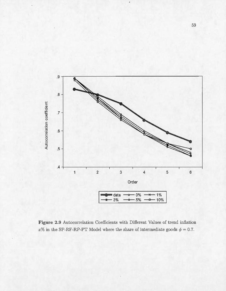
.8

ë Q) 'ü q:::

.7 '+--Q) 0 (.)

c .Q ...... ro .6 Q) L... L...

0 (.)

0 :5 <{ .5

2 3 4

Order

....- data ---o-- 0% ---w- 1% ---+- 3% -Ir- 5% -o--10%

59

5 6

Figure 2.9 Autocorrelation Coefficients with Different Values of trend inflation

x% in the SP-RF-RP-PT Madel where the share of intermediate goods cf;= 0.7.

CHAPTER III

FINANCIAL MARKETS A D THE CAPITAL ASSET PRICI G MODEL I A DSGE FRAMEWORK

Abstract

Thls paper aims at better assessing the interconnections between financial markets and

the real economy in a DSGE model calibrated to the U.S. economy. We incorporate

a fi nan cial markets sector based on geometrie Brownian motion ( GBM), alongside the

capital asset pricing model (CAPM) to account for households interventions on the stock

market. We show that consumption, output and investment react less to a technology

shock, whlle the nominal interest rate, inflation and labor are responding more stTOngly,

compared to the case where financial markets are ignored. Ivioreover, the negative effects

of a tightening monetary policy shock on output, consumption, inflation, investment and

labor are more significant. Finally, a positive financial markets shock exerts a downward

pressure on the nominal interest rate when the beta coefficient of the assets portfolio is

positive.

JEL classification: E44, E52, Gll , Gl2.

K eywords: CAPM; Stock markets; Monetary policy; Portfolio choice; GBM.

61

3.1 Introduction

The recent financial crisis has shawn how difficulties in financial markets

can turn into harmful consequences to the economy as a whole. It also revealed

the limits of traditional monetary policy tools in a context of t he zero lower bound

(ZLB) on nominal interest rates (see, e.g. , Coibion, Gorodnichenko and \iVieland,

2012; Aruoba and Schorfheide, 2013 ; Barthelemy and Marx, 2013; Gavin, Keen,

Richter and Throckmorton, 2013; Richter and Throckmorton, 2013). Therefore,

our work seeks to deepen the analysis of the intercom1ections between financial

markets and the real economy in DSGE models. This paper offers two main

contributions. First, it provides new findings on the impacts of technology and

monetary policy shocks for the economy in DSGE models where stock markets are

explicitly modelled. The dynamics of financial markets are described based on ge­

ometrie Brownian motion (GBM) , and the capital asset pricing madel (Hereafter,

CAPM) that is a madel of t he assets portfolio choice is introduced to account for

the behavior of households on the stock market in terms of purchases of risky as­

sets. Second, it shows how a financial markets shock affects the real economy. We

show that following the technology shock, the positive responses of consumption,

output and investment are lower in the CAPM madel than in the basic madel

where financial markets are ruled out. However, the decrease in the nominal in­

terest rate, inflation and labour is more important. In fact , a positive technology

shock is perceived by investors as an element that may increase the profits of firms ,

implying an increase in the expected return rate on risky assets . So, households

invest more in risky assets instead of consuming as anticipating higher future prof­

its of firms. This leads to a stronger decline in the nominal interest rate in the

CAPM madel since bonds are no longer attractive in that context. Therefore,

production, investment and employment decline. Moreover, the negative effects

of a tightening monetary policy shock on output , consumption, inflation, invest­

ment and labor are stronger in the CAPM madel than in the basic madel. A

contractionary moneta.ry policy shocl<: causes returns on securities to fall, because

financial markets anticipate a decline in the economie a.ctivity that could lower

future profits of firms. This ma.kes the decrease in such variables higher in the

62

CAP l model than in the basic model.

The second contribu tion of the paper is to assess the impact of a financial

markets shock on macroeconomie variables, especially its effects on the nominal

interest rate . The financial markets shock originating in the stock market is

meant to represent an exogenous increase in the return on the stock market.

It may result from an information in financial markets or in the economy as

a whole, which is perceived by investors as something that could hit the stock

market. Here, following a positive financial markets shock, returns on the stock

market and on securities increase while the nominal interest rate is falling when

the beta coefficient of the household assets portfolio is positive for any value of

the weight invested in risky assets. Consumption, output, inflation, investment

and labor increase due to the increase in expected gains made by households on

financial markets. Furthermore, the positive reactions of the return on securities,

consumption, output, inflation, investment and labour, and the negative response

of the nominal interest rate are more important for higher posit ive values of the

beta coefficient of the portfolio when the share of risky assets is constant. A

higher value of the beta coefficient is associated with higher expected returns on

the portfolio. vVe also find that t he positive reaction of the return on securities is

decrea..sing in the share of risky a..ssets in the portfolio while the negative response

of the nominal interest rate is increasing, for a constant beta coefficient of the

portfolio. A higher value of the share of risky assets means a more diversified

portfolio that is associated with low risk and return according to the CAPM

framework. Thus, the increase in consumption, output, inflation, investment and

labour is less large, since the anticipated profits here following the financial market

shock are lower. However, the nominal interest rate reacts positively for a negative

value of the beta coefficient, and then, consumption, output , inflation, investment

and labour decrease.

The key implication of these results for central banking in our model econ­

omy in the case where beta coefficient of the portfolio is positive is that, an upturn

in financial markets is expected to exert downward pressure on the nominal inter­

est rate for any positive beta coefficient of the household portfolio. It turns out

63

that , a rise in financial markets not accompanied by a reaction of the central bank

should rosult in lower nominal interest rates. T he monetary authority should then

increase the nominal interest rate following the posit ive financial markets shock

in arder t o bring dawn inflation on the one side. Conversely a decline in financial

markets gives rise t o an increase in the nominal interest rate . The cent ral bank

can then lower its policy rate to boost the economy. In short , the cent ral bank

should increase the nominal interest rate when finru1cial markets are in a strong

moment um of rising, and lower it when they are experiencing sharp declines.

Finally, we find that the CAPM model is successful in reproducing most of

the salient features of the U.S. economy, particularly, key macroeconomie volatil­

it ies, autocorrelations and correlations wit h output.

This paper relies on Kendall and Hill (1953) , Osborne (1959), Roberts

(1959) , Samuelson (1965), Black and Scholes (1973) , Barmish and Primbs (2011)

and Lochowski and Thagunna (2013) that focus on the modeling of the priee and

return of a stock by using GBM. But the peculiarity of t he paper is that we con­

sider here an application of GBM to the stock market index in order to highlight

the movements of the stock market as a whole. Then, household portfolio choice

decisions are taken into account following Markowitz (1959), Sharpe (1964), Lint­

ner (1965), Frun a (1996) , and Fama and French (2004) . According t o the CAPM,

individuals hold a portfolio that is a combination of risk-free assets (bonds) and a

single risky portfolio of securit ies available in the stock market . "The CAPM as­

sumes investors are risk averse and when choosing among port folios, they only care

about the mean and variance of their one-period investment retmn. As a rosult ,

investors choose "mean-variru1ce-efficient " port folios in the sense that portfolios i)

minimize t he variance of portfolio return given expected return and ii) maximize

expected return given variance" (see, FaJTia and French, 2004). Thus, the CAPM

enables us to highlight the trade-off between risky-free assets and risky assets in

portfolio allocation decisions of individuals. This allows to make the link between

financial markets and the real economy, part icularly through investment decisions

in stocks and bonds of t he representative household. However , unlike t he papers

cited above, the weights to be assigned to each type of asset in the portfolio are

64

the result of an optimization problem of t he representative household even if they

remain constant in the model. Furthermore, we assume t hat the risky portfolio is

contained in the market portfolio which is defined as the portfolio representing all

risky assets on the market. In other words, the risky portfolio consists of securit ies

belonging to the market portfolio but different from the latter.

The paper is also related to some works that incorporate risky assets in

DSGE models. For instance, De Paoli, Scott and Weeken (2010) investigate the

behavior of asset priees using a second-order approximation· to show how the risk­

free real interest rate, the return on equity, the equi ty premium and the real and

nominal term structure change with variations in sorne DSGE mode! parameters .

Fornero (2011) uses a consumption capital a.sset pricing model (C-CAPM) and

approximates it up to the third order to characterize the effects of various shocks

on real interest rates, the risk premium for different bonds maturities and the

term structure of interest rates. However, our paper stands out on some points.

We propose a formai modelling of the stock market in a DSGE mode! with the

CAPM to analyze especially the direct effects of a shock to the financial markets

on the overall economy. In addition, assets priees and returns are modelled using

GBM rather than approximation methods.

Finally, our mode! features a staggered priee setting mechanism and habit

formation as usual in DSGE models , and a positive trend inflation to reflect

the fact that the central bank inflation target is different from zero (see, Ascari ,

2004; Ascari and Ropele, 2007; Coibion and Gorodnichenko, 2011; Phaneuf and

Tchakondo, 2012 , 2013). Moreover the mode! is calibrated to the U.S. economy

and used to evaluate the impacts of standard supply and demand shocks and the

financial markets shock on macroeconomie variables , and thus, to make explicit

how financial markets are linked to the real economy.

The paper is organized as follows . Section 2 describes the mode!. Section 3

discusses the parameters calibration. Section 4 reports and discusses the results.

Section 5 concludes.

65

3.2 The 1\I.Iodel Econmny

The economy is populated by a lm·ge number of firms , each producing a

differentiated good indexed by j E [0 , 1]. We allow for a stock market where

households can purchase equities that are issued by firms . Finally, there is a

central bank conducting an endogenous monetary policy.

3.2.1 Firms: Optimal priee setting

Denote by Yt a composite of differentiated goods Yt(j) for j E [0 , 1] such

that Yt = [!~ Yt(j)CB- 1)1Bdj]0 f(1:1- 1), where (} E (1, oo) is the elasticity of substitution

between the goods. The composite good is produced in a perfectly competitive

aggregate sector.

The demand functions for good of type j resulting from optimizing behavior

in the aggregation sector is

(3.1)

where Pt is the priee of the composite good which is related to the priees Pt(j)

for j E [0, 1] of the differentiated goods and given by Pt= [JJ Pt(j)C1- 0)djjl1(1-o).

The production function for a good of type j is

(3.2)

where At is a technology shock assumed to follow a stationary AR(1) process,

Kt(j) and Lt(j) are the inputs of capital and labor.

Each firm acts as a price-taker in the input markets and as a monopolistic

competitor in the product market. A firm can choose the priee of its product ,

taking the demand schedule in (3.1) as given. Priees are set according to the

mechanism spelled out in Calvo (1983). In each period, a firm faces a constant

66

probability 1 - ~P of reoptimizing its pri_ce, with the ability to reoptimize being

independent across firms and time.

A firm j allowed to reset its priee at date t chooses a priee Pt(j) to ma:ximize

its profits oc

Et I)çpr-t Dt,T[Pt(j)Y;t(j)- v(Y;l(j))L (3.3) T=t

where E is an expectations operator, Dt.T is the priee of a dollar at time Tin units

of dollars at time t , and V(Yf(j)) is the nominal cost of producing Y7d(j) , which

is equal to VTYf(j), with VT denoting t he nominal marginal cost of production at

time T.

Solving the profit-maximization problem yields the following optimal pricing

decision rule:

( B ) [Et ~(Çpt-tDt,TyTd(j)VT ]

Pt(j) = - T-~ ) e- 1 Et L.(~p)T-tDt,TY/'(j)

T=t

(3.4)

which says the optimal priee is a constant markup over a weighted average of

marginal costs for the periods the priee will remain effective.

Sohing the firm's cost minimization problem yields the following nominal

marginal cost function:

VT = a-et(1- a) - (1-a)A_;:-1 (R~t' (1-VT)1-et ' (3.5)

where R~ is the nominal rentai rate on capital and WT is the aggregate nominal

wage rate. The real marginal cost is therefore expressed as

MCrT =Ci)= a-a(l - a)-(l-a)A_;:-1 (T;t (w7 )l-a , (3.6)

with r~ = R~/ P7 and wT = W7 / PT, indicating respectively the real rental rate on

capital and t he real wage rate. Consequently, the optimal pricing equation (3.4)

becomes

67

( e ) [Et ~(~Py-tDt,r PlYr(ITt+l x IIt+2 x .. . x IIr )

81\1Crr1

Pt(j) = el T~ '

- Et 2:(~v )r-tDt ,rpt- 1 Yr(IIt+ 1 x Ilt+2 x ... x IIr) 8- 1

r=t (3.7)

where Î = IIr = Pr/ Pr _1 for T = t + 1, t + 2, ... , t + oo, with Î ~ 1 reflecting

trend inflation, and II-r the gross inflation rat e at time T . Following Ascari (2004) ,

Ascari and Ropele (2007) and Phaneuf and T chakondo (2012, 2013) we allow for

positive trend inflation to reflect the fact that the inflation target of the central

bank is different from zero.

A firm that does not reset its priee in a given period , nonetheless chooses

the inputs of capital and labor that minimize production cost.

3.2.2 Households: Portfolio choice decisions

The representative household 's preferences are described by the expected

ut ility function:

oc { LI+x} Et L /3t log( Ct - hCt-1 ) - 'r!-1

_t - , t=O + X

(3. 8)

where f3 E (0 , 1) denotes the subjective discount f~ctor , h E (0 1) is a habit

formation parameter , 'Tl measures the weight on leisure in the ut ility function, and

x is the inverse of the Frisch wago elasticity of labour supply. Ct and Ct_1 are

CUITent and past-period consumpt ions of household, and L t is t he labor.

The budget constraint in nominal terms that household faces at time t is

given by the following relation:

Rfec Pt[ Ct + ft] + Bt + S:C ~ ltVtLt + R; Kt + RtBt-1 + ~s:~1 + ÎÏt +Tt, (3.9)

where, s;c represents a set of securit ies or different risky assets that are especially

equities issued by firms on the stock market. s;c is assumed to be different from

68

the market index, since we rule out t he possibility for the representative household

to instant ly buy all t he securit ies available on t he stock market .

The household enters period t wit h a port folio of total assets composed of

nominal bonds Bt_ 1 and nominal securities Sf:_1 . Bonds pay t he gross nominal

interest rate Rt set by central bank and considered here as t he risk-free rate, and

securit ies pay t he expected gross nominal interest rate Et(Rf~~) referred to as the

expected rate of the return on securit ies. :Et is int roduced to allow for risk-return

differences between bath types of assets in equilibrium.

Meanwhile, Wt is t he nominal wage rate for labor Lt, R~ is t he nominal

rental rate on capital, Ilt is household 's dividends received for t he ownership of

firms, and Tt indicates a lump-sum transfer the household gets from the govern­

ment.

The physical capital accumulation equation is given by

K t+l = (1 - o) Kt + [ 1- S ( f:~ 1 )] ft, (3.10)

where (j is t he physical capital depreciation rate, ft denotes t ime t purchases of

investment goods. The term S ( 1:~ 1 ) is a convex investment adjustment cast

function. It is a..c;sumed that in the steady state S (1) = S' (1) = 0, and "' =

S" ( 1) > 0 indicates the investment adjustment cast parameter.

The household acts as a price-taker in bath goods and financial markets.

The representative household chooses consumption Ct , hours worked Lt, bonds Bt ,

securities St, the physical stock of capital for the next period K t+1 and investment

ft that maximize (3 .8) subj ect to (3 .9), (3.10) and a no-Ponzi-game condit~on . 1

The first-order condit ions for this optimization problem are :

(3.11)

1. Following Alstadheim and Henderson (2006) , this condit ion could be: r (B Tik=t-1 R-1 +sec Tik= t-1 (Rs•• )-1 ) > 0 ·t l Tik=-1 R -1 t!! t k=O k t k=O k ' Wl 1 k= O k 1, and

Tik= -1 (Rs•• ) - 1 = 1 k=O k - ·

À = (3 E (Rf~~ Àt+l ) t t " ' L.Jt+l

ÀtPt =(Ct- hCt- 1)- 1- hf3 Et(Ct+l - hCt)-1,

ÀtPt = (3Et[Àt+l(~+1 + (1- 6)Pt+l)],

69

(3.12)

(3.13)

(3.14)

rJL~ = Àt liVt, (3.15)

Pt[ Ct+ I<t+l- (1- 8)I<t] + Bt + s:c = vVtLt + R~ K t+ RtBt-l + ~:c s:~ 1 + ÎÏt +Tt,

(3.16)

where Àt is the Lagr angian multiplier associated with the budget constraint. From

(3.11) and (3.12), we obtain in equilibrium a relation between the expected rate

of return on securities (E(Rf c)) and the risk-free rate (Rt) that is:

s ec Et(~+ 1 ) = RtE(I:t+l)· (3.17)

Here, ~t can be interpreted as a nominal gross spread rate between R fc and Rt

expressed proportionally to the risk-free rate, and allowing for di:ff:"erences in ter ms

of returns between bonds and securities.

Therefore, the weight invested by the household in risky assets proportion­

ally to total assets wp = s;~~Bt, and 1 - wp = s;!~Bt is the weight invested in

the risk-free asset. So, from the portfolio theory 2 , the expected return on the

household portfolio of assets is given by

Et (Rpt+ 1 ) = wpEt (Rf~~)+ (1- wp) Rt . (3.18)

Wp is one of the key elements of the model in the sense that it determines house­

hold portfolio choice decisions: t he higher is Wp , the more household invests in

additional different risky assets 3 .

2. The portfolio t heory informs about investment decision making. It focus among others

on the formation of an optimal portfolio of assets , particularly the determination of the best

risk-return opport unities from feasible investment portfolios and the choice of t he best portfolio

from that fea .. 'lible set (sce, e.g. , Bodie ct al. , 2005, ch. 5-6).

3. The assumption that the increase in wp is associated with t he integration of additional

assets in portfolio, is necessary here to take in account the concept of portfolio diversification:

the more diversified is the port folio , the less risky it is.

70

3.2.3 Financial markets: The CAPM

\lYe suppose a financial sector that is only composed of financial markets

mainly a stock market, ruling out the possibility to have a banking system in the

model economy. At time t, the household 2 can purchase securities Sfc that are

firms equities issued on the stock market.

Following Kendall and Hill (1953), Roberts (1959), Osborne (1959), Samuel­

son (1965) Black and Scholes (1973) , Barmish and Primbs (2011) and Lochowski

and Thagunna (2013) , we assume that the aggregate stock market priee s;n, which

can be considered here as the stock market index is governed by the geometrie

Brownian motion: dsrl sm = 11dt + O"dBrt , (3.19)

t

where fJ, is a constant rate of return often called the drift and captures the an-

nualized expected return of the stock market , O" is the volatility representing the

annualized standard deviation a.c;sociated with the underlying process, and Brt

is the Brownian or \lViener process. 4 This equation is viewed as a stochastic

differentiai equation because the stock market priee s;n is defined implicitly by

describing its changes through time random effects. Thus, the analytical solution

of (3.19) is given by

S;'~ = s~nexp { (11 - ~2

) t + O" Brt } ,

where S0 > 0 is the initial value or the stock priee at time O.

(3.20)

The gross return of the stock market , R;_n = log (S;n / 3';::._1) , derived fTom

(3.20) becomes

(3.21)

4. A Brownian motion process Brt , t 2:: 0, is a continuous stochastic process with the

following properties: (i) it starts at zero, i.e. Br0 = 0; (ii) it has independent increments; (iii)

for every t > s 2:: 0 Br·t- Br5 has a normal distribution N(O , t- s), (see, e.g., Lochowski and

Thagunna, 2013; Ermogenous, 2005).

71

where fR[" is assumed to be a stock market shock following a stationary AR(1)

process. éRt" could capture phenomena that are missing in the geometrie Brownian

motion (3.19) such as jumps in the stock market , particularly during a financial

markets turmoil.

To see how household portfolio choice decisions and the stock market inter­

play, we resort to the CAPM (see, e.g. , Markowitz, 1959; Sharpe, 1964; Lintner,

1965· Fama, 1996; and Fama and French, 2004) that establishes a relationship

between the expected performance of the household portfolio of assets Et ( Rp,+1 ),

and the stock market return Et (R;+1) such that:

(3.22)

where f3p called the beta coefficient of the portfolio reveals the way and the extent

to which returns on the portfolio and the market move together . This CAPM

equation suggests that the expected return on the household portfolio Et ( Rpt+1 )

is the risk-free rate Rt , plus a risk premium, which is the portfolio beta coefficient

f3p, times the premium per unit of beta risk E (R~~ 1 ) - Rt.

Formally, the beta of the household portfolio f3 p is defined as the covariance

of its return with the market return divided by the variance of the market return

(see, Fama and French, 2004),

(3.23)

So, the equation (3.22) becomes

E (R ) = R Cov(Rp,Rm) [E (pm ) - PJ Pt+ l t + 2 _."t+ l 1.11. '

ŒR"' (3.24)

with the ratio Cov(Rp,R"'), i.e. , f3p measuring the sensitivity of the return on the OR'n

household portfolio to variations in the mru·ket return.

From the household portfolio decision in (3 .18) , the variance ofthe portfolio

is given by Œ~P = w~Œ~sec' where Œ~sec indicates the mean of the variance of risky

assets. This implies that (3.23) becomes

(3.25)

72

where P(Rp,Rm) is the correlation coefficient between returns on the portfolio and

the market.

In other words, {Jp is the (implicit) measure of the household portfolio risk and

appears a..c:; another key element of the model, sin ce one can infer from {3 p important

features of the household portfolio. In fact , the sign and magnitude of {Jp depend

on the type of risky assets that household wants to have in its portfolio. For

instance, {3 p = 0 means that the return on the household portfolio is insensitive

to stock market fluctuations , implying that the portfolio of assets consists only of

risk-free assets. \rVhen {Jp = 1, the portfolio performance is exactly the same as

the market. This suggests either that the household buys the stock market index

or a portfolio that replicates perfectly the market . For 0 < {3 p < 1, portfolio

and market returns evolve together but the portfolio weakly reacts to market

fluctuations unlike the case where the portfolio reacts strongly when {Jp > 1.

Finally, when {Jp < 0, portfolio and market returns move in opposite directions.

This can be the case when the representative household wants to take a reverse

position on the market , for example via a cali or a put. 5 In sum, by affecting

household investment decisions, {Jp and Wp also influence household consumption

choices. Therefore, they could be considered as factors linking financial markets

and the real economy and playing an important role in the transmission of shocks

from financial markets to the real economy and vice versa.

Another way to analyze the interconnections between financial markets and

investment and consumption decisions of the representative household can be

understood from (3.18) and (3.22) , by the following relation:

(3.26)

This relation suggests that the risk premium of the portfolio is equivalent to

the spread between the mean rate on securities and the risk-free rate, times the

weight invested in risky assets. The distinctive characteristic of (3.26) is that

i t highlights a relation between fin an cial market fe at ures ( ~m , Rr c, {3 p) the

5. A cali option/a put option, is the right to buy/to sel! an asset at a specified exercise

priee on or hefore a specified expiration date (see, e.g., Bodie et al. , 2005, Glossary).

73

household decisions (wp) and the monetary policy instrument (Rt).

Meanwhile, the equations (3.26) and (3.17) give rise to:

E(êt+I) = {3p [E (R;;~1 ) - Rt]' Wp Rt

(3.27)

where E(êt+I) = (1 - E(I:t+1)), denotes the expected nominal net spread rate

between E(Rfc) and R t. Thus, t he expected net spread rate is increasing in the

risk premium {3p [E(~~1 ) - Rt], since an increase in the risk premium implies

a strong contribution of risky assets to returns on the portfolio. However, the

net spread rate is decreasing in the weight invested in risky assets, Wp. In fact,

an increase of wp means according to the model an increased diversification of

the portfolio of risky assets. Therefore, the higher the portfolio of risky assets is

diversified, the lower are its return E(.Rf~~) and the net spread rate.

Moreover , one can derive from (3.26) the following equation:

)

Wp (3.28)

suggesting that the relation between stock market returns and secmities returns

depends on the sign of the beta coefficient of the portfolio. They move together

for {3p > 0 but conversely when {3p < O.

"V\T~ obta.in from (3.18) a negative relation between returns on securities and the

risk-free rate such that:

Wp

1-wp where Wp =/=- 1, (3.29)

implying that bonds become less attractive when returns on risky assets increase.

Finally, based on the equations (3.28) and (3.29), the relation between the risk-free

rate and stock market returns is given by

{3p

1-wp where Wp =/=-1 ,- (3.30)

showing as in (3.29) that bonds become less attractive when stock market returns

mcrease.

74

Therefore, t he equations (3.28) , (3 .29) and (3.30) may help to capture how .

financial markets shocks impact on the real economy, through t heir influence on

the monetary policy instrument and on households consumpt ion and investment

decisions in bonds and securities . On the other hand , they appear to be useful in

analyzing the effects of a monetary policy shock, in an economy where we take in

account the possibility for the household to acquire risky assets .

3.2.4 Cent ral bank

We assume that the central bank systematically reacts to deviations of infla­

t ion, Ilt , and out put grü\vth, Gyu from their steady-st ate values while smoothing

short-term movements in the policy rate, Rt (see also Erceg and Levin, 2003; Gali

and Rabanal, 2004; Liu and Phaneuf, 2007; El Omari and Phaneuf, 2011). Thus,

monetary policy evolves according to the following Taylor-type policy rule:

log(Rt, j R ) = Prlog(Rt- d R ) + (1 - Pr) [p1r log(IItfii ) + py log( GytjGy )] + tRp

(3. 31)

where Gyt = Yt/ Yt- 1 ; R , II , and Gy are the steady-state values of Rt, Ilt, and

GYt., respectively; and ER, is a monetary policy shock normally distributed wit h

zero mean and standard deviation Œ R·

3.2.5 Markets clearing conditions

Market clearing on capital and labor markets requires respectively

1

Kt = f K f( j )dj , 0

1

Lt = f Lf (j) dj. 0

The resource constraint of the economy implies t hat

(3.32)

(3. 33)

(3 .34)

Finally bonds and securit ies held by households are equal t o zero so Bt = 0

and s:c = 1 in equilibrium.

75

3.3 Calibration

We calibrate the model parameters to match salient features of the U.S.

economy. 6 Table 3.1 reports calibration values. We set the subjective discount

factor f3 to 0.9926, implying an annual real interest rate at the steady-state of

3%. The parameter Tf , denoting the weight on leisure in the utility function is

set equal to 1.315 (Christensen and Dib, 2008), so that the household spends

around one third of its t ime in market activities. The inverse of the Frisch wage

elasticity of labor supply x is assigned the value of 1 (Dib, 2010; Falagiarda,

2013), implying an elasticity of intertemporal substitution of labor of 1. The

depreciation rate of capital 6 is calibrated to 0.025 (Christiano, Eichenbaum and

Evans, 2005; Falagiarda, 2013) which implies an ammal rate of depreciation on

capital equal to 10%. We set the parameter of habit formation h to 0.8 (Fuhrer,

2000; Boldrin, Christiano and Fisher , 2001 ; Phaneuf and Tchakondo, 2013). The

AR(1 ) coefficient of the productivity process Pa is set at 0.95, and its standard

deviation CJa is set at 0.45 (Smets and vVouters, 2007) . The capital share in

aggregate output production a is set at 0.33 (see, Ascari, 2004; Dib, 2010) . The

steady-state gross inflation rate 1 is set equal to 1.0079 (see, Christensen and Dib,

2008).

The elasticity of substitution between differentiated goods e determines the

steady-state markup of priees over marginal cost, with a markup of e / ( e - 1) .

Rotemberg and Woodford (1997) assume a value-added markup of 1.2, implying

e = 6. Christiano, Eichenbaum and Evans (2005) estimate value-added markup at

1.2 in a model controlling for variable capital utilization. Nakamura and Steinsson

(2010) assume e = 4 and a value-added markup 1.33 in a menu-cost model. So,

we set e = 6, inducing a value-added markup of 1.2.

The parameter Çp, which measures t he probability of priee non-reoptimization,

is fixed as follows. In a sur·vey of postwar evidence on U. S. priee behavior, Taylor

(1999) documents that priees have changed about once a year on average. Using

6. See Appendi..x for detailed description of the dataset.

----- -------·- -- ----------- ----- -- - -

76

summary statistics from the Consumer Priee Index micro data. compiled by t he

U.S. Bureau of Labor Sta.tistics for 350 categories of consumer goods and ser­

vices, Bils and Klenow (2004) document that the median waiting time between

priee a.djustments has been 4.3 months when priee adjustments occuring during

temporary sales are taken into account , while it has been 5.5 months when they ·

are not . Their evidence, however, covers only a very short period of time, the years

1995-1997. Using a fewer categories of consumer goods and services, they report

evidence suggesting that for the longer period 1959-2000 the frequency of priee

adjustments is much lower than for the years 1995-1997. Nakamura and Steinsson

(2008) provide estimates of the frequency of priee changes ranging from 8 to 11

months when product substitutions and temporary sales are bath excluded, and

from 7 and 9 months when only temporary sales are excluded.

In light of these studies, we set the value of ~P at 2/3 (see also Phaneuf and

Tcha.kondo, 2012, 2013; El Oma.ri and Pha.neuf, 2011). Bils and Klenow (2004)

emphasize the median as their measure of waiting t ime between priee adjustments.

Approximating the waiting time to the next priee change by ~t, the median wa.iting

time between priee changes is given by -ln(2)/ ln(~p)· 7 Setting ~P = 2/3 implies

that the median waiting t ime between priee changes is 5.1 months, which is in t he

range of admissible values from micro level evidence.

The coefficients of the Taylor rule are ca.librated as follows: Pr = 0.8, p.,. = 1.5 and py = 0.125. These values are broa.dly consistent with recent estimates

reported in Smets and vVouters (2007) and Justiniano and Primeceri (2008) , and

with the calibration in Christiano, Eichenbaum and Evans (2005) and El Omari

and Phaneuf (2011) . The standard deviation of the monetary policy shock O"R is

set at 0.0004 (Ireland, 2007).

The calibration of the parameters rela.ted to financial markets is very tricky

as the existing literature is uninformative. So, we set t he volatility of stock market

O" to 0.017, which corresponds to the quarterly mean of the volatility of stock priee

7. See Cogley and Sbordone (2008, footnote 19).

77

index for U.S.(1977Q1- 2010Q1), i.e., the 360-day standard deviation of the return

on the national stock market index (Bloomberg). The market return rate p, is set

at 0.03 , which is equivalent to the mean value of the market return rate using

quarterly data on SP500 (1980Q1 - 2013Q1). Using quarterly data from Fama­

French benchmark factors returns (1930Q1- 2014Q2) , we set the beta coefficient

of the portfolio f3p at 3.3 which corresponds to the mean value. For the weight

invested in risky a..ssets Wp, we use a dataset from financial accounts of the United

States for the period 1950Q1-2014Q3 8 . Based on households treasury securit ies

and corporate securities, we obtain a mean value of 0.9 for the weight invested

in risky assets. Adding households savings deposits gives a mean value of 0.6

for the period which we set as a reasonable value of Wp. Further, a sensitivity

analysis is made with respect to sorne other values of f3p (-6, 5.5) and wp (0.4).

Finally, we approximate the stock market shock to a sentiment shock, which

refiects household beliefs about fluctuations in stock market bubbles (see Miao,

Vlang and Xu; 2012). Accordingly, we set the autocorrelation coefficient of the

stock market process PRm at 0.87 and its standard deviation CJR"' at 0.21.

3.4 Results

This section presents the results of the simulated madel. On the one side,

we present the effects of standard supply and demand shocks on sorne key macroe­

conomie variables. On the other side, we report their dynamic responses to the

financial markets shock. Figures 3.1 and 3.2 show the impulse responses functions

to technology and monetary policy shocks, respectively. Figures 3.3- 3.6 plot the

responses to the financial markets shock under various aspects.

3.4.1 Responses to technology shock

Figure 3.1 shows the impulse responses to a positive technology shock. Fol­

lowing this shock, in the basic madel , output and consumption are increasing while

8. See Appendix A, for more details.

78

inflation and nominal interest rate decline. For the CAPM, it must be stressed

that technology shock is perceived by financial markets as an element that may

increase the profits of firms. Thus, the expected return on securities increases in

reaction to the shock. This leads to a stronger decline in the nominal interest

rate in the CAPM model since bonds are no longer attractive in that context. So,

the increase in consumption, output and investment is lower in the CAPM model,

because households invest in risky assets as anticipating higher future profits of

firms. Therefore, compared to the basic model, the decline in inflation and labour

is stronger in the CAP1vl madel.

3.4.2 Responses to monetary policy shock

Figure 3.2 depicts the impulse responses to a contractionary monetary pol­

icy shock. In reaction to this shock, the nominal interest rate increases and output,

consumption, inflation, investment and labor fall on impact . Following a tight­

ening in monetary policy, returns on securities fall, since investors anticipate the

conditions of economie activity that could limit future profits of firrns. So, the

decrease in such variables is higher in the CAPM model than in the basic model.

3.4.3 Responses to financial market shock

In what follows , we show the impulse responses to a positive financial mar­

kets shock. This financial markets shock can be interpreted as an exogenous

increase in the return on the stock market. It may result from an information

in financial markets or in the economy as a whole, which is anticipated or per­

ceived by investors as something that could hit the stock market. The analysis is

undergone through a series of cases. Basically, the purpose of this analysis is to

understand how a financial markets shock could affect macroeconomie variables

especially its effects on the monetary policy instrument in our madel economy.

s ec

Case 1. For any (3p > 0, Wp being constant, 88R~m > 0 and %fit~, < O. There

exists a positive relation between R;n and Rf c, and a negative relation between

79

~n and Rt.

So, a positive financial markets shock, by increasing the return on the stock

market induces the return on securities to increase as showed in Figure 3.3. House­

holds could invest more to take advantage from higher future returns on risky

assets. However, the return on bonds is expected to decrease as they become

relatively Jess attractive for investors. Thus, the rise of future anticipated gains

on risky assets combined with low bond yields should result in an increase in

consumption, output, inflation, investment and labour in reaction to the financial

markets shock.

. ôRfec ôRrc Case 2. Let j3 p > 0, w p be~ng constant. For /3 p 1 > f3 p 2 , ôR(" (/3 P1 ) > ôfiem (/3 P2)

and 1 Î}if. (/3 P 1 ) 1 > 1 %Ji;, (/3 P2 ) 1· The pos-itive relation between R": and Rfc, and

the negative relation between ~m and Rt are increasing in f3p .

This proposition can be seen as a corollary of Case 1. , since we have the

same responses of our variables of interest following a financial markets shock.

However, the analysis is undergone taking different values of f3p. Figure 3.4 shows

that, the positive reaction of the return on securities and the negative response of

the nominal interest rate to the financial markets shock are increasing in f3p for a

fix weight invested in risky assets wp . In addit ion, the increase in consumption,

output, inflation, investment and labour is more important for higher values of f3p.

In fact , as f3p positively affects the expected return on the household portfolio of

assets , higher profits are associated with higher value of f3p. This leads to a rela­

tive large increase in such macroeconomie variables in the ca..se where f3p is higher.

. aRre ôR?ec Case 3. Let f3p > 0 bezng constant. For Wp1 > Wp2 , ôRm (wpJ < ôR"' (wp2 )

t t

and 1 %/if. (wpJ 1 > 1 %Ji;. (wp2 ) 1 · The positive relation between Rr~ and Rte ~s decreasing in w p , wh ile the negative relation between R~n and Rt is increasing.

Here again, we deal with a corollary of Case 1. , but for different values of

wp, f3p being constant. The positive reaction of the return on securities to the

financial markets shock is decreasing in wp, while the negative response of the

-- - - ----- - ------ ------ ------ -- - - ------ --- --- --------------

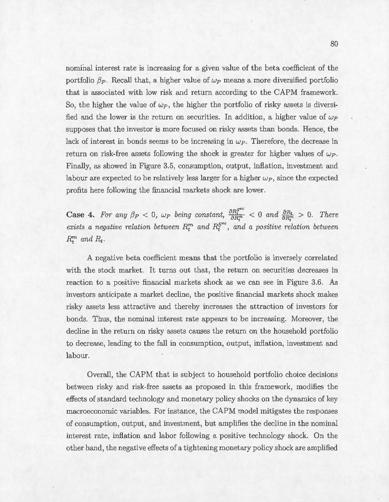
80

nominal interest rate is increasing for a given value of the beta coefficient of the

portfolio f3p. Recall that , a higher value of W p means a more diversified portfolio

that is associated with low risk and return according to the CAPM framework.

So, t he higher the value of wp, the higher the portfolio of risky a..c;sets is diversi­

fied and the lower is the return on securit ies. In addition, a higher value of wp

supposes that the investor is more focused on risky assets than bonds. Renee, the

lack of interest in bonds seems to be increa..c;ing in wp. T herefore, the decrease in

return on risk-free assets following the shock is greater for higher values of wp.

Finally, as showed in Figure 3.5, consumption, output, inflation, investment and

labour are expected to be relatively less larger for a higher w p , since the expected

profi ts here following the financial markets shock are lower .

' sec Case 4. For any f3 p < 0, wp being constant, 8~"" < 0 and g:,~, > O. There

t t

exists a negative relation between R7~ and Rfec, and a positive relation between

R~n and Rt,.

A negative beta coefficient means that the portfolio is inversely correlated

with the stock market. It t urns out that , the return on securities decrea..c;es in

reaction to a positive financial markets shock as we can see in Figure 3.6. As

investors anticipate a market decline, the positive financial markets shock makes

risky assets less attractive and thereby increases the attraction of investors for

bonds. Thus, the nominal interest rate appears to be increasing. Moreover , the

decline in the return on risky assets causes the return on the household portfolio

to decrease, leading to the fall in consumpt ion, output , inflation, investment and

labour.

Overall , the CAPM that is subject to household portfolio choice decisions

between risky and risk-free assets as proposed in this framework, modifies the

effects of standard technology and monetary policy shocks on the dynamics of key

macroeconomie variables. For instance, the CAPM model mitigates the responses

of consumption, output , and investment, but amplifies the decline in t he nominal

interest rate, inflation and labor following a posit ive technology shock. On the

other hand, the negative effects of a t ightening monetary policy shock are amplified

81

since the responses of output, consumption, inflation, investment and labor are

stronger in the CAPM model than in the basic model.

In addition, a positive financial markets shock has different effects on the

monetary policy instrument depending on values taken by the beta coefficient

of the household portfolio {3p, and the weigh invested in risky assets wp . In

particular, Cases 1.,2.,3. show a negative reaction in the nominal interest rate

to the financial markets shock when {3p is posit ive for any value of omega. Here,

consumption, output, inflation, investment and labor react positively. However,

the nominal interest rate responds posit ively to the shock from Case 4. , where

{3p is negative and consumption, output inflation, investment and labor decrease.

From the monetary policy perspective, Cases 1. ,2.,3. suggest that an upturn

in financial markets is expected to exert a downward pressure on the monetary

policy instrument in our model economy. It turns out that, a rise in financial

markets not accompanied by a reaction of the central bank may result in lower

nominal interest rates. The monetary authority should then increase the nominal

interest rate following the positive financial markets shock in order to bring down

inflation. Conversely, a decline in financial markets gives rise to an increase in the

nominal interest rate. The central bank can then lower its policy rate to boost

the economy. In short , the central bank should increase the nominal interest rate

when financial markets are in a strong momentum of rising and lower it when

they are experiencing sharp declines.

As a consequence, these results suggest that financial markets, particularly

stock markets might deserve special attention from policy-makers and researchers

when they a..ssess the ins and outs of monetary policy.

3.4.4 Volatilities and autocorrelations

Here, we assess the capacity of the CAPM model t hat accounts for house­

holds' assets portfolio choice decisions to replicate sorne important features of the

U.S. macroeconomie fluctuations. As in Christensen and Dib (2008) , and Dib

(2010) , we pay attention to the model-implied volatilities (standard deviations) ,

82

relative volatilities , and correlations of output with sorne key variables. Table

3.2 reports the standard deviations and relative volatilities of output, consump­

tion, investment, la bor, and inflation from the data, and for the two simulated

models. 9 The standard deviations are expressed in percentage terms. The model­

implied standard deviations relatives volatilities and unconditional correlations

with output are calculated using technology and monetary shocks.

Column 3, in Table 3.2 displays standard deviations, relative volatilities,

and unconditional autocorrelations of the actual data for the period 1954Ql-

2008Q3. Colwnns 4 and 5 however, report those simulated with the basic and

CAPM models, respectively. In the data, the standard deviation of output is

1.54, consumption 1.22, and investment 7.08. Labour has a standard deviation

of 1.76. Inflation is less volatile with a standard deviation of 0.38. In addition,

investment and labor are 4.60 and 1.14 times as volatile as output, while consump­

tion and inflation are less volatile than output, with relative volatilities of O. 79

and 0.25 respectively. In addition, output, consumption, investment and labor

are highly persistent, with autocorrelations coefficients that are, at least, equal to

0.8; inflation is less so, with a coefficient of 0.44.

The simulation results show that, in the CAPM madel, all volatilities are

close to those in the data. However, the basic madel, in which the financial market

sector is absent, overpredicts all the volatilities. Compared to the basic madel ,

the CAPM madel is also successful at matching the relative volatility of most of

the variables. Mm·eover , the CAPM madel does a better job at matching the

autocorrelations shawn in the data.

Finally, Table 3.3 displays the cross-correlations of the data and those sim­

ulated in the two models. Overall, the correlations of output with consumption,

investment, labor, and inflation implied by the CAPM madel fit better those

observed in the data.

9. Ail series in the data are HP-filtered before calculating their standard deviations as

weil as their unconditional autocorrelations a.nd cross-correlations

83

3.5 Conclusion

The aim of this paper is to improve our understanding of the interrelations

between financial markets and the real economy . . Vve propose a DSGE frame­

work that embeds a financial markets sector based on geometrie Brownian mo­

tion (GBM) to describe stock markets priees and returns. We also incorporate

the capital asset pricing mo del ( CAPM) to account for the behaviour of investors

on stocks markets in tenns of purchases of equi ties. The contributions of this

paper are twofold. First, following a technology shock, consumption, output and

investment respond less here, while inflation and labor are reacting more strongly

than the baseline model where financial markets are ruled out. In addition, the

negative effects of a tightening monetary policy shock on output , consumption,

inflation, investment and labor are more significant. Second, a positive financial

markets shock negatively affects the nominal interest rate when the beta coeffi­

cient of the household portfolio of assets is positive. In that situation, a lack of

reaction of the central bank may result in a downward pressure on the nominal

interest rate . Accordingly, our results suggest that stock markets might deserve

special attention from policy makers and researchers when they analyze the ins

and outs of monetary policy.

We acknowledge the model developed here suffers the limitations and short­

comings associated with the basic CAPM that is one of the main pillars of our

framework. Thus, further works could extend the analysis by talüng account of

the three-factor model for expected returns proposed by Fama and French (1993,

1996, 2004). Doing so may quantitatively affect sorne of our results, but the

int uition developed here will still remain in force.

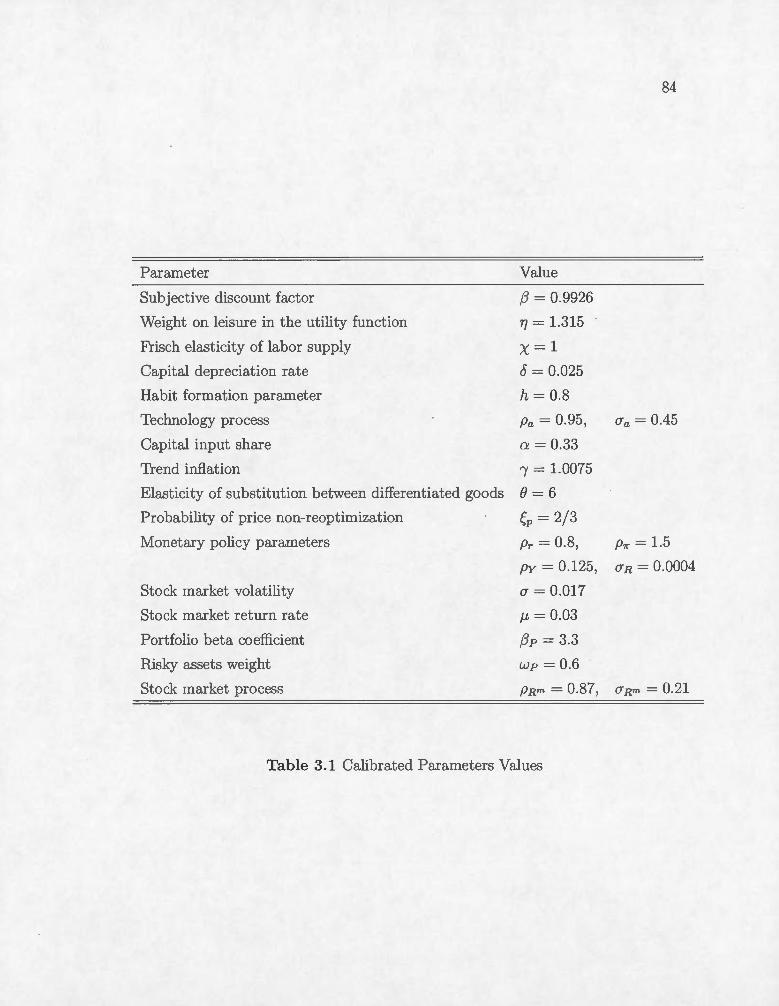
Parame ter

Subjective discount factor

Weight on leisure in the utility function

Frisch elasticity of labor supply

Capital depreciation rate

Habit formation parameter

Technology process

Capital input share

Trend inflation

Elasticity of substitution between differentiated goods

Probability of priee non-reoptimization

Monetary policy parameters

Stock market volatility

Stock market ret urn rate

Portfolio beta coefficient

Risky assets weight

Stock market process

Value

f3 = 0.9926

rJ = 1.315

x= 1 8 = 0.025

h = 0.8

Pa= 0.95 ,

a= 0.33

1 = 1.0075

B=6 f,p = 2/3

Pr = 0.8,

py = 0.125,

CT= 0.017

fJ- = 0.03

f3 p = 3.3

Wp = 0.6

PRm = 0.87,

Table 3.1 Calibrated Parameters Values

84

CTa = 0.45

p7f = 1.5

CTR = 0.0004

CTR"' = 0.21

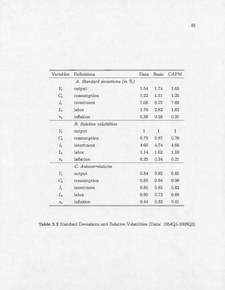
85

Variables Definitions Data Basic CAPM A. Standard deviations (in %)

Yt output 1.54 1.74 1.65

Ct consumpt ion 1.22 1.51 1.25

I t i.nvestment 7.08 8.25 7.69

Lt la bor 1.76 2.82 1.82

1ft inflation 0.38 0.59 0.35

B. Relative volatilities

Yt output 1 1 1

Ct consumption 0.79 0.87 0.76

I t i.nvestment 4.60 4.74 4.66

L t la bor 1.14 1.62 1.10

1ft inflation 0.25 0.34 0.21

C. A utocorrelations

Yt output 0.84 0.92 0.85

Ct consumption 0.85 0.94 0.90

I t investment 0.80 0.85 0.82

L t la bor 0.90 0.73 0.88

1ft inflation 0.44 0.33 0.41

Table 3.2 Standard Deviat ions and Relative Volatilities (Data: 1954Q1-2008Q3)

86

Variables Definitions Data Basic CAPM

yt output 1 1 1

Ct consumption 0.87 0.16 0.84

ft investment 0.91 0.73 0.82

Lt la bor 0.87 0.88 0.86

1rt inflation 0.15 0.89 0.20

Table 3.3 Correlations with output (Data: 1954Q1-2008Q3)

87

Output Consumption

:::E.-------1 0 5 10 15 20

~E'--- -~~'·'·~- -:- --J :r-'--- ~·~,~~:·_--- - ~ 0 5 1 0 15 20 0 5 1 0 15 20

lnvestment Labor

_:F _ _ _ _ ; ; j 0

0

o:E ___ :-- _____ j 0 5 1 0 15 20 0 5 1 0 15 20

~-Basic 1

--- CAPM

Figure 3.1 IRFs to a Positive Technology Shock for (3p = 3.3 and wp = 0.6.

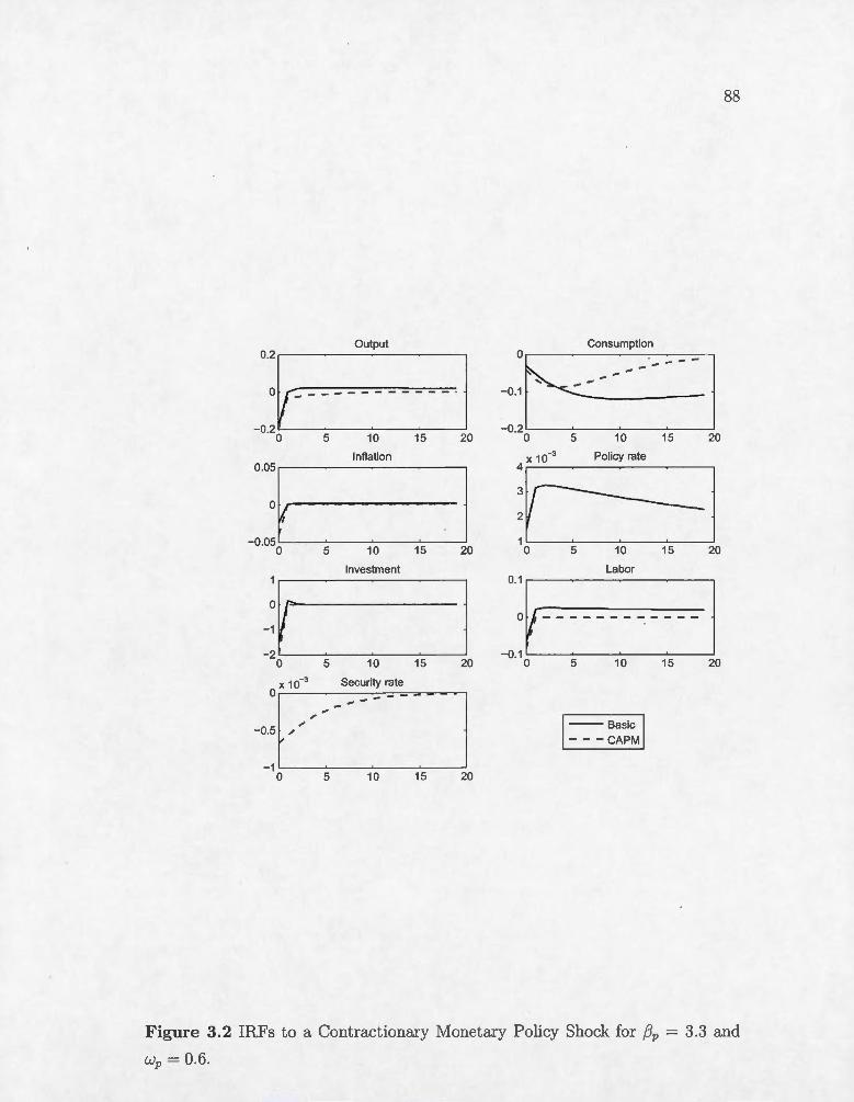
88

_::Vi--- -~t~"t_ --- l :::E~~•:m:t:"_---] 0 5 1 0 15 20 0 5 1 0 15 20

_:J ; lofl•tioo ~ l ~Ë 1

0 5 10 15 20 0 5 10 15 20

lnvestment Labor

:t : : : l -~+- u - - -:- - u - -1 0 5 1 0 15 20 0 5 1 0 15 20

-J ~o,' , _ :~~,,~ ~t~ ~ _ l ~-Basic 1

--- CAPM

0 5 10 15 20

Figure 3.2 IRFs to a Contractionary Monetary Policy Shock for /3p = 3.3 and

Wp = 0.6.

l'~ : Ootp"t :

1

~E:: 1

0 5 1 0 15 20 0 5 1 0 15 20

I~ : ''''"'" : 1 :~b2: l 0 5 1 0 15 20 0 5 1 0 15 20

~~~ : '""tmoot :

1

:;[L.J.-.-o-

1

L•b--.Jor

0.01

0 5 10 15 20 0 5

Market rate

0.04

0.02

10 15 20

0 .015~

0.005

oL---~--~~~==----~

0.06~Secumy rate

oL---~----~~~~--~ 0 5 10 15 20 0 5 10 15 20

1-- CAPM with I3P = 3.3 1

89

Figure 3.3 IRFs to a Positive Financial Market Shock for j3P > 1 and wp = 0.6 .

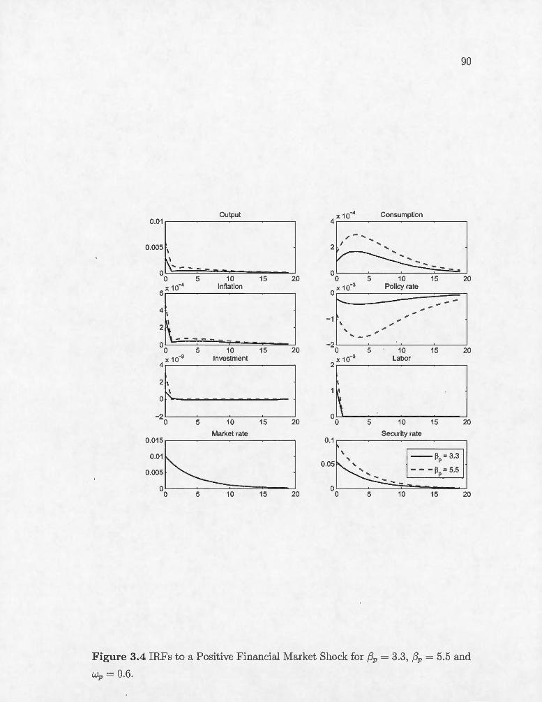
15 20

90

x 10-4 Consumption 4.-----------------~----.

/

2 1

-1 \

' 0 5 1 0 15 20 5 1 0 15 20

-~~-' : '""':~'"' :

1

:~~10-' ~b__,or 0 5 10 15 20 0 5 10 15 20

Market rate

0:.:~~. 0 .005t~

oL---~----~~~==~--~ 0 5 10 15 20

Security rate 0.1 ,------------------~-----.

\ \

5 --

10 15 20

Figure 3.4 IRFs to a Positive Financial Market Shock for {Jp = 3.3, {Jp = 5.5 and

Wp = 0.6.

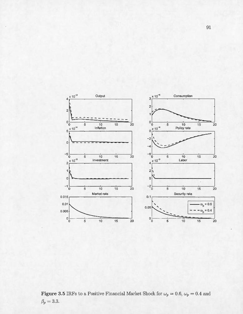
91

:(~----:~~~---- - l :E:=l 0 5 10 15 20 0 5 10 15 20 x 10-4 Inflation x 10-4 Policy rate

_}- ----·-- ~ 1 :~~1 0 5 10 15 20 0 5 10 15 20

-~[ :- - '~•~t~oot •

1

_f' : ~001 : j

0 5 1 0 15 20 0 5 1 0 15 20

Market rate

:::;t;: 0 5 10 15 20

Security rate 0.1

' 0.05 -- rop=0.6

~-- -- -rop =0.4

0 0 5 10 15

Figure 3.5 IRFs to a Posit ive Financial Market Shock for wp = 0.6, wp = 0.4 and

(3p = 3.3.

20

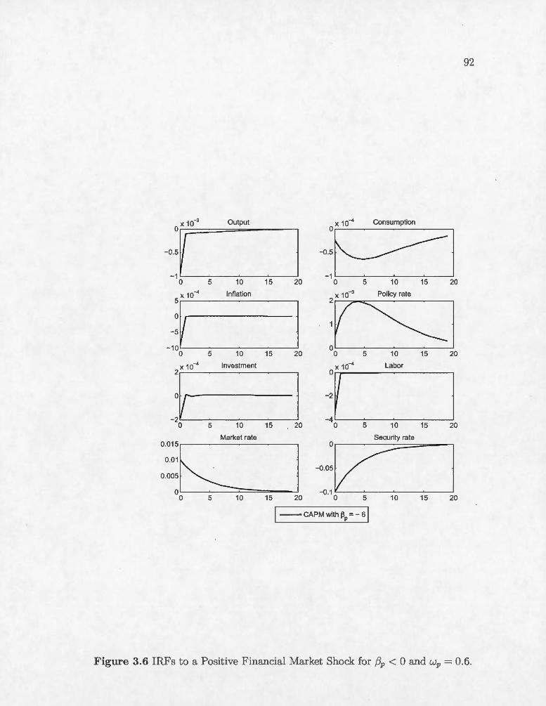
92

' l ~-:~l _,_:r . Output

0 5 10 15 20 0 5 10 15 20

_lo ' • lofl•tioo • l :c:;; l 0 5 1 0 15 20 0 5 1 0 15 20

_{~' ; '"""mool ; l :~110

~ , ' ''.___________.__" ,

0 5 10 15 20 0 5 10 15 20

Market rate Security rate

::;~__,_______,_::&:~1 :o:v= '

0 5 1 0 15 20 0 5 1 0 15 20

1--CAPMwith ~p= - 6 1

Figure 3 .6 IRFs to a Posit ive F inancial Market Shock for {3p < 0 and wp = 0.6.

CONCLUSION

Dans cette thèse, nous analysons les dynamiques à court terme de l'inflation

et les interrelations entre les marchés financiers et l'économie réelle. Le but étant

ici de contribuer à une meilleure application de la politique monétaire. Les deux

premiers chapitres montrent la pertinence de la structure en boucle de production

dans l 'explication de la persistance de l'inflation observée dans les données. Le

troisième chapitre souligne l'importance de la prise en compte des marchés bour­

siers afin de mieux comprendre l'impact des chocs technologique, monétaire et

financiers sur les variables macroéconomiques.

L'objectif du premier chapitre était de dériver une nouvelle courbe de Phillips

néo-keynésienne ( KPC) , à travers un modèle DSGE où nous incorporons les in­

puts intermédiaires et le trend d 'inflation positif. Comme résultat principal, nous

trouvons que les biens intermédiaires semblent avoir un effet plus important sur

la pente de la NKPC que le trend d 'inflation positif.

Cette analyse est approfondie dans le deuxième chapitre où nous simulons

un modèle DSGE en présence toujours des deux: ingrédients, afin de confronter

les autocorrélations de l'inflation du modèle à celles observées dans les données

américaines. Nous trouvons ici que les biens intermédiaires donnent une meilleure

explication de l évidence empirique sur la persistance de l'inflation que ne le fait

le trend d 'inflation positif, confortant ainsi les conclusions du premier chapitre.

Enfin, la contribution du dernier chapitre est une modélisation explicite d 'un

secteur de marchés financiers , plus particulièrement , le marché boursier dans les

modèles DSGE. Pour ce faire nous tenons compte des décisions des ménages sur

les marchés financiers grâce au modèle d 'évaluation des actifs financiers (CAPM)

de Fama et French (2004). Puis, les dynamiques du marché boursier sont décrites

en s'appuyant sur le mouvement brownien géométrique. Ainsi, nous montrons

94

que nos connaissances standard des effets des chocs technologique et de politique

monétaire sur les variables macroéconomiques semblent être modifiées dans ce

nouveau cadre d 'analyse. Nous suggérons aussi qu'un choc au marché financier

a des conséquences non négligeables sur le taux d 'intérêt nominal qui est par

ailleurs l'instrument de politique monétaire. En outre, notre cadre d analyse

reproduit mieux certaines caractéristiques clés du l'économie U.S. , en l'occurrence,

les volatilités et autocorrélations des principales variables macroéconomiques ainsi

que leurs corrélations avec l'output.

APPENDIX A

FINANCIAL MARKETS AND THE CAPITAL ASSET PRICING MODEL IN A DSGE FRAMEWORK

Data sourced from St. Louis Fed, and Kenneth French 's data library on the

official Tuck at Dartmouth MBA school home page.

1. Stock market priees are measured by Standard and Poor 500 Index

(SP500).

2. The stock market volatility is mea.CJmed by the Volatility of Stock Priee

Index for United States (DDS 101USA066NWDB).

3. Stock market retmn rates are measured using Fama/French Benchmark

Factors, CRSP Quarterly data.

4. Financial Accounts of the United States; Federal Reserve Statistical

Release. Z.1 Statistical Release for Dec 11 , 2014; 1.205 (Q), 1 .209 (Q) ,

1.213 (Q).

-------- - ---- - --- - -

BIBLIOGRAPHY

[1] Aruoba, S.B ., Cuba-Borda, P. , Schortheide, F. , 2013. "Macroeconomie Dy­

namics Near the ZLB: A Tale of Two Equilibria." PIER, Working Paper,

14-035.

[2] Ascari, G ., 2004. "Staggered Priees and Trend Inflation: Some Nuisances."

Review of Economie Dynamics, 7, 642-67.

[3] Ascari , G. , Ropele, T ., 2007. "Optimal Monetary Policy Under Low Trend

Inflation." Jo~1,rnal of Monetary Economies, 54, 2568-2583.

[4] Barmish , B.R. , Primbs, J .A., 2011. "On Arbitrage Possibilities Via Linear

Feedback in an Idealized Brownian Motion Stock Market." Proceedings of

the IEEE Conference on Decision and Control, Orlando.

[5] Barthélemy, J. , Marx, M., 2013. "A Discrete Monetary Policy Framework.

An Application to the Japanese Economy." vVorking Paper.

[6] Basu, S. , 1995. ' Intermediate Goods and Business Cycles: Implications for

Productivity and \iVelfare." American Economie Review, 85(3), 512-531.

[7] Basu, S. , Fernald, J .G., 1997. "Aggregate Productivity and Aggregate Tech­

nology." International Finance Discussion Papers.

[8] Basu, S. , Fernald, J .G. , 2000. "Why Is Productivity Procyclical? Why Do

We Care? " NBER (Cambridge, MA), Working Paper No. 7040.

[9] Basu, S. , Kimball, M.S. , 1997. "Cyclical Productivity \vith Unobserved Input

Variation. " NBER (Cambridge, MA) , (Cambridge, MA) \iVorking Paper No.

5915.

[10] Basu, S. , Taylor , A.M. , 1999a. "Business Cycles in International Historical

Perspective." NBER (Cambridge, MA) , (Cambridge, 1tiA) \iVorking Paper

No. 7090.

-- - - ---- ---------------------

97

[11] Basu, S., Taylor, A.M., 1999b. "Business Cycles in International Historical

Perspective." Journal of Economie Perspectives, 13(2) , 45-68.

[12] Bergin , P., Feenstra, R.C., 2000. "Staggered Priee Setting and Endogenous

Persistence.' Journal of Monetary Economies, 45, 657-680.

[13] Bils, M. , Klenow, P.J. , 2004. "Sorne Evidence on the Importance of Sticky

Priees." Jo?trnal of Political Economy, 112(5) , 947-985.

[14] Black, F ., Scholes, M., 1973. "The Pricing of Options and Corporate Liabil­

ities." The Journal of Political Economy, 81(3) , 637-654.

[15] Bodie, Z., Kane, A., Marcus, A.J. , Perrakis, S., Ryan, P.J. , 2005. "Invest­

ments. " Fifth Canadian Edition, McGraw-Hill Ryerson.

[16] Boldrin, Z. , Christiano, A., Fisher, A.J., 2001. "Habit Persistence, Asset

Returns, and the Business Cycle." The American Economie Review, 91(1) ,

149-166.

[17] Bouakez, H. , Cardia, E. , Ruge-Murcia, F.J. , 2005. "Habit Formation and

the Persistence of Monetary Shocks." Journal of Monetary Economies, 52,

1073-1088.

[18] Calvo, G.A. , 1983. "Staggered Priees in a Utility-Maximizing Framework.''

Journal of Monetary Economies, 12, 383-398.

[19] Chari, V.V. , Kehoe, P.J. , McGrattan, E.R., 2000. "Sticky Priee :tvlodels of the

Business Cycle: Can the Contract Multiplier Solve the Persistence Problem?

" Journal of The Econometrie Society: Econometrica, 68(5), 1151-1179.

[20] Chari, V.V., Kehoe, P.J. , McGrattan, E.R. , 2009. "New Keynesian 1/Iodels:

Not Yet Useful for Policy Analysis. " American Economie Journal: Macroe­

conomies, 1(1), 242-66.

[21] Christensen, I. , Dib, A. , 2008. "The financial accelerator in an estimated New

Keynesian model." Review of Economie Dynamics, 11, 155-178.

[22] Christiano , L.J ., Eichenbaum, M. Evans, C.L. , 2005. "Nominal Rigidities

and the Dynamic Effects of a Shock to Monetary Policy." Journal of Political

Economy, 113(1), 1-45.

98

[23] Cogley, T. , Sbordone, A.M. , 2005. "A Search for a St ructural Phillips Curve.

" Federal Reserve Bank of N ew York Staff Reports, No. 203.

[24] Cogley, T. , Sbordone, A.M. , 2008. "Trend Inflation, Indexation, and Infla­

tion Persistence in the ew Keynesian Phillips Curve" Am erican Economie

Review, 98(5) , 2101-2126.

[25] Coibion 0. , Gorodnichenko , Y., 2011 . "Monetary Policy, Trend Inflation,

and the Great Moderation: An Alternative Interpret ation. " American Eco­

nomie Review, 101(1) , 341-70.

[26] Coibion, 0 ., Gorodnichenko, Y. , Wieland, J. , 2012. "The Optimal Inflation

Rate in New Keynesian Models: Should Central Banks Raise Their Inflation

Targets in Light of the Zero Lower Bound?" The Review of Economie Studies,

79, 1371-1406.

[27] Cooley, T .F ., Prescott , E.C. , 1995. "Economie Growt h and Business Cycles."

In, Frontiers of Business Cycle Research, edited by Cooley T.F. , Princeton

University Press.

[28] De Paoli, B. , Scott , A., Weeken, 0. , 2010. "Asset pricing implications of

a New Keynesian model" Journal of Economie Dynamics and Control, 34

2056-2073.

[29] Dib, A. , 2010. "Banks, Credit Market Frictions, and Business Cycles ." B ank

of Canada, vVorking Paper.

[30] Dotsey, M., King, R.G. , 2006. "Production, and Persistence." Journal of the

European Economie Association, 4(5) , 893-928.

[31] Eichenbaum, M. , Fisher , J.D .1tl 2004. "Evaluating the Calvo Model of St icky

Priees." NBER, vVorking Paper o. 10617.

[32] Eichenbaum, M. , Fisher, J .D.M, 2007. "Estimating the Frequency of Priee

Re-Optimization in Calvo-Style Models. " Journal of Monetary Economies,

54(7) , 2032-2047.

[33] El Omari, S., Phaneuf, L. , 2011. "The Mult iplier for Priee St ickiness." vVork­

ing Paper , Université du Québec à Montréal .

[34] Erceg, C.J ., Levin, A.T ., 2003. "Imperfect credibility and inflation persis­

tence." Journal of Monetary Economies, 50 , 915-944.

99

[35] Ermogenous, A., 2005. 'Brownian Motion and its Applications in the Stock

Market." Working Paper.

[36] Falagiarda M., 2013. "Evaluating Quant itative Easing: A DSGE Approach."

\iVorking Paper , University of Balogna.

[37] Fama E.F., 1996. "Multifactor Portfolio Efficiency and Multifactor Asset

Pricing." Journal of Financial and Quantitative Analysis, 31(4) , 441-465.

[38] Fama, E .F. , French, KR. , 2004. "The Capital Asset Pricing Madel: Them·y

and Evidence." Journal of E conomie Perspectives, 18(3) , 25-46.

[39] Fama, E.F. , French, K.R. , 1996. "l\!Iultifactor Explanations of Asset Pricing

Anomalies.' The Journal of Finance, 51(1), 55-84.

[40] Fama, E .F. , French, KR. , 1993. "Common risk factors in the returns on

stocks and bonds." Journal of Financial Economies, 33, 3-56.

[41] Fornero, J ., 2011. "Introducing Financial Assets into Structural Models."

Central Bank of Chile, Working Papers No 625.

[42] Fuhrer, J. , 2000. "Optimal monetary Policy in a Madel with Habit Forma­

tion. " American Economie Review, 90(3) , 367-390.

[43] Gagnon, E., Khan, H., 2005 . " w Phillips Curve under Alternative Pro­

duction Technologies for Canada, the United States, and the Euro Area."

European Economie Review, 49, 1571-1602.

[44] Gall, J. , Gertler , M. , 1999. "Inflation Dynamics: a Structural Econometrie

Analysis ." Journal of Moneta'T"'IJ Economies, 44, 195-222.

[45] Gavin W ., Keen, B. , Richter , A. Throckmorton, N. , 2013 . "Global Dynamics

at the Zero Lower Bound. ' A UWP 17.

[46] Groth, C., 2005. "Estimat ing UK capital adjustment costs." Bank of England

Working Paper, no. 258.

[47] Groth, C., 2006. "Calibrating capital adjustment costs in the New-Keynesian

madel. " Economies Letters, 93 , 26-30.

[48] Ranes C. , 1996. "Changes in the Cyclical Behavior of Real Wage Rates, 1870-

1990." Journal of Economie History, Cambridge University Press 56(04) ,

837-861.

100

[49] Ranes, C., 1999. "Degrees of Processing and Changes in the Cyclical Behavior

of Priees in the United States, 1869-1990." Journal of Money, Credit, and

Banking, 31(1), 35-53.

[50] Huang, K.X.D. , Liu, Z., 2001. "Production Chains and General Equilibrium

Aggregate Dynamics." Journal of Monetary Economies, 48, 437-462.

[5 1] Huang K.X.D. , Liu, Z. , Phaneuf, L. , 2004. "\Vhy Does the Cyclical Behavior

of Real vVages Change over Time." American Econom.ic Review, 94(4) , 836-

856.

[52] Ireland, P.N. , 2007. "Changes in the Federal Reseve's Inflation Target:

Causes and Consequences." Journal of Money, Credit and Banking, 39(8) ,

1851-82.

[53] Jorgensen, D.W. , Gollop, F.M., Fraumeni, B.M., 1987. "Productivity and

U.S. Economie Growth." Cambridge MA, Harvard University Press.

[54] Justiniano , J. , Primiceri G.E. , 2008. "The Time-Varying Volatility of

Macroeconomie Fluctuations." American Economie Review, 98(3) , 604-641.

[55] Justiniano, A. , Primicieri , G.E. , Tambalotti, A. , 2011. "Investment Shocks

and the Relative Priee of Investment. " Review of Economie Dynamics, 14(1) ,

101-121.

[56] Kendall, M.G., Hill , A.B., 1953. "The Analysis of Economie Time-Series­

Part-I: Priees." Journal of the Royal Statistical Society, Series A (General) ,

116(1), 11-34.

[57] Khan, H. , Tsoukalas, J ., 2012. ' The Quantitative Importance of News Shocks

in Estimated DSGE models." Vlorking Paper.

[58] King R. , Rebelo , S. 2000. "Resuscitating Real Business Cycles.' NBER,

\i\lorking Paper No. 7534.

[59] King, R.G. , Watson, M.W. , 1996. "Iv1oney, Priees, Interest Rates and the

Business Cycle." Review of Economies and Statistics, 78, 35-53.

[60] Lintner , J. , 1965. "The Valuation of Risk Assets and the Selection of Risky

Investments in Stock Portfolios and Capital Budgets." Review of Economies

and Statistics, 47(1), 13-37.

101

[61] Liu, Z. , Phaneuf, L. , 2007. "Technology Shocks and Labor Market Dynamics:

Sorne Evidence and Theory." Journal of Monetary Economies, 57, 2534-2553.

[62] Lochowski , R.M. , Thagunna, K.S. , 2013. "Analyzing the Nepali Stock Market

with Stochastic Models." \iVorking paper.

[63] Markowitz, H. , 1959. "Port folio Selection: Efficient Diversification of Invest­

ments." Cowles Foundation Monograph, No. 16. New York: John \iViley &

Sons, Inc.

[64] McCallum, B. , Ielson, E. , 1999. "Nominal Income Targeting in an Open­

Economy Optirnizing Model." Journal of Monetary Economies, 43, 553-578.

[65] Miao, J ., Wang, P. , Xu, Z., 2012. "A Bayesian DSGE Model of Stock Market

Bubbles and Business Cycles." Working paper.

[66] Nakamura, E. , Steinsson, J ., 2008. "Five Facts About Priees : A Reevaluation

of Menu Cost Iodels." Quaterly Journal of Economies, 123(4), 1415-1464.

[67] Nakamura, E. , Steinsson, J ., 2010. "Monetary Non- eutrality in a Mult i­

Section Menu Cost Models ." Quaterly Journal of Economies, 125(3) , 961-

1013.

[68] Nelson, E. , 1998. "Sluggish Inflation and Optimizing Models of the Business

Cycle." Journal of Monetary Economies, 42, 303-322.

[69] Osborne, M.F.M., 1959. "Brownian Motion in the Stock Market." Operations

Research, 7(2) , 145-173.

[70] Phaneuf, L. , Tchakondo , Y. , 2012 . "The New Keynesian Phillips Curve: In­

termediate Goods Meet Positive Trend Inflation." Working Paper, Université

du Québec à Montréal and CIRPÉE.

[71] Pi vetta, F., Reis, R. , 2007. "The persistence of inflation in the United States."

Journal of Economie Dynamics and Controls, 31, 1326-1358.

[72] Ravn, M.O. , Schmitt-Grohoé, S. , Uribe, M. , Uuskula 2008. "Deep Habits

and the Dynamic Effects of Monetary Policy." EU! Working Paper, ECO

2008/40.

[73] Richter, A., Throckmorton, N., 2013. "The Zero Lower Bound: Frequency,

Dura.tion, and Determina.cy." A UWP, 16.

102

[74] Roberts, H.V., 1959. "Stock-Market "Patterns " and Financial Analysis:

Methodological Suggestions." Journal of Finance, 14(1) , 1-10.

[75] Rotemberg, J.J. , Vloodford, M. 1997. ''An Optimization-Based Econometrie

Framework for the Evaluation of Monetary Policy." In: Rotemberg, J.J. ,

Bernanke, B.S . (Eds.) , NBER Macroeconomies Annual 1991. MIT Press,

Cambridge, MA, pp. 297-346.

[76] Samuelson, P.A., 1965. "Rational Theory of Warrant Pricing. " Industrial

Management R eview, (6)2, 13-39.

[77] Sbordone, A.M. , 2007. "Inflation persistence: Alternative interpretations and

policy ünplications." Journal of Monetary Economies, 54, 1311-1339.

[78] Shapiro, M.D., 1986. "The Dynamic Demand for Capital and Labor. " NBER

(Cambridge, MA) , vVorking Paper o. 1899.

[79] Sharpe, \V.F. , 1964. "Capital Asset Priees: A Theory of Market Equilibrium

under Conditions of Risk." Journal of Finance, (19)3, 425-442.

[80] Smets, F. , \Vouters, R. 2007. "Shocks and Frictions in U.S. Business Cycles:

a Bayesian DSGE Approach. " American Economie R e1;iew, 97, 586-606.

[81] Smets, F ., Wouters , R. , 2003. "An Estimated Dynamic Stochastic General

Equilibrium Model of the Euro Area." Journal of the European E conomie

Association, 1(5) , 1123-1175.

[82] Smets, F. , Vvouters , R. , 2007. "Shocks and Frictions in U.S. Business Cycles:

a Bayesian DSGE Approach." American Economie Review, 97, 586-606.

[83] Taylor, J .B., 1999. "Staggered Priees and Wage Setting in Macroeconomies.

" In Handbook of Macroeconomies, vol. lB , edited by Taylor , J.B., Woodford,

M. Amsterdam: Elsevier Sei.

[84] \Vest , K.D. , 2007. "Comment on Argia M. Sbordone" "Inflation Persistence:

Alternative Interpretations and Policy Implications." Journal of MonetaTy

Economies, 1340-1343.

[85] \Voodford, M. , 2003. "Interest and Priees. Foundations of a The01·y of Mon­

etary Policy." Princeton University PTess, Princeton , NJ.

103

[86] \iVoodford , M., 2005. "Firm-Specific Capital and the New Keynesian Phillips

Curve.)) International Journal of Central Banking, 1(2) , 1-46.

[87] Vo/oodford , M. , 2007. ' Interpreting Inflation Persistence: Comments on the

Conference on Quantitative Evidence on Priee Determination .)) Journal of

Money, Credit and Banking, 39(sl), 203-210.