Equity Valuation Using Multiples

Jing Liu

Anderson Graduate School of Management

University of California at Los Angeles

(310) 206-5861

jing.liu@anderson.ucla.edu

Doron Nissim

Columbia University

Graduate School of Business

(212) 854-4249

dn75@columbia .edu

and

Jacob Thomas

Columbia University

Graduate School of Business

(212) 854-3492

jkt1@columbia.edu

March, 2001

We received helpful comments from David Aboody, Sanjay Bhagat, Ted Christensen, Glen Hansen, Jack

Hughes, Jim Ohlson, Stephen Penman, Phil Shane, Michael Williams, and seminar participants at the

AAA Annual Meeting at Philadelphia, University of Colorado, Columbia University, Copenhagen

Business School, Ohio State University, and UCLA.

Equity Valuation Using Multiples

Abstract We examine the valuation performance of a comprehensive list of value drivers and find that multiples

derived from forward earnings explain stock prices remarkably well for most firms: pricing errors are

within 15 percent of stock prices for about half of our sample. In terms of relative performance, the

following general rankings are observed consistently each year: forward earnings measures are followed

by historical earnings measures, cash flow measures and book value of equity are tied for third, and sales

performs the worst. Contrary to the popular view that different industries have different “best” multiples,

we find that these overall rankings are observed consistently for almost all industries examined. Adjusting

the ratio formulation typically followed in practice to allow for an intercept offers some improvement,

especially for multiples that perform poorly. No improvement is observed, however, when we consider

more complex measures of intrinsic value based on short-cut residual income models (where forward

earnings are combined with book values, estimated discount rates, and generic terminal value estimates).

Since we require analysts’ earnings and growth forecasts and positive values for all measures, our results

may not be representative of the many firm-years excluded from our sample.

1

Equity Valuation Using Multiples

1. Introduction

In this study we examine the proximity to stock prices of valuations generated by multiplying a

value driver (such as earnings) by the corresponding multiple, where the mult iple is obtained from the

ratio of stock price to that value driver for a group of comparable firms. While multiples are used

extensively in practice, there is little published research in the academic literature documenting the

absolute and relative performance of different multiples.1 We seek to investigate the performance of a

comprehensive list of multiples, and also examine a variety of related issues, such as the variation in

performance across industries and over time and the performance improvement obtained by using

alternative approaches to compute multiples.

Although the actual valuation process used by market participants is unobservable, we assume

that stock prices can be replicated by comprehensive valuations that convert all available information into

detailed projections of future flows. Given this efficient markets framework for traded stocks, what role

do multiples play? Even in situations where market valuations are absent, either because the equity is

privately-held or because the proposed publicly traded entity has not yet been created (e.g., mergers and

spinoffs), is there a role for multiples vis-à-vis comprehensive valuations? While the multiple approach

bypasses explicit projections and present value calculations, it relies on the same principles underlying the

more comprehensive approach: value is an increasing function of future payoffs and a decreasing function

of risk. Therefore, multiples are used often as a substitute for comprehensive valuations, because they

1 Studies offering descriptive evidence include Boatsman and Baskin [1981], LeClair [1990], and

Alford [1992]. Recently, a number of studies have examined the role of multiples for firm valuation in specific contexts, such as tax and bankruptcy court cases and initial public offerings (e.g., Beatty, Riffe, and Thompson [1999], Gilson, Hutchkiss and Ruback [2000], Kim and Ritter [1999], and Tasker [1998]).

2

communicate efficiently the essence of those valuations. Multiples are also used to complement

comprehensive valuations, typically to calibrate those valuations and to obtain terminal values.2

In effect, our study documents the extent to which different value drivers serve as a summary

statistic for the stream of expected payoffs, and comparable firms resemble the target firm along

important value attributes, such as growth and risk. We first evaluate value drivers using the conventional

ratio representation (i.e., price doubles when the value driver doubles). To identify the importance of

incorporating the average effect of omitted variables, we extend the ratio representation to allow for an

intercept in the price/value driver relation. To study the impact of selecting comparable firms from the

same industry, we contrast our results obtained by using industry comparables (the middle category from

the Sector/Industry/Group classification provided by IBES) with results obtained when all firms available

each year are used as comparables. As in prior research, we evaluate performance by examining the

distribution of percent pricing errors (actual price less predicted price, scaled by actual price).

The value drivers we consider include measures of historical cash flow, such as cash flow from

operations and EBITDA (earnings before interest, taxes, depreciation, and amortization), and historical

accrual-based measures, such as sales, earnings, and book value of equity. We also consider forward-

looking measures derived from analysts’ forecasts of EPS (earnings per share) and long-term growth in

EPS, such as 2-year out consensus EPS forecasts and PEG (price-earnings-growth) ratios (e.g., Bradshaw

[1999a; 1999b]). Since sales and EBITDA should properly be associated with enterprise value (debt plus

equity), rather than equity alone, for those two value drivers we also consider multiples based on

enterprise value (market value of equity plus book value of debt). Finally, we consider short-cut intrinsic

value measures based on the residual income model that have been used recently in the academic

literature (e.g., Frankel and Lee [1998], and Gebhardt, Lee, and Swaminathan [2001]).

2 Another very different role for multiples that has been examined in the literature is the identification

of mispriced stocks. We do not investigate that role because we assume market efficiency. Two such market inefficiency studies are Basu [1977] and Stattman [1980]), where portfolios derived from earnings and book value multiples are shown to earn abnormal returns.

3

The following is an overview of the relative performance of different value drivers: (1) forward

earnings perform the best, and performance improves if the forecast horizon lengthens (1-year to 2-year to

3-year out EPS forecasts) and if earnings forecasted over different horizons are aggregated; (2) the

intrinsic value measures, based on short-cut residual income models, perform considerably worse than

forward earnings 3; (3) among drivers derived from historical data, sales performs the worst, earnings

performs better than book value; and IBES earnings (which excludes many one-time items) outperforms

COMPUSTAT earnings; (4) cash flow measures, defined in various forms, perform poorly; and (5) using

enterprise value, rather than equity value, for sales and EBITDA further reduces performance.

Turning from relative performance to absolute performance, forward earnings measures describe

actual stock prices reasonably well for a majority of firms. For example, for 2-year out forecasted

earnings, approximately half the firms have absolute pricing errors less than 16 percent. The dispersion of

pricing errors increases substantially for multiples based on historical drivers, such as earnings and cash

flows, and is especially large for sales multiples.

Some other important findings are as follows: (1) performance improves when multiples are

computed using the harmonic mean, rela tive to the mean or median ratio of price to value driver for

comparable firms, (2) performance declines substantially when all firms in the cross-section each year are

used as comparable firms, (3) allowing for an intercept improves performance mainly for poorly-

performing multiples, (4) relative performance is relatively unchanged over time and across industries.

Our findings have a number of implications for valuation research. First, we confirm the validity

of two precepts underlying the valuation role of accounting numbers: (1) accruals improve the valuation

properties of cash flows, and (2) despite the importance of top-line revenues, its value relevance is limited

until it is matched with expenses. Second, we confirm that forward earnings contain considerably more

value-relevant information than historical data, and they should be used as long as earnings forecasts are

3 Bradshaw [1999a and 1999b] observes results that are related to ours. He finds that valuations based

on PEG ratios explain more variation in analysts’ target prices and recommendations than more complex intrinsic value models.

4

available. Third, contrary to general perception, different industries are not associated with different “best

multiples.” Finally, our investigation of the signal/noise tradeoff associated with the more complex

intrinsic value drivers based on the residual income model suggests that even though these measures

utilize more information than that contained in forward earnings and impose a structure derived from

valuation theory on that information, measurement error associated with the additional variables required,

especially terminal value estimates, negatively impacts performance.4

These findings are associated with certain caveats. Since we exclude firms not covered by IBES,

typically firms with low and medium market capitalization, we are uncertain about the extent to which

our results extend to those firms. Even firms with IBES data are not fully represented in our sample, since

we exclude firm-years with negative values for any value driver. In particular, our results may not be

descriptive of start-up firms reporting losses and high growth firms with negative operating cash flows.

2. Prior Research

While textbooks on valuation (e.g., Copeland, Koller, and Murrin [1994], Damodaran [1996] and

Palepu, Healy, and Bernard [2000]) devote considerable space to discussing multiples, most published

papers that study multiples examine a limited set of firm-years and consider only a subset of multiples,

such as earnings and EBITDA. Also, comparisons across different studies are hindered by methodological

differences.

Among commonly used value drivers, historical earnings and cash flows have received most of

the attention. Boatsman and Baskin [1981] compare the valuation accuracy of P/E multiples based on two

sets of comparable firms from the same industry. They find that valuation errors are smaller when

comparable firms are chosen based on similar historical earnings growth, relative to when they are chosen

randomly. Alford [1992] investigates the effects of choosing comparables based on industry, size (risk),

and earnings growth on the precision of valuation using P/E multiples. He finds that pricing errors decline

4 Given our efficient markets framework, we do not investigate here whether the relatively poor

performance of the intrinsic value measures is due to an inefficient market that values stocks using

5

when the industry definition used to select comparable firms is narrowed from a broad, single digit SIC

code to classifications based on two and three digits, but there is no additional improvement when the

four-digit classification is considered. He also finds that controlling for size and earnings growth, over

and above industry controls, does not reduce valuation errors.

Kaplan and Ruback [1995] examine the valuation properties of the discounted cash flow (DCF)

approach for highly leveraged transactions. While they conclude that DCF valuations approximate

transacted values reasonably well, they find that simple EBITDA multiples result in similar valuation

accuracy. Beatty, Riffe, and Thompson [1999] examine different linear combinations of value drivers

derived from earnings, book value, dividends, and total assets. They derive and document the benefits of

using the harmonic mean, and introduce the price-scaled regressions we use. They find the best

performance is achieved by using (1) weights derived from harmonic mean book and earnings multiples

and (2) coefficients from price-scaled regressions on earnings and book value.

In a recent study, Baker and Ruback [1999] examine econometric problems associated with

different ways of computing industry multiples, and compare the relative performance of multiples based

on EBITDA, EBIT (or earnings before interest and taxes), and sales. They provide theoretical and

empirical evidence that absolute valuation errors are proportional to value. They also show that industry

multiples estimated using the harmonic mean are close to minimum-variance estimates based on Monte

Carlo simulations. Using the minimum-variance estimator as a benchmark, they find that the harmonic

mean dominates alternative simple estimators such as the simple mean, median, and value-weighted

mean. Finally, they use the harmonic mean estimator to calculate multiples based on EBITDA, EBIT, and

sales, and find that industry-adjusted EBITDA performs better than EBIT and sales.

Instead of focusing only on historical accounting numbers, Kim and Ritter [1999], in their

investigation of how initial public offering prices are set using multiples, add forecasted earnings to a

conventional list of value drivers, which includes book value, earnings, cash flows, and sales. Consistent

multiples of forward earnings. We find evidence inconsistent with that explanation in a separate paper (Liu, Nissim, and Thomas [2001]).

6

with our results, they find that forward P/E multiples (based on forecasted earnings) dominate all other

multiples in valuation accuracy, and that the EPS forecast for next year dominates the current year EPS

forecast.

Using large data sets could diminish the performance of multiples, since the researcher selects

comparable firms in a mechanical way. In contrast, market participants may select comparable firms more

carefully and take into account situation-specific factors not considered by researchers. Tasker [1998]

examines across-industry patterns in the selection of comparable firms by investment bankers and

analysts in acquisition transactions. She finds the systematic use of industry-specific multiples, which is

consistent with different multiples being more appropriate in different industries.5

3. Methodology

In this section we describe the different value drivers considered, and the methodology used in

the two stages of our analyses: estimating the price/value driver relation without and with an intercept.

3.1 Value Drivers

The following is a list of value drivers examined in this paper. We have grouped them based on

whether they refer to cash flows or accruals, whether they relate to stocks or flows, and whether they are

based on historical or forward-looking information. 6 We provide a brief description here for some

variables that readers may not be familiar with (details for all variables are provided in Appendix A) and

then describe the links drawn in the prior literature between different value drivers and equity value. (1)

Accrual flows: sales, actual earnings from COMPUSTAT (CACT) and actual earnings from IBES

(IACT). (2) Accrual stocks: book value of equity (BV). (3) Cash flows: cash flow from operations (CFO),

free cash flow to debt and equity holders (FCF), maintenance cash flow (MCF), equal to free cash flows

for the case when capital expenditures equal depreciation expense, and earnings before interest, taxes,

5 Since it is not clear whether the objective of investment bankers/analysts is to achieve the most

accurate valuation in terms of smallest dispersion in percent pricing errors, our results may not be directly comparable with those in Tasker [1998].

6 Some value drivers are not easily classified. For example, Sales, which is categorized as an accrual flow, could contain fewer accruals than EBITDA, which is categorized as a cash flow measure.

7

depreciation and amortization (EBITDA). (4) Forward looking information: consensus (mean) one year

and two year out earnings forecasts (EPS1, and EPS2), and two forecasted earnings-growth combinations

(EG1=EPS2*(1+g) and EG2=EPS2*g) which are derived from EPS2 and g (the mean long-term EPS

growth forecast provided by analysts). (5) Intrinsic value measures (P1*, P2*, and P3*): These measures

are based on the residual income (or abnormal earnings) valuation approach, where equity value equals

the book value today plus the present value of future abnormal earnings. Abnormal earnings for years +1

to +5, projected from explicit or implied earnings forecasts for those years, are the same for the first two

measures. After year +5, abnormal earnings are assumed to remain constant for P1* and equal zero for

P2*. For P3*, the level of profitability (measured by ROE) is assumed to trend linearly from the level

implied by earnings forecasted for year +3 to the industry median by year +12, and abnormal earnings are

assumed to remain constant thereafter. (6) Sum of forward earnings (ES1 and ES2): These measures

aggregate the separate forward earnings forecasts. ES1 is the sum of the EPS forecasts for years +1 to +5,

and ES2 is the sum of the present value of those forecasts. 7 As explained later, these two measures are

designed to provide evidence on the poor performance of the intrinsic value measures.

Value drivers based on accruals, which distinguish accounting numbers from their cash flow

counterparts, have been used extensively in multiple valuations. Book value and earnings, which are often

assumed to represent “fundamentals,” have been linked formally to firm value (e.g,, Ohlson [1995] and

Feltham and Ohlson [1995]). Although the use of sales as a value driver has less theoretical basis, relative

to earnings and cash flows, we consider it because of its wide use in certain emerging industries where

earnings and cash flow are perceived to be uninformative.

At an intuitive level, accounting earnings could be more value-relevant than reported cash flows

because some cash flows do not reflect value creation (e.g., asset purchases/sales), and accruals allow

managers to reflect their judgment about future prospects. The COMPUSTAT EPS measure we consider

is reported primary EPS excluding extraordinary items and discontinued operation and the IBES EPS

7 We thank Jim Ohlson for suggesting ES1.

8

measure is derived from reported EPS by deleting some one-time items, such as write-offs and

restructuring charges. To the extent that the IBES measure is a better proxy for “permanent” or “core”

earnings expected to persist in the future, it should exhibit superior performance.

The use of cash flow multiples in practice appears to be motivated by the implicit assumption that

reported cash flow is the best available proxy for the future cash flows that underlie stock prices, and by

the feeling that they are less susceptible to manipulation by management. The four cash flow measures we

consider remove the impact of accruals to different extents. EBITDA adjusts pre-tax earnings to debt and

equity holders for the effects of depreciation and amortization only. CFO deducts interest and taxes from

EBITDA and also deducts the net investment in working capital. FCF deducts from CFO net investments

in all long-term assets, whereas MCF only deducts from CFO an investment equal to the depreciation

expense for that year.

The potential for analysts’ EPS forecasts to reflect value-relevant data not captured by historical

earnings has long been recognized in the literature. For example, Liu and Thomas [2000] find that

revisions in analysts’ earnings forecasts along with changes in interest rates explain a substantially larger

portion of contemporaneous stock returns than do earnings surprises based on reported earnings.

Consensus estimates are often available for forecasted earnings for the current year (EPS1) and the

following year (EPS2). Consensus estimates are also frequently available for the long-term growth

forecast (g) for earnings over the next business cycle (commonly interpreted to represent the next 5

years). The measure EG1 (=EPS2*(1+g)), which is an estimate of three-year out earnings, should reflect

value better than EPS2, if three-year out earnings reflect long-term profitability better than two-year out

earnings.

While the second earnings-growth measure EG2 (=EPS2*g) also combines the information

contained in EPS2 and g, it imposes a different structure. Recently, analysts have justified valuations

using the following rule of thumb: forward P/E ratios (current price divided by EPS2) should equal g. If,

for example, EPS is expected to grow at 30 percent over the next business cycle, then forward P/E should

equal 30. Stated differently, the ratio of forward P/E to g (referred to as the PEG ratio) should equal 1. For

9

certain sectors, such as technology, analysts have suggested that even higher PEG ratios are appropriate.

Using EG2 as a value driver is equivalent to using a PEG ratio obtained from the PEG ratios of

comparable firms.

Several recent studies provide evidence that the intrinsic values derived using the residual income

model explain stock prices (e.g., Abarbanell and Bernard [2000], Claus and Thomas [2000]) and returns

(e.g., Liu and Thomas [2000], Liu [1999]). The three generic patterns we use to project abnormal earnings

past a horizon date have been considered in Frankel and Lee [1998] (P1*), Palepu, Healy, and Bernard

[2000] (P2*), and Gebhardt, Lee, and Swaminathan [2001] (P3*). Although these generic approaches do

not allow for firm-specific growth patterns for abnormal earnings past a terminal date, they offer a

convenient alternative to comprehensive valuations as long as observed long-term growth patterns tend to

converge to the generic patterns assumed by these measures.

While the two final earnings sum measures we consider (ES1 and ES2) have not been discussed

in the literature, we examine them to understand better the poor performance observed for the intrinsic

value measures. ES1 simply sums the earnings forecasted for years +1 to +5, and ES2 attempts to control

heuristically for the timing and risk of the different earnings numbers by discounting those forecasted

earnings before summing them. If both ES1 and ES2 perform poorly, relative to simple forward earnings

multiple (e.g., EPS2) the earnings projected for years +3 to +5 probably contain considerable error. If ES1

performs well, but ES2 does not, estimation errors in the firm-specific discount rates used to discount

flows at different horizons are responsible for the poor performance of the intrinsic value measures. If

both ES1 and ES2 perform well, the poor performance of intrinsic value measures is probably because the

assumed terminal values in each case diverge substantially from the market’s estimates of terminal

values.

We also consider the impact of using enterprise value (TP), rather than equity value, for sales and

EBITDA multiples, since both value drivers reflect an investment base that includes debt and equity. We

measure TP as the market value of equity plus the book value of debt. To obtain predicted share prices,

10

we estimate the relation between TP and the value driver for comparable firms, generate predicted TP for

target firms, and then subtract the book value of their debt.

3.2 Traditional Multiple Valuation

In the first stage of our analysis, we follow the traditional ratio representation and require that the

price of firm i (from the comparable group) in year t (pit) is directly proportional to the value driver:

itittit xp εβ += (1)

where itx is the value driver for firm i in year t, tβ is the multiple on the value driver and tε is the

pricing error. To improve efficiency, we divide equation (1) by price:

it

it

it

itt pp

x εβ +=1 . (2)

Baker and Ruback [1999] and Beatty, Riffe, and Thompson [1999] demonstrate that estimating the slope

using equation (2) rather than equation (1) is likely to produce more precise estimates because the

valuation error (the residual in equation (1)) is approximately proportional to price.

When estimating βt, we elected to impose the restriction that expected percent pricing errors

(E[ε/p]) be zero, even though an unrestricted estimate for βt from equation (2) offers a lower value of

mean squared percent pricing error. Empirically, we find that our approach generates lower pricing errors

for most firms, relative to an unrestricted estimate, but it generates substantially higher errors in the tails

of the distribution. 8 By restricting ourselves to unbiased percent pricing errors, we are in effect assigning

lower weight to extreme pricing errors, relative to the unrestricted approach. We are also maintaining

consistency with the tradition in econometrics that strongly prefers unbiasedness over reduced dispersion.

8 We estimated equation (2) for comparable firms from the cross-section without imposing the

unbiasedness restriction. (When using comparable firms from the same industry, the estimated multiples for this unrestricted case generated substantial pricing errors.) We find that the percent pricing error distributions for all multiples are shifted to the right substantially, relative to the distributions for the restricted case reported in the paper (our distributions tend to peak around zero pricing error). This shift to the right indicates that the multiples and predicted valuations for the unrestricted case are on average lower than ours. We find that the bias created by this shift causes greater pricing errors for the bulk of the firms not in the tails of the distribution, relative to our restricted case.

11

βt is the only parameter to be estimated in equation (2), and it is determined by the restriction we

impose that percent pricing errors be zero on average, i.e., 0=

it

it

pE

ε. Rearranging terms in equation

(2) and applying the expected value operator, we obtain the harmonic mean of /it itp x as an estimate for

βt:

01 =

−=

it

it

it

it

p

xE

pE

βε

=⇒

it

it

p

xE

1tβ (3)

We multiply this harmonic mean estimate for βt by the target firm’s value driver to obtain a

prediction for the target firm’s equity value, and calculate the percent pricing error as follows:9

it

ittit

it

it

p

xp

p

^

βε −= . (4)

To evaluate the performance of multiples, we examine measures of dispersion, such as the interquartile

range, for the pooled distribution of itit p/ε .

3.3 Intercept Adjusted Multiples

For the second stage of our analysis, we relax the direct proportionality requirement and allow for

an intercept:

ititttit xp εβα ++= . (5)

Many factors, besides the value driver under investigation, affect price, and the average effect of such

omitted factors is unlikely to be zero.10 Since the intercept in equation (5) captures the average effect of

omitted factors, allowing for an intercept should improve the precision of out of sample predic tions.

As with the simple multiple approach, we divide equation (5) by price to improve estimation

efficiency:

9 While some studies measure pricing error as predicted value minus price (e.g., Alford [1992]) we

measure pricing error as price minus predicted value.

12

it

it

it

itt

itt pp

x

p

εβα ++= 1

1 , (6)

Estimating equation (6) with no restrictions minimizes the square of percent pricing errors, but the

expected value of those errors is non-zero.11 For the reasons mentioned in section 3.2, we again impose

the restriction that percent pricing errors be unbiased.12 That is, we seek to estimate the parameters αt and

βt that minimize the variance of itit p/ε , subject to the restriction that the expected value of itit p/ε is

zero:

)]1

(1var[]/)var[()/( varmin,

it

itt

it

tititttititit p

x

ppxpp βαβαε

βα+−=⋅−−= (7a)

.0E .. =

it

it

pts

ε (7b)

It can be shown that the estimates for αt and βt that satisfy (7a) and (7b) are as follows

−

+

−

=

t

t

tt

t

ttt

t

t

t

t

tt

t

ttt

t

t

p

x

pp

xE

pE

pp

xE

p

x

pE

pE

p

x

ppp

xE

,1

cov1

21

varvar1

1,

1cov

1var

22β (8)

−

=

t

t

tt

t

pE

p

xE

1

1 βα (9)

where the different Et[.], var(.), and cov(.) represent the means, variances, and covariances of those

expressions for the population, and are estimated using the corresponding sample moments for the

10 If the relation between price and the value driver is non-linear, the omitted factors include higher

powers of the value driver. 11 In general, this bias could be removed by allowing for an intercept. That avenue is not available,

however, when the dependent variable is a constant (=1), since the intercept captures all the variation in the dependent variable, thereby making the independent variables redundant.

12 As with equation (2), percent pricing errors from the unrestricted approach for equation (6) are higher for most firms (in the middle of the distribution) but there are fewer firms in the tails of the distribution. (See footnote 8.)

13

comparable group. We compute prediction errors, defined by equation (10), and examine their

distribution to determine performance.

it

itttit

it

it

p

xp

p

^^βαε −−

= . (10)

4. Sample and Data

To construct our sample, we merge data from three sources: accounting numbers from

COMPUSTAT; price, analyst forecasts, and actual earnings per share from IBES; and stock returns from

CRSP. As of April of each year (labeled year t+1), we select firm-years that satisfy the following criteria:

(1) COMPUSTAT data items 4, 5, 12, 13, 25, 27, 58, and 60 are non-missing for the previous fiscal year

(year t); (2) at least 30 monthly returns are available on CRSP from the prior 60 month period; (3) price,

actual EPS, forecasted EPS for years t+1 and t+2, and the long term growth forecast are available in the

IBES summary file; and (4) all price to value-driver ratios for the simple multiples (excluding the three

P* and two ES measures) lie within the 1st and 99th percentiles of the pooled distribution. The resulting

sample, which includes 26,613 observations between 1982 and 1999, is used for the descriptive statistics

reported in Table 1.

For the results reported after Table 1, we impose three additional requirements: (1) share price on

the day IBES publishes summary forecasts in April is greater than or equal to $2; (2) all multiples are

positive; and (3) each industry-year combination has at least five observations. The first condition avoids

large pricing errors in the second stage analysis (where an intercept is allowed) due to firms with low

share prices. The second condition avoids negative predicted prices, and the third condition ensures that

the comparable group is not unreasonably small. Regarding the second condition, we discovered that

many firm-years were eliminated because of negative values for two cash flow measures: free cash flow

and maintenance cash flow. More important, preliminary analysis indicated that both measures exhibited

larger pricing errors than the other measures. As a result, we felt that these two measures were unsuitable

for large sample multiples analyses and dropped them from the remainder of our study. The final sample

has 19,879 firm-years.

14

Our sample represents a small fraction of the NYSE+AMAX+NASDAQ population that it is

drawn from: the fraction included varies between 11 percent earlier in the sample period to 18 percent

later in our sample period. The fraction of market value of the population represented, however, is

considerably larger because the firms deleted for lack of analyst data are on average much smaller than

our sample firms. Also, firm-years excluded because they have negative value drivers are potentially

different from our sample, because they are more likely to be young firms and/or technology firms. For

these reasons, our results may not be descriptive of the general population.

We adjust all per share numbers for stock splits and stock dividends using IBES adjustment

factors. If IBES indicates that the consensus forecast for that firm-year is on a fully diluted basis, we use

IBES dilution factors to convert those numbers to a primary basis. We use a discount rate (k t) equal to the

risk-free rate plus beta times the equity risk premium. The risk-free rate is the 10-year Treasury bond

yield on April 1 of year t+1 and we assume the equity premium is 5 percent. We estimate betas using

monthly stock returns and value-weighted CRSP returns over the 60 month period ending in March of

year t+1, and measure beta as the median beta of all firms in the same beta decile. 13

For a subgroup of firm-years (less than 5 percent), we were able to obtain mean IBES forecasts

for all years in the five-year horizon. For all other firms, with less than complete forecasts available

between years 3 and 5, we generate forecasts by applying the mean long-term growth forecast (g) to the

mean forecast for the prior year in the horizon; i.e., )1(*1 gepseps stst += −++ .

We obtain book values for future years by assuming the “ex-ante clean surplus relation” (ending

book value in each future period equals beginning book value plus forecasted earnings less forecasted

dividends). Since analyst forecasts of future dividends are not available on IBES, we assume that the

current dividend payout ratio will be maintained in the future. We measure the current dividend payout as

the ratio of the indicated annual cash dividends to the earnings forecast for year t+1 (both obtained from

13 We use decile median betas, since firm-specific betas are estimated with considerable error.

15

the IBES summary file).14 To minimize biases that could be induced by extreme dividend payout ratios

(caused by forecast t+1 earnings that are close to zero), we Winsorize payout ratios to lie between 10%

and 50%.15

5. Results

The following is an overview of this section. Descriptive univariate statistics for the different

value drivers and bivariate correlations among them are provided in Section 5.1 The distribution of

pricing errors for the traditional no-intercept relation between price and value drivers is provided in

Section 5.2, and the results obtained when an intercept is included are provided in Section 5.3. In both

subsections, the results are reported separately for two sets of comparable firms with data available that

year: all firms from the same industry and all firms in the cross-section. In either case, our analysis is

always conducted out of sample; i.e., the target firm is removed from the group of comparable firms.

Since the traditional approach involves the no-intercept relation and the selection of comparable firms

from the same industry, much of our discussion focuses on that combination, and most of our ancillary

investigations relate only to this combination.

To conduct the analysis using comparable firms from the same industry, we considered

alternative industry classifications. Because of the evidence that SIC codes frequently misclassify firms

(Kim and Ritter [1999]), we use the industry classification provided by IBES, which is indicated to be

based loosely on SIC codes, but is also subject to detailed adjustments.16 The IBES industry classification

has three levels (in increasing fineness): sector, industry, and group. We use the intermediate (industry)

classification level because visual examination of firms included in the same sector suggested it was too

broad a classification to allow the selection of homogeneous firms, and tabulation of the number of firms

14 Indicated annual dividends are four times the most recent quarter’s declared dividends. We use EPS1

as the deflator because it varies less than current year's earnings and is less likely to be close to zero or negative.

15 The impact of altering the dividend payout assumptions on the results is negligible, because it has a very small impact on future book value and an even smaller impact on the computed abnormal earnings.

16 The IBES classification resembles the industry groupings suggested by Morgan Stanley.

16

in different groups suggested it was too narrow to allow the inclusion of sufficient comparable firms

(given the loss of observations due to our data requirements).

Because of the volume of results generated, we report only some representative results and

describe briefly some interesting extensions. In particular, we do not report on tests of statistical

significance we conducted to compare differences in performance across value drivers. Our statistical

significance tests focus on the interquartile range as the primary measure of dispersion that is relevant to

us, and we conduct a bootstrap-type analysis for each pair of value drivers for all sets of results reported

in Tables 2 and 3. We generate “samples” of 19,879 firm-years by drawing observations randomly from

our sample, with replacement. For each trial we compute the inter-quartile range for each multiple, and

then compute the difference between all pairs of inter-quartile ranges. This process is repeated 100 times

and a distribution is obtained for each pairwise difference.17 A t-statistic is computed as the mean divided

by the standard deviation for each of these distributions. Those t-statistics (available from the authors)

indicate that almost every pairwise difference for the different interquartile ranges reported in our tables is

statistically significant (t-statistic greater than 2). In essence, readers can safely assume that if differences

in performance across value drivers are economically significant, they are also statistically significant.

In Section 5.4, we provide a summary of our results on variation in performance of different

value drivers across different industries and years in our sample. Appendix B contains more details of the

across-industry variation in performance.

5.1 Descriptive Statistics

Table 1 reports the pooled distribution of different value drivers, scaled by price. While most

distributions contain very few negative values, the incidence of negative values is higher for cash flow

measures. In particular, free cash flow and maintenance cash flow are often negative (approximately 30%

and 20% of the sample, respectively). Moreover, the mean of FCF/P is negative, and the mean of MCF/P

is close to zero, despite the deletion of observations with extreme values (top and bottom 1%). Including

17 Increasing the number of trials beyond 100 had little impact on the t-statistics generated.

17

these two value drivers would result in a drastic reduction in sample size. Since we discovered that they

perform considerably worse than other value drivers, we decided to remove them from the set of value

drivers considered here.

Examination of correlations for different pairs of value drivers, scaled by price, indicate that most

value drivers are positively correlated with each other, which suggests that they share considerable

common information. (These results, which are available from the authors, show that Pearson correlations

are very similar to Spearman correlations.) The correlations among different forward earnings and

earnings-growth measures are especially high, generally around 90%. Interestingly, the correlations

between the different forward earnings measures and the three intrinsic value measures (P1*, P2*, and

P3*) are much lower (only about 50 percent).

5.2 No-intercept relation between price and value drivers

The results of the first stage analysis, based on the ratio representation (no intercept), are reported

in Table 2. Our primary results are those reported in Panel A, where comparable firms are selected from

the same industry. The results reported in Panel B are based on comparable firms including all firms in

the cross-section. We report the following statistic s that describe the distribution of the percent pricing

errors: two measures of central tendency (mean and median) and four measures of dispersion (the

standard deviation and three non-parametric dispersion measures: interquartile range, 90th percentile less

10th percentile, and 95th percentile less 5th percentile). Our results are separated into four categories:

historical value drivers, forward earnings measures, intrinsic value and earnings sum measures, and

multiples based on enterprise value.

To offer a visual picture of the relative and absolute performance of different categories of

multiples, we provide in Figure 1, Panel A, the histograms for percent pricing errors for the following

selected multiples: EPS2, P1*, IACT, EBITDA, BV and Sales. The histograms report the fraction of the

sample that lies within ranges of pricing error that are of width equal to 10% of price (e.g. –0.1 to 0, 0 to

0.1, and so on). To reduce clutter, we draw a smooth line through the middle of the top of each histogram

column, rather than provide the histograms for each of the multiples. A multiple is considered better if it

18

has a more peaked distribution. The differences in performance across the different value drivers are

clearly visible in Figure 1. The figure also offers a better view of the shapes of the different distributions

and enables readers to find the fraction of firms within different pricing error ranges for each distribution.

In general, the valuation errors we report are skewed to the left, indicated by medians that are

greater than means.18 While the skewness is less noticeable for multiples based on forward earnings, it is

quite prominent for multiples based on sales and cash flows. Since predicted values are bounded from

below at zero, while they are not bounded above, the right side of the pricing error distribution cannot

exceed +1, whereas the left side is unbounded. One way to make the error distribution more symmetrical

is to take the log of the ratio of predicted price to observed price (Kaplan and Ruback [1995]). Although

we find that the distributions are indeed more symmetric for the log pricing error metric, we elected to

report the results using the percent pricing error metric because it is easier to interpret absolute

performance using that metric. We did, however, recalculate the dispersion metrics reported here using

the log pricing error metric to confirm that all our inferences regarding relative performance remain

unchanged.

Examination of the standard deviation and the three non-parametric dispersion measures in Panel

A suggests the following ranking of multiples. Forecasted earnings, as a group, exhibit the lowest

dispersion of percent pricing errors. This result is intuitively appealing because earnings forecasts reflect

future profitability better than historical measures. Consistent with this reasoning, performance increases

with forecast horizon. The dispersion measures for two-year out forward earnings (EPS2) are lower than

those for one-year out earnings (EPS1), and they are lower still for three-year out forward earnings (EG1).

The multiple derived from PEG ratios (EG2) does not perform as well, however, suggesting that the

specific relation between forward earnings and growth implied by the PEG ratio is not supported for our

sample of firm-years.

18 Means are close to zero because we require pricing errors to be unbiased, on average. Of course, the

observed means would deviate slightly from zero by chance, since the valuations are done out of sample.

19

Multiples generated from the three intrinsic value measures (P1*, P2*, and P3*) also do not

perform as well as the simple forward earnings multiples. This result is consistent with measurement error

in the estimated discount rates, forecasted forward abnormal earnings, or assumed terminal values for

these three measures. The larger percent pricing errors associated with P2* relative to P1* suggests that

the terminal value assumption of zero abnormal earnings past year +5 (for P2*) is less appropriate than

the assumption of zero growth in abnormal earnings past year +5 (for P1*). The very high pricing errors

associated with P3* suggest that the more complex structure of profitability trends imposed for this

measure and/or the assumption that abnormal earnings remain constant past year +12 at the level

determined by current industry profitability are inappropriate.

The sharp improvement in performance observed for ES1 and ES2 supports the view that the

poor performance of the intrinsic value measures is caused by the generic terminal value assumptions.

Recall that ES1 simply aggregates the same five years’ earnings forecasts that are used for P1* and P2*,

and ES2 discounts those forecasts using firm-specific discount rates (kt) before summing them. The fact

that the performance of ES2 is only slightly worse than that of ES1 suggests that the estimated values of kt

in the denominators of the intrinsic value terms (used to discount future abnormal earnings) are unlikely

to be responsible for the poor performance of those measures. The improvement in performance observed

for ES1 over the one, two and three-year earnings forecasts suggests that despite the high correlation

observed among these forecasts for different horizons, they contain independent value relevant

information.

Comparing book value and earnings, the two popular accounting value drivers, we find that

earnings measures clearly outperform book value. Percent pricing errors for book value (BV) exhibit

greater dispersion than those for COMPUSTAT earnings (CACT). The performance of historical earnings

is further enhanced by the removal of one-time transitory components. Consistent with the results in Liu

and Thomas [2000], pricing errors for IBES earnings (IACT) exhibit lower dispersion than those for

CACT. The sales multiple performs quite poorly, suggesting that sales do not reflect profitability until

expenses have been considered.

20

Contrary to the belief that “Cash is King” in valuation, our results show cash flows perform

significantly worse than accounting earnings. Between the two cash flow measures, CFO fares

considerably worse than EBITDA; in fact it is consistently the worst performer in all our analyses.

The last two rows in Panel A of Table 2 relate to valuations for sales and EBITDA multiples

based on enterprise value. Even though enterprise value is more appropriate for these two value drivers,

the performance for both multiples is even worse than that reported for the same multiples based on

equity value. For example, the interquartile range of pricing errors for sales increases from 0.738 to 0.901

when the base is changed from equity value (P) to enterprise value (TP). We find this result surprising

and are unable to provide any rationale for why such a result might be observed. (Similar results are

reported in Alford [1992].)

A frequent reason for using sales as a value driver is because earnings and cash flows are

negative. Since we restrict our sample to firms with positive earnings and cash flows, our sample is less

likely to contain firms for which the sales multiple is more likely to be used in practice. In particular, our

sample is unlikely to contain emerging technology firms such as Internet stocks. While some early

research, such as Hand [1999] and Trueman, Wong, and Zhang [2000], suggests that traditional value

drivers are inappropriate for such stocks, Hand [2000] finds that economic fundamentals, especially

forward earnings forecasts, explain valuations for such firms.

To provide some evidence on the impact of deleting firms with negative values for earnings and

cash flow measures, we examined the pricing errors for sales and forward earnings multiples for a larger

sample of 44,563 firm-years with positive values for sales, EPS1, and EPS2. Although this sample is

obtained by applying the same conditions used to generate our primary sample it is more than twice as

large because we do not require positive values for all the other value drivers. We find that even though

the relative performance differences reported in Table 2, Panel A, are observed again in this larger

sample, the dispersion of pricing errors increases for all three multiples. For example, the interquartile

ranges for sales, EPS1, and EPS2 increase to 0.805, 0.448, and 0.396, respectively, from 0.738, 0.348,

21

and 0.317 in Table 2, Panel A. These results emphasize our earlier caution that the results reported for our

main sample may not be descriptive of other samples.

In addition to ranking the relative performance of different multiples, the results in Table 2, Panel

A, and the histograms in Figure 1 can also be used to infer absolute performance. Our main finding is that

industry multiples based on simple forward EPS forecasts provide reasonably accurate valuations for a

large fraction of firms. Consider, for example, the percentages of the sample covered by the two intervals

on either side of zero for EPS2 in Figure 1. The sum of those four percentages (13 percent between –0.2

and –0.1, 18 percent between –0.1 and 0, 16.5 percent between 0 and 0.1, and 12 percent between 0.1 and

0.2) suggests that multiples based on industry harmonic means for EPS2 generate valuations within 20

percent of observed prices for almost 60 percent of firm years. Alternatively, halving the interquartile

range of 0.348 for EPS2 in Panel A suggests that absolute pricing errors below 17.4 percent are observed

for approximately 50 percent of the sample.19 The lower interquartile ranges for other value drivers, such

as 0.313 for EG1 and 0.307 for ES1, indicate the potential for further improvement with other value

drivers derived from forward earnings.

The pricing error distributions in panel B of Table 2, when the comparable group includes all

firms in the cross-section, are systematically more dispersed for all multiples, relative to those reported in

Panel A. The superior performance observed when the comparable group is selected from the same

industry, is consistent with the joint hypothesis that (1) increased homogeneity in the value-relevant

factors omitted from the multiples results in better valuation, and (2) the IBES industry classification

identifies relatively homogeneous groups of firms.20 Overall, we find that the frequency of small

19 This statement assumes the distribution is symmetric around zero. Since that assumption is only

approximately true, and only for better-performing multiples (e.g. forward earnings), this description is intended primarily for illustrative purposes.

20 Even if these conditions are satisfied, it is not clear that there should be an improvement. Moving from the cross-section to each industry results in a substantial decrease in sample size, and consequently the estimation is less precise. This fact is also reflected in the increase in the deviation of the sample mean of the valuation errors from zero.

22

(medium) pricing errors increases (decreases), when comparable firms are selected from the same

industry. (The frequency of large valuation error remains relatively unchanged.)

The multiples used in calculating the percent pricing errors in Panels A and B are estimated using

the harmonic mean. To allow comparison with results in previous studies (e.g., Alford [1992]), we repeat

the Panel A analysis using the median instead of the harmonic mean. Those results are reported in Panel

C. Consistent with the evidence in Baker and Ruback [1999] and Beatty, Riffe and Thompson [1999], we

find that the absolute performance of median multiples is worse than that for harmonic mean multiples.

To be sure, the mean pricing error is no longer close to zero, whereas the median pricing error is now

close to zero. Note that the improvement observed for harmonic means, relative to median multiples, is

inversely related to the absolute performance of that multiple, and the improvement for forward earnings

multiples is quite small. Importantly, the relative performance of the different multiples remains

unchanged.

We also examined the impact of using the industry mean of price-to-value driver ratios as the

multiple, rather than the harmonic mean (results available from authors). We find that the pricing error

distributions for different value drivers exhibit much greater dispersion, and mean values that are

substantially negative. Similar to the results reported for medians, the decline in performance is greater

for multiples that perform poorly in Table 2, Panel A.

While it is inappropriate to include the target firm in the group of comparable firms, we

investigated the bias caused by doing so. The bias (in terms of the impact on the distribution of pricing

errors for multiples computed in sample versus out of sample) is negligible when we the group of

comparable firms includes all firms in the cross-section (corresponding to Panel B results), since the

addition of one firm has almost no effect on the multiple. When firms are selected from the same industry,

however, there is a decrease in the dispersion of pricing errors when we use in-sample harmonic means

(e.g. the interquartile range for EPS2 declines from 0.317 in Table 2, Panel A, to 0.301). The decline in

dispersion is even larger for in-sample median multiples (e.g., interquartile range for EPS2 declines from

0.320 in Table 2, Panel C, to 0.290).

23

We considered two other extensions to the multiple approach (results available upon request).

First, we combined two or more value drivers (e.g., Cheng and McNamara [1996]). Our results, based on

a regression approach that is related to the intercept adjusted multiple approach discussed in section 3.3

(e.g., Beatty, Riffe, and Thompson [1999]) indicate only small improvements in performance over that

obtained for forward earnings. Second, we investigated conditional earnings and book value multiples.

That is, rather than use the harmonic mean P/E and P/B values of comparable firms, we use a P/E (P/B)

that is appropriate given the forecast earnings growth (forecast book profitability) for that firm. We first

estimate the relation between forward P/E ratios and forecast earnings growth (P/B ratios and forecast

return on common equity) for each industry-year, and then read off from that relation the P/E (P/B)

corresponding to the earnings growth forecast (forecast ROCE) for the firm being valued. Despite the

intuitive appeal of conditioning the multiple on relevant information, little or no improvement in

performance was observed over the unconditional P/E and P/B multiples.

5.3 Intercept allowed in price-value driver relation.

In this subsection, we report results based on the second stage analysis, where we allow for an

intercept in the relation between price and value drivers. Again, the analysis is conducted first for

comparable firms from the same industry (Table 3, Panel A) and then for comparable firms from the

entire cross-section (Panel B).

As predicted, relaxing the no-intercept restriction improves the performance of all multiples. The

best performance is achieved when we allow for an intercept and select comparable firms from the same

industry (Table 3, Panel A). Comparison of these results with those in Table 2, Panel B, provides the joint

improvement created by limiting comparable firms to be from the same industry and allowing for an

intercept. Generally, the improvement generated by selecting comparable firms from the same industry

(Panel B to Panel A in each Table) is relatively uniform across value drivers. In contrast, the

improvement generated by allowing an intercept (Table 2 to Table 3 for each Panel) is inversely related to

that value driver’s performance in Table 2. Value drivers that perform poorly in Table 2 improve more

than those that do well in that Table. Contrast, for example, the improvement observed for Sales

24

(interquartile range of 0.738 in Table 2, Panel A, to 0.614 in Table 3, Panel A) with the improvement

observed for EG1 (interquartile range of 0.313 in Table 2, Panel A, to 0.306 in Table 3, Panel A).

Although the improvement in absolute performance of the value drivers is not uniform, the rank order of

different value drivers remains unchanged from Table 2 to Table 3.

5.4 Variation in performance across industries and years

Given our focus on understanding the underlying information content of the different multiples,

our results so far relate to pooled data. We consider next variation in the performance of different value

drivers across years and industries to determine if the overall results are observed consistently in different

years and industries. Arguments have been made before for different value drivers to perform better in

certain industries than in others. For example, Tasker [1998] reports that investment bankers and analysts

appear to use different preferred multiples in different industries. Although we recognize that our search

is unlikely to offer conclusive results, since we do not pick comparable firms with the same skill and

attention as is done in other contexts, we offer some preliminary findings.

Since investment professionals use simple multiples (no intercept) and select comparable firms

from the same industry, we conduct the analysis only for that combination (corresponding to Table 2,

Panel A). We pool the valuation results for each industry across years, and rank multiples based on the

interquartile range of pricing errors within each industry. The results for the 81 industries we analyze are

reported in Appendix B. The rankings range between 1 (best) and 17 (worst). We also report summary

statistics of the rankings at the bottom of the table. The rankings reported in our pooled results are

observed with remarkable consistency across all industries.

To illustrate graphically the essence of these rankings, we focus only on the six representative

value drivers considered in Figure 1, Panel A, compute rankings again for each industry, and tabulate the

number of times each value driver was ranked first, second, and so on in an industry. The results of that

tabulation are reported in Figure 1, Panel B, and the consistency of the rankings across industries is

clearly evident. EPS2 is ranked first in 66 of 81 industries, ranked second in 11 industries and ranked

third and fourth in two industries each. It is never ranked fifth or sixth. The modal rank for P1* is second,

25

is third for IACT, is fourth for EBITDA, is fifth for BV, and sixth for Sales. These modal ranks are

observed in more than half the 81 industries in each case. Removing P1* from the analysis only

strengthens further the performance of EPS2 (it is ranked first 77 times out of 81).

This pattern of superior relative performance for forward earnings multiples, which is consistent

with the results in Kim and Ritter [1999], suggests that the information contained in forward looking

value drivers captures a considerable fraction of value, and this feature is common to all industries. The

absence of a significant number of industries where EBITDA performs better than other value drivers is

inconsistent with the conventional wisdom that this cash flow measure is particularly useful in low

growth industries or industries with considerable amortization of goodwill. The absence of superior

performance for Sales in any industry (it is never ranked first or second in Figure 1, Panel B) is also

inconsistent with Sales multiples being useful in certain industries.

Our evidence on the consistency of these rankings across different years is reported in Figure 1,

Panel C. We focus only on the six representative value drivers and report the interquartile range of pricing

errors each year for the six value drivers. The absolute and relative levels of those interquartile ranges

appear fairly consistent over time. One noticeable deviation from that overall description is that although

the performance of P1* is similar to that of EPS2 during the 1980s, it declines during the 1990s

(interquartile range for EPS2 increases from about 0.35 in 1991 to 0.46 by 1999). Notwithstanding this

deviation, these results suggest that our overall results are robust and observed consistently throughout the

18-year sample period.

6. Conclusions

In this study we examine the valuation properties of a comprehensive list of value drivers.

Although our primary focus is on the traditional approach, which assumes direct proportionality between

price and value driver and selects comparable firms from the same industry, we also consider a less

restrictive approach that allows for an intercept and examine the effect of expanding the group of

comparable firms to include all firms in the cross-section.

26

We find that multiples based on forward earnings explain stock prices reasonably well for a

majority of our sample. In terms of relative performance, our results show historical earnings measures

are ranked second after forward earnings measures, cash flow measures and book value are tied for third,

and sales performs the worst. This ranking is robust to the use of different statistical methods and, more

importantly, similar results are obtained across different industries and sample years. We find that the

common practice of selecting firms from the same industry improves performance for all value drivers.

Although we find that the improvement in performance obtained by allowing for an intercept in the

price/value driver relation is quite large for value drivers that perform poorly, it is minimal for value

drivers that perform well (such as forward earnings). We speculate that multiples are used primarily

because they are simple to comprehend and communicate and the additional complexity associated with

including an intercept may exceed the benefits of improved fit.

Our results regarding the information in different value drivers are consistent with intuition. For

example, forward-looking earnings forecasts reflect value better than historical accounting information,

accounting accruals add value-relevant information to cash flows, and profitability can be better measured

when revenue is matched with expenses. Some results in this paper are surprising, however. For example,

multiples based on the residual income model, which explicitly forecasts terminal value and adjusts for

risk, perform worse than simple multiples based on earnings forecasts. And adjusting for leverage does

not improve the valuation properties of EBITDA and Sales. We investigate these results further and feel

that these results indicate the trade-off that exists between signal and noise when more complex but

theoretically correct structures are imposed. As a caveat, we recognize that our study is designed to

provide an overview of aggregate patterns, and thus may have missed more subtle relationships that are

apparent only in small sample studies.

27

Appendix A

This appendix describes how the variables are constructed. All the value drivers are adjusted for

changes in number of shares. (#s refer to data items from COMPUSTAT).

P Share price from IBES, as of April each year

TP Enterprise value, share price (P) plus book value of debt

BV: Book value of equity, #60

SALES: Sales, #12

CACT: COMPUSTAT earnings (EPS excluding extraordinary items), #58

IACT: IBES actual earnings (per share earnings adjusted for one-time items)

EBITDA: Earnings before interest, taxes, depreciation and amortization, #13

CFO: cash flow from operations, measured as EBITDA minus the total of interest expense (#15),

tax expense (#16) and the net change in working capital. We calculated the change in

working capital as: ∆CA - ∆CL - ∆Cash + ∆STD, where

∆CA = change in current assets (#4)

∆CL = change in current liabilities (#5)

∆Cash = change in cash and cash equivalents (#1)

∆STD = change in debt included in current liabilities (#34)

When data items 15, 16, 1 or 34 were missing, we set their value to zero.

FCF: free cash flow, measured as CFO minus net investment. We measure net investment as

capital expenditures (#128) plus acquisitions (#129) plus increase in investment (#113) minus

sale of PP&E (#107) minus sale of investment (#109).

When data items 128, 129, 113, 107 or 109 are missing, their values are set to zero.

MCF: maintenance cash flow, measured as CFO minus depreciation expense (#125)

EPS1: mean IBES one year out earnings per share forecast

EPS2: mean IBES two year out earnings per share forecast

EG1: IBES three year out earnings per share forecast, measured as EPS2*(1+g), where g is mean

IBES long term growth forecast

28

EG2: EPS2*g, where g is mean IBES long term growth forecast

The three P* measures are defined as follows:

( )( )

( )( ) s

tt

ttstt

ss

t

sttstttt

kk

bkeps

k

bkepsbP

+−+

+−+= ++

=

−++∗ ∑1

E

1

E1 4

5

1

1 ννν

( )( )∑

=

−++∗

+−+=

5

1

1

1

E2

ss

t

sttstttt

k

bkepsbP

νν

[ ] [ ]2 11* 1 12 111

111 3

( ) ( )( )3

(1 ) (1 ) (1 )t t s t t s t t t tt t s t t s

t t s ss st t t t

ROE k bv ROE k bveps kbvP bv

k k k k+ + − + ++ + −

= =

Ε − Ε − Ε −= + + + + + + ∑ ∑

The variables used in the P* calculations are obtained as follows: The discount rate (kt) is calculated as

the risk-free rate plus beta times the equity risk premium. We use the 10-year Treasury bond yield on

April 1 of year t+1 as the risk-free rate and assume a constant 5% equity risk premium. We measure beta

as the median beta of all firms in the same beta decile in year t. We estimate betas using monthly stock

returns and value-weighted CRSP returns for the five years that end in March of year t+1 (at least 30

observations are required).

For a subgroup of firm-years (less than 5 percent), we were able to obtain mean IBES forecasts

for all years in the five-year horizon. For all other firms, with less than complete forecasts available

between years 3 and 5, we generated forecasts by applying the mean long-term growth forecast (g) to the

mean forecast for the prior year in the horizon; i.e., )1(*1 gepseps stst += −++ .

The book values for future years, corresponding to the earnings forecasts, are determined by

assuming the “ex-ante clean surplus” relation (ending book value in each future period equals beginning

book value plus forecasted earnings less forecasted div idends). Since analyst forecasts of future dividends

are not available on IBES, we assume that the current dividend payout ratio will be maintained in the

future. We measure the current dividend payout as the ratio of the indicated annual cash dividends to the

earnings forecast for year t+1 (both obtained from the IBES summary file). To minimize biases that could

29

be induced by extreme dividend payout ratios (caused by forecast t+1 earnings that are close to zero), we

Winsorize payout ratios at 10% and 50%.

In the calculation of *3tP , ( )5E +tt ROE for s = 4, 5, …, 12 are forecasted using a linear

interpolation to the industry median ROE. The industry median ROE is calculated as a moving median of

the past ten years’ ROE of all firms in the industry. To eliminate outliers, industry median ROEs are

Winsorized at the risk free rate and 20%.

The earnings forecasts for years +1 to +5 are summed to obtain the two earnings sum measures.

( )∑=

+=5

1

E1s

sttt epsES and ( )

( )∑=

+

+=

5

1 1

E2

ss

t

sttt

k

epsES

30

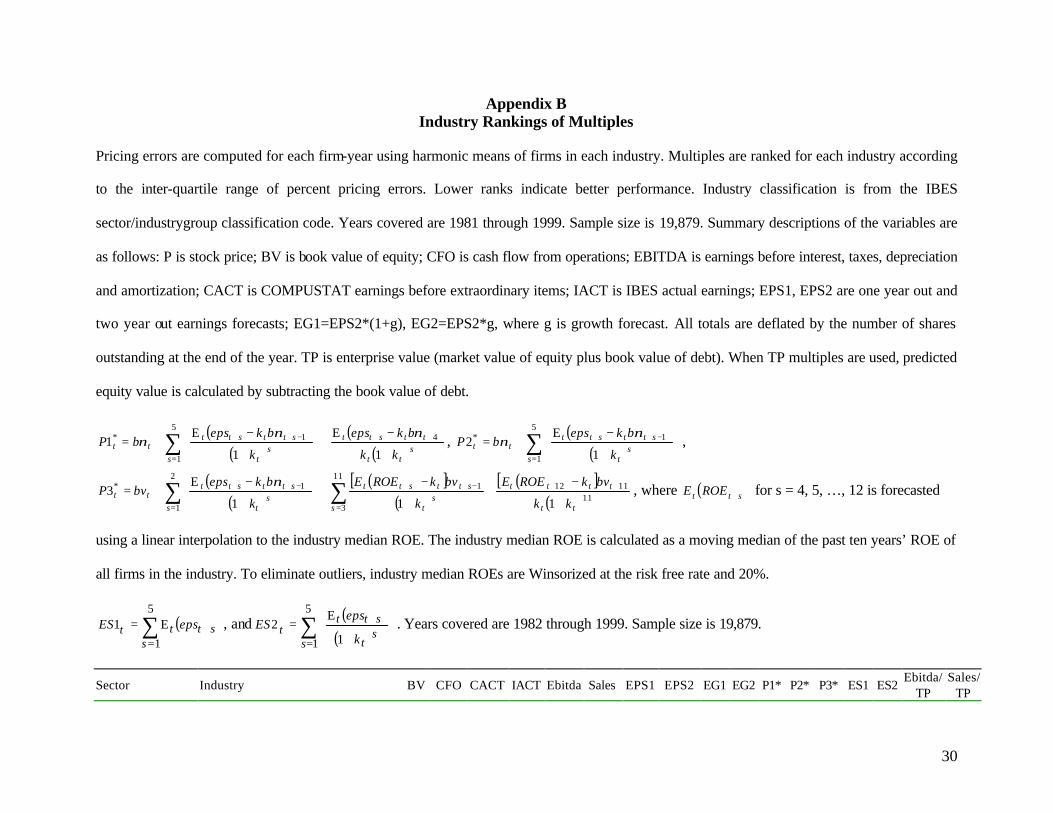
Appendix B Industry Rankings of Multiples

Pricing errors are computed for each firm-year using harmonic means of firms in each industry. Multiples are ranked for each industry according

to the inter-quartile range of percent pricing errors. Lower ranks indicate better performance. Industry classification is from the IBES

sector/industrygroup classification code. Years covered are 1981 through 1999. Sample size is 19,879. Summary descriptions of the variables are

as follows: P is stock price; BV is book value of equity; CFO is cash flow from operations; EBITDA is earnings before interest, taxes, depreciation

and amortization; CACT is COMPUSTAT earnings before extraordinary items; IACT is IBES actual earnings; EPS1, EPS2 are one year out and

two year out earnings forecasts; EG1=EPS2*(1+g), EG2=EPS2*g, where g is growth forecast. All totals are deflated by the number of shares

outstanding at the end of the year. TP is enterprise value (market value of equity plus book value of debt). When TP multiples are used, predicted

equity value is calculated by subtracting the book value of debt.

( )( )

( )( )s

tt

ttstt

ss

t

sttstttt

kk

bkeps

k

bkepsbP

+

−+

+

−+= ++

=

−++∗ ∑1

E

1

E1 4

5

1

1 ννν ,

( )( )∑

=

−++∗

+

−+=

5

1

1

1

E2

ss

t

sttstttt

k

bkepsbP

νν ,

( )( )

( )[ ]( )

( )[ ]( )11

111211

3

12

1

1

111

E3

tt

tttt

ss

t

sttstt

ss

t

sttstttt

kk

bvkROEE

k

bvkROEE

k

bkepsbvP

+

−+

+

−+

+

−+= ++

=

−++

=

−++∗ ∑∑ ν, where ( )stt ROEE + for s = 4, 5, …, 12 is forecasted

using a linear interpolation to the industry median ROE. The industry median ROE is calculated as a moving median of the past ten years’ ROE of

all firms in the industry. To eliminate outliers, industry median ROEs are Winsorized at the risk free rate and 20%.

( )∑=

+=5

1

E1

ssttt epsES , and

( )( )∑

=

+

+=

5

1 1

E2

ss

t

sttt

k

epsES . Years covered are 1982 through 1999. Sample size is 19,879.

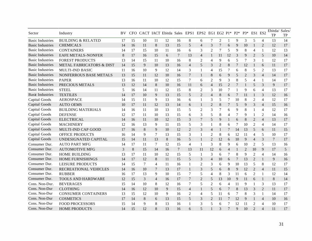
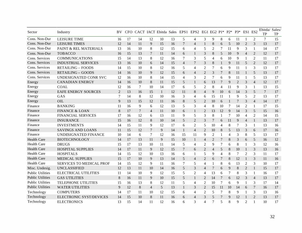
Sector Industry BV CFO CACT IACT Ebitda Sales EPS1 EPS2 EG1 EG2 P1* P2* P3* ES1 ES2 Ebitda/

TP Sales/

TP

31

Sector Industry BV CFO CACT IACT Ebitda Sales EPS1 EPS2 EG1 EG2 P1* P2* P3* ES1 ES2 Ebitda/

TP Sales/

TP Basic Industries BUILDING & RELATED 17 15 10 11 12 16 8 6 7 2 1 9 3 5 4 13 14 Basic Industries CHEMICALS 14 16 11 8 13 15 5 4 3 7 6 9 10 1 2 12 17 Basic Industries CONTAINERS 14 17 15 10 11 16 6 3 2 7 5 9 8 4 1 12 13 Basic Industries EAFE METALS-NONFER 8 17 16 15 6 7 13 4 1 11 12 3 9 2 5 10 14 Basic Industries FOREST PRODUCTS 13 14 15 11 10 16 8 2 4 9 6 5 7 3 1 12 17 Basic Industries METAL FABRICATORS & DIST 14 15 9 10 13 16 4 5 3 2 8 7 12 1 6 11 17 Basic Industries MULTI-IND BASIC 11 16 10 9 12 14 3 1 4 15 7 6 8 5 2 13 17 Basic Industries NONFERROUS BASE METALS 13 15 11 12 10 16 7 1 8 6 9 5 2 3 4 14 17 Basic Industries PAPER 13 16 11 10 12 15 7 6 2 9 3 8 5 4 1 14 17 Basic Industries PRECIOUS METALS 13 12 14 8 10 16 11 6 4 15 2 7 1 5 3 9 17 Basic Industries STEEL 5 16 14 11 12 15 8 2 3 10 7 1 9 6 4 13 17 Basic Industries TEXTILES 14 17 10 9 13 15 5 2 4 8 6 7 11 1 3 12 16 Capital Goods AEROSPACE 14 15 11 9 13 16 6 1 3 5 7 10 8 2 4 12 17 Capital Goods AUTO OEMS 10 17 11 12 13 14 6 1 2 8 7 5 9 3 4 15 16 Capital Goods BUILDING MATERIALS 14 16 11 10 13 15 5 2 3 7 6 9 8 1 4 12 17 Capital Goods DEFENSE 12 17 11 10 13 15 6 3 5 8 4 7 9 1 2 14 16 Capital Goods ELECTRICAL 14 16 11 10 12 15 3 7 5 9 1 6 8 2 4 13 17 Capital Goods MACHINERY 12 16 13 9 11 15 5 3 1 8 6 7 10 2 4 14 17 Capital Goods MULTI-IND CAP GOOD 17 16 8 9 10 12 2 3 4 1 7 14 13 5 6 11 15 Capital Goods OFFICE PRODUCTS 16 14 9 7 13 15 3 1 2 8 6 12 11 4 5 10 17 Capital Goods UNDESIGNATED CAPITAL 15 14 11 13 8 16 5 1 2 12 6 10 9 4 3 7 17 Consumer Dur. AUTO PART MFG 14 17 11 7 12 15 4 1 3 8 9 6 10 2 5 13 16 Consumer Dur. AUTOMOTIVE MFG 3 8 15 14 16 7 13 11 12 6 4 1 2 10 9 17 5 Consumer Dur. HOME BUILDING 13 17 11 10 12 15 5 1 3 6 7 8 9 2 4 14 16 Consumer Dur. HOME FURNISHINGS 14 17 12 8 11 15 5 3 4 10 6 7 13 2 1 9 16 Consumer Dur. LEISURE PRODUCTS 14 15 7 4 11 16 1 2 3 6 9 10 13 5 8 12 17 Consumer Dur. RECREATIONAL VEHICLES 14 16 10 7 13 17 1 3 5 6 8 9 12 2 4 11 15 Consumer Dur. RUBBER 16 17 13 9 10 15 7 5 4 8 3 11 6 2 1 12 14 Consumer Dur. TOOLS AND HARDWARE 12 15 3 4 16 17 7 2 5 13 10 9 11 6 1 8 14 Cons. Non-Dur. BEVERAGES 15 14 10 8 12 16 7 5 2 6 4 11 9 1 3 13 17 Cons. Non-Dur CLOTHING 14 16 12 10 9 15 4 1 5 6 7 8 13 3 2 11 17 Cons. Non-Dur CONSUMER CONTAINERS 13 15 12 10 9 16 2 4 5 11 6 7 8 3 1 14 17 Cons. Non-Dur COSMETICS 17 14 8 6 13 15 5 3 2 11 7 12 9 1 4 10 16 Cons. Non-Dur FOOD PROCESSORS 15 14 9 8 13 16 1 3 5 6 7 12 11 2 4 10 17 Cons. Non-Dur HOME PRODUCTS 14 15 12 8 13 16 6 5 1 3 7 9 10 2 4 11 17

32

Sector Industry BV CFO CACT IACT Ebitda Sales EPS1 EPS2 EG1 EG2 P1* P2* P3* ES1 ES2 Ebitda/

TP Sales/

TP Cons. Non-Dur LEISURE TIME 16 17 14 12 10 13 5 4 3 9 8 6 11 1 2 7 15 Cons. Non-Dur LEISURE TIMES 12 14 11 9 15 16 7 4 1 8 6 5 10 2 3 13 17 Cons. Non-Dur PAINT & REL MATERIALS 13 16 10 8 12 15 6 4 5 2 7 11 9 3 1 14 17 Cons. Non-Dur TOBACCO 16 15 13 7 11 14 6 1 3 8 5 10 9 4 2 12 17 Cons. Services COMMUNICATIONS 15 14 13 8 12 16 7 3 5 4 6 10 9 1 2 11 17 Cons. Services INDUSTRIAL SERVICES 13 16 10 6 14 15 4 7 3 8 1 9 11 5 2 12 17 Cons. Services RETAILING – FOODS 14 15 10 8 12 16 5 4 2 7 6 9 11 1 3 13 17 Cons. Services RETAILING – GOODS 14 16 10 9 12 15 6 4 2 3 7 8 11 1 5 13 17 Cons. Services UNDESIGNATED CONR SVC 12 16 10 8 14 15 4 3 2 7 6 9 11 1 5 13 17 Energy CANADIAN ENERGY 14 16 10 8 11 15 5 1 6 13 7 9 2 3 4 12 17 Energy COAL 12 16 7 10 14 17 6 5 2 8 4 11 9 3 1 13 15 Energy EAFE ENERGY SOURCES 2 13 16 15 1 12 11 8 4 9 10 6 14 3 5 7 17 Energy GAS 7 14 8 12 10 16 3 4 6 15 11 1 9 5 2 13 17 Energy OIL 9 13 15 12 11 16 8 5 2 10 6 1 7 3 4 14 17 Finance BANKING 11 16 9 6 12 13 5 3 4 8 10 7 14 2 1 17 15 Finance FINANCE & LOAN 8 17 7 4 11 10 6 1 2 13 12 9 14 3 5 15 16 Finance FINANCIAL SERVICES 17 16 12 6 13 11 9 5 3 8 1 7 10 4 2 14 15 Finance INSURANCE 15 16 12 8 10 14 5 2 3 7 6 11 9 4 1 13 17 Finance INVESTMENTS 14 15 11 9 12 17 6 2 5 10 4 8 7 3 1 13 16 Finance SAVINGS AND LOANS 11 15 12 7 9 14 1 4 2 10 8 5 13 3 6 17 16 Finance UNDESIGNATED FINANCE 10 14 6 7 12 16 15 11 9 2 1 4 3 8 5 13 17 Health Care BIOTECHNOLOGY 14 17 13 11 9 15 10 1 4 2 7 8 3 6 5 16 12 Health Care DRUGS 15 17 13 10 11 14 5 4 2 9 7 6 8 1 3 12 16 Health Care HOSPITAL SUPPLIES 14 17 11 9 12 15 7 6 2 4 5 8 10 1 3 13 16 Health Care HOSPITALS 14 15 12 10 13 16 6 1 5 9 4 8 7 2 3 11 17 Health Care MEDICAL SUPPLIES 15 17 10 9 13 14 5 4 2 6 7 8 12 1 3 11 16 Health Care SERVICES TO MEDICAL PROF 14 15 12 9 11 16 7 5 4 1 8 6 13 2 3 10 17 Misc. Undesig. UNCLASSIFIED 12 13 11 10 14 16 5 3 4 7 6 9 8 2 1 15 17 Public Utilities ELECTRICAL UTILITIES 11 14 10 9 12 15 5 2 4 13 6 7 8 3 1 16 17 Public Utilities GAS UTILITIES 8 16 11 9 10 15 5 1 2 14 7 6 12 3 4 13 17 Public Utilities TELEPHONE UTILITIES 15 16 13 8 12 11 5 4 2 10 7 6 9 1 3 17 14 Public Utilities WATER UTILITIES 9 12 8 4 5 13 1 3 2 15 11 10 14 6 7 16 17 Technology COMPUTERS 14 17 11 10 12 15 6 4 2 5 7 8 9 1 3 13 16 Technology ELECTRONIC SYST/DEVICES 14 15 10 8 11 16 6 4 3 5 7 9 12 1 2 13 17 Technology ELECTRONICS 13 15 14 11 12 16 6 3 4 7 5 8 9 2 1 10 17

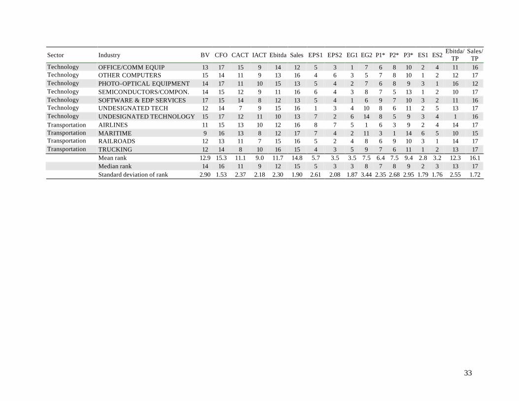
33

Sector Industry BV CFO CACT IACT Ebitda Sales EPS1 EPS2 EG1 EG2 P1* P2* P3* ES1 ES2 Ebitda/

TP Sales/

TP Technology OFFICE/COMM EQUIP 13 17 15 9 14 12 5 3 1 7 6 8 10 2 4 11 16 Technology OTHER COMPUTERS 15 14 11 9 13 16 4 6 3 5 7 8 10 1 2 12 17 Technology PHOTO-OPTICAL EQUIPMENT 14 17 11 10 15 13 5 4 2 7 6 8 9 3 1 16 12 Technology SEMICONDUCTORS/COMPON. 14 15 12 9 11 16 6 4 3 8 7 5 13 1 2 10 17 Technology SOFTWARE & EDP SERVICES 17 15 14 8 12 13 5 4 1 6 9 7 10 3 2 11 16 Technology UNDESIGNATED TECH 12 14 7 9 15 16 1 3 4 10 8 6 11 2 5 13 17 Technology UNDESIGNATED TECHNOLOGY 15 17 12 11 10 13 7 2 6 14 8 5 9 3 4 1 16 Transportation AIRLINES 11 15 13 10 12 16 8 7 5 1 6 3 9 2 4 14 17 Transportation MARITIME 9 16 13 8 12 17 7 4 2 11 3 1 14 6 5 10 15 Transportation RAILROADS 12 13 11 7 15 16 5 2 4 8 6 9 10 3 1 14 17 Transportation TRUCKING 12 14 8 10 16 15 4 3 5 9 7 6 11 1 2 13 17 Mean rank 12.9 15.3 11.1 9.0 11.7 14.8 5.7 3.5 3.5 7.5 6.4 7.5 9.4 2.8 3.2 12.3 16.1 Median rank 14 16 11 9 12 15 5 3 3 8 7 8 9 2 3 13 17 Standard deviation of rank 2.90 1.53 2.37 2.18 2.30 1.90 2.61 2.08 1.87 3.44 2.35 2.68 2.95 1.79 1.76 2.55 1.72

34

REFERENCES

Abarbanell, J., and V. L. Bernard. “Is the U.S. stock market myopic?” Journal of Accounting Research,

(Autumn, 2000): 221–42

Alford, A. “The effect of the set of comparable firms on the accuracy of the price-earnings valuation

method,” Journal of Accounting Research 30 (1992): 94–108.

Baker, M. and R. Ruback. “Estimating Industry Multiples,” working paper, Harvard University,

Cambridge, MA. 1999.

Basu , S. “Investment performance of common stocks in relation to their price-earnings ratios: A test of

the efficient markets hypothesis.” Journal of Finance (1977): 663–682.

Beatty, R.P., S.M. Riffe, and R. Thompson. “The method of comparables and tax court valuations of

private firms: an empirical investigation,” Accounting Horizons 13 (1999): 177–199

Boatsman, J., Baskin, E. “Asset valuation with incomplete markets,” The Accounting Review 56 (1981):

38-53.

Bradshaw, M.T., “How do analysts use their earning forecasts in generating stock recommendations?”

Working paper, University of Michigan, Ann Arbor, MI. 1999a.

Bradshaw, M.T., “Analysts reports, target prices, and stock recommendations.” Working paper,

University of Michigan, Ann Arbor, MI. 1999b.

Cheng, C.S.A and R. McNamara. “The Valuation Accuracy of the Price-Earnings and Price-Book

Benchmark Valuation Methods.” Working paper, University of Houston, Houston, TX. 1996.

Claus, J. J. and J. K.Thomas. “Equity premia as low as three percent? Empirical evidence from analysts’

earnings forecasts for domestic and international stock markets.” Working paper, Columbia

University, New York, NY, 2000.

Copeland, T., Koller and Murrin. “Valuation.” Wiley. 1994.

Damodaran, A. “Damodaran on valuation.” Wiley. 1996.

Frankel, R. and C. M. C. Lee. “Accounting Valuation, Market Expectation, and cross-sectional stock

returns.” Journal of Accounting and Economics 25 (1998): 283–319.

35

Feltham, G. and J. A. Ohlson. "Valuation and Clean Surplus Accounting for Operating and Financial

Activities." Contemporary Accounting Research (Spring 1995): 689–731.

Gebhardt, W. R., C. M. C. Lee and B. Swaminathan. “Toward and ex ante cost-of-capital.” Journal of

Accounting Research (2001, forthcoming).

Gilson, S.C., Hotchkiss, E.S., Ruback, R.S. “Valuation of bankrupt firms.” Review of Financial Studies

13, (2000): 43–74.

Hand, J.R.M. “Profits, losses, and the stock of internet firms,” working paper, University of North

Carolina, Chapel Hill, NC. 1999.

Hand, J.R.M. “The role of economic fundamental, web traffic, and supply and demand in the pricing of

US internet stocks,” working paper, University of North Carolina, Chapel Hill, NC. 2000.

Kaplan, S. N. and R. S. Ruback. “The valuation of cash flow forecasts: An empirical analysis,” The

Journal of Finance 50 (1995): 1059–1093.

Kim, M. and J. Ritter, “Valuing IPOs,” forthcoming, Journal of Financial Economics 53 (1999): 409–37.

LeClair, M.S. “Valuing the closely-held corporation: the validity and performance of established

valuation procedures,” Accounting Horizons 4 (September, 1990) 31–42.

Liu, J. 1999. “Post-earnings-announcement Drift and Analyst Forecasts.” Working paper, UCLA, Los

Angeles, CA.

Liu, J. and J. Thomas. “Stock Returns and Accounting Earnings.” Journal of Accounting Research. 38

(Spring 2000): 71-101.

Liu, J., D. Nissim, and J. Thomas. “Valuations based on multiples and future stock returns,” Working

paper, Columbia University, New York, NY. 2001

Ohlson, J. "Earnings, Book Values, and Dividends in Equity Valuation," Contemporary Accounting

Research (spring 1995): 661–687.

Palepu, K, P. Healy, and V. Bernard. “Business analysis and valuation,” 2nd Edition, South-Western

College Publishing, 2000.

Penman, S.H.. “Financial Statement Analysis and Security Valuation”, McGraw-Hill Irwin, 2001.

36

Stattman, D. “Book value and stock returns.” The Chicago MBA: A Journal of selected papers.

University of Chicago, Chicago, IL., 1980, 25–45.

Tasker, S. C. “Industry preferred multiples in acquisition valuation,” working paper, Cornell University,

Ithaca, NY. 1998.

Trueman, B., M.H.F. Wong, and X. Zhang. “The eyeballs have it: searching for the value in internet

stocks”, working paper, University of California, Berkeley, CA, 2000.

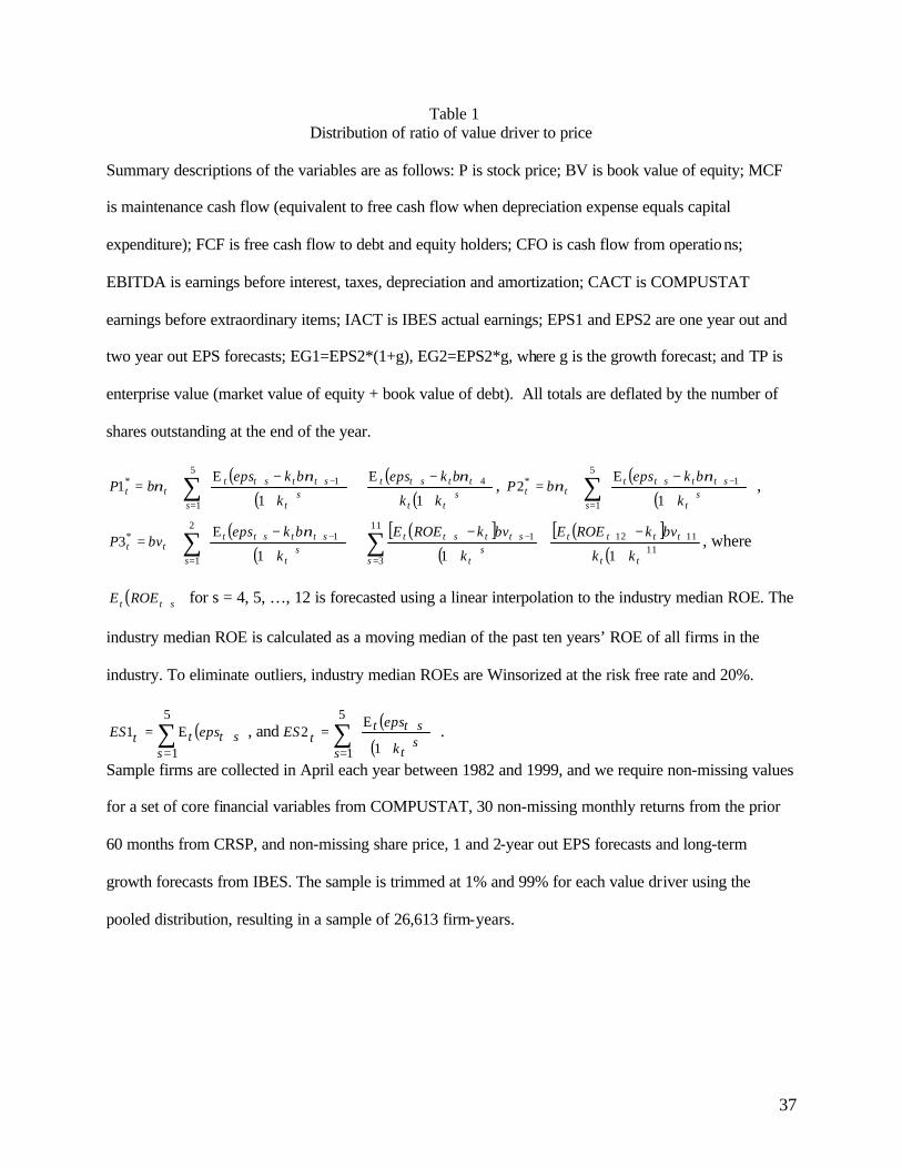
37

Table 1 Distribution of ratio of value driver to price

Summary descriptions of the variables are as follows: P is stock price; BV is book value of equity; MCF

is maintenance cash flow (equivalent to free cash flow when depreciation expense equals capital

expenditure); FCF is free cash flow to debt and equity holders; CFO is cash flow from operations;

EBITDA is earnings before interest, taxes, depreciation and amortization; CACT is COMPUSTAT

earnings before extraordinary items; IACT is IBES actual earnings; EPS1 and EPS2 are one year out and

two year out EPS forecasts; EG1=EPS2*(1+g), EG2=EPS2*g, where g is the growth forecast; and TP is

enterprise value (market value of equity + book value of debt). All totals are deflated by the number of

shares outstanding at the end of the year.

( )( )

( )( )s

tt

ttstt

ss

t

sttstttt

kk

bkeps

k

bkepsbP

+

−+

+

−+= ++

=

−++∗ ∑1

E

1

E1 4

5

1

1 ννν ,

( )( )∑

=

−++∗

+

−+=

5

1

1

1

E2

ss

t

sttstttt

k

bkepsbP

νν ,

( )( )

( )[ ]( )

( )[ ]( )11

111211

3

12

1

1

111

E3

tt

tttt

ss

t

sttstt

ss

t

sttstttt

kk

bvkROEE

k

bvkROEE

k

bkepsbvP

+

−+

+

−+

+

−+= ++

=

−++

=

−++∗ ∑∑ ν, where

( )stt ROEE + for s = 4, 5, …, 12 is forecasted using a linear interpolation to the industry median ROE. The

industry median ROE is calculated as a moving median of the past ten years’ ROE of all firms in the

industry. To eliminate outliers, industry median ROEs are Winsorized at the risk free rate and 20%.

( )∑=

+=5

1

E1

ssttt epsES , and

( )( )∑

=

+

+=

5

1 1

E2

ss

t

sttt

k

epsES .

Sample firms are collected in April each year between 1982 and 1999, and we require non-missing values

for a set of core financial variables from COMPUSTAT, 30 non-missing monthly returns from the prior

60 months from CRSP, and non-missing share price, 1 and 2-year out EPS forecasts and long-term

growth forecasts from IBES. The sample is trimmed at 1% and 99% for each value driver using the

pooled distribution, resulting in a sample of 26,613 firm-years.

38

Mean SD 1% 5% 10% 25% 50% 75% 90% 95% 99%

BV/P 0.549 0.336 0.050 0.131 0.184 0.308 0.489 0.717 0.985 1.180 1.620 MCF/P 0.035 0.183 -0.566 -0.171 -0.076 -0.002 0.035 0.074 0.145 0.238 0.626

FCF/P -0.025 0.252 -1.008 -0.379 -0.218 -0.069 0.002 0.050 0.131 0.234 0.648

CFO/P 0.093 0.190 -0.516 -0.100 -0.019 0.034 0.079 0.146 0.239 0.328 0.693

CACT/P 0.050 0.073 -0.249 -0.043 0.005 0.033 0.056 0.080 0.108 0.130 0.178

IACT/P 0.057 0.060 -0.184 -0.013 0.018 0.040 0.059 0.082 0.109 0.130 0.175

Ebitda/P 0.173 0.128 -0.051 0.032 0.055 0.095 0.148 0.224 0.320 0.397 0.617

Sales/P 1.419 1.416 0.098 0.215 0.313 0.552 0.988 1.773 2.991 4.080 7.112

EPS1/P 0.073 0.037 -0.026 0.024 0.036 0.052 0.070 0.092 0.117 0.137 0.178 EPS2/P 0.091 0.036 0.027 0.043 0.052 0.067 0.085 0.108 0.138 0.160 0.205

EG1/P 0.105 0.040 0.034 0.052 0.062 0.077 0.097 0.124 0.159 0.183 0.235

EG2/P 0.013 0.007 0.002 0.004 0.005 0.008 0.011 0.016 0.021 0.026 0.036

P1*/P 0.708 0.296 0.222 0.318 0.383 0.500 0.658 0.863 1.086 1.264 1.660

P2*/P 0.587 0.241 0.186 0.258 0.308 0.407 0.553 0.732 0.910 1.029 1.304

P3*/P 0.652 0.366 0.125 0.203 0.266 0.393 0.577 0.834 1.120 1.330 1.918

ES1/P 0.525 0.202 0.164 0.259 0.310 0.389 0.489 0.624 0.794 0.912 1.168 ES2/P 0.350 0.125 0.111 0.173 0.209 0.265 0.334 0.417 0.517 0.588 0.723

Ebitda/TP 0.113 0.060 -0.031 0.026 0.044 0.075 0.110 0.147 0.187 0.215 0.276

Sales/TP 0.939 0.788 0.086 0.169 0.234 0.396 0.708 1.234 1.925 2.495 3.981

39

Table 2 Distribution of pricing errors for simple multiples

Value and value drivers are assumed to be proportional: itittit xp εβ += . Multiples are estimated using

harmonic means:

=

it

ittt p

xE1β in Panels A&B, and medians are used in Panel C. Pricing error is

it

itit

it

it

p

xp

p

^

βε −= Summary descriptions of the variables are as follows: P is stock price; BV is book value

of equity; CFO is cash flow from operations; EBITDA is earnings before interest, taxes, depreciation and

amortization; CACT is COMPUSTAT earnings before extraordinary items; IACT is IBES actual

earnings; EPS1, EPS2 are one year out and two year out EPS forecasts; EG1=EPS2*(1+g), EG2=EPS2*g,

where g is growth forecast. All totals are deflated by the number of shares outstanding at the end of the

year. TP is enterprise value (market value of equity plus book value of debt). When TP multiples are

used, predicted equity value is calculated by subtracting the book value of debt.

( )( )

( )( )s

tt

ttstt

ss

t

sttstttt

kk

bkeps

k

bkepsbP

+

−+

+

−+= ++

=

−++∗ ∑1

E

1

E1 4

5

1

1 ννν ,

( )( )∑

=

−++∗

+

−+=

5

1

1

1

E2

ss

t

sttstttt

k

bkepsbP

νν ,

( )( )

( )[ ]( )

( )[ ]( )11

111211

3

12

1

1

111

E3

tt

tttt

ss

t

sttstt

ss

t

sttstttt

kk

bvkROEE

k

bvkROEE

k

bkepsbvP

+

−+

+

−+

+

−+= ++

=

−++

=

−++∗ ∑∑ ν, where

( )stt ROEE + for s = 4, 5, …, 12 is forecasted using a linear interpolation to the industry median ROE. The

industry median ROE is calculated as a moving median of the past ten years’ ROE of all firms in the

industry. To eliminate outliers, industry median ROEs are Winsorized at the risk free rate and 20%.

( )∑=

+=5

1

E1

ssttt epsES , and

( )( )∑

=

+

+=

5

1 1

E2

ss

t

sttt

k

epsES . Sample firms are collected in April each year

between 1982 and 1999, and we require non-missing values for a set of core financial variables from

COMPUSTAT, 30 non-missing monthly returns from the prior 60 months from CRSP, and non-missing

share price, 1 and 2-year out EPS forecasts and long-term growth forecasts from IBES. The sample is

trimmed at 1% and 99% for each value driver. We then require a minimum $2 share price, that all value

drivers be positive, and that each industry-year combination have at least five observations. The final

sample contains 19,879 firm-years.

40

Panel A: Multiples based on harmonic means of firms from the same industry

Mean Median SD 75%-25% 90%-10% 95%-5% BV/P -0.016 0.066 0.560 0.602 1.266 1.710

CFO/P -0.042 0.150 0.989 0.777 1.652 2.355 CACT/P -0.012 0.012 0.490 0.518 1.119 1.549

IACT/P -0.009 0.023 0.421 0.442 0.941 1.317

Ebitda/P -0.017 0.066 0.573 0.553 1.163 1.631

Sales/P -0.032 0.163 0.859 0.738 1.645 2.357

EPS1/P -0.005 0.015 0.321 0.348 0.744 1.037

EPS2/P -0.004 0.021 0.290 0.317 0.677 0.935

EG1/P -0.004 0.027 0.290 0.313 0.671 0.936

EG2/P -0.009 0.071 0.435 0.424 0.907 1.280

P1*/P -0.006 0.037 0.351 0.377 0.807 1.118 P2*/P -0.006 0.033 0.352 0.410 0.835 1.124

P3*/P -0.009 0.055 0.443 0.469 0.983 1.377

ES1/P -0.004 0.026 0.285 0.307 0.661 0.915

ES2/P -0.004 0.023 0.283 0.311 0.664 0.919

Ebitda/TP -0.013 0.024 0.645 0.619 1.266 1.753 Sales/TP -0.057 0.156 1.067 0.901 1.919 2.763

Panel B: Multiples based on harmonic means of firms from the entire cross-section

Mean Median SD 75%-25% 90%-10% 95%-5% BV/P 0.000 0.080 0.565 0.744 1.343 1.732

CFO/P -0.001 0.261 1.086 0.812 1.682 2.460

CACT/P 0.000 0.045 0.512 0.625 1.228 1.627 IACT/P 0.000 0.048 0.453 0.551 1.077 1.431

Ebitda/P 0.000 0.127 0.613 0.692 1.343 1.778

Sales/P -0.001 0.265 0.943 0.801 1.766 2.531

EPS1/P 0.000 0.028 0.361 0.452 0.880 1.166

EPS2/P 0.000 0.030 0.320 0.388 0.781 1.038

EG1/P 0.000 0.041 0.317 0.368 0.754 1.024

EG2/P 0.000 0.077 0.500 0.526 1.168 1.608

P1*/P 0.000 0.053 0.378 0.479 0.923 1.211 P2*/P 0.000 0.052 0.396 0.549 0.986 1.250

P3*/P 0.000 0.098 0.511 0.652 1.257 1.587

ES1/P 0.000 0.040 0.312 0.362 0.740 1.008

ES2/P 0.000 0.030 0.312 0.379 0.760 1.011

Ebitda/TP -0.008 0.029 0.734 0.704 1.415 1.939 Sales/TP 0.026 0.284 1.337 1.097 2.374 3.648

41

Panel C: Multiples based on median of comparable firms from the same industry

Mean Median SD 75%-25% 90%-10% 95%-5% BV/P -0.110 0.000 0.638 0.649 1.407 1.962

CFO/P -0.263 0.000 1.235 0.903 2.020 2.944 CACT/P -0.041 0.000 0.527 0.513 1.164 1.640

IACT/P -0.046 0.000 0.457 0.450 0.985 1.394

Ebitda/P -0.111 0.000 0.676 0.581 1.283 1.814

Sales/P -0.287 0.001 1.157 0.887 2.062 3.020

EPS1/P -0.028 -0.001 0.351 0.350 0.761 1.074

EPS2/P -0.033 0.000 0.314 0.320 0.696 0.980

EG1/P -0.039 0.000 0.318 0.318 0.702 0.982

EG2/P -0.099 -0.003 0.490 0.444 0.988 1.419

P1*/P 0.014 0.029 0.441 0.425 0.982 1.604 P2*/P -0.051 0.000 0.378 0.421 0.882 1.205

P3*/P -0.087 0.000 0.497 0.499 1.070 1.522

ES1/P -0.039 0.000 0.312 0.312 0.691 0.967

ES2/P -0.035 0.000 0.306 0.319 0.691 0.961

Ebitda/TP -0.054 0.000 0.678 0.629 1.321 1.842 Sales/TP -0.290 0.000 1.312 1.038 2.279 3.361

42

Table 3 Distribution of pricing errors for intercept adjusted multiples

Value and value drivers are assumed to be linear: ititttit xp εβα ++= . Multiple is estimated excluding the

firm under valuation, by solving the following constrained minimization problem:

]]/)var[()/( varmin,

ititttititit pxpp ⋅−−= βαεβα

; .0E .. =

it

it

pts

ε Pricing error is it

itttit

it

it

p

xp

p

^^

βαε −−=

Summary descriptions of the variables are as follows: P is stock price; BV is book value of equity; CFO is

cash flow from operations; EBITDA is earnings before interest, taxes, depreciation and amortization;

CACT is COMPUSTAT earnings before extraordinary items; IACT is IBES actual earnings; EPS1, EPS2

are one year out and two year out EPS forecasts; EG1=EPS2*(1+g), EG2=EPS2*g, where g is growth

forecast. All totals are deflated by the number of shares outstanding at the end of the year. TP is enterprise

value (market value of equity plus book value of debt). When TP multiples are used, predicted equity

value is calculated by subtracting the book value of debt.

( )( )

( )( )s

tt

ttstt

ss

t

sttstttt

kk

bkeps

k

bkepsbP

+

−+

+

−+= ++

=

−++∗ ∑1

E

1

E1 4

5

1

1 ννν ,

( )( )∑

=

−++∗

+

−+=

5

1

1

1

E2

ss

t

sttstttt

k

bkepsbP

νν ,

( )( )

( )[ ]( )

( )[ ]( )11

111211

3

12

1

1

111

E3

tt

tttt

ss

t

sttstt

ss

t

sttstttt

kk

bvkROEE

k

bvkROEE

k

bkepsbvP

+

−+

+

−+

+

−+= ++

=

−++

=

−++∗ ∑∑ ν, where

( )stt ROEE + for s = 4, 5, …, 12 is forecasted using a linear interpolation to the industry median ROE. The

industry median ROE is calculated as a moving median of the past ten years’ ROE of all firms in the

industry. To eliminate outliers, industry median ROEs are Winsorized at the risk free rate and 20%.

( )∑=

+=5

1

E1

ssttt epsES , and

( )( )∑

=

+

+=

5

1 1

E2

ss

t

sttt

k

epsES .

Sample firms are collected in April each year between 1982 and 1999, and we require non-missing values

for a set of core financial variables from COMPUSTAT, 30 non-missing monthly returns from the prior

60 months from CRSP, and non-missing share price, 1 and 2-year out EPS forecasts and long-term

growth forecasts from IBES. The sample is trimmed at 1% and 99% for each value driver. We then

require a minimum $2 share price, that all value drivers be positive, and that each industry-year

combination have at least five observations. The final sample contains 19,879 firm-years.

43

Panel A: Comparable firms from the same industry

Mean Median SD 75%-25% 90%-10% 95%-5% BV/P -0.027 0.058 0.538 0.538 1.153 1.599

CFO/P -0.037 0.091 0.621 0.577 1.237 1.765 CACT/P -0.018 0.027 0.439 0.433 0.953 1.352

IACT/P -0.015 0.029 0.387 0.390 0.843 1.179

Ebitda/P -0.025 0.052 0.488 0.482 1.041 1.459

Sales/P -0.039 0.101 0.646 0.614 1.312 1.841

EPS1/P -0.010 0.018 0.310 0.323 0.704 0.982

EPS2/P -0.008 0.019 0.290 0.305 0.656 0.917

EG1/P -0.007 0.023 0.291 0.306 0.654 0.912

EG2/P -0.012 0.055 0.400 0.402 0.855 1.195

P1*/P -0.013 0.034 0.348 0.365 0.775 1.078 P2*/P -0.014 0.028 0.360 0.392 0.819 1.120

P3*/P -0.020 0.045 0.428 0.433 0.919 1.276

ES1/P -0.007 0.022 0.285 0.301 0.648 0.888

ES2/P -0.007 0.021 0.283 0.302 0.649 0.891

Ebitda/TP -0.008 0.025 0.626 0.538 1.121 1.576 Sales/TP -0.038 0.094 0.838 0.730 1.532 2.154

Panel B: Comparable firms from the entire cross-section

Mean Median SD 75%-25% 90%-10% 95%-5% BV/P 0.008 0.084 0.518 0.610 1.171 1.581

CFO/P 0.013 0.175 0.654 0.582 1.279 1.833

CACT/P -0.002 0.053 0.447 0.513 1.006 1.385 IACT/P -0.005 0.050 0.405 0.475 0.923 1.252

Ebitda/P 0.012 0.111 0.517 0.560 1.090 1.513

Sales/P 0.038 0.206 0.646 0.595 1.293 1.849

EPS1/P -0.009 0.025 0.339 0.415 0.811 1.092

EPS2/P -0.007 0.023 0.315 0.376 0.759 1.024

EG1/P -0.003 0.040 0.314 0.361 0.743 1.016

EG2/P 0.031 0.120 0.459 0.495 1.060 1.459

P1*/P -0.007 0.049 0.359 0.445 0.855 1.141 P2*/P -0.007 0.042 0.385 0.517 0.934 1.200

P3*/P -0.010 0.078 0.455 0.556 1.047 1.380

ES1/P -0.002 0.040 0.308 0.355 0.732 0.993

ES2/P -0.006 0.028 0.307 0.366 0.739 0.994

Ebitda/TP 0.044 0.059 0.686 0.587 1.207 1.710 Sales/TP 0.143 0.246 1.010 0.835 1.860 2.805

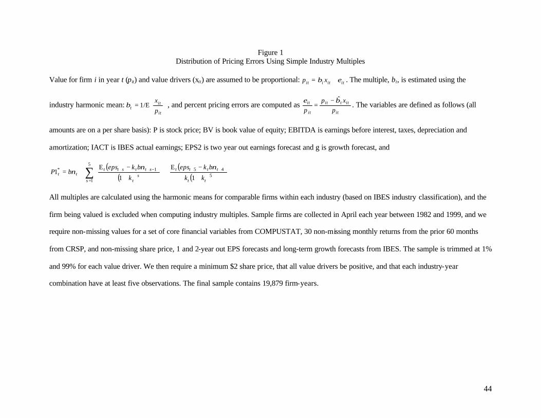
44

Figure 1 Distribution of Pricing Errors Using Simple Industry Multiples

Value for firm i in year t (pit) and value drivers (xit) are assumed to be proportional: ititiit xp εβ += . The multiple, βt, is estimated using the

industry harmonic mean:

=

it

itt p

x/E1β , and percent pricing errors are computed as

it

ittit

it

it

p

xp

p

βε ˆ−= . The variables are defined as follows (all

amounts are on a per share basis): P is stock price; BV is book value of equity; EBITDA is earnings before interest, taxes, depreciation and

amortization; IACT is IBES actual earnings; EPS2 is two year out earnings forecast and g is growth forecast, and

( )( )

( )( )∑

=

++−++∗

+

−+

+

−+=

5

15

451

1

E

1

E1

s tt

tttts

t

sttstttt

kk

bkeps

k

bkepsbP

ννν

All multiples are calculated using the harmonic means for comparable firms within each industry (based on IBES industry classification), and the

firm being valued is excluded when computing industry multiples. Sample firms are collected in April each year between 1982 and 1999, and we

require non-missing values for a set of core financial variables from COMPUSTAT, 30 non-missing monthly returns from the prior 60 months

from CRSP, and non-missing share price, 1 and 2-year out EPS forecasts and long-term growth forecasts from IBES. The sample is trimmed at 1%

and 99% for each value driver. We then require a minimum $2 share price, that all value drivers be positive, and that each industry-year

combination have at least five observations. The final sample contains 19,879 firm-years.

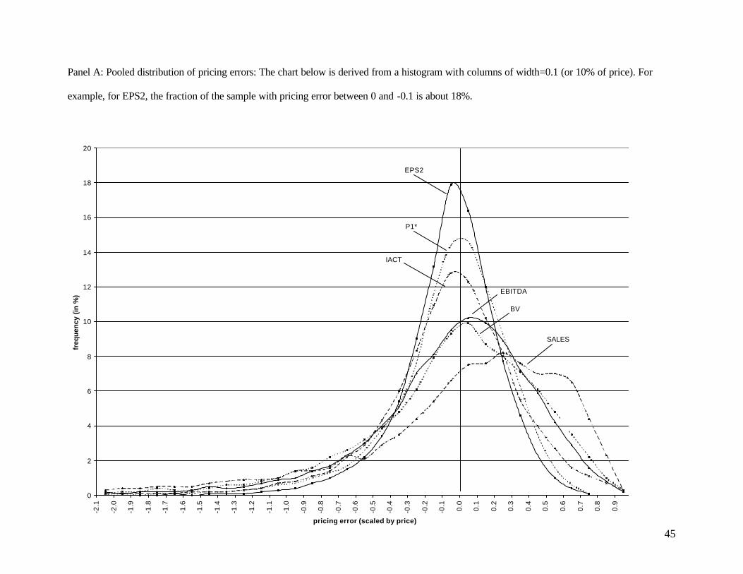
45

Panel A: Pooled distribution of pricing errors: The chart below is derived from a histogram with columns of width=0.1 (or 10% of price). For

example, for EPS2, the fraction of the sample with pricing error between 0 and -0.1 is about 18%.

0

2

4

6

8

10

12

14

16

18

20

-2.1

-2.0

-1.9

-1.8

-1.7

-1.6

-1.5

-1.4

-1.3

-1.2

-1.1

-1.0

-0.9

-0.8

-0.7

-0.6

-0.5

-0.4

-0.3

-0.2

-0.1 0.0

0.1

0.2

0.3

0.4

0.5

0.6

0.7

0.8

0.9

1.0

pricing error (scaled by price)

freq

uen

cy (

in %

)

BV

EPS2

IACT

SALES

EBITDA

P1*

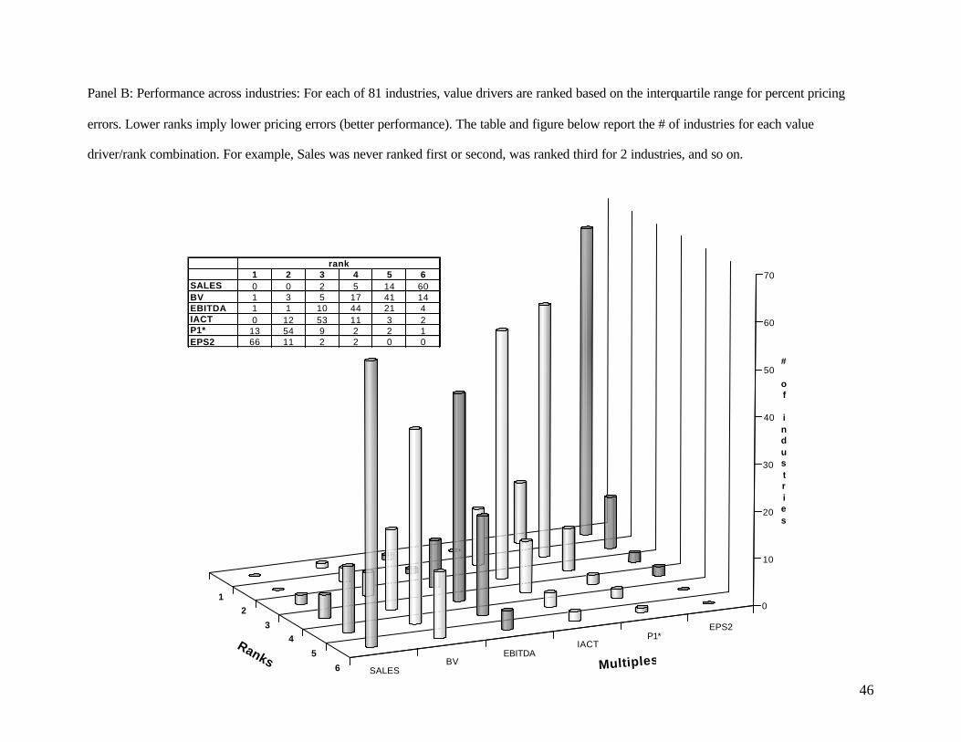
46

Panel B: Performance across industries: For each of 81 industries, value drivers are ranked based on the interquartile range for percent pricing

errors. Lower ranks imply lower pricing errors (better performance). The table and figure below report the # of industries for each value

driver/rank combination. For example, Sales was never ranked first or second, was ranked third for 2 industries, and so on.

12

34

5

6 SALESBV

EBITDAIACT

P1*EPS2

0

10

20

30

40

50

60

70

# of industries

Ranks Multiples

1 2 3 4 5 6SALES 0 0 2 5 14 60BV 1 3 5 17 41 14EBITDA 1 1 10 44 21 4IACT 0 12 53 11 3 2P1* 13 54 9 2 2 1EPS2 66 11 2 2 0 0

rank

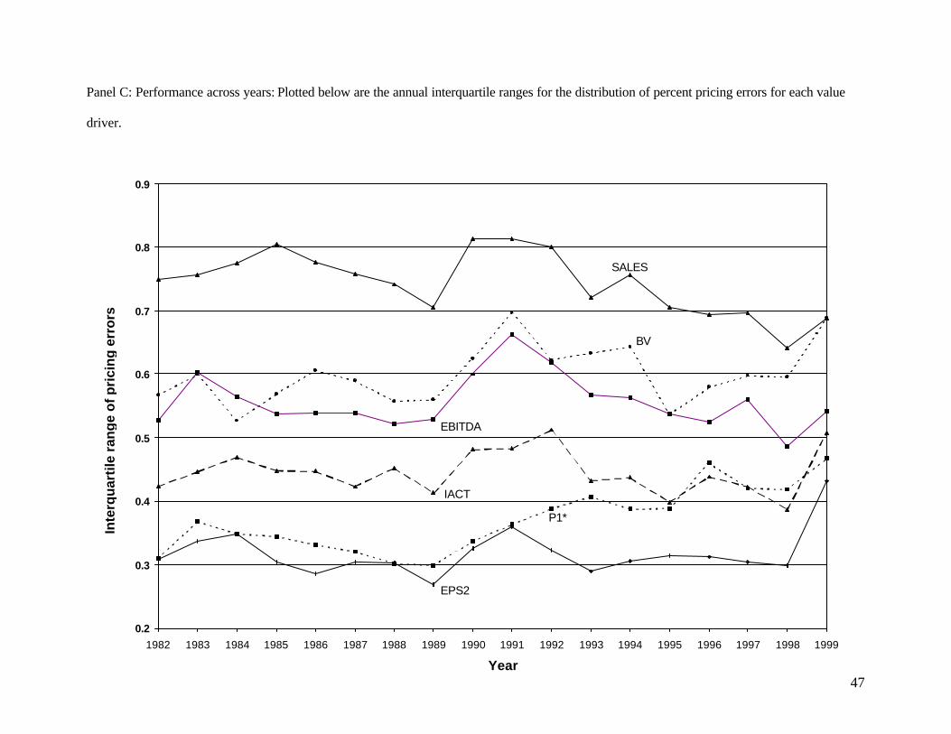
47

Panel C: Performance across years: Plotted below are the annual interquartile ranges for the distribution of percent pricing errors for each value

driver.

0.2

0.3

0.4

0.5

0.6

0.7

0.8

0.9

1982 1983 1984 1985 1986 1987 1988 1989 1990 1991 1992 1993 1994 1995 1996 1997 1998 1999

EPS2

SALES

BV

EBITDA

IACT

P1*

Inte

rqu

arti

le r

ang

e o

f p

rici

ng

err

ors

Year