environmental turbulence in the credit union...

Advances in Methodology, Data Analysis, and StatisticsAnuška Ferligoj (Editor), Metodološki zvezki, 14Ljubljana : FDV, 1998

Environmental Turbulence in the CreditUnion Industry : A Multiple Correspondence

Analysis Approach

Vlado Dimovski and Joe Rovan'

Abstract

Recent development of strategic management has proven that classicalmethodology for measuring the environment in terms of complexity,munificence, and dynamism (Dess and Beard, 1984) is unsuitable for one-industry studies (Dimovski, 1994) . Instead, as in this paper, an expanded andrefined measure of perceived environmental turbulence has been adopted andoperationalised . One of the techniques that can further verify the perceivedenvironmental turbulence construct is the multiple correspondence analysis(MCA) that has been used in this paper .

An investigation has been conducted on the population of credit unions inOhio, USA . Construct of perceived environmental turbulence has beenoperationalised by five variables designated as different aspects ofenvironmental turbulence (level of competitiveness within the industry, rate ofservices absolence, predictability of the competitors, predictability of consumerpreferences, service/product technology changes) . Variables are ordinal andhave been measured on a five-point Likert scale .

Using MCA the original five-dimensional variable space has been reducedto a two-dimensional subspace explaining about 58% of the total variance . Thecategories of the investigated variables have been represented as points in thetwo-dimensional map according to the values of the first two principalcoordinates . Given the ordinal nature of the variables used, it was meaningfulto connect the points belonging to the same variable .

The map shows a bi-polarization with most of the points representingcategories with low level of environmental turbulence on one side and with highlevel of environmental turbulence on the other side . The general orientation ofthe majority of connecting lines on the graph is parallel to the first principalaxis .

The parallel pattern of the connecting lines supports our initial hypothesisof having strong relationships among the variables of environmental turbulence .Such a result can also imply that most of the analysed variables measure thedegree of environmental turbulence .

I Faculty of Economics, University of Ljubljana, Kardeljeva pl . 17, 1109, Ljubljana, Slovenia

50

Vlado Dimovski and Joie Rovan

1 Introduction

The main purpose of this paper is to investigate the environmental turbulence and itsimpact on internal organisational processes and their adjustments to the environment .In the first part of the paper, we introduce the construct of environmental turbulenceand its operationalization by constructing variables that represent different aspects ofenvironmental turbulence . Then, to further verify the proposed construct multiplecorrespondence analysis (MCA) has been used . The results of MCA improve theinterpretation of environmental turbulence and illustrate how to use MCA forstrategic management field research .

2 Measuring environmental turbulence

The environment is broadly defined as a residual category of "everything else" butthe organisation (Thompson, 1967) . The environment is generally classified intomacroenvironment, industry-specific environment, and firm-specific environment(Glazer, 1990) .

The macroenvironment can have a significant impact on industry andorganisations, and includes an almost limitless variety of potentially importantfactors . These factors can be summarised into five major forces : regulatory,economic, global, social, and technological (Reimann, 1987) . The industry-specificenvironment has three major dimensions: munificence, dynamism, and complexity(Dess and Beard, 1984) . Environmental munificence is the extent to which theenvironment can support sustained growth . This means that organisations search forthe environments that provide opportunities for growth and stability (Day, 1977) .Environmental dynamism relates to environmental stability-instability characteristics(Miles, Snow, and Pfeffer, 1974) . Environmental complexity reflects theheterogeneity of organisational activities and their range (Tung, 1979) . The firm-specific environment consists of "market attractiveness," such as location, size,market share, and product life-cycle (Glazer, 1990) . The latter is an importantconcept due to its presence of information inflows .

The changes and riskiness of macroenvironment and industry-specificenvironment can force organisations to adjust by translating the environmentalchanges to the various processes in organisations and to individuals in organisations .Such changes can be referred to as environmental turbulence (Fiol and Lyles, 1985)which is also defined as "more events per unit time" (Glazer, 1990, p .7) . A turbulentenvironment requires larger scales and more intensive internal organisationalprocesses such as information acquisition and information interpretation particularlydue to a higher rate of organisational changes and riskiness .

Environmental Turbulence in the Credit Union Industry

5 1

3 Operationalisation of the environmental turbulenceconstruct

As Cool and Schendel point out the operationalisation of the construct underobservation "is always a function of industry under study" (Cool and Schendel, 1988,p.212) . For this paper the credit union industry was selected 2 .

Credit unions are not-for-profit organisations in which members who are also theowners share a common bond in depositing funds and obtaining credit . The uniquefeature of credit unions is this common bond . The bond is usually the place ofemployment or the occupation of the members (occupational bond) but it can also bebased on association ties, such as church or union membership (associational bond),or area of residency (community bond) .

One possible approach in operationalisation of environmental turbulence in termsof dynamism, munificence, and complexity has been proven unsuitable for one-industry studies (Dimovski, 1994) . Therefore, a different approach has been taken byoperationalising environmental turbulence as a measure with various aspects ofperceived environmental turbulence . The aspects of environmental turbulence : levelof competitiveness within the industry, rate of services absolence, predictability ofthe competitors, predictability of consumer preferences and service/producttechnology changes serve as a basis for items of research instrument - questionnaire .We combined the questions that have been developed for other studies as well as ourown questions originally developed for this study . Finally, a five-item questionnairewas used, where each of the variable is ordinal and has been measured on a five-pointLikert scale.

4 Data collection

The questionnaire was sent to 200 credit unions in Ohio, USA. This sample wasselected through a stratified sampling procedure with the size of credit union used asthe stratification criterion . After collecting the data (response rate was 42.5%), thequestionnaire was submitted to validity and reliability assessment. The validity

2 The reasons for selecting the credit union industry were the following :(a) it is a fast growing service-related industry with an expanding range of offered

services ;(b) the consumer banking market in which credit unions operate requires a high level

of adaptability to external change and a high level of alertness to environmentalinformation ;

(c)

not-for-profit organizations are "one of the most fruitful areas for researchingstrategic management" (Wortman, 1979, p .353) ;

(d) prior surveys indicate a high level of cooperativeness of general managers andCEOs of credit unions (Reichert and Rubens, 1994) ; and

(e)

detailed data bases are available through Ferguson and company .

52

V/ado Dimovski and Joie Rovan

assessment includes construct validity and assessment of reliability that was tested byusing Cronbach's alpha (alpha value was 0 .858) .

Construct validity' is a degree to which a construct achieves theoretical andempirical meaning. For construct validity we used factor analysis with loadings morethan 0 .45 considered adequate for establishing convergent validity . Those variablesthat fullfiled these criteria were used in our MCA .

The observed univariate distributions of the five variables are given in Table I .The univariate frequency distributions show that the categories D1 and El containonly one observation . For that reason these two categories were included into thefollowing categories D2 and E2 in MCA .

Table 1 : Indicate your degree of agreement or disagreement with the following statementsthat refer to actual conditions in the credit union industry .

Questions

(aspects of environmental turbulence )

A. Our credit union must change itsmarketing practices frequently to keepup with market competitors

B. The rate at which new services aregetting obsolete is very high

C . Actions of competitors areunpredictable

D. Demand and consumer preferences areunpredictable

E. The service/product technologychanges very frequently

5 Burt table

MCA can be defined as the CA of the so-called "Burt table" . It is a partitionedsymmetric matrix containing all pairs of crosstabulations among a set of categoricalvariables . Each crosstabulation F99 (q=1,2, . . .,Q) on the diagonal is a diagonal matrixof the marginal frequencies (i .e ., a crosstabulation of a variable with itself) . Each off-diagonal crosstabulation is an ordinary two-way contingency table Fqq

3 Details on validity are described in Dimovski (1994) .

Strongly

Stronglydisagree

agree1

2

3

4

5

12

17

45

11

3

23

41

18

25

25

29

6

1

32

21

26

5

1

12

25

35

12


53

(q,q'=1,2, . . .,Q , q - q') . Each contingency table above the diagonal has a transposedcounterpart below the diagonal .

[F„ Fa . . . F, Q l

B -I F21

F22 . . . F2Q I

LFQ, FQ2 . . . FQQ J

The data of our example are displayed in the form of Burt table given in Table 2 .

Table 2 : Burt table .

A2 A3 A4 AS B1 B2 B3 B4 C2 C3 C4 C5 D2 D3 D4 D5 E2 E3 E4 E5

A2

12 0 0 0

2 5 5 0

2 4 5 1

6 0 4 2

5 5 1 1A3

0 17 0 0

1 6 7 3

7 6 3 1

9 3 5 0

4 7 4 2A4

0 0 45 0

0 11 24 10 14 10 18 3 14 14 15 2

4 12 23 6A5

0 0 0 11

0 1 5 5

2 5 3 1

4 4 2 1

0 1 7 3

Bi

2 1 0 0

3 0 0 0

1 1 1 0

2 0 1 0

0 3 0 0B2

5 6 11 1

0 23 0 0

8 6 8 1 11 4 8 0

6 8 4 5B3

5 7 24 5

0 0 41 0 12 14 14 1 14 13 11 3

6 12 19 4B4

0 3 10 5

0 0 0 18

4 4 6 4

6 4 6 2

1 2 12 3

C2

2 7 14 2

1 8 12 4 25 0 0 0 20 2 3 0

3 11 8 3C3

4 6 10 5

1 6 14 4

0 25 0 0

9 10 6 0

6 5 11 3C4

5 3 18 3

1 8 14 6

0 0 29 0

3 8 16 2

4 9 12 4C5

1 1 3 1

0 1 1 4

0 0 0 6

1 1 1 3

0 0 4 2

D2

6 9 14 4

2 11 14 6 20 9 3 1 33 0 0 0

9 12 9 3D3

0 3 14 4

0 4 13 4

2 10 8 1

0 21 0 0

0 6 13 2D4

4 5 15 2

1 8 11 6

3 6 16 1

0 0 26 0

3 6 12 5D5

2 0 2 1

0 0 3 2

0 0 2 3

0 0 0 5

1 1 1 2

E2

5 4 4 0

0 6 6 1

3 6 4 0

9 0 3 1 13 0 0 0E3

5 7 12 1

3 8 12 2 11 5 9 0 12 6 6 1

0 25 0 0E4

1 4 23 7

0 4 19 12

8 11 12 4

9 13 12 1

0 0 35 0E5

1 2 6 3

0 5 4 3

3 3 4 2

3 2 5 2

0 0 0 12

6 Dimensionality of MCA solution

Based on the Burt table we can form the matrix Q'-, D~'BDfB , where Q is the

number of variables (here Q = 5) and Df is a diagonal matrix with the frequencies of

the J categories on the main diagonal (J = 20) . Spectral decomposition of the

nonsymmetric matrix Q, DfBDf'B results in a diagonal matrix DA and the matrix of

standard coordinates Y . The number of nontrivial principal inertias is J-Q

(J - Q = 15) . The values of principal inertias A (k = 1,2, . . ., J - Q) , the percentagesof inertia and the cumulative percentages of inertia are presented in Table 3 .

(1)

54


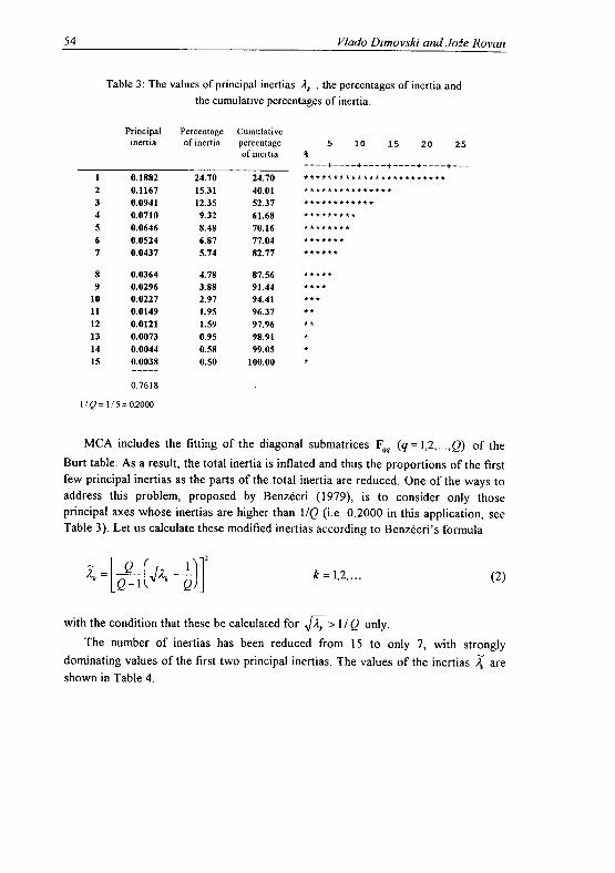
Table 3 : The values of principal inertias Ak , the percentages of inertia andthe cumulative percentages of inertia .

Principal

Percentage Cumulativeinertia

of inertia

percentage

5

10

15

20

25of inertia

%

1

0.1882

24.70

24.702

0.1167

15.31

40.013

0.0941

12.35

52.374

0.0710

9.32

61.685

0.0646

8.48

70.166

0.0524

6.87

77.047

0.0437

5.74

82.77

8

0.0364

4.78

87.569

0.0296

3.88

91.4410

0.0227

2.97

94.4111

0.0149

1.95

96.3712

0.0121

1.59

97.9613

0.0073

0.95

98.9114

0.0044

0.58

99.0515

0.0038

0.50

100.00

0.7618

I / Q = 1/ 5 = 02000

MCA includes the fitting of the diagonal submatrices F99 (q = 1,2, . . .,Q) of theBurt table . As a result, the total inertia is inflated and thus the proportions of the firstfew principal inertias as the parts of the total inertia are reduced . One of the ways toaddress this problem, proposed by Benzécri (1979), is to consider only thoseprincipal axes whose inertias are higher than 1/Q (i .e . 0 .2000 in this application, seeTable 3). Let us calculate these modified inertias according to Benzécri's formula

ik =[Q1(-J1XI

Q

2

++++++++++++++++++++++++

++++++++++++

k =1,2, . . .

(2)

with the condition that these be calculated for FA, > 1 / Q only .The number of inertias has been reduced from 15 to only 7, with strongly

dominating values of the first two principal inertias . The values of the inertias .1 areshown in Table 4 .


55

Table 4 : The values of modified inertias ~ , the respective percentages of inertia and thecumulative percentages of inertia .

Principal

Percentage Cumulativeinertia

of inertia

percentage

10

20

30

40 %of inertia

1

0.085411

44.22

42.222

0.031310

15.48

57.70

3

0.017804

8.80

66.504

0.006888

3.41

69.905

0.004589

2.27

72.176

0.001301

0.64

72.82

7

0.000128

0.06

72.88

j' = 0 .202250

The next question is the quality of the presentation of the position of the profilesbased on a few first principal coordinates . M. Greenacre (1994, pp . 155) calculatesthe percentage of inertia as follows

Ak%=100AZ

k=1,2, . . .

G • = Y•D x

*********************

***

where 02 is an average of the off diagonal inertias X99., i .e .

z -1

Q Q Z

Q

J-Q1

Q(Q - 1)

0

'Q=Q-1

' Q2

v'=v

(3)

(4)

The values of percentages of inertia and the cumulative percentages of inertia arealso shown in Table 4 . According to the above mentioned Greenacre's refinement ofthe MCA solution (3), 57.70% of the total inertia is explained by the first twoprincipal axes . It seems that the representation of the positions of the profiles basedon the first two principal coordinates can serve as a good basis for the analysis of ourexample.

We have already calculated the matrix Y of standard coordinates . Next, we need

to transform the first 7 columns of Y , denoted by Y' into principal coordinates usingthe modified inertias given by formula (2)

(3)

where D. is the diagonal matrix of the 7 modified inertias. The matrix G* is given in

Table 5 .

5 6


Table 5 : The matrix of principal coordinates G * .

1.PC

2.PC

3.PC

4.PC

5.PC

6.PC

7.PC

I

A2

-0.4382

0.3614

-0.2060

0.1313

0.0872

-0.0116

-0.00732

A3

-0.3108

-0.0195

0.1204

-0.0015

-0.0389

0.0471

0.00203

A4

0.1288

-0.0891

-0.0389

-0.0618

-0.0157

-0.0355

-0.00014

A5

0.4314

0.0004

0.1978

0.1118

0.0291

0.0853

0.00505

BI

-0.8357

0.2184

-0.1813

-0.0632

0.4382

0.1622

-0.01626

B2

-0.2863

0.0687

-0.0574

-0.0181

-0.1185

0.0173

0.01127

B3

0.0352

-0.1064

-0.0183

0.0385

0.0396

-0.0418

0.00448

B4

0.4250

0.1181

0.1452

-0.0541

-0.0117

0.0460

-0.02169

C2

-0.3075

-0.0528

0.2006

-0.1239

-0.0098

-0.0216

-0.000710

C3

-0.0059

-0.1151

0.0389

0.1901

0.0060

0.0261

0.004311

C4

0.1267

0.0004

-0.2530

-0.0473

-0.0067

0.0022

-0.002912

C5

0.6933

0.6978

0.2247

-0.0474

0.0483

-0.0296

-0.001113

D2

-0.3401

0.0187

0.1782

-0.0085

-0.0085

-0.0094

-0.005914

D3

0.2975

-0.2572

-0.0023

0.0659

0.0559

-0.0060

0.017215

1)4

0.0897

0.0155

-0.2315

-0.0485

-0.0582

0.0359

-0.009716

D5

0.5285

0.8763

0.0367

0.0315

0.1241

-0.0998

0.017017

E2

-0.4418

0.1639

-0.0350

0.1996

-0.1179

-0.0470

-0.016818

E3

-0.3222

-0.0416

-0.0368

-0.0925

0.1022

0.0075

0.010419

E4

0.3203

-0.1251

0.0354

0.0061

0.0093

-0.0049

-0.013620

E5

0.2156

0.2739

0.0113

-0.0412

-0.1122

0.0496

0.0362

The position of the projections of profilepoints in the optimal subspace of chosendimensionality is defined by the principal coordinates .

The next question that should be answered is whether the position of anindividual profile is well represented in the optimal subspace . The first 7 dimensionsdetermine the modified full space, so we need to calculate how much of therepresentation of the position of an individual profile is accounted for by the firstprincipal coordinate, the first two principal coordinates, the first three principalcoordinates, etc. For that reason, we need to calculate the matrix of cumulativeproportions of inertias of profiles as part of the total inertias of profiles (Rovan,1991). For our investigation this matrix is shown in Table 6 .


57

Table 6 : The matrix of cumulative proportions of inertias of profiles as part of the totalinertias of profiles .

I .PC

2.PC

3.PC

4.PC

5-PC

6.PC

7.PC

I

A2

0.4923

0.8271

0.9359

0.9800

0.9995

0.9999

1 .00002

A3

0.8384

0.8417

0.9676

0.9676

0.9807

1 .0000

1 .00003

A4

0.5290

0.7821

0.8303

0.9519

0.9597

1 .0000

1 .00004

A5

0.7570

0.7570

0.9161

0.9669

0.9703

0.9999

1 .00005

131

0.6974

0.7450

0.7778

0.7818

0.9735

0.9997

1 .00006

B2

0.7824

0.8274

0.8589

0.8620

0.9960

0.9988

1 .00007

B3

0.0700

0.7092

0.7282

0.8120

0.9004

0.9989

1 .00008

B4

0.8162

0.8792

0.9745

0.9877

0.9884

0.9979

1.00009

C2

0.6161

0.6343

0.8964

0.9963

0.9970

1.0000

1 .000010

C3

0.0007

0.2569

0.2863

0.9858

0.9865

0.9996

1.0000II

C4

0.1951

0.1951

0.9721

0.9993

0.9998

0.9999

1.000012

C5

0.4696

0.9454

0.9947

0.9969

0.9991

1.0000

1.000013

D2

0.7812

0.7836

0.9982

0.9987

0.9992

0.9998

1.000014

D3

0.5448

0.9520

0.9520

0.9787

0.9979

0.9982

1.000015

D4

0.1166

0.1200

0.8967

0.9308

0.9799

0.9986

1.000016

D5

0.2598

0.9740

0.9752

0.9762

0.9905

0.9997

1.000017

E2

0.6984

0.7945

0.7989

0.9414

0.9911

0.9990

1.000018

E3

0.8235

0.8373

0.8480

0.9159

0.9987

0.9991

1.000019

E4

0.8563

0.9868

0.9972

0.9975

0.9983

0.9985

1.000020

E5

0.3328

0.8698

0.8708

0.8829

0.9730

0.9906

1.0000Total

7 Map and analysis

The representation of the profiles based on their first two principal coordinates isshown in Figure 1 .

When the proportion of inertia of the first two dimensions as part of the totalinertia is relatively high, then most of the profiles are well represented in a two-dimensional map (by their projections onto a plane) . The two-dimensional solution ofour example explaining 57 .70% of the total inertia can serve as a good basis for thedisplay of the profiles .

However, this general conclusion is not valid for every profile . For completeanalysis every single profile should be well represented which gives the reason forsome profiles to be represented by a higher number of principal coordinates (Rovan,1994) . The cumulative proportions of inertias of the profiles as the parts of the totalinertias of profiles, given in Table 7, are the basis for the conclusion, whether someprofiles are well represented in a two-dimensional map . In our investigation 17 out of20 profiles have cumulative proportions of inertias above 0 .75 and we believe theyare well represented in a two-dimensional map . This is not the case for profiles C3,C4,and D4 that load on higher dimensions .

0 .5793

0.7917

0.9125

0.9592

0.9903

0.9991

1 .0000

5 8

Vlado Dimovski and .Joie Rovan

1.0

0.8

0.6 /

AX

0.4

A2IS

810.2

~ ~

E2

~2

82

B4

D: .

A50.0

=s_~

A`4

-02

i3

-0.4

D5

-1.0

-0.8

-0.6

-0:4

-0.2

0.0

0.2

0.4

0.6

0.8

Axis 1

Figure 1 : Two-dimensional map (data from Table 5) .

In the analysis of a set of ordinal variables it is meaningful to connect thesuccessive category points of each ordinal variable. An approximately parallel patternof the two lines belonging to two ordinal variables reveals a close relationshipbetween these two variables .

The position of the profilepoints can lead to the following conclusions :

• The map shows a strong bi-polarization, with most of the profile pointsrepresenting categories with low environmental turbulence on one side andwith high environmental turbulence on the other side . Therefore, the first axiswith the prevailing proportion of the total inertia represents the direction oflow-to-high environmental turbulence .

• The majority of the connecting lines on the map is parallel to the first principalaxis . This pattern supports our initial hypothesis of having strong relationshipsamong the variables of environmental turbulence . This result also implies thatmost of the variables measure the degree of environmental turbulence .


59

8 Conclusion

Environmental turbulence has been conceptualised as "more events per unit time" . Toverify the developed operationalised construct of environmental turbulence, MCA hasbeen used .

We have investigated the population of credit unions in Ohio . The construct ofenvironmental turbulence has been operationalised by five ordinal scale variables .

Using MCA the original five-dimensional variable space has been reduced intotwo-dimensional subspace explaining about 57.70% of the total variance.

Two-dimensional map of the profilepoints have shown strong bipolarization withmost of the profilepoints representing categories with low environmental turbulenceon one side and with high environmental turbulence on the other side . Therefore, thefirst axis with the prevailing proportion of the total inertia represents the direction oflow-to-high environmental turbulence .

MCA has confirmed our initial hypothesis of having strong relationships amongthe variables of environmental turbulence . This result also implies that most of thevariables measure the degree of environmental turbulence .

References

[1] Benzécri, J .-P . (1979) : Sur le calcul des taux d'inertie dans l'analyse d'unquestionnaire. Addendum et erratum a [BIN.MULT] . Cahiers de L 'analyse desDonnées, 4, 377-378 .

[2] Cool, K . and Schendel, D .E . (1988) : Performance differences among strategic groupmembers . Strategic Management Journal, 9, 207 - 223 .

[3] Day, G . (1977) : Diagnosing the product portfolio . Journal of Marketing, 41, 230-245 .[4] Dess, G .G . and Beard, D .W . (1984): Dimensions of organisational task environments .

Administrative Science Quarterly, 29, 52-73 .[5] Dimovski, V. (1994) : Organisational Learning and Competitive Advantage : A

Theoretical and Empirical Analysis . Unpublished doctoral dissertation, ClevelandState University, USA .

[6] Fiol, C.M. and Lyles, M .A . (1985) : Organisational learning . Academy of ManagementReview, 10, 803-813 .

[7] Glazer, R . (1990) : Marketing in an information-intensive environment : Strategicimplications of knowledge as an asset . Journal of Marketing, 55, 1-19 .

[8] Greenacre, M .J . (1994) : Multiple and joint correspondence analysis . In M .J .Greenacre and J . Blasius (Eds .) ; Correspondence Analysis in the SocialSciences. London : Academic Press, 141-161 .

[9] Miles, R.E ., Snow, C.C ., and Pfeffer, J . (1974) : Organisation-environment : Conceptsand issues . Industrial Relations, 13, 244-264 .

60

Vlado Dimovski and Joze Rovan

[10] Reichert, A .K . and Rubens, J . (1994) : Risk management techniques employed withinthe U .S . credit union industry . Journal of Business Finance and Accounting, 21, 15-35 .

[11] Reimann, B .C . (1987) : Managing for Value. Oxford. Basil Blackwell .[12] Rovan, J . (1991) : The role of the Andrews' curves in correspondence analysis . In

Proceedings of the SAS European Users Group International Conference . SASInstitute, 460-474 .

[13] Rovan, J .(1994) : Visualizing solutions in more than two dimensions . In M . Greenacreand J. Blasius (Eds .) : Correspondence Analysis in the Social Sciences, London :Academic Press, 210-229 .

[14] Thompson, J .D . (1967) : Organisations inaction . New York: McGraw-Hill .

[15] Tung, R .L . (1979) : Dimensions of organisational environment : An exploratorystudy of their impact on organisation structure_ Academy of ManagementJournal, 22, 672-693 .

[16] Wortman, M.S . (1979) . Strategic management : Not-for-profit organizations . InD.E. Schendel and C.W. Hofer (Eds .) : Strategic Management : A New View ofBusiness Policy and Planing, Boston: Little, Brown and Company, 353-381 .

environmental turbulence in the credit union...

Documents