environmental policy integrated climate...

Environmental

Policy Integrated

Climate Model

User’s Manual Version 0810

September 2015

v

EPIC - ENVIRONMENTAL POLICY INTEGRATED CLIMATE

EPIC Development Team:

Dr. Tom Gerik Co-project leader, quality control and beta testing

Dr. Jimmy Williams† Author of EPIC

Steve Dagitz Visual Basic programming Melanie Magre Database maintenance, beta testing, guide development Avery Meinardus EPIC programming support Evelyn Steglich Model validation, website maintenance, guide development Robin Taylor EPIC 0810 User Manual revision

Blackland Research and Extension Center Texas A&M AgriLife

720 East Blackland Road Temple, Texas

iv

Disclaimer

Warning: copyright law and international treaties protect this computer program. Unauthorized reproduction or distribution of this program, or any portion of it, may result in severe civil and criminal penalties and will be prosecuted to the full extent of the law.

Information presented is based upon best estimates available at the time prepared. The Texas A&M University System makes no warranty, expressed or implied, or assumes any legal liability or responsibility for the accuracy, completeness or usefulness of any

information.

iii

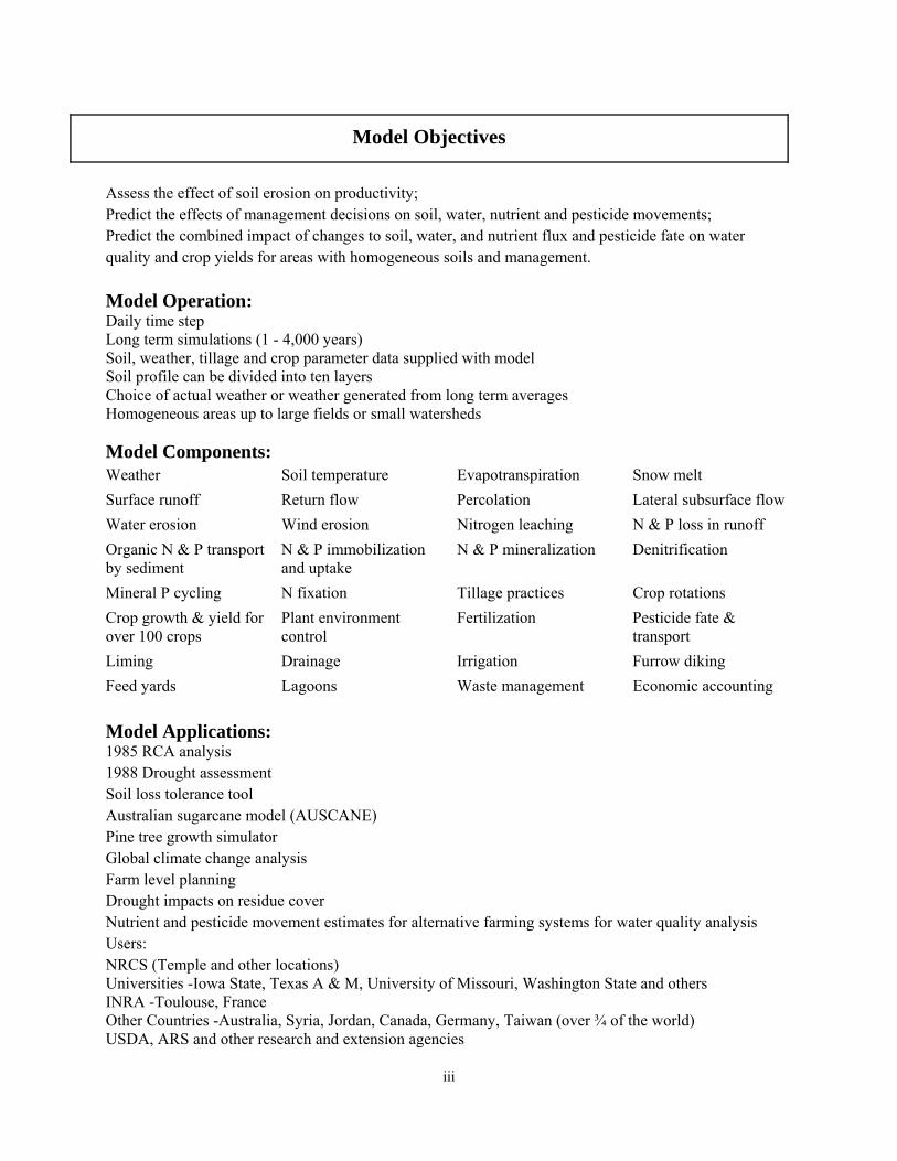
Model Objectives

Assess the effect of soil erosion on productivity; Predict the effects of management decisions on soil, water, nutrient and pesticide movements; Predict the combined impact of changes to soil, water, and nutrient flux and pesticide fate on water quality and crop yields for areas with homogeneous soils and management.

Model Operation: Daily time step Long term simulations (1 - 4,000 years) Soil, weather, tillage and crop parameter data supplied with model Soil profile can be divided into ten layers Choice of actual weather or weather generated from long term averages Homogeneous areas up to large fields or small watersheds

Model Components: Weather Soil temperature Evapotranspiration Snow melt

Surface runoff Return flow Percolation Lateral subsurface flow

Water erosion Wind erosion Nitrogen leaching N & P loss in runoff

Organic N & P transport by sediment

N & P immobilization and uptake

N & P mineralization Denitrification

Mineral P cycling N fixation Tillage practices Crop rotations

Crop growth & yield for over 100 crops

Plant environment control

Fertilization Pesticide fate & transport

Liming Drainage Irrigation Furrow diking

Feed yards Lagoons Waste management Economic accounting

Model Applications: 1985 RCA analysis 1988 Drought assessment Soil loss tolerance tool Australian sugarcane model (AUSCANE) Pine tree growth simulator Global climate change analysis Farm level planning Drought impacts on residue cover Nutrient and pesticide movement estimates for alternative farming systems for water quality analysis Users: NRCS (Temple and other locations) Universities -Iowa State, Texas A & M, University of Missouri, Washington State and others INRA -Toulouse, France Other Countries -Australia, Syria, Jordan, Canada, Germany, Taiwan (over ¾ of the world) USDA, ARS and other research and extension agencies

ii

Executive Summary

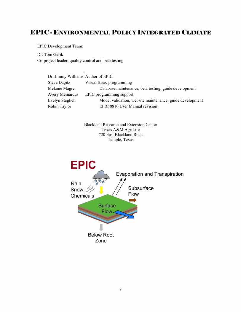
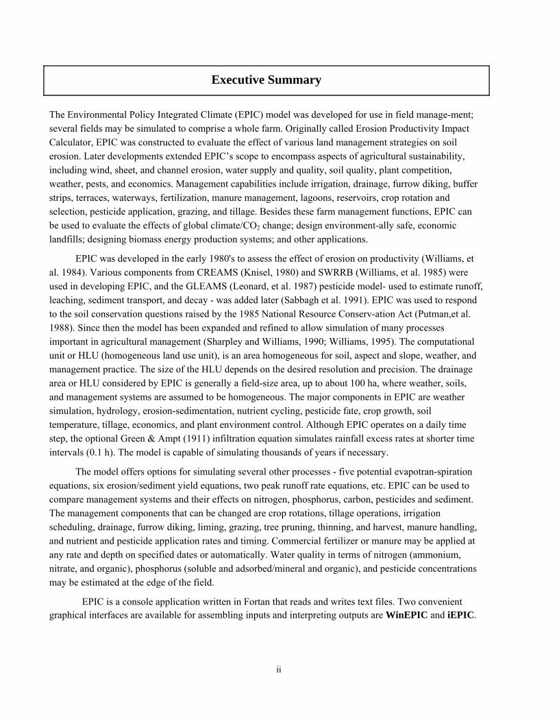
The Environmental Policy Integrated Climate (EPIC) model was developed for use in field manage-ment; several fields may be simulated to comprise a whole farm. Originally called Erosion Productivity Impact Calculator, EPIC was constructed to evaluate the effect of various land management strategies on soil erosion. Later developments extended EPIC’s scope to encompass aspects of agricultural sustainability, including wind, sheet, and channel erosion, water supply and quality, soil quality, plant competition, weather, pests, and economics. Management capabilities include irrigation, drainage, furrow diking, buffer strips, terraces, waterways, fertilization, manure management, lagoons, reservoirs, crop rotation and selection, pesticide application, grazing, and tillage. Besides these farm management functions, EPIC can be used to evaluate the effects of global climate/CO2 change; design environment-ally safe, economic landfills; designing biomass energy production systems; and other applications.

EPIC was developed in the early 1980's to assess the effect of erosion on productivity (Williams, et al. 1984). Various components from CREAMS (Knisel, 1980) and SWRRB (Williams, et al. 1985) were used in developing EPIC, and the GLEAMS (Leonard, et al. 1987) pesticide model- used to estimate runoff, leaching, sediment transport, and decay - was added later (Sabbagh et al. 1991). EPIC was used to respond to the soil conservation questions raised by the 1985 National Resource Conserv-ation Act (Putman,et al. 1988). Since then the model has been expanded and refined to allow simulation of many processes important in agricultural management (Sharpley and Williams, 1990; Williams, 1995). The computational unit or HLU (homogeneous land use unit), is an area homogeneous for soil, aspect and slope, weather, and management practice. The size of the HLU depends on the desired resolution and precision. The drainage area or HLU considered by EPIC is generally a field-size area, up to about 100 ha, where weather, soils, and management systems are assumed to be homogeneous. The major components in EPIC are weather simulation, hydrology, erosion-sedimentation, nutrient cycling, pesticide fate, crop growth, soil temperature, tillage, economics, and plant environment control. Although EPIC operates on a daily time step, the optional Green & Ampt (1911) infiltration equation simulates rainfall excess rates at shorter time intervals (0.1 h). The model is capable of simulating thousands of years if necessary.

The model offers options for simulating several other processes - five potential evapotran-spiration equations, six erosion/sediment yield equations, two peak runoff rate equations, etc. EPIC can be used to compare management systems and their effects on nitrogen, phosphorus, carbon, pesticides and sediment. The management components that can be changed are crop rotations, tillage operations, irrigation scheduling, drainage, furrow diking, liming, grazing, tree pruning, thinning, and harvest, manure handling, and nutrient and pesticide application rates and timing. Commercial fertilizer or manure may be applied at any rate and depth on specified dates or automatically. Water quality in terms of nitrogen (ammonium, nitrate, and organic), phosphorus (soluble and adsorbed/mineral and organic), and pesticide concentrations may be estimated at the edge of the field.

EPIC is a console application written in Fortan that reads and writes text files. Two convenient graphical interfaces are available for assembling inputs and interpreting outputs are WinEPIC and iEPIC.

i

Contents

EPIC Development Team ........................................................................................................................ iv Discalimer ................................................................................................................................................ iv Model Objectives ..................................................................................................................................... iii Executive Summary .................................................................................................................................. ii Contents ..................................................................................................................................................... i

Overview ................................................................................................................................................... 1 EPIC Data Structure .................................................................................................................................. 7 Master File (EPICFILE.dat) ..................................................................................................................... 9 Run File (EPICRUN.dat) ........................................................................................................................ 14 Control File (EPICCONT.dat) ................................................................................................................ 15 Site File (SITE0810.dat & filename.sit) .................................................................................................. 21 Soil Files (SOIL0810.dat & filename.sol) ............................................................................................... 23 Weather Files (WPM10810.dat & filename.wpl) .................................................................................... 26 Wind Files (WIND0810.dat & filename.wnd) ......................................................................................... 29 How to Prepare Weather Input Files ....................................................................................................... 31 Operation Schedule Files (OPSC0810.dat & filename.ops) ................................................................... 33 Crop File (CROP0810.dat) ..................................................................................................................... 39 Tillage File (TILL0810.dat) .................................................................................................................... 46 Fertilizer File (FERT0810.dat) ............................................................................................................... 49 Pesticide File (PEST0810.dat) ................................................................................................................ 50 Multi-Run File (MLRN0810.dat) ............................................................................................................ 51 Parameter File (PARM0810.dat) ............................................................................................................. 52 Print File (PRNT0810.dat) ...................................................................................................................... 59 Output Analyzer ...................................................................................................................................... 78 How to Validate Crop Yields .................................................................................................................. 82 How to Validate Runoff, Sediment Losses & Sediment Losses ............................................................. 84 Pesticide Fate – The GLEAMS Model ................................................................................................... 88 References ............................................................................................................................................... 91

1

Overview

EPIC is a process-based computer model that simulates the physico-chemical processes that occur in soil and water under agricultural management. It is designed to simulate a field, farm or small watershed that is homogenous with respect to climate, soil, land use, and topography – termed a hydrologic land use unit (HLU). The area modeled may be of any size consistent with required HLU resolution. EPIC operates solely in time; there is no explicitly spatial component. Output from the model includes files giving the water, nutrient, and pesticide flux in the HLU at time scales from daily to annual. The growth of crop plants is simulated depending on the availability of nutrients and water and subject to ambient temperature and sunlight. The crop and land management methods used by growers can be simulated in considerable detail.

The model can be subdivided into nine separate components defined as weather, hydrology, erosion, nutrients, soil temperature, plant growth, plant environment control, tillage, and economic budgets (Williams 1990). It is a field-scale model that is designed to simulate drainage areas that are characterized by homogeneous weather, soil, landscape, crop rotation, and management system parameters. It operates on a continuous basis using a daily time step and can perform long-term simulations for hundreds and even thousands of years. A wide range of crop rotations and other vegetative systems can be simulated with the generic crop growth routine used in EPIC. An extensive array of tillage systems and other management practices can also be simulated with the model. Seven options are provided to simulate water erosion and five options are available to simulate potential evapotranspiration (PET). Detailed discussions of the EPIC components and functions are given in Williams et al. (1984), Williams (1990), Sharply & Williams (1990), and Williams (1995).

Brief History of EPIC

The original function of EPIC was to estimate soil erosion by water under different crop and land management practices, a function reflected its original name: Erosion Productivity Impact Calculator. The development of the field-scale EPIC model was initiated in 1981 to support assessments of soil erosion impact on soil productivity for soil, climate, and cropping practices representative on a broad spectrum of U.S. agricultural production regions. The first major application of EPIC was a national analysis performed in support of the 1985 Resources Conservation Act (RCA) assessment. The model has continuously evolved since that time and has been used in a wide range of field, regional, and national studies both in the U.S. and in other countries. The range of EPIC applications has also expanded greatly over that time including studies of:

Irrigation;

Climate change effects on crop yields;

Nutrient cycling and nutrient loss;

Wind and water erosion;

Soil carbon sequestration;

Economic and environmental;

2

Comprehensive regional assessments.

Modeling pesticide fate

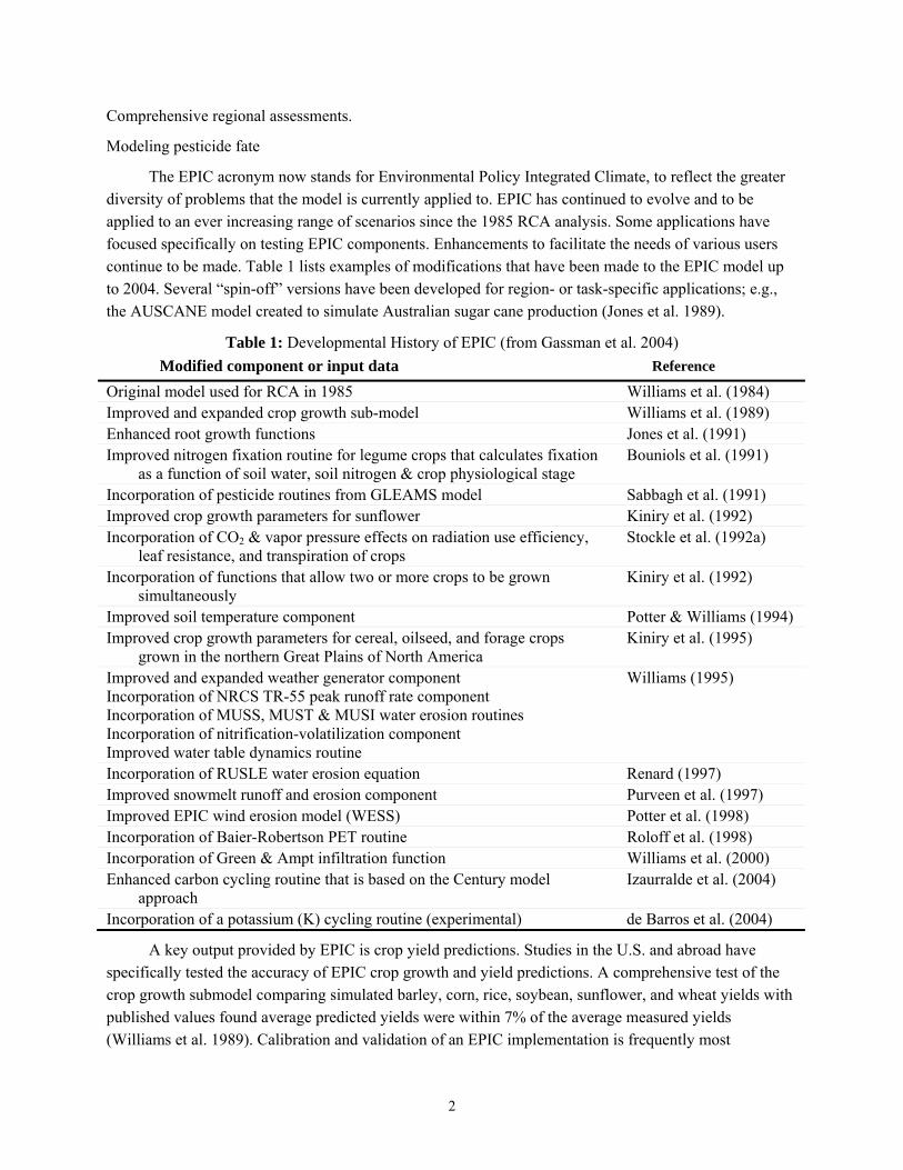
The EPIC acronym now stands for Environmental Policy Integrated Climate, to reflect the greater diversity of problems that the model is currently applied to. EPIC has continued to evolve and to be applied to an ever increasing range of scenarios since the 1985 RCA analysis. Some applications have focused specifically on testing EPIC components. Enhancements to facilitate the needs of various users continue to be made. Table 1 lists examples of modifications that have been made to the EPIC model up to 2004. Several “spin-off” versions have been developed for region- or task-specific applications; e.g., the AUSCANE model created to simulate Australian sugar cane production (Jones et al. 1989).

Table 1: Developmental History of EPIC (from Gassman et al. 2004)

Modified component or input data Reference

Original model used for RCA in 1985 Williams et al. (1984) Improved and expanded crop growth sub-model Williams et al. (1989) Enhanced root growth functions Jones et al. (1991) Improved nitrogen fixation routine for legume crops that calculates fixation

as a function of soil water, soil nitrogen & crop physiological stage Bouniols et al. (1991)

Incorporation of pesticide routines from GLEAMS model Sabbagh et al. (1991) Improved crop growth parameters for sunflower Kiniry et al. (1992) Incorporation of CO2 & vapor pressure effects on radiation use efficiency,

leaf resistance, and transpiration of crops Stockle et al. (1992a)

Incorporation of functions that allow two or more crops to be grown simultaneously

Kiniry et al. (1992)

Improved soil temperature component Potter & Williams (1994) Improved crop growth parameters for cereal, oilseed, and forage crops

grown in the northern Great Plains of North America Kiniry et al. (1995)

Improved and expanded weather generator component Incorporation of NRCS TR-55 peak runoff rate component Incorporation of MUSS, MUST & MUSI water erosion routines Incorporation of nitrification-volatilization component Improved water table dynamics routine

Williams (1995)

Incorporation of RUSLE water erosion equation Renard (1997) Improved snowmelt runoff and erosion component Purveen et al. (1997) Improved EPIC wind erosion model (WESS) Potter et al. (1998) Incorporation of Baier-Robertson PET routine Roloff et al. (1998) Incorporation of Green & Ampt infiltration function Williams et al. (2000) Enhanced carbon cycling routine that is based on the Century model

approach Izaurralde et al. (2004)

Incorporation of a potassium (K) cycling routine (experimental) de Barros et al. (2004)

A key output provided by EPIC is crop yield predictions. Studies in the U.S. and abroad have specifically tested the accuracy of EPIC crop growth and yield predictions. A comprehensive test of the crop growth submodel comparing simulated barley, corn, rice, soybean, sunflower, and wheat yields with published values found average predicted yields were within 7% of the average measured yields (Williams et al. 1989). Calibration and validation of an EPIC implementation is frequently most

3

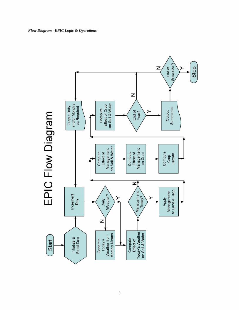
Flow Diagram –EPIC Logic & Operations

4

conveniently accomplished using published crop yield data.

Definitions: EPIC Projects, Scenarios & Runs

A project is a study designed to model and explore an idea or concept regarding the impact of agricultural management practice(s), geography (location and/or topography), or climate on crop yield, environmental impact, and/or economics of the agricultural enterprise. It will involve the manipulation of one or more variables (e.g. presence or absence of a management practice or constant versus increasing atmospheric CO2). Each model execution with a defined set of input data is a scenario. A scenario may be run standalone or as a member of a batch run. A scenario is therefore a single specific model configuration within a project or study which will typically consist of one or more runs of one or more scenarios. The following examples illustrate the flexibility of EPIC to simulate the environmental impact of agriculture:

An EPIC project may involve the same crop and land management scenario applied to several separate parcels of land (a field, farm, or small watershed), each with different soil and/or weather input in a series

of runs;

An EPIC project may involve a variety of management scenarios applied in a series of runs to the same

parcel of land having the same soil and weather files;

An EPIC project may be created for a virtual or real parcel of land subjected to the same scenario (management practices, soil, and weather kept constant), while the geographic characteristics (latitude,

longitude, altitude, slope, or aspect) of the site are varied in a series of runs.

EPIC Applications

Irrigation studies

Yield estimates by EPIC simulations of irrigation experiments in California, Minnesota, Oklahoma, Texas, Virginia, Ontario, and Quebec agreed well with the observed yields of a wide range of crops (reviewed in Gassman et al. 2004).

Climate change effects on crop yields

EPIC simulates the effects of changes in CO2 concentrations and vapor pressure deficit on crop growth and yield via radiation-use efficiency, leaf resistance, and transpiration. Assessments of potential CO2 and climate change impacts on crop yields of corn, wheat, and soybean cropping systems in the central U.S predicted increases in yield in response to increased CO2 and variable changes in yield in response to changing temperature and precipitation (Stockle et al. 1992a,b). The impact of tropical Pacific El Niño Southern Oscillation (ENSO) phenomena on crop yields has been assessed using EPIC (Izaurralde et al. 1999, Legler et al. 1999, Adams et al. 2003) and the effect of sea surface temperature anomalies (SSTA) on potato fertilization management has been investigated in Chile (Meza & Wilks 2004).

5

Nutrient cycling and nutrient loss studies

Validation studies show that EPIC satisfactorily simulates measured soil nitrogen (N) and/or crop N uptake levels and leached N below the root zone or in tile flow are generally accurately predicted (See Tables 2 & 3 in Gassman et al. 2004). Sensitivity analyses shows that EPIC N leaching estimates can be very sensitive to choice of evapotranspiration routine, soil moisture estimates, curve number, precipitation, solar radiation, and soil bulk density (Roloff et al. 1998c, Benson et al. 1992).

Wind and water erosion studies

Several water erosion models are implemented in EPIC: Universal Soil Loss Equation (USLE); Onstad-Foster (AOF) version of USLE ; Modified USLE (MUSLE & RUSLE); and three MUSLE variants, MUST, MUSS & MUSI. These models differ primarily in how the energy component is modeled (Williams et al. 1983, 1984, Williams 1995). The wind erosion model is the Wind Erosion Stochastic Simulator (WESS; Potter et al. 1998). Numerous EPIC applications have been performed for soil erosion (see Gassman et al. [2004] for example applications including validation and scenario studies).

Soil carbon sequestration

Based on concepts used in the Century model (Parton et al. 1994), EPIC simulates carbon and nitrogen compounds stored in and converted between biomass, slow, and passive soil pools. Carbon leaching from surface litter to deeper soil layers and the effect of soil texture on organic matter stabilization are also modeled. Simulations of sites in Nebraska, Kansas, Texas, and Alberta showed EPIC satisfactorily replicated the soil carbon dynamics over a range of environmental conditions and cropping/vegetation and management systems (Izaurralde et al. 2004). EPIC performed robustly for simulations of deforested conditions, cropping systems, and native vegetation in Argentina (Apezteguía et al. 2002). Soil organic carbon (SOC) values estimated in an EPIC simulation of a conservation tillage compared favorably with measured SOC rates (Zhao et al. 2004).

Economic and environmental studies

EPIC tracks production costs and crop income for input to economic models. The FLIPSIM whole farm economic model has been coupled with EPIC to perform economic analyses of irrigated agriculture in Texas (Ellis et al. 1993, Gray et al. 1997). Other examples of economic analyses using EPIC are given in Table 4 of Gassman et al. (2004).

Comprehensive regional assessments

EPIC has been used in a number of studies to evaluate the impacts of cropping systems, management practices, and environmental conditions on multiple environmental indicators. Studies have focused on evaluating specific agricultural policy options, including those conducted by the USDA Natural Resources Conservation Service (NRCS). The first application of EPIC by the NRCS was to evaluate the potential loss in cropland productivity into the future for the 2nd Resources Conservation Act evaluation. Other examples of Comprehensive regional assessments using EPIC are given in Table 5 of Gassman et al. (2004).

6

Modeling pesticide fate

Leonard et al.’s (1987) GLEAMS pesticide fate model is incorporated into EPIC (Sabbagh et al. 1991); it has been tested for pesticide movement and losses by Williams et al. (1992) and Sabbagh et al. (1992), and used to estimate the impact of atrazine loss on water quality (Harman et al. 2004).

7

EPIC Data Structure

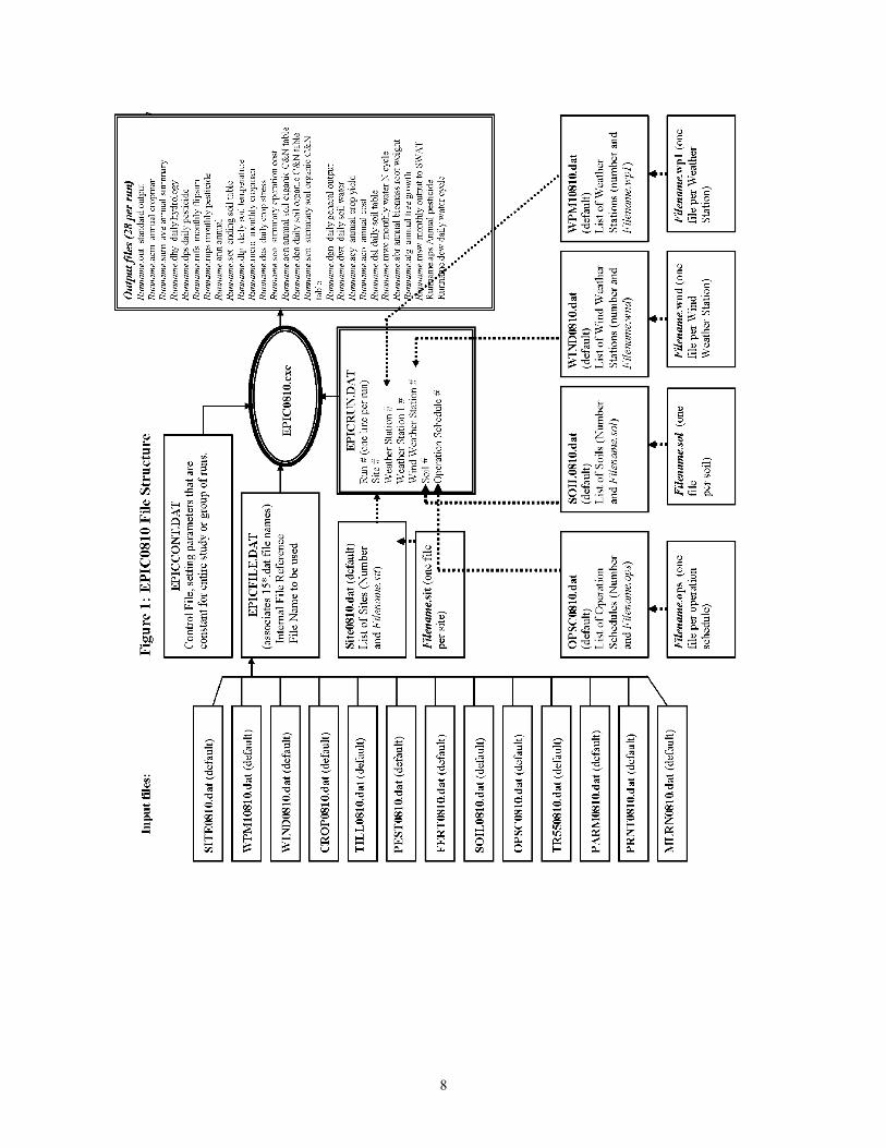
For a given study, a Run Definition file specifies which site, soil, weather, and schedule files are to be used for each scenario in a run. For a given study, the major data elements to be developed by a user include descriptions of sites, soils, field operation schedules, weather, and the constant data. An overview of the files and data flow is given in Figure 1 and the file structure and linkage are briefly discussed below.

9

Master File (EPICFILE.dat)

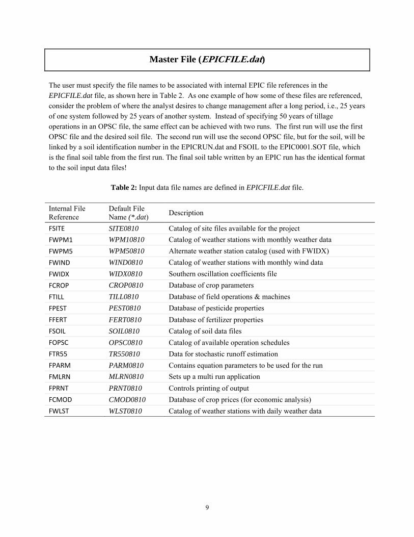
The user must specify the file names to be associated with internal EPIC file references in the EPICFILE.dat file, as shown here in Table 2. As one example of how some of these files are referenced, consider the problem of where the analyst desires to change management after a long period, i.e., 25 years of one system followed by 25 years of another system. Instead of specifying 50 years of tillage operations in an OPSC file, the same effect can be achieved with two runs. The first run will use the first OPSC file and the desired soil file. The second run will use the second OPSC file, but for the soil, will be linked by a soil identification number in the EPICRUN.dat and FSOIL to the EPIC0001.SOT file, which is the final soil table from the first run. The final soil table written by an EPIC run has the identical format

to the soil input data files!

Table 2: Input data file names are defined in EPICFILE.dat file.

Internal File Reference

Default File Name (*.dat)

Description

FSITE SITE0810 Catalog of site files available for the project

FWPM1 WPM10810 Catalog of weather stations with monthly weather data

FWPM5 WPM50810 Alternate weather station catalog (used with FWIDX)

FWIND WIND0810 Catalog of weather stations with monthly wind data

FWIDX WIDX0810 Southern oscillation coefficients file

FCROP CROP0810 Database of crop parameters

FTILL TILL0810 Database of field operations & machines

FPEST PEST0810 Database of pesticide properties

FFERT FERT0810 Database of fertilizer properties

FSOIL SOIL0810 Catalog of soil data files

FOPSC OPSC0810 Catalog of available operation schedules

FTR55 TR550810 Data for stochastic runoff estimation

FPARM PARM0810 Contains equation parameters to be used for the run

FMLRN MLRN0810 Sets up a multi run application

FPRNT PRNT0810 Controls printing of output

FCMOD CMOD0810 Database of crop prices (for economic analysis)

FWLST WLST0810 Catalog of weather stations with daily weather data

10

Execution of Runs. EPIC0810 is a compiled Fortran program. It may be run from the command line or via a dedicated interface, such as WinEPIC or i_EPIC. When run from the command line, the directory

containing the EPIC0810.exe must contain all the input files.

A set of three files controls the flow and scope of an EPIC simulation:

EPICFILE.dat lists the run-specific data files and renames them if required;

EPICCONT.dat controls the run length, various run options and defaults for the project;

EPICRUN.dat lists the site-specific data files and initiates a run of one or more scenarios.

These files may be edited but not renamed; all other files may be renamed with the new names defined in EPICFILE.dat (Table 1).

Files Definition

EPICFILE.dat file provide EPIC with the names of the data files. This file cannot be renamed, but can be edited.

Project Constants

EPICCONT.dat file contains parameters that will be held constant for the entire study, e.g., number of years of simulation, period of simulation, output print specification, weather generator options, etc. This file cannot be renamed, but can be edited.

Runs EPICRUN.dat file includes one row of data for each scenario. Each row of data assigns a unique run number to the scenario and specifies which site, weather station, soil, and tillage operation schedule files will be used. Scenarios are listed one to a line; a run is terminated when a blank line or EOF is reached.

Two weather files may be specified: the weather and wind weather files. If the regular weather and wind station identification parameters are zero, EPIC will use the latitude and longitude data from the filename.sit file and choose the closest weather and wind stations, listed in the WPM1MO.dat and WINDMO.dat files, respectively.

This file cannot be renamed, but can be edited.

Sites EPIC looks in the site catalog file SITE0810.dat (or the catalog named in EPICFILE.dat) for the site number referenced in EPICRUN.dat and obtains the name of the file containing the site-specific data.

The site-specific file is used to describe each Hydrologic Landuse Unit (HLU), which is homogenous with respect to climate, soil, landuse, and topography. The site may be of any size consistent with required HLU resolution. Site files (filename.sit ) describe each site: latitude, longitude, elevation, area, etc. A project may involve several sites (typically fields, but could be a larger area). Sites (fields) may contain buffers and filter strips, etc.

The site catalog SITE0810.dat and the site files can be renamed and edited.

11

Soils EPIC looks in the soil catalog file SOIL0810.dat (or the catalog named in EPICFILE.dat) for the soil number referenced in EPICRUN.dat and obtains the name of the file containing the soil-specific data.

The soil-specific file named filename.sol listed in the catalog file contains data describing the soil profile and the individual horizons. The study may involve several different soils for the farm or watershed analysis and are selected for use in the subarea file.

The soil catalog SOIL0810.dat and the soil files can be renamed and edited.

Weather Weather and wind data files are listed in three catalogs WLST0810.dat, WPM10810.dat & WIND0810.dat for daily weather, monthly climate averages, and average monthly wind roses respectively. EPICRUN.dat defines the run-specific catalog entries to be used. The daily catalog points to files containing daily weather data and the monthly catalogs point to individual files containing long term climate and wind averages (typically 30 years). Databases of averages at U.S. weather stations are included with the program. If no weather or wind file is specified in EPICRUN.dat, EPIC will find the closest station given the latitude and longitude given in SITE08010.da and generate daily weather from the long-term averages in the wind and weather files.

Daily weather data are: solar radiation (mJ/m2 or Langley); maximum and minimum temperatures (°C); precipitation (mm); relative humidity (fraction) or dew point temperature (>1°C); and wind speed averaged over the month (m/s).

Monthly climate data are: mean and standard deviation of maximum air temperature (°C); mean and standard deviation of minimum air temperature (°C); mean (mm), standard deviation (mm), and skewness of precipitation; the probability of wet day after dry day and the probability of a wet day after wet day; number days of rain per month; maximum half hour rainfall (mm); mean solar radiation (MJ/m2 or Langley); mean relative humidity (fraction); and mean wind speed (m/s).

Monthly wind data are: average monthly wind speed (m/s); and % of time the wind is from the 16 cardinal points starting with North (N, NNE, NE, ENE, E, ESE, SE, SSE, S, SSW, SW, WSW, W, WNW, NW, NNW).

WLST0810 EPIC looks in the daily weather file catalog WLST0810.dat for the numbered daily weather station file referenced in EPICRUN.dat.

Daily weather files have the form filename.dly and contain the date and the 6 weather variables listed above.

The weather catalog WLST0810.dat and the weather file can be renamed and edited.

WPM10810 EPIC looks in the monthly weather file catalog WPM10810.dat for the numbered monthly weather station file referenced in EPICRUN.dat.

Monthly weather files have the form filename.wpm and contain the 13 weather variables listed above.

The weather catalog WPM10810.dat and the weather file can be renamed and edited.

WIND0810 EPIC looks in the monthly wind file catalog WIND0810.dat for the numbered monthly wind station file referenced in EPICRUN.dat.

Monthly wind station files have the form filename.wnd and contain monthly average wind run and the 16 cardinal points wind rose.

The wind catalog WIND0810.dat and the wind file can be renamed and edited.

12

WPM50810 EPIC looks in an alternate catalog of monthly weather stations for use with the southern oscillation coefficients in WIDX0810.dat. Monthly weather files have the form filename.wp5 and contain 13 weather variables. filename.wp5 files have the same structure as filename.wpm which may be referenced in WPM50810.dat.

This feature is experimental and should be validated if used.

WIDX0810 EPIC reads a file containing coefficients for adjusting monthly averages according to the phase of the southern oscillation, if this correction is requested.

This feature is experimental and should be validated if used.

Operation Schedules

EPIC looks in the operation schedule catalog file OPSC0810.dat (or the catalog named in EPICFILE.dat) for the operation schedule number referenced in EPICRUN.dat and obtains the name of the file containing the required operation schedule.

The operations file named filename.ops listed in the catalog file contains the schedule of management events for the HLU in the field, farm or small watershed study. It describes the unique landuse operations such as crops and crop rotations with typical tillage operations, ponds or reservoir, farmstead with or without lagoon, etc. for the HLU over a defined period. The events defined in the selected filename.ops are repeated until the simulation terminates after NBYR years. Schedules may be combined to create a new cropping system.

The operations catalog OPSC0810.dat and the operations files can be renamed and edited. New schedules may be added by appending a new record with unique reference number to OPSC0810.dat.

Crops Crops are maintained in a database CROP0810.dat.This file contains data crop characteristics in 56 fields containing parameters describing the crop and its growth characteristics.

The crops database CROP0810.dat can be renamed and edited. New plants may be added by appending a new record with unique reference number to CROP0810.dat.

Tillage Tillage operations are maintained in the database TILL0810.dat. This file includes the operations (e.g. sowing, fertilizing, harvesting, etc.) and the equipment used in the operation. An operation therefore may have several entries, one for each of several pieces of machinery designed to execute the operation (e.g. different kinds of planter, sprayer, or harvester).

The tillage database TILL0810.dat can be renamed and edited. New tillage operations may be added by appending a new record with unique reference number to TILL0810.dat.

Fertilizers Fertilizer properties are maintained in the database FERT0810.dat. The database includes both organic and inorganic nutrient components in 8 fields, plus name and cost. Some commercial fertilizers have potassium in the mix but EPIC does not utilize K20 in the simulated nutrient uptake/yield relationship.

The fertilizer database FERT0810.dat can be renamed and edited. New fertilizers may be added by appending a new record with unique reference number to FERT0810.dat.

Pesticides Pesticide properties are maintained in the database PEST0810.dat. Properties include solubility, half-life, and carbon absorption coefficient. Database includes most common pesticides used in the USA during the past 20 years.

The pesticides database PEST0810.dat can be renamed and edited. New pesticides may be added by appending a new record with unique reference number to PEST0810.dat.

13

Print Includes the control data for printing selected output variables in the sections of the EPIC0810.out file and 19 other summary files.

The print definition file PRNT0810.dat can be renamed and edited.

Parameter Includes numerous model parameters.

The parameter file PARM0810.dat can be renamed but should not be edited without first consulting the developers.

Multi-Run There are circumstances in which a number of runs of the same scenario must be executed; for example, with different generated weather in order to obtain a distribution of soil erosion. This file defines the options for selecting different consecutive weather runs without reloading the inputs.

The multi-run control file MLRN0810.dat can be renamed and edited.

EPIC Version 0810 is a compiled Fortran program with very specific format and file structure

requirements. Description of the input files and definitions of the input variables follows.

14

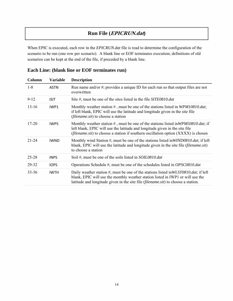
Run File (EPICRUN.dat)

When EPIC is executed, each row in the EPICRUN.dat file is read to determine the configuration of the scenario to be run (one row per scenario). A blank line or EOF terminates execution; definitions of old scenarios can be kept at the end of the file, if preceded by a blank line.

Each Line: (blank line or EOF terminates run)

Column Variable Description

1-8 ASTN Run name and/or #; provides a unique ID for each run so that output files are not overwritten

9-12 ISIT Site #, must be one of the sites listed in the file SITE0810.dat

13-16 IWP1 Monthly weather station # , must be one of the stations listed in WPM10810.dat; if left blank, EPIC will use the latitude and longitude given in the site file (filename.sit) to choose a station

17-20 IWP5 Monthly weather station # , must be one of the stations listed inWPM50810.dat; if left blank, EPIC will use the latitude and longitude given in the site file (filename.sit) to choose a station if southern oscillation option (XXXX) is chosen

21-24 IWND Monthly wind Station #, must be one of the stations listed inWIND0810.dat; if left blank, EPIC will use the latitude and longitude given in the site file (filename.sit) to choose a station

25-28 INPS Soil #, must be one of the soils listed in SOIL0810.dat

29-32 IOPS Operations Schedule #, must be one of the schedules listed in OPSC0810.dat

33-36 IWTH Daily weather station #, must be one of the stations listed inWLST0810.dat; if left blank, EPIC will use the monthly weather station listed in IWP1 or will use the latitude and longitude given in the site file (filename.sit) to choose a station.

15

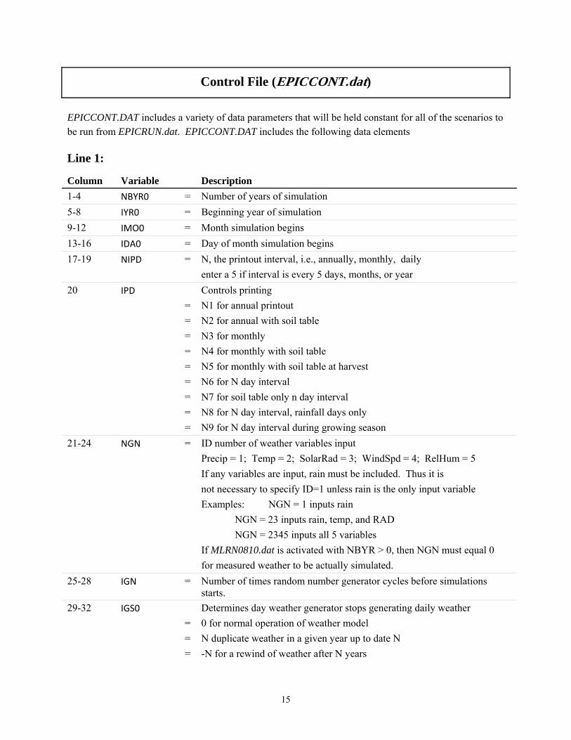
Control File (EPICCONT.dat)

EPICCONT.DAT includes a variety of data parameters that will be held constant for all of the scenarios to be run from EPICRUN.dat. EPICCONT.DAT includes the following data elements

Line 1:


1-4 NBYR0 = Number of years of simulation

5-8 IYR0 = Beginning year of simulation

9-12 IMO0 = Month simulation begins

13-16 IDA0 = Day of month simulation begins

17-19 NIPD = N, the printout interval, i.e., annually, monthly, daily

enter a 5 if interval is every 5 days, months, or year

20 IPD Controls printing

= N1 for annual printout

= N2 for annual with soil table

= N3 for monthly

= N4 for monthly with soil table

= N5 for monthly with soil table at harvest

= N6 for N day interval

= N7 for soil table only n day interval

= N8 for N day interval, rainfall days only

= N9 for N day interval during growing season

21-24 NGN = ID number of weather variables input

Precip = 1; Temp = 2; SolarRad = 3; WindSpd = 4; RelHum = 5

If any variables are input, rain must be included. Thus it is

not necessary to specify ID=1 unless rain is the only input variable

Examples: NGN = 1 inputs rain

NGN = 23 inputs rain, temp, and RAD

NGN = 2345 inputs all 5 variables

If MLRN0810.dat is activated with NBYR > 0, then NGN must equal 0

for measured weather to be actually simulated.

25-28 IGN = Number of times random number generator cycles before simulations starts.

29-32 IGS0 Determines day weather generator stops generating daily weather

= 0 for normal operation of weather model

= N duplicate weather in a given year up to date N

= -N for a rewind of weather after N years

16

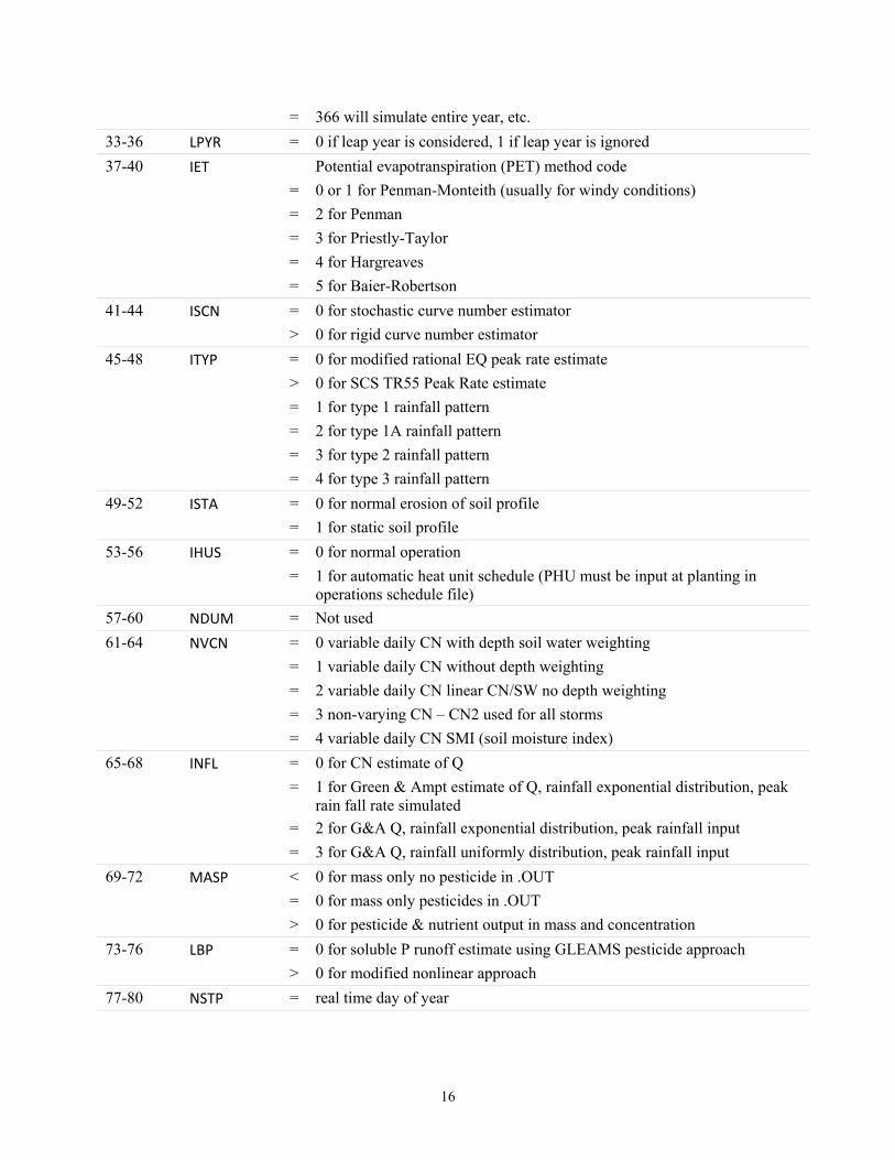
= 366 will simulate entire year, etc.

33-36 LPYR = 0 if leap year is considered, 1 if leap year is ignored

37-40 IET Potential evapotranspiration (PET) method code

= 0 or 1 for Penman-Monteith (usually for windy conditions)

= 2 for Penman

= 3 for Priestly-Taylor

= 4 for Hargreaves

= 5 for Baier-Robertson

41-44 ISCN = 0 for stochastic curve number estimator

> 0 for rigid curve number estimator

45-48 ITYP = 0 for modified rational EQ peak rate estimate

> 0 for SCS TR55 Peak Rate estimate

= 1 for type 1 rainfall pattern

= 2 for type 1A rainfall pattern



49-52 ISTA = 0 for normal erosion of soil profile

= 1 for static soil profile

53-56 IHUS = 0 for normal operation

= 1 for automatic heat unit schedule (PHU must be input at planting in operations schedule file)

57-60 NDUM = Not used

61-64 NVCN = 0 variable daily CN with depth soil water weighting

= 1 variable daily CN without depth weighting

= 2 variable daily CN linear CN/SW no depth weighting

= 3 non-varying CN – CN2 used for all storms

= 4 variable daily CN SMI (soil moisture index)

65-68 INFL = 0 for CN estimate of Q

= 1 for Green & Ampt estimate of Q, rainfall exponential distribution, peak rain fall rate simulated

= 2 for G&A Q, rainfall exponential distribution, peak rainfall input

= 3 for G&A Q, rainfall uniformly distribution, peak rainfall input

69-72 MASP < 0 for mass only no pesticide in .OUT

= 0 for mass only pesticides in .OUT

> 0 for pesticide & nutrient output in mass and concentration

73-76 LBP = 0 for soluble P runoff estimate using GLEAMS pesticide approach

> 0 for modified nonlinear approach

77-80 NSTP = real time day of year

17

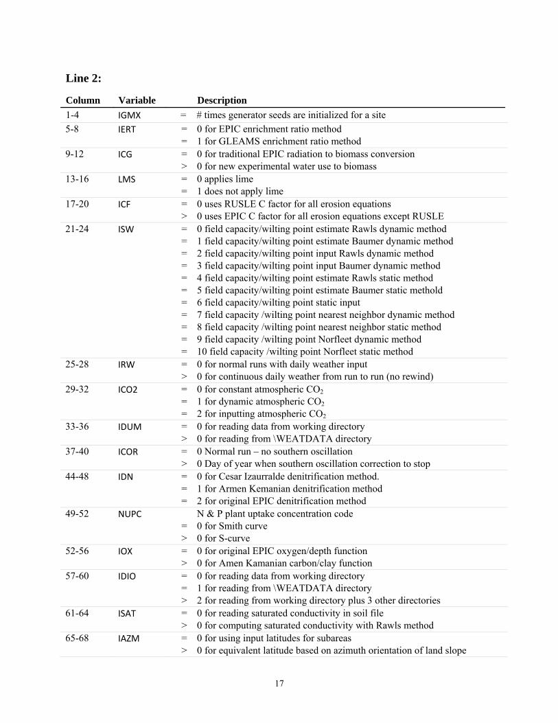
Line 2:


1-4 IGMX = # times generator seeds are initialized for a site

5-8 IERT = 0 for EPIC enrichment ratio method = 1 for GLEAMS enrichment ratio method 9-12 ICG = 0 for traditional EPIC radiation to biomass conversion > 0 for new experimental water use to biomass 13-16 LMS = 0 applies lime = 1 does not apply lime 17-20 ICF = 0 uses RUSLE C factor for all erosion equations > 0 uses EPIC C factor for all erosion equations except RUSLE 21-24 ISW = 0 field capacity/wilting point estimate Rawls dynamic method = 1 field capacity/wilting point estimate Baumer dynamic method = 2 field capacity/wilting point input Rawls dynamic method = 3 field capacity/wilting point input Baumer dynamic method = 4 field capacity/wilting point estimate Rawls static method = 5 field capacity/wilting point estimate Baumer static methold = 6 field capacity/wilting point static input = 7 field capacity /wilting point nearest neighbor dynamic method = 8 field capacity /wilting point nearest neighbor static method = 9 field capacity /wilting point Norfleet dynamic method = 10 field capacity /wilting point Norfleet static method 25-28 IRW = 0 for normal runs with daily weather input > 0 for continuous daily weather from run to run (no rewind) 29-32 ICO2 = 0 for constant atmospheric CO2 = 1 for dynamic atmospheric CO2 = 2 for inputting atmospheric CO2 33-36 IDUM = 0 for reading data from working directory > 0 for reading from \WEATDATA directory 37-40 ICOR = 0 Normal run – no southern oscillation > 0 Day of year when southern oscillation correction to stop 44-48 IDN = 0 for Cesar Izaurralde denitrification method. = 1 for Armen Kemanian denitrification method = 2 for original EPIC denitrification method 49-52 NUPC N & P plant uptake concentration code = 0 for Smith curve > 0 for S-curve 52-56 IOX = 0 for original EPIC oxygen/depth function > 0 for Amen Kamanian carbon/clay function 57-60 IDIO = 0 for reading data from working directory = 1 for reading from \WEATDATA directory > 2 for reading from working directory plus 3 other directories 61-64 ISAT = 0 for reading saturated conductivity in soil file > 0 for computing saturated conductivity with Rawls method 65-68 IAZM = 0 for using input latitudes for subareas > 0 for equivalent latitude based on azimuth orientation of land slope

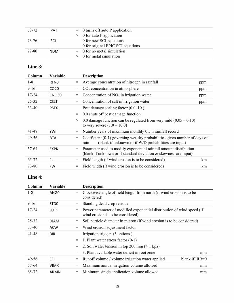
18

68-72 IPAT = 0 turns off auto P application > 0 for auto P application 73-76 ISCI 0 for new SCI equations 0 for original EPIC SCI equations 77-80 NDM = 0 for no metal simulation > 0 for metal simulation

Line 3:


1-8 RFN0 = Average concentration of nitrogen in rainfall ppm

9-16 CO20 = CO2 concentration in atmosphere ppm

17-24 CNO30 = Concentration of NO3 in irrigation water ppm

25-32 CSLT = Concentration of salt in irrigation water ppm

33-40 PSTX Pest damage scaling factor (0.0–10.)

= 0.0 shuts off pest damage function.

> 0.0 damage function can be regulated from very mild (0.05 – 0.10) to very severe (1.0 – 10.0)

41-48 YWI = Number years of maximum monthly 0.5 h rainfall record

49-56 BTA = Coefficient (0-1) governing wet-dry probabilities given number of days of rain (blank if unknown or if W/D probabilities are input)

57-64 EXPK = Parameter used to modify exponential rainfall amount distribution (blank if unknown or if standard deviation & skewness are input)

65-72 FL = Field length (if wind erosion is to be considered) km

73-80 FW = Field width (if wind erosion is to be considered) km

Line 4:


1-8 ANG0 = Clockwise angle of field length from north (if wind erosion is to be considered)

9-16 STD0 = Standing dead crop residue

17-24 UXP = Power parameter of modified exponential distribution of wind speed (if wind erosion is to be considered)

25-32 DIAM = Soil particle diameter in micron (if wind erosion is to be considered)

33-40 ACW = Wind erosion adjustment factor

41-48 BIR Irrigation trigger (3 options )

= 1. Plant water stress factor (0-1)

= 2. Soil water tension in top 200 mm (> 1 kpa)

= 3. Plant available water deficit in root zone mm

49-56 EFI = Runoff volume / volume irrigation water applied blank if IRR=0

57-64 VIMX = Maximum annual irrigation volume allowed mm

65-72 ARMN = Minimum single application volume allowed mm

19

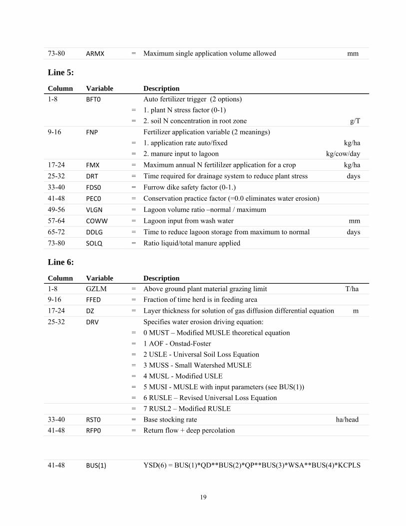
73-80 ARMX = Maximum single application volume allowed mm

Line 5:


1-8 BFT0 Auto fertilizer trigger (2 options)

= 1. plant N stress factor (0-1)

= 2. soil N concentration in root zone g/T

9-16 FNP Fertilizer application variable (2 meanings)

= 1. application rate auto/fixed kg/ha

= 2. manure input to lagoon kg/cow/day

17-24 FMX = Maximum annual N fertililzer application for a crop kg/ha

25-32 DRT = Time required for drainage system to reduce plant stress days

33-40 FDS0 = Furrow dike safety factor (0-1.)

41-48 PEC0 = Conservation practice factor (=0.0 eliminates water erosion)

49-56 VLGN = Lagoon volume ratio –normal / maximum

57-64 COWW = Lagoon input from wash water mm

65-72 DDLG = Time to reduce lagoon storage from maximum to normal days

73-80 SOLQ = Ratio liquid/total manure applied

Line 6:


1-8 GZLM = Above ground plant material grazing limit T/ha

9-16 FFED = Fraction of time herd is in feeding area

17-24 DZ = Layer thickness for solution of gas diffusion differential equation m

25-32 DRV Specifies water erosion driving equation:

= 0 MUST – Modified MUSLE theoretical equation

= 1 AOF - Onstad-Foster

= 2 USLE - Universal Soil Loss Equation

= 3 MUSS - Small Watershed MUSLE

= 4 MUSL - Modified USLE

= 5 MUSI - MUSLE with input parameters (see BUS(1))

= 6 RUSLE – Revised Universal Loss Equation

= 7 RUSL2 – Modified RUSLE

33-40 RST0 = Base stocking rate ha/head

41-48 RFP0 = Return flow + deep percolation

41-48 BUS(1) YSD(6) = BUS(1)*QD**BUS(2)*QP**BUS(3)*WSA**BUS(4)*KCPLS

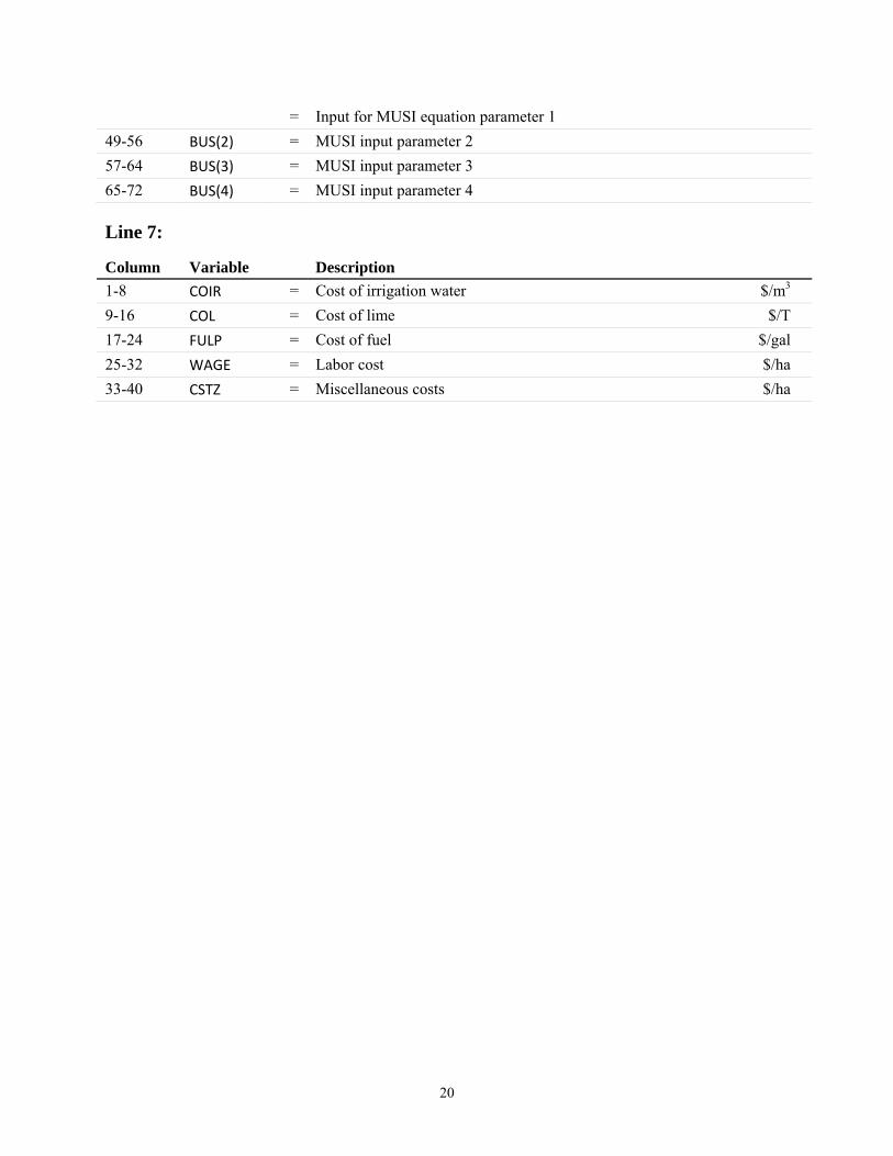
20

= Input for MUSI equation parameter 1

49-56 BUS(2) = MUSI input parameter 2



Line 7:


1-8 COIR = Cost of irrigation water $/m3

9-16 COL = Cost of lime $/T

17-24 FULP = Cost of fuel $/gal

25-32 WAGE = Labor cost $/ha

33-40 CSTZ = Miscellaneous costs $/ha

21

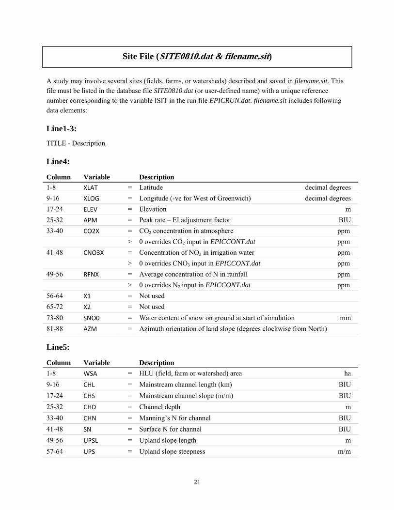
Site File (SITE0810.dat & filename.sit)

A study may involve several sites (fields, farms, or watersheds) described and saved in filename.sit. This file must be listed in the database file SITE0810.dat (or user-defined name) with a unique reference number corresponding to the variable ISIT in the run file EPICRUN.dat. filename.sit includes following data elements:

Line1-3:

TITLE - Description.

Line4:


1-8 XLAT = Latitude decimal degrees

9-16 XLOG = Longitude (-ve for West of Greenwich) decimal degrees

17-24 ELEV = Elevation m

25-32 APM = Peak rate – EI adjustment factor BIU

33-40 CO2X = CO2 concentration in atmosphere ppm

> 0 overrides CO2 input in EPICCONT.dat ppm

41-48 CNO3X = Concentration of NO3 in irrigation water ppm

> 0 overrides CNO3 input in EPICCONT.dat ppm

49-56 RFNX = Average concentration of N in rainfall ppm

> 0 overrides N2 input in EPICCONT.dat ppm

56-64 X1 = Not used

65-72 X2 = Not used

73-80 SNO0 = Water content of snow on ground at start of simulation mm

81-88 AZM = Azimuth orientation of land slope (degrees clockwise from North)

Line5:


1-8 WSA = HLU (field, farm or watershed) area ha

9-16 CHL = Mainstream channel length (km) BIU

17-24 CHS = Mainstream channel slope (m/m) BIU

25-32 CHD = Channel depth m

33-40 CHN = Manning’s N for channel BIU

41-48 SN = Surface N for channel BIU

49-56 UPSL = Upland slope length m

57-64 UPS = Upland slope steepness m/m

22

65-72 PEC = Conservation practice factor (=0.0 eliminates water erosion)

73-80 DTG = Time interval for gas diffusion equations h

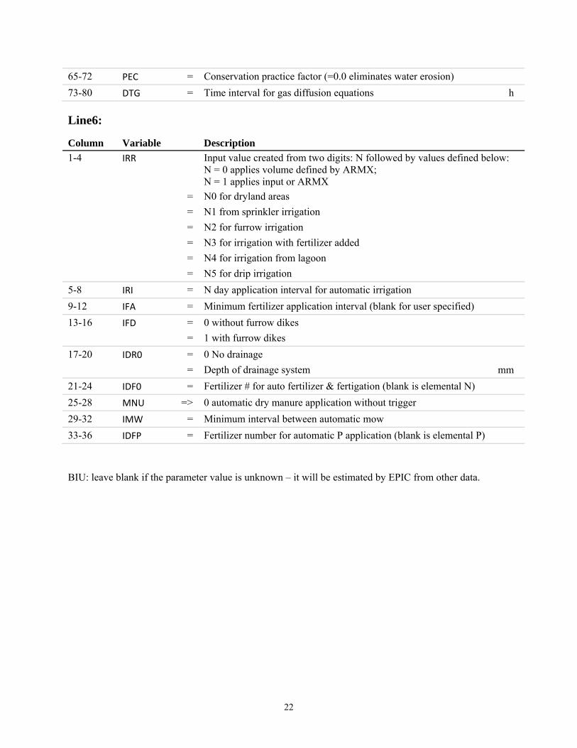
Line6:


1-4 IRR Input value created from two digits: N followed by values defined below: N = 0 applies volume defined by ARMX; N = 1 applies input or ARMX

= N0 for dryland areas

= N1 from sprinkler irrigation

= N2 for furrow irrigation

= N3 for irrigation with fertilizer added

= N4 for irrigation from lagoon

= N5 for drip irrigation

5-8 IRI = N day application interval for automatic irrigation

9-12 IFA = Minimum fertilizer application interval (blank for user specified)

13-16 IFD = 0 without furrow dikes

= 1 with furrow dikes

17-20 IDR0 = 0 No drainage

= Depth of drainage system mm

21-24 IDF0 = Fertilizer # for auto fertilizer & fertigation (blank is elemental N)

25-28 MNU => 0 automatic dry manure application without trigger

29-32 IMW = Minimum interval between automatic mow

33-36 IDFP = Fertilizer number for automatic P application (blank is elemental P)

BIU: leave blank if the parameter value is unknown – it will be estimated by EPIC from other data.

23

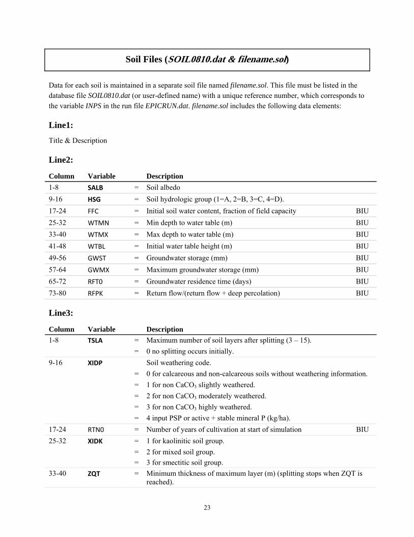
Soil Files (SOIL0810.dat & filename.sol)

Data for each soil is maintained in a separate soil file named filename.sol. This file must be listed in the database file SOIL0810.dat (or user-defined name) with a unique reference number, which corresponds to the variable INPS in the run file EPICRUN.dat. filename.sol includes the following data elements:

Line1:

Title & Description

Line2:


1-8 SALB = Soil albedo

9-16 HSG = Soil hydrologic group (1=A, 2=B, 3=C, 4=D).

17-24 FFC = Initial soil water content, fraction of field capacity BIU

25-32 WTMN = Min depth to water table (m) BIU

33-40 WTMX = Max depth to water table (m) BIU

41-48 WTBL = Initial water table height (m) BIU

49-56 GWST = Groundwater storage (mm) BIU

57-64 GWMX = Maximum groundwater storage (mm) BIU

65-72 RFT0 = Groundwater residence time (days) BIU

73-80 RFPK = Return flow/(return flow + deep percolation) BIU

Line3:


1-8 TSLA = Maximum number of soil layers after splitting (3 – 15).

= 0 no splitting occurs initially.

9-16 XIDP Soil weathering code.

= 0 for calcareous and non-calcareous soils without weathering information.

= 1 for non CaCO3 slightly weathered.

= 2 for non CaCO3 moderately weathered.

= 3 for non CaCO3 highly weathered.

= 4 input PSP or active + stable mineral P (kg/ha).

17-24 RTN0 = Number of years of cultivation at start of simulation BIU

25-32 XIDK = 1 for kaolinitic soil group.

= 2 for mixed soil group.

= 3 for smectitic soil group.

33-40 ZQT = Minimum thickness of maximum layer (m) (splitting stops when ZQT is reached).

24

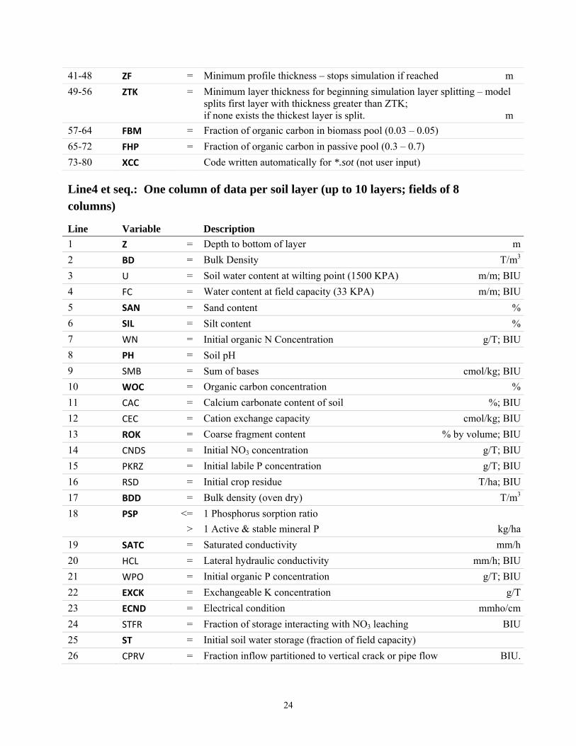
41-48 ZF = Minimum profile thickness – stops simulation if reached m

49-56 ZTK = Minimum layer thickness for beginning simulation layer splitting – model splits first layer with thickness greater than ZTK; if none exists the thickest layer is split. m

57-64 FBM = Fraction of organic carbon in biomass pool (0.03 – 0.05)

65-72 FHP = Fraction of organic carbon in passive pool (0.3 – 0.7)

73-80 XCC Code written automatically for *.sot (not user input)

Line4 et seq.: One column of data per soil layer (up to 10 layers; fields of 8 columns)

Line Variable Description

1 Z = Depth to bottom of layer m

2 BD = Bulk Density T/m3

3 U = Soil water content at wilting point (1500 KPA) m/m; BIU

4 FC = Water content at field capacity (33 KPA) m/m; BIU

5 SAN = Sand content %

6 SIL = Silt content %

7 WN = Initial organic N Concentration g/T; BIU

8 PH = Soil pH

9 SMB = Sum of bases cmol/kg; BIU

10 WOC = Organic carbon concentration %

11 CAC = Calcium carbonate content of soil %; BIU

12 CEC = Cation exchange capacity cmol/kg; BIU

13 ROK = Coarse fragment content % by volume; BIU

14 CNDS = Initial NO3 concentration g/T; BIU

15 PKRZ = Initial labile P concentration g/T; BIU

16 RSD = Initial crop residue T/ha; BIU

17 BDD = Bulk density (oven dry) T/m3

18 PSP <= 1 Phosphorus sorption ratio

> 1 Active & stable mineral P kg/ha

19 SATC = Saturated conductivity mm/h

20 HCL = Lateral hydraulic conductivity mm/h; BIU

21 WPO = Initial organic P concentration g/T; BIU

22 EXCK = Exchangeable K concentration g/T

23 ECND = Electrical condition mmho/cm

24 STFR = Fraction of storage interacting with NO3 leaching BIU

25 ST = Initial soil water storage (fraction of field capacity)

26 CPRV = Fraction inflow partitioned to vertical crack or pipe flow BIU.

25

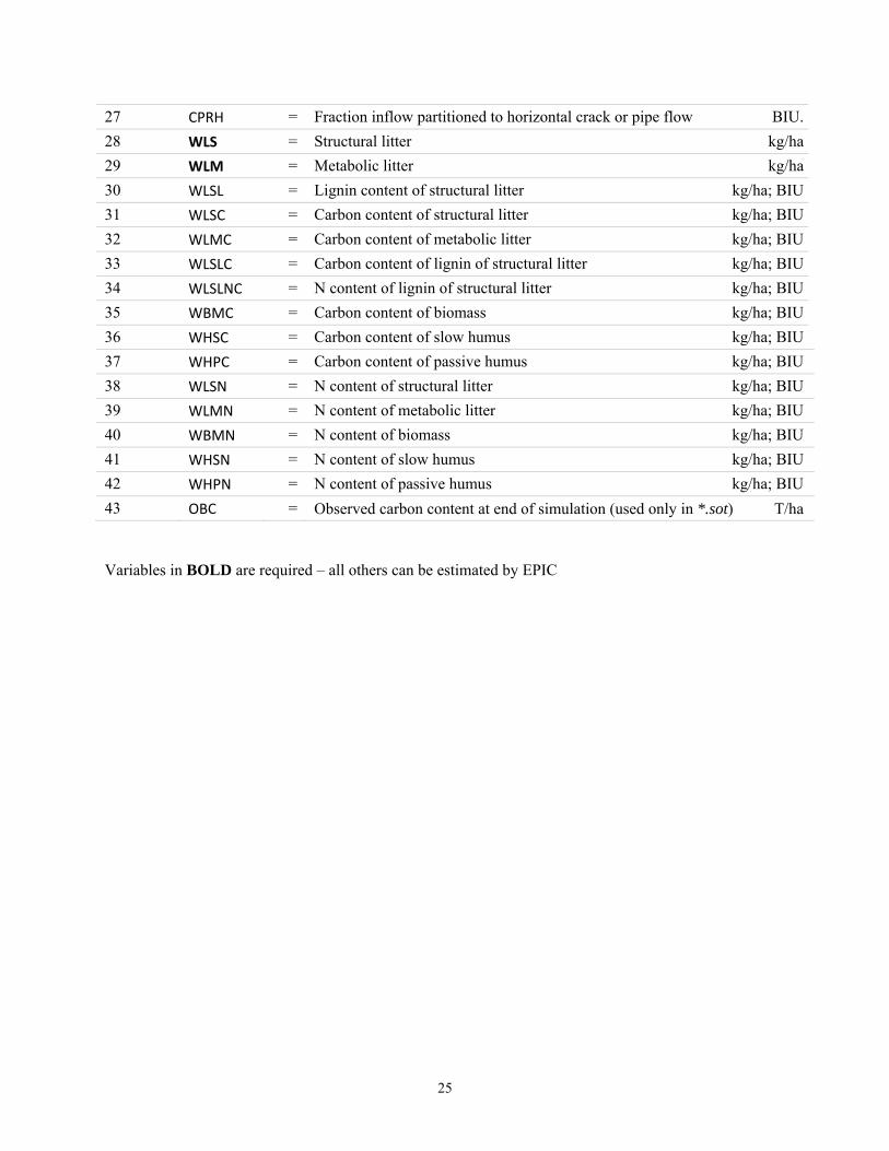
27 CPRH = Fraction inflow partitioned to horizontal crack or pipe flow BIU.

28 WLS = Structural litter kg/ha

29 WLM = Metabolic litter kg/ha

30 WLSL = Lignin content of structural litter kg/ha; BIU

31 WLSC = Carbon content of structural litter kg/ha; BIU

32 WLMC = Carbon content of metabolic litter kg/ha; BIU

33 WLSLC = Carbon content of lignin of structural litter kg/ha; BIU

34 WLSLNC = N content of lignin of structural litter kg/ha; BIU

35 WBMC = Carbon content of biomass kg/ha; BIU

36 WHSC = Carbon content of slow humus kg/ha; BIU

37 WHPC = Carbon content of passive humus kg/ha; BIU

38 WLSN = N content of structural litter kg/ha; BIU

39 WLMN = N content of metabolic litter kg/ha; BIU

40 WBMN = N content of biomass kg/ha; BIU

41 WHSN = N content of slow humus kg/ha; BIU

42 WHPN = N content of passive humus kg/ha; BIU

43 OBC = Observed carbon content at end of simulation (used only in *.sot) T/ha

Variables in BOLD are required – all others can be estimated by EPIC

26

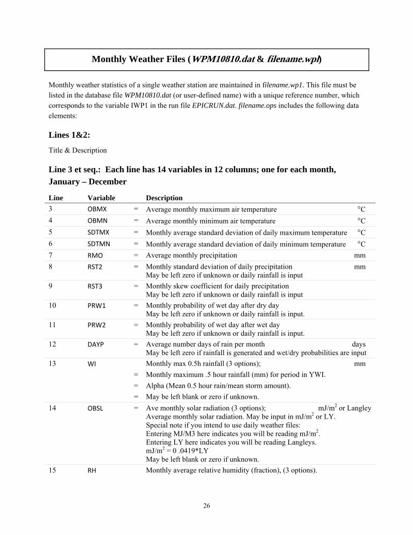
Monthly Weather Files (WPM10810.dat & filename.wpl)

Monthly weather statistics of a single weather station are maintained in filename.wp1. This file must be listed in the database file WPM10810.dat (or user-defined name) with a unique reference number, which corresponds to the variable IWP1 in the run file EPICRUN.dat. filename.ops includes the following data elements:

Lines 1&2:

Title & Description

Line 3 et seq.: Each line has 14 variables in 12 columns; one for each month, January – December


3 OBMX = Average monthly maximum air temperature °C

4 OBMN = Average monthly minimum air temperature °C

5 SDTMX = Monthly average standard deviation of daily maximum temperature °C

6 SDTMN = Monthly average standard deviation of daily minimum temperature °C

7 RMO = Average monthly precipitation mm

8 RST2 = Monthly standard deviation of daily precipitation mm May be left zero if unknown or daily rainfall is input

9 RST3 = Monthly skew coefficient for daily precipitation May be left zero if unknown or daily rainfall is input

10 PRW1 = Monthly probability of wet day after dry day May be left zero if unknown or daily rainfall is input.

11 PRW2 = Monthly probability of wet day after wet day May be left zero if unknown or daily rainfall is input.

12 DAYP = Average number days of rain per month days May be left zero if rainfall is generated and wet/dry probabilities are input

13 WI Monthly max 0.5h rainfall (3 options); mm

= Monthly maximum .5 hour rainfall (mm) for period in YWI.

= Alpha (Mean 0.5 hour rain/mean storm amount).

= May be left blank or zero if unknown.

14 OBSL = Ave monthly solar radiation (3 options); mJ/m2 or Langley Average monthly solar radiation. May be input in mJ/m2 or LY. Special note if you intend to use daily weather files: Entering MJ/M3 here indicates you will be reading mJ/m2. Entering LY here indicates you will be reading Langleys. mJ/m2 = 0 .0419*LY May be left blank or zero if unknown.

15 RH Monthly average relative humidity (fraction), (3 options).

27

= 1. Average Monthly relative humidity (Fraction, e.g. 0.75)

= 2. Average Monthly dew point temp °C

= 3. Blanks or zeros if unknown.

NOTE: May be left zero unless a PENMAN equation is used to estimate potential evaporation see variable IET.

16 UAV0 = Average monthly wind speed m/s

The WPM50810.dat file has the same format.

28

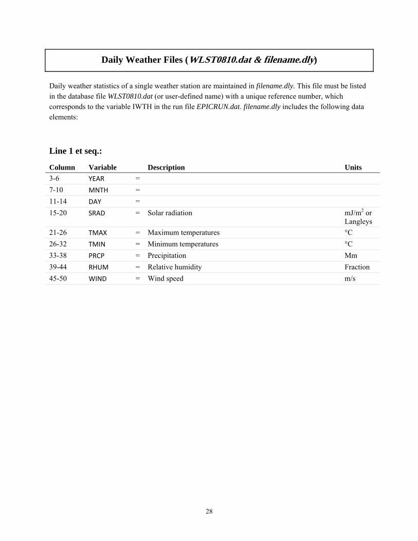
Daily Weather Files (WLST0810.dat & filename.dly)

Daily weather statistics of a single weather station are maintained in filename.dly. This file must be listed in the database file WLST0810.dat (or user-defined name) with a unique reference number, which corresponds to the variable IWTH in the run file EPICRUN.dat. filename.dly includes the following data elements:

Line 1 et seq.:

Column Variable Description Units

3-6 YEAR =

7-10 MNTH =

11-14 DAY =

15-20 SRAD = Solar radiation mJ/m2 or Langleys

21-26 TMAX = Maximum temperatures °C

26-32 TMIN = Minimum temperatures °C

33-38 PRCP = Precipitation Mm

39-44 RHUM = Relative humidity Fraction

45-50 WIND = Wind speed m/s

29

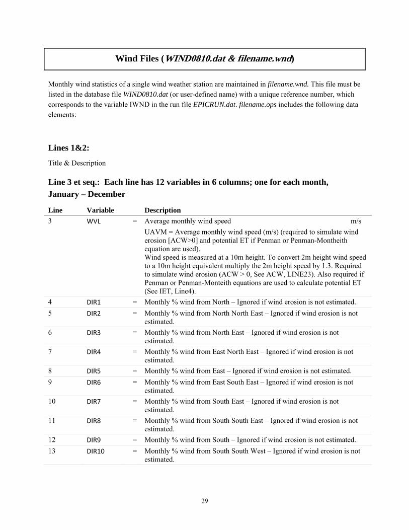
Wind Files (WIND0810.dat & filename.wnd)

Monthly wind statistics of a single wind weather station are maintained in filename.wnd. This file must be listed in the database file WIND0810.dat (or user-defined name) with a unique reference number, which corresponds to the variable IWND in the run file EPICRUN.dat. filename.ops includes the following data elements:

Lines 1&2:

Title & Description

Line 3 et seq.: Each line has 12 variables in 6 columns; one for each month, January – December


3 WVL = Average monthly wind speed m/s

UAVM = Average monthly wind speed (m/s) (required to simulate wind erosion [ACW>0] and potential ET if Penman or Penman-Montheith equation are used). Wind speed is measured at a 10m height. To convert 2m height wind speed to a 10m height equivalent multiply the 2m height speed by 1.3. Required to simulate wind erosion (ACW > 0, See ACW, LINE23). Also required if Penman or Penman-Monteith equations are used to calculate potential ET (See IET, Line4).

4 DIR1 = Monthly % wind from North – Ignored if wind erosion is not estimated.

5 DIR2 = Monthly % wind from North North East – Ignored if wind erosion is not estimated.

6 DIR3 = Monthly % wind from North East – Ignored if wind erosion is not estimated.

7 DIR4 = Monthly % wind from East North East – Ignored if wind erosion is not estimated.

8 DIR5 = Monthly % wind from East – Ignored if wind erosion is not estimated.

9 DIR6 = Monthly % wind from East South East – Ignored if wind erosion is not estimated.

10 DIR7 = Monthly % wind from South East – Ignored if wind erosion is not estimated.

11 DIR8 = Monthly % wind from South South East – Ignored if wind erosion is not estimated.

12 DIR9 = Monthly % wind from South – Ignored if wind erosion is not estimated.

13 DIR10 = Monthly % wind from South South West – Ignored if wind erosion is not estimated.

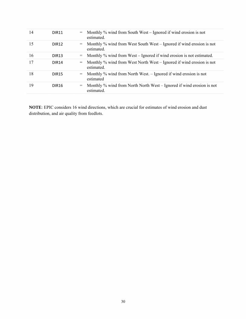
30

14 DIR11 = Monthly % wind from South West – Ignored if wind erosion is not estimated.

15 DIR12 = Monthly % wind from West South West – Ignored if wind erosion is not estimated.

16 DIR13 = Monthly % wind from West – Ignored if wind erosion is not estimated.

17 DIR14 = Monthly % wind from West North West – Ignored if wind erosion is not estimated.

18 DIR15 = Monthly % wind from North West. – Ignored if wind erosion is not estimated

19 DIR16 = Monthly % wind from North North West – Ignored if wind erosion is not estimated.

NOTE: EPIC considers 16 wind directions, which are crucial for estimates of wind erosion and dust distribution, and air quality from feedlots.

31

How to Prepare Weather Input Files

Historical daily weather data can be used in two ways: First, these data can be directly used in EPIC simulation when the length of historical daily weather is the same as the simulation period. Second, in general the historical daily weather data are primarily used to generate monthly weather data, which then are used to generate EPIC weather input data. The format for historical daily weather data is explained below:

Line1:

Weather file name

Line2:

Number of the years in the actual daily weather data (col.1-4) followed by the beginning year. For example: 131981 means that there are 13 years of weather data beginning with year of 1981.

Line3:

From this line forward, every line includes nine variables. These nine variables are:

Column Variable

1-6 Year 7-10 Month 11-14 Day 15-20 Solar Radiation 21-26 Maximum temperature 27-32 Minimum temperature 33-38 Precipitation 39-44 Relative humidity 45-50 Wind velocity

After completing the following steps to develop the WPM10810.dat file, if any daily record of maximum temperature, minimum temperature, or precipitation are missing, enter 9999.0 in the missing field(s) of the record(s). EPIC will generate the missing record automatically when using measured weather in a simulation.

NOTE: DO NOT USE 9999.0 FOR ANY RECORD BEFORE DEVELOPING THE WPM10810.dat BELOW.

Format of Daily Weather Input Files

The easiest way to build a historical daily weather input file is to enter the data in an Excel spreadsheet and then save it as *.prn file and rename the *.prn file to a *.txt file. The included EPIC weather program WXGN3020.exe will read this *.txt file to create the generated monthly weather file (*.wp1).

32

Run EPIC Weather Program

Put the historical daily weather input file under the weather program directory. Before starting to run the weather generating program (WXGN3020.exe), one needs to set up WXGNRUN.dat file. This can be done by putting the actual daily weather file name (*.dly) on the first line in WXGNRUN.dat file if only one weather data set needs to be generated. In the event of several weather data sets need to be generated by WXGN3020.exe, each individual actual daily weather data set name has to be listed in WXGNRUN.dat file. By doing so, the WXGN3020.exe will read all the daily weather files listed in WXGNRUN.dat and generate all the monthly weather files. When WXGNRUN.dat is set up, one can execute the weather generation program by typing WXGN3020 under the appropriate driver path prompt where both actual daily weather and weather generating program are stored. Then press ENTER key. The weather program will start to run until it is finished. When it is finished, it produces three files: *.DLY (an actual daily weather file), *.OUT, and *.INP files. In which only *.INP file is needed for EPIC simulation. To be consistent, this *.INP file should be renamed as *.WP1. The *.WP1 file will be listed in the weather list file (WPM10810.dat). For the content of *.WP1 file, please refer to the next section of WPM10810.dat.

33

Operation Schedule Files (OPSC0810.dat & filename.ops)

Data of field operation schedules are maintained in a separate file named filename.ops. This file must be listed in the database file OPSC0810.data (or user-defined name) with a unique reference number, which corresponds to the variable IOPS in the run file EPICRUN.dat. filename.ops includes the following data elements:

Line1:

Title & Description

Line2:


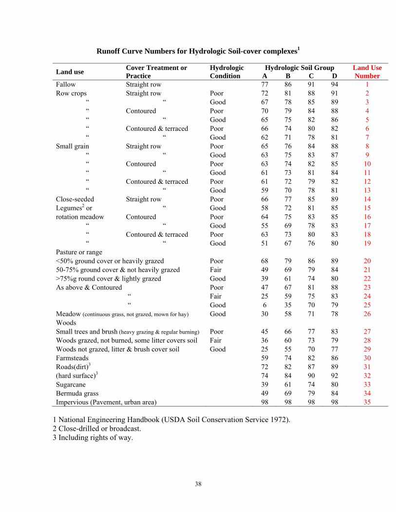
1-4 LUN = Land use number from NRCS Land Use-Hydrologic Soil Group Table Refer to the column labeled Land User Number in the table on Page 33. This number along with the hydrologic soil group is used to determine the curve number. (Range: 1-35)

5-8 IAUI = Auto irrigation; apply irrigation operation from TILL0810.dat (Range: 1-∞). If auto irrigation is used, this irrigation operation (found in the TILL0810.dat file) will be used to apply irrigation water. If none is specified, the default is operation #500.

Line3 et seq.: (one line per operation)


1-3 IYEAR = Year of operation (Range: 1–N)

4-6 MON = Month of operation (Range 1-12)

7-9 DAY = Day of operation (Range: 1-31) NOTE It is recommended not to schedule something for 29 February.

10-14 CODE = Tillage ID number (Refers to the ID number that is given to each tillage operation or piece of equipment in TILL0810.dat)

15-19 TRAC = Tractor ID number (Refers to the ID number given to each tractor in TILL0810.dat) NOTE This may be omitted if economic analysis is not required

20-24 CRP = Crop ID number (Refers to the crop ID number given to each crop as listed in CROP0810.dat)

25-29 XMTU = Time from planting to maturity in Years (for tree crops only)

= Time from planting to harvest in Years (for tree crops at planting only). This refers to the time to complete maturity of the tree (full life of the tree). No potential heat units are entered for trees. This value is calculated from XMTU (Range: 5-300)

34

LYR = Time from planting to harvest in years, if JX(4) is a harvest operation for trees (proportion of full maturity) (Range: 5-100)

= Pesticide ID number from PEST0810.dat (for pesticide application only)

= Fertilizer ID number from FERT0810.dat (for fertilizer application only)

30-37 OPV1 = Potential heat units (PHU) from germination required by the plant to reach maturity. Total number of heat units or growing degree days needed to bring the plant from emergence to physiological maturity. Used in determining the growth curve. Enter 0 if unknown. (Range: 1-5000) NOTE For trees, no PHU are entered. They are calculated from XMTU. For

crops other than trees PHU are accumulated annually and reset to 0 at the end of the year. Trees are a special case in which PHUs continue to accumulate from year to year. Deciduous trees are also a special case within trees in which PHUs are calculated annually (similar to non-tree crops) in order to simulate leaf drop as well as accumulate PHUs from year to year to simulate the maturity of the tree.

= Application volume in mm for irrigation. (Range: 1-5000)

= Fertilizer application rate in kg/ha; For variable rate set equal to 0. (Range: 0-500)

= Pesticide application rate in kg/ha. (Range: 0-500)

= Stocking rate for grazing in ha/head. On a Start Grazing operation this variable is used to set the stocking rate in number of hectares/animal. Using this feature, the user can change the number of animals in the herd at any point in time simulating buying/selling of animals. (Range: 0-200)

38-45 OPV2 = Two (2) condition SCS Runoff Curve number, or Land Use number (optional) . The land use number set previously can be overridden at this point if an operation has caused the land condition to change. (Range: 1-35)

= Fraction of pests controlled by pesticide application. This factor is used to control pest populations by applying pesticides. It only applies to insects and diseases. Weeds are handled through intercropping. (Range: 0-1) NOTE If this factor is set to 0.99, 99% of the pests will be killed. After each

treatment, the population will begin to regrow based on several parameters set in the Control file (PSTX), Crop file (PST) and Parm file (parms 9 & 10).

Currently the model is set so that very minimal damage is caused by pests and therefore does not reduce yield. Pest growth is dependent on temperature and humidity. Warm and wet conditions favor pest growth while dry and cool conditions inhibit pest growth.

35

46-53 OPV3 = Automatic Irrigation Trigger This is the same irrigation trigger function as in the control file. The control file value can be overridden by setting the trigger value in the operation schedule. Leaving OPV3 = 0 no modifications will be made to the irrigation trigger as set in the control file. To trigger automatic irrigation, the water stress factor is set: = 0 - Manual irrigation or model uses BIR set in control file

(EPICCONT.dat) = 0-1.0 - Plant water stress factor. (1 – BIR) equals the fraction of plant

water stress allowed 1.0 Does not allow water stress < 0.0 - Plant available water deficit in root zone (number is in mm and

must be negative) > 1.0 - Soil water tension in top 200mm (Absolute number is in

kilopascals) = 1000 - Sets water deficit high enough that only manual irrigations will

occur. This effectively turns auto irrigation off. NOTE When using a BIR based on anything other than plant water stress (0-

1), be aware that irrigation will be applied outside of the growing season if the soil water deficit or soil water tension reaches BIR. This will reduce the amount of water available for irrigation during the growing season.

Once the trigger has been set within a operation schedule, it will remain in effect until changed within the operation schedule. If the schedule is used in rotation with other schedules, the trigger will stay as set even into the next schedule. When setting the irrigation trigger within an operation schedule, it is wise to set the irrigation trigger to -1000 mm at the end of the schedule so that when the operation schedule is used in rotation with another non-automatically irrigated crop, the second crop is not influenced by the irrigation trigger.

54-61 OPV4 = Proportion of irrigation water applied lost to runoff (vol/vo)l. Setting the runoff fraction (EFI) within the operation schedule overrides the EFI set within the control file. The irrigation runoff ratio specifies the fraction of each irrigation application that is lost to runoff. Soluble nutrient loss through runoff applies. Changes in soil slope do not affect this amount dynamically. (Range: 0-1)

62-69 OPV5 = Plant population at planting (plants/m2 for small plants; plants/ha for larger plants with densities < 1/m2, e.g. trees). NOTE EPIC does not simulate tillering. In crops such as wheat and sugarcane

which produce higher numbers of yielding tillers compared to the number of seeds or shoots planted, the plant population must be estimated based on the final yield producing tiller number. (Range: 0-500)

70-77 OPV6 = Maximum annual N fertilizer applied to a crop = 0 (or blank) does not change FMX (EPICCONT.dat)

36

> 0 sets new FMX for planting only. In the control file FMX was set to limit the amount of fertilizer that could be applied on an annual basis regardless of the number of crops grown within a year. Refer to FMX (page 17) for further information. The maximum annual amount of nitrogen fertilizer can also be set here in the operation schedule and can be set per crop so that each crop has a specified amount of nitrogen fertilizer available to it. This is especially important when automatically applying fertilizer. NOTE If this variable is set either in the control file or in the operation schedule and manual fertilization is applied, the model will only apply up to this maximum amount regardless of the amount specified in the manual fertilization operation.

78-85 OPV7 = Time of operation as fraction of growing season This is also referred to as heat unit scheduling. Heat unit scheduling can be used to schedule operations at a particular stage of growth. For example, irrigation could be scheduled at 0.25, 0.5, and 0.75 which might represent varying stages of crop growth. Irrigation would then be applied at 25%, 50%, and 75% of the potential heat units set at planting. Enter earliest possible Month & Day in JX(2) & JX(3). NOTE When setting up an operation using heat unit scheduling it is best to enter earliest possible Month and day ( JX(2) & JX(3)) that the operation could occur on because in order for the operation to occur the date of the operation as well as the number of heat units scheduled must be met. This is especially true for harvest operations. It is recommended that the harvest date be set 10-14 days before actual harvest is expected to occur. This is recommended so that the date of the operation will be met before the heat units are met. If the date is set too late and the heat units are met before the date of the operation is met, the crop will continue to grow longer than expected which can affect yield. EPIC first checks to see that the date of the operation has been met; then it checks to see if the fraction of heat units has been met as defined below:.

Date Heat Units Action

Date is met Heat unit fraction not met

Operation will not occur until heat units requirement is met

Date is not met

Het unit fraction met

Operation will occur as soon as date is met. Note: Excess GDUs will accumulate causing the operation to occur later in the growing cycle than expected

Date is met Heat unit fraction met

Operation will occur immediately

37

Heat unit scheduling can also be used to adjust operations to the weather (temperatures) from year to year. If heat units are not scheduled (set to 0), operations will occur on the date as scheduled in the operation schedule. They will occur on the same date every year the crop is grown. Heat unit scheduling operations which occur from planting to harvest are based on the heat units set at planting. Operations which occur before planting are based on the total annual heat units which are calculated by the model. For some grain crops an in-field dry-down period is allowed. It is expressed as a fraction of the total heat units set at planting. In most cases the dry-down period is 10% to 15% of the total heat units. If a dry-down period is required, heat unit schedule the harvest operation to occur at 1.10, 1.15 or another appropriate fraction. In the case of forage harvesting, the forage is actually harvested well before the crop reaches full maturity. In this case heat unit schedule the forage harvest to 0.55 or another appropriate fraction.

86-93 OPV8 = Minimum USLE C-Factor

94-101 OPV9 = Moisture content of grain required for harvest

NOTE:

Variables LYR, OPV1& OPV2 are context dependent, i.e. they have different meanings and variable names depending on the type of operation.

38

Runoff Curve Numbers for Hydrologic Soil-cover complexes1

Land use Cover Treatment or Practice

Hydrologic Condition

Hydrologic Soil Group Land Use Number A B C D

Fallow Straight row 77 86 91 94 1 Row crops Straight row Poor 72 81 88 91 2

“ “ Good 67 78 85 89 3 “ Contoured Poor 70 79 84 88 4 “ “ Good 65 75 82 86 5 “ Contoured & terraced Poor 66 74 80 82 6 “ “ Good 62 71 78 81 7

Small grain Straight row Poor 65 76 84 88 8 “ “ Good 63 75 83 87 9 “ Contoured Poor 63 74 82 85 10 “ “ Good 61 73 81 84 11 “ Contoured & terraced Poor 61 72 79 82 12 “ “ Good 59 70 78 81 13

Close-seeded Straight row Poor 66 77 85 89 14 Legumes2 or “ Good 58 72 81 85 15 rotation meadow Contoured Poor 64 75 83 85 16

“ “ Good 55 69 78 83 17 “ Contoured & terraced Poor 63 73 80 83 18 “ “ Good 51 67 76 80 19

Pasture or range <50% ground cover or heavily grazed Poor 68 79 86 89 20 50-75% ground cover & not heavily grazed Fair 49 69 79 84 21 >75%g round cover & lightly grazed Good 39 61 74 80 22 As above & Contoured Poor 47 67 81 88 23

“ Fair 25 59 75 83 24 “ Good 6 35 70 79 25

Meadow (continuous grass, not grazed, mown for hay) Good 30 58 71 78 26 Woods Small trees and brush (heavy grazing & regular burning) Poor 45 66 77 83 27 Woods grazed, not burned, some litter covers soil Fair 36 60 73 79 28 Woods not grazed, litter & brush cover soil Good 25 55 70 77 29 Farmsteads 59 74 82 86 30 Roads(dirt)3 72 82 87 89 31 (hard surface)3 74 84 90 92 32 Sugarcane 39 61 74 80 33 Bermuda grass 49 69 79 84 34 Impervious (Pavement, urban area) 98 98 98 98 35

1 National Engineering Handbook (USDA Soil Conservation Service 1972). 2 Close-drilled or broadcast. 3 Including rights of way.

39

Crop File (CROP0810.dat)

The crops database CROP0810.dat includes over 100 crops, including trees and other perennials. There are 59 parameters used to describe each crops’ growth characteristics. Those parameters are all listed in a single line in CROP0810.dat file which includes the following data elements:

Each Line:


1-5 CNUM Crop reference number

7-10 CPNM Crop name abbreviation

11-18 WA = Biomass-Energy Ratio (CO2 = 330ppm). This is the potential (unstressed) growth rate (including roots) per unit of intercepted photosynthetically active radiation. This parameter should be one of the last to be adjusted. Adjustments should be based on research results. This parameter can greatly change the rate of growth, incidence of stress during the season and the resultant yield. Care should be taken to make adjustments in the parameter only based on data with no drought, nutrient or temperature stress.

19-26 HI = Harvest index. This crop parameter should be based experimental data where crop stresses have been minimized to allow the crop to attain its potential. EPIC adjusts HI as water stress occurs from near flowering to maturity.

27-34 TOPC = Optimal temperature for plant growth. °C TB and TG are very stable for cultivars within a species. They should not be changed once they are determined for a species. Varietal or maturity type differences are accounted for by different sums of thermal units.

35-42 TBSC = Minimum temperature for plant growth. °C TB and TG are very stable for cultivars within a species. They should not be changed once they are determined for a species. Varietal or maturity type differences are accounted for by different sums of thermal units.

43-50 DMLA = Maximum potential leaf area index. The parameters in the CROP8190.dat data set are based on the highest expected plant densities for crops not expected to have water stress. DMLA is internally adjusted for drought-prone regions as planting densities are much smaller in these areas unless irrigation is used.

40

51-58 DLAI = Fraction of growing season when leaf area declines. The fraction of the growing season in heat units in divided by the total heat units accumulated between planting and crop maturity. If the date at which leaf area normally declines is known, one of the options in EPIC can be used to estimate the fraction of heat units accumulated. A multi-run EPIC simulation is setup with IGSD equal to 366. A one-year simulation followed by a one-year multi-run will produce a multi-run simulation, which has average heat units per month and the total heat units to maturity. The harvest date kill operations should be set to the crop maturity date. The estimated heat units at maximum leaf area can then be divided by the heat units at maturity to estimate the fraction of the growing season at which leaf-area index start to decline.

59-66 DLAP1 = First point on optimal leaf area development curve. Two points on optimal (nonstress) leaf area development curve. Numbers before decimal are % of growing season. Numbers after decimal are fractions of maximum potential LAI. Research results or observations on the % of maximum leaf area at two points in the development of leaf area can be used in conjunction with an EPIC simulation like that described for DLAI. The results of the one-year multi-run will establish the cumulative heat units by month from planting to maturity. Then calculate percent of cumulative heat units by dividing estimated cumulative heat units for each of the two dates where you've estimated percent of Max LAI by the average annual heat units shown on the bottom of the crop parameter set at the beginning of the EPIC run. NOTE: The percent of heat units for first monthly estimate is the number on the left of the decimal for DLAP1 and the estimated percent of the Max LAI is the number in the right of the decimal.

67-74 DLAP2 = Second point on optimal leaf area development curve. Two points on optimal (nonstress) leaf area development curve. Numbers before decimal are % of growing season. Numbers after decimal are fractions of maximum potential LAI. Research results or observations on the % of maximum leaf area at two points in the development of leaf area can be used in conjunction with an EPIC simulation like that described for DLAI. The results of the one-year multi-run will establish the cumulative heat units by month from planting to maturity. Then calculate percent of cumulative heat units by dividing estimated cumulative heat units for each of the two dates where you've estimated percent of Max LAI by the average annual heat units shown on the bottom of the crop parameter set at the beginning of the EPIC run. NOTE: The percent of heat units for second date estimate is the number on the left of the decimal for DLAP2 and the estimated percent of the Max LAI is the number in the right of the decimal.

75-82 RLAD = Leaf area index decline rate parameter. Leaf-area-index decline rate parameter (estimated LAI decline between DLAI and harvest) -1.0 is linear; > 1 accelerates decline; < 1 retards decline rate. Values range from 0 to 10.

41

83-90 RBMD = Biomass-energy ratio decline rate parameter Biomass-energy ratio decline rate parameter for late in the cropping season. This crop parameter functions like the RLAD above for values ranging from 0-10. It reduces the efficiency of conversion of intercepted photosynthetically active radiation to biomass due to production of high energy products like seeds and/or translocation of N from leaves to seeds.

91-98 ALT = Index of crop tolerance to aluminum saturation (1-5; 1=sensitive, 5=tolerant).

99-106 GSI = Maximum Stomatal Conductance m/s The crop parameter GSI is the maximum stomatal conductance (m/s) at high solar radiation and low vapor pressure deficit. Korner et al. (1979) reported maximum stomatal conductance values for 246 species and cultivars.

107-114 CAF = Critical aeration factor Fraction of soil porosity where poor aeration starts limiting plant growth. This is set at 0.85 for most crops, with rice being the major exception with a value of 1.0.

115-122 SDW = Seeding rate. Kg/ha Normal planting rate. Note this does not change the plant population. It only impacts seed cost and start crop biomass.

123-130 HMX = Maximum crop height in m.

131-138 RDMX = Maximum root depth in m. This effects soil moisture extraction.

139-146 WAC2 = CO2 Concentration /Resulting WA value (Split Variable). In EPIC, radiation use efficiency is sensitive to atmospheric CO2

concentration. WAC2 is an "S" curve parameter used to describe the effect of CO2 concentration on the crop parameter WA. The value on the left of the decimal is a value of CO2 concentration higher that ambient (i.e., 450 or 660 ul/l). The value on the right of the decimal is the corresponding value WA. This elevated value of WA can be estimated from experimental data on short-term crop growth at elevated CO2 levels. Calculate the ratio of crop growth rate at elevated CO2 to crop growth at approximately 330 ul l-1 CO2. Multiply that ratio by the value of WA at 330 ul l-1 to obtain the value on the right of the decimal. Typical values of the ratio are 1.1 to 1.2, 1.15 used in crop8190. for crops with the C4 photosynthetic pathway and 1.3 to 1.4, 1.35 used in crop8190 for C3 crops. (Kimball, B.A. 1983 Carbon dioxide and agricultural yield: an assemblage and analysis of 770 prior observations. Water Conservation Laboratory Report 14. USDA/ARS. Phoenix, Arizona).

147-154 CNY = Fraction of nitrogen in yield. g/g Normal fraction N in yield. This was estimated from Morrison's Feeds and Feeding and other data sources plant nutrition. The percentage N in Morrison was adjusted to a dry weight by dividing by the fraction of dry matter to total yield.

155-162 CPY = Fraction of phosphorus in yield. g/g Normal fraction of P in yield. Estimated by same procedure as CNY above.

163-170 CKY = Fraction of K in yield g/g

42

171-178 WSYF = Lower limit of harvest index. Fraction between 0 and HI value that represents the lowest harvest index expected due to water stress. A few crops can have slight increases in harvest index ie. the sugar content is higher in somewhat stressed sugar crops.

179-186 PST = Pest damage factor (insects, weeds, disease) Fraction of yield remaining after damage. Usually set at 0.60. EPIC has an adjustment process that is function of moisture, temperature and residue. This presently is a reasonable estimate, but future versions may include more detailed procedures. You may wish to adjust the parameter in geographic areas known to have large amounts of damage from pests.

187-194 CSTS = Seed cost $/kg

195-202 PRYG = Price for yield $/T

203-210 PRYF = Price for forage yield $/T

211-218 WCY = Fraction water in yield.

219-226 BN1 = Nitrogen uptake parameter (N fraction in plant at emergence). Normal fraction of N in crop biomass at emergence -This parameter is based on research results published in the literature for this or a similar crop.

227-234 BN2 = Nitrogen uptake parameter (N fraction in plant at 0.5 maturity). Normal fraction of N in crop biomass at mid-season -Same as BN1.

235-242 BN3 = Nitrogen uptake parameter (N fraction in plant at maturity). Normal fraction of N in crop biomass at maturity -Same as BN1.

243-250 BP1 = Phosphorus uptake parameter (P fraction in plant at emergence). Normal fraction of P in crop biomass at emergence -Same as BN1.

251-258 BP2 = Phosphorus uptake parameter (P fraction in plant at 0.5 maturity). Normal fraction of P in crop biomass at mid-season -Same as BN1.

259-266 BP3 = Phosphorus uptake parameter (P fraction in plant at maturity). Normal fraction of P in crop biomass at maturity -Same as BN1.

267-274 BK1 = K uptake at emergence

275-282 BK2 = K uptake at 0.5 maturity

283-290 BK3 = K uptake at maturity

291-298 BW1 = Wind erosion factor for standing live biomass Based on the Manhattan wind erosion equations for this crop or a similar crop used in the Manhattan wind erosion equations.

299-306 BW2 = Wind erosion factor for standing dead crop residue Same as BW1.

307-314 BW3 = Wind erosion factor for flat residue Same as BW1.

315-322 IDC Crop category number:

= 1 - Warm season annual legume.

= 2 - Cold season annual legume.

= 3 - Perennial legume.

= 4 - Warm season annual.

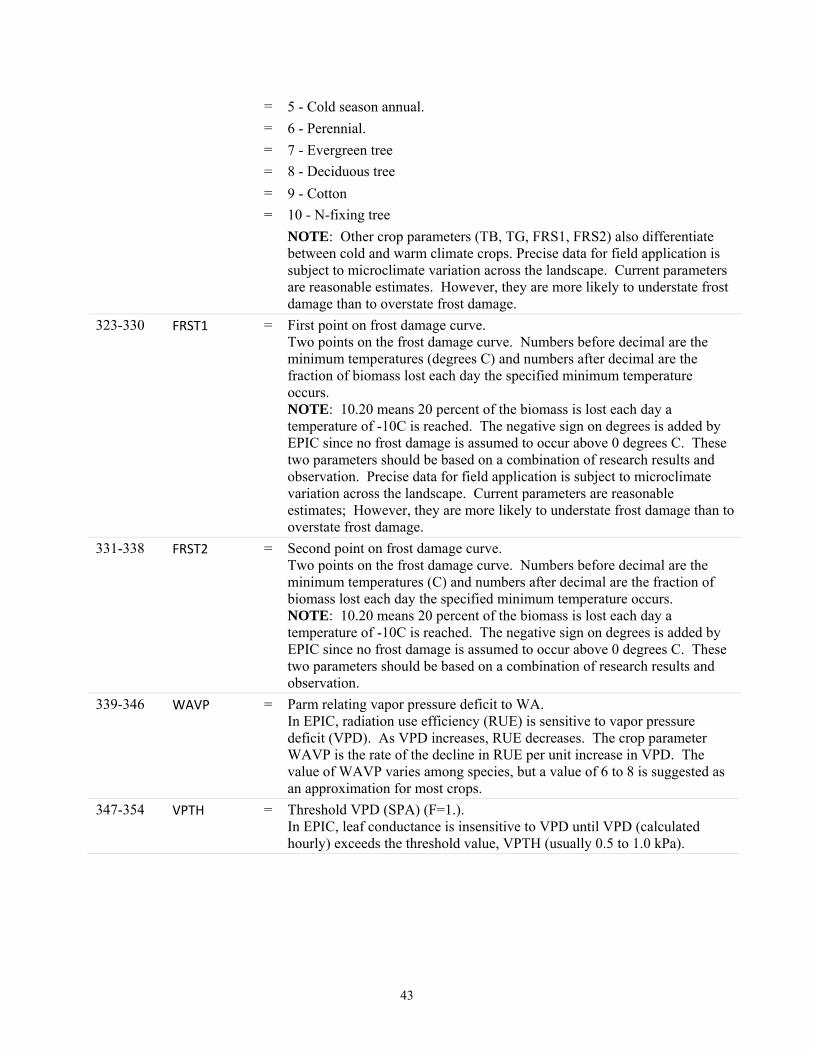
43

= 5 - Cold season annual.

= 6 - Perennial.

= 7 - Evergreen tree

= 8 - Deciduous tree

= 9 - Cotton

= 10 - N-fixing tree

NOTE: Other crop parameters (TB, TG, FRS1, FRS2) also differentiate between cold and warm climate crops. Precise data for field application is subject to microclimate variation across the landscape. Current parameters are reasonable estimates. However, they are more likely to understate frost damage than to overstate frost damage.

323-330 FRST1 = First point on frost damage curve. Two points on the frost damage curve. Numbers before decimal are the minimum temperatures (degrees C) and numbers after decimal are the fraction of biomass lost each day the specified minimum temperature occurs. NOTE: 10.20 means 20 percent of the biomass is lost each day a temperature of -10C is reached. The negative sign on degrees is added by EPIC since no frost damage is assumed to occur above 0 degrees C. These two parameters should be based on a combination of research results and observation. Precise data for field application is subject to microclimate variation across the landscape. Current parameters are reasonable estimates; However, they are more likely to understate frost damage than to overstate frost damage.

331-338 FRST2 = Second point on frost damage curve. Two points on the frost damage curve. Numbers before decimal are the minimum temperatures (C) and numbers after decimal are the fraction of biomass lost each day the specified minimum temperature occurs. NOTE: 10.20 means 20 percent of the biomass is lost each day a temperature of -10C is reached. The negative sign on degrees is added by EPIC since no frost damage is assumed to occur above 0 degrees C. These two parameters should be based on a combination of research results and observation.

339-346 WAVP = Parm relating vapor pressure deficit to WA. In EPIC, radiation use efficiency (RUE) is sensitive to vapor pressure deficit (VPD). As VPD increases, RUE decreases. The crop parameter WAVP is the rate of the decline in RUE per unit increase in VPD. The value of WAVP varies among species, but a value of 6 to 8 is suggested as an approximation for most crops.

347-354 VPTH = Threshold VPD (SPA) (F=1.). In EPIC, leaf conductance is insensitive to VPD until VPD (calculated hourly) exceeds the threshold value, VPTH (usually 0.5 to 1.0 kPa).

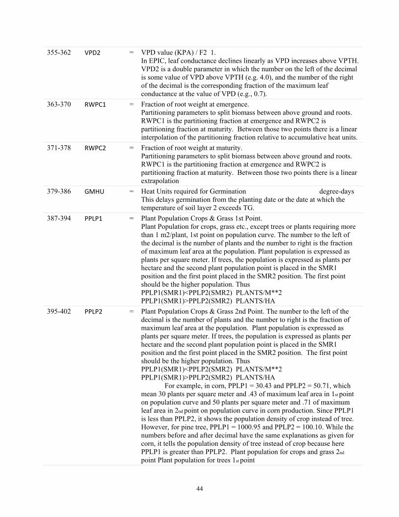
44

355-362 VPD2 = VPD value (KPA) / F2 1. In EPIC, leaf conductance declines linearly as VPD increases above VPTH. VPD2 is a double parameter in which the number on the left of the decimal is some value of VPD above VPTH (e.g. 4.0), and the number of the right of the decimal is the corresponding fraction of the maximum leaf conductance at the value of VPD (e.g., 0.7).

363-370 RWPC1 = Fraction of root weight at emergence. Partitioning parameters to split biomass between above ground and roots. RWPC1 is the partitioning fraction at emergence and RWPC2 is partitioning fraction at maturity. Between those two points there is a linear interpolation of the partitioning fraction relative to accumulative heat units.

371-378 RWPC2 = Fraction of root weight at maturity. Partitioning parameters to split biomass between above ground and roots. RWPC1 is the partitioning fraction at emergence and RWPC2 is partitioning fraction at maturity. Between those two points there is a linear extrapolation

379-386 GMHU = Heat Units required for Germination degree-days This delays germination from the planting date or the date at which the temperature of soil layer 2 exceeds TG.

387-394 PPLP1 = Plant Population Crops & Grass 1st Point. Plant Population for crops, grass etc., except trees or plants requiring more than 1 m2/plant, 1st point on population curve. The number to the left of the decimal is the number of plants and the number to right is the fraction of maximum leaf area at the population. Plant population is expressed as plants per square meter. If trees, the population is expressed as plants per hectare and the second plant population point is placed in the SMR1 position and the first point placed in the SMR2 position. The first point should be the higher population. Thus PPLP1(SMR1)<PPLP2(SMR2) PLANTS/M**2 PPLP1(SMR1)>PPLP2(SMR2) PLANTS/HA

395-402 PPLP2 = Plant Population Crops & Grass 2nd Point. The number to the left of the decimal is the number of plants and the number to right is the fraction of maximum leaf area at the population. Plant population is expressed as plants per square meter. If trees, the population is expressed as plants per hectare and the second plant population point is placed in the SMR1 position and the first point placed in the SMR2 position. The first point should be the higher population. Thus PPLP1(SMR1)<PPLP2(SMR2) PLANTS/M**2 PPLP1(SMR1)>PPLP2(SMR2) PLANTS/HA For example, in corn, PPLP1 = 30.43 and PPLP2 = 50.71, which mean 30 plants per square meter and .43 of maximum leaf area in 1st point on population curve and 50 plants per square meter and .71 of maximum leaf area in 2nd point on population curve in corn production. Since PPLP1 is less than PPLP2, it shows the population density of crop instead of tree. However, for pine tree, PPLP1 = 1000.95 and PPLP2 = 100.10. While the numbers before and after decimal have the same explanations as given for corn, it tells the population density of tree instead of crop because here PPLP1 is greater than PPLP2. Plant population for crops and grass 2nd

point Plant population for trees 1st point

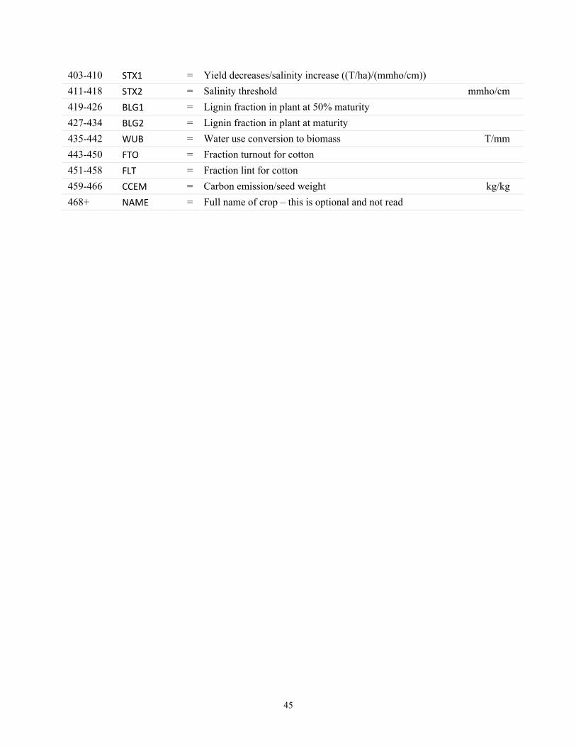
45

403-410 STX1 = Yield decreases/salinity increase ((T/ha)/(mmho/cm))

411-418 STX2 = Salinity threshold mmho/cm

419-426 BLG1 = Lignin fraction in plant at 50% maturity

427-434 BLG2 = Lignin fraction in plant at maturity

435-442 WUB = Water use conversion to biomass T/mm

443-450 FTO = Fraction turnout for cotton

451-458 FLT = Fraction lint for cotton

459-466 CCEM = Carbon emission/seed weight kg/kg

468+ NAME = Full name of crop – this is optional and not read

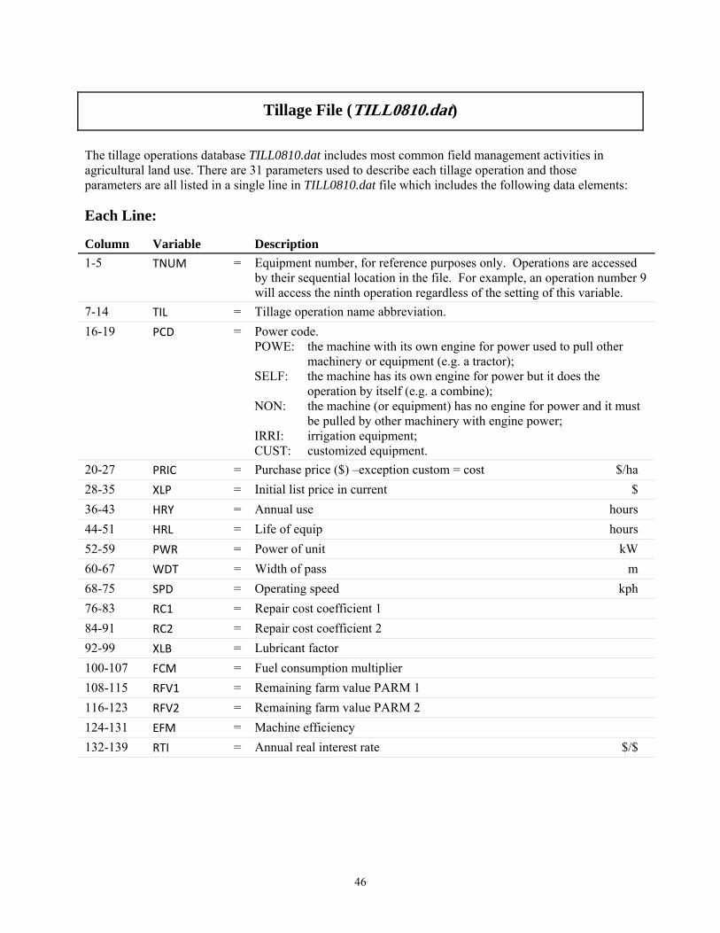
46

Tillage File (TILL0810.dat)

The tillage operations database TILL0810.dat includes most common field management activities in agricultural land use. There are 31 parameters used to describe each tillage operation and those parameters are all listed in a single line in TILL0810.dat file which includes the following data elements:

Each Line:


1-5 TNUM = Equipment number, for reference purposes only. Operations are accessed by their sequential location in the file. For example, an operation number 9 will access the ninth operation regardless of the setting of this variable.

7-14 TIL = Tillage operation name abbreviation.

16-19 PCD = Power code. POWE: the machine with its own engine for power used to pull other

machinery or equipment (e.g. a tractor); SELF: the machine has its own engine for power but it does the

operation by itself (e.g. a combine); NON: the machine (or equipment) has no engine for power and it must

be pulled by other machinery with engine power; IRRI: irrigation equipment; CUST: customized equipment.

20-27 PRIC = Purchase price ($) –exception custom = cost $/ha

28-35 XLP = Initial list price in current $

36-43 HRY = Annual use hours

44-51 HRL = Life of equip hours

52-59 PWR = Power of unit kW

60-67 WDT = Width of pass m

68-75 SPD = Operating speed kph

76-83 RC1 = Repair cost coefficient 1

84-91 RC2 = Repair cost coefficient 2

92-99 XLB = Lubricant factor

100-107 FCM = Fuel consumption multiplier

108-115 RFV1 = Remaining farm value PARM 1

116-123 RFV2 = Remaining farm value PARM 2

124-131 EFM = Machine efficiency

132-139 RTI = Annual real interest rate $/$

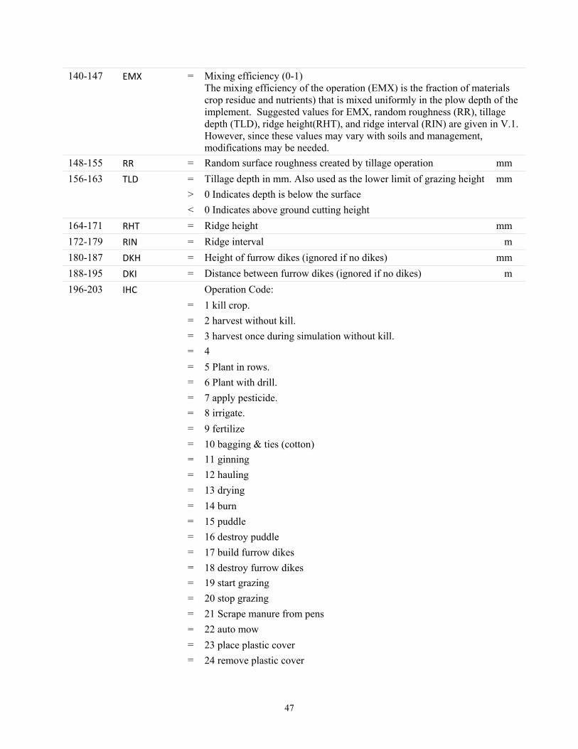
47

140-147 EMX = Mixing efficiency (0-1) The mixing efficiency of the operation (EMX) is the fraction of materials crop residue and nutrients) that is mixed uniformly in the plow depth of the implement. Suggested values for EMX, random roughness (RR), tillage depth (TLD), ridge height(RHT), and ridge interval (RIN) are given in V.1. However, since these values may vary with soils and management, modifications may be needed.

148-155 RR = Random surface roughness created by tillage operation mm

156-163 TLD = Tillage depth in mm. Also used as the lower limit of grazing height mm

> 0 Indicates depth is below the surface

< 0 Indicates above ground cutting height

164-171 RHT = Ridge height mm

172-179 RIN = Ridge interval m

180-187 DKH = Height of furrow dikes (ignored if no dikes) mm

188-195 DKI = Distance between furrow dikes (ignored if no dikes) m

196-203 IHC Operation Code:

= 1 kill crop.

= 2 harvest without kill.

= 3 harvest once during simulation without kill.

= 4

= 5 Plant in rows.

= 6 Plant with drill.

= 7 apply pesticide.

= 8 irrigate.

= 9 fertilize

= 10 bagging & ties (cotton)

= 11 ginning

= 12 hauling

= 13 drying

= 14 burn

= 15 puddle

= 16 destroy puddle

= 17 build furrow dikes

= 18 destroy furrow dikes

= 19 start grazing

= 20 stop grazing

= 21 Scrape manure from pens

= 22 auto mow

= 23 place plastic cover

= 24 remove plastic cover

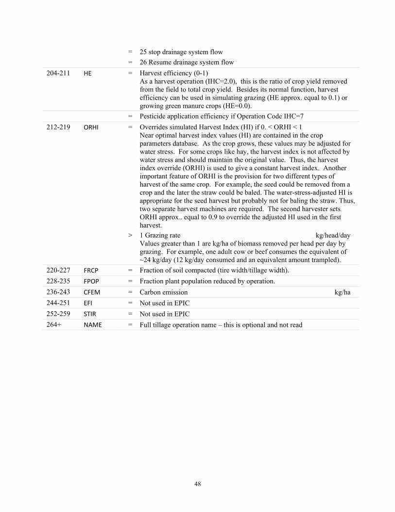
48

= 25 stop drainage system flow

= 26 Resume drainage system flow

204-211 HE = Harvest efficiency (0-1) As a harvest operation (IHC=2.0), this is the ratio of crop yield removed from the field to total crop yield. Besides its normal function, harvest efficiency can be used in simulating grazing (HE approx. equal to 0.1) or growing green manure crops (HE=0.0).

= Pesticide application efficiency if Operation Code IHC=7

212-219 ORHI = Overrides simulated Harvest Index (HI) if 0. < ORHI < 1 Near optimal harvest index values (HI) are contained in the crop parameters database. As the crop grows, these values may be adjusted for water stress. For some crops like hay, the harvest index is not affected by water stress and should maintain the original value. Thus, the harvest index override (ORHI) is used to give a constant harvest index. Another important feature of ORHI is the provision for two different types of harvest of the same crop. For example, the seed could be removed from a crop and the later the straw could be baled. The water-stress-adjusted HI is appropriate for the seed harvest but probably not for baling the straw. Thus, two separate harvest machines are required. The second harvester sets ORHI approx.. equal to 0.9 to override the adjusted HI used in the first harvest.

> 1 Grazing rate kg/head/day Values greater than 1 are kg/ha of biomass removed per head per day by grazing. For example, one adult cow or beef consumes the equivalent of ~24 kg/day (12 kg/day consumed and an equivalent amount trampled).

220-227 FRCP = Fraction of soil compacted (tire width/tillage width).

228-235 FPOP = Fraction plant population reduced by operation.

236-243 CFEM = Carbon emission kg/ha

244-251 EFI = Not used in EPIC

252-259 STIR = Not used in EPIC

264+ NAME = Full tillage operation name – this is optional and not read

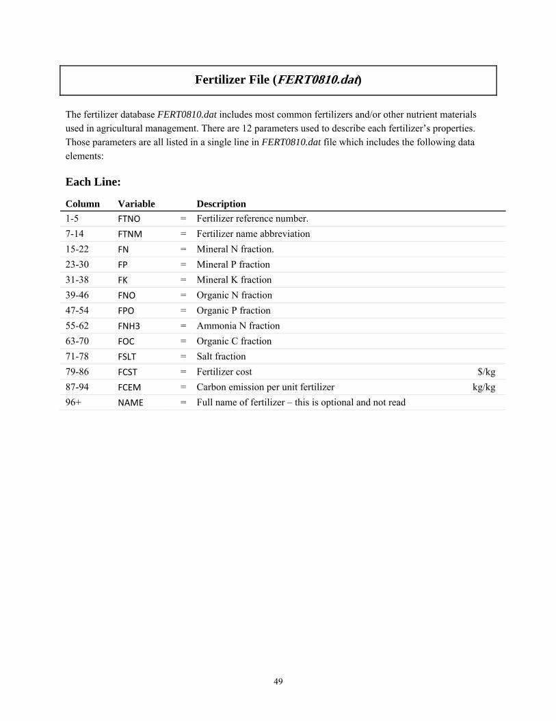
49

Fertilizer File (FERT0810.dat)

The fertilizer database FERT0810.dat includes most common fertilizers and/or other nutrient materials used in agricultural management. There are 12 parameters used to describe each fertilizer’s properties. Those parameters are all listed in a single line in FERT0810.dat file which includes the following data elements:

Each Line:


1-5 FTNO = Fertilizer reference number.

7-14 FTNM = Fertilizer name abbreviation

15-22 FN = Mineral N fraction.

23-30 FP = Mineral P fraction

31-38 FK = Mineral K fraction

39-46 FNO = Organic N fraction

47-54 FPO = Organic P fraction

55-62 FNH3 = Ammonia N fraction

63-70 FOC = Organic C fraction

71-78 FSLT = Salt fraction

79-86 FCST = Fertilizer cost $/kg

87-94 FCEM = Carbon emission per unit fertilizer kg/kg

96+ NAME = Full name of fertilizer – this is optional and not read

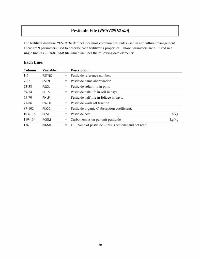
50

Pesticide File (PEST0810.dat)

The fertilizer database PEST0810.dat includes most common pesticides used in agricultural management. There are 9 parameters used to describe each fertilizer’s properties. Those parameters are all listed in a single line in PEST0810.dat file which includes the following data elements:

Each Line:


1-5 PSTNO = Pesticide reference number.

7-22 PSTN = Pesticide name abbreviation

23-38 PSOL = Pesticide solubility in ppm.

39-54 PHLS = Pesticide half-life in soil in days.

55-70 PHLF = Pesticide half-life in foliage in days.

71-86 PWOF = Pesticide wash off fraction.

87-102 PKOC = Pesticide organic C absorption coefficient.

103-118 PCST = Pesticide cost $/kg

119-134 PCEM = Carbon emission per unit pesticide kg/kg

136+ NAME = Full name of pesticide – this is optional and not read

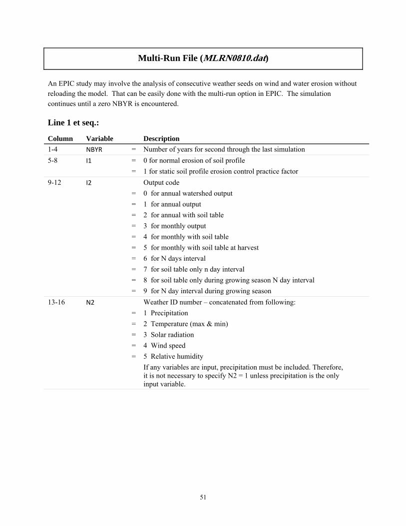
51

Multi-Run File (MLRN0810.dat)

An EPIC study may involve the analysis of consecutive weather seeds on wind and water erosion without reloading the model. That can be easily done with the multi-run option in EPIC. The simulation continues until a zero NBYR is encountered.

Line 1 et seq.:


1-4 NBYR = Number of years for second through the last simulation

5-8 I1 = 0 for normal erosion of soil profile

= 1 for static soil profile erosion control practice factor

9-12 I2 Output code

= 0 for annual watershed output

= 1 for annual output

= 2 for annual with soil table

= 3 for monthly output

= 4 for monthly with soil table

= 5 for monthly with soil table at harvest

= 6 for N days interval

= 7 for soil table only n day interval

= 8 for soil table only during growing season N day interval

= 9 for N day interval during growing season

13-16 N2 Weather ID number – concatenated from following:

= 1 Precipitation

= 2 Temperature (max & min)

= 3 Solar radiation

= 4 Wind speed

= 5 Relative humidity

If any variables are input, precipitation must be included. Therefore, it is not necessary to specify N2 = 1 unless precipitation is the only input variable.

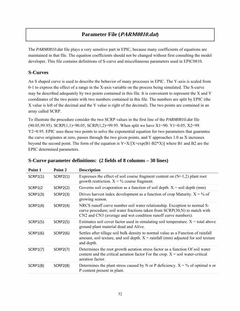
52

Parameter File (PARM0810.dat)

The PARM0810.dat file plays a very sensitive part in EPIC, because many coefficients of equations are maintained in that file. The equation coefficients should not be changed without first consulting the model developer. This file contains definitions of S-curve and miscellaneous parameters used in EPIC0810.

S-Curves

An S shaped curve is used to describe the behavior of many processes in EPIC. The Y-axis is scaled from 0-1 to express the effect of a range in the X-axis variable on the process being simulated. The S-curve may be described adequately by two points contained in this file. It is convenient to represent the X and Y coordinates of the two points with two numbers contained in this file. The numbers are split by EPIC (the X value is left of the decimal and the Y value is right of the decimal). The two points are contained in an array called SCRP.

To illustrate the procedure consider the two SCRP values in the first line of the PARM0810.dat file (90.05,99.95). SCRP(1,1)=90.05, SCRP(1,2)=99.95. When split we have X1=90. Y1=0.05; X2=99. Y2=0.95. EPIC uses these two points to solve the exponential equation for two parameters that guarantee the curve originates at zero, passes through the two given points, and Y approaches 1.0 as X increases beyond the second point. The form of the equation is Y=X/[X+exp(B1-B2*X)] where B1 and B2 are the EPIC determined parameters.

S-Curve parameter definitions: (2 fields of 8 columns – 30 lines)

Point 1 Point 2 Description

SCRP1(1) SCRP2(1) Expresses the effect of soil course fragment content on (N=1,2) plant root growth restriction. X = % course fragment.

SCRP1(2 SCRP2(2) Governs soil evaporation as a function of soil depth. X = soil depth (mm)

SCRP1(3) SCRP2(3) Drives harvest index development as a function of crop Maturity. X = % of growing season.

SCRP1(4) SCRP2(4) NRCS runoff curve number soil water relationship. Exception to normal S-curve procedure; soil water fractions taken from SCRP(30,N) to match with CN2 and CN3 (average and wet condition runoff curve numbers).

SCRP1(5) SCRP2(5) Estimates soil cover factor used in simulating soil temperature. X = total above ground plant material dead and Alive.

SCRP1(6) SCRP2(6) Settles after tillage soil bulk density to normal value as a Function of rainfall amount, soil texture, and soil depth. X = rainfall (mm) adjusted for soil texture and depth.

SCRP1(7) SCRP2(7) Determines the root growth aeration stress factor as a function Of soil water content and the critical aeration factor For the crop. X = soil water-critical aeration factor.

SCRP1(8) SCRP2(8) Determines the plant stress caused by N or P deficiency. X = % of optimal n or P content present in plant.

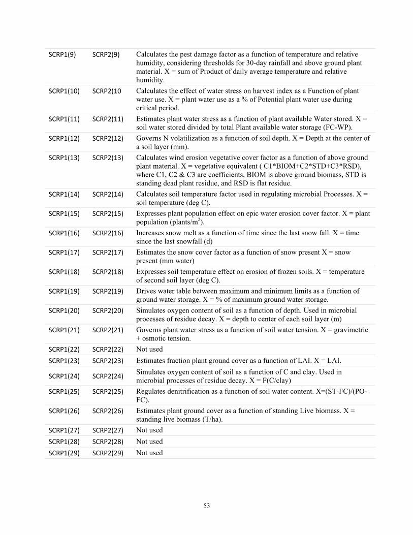
53

SCRP1(9) SCRP2(9) Calculates the pest damage factor as a function of temperature and relative humidity, considering thresholds for 30-day rainfall and above ground plant material. X = sum of Product of daily average temperature and relative humidity.

SCRP1(10) SCRP2(10 Calculates the effect of water stress on harvest index as a Function of plant water use. X = plant water use as a % of Potential plant water use during critical period.

SCRP1(11) SCRP2(11) Estimates plant water stress as a function of plant available Water stored. X = soil water stored divided by total Plant available water storage (FC-WP).

SCRP1(12) SCRP2(12) Governs N volatilization as a function of soil depth. X = Depth at the center of a soil layer (mm).

SCRP1(13) SCRP2(13) Calculates wind erosion vegetative cover factor as a function of above ground plant material. X = vegetative equivalent ( C1*BIOM+C2*STD+C3*RSD), where C1, C2 & C3 are coefficients, BIOM is above ground biomass, STD is standing dead plant residue, and RSD is flat residue.

SCRP1(14) SCRP2(14) Calculates soil temperature factor used in regulating microbial Processes. X = soil temperature (deg C).

SCRP1(15) SCRP2(15) Expresses plant population effect on epic water erosion cover factor. X = plant population (plants/m2).

SCRP1(16) SCRP2(16) Increases snow melt as a function of time since the last snow fall. X = time since the last snowfall (d)

SCRP1(17) SCRP2(17) Estimates the snow cover factor as a function of snow present X = snow present (mm water)

SCRP1(18) SCRP2(18) Expresses soil temperature effect on erosion of frozen soils. X = temperature of second soil layer (deg C).

SCRP1(19) SCRP2(19) Drives water table between maximum and minimum limits as a function of ground water storage. X = % of maximum ground water storage.

SCRP1(20) SCRP2(20) Simulates oxygen content of soil as a function of depth. Used in microbial processes of residue decay. X = depth to center of each soil layer (m)

SCRP1(21) SCRP2(21) Governs plant water stress as a function of soil water tension. X = gravimetric + osmotic tension.

SCRP1(22) SCRP2(22) Not used

SCRP1(23) SCRP2(23) Estimates fraction plant ground cover as a function of LAI. X = LAI.

SCRP1(24) SCRP2(24) Simulates oxygen content of soil as a function of C and clay. Used in microbial processes of residue decay. X = F(C/clay)

SCRP1(25) SCRP2(25) Regulates denitrification as a function of soil water content. X=(ST-FC)/(PO-FC).

SCRP1(26) SCRP2(26) Estimates plant ground cover as a function of standing Live biomass. X = standing live biomass (T/ha).




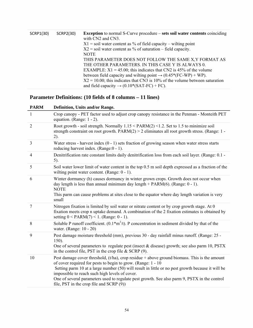
54

SCRP1(30) SCRP2(30) Exception to normal S-Curve procedure – sets soil water contents coinciding with CN2 and CN3. X1 = soil water content as % of field capacity – wilting point X2 = soil water content as % of saturation – field capacity. NOTE THIS PARAMETER DOES NOT FOLLOW THE SAME X,Y FORMAT AS THE OTHER PARAMETERS. IN THIS CASE Y IS ALWAYS 0. EXAMPLE: X1 = 45.00; this indicates that CN2 is 45% of the volume between field capacity and wilting point → (0.45*(FC-WP) + WP). X2 = 10.00; this indicates that CN3 is 10% of the volume between saturation and field capacity → (0.10*(SAT-FC) + FC).

Parameter Definitions: (10 fields of 8 columns – 11 lines)

PARM Definition, Units and/or Range.

1 Crop canopy - PET factor used to adjust crop canopy resistance in the Penman - Monteith PET equation. (Range: 1 - 2).

2 Root growth - soil strength. Normally 1.15 < PARM(2) <1.2. Set to 1.5 to minimize soil strength constraint on root growth. PARM(2) > 2 eliminates all root growth stress. (Range: 1 - 2).

3 Water stress - harvest index (0 - 1) sets fraction of growing season when water stress starts reducing harvest index. (Range:0 - 1).

4 Denitrification rate constant limits daily denitrification loss from each soil layer. (Range: 0.1 - 5).

5 Soil water lower limit of water content in the top 0.5 m soil depth expressed as a fraction of the wilting point water content. (Range: 0 - 1).

6 Winter dormancy (h) causes dormancy in winter grown crops. Growth does not occur when day length is less than annual minimum day length + PARM(6). (Range: 0 - 1). NOTE This parm can cause problems at sites close to the equator where day length variation is very small

7 Nitrogen fixation is limited by soil water or nitrate content or by crop growth stage. At 0 fixation meets crop n uptake demand. A combination of the 2 fixation estimates is obtained by setting 0 < PARM(7) < 1. (Range: 0 - 1).

8 Soluble P runoff coefficient. (0.1*m3/t). P concentration in sediment divided by that of the water. (Range: 10 - 20)

9 Pest damage moisture threshold (mm), previous 30 - day rainfall minus runoff. (Range: 25 - 150). One of several parameters to regulate pest (insect & disease) growth; see also parm 10, PSTX in the control file, PST in the crop file & SCRP (9).

10 Pest damage cover threshold, (t/ha), crop residue + above ground biomass. This is the amount of cover required for pests to begin to grow. (Range: 1 - 10 Setting parm 10 at a large number (50) will result in little or no pest growth because it will be impossible to reach such high levels of cover. One of several parameters used to regulate pest growth. See also parm 9, PSTX in the control file, PST in the crop file and SCRP (9))

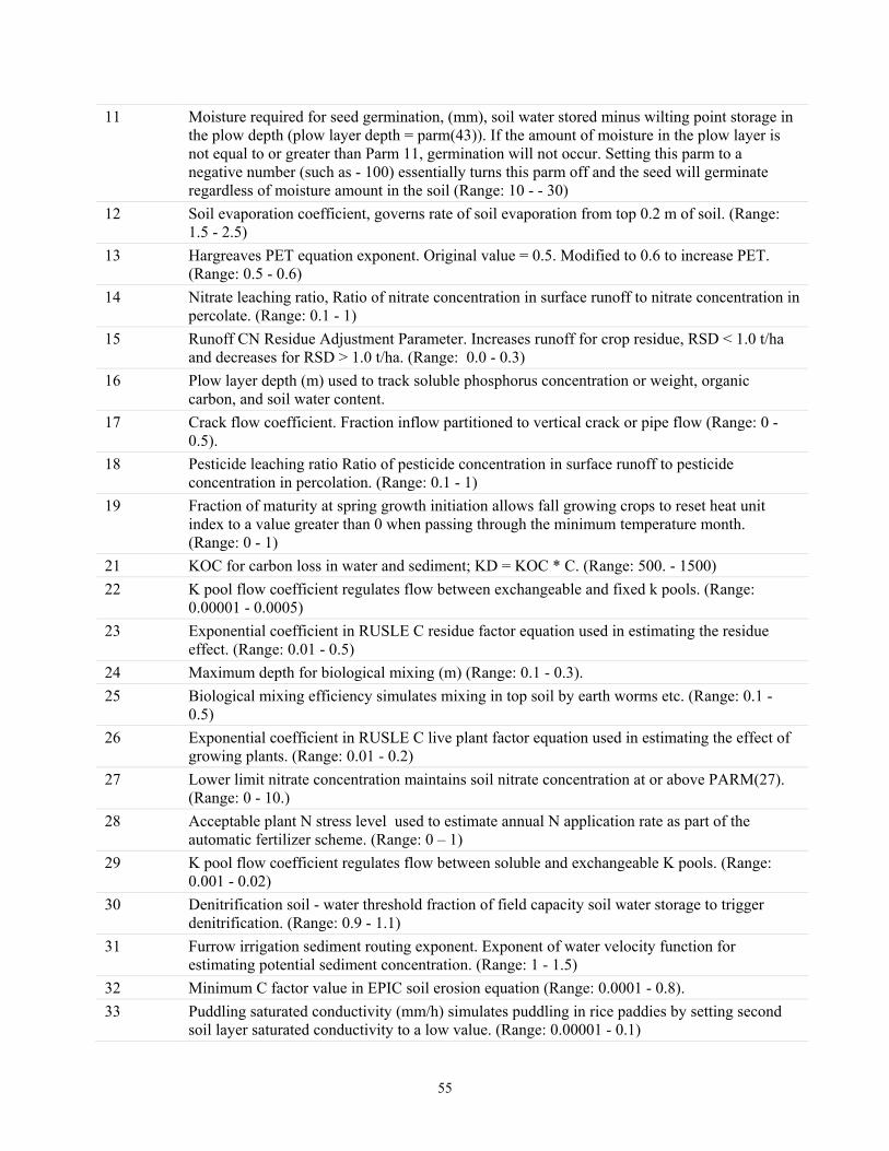
55

11 Moisture required for seed germination, (mm), soil water stored minus wilting point storage in the plow depth (plow layer depth = parm(43)). If the amount of moisture in the plow layer is not equal to or greater than Parm 11, germination will not occur. Setting this parm to a negative number (such as - 100) essentially turns this parm off and the seed will germinate regardless of moisture amount in the soil (Range: 10 - - 30)

12 Soil evaporation coefficient, governs rate of soil evaporation from top 0.2 m of soil. (Range: 1.5 - 2.5)

13 Hargreaves PET equation exponent. Original value = 0.5. Modified to 0.6 to increase PET. (Range: 0.5 - 0.6)

14 Nitrate leaching ratio, Ratio of nitrate concentration in surface runoff to nitrate concentration in percolate. (Range: 0.1 - 1)

15 Runoff CN Residue Adjustment Parameter. Increases runoff for crop residue, RSD < 1.0 t/ha and decreases for RSD > 1.0 t/ha. (Range: 0.0 - 0.3)

16 Plow layer depth (m) used to track soluble phosphorus concentration or weight, organic carbon, and soil water content.

17 Crack flow coefficient. Fraction inflow partitioned to vertical crack or pipe flow (Range: 0 - 0.5).

18 Pesticide leaching ratio Ratio of pesticide concentration in surface runoff to pesticide concentration in percolation. (Range: 0.1 - 1)

19 Fraction of maturity at spring growth initiation allows fall growing crops to reset heat unit index to a value greater than 0 when passing through the minimum temperature month. (Range: 0 - 1)

21 KOC for carbon loss in water and sediment; KD = KOC * C. (Range: 500. - 1500)

22 K pool flow coefficient regulates flow between exchangeable and fixed k pools. (Range: 0.00001 - 0.0005)

23 Exponential coefficient in RUSLE C residue factor equation used in estimating the residue effect. (Range: 0.01 - 0.5)

24 Maximum depth for biological mixing (m) (Range: 0.1 - 0.3).

25 Biological mixing efficiency simulates mixing in top soil by earth worms etc. (Range: 0.1 - 0.5)

26 Exponential coefficient in RUSLE C live plant factor equation used in estimating the effect of growing plants. (Range: 0.01 - 0.2)

27 Lower limit nitrate concentration maintains soil nitrate concentration at or above PARM(27). (Range: 0 - 10.)

28 Acceptable plant N stress level used to estimate annual N application rate as part of the automatic fertilizer scheme. (Range: 0 – 1)

29 K pool flow coefficient regulates flow between soluble and exchangeable K pools. (Range: 0.001 - 0.02)

30 Denitrification soil - water threshold fraction of field capacity soil water storage to trigger denitrification. (Range: 0.9 - 1.1)

31 Furrow irrigation sediment routing exponent. Exponent of water velocity function for estimating potential sediment concentration. (Range: 1 - 1.5)

32 Minimum C factor value in EPIC soil erosion equation (Range: 0.0001 - 0.8).

33 Puddling saturated conductivity (mm/h) simulates puddling in rice paddies by setting second soil layer saturated conductivity to a low value. (Range: 0.00001 - 0.1)

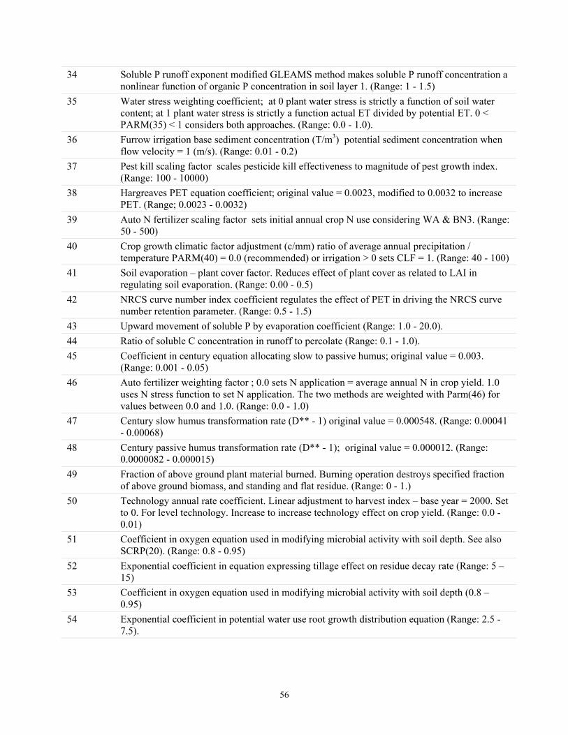
56

34 Soluble P runoff exponent modified GLEAMS method makes soluble P runoff concentration a nonlinear function of organic P concentration in soil layer 1. (Range: 1 - 1.5)

35 Water stress weighting coefficient; at 0 plant water stress is strictly a function of soil water content; at 1 plant water stress is strictly a function actual ET divided by potential ET. 0 < PARM(35) < 1 considers both approaches. (Range: 0.0 - 1.0).

36 Furrow irrigation base sediment concentration (T/m3) potential sediment concentration when flow velocity = 1 (m/s). (Range: 0.01 - 0.2)

37 Pest kill scaling factor scales pesticide kill effectiveness to magnitude of pest growth index. (Range: 100 - 10000)

38 Hargreaves PET equation coefficient; original value = 0.0023, modified to 0.0032 to increase PET. (Range; 0.0023 - 0.0032)

39 Auto N fertilizer scaling factor sets initial annual crop N use considering WA & BN3. (Range: 50 - 500)

40 Crop growth climatic factor adjustment (c/mm) ratio of average annual precipitation / temperature PARM(40) = 0.0 (recommended) or irrigation > 0 sets CLF = 1. (Range: 40 - 100)

41 Soil evaporation – plant cover factor. Reduces effect of plant cover as related to LAI in regulating soil evaporation. (Range: 0.00 - 0.5)

42 NRCS curve number index coefficient regulates the effect of PET in driving the NRCS curve number retention parameter. (Range: 0.5 - 1.5)

43 Upward movement of soluble P by evaporation coefficient (Range: 1.0 - 20.0).

44 Ratio of soluble C concentration in runoff to percolate (Range: 0.1 - 1.0).

45 Coefficient in century equation allocating slow to passive humus; original value = 0.003. (Range: 0.001 - 0.05)

46 Auto fertilizer weighting factor ; 0.0 sets N application = average annual N in crop yield. 1.0 uses N stress function to set N application. The two methods are weighted with Parm(46) for values between 0.0 and 1.0. (Range: 0.0 - 1.0)

47 Century slow humus transformation rate (D** - 1) original value = 0.000548. (Range: 0.00041 - 0.00068)

48 Century passive humus transformation rate (D** - 1); original value = 0.000012. (Range: 0.0000082 - 0.000015)

49 Fraction of above ground plant material burned. Burning operation destroys specified fraction of above ground biomass, and standing and flat residue. (Range: 0 - 1.)

50 Technology annual rate coefficient. Linear adjustment to harvest index – base year = 2000. Set to 0. For level technology. Increase to increase technology effect on crop yield. (Range: 0.0 - 0.01)

51 Coefficient in oxygen equation used in modifying microbial activity with soil depth. See also SCRP(20). (Range: 0.8 - 0.95)

52 Exponential coefficient in equation expressing tillage effect on residue decay rate (Range: 5 – 15)

53 Coefficient in oxygen equation used in modifying microbial activity with soil depth (0.8 – 0.95)

54 Exponential coefficient in potential water use root growth distribution equation (Range: 2.5 - 7.5).

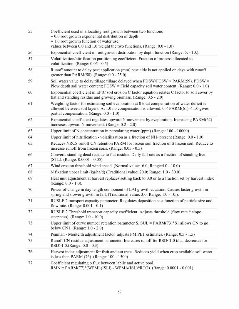
57

55 Coefficient used in allocating root growth between two functions = 0.0 root growth exponential distribution of depth = 1.0 root growth function of water use; values between 0.0 and 1.0 weight the two functions. (Range: 0.0 - 1.0)

56 Exponential coefficient in root growth distribution by depth function (Range: 5. - 10.).

57 Volatilization/nitrification partitioning coefficient. Fraction of process allocated to volatilization. (Range: 0.05 - 0.5)

58 Runoff amount to delay pest application (mm) pesticide is not applied on days with runoff greater than PARM(58). (Range: 0.0 - 25.0)

59 Soil water value to delay tillage tillage delayed when PDSW/FCSW > PARM(59). PDSW = Plow depth soil water content; FCSW = Field capacity soil water content. (Range: 0.0 - 1.0)

60 Exponential coefficient in EPIC soil erosion C factor equation relates C factor to soil cover by flat and standing residue and growing biomass. (Range: 0.5 - 2.0)

61 Weighting factor for estimating soil evaporation at 0 total compensation of water deficit is allowed between soil layers. At 1.0 no compensation is allowed. 0 < PARM(61) < 1.0 gives partial compensation. (Range: 0.0 - 1.0)

62 Exponential coefficient regulates upward N movement by evaporation. Increasing PARM(62) increases upward N movement. (Range: 0.2 - 2.0)

63 Upper limit of N concentration in percolating water (ppm) (Range: 100 - 10000).

64 Upper limit of nitrification - volatilization as a fraction of NH3 present (Range: 0.0 - 1.0).

65 Reduces NRCS runoff CN retention PARM for frozen soil fraction of S frozen soil. Reduce to increase runoff from frozen soils. (Range: 0.05 - 0.5)

66 Converts standing dead residue to flat residue. Daily fall rate as a fraction of standing live (STL). (Range: 0.0001 - 0.05).

67 Wind erosion threshold wind speed. (Normal value: 6.0; Range:4.0 - 10.0).

68 N fixation upper limit (kg/ha/d) (Traditional value: 20.0; Range: 1.0 - 30.0).

69 Heat unit adjustment at harvest replaces setting back to 0.0 or to a fraction set by harvest index (Range: 0.0 - 1.0).

70 Power of change in day length component of LAI growth equation. Causes faster growth in spring and slower growth in fall. (Traditional value: 3.0; Range: 1.0 - 10.).

71 RUSLE 2 transport capacity parameter. Regulates deposition as a function of particle size and flow rate. (Range: 0.001 - 0.1)

72 RUSLE 2 Threshold transport capacity coefficient. Adjusts threshold (flow rate * slope steepness). (Range: 1.0 - 10.0)

73 Upper limit of curve number retention parameter S. SUL = PARM(73)*S1 allows CN to go below CN1. (Range: 1.0 - 2.0)

74 Penman - Monteith adjustment factor adjusts PM PET estimates. (Range: 0.5 - 1.5)

75 Runoff CN residue adjustment parameter. Increases runoff for RSD<1.0 t/ha; decreases for RSD>1.0.(Range: 0.0 - 0.3)

76 Harvest index adjustment for fruit and nut trees. Reduces yield when crop available soil water is less than PARM (76). (Range: 100 - 1500)

77 Coefficient regulating p flux between labile and active pool. RMN = PARM(77)*(WPML(ISLl) - WPMA(ISL)*RTO). (Range: 0.0001 - 0.001)

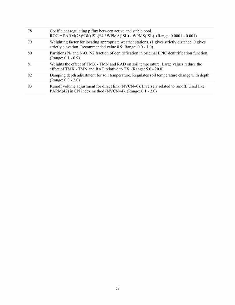
58

78 Coefficient regulating p flux between active and stable pool. ROC = PARM(78)*BK(ISL)*4.*WPMA(ISL) - WPMS(ISL). (Range: 0.0001 - 0.001)

79 Weighting factor for locating appropriate weather stations. (1 gives strictly distance; 0 gives strictly elevation. Recommended value 0.9; Range: 0.0 - 1.0)

80 Partitions N2 and N2O. N2 fraction of denitrification in original EPIC denitrification function. (Range: 0.1 - 0.9)

81 Weights the effect of TMX - TMN and RAD on soil temperature. Large values reduce the effect of TMX - TMN and RAD relative to TX. (Range: 5.0 - 20.0)

82 Damping depth adjustment for soil temperature. Regulates soil temperature change with depth (Range: 0.0 - 2.0)

83 Runoff volume adjustment for direct link (NVCN=0). Inversely related to runoff. Used like PARM(42) in CN index method (NVCN=4). (Range: 0.1 - 2.0)

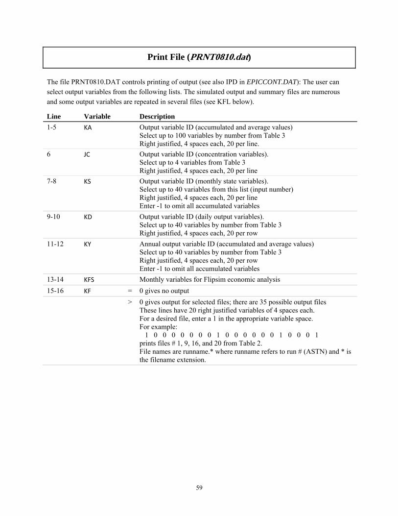
59

Print File (PRNT0810.dat)

The file PRNT0810.DAT controls printing of output (see also IPD in EPICCONT.DAT): The user can select output variables from the following lists. The simulated output and summary files are numerous and some output variables are repeated in several files (see KFL below).


1-5 KA Output variable ID (accumulated and average values) Select up to 100 variables by number from Table 3 Right justified, 4 spaces each, 20 per line.

6 JC Output variable ID (concentration variables). Select up to 4 variables from Table 3 Right justified, 4 spaces each, 20 per line

7-8 KS Output variable ID (monthly state variables). Select up to 40 variables from this list (input number) Right justified, 4 spaces each, 20 per line Enter -1 to omit all accumulated variables

9-10 KD Output variable ID (daily output variables). Select up to 40 variables by number from Table 3 Right justified, 4 spaces each, 20 per row

11-12 KY Annual output variable ID (accumulated and average values) Select up to 40 variables by number from Table 3 Right justified, 4 spaces each, 20 per row Enter -1 to omit all accumulated variables

13-14 KFS Monthly variables for Flipsim economic analysis

15-16 KF = 0 gives no output

> 0 gives output for selected files; there are 35 possible output files These lines have 20 right justified variables of 4 spaces each. For a desired file, enter a 1 in the appropriate variable space. For example: 1 0 0 0 0 0 0 0 1 0 0 0 0 0 0 1 0 0 0 1 prints files # 1, 9, 16, and 20 from Table 2. File names are runname.* where runname refers to run # (ASTN) and * is the filename extension.

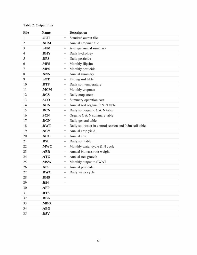
60

Table 2: Output Files

File Name Description

1 .OUT = Standard output file

2 .ACM = Annual cropman file

3 .SUM = Average annual summary

4 .DHY = Daily hydrology

5 .DPS = Daily pesticide

6 .MFS = Monthly flipsim

7 .MPS = Monthly pesticide

8 .ANN = Annual summary

9 .SOT = Ending soil table

10 .DTP = Daily soil temperature

11 .MCM = Monthly cropman

12 .DCS = Daily crop stress

13 .SCO = Summary operation cost

14 .ACN = Annual soil organic C & N table

15 .DCN = Daily soil organic C & N table

16 .SCN = Organic C & N summary table

17 .DGN = Daily general table

18 .DWT = Daily soil water in control section and 0.5m soil table

19 .ACY = Annual crop yield

20 .ACO = Annual cost

21 .DSL = Daily soil table

22 .MWC = Monthly water cycle & N cycle

23 .ABR = Annual biomass root weight

24 .ATG = Annual tree growth

25 .MSW = Monthly output to SWAT

26 .APS = Annual pesticide

27 .DWC = Daily water cycle

28 .DHS =

29 .R84 =

30 .APP

31 .RTS

32 .DBG

33 .MBG

34 .ABG

35 .DSV

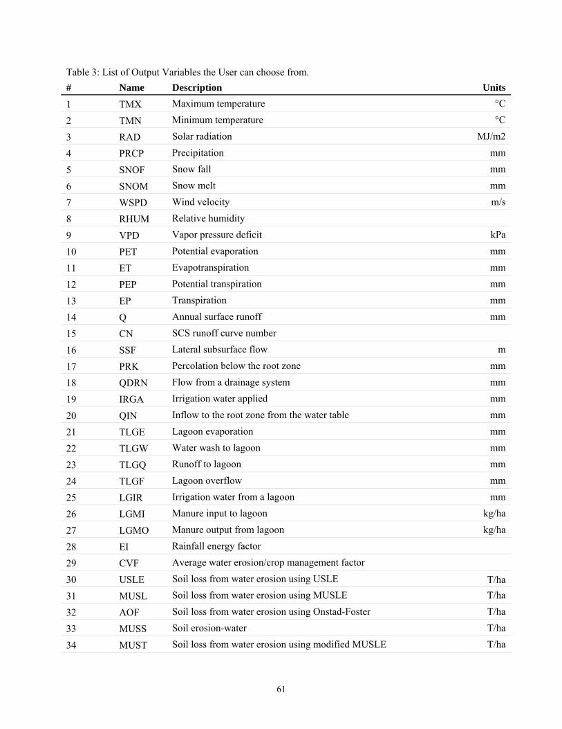
61

Table 3: List of Output Variables the User can choose from.

# Name Description Units

1 TMX Maximum temperature °C

2 TMN Minimum temperature °C

3 RAD Solar radiation MJ/m2

4 PRCP Precipitation mm

5 SNOF Snow fall mm

6 SNOM Snow melt mm

7 WSPD Wind velocity m/s

8 RHUM Relative humidity

9 VPD Vapor pressure deficit kPa

10 PET Potential evaporation mm

11 ET Evapotranspiration mm

12 PEP Potential transpiration mm

13 EP Transpiration mm

14 Q Annual surface runoff mm

15 CN SCS runoff curve number

16 SSF Lateral subsurface flow m

17 PRK Percolation below the root zone mm

18 QDRN Flow from a drainage system mm

19 IRGA Irrigation water applied mm

20 QIN Inflow to the root zone from the water table mm

21 TLGE Lagoon evaporation mm

22 TLGW Water wash to lagoon mm

23 TLGQ Runoff to lagoon mm

24 TLGF Lagoon overflow mm

25 LGIR Irrigation water from a lagoon mm

26 LGMI Manure input to lagoon kg/ha

27 LGMO Manure output from lagoon kg/ha

28 EI Rainfall energy factor

29 CVF Average water erosion/crop management factor

30 USLE Soil loss from water erosion using USLE T/ha

31 MUSL Soil loss from water erosion using MUSLE T/ha

32 AOF Soil loss from water erosion using Onstad-Foster T/ha

33 MUSS Soil erosion-water T/ha

34 MUST Soil loss from water erosion using modified MUSLE T/ha

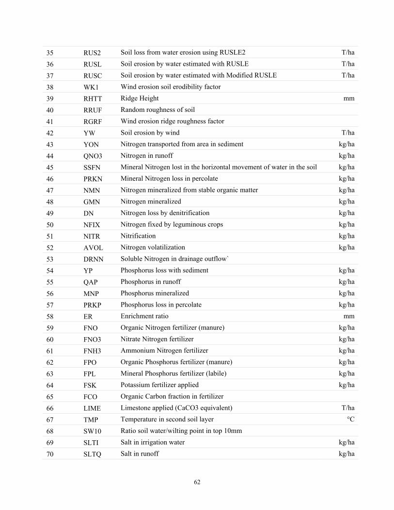
62

35 RUS2 Soil loss from water erosion using RUSLE2 T/ha

36 RUSL Soil erosion by water estimated with RUSLE T/ha

37 RUSC Soil erosion by water estimated with Modified RUSLE T/ha

38 WK1 Wind erosion soil erodibility factor

39 RHTT Ridge Height mm

40 RRUF Random roughness of soil

41 RGRF Wind erosion ridge roughness factor

42 YW Soil erosion by wind T/ha

43 YON Nitrogen transported from area in sediment kg/ha

44 QNO3 Nitrogen in runoff kg/ha

45 SSFN Mineral Nitrogen lost in the horizontal movement of water in the soil kg/ha

46 PRKN Mineral Nitrogen loss in percolate kg/ha

47 NMN Nitrogen mineralized from stable organic matter kg/ha

48 GMN Nitrogen mineralized kg/ha

49 DN Nitrogen loss by denitrification kg/ha

50 NFIX Nitrogen fixed by leguminous crops kg/ha

51 NITR Nitrification kg/ha

52 AVOL Nitrogen volatilization kg/ha

53 DRNN Soluble Nitrogen in drainage outflow`

54 YP Phosphorus loss with sediment kg/ha

55 QAP Phosphorus in runoff kg/ha

56 MNP Phosphorus mineralized kg/ha

57 PRKP Phosphorus loss in percolate kg/ha

58 ER Enrichment ratio mm

59 FNO Organic Nitrogen fertilizer (manure) kg/ha

60 FNO3 Nitrate Nitrogen fertilizer kg/ha

61 FNH3 Ammonium Nitrogen fertilizer kg/ha

62 FPO Organic Phosphorus fertilizer (manure) kg/ha

63 FPL Mineral Phosphorus fertilizer (labile) kg/ha

64 FSK Potassium fertilizer applied kg/ha

65 FCO Organic Carbon fraction in fertilizer

66 LIME Limestone applied (CaCO3 equivalent) T/ha

67 TMP Temperature in second soil layer °C

68 SW10 Ratio soil water/wilting point in top 10mm

69 SLTI Salt in irrigation water kg/ha

70 SLTQ Salt in runoff kg/ha

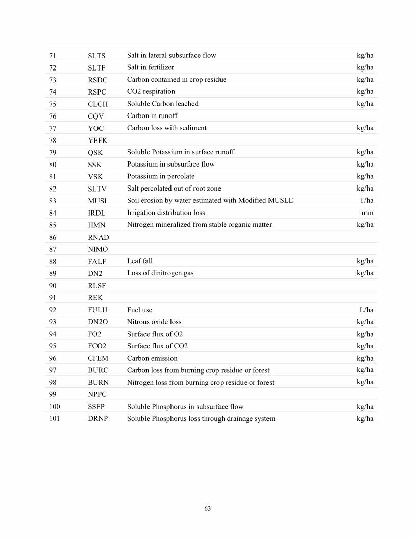
63

71 SLTS Salt in lateral subsurface flow kg/ha

72 SLTF Salt in fertilizer kg/ha

73 RSDC Carbon contained in crop residue kg/ha

74 RSPC CO2 respiration kg/ha

75 CLCH Soluble Carbon leached kg/ha

76 CQV Carbon in runoff

77 YOC Carbon loss with sediment kg/ha

78 YEFK

79 QSK Soluble Potassium in surface runoff kg/ha

80 SSK Potassium in subsurface flow kg/ha

81 VSK Potassium in percolate kg/ha

82 SLTV Salt percolated out of root zone kg/ha

83 MUSI Soil erosion by water estimated with Modified MUSLE T/ha

84 IRDL Irrigation distribution loss mm

85 HMN Nitrogen mineralized from stable organic matter kg/ha

86 RNAD

87 NIMO

88 FALF Leaf fall kg/ha

89 DN2 Loss of dinitrogen gas kg/ha

90 RLSF

91 REK

92 FULU Fuel use L/ha

93 DN2O Nitrous oxide loss kg/ha

94 FO2 Surface flux of O2 kg/ha

95 FCO2 Surface flux of CO2 kg/ha

96 CFEM Carbon emission kg/ha

97 BURC Carbon loss from burning crop residue or forest kg/ha

98 BURN Nitrogen loss from burning crop residue or forest kg/ha

99 NPPC

100 SSFP Soluble Phosphorus in subsurface flow kg/ha

101 DRNP Soluble Phosphorus loss through drainage system kg/ha

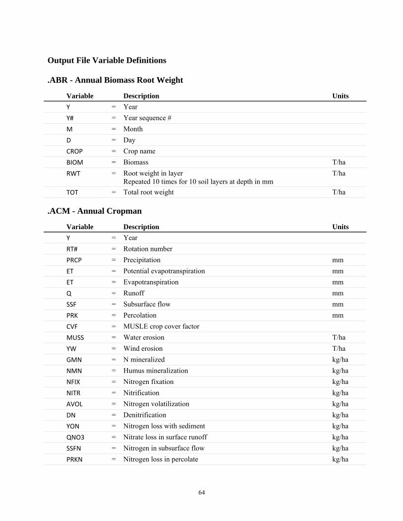
64

Output File Variable Definitions

.ABR - Annual Biomass Root Weight

Variable Description Units

Y = Year

Y# = Year sequence #

M = Month

D = Day

CROP = Crop name

BIOM = Biomass T/ha

RWT = Root weight in layer Repeated 10 times for 10 soil layers at depth in mm

T/ha

TOT = Total root weight T/ha

.ACM - Annual Cropman


Y = Year

RT# = Rotation number

PRCP = Precipitation mm

ET = Potential evapotranspiration mm

ET = Evapotranspiration mm

Q = Runoff mm

SSF = Subsurface flow mm

PRK = Percolation mm

CVF = MUSLE crop cover factor

MUSS = Water erosion T/ha

YW = Wind erosion T/ha

GMN = N mineralized kg/ha

NMN = Humus mineralization kg/ha

NFIX = Nitrogen fixation kg/ha

NITR = Nitrification kg/ha

AVOL = Nitrogen volatilization kg/ha

DN = Denitrification kg/ha

YON = Nitrogen loss with sediment kg/ha

QNO3 = Nitrate loss in surface runoff kg/ha

SSFN = Nitrogen in subsurface flow kg/ha

PRKN = Nitrogen loss in percolate kg/ha

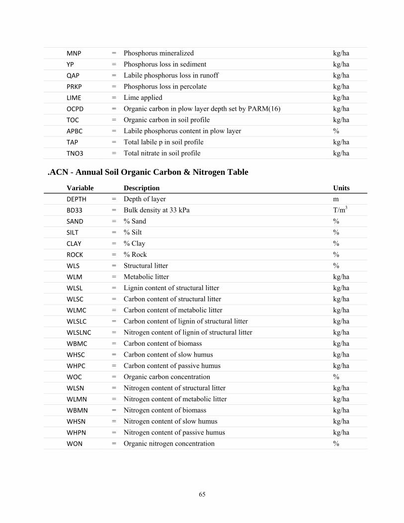
65

MNP = Phosphorus mineralized kg/ha

YP = Phosphorus loss in sediment kg/ha

QAP = Labile phosphorus loss in runoff kg/ha

PRKP = Phosphorus loss in percolate kg/ha

LIME = Lime applied kg/ha

OCPD = Organic carbon in plow layer depth set by PARM(16) kg/ha

TOC = Organic carbon in soil profile kg/ha

APBC = Labile phosphorus content in plow layer %

TAP = Total labile p in soil profile kg/ha

TNO3 = Total nitrate in soil profile kg/ha

.ACN - Annual Soil Organic Carbon & Nitrogen Table


DEPTH = Depth of layer m

BD33 = Bulk density at 33 kPa T/m3

SAND = % Sand %

SILT = % Silt %

CLAY = % Clay %

ROCK = % Rock %

WLS = Structural litter %

WLM = Metabolic litter kg/ha

WLSL = Lignin content of structural litter kg/ha

WLSC = Carbon content of structural litter kg/ha

WLMC = Carbon content of metabolic litter kg/ha

WLSLC = Carbon content of lignin of structural litter kg/ha

WLSLNC = Nitrogen content of lignin of structural litter kg/ha

WBMC = Carbon content of biomass kg/ha

WHSC = Carbon content of slow humus kg/ha

WHPC = Carbon content of passive humus kg/ha

WOC = Organic carbon concentration %

WLSN = Nitrogen content of structural litter kg/ha

WLMN = Nitrogen content of metabolic litter kg/ha

WBMN = Nitrogen content of biomass kg/ha

WHSN = Nitrogen content of slow humus kg/ha

WHPN = Nitrogen content of passive humus kg/ha

WON = Organic nitrogen concentration %

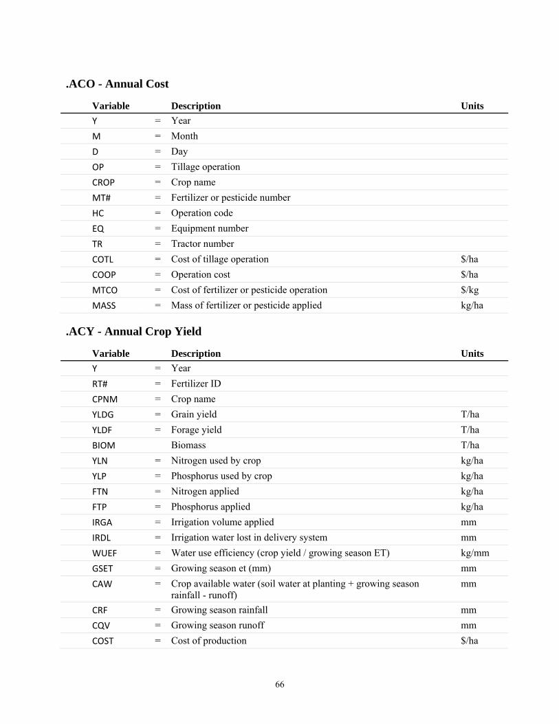
66

.ACO - Annual Cost


Y = Year

M = Month

D = Day

OP = Tillage operation

CROP = Crop name

MT# = Fertilizer or pesticide number

HC = Operation code

EQ = Equipment number

TR = Tractor number

COTL = Cost of tillage operation $/ha

COOP = Operation cost $/ha

MTCO = Cost of fertilizer or pesticide operation $/kg

MASS = Mass of fertilizer or pesticide applied kg/ha

.ACY - Annual Crop Yield


Y = Year

RT# = Fertilizer ID

CPNM = Crop name

YLDG = Grain yield T/ha

YLDF = Forage yield T/ha

BIOM Biomass T/ha

YLN = Nitrogen used by crop kg/ha

YLP = Phosphorus used by crop kg/ha

FTN = Nitrogen applied kg/ha

FTP = Phosphorus applied kg/ha

IRGA = Irrigation volume applied mm

IRDL = Irrigation water lost in delivery system mm

WUEF = Water use efficiency (crop yield / growing season ET) kg/mm

GSET = Growing season et (mm) mm

CAW = Crop available water (soil water at planting + growing season rainfall - runoff)

mm

CRF = Growing season rainfall mm

CQV = Growing season runoff mm

COST = Cost of production $/ha

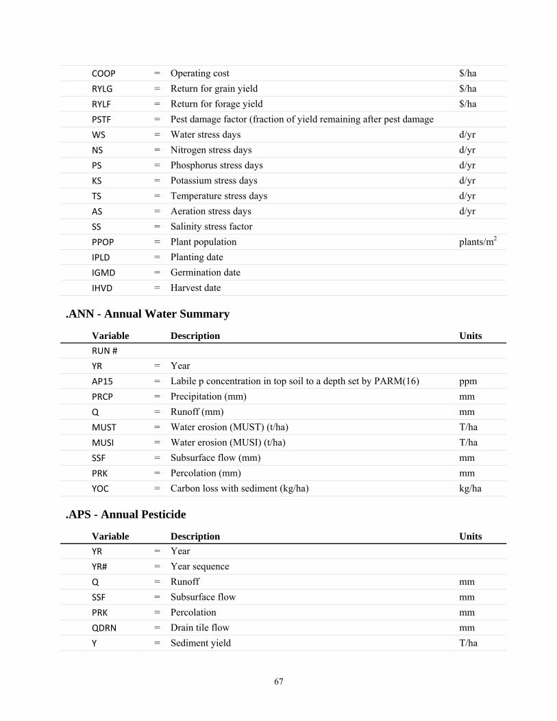
67

COOP = Operating cost $/ha

RYLG = Return for grain yield $/ha

RYLF = Return for forage yield $/ha

PSTF = Pest damage factor (fraction of yield remaining after pest damage

WS = Water stress days d/yr

NS = Nitrogen stress days d/yr

PS = Phosphorus stress days d/yr

KS = Potassium stress days d/yr

TS = Temperature stress days d/yr

AS = Aeration stress days d/yr

SS = Salinity stress factor

PPOP = Plant population plants/m2

IPLD = Planting date

IGMD = Germination date

IHVD = Harvest date

.ANN - Annual Water Summary


RUN #

YR = Year

AP15 = Labile p concentration in top soil to a depth set by PARM(16) ppm

PRCP = Precipitation (mm) mm

Q = Runoff (mm) mm

MUST = Water erosion (MUST) (t/ha) T/ha

MUSI = Water erosion (MUSI) (t/ha) T/ha

SSF = Subsurface flow (mm) mm

PRK = Percolation (mm) mm

YOC = Carbon loss with sediment (kg/ha) kg/ha

.APS - Annual Pesticide


YR = Year

YR# = Year sequence

Q = Runoff mm



QDRN = Drain tile flow mm

Y = Sediment yield T/ha

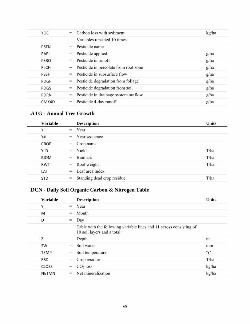
68

YOC = Carbon loss with sediment kg/ha

Variables repeated 10 times

PSTN = Pesticide name

PAPL = Pesticide applied g/ha

PSRO = Pesticide in runoff g/ha

PLCH = Pesticide in percolate from root zone g/ha

PSSF = Pesticide in subsurface flow g/ha

PDGF = Pesticide degradation from foliage g/ha

PDGS = Pesticide degradation from soil g/ha

PDRN = Pesticide in drainage system outflow g/ha

CMX4D = Pesticide 4-day runoff g/ha

.ATG - Annual Tree Growth


Y = Year

Y# = Year sequence

CROP = Crop name

YLD = Yield T/ha

BIOM = Biomass T/ha

RWT = Root weight T/ha

LAI = Leaf area index

STD = Standing dead crop residue T/ha

.DCN - Daily Soil Organic Carbon & Nitrogen Table


Y = Year

M = Month

D = Day

Table with the following variable lines and 11 across consisting of 10 soil layers and a total:

Z Depth m

SW = Soil water mm

TEMP = Soil temperature °C

RSD = Crop residue T/ha

CLOSS = CO2 loss kg/ha

NETMN = Net mineralization kg/ha

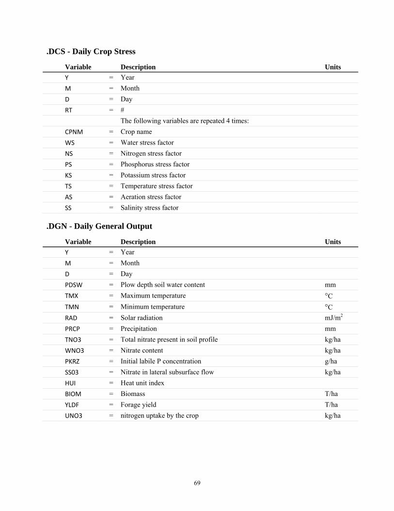
69

.DCS - Daily Crop Stress


Y = Year

M = Month

D = Day

RT = #

The following variables are repeated 4 times:

CPNM = Crop name

WS = Water stress factor

NS = Nitrogen stress factor

PS = Phosphorus stress factor

KS = Potassium stress factor

TS = Temperature stress factor

AS = Aeration stress factor


.DGN - Daily General Output


Y = Year

M = Month

D = Day

PDSW = Plow depth soil water content mm

TMX = Maximum temperature °C

TMN = Minimum temperature °C

RAD = Solar radiation mJ/m2


TNO3 = Total nitrate present in soil profile kg/ha

WNO3 = Nitrate content kg/ha

PKRZ = Initial labile P concentration g/ha

SS03 = Nitrate in lateral subsurface flow kg/ha

HUI = Heat unit index

BIOM = Biomass T/ha

YLDF = Forage yield T/ha

UNO3 = nitrogen uptake by the crop kg/ha

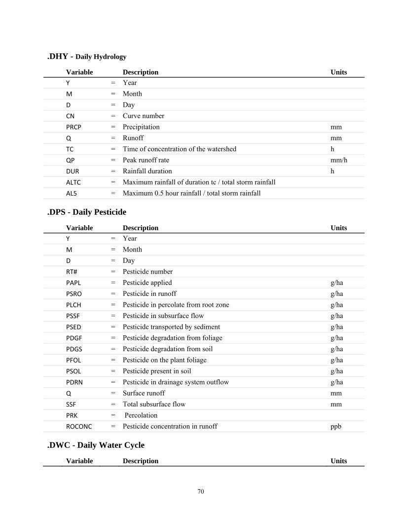
70

.DHY - Daily Hydrology


Y = Year

M = Month

D = Day

CN = Curve number


Q = Runoff mm

TC = Time of concentration of the watershed h

QP = Peak runoff rate mm/h

DUR = Rainfall duration h

ALTC = Maximum rainfall of duration tc / total storm rainfall

AL5 = Maximum 0.5 hour rainfall / total storm rainfall

.DPS - Daily Pesticide


Y = Year

M = Month

D = Day

RT# = Pesticide number

PAPL = Pesticide applied g/ha

PSRO = Pesticide in runoff g/ha

PLCH = Pesticide in percolate from root zone g/ha

PSSF = Pesticide in subsurface flow g/ha

PSED = Pesticide transported by sediment g/ha

PDGF = Pesticide degradation from foliage g/ha

PDGS = Pesticide degradation from soil g/ha

PFOL = Pesticide on the plant foliage g/ha

PSOL = Pesticide present in soil g/ha

PDRN = Pesticide in drainage system outflow g/ha

Q = Surface runoff mm

SSF = Total subsurface flow mm

PRK = Percolation

ROCONC = Pesticide concentration in runoff ppb

.DWC - Daily Water Cycle


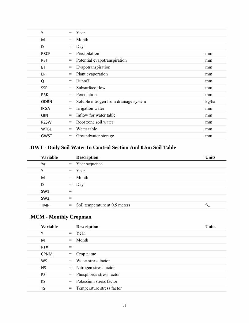
71

Y = Year

M = Month

D = Day


PET = Potential evapotranspiration mm


EP = Plant evaporation mm

Q = Runoff mm



QDRN = Soluble nitrogen from drainage system kg/ha

IRGA = Irrigation water mm

QIN = Inflow for water table mm

RZSW = Root zone soil water mm

WTBL = Water table mm

GWST = Groundwater storage mm

.DWT - Daily Soil Water In Control Section And 0.5m Soil Table


Y# = Year sequence

Y = Year

M = Month

D = Day

SW1 =

SW2 =

TMP = Soil temperature at 0.5 meters °C

.MCM - Monthly Cropman


Y = Year

M = Month

RT# =

CPNM = Crop name

WS = Water stress factor

NS = Nitrogen stress factor

PS = Phosphorus stress factor

KS = Potassium stress factor

TS = Temperature stress factor

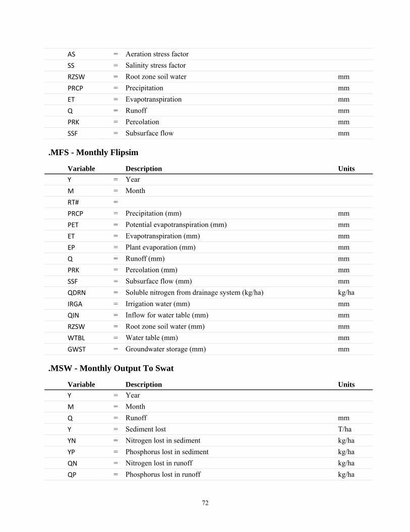
72

AS = Aeration stress factor





Q = Runoff mm



.MFS - Monthly Flipsim


Y = Year

M = Month

RT# =

PRCP = Precipitation (mm) mm

PET = Potential evapotranspiration (mm) mm

ET = Evapotranspiration (mm) mm

EP = Plant evaporation (mm) mm

Q = Runoff (mm) mm

PRK = Percolation (mm) mm

SSF = Subsurface flow (mm) mm

QDRN = Soluble nitrogen from drainage system (kg/ha) kg/ha

IRGA = Irrigation water (mm) mm

QIN = Inflow for water table (mm) mm

RZSW = Root zone soil water (mm) mm

WTBL = Water table (mm) mm

GWST = Groundwater storage (mm) mm

.MSW - Monthly Output To Swat


Y = Year

M = Month

Q = Runoff mm

Y = Sediment lost T/ha

YN = Nitrogen lost in sediment kg/ha

YP = Phosphorus lost in sediment kg/ha

QN = Nitrogen lost in runoff kg/ha

QP = Phosphorus lost in runoff kg/ha

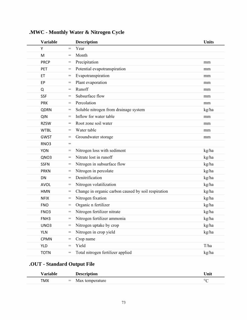
73

.MWC - Monthly Water & Nitrogen Cycle


Y = Year

M = Month


PET = Potential evapotranspiration mm



Q = Runoff mm



QDRN = Soluble nitrogen from drainage system kg/ha

QIN = Inflow for water table mm


WTBL = Water table mm

GWST = Groundwater storage mm

RNO3 =

YON = Nitrogen loss with sediment kg/ha

QNO3 = Nitrate lost in runoff kg/ha

SSFN = Nitrogen in subsurface flow kg/ha

PRKN = Nitrogen in percolate kg/ha


AVOL = Nitrogen volatilization kg/ha

HMN = Change in organic carbon caused by soil respiration kg/ha


FNO = Organic n fertilizer kg/ha

FNO3 = Nitrogen fertilizer nitrate kg/ha

FNH3 = Nitrogen fertilizer ammonia kg/ha

UNO3 = Nitrogen uptake by crop kg/ha

YLN = Nitrogen in crop yield kg/ha

CPMN = Crop name

YLD = Yield T/ha

TOTN = Total nitrogen fertilizer applied kg/ha

.OUT - Standard Output File

Variable Description Unit

TMX = Max temperature °C

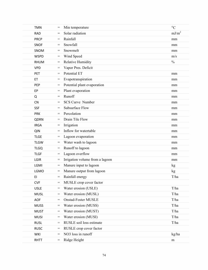
74

TMN = Min temperature °C

RAD = Solar radiation mJ/m2

PRCP = Rainfall mm

SNOF = Snowfall mm

SNOM = Snowmelt mm

WSPD = Wind Speed m/s

RHUM = Relative Humidity %

VPD = Vapor Pres. Deficit

PET = Potential ET mm


PEP = Potential plant evaporation mm


Q = Runoff mm

CN = SCS Curve Number mm

SSF = Subsurface Flow mm


QDRN = Drain Tile Flow mm

IRGA = Irrigation mm

QIN = Inflow for watertable mm

TLGE = Lagoon evaporation mm

TLGW = Water wash to lagoon mm

TLGQ = Runoff to lagoon mm

TLGF = Lagoon overflow mm

LGIR = Irrigation volume from a lagoon mm

LGMI = Manure input to lagoon kg

LGMO = Manure output from lagoon kg

EI = Rainfall energy T/ha

CVF = MUSLE crop cover factor

USLE = Water erosion (USLE) T/ha

MUSL = Water erosion (MUSL) T/ha

AOF = Onstad-Foster MUSLE T/ha

MUSS = Water erosion (MUSS) T/ha

MUST = Water erosion (MUST) T/ha

MUSI = Water erosion (MUSI) T/ha

RUSL = RUSLE soil loss estimate T/ha

RUSC = RUSLE crop cover factor

WKI = NO3 loss in runoff kg/ha

RHTT = Ridge Height m

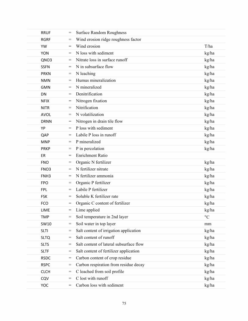
75

RRUF = Surface Random Roughness

RGRF = Wind erosion ridge roughness factor

YW = Wind erosion T/ha

YON = N loss with sediment kg/ha

QNO3 = Nitrate loss in surface runoff kg/ha

SSFN = N in subsurface flow kg/ha

PRKN = N leaching kg/ha

NMN = Humus mineralization kg/ha

GMN = N mineralized kg/ha



NITR = Nitrification kg/ha

AVOL = N volatilization kg/ha

DRNN = Nitrogen in drain tile flow kg/ha

YP = P loss with sediment kg/ha

QAP = Labile P loss in runoff kg/ha

MNP = P mineralized kg/ha

PRKP = P in percolation kg/ha

ER = Enrichment Ratio

FNO = Organic N fertilizer kg/ha

FNO3 = N fertilizer nitrate kg/ha

FNH3 = N fertilizer ammonia kg/ha

FPO = Organic P fertilizer kg/ha

FPL = Labile P fertilizer kg/ha

FSK = Soluble K fertilizer rate kg/ha

FCO = Organic C content of fertilizer kg/ha

LIME = Lime applied kg/ha

TMP = Soil temperature in 2nd layer °C

SW10 = Soil water in top layer mm

SLTI = Salt content of irrigation application kg/ha

SLTQ = Salt content of runoff kg/ha

SLTS = Salt content of lateral subsurface flow kg/ha

SLTF = Salt content of fertilizer application kg/ha

RSDC = Carbon content of crop residue kg/ha

RSPC = Carbon respiration from residue decay kg/ha

CLCH = C leached from soil profile kg/ha

CQV = C lost with runoff kg/ha

YOC = Carbon loss with sediment kg/ha

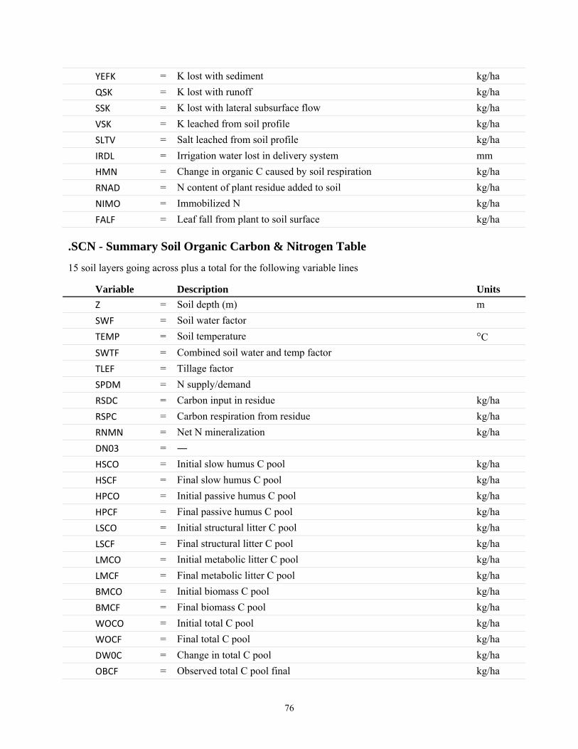
76

YEFK = K lost with sediment kg/ha

QSK = K lost with runoff kg/ha

SSK = K lost with lateral subsurface flow kg/ha

VSK = K leached from soil profile kg/ha

SLTV = Salt leached from soil profile kg/ha

IRDL = Irrigation water lost in delivery system mm

HMN = Change in organic C caused by soil respiration kg/ha

RNAD = N content of plant residue added to soil kg/ha

NIMO = Immobilized N kg/ha

FALF = Leaf fall from plant to soil surface kg/ha

.SCN - Summary Soil Organic Carbon & Nitrogen Table

15 soil layers going across plus a total for the following variable lines


Z = Soil depth (m) m

SWF = Soil water factor

TEMP = Soil temperature °C

SWTF = Combined soil water and temp factor

TLEF = Tillage factor

SPDM = N supply/demand

RSDC = Carbon input in residue kg/ha

RSPC = Carbon respiration from residue kg/ha

RNMN = Net N mineralization kg/ha

DN03 = ―

HSCO = Initial slow humus C pool kg/ha

HSCF = Final slow humus C pool kg/ha

HPCO = Initial passive humus C pool kg/ha

HPCF = Final passive humus C pool kg/ha

LSCO = Initial structural litter C pool kg/ha

LSCF = Final structural litter C pool kg/ha

LMCO = Initial metabolic litter C pool kg/ha

LMCF = Final metabolic litter C pool kg/ha

BMCO = Initial biomass C pool kg/ha

BMCF = Final biomass C pool kg/ha

WOCO = Initial total C pool kg/ha

WOCF = Final total C pool kg/ha

DW0C = Change in total C pool kg/ha

OBCF = Observed total C pool final kg/ha

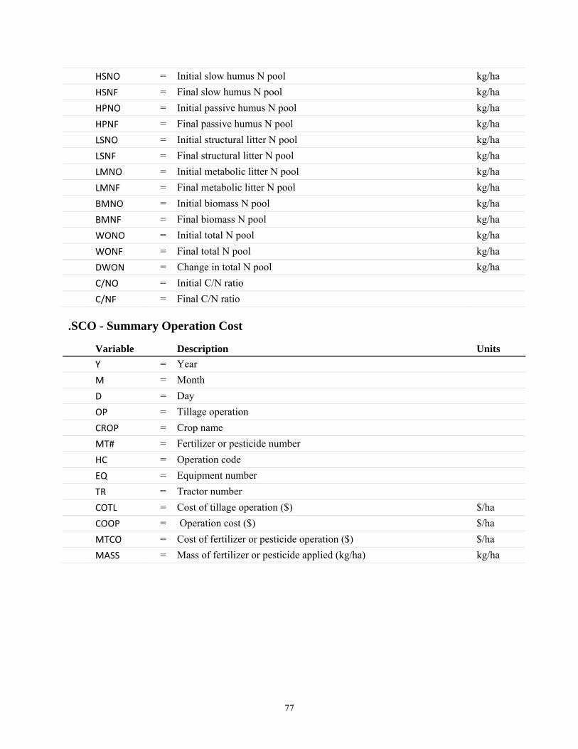
77

HSNO = Initial slow humus N pool kg/ha

HSNF = Final slow humus N pool kg/ha

HPNO = Initial passive humus N pool kg/ha

HPNF = Final passive humus N pool kg/ha

LSNO = Initial structural litter N pool kg/ha

LSNF = Final structural litter N pool kg/ha

LMNO = Initial metabolic litter N pool kg/ha

LMNF = Final metabolic litter N pool kg/ha

BMNO = Initial biomass N pool kg/ha

BMNF = Final biomass N pool kg/ha

WONO = Initial total N pool kg/ha

WONF = Final total N pool kg/ha

DWON = Change in total N pool kg/ha

C/NO = Initial C/N ratio

C/NF = Final C/N ratio

.SCO - Summary Operation Cost


Y = Year

M = Month

D = Day

OP = Tillage operation

CROP = Crop name

MT# = Fertilizer or pesticide number

HC = Operation code

EQ = Equipment number

TR = Tractor number

COTL = Cost of tillage operation ($) $/ha

COOP = Operation cost ($) $/ha

MTCO = Cost of fertilizer or pesticide operation ($) $/ha

MASS = Mass of fertilizer or pesticide applied (kg/ha) kg/ha

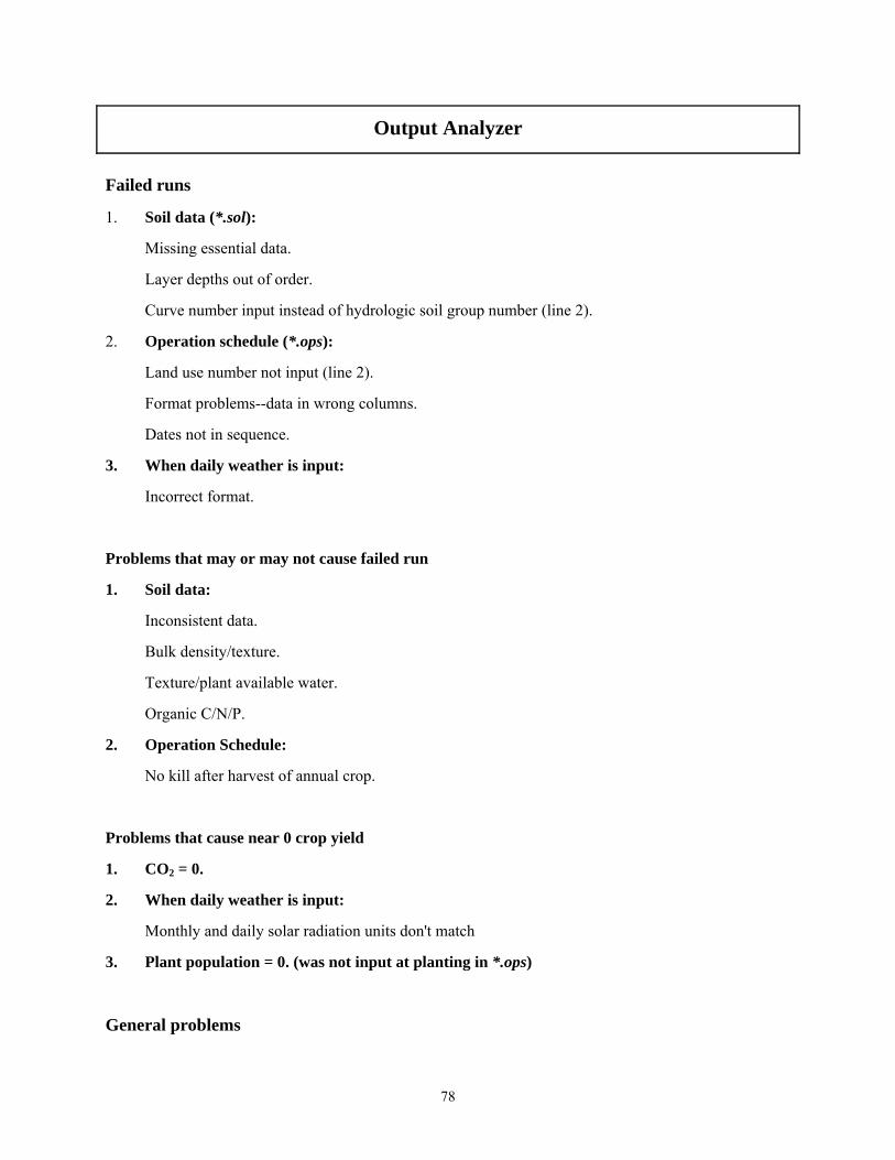
78

Output Analyzer

Failed runs

1. Soil data (*.sol):

Missing essential data.

Layer depths out of order.

Curve number input instead of hydrologic soil group number (line 2).

2. Operation schedule (*.ops):

Land use number not input (line 2).

Format problems--data in wrong columns.

Dates not in sequence.

3. When daily weather is input:

Incorrect format.

Problems that may or may not cause failed run

1. Soil data:

Inconsistent data.

Bulk density/texture.

Texture/plant available water.

Organic C/N/P.

2. Operation Schedule:

No kill after harvest of annual crop.

Problems that cause near 0 crop yield

1. CO2 = 0.


Monthly and daily solar radiation units don't match

3. Plant population = 0. (was not input at planting in *.ops)

General problems

79

1. Working files don't match those contained in EPICFILE.dat

For example you are working with CROP0810. dat and EPICFILE. dat contains USERCROP. dat.


The date must be input on the first line (year, month, day)--format is (2X, 3I4). The beginning simulation date in EPICCONT.dat must be equal or greater than the one appearing on line one of the weather file (*.wth).

Completed runs--examine *.out files

Select monthly output in EPICCONT.dat (IPD = 3).

Preliminary investigation

Check nutrient and water balances for each run (look for BALANCE). They should be near 0.

Check water balance for the entire watershed (TOTAL WATER BALANCE).

Check average annual surface runoff, water yield, and sediment and nutrient

Runoff problems--things to check

1. PET is not reasonable:

Try another PET eq that may be more appropriate for the site. Hargreaves is the most robust and can be adjusted by varying the coefficient (PARM(23)0.0023-0.0032) or the exponential (PARM(34) 0.5-0.6) in PARM0810.DAT. Penman-Monteith is generally considered the most accurate but is sensitive to wind speed which is subject to measurement errors. It can also be adjusted through the stomatal conductance coefficient (PARM(1)1.0-2.0) in PARM0810.DAT. The Baier-Robertson equation developed in Canada is a good choice in cold climates.

2. ET is not reasonable:

Crop growing season may be incorrect--check planting and harvest dates and potential heat units

(crg.ops). Also check harvest time each year in txbell.out for the value of HUSC (look for CORN

YLD=). HUSC should normally range from 1. to 1.2. If HUSC is < 1. PHU is too large or harvest

date is too early. If HUSC is > 1.2 PHU is too small or harvest date is too late. For many annual crops the value of HUSC should be set to 1.2 using an early harvest date (crg.ops). Harvest can't occur until the input harvest date and then only after the accumulated heat units have reached the input HUSC value. Forage crops may be grazed too closely or cut too often to allow leaf area to develop properly for normal plant water use.

3. Check Runoff equations:

NRCS curve number equation: The CN equation varies with soil water. EPIC has four different methods of linking CN and soil

80

water plus a constant CN option. The methods are:

1. Variable daily CN nonlinear CN/SW with depth soil water weighting.

2. Variable daily CN nonlinear CN/SW no depth weighting.

3. Variable daily CN linear CN/SW no depth weighting

4. Non-Varying CN--CN2 used for all storms.

5. Variable Daily CN SMI (Soil Moisture Index)

Generally the soil moisture index (5)is the most robust and reliable because it is not sensitive to errors in soil data. This method is adjustable using PARM(42) (PARM0810.DAT). PARM(42) usually is in the range 0.5-2.0 (small values reduce runoff). The nonlinear forms (1,2) also perform very well in many situations. The constant CN method (4) is a good choice when soil water is not a dominant factor.

Green and Ampt infiltration equation:

The G&A equation is available for use in special cases where CN is not performing well. The three variations of G&A are:

1. Rainfall intensity is simulated with a double exponential distribution and peak rainfall rate is simulated independently.

2. Same as (1) except peak rainfall rate is input.

3. Rainfall intensity is uniformly distributed and peak rainfall rate is input (useful in rainfall simulator studies).

4. Erosion/sedimentation problems:

1. Runoff must be realistic.

2. Crop growth must be realistic to provide proper cover and residue.

3. Tillage must mix residue with soil properly.

4. Erosion equations:

The USLE and five modifications are available. MUSLE, MUSS, and MUST usually give similar results and are appropriate for estimating sediment yield from small watersheds up to about 250 km2. The USLE is an erosion equation that is useful in studies like assessing the effect of erosion on productivity.

5. Slope length and steepness factor:

Both USLE and RUSLE equations are available. RUSLE is preferred for steep slopes > 20%.

6. Crop growth:

In *.out go to AVE ANNUAL CROP YLD and AVE STRESS DAYS. The stress days reveal the stresses that are

constraining crop growth.

Root growth stresses of bulk density (BD) or aluminum saturation (ALSAT) can reduce crop yields

81

greatly. Go to SOIL PHYSICAL DATA and check for unreasonably high BD. Go to SOIL CHEMICAL DATA

and check for high aluminum saturation values > 90 caused by low pH <5. BD can be lowered by deep tillage or simply corrected if the data are erroneous. Aluminum saturation can be lowered by applying lime or by correcting erroneous pH data.

Water stress is the most common constraint to crop growth. Excessive PET or runoff estimates are major causes. Plant available water is another important limitation that causes water stress. Erroneous estimates of plant available water occur when field capacity or wilting point are incorrect. Soil water storage is particularly important in dry climates.

Nitrogen and Phosphorus stress is caused by low mineralization rates, inadequate fertilizer, or excessive

leaching of N. Go to SOIL CHEMICAL DATA and examine organic N, P, and C. C/N should be near 10. N/P

should be near 8. The mineralization rate can be increased by decreasing the number of years of

cultivation at the beginning of simulation (*.sol line 3). Check N leaching in the last table (AVERAGE

ANNUAL DATA) under QNO3. If large values relative to annual N fertilizer are found go to SUMMARY

TABLE and look at PRKN and PRK. High percolation values (PRK) may result from low ET or runoff,

low soil plant available water storage (FC -WP), or high saturated conductivity values. PRK is sensitive to the user choice to use manual irrigation applications of rigid amounts.

82

How to Validate Crop Yields

USER NOTE OF CAUTION: If a multiple-run has been executed (denoted by a value greater than zero in col. 4 in MLRN0810.DAT) and the pre-run results are of no interest, then open *.out and go to or find

TOTAL WATER BALANCE. The applicable simulation results follow this section beginning with a new epic

descriptive title. Likewise, use only the second set of results given in *.man. *.asa, *.asw, *.wss, *.msw, etc. files.

First, check the accuracy of soil depths if specific simulated yields are low-

To determine if soil depth and the important related water-holding capacity is curtailing a specific crop yield, open the *.acy file where both grain and forage yields are listed by crop. Data entry errors in the depth of soil data can be checked by opening the appropriate *.sol file and referring to the accumulated depth (m) of the last soil layer.

Second, check the accuracy of the heat units from planting to harvest

-After completing a run if automatic heat unit scheduling is not selected in EPICCONT.dat (line 1:

IHUS), open the *.out file and find TOTAL WATER BALANCE, scroll down a few lines to the beginning

of the appropriate simulation to SA(# ID). Scroll down until a HARV operation is found. This is a list of

harvest operations in year 1 for each subarea. Scroll to the right to HUSC= for each crop harvested. If

any HUSC values for a crop are outside the range of 0.9 to 1.1, scroll down to check following years. If all years are outside the range, check both the planting (above the harvest operations) and the harvest date for accuracy. If they are accurate to the best of your knowledge, then open the appropriate *.ops file(s) which contains the specific crop for which the heat units need adjusted. If HUSC in the *.out file is less than 1.0, decrease the heat units at the planting operation and if greater than 1.0, increase the heat units.

If automatic heat unit scheduling is selected in EPICCONT.dat (line 1: IHUS), open the *.out file and

follow the same procedure as above except instead of changing the heat units, change either the plant or harvest date to result in a more optimum HUSC = approx. 1.0 in the *.out file for the HARV operation.

Third, check the plant population for accuracy- If a crop yield is too low, check the plant population in the *.ops file. Correct to the best of your knowledge. Increasing (Decreasing) it will increase (lower) the simulated yield. Increasing plant population usually increases yield but not always—sometimes in very dry climates lower populations

produce more yield.

Fourth, check plant stress levels if a crop yield is low- To determine the cause of stress to biomass and root development from lack of water, nutrients, bulk density, excessive aluminum toxicity, or insufficient air for biomass or roots, open the *.out file and

find TOTAL WATER BALANCE and then find AVE ANNUAL CROP YLD DATA. If the crop of interest is

not in the first listing, scroll down to subsequent listings. Then scroll to the right of the screen and view the stress days for the crop. If a large number of days of N stress are observed, for example, open the *.ops file(s) that contains the stressed crop(s) and add more N fertilizer; continue to do the

83

same for the crop(s) with P stress, and if irrigation is being applied manually and water stress days are high, add more irrigations if appropriate. In contrast, if air stress days are high in either roots or biomass, reduce irrigation applications. Aluminum toxicity stress is usually a soil condition treated by adding lime (automatically applied if selected in the *.sub file, line 7). If soil bulk density causes root stress, check all *.sol file(s) for errors in the bulk density data entries for each subarea that produces the affected crop. Also, check PARM(2)—the original value is 1.15 but may need increasing to 1.5

for many cases to reduce bulk density stress. Setting PARM(2) to 2.0 eliminates all root stresses.

Fifth, check the leaf area index (MXLA)- To determine if the leaf area setting is inadequate for optimum yields of a crop, open *.out and find

CROP PARAMETERS. Scroll down to a row indicating MXLA for the value of a low yielding crop and

compare it with the value DMLA in line 1 of the CROP0810.dat file for the appropriate crop. In the

Crop Parameters table each row with the same parameter name a different subarea. If the two leaf area indices are near equal and the crop yield is low, increase the index value in CROP0810.dat.

DMLA is set at the maximum LAI that the crop can obtain under ideal conditions so it seldom needs

increasing. MXLA the adjusted DMLA based on plant population can be increased by increasing

population.

Sixth, revise the Harvest Index and Biomass-Energy Ratios- If after the first five checks are completed and crop yields remain inaccurate, some basic crop parameters can be revised as a last resort. Normally these parameters are not to be revised, being accurate for crops in the U.S. They may need to be revised slightly for international use. In CROP0810.dat, the harvest index (HI) relates to the grain yield only as a ratio of the above-ground biomass. The higher the ratio, the more grain yield reported for a given level of biomass. Similarly, the biomass to energy ratio (WA) increases yields through biomass changes and, therefore, both grain

and forage yields increase.

84

How to Validate Runoff, Sediment Losses & Sediment Losses

USER NOTE OF CAUTION: If a multiple-run has been executed (denoted by a value greater than zero

in col. 4 in MLRN0810.dat) and the pre-run results are of no interest, then open *.out and find TOTAL

WATER BALANCE. The applicable simulation results follow this section beginning with a new EPIC

descriptive title.

Likewise, use only the second set of results given in *.man. *.asa, *.asw, *.wss, *.msw, etc. files.

TO CHECK THE ACCURACY OF SIMULATED RUNOFF/SEDIMENT LOSSES AND SEDIMENT LOSSES FOR THE WATERSHED OUTLET, open the *.asw file for the yearly simulated losses and

consult your EPIC0810 manual for the definitions of the column headings. If QTW values for the years

being validated are unacceptable, usually YW will also be in error, follow the instructions below:

First, check land use values- Correct runoff/sediment losses by checking the accuracy of estimated curve numbers that dictate

runoff/sediment losses. This may be done by checking the land use number in line 2 (LUN) of each

*.ops file. If multiple crop rotations are used, simulated runoff/sediment losses accuracy will be

enhanced if LUN is revised at planting and harvest of each crop by entering a value on the appropriate

operation line.

Second, check hydrologic soil group values-

Correct runoff/sediment losses by checking the accuracy of the hydrologic soil group in line 2 (HSG)

in each of the *.sol files.

Third, check upland and chanel hydrology values- Correct runoff/sediment losses by checking the hydrology of the subareas. Open the *.out file and

find HYDROLOGIC DATA which describes the channel and upland hydrology of each subarea. Note:

check the accuracy of each subarea upland and channel slopes.

Fourth, check monthly and annual rainfall values- Correct runoff/sediment losses by checking the simulated monthly and annual rainfall for the years being validated in the *.wss file.

Fifth, check the saturated conductivity values for soils- Correct runoff/sediment losses by checking the accuracy of the saturated conductivity values of each

soil.

Sixth, check the accuracy of the erosion control practice factor- Correct runoff/sediment losses by checking the accuracy of the erosion control practice factor in line

9 (PEC) of each *.ops file.

Seventh, check the choice of water erosion equation-

85

For watershed analyses, sediment losses need to be indicated with the recommended choices of #3

(MUSS) or #0 (MUST).

Eighth, revise the method of calculating the daily adjusted curve numbers- Revise the method of calculating daily adjusted curve numbers in line 2 of each *.sub file. Usually #4

or #0 are recommended.

Nineth, revise the irrigation runoff ratios if irrigation operations are used- Revise the global irrigation runoff ratio in line 8 of each *.sub file or for individual irrigation applications, the runoff ratio may be entered on the line of the irrigation operation in each *.ops file having irrigated crops.

NOTE: if automatic irrigation has been selected with a value = 0.0 in line 7 (NIRR) of each *.sub file

that is irrigated, irrigation runoff will be significantly lower than when using rigid applications of the

amounts indicated in the *.ops files.

What type of runoff is in error, Q, SSF, QRF, QDRN, or RTF?

If Q and/or QDRN are in error, follow the next twelve steps. If SSF, QRF, and RTF are in error, go to

the next � item.

First, check land use (curve number) values Correct runoff/sediment losses by checking the accuracy of estimated curve numbers that dictate runoff/sediment losses. This may be done by checking the land use number in line 2 (LUN) of each *.ops file. If multiple crop rotations are used, simulated runoff/sediment losses accuracy will be enhanced if LUN is revised at planting and harvest of each crop by entering a value on the

appropriate operation line. NOTE: Land use numbers may be substituted with curve numbers.

Second, check the saturated conductivity values for soils Correct runoff/sediment losses by checking the accuracy of the saturated conductivity values of each

soil in the *.sol files.

Third, check hydrologic soil group values Correct runoff/sediment losses by checking the accuracy of the hydrologic soil group in line 2 (HSG) in each of the *.sol files. This value should be consistent with the % sand, % silt, and the residual %

clay.

Fourth, check upland and channel hydrology values Correct runoff/sediment losses by checking the hydrology of the subareas. Open the *.out file and

find HYDROLOGIC DATA which describes the channel and upland hydrology of each subarea. Note:

check the accuracy of each subarea upland and channel slopes.

Fifth, check monthly and annual rainfall values Correct runoff/sediment losses by checking the simulated annual rainfall for the years being validated

86

in the *.aws file. To determine the monthly average rainfall for the years simulated, open the *.wss

file and again go to the second set of results to find the row with ―PRCPǁ.

Sixth, check the accuracy of the erosion control practice factor Correct runoff/sediment losses by checking the accuracy of the erosion control practice factor in line

9 (PEC) of each *.sub file.

Seventh, check the choice of water erosion equation For watershed analyses, open EPICCONT.dat, line 5 (DRV), where sediment losses need to be

indicated with the recommended choices of #3 (MUSS) or #0 (MUST).

Eighth, revise the method of calculating the daily adjusted curve numbers- Revise the method of calculating daily adjusted curve numbers in line 2 of each *.sub file. Usually #4 or #0 are recommended. The choice made for a run can be checked by opening *.out and finding

VARIABLE CN.

Nineth, revise the irrigation runoff ratios if irrigation operations are used Revise the global irrigation runoff ratio in line 8 of each *.sub file or for individual irrigation applications, the runoff ratio may be entered on the line of the irrigation operation in each *.ops file having irrigated crops.

NOTE: if automatic irrigation has been selected with a value = 0.0 in line 7 (NIRR) of each *.sub file that is irrigated, irrigation runoff will be significantly lower than when using rigid applications of the

amounts indicated in the *.ops files.

Tenth, revise the land uses To check the accuracy of the land use by major land use category such as forest, grass, and crops,

open the *.out file and find LAND USE SUMMARY. This listing provides the proportionate breakdown

of the watershed into the land uses by crop or other use.

NOTE: Since runoff and erosion are highly correlated with cropland and its land condition (straight row, contoured, contoured and terraced), carefully verify the proportion of each crop in the watershed

in this listing.

To check another runoff component: RTF

Open EPICCONT.dat and determine the value of RFPO on line 4, fourth variable. If this is 0.0,

change it to 0.01 or higher until you have validated RTF.

To check other runoff components: SSF and QRF-

Open each *.sol file and determine the value for each layer of HCL, line 23. If this is 0.0, change it to

0.1 or higher until SSF and/or QRF are validated.

After validating runoff, check MUST or MUSS for accuracy.

87

To validate erosion, adjust PARM(46) for a more accurate simulation of MUST/MUSS. Increasing

PARM(46) increases the effect of crop residue and therefore reduces erosion.

88

Pesticide Fate – The GLEAMS Model

GLEAMS (Leonard et al., 1987) technology for simulating pesticide transport by runoff, percolate, soil evaporation, and sediment was added to EPIC. Pesticides may be applied at any time and rate to plant foliage or below the soil surface at any depth. When the pesticide is applied, there is a loss to the atmosphere. Thus the amount that reaches the ground or plants is expressed by the equation:

PAPE = PAPR*PAEF

where PAPE is the effective amount of pesticide applied in kg/ha PAPR is the actual amount applied in kg/ha, and PAEF is an application efficiency factor.

To determine how much pesticide reaches the ground, the amount of ground cover provided by plants is estimated with the equation:

GC = (1.0 – erfc(1.33*LAI – 2.))/2.0

where GC is the fraction of the ground that is covered by plants LAI is the leaf area index.

Therefore, the pesticide application is partitioned between plants and soil surface with the equations:

FP = GC*PAPE

GP = PAPE – FP

where FP is the amount of pesticide that is intercepted by plants GP is the amount that reaches the ground

Pesticide that remains on the plant foliage can be washed off by rain storms. It is assumed that the fraction of pesticide that is potentially dislodgeable is washed off the plants once a threshold rainfall amount is exceeded. The model uses a threshold value of 2.5 mm and potential washoff fractions for various pesticides have been estimated (Leonard et al., 1987). The appropriate equations for computing washoff are:

WO = WOF*FP; RFV > 2.5 mm WO = 0.0; RFV < 2.5 mm

where WO is the amount of pesticide washed off the plants by a rainstorm of RFV mm WOF is the washoff fraction for the particular pesticide.

Washed off pesticide is added to GP and subtracted from FP. Pesticide on the plants and in the soil is lost from the system based on the decay equations:

GP = GPo*exp(-0.693/HLS)

FP = FPo*exp(-0.693/HLP)

where GPo and GP are the initial and final amounts of pesticide on the ground FPo and FP are the initial and final amounts of pesticide on the plants HLS is the half life for pesticide in the soil in days HLP is the half life of the foliar residue in days.

89

Values of HLP and HLS have been established for various pesticides (Leonard et al., 1987).

Another way that pesticide can be lost is through leaching. The GLEAMS leaching component is used here with slight modification. The change is the amount of pesticide contained in a soil layer is expressed as a function of time, concentration, and amount of flow from the layer using the equation:

dGP/dt = PSQC*q

where GP is the amount of pesticide in the soil layer at time t PSQC is the pesticide concentration in the water in g/t q is the water flow rate through the layer in mm/hour

The total amount of pesticide contained in the soil layer is the sum of adsorbed and mobile phases:

GP = 0.01*PSQC*ST + 0.1*PSYC*BD

where ST is the amount of water stored in the soil layer in mm PSYC is the concentration of adsorbed pesticide in g/t BD is the soil bulk density in t/m**3

The ratio of the concentration of pesticide adsorbed to the concentration of pesticide in the water has been estimated for various pesticides (Leonard et al., 1987) and is expressed by the equation:

KD = PSYC/PSQC

where KD is the portioning constant in m**3/t

The value of KD is computed from the equation:

KD = KOC/OC

where KOC is the linear adsorption coefficient for organic carbon OC is the fraction of organic carbon in the soil layer

Substituting equation (214) into equation (213) gives:

GP = 0.01*PSQC*ST + 0.1*PSQC*KD*BD

Solving equation (216) for PSQC gives:

PSQC = GP/(0.01*ST + 0.1*KD*BD)

Substituting PSQC from equation (217) into equation (212) yields:

dGP/dt = GP*q/(0.01*ST + 0.1*KD*BD)

Rearranging equation (218) and integrating gives the equation expressing the amount of pesticide as a function of the amount of water flowing through the zone:

GP = GPo*exp(-QT/(0.01*ST + 0.1*KD*BD))

where GPo is the initial amount of pesticide in the soil layer in kg/ha GP is the amount that remains after the amount of flow (QT) passes through the zone ST is the initial water storage in mm.

To obtain the amount of pesticide leached by the amount of water QT, GP is subtracted from GPo using

90

the equation:

PSTL = GPo * (1.0 – exp(-QT/(0.01*ST + 0.1*KD*BD))

where PSTL is the amount of pesticide leached by QT.

The average concentration during the percolation of QT is:

PSTC = PSTL/QT

Since percolation usually starts before runoff, the vertical flow concentration is usually higher than that of the horizontal. The relative concentrations may be user specified with the parameter p24.

P24 = PCH/PCV

where P24 is a parameter ranging from near 0.0 to 1.0 (usually 0.5), PCH is the horizontal concentration PCV is the vertical concentration PSTL is partitioned into vertical and horizontal components using the equation:

PSTL = PCV*QV + PCH*QH

Substituting equation (222) into equation (223) and solving for PCV gives:

PCV = PSTL / (QV+P24*QH)

PCH= P24 * PCV

Amounts of PSTL contained in runoff, lateral flow, quick return flow, and horizontal pipe flow are estimated as the products of the flow component and PCH. Percolation and vertical pipe flow loads are estimated similarly using PCV. The total amount of pesticide lost in the runoff is estimated by adding the soluble fraction computed with equations (220) – (224) to the amount adsorbed to the sediment. Pesticide yield from the adsorbed phase is computed with an enrichment ratio approach.

PSTY = 0.001 * PSYC * ER

where PSTY is the pesticide yield adsorbed to the sediment in kg/ha Y is the sediment yield in t/ha ER is the enrichment ratio (concentration of pesticide in the sediment divided by the pesticide concentration in the top 10 mm of soil), computed with equation (157)

The pesticide concentration in the soil is calculated by substituting (214) into (217) and solving for PSYC:

PSYC = KD*GP/(0.01*ST + 0.1*KD*BD)

Soil layers with low storage volumes have high leaching potentials not only because percolation is greater, but also because storage volume displacement is greater (higher concentration). Pesticides with low KD values and high solubility are transported rapidly with water. Conversely, high KD value pesticides are adsorbed to soil particles and travel largely with sediment.

91

References

Adams RM, Houston LL, McCarl BA, Tiscareño M, Matus J & Weiher RF. (2003) The benefits to Mexican agriculture of an El Niño-Southern Oscillation (ENSO) early warning system. Agric.

Forest Meteorol. 115:183-194.

Apezteguía HP, Izaurralde RC & Sereno R. (2002) Simulation of soil organic matter dynamics as affected

by land use and agricultural practices in semiarid Córdoba, Argentina. Agron. Abstr.

Benson VW, Potter KN, Bogusch HC, Goss D & Williams JR. (1992) Nitrogen leaching sensitivity to

evapotranspiration and soil water storage estimates in EPIC. J. Soil Water Cons. 47:334-337.

Bouniols A, Cabelguenne M, Jones CA, Chalamet A, Charpenteau JL & Marty JR. (1991) Simulation of

soybean nitrogen nutrition for a silty clay soil in southern France. Field Crops Res. 26:19-34.

de Barros I, Williams JR & Gaiser T. (2004) Modeling soil nutrient limitations to crop production in semiarid NE of Brazil with a modified EPIC version I. changes in the source code of the model. Ecol. Model. 178:441-456.

Ellis JR, Lacewell RD, Moore J & Richardson JW. (1993) Preferred irrigation strategies in light of

declining government support. J. Prod. Agric. 6:112-11.

Gassman PW, Williams JR, Benson VW, Izaurralde RC, Hauck LM, Jones CA, Atwood JD, Kiniry JR, Flowers JD. (2004) Historical Development and Applications of the EPIC and APEX models.

ASAE Ottowa Conf. Proc. Paper #042097, pp. 31.

Gray AW, Harman WL, Richardson JW, Weise AF, Regier GC, Zimmel PT & Lansford VD. (1997) Economic and financial viability of residue management: an application to the Texas High Plains.

J. Prod. Agric. 10:175-183.

Green WH & Ampt GA. (1911) Studies on soil physics: 1. Flow of air and water through soils. J Agric.

Sci. 4:1-24.

Harman WL, Wang E & Williams JR. (2004). Reducing atrazine losses: water quality implications of

alternative runoff control practices. J. Environ. Qual. 33:7-12.

Izaurralde RC, Rosenberg NJ, Brown RA, Legler DM, Tiscareño López M & Srinivasan R. (1999) Modeled effects of moderate and strong ‘Los Niños’ on crop productivity in North America. Agric.

Forest Meteor. 94:259-268.

Izaurralde RC, Williams JR, McGill WB & Rosenberg NJ. (2004) Modeling soil organic carbon changes

in CRP land and a long term crop rotation trial with EPIC. Ecol. Model.

92

Jones CA, Dyke PT, Williams JR, Kiniry JR, Benson VW & Griggs RH. (1991) EPIC: an operational

model for evaluation of agricultural sustainability. Agric. Syst. 37:341-350.

Jones CA, Wegner MK, Russell JS, McLeod IM & Williams JR. (1989) AUSCANE – Simulation of Australian sugarcane with EPIC. Commonwealth Scientific and Industrial Research Organization,

Brisbane, Australia.

Kiniry JR, Blanchet R, Williams JR, Texier V, Jones CA & Cabelguenne M. (1992) Sunflower simulation

using the EPIC and ALMANAC models. Field Crop Res. 30:403-423.

Kiniry JR, Major DJ, Izaurralde RC, Williams JR, Gassman PW, Morrison M, Bergentine R & Zentner RP. (1995) EPIC model parameters for cereal, oilseed, and forage crops in the northern Great Plains

region. Can. J. Plant Sci. 75:679-688.

Korner CH, Scheel JA & Bauer H. (1979) Maximum leaf diffusive conductance in vascular plants.

Photosynthetica 13(1)45-82.

Legler DM, Bryant KJ &. O’Brien JJ. (1999) Impact of ENSO-related climate anomalies on crop yields in

the U.S. Climatic Change 42:351-375.

Leonard RA, Knisel WG & Still DA. (1987) GLEAMS: Groundwater loading effects of agricultural

management systems. Trans. ASAE 30:1403-1418.

Meza FJ & Wilks DS. (2004) Use of seasonal forecasts of sea surface temperature anomalies for potato fertilization management. Theoretical study considering EPIC model results at Valdivia, Chile.

Agric. Syst.

Parton WJ, Ojima DS, Cole CV & Schimel DS. (1994) A general model for soil organic matter dynamics: senstivity to litter chemistry, texture and management. Pp. 147-167 in Quantitative modeling of soil

forming processes. SSSA Spec. Public. No. 39. SSSA Madison, WI.

Potter KN & Williams JR. (1994) Predicting daily mean temperatures in the EPIC simulation model.

Agron. J. 86:1006-1011.

Potter KN, Williams JR, Larney FJ & Bullock MS. (1998) Evaluation of EPIC’s wind erosion submodel

using data from southern Alberta. Can. J. Soil Sci. 78:485-492.

Purveen H, Izaurralde RC, Chanasyk DS, Williams JR & Grant RF. (1997) Evaluation of EPIC’s snowmelt and water erosion submodels using data from the Peace River region of Alberta. Can. J.

Soil Sci. 77:41-50.

Renard KG. (1997) Predicting soil erosion by water: a guide to conservation planning with the revised

universal loss soil equation (RUSLE). USDA-ARS, Washington DC.

93

Roloff G, de Jong R, Zentner RP, Campbell CA & Benson VW. (1998) Estimating spring wheat yield

variability with EPIC. Can. J. Plant Sci. 78:541-549.

Sabbagh GJ, Geleta S, Elliott RL, Williams JR & Griggs RH. 1991. Modification of EPIC to simulate

pesticide activities: EPIC-PST. Trans. ASAE 34:1683-1692.

Sabbagh GJ, Norris PE, Geleta S, Bernado DJ, Elliott RL, Mapp HP & Stone JF. (1992) Environmental and economic impacts of pesticide and irrigation practices: EPICPST simulation. J. Prod. Agric.

5:312-317.

Sharpley AN & Williams JR (Eds.). (1990) EPIC – erosion/productivity impact calculator: 1. model

documentation. USSDA Tech. Bull. 1768. Washington DC.

Stockle CO, Williams JR, Jones CA & Rosenberg NJ. (1992a). A method for estimating the direct and climatic effects of rising atmospheric carbon dioxide on growth and yield of crops. I. Modification

of the EPIC model for climate change analysis. Agric. Syst. 38:225-238.

Stockle CO, Williams JR, Rosenberg NJ & Jones CA. (1992b). A method for estimating the direct and climatic effects of rising atmospheric carbon dioxide on growth and yield of crops. II Sensitivity

analysis at three sites in the Midwestern USA. Agric. Syst. 38:239-256.

Williams JR. (1990) The erosion productivity impact calculator (EPIC) model: A case history. Phil.

Trans. R. Soc. Lond. 329:421-428.

Williams JR, Renard KG & Dyke PT. (1983) EPIC: a new method for assessing erosion’s effect on soil

productivity. J. Soil and Water Cons. 38:381-383.

Williams JR, Jones CA & Dyke PT. (1984) A modeling approach to determining the relationship between

erosion and soil productivity. Trans. ASAE 27:129-144.

Williams JR. (1995) The EPIC Model. Pp. 909-1000 in Computer Models of Watershed Hydrology (Ed.

Singh VP). Water Resources Publications, Highlands Ranch, CO.

Williams JR, Jones CA, Kiniry JR & Spanel DA. (1989) The EPIC crop growth model. Trans. ASAE

32:497-511.

Williams JR, Richardson JW & Griggs RH. (1992) The weather factor: incorporating weather variance

into computer simulation. Weed Technol. 6:731-735.

Williams JR, Arnold JG & Srinivasan R. (2000) The APEX model. BRC Report No. 00-06. Temple, TX:

Texas Agric. Expt. Station, Texas Agric. Exten. Service, Texas A&M Univ.

Zhao J, Kurkalova LA & Kling CL. (2004) Alternative green payment policies when multiple benefits

94

matter. Agric. Resour. Econ. Rev. 33:148-158.

environmental policy integrated climate...

Documents