E C O L O G I C A L E C O N O M I C S 6 5 ( 2 0 0 8 ) 2 5 3 – 2 6 1

ava i l ab l e a t www.sc i enced i r ec t . com

www.e l sev i e r. com/ loca te / eco l econ

METHODS

Environmental policy in the European Union: Fostering thedevelopment of pollution havens?

Lisa A. Cavea,⁎, Glenn C. Blomquistb,1

aInstitute for Regional Analysis & Public Policy Morehead State University, Morehead, KY 40351, United StatesbDepartment of Economics, University of Kentucky, Lexington, KY 40506-0034, United States

A R T I C L E I N F O

⁎ Corresponding author. Tel.: +606 783 2920; fE-mail addresses: l.cave@moreheadstate.ed

1 Tel.: +859 257 3924; fax: +859 323 1920.

0921-8009/$ – see front matter © 2007 Elsevidoi:10.1016/j.ecolecon.2007.12.018

A B S T R A C T

Article history:Received 26 April 2007Received in revised form25 October 2007Accepted 18 December 2007Available online 28 January 2008

A pollution haven occurs when dirty industries from developed nations relocate todeveloping nations in order to avoid strict environmental standards or developed nationsimports of dirty industries expand replacing domestic production. The purpose of this studyis to determine whether the European Union (EU) has increased its imports of “dirty” goodsfrom poorer, less democratic countries during a period of more stringent environmentalstandards. Previous empirical studies such as those by Levinson and Taylor [Levinson, A.,and Taylor, M.S., in press. Unmasking the Pollution Haven Effect. International EconomicReview.], Ederington, Levinson and Minier [Ederington, J., Levinson, A., and Minier, J., 2005.Footloose and Pollution-Free. Review of Economics and Statistics., 87: 92–99.], Kahn andYoshino (2004), and Ederington and Minier [Ederington, J., and Minier. J., 2003. IsEnvironmental Policy a Secondary Trade Barrier? An Empirical Analysis. Canadian Journalof Economics., 36: 137–54.] find evidence that United States imports are responsive tochanges in environmental stringency, but the effects of EU policy have not been examinedas thoroughly. Our study follows Kahn [Kahn, M.E., 2003. The Geography of Us PollutionIntensive Trade: Evidence from 1958 to 1994. Regional Science and Urban Economics., 33:383–400.] and examines the impact of industry energy intensity and toxicity, measured byan energy index and a Toxic Release Inventory (TRI) index, on imports into the EU, at the 2-digit industry level from 1970 to 1999.We use the signing of theMaastricht Treaty to signify aperiod of more uniform and stringent community wide environmental standards (1993–1999), and identify the level of per capita GDP within an EU trading partner. We find anincreased amount of EU energy intensive trade with poorer countries during the period withmore stringent EU environmental standards. This result is not robust, however, whenpoorer countries are defined by OECDmembership and geographic region.We do not find anincreased amount of EU toxic intensive trade with poorer countries although there is someevidence of increased EU imports of toxic goods from poorer OECD and non-EU Europeancountries. For our full sample of trading partners in all regions, the evidence supports thePHH for EU energy intensive trade, but not for toxic intensive trade. Results for regional tradeanalysis are less clear.

© 2007 Elsevier B.V. All rights reserved.

Keywords:Pollution haven hypothesisTradeEuropean Union

ax: +606 783 5016.u (L.A. Cave), gcblom@email.uky.edu (G.C. Blomquist).

er B.V. All rights reserved.

254 E C O L O G I C A L E C O N O M I C S 6 5 ( 2 0 0 8 ) 2 5 3 – 2 6 1

1. Pollution havens

The 1990s was a decade in which environmental standardswere tightened throughout the developed world. This rise inenvironmental stringency has led to a discussion about thepollution haven hypothesis (PHH). The PHH proposes thatenvironmental stringency differences between developed anddeveloping countries, encourages developing countries tospecialize and gain a comparative advantage in the productionof “dirty” goods. If the PHH holds, developed nations shouldobserve a rise in imports of “dirty” goods from developingnations, during a period of increased environmental strin-gency. In this paper we examine the PHH with respect to theEuropean Union (EU). In particular, we are interested indetermining whether the EU has increased its imports ofpollution intensive goods from poorer, less developed coun-tries during a period of more stringent and uniform environ-mental standards.

There is a substantial theoretical and empirical literatureon the PHH. Brunnermeirer and Levinson (2004) provide a goodreview and critique of this literature.2 Much of the previousresearch focuses on the U.S., a fact likely due to the quality andcoverage of U.S. data. In this paper we are able to look at thePHH from the perspective of the EU, something the previousliterature has not yet done. We follow the strand of empiricalliterature that examines inter-industry FDI flows within asingle county.3 Levinson and Taylor (in press), Ederington,Levinson, and Minier (2005), Mulatu, Florax, and Withagen(2004), Kahn and Yoshino (2004), Cole (2004), Ederington andMinier (2003), Eskeland and Harrison (2003), and Kahn (2003)all examinewhether industry imports (net imports or FDI) intothe United States, (Mulatu et al. include Germany and theNetherlands as well) are influenced by increased domesticenvironmental stringency.

The literature on the PHH has found inconclusive evidenceabout its existence. One explanation for this inconclusivework is the endogeneity of environmental regulations. Eder-ington and Minier (2003) claim that some countries, the U.S. inparticular, treat environmental regulations as endogenous —a secondary trade barrier, and this treatment of regulationsmay mask pollution haven behavior. They show that whenenvironmental regulations are modeled as endogenous,environmental stringency has a significant impact on tradeflows. As Levinson and Taylor (forthcoming) point out thistheory assumes that environmental regulations impose a costlarge enough to impact international competitiveness. Analternative explanation for the lack of evidence that pollutionhavens exist is that the additional costs of more stringent

2 Cole and Elliot (2003),Antweiler et al. (2001), Copeland andTaylor (2004, 2003, 1994) all provide theoretical models thatexamine the relationship between environmental regulation andtrade.3 Millimet and List (2004), Fredriksson, List, and Millimet (2003),

Keller and Levinson (2002), and Levinson (1996, 2000) examine theeffect of stricter environmental standards on inter-state/countyFDI. While Smarzynska Javorcik et al. (2004), Cole and Elliot (2003),Xing and Kolstad (2002), and Antweiler et al. (2001) examine theeffect of environmental regulations on a firm’s inter-countrylocation choice.

environmental standards are such a small fraction of totalcosts that they do not impact international trade competi-tiveness (Jaffe et al. 1995). However, Levinson and Taylor (inpress) claim that neither of these explanations are the reasonfor the inconclusive evidence about the PHH, but rather thelack of evidence is due to the measure of industry dirtinessthat studies have used, abatement costs.

Levinson and Taylor (in press) believe that the lack ofconsistent pollution haven results are not due to theendogeneity of environmental standards or the size of costs,but the endogeneity of abatement costs. They show that theuse of pollution abatement costs as a measure of industrycleanlinessmaymask the pollution haven effect. In particular,they point out that a negative relationship may exist betweenpollution abatement costs and net imports due to unobservedforeign pollution taxes, which will conceal evidence ofpollution haven behavior. In this paper we examine theimpact of industry dirtiness on imports into the EU during aperiod of more stringent environmental standards. We use anenergy index and a toxicity index similar to those that Kahn(2003)4 and Kahn and Yoshino (2004) employ in order to avoidthe endogeneity problem associated with the use of abate-ment costs that Levinson and Taylor (in press) describe. Kahn(2003) finds no strong evidence in support of the PHH — thatthe U.S. increased its imports in dirty industries during aperiod of more stringent environmental standards. We followKahn's (2003) approach to test the PHH for the EU.

In our empirical estimation we control for trade with othernations that have similar environmental standards andfootloose industries as Ederington, et al. (2005) suggest.Ederington, et al. (2005) show that industry abatement costsare inversely related to industry mobility and once footloosebehavior and trade with other industrialized countries iscontrolled for, higher industry abatement costs reduced netimports into the U.S. Cole (2004) cautions against onlyexamining trade in a nation's dirtiest sectors. Cole showsthat for a series of North–South trade-pairs net exports as aproportion of consumption is declining in the both the dirtiestand cleanest sectors, but that this effect is fairly smallcompared to other variables. In our case this should not be aproblem as we are examining trade in all manufacturingindustries.

Mulatu, et al. (2004) and Ederington and Minier (2003) findthat environmental stringency alone does not determine thepattern of dirty trade but that industry and sector endow-ments, and state fixed effects also play a role. Eskeland andHarrison (2003) find that U.S. outbound investment is largestin sectors with low abatement costs, once they control forindustry and sector effects. They offer little evidence insupport of the PHH. We include country fixed effects but donot control for sector and industry endowments, due to datalimitations.

In this paper we examine whether the EU has increased itsimports of “dirty” goods from lesser developed countriesduring a period of more stringent environmental standards.

4 Kahn uses an energy index based on U.S. production technol-ogy, while we employ a similar index for the EU based on datacompiled from the International Energy Agency (IEA) (OECD,2004). The toxicity index is the same.

255E C O L O G I C A L E C O N O M I C S 6 5 ( 2 0 0 8 ) 2 5 3 – 2 6 1

We use an energy and toxicity index as a measure of industrydirtiness to avoid the endogeneity problem associated withtheuseof abatementcosts. Inaddition,wecontrol for tradewithindustrialized countries, industry footloose characteristics, andinclude country fixed effects. The next section describes therationale behind choosing 1993 to 1999 as the period of morestringent environmental standards in the EU. Section 3 outlinesthe data used in the study, while Sections 4 and 5 examine howthe industry energy intensity index and industry toxicity indexinfluence imports into the EU, respectively. Section 6 providesthe discussion and conclusions of the paper.

6 We recognize that using a dichotomous variable as a proxy forenvironmental regulations is not a perfect measure. The problemis that environmental regulations are difficult to measure. Anadvantage of using a dummy variable is that it is more likely to beexogenous to the variable of interest, policy changes, than actuapollution measures.7 Belgium, Germany, France, Italy, Luxembourg, and the Nether-

lands joined in 1957, Denmark, Ireland, and United Kingdom

2. NewEUenvironmentalpolicy implementationperiod

In 1957, six European States signed the Treaty of Rome andformed the European Economic Community (EC). The primarygoal of the Treaty was to increase economic performance formember nations. No explicit provisions for environmentalpolicies, environmental agencies, or environmental law weremade (Jordan, 2005, p1). It was not until the late 1960s and1970s when the U.S. Clean Air Act Amendments were passed,and Europe experienced a period of rising income and wages,that the EC became concerned about environmental issues. In1972 at the Stockholm conference, the EC focused explicitly onenvironmental concerns for the first time. Although three Envi-ronmental Action Plans (EAPs) were passed there were no com-munity wide laws enforcing regulation of these Acts, until 1986.

In 1986 the Single EuropeanAct was passedwhich includedseveral structural changes: majority voting, harmonization oflaws, and guidelines to govern Community environmentalpolicy. However, it was the Maastricht Treaty, 1992, thatrevolutionized policy making in the EU. The “130” Articles ofMaastricht require unanimity in passing environmentalpolicy, with a few exceptions. Article 130r(2) states thatenvironmental protection must be integrated into communitywide policies (Wilkinson, 2002, p40). However, if harmoniza-tion of standards has an impact on themarket, then the policyfalls under Article 100a, where qualified majority voting isrequired and where no Member state has the ability to veto aproposal on their own (Wilkinson, 2002, p42). Under Article 189of the Maastricht Treaty the EU has the power to issue bindingdirectives to its member nations, allowing for centrally definedenvironmental controls (Oates and Portney, 2001). Oates andPortney contend, however, that the union requires “de factounanimity” in policy making thus restricting their true power.Nevertheless the passage of the Maastricht Treaty allowed forcentralized environmental policymaking and provided a periodof more stringent environmental policy for the entire Union.

While the Treaty provides for centralized policy (such asClimate Change Policy)5 it leaves the actual implementation to

5 Under the Kyoto Protocol, which the EU signed, the EU isrequired to reduce greenhouse gas emissions 8% below 1990levels, by 2008-2012. However individual member states reduc-tions vary from 28% in Luxembourg to an increase of 27% byPortugal. The individual members requirements were determinedunder the June 1998 “Burden Sharing Agreement” (The KyotoProtocol, 2005).

the member countries and there is concern that complianceand enforcement of environmental policy did not occur in auniform fashion (Oates and Portney, 2001). If some nationsthat were supposed to meet environmental standards werenot in compliance, this would provide a downward bias on anypollution haven effect. Environmental policy in the EU grewthroughout the entire time period of the study (1970–1999).However, community wide policy changes did not occur until1993. Therefore we use this period to depict a period of new EUimplementation that represents more stringent environmen-tal policies in the EU. Ifmore stringent environmental policy inthe EU led to increased importation of products of dirtyindustries, it should be most noticeable for 1993 onward.6

3. EU trade

The purpose of this paper is to examine the PHH with respectto the EU. We start by defining the EU as the fifteen countriesthat joined by 1995, each country is included as part of the EUfrom the year that they join.7 The International Trade byCommodity Statistics (ITCS) (OECD, 2004), provides the valueof imports by commodity (2-digit SITC) into each OECD8

country from an individual trading partner nation between1970 to 1999 in current U.S. dollars.9 We deflated the value ofimports using the International Financial Statistics (IFS, 2004)to provide the value of imports in constant 1995 U.S. dollars. Intotal there are 108,057 observations, this represents importsinto the EU in 59 industries, between 1970 and 1999, where thenumber of trading partners vary from 88 to 129. The ITCS dataenabled us to identify imports into the EU from an individualexporting country and therefore include control variables andfixed effects for each trade partner, i.e. exporting nation.

To identify those EU trading partners that have low percapita incomes, we split the trading partners into threeincome categories, High, Middle, and Low income countries,similar to Kahn (2003). High income countries are those withincomes in the top one third of the other trading partners'income. Middle income countries are those countries withincomes in the middle third of all other trading partners'income and Low income countries are thosewith incomes lessthan one third ($3,489 in 1996 dollars) of all other tradingnations' income. Per capita income comes from the Penn

joined in 1973, Greece joined in 1981, Spain and Portugal joined in1986, and Austria, Finland, and Sweden joined in 1995. In 2004Poland, Lithuania, Estonia, Latvia, Hungary, Slovenia, SlovakiaMalta, Czech Republic, and Cyprus joined. The data comes fromEUROPA – the European Union on-line: http://europa.eu.intaccessed May 20, 2006.8 Belgium and Luxembourg are reported together.9 The EU trades in all 59 industries every year, however, the

number of trading partner countries fluctuates from year to year

l

,

/

.

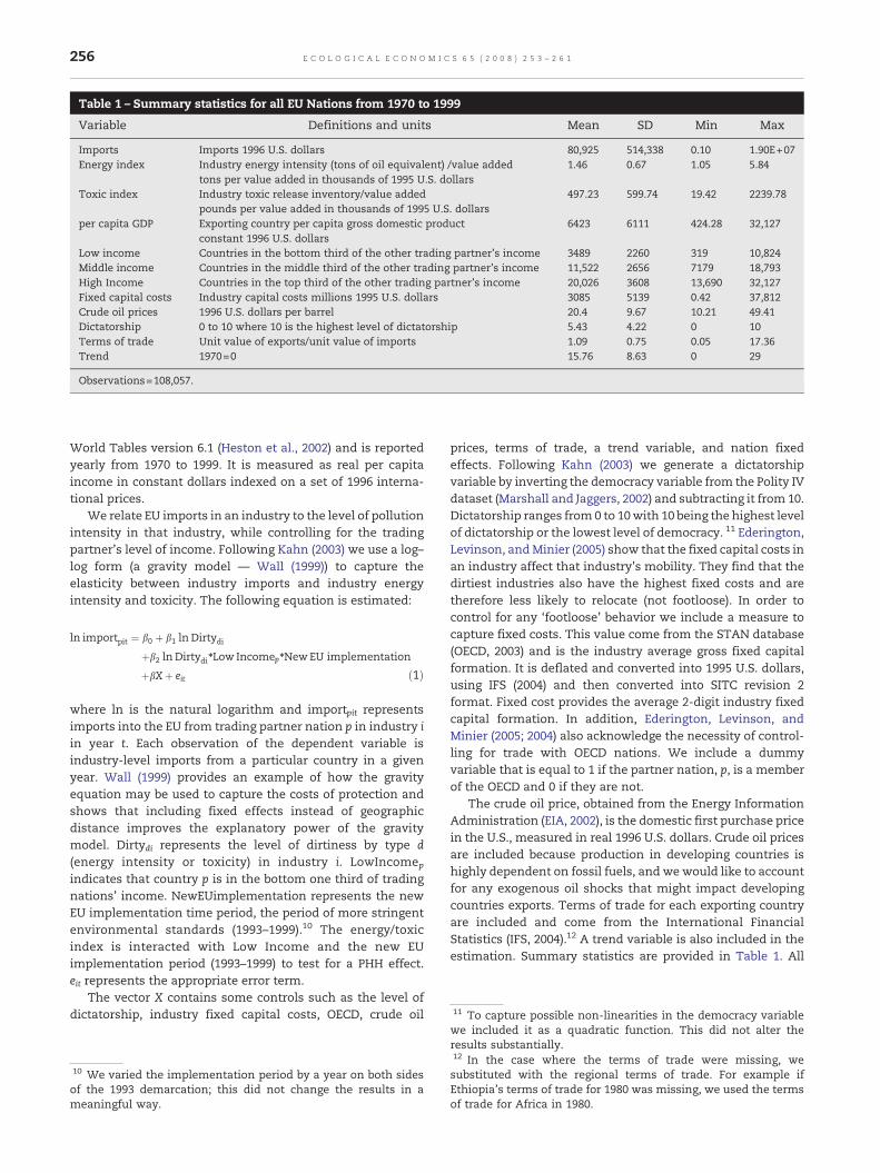
Table 1 – Summary statistics for all EU Nations from 1970 to 1999

Variable Definitions and units Mean SD Min Max

Imports Imports 1996 U.S. dollars 80,925 514,338 0.10 1.90E+07Energy index Industry energy intensity (tons of oil equivalent) /value added

tons per value added in thousands of 1995 U.S. dollars1.46 0.67 1.05 5.84

Toxic index Industry toxic release inventory/value addedpounds per value added in thousands of 1995 U.S. dollars

497.23 599.74 19.42 2239.78

per capita GDP Exporting country per capita gross domestic productconstant 1996 U.S. dollars

6423 6111 424.28 32,127

Low income Countries in the bottom third of the other trading partner's income 3489 2260 319 10,824Middle income Countries in the middle third of the other trading partner's income 11,522 2656 7179 18,793High Income Countries in the top third of the other trading partner's income 20,026 3608 13,690 32,127Fixed capital costs Industry capital costs millions 1995 U.S. dollars 3085 5139 0.42 37,812Crude oil prices 1996 U.S. dollars per barrel 20.4 9.67 10.21 49.41Dictatorship 0 to 10 where 10 is the highest level of dictatorship 5.43 4.22 0 10Terms of trade Unit value of exports/unit value of imports 1.09 0.75 0.05 17.36Trend 1970=0 15.76 8.63 0 29

Observations=108,057.

11 To capture possible non-linearities in the democracy variable

256 E C O L O G I C A L E C O N O M I C S 6 5 ( 2 0 0 8 ) 2 5 3 – 2 6 1

World Tables version 6.1 (Heston et al., 2002) and is reportedyearly from 1970 to 1999. It is measured as real per capitaincome in constant dollars indexed on a set of 1996 interna-tional prices.

We relate EU imports in an industry to the level of pollutionintensity in that industry, while controlling for the tradingpartner's level of income. Following Kahn (2003) we use a log–log form (a gravity model — Wall (1999)) to capture theelasticity between industry imports and industry energyintensity and toxicity. The following equation is estimated:

ln importpit ¼ b0 þ b1 ln Dirtydi

þb2 ln Dirtydi⁎Low Incomep⁎NewEU implementation

þbXþ eit ð1Þ

where ln is the natural logarithm and importpit representsimports into the EU from trading partner nation p in industry iin year t. Each observation of the dependent variable isindustry-level imports from a particular country in a givenyear. Wall (1999) provides an example of how the gravityequation may be used to capture the costs of protection andshows that including fixed effects instead of geographicdistance improves the explanatory power of the gravitymodel. Dirtydi represents the level of dirtiness by type d(energy intensity or toxicity) in industry i. LowIncomepindicates that country p is in the bottom one third of tradingnations' income. NewEUimplementation represents the newEU implementation time period, the period of more stringentenvironmental standards (1993–1999).10 The energy/toxicindex is interacted with Low Income and the new EUimplementation period (1993–1999) to test for a PHH effect.eit represents the appropriate error term.

The vector X contains some controls such as the level ofdictatorship, industry fixed capital costs, OECD, crude oil

10 We varied the implementation period by a year on both sidesof the 1993 demarcation; this did not change the results in ameaningful way.

prices, terms of trade, a trend variable, and nation fixedeffects. Following Kahn (2003) we generate a dictatorshipvariable by inverting the democracy variable from the Polity IVdataset (Marshall and Jaggers, 2002) and subtracting it from 10.Dictatorship ranges from 0 to 10with 10 being the highest levelof dictatorship or the lowest level of democracy. 11 Ederington,Levinson, andMinier (2005) show that the fixed capital costs inan industry affect that industry's mobility. They find that thedirtiest industries also have the highest fixed costs and aretherefore less likely to relocate (not footloose). In order tocontrol for any ‘footloose’ behavior we include a measure tocapture fixed costs. This value come from the STAN database(OECD, 2003) and is the industry average gross fixed capitalformation. It is deflated and converted into 1995 U.S. dollars,using IFS (2004) and then converted into SITC revision 2format. Fixed cost provides the average 2-digit industry fixedcapital formation. In addition, Ederington, Levinson, andMinier (2005; 2004) also acknowledge the necessity of control-ling for trade with OECD nations. We include a dummyvariable that is equal to 1 if the partner nation, p, is a memberof the OECD and 0 if they are not.

The crude oil price, obtained from the Energy InformationAdministration (EIA, 2002), is the domestic first purchase pricein the U.S., measured in real 1996 U.S. dollars. Crude oil pricesare included because production in developing countries ishighly dependent on fossil fuels, and we would like to accountfor any exogenous oil shocks that might impact developingcountries exports. Terms of trade for each exporting countryare included and come from the International FinancialStatistics (IFS, 2004).12 A trend variable is also included in theestimation. Summary statistics are provided in Table 1. All

12 In the case where the terms of trade were missing, wesubstituted with the regional terms of trade. For example ifEthiopia's terms of trade for 1980 was missing, we used the termsof trade for Africa in 1980.

we included it as a quadratic function. This did not alter theresults substantially.

257E C O L O G I C A L E C O N O M I C S 6 5 ( 2 0 0 8 ) 2 5 3 – 2 6 1

of the results are estimated using Huber–White standarderrors.13

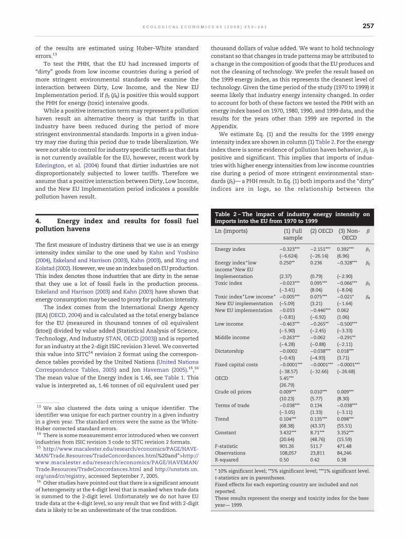
To test the PHH, that the EU had increased imports of“dirty” goods from low income countries during a period ofmore stringent environmental standards we examine theinteraction between Dirty, Low Income, and the New EUImplementation period. If β2 (β4) is positive this would supportthe PHH for energy (toxic) intensive goods.

While a positive interaction termmay represent a pollutionhaven result an alternative theory is that tariffs in thatindustry have been reduced during the period of morestringent environmental standards. Imports in a given indus-try may rise during this period due to trade liberalization. Wewere not able to control for industry specific tariffs as that datais not currently available for the EU, however, recent work byEderington, et al. (2004) found that dirtier industries are notdisproportionately subjected to lower tariffs. Therefore weassume that a positive interaction between Dirty, Low Income,and the New EU Implementation period indicates a possiblepollution haven result.

Table 2 – The impact of industry energy intensity onimports into the EU from 1970 to 1999

Ln (imports) (1) Fullsample

(2) OECD (3) Non-OECD

β

Energy index −0.323⁎⁎⁎ −2.151⁎⁎⁎ 0.392⁎⁎⁎ β1(−6.624) (−26.14) (6.96)

Energy index ⁎ lowincome ⁎New EU

0.250⁎⁎ 0.236 −0.328⁎⁎⁎ β2

Implementation (2.37) (0.79) (−2.90)Toxic index −0.023⁎⁎⁎ 0.095⁎⁎⁎ −0.066⁎⁎⁎ β3

(−3.41) (8.04) (−8.04)Toxic index ⁎Low income ⁎New EU implementation

−0.005⁎⁎⁎(−5.09)

0.075⁎⁎⁎(3.21)

−0.021⁎(−1.64)

β4

New EU implementation −0.033 −0.446⁎⁎⁎ 0.062(−0.81) (−6.92) (1.06)

Low income −0.463⁎⁎⁎ −0.265⁎⁎ −0.500⁎⁎⁎(−5.90) (−2.45) (−3.33)

Middle income −0.263⁎⁎⁎ −0.062 −0.291⁎⁎(−4.28) (−0.88) (−2.11)

Dictatorship −0.0002 −0.038⁎⁎⁎ 0.018⁎⁎⁎(−0.43) (−4.93) (3.71)

Fixed capital costs −0.0001⁎⁎⁎ −0.0001⁎⁎⁎ −0.0001⁎⁎⁎(−38.57) (−32.66) (−26.68)

OECD 5.45⁎⁎⁎(26.79)

4. Energy index and results for fossil fuelpollution havens

The first measure of industry dirtiness that we use is an energyintensity index similar to the one used by Kahn and Yoshino(2004), Eskeland and Harrison (2003), Kahn (2003), and Xing andKolstad (2002).However,weusean indexbasedonEUproduction.This index denotes those industries that are dirty in the sensethat they use a lot of fossil fuels in the production process.Eskeland and Harrison (2003) and Kahn (2003) have shown thatenergy consumptionmaybeused toproxy for pollution intensity.

The index comes from the International Energy Agency(IEA) (OECD, 2004) and is calculated as the total energy balancefor the EU (measured in thousand tonnes of oil equivalent(ktoe)) divided by value added (Statistical Analysis of Science,Technology, And Industry STAN, OECD (2003)) and is reportedfor an industry at the 2-digit ISIC revision 3 level.We convertedthis value into SITC14 revision 2 format using the correspon-dence tables provided by the United Nations (United NationsCorrespondence Tables, 2005) and Jon Haveman (2005).15,16

The mean value of the Energy index is 1.46, see Table 1. Thisvalue is interpreted as, 1.46 tonnes of oil equivalent used per

13 We also clustered the data using a unique identifier. Theidentifier was unique for each partner country in a given industryin a given year. The standard errors were the same as the White-Huber corrected standard errors.14 There is somemeasurement error introducedwhenwe convertindustries from ISIC revision 3 code to SITC revision 2 formats.15 http://www.macalester.edu/research/economics/PAGE/HAVE-MAN/Trade.Resources/TradeConcordances.html%20and">http://www.macalester.edu/research/economics/PAGE/HAVEMAN/Trade.Resources/TradeConcordances.html and http://unstats.un.org/unsd/cr/registry, accessed September 7, 2005.16 Other studies have pointed out that there is a significant amountof heterogeneity at the 4-digit level that is masked when trade datais summed to the 2-digit level. Unfortunately we do not have EUtrade data at the 4-digit level, so any result that we find with 2-digitdata is likely to be an underestimate of the true condition.

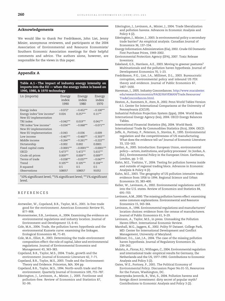
thousand dollars of value added. We want to hold technologyconstant so that changes in trade patternsmay be attributed toa change in the composition of goods that the EU produces andnot the cleaning of technology. We prefer the result based onthe 1999 energy index, as this represents the cleanest level oftechnology. Given the time period of the study (1970 to 1999) itseems likely that industry energy intensity changed. In orderto account for both of these factors we tested the PHH with anenergy index based on 1970, 1980, 1990, and 1999 data, and theresults for the years other than 1999 are reported in theAppendix.

We estimate Eq. (1) and the results for the 1999 energyintensity index are shown in column (1) Table 2. For the energyindex there is some evidence of pollution haven behavior, β2 ispositive and significant. This implies that imports of indus-tries with higher energy intensities from low income countriesrise during a period of more stringent environmental stan-dards (β2)— a PHH result. In Eq. (1) both imports and the “dirty”indices are in logs, so the relationship between the

Crude oil prices 0.009⁎⁎⁎ 0.010⁎⁎⁎ 0.009⁎⁎⁎(10.23) (5.77) (8.30)

Terms of trade −0.038⁎⁎⁎ 0.134 −0.038⁎⁎⁎(−3.05) (1.33) (−3.11)

Trend 0.104⁎⁎⁎ 0.135⁎⁎⁎ 0.098⁎⁎⁎(68.38) (43.37) (55.51)

Constant 3.432⁎⁎⁎ 8.71⁎⁎⁎ 3.352⁎⁎⁎(20.64) (48.76) (15.59)

F-statistic 901.26 511.7 471.48Observations 108,057 23,811 84,246R-squared 0.50 0.42 0.38

⁎ 10% significant level; ⁎⁎5% significant level; ⁎⁎⁎1% significant level.t-statistics are in parentheses.Fixed effects for each exporting country are included and notreported.These results represent the energy and toxicity index for the baseyear— 1999.

17 We also considered using the Industrial Pollution ProjectionSystem (IPPS) (World Bank, 2004) index. The IPPS index is the sumofthe total lower bound values of toxic pollution intensity for air,water, and land. The value is calculated with respect to the TotalValue of Output (Pounds/1987 US $ Million) and provided at the 4-digit level. AsKahn (2003) points out this index ismissing numerousindustries at the 4-digit level and probably has substantialmeasurement error. While the correlation between the TRI andIPPS index is 0.77, due to possible measurement error we decided tonot to use the IPPS index as a measure of industry dirtiness.18 Unlike the energy index we were only able to obtain the TRIindex for 1990 and 1999. The results did not vary significantlybetween the two years.

Table 3 – Summary of the results from the regional analysis

Imports (1) Non-EUEurope

(2) Africa (3) NorthAmerica

(4) Asia &Oceana

(5) Latin America &the Caribbean

β

Energy −2.158⁎⁎⁎ 0.821⁎⁎⁎ −0.475⁎⁎ −0.586⁎⁎⁎ 0.569⁎⁎⁎ β1Energy ⁎ low income ⁎New EU implementation

0.315 0.126 0.283 0.328 −0.212 β2

Toxic 0.054⁎⁎⁎ −0.029⁎⁎ 0.084⁎⁎⁎ −0.142⁎⁎⁎ −0.013 β3Toxic ⁎ low Income ⁎New EU implementation

0.032⁎ −0.045⁎ 0.069 0.033⁎ −0.094⁎⁎⁎ β4

R-squared 0.46 0.27 0.56 0.37 0.32

⁎10% significant level; ⁎⁎5% significant level; ⁎⁎⁎1% significant level.Eq. ( 1) was estimated for each region — the following variables were included and not reported: New EU implementation, low income, middleincome, dictatorship, fixed capital costs, crude oil prices, terms of trade, trend and country fixed effects— full results are available on request.

258 E C O L O G I C A L E C O N O M I C S 6 5 ( 2 0 0 8 ) 2 5 3 – 2 6 1

interactions and imports may be expressed as an elasticity. Soβ2 may be interpreted as, a 1% increase in industry energyintensity is associated with a 0.25% increase in imports fromlow income countries during the period of more stringentenvironmental standards. This evidence of an EU pollutionhaven effect for fossil fuels is fairly robust with respect to thebase year for energy technology. The point estimates for thePHH interaction coefficient are positive for all base years andstatistically significant for all but 1990.

Other results are that the EU imports fewer goods from lowincome and middle income countries relative to high incomecountries andmore goods fromOECD countries relative to non-OECD countries. The variable for fixed costs has the expectednegative sign; an increase in the average fixed cost of anindustry is associatedwith reduced EU imports in that industry.High crudeoil prices are associatedwithmore imports. Termsoftrade are negative and significant; higher prices of exportsrelative to imports are associated with reduced imports fromthat trading partner. The trend is positive and significant.

To test whether the EU is less likely to engage in “dirty” tradewith more developed countries that may have similar environ-mental standards we split the sample into non-EU OECD andnon-EU non-OECD countries and estimate Eq. (1) for each sub-sample. The results for the OECD and non-OECD countries areshown in columns (2) and (3) respectively in Table 2.

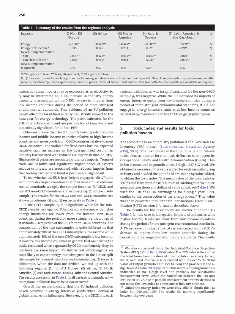
In the OECD sample, β2 is insignificant while for the non-OECDsample it is negative. EU imports of industrieswith higherenergy intensities are lower from low income, non-OECDcountries, during the period of more stringent environmentalstandards— a rejection of the PHH for non-OECDcountries. Thecomposition of the two subsamples is quite different in thatapproximately 20% of the OECD subsample is low incomewhileapproximately 80% of the non-OECD subsample is low income.It must be low income countries in general that are driving theinitial result andwhenseparated byOECDmembership, they donot have the same impact. To further test which regions aremost likely to export energy intensive goods to the EU, we splitthe sample by regional definition and estimated Eq. (1) for eachsubsample. When the data are divided, we end up with thefollowing regions: (1) non-EU Europe, (2) Africa, (3) NorthAmerica, (4) Asia andOceana, and (5) LatinandCentral America.The results are shown inTable 3. In all cases β2 is insignificant—no regional pollution haven behavior occurred.

Overall the results indicate that the EU induced pollutionhaven behavior in energy intensive goods when looking atglobal trade, i.e. the full sample.However, for theOECDandeach

regional definition β2 was insignificant, and for the non-OECDsample β2 was negative. While the EU increased its imports ofenergy intensive goods from low income countries during aperiod of more stringent environmental standards, it did notengage in energy intensive trade with low income countriesseparated by membership in the OECD or geographic region.

5. Toxic index and results for toxicpollution havens

The secondmeasure of industry pollution is the Toxic ReleaseInventory (TRI) index17 (Environmental Protection Agency(EPA), 2007). The toxic index is the total on-site and off-sitetoxic releases reported for chemicals defined as carcinogens byOccupational Safety and Health Administration (OSHA). Thisindex is measured in pounds at the 2-digit, 1987 SIC level. Weobtained ameasure of the value added for eachmanufacturingindustry and divided the pounds of emissions by value added,to obtain the toxic index. The mean value of the toxic index is497.23 and is interpreted as 497.23 lb of carcinogenic toxins aregenerated per thousand dollars of value added, see Table 1.Weused the TRI of OSHA carcinogens for a single year, 1999,similar to the construction of the energy index.18 This valuewas then converted into Standard International Trade Classi-fication (SITC) revision 2 format as described above.

The results for the toxic index are shown in column (1)Table 2. In this case β4 is negative. Imports of industries withhigher toxicity levels are lower from low income countriesduring the period of more stringent environmental standards.A 1% increase in industry toxicity is associated with a 0.005%decrease in imports from low income countries during theperiod ofmore stringent environmental standards. The results

259E C O L O G I C A L E C O N O M I C S 6 5 ( 2 0 0 8 ) 2 5 3 – 2 6 1

from the non-OECD sample are identical to the initial results.Both results are evidence against the PHH for the EU for toxicpollution.

For the OECD sample, β4 is positive and significant. Thisresult implies that the EU was more likely to import goods intoxic industries from low income OECD countries during aperiod of more stringent environmental standards — a weakPHH result. The regional results in Table 3 show that β4 isnegative for EU trade with Africa, Asia & Oceana, and Latin &Central American regions— a non-PHH result. The only regionin which the EU displayed any pollution haven behavior is fornon-EU Europe.

Overall, our results provide evidence against the PHH fortoxic pollution. For the full sample and non-OECD countriesthe coefficient for the toxic index interaction with low incomecountries during the period of more stringent EU environ-mental policy is negative and statistically significant, notpositive as we would expect if there were a pollution haveneffect. The positive sign for the toxic pollution interactionterm for EU trade within the OECD and for trade with non-EUEuropean countries provides only weak evidence in support ofthe EU fostering pollution havens in toxic pollution.

6. Discussion and conclusion

The overall results vary depending on the definition of industrydirtiness. There is evidence that the EU imported an increasedamount of energy intensive goods from poorer nations during aperiodofmore stringent environmental standards. This result isnot consistent when we break down trading partners bymembership in the OECD and regional definition. Apparentlylow income countries all together are driving the pollutionhaven effect, but that this is not a regional effect.

The results are different for toxic imports. The EU importedan increased amount of toxic goods from poorer OECDcountries during the period of more stringent environmentalstandards, but for the full sample of all trade partners thiseffect was reversed. From our study it appears that lesserdeveloped non-EU European countries or lesser developedOECD countries may have been pollution havens of toxicgoods for the EU, but overall the EU reduced its imports of toxicgoods from low income countries.

The two indices of industry dirtiness that we use providedifferent results; this is not surprising as they each measuredifferent types of pollution. Energy intensity captures thoseindustries that use a lot of fossil fuels in the production process,while industries that have high toxicitymeasures are those thatproduce significantly large amounts of carcinogens during theproduction process. The results suggest that poorer countries ingeneral have a comparative advantage in the production ofenergy intensive industries relative to similar industries in theEU, particularly when these industries are more heavilyregulated. However, this is a joint effect and does hold whenpoorer countries are divided by regional definition and OECDmembership.

The opposite is true for highly toxic industries. Once theseindustries become more heavily regulated within the EU,poorer OECD countries gain a comparative advantage in theproduction and export of these industries and we observe

increased toxic trade between the EU and poorer non-EUEuropean/OECD countries. This effect only holds for poorerOECD and non-EU European countries. In general we find thatwhen toxic industries became more heavily regulated withinthe EU, this did not affect domestic industries comparativeadvantage and the EU reduced its imports of toxic goods frompoorer countries in general.

There are some caveats to our results that should be con-sidered. First we use a toxicity index based on U.S. technology.The toxic index represents ameasure of industry toxicity basedon 1999 U.S. technology, and the energy index captures thecleanness of EU technology in 1999. Table 1 in the Appendixdisplays a summary of the resultswhenwe use an energy indexbased on 1970, 1980, and 1990 technology. For energy intensity,we observe a pollution haven result in all cases although thecoefficient for 1990 is not statistically significant. By choosing1999 as our base year for technology we are using the cleanesttechnology and may mask potential pollution haven behavior.

A case can be made that our estimates of the effect ofstringency of EU environmental policy on the pollution inten-sity of imports is too low. Previous studies have found thatsignificant variation in pollution intensity between 4-digitindustries exists within a 2-digit industry specifica-tion (Levinson and Taylor (forthcoming); Ederington, et al.(2005); Ederington andMinier (2003); Kahn (2003)). These studiesshow that by aggregating production to the 2-digit level, we areunderestimating the pollution haven effect, resulting in adownward bias of the results. If we had been able to estimatethe import equation with industries that are more narrowlydefined, we probably would have found stronger impacts.

Another factor that may mask a pollution haven effect isthat we ignore the pollution content of intermediate goods.The EUmay change the composition of goods that it produces.Instead of producing a final good that requires importing adirty intermediate good, the EU imports the final good. Thischange in behavior will appear to be a reduction in the importsof dirty goods, although the EU may still be consuming thesame number of final goods. An additional factor that maymask pollution haven behavior is increasing energy intensi-ties in developing countries. If developing countries havebecome more energy intensive over time this will driveproduction costs up and these countries will be unable toproduce and export as many energy intensive goods as before.This change in trade would appear as a reduction in energyintensity trade when in fact that is not the case.

Future work will try to reexamine this question using moredisaggregated data. In addition there are some interestingpolicy issues to consider, in particular the impact of increasedcommunity wide environmental stringency on EU enlarge-ment. The ten countries that are new EU entrants in 2004 areheterogeneous jurisdictions that are fairly new to the demo-cratic process. These countries are likely to focus on increas-ing their income as they become integrated into the EU. Theincoming countries tend to be less developed than the EU andit is likely that it will have a comparative advantage in theproduction of dirty goods. Overall EU entrants may beresistant to strict uniform enforcement of environmentalregulations. The fact that the EU imports dirty goods fromnew entrants may have some interesting implications asenlargement and integration continues.

260 E C O L O G I C A L E C O N O M I C S 6 5 ( 2 0 0 8 ) 2 5 3 – 2 6 1

Acknowledgements

We would like to thank Per Fredriksson, John List, JennyMinier, anonymous reviewers, and participants at the 2004Association of Environmental and Resource Economists/Southern Economic Association meetings for their helpfulcomments and advice. The authors alone, however, areresponsible for the views in this paper.

Appendix A

Table A.1 – The impact of industry energy intensity onimports into the EU — when the energy index is based on1990, 1980, & 1970 technology

Ln (imports) Energyindex1990

Energyindex1980

Energyindex1970

Energy index −0.072⁎ −0.452⁎⁎⁎ −0.100⁎⁎⁎Energy index ⁎ low income⁎New EU implementation

0.024 0.257⁎⁎⁎ 0.11⁎⁎⁎

TRI index −0.042⁎⁎⁎ 0.019⁎⁎⁎ 0.041⁎⁎⁎TRI index ⁎ low income ⁎New EU implementation

−0.034⁎⁎⁎ −0.068⁎⁎⁎ −0.071⁎⁎⁎

New EU implementation −0.043 −0.036 −0.009Low income −0.467⁎⁎⁎ −0.460⁎⁎⁎ −0.393⁎⁎⁎Middle income −0.264⁎⁎⁎ −0.261⁎⁎⁎ −0.222⁎⁎⁎Dictatorship −0.002 0.002 0.0001Fixed capital costs −0.0001⁎⁎⁎ −0.0001⁎⁎⁎ −0.0001⁎⁎⁎OECD 5.473⁎⁎⁎ 5.472⁎⁎⁎ 5.615⁎⁎⁎Crude oil prices 0.009⁎⁎⁎ 0.009⁎⁎⁎ 0.009⁎⁎⁎Terms of trade −0.038⁎⁎⁎ −0.037⁎⁎⁎ −0.047⁎⁎⁎Trend 0.105⁎⁎⁎ 0.105⁎⁎⁎ 0.104⁎⁎⁎R-squared 0.5 0.5 0.5Observations 108057 108057 91052

⁎10% significant level; ⁎⁎5% significant level; ⁎⁎⁎1% significantlevel.

R E F E R E N C E S

Antweiler, W., Copeland, B.R., Taylor, M.S., 2001. Is free tradegood for the environment. American Economic Review 91,877–908.

Brunnermeier, S.B., Levinson, A., 2004. Examining the evidence onenvironmental regulations and industry location. Journal ofEnvironment and Development 13, 6–41.

Cole, M.A., 2004. Trade, the pollution haven hypothesis and theenvironmental Kuznets curve: examining the linkages.Ecological Economics 48, 71–81.

Cole, M.A., Elliot, R., 2003. Determining the trade–environmentcomposition effect: the role of capital, labor and environmentalregulations. Journal of Environmental Economics andManagement 43, 363–383.

Copeland, B.R., Taylor, M.S., 2004. Trade, growth and theenvironment. Journal of Economic Literature 42, 7–71.

Copeland, B.R., Taylor, M.S., 2003. Trade and the Environment:Theory and Evidence. Princeton, MA. 304 pp.

Copeland, B.R., Taylor, M.S., 1994. North–south trade and theenvironment. Quarterly Journal of Economics 109, 755–787.

Ederington, J., Levinson, A., Minier, J., 2005. Footloose andpollution-free. Review of Economics and Statistics 87,92–99.

Ederington, J., Levinson, A., Minier, J., 2004. Trade liberalizationand pollution havens. Advances in Economic Analysis andPolicy 4 (2).

Ederington, J., Minier, J., 2003. Is environmental policy a secondarytrade barrier? An empirical analysis. Canadian Journal ofEconomics 36, 137–154.

Energy Information Administration (Eia), 2002. Crude Oil DomesticFirst Purchase Prices, 1949–2002.

Environmental Protection Agency (EPA), 2007. Toxic ReleaseInventory.

Eskeland, G.S., Harrison, A.E., 2003. Moving to greener pastures?Multinationals and the pollution haven hypothesis. Journal ofDevelopment Economics 70, 1–23.

Fredriksson, P.G., List, J.A., Millimet, D.L., 2003. Bureaucraticcorruption, environmental policy and inbound US FDI:theory and evidence. Journal of Public Economics 87,1407–1430.

Haveman, J., 2005. Industry Concordances. http://www.macalester.edu/research/economics/PAGE/HAVEMAN/Trade.Resources/TradeConcordances.html.

Heston, A., Summers, R., Aten, B., 2002. PennWorld Tables Version6.1. Center for International Comparisons at the University ofPennsylvania (CICUP).

Industrial Pollution Projection System (Ipps), 2004. World Bank.International Energy Agency (Iea), 2004. OECD Energy Balances

Tables.International Financial Statistics (Ifs), 2004. World Bank.International Trade By Commodities Statistics (Itcs), 2004. OECD.Jaffe, A., Portney, P., Peterson, S., Stavins, R., 1995. Environmental

regulation and the competitiveness of US manufacturing.What does the evidence tell us? Journal of Economic Literature33, 132–163.

Jordan, A., 2005. Introduction: European Union, environmentalpolicy— actors, institutions, andpolicy processes'. In: Jordan, A.(Ed.), Environmental Policy in the European Union. Earthscan,London, pp. 1–10.

Kahn, M.E., Yoshino, Y., 2004. Testing for pollution havens insideand outside of regional trading blocs. Advances in EconomicAnalysis & Policy 4 (2).

Kahn, M.E., 2003. The geography of US pollution intensive trade:evidence from 1958 to 1994. Regional Science and UrbanEconomics 33, 383–400.

Keller, W., Levinson, A., 2002. Environmental regulations and FDIinto the U.S. states. Review of Economics and Statistics 84,691–703.

Levinson, A.M., 2000. Themissing pollutionhaven effect: examiningsome common explanations. Environmental and ResourceEconomics 15, 343–364.

Levinson, A., 1996. Environmental regulations andmanufacturers'location choices: evidence from the census of manufacturers.Journal of Public Economics 61, 9–29.

Levinson, A., Taylor, M.S., in press. Unmasking the PollutionHaven Effect. International Economic Review.

Marshall, M.G., Jaggers, K., 2002. Polity IV Dataset. College Park,MD: Center for International Development and ConflictManagement, University of Maryland.

Millimet, D.L., List, J.A., 2004. The case of the missing pollutionhaven hypothesis. Journal of Regulatory Economics 26,239–262.

Mulatu, A., Florax, R.J.,Withagen, C., 2004. Environmental regulationand international trade: empirical results for Germany, theNetherlands and the US, 1977–1992. Contributions to EconomicAnalysis and Policy 3 (2).

Oates, W.E., Portney, P., 2001. The Political Economy ofEnvironmental Policy. Discussion Paper No.01-55, Resourcesfor the Future, Washington, DC.

Smarzynska Javorcik, B., Wei, S., 2004. Pollution havens andforeign direct investment: dirty secret of popular myth?Contributions to Economic Analysis and Policy 3 (2).

261E C O L O G I C A L E C O N O M I C S 6 5 ( 2 0 0 8 ) 2 5 3 – 2 6 1

Statistical Analysis Of Science, Technology And Industry (Stan),2003. Oecd.

The Kyoto Protocol And Climate Change, 2005.United Nations Correspondence Tables, 2005.Wall, H.J., 1999. Using the gravity model to estimate the costs of

protection. Federal Reserve Bank of St. Louis Review., January/February 33–40.

Wilkinson, D., 2002. Maastricht and the environment: theimplications for the EC's \ environmental policy of the treatyon European Union. In: Jordan, A. (Ed.), Environmental Policy inthe European Union. Earthscan, London, pp. 37–52.

Xing, Y., Kolstad, C.D., 2002. Do lax environmental regulationsattract foreign investment. Environmental and ResourceEconomics 21 (1), 1–22.