environmental effects of agricultural land-use...
TRANSCRIPT
Environmental Effects ofAgricultural Land-Use Change
United StatesDepartment ofAgriculture
Ruben N. Lubowski, Shawn Bucholtz, Roger Claassen,Michael J. Roberts, Joseph C. Cooper, Anna Gueorguieva,and Robert Johansson
EconomicResearchService
EconomicResearchReportNumber 25 The Role of Economics and Policy

United StatesDepartmentof Agriculture
www.ers.usda.gov
A Report from the Economic Research Service
Economic
Research
Report
Number 25 Environmental Effects ofAgricultural Land-Use Change
The Role of Economics and Policy
Ruben N. Lubowski, Shawn Bucholtz, RogerClaassen, Michael J. Roberts, Joseph C. Cooper,Anna Gueorguieva, and Robert Johansson
August 2006
Abstract
This report examines evidence on the relationship between agricultural land-usechanges, soil productivity, and indicators of environmental sensitivity. If cropland thatshifts in and out of production is less productive and more environmentally sensitivethan other cropland, policy-induced changes in land use could have production effectsthat are smaller—and environmental impacts that are greater—than anticipated. To illus-trate this possibility, this report examines environmental outcomes stemming from land-use conversion caused by two agricultural programs that others have identified aspotentially having important influences on land use and environmental quality: Federalcrop insurance subsidies and the Conservation Reserve Program (CRP), the Nation’slargest cropland retirement program. The report finds that lands moving between culti-vated cropland and less intensive agricultural uses are, on average, less productive andmore vulnerable to erosion than other cultivated lands, both nationally and locally.These lands are also associated with greater potential nutrient runoff and leachingcompared with cultivated cropland nationally. Crop insurance subsidies and CRP haveestimated effects on erosion and other environmental factors that are disproportionate tothe acreage and production effects, but specific environmental impacts vary with thefeatures of each program.
Keywords: Conservation Reserve Program (CRP), crop insurance, erosion, extensivemargin, farm policy, imperiled species, land use, land-use change, land quality, nutrientloss, soil productivity.

Acknowledgements
The authors thank Mary Bohman, Daniel Hellerstein, Utpal Vasavada, KeithWiebe, and Marca Weinberg for helpful comments on earlier drafts of thisreport. We are grateful to Barry Goodwin from North Carolina State Univer-sity; John Horowitz from the University of Maryland; Mark Schwartz fromU.C. Davis; Rich Iovanna, Skip Hyberg, and Alexander Barbarika from theUSDA Farm Service Agency (FSA); and Thomas Worth from the USDARisk Management Agency (RMA) for thoughtful reviews. We thank BrianGross and Kent Kovacs for excellent research assistance. We also thankDale Simms for editorial assistance and Wynnice Pointer-Napper forgraphics and layout.
iiEnvironmental Effects of Agricultural Land-Use Changes / ERR-25
Economic Research Service/USDA

Contents
Summary . . . . . . . . . . . . . . . . . . . . . . . . . . . . . . . . . . . . . . . . . . . . . . . . . . .iv
Chapter 1Agricultural Policy and Environmental Effects of Marginal Cropland Changes . . . . . . . . . . . . . . . . . . . . . . . . . . . . . . . . . .1
Economics of Land-Use Change . . . . . . . . . . . . . . . . . . . . . . . . . . . . . . .3Environmental Characteristics of Transitioning Lands . . . . . . . . . . . . . .3Impacts of Federal Agricultural Policies: Crop Insurance and the
Conservation Reserve Program . . . . . . . . . . . . . . . . . . . . . . . . . . . . . . .4
Chapter 2The Extensive Margin of Cultivated Cropland . . . . . . . . . . . . . . . . . . . .6
Historical Changes in Total Cropland Used for Crops . . . . . . . . . . . . . . .6Land-Use Changes at the Extensive Margin of Cropland, 1982-97 . . . .7The Extensive Margin of Cultivated Cropland Is Not Equally
Active in All Regions . . . . . . . . . . . . . . . . . . . . . . . . . . . . . . . . . . . . .11
Chapter 3Land Quality and Land-Use Change . . . . . . . . . . . . . . . . . . . . . . . . . . . .17
A Model of Land Allocation and Land Quality . . . . . . . . . . . . . . . . . . .18Economic Characteristics of Transitioning Lands . . . . . . . . . . . . . . . . . .22Conclusion . . . . . . . . . . . . . . . . . . . . . . . . . . . . . . . . . . . . . . . . . . . . . . . . .
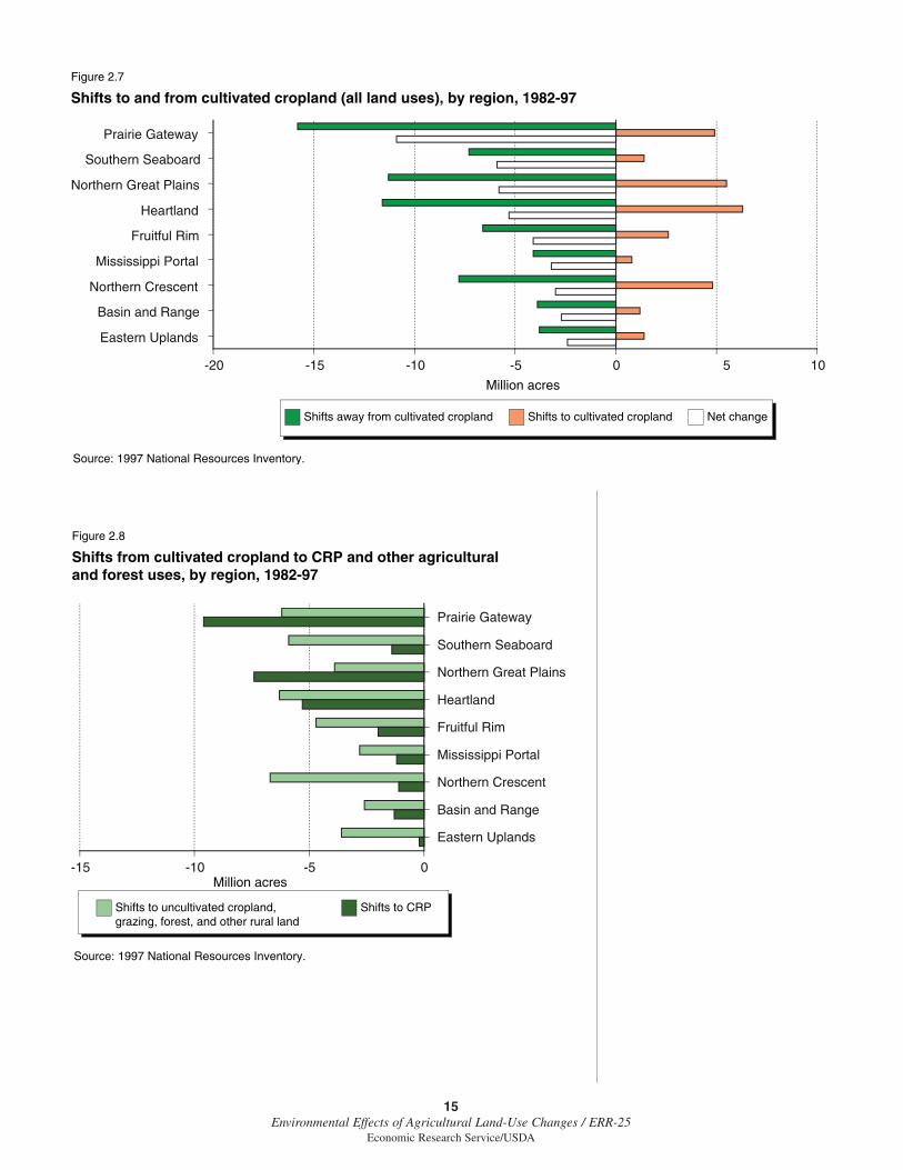
Chapter 4Environmental Characteristics of Economically Marginal Cropland . . .26
Lands With Low Soil Productivity are More Vulnerable to Erosion Damage . . . . . . . . . . . . . . . . . . . . . . . . . . . . . .26
Soil Productivity And Nutrient Losses . . . . . . . . . . . . . . . . . . . . . . . . . .27Cropland That Converted to Other Uses Was More Prone to
Erosion Damage and Nutrient Loss . . . . . . . . . . . . . . . . . . . . . . . . . .31Lands Moving In and Out of Cultivation Generally Associated
with More Imperiled Species . . . . . . . . . . . . . . . . . . . . . . . . . . . . . . .36Conclusion . . . . . . . . . . . . . . . . . . . . . . . . . . . . . . . . . . . . . . . . . . . . . . . . .
Chapter 5Environmental Effects of Policy-Induced Land-Use Changes . . . . . . .43
Analytical Model: The Effect of Crop Insurance Subsidies on Land-Use Change . . . . . . . . . . . . . . . . . . . . . . . . . . . . . . . . . . . . . .44
Higher Insurance Subsidies Increased 1997 Cropland Acreage by Up to 1 Percent . . . . . . . . . . . . . . . . . . . . . . . . . . . . . . . . . . . . . . .46
Crop Insurance Has a Disproportionate Impact on Low Quality and Certain Environmentally Sensitive Land . . . . . . . . . . . . . . . . . . .47
Lands Affected by Crop Insurance Subsidies and Imperiled Species Habitat . . . . . . . . . . . . . . . . . . . . . . . . . . . . . . . . . . . . . . . . . .51
Crop Insurance Effects on Wind and Water Erosion . . . . . . . . . . . . . . .51
Conclusions . . . . . . . . . . . . . . . . . . . . . . . . . . . . . . . . . . . . . . . . . . . . . . . . .53
References . . . . . . . . . . . . . . . . . . . . . . . . . . . . . . . . . . . . . . . . . . . . . . . . . .54
Appendix A: Land-Use Data . . . . . . . . . . . . . . . . . . . . . . . . . . . . . . . . . .61Appendix B: EPIC-Based Nutrient Loss Indicators . . . . . . . . . . . . . . .63Appendix C: Imperiled Species Counts . . . . . . . . . . . . . . . . . . . . . . . . .66Appendix D: Estimating Land-Use Changes From Crop
Insurance Subsidies . . . . . . . . . . . . . . . . . . . . . . . . . . . . . . . . . . . . . . .67Appendix E: Estimating Erosion From Policy-Driven
Changes in Land Use . . . . . . . . . . . . . . . . . . . . . . . . . . . . . . . . . . . . . .75
iiiEnvironmental Effects of Agricultural Land-Use Changes / ERR-25
Economic Research Service/USDA

Summary
While total U.S. cropland has remained roughly constant for 100 years,this stability belies larger underlying movements of land into and out ofcrop production. Almost three-quarters of the cropland that shifted into orout of cultivation between 1982 and 1997 had soil productivity ratingsbelow the average acre of cropland. Farmers tend to keep highly produc-tive cropland in cultivation regardless of changing economic conditions.But economic conditions, such as changing commodity prices or produc-tion costs, encourage farmers to expand production to less productive landor to shift less productive croplands to other uses. Agricultural and conser-vation policies also affect land use. These land use changes affect environ-mental quality, particularly when affected lower-quality lands areenvironmentally sensitive.
What Is the Issue?
Although many have speculated that less productive croplands are moreenvironmentally sensitive, little empirical evidence is available to substan-tiate this idea. If cropland that shifts in and out of production is less produc-tive and more environmentally sensitive than other cropland, policy-inducedchanges in land use could have production economic effects that aresmaller—and environmental impacts that are greater—than anticipated.
This report examines how the attributes of lands shifting into and out ofcrop production differ from those of continuously cultivated cropland. Wefocus particularly on cropland change affected by the Conservation ReserveProgram (CRP) and Federal crop insurance, government programs thatothers have identified as potentially having important influences on land useand environmental quality. Since 1985, CRP has been the largest driver ofcropland changes. This land retirement program pays farmers to retire crop-land acreage to achieve environmental goals. In 2005, the CRP paid farmers$1.7 billion to retire a land area almost the size of Iowa. Due to its competi-tive bidding process and selection criteria, CRP enrolls land that is lessproductive and more environmentally sensitive than average cropland. TheFederal crop insurance program, on the other hand, raises incentives toexpand crops to less productive land. Environmental groups, economists,and others have expressed concern that this may induce cultivation infrequently flooded and other risky areas containing wetlands or other envi-ronmentally sensitive lands.
What Did the Study Find?
Between 1982 and 1997, there was a net decline in cultivated cropland of 43million acres (11 percent). Over the same time, more than 127 million acresor 32 percent of cultivated cropland shifted between cultivated cropland andless intensive uses. These shifting lands are generally less productive thancontinuously cultivated croplands.
On average, land shifting in and out of cultivation is more vulnerable toerosion (from rainfall and often wind) and—except for CRP acreage—hasgreater nutrient runoff and leaching potential than more productive crop-
ivEnvironmental Effects of Agricultural Land-Use Changes / ERR-25
Economic Research Service/USDA

land. While these nutrient loss estimates take into account land erodibility,they may not accurately reflect differences in fertilizer applications on lowerproductivity lands.
Lands enrolling in CRP are generally less productive than other landsshifting into and out of crop production. On average, CRP acres (if returnedto cultivation) would be more vulnerable to erosion, but do not have higherpotential nutrient runoff and leaching to water, than other cropland areas.The 8-percent reduction in cultivated cropland area attributed to CRPreduced aggregate wind and water erosion by an estimated 16 and 7 percentannually, as of 1997.
Increased crop insurance subsidies in the mid-1990s motivated farmers toexpand cultivated cropland area in the contiguous 48 States by an estimated2.5 million acres (0.8 percent) in 1997, with the bulk of this land comingfrom hay and pasture. This land-use change increased annual wind andwater erosion by an estimated 1.4 and 0.9 percent, as of 1997.
Lands brought into or retained in cultivation due to these crop insurancesubsidy increases are, on average, less productive, more vulnerable to erosion,and more likely to include wetlands and imperiled species habitats, than culti-vated cropland overall. Based on nutrient application data, these lands are alsoassociated with higher levels of potential nutrient losses per acre.
Lands shifting in and out of cultivation are generally located in areas withmore imperiled plant and vertebrate species than cropland persisting incultivation. Lands in cultivation due to increased insurance subsidies tend tolie in watersheds with higher average counts of imperiled vertebrate, plant,and fish/mollusk species, relative to cultivated cropland overall. CRP landsare in areas with greater average counts of imperiled birds but not of otherimperiled species examined. (Our species indicator is the number of speciesconsidered imperiled throughout their range from NatureServe's NaturalHeritage data. Although these data are the most comprehensive measure ofU.S. biodiversity conservation status, the available data are insufficient todetermine whether the associated changes in land use have an impact—either positive or negative—on imperiled species.)
These results suggest that policies that increase incentives for crop cultiva-tion and stimulate production on economically marginal land may havedisproportionately large unintended environmental consequences.Conversely, large environmental benefits could be achieved at lower costusing targeted conservation programs because owners of low-quality andenvironmentally sensitive land require less payment to remove land fromproduction than owners of higher-quality land.
How Was the Study Conducted?
Historical patterns of land-use change are examined to establish relation-ships between land quality and land use. This report also estimates land-use and environmental impacts stemming from two government programsthat may affect less productive and environmentally sensitive croplands:federally subsidized crop insurance and the CRP.
vEnvironmental Effects of Agricultural Land-Use Changes / ERR-25
Economic Research Service/USDA

The report compares the economic and environmental characteristics oflands that persist in cultivation and those that have recently shifted betweencultivated cropland and other, less intensive, uses such as hay, forest,pasture, range, and CRP. These are lands on which uses actually have beenaffected by recent economic changes or other factors. Using parcel-leveldata on land use and land characteristics from USDA's National ResourcesInventory (NRI), the report examines associations between measures ofagricultural productivity, enrollment in CRP and other land-use changes,and environmental factors including rainfall and wind erosion; potentialnutrient losses reaching groundwater, surface water, and estuaries; and loca-tion relative to imperiled species habitat.
While lands in CRP are analyzed directly, we estimate the extent, location,and characteristics of lands cropped due to insurance subsidies through astatistical analysis of land-use changes surrounding the large increase incrop insurance subsidies after the 1994 Crop Insurance Reform Act. Thereport compares land-use changes between 1992 and 1997 given differentincreases in the expected gains from the newly increased subsidies.
viEnvironmental Effects of Agricultural Land-Use Changes / ERR-25
Economic Research Service/USDA

Environmental groups, ecologists, economists, and others have expressedconcern that agricultural programs that stimulate production can have unin-tended and undesired environmental consequences. This view is based ontwo ideas: first, that as more land is used in agricultural production, lessland remains for wildlife or other environmental purposes; and second, thatless productive agricultural lands are particularly susceptible to environ-mental damages. This report examines both ideas, but focuses mainly on thesecond one, in the context of agricultural production in the United States.
While the loss of forests and other areas to crop production may be criticalin developing countries with expanding cropland areas, the amount of landused for U.S. crop production has remained relatively stable for the last 100years. The use of particular lands in the United States has changed overtime, however, with some cropland converted to urban, forest, and otheruses, and some forests, pasture, and range switching to cropland. Littleinformation exists on the environmental implications of these land-use tran-sitions and the degree to which policies may be affecting them. If croplandthat shifts in and out of production is less productive and more environmen-tally sensitive than other cropland, policy-induced changes in land use couldhave production effects that are smaller—and environmental impacts thatare greater—than anticipated.
The view that economically marginal lands are environmentally fragile drawson basic economic and agronomic principles. For example, all else being thesame, highly sloped lands are more erodible and may be more difficult tocultivate. Some also argue that poorer soils require greater nutrient applica-tions if engaged in intensive agricultural uses, which may cause greaternutrient runoff depending on application methods and levels, rainfall runoff,soil erosion, and other factors. Thus, it makes sense that some environmen-tally fragile lands would be near the economic margin between cropland andless intensive agricultural uses, such as pasture. These marginal lands could bemore likely to shift uses due to changes in governmental policies, commodityprices, or production costs. Thus, crop insurance subsidies, income supportprograms, and other government programs that may stimulate agriculturalproduction could harm the environment more than the change in croplandacres would suggest. Conversely, large environmental benefits could beachieved at lower cost using targeted conservation programs because ownersof low-quality and environmentally sensitive land might require less paymentto remove land from production than would owners of higher quality land.
Although there is some logic to this view, little empirical evidence exists on therelationships between soil productivity and environmental sensitivity. More-
1Environmental Effects of Agricultural Land-Use Changes / ERR-25
Economic Research Service/USDA
Chapter 1
Agricultural Policy andEnvironmental Effects of
Marginal Cropland Changes

over, there are surely exceptions. In southeast Washington, for example, deepfertile soil in the rolling (erodible) hills of the Palouse Country supports muchof the State’s wheat farming (Pimentel and Kounang, 1998). Even the broaderenvironmental implications of erodibility are unclear. For example, if highlyerodible lands lie farther from waterways, sediment and nutrient runoff fromagricultural activities on these lands may cause less offsite damage.
Whether or not the link between land quality and environmental sensitivityis valid, it emphasizes the importance of examining economic and environ-mental factors jointly. The view that government farm policies that stimulateproduction are particularly damaging to the environment hinges on thefollowing three logical premises:
(1) Economic forces are likely to cause lower quality land to transitioninto and out of crop production.
(2) Lower quality croplands are more environmentally sensitive.
(3) Agricultural policies affect land use on these low-quality and environ-mentally sensitive lands at the economic margin of crop production.
By exploring each of these assumptions, we begin to trace out the linksbetween agricultural policy, land use, and its environmental consequences (fig.1.1). External forces—such as food and fiber demand, technology, and indi-
2Environmental Effects of Agricultural Land-Use Changes / ERR-25
Economic Research Service/USDA
External FactorsFood demand
Individual preferencesTrade lawsTechnology
Agricultural PolicyCrop insurance
Commodity programsCRPEQIP
Land AttributesSoil type
SlopeLocationClimate
Land Use and Management
Extensive Margin
Broad land-usechoices (e.g. crops,pasture, forest)
Intensive Margin
Crop choicePesticide useStocking rateTillage practicesMitigation efforts
Market ResponsesCommodity prices
Input pricesOrganizational structure
Environmental OutcomesErosionWildlife
Water quality
FEEDBACK
Tracing the links between policy, land use, and the environmentFigure 1.1
vidual producer preferences—together with agricultural policy and land attrib-utes, directly affect incentives pertaining to land use and land management.
Land use and management influence the supply of agricultural commodities,and thus their prices and the organizational structure of U.S. agriculture.These market outcomes, in turn, influence land use. The land uses thatculminate from these forces interact with land attributes to determine envi-ronmental outcomes. Our objective is to trace out some of these links.
Economics of Land-Use Change
Historical patterns of land-use change can be used to more firmly establishrelationships between land quality and land use. Lands that have recentlyshifted into or out of cultivated cropland from other, less intensive uses areat the extensive margin of cultivated land, with land use evidently suscep-tible to economic or other forces (see box, “The Extensive and IntensiveMargins of Cropland Use”). One may compare land attributes (such as yieldpotential, slope, and location) of transitioning lands and lands that have notshifted to a different land use to infer economic forces driving land-usechange and whether transitioning lands are of lower quality.
There can be many extensive margins, including land straddling crop andpasture uses and land straddling crop and forest uses.1 Although landmoving from agricultural to urban uses is a prominent issue near somemetropolitan areas, this is a small area nationally because urban areascomprise such a small share of total land use in the United States. Between1982 and 1997, transitions from cultivated cropland to urban land occurredon just 1.5 percent of cultivated cropland.2 By comparison, transitions tohay, Conservation Reserve Program (CRP), and “other” uses (pasture,range, and forest) occurred on over 24 percent of cultivated cropland. Landsthat shifted into crop cultivation from these less intensive uses during 1982-97 constituted 9 percent of cultivated cropland in 1997 (USDA/NRCS,2000). Because urban land uses are so valuable relative to agricultural useson some lands, these transitions are driven by factors considerably differentfrom those that drive transitions between intensive and less intensive agri-cultural uses. Agricultural-to-urban transitions are also less likely to beinfluenced by Federal agricultural policies.3
Environmental Characteristics ofTransitioning Lands
Are lands of low agricultural value also more likely to move into and out ofintensive agricultural uses, and are they more susceptible to environmentaldamages? Comparing various measures of environmental sensitivity (erosion,nutrient leaching/runoff, and encroachment on species habitat) on low-qualityor recently transitioning lands versus higher quality or nontransitioning landsindicates whether the former are more prone to certain environmental damages.Quantifying these differences suggests the environmental consequences of thevarious economic forces that drive land-use change.
This report seeks to illustrate the environmental outcomes stemming fromextensive margin choices. Intensive margin choices, however, are made
1In keeping with common usage ineconomics, we use the term “extensivemargin” to refer generically to the eco-nomic margin between any two land-use alternatives. With respect tocropland uses, changes at the extensivemargin can be defined in terms of broadland-use categories, as in this report, ormore specifically in terms of specificcrops (e.g., Wu, 1999). Other authors(Barlowe, 1958) use the term “extensivemargin” to refer only to the economicmargin beyond which all land usescease to provide economic rents andland is left abandoned or unused.
2Urban land use is defined in accor-dance with the definition given byUSDA’s National Resources Inventory(NRI) as: “A land cover/use categoryconsisting of residential, industrial,commercial, and institutional land; con-struction sites; public administrativesites; railroad yards; cemeteries; air-ports; golf courses; sanitary landfills;sewage treatment plants; water controlstructures and spillways; other land usedfor such purposes; small parks (less than10 acres) within urban and built-upareas; and highways, railroads, andother transportation facilities if they aresurrounded by urban areas. Alsoincluded are tracts of less than 10 acresthat do not meet the above definition butare completely surrounded by urban andbuilt-up land.”
3With the exception of the USDAFarm and Ranch Lands ProtectionProgram, which funds purchases ofdevelopment rights on agriculturallands, Federal agricultural policies areunlikely to influence land-use change atthe agricultural-urban fringe. Otherresearchers have examined local zoninglaws and other factors affecting urban-ization of agricultural land (Carrion-Flores and Irwin, 2004; Irwin et al.,2003; Heimlich and Anderson, 2001;Bockstael, 1996).
3Environmental Effects of Agricultural Land-Use Changes / ERR-25
Economic Research Service/USDA

simultaneously with extensive margin choices (see box, “The Extensive andIntensive Margins of Cropland Use”). Ideally, we would consider both setsof choices simultaneously, but the complexity of the modeling and datarequirements make such an analysis infeasible. Because the environmentaleffects of broad land-use changes induced by policy have received littleempirical attention, we focus on extensive margin changes, while drawingon assumptions about intensive margin choices that are based on moreaggregated data and pre-existing models.4
Impacts of Federal Agricultural Policies:Crop Insurance and the ConservationReserve Program
In addition to broadly examining relationships between soil productivity, envi-ronmental sensitivity, and land-use change, this report examines environmentaloutcomes stemming from land-use conversion caused by specific agriculturalprograms that may have particular relevance for lower quality land.Researchers have noted the potential for farm programs to generate unintendednegative environmental consequences by increasing the amount of cultivatedcropland (e.g., Goodwin and Smith, 2003; Wu, 1999; Plantinga, 1996). Manyagricultural policies have been cited as encouraging producers to cultivate addi-tional land or retain land in cultivation when it would not otherwise be prof-itable to do so. These studies include land-use effects of commodity programs(e.g., Plantinga, 1996; Wu and Segerson, 1995; Wu and Brorsen, 1995),acreage effects of crop insurance subsidies (Goodwin et al., 2004; Deal, 2004;Goodwin et al., 1999; Griffin, 1996; Keeton et al., 1999; Wu, 1999; Young etal., 1999), and disaster payments (Gardner and Kramer, 1986). A few studieshave also analyzed the environmental effects of these changes (Deal, 2004;Goodwin and Smith, 2003; Wu, 1999; Plantinga, 1996). These studies,however, have mainly examined environmental outcomes for particular regions,not for the Nation as a whole.
4Environmental Effects of Agricultural Land-Use Changes / ERR-25
Economic Research Service/USDA
Lands near the economic margin of two or more competing uses lie on theextensive margin of the higher value use. Changes in broad categories ofland use, including movements of land into and out of crop production, aretermed extensive margin choices. Intensive margin choices refer to theparticular crop choices (e.g., corn versus soybeans) and crop-specific appli-cation rates of inputs such as pesticides, water, and fertilizer. In otherwords, the difference between extensive and intensive choices refers to thedifference between how the land is used in a general sense and how it ismanaged more specifically. This report focuses on the economics and envi-ronmental implications of changes in the use of land for crop cultivationversus other less intensive uses and on the role of agricultural policies ininfluencing these extensive margin choices. Other research has examinedpolicy impacts on crop choices and input use and the associated environ-mental consequences (Babcock and Hennessy, 1996; Smith and Goodwin,1996; Wu and Brorsen, 1995; Wu and Segerson, 1995; Horowitz and Licht-enberg, 1993; Quiggin et al., 1993).
The Extensive and Intensive Margins of Cropland Use
4We generate environmental indica-tors for nutrient runoff and leachingusing the Environmental PolicyIntegrated Climate Model (EPIC), acrop biophysical simulation model thatestimates the impact of managementpractices on crop yields, soil quality,and various environmental emissions atthe field level (Mitchell et al., 1998).

Environmental outcomes depend on the magnitude of land-use changesinduced by policies and on land attributes of affected versus nonaffectedparcels. We focus on two major Federal farm programs: crop insurancesubsidies and the CRP.5 Crop insurance subsidies may lead to unintendedenvironmental damages by inducing the conversion of land from pasture,range, and other uses into crops. The CRP, established by the Food SecurityAct of 1985, is a major Federal program that does just the opposite—itoffers incentives to convert cultivated cropland to grasslands or tree coverfor environmental gains.
Crop insurance subsidies, which have grown markedly since the Crop Insur-ance and Reform Act of 1994, may encourage farmers to plant crops onland that would not be economically viable without subsidized insurance.There has been particular concern over the environmental characteristics ofthose lands that could be brought into production due to risk-reducing farmprograms such as crop insurance subsidies (e.g., Goodwin and Smith, 2003;Wu, 1999; Environmental Defense, 1999). The concern is that cultivationinduced in areas where farming is economically risky may coincide withareas where cropping is particularly harmful to the environment.
The CRP has been estimated to be the most important driver of croplandchange from 1982 to 1997, and may have offset the increase in agriculturaloutput associated with other direct Federal farm payments (Lubowski et al.,2003).6 It provides annual rental payments to farmers who voluntarilyremove environmentally sensitive cropland from production under 10- to15-year contracts. The contracts are allocated through a competitive biddingprocess based on an index that includes several environmental indicators,plus a cost component. Land enrolled in CRP is generally lower quality thanother cropland (Sullivan et al., 2004). This is a natural consequence of thecompetitive bidding process because farmers wish to retain their higherquality lands for crop production. But CRP lands differ from extensivemargin lands as a whole, as well as from land that has remained in culti-vated crops. This is the first study to examine, on a national scale, theeconomic characteristics and environmental impacts of lands affected bycrop insurance and the CRP.
5The Federal crop insurance pro-gram cost over $15 billion from 1981to 1999, and roughly $3 billion peryear since 2001 (Glauber and Collins,2002). The CRP currently pays about$1.8 billion per year and has disbursedover $27 billion since its start in 1985(USDA/FSA, 2004a and 2004b).
5Environmental Effects of Agricultural Land-Use Changes / ERR-25
Economic Research Service/USDA
6Land-use definitions in this reportare based on the National ResourcesInventory (NRI). In the NRI, croplandincludes cultivated plus uncultivatedcropland while CRP is a distinct land-use category. In contrast, in the ERSMajor Land Uses data series, croplandidled under government programs,such as CRP, is considered part of“total cropland” (see appendix A formore details).

Lands at the extensive margin of cultivated crop production tend to movebetween annually cultivated crops, such as wheat or corn, and less inten-sively managed land uses such as for hay, grazing, or timber. In general, lessintensive land management involves the use of fewer inputs, such as fertil-izers or pesticides, less mechanical or manual cultivation, and less special-ized machines per acre (Barlowe, 1958).
The amount of U.S. land in crop production has remained relativelyconstant over the past century, but its distribution and composition havevaried. A great deal of land moves in and out of cultivation each year evenas the net changes in cropland area are relatively small. Some cropland hasmoved into pasture/range, forest, recreational uses, and urban/suburbanuses. Other land has moved into crop production, maintaining the constantlevel of cropland.
This chapter describes land-use changes over recent decades. We focus hereon the movement of non-Federal land between cultivated crops and threeother broad land-use categories: uncultivated crops (mainly hay); landenrolled in the Conservation Reserve Program (CRP); and grazing, forest,and other rural land. Cultivated crops and these other uses account for over90 percent of the non-Federal land in the contiguous 48 States, and realloca-tions of land among them are relatively common. A shift from cultivatedcropland to one of these other land uses generally represents a decrease inthe intensity of land use.1
Historical Changes in Total Cropland Used for Crops
Almost 100 years of data are available for U.S. area used for all crops(including cropland harvested, cropland failed, and cultivated summerfallow) from the USDA/ERS Major Land Uses data series.2 U.S. croplandused for crops was 330 million acres in 1910 and 340 million acres in 2004,a difference of 3 percent. Of course, this masks land-use changes withinregions and from year to year. For example, cropland used for crops peakedin 1982 at 383 million acres, falling to 331 million acres only 5 yearslater—a decline of roughly 13 percent.3
From 1945 to 2002, U.S. cropland used for crops declined by 23 million acres,or 6 percent. Over this period, cropland used for crops in the Corn Belt,Northern Plains, Pacific Northwest, and Mountain and Pacific regionsincreased by about 18 million acres (9 percent) while decreasing by 41 millionacres (25 percent) in all other regions.4 Thus, even as aggregate land-usepatterns remained relatively stable, a larger land area shifted in and out of cropproduction, changing the particular lands cultivated across the country.
1Of course, there are exceptions.For example, some grazing is inten-sively managed through rotationalgrazing or other systems to increaseforage output. Also, uncultivated crop-land includes land devoted to horticul-tural crops which are often managedvery intensively.
2The USDA/ERS Major Land Usesdata are available at:www.ers.usda.gov/data/majorlan-duses/. State-level data on total crop-land (defined as the sum of croplandused for crops, cropland used for pas-ture, and cropland idled) are availableat roughly 5-year intervals from 1945to 2002.
3This rapid decline in cropland forcrops coincided with an equally dra-matic upswing in cropland acreageidled, most likely resulting from largeannual acreage set-asides and the CRP,both initiated in the 1985 FoodSecurity Act (the Omnibus Farm Bill)(Lubowski et al., 2006).
4Major Land Uses data are aggre-gated to the USDA Farm ProductionRegions (see fig. B-1 in Appendix B).ERS constructed a set of FarmResource Regions (USDA/ERS, 2000)to be used, when possible, in place ofthe Farm Production Regions. FarmResource Regions (used in the remain-der of this report) require county-leveldata, which are not available for mostland classes in the State-based MajorLand Uses series.
6Environmental Effects of Agricultural Land-Use Changes / ERR-25
Economic Research Service/USDA
Chapter 2
The Extensive Margin ofCultivated Cropland

Land-Use Changes at the ExtensiveMargin of Cropland, 1982-97
Land-use dynamics can be more fully characterized using a land-use changematrix (table 2.1). The matrix is based on data and definitions from USDA’sNational Resources Inventory (NRI), which provides data on land use andland conditions at about 900,000 “points” of non-Federal land in thecontiguous 48 States surveyed at 5-year intervals between 1982 and 1997(see appendix A). Because this survey includes the same points of land overtime, it can provide estimates of gross land-use change, as well as netchanges. Because the land-use definitions in NRI do not match those usedin the USDA/ERS Major Land Uses data series and because the NRIexcludes Federal lands, results derived from the two data sources are notdirectly comparable, although they are complementary and lead to similarconclusions about net land-use trends (Lubowski et al., 2006).
Because the great majority of land tends to remain in the same use over any5-year period, we examine changes over 15 years, the longest period forwhich the NRI data are available, so as to observe the largest possibleamount of cropland transitions. The land-use change matrix in table 2.1provides an estimate of every possible land-use change, given the land-usecategories defined in the table. For example, the cell in the upper left cornerrepresents land that was cultivated cropland in both 1982 and 1997. Thenext cell to the right represents land that was cultivated cropland in 1982 butwas uncultivated cropland in 1997. These land-use changes do not accountfor changes that may have taken place during the years between 1982 and1997. For example, some land may have moved from cropland to pastureand back to cropland again.
7Environmental Effects of Agricultural Land-Use Changes / ERR-25
Economic Research Service/USDA
Table 2.1
Changes in land use between 1982 and 1997 (per 1,000 acres)
1997 land use
1982 land use Cultivated Uncultivated Grazing, forest, Developed land,cropland cropland CRP and other rural Federal land,
land and water
Cultivated cropland 297,124 18,352 29,366 24,741 6,867 376,45078.9% 4.9% 7.8% 6.6% 1.8% 100%
Uncultivated cropland 11,685 23,104 1,046 6,955 1,715 44,50526.3% 51.9% 2.4% 15.6% 3.9% 100%
Grazing, forest, and 17,278 8,462 2,280 948,322 25,389 1,001,731other rural land 1.7% 0.80% 0.20% 94.7% 2.5% 100%
Developed, Federal, 697 296 4 4,048 516,399 521,444and water 0.1% 0% 0% 0.8% 99% 100%
1997 Total 326,784 50,214 32,696 984,066 550,370 1,944,13016.8% 2.6% 1.7% 50.6% 28.3% 100%
Note: Rows represent 1982 land uses while columns represent 1997 land uses. The sum of an entire row is total land in a particular land use 1982. Likewise, the sum of each column is total land in a particular land-use in 1997. Percentages are of 1982 totals. Read right or left across a row to see how land in a particular land use in 1982 was later used in 1997. Read the table up and down a column to see how land in a particular land use in 1997 was previously used in 1982. The cells shaded in green and orange constitute the changes in extensive margin of both cultivated and uncultivated cropland as defined in this report. The numbers in bold are changes at the extensive margin of just cultivated cropland. The orange colored cells indicate land-use changes generally representing increases in land-use intensity, while green cells show changes that generally decrease land-use intensity (see fig. 2.1 for a schematic representation of these relationships).
Source: 1997 National Resources Inventory).
1982 Total

Changes at the extensive margin of cultivated and uncultivated cropland (theshaded cells in table 2.1) are much larger than would be suggested by netchanges in cropland area. The amount of land-use change at the extensivemargin of cultivated crop production is the total land area moving betweencultivated cropland and less intensive land uses (uncultivated cropland, CRP,and grazing, forest, and other rural uses).5 Changes at the extensive marginof cultivated cropland involved over 100 million acres between 1982 and1997—or more than one-fourth of cultivated cropland area (376 millionacres) in 1982.6 This gross change in cultivated cropland compares with anet decline in cultivated cropland of less than 50 million acres (13 percent).Given that CRP has gradually enrolled lands since 1985 and requires landretirement under 10- to 15-year contracts, a small proportion of the landenrolled in the program shifted out of CRP as of 1997.7 Shifts of cultivatedcropland into and out of land uses other than CRP involved more than 72million acres, or 3.6 times the net shift of 20 million acres from cultivatedcropland to these non-CRP uses.
The difference between gross land-use flows and net changes in land area isgreater with respect to changes in uncultivated cropland. While uncultivatedcropland increased on net by 6 million acres (13 percent) between 1982 and1997, more than 46 million acres shifted to and from uncultivated croplandand another agricultural or forest use—an area larger than the entire 44.5million acres of uncultivated cropland in 1982 (table 2.1).
The net movement of land among agricultural and forest uses from 1982 to 1997 decreased the intensity of land use
From 1982 to 1997, there was a net change of 60 million acres from eithercultivated or uncultivated cropland to our less intensive land-use categories(CRP and grazing, forest, and other rural uses). While 26 million acresshifted to cultivated or uncultivated cropland from a less intensive usebetween 1982 and 1997, and another 12 million shifted from uncultivated tocultivated cropland, shifts toward the less intensive land uses accounted forabout 80 million acres (fig. 2.1).8 About 90 percent of this total is move-ments of cultivated cropland into uncultivated cropland, CRP, and grazing,forest, and other rural uses.
Reductions in the intensity of land use included net shifts from cultivatedcrops to uncultivated crops, CRP, pasture, and forest land uses
CRP enrollment of roughly 30 million acres accounted for most of the 8-percent decline in cultivated cropland from 1982 to 1997. A net of 6.7million acres (1.8 percent) shifted from cultivated to uncultivated cropland:18.4 million acres were shifted from uncultivated to cultivated croplandwhile 11.7 million acres went the other way (fig. 2.1). There was also alarge shift of pasture to cultivated cropland (9.4 million acres), with 14.7million acres shifting the other way. More than 5.4 million acres (1.4percent) of cultivated cropland in 1982 were converted to urban use by1997. Changes to urban development are essentially one-way, with a negli-gible amount of land converting from urban use back to other land uses,including cultivated cropland.9
5Cultivated cropland includes landidentified as being in row or closecrops, summer fallow, aquaculture incrop rotation or other cropland notplanted. Cultivated cropland includescropland in short-term set-aside pro-grams; double-cropped horticulture;and land in either hay or pasture whichhad at least one of the three previousyears in row or close-grown crops. TheNRI definition of uncultivated cropsincludes land in hay with no rotationand single-cropped horticulture. Whilelands used for single-cropped horticul-tural uses are often intensively man-aged, NRI definitions are used in thisreport as the land area in these uses isrelatively minor, accounting for 15percent (13 percent) of uncultivatedcropland and 1.6 percent (1.7 percent)of total cropland in 1982 (1997).
6Specifically, from 1982 to 1997,the amounts of cultivated croplandconverting to (from) uncultivatedcrops, CRP, and grazing, forest andother rural uses were 18.3 (11.7), 29.4(0), and 24.7 (17.3) million acres,respectively. These land areas total101.4 million acres, about 27 percentof the 376.4 million acres of cultivatedcropland in 1982.
7Approximately 11 percent of the34 million acres enrolled in CRP as of1992 dropped out of the program in1997, the year the first contracts beganto expire. Approximately, 63 percentof the acres that dropped out returnedto cultivated or uncultivated crop pro-duction in 1997 (Sullivan et al., 2004).
8While ground cover in CRP anduncultivated cropland may often besimilar, we consider CRP as a lessintensive use than uncultivated crop-land given contractual restrictions ongrazing and haying on CRP lands.Shifts from uncultivated cropland toCRP were only 1 percent of changesbetween cultivated or uncultivatedcropland and the “less intensive” land-use categories.
9Changes to CRP are also one-wayfrom 1982 to 1997 since the programwas established in 1985 and requiresland owners (or operators) to retire landfrom crop production under 10- to 15-year contracts. Data from the 1992 and1997 NRI surveys, when the first CRPcontracts began to expire, show landshifting out of CRP and into other landuses (Sullivan et al., 2004).
8Environmental Effects of Agricultural Land-Use Changes / ERR-25
Economic Research Service/USDA

Most of the change in uncultivated cropland was movement of land betweencultivated and uncultivated cropland (fig. 2.2). Movement between unculti-vated cropland and grazing, forest, or other rural uses was also significant,with over 16 million acres shifting one way or the other. Total land move-ment into and out of uncultivated cropland (16.5 million acres) by 1997 wasabout 37 percent of all uncultivated cropland in 1982 (44.5 million acres).
While cultivated crop area declined by 50 million acres from 1982 to 1997,uncultivated cropland increased by 5.7 million acres (12.8 percent), chieflydue to the net shifts of 6.7 million acres from cultivated crops (fig. 2.3).Pasture and range also contributed acreage. On the other hand, uncultivatedcropland lost almost 1.5 million acres (3.3 percent) to urban development, 1million acres to CRP, and about 450,000 acres to forest uses.
Land-use changes between 1982 and 1997 mask some changes occurringwithin that time period
Because our data discussed to now are based on a snapshot at two points intime, they do not reveal shifts in land-use intensity during an interim periodbetween 1982 and 1997. While we lack information on all land-use changes
9Environmental Effects of Agricultural Land-Use Changes / ERR-25
Economic Research Service/USDA
The extensive margin of cropland with respect to other agricultural and forest uses, 1982-97 (million acres)
Figure 2.1
Cultivated croplandRow crops
Row-pasture rotation
Row-hay rotation
Close-grown crops
Grazing, forest, and other rural landPasture and range
Forest grazed and ungrazed
Other rural land
Conservation Reserve Program
Decreasing intensity
Increasing intensity
17.3
24.7
Uncultivated cropland
HayHorticulture
11.7
18.4
7.0
8.5
29.4
1.0
Note: The green (orange) colored arrows indicate land-use changes constituting a decrease (increase) in the relative intensity of use. The width of the arrows is roughly proportional to the size of land-use movements.
Source: 1997 National Resources Inventory.

10Environmental Effects of Agricultural Land-Use Changes / ERR-25
Economic Research Service/USDA
Figure 2.2
Shifts to and from cultivated cropland, 1982−97
Million acres
Source: 1997 National Resources Inventory.
Net changeShifts from cultivated croplandShifts to cultivated cropland
Water and Federal land
Developed land
Grazing, forest, other—Other rural land
Grazing, forest, other—Forest
Grazing, forest, other—Rangeland
Grazing, forest, other—Pastureland
Conservation Reserve Program (CRP)
Cultivated cropland
-35 -30 -25 -20 -15 -10 -5 0 5 10 15 20 25
Figure 2.3
Shifts to and from uncultivated cropland, 1982−97
Million acres
Source: 1997 National Resources Inventory.
Net changeShifts from uncultivated croplandShifts to uncultivated cropland
Water and Federal land
Developed land
Grazing, forest, other—Other rural land
Grazing, forest, other—Forest
Grazing, forest, other—Rangeland
Grazing, forest, other—Pastureland
Conservation Reserve Program (CRP)
Cultivated cropland
-35 -30 -25 -20 -15 -10 -5 0 5 10 15 20 25

that occurred between 1982 and 1997, we can identify some additionalchanges that took place based on data from the 1987 and 1992 NRI surveys.For example, a land parcel may have been cultivated in both 1982 and 1997,but used for pasture in 1987 and/or 1992.
Of the 297 million acres that were in cultivated cropland in both 1982 and1997, 13.9 million acres (4.6 percent) were in a less intensive use in either1987, 1992, or both years. Of this total, about 10 million acres (72 percent)shifted to uncultivated crops, 2.2 million acres (16 percent) to pasture orrange, and 1.6 million acres (12 percent) to CRP. Another 12.1 million acresshifted into cultivated crops from a less intensive land use and then shiftedback out of cultivation over 1982-97. In total, 26 million acres shiftedbetween cultivated cropland and a less intensive use between 1982 and 1987and/or 1992 (though not between 1982 and 1997). This is in addition to the100 million acres of land at the extensive margin of cultivated croplandcaptured by the 1982-97 span. Taken all together, this area (127 millionacres) is equal to a third of U.S. cultivated cropland in 1982 and about threetimes the net shift in cultivated cropland to less intensive agricultural andforest uses during 1982-97.10
The Extensive Margin of CultivatedCropland Is Not Equally Active in All Regions
The location of land-use change depends on the land use involved. Figure 2.4shows land entering and exiting cultivated crop production from 1982 to 1997.Figure 2.5 shows land shifting from cultivated crops to another use, by landuse, while figure 2.6 shows land shifting into cultivated crops. Transitions toand from uncultivated cropland were more common in the North, while transi-tions between cultivated crops and grazing are more evenly distributed. Themargin between cultivated cropland and forest was active only in the South-east. CRP enrollments were concentrated in the Plains States.
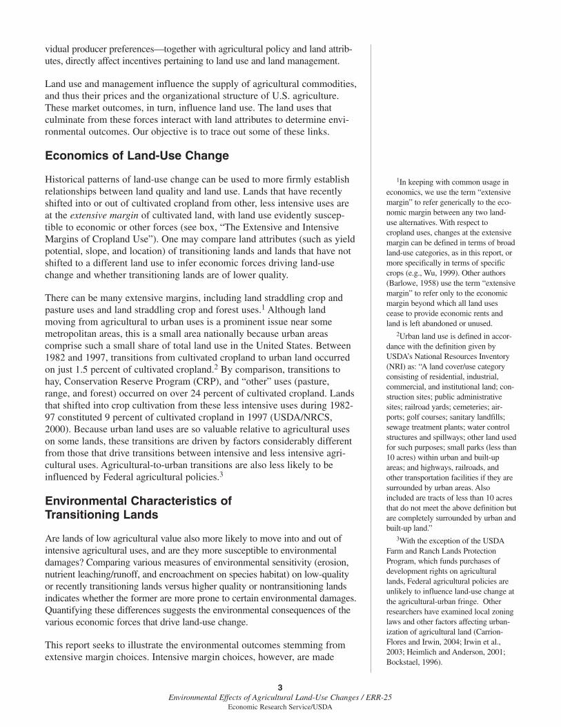
Regions that have more acreage of cultivated cropland also tend to haverelatively large movement of land both into and out of cultivated cropproduction. The Heartland, Northern Great Plains, and Prairie Gatewayaccount for about 70 percent of U.S. cultivated cropland, and have the mostland transitioning into and out of cultivated crop production (fig. 2.7). In allthree regions, CRP was a major factor in land transitioning out of cultivatedcropland (fig. 2.8).
Regions that started with a lot of cultivated cropland in 1982 also tended tohave large net reductions in cultivated cropland (fig. 2.7). The reduction incultivated cropland was particularly large in the Prairie Gateway (10.9million acres), where CRP enrollment was also high (9.6 million acres).Although the Southern Seaboard started with less cultivated croplandacreage, the net reduction from 1982 to 1997 was large, especially shifts tograzing and forests; 1.4 million acres, or 8 percent, of the cultivated crop-land in 1982 shifted to pasture and a similar amount shifted to forests by1997. In the Northern Crescent, the extensive margin of crop productionwas active in both directions, despite a relatively small base of cultivatedcropland and relatively little CRP enrollment.
10There were 5.3 million acres inuncultivated crops in both 1982 and1997 that moved to a less intensive usein 1987 or 1992 (with 4.6 million and0.5 million shifting to grazing andCRP). Some 1.8 million acres of landnot in uncultivated crops in either 1982or 1997 shifted to uncultivated crop-land from a less intensive use in 1987or 1992. In total, at least 7.1 millionacres changed use at the extensive mar-gin of uncultivated cropland, in addi-tion to the 16.5 million acres millionacres described earlier. The total move-ment of land at the extensive margin ofuncultivated crops thus exceeds 23.6million acres, more than half of the44.5 million acres of uncultivatedcrops in 1982.
11Environmental Effects of Agricultural Land-Use Changes / ERR-25
Economic Research Service/USDA

The fact that larger declines occurred in regions with more cultivated crop-land does not necessarily indicate that crop production is shifting towardregions with less initial cropland acreage. In fact, the four regions with thelargest cultivated cropland acreages (Heartland, Prairie Gateway, NorthernGreat Plains, and Northern Crescent) experienced the smallest percentagereductions in cultivated cropland area (fig. 2.9). On the other end of thescale, the Eastern Uplands region, which has the smallest acreage of culti-vated cropland, experienced the smallest net decline in absolute terms butthe largest decline in percentage terms. Reduction in cultivated croplandexceeded 20 percent in three regions: the Eastern Uplands, SouthernSeaboard, and Basin and Range. A region’s tendency to maintain cultivatedcropland (at the margin) likely reflects differences in soil quality, the scaleof production, government programs, and other factors affecting the relativeprofitability of growing crops.
So, the extensive margin of crop production is significantly larger than thenet change in land used for cultivated crops. Between 1982 and 1997, culti-vated cropland declined by 50 million acres, while more than 100 millionacres were shifted into or out of cultivated crops. These shifts (either grossor net) are not evenly distributed across regions, with absolute changeslarger in regions with the most cultivated cropland and percentage changesgreater in regions with relatively little cultivated cropland.
12Environmental Effects of Agricultural Land-Use Changes / ERR-25
Economic Research Service/USDA

13Environmental Effects of Agricultural Land-Use Changes / ERR-25
Economic Research Service/USDA

14Environmental Effects of Agricultural Land-Use Changes / ERR-25
Economic Research Service/USDA
15Environmental Effects of Agricultural Land-Use Changes / ERR-25
Economic Research Service/USDA
Figure 2.7
Shifts to and from cultivated cropland (all land uses), by region, 1982-97
Million acres
Source: 1997 National Resources Inventory.
Net changeShifts to cultivated croplandShifts away from cultivated cropland
Eastern Uplands
Basin and Range
Northern Crescent
Mississippi Portal
Fruitful Rim
Heartland
Northern Great Plains
Southern Seaboard
Prairie Gateway
-20 -15 -10 -5 0 5 10
Figure 2.8
Shifts from cultivated cropland to CRP and other agricultural and forest uses, by region, 1982-97
Million acres
Source: 1997 National Resources Inventory.
Shifts to CRPShifts to uncultivated cropland, grazing, forest, and other rural land
Eastern Uplands
Basin and Range
Northern Crescent
Mississippi Portal
Fruitful Rim
Heartland
Northern Great Plains
Southern Seaboard
Prairie Gateway
-15 -10 -5 0

Even if the amount of land used for crop production is relatively stable, thespecific land being used for crops is changing. So, have the economic andenvironmental characteristics of cultivated cropland been changing evenwhile cropland acreage remains constant? And is cultivated cropland at theextensive margin more or less vulnerable to environmental damage than theland that persists in cultivated crop production?
Finally, agricultural policy may affect the environmental characteristics ofcultivated cropland through its impact on the extensive margin of cropproduction. CRP enrollment is critical, given its role in shifting land fromcrop production in the three regions with most cultivated cropland. Howdoes CRP land compare environmentally with land converted to cultivatedcrops? Crop insurance may also have affected the extensive margin of cropproduction, but its effects are more difficult to quantify.
16Environmental Effects of Agricultural Land-Use Changes / ERR-25
Economic Research Service/USDA
Figure 2.9
Percentage shifts to and from cultivated cropland (all land uses), by region, 1982-97
Percent of cultivated cropland (1982)
Source: 1997 National Resources Inventory.
Net changeShifts to cultivated croplandShifts away from cultivated cropland
Heartland
Northern Crescent
Northern Great Plains
Prairie Gateway
Mississippi Portal
Fruitful Rim
Basin and Range
Southern Seaboard
Eastern Uplands
-50 -40 -30 -20 -10 0 10 20

Producers allocate land to the use they expect will yield the greatest benefitover time.1 In an agricultural context, maximizing benefits entails selectingwhich commodity to produce (e.g., corn, hay, or timber) and how, usingland as an input.2 The expected return to land depends on the price ofoutputs and (nonland) inputs, available technology (which can affect theper-unit cost of production), government policies, skills and preferences ofthe producer, and land quality.
Studies of land allocation, particularly among major land uses, have focusedon the role of land quality and policy in determining land use. Policy canaffect land-use decisions in a variety of ways. Price supports can alter therelative return between commodities that are supported and those that arenot (Wu and Segerson, 1995; Plantinga, 1996). The tax code may favorcertain land uses by its treatment of associated investments (Lichtenberg,1989). Crop insurance, by reducing the risk of crop production, maypromote crop cultivation where it is relatively risky (Goodwin et al., 2004;Wu, 1999). Government-funded infrastructure developments, such as floodcontrol projects, may also enhance the economic viability of crop produc-tion in particular areas (Stavins and Jaffe, 1990).
In these studies, the effect of market prices, technology, and policy are allconsidered in the context of the land’s ability to produce various goods andservices. While there is no single best indicator of land quality, soil produc-tivity—suitability of the soil as a medium for plant growth—is key for agri-cultural production. Most soil productivity definitions include attributes ofthe soil, climate, and topography. Existing studies have used a range ofindictors, including the Land Capability Classification (Plantinga, 1996;Hardie and Parks, 1997) and one or more specific soil parameters such aswater holding capacity (Lichtenberg, 1989; Wu, 1999; Wu and Brorsen,1995). As a rule, land quality attributes are fixed or change only slowly.Nonetheless, changes in markets, government policy, or technology mayfavor some types of land over others.
The characteristics of producers also affect land-use decisions. Producersmay assess returns to various land uses differently because of differences inmanagement skills, expectations about future prices or technology, risk aver-sion, or personal objectives. For example, lifelong crop farmers may bemore reluctant to shift from crop production to forestry than individualswho have some expertise in timber production. Likewise, producers whoseprimary occupation is not farming or forestry may allocate land to agricul-ture, forestry, or other uses based on preferences that are not centered onpotential return.
When a change in land use involves significant upfront costs (e.g., removingtrees to begin crop production) or delayed returns (e.g., converting land to
1In this report, we use the term“producer” to refer generically to theindividual making the land-use deci-sions for a parcel of land. This deci-sionmaker may or may not be theowner of the land. Land-use decisionsmay be made by the landowner, a landmanager or operator, or some combi-nation of the two. The ability of anoperator renting land to make land-usedecisions will depend on the terms ofthe cash or share lease contract and theability of the owner to monitor andenforce this agreement.
2Land may also be valued for awider range of goods, including recre-ational and ecological services.Producers can capture some (but notall) of these values by charging feesfor hunting or other recreational activi-ties. Producers may also value servicessuch as recreation, aesthetic beauty, orenvironmental protection even if theycannot be compensated monetarily forthem.
17Environmental Effects of Agricultural Land-Use Changes / ERR-25
Economic Research Service/USDA
Chapter 3
Land Quality and Land-Use Change

timber production), risk aversion, wealth, and discounting may be important.Producers who are particularly risk averse may be reluctant to make a large,upfront investment or wait many years to receive a return, even when thereturn is likely to be higher than that of other land uses. Even if they are notrisk averse, producers with limited assets may have difficulty financing along-term investment. Also, the more an individual discounts future returns,the less likely he or she is to undertake a long-term investment. For example,if crop production yields an average annual return (to land) of $40 per acre,the net present value (NPV) of returns discounted at 4 percent per year over20 years is $544. A pulpwood harvest occurring at 20 years would have to net$1,192 per acre to yield an equivalent NPV (1192*(1+.04)^20=544). If futurereturns are discounted at 6 percent, however, the timber harvest would have toyield a net of $1,471 per acre to rival crop production.
Over time, market transactions tend to direct land to the owners who valuethe land most and into the uses they perceive as most valuable. Consider thesale of land that is in grazing use but has some potential for profitable cropproduction. Some bidders may believe that grazing is the most valuable useof the land and submit bids accordingly. Others may focus on the land’scrop production potential and submit bids that reflect returns to cropproduction (less the cost of converting the land to crop production). If thehigh bid is from an individual who believes that the land is more valuable incrop production, it is likely that land-use conversion will quickly follow thesale. Because agricultural land markets in certain areas can be “thin” (withonly a small proportion of land sold in any given year), reallocation of landuse may take many years and be interrupted by changes in economic condi-tions that alter individuals’ views on relative returns.
A Model of Land Allocation and Land Quality
For the purpose of our conceptual model, we assume that land quality canbe defined by a single valued index that primarily measures soil produc-tivity. This index captures the potential of land to generate economic returnsfor the private owner or operator (distinct from an environmental qualityindex measuring benefits to society). Soil productivity refers to the suit-ability of the soil and climate as a plant growth medium (see box, “SoilQuality Indicators”).
Location may be an important determinant of land quality in several ways.The proximity of land to centers of population and employment is critical indetermining the potential value of land for development (Bockstael, 1996).Local amenities, such as open space and rural “character,” may also enhancethe value of land for residential development (Wu et al., 2004). In terms ofcommodity production, distance to markets may also be important. Forexample, local grain prices depend in part on shipping cost. For bulkiercommodities such as hay or timber, proximity to markets is even more crit-ical. Distance of land to population centers may also affect the profitabilityof providing recreational services. In some cases, the value of recreationalservices that can be captured by the producer may tip the balance in a land-use decision. For example, grassland may provide livestock grazing duringthe spring and summer, and be used for hunting in the fall and winter
18Environmental Effects of Agricultural Land-Use Changes / ERR-25
Economic Research Service/USDA

months. However, given the likelihood that nearby land could also providesimilar amenities, the recreational services must be valued by enough peoplefor them to be a viable land use.
Figure 3.1a shows the relationship between land quality and returns forthree hypothetical land uses given fixed prices, technology, and policy. Theconcave shape of the curves (decreasing upward slope as land qualityincreases) is based on the assumption that the genetic capacity of plants willincreasingly become the limiting factor in production as land quality rises.Land use A is best able to use land of very low quality, but also reaches itsfull potential at a relatively low level of land quality. Land use C, on the
19Environmental Effects of Agricultural Land-Use Changes / ERR-25
Economic Research Service/USDA
In allocating land among agricultural and forest uses, productivity in termsof crop, forage, or timber production is a key indicator of land quality.Productivity refers to the suitability of the soil as a plant growth mediumand the favorability of the climate. While productivity itself is complex,some useful proxies include crop yields or yield potential, one or morespecific soil attributes, such as soil water holding capacity (e.g., see Licht-enberg, 1989; Wu, 1999), and indices that combine multiple soil attributesinto a single number such as the Productivity Index (Pierce et al., 1983) orthe soil rating for plant growth (SRPG; Soil Survey Staff, 2000).
Topography can also affect productivity as the loss of soil and nutrientsthrough surface runoff can result in higher input costs and reduced soildepth, reducing soil productivity over time. Highly erodible land, which isoften steeply sloping, is less likely to be used for crop production (Mira-nowski and Hammes, 1984). In at least one index of soil productivity(SRPG), slope reduces the overall soil productivity score. Steeply slopingland can also be difficult to farm efficiently with large machinery typical ofmodern crop production.
SRPG is an index of inherent soil productivity based on soil’s physical,chemical, and biological factors as well as topography and climate. WhileSRPG is based largely on inherent properties of the soil such as texture andwater holding capacity, the productivity of specific tracts of land can bedamaged over time by soil erosion. SRPG was originally developed byNatural Resource Conservation Service soil scientists for use in imple-menting the Conservation Reserve Program (CRP).
While the SRPG rating and other soil productivity measures are indicatorsof economic potential, they are proxies. A more direct measure is potentialyield. Potential yields are estimated in a number of ways, including experi-mental plots, and are intended to reflect the management practices yieldingthe highest economic return. Estimated irrigated and non-irrigated yieldsfrom the Soil Conservation Service’s (now NRCS) Soils 5 data are linkedto the National Resources Inventory (NRI) data set. The Soil SurveyGeographic (SSURGO) data from NRCS are the most up-to-date source ofyield and soil productivity information, and are being digitized for theentire country.
Soil Quality Indicators

other hand, cannot use low-quality soils but is better able to take advantageof the greater plant growth potential on high-quality land.
If these curves reflect a market-level assessment of the relative value of thethree land uses, land with quality (Q) less than X will be idle (not devotedto any of the three uses considered in figure 3.1a); land with qualitybetween X and Y will be devoted to use A; land with quality between Y andZ will be devoted to use B; and land with quality greater than Z will bedevoted to use C. The producer is indifferent between land uses A and B atpoint Y, and is indifferent between uses B and C for land of quality Z.
20Environmental Effects of Agricultural Land-Use Changes / ERR-25
Economic Research Service/USDA
Figure 3.1a
Land quality and relative return to three hypothetical land uses
Land qualityX Y Z
A
B
C
Expected return(per acre)
Figure 3.1b
Land quality and relative return to three hypothetical land uses: Effect of decline in output price
Expected return(per acre) C
C’
Land qualityX Y Z Z’
A
B

These stylized predictions are supported by the data on the distribution of landquality across land uses. Figure 3.2 shows the distribution of land quality, asdefined by the soil rating for plant growth (SRPG), by land use, averaged over1982-97. The SRPG is a measure of soil productivity that can take values of 0-100. While there is land of different qualities devoted to every use, lands incultivated crops include a greater proportion of high-productivity land (SRPG67-100) and a smaller proportion of low-productivity land (SRPG 0-33) thanany other land-use category. These results imply that cultivated crops are bestable to take advantage of high-productivity land but are relatively unprofitableon low-quality land. Uncultivated cropland and CRP include more medium-quality land (SRPG 34-66) than other land-use categories. Finally, pasture,forest, and rangelands include more low-productivity land than the croplandcategories or CRP (which is former cropland). Forest and rangeland alsoinclude less high-quality land than other land-use categories.
Land enrolled in CRP is likely to be of lower quality than cultivated crop-land on average as a result of program-specific objectives and economicincentives for participating. First, USDA targets highly erodible land amongother environmental factors in the Environmental Benefits Index (EBI), theselection criteria used for selecting CRP parcels. We show later that highlyerodible land is also less productive on average, so the program indirectlytargets land with lower soil productivity.3 Second, the cost of enrolling landis another component of the selection criteria so that, given similar environ-mental characteristics, producers with less to lose from participating aremore likely to be accepted into CRP. Thus, lower value land is directlytargeted as well. USDA also sets soil-specific caps (based on SRPG) on themaximum annual rental payments allowed under the program. All else being
3The relationship between soil pro-ductivity and erodibility is examinedin detail in the next chapter.
21Environmental Effects of Agricultural Land-Use Changes / ERR-25
Economic Research Service/USDA
Figure 3.2
Distribution of different agricultural uses, by soil productivity index –Soil rating for plant growth
Cultivatedcrops
CRP Uncultivatedcrops
Pasture Forest Range0
10
20
30
40
50
60
70
PercentSRPG 0-33SRPG 34-66SRPG 67-100
Source: ERS analysis of 1997 NRI and Soil Survey Geographic data set.
Note: SRPG = soil rating for plant growth. Numbers depict the average share of land in each cell across each soil productivity category from 1982 to 1997, with shares in each cell summing to 100 percent. As seen by moving from left to right across each row, land in more intensive land uses, such as cultivated crops, generally has a higher proportion of high-productivity soils (SRPG 67-100) and a lower percentage of low-productivity soils (0-33) than land in less intensive uses, such as rangeland.

equal, for any particular soil type, producers with economic benefits fromcrop cultivation near (or above) the cap will have smaller incentives toparticipate in CRP than producers on lower quality land. Because we do notobserve all sources of variation in soil productivity, the relative productivityof lands enrolling in CRP may be even lower than our analysis suggests.
Change in market prices, technology, and policy can be depicted as shifts inone or more of the curves in figure 3.1a. If, for example, the price ofoutput(s) produced by land use C decreases, the curve for land use C wouldshift downward (see C’ in figure 3.1b).4 If returns to other land uses areunchanged, land with quality between Z and Z’ would shift from use C touse B. Similar shifts (in the opposite direction) may be observed with tech-nical changes that lower per-unit production costs.
Economic Characteristics of Transitioning Lands
The conceptual model suggests that low-quality cultivated croplands (rela-tive to other cultivated cropland) would be most likely to shift to unculti-vated cropland, CRP, and other agricultural and forest uses as marketconditions, government policies, or technology change. Similarly, theorysuggests that the relatively high quality land in uncultivated crops andpasture would be on the margin with cultivated cropland while relativelylow-quality uncultivated cropland would be on the margin with forest andrangeland. Following the same logic, the relatively high-quality lands inforest and range would be those most likely to transition to crop production.
This pattern is borne out by an examination of land quality for various cate-gories of land-use change over 1982-97. This is the longest period for whichthe NRI data are available and reveals the largest amount of cropland changes.Land that was in cultivated in 1982 and stayed in cultivated crop production(fig. 3.3, row 1, column 1) includes a higher proportion of high-productivityland and a lower proportion of low-productivity land than land that moved toanother use by 1997 (fig. 3.3, row 1, columns 2-4). Likewise, land moving tocultivated crop production from another use (row 2 and 3, column 1) includes ahigher proportion of high-productivity land and a lower proportion of low-productivity land than noncultivated lands that remained in or moved toanother noncultivated use (rows 2-3 and columns 2-4). In general, land thatstayed in or moved to cultivated cropland is more likely to have high-produc-tivity land than land in (or moving between) noncultivated land uses.5
While the SRPG rating is one indicator of economic potential, it is a proxy. Amore direct measure is the potential yield—the amount of a given crop that canbe produced per unit of land under the management practices providing thehighest economic return (see box, “Soil Quality Indicators”). Figure 3.4 showspotential yields, relative to crop reporting district (CRD) averages, for fourmajor crops (corn, soybeans, wheat, and alfalfa hay) in the cells of the land-usechange matrix associated with our four key land uses.6 The bar in each cellrepresents the average relative yield for each crop.
By focusing on yields relative to the average for a relatively small geographicarea, we compare yields while holding constant other factors that are common
22Environmental Effects of Agricultural Land-Use Changes / ERR-25
Economic Research Service/USDA
4Curve shifts need not be parallel.If lower land quality has less output(e.g., a lower corn yield), then achange in the output price would havea larger per-acre effect on higher qual-ity land. Technology change may notaffect all types of land equally, either.Lichtenberg (1989) showed that soilswith greater water holding capacity inthe Nebraska sand hills were morelikely to be shifted from small grainsand hay to row crops with the develop-ment of center-pivot irrigation. 5Lands observed in cultivation in both1982 and 1997 include some lands thatshifted out of cultivation and thenshifted back over the course of thisperiod. Excluding these lands from ourcategory of lands remaining in cropcultivation would likely strengthen ourfindings regarding the relative soil pro-ductivity at the extensive margin ofcultivated cropland.
6Most States have between six andnine CRDs, multicounty units used byUSDA in gathering data. Each NationalResources Inventory (NRI) point isassigned relative yields, which are theratio of the point-specific yield to theaverage yields, for all four land uses inthe CRD. Estimated yields are from theSoil Conservation Service’s (nowNRCS) Soils 5 data. While yields datafrom the Soil Survey Geographic(SSURGO) have been most recentlyupdated, we used Soils 5 data for thisanalysis as our focus is on relative(rather than absolute) yield levels, andSoils 5 data had a wider geographiccoverage as of the time of our study.
Soils 5 yields are also not available forall soils; the less likely land is to beused for crop production, the less likelyit is to be assigned a yield in the Soils 5data series. Because potential cropyields on this land are likely to be rela-tively low, the exclusion of these landsis likely to bias estimates for averagerelative yield upward for land in lessintensive uses. Thus, differences in rela-tive potential yields may be even morepronounced than indicated in figure 3.4.

to this region. Given that prices for agricultural output and inputs are not likelyto vary much within a CRD, estimated differences in yields are strong indica-tors of differences in the profitability of different subsets of land.
Using relative potential yields gives roughly the same pattern of land useand land quality as SRPG, though it provides some additional insights. Ingeneral, land in cultivated crops has higher yield potential than land in otheruses (fig. 3.4, compare column 1 to columns 2-4). Average yields for land
23Environmental Effects of Agricultural Land-Use Changes / ERR-25
Economic Research Service/USDA
Figure 3.3
Land-use change and land quality – Soil rating for plant growth
Percent
SRPG 0-33SRPG 34-66SRPG 67-100
Source: ERS analysis of 1997 NRI and Soil Survey Geographic (SSURGO) data set.
Cultivated in1997
Uncultivated in1997
CPR in 1997 Grazing, forest,other in 1997
0
20
40
60
80
39
54
7
26
57
16 20
65
1527
56
17
Cultivated in1997
Uncultivated in1997
CPR in 1997 Grazing, forest,other in 1997
0
20
40
60
80
26
58
16 16
59
2514
69
18 18
53
29
Cultivated in1997
Uncultivated in1997
CPR in 1997 Grazing, forest,other in 1997
0
20
40
60
80
26
57
18 20
53
2718
58
24
7
35
58
Cultivated cropland in 1982
Uncultivated cropland in 1982
Grazing, forest, and other in 1982
Notes: Numbers depict the share of land in each cell across each soil productivity category, with shares in each cell summing to 100 percent. As seen by moving from left to right across each row, land that transitioned to (or remained) in a more intensive land use, such as cultivated cropland, generally has a higher proportion of high-productivity soils (SRPG 67-100) and a lower percentage of low-productivity soils (0-33) than land transitioning (or remaining) in a less intensive use, such as grazing, forest, and other land. As seen by moving from top to bottom along each column, land in more intensive land uses generally has a higher proportion of high-productivity soils (SRPG 67-100) and a lower percentage of low-productivity soils (0-33) than land in less intensive uses.

that was in cultivated cropland in both 1982 and 1997 are generally higherthan for land that moved from cultivated cropland to another use. Theexception is alfalfa, where potential yields are higher on uncultivated crop-land (row 1, column 2). Also, potential yields of corn, soybeans, and wheaton land that moved to uncultivated crops (row 1, column 2) are almost ashigh as for land that remained in cultivated cropland. Moreover, land thatshifted from cultivated crops to CRP (row 1, column 3) had lower yieldsthan all other land moving from cultivated crops (row 1, column 4).
Clear economic differences exist across lands at the extensive margin ofcrop production. Most strikingly, land enrolled in CRP appears to be the
24Environmental Effects of Agricultural Land-Use Changes / ERR-25
Economic Research Service/USDA
Figure 3.4
Land-use change and land quality – Expected crop yields
Percent difference from CRD average
Alfalfa hayWheatSoybeansCorn
Source: ERS analysis of 1997 NRI and Soils 5 data.
Cultivated cropland in 1982
Uncultivated cropland in 1982
Grazing, forest, and other in 1982
Cultivated in1997
Uncultivated in1997
CRP in 1997 Grazing, forest,other in 1997
-10
-5
0
5
10 75 6
4 4 5 57
2 1 0
-3
3 3 3 3
Cultivated in1997
Uncultivated in1997
CRP in 1997 Grazing, forest,other in 1997
-10
-5
0
5
104 5 5
8
2 2 2
7
-8-1
0
-8
0
-1
0
4
Cultivated in1997
Uncultivated in1997
CRP in 1997 Grazing, forest,other in 1997
-10
-5
0
5
10
2 3 3
-1
0 02
5
1 0
-3-10
-3 -3 -4 -3
Note: To account for variations in climate and other nonland quality factors that could cause yields to vary spatially, each NRI point is assigned relative yields that are the ratio of the point-specific yield to the average yields, for all four land uses, in the crop reporting district (CRD). For each cell, the average relative yields are reported.

lowest quality land in a crop reporting district across each of the croplandcategories considered. Cultivated cropland enrolled in CRP is just slightlyabove average for corn, soybeans, and wheat and below average for hay. Itappears to be less productive than land converting to other agricultural andforest uses. Uncultivated cropland enrolled in CRP follows the same pattern.
Many of the yield differences observed are small. Estimated yields on landin cultivated crops in both 1982 and 1997 are 4-7 percent above CRD aver-ages (fig. 3.4, row 1, column 1), while land that was in grazing, forest, orother uses in both years had yields 3-4 percent below CRD averages (row 3,column 4). The overall pattern is striking given the coarseness of the under-lying data. The Soils 5 data do not reflect all of the factors affecting yieldson each land parcel. The data are specific to a soil map unit and captureonly general variation in potential yields based on soil type. Consideringadditional parcel-level characteristics would tend to increase the variation inestimated yields within a small geographic area, and thus magnify thedeparture in yields from the CRD average.
Conclusion: Land At The Extensive MarginTends To Be of Lower Quality
The theoretical model of land allocation provides a framework for analyzingdata on the economic characteristics of lands at different extensive margins.Two land quality indicators—SRPG and potential crop yields—suggest clearpatterns in the relative profitability of lands at different extensive margins, withhigher (lower) quality lands more likely to be devoted to more (less) intensiveland uses. The extensive margin of cultivated cropland is largely cultivatedcropland that is of lower quality than other cultivated cropland and land in lessintensive uses is higher quality than other land in those uses. These results indi-cate that land quality is, indeed, a critical factor in the allocation of land amongagricultural and forestry uses. Lands enrolled in the CRP appear to be ofparticularly low quality relative to other land in the same geographic area.
The indicators examined do not fully explain land use. For example, someland with high productivity (SRPG 67-100) is in other agricultural andforest uses, while some land in cultivated crops has low productivity (SRPG0-33). Of course, soil productivity indicators do not capture every dimensionof land quality that is important to agricultural land-use decisions. An unfa-vorable location far from infrastructure and transportation facilities, forexample, may make land otherwise quite suitable for crop productionunprofitable for this purpose.
In this chapter, land quality was defined narrowly to focus on land charac-teristics that are of direct economic value in agricultural production.However, the environmental impact of land-use change at the extensivemargin of cultivated cropland will depend largely on factors like erodibilityand nutrient runoff potential. Some analysts have assumed that land whichis economically marginal for crop production is also more environmentallysensitive than other cropland. In the next chapter, we test this assumption byexamining the relationship between economically marginal croplands anddifferent indicators of environmental sensitivity.
25Environmental Effects of Agricultural Land-Use Changes / ERR-25
Economic Research Service/USDA
Agricultural production, particularly cultivated crop production, can affectthe environment in many ways. But is the extensive margin of cultivatedcrop production more susceptible to soil erosion or nutrient loss thanaverage cropland? These agri-environmental problems have been a majorfocus of U.S. agri-environmental policy over the past two decades. We alsoexamine whether changes in cultivated cropland could be affecting habitatthat is important to imperiled species of birds and other wildlife. Imperiledspecies are those classified by NatureServe as either “critically imperiled”or “imperiled” at the national level, receiving a Global Conservation Status(G) rank of 1 or 2, respectively. These data are the most comprehensivemeasure of U.S. biodiversity conservation status (see Appendix C).
We analyze the relationship between soil productivity, environmental sensi-tivity, and land use at both the local and national levels. At the local level, wecompare differences from averages by Crop Reporting District (CRD). MostStates have between six and nine CRDs, which are multicounty areas used byUSDA for data gathering purposes. When environmental sensitivity varieswidely at that local level, focusing on small geographic areas ensures that localdifferences are not averaged out, as they could be in national averages. We lookat differences from national averages to capture broader inter-regional differ-ences. For example, wind erosion occurs mostly on semi-arid regions of theNorthern and Southern Plains. But at a local level, land may be quite similar interms of erodibility. Finally, available data are not always sufficient to capturelocal variations in environmental sensitivity. In these cases, comparisonsagainst national averages are necessary, even if local variation is significant.
Lands With Low Soil Productivity are MoreVulnerable to Erosion Damage
We measure the soil’s sensitivity in terms of erosion using the erodibilityindex (EI) and the estimated average annual rate of soil erosion. The EI isdefined by the ratio of inherent erodibility to the soil loss tolerance.Inherent erodibility for a given soil is the rate of erosion (tons per acre peryear) that would occur on land that was continuously clean tilled throughoutthe year.1 The soil loss tolerance is the rate of soil erosion that can occurwithout significant long-term productivity loss. Thus, while the erodibilityindex is independent of land use and management, it measures the fragilityof the soil in terms of erosion, capturing both the potential of a soil to erodeand its resistance to erosion damage.
Actual levels of soil erosion depend greatly on land use and management,making comparisons across different land uses difficult. On land in culti-
1Wischmeier and Smith (1978) andSkidmore and Woodruff (1968) providedetailed descriptions of the estimationof inherent erodibility for rainfall ero-sion and wind erosion, respectively.
26Environmental Effects of Agricultural Land-Use Changes / ERR-25
Economic Research Service/USDA
Chapter 4
Environmental Characteristicsof Economically Marginal
Cropland

vated crop production, soils are frequently exposed to the erosive forces ofrainfall and wind, and tend to erode more quickly than land in continuousgrass or tree cover. However, meaningful comparisons can be made acrosslands of different soil productivity levels that are, nonetheless, devoted tothe same land use. Average annual rates of erosion are estimated (for NRIdata points) using the Universal Soil Loss Equation (USLE; Wischmeier andSmith, 1978) and the Wind Erosion Equation (WEE; Skidmore andWoodruff, 1968).
At the local (CRD) level, lands with lower soil productivity do tend to bemore inherently erodible for wind and, especially, rainfall (fig. 4.1, top row).Low-productivity land (SRPG 0-33) is, on average, 40 percent more suscep-tible to rainfall erosion than the CRD average, while high-productivity land(SRPG 67-100) is 25 percent less erodible. The critical factor behind thesedifferences is the steepness of slopes. On steeply sloping land, water runsoff quickly, often carrying soil with it. Topography can also affect soilproductivity as the loss of soil and nutrients through surface runoff canresult in higher input costs and reduced soil depth. In the SRPG index, slopereduces the overall soil productivity score.
For wind erosion, low-productivity land is, on average, 34 percent moreerodible than the CRD average, while high-productivity land is 18 percentless erodible. At a local level, differences in wind erodibility derive fromdifferences in climate (prevailing winds) and the susceptibility of the soil towind erosion. At a national level, differences in wind erosion are primarilydue to regional differences in climate; land in more arid regions is morelikely to be eroded by wind.
At a national level, the relationship between soil productivity and erodibilityis similar to that observed at the local level, but more pronounced for bothrainfall and wind erosion (fig. 4.1, second row). For example, wind erodi-bility ranges from 62 percent above the national average for lands with lowproductivity to 47 percent below the national average for lands with highsoil productivity.
Potential crop yields also tend to be lower on highly erodible cropland(HEL).2 Average potential crop yields for HEL range from 77 percent (foroats) to 82 percent (for hay) of non-HEL yields (table 4.1).3 This suggeststhat, on average, HEL is about 20 percent less productive, relative to non-HEL in the same CRD. Still, the productivity of HEL varies considerably. Insome CRDs, potential yields on HEL are substantially above—close todouble for alfalfa hay—those for non-HEL (maximum yield ratio, table4.1). In other CRDs, potential yields on HEL are a third or less of those onnon-HEL (minimum yield ratio, table 4.1). Despite this variation, at thenational level, the highest potential yields always occur on non-HEL for thecrops examined.
Soil Productivity And Nutrient Losses
Nutrient runoff depends on both the inherent characteristics of land(including climate) and the way it is used and managed. Lands in cropproduction tend to have higher rates of nutrient loss because they receive
2Highly erodible land (HEL) has anerodibility index (EI) of 8 or more.
3Using a Geographic InformationSystem (GIS), estimated yields andHEL designations are overlaid withCRD boundaries to estimate the ratioof yields on HEL and non-HEL landwithin each CRD. Estimated yields arefrom Soil Survey Geographic(SSURGO) data, the most up-to-datesource of yield and soils informationavailable. We are limited to cropreporting districts that have yield esti-mates for both HEL and non-HEL, butwe have over 200 observations foreach of these crops: alfalfa hay, corn,oats, soybeans, and wheat.
27Environmental Effects of Agricultural Land-Use Changes / ERR-25
Economic Research Service/USDA

more fertilizer and, because of tillage, are more susceptible to nutrient trans-port from rainfall runoff and soil erosion. No indicator of inherent suscepti-bility to nutrient loss exists. But meaningful comparisons can be madeamong lands that are in the same use but vary in soil productivity.
Potential nitrogen and phosphorus loss to water are simulated using theEnvironmental Policy Integrated Climate Model (EPIC) and matched withland-use and soil information from the NRI and SSURGO data sets, respec-tively. EPIC is a crop biophysical simulation model that is used to estimatethe impact of management practices on pollution discharged at the fieldlevel (Mitchell et al., 1998). It uses information on soils, weather, land use,and land management practices—including fertilizer rates—and producesestimates of resulting erosion and nutrient loss to the environment (as wellas other indicators). Land use and management practices used in the EPIC
28Environmental Effects of Agricultural Land-Use Changes / ERR-25
Economic Research Service/USDA
Figure 4.1
Erodibility index relative to local and national averages, by land quality classification
Percent difference from US average
Percent difference from CRD average
Wind erodibility indexRainfall erodibility index
Source: ERS analysis of 1997 National Resources Inventory and Soil Survey Geographic data.
Soil rating forplant growth,
0-33
Soil rating forplant growth,
34-66
Soil rating forplant growth,
67-100
-100
-50
0
50
100
40 345 1
-25 -18
Soil rating forplant growth,
0-33
Soil rating forplant growth,
34-66
Soil rating forplant growth,
67-100
-100
-50
0
50
100 67 62
-3
12
-24-47
Notes: Point-level data are compared with the average for each Crop Reporting District (CRD) and for all agricultural and forest land in the United States. A CRD is a multicounty area defined for data gathering purposes by USDA’s National Agricultural Statistics Service (NASS). The soil rating for plant growth is an index of soil productivity based on many biological, chemical, and physical soil properties as well as topography and climate. In 1997, land with SRPG estimates of 0-33, 34-66, and 67-100 comprised 38, 44, and 18 percent of the private agricultural and forest land in the contiguous 48 States.

management files are based on existing land use, cropping patterns, andmanagement practices for highly erodible (HEL) and non-highly erodible(NHEL) land in 45 farm production regions (see appendix B for details).
At the local (CRD) level, the potential for nutrient loss to water increases asland quality (SRPG) declines (fig. 4.2, top row). For low-productivity land(SRPG 0-33), potential nutrient losses exceed CRD averages by 3 to 7percent for all four nutrient loss categories (nitrogen loss to surface water,nitrogen loss to estuaries, nitrogen leaching to groundwater, and phosphorusloss to surface water). On high-productivity land (SRPG 67-100), losses are7 to 12 percent less than CRD averages for all categories. Potential nutrientloss is very close to CRD averages on medium-productivity land (SRPG 34-66). However, these results are based on environmental modeling in whichlocal variation is limited. Within CRDs, differences in nutrient loss aredriven by differences in soil erodibility. Higher erodibility is often associ-ated with lower soil productivity and greater nutrient transport with soil.Also, the available data do not generally capture variations in nutrient appli-cations and cropping patterns within local areas.
At the national level (fig. 4.2, bottom row), differences in nutrient lossacross productivity classes are not as uniform as at the local level.Nitrogen loss to surface water is highest (6 percent above average) onlow-productivity land but lowest (6 percent below average) on medium-quality land. Nitrogen leaching to groundwater is highest on medium-quality land (14 percent above average), but 9 and 13 percent belowaverage on the other land classes. Nitrogen surface runoff and nitrogenleaching appear to have an inverse relationship: when surface runoff ishigh, leaching is low and vice versa. Nitrogen runoff to estuaries variesonly slightly since this is as much a function of location as soil character-istics. Finally, phosphorus runoff is lowest for lands with medium soilproductivity (5 percent below average) and highest for lands with high soilproductivity (7 percent above average).
The pattern of nutrient loss across land quality classes may be theproduct of offsetting trends in inherent susceptibility to nutrient loss andnutrient application. As soil productivity declines, erodibility and landslope tend to increase, potentially increasing the proportion of applied
29Environmental Effects of Agricultural Land-Use Changes / ERR-25
Economic Research Service/USDA
Table 4.1
Comparison of average crop yields on HEL and non-HEL, by soil survey unit
Average non-irrigated yield Ratio of HEL to Non-HEL yields1
Crop Highly erodible Standard No. ofAll land land (HEL) Average Median deviation Min. Max. observations
Alfalfa hay 3.7 2.7 0.82 0.79 0.22 0.27 1.95 215Corn 89.2 67.5 0.78 0.76 0.19 0.28 1.62 320Oats 65.3 47.4 0.77 0.76 0.22 0.33 1.70 222Soybeans 36.0 28.2 0.78 0.76 0.17 0.33 1.32 219Wheat 31.5 22.3 0.78 0.78 0.21 0.33 1.73 2011 Ratios are for non-irrigated yields within a soil survey unit, a geographic area cutting across counties. Average values are weighted by theamount of cropland within each soil survey unit. Highly erodible land (HEL) is land with an erodibility index (for either rainfall or wind erosion) of eight or more.
Source: ERS analysis of Soil Survey Geographic (SSURGO) Data set. SSURGO is the most detailed level of soil mapping conducted by USDA’s Natural Resources Conservation Service.

nutrients that are lost to the environment. Because the crop yield potentialis generally lower for less productive lands, these lands may receive morefertilizers than higher quality lands so as to compensate for the lowerproductive capacity of the soil. Alternatively, the relative benefits andcosts of fertilizer applications could imply that these lands receive lessfertilizer than higher quality lands, reducing the size of the overall poolof nutrients from which runoff can occur. On the other hand, even if thenutrient pool is smaller, lower crop yields also imply that the crop usesfewer nutrients, perhaps leaving just as much “excess” nutrient, which issusceptible to runoff and leaching.
30Environmental Effects of Agricultural Land-Use Changes / ERR-25
Economic Research Service/USDA
Figure 4.2
Nutrient runoff potential for cultivated cropland relative to local and national averages, by land quality classification
Percent difference from US average
Percent difference from CRD average
P to Surface WaterN LeachingN to EstuaryN to Surface Water
Source: ERS analysis of 1997 National Resources Inventory, Soil Survey Geographic data, and nitrogen (N) and phosphorus (P) indicators based on the Environmental Policy Integrated Climate model.
Notes: Point-level data are compared twith the average for each Crop Reporting District (CRD) and for all agricultural, forest, or other rural land in the contiguous United States. A CRD is a multicounty area defined for data gathering purposes by USDA’s National Agricultural Statistics Service (NASS). The Soil Rating for Plant Growth (SRPG) is an index of soil productivity based on many biological, chemical, and physical soil properties as well as topography and climate. In 1997, land with SRPG estimates of 0-33, 34-66, and 67-100 comprised 38, 44 , and 18 percent of the private agricultural and forest land in the contiguous 48 States.
Soil rating forplant growth,
0-33
Soil rating forplant growth,
34-66
Soil rating forplant growth,
67-100
-20
-10
0
10
20
47
3 50
-1
0 0
-7-12
-7 -9
Soil rating forplant growth,
0-33
Soil rating forplant growth,
34-66
Soil rating forplant growth,
67-100
-20
-10
0
10
20
6
-1
-9
2
-6
0
14
-5
2 2
-13
7

Our analysis until now has uncovered three relationships:
� Less productive croplands are those most likely to lie on the extensivemargin
� Lands that are less productive for crop production also tend to be moreenvironmentally sensitive in terms of potential erosion damage.
� Less productive lands are often more environmentally sensitive in termsof potential nutrient loss locally and sometimes nationally (although theevidence is not as strong as for erodibility).
Cropland That Converted to Other UsesWas More Prone to Erosion Damage andNutrient Loss
Rainfall Erosion. Lands that transitioned between cultivated crops and a lessintensive land use tend to have a greater potential for erosion damage thanland that was cultivated in both 1982 and 1997.4 At the local level, wherevariation in rainfall erosion can be large, land that was cultivated in 1982and 1997 had, on average, a rainfall erodibility index (EI) that was 20percent lower than the CRD average. Land that shifted to less intensiveuses, particularly to CRP, was generally more prone to erosion damage thanthe CRD average (fig. 4.3). High erodibility on CRP land is not surprising;erodibility is an important factor in CRP eligibility criteria and selection.Similar patterns are observed for land that started out as uncultivated crop-land and grazing/forest/other land (fig. 4.3). Similar relationships betweenrainfall erodibility and land use also emerge on a national scale (fig. 4.4).
Comparisons of estimated erosion rates (rather than the erodibiliy index)across different extensive margin lands can also be made by looking aterosion rates for the year when the land entering/leaving cultivated crops wasin cultivation.5 Land that moved from cultivated crops to another, less inten-sive use between 1982 and 1997 had relatively high 1982 erosion rates whencompared with land that stayed in crop production over that period (table 4.2).Land in cultivated crops in both 1982 and 1997 had an average rainfallerosion rate of 4.04 tons/acre/year (TAY), while land moving to uncultivatedcrops, CRP, or grazing/forest/other uses had erosion rates of 5.08, 5.97, and6.18 TAY. Land that moved to cultivated crop production from less intensiveuses had 1997 rates of rainfall erosion that were roughly equal to or higherthan for land that was cultivated in both 1982 and 1997 (table 4.2). Land culti-vated in both years had a 1997 average erosion rate of 3.06 TAY while the1997 rates on land that moved from uncultivated crops and from grazing,forest, and other uses were 2.99 TAY and 4.34 TAY, respectfully.
Wind Erosion. For wind-erodible soils, the erodibility index is also higher forland at the extensive margin of cultivated crop production than for land in culti-vated crops in both 1982 and 1997. At the local level, however, differences aremuch smaller than differences for rainfall erodibility (fig. 4.3). Land that wascultivated in 1982 and 1997 was less prone to damage from wind erosion (EI 2percent below the CRD average) than was transitioning land (EI 4-12 percentabove average). Land that moved to cultivated crop production from anotheruse also had higher potential for wind erosion damage than land cultivated in
4As noted previously, we comparelands transitioning and remaining incultivation over the 1982-97 period soas to obtain the maximum number ofobservations of lands transitioning atsome point over that period.Comparing lands changing overshorter 5-year periods would capturesome lands that shifted out of cultiva-tion and then returned to crop produc-tion from 1982 to 1997, but wouldreduce the overall observations of tran-sitioning lands. Because our group oflands that remained in the same usfrom 1982 to 1997 includes somelands that transitioned but thenreverted back to the starting use, theactual differences in the characteristicsof transitioning and not-transitioninglands are likely to be somewhat greaterthan our estimates imply.
5As land use changes, particularlybetween cultivated cropland and otherless intensive uses, erosion rates changedramatically. Thus, erosion rate changedue to land-use change does little toindicate the erodibility of extensive mar-gin land relative to other cultivatedcropland. Moreover, soil erosion gener-ally declined between 1982 and 1997(see table 4 in Claassen et al., 2004),further reducing the usefulness of“before” and “after” comparisons.
31Environmental Effects of Agricultural Land-Use Changes / ERR-25
Economic Research Service/USDA

both 1982 and 1997 (fig. 4.3). At the national level, results for wind erodibilityare mixed. The wind erodibility index on land that was cropped in 1982 and1997 (EI 11 percent above national average) is lower than on land that movedfrom cultivation to CRP (EI 139 percent above national average). On the otherhand, land that moved from cultivated crops to uncultivated crops (EI 4 percentabove national average) and to grazing, forest, and other uses (EI 17 percentbelow national average) had a lower erodibility rating (fig.4.4).
Estimated wind erosion rates also yield mixed results regarding the environ-mental sensitivity of land at the extensive margin of cultivated crop produc-tion. The average 1982 wind erosion rates on land converted from cultivated
32Environmental Effects of Agricultural Land-Use Changes / ERR-25
Economic Research Service/USDA
Figure 4.3
Erodibility index relative to local averages, by land use and land-use change category
Percent difference from CRD average
Source: ERS analysis of 1997 National Resources Inventory data.
Cultivated cropland in 1982
Uncultivated cropland in 1982
Grazing, forest, and other in 1982
Note: Data for each NRI point are compared with the average for each Crop Reporting District (CRD). A CRD is a multi-county area defined for data gathering purposes by USDA’s National Agricultural Statistics Service.
Wind erodibility indexRainfall erodibility index
Cultivated in1997
Uncultivated in1997
CRP in 1997 Grazing, forest,other in 1997
-100
-50
0
50
100
-20-2 -5
429
12 11 7
Cultivated in1997
Uncultivated in1997
CRP in 1997 Grazing, forest,other in 1997
-100
-50
0
50
100
-6
6 2
-1
61
11 16
-6
Cultivated in1997
Uncultivated in1997
CRP in 1997 Grazing, forest,other in 1997
-100
-50
0
50
100
14 525
6
94
21 34
-4
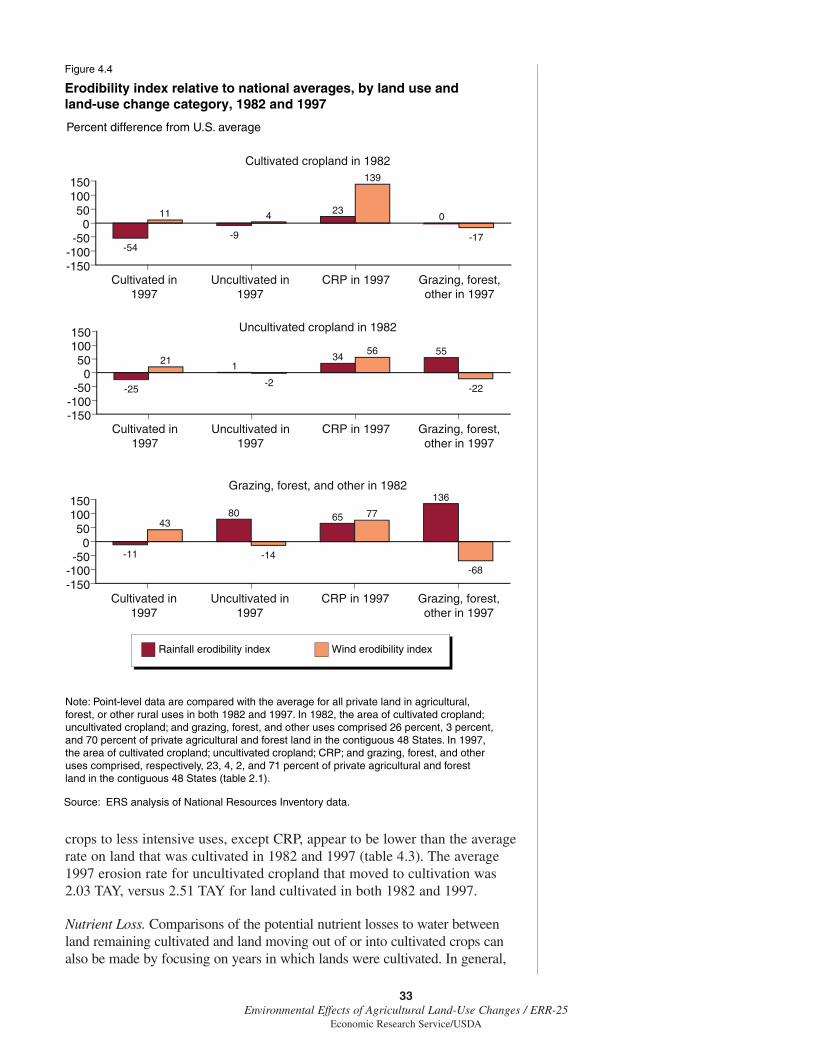
crops to less intensive uses, except CRP, appear to be lower than the averagerate on land that was cultivated in 1982 and 1997 (table 4.3). The average1997 erosion rate for uncultivated cropland that moved to cultivation was2.03 TAY, versus 2.51 TAY for land cultivated in both 1982 and 1997.
Nutrient Loss. Comparisons of the potential nutrient losses to water betweenland remaining cultivated and land moving out of or into cultivated crops canalso be made by focusing on years in which lands were cultivated. In general,
33Environmental Effects of Agricultural Land-Use Changes / ERR-25
Economic Research Service/USDA
Figure 4.4
Erodibility index relative to national averages, by land use and land-use change category, 1982 and 1997
Percent difference from U.S. average
Source: ERS analysis of National Resources Inventory data.
Cultivated cropland in 1982
Uncultivated cropland in 1982
Grazing, forest, and other in 1982
Note: Point-level data are compared with the average for all private land in agricultural, forest, or other rural uses in both 1982 and 1997. In 1982, the area of cultivated cropland; uncultivated cropland; and grazing, forest, and other uses comprised 26 percent, 3 percent, and 70 percent of private agricultural and forest land in the contiguous 48 States. In 1997, the area of cultivated cropland; uncultivated cropland; CRP; and grazing, forest, and other uses comprised, respectively, 23, 4, 2, and 71 percent of private agricultural and forest land in the contiguous 48 States (table 2.1).
Wind erodibility indexRainfall erodibility index
Cultivated in1997
Uncultivated in1997
CRP in 1997 Grazing, forest,other in 1997
-150-100-50
050
100150
-54
11
-9
4 23
139
0
-17
Cultivated in1997
Uncultivated in1997
CRP in 1997 Grazing, forest,other in 1997
-150-100-50
050
100150
-25
21 1
-2
3456 55
-22
Cultivated in1997
Uncultivated in1997
CRP in 1997 Grazing, forest,other in 1997
-150-100-50
050
100150
-11
4380
-14
65 77
136
-68

land moving between cultivated crops and a less intensive use had higherpotential for nutrient loss (when cultivated) than land that persisted in cultiva-tion in both 1982 and 1997.
Differences are largest for land that moved from cultivation in 1982 to unculti-vated crop production or grazing, forest, and other use in 1997 (fig. 4.5).6 Forexample, nitrogen runoff to surface water is 214 percent above the nationalaverage for land cultivated in 1982 and 1997, but 323 percent above averagefor land moving to uncultivated crops and 406 percent above average for landmoving to grazing, forest, and other uses. Cultivated lands have potentialnutrient losses far above the national average as uncultivated lands (themajority of the land base) receive minimal nutrient applications. CRP landappears to be less susceptible to nutrient loss than other lands moving out ofcultivation, possibly because the program tends to attract lands with low soilproductivity, where nutrient application rates may be lower. Moreover, CRP
6Because of data limitations, com-parisons are made only to nationalaverages.
34Environmental Effects of Agricultural Land-Use Changes / ERR-25
Economic Research Service/USDA
Table 4.2
Rainfall erosion, by land use and land-use change category (tons/acre/year), 1982 and 1997
1997 land use
1982 land use Cultivated Uncultivated Converation Reserve Grazing, forests, and cropland cropland Program other rural land
Uncultivatedcropland
Cultivatedcropland
Grazing, forests, andother rural land
5.08
0.60
0.343
0.403
0.103
6.185.97
4.34
2.99
0.333
0.75
3.062
0.6230.663
0.861.37
0.133
4.041
0.36
0.50
0.46
0.77
0.52
0.81
11982 erosion rates are in the upper left corner of each cell. Erosion rates for rainfall (sheet and rill erosion) are computed using the Universal Soil Loss Equation (USLE).2 1997 erosion rates are in the lower right corner of each cell.3 Erosion rate is for pasture only. NRI does not report erosion rates for rangeland, forest, and other rural land.
Source: ERS analysis of National Resources Inventory (NRI) data.
Table 4.3
Wind erosion, by land use and land-use change category (tons/acre/year), 1982 and 1997
1997 land use
1982 land use Cultivated Uncultivated Converation Reserve Grazing, forests, and cropland vropland Program other rural land
Uncultivatedcropland
Cultivatedcropland
Grazing, forests, andother rural land
2.21
0.33
0.073
0.103
0.013
2.337.57
2.85
2.03
0.083
0.48
2.512
0.1530.093
0.210.68
0.013
3.451
0.33
0.03
0.14
0.25
0.16
0.15
11982 erosion rates are in the upper left corner of each cell. Erosion rates for wind are computed using the Wind Erosion Equation (WEQ).2 1997 erosion rates are in the lower right corner of each cell.3 Erosion rate is for pasture only. NRI does not report erosion rates for rangeland, forest, and other rural land.
Source: ERS analysis of National Resources Inventory (NRI) data.

land is drawn heavily from arid regions where factors driving nutrient loss—rainfall runoff and rainfall-based soil erosion—are less intense.
Land shifting to cultivated crops from another use also appears to be moresusceptible to nutrient loss than land cultivated in 1982 and 1997 (fig. 4.6).For example, estimated potential nitrogen runoff on land converted fromuncultivated crops was 288 percent above the national average, versus 239percent for lands in cultivation in both 1982 and 1997.
35Environmental Effects of Agricultural Land-Use Changes / ERR-25
Economic Research Service/USDA
Figure 4.5
Potential (1982) nutrient runoff levels, by land use and land-use change categories
Percent difference from U.S. average
P to Surface WaterN LeachingN to EstuaryN to Surface Water
Source: ERS analysis of National Resources Inventory data and nitrogen (N) and phosphorus (P) indicators based on the Environmental Policy Integrated Climate model.
Notes: Point-level data are compared with the average for all private land in agricultural, forest, or other rural uses in both 1982 and 1997. Because grazing, forest, and other uses is the largest land-use category, lands in cultivated and uncultivated cropland in 1982 are generally significantly above average in terms of potential nutrient runoff levels. In 1982, the area of cultivated cropland; uncultivated cropland; and grazing, forest, and other uses comprised 26, 3, and 70 percent of the private agricultural, forest, and other rural land in the contiguous 48 States (table 2.1).
Cultivated in1997
Uncultivated in1997
CRP in 1997 Grazing, forest,other in 1997
-150
0
150
300
450
214 19495
28
323 354
193
66164
10948 17
406 417315
124
Cultivated in1997
Uncultivated in1997
CRP in 1997 Grazing, forest,other in 1997
-150
0
150
300
450
89 10638
-14
126187
48 1479 47
-5 -23
174 19693 61
Cultivated in1997
Uncultivated in1997
CRP in 1997 Grazing, forest,other in 1997
-150
0
150
300
450
-34 -28 -59
22
-15
2
-55
50
-36 -48 -69
14
-59 -40 -13 -7
Cultivated cropland in 1982
Uncultivated cropland in 1982
Grazing, forest, and other in 1982

Lands Moving In and Out of Cultivation Generally Associated with More Imperiled Species
Erosion and nutrient runoff are indirect indications of how changes in culti-vated cropland affect environmental quality and ecosystem health. Alsopotentially affected is the number of wildlife species at risk of extinction.Previous studies, mainly in the ecology literature, have studied the relation-ship between land use and wildlife indicators by focusing on a speciesgroup, such as birds (O’Connor et al., 1999), or particular habitat types (Hofet al., 1999). Dobson et al., (1997) find a positive relationship between thelevel of agricultural activity and the density of endangered plants, mammals,birds and reptiles at the State level. However, their results could reflect thegeographic distribution of species and agriculture relative to climate andother factors, rather than the effect of agriculture on species endangerment.
We examine the location of cultivated cropland changes relative to imperiledspecies counts based on the conservation status assessments in Nature-Serve’s Natural Heritage data set (see Appendix C). These data provide themost comprehensive indication of biodiversity hot spots in the United States(Ehrenfeld et al., 1997).7 Our species indicator is the number of species ineach watershed that are considered to be imperiled throughout their ranges.Hence, these data cannot be used to measure the effects of land-use changeon the health of species populations. The presence of an imperiled species ina watershed could potentially reflect the fact that local land-use changes andother conditions in that watershed (or neighboring watersheds) are threat-ening the survival of that species. On the other hand, the NatureServemeasure may simply provide an indicator of the hospitality of a region tospecies that are imperiled at the national level: the higher the count, themore hospitable that region is to these species given that the species ispresent in that area. We focus on counts of imperiled vertebrate animalspecies, imperiled plant species, imperiled birds, and imperiled fish andmollusk species.
Conversion of native prairie to cropland and runoff of sediments and agri-cultural chemicals are reported to be the major threats to species in theNorthern Great Plains and in the rivers and streams of the Southeast (WWF,2005a; 2005b). The Prairie Pothole region of the Northern Great Plains is animportant breeding ground for migratory waterfowl, including more thanhalf of North America’s duck population (Kantrud, 1993). The count ofimperiled bird species is also one of the most sensitive indicators of biodi-versity in a region (Dobson et al., 1997), while counts of iimperiledfish/mollusks could indicate the effect of agricultural sediment and chemicalrunoff on aquatic ecosystems.
On a national scale, cultivated croplands that moved to uncultivated croplandare located in areas with more imperiled species (in all four groups) thanlands that remained in cultivated crops or that transitioned to cultivation fromuncultivated crops (fig. 4.7, top row). Cultivated croplands that transitioned tograzing, forest, and other rural uses are located in areas with high counts ofimperiled vertebrate animals, plants, and fish/mollusks but lower counts ofimperiled birds (37 percent below the national average). Lands that moved to
36Environmental Effects of Agricultural Land-Use Changes / ERR-25
Economic Research Service/USDA
7These data may overcount theexistence of imperiled species bycounting occurrences based on infor-mation predating the Natural Heritageprogram that have since disappeared.On the other hand, the data may gen-erally undercount the existence of veryrare species given the difficulty inidentifying their occurrences.

cultivated crops had higher counts in all imperiled species groups than landsthat remained in cultivation (fig. 4.7, left-hand column).
The generally negative association between imperiled species counts andcropland transitioning to and from cultivation has various possible interpre-tations. If the indicator reflects the effect of land use on species imperil-ment, the observed patterns could suggest that crop cultivation is morefavorable for species health, compared with transitions to pasture and forest,
37Environmental Effects of Agricultural Land-Use Changes / ERR-25
Economic Research Service/USDA
Figure 4.6
Potential (1997) nutrient runoff levels, by land use and land-use change categories
Percent difference from U.S. average
P to Surface WaterN LeachingN to EstuaryN to Surface Water
Source: ERS analysis of National Resources Inventory data and nitrogen (N) and phosphorus (P) indicators based on the Environmental Policy Integrated Climate model.
Notes: Point-level data are compared with the average for all private land in agricultural, forest, or other rural uses in both 1982 and 1997. Because grazing, forest, and other uses is the largest land-use category, lands in cultivated and uncultivated cropland in 1997 are generally significantly above average in terms of potential nutrient runoff levels. In 1997, the area of cultivated cropland; uncultivated cropland; CRP; and grazing, forest, and other uses comprised 23, 4, 2, and 71 percent of private agricultural, forest, and other rural land in the contiguous 48 States (table 2.1).
Cultivated cropland in 1982
Uncultivated cropland in 1982
Grazing, forest, and other in 1982
Cultivated in1997
Uncultivated in1997
CRP in 1997 Grazing, forest,other in 1997
-150
0
150
300
450
239 218
9933
123 14572
13
-63 -78 -52 -51 -46 -36 -44
47
Cultivated in1997
Uncultivated in1997
CRP in 1997 Grazing, forest,other in 1997
-150
0
150
300
450288 323
147
41144
210
51 19
-39 -64 -38 -33 -20
8
-37
47
Cultivated in1997
Uncultivated in1997
CRP in 1997 Grazing, forest,other in 1997
-150
0
150
300
450319 289
15772
200 200
94 71
-62 -76-23 -34 -57 -38 -10 -6

38Environmental Effects of Agricultural Land-Use Changes / ERR-25
Economic Research Service/USDA
Figure 4.7
Counts of imperiled species, by land use and land-use change categories
Percent difference from CRD average
Imperiled bird speciesImperiled fish and mollusk species
Imperiled plant speciesImperiled animal species
Source: ERS analysis of National Resources Inventory and NatureServe Natural Heritage data set.
Notes: Imperiled species include those classified by NatureServe as either “critically imperiled” or “imperiled” at the national level, receiving a Global Conservation Status rank of 1 or 2, respectively.
Note: Point-level data are compared to the average for all private land in agricultural, forest, or other rural uses in both 1982 and 1997. In 1982, the area of cultivated cropland; uncultivated cropland; and grazing, forest, and other uses comprised 26, 3, and 70 percent of private agricultural and forest land in the contiguous 48 States. In 1997, the area of cultivated cropland; uncultivated cropland; CRP; and grazing, forest, and other uses comprised 23, 4, 2, and 71 percent of private agricultural, forest, and other rural land in the contiguous 48 States (table 2.1).
Cultivated cropland in 1982
Uncultivated cropland in 1982
Grazing, forest, and other in 1982
Cultivated in1997
Uncultivated in1997
CRP in 1997 Grazing, forest,other in 1997
-100
-50
0
50
100
-28-46
-31 -25
18
-14
20
-13-45
-63-48
-2
3312
57
-37
Cultivated in1997
Uncultivated in1997
CRP in 1997 Grazing, forest,other in 1997
-100
-50
0
50
100
-6-34 -24
-1
5070
9 15
-34
-74
-36 -22
33
-7
39
-25
Cultivated in1997
Uncultivated in1997
CRP in 1997 Grazing, forest,other in 1997
-100
-50
0
50
100
-2
-37
0 2
50
-5
59
-2-27
-52-25 -15
8 17 9 9
Percent difference from US average

grazing, and other uses. Conversely, because the presence of an imperiledspecies may indicate the hospitality of a local region to a species that isnationally imperiled, the results could also indicate that areas with cultivatedcropland tend to be relatively inhospitable for species in general, comparedwith areas with uncultivated cropland and grazing, forest, and other uses.Although the imperiled species counts reveal associations, these data areinsufficient to infer any causal relationships between land-use changes andparticular species groups.
Lands converting to CRP (versus remaining in cultivation) tend to be in water-sheds with higher counts of imperiled birds but lower counts of other imper-iled species. If the species count reflects a region’s hospitality for a species,cropland retirement through CRP may well benefit birds more than continuedcrop cultivation. Or particular bird species may simply take to the regions inwhich CRP lands are located. Either interpretation is consistent with the factthat habitat protection for imperiled species is an explicit CRP objective andincorporated into USDA’s environmental criteria for enrolling land.
Overlaying the species indicators with 1982-97 NRI data on movements ofland to and from cultivated cropland reveals many areas with high (low)amounts of extensive margin changes and low (high) counts of imperiledvertebrate animal and plant species (figs. 4.8a and 4.8b). While there is aconcentration of cultivated cropland change and imperiled species in theCentral Valley of California, no systematic broad-scale relationship isevident between animal/plant species imperilment and the extensive marginof cultivated crop production.8
If imperiled species are affected by land-use change, then it may be usefulto relate local imperiled species counts to local land-use change. Watershedswith high counts of imperiled birds coincide with areas experiencingchanges in the extensive margin of cropland in the Northern Great Plainsand Prairie Gateway (fig. 4.9a). These are also areas with the highestconcentrations of CRP enrollment. The Appalachian region has high countsof imperiled fish and mollusks (fig. 4.9b) but did not experience particularlyhigh levels of cultivated cropland change. Areas where high levels of culti-vated cropland changes overlap with imperiled fish/mollusks are the CentralValley of California, areas along major rivers, and some parts of theSouthern Seaboard. To the extent that agricultural runoff poses threats towildlife, policies that affect land-use changes in these areas might meritspecial examination. However, other regions with high (low) counts ofimperiled fish and mollusk species have low (high) changes in cultivatedcropland. Thus, no consistent relationship is apparent between changes incultivated cropland and imperiled fish/mollusk counts.
Conclusion
Environmental outcomes depend on land use and land management as wellas on the physical characteristics of the land itself and location (e.g., prox-imity to water). We find that lands transitioning between cultivated croplandand less intensive uses are more prone to rainfall and often wind erosiondamage than other cropland, both at the national and local level. Except forlands entering CRP, lands at the extensive margin of cultivated cropland are
39Environmental Effects of Agricultural Land-Use Changes / ERR-25
Economic Research Service/USDA
8Regression analyses did not revealstatistically significant relationshipsbetween occurrences of imperiledspecies and measures of land use andland-use change at the watershed level.The lack of a relationship may be dueto the crudeness of the NatureServedata, which obscures variations in theimperilment of particular speciesacross the country. More systematicrelationships between croplandchanges and the occurrence of imper-iled species could emerge throughregional analyses, as the factors affect-ing species may well be different indifferent regions. For example, whileconversion of grasslands might be animportant threat to birds in theMidwest, conversion of croplands tourban development could be the prin-cipal threat to wildlife in Californiaand Florida.

40Environmental Effects of Agricultural Land-Use Changes / ERR-25
Economic Research Service/USDA
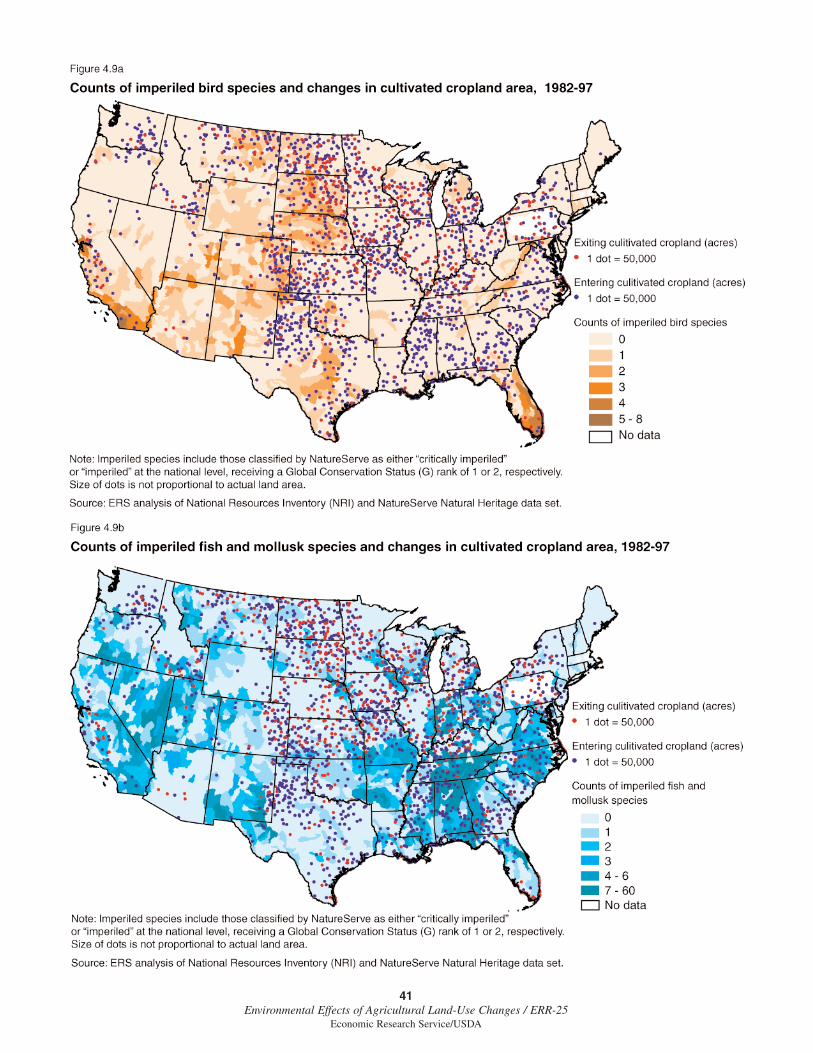
41Environmental Effects of Agricultural Land-Use Changes / ERR-25
Economic Research Service/USDA

also associated with higher levels of potential nutrient loss than are culti-vated croplands that did not change use.
To the extent that particular land-use changes affect particular types ofspecies, a comparison of the location of extensive margin lands and of areaswith high counts of imperiled species could help target conservation policiesor shape government policies that affect land use. Except for CRP enroll-ments, land in cultivated crops moving to and from less intensive uses is inareas with higher overall counts of imperiled animal and plant species.Nevertheless, due to the nature of the imperiled species indicator, we cannotinfer any causal relationships between land-use changes and the imperilmentof species.
The data on cropland transitions from 1982 to 1997 suggest that croplandswith lower soil productivity, which are more likely to be at the extensivemargin, may be more environmentally sensitive in terms of erosion andpotential nutrient loss. Based on soil productivity, lands with lower cropgrowth potential are more susceptible to damage from erosion than are moreproductive lands. While greater erodibility contributes to nutrient loss poten-tial, we lack sufficient data on nutrient applications by lands of differentquality to reach definitive conclusions on the relationship between soilproductivity and nutrient loss.
Lands enrolled in the CRP tend to be different than other lands at the exten-sive margin of cultivated cropland. CRP lands are located in areas withmore erodible land and higher concentrations of imperiled birds (but lowercounts of other imperiled species) than other cropland. Again, it is difficultto make direct comparisons of CRP lands to other lands in the same regionin terms of nutrient loss or species. Broadly speaking, CRP-heavy areas donot appear to be areas where land characteristics and cropping practicescombine to produce above-average nutrient losses.
42Environmental Effects of Agricultural Land-Use Changes / ERR-25
Economic Research Service/USDA

Major agricultural programs that are likely to affect land use include priceand income support (commodity) programs, subsidized crop insurance, andland retirement programs (e.g., the Conservation Reserve Program). Theenvironmental impacts will depend on the location and physical characteris-tics of the lands affected by each policy. Lands enrolling in CRP tend to beless productive and to have different physical characteristics, locations, andenvironmental implications than other lands at the extensive margin of culti-vated crop production. The CRP is an example of a policy that expresslyoffers incentives to take particular types of land out of agricultural produc-tion. The next step in our analysis is to identify the particular lands at theextensive margin potentially brought into production as an unintendedconsequence of Federal farm policies.
While other Federal policies and farm programs could have larger effects oncropland area, we focus on federally subsidized crop insurance for tworeasons. First, this is a large program, and there has been great concernexpressed over the environmental characteristics of lands brought into produc-tion due to such risk-reducing farm programs. In a 1999 letter to Congress, 27conservation and taxpayer groups argued that crop insurance subsidies wouldencourage farmers to cultivate crops in flood- and drought-prone areas andthus promote the conversion of environmentally sensitive forest and pasture-lands to crop production (Environmental Defense, 1999). The contention isthat crop insurance tends to encourage the cultivation of lands that providelow or highly variable crop returns, and that these are the precise areas wherethe environment is particularly sensitive to crop cultivation. For example, inthe context of a different Federal policy, Stavins and Jaffe (1990) found thatFederal flood control projects had the unintended consequence of promotingcropland expansion onto forested wetlands, which are valuable ecosystems forfish and wildlife and important for water quality.
Second, determining how government policies affect land-use changerequires distinguishing the effect of the policy from other factors likechanges in commodity prices. CRP, as a land retirement program, directlyinvolves land-use conversion (we considered CRP as a distinct land use anddirectly examined the characteristics of CRP lands earlier).1 Participation incrop insurance and other Federal farm programs does not directly require achange in land use. Farmers buying crop insurance for a parcel of landmight well cultivate crops there even without the insurance program. About182 million acres were insured in 1997, or 56 percent of total cultivatedcropland in the 48 contiguous States (Glauber and Collins, 2002).
While crop insurance participation does not require land-use conversion,additional analysis might identify unintended land-use impacts from the
1With some caveats, examination ofthe land-use effects of CRP can belargely restricted to those particularlands participating in the program.One caveat is the possibility of “slip-page,” the extent to which croplandretirement under the program might beoffset by consequent reallocations ofother lands outside the program to cul-tivated cropland uses (Wu, 2000;Roberts and Bucholtz, 2005). Thismight be expected if land retirement issignificant enough to alter commodityprices. Another caveat is that CRPlands that would have left crop pro-duction even without the program donot represent cropland retirementsdirectly attributable to CRP. Lubowskiet al., (2003) estimate such lands at 8percent of 1997 CRP acres.
43Environmental Effects of Agricultural Land-Use Changes / ERR-25
Economic Research Service/USDA
Chapter 5
Environmental Effects ofPolicy-Induced Land-Use
Changes

Federal crop insurance program. The large increase in crop insurance subsi-dies after the 1994 Crop Insurance Reform Act can be used as a naturalexperiment to observe how land-use conversions change in response to cropinsurance subsidies. We identify the impact of this policy change bycomparing land-use changes before and after the 1994 Act in response todifferent increases in the expected return to crop insurance. This approachallows us to isolate the impact of the policy change because the sharp reduc-tions in farmers’ insurance costs due to the 1994 Act are likely to be unre-lated to other unobserved factors affecting land use locally.
Analytical Model: The Effect of CropInsurance Subsidies on Land-Use Change
Are the benefits of subsidized crop insurance large enough to affect land-usedecisions? Crop insurance can benefit producers by reducing risk orincreasing returns. If insurance rates are actuarially fair, expected payoutsequal the premiums paid by the beneficiaries. Crop insurance would reducethe variability of returns without changing the average return to cropproduction. In years without losses, insurance costs would lower returnsslightly. In years with indemnified losses, returns would be higher thanwithout insurance due to the insurance payouts. For risk-averse producers,insurance would increase benefits from crop production and couldencourage more cultivation.
Because of information constraints, heterogeneous risks, and other factors,some producers may be charged premiums that are below actuarially fairrates, while others are charged rates above actuarial fairness (Serra et al.,2003; Just et al., 1999; Coble et al., 1996; Vandeveer and Loehman, 1994;Goodwin, 1993). Just et al., (1999) suggest that risk reduction is a minormotive for most crop insurance participants and that most participatingproducers enjoy an increase in average returns over time because subsidiesreduce crop insurance premium rates below actuarially fair levels.
By reducing the risk and/or increasing the expected return from cropproduction, subsidized crop insurance may increase the amount of land incultivated crops. Almost all studies on crop insurance subsidies have notedthe potential for environmental damage due to expanded crop production,particularly if economically marginal land is also more environmentallysensitive. A growing body of literature has focused on the land-use effect ofcrop insurance (Goodwin et al., 2004; Deal, 2004; Goodwin and Smith,2003; Keeton et al., 1999; Wu, 1999; Young et al., 2001; Griffin, 1996), aswell as agricultural disaster payments (Gardner and Kramer, 1986). Thisresearch has chiefly relied on aggregate (county-level) data and has notidentified the environmental characteristics of lands affected by the cropinsurance policies. Previous studies, including one of the few farm-levelanalyses (Wu, 1999), focus on subsets of crops and relatively smallgeographic regions, limiting an assessment of the overall impacts of subsi-dized crop insurance. Most analyses, moreover, do not examine changes incropland over time, making it difficult to distinguish the effect of policiesfrom other factors that could drive land-use decisions in different locations.Finally, some studies use simulation models that hinge on assumptionsabout farmers’ responses to changes in risk (e.g., Young et al., 2001).
44Environmental Effects of Agricultural Land-Use Changes / ERR-25
Economic Research Service/USDA

Since the early 1990s, significant increases in premium subsidies have prob-ably expanded the group of producers with positive expected (average)returns to crop insurance. Our estimates of the impacts of crop insurancesubsidies use data on observed changes in land use on individual landparcels before and after 1994. In that year, the Crop Insurance Act increasedpremium subsidies for all crop insurance products while adding catastrophiccoverage and revenue insurance options. Further premium subsidy increaseswere enacted in 1999-2000. Depending on the level of coverage purchased,subsidies can be as high as 67 percent of producers’ insurance costs, upfrom a maximum of 30 percent prior to 1994, while catastrophic (CAT)coverage is offered for a nominal cost. Crop insurance participation ratesrose with the growth in subsidies (Dismukes and Vandeveer, 2001). Insuredacreage more than doubled from about 90 million to 197 million acresbetween 1990-94 and 1995-99, and then rose to 212 million over 2000-03.Program costs roughly doubled to $1.5 billion a year between 1990-94 and1995-99, and then doubled again (to $3.1 billion) after the Agricultural RiskProtection Act of 2000 (Glauber and Collins, 2002).
Most of the research on crop insurance and land in crop production usesdata that pre-date even the 1994 crop insurance subsidy increases.2 Yet thesesubsidy increases are a natural experiment from which to measure land-usedecisions against an exogenous change in premium rates. Our econometricmodel of land-use change is based on the parcel-specific data on land useand land characteristics from the 1992 and 1997 National Resources Inven-tory (NRI). This period spans the change in expected benefits from cropinsurance resulting from the 1994 Act and allows us to relate changes inland use to changes in the expected benefits from crop insurance. BecauseNRI collects data on the same points of land over time, it is possible todefine gross land-use changes—rather than just net movements—and toidentify the type or quality of land that is actually changing use. Therefore,it is possible to estimate the characteristics, location, and quantity of landbrought into and retained in crop production because of the insurancepremium subsidy increases.
By estimating responses to changes in insurance benefits, we control formany unobserved factors that might also affect the amount of land in cropproduction. The underlying assumption is that regional variation in subsidy-induced changes in insurance benefits are unrelated to other, unobservedfactors driving land use during 1992-97.3
Factors that influence land-use choices include the profitability of alterna-tive land uses, which vary over time and among regions. While we lackinformation on the profitability of different land uses for each parcel of landin the NRI, we do have information on several physical features of eachparcel, including land quality, erodibility, slope, proneness to flooding andlocation. These data can be used as proxies for the profitability of alternativeland uses, as well as for the costs of converting from one land use toanother. The 1996 Federal Agriculture Improvement and Reform (FAIR) Actalso introduced changes to farm programs, which likely affected croplanduse during our period of analysis. We combine NRI’s parcel-specific datawith county-level data on insurance returns, government payments, and theprofitability of alternative land uses to develop an econometric model of
2An exception is the recent studyby Goodwin et al., (2004), whichincludes an analysis of wheat and bar-ley production in the Northern GreatPlains over 1997-98.
3By studying changes in land useover time, our analysis controls forunobserved factors determining the ini-tial disposition of land use across thecountry in 1992. Nevertheless, if therewere different trends in land-use changein different locations and unobservedfactors driving these trends were relatedto changes in the expected benefits fromcrop insurance, this could introduce biasinto our estimates.
45Environmental Effects of Agricultural Land-Use Changes / ERR-25
Economic Research Service/USDA

land-use change that covers the contiguous 48 States (appendix D). Thismodel estimates the probability that an NRI parcel used for either cultivatedcrops or uncultivated crops and pasture moves from its current use to any ofsix major land-use alternatives (cultivated crops, uncultivated crops andpasture, CRP; range, forest, and urban) between 1992 and 1997. This modelshould capture the majority of the changes in cultivated cropland, as transi-tions from uncultivated crops/pasture accounted for 77 percent of theacreage moving to cultivated cropland over 1992-97. (We also estimatedmodels for land used for forests, range, and CRP in 1992, but there were toofew observations to achieve convergence during the bootstrapping runs usedto calculate confidence intervals for the estimates).
Changes in returns to crop insurance are our key explanatory variable andare measured as the change in crop revenue due to insurance programparticipation. This is computed as a weighted average across eight majorcrops (corn, wheat, soybeans, cotton, sorghum, barley, oats, and rice) of the(expected) crop insurance indemnity minus the insurance price faced by thefarmer. This price equals the full crop insurance premium minus thepremium subsidy, which is paid by the government. The expected indemnityis based on an average of indemnity payments over the previous 10 years,by county (see appendix D for more detail).4 Crop insurance program dataare available from USDA’s Risk Management Agency (RMA). Data includetotal indemnities, total premiums, and the subsidy by crop, insuranceproduct, and county.
The change in crop insurance returns is positively related to the likelihoodthat land transitioned to cultivated cropland from another use, and to thelikelihood that land cultivated in 1992 remained cultivated in 1997. To iden-tify the magnitude of these effects, we use the estimates from our econo-metric model to conduct a counterfactual simulation of 1992-97 changes inland use and the resulting 1997 land in each use at every NRI point, underthe assumption that the change in expected crop insurance returns was zero.The difference between land use under this scenario and land use inreality—which reflects the effects of the actual 1992-97 change in insurancereturns—provides an estimate of the land-use effects of the 1994 change incrop insurance premium subsidies.5
Higher Insurance Subsidies Increased1997 Cropland Acreage by Up to 1 Percent
Most researchers who have studied the impact of crop insurance on land usehave found that land-use effects are small, on the order of 1-2 million acres(Goodwin et al., 2004; Young et al., 2001). One study—an unpublishedmanuscript by Keeton et al., (1999)—argues that expansion of crop insur-ance policies during the mid-1990s led to the introduction of 15 million newcropland acres (50 million if land in CRP is included) or about 5 percent ofcultivated cropland.
Our results indicate that the increase in crop insurance subsidies changedland use measurably, but modestly (table 5.1). The change in premiumsubsidies in the mid-1990s increased cultivated cropland area (1997) by anestimated 2.5 million acres, or 0.82 percent, with the bulk of this land (1.8
46Environmental Effects of Agricultural Land-Use Changes / ERR-25
Economic Research Service/USDA
4We focus on buy-up insurance, butalso examined specifications adjustingfor changes in catastrophic insurancecoverage (see appendix C).
5In our analysis, we do not compareland use under the counterfactual sce-nario of no crop insurance subsidyincrease to the observed patterns of landuse reported in the 1997 NRI. Rather,we compare the counterfactual scenarioto land use under a simulated “factual”baseline predicted from our estimatedparameters fitted with the actuallyobserved values for the change in insur-ance returns and all other variables (seeappendix C). In this way, we produceestimates of the land-use impacts of thechange in crop insurance returns that areinternally consistent within the frame-work of the econometric model.
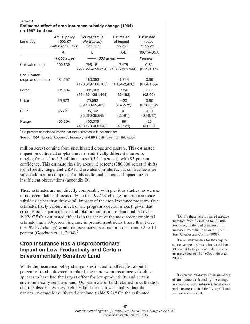
million acres) coming from uncultivated crops and pasture. This estimatedimpact on cultivated cropland area is statistically different than zero,ranging from 1.6 to 3.3 million acres (0.5-1.1 percent), with 95-percentconfidence. This estimate rises by about 12 percent (380,000 acres) if shiftsfrom forests, range, and CRP land are also considered, but confidence inter-vals could not be computed for this additional estimated impact due toinsufficient observations (appendix D).
These estimates are not directly comparable with previous studies, as we usemore recent data and focus only on the 1992-97 changes in crop insurancesubsidies rather than the overall impacts of the crop insurance program. Ourestimates likely capture much of the program’s overall impact, given thatcrop insurance participation and total premiums more than doubled over1992-97.6 Our estimated effect is in the range of the most recent empiricalestimate that a 30-percent increase in premium subsidies (more than twicethe 1992-97 change) would increase acreage of major crops from 0.2 to 1.1percent (Goodwin et al., 2004).7
Crop Insurance Has a DisproportionateImpact on Low-Productivity and CertainEnvironmentally Sensitive Land
While the insurance policy change is estimated to affect just about 1percent of total cultivated cropland, the increase in insurance subsidiesappears to have had the largest effect for low-productivity and certainenvironmentally sensitive land. Our estimate of land retained in cultivationdue to subsidy increases includes land that is lower quality than thenational average for cultivated cropland (table 5.2).8 On the estimated
6During these years, insured acreageincreased from 83 million to 182 mil-lion acres, while total premiumsincreased from $0.7 billion to $1.8 bil-lion (Glauber and Collins, 2002).
7Premium subsidies for the 65-per-cent coverage level were increased from30 percent to 42 percent under the cropinsurance acts of 1994 (Goodwin et al.,2004).
8Given the relatively small numbersof land parcels affected by the changein crop insurance subsidies, local com-parisons are not statistically significantand are not reported.
47Environmental Effects of Agricultural Land-Use Changes / ERR-25
Economic Research Service/USDA
Table 5.1
Estimated effect of crop insurance subsidy change (1994) on 1997 land use
Actual policy Counterfactual Estimated Estimated Land use 1992-97 No Subsidy of impact impact
Subsidy Increase Increase policy of policy
A B A-B 100*(A-B)/A
1,000 acres ––––1,000 acres1–––– Percent1
Cultivated crops 300,639 298,161 2,475 0.82(297,295-299,034) (1,605 to 3,344) (0.53-1.11)
Uncultivatedcrops and pasture 181,257 183,053 -1,796 -0.99
(178,819-180,103) (1,154-2,438) (0.64-1.35)
Forest 391,534 391,668 -134 -03(391,351-391,449) (85-183) (02-05)
Urban 69,672 70,092 -420 -0.60(69,100-69,405) (267-572) (0.38-0.82)
CRP 35,721 35,762 -41 -0.11(35,660-35,669) (22-61) (06-0.17)
Range 400,294 400,379 -85 -02(400,173-400,245) (49-121) (01-03)
1 95-percent confidence interval for the estimates is in parentheses.
Source: 1997 National Resources Inventory and ERS estimates from this study.

48Environmental Effects of Agricultural Land-Use Changes / ERR-25
Economic Research Service/USDA
Table 5.2
Characteristics of additional cropland cultivated due to crop insurancesubsidy increases, relative to CRP and other cropland
Predicted land in Land characteristic cultivation in All cultivated
1997 due to crop cropland in CRP landinsurance subsidy 19971 in 19971
change1
Soil rating for 56.0 60.2 51.3plant growth (SRPG) (55.9-56.1) (60.1-60.3) (51.1-51.5)
% highly erodible land (HEL) 32.3 24.8 56.4(32.2-32.3) (24.5-25.1) (55.9-56.7)
Rainfall erodibility index (EI) 4.89 4.34 7.41(4.82-4.95) (4.29-4.38) (7.30-7.53)
Wind erodibility index (EI) 4.08 3.54 7.24(4.05-4.11) (3.50-3.59) (7.19-7.28)
% Wetland (Cowardin) 2.94 2.44 1.78(2.89-3.0) (2.36-2.52) (1.69-1.88)
% Frequently flooded 1.97 1.81 0.99(1.96-1.99) (1.73-1.88) (0.91-17)
Imperiled animal species 3.11 2.61 2.01(counts/watershed) (3.09-3.12) (2.57-2.65) (1.99-2.03)
Imperiled plant species 3.02 2.14 1.46(counts/watershed) (3.01-3.03) (2.07-2.21) (1.45-1.47)
Imperiled birds species 0.32 0.31 0.39(counts/watershed) (0.32-0.32) (0.31-0.32) (0.39-0.39)
Imperiled fish and mollusk 1.29 1.06 0.81species (counts/watershed) (1.28-1.29) (1.05-1.07) (0.79-0.81
Nitrogen to surface water 11.37 10.57 9.19(1,000 lbs/acre/year) (11.29-11.46) (10.51-10.61) (9.13-9.26)
Nitrogen to estuary 0.51 0.43 0.32(1,000 lbs/acre/year) (0.51-0.52) (0.43-0.44) (0.32-0.32)
Nitrogen leaching 8.90 5.82 4.49(1,000 lbs/acre/year) (8.89-8.91) (5.78-5.88) (4.46-4.52)
Phosphorus to surface water 0.71 0.65 0.61(1,000 lbs/acre/year) (0.71-0.71) (0.65-0.65) (0.61-0.62)1 95-percent confidence interval for the estimates is in parentheses. Confidence intervals forthe predictions (first column) were estimated by bootstrap (see appendix D). Confidence inter-vals for second and third columns based on NRI’s stratified survey design.
Source: 1997 National Resources Inventory (NRI), NatureServe, EPIC-based nutrient indica-tors, Soil Survey Geographic (SSURGO) data set, and ERS estimates from this study.

acres in cultivation due to the increases in insurance subsidies, averagesoil productivity in terms of SRPG was 56, compared with 60 for all culti-vated cropland. While 25 percent of all cultivated cropland was classed ashighly erodible in 1997, an estimated 33 percent of cultivated acreage dueto the increased subsidies was highly erodible land. These differences arestatistically significant (at the 95-percent confidence level) and consistentwith our earlier finding that extensive margin lands are less productive andmore erodible than overall cropland.
Our findings are also consistent with concerns that lands affected by cropinsurance are likely to lie in floodplains and, in the case of wetlands, onenvironmentally sensitive ecosystems. Lands affected by changes in insur-ance subsidies were slightly more prone to frequent flooding and were morelikely to include wetlands than average cultivated cropland (table 5.2).These differences, too, are statistically significant. Total wetlands affectedby the 1992-97 subsidy increase are estimated at 37,000 acres, roughly 0.7percent of the 5.4 million acres of wetlands under crop cultivation. But theaffected wetlands represent about a fifth of the net loss (163,000 acres) innon-Federal wetland area between 1992 and 1997 (USDA/NRCS, 2000).Ending crop production and restoring these wetland acres could make adifference in the overall loss of wetland function. Of course, realizing thesegains may require more than just discontinuing crop production.
With the 1985 Farm Act, the Government made implementing soil conserva-tion measures on highly erodible land (HEL) and avoiding drainage ofwetlands requirements for receiving certain farm program benefits, includingsubsidized crop insurance (Claassen et al., 2004). Our estimated increase incultivated wetlands due to the insurance subsidy change could be due to reten-tion of previously cultivated wetland acres, which were grandfathered into thelaw, rather than to bringing new land into cultivation. The 1996 Farm Act alsoremoved crop insurance from the list of programs subject to conservationcompliance. This change potentially encouraged some crop cultivation onwetlands and HEL by reducing the incentives of insured farmers to not culti-vate these land types. Because the compliance provisions did not change untilApril 1996, however, it is not clear how large an effect this could have had onthe land-use change over 1992-97. Most insured crop producers also receivecommodity payments which would still have triggered a compliance require-ment. As a result, the change in the compliance status of crop insurance mayhave had little impact on cultivated acreage of HEL and wetlands.
Crop insurance subsidies are also estimated to increase cultivation in areassubject to greater potential nutrient losses to water. While our nutrient lossestimates take into account land erodibility, they may not accurately reflectdifferences in fertilizer applications on extensive margin lands. All fournutrient loss indicators are higher, on average, for those croplands estimatedto be in cultivation due to the increase in crop insurance subsidies than forcultivated croplands overall. In contrast, CRP lands have below-averagelevels of potential nitrogen and phosphorus losses.
Given the evidence that crop insurance affects land use on land that is botheconomically and environmentally marginal, larger insurance premiumsubsidies may be offsetting benefits from agri-environmental programs suchas the CRP, as other researchers have suggested (e.g., Goodwin and Smith,
49Environmental Effects of Agricultural Land-Use Changes / ERR-25
Economic Research Service/USDA

2003). That is true to the extent that the land in cultivated crops due to thecrop insurance subsidy increase is also targeted for CRP enrollment. Acresestimated to be in crop cultivation due to crop insurance subsidies and acresenrolled in CRP are both, on average, more erodible and less productivethan overall cropland (table 5.2). A different pattern is evident in the case ofwetlands and land subject to frequent flooding. While the land cultivateddue the increased subsidies is more likely than overall cropland to containthese land types, CRP is less likely to enroll these lands (table 5.2).
Moreover, the location of CRP enrollments differs from that of cultivatedcroplands added from the 1992-97 increase in crop insurance subsidies (fig.5.1). Acres estimated to be in crop cultivation due to crop insurance subsi-dies (the red dots) are clustered in certain regions (Prairie Gateway, Missis-sippi Portal, and Eastern Seaboard) and not uniformly spread through CRPareas (the green dots).
The Heartland (Missouri, Iowa, Illinois, Indiana, Ohio) has extensive croplandand a fair amount of land shifting in and out of cultivated crops. This region,
50Environmental Effects of Agricultural Land-Use Changes / ERR-25
Economic Research Service/USDA

9These estimates account for thefact that the level of participation inthe crop insurance program wasalready high in the Heartland, withless potential for an increase than inregions with historically low participa-tion levels (appendix D).
10For the CRP analysis, we assumethat land area affected by CRP is lim-ited to the enrolled acres (seeAppendix D). Thus, lands not enrolledin CRP in 1997 remain in theirobserved 1997 use in our simulation ofthe environmental impacts in our base-line without the program. Thisassumes no shifts of non-crop landsinto crop production in response toCRP. If such “slippage” is significant,the amount of land enrolled in CRPoverestimates the actual croplandreduced by the program and our esti-mated environmental benefits fromCRP would thus be overstated. Wu(2000) estimated that about 21 acreshave been brought into crop produc-tion for every 100 retired throughCRP. More recent studies using thesame data have found no evidence ofslippage, suggesting that the magni-tude of slippage remains an open ques-tion (Roberts and Bucholtz, 2005).
11Our estimates indicate that annualwind and water erosion in the contigu-ous 48 States in 1997 declined by135.5 and 86.1 million tons, respec-tively, as a result of CRP (table 5.3).These aggregate figures are almostidentical to estimated 1997 reductionsof 134.6 and 89 million tons fromSullivan et al., (2004). The FarmService Agency (FSA) reports annualwind and water reductions from CRPof 241 and 166 million tons for 2000,when overall CRP enrollment was31.4 million acres (USDA/FSA2004a). These reductions are substan-tially larger on a per acre basis thanour estimates. The differences can beaccounted for principally by FSA’sassumption that CRP land would becropped under pre-CRP managementconditions in the absence of the pro-gram. In contrast, our estimates andSullivan et al., 2004 reflect some CRPlands exiting cultivation without theprogram as well as 1997 baseline ero-sion rates, which were significantlylower than 1982 rates for cultivatedcropland (see figs. 3.2 and 3.3).
however, has relatively few CRP lands (except for a cluster in Iowa andNorthern Missouri) and virtually no estimated lands in production due to thechange in crop insurance subsidies. This pattern may be explained by varia-tion in the actuarial performance of the crop insurance program.9 Lands areestimated to have shifted into cultivation as a result of crop insurance in areaswhere crop insurance was a better deal for farmers (e.g., the actuarialperformance was worse). The Federal crop insurance program has historicallyperformed better for corn and soybeans in the Midwest, and more poorly forcotton in the Southern Plains (Young et al., 2001).
Lands Affected by Crop InsuranceSubsidies and Imperiled Species Habitat
Estimated lands in cultivation due to the increase in crop insurance subsi-dies include some areas with high populations of imperiled wildlife species.In particular, the cluster of added lands in the Plains States coincides withan area of high CRP enrollment and high counts of imperiled birds. Addedlands along the Mississippi River and Eastern Seaboard are in watershedsthat overlap with habitats of imperiled fish and mollusks. The landspredicted to be in cultivation due to the increase in crop insurance subsidiesare disproportionately located in watersheds with higher counts of imperiledvertebrates, plants, and fish/mollusks (relative to the average for cultivatedcropland) (table 5.2). In contrast, CRP lands lie in areas with greater countsof imperiled birds (but not of other imperiled species) (table 5.2).
This is consistent with the fact that protecting habitat, particularly for birds,is an express CRP objective. Other areas with relatively high levels ofimperiled species, such as Appalachia, have little or no extensive marginchanges in cultivated cropland (see chapter 4). Available data are not suffi-cient to determine whether observed or predicted land-use changes have animpact (positive or negative) on imperiled wildlife populations.
Crop Insurance Effects on Wind and Water Erosion
Changes in cultivated crop acreage prompted by the increase in crop insur-ance subsidies translate into small aggregate changes in soil erosion, despitehigher levels of erosion per acre than other cropland. While the NRI reportserosion levels given 1997 land use, we estimate erosion under the hypothet-ical scenarios of no insurance subsidy change and no CRP using our econo-metric estimates and erosion data for lands with similar physicalcharacteristics (see appendix E). While land in cultivated crops is estimatedto increase 0.8 percent, wind and water erosion in 1997 are estimated toincrease by 1.4 and 0.9 percent as a result of the increase in insurancepremium subsidies (table 5.3).
This environmental impact is much smaller than that of the 32.7 millionCRP acres enrolled in 1997.10 CRP is estimated to reduce wind erosion 16percent and water erosion 7 percent below the 1997 baseline.11 Since culti-vated cropland enrolled in CRP accounted for about 8 percent of total culti-vated cropland in 1997, the estimated 16-percent reduction in wind erosionis even more notable.12
51Environmental Effects of Agricultural Land-Use Changes / ERR-25
Economic Research Service/USDA

Lands affected by the change in crop insurance subsidies and by CRP aremore susceptible to wind erosion damage than average cultivated cropland,but vulnerability to rainfall erosion appears about average. This is incontrast to other extensive margin lands, which are more susceptible to rain-fall and often wind erosion damage than cultivated cropland overall (seechapter 4). Differences in water erosion are driven largely by slope. Winderosion depends on site-specific conditions as well as climatic factors,which vary regionally. Thus, policy changes, which might target lands inparticular geographical areas, could affect lands that are more vulnerable towind rather than rainfall erosion.
The environmental impacts of the lands affected by the different policiesalso differ. Lands estimated to be brought into or retained in production dueto increased crop insurance subsidies had, on average, higher rates of watererosion but lower rates of wind erosion than lands enrolled in the CRP(table 5.3). This could be due to the greater proportion of acres cultivateddue to the crop insurance subsidy change outside of the Plains, a regionwith above-average wind erosion. This acreage was less vulnerable thanCRP lands in terms of potential nitrogen runoff to surface water, but morevulnerable in terms of potential nitrogen leaching as well as runoff reachingestuaries. This is perhaps due to the greater concentration of lands in culti-vation due to the increase in crop insurance subsidies along the MississippiPortal. Different agricultural and conservation policies thus affect differentsubsets of lands along the extensive margin with different intended—andunintended—environmental implications.
52Environmental Effects of Agricultural Land-Use Changes / ERR-25
Economic Research Service/USDA
12For our erosion calculations, netreductions in cropland for CRP areactually somewhat less than 8 percentas we allow CRP lands to leave cropproduction in the absence of the pro-gram. Thus, the CRP’s per acre reduc-tions in wind and water erosion areeven larger than the reported numbers.
Table 5.3
Estimated erosion impacts of policy-driven land-use changes
Crop insurance subsidy increase Conservation Reserve Program
Environmental Impact on 1997 Impact as % Impact Impact on 1997 Impact as % Impact indicator baseline levels1 of 1997 baseline2 per acre baseline levels1 of 1997 baseline2 per acre
Wind erosion 9,311 1.4 3.8 -135,497 -15.8 -4.1
Water erosion 10,931 0.9 4.5 -86,074 -7.2 -2.61 Erosion values are in 1,000 tons/acre/year.2 Different 1997 baselines are used for the crop insurance and CRP analyses to generate internally consistent estimates for each policy asdescribed in appendix D.
Source: ERS estimates and data from the 1997 National Resources Inventory (NRI).

The links between soil productivity and environmental damages from cropcultivation have important implications for policies that influence land use.The evidence indicates that lands of low agricultural quality are more likelyto move into and out of intensive agricultural uses and are also more sensi-tive environmentally based on some indicators of erosion, nutrient losses towater, and proximity to imperiled species. This suggests that policies thatincrease incentives for crop cultivation and thereby stimulate production oneconomically marginal land will have production effects that are smaller—and environmental impacts that are greater—than would be expected if thesecharacteristics of the affected lands were not accounted for. Conversely,environmental benefits could be achieved at lower cost using targetedconservation programs because owners of low-quality and environmentallysensitive land require less payment to remove land from production thanowners of higher quality land.
Our findings on the land-use and environmental impacts of crop insurancesubsidies and of the Conservation Reserve Program (CRP) are consistentwith the view that government farm programs disproportionately affect landuse in areas that are less productive and more environmentally sensitive insome ways than other croplands. But we find that the lands affected by thechange in crop insurance subsidies and by the CRP differ from each otherand other croplands shifting in and out of production. While governmentpolicies that alter the incentives for crop cultivation are more likely to influ-ence land use on economically marginal croplands, the subset of landsaffected depends on the incentive structure of each program. Which landsare affected determines the size and types of environmental impacts. Identi-fying the lands changing use due to specific policy incentives could helpimprove the effectiveness of future farm programs.
53Environmental Effects of Agricultural Land-Use Changes / ERR-25
Economic Research Service/USDA
Conclusions

Anselin, Luc. 1988. Spatial Econometrics: Methods and Models. KluwerAcademic Publishers: Boston, MA.
Association of American Plant Food Control Officials (AAPFCO). 1998.Commercial Fertilizers, 1997. University of Kentucky: Lexington, KY.
Babcock, Bruce A. and David A. Hennessy. 1996. “Input Demand underYield and Revenue Insurance,” American Journal of AgriculturalEconomics, 78(May): 416-427.
Barbier, Edward B. 1997. “The Economic Determinants of LandDegradation in Developing Countries,” Philosophical Transactions:Biological Sciences, 352(1356): 891-899.
Barlowe, Raleigh. 1958. Land Resource Economics: The Political Economyof Rural and Urban Land Resource Use. Prentice-Hall: Englewood,Cliffs, NJ.
Barnard, Charles H., Gerald Whittaker, David Westenbarger, and MaryAhearn. 1997. “Evidence of Capitalization of Direct GovernmentPayments into U.S. Cropland Values,” American Journal of AgriculturalEconomics, 79(5): 1642-1650.
Bockstael, Nancy E. 1996. “Modeling Economics and Ecology: TheImportance of a Spatial Perspective,” American Journal of AgriculturalEconomics, 78(5): 1168-1180.
Carrion-Flores, Carmen and Elena G. Irwin. 2004. “Determinants ofResidential Land-Use Conversion at the Rural-Urban Fringe.” AmericanJournal of Agricultural Economics, 86(4): 889-904.
Cassman, Kenneth G. 1999. “Ecological Intensification of CerealProduction Systems: Yield Potential, Soil Quality, and PrecisionAgriculture.” Proceedings of the National Academy of Sciences. 96:5952-5959.
Claassen, Roger, Vince Breneman, Shawn Bucholtz, Andrea Cattaneo,Robert Johansson, and Mitch Morehart. 2004. Environmental Compliancein U.S. Agricultural Policy: Past Performance and Future Potential.Agricultural Economic Report No. 832. U.S. Department of Agriculture,Economic Research Service.
Claassen, Roger, and Abebayehu Tegene. 1999. “Agricultural Land UseChoice: A Discrete Choice Approach,” Agricultural and ResourceEconomics Review, 28(1): 26-36.
Coble, K.H., T.O. Knight, R.D. Pope, and J.R. Williams. 1996. “ModelingFarm-Level Crop Insurance Demand with Panel Data,” American Journalof Agricultural Economics 78(May): 439-47.
Deal, John. 2004. “The Empirical Relationship between Federally-Subsidized Crop Insurance and Soil Erosion.” Ph.D. Dissertation. NorthCarolina State University: Raleigh, NC.
54Environmental Effects of Agricultural Land-Use Changes / ERR-25
Economic Research Service/USDA
References

Dismukes, Robert, and Monte Vandeveer. 2001. “U.S. Crop Insurance:Premium, Subsidies, and Participation,” Agricultural Outlook. (Dec.): 21-24
Dobson A.P., J.P. Rodríguez, W.M. Robert, and D.S. Wilcove. 1997.“Geographic Distribution of Endangered Species in the United States,”Science, 275: 550–553
Dubois, Mark R., Kenneth McNabb and Thomas J. Straka. 1999. “CostTrends for Forestry Practices in the South,” Forest Farmer, 32: 3-8.
Ehrenfeld, David, Reed F. Noss, and Gary K. Meffe. 1997. “EndangeredSpecies ‘Hot Spots’: Letters,” Science, 276(5312): 513-517.
Environmental Defense. 1999. “Letter to the U.S. House of Representativesfrom 27 Conservation and Taxpayers Groups Opposing Crop InsuranceBills That Would Spur Excess Cropping, Pesticides and Fertilizer onMarginal Lands.” http://www.environmentaldefense.org/docu-ments/1366_crop%20insurance%20letter2.htm
Feather, Peter, Daniel Hellerstein, and Leroy Hansen. 1999. EconomicValuation of Environmental Benefits and the Targeting of the ConservationPrograms: The Case of the CRP. Agricultural Economics Report No. 778.U.S. Department of Agriculture, Economic Research Service.
Gardner, Bruce L., and Randall A. Kramer. 1986. “An Experience with CropInsurance Programs in the United States,” Crop Insurance for AgriculturalDevelopment: Issues and Experience, P. Hazell, C. Pomerada, and A. Valdez(eds.). Kluwer Academic Publishers: Boston, MA.
Glauber, Joseph W. 2004. “Crop Insurance Reconsidered,” AmericanJournal of Agricultural Economics, 86(5): 1179-1195.
Glauber, Joseph W. and Keith J. Collins. 2002. “Risk Management and theRole of the Federal Government,” A Comprehensive Assessment of theRole of Risk in Agriculture,” Richard E. Just and Rulon E. Pope (eds.).Kluwer Academic Publishers: Boston, MA.
Goodwin, Barry K. 1993. “An Empirical Analysis of Demand for MultiplePeril Crop Insurance,” American Journal of Agricultural Economics,5(May): 425-34.
Goodwin, Barry K., and Vincent H. Smith. 2003. “An Ex Post Evaluation ofthe Conservation Reserve, Federal Crop Insurance, and OtherGovernment Programs: Program Participation and Soil Erosion.,” Journalof Agricultural and Resource Economics, 28(2): 201-216.
Goodwin, Barry K., Monte L. Vandeveer, and John L. Deal. 2004. “AnEmpirical Analysis of Acreage Effects of Participation in the FederalCrop Insurance Program,” American Journal of Agricultural Economics,86(4): 1058-1077.
Greene, William H. 1998. LIMDEP Version 7 Econometric Software, Inc.:Plainview, NY.
Griffin, Peter W. 1996. “Investigating the Conflict in Agricultural PolicyBetween the Federal Crop Insurance and Disaster Assistance Programsand the Conservation Reserve Program.” Ph.D. dissertation, University ofKentucky: Lexington, KY.
55Environmental Effects of Agricultural Land-Use Changes / ERR-25
Economic Research Service/USDA

Hardie, Ian, and Peter Parks. 1997. “Land Use with Heterogeneous LandQuality: An Application of an Area Base Model,” American Journal ofAgricultural Economics, 79(2): 299-310.
Heimlich, Ralph E. 1989. “Productivity of Highly Erodible Cropland,” TheJournal of Agricultural Economics Research, 41(3): 17-22.
Heimlich, Ralph E., and William D. Anderson. 2001. Development at theUrban Fringe and Beyond: Impacts on Agriculture and Rural Land.Agricultural Economic Report No. 803, U.S. Department of Agriculture,Economic Research Service.
Hof, J., C. Flather, T. Baltic, and S. Davies. 1999. “National Projections ofForest and Rangeland Condition Indicators: A Technical DocumentSupporting the 1999 USDA Forest Service RPA Assessment,” GeneralTechnical Report PNW-GTR-442. U.S. Department of Agriculture, U.S.Forest Service. Pacific Northwest Research Station: Portland, OR.
Horowitz, John K., and Erik Lichtenberg. 1993. “Insurance, Moral Hazard,and Chemical Use in Agriculture,” American Journal of AgriculturalEconomics, 75: 425-434.
Irwin, Elena G., Kathleen Bell, and Jacqueline Geoghegan. 2003.“Modeling and Managing Urban Growth at the Rural-Urban Fringe: AParcel-Level Model of Residential Land Use Change,” Agricultural andResource Economics Review, 32(1): 83-102.
Irwin, Elena G. and Nancy E. Bockstael. 2002. “Interacting Agents, SpatialExternalities, and the Endogenous Evolution of Residential Land UsePattern,” Journal of Economic Geography, 2(1).
Just, R.E., L. Calvin, and J. Quiggen. 1999. “Adverse Selection in CropInsurance: Actuarial and Asymmetric Information Incentives,” AmericanJournal of Agricultural Economics 81(Nov.): 834-49.
Kantrud, H.A. 1993. “Duck Nest Success on Conservation Reserve ProgramLand in the Prairie Pothole Region,” Journal of Soil and WaterConservation, 48(3): 238-242.
Keeton, Kara, Jerry Skees, and James Long. 1999. “The Potential Influenceof Risk Management Programs on Cropping Decisions.” Selected paperpresented at the annual meeting of the American Agricultural EconomicsAssociation, Nashville, TN.
Kellogg, R.L., C.H. Lander, D.C. Moffitt, and N. Gollehon. 2000. ManureNutrients Relative to the Capacity of Cropland and Pastureland toAssimilate Nutrients: Spatial and Temporal Trends for the United States.U.S. Department of Agriculture, Economic Research Service and NaturalResource Conservation Service.
Lichtenberg, Erik. 1989. “Land Quality, Irrigation Development, andCropping Patterns in the Northern High Plains,” American Journal ofAgricultural Economics, 71 (Feb.): 187-194.
Long, J. Scott, and Jeremy Freese. 2001. Regression Models for CategoricalDependent Variables Using Stata. Stata Corporation: College Station, TX.
56Environmental Effects of Agricultural Land-Use Changes / ERR-25
Economic Research Service/USDA

Lubowski, Ruben N., Marlow Vesterby, Shawn Bucholtz, Alba Baez, andMichael J. Roberts. 2006. Major Uses of Land in the United States, 2002.Economic Information Bulletin, forthcoming. U.S. Department ofAgriculture, Economic Research Service.
Lubowski, Ruben N., Andrew J. Plantinga, and Robert N. Stavins. 2003.“Determinants of Land-Use Change in the United States, 1982-97:Results from a National Level Econometric and Simulation Analysis.”Resources for the Future Discussion Paper No. 03-47. Washington, DC.
McFadden, Daniel. 1974. “Conditional Logit Analysis of Qualitative ChoiceBehavior,” Frontiers in Econometrics. Paul Zarembka (ed.). AcademicPress. New York, NY.
McMillen, Daniel P. 1992. “Probit with Spatial Autocorrelation,” Journal ofRegional Science, 32(3): 335-348.
Miranowski, John and Brian D. Hammes. 1984. “Implicit Prices of SoilCharacteristics for Farmland in Iowa,” American Journal of AgriculturalEconomics, 66(5): 745-749.
Mitchell, G., R.H. Griggs, V. Benson, and J. Williams. 1998. EnvironmentalPolicy Integrated Climate Model. http://www.brc.tamus.edu/epic.
Moulton, Robert J. and Kenneth R. Richards 1990. Costs of SequesteringCarbon through Tree Planting and Forest Management in the UnitedStates. GTR WO-58. U.S. Department of Agriculture, Forest Service.
Niemuth, Neal. 2004. Problems Associated with Using Opportunistic Datain Assessing Conservation Value of Landscapes for Birds. USFWSHabitat and Population Evaluation Team: Bismarck, ND.
Nusser, S.M., and J.J. Goebel. 1997. “The National Resources Inventory: ALong-Term Multi-Resource Monitoring Programme,” Environmental andEcological Statistics, 4(3): 181-204.
O’Connnor, Raymond J., Malcolm T. Jones, Randall B. Boone, and T. BruceLauber. 1999. “Linking Continental Climate, Land Use, and LandPatterns with Grassland Bird Distribution Across the ConterminousUnited States,” Studies in Avian Biology, 19(1): 45-59.
Pimentel, David, and Nadia Kounang. 1988. “Ecology of Soil Erosion inEcosystems,” Ecosystems, 1: 416-426.
Plantinga, Andrew J. 1996. “The Effects of Agricultural Policies on LandUse and Environmental Quality,” American Journal of AgriculturalEconomics, 78(4): 1082-1091.
Pierce, F.J., W.E. Larson, R.H. Dowdy, and W.A.P. Graham. 1983.“Productivity of Soils: Assessing Long-Term Changes Due to Erosion,”Journal of Soil and Water Conservation, 38(Jan.-Feb.): 39-44.
Quiggin, J., G. Karagiannis, and L. Stanton 1993. “Crop Insurance and CropProduction: An Empirical Study of Moral Hazard and Adverse Selection,”Australian Journal of Agricultural Economics, 37(2): 95-113.
57Environmental Effects of Agricultural Land-Use Changes / ERR-25
Economic Research Service/USDA

Roberts, Michael and Shawn Bucholtz. 2005. “Slippage in the ConservationReserve Program or Spurious Correlation? A Comment,” AmericanJournal of Agricultural Economics, 87(1): 244-250.
Schatzki, Todd. 2003. “Options, Uncertainty, and Sunk Costs: An EmpiricalAnalysis of Land Use Change,” Journal of Environmental Economics andManagement, 46: 86-105.
Serra, Teresa, Barry K. Goodwin, and Allen M. Featherstone. 2003.“Modeling Changes in the U.S. Demand for Crop Insurance During the1990s,” Agricultural Finance Review, 63(Fall): 109-125.
Skidmore, E.L., and N.P. Woodruff. 1968. Wind Erosion Forces in theUnited States and Their Use in Predicting Soil Loss. AgricultureHandbook No. 346. U.S. Department of Agriculture, AgriculturalResearch Service.
Smith, R.A., G.E. Schwarz, and R.B. Alexander. 1997. “RegionalInterpretation of Water-Quality Monitoring Data,” Water ResourcesResearch, 33: 2781-2798.
Smith, Vicent H., and Barry K. Goodwin. 1996. “Crop Insurance, MoralHazard, and Agricultural Chemical Use,” American Journal ofAgricultural Economics, 78: 428-438.
Soil Survey Staff, 2000. Soil Ratings for Plant Growth—A System forArraying Soils According to their Inherent Productivity and Suitabilityfor Crops. C.S. Holzhey and H.R. Sinclair, eds. U.S. Department ofAgriculture, Natural Resources Conservation Service, National SoilSurvey Center. Lincoln, NE.
State of Illinois, Department of Agriculture. 2001. “Farmland Protection.”http://www.agr.state.il.us/Environment/LandWater/farmlandprot.html(revised March 2005)
Stavins, Robert N., and Adam B. Jaffe. 1990. “Unintended Impacts ofPublic Investments on Private Decisions: The Depletion of ForestedWetlands,” American Economic Review, 80(3): 337-352.
Stein, B., L. Kutner, and J. Adams. 2000. Precious Heritage: The Status ofBiodiversity in the United States. Oxford University Press: New York, NY.
Sullivan, Patrick, Daniel Hellerstein, Leroy Hansen, Robert Johansson,Steven Koenig, Ruben Lubowski, William McBride, David McGranahan,Michael Roberts, Stephen Vogel, and Shawn Bucholtz. 2004. TheConservation Reserve Program: Economic Implications for RuralAmerica. Agricultural Economic Report No. 834. U.S. Department ofAgriculture, Economic Research Service.
U.S. Congress, Office of Technology Assessment (OTA). 1995. TargetingEnvironmental Priorities in Agriculture: Reforming Program Strategies.OTA-ENV-640.
U.S. Department of Agriculture (USDA), 1973. “Land CapabilityClassification.” Soil Conservation Service Handbook, No. 210.
58Environmental Effects of Agricultural Land-Use Changes / ERR-25
Economic Research Service/USDA

U.S. Department of Agriculture, Economic Research Service (ERS). 2000.Farm Resource Regions. Agricultural Information Bulletin No. 760. http://www.ers.usda.gov/publications/aib760/
U.S. Department of Agriculture, Farm Service Agency (FSA). 2004a.“Conservation Reserve Program Fiscal Year Summary, 2003.”
U.S. Department of Agriculture, Farm Service Agency (FSA), 2004b.“Conservation Reserve Program Monthly Summary: October 2004.”
U.S. Department of Agriculture, Farm Service Agency (FSA). 2004c.“Conservation Reserve Program Northern Bobwhite Quail HabitatInitiative.” FSA Online Fact Sheet. http://www.fsa.usda.gov/pas/publica-tions/facts/html/quail04.htm (revised 8/11/04).
U.S. Department of Agriculture, National Agricultural Statistical Service(NASS). 1997. Census of Agriculture – 1997, www.nass.usda.gov/census/.
U.S. Department of Agriculture, Natural Resources Conservation Service(NRCS). 2000. Summary Report: 1997 National Resources Inventory(revised December 2000), including associated data files.
U.S. Department of Agriculture, World Agricultural Outlook Board(WAOB). 2001. USDA Agricultural Baseline Projections to 2010, StaffReport WAOB-2001-1, Office of the Chief Economist.
Vandeveer, Monte L. and Edna T. Loehman. 1994. “Farm Response toModified Crop Insurance: A Case Study of Corn in Indiana,” AmericanJournal of Agricultural Economics, 76(Feb.): 128-140.
Venables, W.N., and B.D. Ripley. 1994. Modern Applied Statistics with S-Plus. Springer. New York, NY.
Wischmeier, W.H., and D.D. Smith. 1978. Predicting Rainfall Erosion Losses:A Guide to Conservation Planning. Agricultural Handbook No. 537. U.S.Department of Agriculture, Science and Education Administration.
World Wildlife Fund (WWF). 2005a. “Northern Great Plains: Threats.”http://www.worldwildlife.org/wildplaces/ngp/threats.cfm
World Wildlife Fund (WWF). 2005b. “Southeast Rivers and Streams:Threats to Biodiversity.”http://www.worldwildlife.org/wildplaces/sers/threats.cfm
Wu, JunJie. 1999. “Crop Insurance, Acreage Decisions, and Nonpoint-Source Pollution,” American Journal of Agricultural Economics,81(May): 305-320.
Wu, JunJie. 2000. “Slippage Effects of the Conservation Reserve Program,”American Journal of Agricultural Economics, 82(4): 979-992.
Wu, JunJie and B. Wade Brorsen. 1995. “The Impact of GovernmentPrograms and Land Characteristics on Cropping Patterns,” CanadianJournal of Agricultural Economics, 43(1): 87-104.
Wu, Junjie, Richard M. Adams, and Andrew J. Plantinga. 2004. “Amenitiesin an Urban Equilibrium Model: Residential Development in Portland,Oregon,” Land Economics, 80(1): 19-32.
59Environmental Effects of Agricultural Land-Use Changes / ERR-25
Economic Research Service/USDA

Wu, JunJie and Kathleen Segerson. 1995. “The Impact of Policies and LandCharacteristics on Potential Groundwater Pollution in Wisconsin,.”American Journal of Agricultural Economics, 77(4): 1033-1047.
Young, C. Edwin, Monte Vandeveer, and Randall D. Schnepf. 2001.“Production and Price Impacts of U.S. Crop Insurance Programs,”American Journal of Agricultural Economics, 83(5): 1196-1203.
60Environmental Effects of Agricultural Land-Use Changes / ERR-25
Economic Research Service/USDA

Appendix A—Land-Use Data
To fully investigate the dynamics of land-use change, we use data on grossland-use change, obtained from the National Resource Inventory (NRI). TheNRI is an area-based survey conducted by USDA’s Natural ResourcesConservation Service (NRCS), in cooperation with Iowa State University.NRI provides information on land use, land characteristics, and conservationpractices for about 800,000 points of nonfederal land across all U.S. coun-ties except for Alaska. Because most of the same points were sampled at 5-year intervals, the NRI allows us to investigate gross land-use changes overtime. Since the 1997 survey, the NRI has changed its procedures to samplefewer points annually. Based on the new annual sample, NRCS providesannual estimates of national land use and summary information on selectedland-use transitions.1
Because NRI is a survey rather than a full enumeration of all land, estimatesof land-use change are subject to a small amount of error. For estimates ofland use and land-use change at the regional and national level, these errorsare quite small and are not reported in tables to avoid clutter. In some cases,however, data presented in the form of maps is aggregated to the 8-digitHydrological Unit Code (HUC). In these cases, only estimates that arestatistically different from zero with 90 percent confidence are displayed.
The NRI places land uses into one of 58 categories, with special emphasison classifying various categories of cropland. The NRI aggregates these 58specific land uses into 12 broad land-use categories. We focus on changesbetween four categories: cultivated crops; uncultivated crops; CRP; andgrazing, forest, and other rural land.
Cultivated cropland primarily includes the cropland uses that require moreintensive management and have the potential to yield higher values(although summer fallow and set-aside acres are also included). In contrast,uncultivated cropland primarily includes hay with no rotation, a lower valueand lower intensity use of cropland. Grazing, forest, and other rural landsinclude pasture, range, forestland, and other farm lands such as farmsteads.
61Environmental Effects of Agricultural Land-Use Changes / ERR-25
Economic Research Service/USDA
1Point-level data are publicly avail-able for the 5-year NRI surveys,enabling the analysis of three land-usetransitions for each sample point(1982-87, 1987-92, 1992-97). At thetime of this study, point-level datawere not publicly available for theannual surveys started in 2001.

62Environmental Effects of Agricultural Land-Use Changes / ERR-25
Economic Research Service/USDA
Table A-1
Land-use classifications in this report based on the National Resources Inventory (NRI)
Classification in NRI broad use NRI specific land-usethis report categories categories
Cultivated cropland Cultivated cropland ● Row crops
● Close crops
● Hay with close/row rotation
● Pasture with close/row rotation
● Double-cropped horticulture
● Set-asides, summer fallow,and aquaculture
Uncultivated cropland Uncultivated cropland ● Single-cropped horticulture
● Hay with no rotation
Conservation Reserve Conservation Reserve Conservation Reserve Program (CRP) Program (CRP) Program (CRP)
Grazing, forest, and ● Pasture ● Pastureother rural land ● Rangeland ● Rangeland
● Forestland ● Forests grazed and ungrazed
● Other rural land ● Other farm & rural land
Developed land ● Urban/built-up ● Urban/small built-up
● Rural transportation ● Urban/10 acres or larger
● Rural transportation
Water and Federal land ● Small water areas ● Small & large streams
● Census water areas ● Small & large water bodies
● Federal land ● Federally owned land
Appendix B—EPIC-Based Nutrient Loss Indicators
This appendix describes how indicators for nitrogen and phosphorus loss towater were simulated using the Environmental Policy Integrated ClimateModel (EPIC) for different crop production activities, as well as pastured landor land planted to trees. EPIC is a crop biophysical simulation model that isused to estimate the impact of management practices on crop yields, soilquality, and pollution discharged at the field level (Mitchell et al., 1998). Ituses information on soils, weather, and management practices—includingspecific fertilizer rates—and produces information on crop yields, erosion,and chemical losses—including nitrogen losses—to the environment. Crop-ping and management practices used in the EPIC management files were setconsistent with agronomic practices for highly erodible (HEL) and non-highlyerodible (non-HEL) land in 45 farm production regions (see fig. B-1).
Cropping Enterprises
The National Resources Inventory (NRI) and Agricultural ResourceManagement Surveys (ARMS) were used to identify 62 crop rotationscommonly used throughout the United States and the tillage practicescommonly associated with them. This totaled 623 systems, which includerotations of up to four crops differentiated by up to five tillage practices.Rotations were defined based on the number of crops contained in the crop-ping history. NRI records were divided into regions by overlaying the 26Land Resource Regions onto the 10 Farm Production regions (fig. B-1).Records were then differentiated by HEL or non-HEL. Acreage for eachrotation was then recorded. Tillage practices associated with the rotationsand the acreage devoted to them were derived from the CPS. Crop rotationsas identified through the NRI were used to group the CPS records.
Running EPIC simulations for the predominant systems (and the physicalimpacts of these systems—yields and environmental effects) requiredobtaining all the management information needed to mimic the completeproduction cycle of any crop in a rotation. This included information on allfield operations from pre-planting to post-harvesting (i.e., what occurred,when it occurred, with what type of equipment, and how frequently) andinput levels (i.e., seeding rates, fertilization and liming rates, pesticide appli-cations, etc.) for each crop within a production activity sorted by rotation,tillage practice, and region.
Fertilizer regimes for each crop in a rotation-tillage system were derivedfrom the fertilizer information contained in ARMS. The means for totalquantity of nitrogen (N), phosphate (P), and potash (K) were used to deter-mine how many pounds per acre of N, P, and K to apply to each system.Likewise, liming information was used to determine lime applications. Also,the most frequently occurring month(s) were used to set fertilization date(s).
ARMS data were also used to determine how many field or tillage opera-tions (other than planting, fertilizing, or spraying) occurred for a crop(again, by farm production region, specific to each crop within a rotation-tillage system). The mean number of machinery operations reported in
63Environmental Effects of Agricultural Land-Use Changes / ERR-25
Economic Research Service/USDA

ARMS for that crop (rounding up or down to an integer, according toconvention) was used. Here too, ARMS data determined the most frequentlyoccurring time(s) of field (tillage) operations.
In matching values to NRI observations according to land use, the estimatedEPIC values for land in single-hay rotations were used for uncultivatedcropland, while values for land in all other rotations (including mixed-hayrotations) were assigned to cultivated cropland. Values for pasture land wereused for both pasture and rangeland while values for land in trees were usedfor forests. Idle cropland and forest values were used for CRP landdepending on whether grass/legumes or trees/wildlife cover were reported inthe NRI.
EPIC Model Runs
We generate an array of environmental indicators associated with each cropproduction activity, as well as pastured land or land planted to trees, byrunning EPIC in two steps. The first step conditions the soil, while the nextis used to calculate average rate of discharge. Each step was run to generateseparate environmental values for HEL and non-HEL.
The first or conditioning step allows EPIC to rectify any inconsistencies inthe soil profile imported from STATSGO data set.1 It involves running EPICout for 5-years while keeping its soil erosion module turned off. This stepmakes the soils profile at the next step consistent with a field that has beensubjected to the management practices being simulated. This is importantbecause any particular soil profile used does not necessarily come from afield where the system being simulated has been used.
In the next step, environmental indicators are calibrated by running EPICout for 60 years, this time with soil erosion turned on. Total discharges foreach indicator are tabulated and divided by the length of the simulation toobtain the annual rate of discharge. Running the systems for 60 years doestwo things: it eliminates the dependence of the discharge from the sequenceof weather for any particular period and it provides a consistent base formaking comparisons between systems. By eliminating the dependence onweather, we do not have to coordinate weather patterns among the variousweather sites. Therefore, all systems are run through two full weathercycles. At the same time, each management regime is run through at leastfive full management cycles.
Selected Indicators
We categorize the potential impacts of changes in agricultural productionon nutrients lost to the environment using several indicators. The indica-tors we examine are: nitrogen runoff, nitrogen leaching, nitrogen loss toestuaries, and phosphorus loss to water. Excess nitrogen balance is firstconstructed using data on chemical fertilizer use, manure fertilizer, andnitrogen fixed by legumes. From this, the nitrogen harvested in crop yieldis subtracted, which leaves excess nitrogen left on the field vulnerable toleaching or runoff. Nitrogen runoff is the amount of nitrogen in subsur-face flow, in solution, and attached to sediment that is estimated to arrive
64Environmental Effects of Agricultural Land-Use Changes / ERR-25
Economic Research Service/USDA
1See http://www.ncgc.nrcs.usda.gov/products/datasets/statsgo/metadata/index.html.
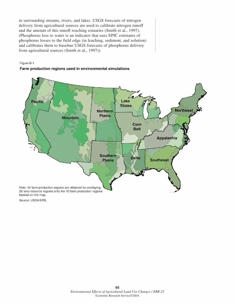
in surrounding streams, rivers, and lakes. USGS forecasts of nitrogendelivery from agricultural sources are used to calibrate nitrogen runoffand the amount of this runoff reaching estuaries (Smith et al., 1997).(Phosphorus loss to water is an indicator that uses EPIC estimates ofphosphorus losses to the field edge (in leaching, sediment, and solution)and calibrates them to baseline USGS forecasts of phosphorus deliveryfrom agricultural sources (Smith et al., 1997)).
65Environmental Effects of Agricultural Land-Use Changes / ERR-25
Economic Research Service/USDA

Appendix C—Imperiled Species Counts
Counts of “imperiled” species are derived from the conservation status rank-ings in NatureServe’s Natural Heritage data set as of 2000, though data fordifferent States may reflect different levels of updating. NatureServe is anonprofit network of biological inventories, known as natural heritageprograms or conservation data centers, in all 50 U.S. States as well as othercountries. The Natural Heritage data set includes conservation status assess-ments of species from all three taxa (animals, invertebrates, and plants) andtheir classes. Data on invertebrates is probably the most incomplete of thethree as heritage programs tend to assign low priority to collecting speciesdata for this group (NatureServe, 2005).
For each species (or “element”) in the Natural Heritage data set, Nature-Serve assigns a ranking of its risk of extinction.1 While NatureServe has awide variety of ranking measures, we use their highest level ranking, theirso-called “G” ranking, which rates the element’s risk of extinction on arangewide or “global” basis. For our analysis, we consider “imperiledspecies” as those classified by NatureServe as either “critically imperiled”or “imperiled” at the national level, receiving a Global Conservation Status(G) rank of 1 or 2, respectively.2
Standard ranking criteria and definitions are used to ensure that a particularrank has the same meaning regardless of the species or geographic regionconsidered. Ranking is a qualitative process based on the following factors:total number and condition of element occurrences, population size, rangeextent and area of occupancy, short- and long-term trends in the foregoingfactors, threats, environmental specificity, and fragility. According toNatureServe, “The ranker’s overall knowledge of the element allows him orher to weigh each factor in relation to the others and to consider all perti-nent information for a particular element” (NatureServe, 2005).3
The set of species identified by the Natural Heritage network as imperiledor vulnerable provides a more accurate indication of biodiversity hot spotsthan the federally maintained endangered species list, according to Ehren-feld et al., (1997). The list of species under the Endangered Species Actincludes only species that are formally designated as endangered or threat-ened as a result of legal proceedings, rather than all species considered bymost biologists to be at risk of extinction (Stein et al., 2000). Additionally,the NatureServe data avoid the problems of raw population occurrence data,which overemphasize areas that have been particularly well inventoried.This is overcome by calculating the number of different species within ageographical unit. Counts of imperiled species also help to overcome incon-sistencies in inventory intensity.
NatureServe data are available at a national level and in a Geographic Infor-mation System (GIS) format. However, these data are often collected withlimited a priori justification, which limits their usefulness because of vari-able sampling efforts, inconsistent sampling protocols, small sample sizes,inclusion of opportunistic observations, and a tendency to report unusualobservations. In addition, species included in data sets often vary amongStates (Niemuth, 2004).
66Environmental Effects of Agricultural Land-Use Changes / ERR-25
Economic Research Service/USDA
1An “element” is defined as a unitof natural biological diversity, repre-senting species, ecological communi-ties, or other nontaxonomic biologicalentities, such as migratory speciesaggregation areas. These elementsrefer to the species records by countyand by watershed only. No ecologicalcommunities or other significant areassuch as migratory stopover points areincluded in the data sets provided.
2An element known or assumed toexist within a jurisdiction is designatedby a whole number from 1 to 5, denot-ing: 1 = critically imperiled; 2 =imperiled; 3 = vulnerable to extirpa-tion or extinction; 4 = apparentlysecure; and 5 = demonstrably wide-spread, abundant, and secure(NatureServe, 2005).3See http://www.natureserve.org/explorer/ranking.htm for more infor-mation.

Appendix D—Estimating Land-Use ChangesFrom Crop Insurance Subsidies
This appendix describes the econometric model used to estimate changes incultivated cropland area resulting from the large increase in crop insurancepremium subsidies during the mid-1990s. Following discrete choice studieson land-use change (e.g., Schatzki, 2003; Lubowski et al., 2003; Irwin andBockstael, 2002; Claassen and Tegene, 1999), the model builds on tradi-tional rent theory to estimate the likelihood that a parcel of land in a partic-ular land use in 1992 remains in the same use or move to a different one by1997. The land-use impact of the increase in crop insurance subsidies isestimated by exploiting variation in the expected profits from crop cultiva-tion due to the large change in premium subsidies from 1992 to 1997. Byexamining changes in land use in relation to changes in subsidies, the effectof the subsidies can be identified, controlling for other determinants of land-use change. A critical assumption is that the policy change is largely exoge-nous and uncorrelated with other, unobserved land-use determinants notincluded in the model.
The likelihood that land transitions from four initial land-use categories(cultivated crops, uncultivated crops or pasture, range, forest) to any of sixbroad land-use options (cultivated crops, uncultivated crops or pasture, CRP,range, forest, and urban) is estimated using observation-specific data onland use and land characteristics from the National Resources Inventory(NRI) and county-level estimates of net returns to the different land-usealternatives.1 One key explanatory variable is the change in expected prof-itability of crop cultivation in a county resulting from the change inpremium subsidies from 1992 to 1997. Estimated parameters from themodel are used to simulate 1997 land use under a hypothetical case inwhich there was no change in crop insurance subsidies over the previous 5years. The difference in 1997 land-use predictions with and without thechange in crop insurance returns provides an estimate for the impact of the1992-97 subsidy increase at the level of each NRI observation.
Conditional Logit Model
We hypothesize that a producer (or other land-use decisionmaker) willchoose to convert a parcel of land from one land use to another based on theprofitability (rents) of the alternative land uses (see chapter 3). If land-usepatterns are initially in equilibrium, then only changes in the relative levelsof profits—and not the profit levels themselves—should drive land-use tran-sitions. Although our focus is on land-use changes over time (1992-97), weinclude 1992 profit levels (as well as the 1992-97 changes in these levels) inour analysis because the levels will matter if land markets were in disequi-librium initially. Because our measures of profits are not normalized to anyone use, we also include profit levels because they indicate the relativeprofits among alternative uses. Relative profits will matter for land-usechanges if hurdles in relative rents must be crossed to induce producers toconvert from one land use to another.
Producers presumably compare net returns to alternative uses on particularland parcels. Although we do not observe profits of alternative land uses for
67Environmental Effects of Agricultural Land-Use Changes / ERR-25
Economic Research Service/USDA
1Uncultivated crops and pastureaccount for the majority of changes toand from cultivated crops. These cate-gories are combined as our estimatesof net returns from these activities arebased on similar factors (hay and for-age prices and yields). We do notmodel land starting in urban uses asthese lands are unlikely to transitionfrom development to agricultural landuses. We also do not examine transi-tions of land exiting CRP, as lands eli-gible to leave the program represent asmall fraction of the land base anddepend on government as well aslandowner choices. These issues areexplored in Sullivan et al., (2004).

each NRI observation, we do observe certain parcel-level attributes andcondition our estimates on these attributes as well as on interactionsbetween the attributes and county-level profits and profit changes. Weinclude these interactions because lands with different attributes may bemore or less likely to convert from one use to another, especially becauseour measures of relative profits are based on relatively coarse county-leveldata. In this way, we model some within-county variation in land-use profitsfrom the different activities. The parcel-level attributes, plus an interceptthat varies by land-use transition, also proxy for the costs of converting landfrom its current use to each of the six land-use alternatives. These attributesinclude point-level indicators of land quality (Land Capability Class), erodi-bility, average slope gradient, and flooding frequency.
Land parcels near one another may have unobserved characteristics thatare correlated across space. If such characteristics influence land-usedecisions or if local land-use choices are interdependent, error terms willbe correlated across space, leading to inconsistent and inefficient esti-mates in a logit model due to induced heteroskedasticity (McMillen,1992). We deal with spatial autocorrelation in two ways. First, and mostimportantly, we randomly select only a single point from each samplingcluster of NRI observations because errors within these points locatednear one another are most likely to be strongly correlated.2 Second, weuse a polynomial spatial trend surface to control for spatial heterogeneity.This approach includes a measure of geographic location as an explana-tory variable and is a common approach in spatial statistics (Venables andRipley 1994). This approach differs from an approach common in theliterature on spatial econometrics, which uses a spatially autorcorrelatederror structure (Anselin, 1988).3
The producer’s profit function may be thought of as including both observedand unobserved components. Using a general random utility expression, theone-period expected net profit (utility) to the producer on parcel i fromswitching from use j to k at time t can be specified as:
where εijkt is a random error term. Assuming that the error terms εijkt areindependent and identically distributed with the type I extreme value distri-bution yields, the probability that parcel i transitions from use j to use kbetween t and t+1 can be written as:
This is the general formulation of a conditional logit model (McFadden,1974).4
We estimated separate models for four starting land-uses j (cultivated crops;uncultivated crops/pasture, forests, and range) that allow for six land-usealternatives k (cultivated crops, uncultivated crops/pasture, CRP, range,forest, and urban).5 Each model is based on the same specification. After
68Environmental Effects of Agricultural Land-Use Changes / ERR-25
Economic Research Service/USDA
ijktijkt XfU ε+= )(
∑==>
=
J
l
ijktijltijkt
ijlt
ijkt
U
UPUU
1)exp(
)exp()Prob(
2The NRI has a stratified samplingdesign. Data on urban and water areasare collected for about 300,000 pri-mary sampling areas varying from 40to 640 acres in size. More detaileddata on land characteristics and use arecollected at two to three sample pointsrandomly selected within each of theseareas (Nusser and Goebel, 1997).
3The spatial trend surface has anadvantage over the spatially autocorre-lated error approach for two reasons:First, it may control for omitted fac-tors associated with space, even ifthey are associated with other covari-ates, whereas the spatial error modelmust assume these are not correlated(i.e., a spatial trend may reduce biasin the estimated coefficients, not justthe standard errors). Second, it ismuch easier to estimate. A limiteddependent variable model with spatialautocorrelation could be estimatedusing simulation methods. However,this is very computationally expensive.Remaining spatial autocorrelation, ifpresent, would bias our standarderrors, but not our estimates.
4The term “conditional” logit or“discrete choice” logit (Greene, 1998)is sometimes used for a logit model inwhich the independent variables varyonly over the choices, in contrast to a“multinomial” logit, in which explana-tory variables vary only over the indi-viduals but not over the choices. Themore general choice model used herehas terms varying over both choicesand individuals and is sometimescalled “McFadden’s choice model” ora “mixed model” (Long and Freese2001).
5While we estimated models forfour starting uses, the discussion inchapter 5 focuses on the results basedon land starting in either cultivatedcrops or in uncultivated crops and pas-ture. We focus on these results sincetransitions from uncultivatedcrops/pasture accounted for the major-ity of transitions to cultivated croplandand because there were too few obser-vations of land-use changes to com-pute confidence intervals (for theestimates) for land starting in eitherforests or range. Transitions fromuncultivated crops/pasture to cultivatedcropland accounted for 77 percent ofall land-use transitions from other usesto cultivated cropland between 1992and 1997.

examining several functional forms for f (X) we chose a linear model thatconsiders all possible two-way interactions between a parcel-level indicatorof land quality, based on the Land Capability Class (LCC),6 and estimatedlevels and changes in levels of land-use profits. Two-way interactionsbetween LCC and the other parcel-level measures are also included, andother explanatory variables (described below) are included without interac-tions.7 Dropping the time subscripts, we specify the component of utilitythat is unique to each alternative k (and initial land use j) as:
CRP participation depends on a different set of decisions than other land-use choices, because enrollment depends on both the producer’s bid, whichincludes a proposed rental rate, and the Government’s choice of whether toaccept the bid, which depends on the environmental characteristics of aparcel as well as the cost. Because the program targets cropland, CRP rentalrates are highly correlated with the profitability of cropping in a givenlocality. We account for the effect of crop net returns on the incentive toremain in cropland. Incentives to enroll in CRP are specified as a functionof LCC, the other parcel-level variables, and a spatial trend surface uniqueto this alternative. Lower land quality as measured by LCC has always beenstrongly associated with program eligibility. We would thus expect greaterenrollment on lower quality lands.
The included variables explain a significant share of the variation in land-usechanges, with pseudo R2 measures ranging from 0.71 to 0.86. The estimatedparameters are consistent with economic intuition, with the profit variables(and changes in profits) for each land-use alternative generally significant andpositively associated with a greater likelihood of moving to each respectiveuse.8 The change in insurance returns is positively related, all else equal, tothe probability of moving to cultivated crops from 1992 to 1997.
Results from counterfactual simulations in which insurance net returns areset to zero are reported in chapter 5. In these simulations, land-use changeprobabilities are estimated for each NRI observation in the sample based onthe estimated parameters. These probabilities are multiplied by the acreageweight for each observation to estimate the amount of land transitioningfrom each initial use to each of the six land-use alternatives. These amountsare used as weights in determining mean land characteristics of acresaffected by the increase in crop insurance subsidies relative to cultivatedcropland overall. Standard errors for the predictions were estimated by boot-strap.9 We resampled an equal number of NRI point/clusters from our mainsample (with replacement) and obtained a new set of estimates and predic-tions. We repeated this exercise 500 times for each of the model equations.
69Environmental Effects of Agricultural Land-Use Changes / ERR-25
Economic Research Service/USDA
6The Land Capability Class is asummary measure of the suitability ofthe land for crop production, based ona ranking of 12 different soil charac-teristics that are critical for crop pro-duction. The overall LCC scoreconsists of the lowest ranking given toany of these 12 soil features based onthe principle that this factor will belimiting for crop production (USDA,1973). Higher LCC ratings indicatepoorer soils for crop production. Toensure sufficient observations in eachLCC category, we combine the eightcategories into three: LCC 1-2; LCC3-4; LCC 5-8.
7The choice of these additional par-cel and county-level variables wasdetermined through a process in whichterms were dropped and added succes-sively in order to minimize the Akaike(1974) information criterion (AIC).
8For brevity, given the large numberof variables and equations, individualparameter estimates are not reportedbut are available from the authorsupon request.
9This procedure enabled the con-struction of confidence intervals forthe estimates based on points startingin either cultivated cropland or unculti-vated cropland/pasture in 1992. Therewere too few observations to achieveconvergence in the bootstrapping runsfor the models based on points startingin either forest or range in 1992, so wewere unable to compute standarderrors for the results from these mod-els. The discussion in chapter 5focuses on the results for which stan-dard errors could be estimated.
,)( 0 cjk
cjk
sjk
sjk
sjk
qjk
sjk
cjk
qjk
sjk
qjk
sjkjkijkijk xxxLCCRLCCLCCUXf βαθβααε +++++=−=
ly.respective level, county and ificparcelspec theat measured variables yexplanatorother
denote and and ; timeat quality of is parcelwhether indicating variable dummya is ; county in use to changes) (and returnsnet are
;parameters are and , intercept; pecificealternativ an is where 0
cjk
sjk
qit
Cjkjkt
xxtqiLCCck
R-s θβαα

Data
The likelihood that a land unit moves from one land use to another is estimatedbased on repeated observations of non-Federal land use from the NationalResources Inventory (NRI). The NRI is a panel survey of land use and landcharacteristics on non-Federal lands conducted at 5-year intervals from 1982 to1997 over the 48 contiguous United States (see chapter 2). Data includeapproximately 844,000 “points,” each representing a land area given by asampling weight that is inversely proportional to the sampling intensity (Nusserand Goebel, 1997). Our analysis is based on a subset of points drawn from the657,781 observations that consist of lands that were in cultivated crops; uncul-tivated crops and pasture; forest; or range in 1992 and any of our six alternativeuses in 1997. We randomly sample from these points so as to include only onepoint in each of our 1982 land-use categories within from each of the NRI’sprimary sampling clusters. This reduces our sample to 83,807 points (23,637observations in cultivated crops, 25,148 in pasture, 23,723 in forest, and 11,299in range). This procedure eliminates parcels located near one another in orderto purge our sample of potential spatial dependence.
Summary statistics are provided for each of our county- and parcel-specificvariables (tables D-1 and D-2). We constructed the land-use profit variables(and changes in these variables) using county-level data derived from anumber of sources to approximate revenues less variable costs for each thesix land-use activities. In addition to our measure of net returns from urbandevelopment, we include the 1990 “urban influence” code for the centroidof each county. This variable is a distance-weighted measure of access topopulation centers based on the 1990 census and is included as an additionalproxy for urban development pressures, given the coarse nature of our urbanprofit estimates (see Heimlich and Anderson, 2001).10
In addition to crop net returns derived from the market, governmentpayments for 1997 are included as a proxy for prior participation in govern-ment commodity programs and the effect of the major regime change thatdecoupled these commodity payments in 1996. The 1996 Federal Agricul-ture Improvement and Reform (FAIR) Act removed most conditions onplantings and conditioned payments on prior planting histories as opposedto current planting decisions. As a result, payments received in 1997 proxyfor program participation prior to 1996.11
Our key explanatory variable is the 1992-97 change in expected net returns tocrop insurance due to the increase in Federal crop insurance premium subsi-dies. The construction of this variable is described below. To control for netreturns to crop insurance in the initial period (1992), we include the county-level share of insurance program participation for the eight major crops consid-ered. Insurance participation is a revealed preference measure that shouldreflect initial differences across the country in the relative returns from insur-ance participation. This also controls for the amount of initial participation,which determines the potential for an increase in participation over 1992-97.
To control for unobserved factors correlated with location, we estimatemodels with a spatial polynomial surface trend. To estimate this trend, weassign to each point a measure of location, proxied by longitude and latitude
70Environmental Effects of Agricultural Land-Use Changes / ERR-25
Economic Research Service/USDA
10Interaction terms between theurban influence code and the urban netreturns (and changes) are alsoincluded.
11The 1996 FAIR Act also introducedloan deficiency payments (LDPs) andmarketing loan gains (MLGs) for graincrops, which had previously only beenavailable for cotton and rice. Ourresults were not affected by the inclu-sion of county-average changes inexpected LDPs as a separate explana-tory variable.

coordinates for the centroid of each NRI polygon.12 We include these coor-dinates (interacted with an alternative-specific constant) singly and in allsecond and third-order interactions.13
County-Level Estimates of Profits (Net Returns)
Crop Net Returns. Data on prices, yields, costs, and acres are used tocompute a weighted county-level average of the net returns per acre for 21major crops. State-level marketing-year-average prices and county-levelyields are from USDA’s National Agricultural Statistics Service (NASS).Producers are assumed to form expectations of future land-use returns basedon current prices and the average of yields over the previous 5 years. Dataon cash costs as a share of revenue at the State and regional level are fromthe Census of Agriculture and the Economic Research Service (ERS).County acreage from NASS and the Census of Agriculture provided weightsfor averaging across individual crops.
Government Payments. County-level estimates of total Federal farmprogram payments per acre are from the Census of Agriculture and includereceipts from deficiency payments, support price payments, indemnityprograms, disaster payments, and payments for soil and water conservationprojects (USDA/NASS, 1997). Payments under the Conservation Reserveand Wetlands Reserve programs are excluded, as the payments measure isintended to only reflect government payments associated with crop produc-tion only, rather than cropland retirement.
Pasture Net Returns. Annual net returns per acre for pasture are estimatedusing pasture yields from the SOILS-5 data set linked to the NRI, Stateprices for “other hay” from NASS, and per-acre costs for hay and other fieldcrops from the Census of Agriculture.
Range Net Returns. Annual net returns per acre for rangeland are computedwith forage yields from SOILS-5 and State-level grazing rates per head forprivate lands from ERS.
Forest Net Returns. We use a 5-percent interest rate to annualize the esti-mated net present value of a weighted average of sawtimber revenues fromdifferent forest types based on prices, yields, costs, and acres. State-levelstumpage prices were gathered from State and Federal agencies and privatedata services. Regional merchantable timber yield estimates for differentforest types were obtained from Richard Birdsey of the U.S. Forest Service.Regional replanting and annual management costs were derived fromMoulton and Richards (1990) and Dubois et al., (1999). The Faustmannformula was used to compute the optimal rotation age, assuming forestsstart newly planted at year zero. County acreage and timber output datafrom the Forest Inventory and Analysis (FIA) and Timber Product Output(TPO) surveys of the U.S. Forest Service provided weights for averagingacross individual forest types and species, respectively.
Urban Net Returns. Annual urban net returns per acre are estimated as themedian value of a recently developed parcel, less the value of structures,
71Environmental Effects of Agricultural Land-Use Changes / ERR-25
Economic Research Service/USDA
12NRI polygons are land areasdefined by the intersections of allcounties and 9-digit watershed classifi-cations. To protect the confidentialityof landowners sampled by the NRI,more specific location indicators arenot publicly available.
13Denoting the location coordinatesas x and y, we include x, y, xx, yy, xy,xxx, yyy, xxy, and xyy as explanatoryvariables.

annualized at a 5-percent interest rate. Median county-level prices forsingle-family homes were constructed from the decennial Census of Popula-tion and Housing Public Use Microdata Samples and the Office of FederalHousing Enterprise Oversight (OFHEO) House Price Index. Regional dataon lot sizes and the value of land relative to structures for single-familyhomes were from the Characteristics of New Housing Reports (C-25 series)and the Survey of Construction (SOC) microdata from the Census Bureau.
Crop Insurance Returns. For the period of years under study, 1992-97, cropinsurance was dominated by actual production history (APH) contracts,although revenue insurance products were introduced in selected counties in1996 and purchase of these products has grown rapidly in the years since.Return to APH crop insurance can be written as:
where Rni is the change in crop revenue due to insurance program participa-tion; Ii is the crop insurance indemnity; ri − si is the (total) crop insurancepremium, si is the premium subsidy (the premium paid by producers is ri)and E is the expectations operator. Also, catastrophic coverage (APH insur-ance with a 50-percent yield guarantee and 100-percent premium subsidy)was introduced in 1995. In 1995, producers participating in farm commodityprograms were required to purchase at least catastrophic coverage(producers where charged a small processing fee, per crop), but the require-ment was dropped for the 1996 and subsequent seasons.
Crop insurance program data for APH contracts, available from USDA’sRisk Management Agency, include total indemnities, total premiums, andthe subsidy by crop and county. To estimate expected returns, expectedindemnity is estimated as the average indemnity over the previous 10 years,by crop and county for eight major crops. A single expected return to cropinsurance is estimated for each county as the acre-weighted average of crop-specific expected returns.
Estimates of expected returns were made with and without catastrophiccoverage. Because our objective was to estimate the impact of the subsidyincreases on expected returns to crop insurance, however, the addition ofcatastrophic coverage confused the situation. While the introduction of cata-strophic coverage significantly increased both liability and enrolled acreage,the low yield guarantee, which made indemnities rare, resulted in a sharpreduction in indemnities per dollar of liability and per unit of land with acrop insurance product. The issues are particularly important given thatcatastrophic coverage was required for the large share of crop producerswho participate in commodity programs. Even when the requirement wasremoved, renewal was automatic and many producers may have simplyallowed the contracts to continue rather than making a conscious decision tocontinue catastrophic coverage. Thus, we believe that the expected return tobuy-up coverage (coverage of 65 percent or higher) best reflects the changein expected returns to crop insurance due to the subsidy increase for thoseproducers who were actually engaged in the crop insurance program.
72Environmental Effects of Agricultural Land-Use Changes / ERR-25
Economic Research Service/USDA
iiini
iiini
srIERE
srIR
+−=
+−=
)()(

73Environmental Effects of Agricultural Land-Use Changes / ERR-25
Economic Research Service/USDA
Table D-1
Summary statistics: County-level variables
County-level variable No. of observations Mean Standard deviation Min. Max
Crop net returns in 1992 ($/acre/year) 657,781 16.9 51.1 -829.2 294.3
Pasture net returns in 1992 ($/acre/year) 657,781 -3.0 76.3 -599.8 200.3
Forest net returns in 1992 ($/acre/year) 657,781 6.9 9.8 -1.2 92.6
Range net returns in 1992 ($/acre/year) 657,781 9.0 10.3 0 73.9
Urban net returns in 1992 ($/acre/year) 657,781 2,224 2,892 183 36,944
Urban influence code in 1990 657,781 1.40 0.89 1.0 5.0
Total government payments in 1997 ($/acre/year) 657,781 8.4 5.9 0 47.3
% of eligible crop acres insured in 1992 657,781 0.4 2.6 0 92
Change insurance net returns, 1992-97 ($/acre/year) 657,781 1.8 4.3 -37.1 40.2
Change in crop net returns, 1992-97 ($/acre/year) 657,781 15.1 62.9 -819.1 939
Change in pasture net returns, 1992-97 ($/acre/year) 657,781 2.2 5.4 -8.2 52
Change in forest net returns, 1992-97 ($/acre/year) 657,781 0.2 2.4 -8.6 12.3
Change in range net returns, 1992-97 ($/acre/year) 657,781 36.2 65.5 -175.2 575.5
Change in urban net returns, 1992-97 ($/acre/year) 657,781 14.1 891 -1,610 10,769
Source: Various sources described in Appendix D.
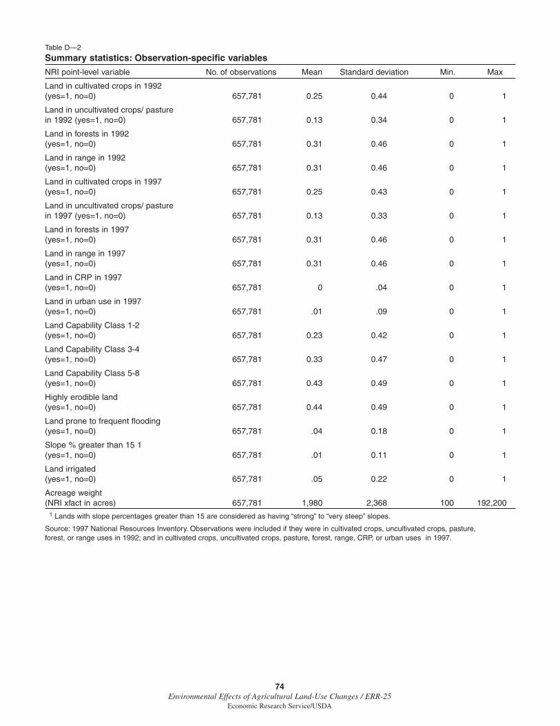
74Environmental Effects of Agricultural Land-Use Changes / ERR-25
Economic Research Service/USDA
Table D—2
Summary statistics: Observation-specific variables
NRI point-level variable No. of observations Mean Standard deviation Min. Max
Land in cultivated crops in 1992(yes=1, no=0) 657,781 0.25 0.44 0 1
Land in uncultivated crops/ pasture in 1992 (yes=1, no=0) 657,781 0.13 0.34 0 1
Land in forests in 1992(yes=1, no=0) 657,781 0.31 0.46 0 1
Land in range in 1992(yes=1, no=0) 657,781 0.31 0.46 0 1
Land in cultivated crops in 1997(yes=1, no=0) 657,781 0.25 0.43 0 1
Land in uncultivated crops/ pasture in 1997 (yes=1, no=0) 657,781 0.13 0.33 0 1
Land in forests in 1997(yes=1, no=0) 657,781 0.31 0.46 0 1
Land in range in 1997(yes=1, no=0) 657,781 0.31 0.46 0 1
Land in CRP in 1997(yes=1, no=0) 657,781 0 .04 0 1
Land in urban use in 1997(yes=1, no=0) 657,781 .01 .09 0 1
Land Capability Class 1-2(yes=1, no=0) 657,781 0.23 0.42 0 1
Land Capability Class 3-4(yes=1, no=0) 657,781 0.33 0.47 0 1
Land Capability Class 5-8(yes=1, no=0) 657,781 0.43 0.49 0 1
Highly erodible land (yes=1, no=0) 657,781 0.44 0.49 0 1
Land prone to frequent flooding (yes=1, no=0) 657,781 .04 0.18 0 1
Slope % greater than 15 1(yes=1, no=0) 657,781 .01 0.11 0 1
Land irrigated (yes=1, no=0) 657,781 .05 0.22 0 1
Acreage weight (NRI xfact in acres) 657,781 1,980 2,368 100 192,200
1 Lands with slope percentages greater than 15 are considered as having “strong” to “very steep” slopes.
Source: 1997 National Resources Inventory. Observations were included if they were in cultivated crops, uncultivated crops, pasture, forest, or range uses in 1992; and in cultivated crops, uncultivated crops, pasture, forest, range, CRP, or urban uses in 1997.

Appendix E—Estimating Erosion FromPolicy-Driven Changes in Land Use
This appendix describes the procedures used to estimate environmentalimpacts in terms of rainfall and wind erosion from the changes in land useinduced by: (1) the change in crop insurance subsidies from 1992 to 1997and (2) the Conservation Reserve Program as of 1997.
Change in Crop Insurance Subsidies. To estimate the impacts from the1992-97 change in subsidies, we compare erosion under the 1997 land useswith and without the change in crop insurance subsidies, as predicted by theeconometric model. Data on rainfall and wind erosion are derived from theNRI. For each NRI point observed in a particular 1997 land use (e.g.,crops), the actual 1997 erosion data from NRI are used to calculate 1997tons/acre of erosion on the fraction of land at that point predicted by themodel to be in that particular use in 1997. For the acreage at that pointpredicted by the model to be in each different use (e.g., pasture), we imputewind (WEQ) and rainfall (USLE) erosion values based on the average 1997erosion values for similar points in that land use in the same Crop ReportingDistrict (CRD). NRI erosion estimates are only available for land in culti-vated crops, uncultivated crops, pasture, and CRP. Erosion on other landuses is assumed to be zero. Given that most changes between the 1997 base-line and no-subsidy-increase scenarios occur at the margin of cultivatedcropland with uncultivated crops, pasture, and CRP, these data shouldaccount for the majority of the erosion differences due to the simulatedchanges in land use.
To impute wind and rainfall erosion, points are matched based on erodibilityindex (EI) quantiles for wind and water, respectively; land capability class(LCC); and 1992 land use. If perfect matches are not available in a partic-ular CRD, we progressively loosen the requirements for similarity—first interms of erodibility, then LCC, then geographic scale, and then land use—until values are imputed for all points.
Conservation Reserve Program. For the 1997 baseline, given by theobserved 1997 pattern of CRP and land use in the NRI, erosion is estimatedwith 1997 WEQ and USLE erosion values from the NRI. For the counter-factual no-CRP scenario, lands not in CRP are assumed to remain in theirobserved 1997 use. This assumes that lands not enrolling in CRP did notchange use in response to the program (no “slippage”). Lands in CRP in1997 are assumed to convert to other land uses (or remain in the same use)in the same proportion as similar lands in the same geographic area over1982-97. We impute 1997 land use—and associated 1997 rainfall and winderosion—by matching each CRP point to similar points in a CRD based onerodibility, LCC, and pre-CRP land use (1982) through the iterative proce-dure described above.
75Environmental Effects of Agricultural Land-Use Changes / ERR-25
Economic Research Service/USDA