envi tutorial
DESCRIPTION
softwareTRANSCRIPT
Tutorials
ENVI Version 3.0December, 1997 EditionCopyright © 1993-1997 Better Solutions Consulting Limited Liability Company, Lafayette, Colorado, USA
Restricted Rights NoticeThe ENVI® software program and the accompanying procedures, functions, and documentation described herein are owned by Better Solutions Consulting Limited Liability Company (BSC). Their use, duplication, and disclosure are subject to the restrictions stated in the ENVI license agreement.
Limitation of WarrantyBetter Solutions Consulting and Research Systems make no warranties, either express or implied, as to any matter not expressly set forth in the license agreement, including without limitation the condition of the software, merchantability, or fitness for any particular purpose.
Neither Better Solutions Consulting or Research Systems shall be liable for any direct, consequential, or other damages suffered by the Licensee or any others resulting from use of the ENVI software package or its documentation.
Permission to Reproduce this ManualPurchasers of ENVI licenses are given limited permission to reproduce this manual provided such copies are for their use with licensed ENVI software only and are not sold or distributed to third parties. All such copies must contain the title page and this notice page in their entirety.
AcknowledgmentsENVI® is a registered trademark of Better Solutions Consulting Limited Liability Company, for the computer program “ENVI” described herein and licensed for distribution by Research Systems, Inc. IDL is a trademark of Research Systems Inc., for the computer program “IDL” described herein. All other brand or product names are trademarks of their respective holders.

Contents
Introduction . . . . . . . . . . . . . . . . . . . . . . . . . . . . . . . . . . . . 1Introducing ENVI....................................................................................................... 1About These Tutorials ................................................................................................ 2Overview of ENVI Tutorials....................................................................................... 2
ENVI Quick Start ................................................................................................. 2ENVI Tutorial #1: Introduction to ENVI ........................................................... 3ENVI Tutorial #2: Multispectral Classification .................................................. 3ENVI Tutorial #3: Image Georeferencing and Registration .............................. 3ENVI Tutorial #4: Mosaicking Using ENVI....................................................... 3ENVI Tutorial #5: Vector Overlay and GIS Analysis ......................................... 3ENVI Tutorial #6: Map Composition Using ENVI ........................................... 4ENVI Tutorial #7: Introduction to Hyperspectral Data and Analysis .............. 4ENVI Tutorial #8: Basic Hyperspectral Analysis ................................................ 4ENVI Tutorial #9: Selected Mapping Methods Using Hyperspectral Data ...... 5ENVI Tutorial #10: Advanced Hyperspectral Analysis ...................................... 5
i
ii Table of Contents
ENVI Tutorial #11: Hyperspectral Signatures and Spectral Resolution........... 5ENVI Tutorial #12: Vegetation Hyperspectral Analysis Case History.............. 5ENVI Tutorial #13: Near-shore Marine Hyperspectral Case History............... 5ENVI Tutorial #14: Multispectral Processing using ENVI’s Hyperspectral Tools6ENVI Tutorial #15: Basic SAR Processing and Analysis.................................... 6ENVI Tutorial #16: Polarimetric SAR Processing and Analysis ....................... 6ENVI Tutorial #17: Analysis of DEMs and TOPSAR ........................................ 6ENVI Tutorial #18: Introduction to ENVI User Functions .............................. 6
Tutorial Data Files ...................................................................................................... 7Mounting the CD-ROM...................................................................................... 7
ENVI Quick Start . . . . . . . . . . . . . . . . . . . . . . . . . . . . . . . . . 9Overview ................................................................................................................... 10
Files Used in This Tutorial ................................................................................ 10Start ENVI................................................................................................................. 10Load a Grayscale Image............................................................................................ 11
Open an Image File............................................................................................ 11Familiarize Yourself with the Displays ............................................................. 11
Apply a Contrast Stretch .......................................................................................... 13Apply a Color Map ................................................................................................... 13Cycle Through all Bands of the Image (Animate) .................................................. 13Load a Color Composite (RGB) Image ................................................................... 14Scatter Plots and Regions of Interest ....................................................................... 14Classify an Image ...................................................................................................... 15Dynamically Overlay One Image over Another...................................................... 16Overlay Vectors on Image and Get Vector Information........................................ 16Finish Up................................................................................................................... 17
Introduction to ENVI . . . . . . . . . . . . . . . . . . . . . . . . . . . . . . 19Overview of This Tutorial ........................................................................................ 20
Files Used in This Tutorial ................................................................................ 20Working with ENVI ................................................................................................. 20
ENVI File Formats ............................................................................................. 21ENVI Windows and Displays............................................................................ 22Menus in ENVI Windows ................................................................................. 24The Available Bands List ................................................................................... 24
Basic ENVI Functions .............................................................................................. 25Start ENVI .......................................................................................................... 25Open an Image File............................................................................................ 25
Table of Contents ENVI Tutorials
Table of Contents iii
Familiarize Yourself with the Displays.............................................................. 25Use the Mouse Button Descriptions ................................................................. 27Display the Cursor Location.............................................................................. 27Display Image Profiles ....................................................................................... 27Perform Interactive Contrast Stretching .......................................................... 28Display Interactive Scatter Plots........................................................................ 30Apply a Filter ...................................................................................................... 31Link Two Displays.............................................................................................. 32Load a Color Image............................................................................................ 33Select Regions Of Interest .................................................................................. 33Annotate the Image............................................................................................ 34Add Grid Lines ................................................................................................... 37Save and Output an Image ................................................................................ 37End the ENVI Session ........................................................................................ 38
Multispectral Classification. . . . . . . . . . . . . . . . . . . . . . . . . 39Overview of This Tutorial ........................................................................................ 40
Files Used in This Tutorial ................................................................................ 40Examine Landsat TM Color Images ........................................................................ 41
Start ENVI .......................................................................................................... 41Open and Display Landsat TM Data ................................................................ 41Review Image Colors ......................................................................................... 42Cursor Location/Value ...................................................................................... 43
Unsupervised Classification ..................................................................................... 44K-Means ............................................................................................................. 44Isodata................................................................................................................. 44
Supervised Classification .......................................................................................... 45Select Training Sets Using Regions of Interest (ROI) ...................................... 45Classical Supervised Multispectral Classification............................................. 46“Spectral” Classification Methods..................................................................... 48Rule Images ........................................................................................................ 50
Post Classification Processing .................................................................................. 52Class Statistics..................................................................................................... 52Confusion Matrix............................................................................................... 53Clump and Sieve ................................................................................................ 54Combine Classes ................................................................................................ 55Edit Class Colors ................................................................................................ 55Overlay Classes ................................................................................................... 55
Classes to Vector Layers............................................................................................ 56Classification Keys Using Annotation ..................................................................... 56
ENVI Tutorials
iv Table of Contents
Image Georeferencing and Registration. . . . . . . . . . . . . . . 59Overview of This Tutorial ........................................................................................ 60
Files Used in This Tutorial ................................................................................ 60Background - Georeferenced Images in ENVI ....................................................... 61Examine Georeferenced Data and Output Image-Map ......................................... 62
Start ENVI .......................................................................................................... 62Open and Display SPOT Data .......................................................................... 62Edit Map Info in ENVI Header......................................................................... 63Cursor Location/Value ...................................................................................... 64Overlay Map Grids ............................................................................................ 64
Image-to-Image Registration................................................................................... 68Open and Display Landsat TM Image File....................................................... 68Display the Cursor Location/Value .................................................................. 68Start Image Registration and Load GCPs ......................................................... 69Edit, On/Off, Delete, Update, and Predict GCPs............................................. 70Warp Images ...................................................................................................... 71Compare Warp Results Using Dynamic Overlays ........................................... 71Examine Map Coordinates................................................................................ 73Close All Files ..................................................................................................... 73
Image-to-Map Registration ..................................................................................... 73Open and Display Landsat TM Image File....................................................... 73Select Image-to-Map Registration and Restore GCPs ..................................... 73Add Map GCPs Using Vector Display of DLGs............................................... 74Warp Image using RST and Cubic Convolution ............................................. 77Display Result and Evaluate using Cursor Location/Value............................. 77Close Selected Files ............................................................................................ 78
IHS Merge of Different Resolution Georeferenced Data Sets................................ 78Display 30 m TM Color Composite ................................................................. 78Display 10 m SPOT Data................................................................................... 78Perform IHS Sharpening................................................................................... 78Display 10 m Color Image................................................................................. 79Overlay Map Grid .............................................................................................. 79Overlay Annotation ........................................................................................... 79Output Image Map ............................................................................................ 80End the ENVI Session........................................................................................ 80
Mosaicking Using ENVI . . . . . . . . . . . . . . . . . . . . . . . . . . . . 81Overview of This Tutorial ........................................................................................ 82Files Used in this Tutorial ........................................................................................ 82Background - Mosaicking in ENVI ......................................................................... 83
Table of Contents ENVI Tutorials
Table of Contents v
General Topics .......................................................................................................... 83Start ENVI .......................................................................................................... 83Preparing Images................................................................................................ 83Histogram Matching.......................................................................................... 84Feathering ........................................................................................................... 86Virtual Mosaics .................................................................................................. 87
Steps for Creating a Pixel-Based Mosaic ................................................................. 87Set up the Mosaicking Dialog............................................................................ 87Import Images .................................................................................................... 88Create Template or Select Apply to Create Output Mosaic ............................ 89
Pixel-based Mosaicking Example............................................................................. 89Position the images for the Pixel-Based Mosaic............................................... 89
Georeferenced Mosaicking Example ....................................................................... 93Create the Georeferenced Mosaic Image .......................................................... 93Optionally Input and Position Images.............................................................. 93View the Top Image and Cutline ...................................................................... 94View the Virtual, Non-Feathered Mosaic......................................................... 94Create the Output Feathered Mosaic ................................................................ 94Some Additional Options in The Mosaicking dialog....................................... 94
Vector Overlay and GIS Analysis . . . . . . . . . . . . . . . . . . . . 97Overview of This Tutorial ........................................................................................ 98Data Sources and Files Used in this Tutorial .......................................................... 98
ESRI Data and Maps Version 1 CD-ROM ....................................................... 98Space Imaging EOSAT CarterraTM Agriculture Sampler Data ....................... 99Required Files ..................................................................................................... 99
Background - Vector Overlay and GIS Concepts in ENVI................................... 100Capabilities ....................................................................................................... 100Concepts ........................................................................................................... 102The Vector Parameters Dialog ........................................................................ 104ENVI Attributes ............................................................................................... 104
Part 1: Stand-Alone Vector GIS in ENVI .............................................................. 105Start ENVI ........................................................................................................ 105Open an ArcView Vector File (Shape File)..................................................... 106Work with Vector Point data .......................................................................... 106Create the USA state boundaries using IDL mapsets..................................... 107Work with Vector Polygon Data ..................................................................... 107Get Vector Information and Attributes .......................................................... 108View Attributes and Point-and-Click Query.................................................. 108Query Attributes .............................................................................................. 109
ENVI Tutorials
vi Table of Contents
Annotate Map Key in Vector Window........................................................... 111Close the windows and all files ....................................................................... 111
Part 2: Combined Raster/Vector Processing Using ENVI.................................... 112Load Image Data to Combined Image/Vector Display ................................. 112Open a Vector Layer and Load to Image Display .......................................... 112Track attributes with cursor............................................................................ 113Heads-up (on-screen) Digitizing .................................................................... 113Edit Vector Layers............................................................................................ 115Query Operations ............................................................................................ 115Vector-to-Raster Conversions ........................................................................ 116Image-Map Output ......................................................................................... 116Close the windows and all files ....................................................................... 117Raster to Vector Conversions.......................................................................... 117Export ROI to Vector Layer ............................................................................ 117Close the windows and all files ....................................................................... 119Export Classification Image to Vector Polygons............................................ 120
Map Composition Using ENVI . . . . . . . . . . . . . . . . . . . . . . . 123Overview of This Tutorial ...................................................................................... 124Files Used in this Tutorial ...................................................................................... 124Background - Map Composition in ENVI............................................................ 124Getting Started........................................................................................................ 124
Start ENVI ........................................................................................................ 125Open and Display Landsat TM Data .............................................................. 125
Image Display and Map Layout ............................................................................. 127Virtual Borders................................................................................................. 127Grids ................................................................................................................. 129Annotation ....................................................................................................... 131Vector Layers.................................................................................................... 136Output .............................................................................................................. 136
Introduction to Hyperspectral Data and Analysis . . . . . . . . 139IOverview of This Tutorial..................................................................................... 140
Files Used in This Tutorial .............................................................................. 140Background: Imaging Spectrometry...................................................................... 141Introduction to Basic ENVI Functionality............................................................ 141
Start ENVI ........................................................................................................ 141Display a Grayscale Image............................................................................... 142Display a Color Image ..................................................................................... 143
Table of Contents ENVI Tutorials
Table of Contents vii
Link Two Displays............................................................................................ 143Extract Spectral Profiles ................................................................................... 144Animate the Data ............................................................................................. 146
Working With Cuprite Radiance Data .................................................................. 148Load AVIRIS Radiance Data ........................................................................... 149Extract Radiance Spectra ................................................................................. 149Compare the Radiance Spectra ....................................................................... 150Load Spectral Library Reflectance Spectra...................................................... 150Compare Image and Library Spectra .............................................................. 151Close the Windows .......................................................................................... 152
Comparison of Radiance and ATREM Reflectance .............................................. 152Continue or Restart ENVI ............................................................................... 153Load Radiance Data and Start the Z Profiler.................................................. 153Load ATREM Apparent Reflectance Data and Start the Z Profiler............... 153Link Images and Compare Spectra ................................................................. 154Close the Windows .......................................................................................... 155
Compare Different Calibrations ............................................................................ 155Background: Calibration ................................................................................. 155Select Calibrated Spectra from Spectral Library............................................. 157Compare Calibrated Spectra ........................................................................... 158Optional: Browse Calibrated Data Files.......................................................... 158Exit ENVI.......................................................................................................... 160
References................................................................................................................ 160
Basic Hyperspectral Analysis. . . . . . . . . . . . . . . . . . . . . . . . 163Overview of This Tutorial ...................................................................................... 164
Files Used in This Tutorial .............................................................................. 164Spectral Libraries, Image Reflectance Spectra, ROIs, and Color Composites ..... 165
Start ENVI and Load AVIRIS data.................................................................. 165Display a Grayscale Image ............................................................................... 165Browse Image Spectra and Compare to Spectral Library .............................. 165Close Windows and Plots ................................................................................ 169Define Regions of Interest ............................................................................... 169Design Color Images to Discriminate Mineralogy......................................... 173Close Plot Windows and ROI Controls .......................................................... 173
2-D Scatterplots ...................................................................................................... 173Examine 2-D Scatterplots ................................................................................ 173Density Slice the Scatterplot ............................................................................ 174Scatterplot Dancing Pixels ............................................................................... 175Image Dancing Pixels....................................................................................... 175
ENVI Tutorials
viii Table of Contents
Scatterplot ROIs............................................................................................... 175Image ROIs....................................................................................................... 176Scatterplots and Spectral Mixing .................................................................... 177Close the Scatterplot ........................................................................................ 177Close Files and Exit ENVI. .............................................................................. 177
References ............................................................................................................... 177
Selected Mapping Methods Using Hyperspectral Data . . . 179Overview of This Tutorial ...................................................................................... 180
Files Used in This Tutorial .............................................................................. 180Removal of Residual Calibration Errors using “Effort” ....................................... 181
Open and Load the 1995 Effort-Corrected Data ........................................... 181Compare ATREM and Effort Spectra............................................................. 182Close All Files, Displays, and Plots ................................................................. 183
Spectral Angle Mapper Classification.................................................................... 184Select Image Endmembers .............................................................................. 186Execute SAM, Resources Permitting .............................................................. 186Select Spectral Library Endmembers .............................................................. 189Review SAM Results ........................................................................................ 191Optional: Generate new SAM Classified Images Using Rule Classifier ........ 192Close Files and Plots ........................................................................................ 193
Spectral Feature Fitting (SFF) and Analysis .......................................................... 193Open and Load the Continuum-Removed Data ........................................... 195Open and Load the 1995 Effort-Corrected Data ........................................... 196Compare Continuum-removed spectra and Effort Spectra.......................... 196Compare Continuum-Removed and Effort Images ...................................... 197Close the Effort Display and Spectral Profile ................................................. 198Open and Load the Spectral Feature Fitting Scale and RMS Images............ 1982-D Scatterplots of SFF Results ....................................................................... 200Spectral Feature Fitting Ratios - “Fit” Images................................................ 200Close Files and Exit ENVI. .............................................................................. 201
References ............................................................................................................... 201
Advanced Hyperspectral Analysis . . . . . . . . . . . . . . . . . . . . 205Overview of This Tutorial ...................................................................................... 206
Files Used in This Tutorial .............................................................................. 206Open and Load the 1995 Effort-Corrected Data ........................................... 207
MNF Transform Data, Endmembers, and Spectral Unmixing............................ 207Background: Minimum Noise Fraction ......................................................... 207
Table of Contents ENVI Tutorials
Table of Contents ix
Open and Load MNF Image............................................................................ 208Compare MNF Images .................................................................................... 209Examine MNF Scatterplots.............................................................................. 209Use Scatterplots to Select Endmembers.......................................................... 209
Pixel Purity Index ................................................................................................... 211Display and Analyze the Pixel Purity Index.................................................... 211Threshold PPI to Regions of Interest .............................................................. 213
n-Dimensional Visualization ................................................................................. 214Compare n-D Data Visualization with 2-D Scatterplot................................. 214Use the n-D Visualizer ..................................................................................... 215Restore n-D Visualizer Saved State ................................................................. 216Paint Your Own Endmembers ........................................................................ 217Link the n-D Visualizer to Spectral Profiles ................................................... 217Collapse Classes in the n-D Visualizer............................................................ 218Export Your Own ROIs ................................................................................... 218Close all Displays and Other Windows........................................................... 219
Matched Filter Background.................................................................................... 219Matched Filter Results ............................................................................................ 219
Open Files and Compare Matched Filter Results........................................... 219Close all Displays and Other Windows........................................................... 220
Background: Unmixing. ......................................................................................... 220What Causes Spectral Mixing.......................................................................... 221Modeling Mixed Spectra ................................................................................. 221Practical Unmixing Methods .......................................................................... 222
Unmixing Results.................................................................................................... 224Open and Display the Unmixing Results........................................................ 224Determine Abundances ................................................................................... 224Display a Color Composite.............................................................................. 224Optional: Perform Your Own Matched Filtering & Spectral Unmixing ...... 225Exit ENVI.......................................................................................................... 225
References................................................................................................................ 226
Hyperpectral Signatures and Spectral Resolution . . . . . . . 227Overview of This Tutorial ...................................................................................... 228Files Used in This Tutorial ..................................................................................... 228Background ............................................................................................................. 229
Spectral Modeling and Resolution .................................................................. 230Case History: Cuprite, Nevada, USA .............................................................. 230
Start ENVI ............................................................................................................... 233Open A Spectral Library File ........................................................................... 233
ENVI Tutorials
x Table of Contents
View Library Spectra .............................................................................................. 233View Landsat TM Image and Spectra.................................................................... 234
Display Reflectance Image............................................................................... 235View GEOSCAN Data ............................................................................................ 235View GER63 Data ................................................................................................... 237View AVIRIS Data .................................................................................................. 239Evaluate Sensor Capabilities Vs ID Requirements ............................................... 240Draw Conclusions .................................................................................................. 240Selected References of Interest ............................................................................... 242
Vegetation Hyperspectral Analysis Case History. . . . . . . . . 245Overview of This Tutorial ...................................................................................... 246
Objectives ......................................................................................................... 246Files Used in This Tutorial ..................................................................................... 246Tasks........................................................................................................................ 248Jasper Ridge Background Materials....................................................................... 249AVIRIS Processing Flow......................................................................................... 253
Near-Shore Marine Hyperspectral Case History . . . . . . . . . 257Overview of This Tutorial ...................................................................................... 258
Objectives ......................................................................................................... 258Files Used in This Tutorial .............................................................................. 258Tasks ................................................................................................................. 259
Moffett Field Site Background............................................................................... 260AVIRIS Processing Flow......................................................................................... 261Selected References ................................................................................................. 265
Multispectral Processing using ENVI’s Hyperspectral Tools 267Overview of This Tutorial ...................................................................................... 268Background............................................................................................................. 268Files Used in This Tutorial ..................................................................................... 269Standard (Classical) Multispectral Image Processing........................................... 270
Start ENVI ........................................................................................................ 270Read TM Tape or CD ...................................................................................... 270Open and Display Landsat TM Data .............................................................. 270Display and Examine a Color Composite Image ........................................... 271Conduct a Ratio Analysis ................................................................................ 271Run Unsupervised Classification (IsoData) ................................................... 273
Table of Contents ENVI Tutorials
Table of Contents xi
Clump and Sieve, Combine Classes ................................................................ 275Annotate and Output Map.............................................................................. 276
Application of ENVI’S Hyperspectral Tools to Multispectral Data Analysis ...... 276Read TM Tape or CD....................................................................................... 276Calibrate TM to Reflectance ............................................................................ 278Display a Color Composite Image and Extract Spectra ................................. 278Run Minimum Noise Fraction (MNF) Transformation ............................... 279Run PPI to Find Endmembers ........................................................................ 281n-D Visualization and Extract Endmembers.................................................. 282Compare Image Spectra to Spectral Library................................................... 285Spectral Angle Mapper Classification ............................................................. 287Linear Spectral Unmixing................................................................................ 288Annotate and Output Map.............................................................................. 292
Summary ................................................................................................................. 292References................................................................................................................ 292
Basic SAR Processing and Analysis . . . . . . . . . . . . . . . . . . . 295Overview of This Tutorial ...................................................................................... 296Files Used in this Tutorial....................................................................................... 296Background ............................................................................................................. 297
Concepts for processing SAR with ENVI ....................................................... 297RadarSat Data................................................................................................... 297Radarsat-Specific Routines added to ENVI 2.5 .............................................. 298
Single-Band SAR Processing Scenario ................................................................... 298Read CEOS Data, Display Data, and Review Quality .................................... 299Review CEOS Header ...................................................................................... 300Remove Speckle using Adaptive Filters .......................................................... 302Density Slice ..................................................................................................... 303Edge Enhancement .......................................................................................... 304Data Fusion ...................................................................................................... 305
Image-Map Output................................................................................................. 306Summary ................................................................................................................. 307
Polarimetric SAR Processing and Analysis . . . . . . . . . . . . . 309Overview of This Tutorial ...................................................................................... 310Files Used in This Tutorial ..................................................................................... 310Background: SIR-C/SAR ........................................................................................ 311Analyzing SIR-C Data............................................................................................. 311
Read a SIR-C CEOS Data Tape ....................................................................... 311
ENVI Tutorials
xii Table of Contents
Multilook SIR-C Data ..................................................................................... 312Synthesize Images - Start The Actual Tutorial Work Here .................................. 313
Display Images ................................................................................................. 315Define ROIs for Polarization Signatures ............................................................... 317Extract Polarization Signatures.............................................................................. 319Use Adaptive Filters................................................................................................ 321
Display the Filter Result .................................................................................. 322Perform Slant-to-Ground Range Transformation ............................................... 323Use Texture Analysis .............................................................................................. 323
Create Color-coded Texture Map................................................................... 324Create an Image-Map for Output.......................................................................... 324
Exit ENVI ......................................................................................................... 325
Analysis of DEMs and TOPSAR . . . . . . . . . . . . . . . . . . . . . . 327Overview of This Tutorial ...................................................................................... 328Files Used in This Tutorial ..................................................................................... 328
Required Files................................................................................................... 328Background - TOPSAR and DEMs ....................................................................... 329
Description of the Dataset............................................................................... 329Displaying the Data and Converting to Physical Parameters .............................. 329
Start ENVI ........................................................................................................ 330View the TOPSAR Headers............................................................................. 330Load and Display the Raw C-Band image ...................................................... 330Load and Display the Raw DEM image.......................................................... 332Convert the C-Band data to Sigma Zero and DEM to meters ...................... 333
Synthesizing the P- and L-band Data .................................................................... 334Analysis of JPL Polarimetric SAR Data ................................................................. 334
General Concepts for processing SAR with ENVI ......................................... 334Polarimetric Analysis ....................................................................................... 337
Displaying and Analyzing DEMs ........................................................................... 339Display the DEM Converted to Meters .......................................................... 340X and Y Elevation Profiles............................................................................... 340Arbitrary Elevation Transect ........................................................................... 341Color Density Slice the DEM .......................................................................... 342Overlay of Elevation Contours........................................................................ 3433-D Perspective Viewing and Image Overlay................................................. 343Generation of Slope, Aspect, and Shaded Relief ............................................ 347
Image-Map Output ................................................................................................ 348Summary................................................................................................................. 348
Table of Contents ENVI Tutorials

Table of Contents xiii
Introduction to ENVI User Functions . . . . . . . . . . . . . . . . . 351Overview of This Tutorial ...................................................................................... 352
Files Used in This Tutorial .............................................................................. 352Background - Programming in ENVI ................................................................... 352User Defined Band Math Routines ........................................................................ 353
Start ENVI ........................................................................................................ 354Open TM Data ................................................................................................. 354Edit the Band Math Function.......................................................................... 354Compile the Band Math Function .................................................................. 355Run the Band Math Function ......................................................................... 355Display the Result............................................................................................. 356Update the Band Math Function .................................................................... 356Compile the Band Math Function .................................................................. 357Display the Result............................................................................................. 358
Creating a User Function ....................................................................................... 358Editing envi.men .............................................................................................. 358Creating an Event Handler .............................................................................. 359
Running the User Function.................................................................................... 362Start ENVI ........................................................................................................ 362Open TM Data ................................................................................................. 362Compile the Event Handler............................................................................. 362Run the Event Handler .................................................................................... 363
Write the Tiling Routines ....................................................................................... 363Creating the Tiling Routine............................................................................. 363Updating the Event Handler ........................................................................... 363Compile the Tile Processing Routine.............................................................. 368Run the Tile Processing Routine ..................................................................... 369Display the Result............................................................................................. 369End the ENVI Session ...................................................................................... 369Notes on Autocompiling ................................................................................. 369
ENVI Tutorials

xiv Table of Contents
Table of Contents ENVI Tutorials

Introduction
Introducing ENVIENVI (the Environment for Visualizing Images) is a state-of-the-art image processing system designed to provide comprehensive analysis of satellite and aircraft remote sensing data. It provides a powerful, innovative, and user-friendly environment to display and analyze images of any size and data type on a wide range of computing platforms.
With its combined file- and band-based approach to image processing, ENVI allows you to work with entire image files, individual bands, or both. When an input file is opened, each spectral band becomes available to all system functions. With multiple input files open, you can easily select bands from different files to be processed together. ENVI also includes tools to extract spectra, use spectral libraries, and to analyze high spectral resolution image datasets such as AVIRIS, GERIS, and GEOSCAN. In addition to its world-class hyperspectral analysis tools, ENVI provides specialized capabilities for analysis of advanced SAR datasets such as JPL’s SIR-C, AIRSAR, and TOPSAR.
1
2 Introduction
ENVI is written entirely in IDL, the Interactive Data Language. IDL is a powerful, array-based, structured programming language that provides integrated image processing and display capabilities and an easy to use GUI toolkit. ENVI is available as ENVI (offering full ENVI command line capabilities) and ENVI RT (the runtime version of ENVI). The only difference between ENVI and ENVI RT is that ENVI RT does not provide user access to the underlying IDL environment. You will not be able to complete the User Function tutorial provided here if you are running ENVI RT.
About These TutorialsThis document contains hands-on tutorials designed to help you become familiar with ENVI’s features and capabilities. Each tutorial is formatted to clearly direct you through required tasks.
Within each tutorial, the tasks you will perform have been broken down into numbered steps, which appear in bold print. Optional steps and single-step activities are preceded by a text bullet. The following formatting conventions will help you identify the type of action required within the various steps:
• The titles of pulldown menu items appear italicized. They will be connected in order of selection by an “->”. For example, select File -> Open Image File.
• “Button” menus, found in many dialogs, appear in quotes.
• Text boxes, toggle buttons, and other button widgets also appear in quotes.
At the beginning of each tutorial, you will find a detailed outline of the topics covered in that tutorial. Each tutorial begins with an overview and background explaining the history and application of the functions you will be using. Also included are the names of the files required to complete the tutorial.
Finally, at the end of each tutorial, references are provided for further exploration.
Overview of ENVI Tutorials
ENVI Quick StartThis tutorial, which is also distributed as a small booklet with the ENVI CD-ROM is designed to get you quickly into the basics of ENVI. It allows you to start ENVI, load either a grayscale or color image, and apply contrast stretches. It demonstrates image animation (movies) and 2-dimensional scatterplots to help users determine the spectral variability of their data. Regions of Interest (ROI)
About These Tutorials ENVI Tutorials
Introduction 3
selection instructions allow new users to quickly move into multispectral classification. ENVI’s dynamic overlay capabilities are used to compare color composites and classified images. Finally, the tutorial provides a quick introduction to ENVI’s vector overlays and GIS analysis capabilities.
ENVI Tutorial #1: Introduction to ENVIThis tutorial provides basic information about ENVI and some suggestions for your initial investigations of the software. Landsat TM data of Canon City, Colorado are used. This tutorial is designed to introduce first-time ENVI users to the basic concepts of the package and to explore some of its key features. It assumes that you are already familiar with general image-processing concepts.
ENVI Tutorial #2: Multispectral ClassificationThis tutorial leads you through typical multispectral classification procedures using Landsat TM data from Canon City, Colorado. Results of both unsupervised and supervised classifications are examined and post classification processing including clump, sieve, combine classes, and accuracy assessment are discussed. It is assumed that you are already generally familiar with multispectral classification techniques.
ENVI Tutorial #3: Image Georeferencing and RegistrationThis tutorial provides basic information about Georeferenced images in ENVI, and Image-to-Image and Image-to-Map Registration using ENVI. Landsat TM and SPOT data from Boulder, Colorado are used. The tutorial covers step-by-step procedures for successful registration, discusses how to make image-maps using ENVI and illustrates the use of multi-resolution data for image sharpening. The exercises are designed to provide a starting point to users trying to conduct image registration. They assume that you are already familiar with general image-registration and resampling concepts.
ENVI Tutorial #4: Mosaicking Using ENVIThis tutorial is designed to give you a working knowledge of ENVI's image mosaicking capabilities. It uses AVIRIS data from Death Valley, Nevada. Pixel-based mosaicking demonstrates ENVI’s virtual mosaic concept and easy-to-use mosaic tool. Georeferenced mosaicking shows ENVI’s automatic placement of map-referenced images and cutline feathering. The exercises assume that you are already generally familiar with mosaicking techniques.
ENVI Tutorial #5: Vector Overlay and GIS AnalysisThis tutorial introduces ENVI’s vector overlay and GIS analysis capabilities. Stand-alone GIS analysis is demonstrated using ESRI-provided GIS data,
ENVI Tutorials Overview of ENVI Tutorials

4 Introduction
including input of ArcView shapefiles and associated .dbf attribute files, display in vector windows, viewing/editing of attribute data, point-and-click spatial query, and math/logical query operations. Part 2 of this tutorial demonstrates use of ENVI’s combined image display/vector overlay and analysis capabilities using a simulated 4-meter resolution Space Imaging/EOSAT multispectral dataset of Gonzales, California, USA. Data courtesy of Space Imaging/EOSAT. The exercise includes cursor tracking with attribute information, point-and-click query, and heads-up digitizing and vector layer editing. Also demonstrated are generation of new vector layers using math/logical query operations and raster-to-vector conversion of ENVI Regions of Interest (ROI) and/or classification images. Finally, the exercise demonstrates ENVI’s vector-to-raster conversion, using vector query results to generate ROIs for extraction of image statistics and area calculations. It is assumed that the user already as a basic grasp of GIS analysis concepts.
ENVI Tutorial #6: Map Composition Using ENVIThis tutorial is designed to give you a working knowledge of ENVI's map composition capabilities. It uses Landsat TM data of Yellowstone National Park, Wyoming, USA to show creation of an image-map with virtual borders, latitude/longitude and map coordinate grids, map key and scale, declination diagram, image insets, and text annotation.
ENVI Tutorial #7: Introduction to Hyperspectral Data and AnalysisThis tutorial is designed to introduce you to the concepts of Imaging Spectrometry, hyperspectral images, and to selected spectral processing basics using ENVI. For this exercise, we use Airborne Visible/Infrared Imaging Spectrometer (AVIRIS) data of Cuprite, Nevada, USA, to familiarize you with spatial and spectral browsing of imaging spectrometer data and then compare the results of several reflectance calibration procedures.
ENVI Tutorial #8: Basic Hyperspectral AnalysisThis tutorial is designed to introduce you to the concepts of Spectral Libraries, Region of Interest (ROI) extraction of spectra, Directed Color composites, and to the use of 2-D scatterplots for simple classification. We use 1995 Airborne Visible/Infrared Imaging Spectrometer (AVIRIS) apparent reflectance data of Cuprite, Nevada, USA, to extract ROIs for specific minerals, compare them to library spectra, and design R, G, B color composites to best display the spectral information. You will also use 2-D scatterplots to locate unique pixels, interrogate the data distribution, and perform simple classification.
Overview of ENVI Tutorials ENVI Tutorials
Introduction 5
ENVI Tutorial #9: Selected Mapping Methods Using Hyperspectral DataThis tutorial is designed to introduce you to advanced concepts and procedures for analysis of imaging spectrometer data or hyperspectral images. You will use the 1995 Airborne Visible/Infrared Imaging Spectrometer (AVIRIS) data from Cuprite, Nevada, USA, to investigate the unique properties of hyperspectral data and how spectral information can be used to identify mineralogy. You will evaluate “Effort” “polished” spectra vs ATREM-calibrated data, and review the Spectral Angle Mapper classification. You will compare apparent reflectance spectra and continuum-removed spectra. You will also compare apparent reflectance images and continuum-removed images and evaluate Spectral Feature Fitting results.
ENVI Tutorial #10: Advanced Hyperspectral AnalysisThis tutorial is designed to introduce you to additional advanced concepts and procedures for analysis of imaging spectrometer data or hyperspectral images. You will use the 1995 AVIRIS data from Cuprite, Nevada, USA, to investigate sub-pixel properties of hyperspectral data and advanced techniques for identification and quantification of mineralogy. You will use “Effort” “polished” ATREM-calibrated data, and review matched filter and spectral unmixing results.
ENVI Tutorial #11: Hyperspectral Signatures and Spectral ResolutionThis tutorial compares spectral resolution for several different sensors and the effect of resolution on the ability to discriminate and identify materials with distinct spectral signatures. The tutorial uses TM, GEOSCAN, GER63, and AVIRIS data from Cuprite, Nevada, USA, for intercomparison and comparison to materials from the USGS Spectral library.
ENVI Tutorial #12: Vegetation Hyperspectral Analysis Case HistoryThis tutorial presents a case history for use of hyperspectral techniques for vegetation analysis using 1997 AVIRIS data from Jasper Ridge, California, USA. You will run through a complete example using a selection of ENVI’s available tools to produce image-derived endmember spectra and image maps.
ENVI Tutorial #13: Near-shore Marine Hyperspectral Case HistoryThis tutorial presents a case history for use of hyperspectral techniques for analysis of near-shore marine environments using 1994 AVIRIS data from Moffett Field, California, USA. You will run through a complete example using a selection of ENVI’s available tools to produce image-derived endmember spectra and image maps.
ENVI Tutorials Overview of ENVI Tutorials
6 Introduction
ENVI Tutorial #14: Multispectral Processing using ENVI’s Hyperspectral Tools
This tutorial is designed to show you how ENVI’s advanced hyperspectral tools can be used for improved analysis of multispectral data. Landsat TM data from the Bighorn Basin, Wyoming, USA, are used. You view results from a classical multispectral analysis approach, and then will run through a complete example using a selection of ENVI’s available tools to produce image-derived endmember spectra and image maps. To gain a better understanding of the hyperspectral concepts and tools, please run the ENVI hyperspectral tutorials.
ENVI Tutorial #15: Basic SAR Processing and AnalysisThis tutorial is designed to give you a working knowledge of ENVI's basic tools for processing single-band SAR data (such as RadarSat, ERS-1, JERS-1). A subset of Radarsat data from Bonn, Germany, are used to demonstrate concepts for processing SAR with ENVI including image display and contrast stretching, removing speckle using adaptive filters, density slicing, edge enhancement and image sharpening, data fusion, and image-map output.
ENVI Tutorial #16: Polarimetric SAR Processing and AnalysisThis tutorial demonstrates the use of ENVI’s polarimetric radar data analysis functions. It uses Spaceborne Imaging Radar-C (SIR-C) data obtained over Death Valley, California, USA, during the April 1994 mission of the Space Shuttle Endeavor to demonstrate concepts such as multilooking, image synthesis from complex scattering matrix data, selection and display of polarizaton and/or multifrequency images, slant-to-ground range conversion, adaptive filtering, and texture analysis.
ENVI Tutorial #17: Analysis of DEMs and TOPSARThis tutorial uses polarimetric SAR data and a Digital Elevation Model (DEM) generated from JPL’s TOPSAR (interferometric SAR) data for Tarrawarra, Australia. Data Courtesy of JPL. The exercise demonstrates display and analysis of the SAR data and of the DEM using standard tools within ENVI. DEM analysis includes grayscale and color-density-sliced display; generation and overlay of elevation contours, use of ENVI’s X, Y, and arbitrary profiles (transects) to generate terrain profiles; generation of slope, aspect, and shaded relief images; and 3-D perspective viewing and image overlay.
ENVI Tutorial #18: Introduction to ENVI User FunctionsThis tutorial provides basic information on programming in ENVI. It covers the basics for creating user defined band math functions and Plug-in functions, including creating compound widgets and writing data tiling operations. This
Overview of ENVI Tutorials ENVI Tutorials
Introduction 7
tutorial assumes that you are familiar with the “Interactive Data Language (IDL)” and understand how to write functions and procedures in IDL. ENVI RT users cannot program in ENVI, so only the Band Math portion of this tutorial is applicable to these users.
Tutorial Data FilesData files for these tutorials are contained in subdirectories of the ENVIDATA directory of the ENVI Data CD-ROM. Because the data sets are quite large— more than 500 MB of data are included—you may wish to load the files into ENVI directly from the CD-ROM rather than transferring the files to your hard disk. You will obtain better performance, however, if you copy the files to your disk. The specific files used by each exercise are described at the beginning of the individual tutorials.
In the tutorials, we use the term tutorial data directory to refer to the place where the tutorial data sets are stored. Depending on your system and whether you choose to copy the data sets to your hard disk, this could be the data directory on the ENVI CD-ROM “ENVIDATA”, a directory containing links to the ENVI CD-ROM (on some Unix systems), or a place on your hard disk.
Mounting the CD-ROMIn order to have access to the ENVI tutorial data files, you must have a CD-ROM drive connected to your computer or accessible on a network.
UnixPlace the ENVI CD-ROM in your CD-ROM drive and use the Unix mount command to mount the CD-ROM device as a part of the Unix file system. Procedures for mounting devices vary for different platforms; consult the ENVI for Unix Installation Guide if you are not sure how to mount the CD-ROM. Note that on most Unix systems, you must be root to mount the CD-ROM.
Note We suggest that you mount the CD-ROM device in the directory /cdrom. If you choose to mount the CD-ROM in another directory, substitute that directory name for occurrences of /cdrom in these tutorials. Also, not all Unix systems will read the CD-ROM the same way.
WindowsPlace the ENVI CD-ROM in your CD-ROM drive. You can now access the contents of the CD-ROM as if it were another hard drive connected to your system.
ENVI Tutorials Tutorial Data Files

8 Introduction
MacintoshPlace the ENVI CD-ROM in your CD-ROM drive. The ENVI CD-ROM icon should appear on your desktop. You can now access the contents of the CD-ROM as if it were another hard drive connected to your system.
Tutorial Data Files ENVI Tutorials
ENVI Quick StartThe following topics are covered in this tutorial:
Overview ................................................................................................................10Start ENVI ...............................................................................................................10Load a Grayscale Image ..........................................................................................11Apply a Contrast Stretch .........................................................................................13Apply a Color Map..................................................................................................13Cycle Through all Bands of the Image (Animate) ....................................................13Load a Color Composite (RGB) Image.....................................................................14Scatter Plots and Regions of Interest .......................................................................14Classify an Image ....................................................................................................15Dynamically Overlay One Image over Another........................................................16Overlay Vectors on Image and Get Vector Information ............................................16Finish Up ................................................................................................................17
9
10 ENVI Quick Start
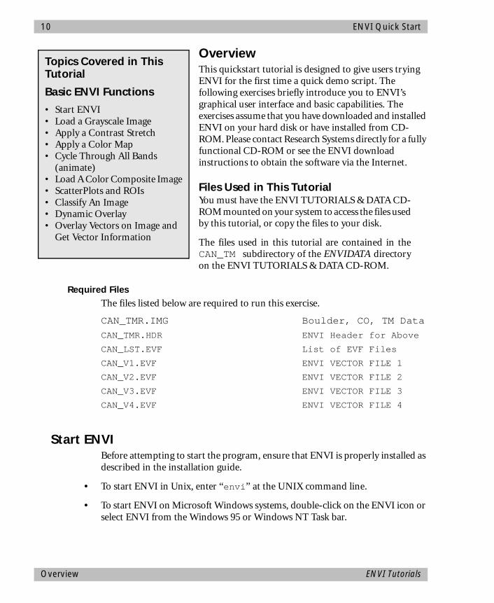
OverviewThis quickstart tutorial is designed to give users trying ENVI for the first time a quick demo script. The following exercises briefly introduce you to ENVI’s graphical user interface and basic capabilities. The exercises assume that you have downloaded and installed ENVI on your hard disk or have installed from CD-ROM. Please contact Research Systems directly for a fully functional CD-ROM or see the ENVI download instructions to obtain the software via the Internet.
Files Used in This TutorialYou must have the ENVI TUTORIALS & DATA CD-ROM mounted on your system to access the files usedby this tutorial, or copy the files to your disk.
The files used in this tutorial are contained in theCAN_TM subdirectory of the ENVIDATA directoryon the ENVI TUTORIALS & DATA CD-ROM.
Required FilesThe files listed below are required to run this exercise.
CAN_TMR.IMG Boulder, CO, TM Data
CAN_TMR.HDR ENVI Header for Above
CAN_LST.EVF List of EVF Files
CAN_V1.EVF ENVI VECTOR FILE 1
CAN_V2.EVF ENVI VECTOR FILE 2
CAN_V3.EVF ENVI VECTOR FILE 3
CAN_V4.EVF ENVI VECTOR FILE 4
Start ENVIBefore attempting to start the program, ensure that ENVI is properly installed as described in the installation guide.
• To start ENVI in Unix, enter “envi” at the UNIX command line.
• To start ENVI on Microsoft Windows systems, double-click on the ENVI icon or select ENVI from the Windows 95 or Windows NT Task bar.
Topics Covered in This Tutorial
Basic ENVI Functions
• Start ENVI• Load a Grayscale Image• Apply a Contrast Stretch• Apply a Color Map• Cycle Through All Bands
(animate)• Load A Color Composite Image• ScatterPlots and ROIs• Classify An Image• Dynamic Overlay• Overlay Vectors on Image and
Get Vector Information
Overview ENVI Tutorials
ENVI Quick Start 11
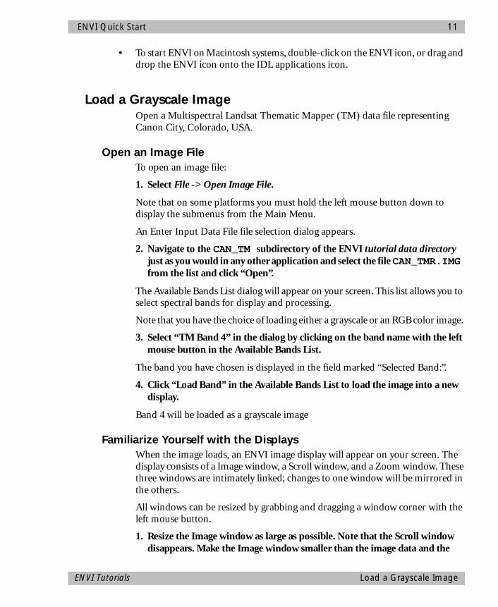
• To start ENVI on Macintosh systems, double-click on the ENVI icon, or drag and drop the ENVI icon onto the IDL applications icon.
Load a Grayscale ImageOpen a Multispectral Landsat Thematic Mapper (TM) data file representing Canon City, Colorado, USA.
Open an Image FileTo open an image file:
1. Select File -> Open Image File.
Note that on some platforms you must hold the left mouse button down to display the submenus from the Main Menu.
An Enter Input Data File file selection dialog appears.
2. Navigate to the CAN_TM subdirectory of the ENVI tutorial data directory just as you would in any other application and select the file CAN_TMR.IMG from the list and click “Open”.
The Available Bands List dialog will appear on your screen. This list allows you to select spectral bands for display and processing.
Note that you have the choice of loading either a grayscale or an RGB color image.
3. Select “TM Band 4” in the dialog by clicking on the band name with the left mouse button in the Available Bands List.
The band you have chosen is displayed in the field marked “Selected Band:”.
4. Click “Load Band” in the Available Bands List to load the image into a new display.
Band 4 will be loaded as a grayscale image
Familiarize Yourself with the DisplaysWhen the image loads, an ENVI image display will appear on your screen. The display consists of a Image window, a Scroll window, and a Zoom window. These three windows are intimately linked; changes to one window will be mirrored in the others.
All windows can be resized by grabbing and dragging a window corner with the left mouse button.
1. Resize the Image window as large as possible. Note that the Scroll window disappears. Make the Image window smaller than the image data and the
ENVI Tutorials Load a Grayscale Image

12 ENVI Quick Start
Scroll window reappears. Try resizing the Zoom window and note how the outlining box changes in the Image window.
The following describes the basic characteristics of the ENVI display group windows:
Image WindowThe Image window shows a portion of the image at full resolution. The zoom control box (the highlighted box in the Image window) indicates the region that is displayed in the Zoom window.
2. To reposition the magnified region, position the mouse cursor in the zoom control box, hold down the left mouse button, and move the mouse. Alternately, you can reposition the cursor and click the middle mouse button to move the magnified area instantly.
Note: On Microsoft Windows systems with a two button mouse, click Ctrl-LeftMouse Button to emulate the middle mouse button.
Note: On Macintosh systems, click Option-Mouse Button to emulate the middlemouse button.
Scroll Window The Scroll window displays the entire image at reduced resolution (subsampled). The subsampling factor is listed in parentheses in the window Title Bar at the top of the image. The highlighted box indicates the area shown at full resolution in the Image window.
3. Move the mouse cursor and click the middle mouse button in the Scroll Windows to reposition the displayed area, or drag with the left mouse button as described above.
Zoom Window The Zoom window shows a portion of the image, magnified the number of times indicated by the number in parentheses in the Title Bar of the window. The zoom area is indicated by a highlighted box (the zoom control box) in the Image window.
4. Click the right mouse button in the Zoom Window to zoom in (increase the magnification).
5. Click the left mouse button in the Zoom Window to zoom out (decrease the magnification).
6. Move the mouse cursor in the Zoom window and click the middle mouse button to reposition the magnified area by centering the zoomed area on the selected pixel.
Load a Grayscale Image ENVI Tutorials

ENVI Quick Start 13
ENVI Tutorials Apply a Contrast Stretch
Display Functions MenuThe Functions menu gives you access to many ENVI features that relate directly to the images in the display group.
7. Click the right mouse button in the Image window to toggle the Functions menu button on and off.
Note: On Macintosh systems, click Command-Mouse Button to simulate theright mouse button.
Apply a Contrast StretchBy default, ENVI displays images with a 2% linear contrast stretch.
1. To apply a different contrast stretch to the image, select Functions->Display Enhancements->Default (quick) Stretches to display a list of default stretching options for each of the windows in the display group.
2. Select an item from the list to apply a contrast stretch to one of the windows.
Alternatively, you can define your contrast stretch interactively by selecting Functions->Display Enhancements->Interactive Stretching in the Image window.
Apply a Color MapBy default, ENVI displays images using a grayscale color table.
1. To apply a pre-defined color table to the image, select Functions->Color Mapping->ENVI Color Tables to display the ENVI Color Tables dialog.
2. Select a color table from the list at the bottom of the dialog to change the color mapping for the three windows in the display group.
Note: On 24-bit color systems you must click the Apply button at the bottom ofthe dialog to apply the selected color table to the image.
3. Select Options->Reset Color Table to return the display group to the default grayscale color mapping.
4. Select File->Cancel to dismiss the Color Tables dialog, keeping your changes.
Cycle Through all Bands of the Image (Animate)You can display all the bands in an image sequentially, creating an animation.
1. Select Functions->Interactive Analysis->Animation and click "OK" in the Animation Input Parameters dialog.

14 ENVI Quick Start
Each of the bands six bands from the TM scene are loaded into a small animation window. Once all the bands are loaded, the images are displayed sequentially as a “movie”.
2. You can control the animation using the CD-Player-like controls in the upper left of the Animation Controls dialog, or the speed of the display by adjusting the "Animation Speed" slider in the upper right of the dialog.
3. Click "Cancel" to end the animation.
Load a Color Composite (RGB) ImageENVI allows simultaneous multiple grayscale and RGB Color displays.
1. To load a color composite (RGB) image of the Canon City area, click on the Available Bands List. If you dismissed the Available Bands List during the previous exercises, you can recall it by selecting File->Available Bands List from the Main ENVI menu.
2. Click on the "RGB Color" radio button in the Available Bands List. Red, Green, and Blue fields appear in the center of the dialog.
3. Select Band 7, Band 4, and Band 1 sequentially from the list of bands at the top of the dialog by clicking on the band names.
The band names are automatically entered in the Red, Green, and Blue fields.
4. Click "Load RGB" to load the image into the Image window.
Scatter Plots and Regions of InterestScatter plots allow you to quickly compare the values in two spectral bands simultaneously. ENVI Scatterplots allow quick 2-band classification.
1. To display the distribution of pixel values between band one and band four of the image as a scatter plot, select Functions->Interactive Analysis->2-D Scatter Plots.
The Scatter Plot Band Choice dialog appears.
2. Under "Choose Band X" select Band 1. Under "Choose Band Y" select Band 4. Click "OK" to create the scatter plot.
3. Place the cursor in the Image window, then press and hold the left mouse button and move the cursor around in the window.
Load a Color Composite (RGB) Image ENVI Tutorials

ENVI Quick Start 15
Notice that as you move the cursor, different pixels are highlighted in the scatter plot. This "dancing pixels" display highlights the 2-band pixel values found in a 10-pixel by 10-pixel region around the cursor.
4. Define a Region of Interest in the Scatter Plot by clicking the left mouse button several times in the Scatter Plot window to select points forming the vertices of a polygon, then clicking the right mouse button to close the polygon.
Pixels in the Image and Zoom windows whose values match the values contained in the selected region of the scatter plot are highlighted.
5. To define a second class, select a second color from the Class menu of the Scatter Plot window and repeat the above steps.
6. Select "Export Class" from the Options menu in the Scatter Plot window to export the most recently created classification. The Region of Interest Controls dialog appears.
By default, ENVI chooses "Scatter Plot Import", followed by the color of the region and number of points contained in the region as the name for the region of interest. This shows up in the "Regions of Interest Controls dialog”.
7. Click "Cancel" to dismiss the dialog. The region definition is saved in memory for the duration of the ENVI session.
Classify an ImageENVI provides two types of unsupervised classification and several types of supervised classification. The following is an example of one of the supervised classification methods.
1. Select Classification->Supervised->Parallelepiped from the ENVI Main menu. When the Classification Input File dialog appears; select CAN_TMR.IMG and click "OK".
2. When the Parallelepiped Parameters dialog appears, select the regions of interest you created from the "Select Classes from Regions" list at the left of the dialog.
3. Select "Output Result to Memory" in the upper right corner of the dialog.
4. Click on the small arrow button in the right-center of the Parallelepiped Parameters dialog to toggle off Rule Image generation, and then click "OK".
ENVI Tutorials Classify an Image
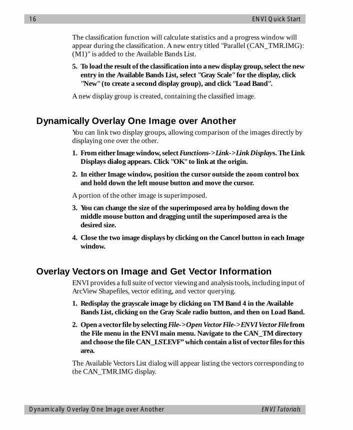
16 ENVI Quick Start
The classification function will calculate statistics and a progress window will appear during the classification. A new entry titled "Parallel (CAN_TMR.IMG): (M1)" is added to the Available Bands List.
5. To load the result of the classification into a new display group, select the new entry in the Available Bands List, select "Gray Scale" for the display, click "New" (to create a second display group), and click "Load Band".
A new display group is created, containing the classified image.
Dynamically Overlay One Image over AnotherYou can link two display groups, allowing comparison of the images directly by displaying one over the other.
1. From either Image window, select Functions->Link->Link Displays. The Link Displays dialog appears. Click "OK" to link at the origin.
2. In either Image window, position the cursor outside the zoom control box and hold down the left mouse button and move the cursor.
A portion of the other image is superimposed.
3. You can change the size of the superimposed area by holding down the middle mouse button and dragging until the superimposed area is the desired size.
4. Close the two image displays by clicking on the Cancel button in each Image window.
Overlay Vectors on Image and Get Vector InformationENVI provides a full suite of vector viewing and analysis tools, including input of ArcView Shapefiles, vector editing, and vector querying.
1. Redisplay the grayscale image by clicking on TM Band 4 in the Available Bands List, clicking on the Gray Scale radio button, and then on Load Band.
2. Open a vector file by selecting File->Open Vector File->ENVI Vector File from the File menu in the ENVI main menu. Navigate to the CAN_TM directory and choose the file CAN_LST.EVF” which contain a list of vector files for this area.
The Available Vectors List dialog will appear listing the vectors corresponding to the CAN_TMR.IMG display.
Dynamically Overlay One Image over Another ENVI Tutorials

ENVI Quick Start 17
3. Click on the“Select All Layers” near the bottom of the dialog to choose the vectors to plot. Click on the “Load Selected” button at the bottom of the Available Vectors List and the Load Vector Layer dialog appears. Click on “Display #1” at the top of the dialog, and then OK.
The vector layers are listed in the Display #1 Vector Parameters dialog.
4. Click on Apply in the Display #1 Vector Parameters dialog to load the vectors onto the image, then choose Options->Vector Information to start an information dialog about the vectors.
5. Click and drag with the left mouse button in the Main Image Display to track the currently selected vector layer and list basic information about the vectors. Click on another layer name in the Vector Parameters dialog and then in the Main Image Display to track a different layer.
Finish Up1. To finish your ENVI session, click "Exit" on the ENVI main menu.
All files will be closed automatically.
ENVI Tutorials Finish Up

18 ENVI Quick Start
Finish Up ENVI Tutorials

ENVI Tutorial#1
Introduction to ENVI
The following topics are covered in this tutorial:
Overview of This Tutorial ........................................................................................20Working with ENVI..................................................................................................20Basic ENVI Functions...............................................................................................25
19
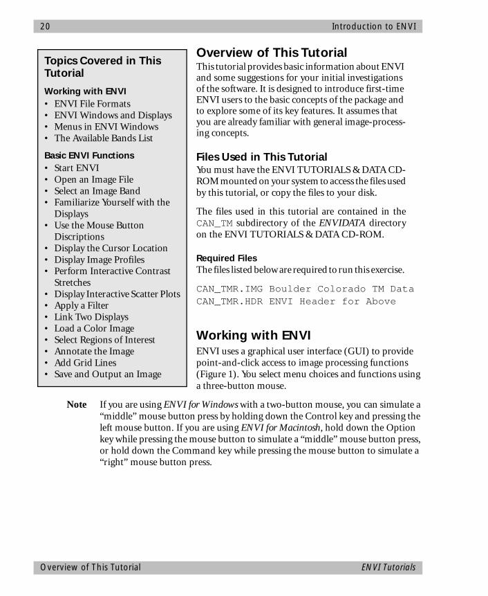
20 Introduction to ENVI
Overview of This TutorialThis tutorial provides basic information about ENVI and some suggestions for your initial investigations of the software. It is designed to introduce first-time ENVI users to the basic concepts of the package and to explore some of its key features. It assumes that you are already familiar with general image-process-ing concepts.
Files Used in This TutorialYou must have the ENVI TUTORIALS & DATA CD-ROM mounted on your system to access the files usedby this tutorial, or copy the files to your disk.
The files used in this tutorial are contained in theCAN_TM subdirectory of the ENVIDATA directoryon the ENVI TUTORIALS & DATA CD-ROM.
Required FilesThe files listed below are required to run this exercise.
CAN_TMR.IMG Boulder Colorado TM DataCAN_TMR.HDR ENVI Header for Above
Working with ENVIENVI uses a graphical user interface (GUI) to provide point-and-click access to image processing functions (Figure 1). You select menu choices and functions using a three-button mouse.
Note If you are using ENVI for Windows with a two-button mouse, you can simulate a “middle” mouse button press by holding down the Control key and pressing the left mouse button. If you are using ENVI for Macintosh, hold down the Option key while pressing the mouse button to simulate a “middle” mouse button press, or hold down the Command key while pressing the mouse button to simulate a “right” mouse button press.
Topics Covered in This Tutorial
Working with ENVI• ENVI File Formats• ENVI Windows and Displays• Menus in ENVI Windows• The Available Bands List
Basic ENVI Functions• Start ENVI• Open an Image File• Select an Image Band• Familiarize Yourself with the
Displays• Use the Mouse Button
Discriptions• Display the Cursor Location• Display Image Profiles• Perform Interactive Contrast
Stretches• Display Interactive Scatter Plots• Apply a Filter• Link Two Displays• Load a Color Image• Select Regions of Interest• Annotate the Image• Add Grid Lines• Save and Output an Image
Overview of This Tutorial ENVI Tutorials
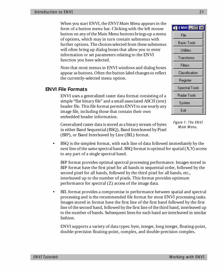
Introduction to ENVI 21
When you start ENVI, the ENVI Main Menu appears in the form of a button menu bar. Clicking with the left mouse button on any of the Main Menu buttons brings up a menu of options, which may in turn contain submenus with further options. The choices selected from these submenus will often bring up dialog boxes that allow you to enter information or set parameters relating to the ENVI function you have selected.
Note that most menus in ENVI windows and dialog boxes appear as buttons. Often the button label changes to reflect the currently-selected menu option.
ENVI File FormatsENVI uses a generalized raster data format consisting of a simple “flat binary file” and a small associated ASCII (text) header file. This file format permits ENVI to use nearly any image file, including those that contain their own embedded header information.
Generalized raster data is stored as a binary stream of bytes in either Band Sequential (BSQ), Band Interleaved by Pixel (BIP), or Band Interleaved by Line (BIL) format.
• BSQ is the simplest format, with each line of data followed immediately by the next line of the same spectral band. BSQ format is optimal for spatial (X,Y) access to any part of a single spectral band.
BIP format provides optimal spectral processing performance. Images stored in BIP format have the first pixel for all bands in sequential order, followed by the second pixel for all bands, followed by the third pixel for all bands, etc., interleaved up to the number of pixels. This format provides optimum performance for spectral (Z) access of the image data.
• BIL format provides a compromise in performance between spatial and spectral processing and is the recommended file format for most ENVI processing tasks. Images stored in format have the first line of the first band followed by the first line of the second band, followed by the first line of the third band, interleaved up to the number of bands. Subsequent lines for each band are interleaved in similar fashion.
ENVI supports a variety of data types: byte, integer, long integer, floating-point, double-precision floating-point, complex, and double-precision complex.
Figure 1: The ENVI Main Menu.
ENVI Tutorials Working with ENVI
22 Introduction to ENVI
The separate text header file provides information to ENVI about the dimensions of the image, any embedded header that may be present, the data format, and other pertinent information. The header file is normally created (with your input) the first time a particular data file is read by ENVI. You can view and edit it at a later time using the Edit ENVI Header function under the ENVI File menu. You can also generate ENVI header files outside ENVI, using a text editor, if desired.
ENVI Windows and DisplaysAs you work with ENVI, a number of different windows and dialog boxes will appear on your screen. These allow you to manipulate and analyze your image. The most important of these displays is a group of three windows that display your image, allow you to move around in it, and allow you to magnify different areas. This group of windows is collectively referred to as the “Display group” (Figure 2). The Display group consists of:
• The Main Display Window - this is where all or part of your image is displayed at full resolution.
• The Scroll Window - If your entire image does not fit in the Main window, the Scroll window will appear. The Scroll window displays a reduced-size version of the entire image, which allows you to select the portion that is displayed in the Main window. A colored box in the Scroll window indicates the spatial location and coverage of the Full-Resolution Main Display window. A number in the title bar of the Scroll Window tells you what reduction factor has been applied to the image to display the full spatial extent within the Scroll Window.
• The Zoom Window - this window displays an enlarged version of a selected portion of the Main window. A colored box in the Main Image Display indicates the spatial location and coverage of the Zoom window. A number in the title bar of the Zoom Window tells you what zoom factor has been applied to the image.
You may have any number of displays open on the screen at any time. There are a wide variety of other types of ENVI windows you may work with, including scatter plots, spectral profiles and spectral plots, and vector windows.
Working with ENVI ENVI Tutorials
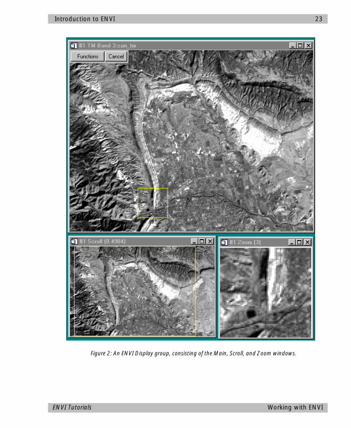
Introduction to ENVI 23
ENVI Tutorials Working with ENVI
Figure 2: An ENVI Display group, consisting of the Main, Scroll, and Zoom windows.
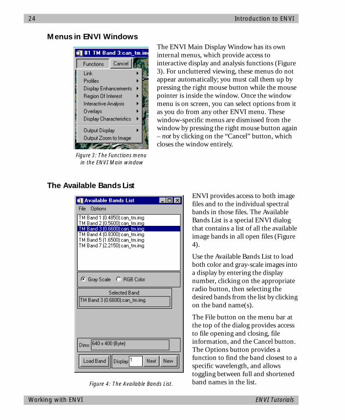
24 Introduction to ENVI
Menus in ENVI WindowsThe ENVI Main Display Window has its own internal menus, which provide access to interactive display and analysis functions (Figure 3). For uncluttered viewing, these menus do not appear automatically; you must call them up by pressing the right mouse button while the mouse pointer is inside the window. Once the window menu is on screen, you can select options from it as you do from any other ENVI menu. These window-specific menus are dismissed from the window by pressing the right mouse button again – not by clicking on the “Cancel” button, which closes the window entirely.
The Available Bands ListENVI provides access to both image files and to the individual spectral bands in those files. The Available Bands List is a special ENVI dialog that contains a list of all the available image bands in all open files (Figure 4).
Use the Available Bands List to load both color and gray-scale images into a display by entering the display number, clicking on the appropriate radio button, then selecting the desired bands from the list by clicking on the band name(s).
The File button on the menu bar at the top of the dialog provides access to file opening and closing, file information, and the Cancel button. The Options button provides a function to find the band closest to a specific wavelength, and allows toggling between full and shortened band names in the list.
Figure 3: The Functions menu in the ENVI Main window
Figure 4: The Available Bands List.
Working with ENVI ENVI Tutorials
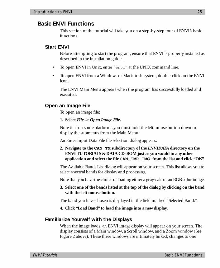
Introduction to ENVI 25
Basic ENVI FunctionsThis section of the tutorial will take you on a step-by-step tour of ENVI’s basic functions.
Start ENVIBefore attempting to start the program, ensure that ENVI is properly installed as described in the installation guide.
• To open ENVI in Unix, enter “envi” at the UNIX command line.
• To open ENVI from a Windows or Macintosh system, double-click on the ENVI icon.
The ENVI Main Menu appears when the program has successfully loaded and executed.
Open an Image FileTo open an image file:
1. Select File -> Open Image File.
Note that on some platforms you must hold the left mouse button down to display the submenus from the Main Menu.
An Enter Input Data File file selection dialog appears.
2. Navigate to the CAN_TM subdirectory of the ENVIDATA directory on the ENVI TUTORIALS & DATA CD-ROM just as you would in any other application and select the file CAN_TMR.IMG from the list and click “OK”.
The Available Bands List dialog will appear on your screen. This list allows you to select spectral bands for display and processing.
Note that you have the choice of loading either a grayscale or an RGB color image.
3. Select one of the bands listed at the top of the dialog by clicking on the band with the left mouse button.
The band you have chosen is displayed in the field marked “Selected Band:”.
4. Click “Load Band” to load the image into a new display.
Familiarize Yourself with the DisplaysWhen the image loads, an ENVI image display will appear on your screen. The display consists of a Main window, a Scroll window, and a Zoom window (See Figure 2 above). These three windows are intimately linked; changes to one
ENVI Tutorials Basic ENVI Functions
26 Introduction to ENVI
window will be mirrored in the others. To get a feel for how the display windows interact, try the following:
Drag the Zoom Indicator Box
• Note the small red box in the center of the Main window. This box indicates the area of the image displayed in the Zoom window. You can drag the box from place to place in the Main window by clicking inside the box with the left mouse button and dragging it to a new position. The Zoom window is updated automatically to show the new area when you release the mouse button
• You can also reposition the zoom indicator box by placing the cross-hair cursor in the Main window and clicking the middle mouse button. The zoom region will be centered around the position you have chosen.
• Finally, if you click inside the zoom indicator box with the middle mouse button and drag the box to a new position, the Zoom window is updated as you move the box.
Zoom In and Out
• To zoom in on the display in the Zoom window, position the mouse cursor in the Zoom window and click the right mouse button.
• To zoom the display out, click the left mouse button.
The Zoom factor is shown in parentheses in the Zoom window title bar. Note that as the zoom factor changes, so does the size of the zoom indicator box in the Main window.
Scroll the ImageA red box in the Scroll window indicates what portion of the entire image is currently displayed in the Main window. You can move the selected area by clicking inside the scroll indicator box with the left mouse button and dragging the box to a new position. The displays in the Main and Zoom windows are updated when you release the mouse button. You can also reposition the scroll indicator box by clicking at the desired location using the middle mouse button as for the Zoom window above.
Resize the WindowsYou can resize the display windows the same way you would resize windows in other applications, by dragging any of the corners. Note, however, that you cannot make the Main window larger than the image size. If the Main window is large enough to display the entire image, the Scroll window is unnecessary and is
Basic ENVI Functions ENVI Tutorials
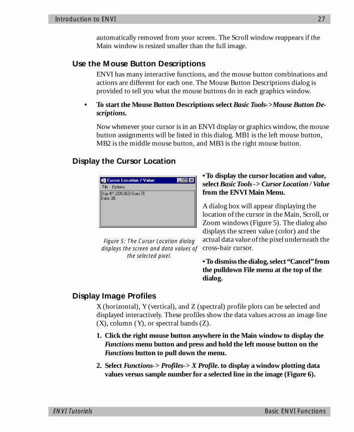
Introduction to ENVI 27
automatically removed from your screen. The Scroll window reappears if the Main window is resized smaller than the full image.
Use the Mouse Button DescriptionsENVI has many interactive functions, and the mouse button combinations and actions are different for each one. The Mouse Button Descriptions dialog is provided to tell you what the mouse buttons do in each graphics window.
• To start the Mouse Button Descriptions select Basic Tools->Mouse Button De-scriptions.
Now whenever your cursor is in an ENVI display or graphics window, the mouse button assignments will be listed in this dialog. MB1 is the left mouse button, MB2 is the middle mouse button, and MB3 is the right mouse button.
Display the Cursor Location
•To display the cursor location and value, select Basic Tools -> Cursor Location / Value from the ENVI Main Menu.
A dialog box will appear displaying the location of the cursor in the Main, Scroll, or Zoom windows (Figure 5). The dialog also displays the screen value (color) and the actual data value of the pixel underneath the cross-hair cursor.
•To dismiss the dialog, select “Cancel” from the pulldown File menu at the top of the dialog.
Display Image ProfilesX (horizontal), Y (vertical), and Z (spectral) profile plots can be selected and displayed interactively. These profiles show the data values across an image line (X), column (Y), or spectral bands (Z).
1. Click the right mouse button anywhere in the Main window to display the Functions menu button and press and hold the left mouse button on the Functions button to pull down the menu.
2. Select Functions-> Profiles-> X Profile. to display a window plotting data values versus sample number for a selected line in the image (Figure 6).
Figure 5: The Cursor Location dialog displays the screen and data values of
the selected pixel.
ENVI Tutorials Basic ENVI Functions
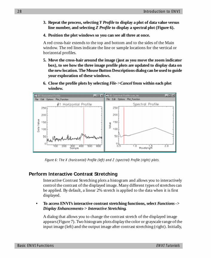
28 Introduction to ENVI
3. Repeat the process, selecting Y Profile to display a plot of data value versus line number, and selecting Z Profile to display a spectral plot (Figure 6).
4. Position the plot windows so you can see all three at once.
A red cross-hair extends to the top and bottom and to the sides of the Main window. The red lines indicate the line or sample locations for the vertical or horizontal profiles.
5. Move the cross-hair around the image (just as you move the zoom indicator box), to see how the three image profile plots are updated to display data on the new location. The Mouse Button Descriptions dialog can be used to guide your exploration of these windows.
6. Close the profile plots by selecting File->Cancel from within each plot window.
Perform Interactive Contrast StretchingInteractive Contrast Stretching plots a histogram and allows you to interactively control the contrast of the displayed image. Many different types of stretches can be applied. By default, a linear 2% stretch is applied to the data when it is first displayed.
• To access ENVI’s interactive contrast stretching functions, select Functions -> Display Enhancements-> Interactive Stretching.
A dialog that allows you to change the contrast stretch of the displayed image appears (Figure 7). Two histogram plots display the color or grayscale range of the input image (left) and the output image after contrast stretching (right). Initially,
Figure 6: The X (horizontal) Profile (left) and Z (spectral) Profile (right) plots.
Basic ENVI Functions ENVI Tutorials
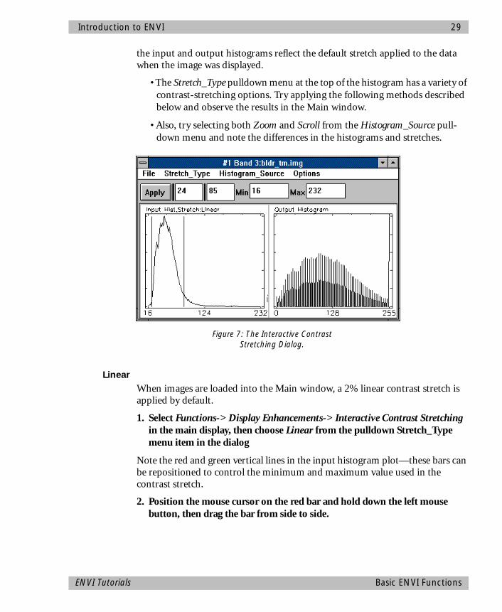
Introduction to ENVI 29
the input and output histograms reflect the default stretch applied to the data when the image was displayed.
• The Stretch_Type pulldown menu at the top of the histogram has a variety of contrast-stretching options. Try applying the following methods described below and observe the results in the Main window.
• Also, try selecting both Zoom and Scroll from the Histogram_Source pull-down menu and note the differences in the histograms and stretches.
LinearWhen images are loaded into the Main window, a 2% linear contrast stretch is applied by default.
1. Select Functions-> Display Enhancements-> Interactive Contrast Stretching in the main display, then choose Linear from the pulldown Stretch_Type menu item in the dialog
Note the red and green vertical lines in the input histogram plot—these bars can be repositioned to control the minimum and maximum value used in the contrast stretch.
2. Position the mouse cursor on the red bar and hold down the left mouse button, then drag the bar from side to side.
Figure 7: The Interactive Contrast Stretching Dialog.
ENVI Tutorials Basic ENVI Functions

30 Introduction to ENVI
Numbers above the plot display the current data value, the number of pixels and the percentage of pixels that have that value, and the cumulative percentage of pixels with values less than or equal to the current value.
3. Try positioning the red bar so that approximately 5% of the pixels are selected, and the green bar so that approximately 95% of the pixels are selected.
4. Click “Apply” to apply the stretch and observe the results.
• You can also position the bars by entering minimum and maximum values in the fields next to the “Apply” button at the top of the dialog. You can enter either data values or percentages.
5. Enter “4%” in the left box and “96%” in the right box (press Enter after typing each value) and click “Apply”.
The red and green bars will be adjusted and the two text entries updated to display the data values at 4% and 96%, respectively.
Equalize1. Select Stretch_Type->Equalization and note the change in the “Output
Histogram” display.
2. Click “Apply” to apply the stretch shown in the output histogram plot to the image in the Main window.
Gaussian1. Select Stretch_Type -> Gaussian.
2. Set the Standard Deviation by selecting Options -> Set Gaussian Stdv.
3. Apply the stretch and note the change in the Main window.
4. Click “Cancel” to close the contrast stretching dialog.
Display Interactive Scatter PlotsYou can plot the data values of two selected image bands versus each other in a scatter plot to graphically display the overlapping values.
1. Select Functions->Interactive Analysis->2D Scatter Plots in the Main window.
A dialog will appear that lets you choose two image bands to compare.
2. Select one band for the X axis and another band for the Y axis and click “OK.”
It may take a few seconds for ENVI to extract and tabulate the data values.
Basic ENVI Functions ENVI Tutorials
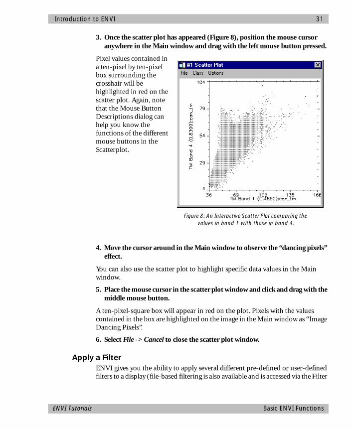
Introduction to ENVI 31
3. Once the scatter plot has appeared (Figure 8), position the mouse cursor anywhere in the Main window and drag with the left mouse button pressed.
Pixel values contained in a ten-pixel by ten-pixel box surrounding the crosshair will be highlighted in red on the scatter plot. Again, note that the Mouse Button Descriptions dialog can help you know the functions of the different mouse buttons in the Scatterplot.
4. Move the cursor around in the Main window to observe the “dancing pixels” effect.
You can also use the scatter plot to highlight specific data values in the Main window.
5. Place the mouse cursor in the scatter plot window and click and drag with the middle mouse button.
A ten-pixel-square box will appear in red on the plot. Pixels with the values contained in the box are highlighted on the image in the Main window as “Image Dancing Pixels”.
6. Select File -> Cancel to close the scatter plot window.
Apply a FilterENVI gives you the ability to apply several different pre-defined or user-defined filters to a display (file-based filtering is also available and is accessed via the Filter
Figure 8: An Interactive Scatter Plot comparing the values in band 1 with those in band 4.
ENVI Tutorials Basic ENVI Functions
32 Introduction to ENVI
menu on the ENVI main menu). The following example shows you how to apply a pre-defined filter to the image in the Main display window.
Choose a Filter 1. Select Functions->Display Enhancements->Filter and choose the desired
filter type from the pulldown filter menu to apply a filter to the displayed image.
2. Try the different sharpening, smoothing, median, and edge detection filters on the displayed image.
Display A Second Image and Apply Filter1. Click “New” in the Available Bands List dialog to create a second display
group, select an image band, and click “Load Band” to load the image into the second display. Choose Functions->Display Enhancements->Filter and select a filter different from that applied to image #1 from the pulldown filter menu.
Link Two DisplaysLink the two displays together to compare the filter results. When you link two displays, any action you perform on one display (scrolling, zooming, etc.) is echoed in the linked display. To link the two displays you have on screen now:
1. Select Functions ->Link- >Link Displays from one of the display windows.
2. Click “OK” in the Link Displays dialog.
3. Now try scrolling or zooming in one display group and observe as your changes are mirrored in the second display.
Dynamic OverlaysENVI’s Multiple Dynamic Overlay feature allows you to dynamically superimpose parts of one or more linked images onto the other image. Dynamic overlays are turned on automatically when you link two displays.
• To use the overlay, position the mouse cursor anywhere in either Main window and hold down and drag with the left mouse button.
A small portion of the linked image will be superimposed on the current image window. The overlay will appear in either the Main window or the Zoom window.
• To change the size of the overlay area, hold down the middle mouse button and drag the overlay area until it is the desired size.
Basic ENVI Functions ENVI Tutorials
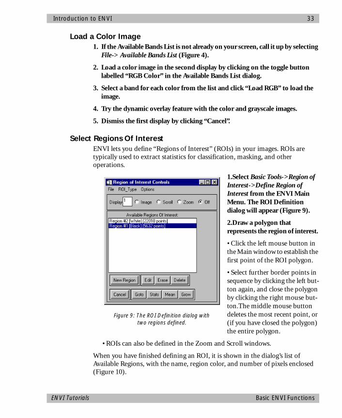
Introduction to ENVI 33
Load a Color Image1. If the Available Bands List is not already on your screen, call it up by selecting
File-> Available Bands List (Figure 4).
2. Load a color image in the second display by clicking on the toggle button labelled “RGB Color” in the Available Bands List dialog.
3. Select a band for each color from the list and click “Load RGB” to load the image.
4. Try the dynamic overlay feature with the color and grayscale images.
5. Dismiss the first display by clicking “Cancel”.
Select Regions Of InterestENVI lets you define “Regions of Interest” (ROIs) in your images. ROIs are typically used to extract statistics for classification, masking, and other operations.
1.Select Basic Tools->Region of Interest->Define Region of Interest from the ENVI Main Menu. The ROI Definition dialog will appear (Figure 9).
2.Draw a polygon that represents the region of interest.
• Click the left mouse button in the Main window to establish the first point of the ROI polygon.
• Select further border points in sequence by clicking the left but-ton again, and close the polygon by clicking the right mouse but-ton.The middle mouse button deletes the most recent point, or (if you have closed the polygon) the entire polygon.
• ROIs can also be defined in the Zoom and Scroll windows.
When you have finished defining an ROI, it is shown in the dialog’s list of Available Regions, with the name, region color, and number of pixels enclosed (Figure 10).
Figure 9: The ROI Definition dialog with two regions defined.
ENVI Tutorials Basic ENVI Functions
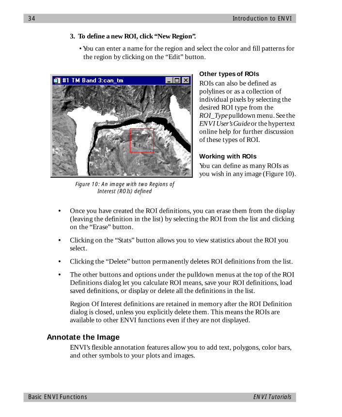
34 Introduction to ENVI
3. To define a new ROI, click “New Region”.
• You can enter a name for the region and select the color and fill patterns for the region by clicking on the “Edit” button.
Other types of ROIsROIs can also be defined as polylines or as a collection of individual pixels by selecting the desired ROI type from the ROI_Type pulldown menu. See the ENVI User’s Guide or the hypertext online help for further discussion of these types of ROI.
Working with ROIsYou can define as many ROIs as you wish in any image (Figure 10).
• Once you have created the ROI definitions, you can erase them from the display (leaving the definition in the list) by selecting the ROI from the list and clicking on the “Erase” button.
• Clicking on the “Stats” button allows you to view statistics about the ROI you select.
• Clicking the “Delete” button permanently deletes ROI definitions from the list.
• The other buttons and options under the pulldown menus at the top of the ROI Definitions dialog let you calculate ROI means, save your ROI definitions, load saved definitions, or display or delete all the definitions in the list.
Region Of Interest definitions are retained in memory after the ROI Definition dialog is closed, unless you explicitly delete them. This means the ROIs are available to other ENVI functions even if they are not displayed.
Annotate the ImageENVI’s flexible annotation features allow you to add text, polygons, color bars, and other symbols to your plots and images.
Figure 10: An image with two Regions of Interest (ROIs) defined
Basic ENVI Functions ENVI Tutorials
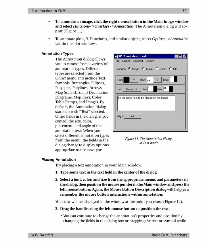
Introduction to ENVI 35
• To annotate an image, click the right mouse button in the Main Image window and select Functions- >Overlays ->Annotation. The Annotation dialog will ap-pear (Figure 11).
• To annotate plots, 3-D surfaces, and similar objects, select Options ->Annotation within the plot windows.
Annotation TypesThe Annotation dialog allows you to choose from a variety of annotation types. Different types are selected from the Object menu and include Text, Symbols, Rectangles, Ellipses, Polygons, Polylines, Arrows, Map Scale Bars and Declination Diagrams, Map Keys, Color Table Ramps, and Images. By default, the Annotation dialog starts up with “Text” selected. Other fields in the dialog let you control the size, color, placement, and angle of the annotation text. When you select different annotation types from the menu, the fields in the dialog change to display options appropriate to the new type.
Placing AnnotationTry placing a text annotation in your Main window:
1. Type some text in the text field in the center of the dialog.
2. Select a font, color, and size from the appropriate menus and parameters in the dialog, then position the mouse pointer in the Main window and press the left mouse button. Again, the Mouse Button Description dialog will help you remember the mouse button interactions within annotation.
Your text will be displayed in the window at the point you chose (Figure 12).
3. Drag the handle using the left mouse button to position the text.
• You can continue to change the annotation’s properties and position by changing the fields in the dialog box or dragging the text or symbol while
Figure 11: The Annotation dialog, in Text mode.
ENVI Tutorials Basic ENVI Functions

36 Introduction to ENVI
holding down the left mouse button.
4. When you are satisfied with the annotation, press the right mouse button to fix the annotation in position.
Saving and Restoring Annotation
• You can save your image annotation by selecting File- >Save Annotation in the Annotation dialog.
Note If you do not save your annotation in a file, it will be lost when you close the Annotation dialog (you will be prompted to save the annotation if you close without first saving).
• You can also restore saved annotation files by selecting File ->Restore Annotation in the dialog.
Editing Previously Placed AnnotationTo edit an annotation element that has already been “fixed” on the image:
1. Select Object- >Selection/Edit in the Annotation dialog.
2. Draw a box around the annotation you wish to edit by clicking and dragging with the left mouse button.
3. When the handle reappears, move and configure the item just as you would a new annotation.
Figure 12: An annotated image
Basic ENVI Functions ENVI Tutorials
Introduction to ENVI 37
Suspending the Annotation Function Temporarily
• To suspend annotation operations and return to normal ENVI functionality temporarily, select the “Off” toggle button at the top of the Annotation dialog.
This allows you to use the scroll and zoom features in your display without losing your annotations.
• To return to the annotation function, select the toggle button for the window you are annotating.
Leave your annotation on the Main window image as you complete this tutorial.
Add Grid LinesTry adding a grid (Figure 13to your image:
1. To overlay grid lines on your image, select Functions->Overlays->Grid Lines in the Main display window.
• You can adjust the grid lines by setting the line thickness and color and the grid spacing using the Options pulldown menu.
An image border is automatically added when you overlay grid lines.
2. When you have added a satisfactory grid, click “Apply” in the Grid Line Parameters dialog.
Save and Output an ImageENVI gives you several options for saving and outputting your filtered, annotated, gridded images. You can save your work in ENVI’s image file format (Figure 20), or in several popular graphics formats (including Postscript) for printing or importing into other software packages.
Saving your Image in ENVI Image FormatTo save your work in ENVI’s native format (as an RGB file):
1. Select Functions->Output Display ->Image File in the Main window.
The Output Display to Image Parameters dialog will appear.
2. Select 24-Bit color or 8-Bit grayscale output, graphics options (including annotation and gridlines), and borders.
If you have left your annotated and gridded color image on the display, both the annotation and grid lines will be automatically listed in the graphics options.
You can also select other annotation files to be “burned in” to the output image.
ENVI Tutorials Basic ENVI Functions
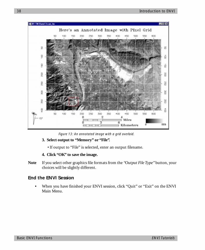
38 Introduction to ENVI
3. Select output to “Memory” or “File”.
• If output to “File” is selected, enter an output filename.
4. Click “OK” to save the image.
Note If you select other graphics file formats from the “Output File Type” button, your choices will be slightly different.
End the ENVI Session
• When you have finished your ENVI session, click “Quit” or “Exit” on the ENVI Main Menu.
Figure 13: An annotated image with a grid overlaid.
Basic ENVI Functions ENVI Tutorials
ENVI Tutorial #2
Multispectral Classification
The following topics are covered in this tutorial:
Overview of This Tutorial ........................................................................................40Examine Landsat TM Color Images .........................................................................41Unsupervised Classification .....................................................................................44Supervised Classification .........................................................................................45Post Classification Processing ..................................................................................52Classes to Vector Layers ..........................................................................................56Classification Keys Using Annotation .......................................................................56
39
40 Multispectral Classification
Overview of This TutorialThis tutorial leads you through a typical multispectral classification procedure using Landsat TM data from Canon City, Colorado. Results of both unsupervised and supervised classifications are examined and post classification processing including clump, sieve, combine classes, and accuracy assessment are discussed. It is assumed that you are already generally familiar with multispectral classification techniques.
Files Used in This TutorialYou must have the ENVI TUTORIALS & DATA CD-ROM mounted on your system to access the files usedby this tutorial, or copy the files to your disk.
The files used in this tutorial are contained in theCAN_TM subdirectory of the ENVIDATA directory onthe ENVI TUTORIALS & DATA CD-ROM.
Required FilesThe files listed below are required to run this exercise.
CAN_TMR.IMG Boulder Colorado TM Re-flectance
CAN_TMR.HDR ENVI Header for Above
CAN_KM.IMG KMEANS Classification
CAN_KM.HDR ENVI Header for Above
CAN_ISO.IMG ISODATA Classification
CAN_ISO.HDR ENVI Header for Above
CLASSES.ROI Regions of Interest (ROI) for Supervised Classification
CAN_PCLS.IMG Paralleleliped Classification
CAN_PCLS.HDR ENVI Header for Above
CAN_BIN.IMG Binary Encoding Result
CAN_BIN.HDR ENVI Header for Above
CAN_SAM.IMG SAM Classification Result
CAN_SAM.HDR ENVI Header for Above
CAN_RUL.IMG Rule image for SAM classification
CAN_RUL.HDR ENVI Header for Above
CAN_SV.IMG Sieved Image
Topics Covered in This TutorialExamine Landsat TM Color Images• Open and Display TM Data• Review Image Colors• Cursor Location/Value• Examine Spectral Plots
Unsupervised Classification• K-Means• Isodata
Supervised Classification• Select Training Sets Using ROIs• Classical Supervised
Multispectral Classification• Spectral Classification Methods• Endmember Collection• Binary Encoding• Spectral Angle Mapper• Rule Images
Post Classification Processing• Class Statistics• Confusion Matrix• Clump and Sieve• Combine Classes• Edit Class Colors• Overlay Classes• Classes to Vector Overlays
Classification Keys using Annotation
Overview of This Tutorial ENVI Tutorials
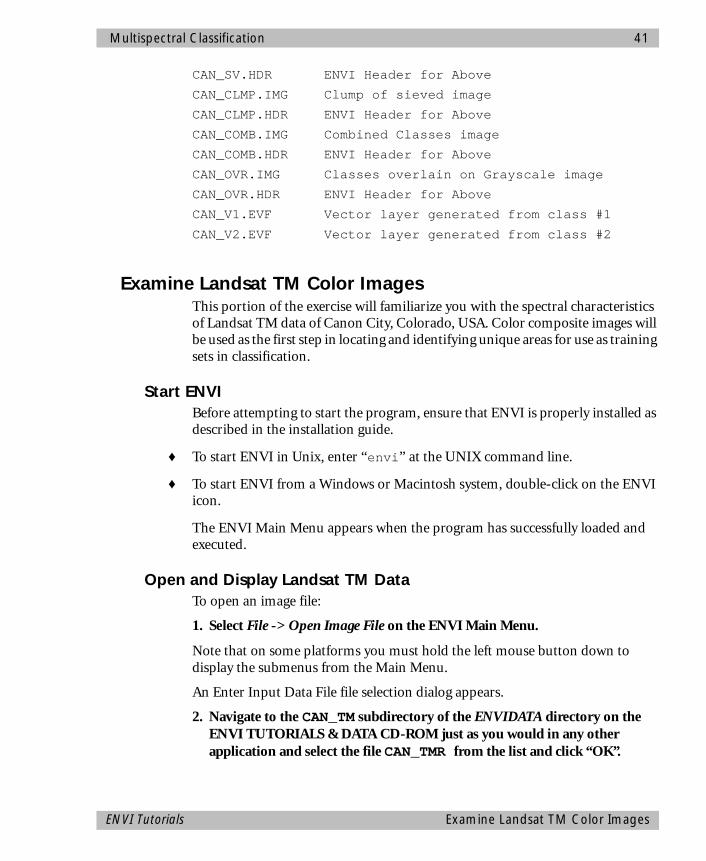
Multispectral Classification 41
CAN_SV.HDR ENVI Header for Above
CAN_CLMP.IMG Clump of sieved image
CAN_CLMP.HDR ENVI Header for Above
CAN_COMB.IMG Combined Classes image
CAN_COMB.HDR ENVI Header for Above
CAN_OVR.IMG Classes overlain on Grayscale image
CAN_OVR.HDR ENVI Header for Above
CAN_V1.EVF Vector layer generated from class #1
CAN_V2.EVF Vector layer generated from class #2
Examine Landsat TM Color ImagesThis portion of the exercise will familiarize you with the spectral characteristics of Landsat TM data of Canon City, Colorado, USA. Color composite images will be used as the first step in locating and identifying unique areas for use as training sets in classification.
Start ENVIBefore attempting to start the program, ensure that ENVI is properly installed as described in the installation guide.
♦ To start ENVI in Unix, enter “envi” at the UNIX command line.
♦ To start ENVI from a Windows or Macintosh system, double-click on the ENVI icon.
The ENVI Main Menu appears when the program has successfully loaded and executed.
Open and Display Landsat TM DataTo open an image file:
1. Select File -> Open Image File on the ENVI Main Menu.
Note that on some platforms you must hold the left mouse button down to display the submenus from the Main Menu.
An Enter Input Data File file selection dialog appears.
2. Navigate to the CAN_TM subdirectory of the ENVIDATA directory on the ENVI TUTORIALS & DATA CD-ROM just as you would in any other application and select the file CAN_TMR from the list and click “OK”.
ENVI Tutorials Examine Landsat TM Color Images
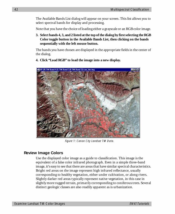
42 Multispectral Classification
The Available Bands List dialog will appear on your screen. This list allows you to select spectral bands for display and processing.
Note that you have the choice of loading either a grayscale or an RGB color image.
3. Select bands 4, 3, and 2 listed at the top of the dialog by first selecting the RGB Color toggle button in the Available Bands List, then clicking on the bands sequentially with the left mouse button.
The bands you have chosen are displayed in the appropriate fields in the center of the dialog.
4. Click “Load RGB” to load the image into a new display.
Review Image ColorsUse the displayed color image as a guide to classification. This image is the equivalent of a false color infrared photograph. Even in a simple three-band image, it’s easy to see that there are areas that have similar spectral characteristics. Bright red areas on the image represent high infrared reflectance, usually corresponding to healthy vegetation, either under cultivation, or along rivers. Slightly darker red areas typically represent native vegetation, in this case in slightly more rugged terrain, primarily corresponding to coniferous trees. Several distinct geologic classes are also readily apparent as is urbanization.
Figure 1: Canon City Landsat TM Data.
Examine Landsat TM Color Images ENVI Tutorials
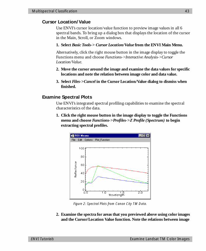
Multispectral Classification 43
Cursor Location/Value
Use ENVI’s cursor location/value function to preview image values in all 6 spectral bands. To bring up a dialog box that displays the location of the cursor in the Main, Scroll, or Zoom windows.
1. Select Basic Tools-> Cursor Location/Value from the ENVI Main Menu.
Alternatively, click the right mouse button in the image display to toggle the Functions menu and choose Functions->Interactive Analysis->Cursor Location/Value.
2. Move the cursor around the image and examine the data values for specific locations and note the relation between image color and data value.
3. Select Files->Cancel in the Cursor Location/Value dialog to dismiss when finished.
Examine Spectral PlotsUse ENVI’s integrated spectral profiling capabilities to examine the spectral characteristics of the data.
1. Click the right mouse button in the image display to toggle the Functions menu and choose Functions->Profiles->Z Profile (Spectrum) to begin extracting spectral profiles.
2. Examine the spectra for areas that you previewed above using color images and the Cursor/Location Value function. Note the relations between image
Figure 2: Spectral Plots from Canon City TM Data.
ENVI Tutorials Examine Landsat TM Color Images

44 Multispectral Classification
color and spectral shape. Pay attention to the location of the image bands in the spectral profile, marked by the red, green, and blue bars in the plot.
Unsupervised ClassificationStart ENVI’s unsupervised classification routines by choosing Classification->Unsupervised->Method, where Method is either K-Means or Isodata, or review the precalculated results of classifying the image in the CAN_TM directory.
K-MeansUnsupervised classification uses statistical techniques to group n-dimensional data into their natural spectral classes. The K-Means unsupervised classifier uses a cluster analysis approach which requires the analyst to select the number of clusters to be located in the data, arbitrarily locates this number of cluster centers, then iteratively repositions them until optimal spectral separability is achieved.
Choose K-Means as the method, use all of the default values and click on OK, or review the results contained in CAN_KM.IMG.
1. Open the file CAN_KM.IMG, click on the grayscale radio button in the Available Bands List, click on the band name at the top of the List, click New, and then Load Band.
2. Click the right mouse button in the Main Image Display window to toggle the Functions menu then select Functions->Link->Link Displays and click OK in the dialog to link the images.
3. Compare the K-MEANS classification result to the color composite image by clicking and dragging using the left mouse button to move the dynamic overlay around the image.
4. When finished, select Functions->Link->Unlink Displays to remove the link and dynamic overlay.
If desired, experiment with different numbers of classes, Change Thresholds, Standard Deviations, and Maximum Distance Error values to determine their effect on the classification.
IsodataIsoData unsupervised classification calculates class means evenly distributed in the data space and then iteratively clusters the remaining pixels using minimum distance techniques. Each iteration recalculates means and reclassifies pixels with respect to the new means. This process continues until the number of pixels in
Unsupervised Classification ENVI Tutorials

Multispectral Classification 45
each class changes by less than the selected pixel change threshold or the maximum number of iterations is reached.
Choose ISODATA as the method, use all of the default values and click on OK, or review the results contained in CAN_ISO.IMG.
1. Open the file CAN_ISO.IMG, click on the grayscale radio button in the Available Bands List, click on the band name at the top of the List, click New, and then Load Band.
2. Click the right mouse button in the Main Image Display window to toggle the Functions menu then select Functions->Link->Link Displays. Click OK to link this image to the color composite image and the KMEANS result.
3. Compare the ISODATA classification result to the color composite image by clicking and dragging using the left mouse button to move the dynamic overlay around the image. Toggle the dynamic overlay of the third image by holding the left mouse button down and simultaneously clicking on the middle mouse button. Compare the ISODATA and K-MEANS classifications.
4. Click the right mouse button in each of the classified images to toggle the Functions menu and click Cancel to dismiss the two image displays.
If desired, experiment with different numbers of classes, Change Thresholds, Standard Deviations, Maximum Distance Error, and class pixel characteristic values to determine their effect on the classification.
Supervised ClassificationSupervised classification requires that the user select training areas for use as the basis for classification. Various comparison methods are then used to determine if a specific pixel qualifies as a class member. ENVI provides a broad range of different classification methods, including Parallelepiped, Maximum Likelihood, Minimum Distance, Mahalanobis Distance, Binary Encoding, and Spectral Angle Mapper. Examine the processing results below, or use the default classification parameters for each of these classification methods to generate your own classes and compare results.
To perform your own classifications use Classification->Supervised->Method, where Method is one of ENVI’s supervised classification methods. Use one of the two methods below for selecting training areas (Regions of Interest).
Select Training Sets Using Regions of Interest (ROI)As described in ENVI Tutorial #1 and summarized here, ENVI lets you easily define “Regions of Interest” (ROIs) typically used to extract statistics for
ENVI Tutorials Supervised Classification

46 Multispectral Classification
classification, masking, and other operations. For the purposes of this exercise, you can either use predefined ROIs, or create your own.
Restore Predefined ROIs1. Use preselected Regions of Interest by starting the Region of Interest Controls
dialog by choosing Basic Tools->Region of Interest->Define Region of Interest, then choosing File->Restore ROIs and choosing CLASSES.ROI as the input file.
Create Your Own ROIs1. Select Basic Tools->Region of Interest->Define Region of Interest from the
ENVI Main Menu. The ROI Definition dialog will appear.
2. Draw a polygon that represents the region of interest.
• Click the left mouse button in the Main window to establish the first point of the ROI polygon.
• Select further border points in sequence by clicking the left button again, and close the polygon by clicking the right mouse button.The middle mouse but-ton deletes the most recent point, or (if you have closed the polygon) the entire polygon.
• ROIs can also be defined in the Zoom and Scroll windows by choosing the appropriate radio button at the top of the ROI Controls dialog.
When you have finished defining an ROI, it is shown in the dialog’s list of Available Regions, with the name, region color, and number of pixels enclosed, and is available to all of ENVI’s classification procedures.
3. To define a new ROI, click “New Region”.
• You can enter a name for the region and select the color and fill patterns for the region by clicking on the “Edit” button. Define the new ROI as described above.
Classical Supervised Multispectral ClassificationThe following methods are described in most remote sensing textbooks and are commonly available in today’s image processing software systems.
ParallelepipedParallelepiped classification uses a simple decision rule to classify multispectral data. The decision boundaries form an n-dimensional parallelepiped in the image data space. The dimensions of the parallelepiped are defined based upon a standard deviation threshold from the mean of each selected class.
Supervised Classification ENVI Tutorials
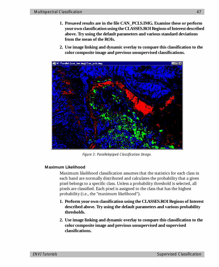
Multispectral Classification 47
1. Presaved results are in the file CAN_PCLS.IMG. Examine these or perform your own classification using the CLASSES.ROI Regions of Interest described above. Try using the default parameters and various standard deviations from the mean of the ROIs.
2. Use image linking and dynamic overlay to compare this classification to the color composite image and previous unsupervised classifications.
Maximum LikelihoodMaximum likelihood classification assumes that the statistics for each class in each band are normally distributed and calculates the probability that a given pixel belongs to a specific class. Unless a probability threshold is selected, all pixels are classified. Each pixel is assigned to the class that has the highest probability (i.e., the "maximum likelihood").
1. Perform your own classification using the CLASSES.ROI Regions of Interest described above. Try using the default parameters and various probability thresholds.
2. Use image linking and dynamic overlay to compare this classification to the color composite image and previous unsupervised and supervised classifications.
Figure 3: Parallelepiped Classification Image.
ENVI Tutorials Supervised Classification

48 Multispectral Classification
Minimum DistanceThe minimum distance classification uses the mean vectors of each ROI and calculates the Euclidean distance from each unknown pixel to the mean vector for each class. All pixels are classified to the closest ROI class unless the user specifies standard deviation or distance thresholds, in which case some pixels may be unclassified if they do not meet the selected criteria.
1. Perform your own classification using the CLASSES.ROI Regions of Interest described above. Try using the default parameters and various standard deviations and maximum distance errors.
2. Use image linking and dynamic overlay to compare this classification to the color composite image and previous unsupervised and supervised classifications.
Mahalanobis DistanceThe Mahalanobis Distance classification is a direction sensitive distance classifier that uses statistics for each class. It is similar to the Maximum Likelihood classification but assumes all class covariances are equal and therefore is a faster method. All pixels are classified to the closest ROI class unless the user specifies a distance threshold, in which case some pixels may be unclassified if they do not meet the threshold.
1. Perform your own classification using the CLASSES.ROI Regions of Interest described above. Try using the default parameters and various maximum distance errors.
2. Use image linking and dynamic overlay to compare this classification to the color composite image and previous unsupervised and supervised classifications.
“Spectral” Classification MethodsThe following methods are described in the ENVI Users’s guide. These were developed specifically for use on Hyperspectral data, but provide an alternative method for classifying multispectral data, often with improved results that can easily be compared to spectral properties of materials. They typically are used from the Endmember Collection dialog using image or library spectra, however, they can also be started from the classification menu, Classification->Supervised->Method.
The Endmember Collection DialogThe endmember collection dialog is a standardized means of collecting spectra for supervised classification from ASCII Files, Regions of Interest, Spectral
Supervised Classification ENVI Tutorials
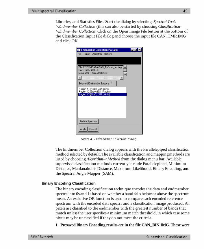
Multispectral Classification 49
Libraries, and Statistics Files. Start the dialog by selecting, Spectral Tools->Endmember Collection (this can also be started by choosing Classification->Endmember Collection. Click on the Open Image File button at the bottom of the Classification Input File dialog and choose the input file CAN_TMR.IMG and click OK.
The Endmember Collection dialog appears with the Parallelepiped classification method selected by default. The available classification and mapping methods are listed by choosing Algorithm->Method from the dialog menu bar. Available supervised classification methods currently include Parallelepiped, Minimum Distance, Manlanahobis Distance, Maximum Likelihood, Binary Encoding, and the Spectral Angle Mapper (SAM).
Binary Encoding ClassificationThe binary encoding classification technique encodes the data and endmember spectra into 0s and 1s based on whether a band falls below or above the spectrum mean. An exclusive OR function is used to compare each encoded reference spectrum with the encoded data spectra and a classification image produced. All pixels are classified to the endmember with the greatest number of bands that match unless the user specifies a minimum match threshold, in which case some pixels may be unclassified if they do not meet the criteria.
1. Presaved Binary Encoding results are in the file CAN_BIN.IMG. These were
Figure 4: Endmember Collection dialog.
ENVI Tutorials Supervised Classification

50 Multispectral Classification
created using a minimum encoding threshold of 75%. Examine these or perform your own classification using the CLASSES.ROI Regions of Interest described above. To do your own classification, elect Algorithm->Binary Encoding from the menu bar. Use the predefined Regions of Interest in the file CLASSES.ROI. Select Import->From ROI from input file, click on Select All, and click OK. You can view the spectral plots for he ROIs by choosing Options->Plot Endmembers.
2. Click on the arrow toggle button next to the text “Output Rule Images” in the Binary Encoding Parameters dialog to and click OK at the bottom of the dialog to start the classification.
3. Use image linking and dynamic overlays to compare this classification to the color composite image and previous unsupervised and supervised classifications.
Spectral Angle Mapper ClassificationThe Spectral Angle Mapper (SAM) is a physically-based spectral classification that uses the n-dimensional angle to match pixels to reference spectra. The algorithm determines the spectral similarity between two spectra by calculating the angle between the spectra, treating them as vectors in a space with dimensionality equal to the number of bands.
1. Presaved SAM Classification results are in the file CAN_SAM.IMG. Examine these or perform your own classification using the CLASSES.ROI Regions of Interest described above, which will be listed in the Endmember Collection dialog. To do your own classification, select Algorithm->Spectral Angle Mapper from the menu bar. Click Apply to start the classification.
2. If performing your own classification, enter an output filename for the SAM classification image in the Endmember Collection dialog. Also enter the filename CAN_RUL.IMG as the rule output image name and click OK at the bottom of the dialog to start the classification.
Use image linking and dynamic overlays to compare this classification to the color composite image and previous unsupervised and supervised classifications.
Rule ImagesENVI creates images that show the pixel values used to create the classified image. These optional images allow users to evaluate classification results and to reclassify if desired based on thresholds. These are grayscale images; one for each ROI or endmember spectrum used in the classification.
Supervised Classification ENVI Tutorials
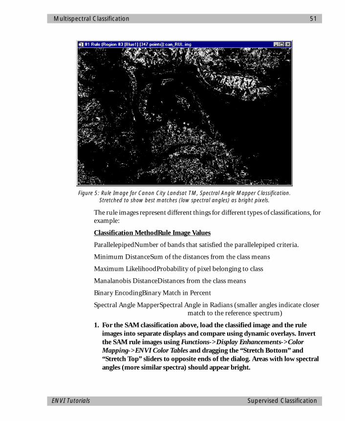
Multispectral Classification 51
The rule images represent different things for different types of classifications, for example:
Classification MethodRule Image Values
ParallelepipedNumber of bands that satisfied the parallelepiped criteria.
Minimum DistanceSum of the distances from the class means
Maximum LikelihoodProbability of pixel belonging to class
Manalanobis DistanceDistances from the class means
Binary EncodingBinary Match in Percent
Spectral Angle MapperSpectral Angle in Radians (smaller angles indicate closer match to the reference spectrum)
1. For the SAM classification above, load the classified image and the rule images into separate displays and compare using dynamic overlays. Invert the SAM rule images using Functions->Display Enhancements->Color Mapping->ENVI Color Tables and dragging the “Stretch Bottom” and “Stretch Top” sliders to opposite ends of the dialog. Areas with low spectral angles (more similar spectra) should appear bright.
Figure 5: Rule Image for Canon City Landsat TM, Spectral Angle Mapper Classification. Stretched to show best matches (low spectral angles) as bright pixels.
ENVI Tutorials Supervised Classification
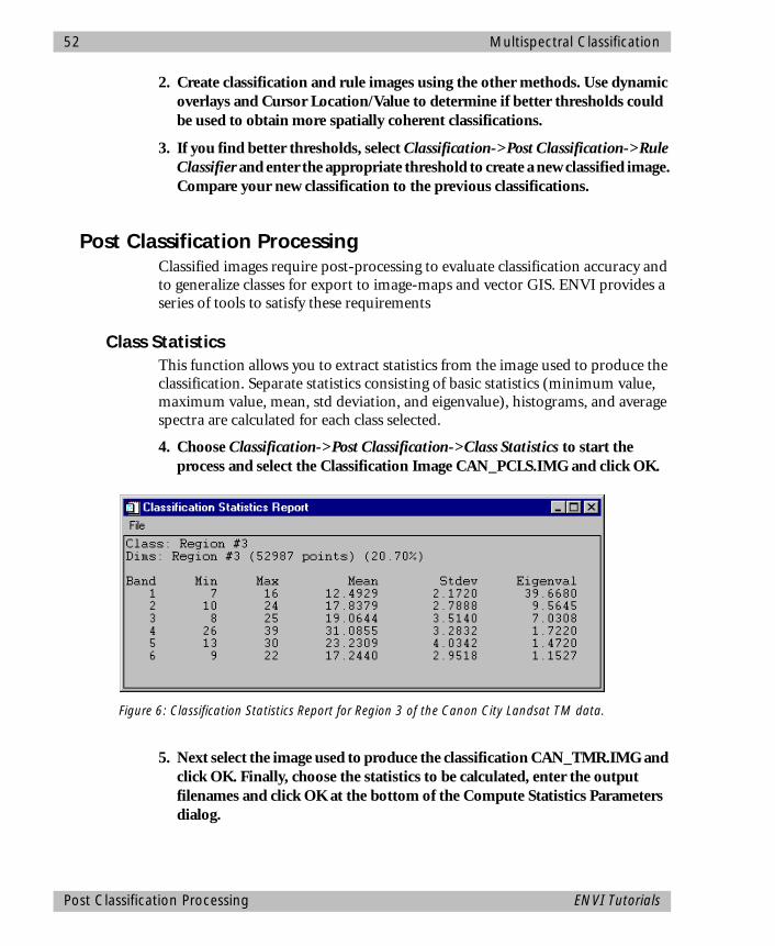
52 Multispectral Classification
2. Create classification and rule images using the other methods. Use dynamic overlays and Cursor Location/Value to determine if better thresholds could be used to obtain more spatially coherent classifications.
3. If you find better thresholds, select Classification->Post Classification->Rule Classifier and enter the appropriate threshold to create a new classified image. Compare your new classification to the previous classifications.
Post Classification ProcessingClassified images require post-processing to evaluate classification accuracy and to generalize classes for export to image-maps and vector GIS. ENVI provides a series of tools to satisfy these requirements
Class StatisticsThis function allows you to extract statistics from the image used to produce the classification. Separate statistics consisting of basic statistics (minimum value, maximum value, mean, std deviation, and eigenvalue), histograms, and average spectra are calculated for each class selected.
4. Choose Classification->Post Classification->Class Statistics to start the process and select the Classification Image CAN_PCLS.IMG and click OK.
5. Next select the image used to produce the classification CAN_TMR.IMG and click OK. Finally, choose the statistics to be calculated, enter the output filenames and click OK at the bottom of the Compute Statistics Parameters dialog.
Figure 6: Classification Statistics Report for Region 3 of the Canon City Landsat TM data.
Post Classification Processing ENVI Tutorials
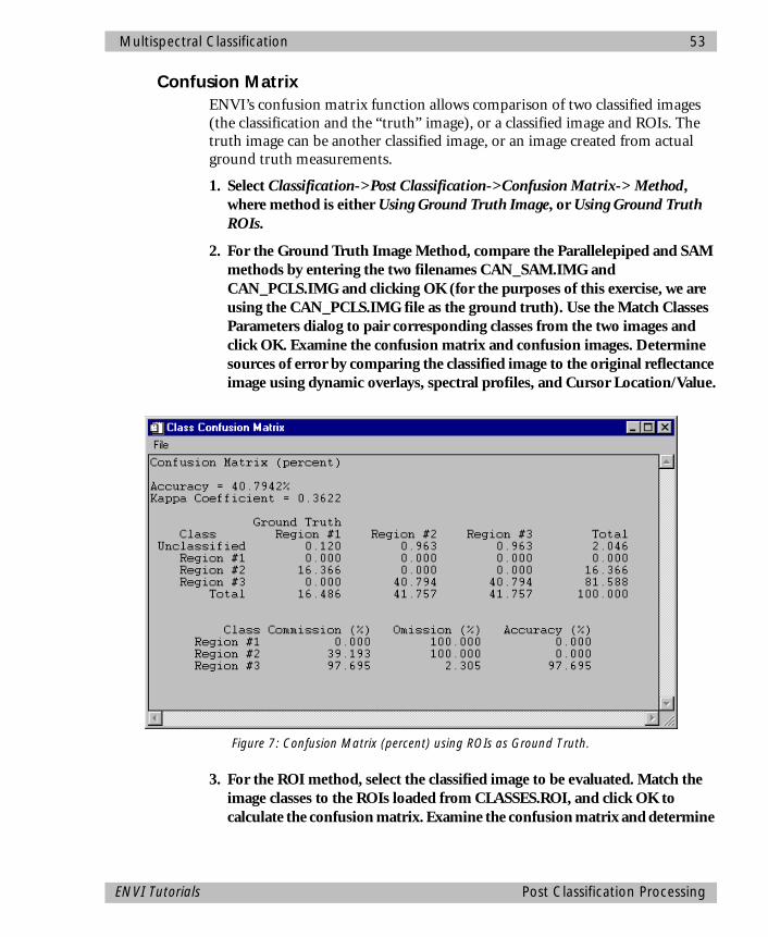
Multispectral Classification 53
Confusion MatrixENVI’s confusion matrix function allows comparison of two classified images (the classification and the “truth” image), or a classified image and ROIs. The truth image can be another classified image, or an image created from actual ground truth measurements.
1. Select Classification->Post Classification->Confusion Matrix-> Method, where method is either Using Ground Truth Image, or Using Ground Truth ROIs.
2. For the Ground Truth Image Method, compare the Parallelepiped and SAM methods by entering the two filenames CAN_SAM.IMG and CAN_PCLS.IMG and clicking OK (for the purposes of this exercise, we are using the CAN_PCLS.IMG file as the ground truth). Use the Match Classes Parameters dialog to pair corresponding classes from the two images and click OK. Examine the confusion matrix and confusion images. Determine sources of error by comparing the classified image to the original reflectance image using dynamic overlays, spectral profiles, and Cursor Location/Value.
3. For the ROI method, select the classified image to be evaluated. Match the image classes to the ROIs loaded from CLASSES.ROI, and click OK to calculate the confusion matrix. Examine the confusion matrix and determine
Figure 7: Confusion Matrix (percent) using ROIs as Ground Truth.
ENVI Tutorials Post Classification Processing
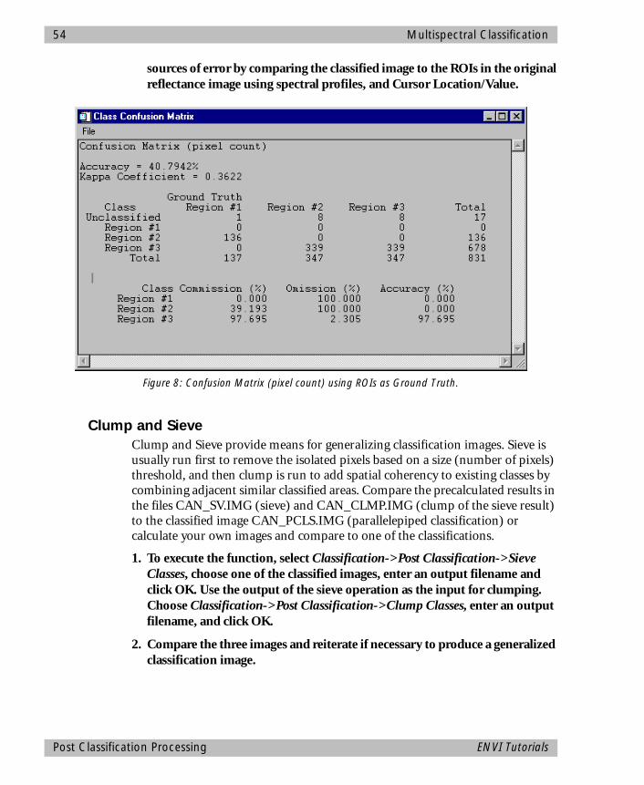
54 Multispectral Classification
sources of error by comparing the classified image to the ROIs in the original reflectance image using spectral profiles, and Cursor Location/Value.
Clump and SieveClump and Sieve provide means for generalizing classification images. Sieve is usually run first to remove the isolated pixels based on a size (number of pixels) threshold, and then clump is run to add spatial coherency to existing classes by combining adjacent similar classified areas. Compare the precalculated results in the files CAN_SV.IMG (sieve) and CAN_CLMP.IMG (clump of the sieve result) to the classified image CAN_PCLS.IMG (parallelepiped classification) or calculate your own images and compare to one of the classifications.
1. To execute the function, select Classification->Post Classification->Sieve Classes, choose one of the classified images, enter an output filename and click OK. Use the output of the sieve operation as the input for clumping. Choose Classification->Post Classification->Clump Classes, enter an output filename, and click OK.
2. Compare the three images and reiterate if necessary to produce a generalized classification image.
Figure 8: Confusion Matrix (pixel count) using ROIs as Ground Truth.
Post Classification Processing ENVI Tutorials

Multispectral Classification 55
Combine ClassesThe Combine Classes function provides an alternative method for classification generalization. Similar classes can be combined to form one or more generalized classes.
1. Examine the precomputed image CAN_COMB.IMG or perform your own combinations as described below.
2. Select Classification->Post Classification->Combine Classes and choose Region 3 to combine with Unclassified, click on Add Combination, and then OK in the Combine Classes Parameters dialog. Enter an output filename and click OK.
3. Compare the combined class image to the classified images and the generalized classification image using image linking and dynamic overlays.
Edit Class ColorsWhen a classification image is displayed, you can change the color associated with a specific class by editing the class colors.
1. Select Functions->Display Enhancements->Color Tables->Class Color Mapping in the Main Image Display window.
2. Click on one of the class names in the Class Color Mapping dialog and change the color by dragging the appropriate color sliders or entering the desired data values. Changes are applied to the classified image immediately. To make the changes permanent, select File->Save Changes in the dialog.
Overlay ClassesOverlay classes allows the user to place the key elements of a classified image as a color overlay on a grayscale or RGB image.
1. Examine the precalculated image CAN_OVR.IMG or create your own overlay(s) from the CAN_TMR.IMG reflectance image and one of the classified images above.
2. Select Classification->Post Classification->Overlay Classes from the ENVI Main menu and use CAN_COMB.IMG as the classification input and CAN_TMR.IMG band 3 as the RGB image layers (the same band for RGB). Click OK and then choose Region #1 and Region #2 to overlay on the image. Enter an output name and click OK to complete the overlay.
3. Load the overlay image into an image display and compare with the classified image and the reflectance image using linking and dynamic overlays.
ENVI Tutorials Post Classification Processing
56 Multispectral Classification
Classes to Vector LayersLoad the precalculated vector layers onto the grayscale reflectance image for comparison to raster classified images, or execute the function and convert one of the classification images to vector layers.
1. To Load the precalculated vector layers produced from the clumped classification image above, select Functions->Overlays->Vector Layers in the Main Image Display with the clumped image CAN_CLMP.IMG displayed.
2. Choose File->Open Vector File->ENVI Vector File in the Display Vector Parameters dialog and choose the files CAN_V1.EVF AND CAN_V2.EVF. Click on Apply to load the vector layers onto the image display.
3. The vectors derived from the classification polygons will outline the raster classified pixels.
1. To complete your own Classification to Vector conversion, select Classification->Post Classification->Classes to Vector Layers and choose the generalized image CAN_CLMP.IMG as the Raster to Vector input image.
2. Select Region #1 and Region #2, enter the root name “CANRTV” and click OK to begin the conversion.
3. Select the two regions in the Available Vectors List by clicking in the appropriate check boxes and click on Load Selected at the bottom of the dialog.
4. Choose the correct display number in the Load Vector dialog for the grayscale reflectance image and the vector layers will be loaded into the Display Vector Parameters Dialog. Click Apply to display the vectors over the image. Use Edit Layer to change the colors and fill of the vector layers to make them more visible.
Classification Keys Using AnnotationENVI provides annotation tools to put classification keys on images and in map layouts. The classification keys are automatically generated.
1. Choose Functions->Overlays->Annotation in the Main Image display window for either one of the classified images, or for the image with the vector overlay.
2. Select Object->Map Key to start annotating the image. You can edit the key characteristics by clicking on the Edit Map Key Items button in the annotation dialog and changing the desired characteristics. Click and drag the map key using the left mouse button in the display to place the key. Click
Classes to Vector Layers ENVI Tutorials
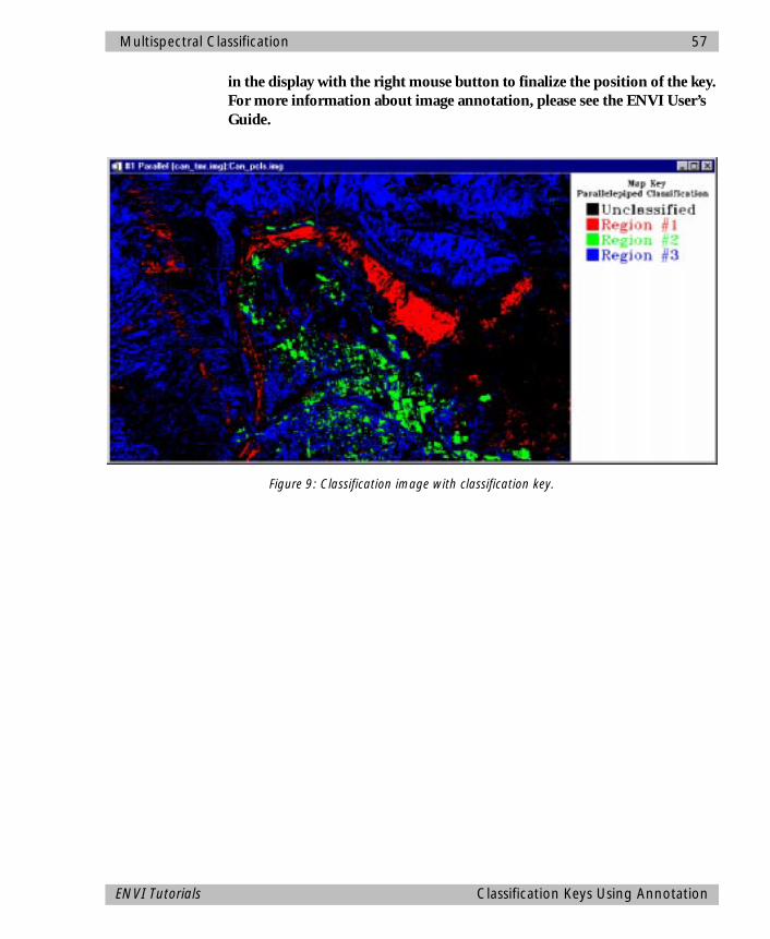
Multispectral Classification 57
in the display with the right mouse button to finalize the position of the key. For more information about image annotation, please see the ENVI User’s Guide.
Figure 9: Classification image with classification key.
ENVI Tutorials Classification Keys Using Annotation

58 Multispectral Classification
Classification Keys Using Annotation ENVI Tutorials
ENVI Tutorial #3
Image Georeferencing and Registration
The following topics are covered in this tutorial:
Overview of This Tutorial ........................................................................................60Background - Georeferenced Images in ENVI ..........................................................61Examine Georeferenced Data and Output Image-Map............................................62Image-to-Image Registration...................................................................................68Image-to-Map Registration .....................................................................................73IHS Merge of Different Resolution Georeferenced Data Sets ....................................78
59
60 Image Georeferencing and Registration
Overview of This TutorialThis tutorial provides basic information about Georeferenced images in ENVI and Image-to-Image and Image-to-Map Registration using ENVI. It covers step-by-step procedures for successful registration, discusses how to make image-maps using ENVI and illustrates the use of multi-resolution data for IHS Sharpening. It is designed to provide a starting point to users trying to conduct image registration. It assumes that you are already familiar with general image-registration and resampling concepts. This tutorial is designed to be completed in about 1 to 2 hours.
Files Used in This TutorialYou must have the ENVI CD-ROM mounted on your system to access the files used by this tutorial or copy the files to your disk.
The files used in this tutorial are contained in the BLDR_REG subdirectory of the tutorial data directory on the ENVI CD-ROM.
Required FilesThe files listed below, along with associated .hdr files, are required to run this exercise.
BLDR_SP.IMG Boulder SPOT Georefer-enced Image Subset
BLDR_SP.HDR ENVI Header for Above
BLDR_SP.GRD Boulder SPOT Map Grid Parameters
BLDR_SP.ANN Boulder SPOT Map Anno-tation
BLDR_TM.IMG Non-Georeferenced Boulder TM Data
BLDR_TM.HDR ENVI Header for Above
BLDR_TM.PTS GCPs for TM-SPOT Image-to-Image Registration
BLDRTM_M.PTS GCPs for TM-Map Regis-tration
BLDR_RD.DLG Boulder Roads DLG
BLDRTMSP.GRD Merged TM-SPOT Map Grids
Topics Covered in This TutorialExamine Georeferenced SPOT Data and Output Image-Map• Open and Display SPOT Data• Edit Map Info in ENVI Header• Cursor Location/Value• Overlay Map Grid• Overlay Map Annotation• Output to Postscript
Image-to-Image Registration• Open and Display TM Data• Cursor Location/Value• Start Registration and Load GCPs• Predict and Add New GCPs• Warp using RST and Nearest
Neighbor, Bilinear Interpolation, and Cubic Convolution and Compare Results using Dynamic Overlay
• Examine Map Coordinates Using Cursor Location/Value
• Warp using RST, Polynomial, Triangulation and Compare Results Using Dynamic Overlay
• Close All Files
Image-to-Map Registration• Display TM Data• Select Image-to-Map Registration
and Restore GCPs• Add GCPs Using Vector Display of
DLGs• Warp Image using RST and Cubic
Convolution• Display Result and Evaluate using
Cursor Location/Value
IHS Merge of Different Resolution Georeferenced Data Sets• Display 30 m TM Color Composite• Display 10 m SPOT Data• Perform IHS Sharpening• Display 10 m Color Image• Overlay Map Grid• Overlay Annotation• Output Image Map
Overview of This Tutorial ENVI Tutorials
Image Georeferencing and Registration 61
BLDRTMSP.ANN Merged TM-SPOT Annotation
Files Generated During This TutorialBLDR_TM1.WRP Image-to-Image Result Using RST and Nearest
Neighbor
BLDR_TM1.HDR ENVI Header for Above
BLDR_TM2.WRP Image-to-Image Result Using RST and BilinearInterpolation
BLDR_TM2.HDR ENVI Header for Above
BLDR_TM3.WRP Image-to-Image Result Using RST and CubicConvolution
BLDR_TM3.HDR ENVI Header for Above
BLDR_TM4.WRP Image-to-Image Result Using 1st degree poly-nomial and Cubic Convolution
BLDR_TM4.HDR ENVI Header for Above
BLDR_TM5.WRP Image-to-Image ResultUsing Delaunay Triangulation and Cubic Con-volution
BLDR_TM5.HDR ENVI Header for Above
BLDR_TM5.HDR ENVI Header for Above
BLDRTM_M.IMG Image-to-Map Result using RST and Cubic Con-volution for the Boulder TM data
BLDRTM_M.HDR ENVI Header for Above
BLDRTMSP.IMG Bouler TM/SPOT sharpening result using IHSsharpening, 10 meter pixels.
BLDRTMSP.HDR ENVI Header for Above
Background - Georeferenced Images in ENVIENVI provides full support for georeferenced images in numerous predefined map projections including UTM and State Plane. In addition, ENVI’s user-configurable map projections allow construction of custom map projections utilizing 6 basic projection types, over 35 different ellipsoids and more than 100 datums to suit most map requirements.
ENVI map projection parameters are stored in an ASCII text file “map_proj.txt” that can be modified by ENVI map projection utilities or edited directly by the
ENVI Tutorials Background - Georeferenced Images in ENVI
62 Image Georeferencing and Registration
user. The information in this file is used in the ENVI Header files associated with each image and allows simple association of a “Magic Pixel” location with known map projection coordinates. Selected ENVI functions can then use this information to work with the image in georeferenced data space.
ENVI’s image registration and geometric correction utilities allow you to reference pixel-based images to geographic coordinates and/or correct them to match base image geometry. Ground control points (GCPs) are selected using the full resolution (Main Image) and Zoom windows for both image-to-image and image-to-map registration. Coordinates are displayed for both base and uncorrected image GCPs, along with error terms for specific warping algorithms. Next GCP point prediction allows simplified selection of GCPs.
Warping is performed using resampling, scaling and translation (RST), polynomial functions (of order 1 through n), or Delaunay triangulation. Resampling methods supported include nearest-neighbor, bilinear interpolation, and cubic convolution. Comparison of the base and warped images using ENVI’s multiple Dynamic Overlay capabilities allows quick assessment of registration accuracy.
The following sections provide examples of some of the map-based capabilities built into ENVI. Consult the ENVI User’s Guide for additional information.
Examine Georeferenced Data and Output Image-MapThis portion of the exercise will familiarize you with the use of georeferenced data in ENVI, allow you to construct an image-map complete with map grids and annotation, and produce an output image.
Start ENVIBefore attempting to start the program, ensure that ENVI is properly installed as described in the installation guide.
♦ To open ENVI in Unix, enter “envi” at the UNIX command line.
♦ To open ENVI from a Windows or Macintosh system, double-click on the ENVI icon.
The ENVI Main Menu appears when the program has successfully loaded and executed.
Open and Display SPOT DataTo open the Georeferenced SPOT data:
1. Select File->Open Image File on the ENVI Main Menu.
Examine Georeferenced Data and Output Image-Map ENVI Tutorials

Image Georeferencing and Registration 63
Note On some platforms you must hold the left mouse button down to display the submenus from the Main Menu.
2. When the Enter Input Data File file-selection dialog appears, navigate to the BLDR_REG subdirectory of the ENVI tutorial data directory and select the file BLDR_SP.IMG from the list.
3. Click “OK”.
4. When the Available Bands List dialog appears, click on the grayscale toggle button and select the SPOT band listed at the top of the dialog by clicking on the band with the left mouse button.
The band you have chosen will be displayed in the field marked “Selected Band:”.
5. Click “Load Band” to load the image into a new display.
Edit Map Info in ENVI Header1. Select File->Edit ENVI Header.
2. When the Edit Header Input dialog appears, select the file BLDR_SP.IMG and click “OK”.
3. When the Header Information dialog appears, select Edit Attributes->Map Info to start the Map Information dialog.
This dialog lists the basic map information used by ENVI in georeferencing. The image coordinates correspond to the “Magic Pixel” used by ENVI as the starting point for the map coordinate system. Because ENVI knows the map projection, pixel size, and map projection parameters based on this header information and the map projection text file, it is able to calculate the geographic coordinates of any pixel in the image. Coordinates can be entered in either map coordinates or geographic coordinates.
4. Click on the toggle arrow next to the text “UTM Zone 13 North” to see the latitude/longitude coordinates for these map projection coordinates.
ENVI makes this conversion on-the-fly.
5. Click on the “DMS<->DD” button to toggle between Degrees Minutes, Seconds, and Decimal Degrees.
6. Click “Cancel” to exit the Map Information dialog.
7. Click “Cancel” to exit Edit ENVI Header dialog.
ENVI Tutorials Examine Georeferenced Data and Output Image-Map
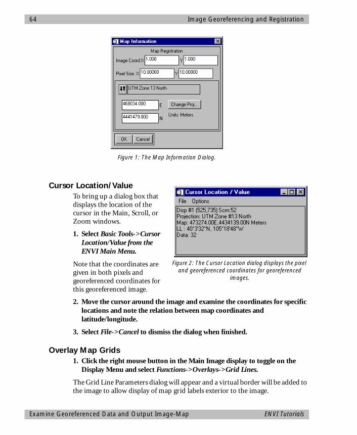
64 Image Georeferencing and Registration
Cursor Location/Value
To bring up a dialog box that displays the location of the cursor in the Main, Scroll, or Zoom windows.
1. Select Basic Tools->Cursor Location/Value from the ENVI Main Menu.
Note that the coordinates are given in both pixels and georeferenced coordinates for this georeferenced image.
2. Move the cursor around the image and examine the coordinates for specific locations and note the relation between map coordinates and latitude/longitude.
3. Select File->Cancel to dismiss the dialog when finished.
Overlay Map Grids1. Click the right mouse button in the Main Image display to toggle on the
Display Menu and select Functions->Overlays->Grid Lines.
The Grid Line Parameters dialog will appear and a virtual border will be added to the image to allow display of map grid labels exterior to the image.
Figure 2: The Cursor Location dialog displays the pixel and georeferenced coordinates for georeferenced
images.
Figure 1: The Map Information Dialog.
Examine Georeferenced Data and Output Image-Map ENVI Tutorials
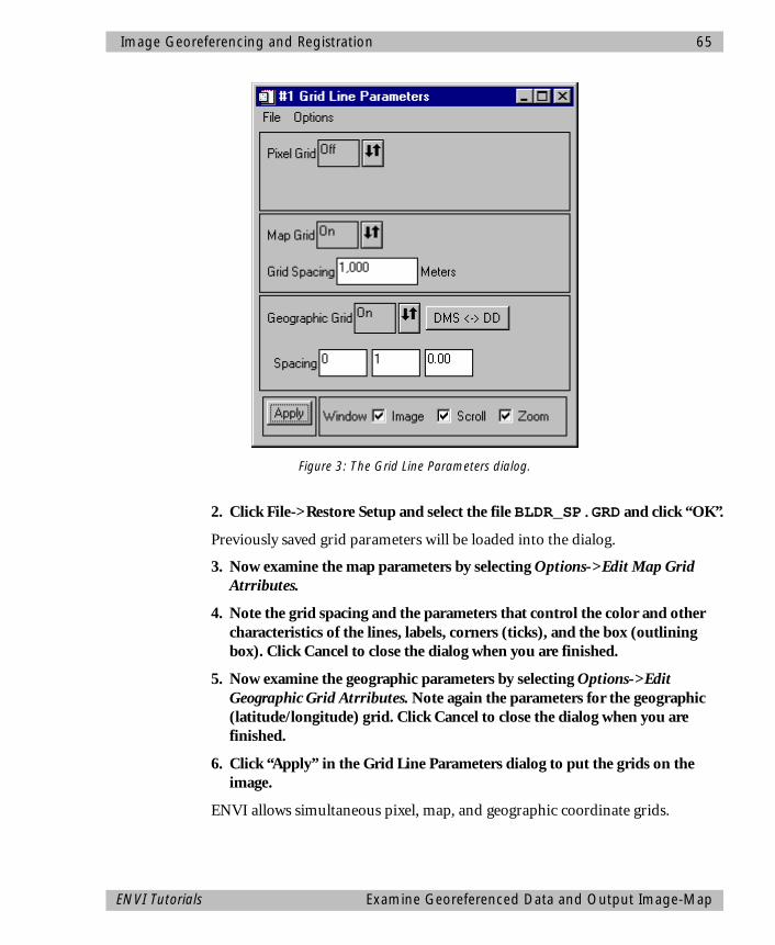
Image Georeferencing and Registration 65
2. Click File->Restore Setup and select the file BLDR_SP.GRD and click “OK”.
Previously saved grid parameters will be loaded into the dialog.
3. Now examine the map parameters by selecting Options->Edit Map Grid Atrributes.
4. Note the grid spacing and the parameters that control the color and other characteristics of the lines, labels, corners (ticks), and the box (outlining box). Click Cancel to close the dialog when you are finished.
5. Now examine the geographic parameters by selecting Options->Edit Geographic Grid Atrributes. Note again the parameters for the geographic (latitude/longitude) grid. Click Cancel to close the dialog when you are finished.
6. Click “Apply” in the Grid Line Parameters dialog to put the grids on the image.
ENVI allows simultaneous pixel, map, and geographic coordinate grids.
Figure 3: The Grid Line Parameters dialog.
ENVI Tutorials Examine Georeferenced Data and Output Image-Map
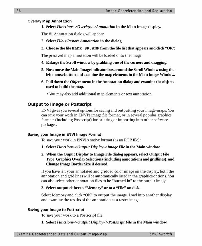
66 Image Georeferencing and Registration
Overlay Map Annotation1. Select Functions->Overlays->Annotation in the Main Image display.
The #1 Annotation dialog will appear.
2. Select File->Restore Annotation in the dialog.
3. Choose the file BLDR_SP.ANN from the file list that appears and click “OK”.
The presaved map annotation will be loaded onto the image.
4. Enlarge the Scroll window by grabbing one of the corners and dragging.
5. Now move the Main Image indicator box around the Scroll Window using the left mouse button and examine the map elements in the Main Image Window.
6. Pull down the Object menu in the Annotation dialog and examine the objects used to build the map.
• You may also add additional map elements or text annotation.
Output to Image or PostscriptENVI gives you several options for saving and outputting your image-maps. You can save your work in ENVI’s image file format, or in several popular graphics formats (including Postscript) for printing or importing into other software packages.
Saving your Image in ENVI Image FormatTo save your work in ENVI’s native format (as an RGB file):
1. Select Functions->Output Display->Image File in the Main window.
2. When the Ouput Display to Image File dialog appears, select Output File Type, Graphics Overlay Selections (including annotations and gridlines), and Change Image Border Size if desired.
If you have left your annotated and gridded color image on the display, both the annotation and grid lines will be automatically listed in the graphics options. You can also select other annotation files to be “burned in” to the output image.
3. Select output either to “Memory” or to a “File” on disk.
Select Memory and click “OK” to output the image. Load into another display and examine the results of the annotation as a raster image.
Saving your Image to PostscriptTo save your work to a Postscript file:
1. Select Functions->Output Display- >Postscript File in the Main window.
Examine Georeferenced Data and Output Image-Map ENVI Tutorials
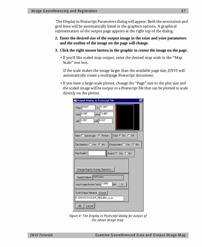
Image Georeferencing and Registration 67
The Display to Postscript Parameters dialog will appear. Both the annotation and grid lines will be automatically listed in the graphics options. A graphical representation of the output page appears at the right top of the dialog.
2. Enter the desired size of the output image in the xsize and ysize parameters and the outline of the image on the page will change.
3. Click the right mouse button in the graphic to center the image on the page.
• If you’d like scaled map output, enter the desired map scale in the “Map Scale” text box.
If the scale makes the image larger than the available page size, ENVI will automatically create a multipage Postscript document.
• If you have a large-scale plotter, change the “Page” size to the plot size and the scaled image will be output to a Postscript file that can be plotted to scale directly on the plotter.
Figure 4: The Display to Postscript dialog for output of the above image map.
ENVI Tutorials Examine Georeferenced Data and Output Image-Map

68 Image Georeferencing and Registration
• Clicking “OK” saves the image. Create the Postscript file only if you can print color output and print the file using your standard operating system proce-dures for printing Postscript output.
• If you can’t print color output, click “Cancel” to cancel the output operation.
Direct PrintingENVI also allows direct printing to devices supported by your operating system.
1. Select Output Display->Printer and follow your standard printing procedures.
For example in Microsoft Windows, you would select the Printer from the pulldown Name: menu, change the properties as desired, and click on OK to print the image.
2. Once you have selected all of the parameters and clicked OK, a dialog appears to allow you to set additional basic ENVI printing parameters. Set these as desired and click OK to begin printing.
Image-to-Image RegistrationThis section of the tutorial will take you step-by-step through an Image-to-Image registration. The georeferenced SPOT image will be used as the Base image, and a pixel-based Landsat TM image will be warped to match the SPOT.
Open and Display Landsat TM Image File1. Select File->Open Image File.
2. When the Enter Input Data File file-selection dialog appears, navigate to the BLDR_REG subdirectory of the ENVI tutorial data directory and select the file BLDR_TM.IMG from the list.
3. Click “OK” to load the TM image bands into the Available Bands List.
4. Click on Band 3, the “New” button and then “Load Band” to load the TM band 3 image into a new display.
Display the Cursor Location/ValueTo bring up a dialog box that displays the location of the cursor in the Main, Scroll, or Zoom windows:
1. Select Basic Tools->Cursor Location / Value on the ENVI Main Menu.
Image-to-Image Registration ENVI Tutorials
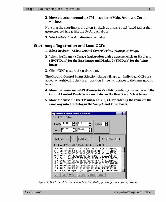
Image Georeferencing and Registration 69
2. Move the cursor around the TM image in the Main, Scroll, and Zoom windows.
Note that the coordinates are given in pixels as this is a pixel-based rather than georeferenced image like the SPOT data above.
3. Select File->Cancel to dismiss the dialog.
Start Image Registration and Load GCPs1. Select Register ->Select Ground Control Points->Image-to-Image.
2. When the Image-to-Image Registration dialog appears, click on Display 1 (SPOT Data) for the Base image and Display 2 (TM Data) for the Warp image.
3. Click “OK” to start the registration.
The Ground Control Points Selection dialog will appear. Individual GCPs are added by positioning the cursor position in the two images to the same ground location.
4. Move the cursor in the SPOT image to 753, 826 by entering the values into the Ground Control Points Selection dialog in the Base X and Y text boxes.
5. Move the cursor in the TM image to 331, 433 by entering the values in the same way into the dialog in the Warp X and Y text boxes.
Figure 5: The Ground Control Points Selection dialog for image-to-image registration.
ENVI Tutorials Image-to-Image Registration

70 Image Georeferencing and Registration
6. Examine the locations in the two Zoom windows and adjust the locations if necessary by clicking the middle mouse button in each Zoom window at the desired locations.
Note that sub-pixel positioning is supported in the Zoom windows. The larger the zoom factor, the finer the positioning capabilities.
7. Click “Add” to add the GCP to the list. Try this for a few points to get the feel of selecting GCPs.
Note the list of actual and predicted points in the dialog. Once you have at least 4 points, the RMS error is reported.
8. Now select GCPs->Clear GCPs in the dialog to clear all of your points.
9. Choose File->Restore GCPs from ASCII in the dialog and click on the file name BLDR_TM.PTS.
10. Click “OK” to load a list of pre-saved GCPs.
11. Click on individual GCPs in the list and examine the locations of the points in the two images, the actual and predicted coordinates, and the RMS error.
Edit, On/Off, Delete, Update, and Predict GCPsThe following descriptions are provided for information only. Perform only the numbered Predict GCP button functions.
• Clicking on the “Edit” button adjusts the position of individual GCPs. Either enter a new pixel location, or move the position pixel-by-pixel using the direction arrows in the dialog.
• Clicking on the “On/Off” button removes selected GCPs from consideration in the Warp model and RMS calculations. These GCPs aren’t actually deleted, just disregarded, and can be toggled back on using the “On/Off button”.
• Clicking on the “Delete” button removes a GCP from the list.
• Positioning the cursor location in the two zoom boxes and clicking the “Update” button updates the selected GCP to the current cursor locations.
• The “Predict” button allows prediction of new GCPs based on the current warp model.
1. Try positioning the cursor at a new location in the SPOT image. Click on the “Predict” button and the cursor position in the TM image will be moved to match its predicted location based on the warp model.
2. The exact position can then be interactively refined by moving the pixel location slightly in the TM data.
Image-to-Image Registration ENVI Tutorials

Image Georeferencing and Registration 71
3. Click “Add” to add the new GCP to the list.
Warp ImagesImages can be warped from the displayed band, or multiband images can be warped all bands at once. We will warp only the displayed band.
1. Select Options->Warp Displayed Band in the Ground Control Points Selection dialog.
2. When the Registration Parameters dialog appears, select “RST” as the Warp Method and “Nearest Neighbor” resampling.
3. Enter the filename BLDRTM_1.WRP and click “OK”.
The warped image will be listed in the Available Bands list when the warp is completed.
4. Now repeat using RST warping with both Bilinear Interpolation, and Cubic Convolution.
5. Output the results to BLDR_TM2.WRP and BLDR_TM3.WRP, respectively.
6. Perform both a 1st degree polynomial warp and a Delaunay Triangulation warp using Cubic Convolution.
7. Output the results to BLDR_TM4.WRP and BLDR_TM5.WRP respectively.
Compare Warp Results Using Dynamic Overlays1. Click on the original TM band 3 image name BLDR_TM.IMG in the Available
Bands list and then select File->Close from the menu bar.
2. In the subsequent dialog, click “Yes” to close the associated image file.
3. Load BLDRTM_1.WRP into a new image display by clicking on the band name in the Available Bands List, clicking “New”, and clicking “Load Band”.
4. Click the right mouse button in the Main window and select Functions > Link > Link Displays.
5. Click “OK” in the Link Displays dialog to link the SPOT and the registered TM image.
6. Now compare the SPOT and the TM images using the Dynamic Overlay by dragging in the Main Image display with the left mouse button depressed.
7. Load BLDRTM_2.WRP and BLDRTM_3.WRP into new displays and use the image linking and dynamic overlays to compare the effect of the three different resampling methods: nearest neighbor, bilinear interpolation, and cubic convolution.
ENVI Tutorials Image-to-Image Registration
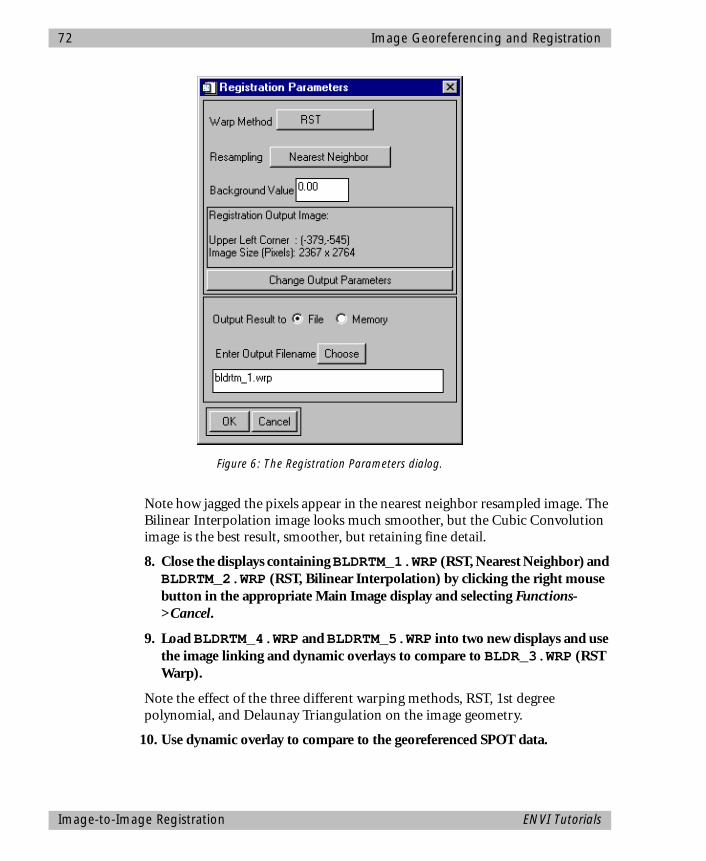
72 Image Georeferencing and Registration
Note how jagged the pixels appear in the nearest neighbor resampled image. The Bilinear Interpolation image looks much smoother, but the Cubic Convolution image is the best result, smoother, but retaining fine detail.
8. Close the displays containing BLDRTM_1.WRP (RST, Nearest Neighbor) and BLDRTM_2.WRP (RST, Bilinear Interpolation) by clicking the right mouse button in the appropriate Main Image display and selecting Functions->Cancel.
9. Load BLDRTM_4.WRP and BLDRTM_5.WRP into two new displays and use the image linking and dynamic overlays to compare to BLDR_3.WRP (RST Warp).
Note the effect of the three different warping methods, RST, 1st degree polynomial, and Delaunay Triangulation on the image geometry.
10. Use dynamic overlay to compare to the georeferenced SPOT data.
Figure 6: The Registration Parameters dialog.
Image-to-Image Registration ENVI Tutorials

Image Georeferencing and Registration 73
Examine Map CoordinatesTo bring up the Cursor Location/Value dialog:
1. Select Basic Tools->Cursor Location/Value.
2. Browse the georeferenced data sets and note the effect of the different resampling and warp methods on the data values.
3. Select File->Cancel in to close the dialog.
Close All Files
• To close all of the data files, select File ->Close All Files from the ENVI Main Menu.
Image-to-Map RegistrationThis section of the tutorial will take you step-by-step through an Image-to-Map registration. Many of the procedures are similar to image-to-image and will not be discussed in detail. The map coordinates picked from the georeferenced SPOT image and a vector Digital Line Graph (DLG) will be used as the Base, and the pixel-based Landsat TM image will be warped to match the map data.
Open and Display Landsat TM Image File1. Select File->Open Image File.
2. When the Enter Input Data File dialog appears, navigate to the BLDR_REG subdirectory of the ENVI tutorial data directory and select the file BLDR_TM.IMG from the list.
3. Click “OK” to load the TM image bands into the Available Bands List. Click on Band 3, the “New” button and then “Load Band” to load the TM band 3 image into a new display.
Select Image-to-Map Registration and Restore GCPs1. Select Register->Select Ground Control Points->Image-to-Map.
2. When the Image-to-Map Registration dialog appears, click on “UTM” as the map projection to use and enter 13 for the “Zone”.
3. Leave the pixel size at 30 m and click “OK” to start the registration.
The Ground Control Points Selection dialog will appear as for image-to-image registration.
ENVI Tutorials Image-to-Map Registration
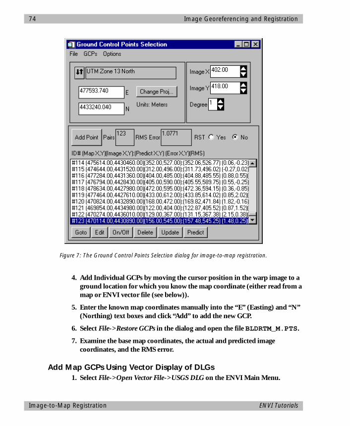
74 Image Georeferencing and Registration
4. Add Individual GCPs by moving the cursor position in the warp image to a ground location for which you know the map coordinate (either read from a map or ENVI vector file (see below)).
5. Enter the known map coordinates manually into the “E” (Easting) and “N” (Northing) text boxes and click “Add” to add the new GCP.
6. Select File->Restore GCPs in the dialog and open the file BLDRTM_M.PTS.
7. Examine the base map coordinates, the actual and predicted image coordinates, and the RMS error.
Add Map GCPs Using Vector Display of DLGs1. Select File->Open Vector File->USGS DLG on the ENVI Main Menu.
Figure 7: The Ground Control Points Selection dialog for image-to-map registration.
Image-to-Map Registration ENVI Tutorials
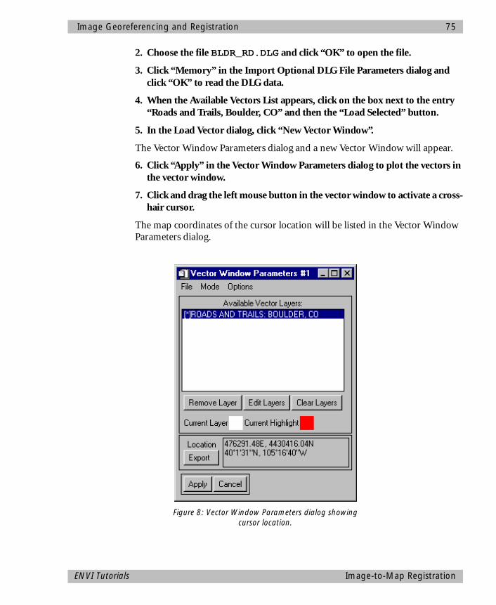
Image Georeferencing and Registration 75
2. Choose the file BLDR_RD.DLG and click “OK” to open the file.
3. Click “Memory” in the Import Optional DLG File Parameters dialog and click “OK” to read the DLG data.
4. When the Available Vectors List appears, click on the box next to the entry “Roads and Trails, Boulder, CO” and then the “Load Selected” button.
5. In the Load Vector dialog, click “New Vector Window”.
The Vector Window Parameters dialog and a new Vector Window will appear.
6. Click “Apply” in the Vector Window Parameters dialog to plot the vectors in the vector window.
7. Click and drag the left mouse button in the vector window to activate a cross-hair cursor.
The map coordinates of the cursor location will be listed in the Vector Window Parameters dialog.
Figure 8: Vector Window Parameters dialog showing cursor location.
ENVI Tutorials Image-to-Map Registration
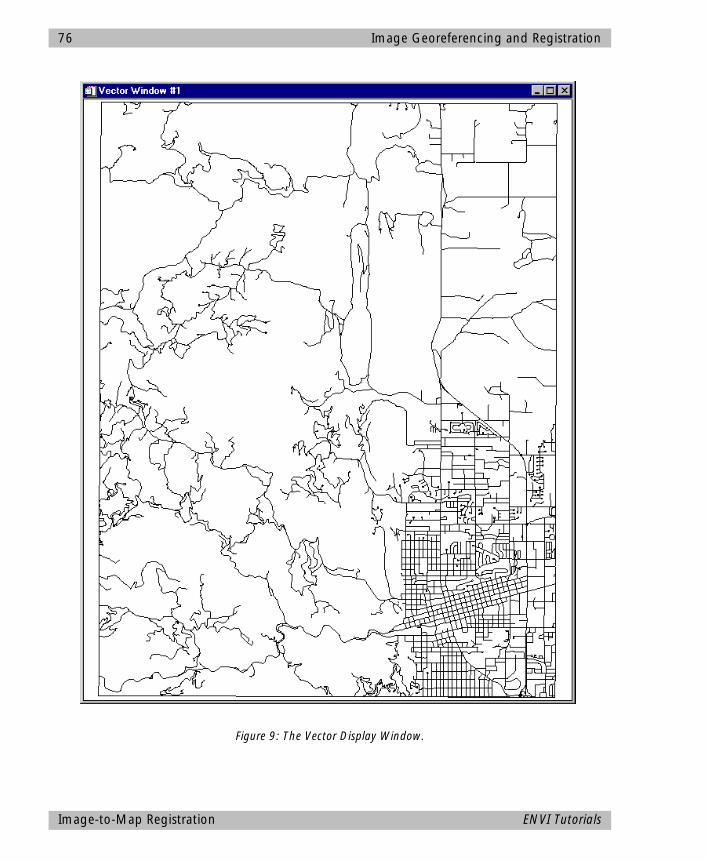
76 Image Georeferencing and Registration
Figure 9: The Vector Display Window.
Image-to-Map Registration ENVI Tutorials
Image Georeferencing and Registration 77
8. Position the image cursor on the road intersection at 402, 418 in the image display by selecting Functions->-Interactive Analysis->Pixel Locator, entering the value, and clicking Apply.
Note that sub-pixel positioning accuracy is again available in the Zoom window.
9. Position the Vector cursor at the road intersection at 4775593.74, 4433240.0 (40d 3m 3s N, -105d 15m 45s W) by clicking and dragging with the left mouse button and releasing when the circle at the cross-hair intersection overlays the intersection of interest.
10. Click “Export” in the Vector Window Params #1 dialog, and these mapcoordinates will appear in the Ground Control Points Selection dialog.
11. Click “Add” to add the map-coordinate/image pixel pair and observe thechange in RMS error.
Warp Image using RST and Cubic Convolution1. In the Ground Control Points Selection dialog, select Options->Warp File.
2. Click on the file name BLDR_TM.IMG and click “OK” to select all 6 TM bands for warping.
3. Choose RST and Cubic Convolution resampling in the Registration Parameters dialog.
4. Enter the output file name BLDRTM_M.IMG in the output file text box.
5. Change the background value to 255.
6. Click “OK” to start the image-to-map warp.
Display Result and Evaluate using Cursor Location/Value1. Click on the RGB radio button in the Available Bands List followed by
clicking on bands 4, 3, and 2 (RGB) of the warped image.
2. Click “New” and then “Load RGB” to load the TM warped color image.
Note the skew resulting from removal of the Landsat TM orbit direction. This image is georeferenced, but at 30 meter resolution versus the 10 meter resolution provided by the SPOT image.
• If desired, load the SPOT image into a new display window and compare the image geometries and scale.
ENVI Tutorials Image-to-Map Registration
78 Image Georeferencing and Registration
Close Selected FilesYou can leave BLDRTM_M.IMG and BLDR_SP.IMG open as you will use these files in the next exercise.
1. Click on any other file names in the Available Bands list and click select File->Close Selected File to close these images.
2. Click “Cancel” in the Vector Window Params #1 dialog to close the Vector Window.
3. Select File->Cancel in the Available Vectors list to close that dialog.
4. Select File->Cancel in the Ground Control Points Selection dialog to close that dialog. Save the GCPs if desired.
IHS Merge of Different Resolution Georeferenced Data SetsThis portion of the tutorial describes the procedures for merging two georeferenced data sets containing different pixel sizes. We will use the TM color-composite image registered above as the low-resolution color image and the georeferenced SPOT image as the high resolution image. The result is a color composite image with enhanced spatial resolution.
Display 30 m TM Color Composite1. If you closed the registered TM image, reopen the file BLDRTM_M.IMG.
2. Click on the “RGB” toggle button in the Available Bands List, and load bands 4, 3, and 2 (RGB) into a new display.
Display 10 m SPOT Data1. If you closed the SPOT image, open the file BLDR_SP.IMG
2. Click on the “Grayscale” toggle button in the Available Bands List, the “New” button, and the “Load Band” button to load the SPOT data into a new display.
Compare with the TM data above and note the similar image geometry, but different spatial coverage and image scales.
Perform IHS Sharpening1. Select Transforms->Image Sharpening->IHS from the ENVI Main Menu.
IHS Merge of Different Resolution Georeferenced Data Sets ENVI Tutorials
Image Georeferencing and Registration 79
2. If you have the color image displayed, choose the appropriate display in the Select Input RGB dialog. Otherwise, choose bands 4, 3, and 2 from the TM Image in the Select Input RGB Input Bands dialog and click OK.
3. Choose the SPOT image in the High Resolution Input File dialog and click “OK”.
4. Enter the output file name BLDRTMSP.IMG and click “OK” in the IHS Sharpening Parameters dialog.
A processing status box will appear and the new image will be listed in the Available Bands List when the processing is completed.
Display 10 m Color Image1. Load the enhanced color image into a new display by selecting the RGB Color
radio button in the Available Bands List dialog, selecting the R, G, and B bands from the new file from list and clicking “Load RGB” .
Compare the IHS sharpened color image to both the original TM color composite and to the SPOT data.
2. Try the same process using the Color Normalized (Brovey) Transform by selecting Transforms->Image Sharpening->Color Normalized (Brovey), entering the required file information and clicking OK.
Overlay Map Grid1. Click the right mouse button in the Main Image and select Functions-
>Overlays->Grid Lines.
The Grid Line Parameters dialog will appear and a virtual border will be added to the image to allow display of map grid labels exterior to the image.
2. Select File->Restore Setup, select BLDRTMSP.GRD, and click “OK”.
Previously saved grid parameters will be loaded into the dialog.
3. Click “Apply” to put the grids on the image.
Overlay Annotation1. Select Functions->Overlays->Annotation in the Main Image display.
2. Select File->Restore Annotation in the dialog and choose the file BLDRTMSP.ANN from the file list that appears and click “OK”.
The presaved map annotation will be loaded onto the image.
ENVI Tutorials IHS Merge of Different Resolution Georeferenced Data Sets
80 Image Georeferencing and Registration
• Optionally, enlarge the Scroll window by grabbing one of the corners and dragging.
Output Image Map
• To save your work use the procedures described above for image output. You can:
• Create an image output file.
• Create a Postscript file.
• Use ENVI’s direct printing capabilities to print a copy of the image-map.
End the ENVI SessionThis concludes the Registration Tutorial.
• To quit your ENVI session, click “Quit” or “Exit” on the ENVI Main Menu, then type “exit” at the IDL command prompt.
If you are using ENVI RT, quitting ENVI will take you back to your operating system.
IHS Merge of Different Resolution Georeferenced Data Sets ENVI Tutorials
ENVI Tutorial #4
Mosaicking Using ENVI
The following topics are covered in this tutorial:
Overview of This Tutorial ........................................................................................82Files Used in this Tutorial .........................................................................................82Background - Mosaicking in ENVI ...........................................................................83General Topics ........................................................................................................83Steps for Creating a Pixel-Based Mosaic ..................................................................87Pixel-based Mosaicking Example .............................................................................89Georeferenced Mosaicking Example........................................................................93
81
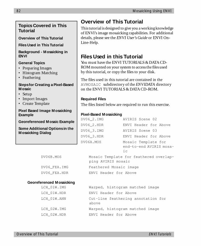
82 Mosaicking Using ENVI
Overview of This TutorialThis tutorial is designed to give you a working knowledge of ENVI’s image mosaicking capabilities. For additional details, please see the ENVI User’s Guide or ENVI On-Line-Help.
Files Used in this TutorialYou must have the ENVI TUTORIALS & DATA CD-ROM mounted on your system to access the files usedby this tutorial, or copy the files to your disk.
The files used in this tutorial are contained in the AVMOSAIC subdirectory of the ENVIDATA directory on the ENVI TUTORIALS & DATA CD-ROM.
Required FilesThe files listed below are required to run this exercise.
Pixel-Based MosaickingDV06_2.IMG AVIRIS Scene 02
DV06_2.HDR ENVI Header for Above
DV06_3.IMG AVIRIS Scene 03
DV06_3.HDR ENVI Header for Above
DV06A.MOS Mosaic Template for end-to-end AVIRIS mosa-ic
DV06B.MOS Mosaic Template for feathered overlap-ping AVIRIS mosaic
DV06_FEA.IMG Feathered Mosaic image
DV06_FEA.HDR ENVI Header for Above
Georeferenced MosaickingLCH_01W.IMG Warped, histogram matched image
LCH_01W.HDR ENVI Header for Above
LCH_01W.ANN Cut-line feathering annotation for above
LCH_02W.IMG Warped, histogram matched image
LCH_02W.HDR ENVI Header for Above
Topics Covered in This Tutorial
Overview of This Tutorial
Files Used in This Tutorial
Background - Mosaicking in ENVI
General Topics• Preparing Images• Histogram Matching• Feathering
Steps for Creating a Pixel-Based Mosaic• Setup• Import Images• Create Template
Pixel Based Image Mosaicking Example
Georeferenced Mosaic Example
Some Additional Options in the Mosaicking Dialog
Overview of This Tutorial ENVI Tutorials
Mosaicking Using ENVI 83
LCH_A.MOS Mosaic Template for Georeferenced Image Mosaicking
LCH_MOS1.IMG Georeferenced mosaic result
LCH_MOS1.HDR ENVI Header for Above
Background - Mosaicking in ENVIMosaicking is the art of combining multiple images into a single composite image. It can be used to combine pixel-based images, to lay out images for publication or map composition, or as a means for combining georeferenced images into an image covering a larger geographic area. ENVI provides interactive capabilities for placing pixel-based images within a mosaic, and automated placement of georeferenced images within a georeferenced output mosaic. The software provides tools for common mosaic requirements such as blending edges (feathering), image border transparency, and histogram matching. ENVI’s Virtual Mosaic capability allows users to optionally create and display mosaics without creating large output files.
General TopicsThe following sections walk you through some of the preparation required to make mosaics in ENVI. The actual start of the exercises begins with the section “Pixel-based Mosaicking Example” or alternatively, for georeferenced mosaicks in the section “ Georeferenced Mosaicking Example”.
Start ENVIBefore attempting to start the program, ensure that ENVI is properly installed as described in the installation guide.
• To open ENVI in Unix, enter “envi” at the UNIX command line.
• To open ENVI from a Windows or Macintosh system, double-click on the ENVI icon.
The ENVI Main Menu appears when the program has successfully loaded and executed.
Preparing ImagesRaw image data can be mosaicked together if desired (ENVI can be used to easily produce multiband mosaics of multiple data types), however, most mosaics are for output and usually require scaling (contrast stretching), and histogram matching to minimize image differences in the output mosaic. The first step in a
ENVI Tutorials Background - Mosaicking in ENVI

84 Mosaicking Using ENVI
mosaic using ENVI is usually to contrast stretch the images. This is done by displaying the bands to be mosaicked and either using one of ENVI’s quick (default) stretches or using ENVI’s interactive contrast stretching capabilities. For mosaics with overlapping images, see the histogram matching description below in the Georeference Image Mosaic example.
1. Start in either the Pixel-Based or the Georeferenced Image Mosaic section below and open the appropriate images by navigating to the AVMOSAIC subdirectory of the ENVIDATA directory on the ENVI TUTORIALS & DATA CD-ROM just as you would in any other application, selecting the desired file from the list and clicking “OK”.
Open the files
2. Select File ->Open Image File.
Note that on some platforms you must hold the left mouse button down to display the submenus from the Main Menu.
An Enter Input Data File file selection dialog appears.
3. Display the image(s) by selecting the desired bands in the Available Bands List and clicking “Load”.
4. Click the right mouse button in the Main Image window to toggle the Functions menu and select Functions->Display Enhancements->Default (quick) Stretches->the desired stretch type, or select Functions->Display Enhancements->Interactive Stretching.
5. Stretch the image to enhance the desired image features and output to memory or a new file by selecting Functions->Output Display->Image File in the Main Display window.
Histogram MatchingWhen mosaicking two or more images that overlap, it is usually necessary to choose a base image and balance grayscales in the rest of the images to match the base image. This is called histogram matching (Richards, 1993). ENVI’s interactive contrast stretching function provides interactive tools to perform histogram matching. The procedure for performing the histogram matching is described below.
The following steps are provided for information and are not to be executed as part of this tutorial.
1. Display the two images to be histogram matched in two display windows.
General Topics ENVI Tutorials

Mosaicking Using ENVI 85
2. Identify the overlap areas, position the zoom windows of both images within the overlap, and resize and/or reposition the Zoom window to cover exactly the same region in both images (try to cover as large an area as possible and a broad range of cover types).
3. Select Functions->Display Enhancements->Interactive Stretching in both Main Display windows.
The Contrast Stretching dialog will appear.
4. Stretch the first or base image to show the desired contrast stretch using any of ENVI’s contrast stretching methods.
5. In the base image Contrast Stretching dialog, choose Histogram_Source->Zoom.
The input and output histograms will be shown for the data in the zoom window.
6. In the second contrast stretching dialog, also select Histogram_Source->Zoom.
7. Also select Stretch_type->Arbitrary in the second dialog.
8. In the base contrast stretching dialog, click the left mouse button on the first letter of the word “Output Histogram”, hold the button down, drag the text to the output histogram of the second contrast stretching dialog, and release the button.
The output histogram from the base image will be applied to the histogram of the second image.
9. Click “Apply” in the second dialog to apply this contrast stretch to the image being histogram matched.
The two stretched images should now have the same grayscale characteristics.
10. Save the contrast stretched images by selecting Functions->Output Display ->Image File in both Main Displays.
11. Select to save the stretched files either to memory or to new output files.
12. Repeat for additional overlapping images as required.
You may want to try the histogram matching yourself for the second part of this tutorial, however, for the purpose of this exercise, the prestretched, histogram-matched images LCH_01W.IMG and LCH_02W.IMG are provided, as input to the georeferenced mosaicking function.
ENVI Tutorials General Topics
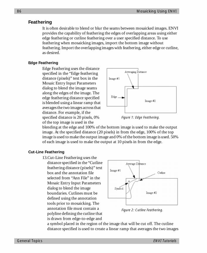
86 Mosaicking Using ENVI
FeatheringIt is often desirable to blend or blur the seams between mosaicked images. ENVI provides the capability of feathering the edges of overlapping areas using either edge feathering or cutline feathering over a user specified distance. To use feathering when mosaicking images, import the bottom image without feathering. Import the overlapping images with feathering, either edge or cutline, as desired.
Edge FeatheringEdge Feathering uses the distance specified in the “Edge feathering distance (pixels)” text box in the Mosaic Entry Input Parameters dialog to blend the image seams along the edges of the image. The edge feathering distance specified is blended using a linear ramp that averages the two images across that distance. For example, if the specified distance is 20 pixels, 0% of the top image is used in the blending at the edge and 100% of the bottom image is used to make the output image. At the specified distance (20 pixels) in from the edge, 100% of the top image is used to make the output image and 0% of the bottom image is used. 50% of each image is used to make the output at 10 pixels in from the edge.
Cut-Line Feathering13.Cut-Line Feathering uses the
distance specified in the “Cutline feathering distance (pixels)” text box and the annotation file selected from “Ann File” in the Mosaic Entry Input Parameters dialog to blend the image boundaries. Cutlines must be defined using the annotation tools prior to mosaicking. The annotation file must contain a polyline defining the cutline that is drawn from edge-to-edge and a symbol placed in the region of the image that will be cut off. The cutline distance specified is used to create a linear ramp that averages the two images
Figure 1: Edge Feathering.
Figure 2: Cutline Feathering.
General Topics ENVI Tutorials
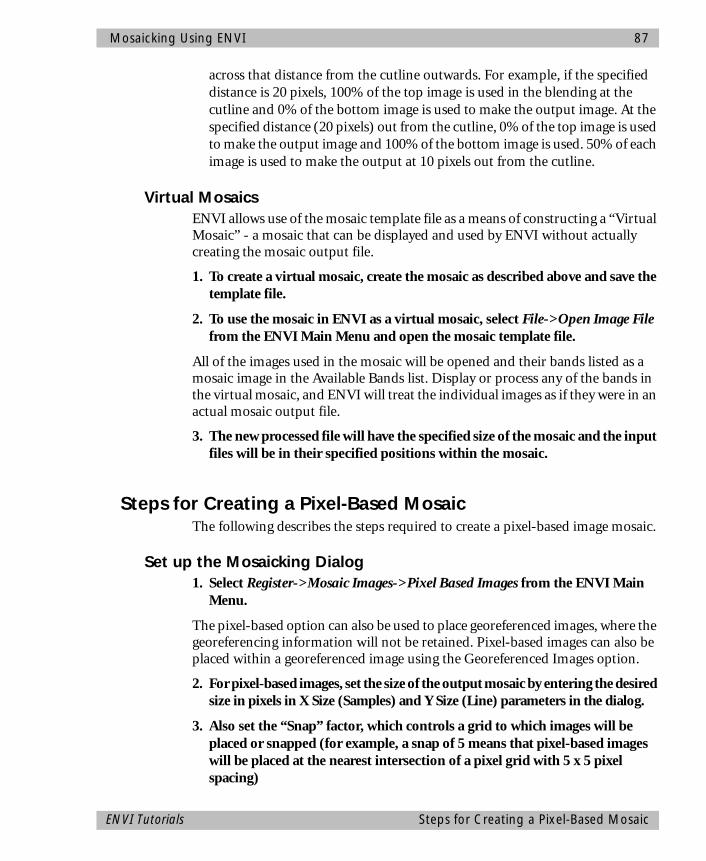
Mosaicking Using ENVI 87
across that distance from the cutline outwards. For example, if the specified distance is 20 pixels, 100% of the top image is used in the blending at the cutline and 0% of the bottom image is used to make the output image. At the specified distance (20 pixels) out from the cutline, 0% of the top image is used to make the output image and 100% of the bottom image is used. 50% of each image is used to make the output at 10 pixels out from the cutline.
Virtual Mosaics ENVI allows use of the mosaic template file as a means of constructing a “Virtual Mosaic” - a mosaic that can be displayed and used by ENVI without actually creating the mosaic output file.
1. To create a virtual mosaic, create the mosaic as described above and save the template file.
2. To use the mosaic in ENVI as a virtual mosaic, select File->Open Image File from the ENVI Main Menu and open the mosaic template file.
All of the images used in the mosaic will be opened and their bands listed as a mosaic image in the Available Bands list. Display or process any of the bands in the virtual mosaic, and ENVI will treat the individual images as if they were in an actual mosaic output file.
3. The new processed file will have the specified size of the mosaic and the input files will be in their specified positions within the mosaic.
Steps for Creating a Pixel-Based MosaicThe following describes the steps required to create a pixel-based image mosaic.
Set up the Mosaicking Dialog1. Select Register->Mosaic Images->Pixel Based Images from the ENVI Main
Menu.
The pixel-based option can also be used to place georeferenced images, where the georeferencing information will not be retained. Pixel-based images can also be placed within a georeferenced image using the Georeferenced Images option.
2. For pixel-based images, set the size of the output mosaic by entering the desired size in pixels in X Size (Samples) and Y Size (Line) parameters in the dialog.
3. Also set the “Snap” factor, which controls a grid to which images will be placed or snapped (for example, a snap of 5 means that pixel-based images will be placed at the nearest intersection of a pixel grid with 5 x 5 pixel spacing)
ENVI Tutorials Steps for Creating a Pixel-Based Mosaic

88 Mosaicking Using ENVI
Import ImagesUse one of the following methods depending on the type of mosaic and whether the images have overlapping areas.
Without Feathering:Images that do not overlap, or images that do not require blending should be imported using the Import File without Feathering option.
1. Select Import->Import File Without Feathering from the menu bar in the Mosaicking dialog.
2. Open and select the desired image and spectrally and/or spatially subset if desired.
The image description will be listed in the dialog, and a graphic representing the image and its position in the mosaic will be displayed in the draw widget within the dialog.
3. Open and import the remaining images in the mosaic in the same fashion.
With Feathering: Images that overlap may require feathering of the overlap areas to avoid obvious seams in the final mosaic.
1. Select Import->Import File With Feathering from the menu bar in the Mosaicking dialog.
If cutline feathering is being used, the cutline must already have been drawn as a polyline annotation and saved to an annotation file as described below.
2. For both cutline and edge feathering, specify a distance over which to feather as described above.
Using feathering will eliminate joins between images, but mosaicking with feathering is compute-intensive and requires a long time to run, especially for large mosaics.
Background Value to Ignore: This option allows image transparency for overlapping images.
1. Select Import->File With Feathering regardless of whether you want to feather the images.
This allows you to set a background value to ignore when images overlay one another.
Steps for Creating a Pixel-Based Mosaic ENVI Tutorials

Mosaicking Using ENVI 89
• If feathering is desired, enter the desired values, however, if feathering is not desired, leave the feathering values set to zero.
2. Enter the data value to be ignored in the labeled text box.
The overlap areas with this value will be transparent, allowing underlying images to show through. This value will also be ignored during the feathering process if selected.
Create Template or Select Apply to Create Output Mosaic1. To create a virtual mosaic (see below), select File->Save Template, enter the
output filename, and click OK. This creates a small text file that describes the mosaic layout.
2. To view this mosaic, select File->Open Image File from the ENVI Main Menu, choose the mosaic template file as the input file and click Open. Click on the mosaic band name in the Available Bands List and then Load Band to automatically get the required images and display the virtual mosaic to the ENVI Image Display.
3. Alternatively, to actually create the mosaic as a new file, select File->Apply in the Mosaic dialog and enter an output filename. The output mosaic is a standard ENVI file and can be displayed using the Available Bands List.
Pixel-based Mosaicking ExampleThis section leads you through creation of Pixel-Based mosaics using ENVI’s mosaicking tools.
1. Start the ENVI Pixel-Based Mosaic function by selecting Register->Mosaic Images->Pixel Based Images from the ENVI Main Menu.
The Pixel-Based Image Mosaicking dialog appears.
Position the images for the Pixel-Based MosaicTo position pixel-based images:
1. Open and import the images DV06_2.IMG and DV06_3.IMG using the methods described above.
2. Specify the mosaic size by entering the 614 for the X Size and 1024 for the Y Size in the text boxes at the top of the Pixel Based Image Mosaicking dialog.
3. Click on the second image in the list of images in the dialog (DV06_3.IMG).
ENVI Tutorials Pixel-based Mosaicking Example
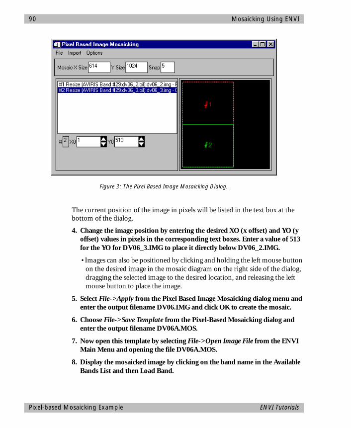
90 Mosaicking Using ENVI
The current position of the image in pixels will be listed in the text box at the bottom of the dialog.
4. Change the image position by entering the desired XO (x offset) and YO (y offset) values in pixels in the corresponding text boxes. Enter a value of 513 for the YO for DV06_3.IMG to place it directly below DV06_2.IMG.
• Images can also be positioned by clicking and holding the left mouse button on the desired image in the mosaic diagram on the right side of the dialog, dragging the selected image to the desired location, and releasing the left mouse button to place the image.
5. Select File->Apply from the Pixel Based Image Mosaicking dialog menu and enter the output filename DV06.IMG and click OK to create the mosaic.
6. Choose File->Save Template from the Pixel-Based Mosaicking dialog and enter the output filename DV06A.MOS.
7. Now open this template by selecting File->Open Image File from the ENVI Main Menu and opening the file DV06A.MOS.
8. Display the mosaicked image by clicking on the band name in the Available Bands List and then Load Band.
Figure 3: The Pixel Based Image Mosaicking Dialog.
Pixel-based Mosaicking Example ENVI Tutorials
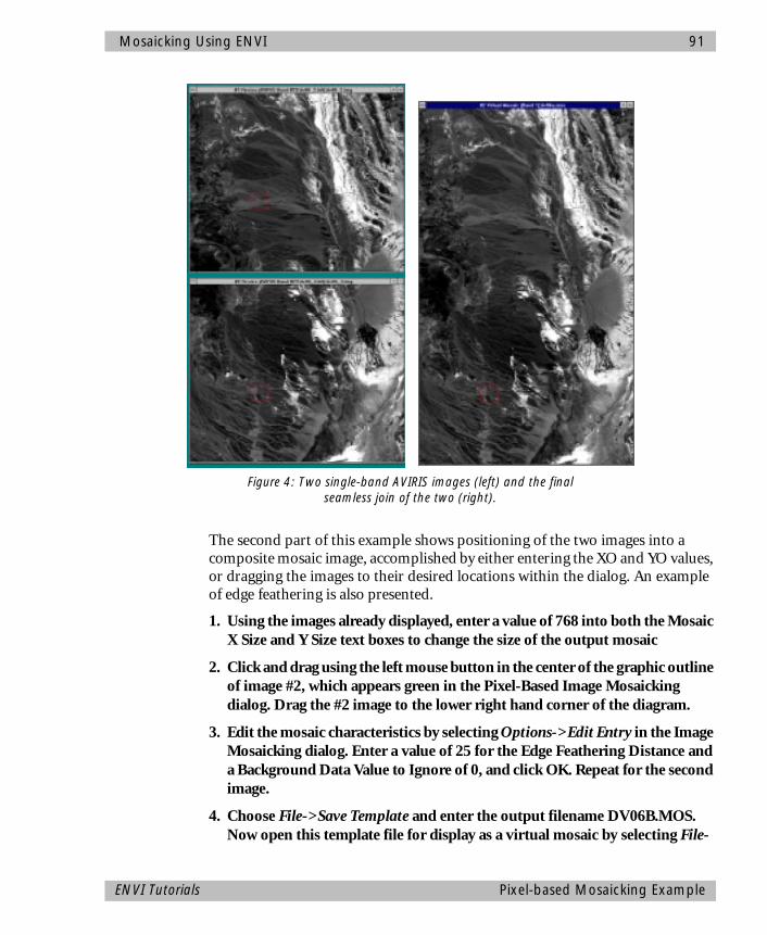
Mosaicking Using ENVI 91
The second part of this example shows positioning of the two images into a composite mosaic image, accomplished by either entering the XO and YO values, or dragging the images to their desired locations within the dialog. An example of edge feathering is also presented.
1. Using the images already displayed, enter a value of 768 into both the Mosaic X Size and Y Size text boxes to change the size of the output mosaic
2. Click and drag using the left mouse button in the center of the graphic outline of image #2, which appears green in the Pixel-Based Image Mosaicking dialog. Drag the #2 image to the lower right hand corner of the diagram.
3. Edit the mosaic characteristics by selecting Options->Edit Entry in the Image Mosaicking dialog. Enter a value of 25 for the Edge Feathering Distance and a Background Data Value to Ignore of 0, and click OK. Repeat for the second image.
4. Choose File->Save Template and enter the output filename DV06B.MOS. Now open this template file for display as a virtual mosaic by selecting File-
Figure 4: Two single-band AVIRIS images (left) and the final seamless join of the two (right).
ENVI Tutorials Pixel-based Mosaicking Example
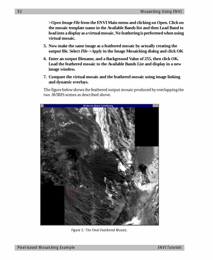
92 Mosaicking Using ENVI
>Open Image File from the ENVI Main menu and clicking on Open. Click on the mosaic template name in the Available Bands list and then Load Band to load into a display as a virtual mosaic. No feathering is performed when using virtual mosaic.
5. Now make the same image as a feathered mosaic by actually creating the output file. Select File->Apply in the Image Mosaicking dialog and click OK
6. Enter an output filename, and a Background Value of 255, then click OK. Load the feathered mosaic to the Available Bands List and display in a new image window.
7. Compare the virtual mosaic and the feathered mosaic using image linking and dynamic overlays.
The figure below shows the feathered output mosaic produced by overlapping the two AVIRIS scenes as described above.
Figure 5: The Final Feathered Mosaic.
Pixel-based Mosaicking Example ENVI Tutorials
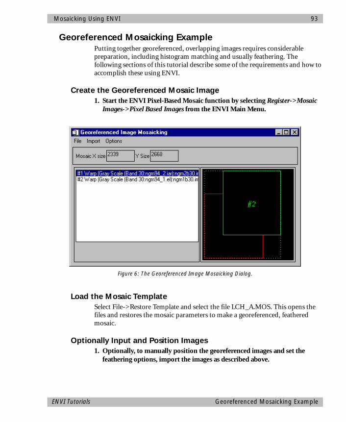
Mosaicking Using ENVI 93
Georeferenced Mosaicking ExamplePutting together georeferenced, overlapping images requires considerable preparation, including histogram matching and usually feathering. The following sections of this tutorial describe some of the requirements and how to accomplish these using ENVI.
Create the Georeferenced Mosaic Image1. Start the ENVI Pixel-Based Mosaic function by selecting Register->Mosaic
Images->Pixel Based Images from the ENVI Main Menu.
Load the Mosaic TemplateSelect File->Restore Template and select the file LCH_A.MOS. This opens the files and restores the mosaic parameters to make a georeferenced, feathered mosaic.
Optionally Input and Position Images1. Optionally, to manually position the georeferenced images and set the
feathering options, import the images as described above.
Figure 6: The Georeferenced Image Mosaicking Dialog.
ENVI Tutorials Georeferenced Mosaicking Example

94 Mosaicking Using ENVI
Images will automatically be placed in their correct geographic locations. The location and size of the georeferenced images will determine the size of the output mosaic.
View the Top Image and Cutline1. In the Available Bands List, select the file LCH_01W.IMG and display as a
grayscale by clicking on the band name and then the Load Band button at the bottom of the dialog.
2. Click the right mouse button in the Main Image Display window to toggle the Functions menu, then choose Functions->Overlays->Annotation to start the Annotation dialog.
3. Select File->Restore Annotation and choose the file LCH_01W.ANN to display the cutline used to blend the two images in this mosaic.
4. Display the second image lch_02w.img and examine the nature of the cutline with respect to this image.
View the Virtual, Non-Feathered Mosaic.1. Select File->Open File from the ENVI Main Menu and choose LCH_A.MOS
as the input file. Load this image to a new display using the Available Bands List and examine the non-feathered edge between the two images used to create the mosaic.
Create the Output Feathered Mosaic1. Select File->Apply in the Georeferenced Image Mosaicking dialog and enter
the output filename LCH_MOS.IMG and click OK to create the feathered mosaic.
2. Close the two Image Display Windows containing the individual warped images and load the mosaic image into a new display.
3. Compare the feathered mosaic to the non-feathered mosaic using image linking and dynamic overlays.
Some Additional Options in The Mosaicking dialog
• To float the pixel-based image to the top of the stack of overlapping images, click on the image desired in the list, or the mosaic diagram, and select Options->Percolate.
This option is only available for pixel-based images.
Georeferenced Mosaicking Example ENVI Tutorials
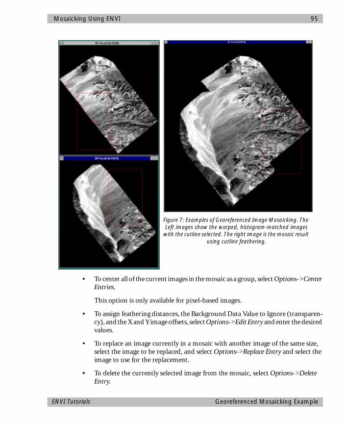
Mosaicking Using ENVI 95
• To center all of the current images in the mosaic as a group, select Options->Center Entries.
This option is only available for pixel-based images.
• To assign feathering distances, the Background Data Value to Ignore (transparen-cy), and the X and Y image offsets, select Options->Edit Entry and enter the desired values.
• To replace an image currently in a mosaic with another image of the same size, select the image to be replaced, and select Options->Replace Entry and select the image to use for the replacement.
• To delete the currently selected image from the mosaic, select Options->Delete Entry.
Figure 7: Examples of Georeferenced Image Mosaicking. The Left images show the warped, histogram-matched images
with the cutline selected. The right image is the mosaic result using cutline feathering.
ENVI Tutorials Georeferenced Mosaicking Example

96 Mosaicking Using ENVI
• To remove all images from the mosaic and clear the mosaic complete, select Options->Clear All Entries.
• To place an image as if their upper left corner has the X,Y coordinates 1,1, select Options->Do Not Use Image Offset.
Do this for images which were previously created as subsets from other larger images and which have an “image offset”. This means that the upper left corner of the image has X and Y values corresponding to its position in the original image.
• To place images in the mosaic at the location specified by its location in the original image from which it was subset, select Options->Use Image Offset.
Georeferenced Mosaicking Example ENVI Tutorials
ENVI Tutorial #5
Vector Overlay and GIS Analysis
The following topics are covered in this tutorial:
Overview of This Tutorial ........................................................................................98Data Sources and Files Used in this Tutorial .............................................................98Background - Vector Overlay and GIS Concepts in ENVI........................................100Part 1: Stand-Alone Vector GIS in ENVI .................................................................105Part 2: Combined Raster/Vector Processing Using ENVI.........................................112
97
98 Vector Overlay and GIS Analysis
Overview of This TutorialThis tutorial introduces ENVI’s vector overlay and GIS analysis capabilities using vector data from ESRI’s Maps and Data CD-ROM and a simulated 4-meter resolution Space Imaging/EOSAT multispectral dataset and associated vector data of Gonzales, California, USA. Data courtesy of ESRI and Space Imaging/EOSAT. Part 1 of this tutorial uses ESRI’s data to demonstrate stand-alone vector GIS analysis, including input of ArcView Shape Files and associated .dbf attribute files, display in vector windows, viewing/editing of attribute data, point-and-click spatial query, and math/logical query operations. Part 2 of this tutorial uses the Space Imaging/EOSAT data to demonstrate use of ENVI’s combined image display/vector overlay and analysis capabilities, including cursor tracking with attribute information, point-and-click query, and heads-up digitizing and vector layer editing. Also demonstrated are generation of new vector layers using math/logical query operations and raster-to-vector conversion of ENVI Regions of Interest (ROI) and/or classification images. Finally, the exercise demonstrates ENVI’s vector-to-raster conversion, using vector query results to generate ROIs for extraction of image statistics and area calculations. It is assumed that the user already as a basic grasp of GIS analysis concepts.
Data Sources and Files Used in this TutorialThe data used in this tutorial are provided courtesy of the Environmental Systems Research Institute Inc. and Space Imaging/EOSAT and may not be redistributed without explicit permission from those organizations.
ESRI Data and Maps Version 1 CD-ROMExample data used in Part 1 of this tutorial come from the ESRI Data and Maps Version 1 CD-ROM distributed with ARCView Version 3.0. BSC is an ESRI Business Partner and strives to maintain import/export compatibility with ESRI GIS products and data formats,
Topics Covered in This TutorialOverview of This Tutorial
Data Sources and Files Used in this Tutorial
Background - Vector Overlay and GIS Concepts in ENVI• Capabilities• ENVI Vector Files (.evf)• The Available Vectors List• Create World Boundaries• The Vector Parameters Window• ENVI Attributes
Part 1: Stand-Alone Vector GIS in ENVI• Generate USA State Boundaries• Open and Load ArcView Shape
Files to Vector Window• Zoom to Area of Interest• Edit Layer Parameters• View/Edit Attributes• Point-and-Click Query• Query Attributes• Sort Attribute and Highlight• Annotate Vector Map
Part 2: Combined Raster/Vector Processing Using ENVI• Load Data to Combined
Image/Vector Display• Track attributes with cursor• Heads-up Digitizing• Vector Layer Editing• Query Operations• ROI and Classification-to-
Vector Conversions• Vector-to-Raster Conversions• Extraction of image statistics
and polygon areas• Image-Map Output• Raster Classification to Vector
Overview of This Tutorial ENVI Tutorials
Vector Overlay and GIS Analysis 99
including ARCView Shape files and ARC/INFO export files (.e00, non-compressed).
Space Imaging EOSAT CarterraTM Agriculture Sampler DataExample images and vector data used in Part II of this tutorial are from the Space Imaging EOSAT Carterra Agriculture Sampler CD-ROM (Copyright © 1997, Space Imaging EOSAT), and are used with their explicit permission. This sample data set covers an agricultural area near Gonzales, California, USA; the north-central portion of the Palo Escrito Peak, CA USGS 7.5 minute quadrangle. The digital imagery are simulated data products designed to be similar to the space-based image data products that will be collected and distributed by Space Imaging EOSAT in early 1998. They are provided by Space Imaging EOSAT to give current and future users of digital imagery a early look at the imagery products that they will be collecting from orbit. These simulated data sets provide a reasonable example of the types of information that will be extractable from the future Space Imaging EOSAT imagery products. The imagery data sets were generated from digital image data collected by an air-borne multispectral scanner. The air-borne data were geometrically rectified, solar corrected and mosaicked at a spatial resolution simulating the future CARTERRA data products. There are, however, both radiometric and geometric differences between these data and satellite-based products planned for delivery. Please see the Carterra Sampler readm.txt file included in the SI_EOSAT subdirectory for additional information.
Required FilesYou must have the ENVI TUTORIALS & DATA CD-ROM mounted on your system to access the files used by this tutorial, or copy the files to your disk.
The files used in Part 1 of this tutorial are contained in the ESRI_GIS subdirectory of the ENVIDATA directory on the ENVI TUTORIALS & DATA CD-ROM.
Files used in Part 2 of this tutorial are contained in the SI_EOSAT subdirectory of the ENVIDATA directory on the ENVI TUTORIALS & DATA CD-ROM.
Required Vector GIS Files for Part 1CITIES.SHP (.shx, .dbf, .evf)USA Cities PointsSTATES.SHP (.shx, .dbf, .evf) USA States Polygons)
Optional Vector GIS Files for Part 1COUNTIES.SHP (.shx, .dbf,.evf) USA Counties Polygons)DRAINAGES.SHP (.shx,.dbf,.evf) USA Drainage Polygons)
ENVI Tutorials Data Sources and Files Used in this Tutorial
100 Vector Overlay and GIS Analysis
RIVER.SHP (.shx, .dbf, .evf) USA Rivers Polylines)ROADS.SHP (.shx, .dbf, .evf) USA Roads Polylines)STATES.VEC ENVI Vector TemplateALASKA.VEC ENVI Vector TemplateHAWAII.VEC ENVI Vector Template
Required Image Files for Part 20826_MS.IMG 4-meter Multispectral data0826_MS.HDR ENVI Header for AboveCAN_TMR.IMG Canon City TM dataCAN_TMR.HDR ENVI Header for AboveCAN_SAM.IMG Canon City SAM ClassificationCAN_SAM.HDR ENVI Header for AboveCAN_SV.IMG Sieved Classification (threshold=5)CAN_SV.HDR ENVI Header for AboveCAN_CLMP.IMG Clumped (5 x 5) after SieveCAN_CLMP.HDR ENVI Header for AboveCAN_TM1.ROI Canon City TM ROI #1CAN_TM2.ROI Canon City TM ROI #2
Required Vector Files for Part 2VECTORS.SHP (.shx, .dbf, .evf) Fld Outlines Polygons)
Optional Vector Files for Part 2GLORIA.EVF, (.dbf) Query Results Polygons)LANINI.EVF, (.dbf) Query Results Polygons)SHARPE.EVF, (.dbf) Query Results Polygons)
Background - Vector Overlay and GIS Concepts in ENVI
CapabilitiesENVI Version 3.0 provides extensive vector overlay and GIS analysis capabilities. These include:
• Import support for industry-standard GIS file formats including ArcView Shape files and associated .dbf attribute files, Arc/Info Interchange (uncompressed), DXF, USGS DLG and USGS STDS formats. ENVI uses an internal binary format (.evf) to maximize performance.
Background - Vector Overlay and GIS Concepts in ENVI ENVI Tutorials
Vector Overlay and GIS Analysis 101
• Vector or Image/Vector Displays: ENVI provides a stand-alone GIS plot window for displaying vector data and composing simple vector-only maps. More impor-tantly, ENVI provides vector overlays on standard ENVI displays including true vectorization of overlays in all windows, including zoom window.
• Generate world boundary vector layers including both low- and high-resolution political boundaries, coastlines, and rivers, as well as the USA state boundaries for display in vector windows or overlay on image displays.
• Heads-up (on-screen) Digitizing can be performed in either the vector or raster image window. Heads-up digitizing provides an easy means of creating new vector layers by adding polygons, lines, or points.
• Image-based and vector window-based vector editing allows users to modify individual polygons, polylines, and points in vector layers using standardized editing tools, taking full advantage of the image backdrop provided by raster images in ENVI.
• Regions-of-interest, specific image contour values, classification images and other raster processing results can easily be converted to vector format for use in GIS processing.
• Track vectors in either vector or image display windows. Display latitude/longi-tude and map coordinate information. Export map coordinates to image-to-map registration. Open a Vector Information window and display attribute informa-tion in real-time as the cursor tracks each vector.
• ENVI supports linked vectors and attribute tables with point-and-click query for both vector and raster displays. Click on a vector in the display window, and the corresponding vector and its associated information is highlighted in the attribute table. Click on an attribute in the table, and the display scrolls to and highlights the corresponding vector.
• Scroll and pan through rows and columns of data in attribute tables. Edit existing information or replace individual attributes with constant values, or with data imported from ASCII files. Add or delete attribute columns. Sort column infor-mation in either forward or reverse order. Save attribute records to ASCII format.
• Query vector GIS database information directly to generate new layers of selected information with attributes. Allows GIS analysis of layers using simple mathemat-ical functions and logical operators to produce new information and layers. In keeping with established ENVI processing paradigms, results can either be held in memory, or saved to file for later access.
ENVI Tutorials Background - Vector Overlay and GIS Concepts in ENVI
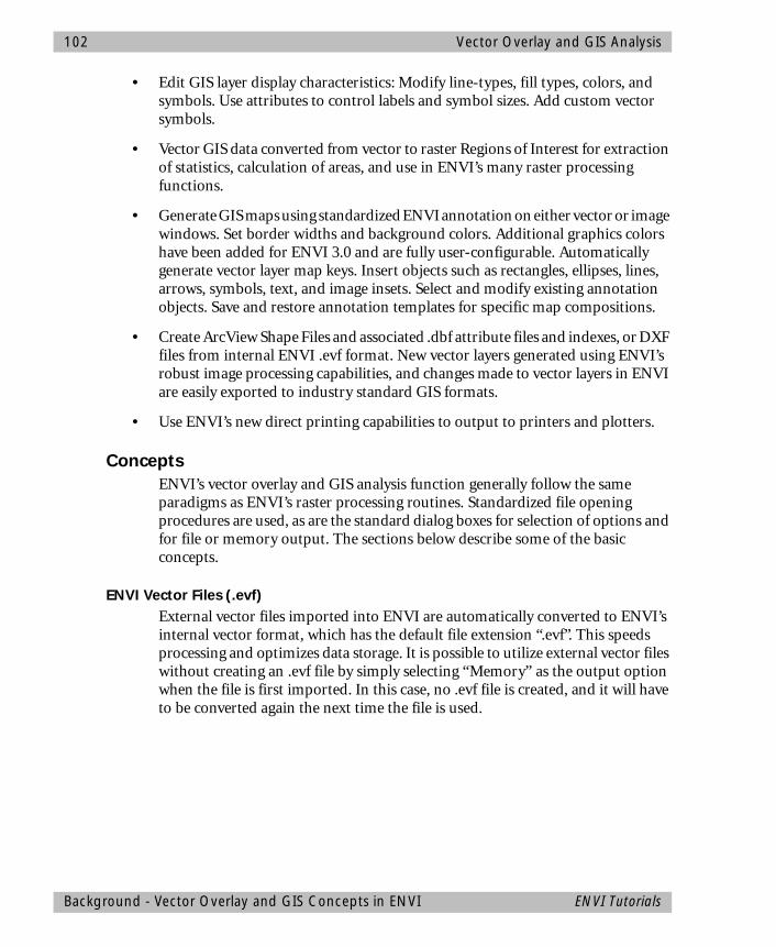
102 Vector Overlay and GIS Analysis
• Edit GIS layer display characteristics: Modify line-types, fill types, colors, and symbols. Use attributes to control labels and symbol sizes. Add custom vector symbols.
• Vector GIS data converted from vector to raster Regions of Interest for extraction of statistics, calculation of areas, and use in ENVI’s many raster processing functions.
• Generate GIS maps using standardized ENVI annotation on either vector or image windows. Set border widths and background colors. Additional graphics colors have been added for ENVI 3.0 and are fully user-configurable. Automatically generate vector layer map keys. Insert objects such as rectangles, ellipses, lines, arrows, symbols, text, and image insets. Select and modify existing annotation objects. Save and restore annotation templates for specific map compositions.
• Create ArcView Shape Files and associated .dbf attribute files and indexes, or DXF files from internal ENVI .evf format. New vector layers generated using ENVI’s robust image processing capabilities, and changes made to vector layers in ENVI are easily exported to industry standard GIS formats.
• Use ENVI’s new direct printing capabilities to output to printers and plotters.
ConceptsENVI’s vector overlay and GIS analysis function generally follow the same paradigms as ENVI’s raster processing routines. Standardized file opening procedures are used, as are the standard dialog boxes for selection of options and for file or memory output. The sections below describe some of the basic concepts.
ENVI Vector Files (.evf)External vector files imported into ENVI are automatically converted to ENVI’s internal vector format, which has the default file extension “.evf”. This speeds processing and optimizes data storage. It is possible to utilize external vector files without creating an .evf file by simply selecting “Memory” as the output option when the file is first imported. In this case, no .evf file is created, and it will have to be converted again the next time the file is used.
Background - Vector Overlay and GIS Concepts in ENVI ENVI Tutorials
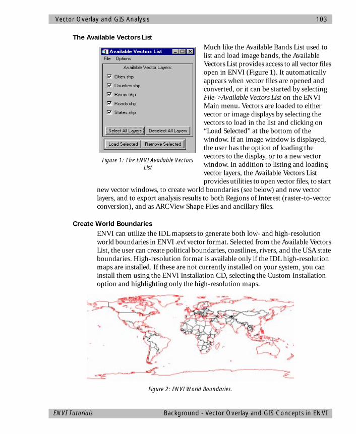
Vector Overlay and GIS Analysis 103
The Available Vectors ListMuch like the Available Bands List used to list and load image bands, the Available Vectors List provides access to all vector files open in ENVI (Figure 1). It automatically appears when vector files are opened and converted, or it can be started by selecting File->Available Vectors List on the ENVI Main menu. Vectors are loaded to either vector or image displays by selecting the vectors to load in the list and clicking on “Load Selected” at the bottom of the window. If an image window is displayed, the user has the option of loading the vectors to the display, or to a new vector window. In addition to listing and loading vector layers, the Available Vectors List provides utilities to open vector files, to start
new vector windows, to create world boundaries (see below) and new vector layers, and to export analysis results to both Regions of Interest (raster-to-vector conversion), and as ARCView Shape Files and ancillary files.
Create World BoundariesENVI can utilize the IDL mapsets to generate both low- and high-resolution world boundaries in ENVI .evf vector format. Selected from the Available Vectors List, the user can create political boundaries, coastlines, rivers, and the USA state boundaries. High-resolution format is available only if the IDL high-resolution maps are installed. If these are not currently installed on your system, you can install them using the ENVI Installation CD, selecting the Custom Installation option and highlighting only the high-resolution maps.
Figure 1: The ENVI Available Vectors List
Figure 2: ENVI World Boundaries.
ENVI Tutorials Background - Vector Overlay and GIS Concepts in ENVI
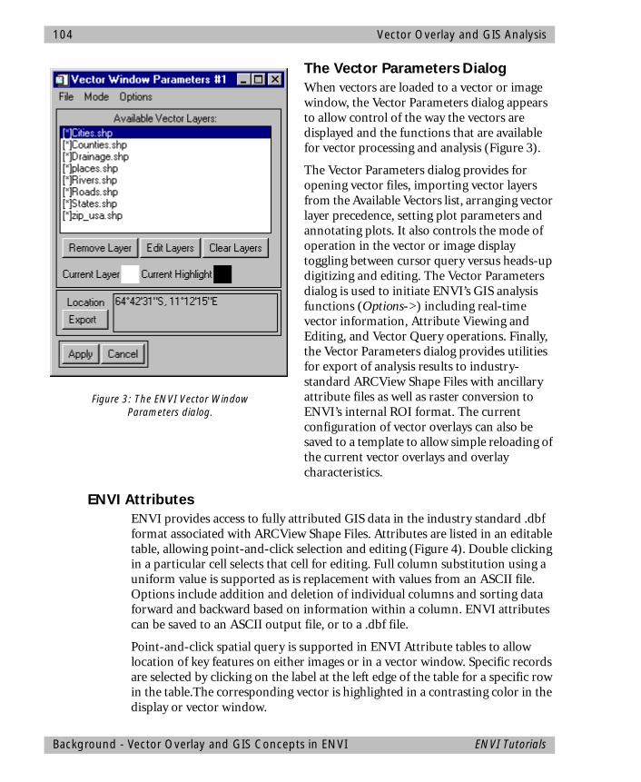
104 Vector Overlay and GIS Analysis
The Vector Parameters DialogWhen vectors are loaded to a vector or image window, the Vector Parameters dialog appears to allow control of the way the vectors are displayed and the functions that are available for vector processing and analysis (Figure 3).
The Vector Parameters dialog provides for opening vector files, importing vector layers from the Available Vectors list, arranging vector layer precedence, setting plot parameters and annotating plots. It also controls the mode of operation in the vector or image display toggling between cursor query versus heads-up digitizing and editing. The Vector Parameters dialog is used to initiate ENVI’s GIS analysis functions (Options->) including real-time vector information, Attribute Viewing and Editing, and Vector Query operations. Finally, the Vector Parameters dialog provides utilities for export of analysis results to industry-standard ARCView Shape Files with ancillary attribute files as well as raster conversion to ENVI’s internal ROI format. The current configuration of vector overlays can also be saved to a template to allow simple reloading of the current vector overlays and overlay characteristics.
ENVI AttributesENVI provides access to fully attributed GIS data in the industry standard .dbf format associated with ARCView Shape Files. Attributes are listed in an editable table, allowing point-and-click selection and editing (Figure 4). Double clicking in a particular cell selects that cell for editing. Full column substitution using a uniform value is supported as is replacement with values from an ASCII file. Options include addition and deletion of individual columns and sorting data forward and backward based on information within a column. ENVI attributes can be saved to an ASCII output file, or to a .dbf file.
Point-and-click spatial query is supported in ENVI Attribute tables to allow location of key features on either images or in a vector window. Specific records are selected by clicking on the label at the left edge of the table for a specific row in the table.The corresponding vector is highlighted in a contrasting color in the display or vector window.
Figure 3: The ENVI Vector Window Parameters dialog.
Background - Vector Overlay and GIS Concepts in ENVI ENVI Tutorials
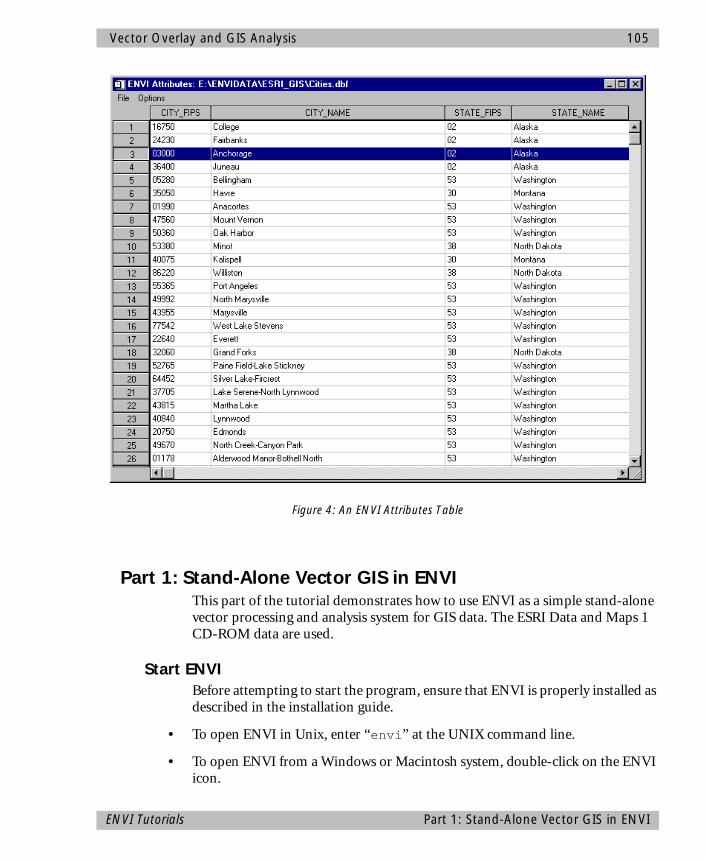
Vector Overlay and GIS Analysis 105
Part 1: Stand-Alone Vector GIS in ENVIThis part of the tutorial demonstrates how to use ENVI as a simple stand-alone vector processing and analysis system for GIS data. The ESRI Data and Maps 1 CD-ROM data are used.
Start ENVIBefore attempting to start the program, ensure that ENVI is properly installed as described in the installation guide.
• To open ENVI in Unix, enter “envi” at the UNIX command line.
• To open ENVI from a Windows or Macintosh system, double-click on the ENVI icon.
Figure 4: An ENVI Attributes Table
ENVI Tutorials Part 1: Stand-Alone Vector GIS in ENVI

106 Vector Overlay and GIS Analysis
The ENVI Main Menu appears when the program has successfully loaded and executed.
Open an ArcView Vector File (Shape File)To open a vector file:
1. Select File -> Open Vector File->ArcView Shape File
Note that on some platforms you must hold the left mouse button down to display the submenus from the Main Menu.
An Enter Input Data File file selection dialog appears.
2. Navigate to the ESRI_GIS subdirectory of the ENVIDATA directory on the ENVI TUTORIALS & DATA CD-ROM just as you would in any other application and select the file CITIES.SHP from the list and click “OPEN”.
The Import ArcView Shape File Parameters dialog will appear on your screen. This list allows you to select the file or memory output, enter the output filename for the ENVI .evf file, and choose the output projection for the data.
3. Select Memory Output and choose the default values by simply clicking on “OK”. A status window will appear indicating the number of vector vertices being read and the Available Vectors List will appear when the data have been converted.
4. Alternatively, use Select File->Open Vector File->ENVI Vector File (.evf) to open the existing .EVF files.
5. Select the vector layer to be loaded by clicking in the checkbox to the left of the CITIES.SHP entry in the Available Vectors List. Click on Load Selected to start a new vector window and the Vector Window Parameters dialog.
6. Click on Apply in this dialog to load CITIES.SHP into the vector display.
The cities of the United States will be plotted in the vector display.
Work with Vector Point data1. Click using the left mouse button in the vector window and hold down the
button and drag the cursor around the vector window to read latitude and longitude in the Vector Window Parameters dialog.
2. Zoom in on just the contiguous 48 states by positioning the cursor just to the northwest of cities marked in the state of Washington and clicking and dragging using the middle mouse button to define a box covering the desired region.
Part 1: Stand-Alone Vector GIS in ENVI ENVI Tutorials

Vector Overlay and GIS Analysis 107
Releasing the mouse button defines the lower right corner of the area selected and causes the display to be zoomed in on just that area. Multiple levels of zoom are possible. Clicking the middle mouse button anywhere in the display zooms out one level.
3. Change the symbol used to mark the cities, by clicking on Edit Layers in the Vector Window Parameters dialog and selecting “Flag” from the pulldown Symbol menu. clicking on OK at the bottom of the dialog, then Apply at the bottom of the Vector Window Parameters dialog.
(You can add your own symbols by defining them in the file usersym.txt in the ENVI30/Menu directory of your ENVI installation.)
4. Also experiment with changing other vector display characteristics by selecting Edit Layers and changing the desired characteristics (color, symbol, size) in the Edit Vector Layers dialog.
Create the USA state boundaries using IDL mapsets1. Select Options->Create World Boundaries in the Available Vectors List.
The Create Boundaries dialog appears.
2. Click in the check box next to USA States, select the Memory radio button, and click on OK to create the USA Boundaries and load to the Available Vectors List.
3. Click in the textbox next to USA States and then on the Load Selected button a the bottom of the Available Vectors List and choose Vector Window #1 in the Load Vector dialog as the location to load the vector. Click Apply in the Vector Parameters dialog to plot the vectors.
Both the cities previously selected and the state boundaries will be displayed in the vector window. The state boundaries in this case are polylines, that is, they are not true polygons (because of the way the were digitized and stored).
4. Click on USA States in the Vector Parameters dialog and choose Edit Layers to change parameters for the state boundaries, including color, line style, and thickness. Remember to click on the Apply button in the Vector Parameters dialog to plot the changes.
5. Clear the state boundaries by clicking on the Available Vector Layer USA States in the Vector Window Parameters dialog and then on Remove Layer.
Work with Vector Polygon Data6. Select File->Open Vector File->ArcView Shape File from the menu in the
Vector Parameters dialog. Choose STATES.SHP and click on Open. Select
ENVI Tutorials Part 1: Stand-Alone Vector GIS in ENVI
108 Vector Overlay and GIS Analysis
Memory Output and choose the default values by simply clicking on “OK”. A status window will appear indicating the number of vector vertices being read and the Available Vectors List will appear when the data have been converted.
7. Alternatively, use Select File->Open Vector File->ENVI Vector File (.evf) to open the existing .EVF files.
This loads STATES.SHP into the Available Vectors List.
8. Make sure that the USA States boundaries previously used are deselected in the Available Vectors List (no check mark in the box) and select STATES.SHP by clicking in the check box next to the name. Click on Load Selected and then Choose Vector Window #1 in the Load Vector dialog.
9. Select STATES.SHP as the Available Vector Layer in the Vector Window Parameters dialog and click on Edit Layers and change the color to green and the fill to “line”. Click on OK, then Apply in the Vector Window Parameters dialog to redisplay the vectors with changes applied.
10.Change the vector layer precedence by selecting Options->Arrange Layer Order, clicking on one of the vector layer names in the Vector Layer Ordering dialog and dragging it to the desired position in the stack.
Get Vector Information and Attributes1. Select CITIES.SHP as the Available Vector Layer in the Vector Window
Parameters dialog and choose Options->Vector Information to start the Vector Information window, listing attributes for each data point. Click and drag using the left mouse button on the city flags in the Vector window to see the basic attribute information from the ArcView .dbf attribute file.
2. Find your hometown or the nearest city by examining the CITY_NAME attribute in the Vector Information dialog and then find the latitude and longitude by looking in the Vector Window Parameters dialog.
View Attributes and Point-and-Click Query1. Make sure that CITIES.SHP is selected and choose Options->View/Edit
Attributes in the Vector Window Parameters dialog to start an ENVI Attributes table.
This is a fully editable table of the attributes for the selected layer.
2. Click in the left column to do a spatial query on the selected city. The corresponding city flag will be highlighted in the vector window. If desired, zoom in on the specific city selected by clicking and dragging a box around
Part 1: Stand-Alone Vector GIS in ENVI ENVI Tutorials
Vector Overlay and GIS Analysis 109
the highlighted city using the left mouse button. Zoom back out by clicking the middle mouse button in the window.
3. Verify that you have selected the correct city by clicking with the left mouse button on the city flag and observing the attributes in the Vector Information window.
4. Edit the elevation value for the selected city by scrolling the ENVI Attribute window to the right until you can view the Elevation attribute, and double clicking with the left mouse button in the corresponding elevation table cell. Enter a new value and press the return (enter) key to change the value.
5. Now do a map-based query by clicking on a city flag and observing that the corresponding record is highlighted in the ENVI Attributes table. Drag the vector cursor around the country from city flag to city flag and note how the ENVI Attribute table scrolls to follow the selected cities.
Query Attributes1. Make sure that CITIES.SHP is selected in the Vector Window Parameters
dialog and select Options->Query Attributes. Enter a name for the layer to be generated in the Query Layer Name text box (use “Where State==California”.) Click on the Start button to begin the query.
The Query Condition dialog will appear
2. Click on the left button in the dialog (which starts with the “CITY_FIPS” attribute displayed), pulldown and select “STATE_NAME”. Now choose the operator “==” from the list of options on the pulldown initially marked “<“in the center of the dialog. Finally, enter the string “California” (be sure to match case) in the String Value text box.
3. When the Layer Attribute Query dialog appears, click the Memory radio button and the OK to begin the query.
ENVI creates a new vector layer with associated .dbf file based on the results of the query and lists the new layer in the Vector Window Parameters and the Available Vectors dialogs.
4. Click Apply to highlight the selected vectors in the vector window in a new color.
5. Zoom in on the selected vectors using the middle mouse button to drag and draw an outlining box around the state of California.
6. Open the new .dbf attribute file by clicking on the new layer name in the Vector Window Parameters dialog and then selecting Options->View/Edit
ENVI Tutorials Part 1: Stand-Alone Vector GIS in ENVI
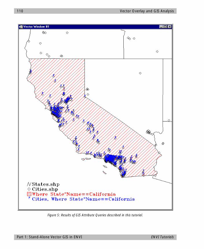
110 Vector Overlay and GIS Analysis
Figure 5: Results of GIS Attribute Queries described in this tutorial.
Part 1: Stand-Alone Vector GIS in ENVI ENVI Tutorials

Vector Overlay and GIS Analysis 111
Attributes. When the ENVI Attribute table appears, try some point-and-click query operations as described above to see the association between the selected cities, their locations in the vector window, and the attributes.
The easiest way to find a specific city is to sort the attributes and then click on the city name.
7. Click at the top of the CITY_NAME column in the ENVI Attribute table to highlight that complete set of attributes. Select Options->Sort by selected column forward to sort the column alphabetically. Now scroll down the column and click on “Sacramento” to highlight the location of the capital of California in a different color in the vector window.
Annotate Map Key in Vector WindowENVI provides tools to generate a basic vector map from the ENVI Vector window. These are essentially the same as the annotation tools used for ENVI image and plot annotation, so no details are covered here. The description below demonstrates how to put a map key in the annotation window.
1. Select Options->Annotate Plot in the Vector Windows Parameters dialog to begin. In the Annotation dialog, select Object->Map Key to automatically create a map key for the vector layers. Click the left mouse button in the Vector Display window to place and move the annotation. The characteristics of the key are controlled by clicking on Edit Map Key Items and selecting the desired changes. Return to placing the annotation by clicking OK. Click the right mouse button in the Vector window to finalize placement of the map key. All annotation in the vector window follows the same paradigms as annotation in ENVI display windows. See the descriptions of Annotation in the ENVI User’s Guide for additional details.
Close the windows and all files1. Click on Select All Layers in the Available Vectors List then on Remove
Selected. Close the Available Vectors List by selecting File->Cancel.
2. Close the vector window and all associate dialogs and tables by selecting File->Cancel in the Vector Window Parameters dialog.
This concludes Part 1 of the exercise.
ENVI Tutorials Part 1: Stand-Alone Vector GIS in ENVI
112 Vector Overlay and GIS Analysis
Part 2: Combined Raster/Vector Processing Using ENVIThis section of the tutorial demonstrates how to use Vector Overlays and GIS data and attributes within ENVI in combination with raster images. Data from Space Imaging EOSAT are used.
Load Image Data to Combined Image/Vector DisplayTo open an image file to use as a backdrop for vector layers:
1. Select File->Open Image File from the ENVI Main menu.
Note that on some platforms you must hold the left mouse button down to display the submenus from the Main Menu.
An Enter Input Data File selection dialog appears.
2. Navigate to the SI_EOSAT subdirectory of the ENVIDATA directory on the ENVI TUTORIALS & DATA CD-ROM just as you would in any other application and select the file 0826_MS.IMG from the list and click “OPEN”.
The Available Bands List will appear with four spectral bands listed. These data are a simulated 4-meter Space Imaging EOSAT multispectral dataset with spectral band coverage similar to the first 4 spectral bands of Landsat Thematic Mapper data.
3. The bands to load into a color composite have already been selected using ENVI 3.0’s default bands option in the ENVI header file. Click on Load RGB to load a true-color image into a new image display window.
Open a Vector Layer and Load to Image Display1. Click the right mouse button in the image display to toggle the Functions
menu and choose Functions->Overlays->Vector Layers to start the Display Vector Parameters dialog.
2. Select File->Open Vector File->ArcView Shape File from the menu bar in the Display Vector Parameters dialog, select the file VECTORS.SHP from the list and click “OPEN”.
Note You could also have used the File->Open Vector File->ArcView Shape File methods used above from the ENVI main menu to accomplish the same thing. ENVI provides several methods of accessing the vector overlays. Users can choose the method most consistent with their applications and approach to processing.
The Import ArcView Shape File Parameters dialog will appear on your screen. As described above, this list allows you to select the file or memory output, enter the
Part 2: Combined Raster/Vector Processing Using ENVI ENVI Tutorials
Vector Overlay and GIS Analysis 113
output filename for the ENVI .evf file, and choose the output projection for the data.
3. In the Import ArcView Shape File Parameters dialog, click on State Plane (NAD 83) as the Output Projection and select #404 California IV as the Zone by clicking on the Zone button, choosing zone #404 from the list in the Select State Plane Zone dialog and clicking OK. Select memory output and click on OK in the Import ArcView Shape File Parameters dialog to complete the projection selection.
4. Alternatively, use Select File->Open Vector File->ENVI Vector File (.evf) to open the existing .EVF files.
A status window will appear indicating the number of vector vertices being read. When the data have been converted (.shp) or inported (.evf), the Available Vectors List will appear listing the VECTOR layer and the layer will be automatically loaded into the Display Vector Parameters dialog.
5. Click on Apply in the Display Vector Parameters dialog to load the vectors into the image display as an overlay on the displayed image.
6. Choose Edit Layers and change the color of the vectors to red, click OK, then Apply to reload the modified vectors onto the image.
Track attributes with cursor1. Select Options->Vector Information to start the Vector Information window
and click and drag using the left mouse button in the image to view the attribute information for the vectors. Also observe the latitude and longitude listed in the Display Vector Parameters dialog. Select the Scroll and Zoom radio buttons in the Display Vector Parameters dialog to allow vector tracking in the corresponding window. Select the Off radio button to allow normal scrolling in the Scroll and Main Windows and zooming in the Zoom window. Try different zoom factors in the Zoom window to assess the accuracy of the vectors.
2. Select Options->View/Edit Attributes in the Display Vector Parameters dialog to load the ENVI Attribute table for these data. Utilize point-and-click query as described for the vector-only case above by clicking in the left (numbered) column of the attribute table to find and highlight specific polygons on the image.
Heads-up (on-screen) DigitizingENVI provides vector editing routines for adding your own vectors to an existing vector layer or for creating new vector layers. These function in a similar fashion
ENVI Tutorials Part 2: Combined Raster/Vector Processing Using ENVI

114 Vector Overlay and GIS Analysis
to ENVI’s annotation polygons, polylines, and points. ENVI heads-up vector digitizing allows creation of new polygons, polylines, points, rectangles, and ellipses.
To add new objects to a vector layer choose the layer name first from the list in the Display Vector Parameters dialog. Then select Mode->Add New Object->Object, where Object is one of the object types described above. For the purposes of this exercise, we will create a new polygon layer
1. To create a new layer, select Options->Create New Layer. Enter a name for the layer in the New Vector Layer Parameters dialog, choose the Memory radio button, and click OK.
2. Click on the new layer name in the Display Vector Parameters dialog and a new .dbf file is initialized. Choose Mode->Add New Polygon to begin adding polygons to the layer.
3. In the image display (Scroll or Zoom if selected using the radio button in the Display Vector Parameters dialog), click the left mouse button to draw polygon segments. Click the middle mouse button to erase polygon segments. Click the right mouse button to close the polygon, and a second time to accept the polygon. Polylines (line segments) are added the same way, while for points, clicking the left mouse button places the point, the middle deletes it, and the right mouse button finalizes the placement.
4. Draw a few polygons using field outlines on the image as quides.
5. To add Attributes to the newly created polygons, select Options->Add Attributes in the Display Vector Parameters dialog. Enter a name (Enter Field ID) for the attribute in the Name field in the Attribute Initialization dialog and choose the Type for the parameter (choose Character for this first one). Click on the Add Field button at the bottom of the dialog and enter a second attribute called “Field Area” in the Name field and change the Type to Numeric. Click OK to create the Attribute Table.
6. Now edit the Attribute table as previously described. Double click on a field to make changes, enter the value, and press the return (enter) key. Use point-and-click query to see which attributes are associated with which fields.
7. Close the Attribute table by selecting File->Cancel from the menu bar at the top of the table.
Part 2: Combined Raster/Vector Processing Using ENVI ENVI Tutorials
Vector Overlay and GIS Analysis 115
Edit Vector Layers1. In the Display Vector Parameters dialog, click on the new vector layer you
created and select Mode->Edit Existing Vectors. Click using the left mouse button on one of the polygons you created previously.
The polygon will be highlighted and the nodes of the polygon will be marked with a diamond.
2. You can delete the entire polygon by selecting Mode->Delete Vector in the Display Vector Parameters dialog.
3. You can modify the vector by clicking on one of the markers with your left mouse button and dragging to a new location. The middle mouse button exits the editing function without making any changes. Clicking the right mouse button finalizes the changes and redraws the polygon.
4. To finish up this section, delete any new layers you have made by selecting, those layers in the Available Vectors List and clicking on Remove Selected. Do not remove the VECTORS.SHP layer.
Query Operations1. Choose the VECTORS.SHP layer in the Display Vector Parameters dialog by
clicking on the layer name. Select Options->View/Edit Attributes to start an ENVI Attributes table. Examine the ‘RANCH” attribute and note the predominance of three owners “gloria”, “lanini”, and ‘sharpe”. Close the attribute table by selecting File->Cancel.
2. Select Options->Query Attributes in the Display Vector Parameters dialog. Enter the Query Layer Name “Gloria Ranch” in the Layer Attribute dialog and click on the Start button. Choose RANCH from the pulldown button initially marked “AREA” set the condition to “==”, and enter “gloria” for the string value (be sure to match the case seen in the Attribute Table). Click on OK. Select the Memory radio button in the Layer Attribute Query dialog and click OK again.
The new layer generated by the query is listed in the Display Vector Parameters dialog.
3. Click on the layer name in the dialog and then on the Edit Layer button to change layer parameters. Choose Line for the fill type and then click OK. Click Apply in the Display Vector Parameters dialog.
The Gloria Ranch holdings are highlighted as a new layer.
ENVI Tutorials Part 2: Combined Raster/Vector Processing Using ENVI
116 Vector Overlay and GIS Analysis
4. Examine the attributes for this layer by selecting the layer name in the Display Vector Parameters dialog and choosing Options->View/Edit Attributes. Examine the query results.
5. Close the attribute table and repeat the query for the lanini and sharp ranches, highlighting each in a different color or pattern.
6. Try other queries on combinations of attributes by choosing one of the logical operators in the Layer Attribute Query dialog.
Vector-to-Raster ConversionsENVI provides several important links between vector analysis and raster image processing. This portion of the exercise describes how to take vector processing results, create Regions of Interest for use on the images, and extract region statistics and polygon area.
1. To create Regions of Interest (ROI) for use with ENVI raster processing, click on the name of the layer to be exported to ROI. Select File->Export to ROI in the Display Vector Parameters dialog. Do this for several of the layers you created using the Query Operations above.
The layers will be listed in the Region of Interest Controls dialog.
2. Click on the ROI name in the ROI Controls dialog and select Options->Report Areas of Regions->Meters2 to generate a report of the area of the selected region.
3. Click on the ROI name in the ROI Controls dialog and click on the Stats button at the bottom of the dialog to get the image statistics for the gloria ranch polygons in the multispectral data. Try the same thing for the other Queries you generated in the vector analysis and compare the areas and statistics.
Now that these vector polygons are ENVI ROIs, you can use the power of all of ENVI’s raster processing capabilities to analyze the image data with respect to the ROIs. This includes such activities as masking, statistics, contrast stretching, and supervised classification.
Image-Map OutputENVI provides tools to generate image maps from the combined raster/vector data in the ENVI Main Image Display window. These are essentially the same as the annotation tools used for ENVI image and plot annotation, so no details are covered here. The description below demonstrates how to put a map key in the Main Image display window.
Part 2: Combined Raster/Vector Processing Using ENVI ENVI Tutorials
Vector Overlay and GIS Analysis 117
1. Generate a map-output image with a vector key using ENVI’s image-map composition capabilities. Click the right mouse button in the Main Image Display to activate Functions menu and select Functions->Overlays->Annotation.
2. Select Object->Map Key in the Annotation Map Key dialog to automatically create a map key for the vector layers. Click the left mouse button in the Main Image Display window to place and move the annotation. The characteristics of the key are controlled by clicking on Edit Map Key Items and selecting the desired changes. Return to placing the annotation by clicking OK. Click the right mouse button in the Vector window to finalize placement of the map key. All annotation in the vector window follows the same paradigms as annotation in ENVI display windows. See the descriptions of Annotation in the ENVI User’s Guide for additional detail.
Close the windows and all files1. Click on Select All Layers in the Available Vectors List then on Remove
Selected. Close the Available Vectors List by selecting File->Cancel.
2. Close the image window and all associated dialogs and tables by selecting File->Close All Files from the ENVI main menu.
Raster to Vector ConversionsENVI can also easily convert raster processing results for use in ENVI vector processing and analysis, as well as for export to external GIS systems such as ArcView and ArcInfo. The last part of this tutorial illustrates the export of raster information to vector GIS.
Export ROI to Vector LayerRegions of Interest defined using any of ENVI’s standard methods can be exported to become one or more vector layers
Load Image Data to Image DisplayOpen an image file to use as background for ROI definition and export to vector:
1. Select File->Open Image File from the ENVI Main menu.
Note that on some platforms you must hold the left mouse button down to display the submenus from the Main Menu.
An Enter Input Data File file selection dialog appears.
ENVI Tutorials Part 2: Combined Raster/Vector Processing Using ENVI
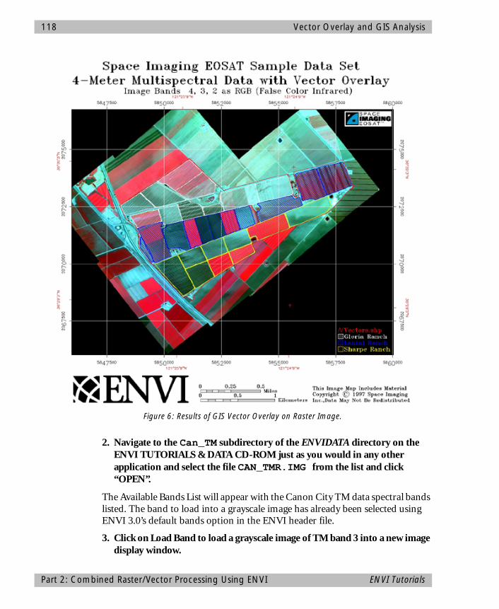
118 Vector Overlay and GIS Analysis
2. Navigate to the Can_TM subdirectory of the ENVIDATA directory on the ENVI TUTORIALS & DATA CD-ROM just as you would in any other application and select the file CAN_TMR.IMG from the list and click “OPEN”.
The Available Bands List will appear with the Canon City TM data spectral bands listed. The band to load into a grayscale image has already been selected using ENVI 3.0’s default bands option in the ENVI header file.
3. Click on Load Band to load a grayscale image of TM band 3 into a new image display window.
Figure 6: Results of GIS Vector Overlay on Raster Image.
Part 2: Combined Raster/Vector Processing Using ENVI ENVI Tutorials

Vector Overlay and GIS Analysis 119
Load Predefined ROIsSome Regions of Interest have been predefined using ENVI’s interactive ROI definition tools.
4. Click the right mouse button in the Main Image Display window to toggle the Functions menu and choose Functions->Region of Interest->Define Region of Interest to start the Region of Interest Control dialog. Select File->Restore ROIs in the ROI Controls dialog and select the ROI file CAN_TM1.ROI and click Open.
The predefined ROI will be loaded into the ROI Controls dialog and plotted on the image.
5. Repeat the above step for the file CAN_TM2.ROI.
The result is two ROIs overlain on the TM Band 3 data.
Convert ROIs to Vector6. To convert these ROIs to vector polygons, select File->Export ROI to EVF in
the ROI Controls dialog. The Export Regions to EVF dialog appears. Choose one of the regions by clicking in the check box to the left of the Region name. Choose the “All points as one record” radio button option, enter a Layer Name in the appropriate text box, click on Memory, and then OK to convert the first ROI and import to the Available Vectors List. Repeat the procedure for the second ROI.
7. In the Available Vectors List, click on Select All Layers, then the Load Selected button. Select New Vector Display in the Load Vector dialog to start a new vector window and load the new vector polygons into the Vector Window Parameters dialog. Click Apply to load the polygons. Choose Options->Add Attributes to add attributes to the polygons. These can now be used in Query and GIS analysis with other vector data or exported to ArcView Shape Files by selecting File->Export Layer to ArcView in the Vector Window Parameters dialog.
Close the windows and all files1. Click on Select All Layers in the Available Vectors List then on Remove
Selected. Close the Available Vectors List by selecting File->Cancel.
2. Close the Vector display window by clicking on File->Cancel in the Vector Window Parameters dialog.
3. Close the image window and all associated dialogs and tables by selecting File->Close All Files from the ENVI main menu.
ENVI Tutorials Part 2: Combined Raster/Vector Processing Using ENVI

120 Vector Overlay and GIS Analysis
Export Classification Image to Vector PolygonsClasses defined using any of ENVI’s standard classification methods can be exported to become one or more vector layers. ENVI also allows selection of individual image brightness levels for export as a vector layer.
Load a Classification Image to Image DisplayOpen an image file to use as background for ROI definition and export to vector:
1. Select File->Open Image File from the ENVI Main menu.
Note that on some platforms you must hold the left mouse button down to display the submenus from the Main Menu.
An Enter Input Data File file selection dialog appears.
2. Navigate to the Can_TM subdirectory of the ENVIDATA directory on the ENVI TUTORIALS & DATA CD-ROM just as you would in any other application and select the file CAN_PCLS.IMG from the list and click “OPEN”.
This is a parallelepiped classification of the Canon City TM data with 3 classes.
3. The Classification image will appear in the Available Bands List. Load this image into a grayscale image by clicking on the band name, and then on Load Band.
Generalize the classification image. To conduct successful raster-to-vector conversions, it is usually necessary to generalize the results of raster processing. If you don’t do this, you end up with vector polygons around individual pixels and small groups of pixels.
1. To demonstrate the results of generalization of the classification image, load and display the results of a 5 pixel sieve operation followed by a 5 x 5 clump operation. First display CAN_SV.IMG, the sieve results. Next display CAN_CLMP.IMG, the clump results.
2. Convert the generalized classification image to vector polygons. Select Classification->Post Classification->Classes to Vector Layers. Choose the CAN_CLMP.IMG classification for processing by clicking on the image name and then the OK button in the Raster to Vector Input Band dialog.
Create the Vector Polygons1. Select Region #1 and Region #2 by clicking in the check boxes next to the
region descriptions. Select memory execution and click OK. A status dialog
Part 2: Combined Raster/Vector Processing Using ENVI ENVI Tutorials
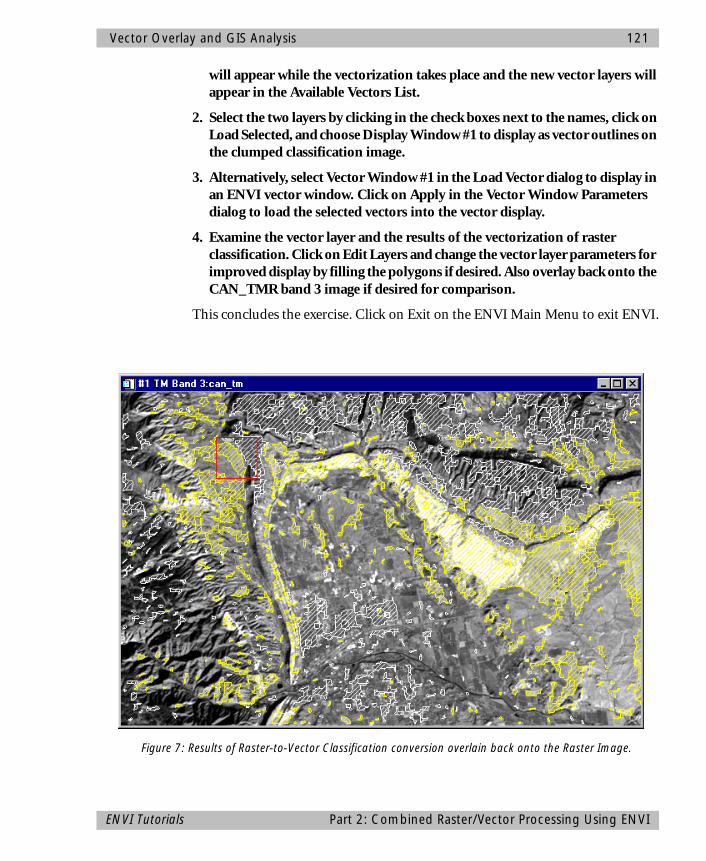
Vector Overlay and GIS Analysis 121
will appear while the vectorization takes place and the new vector layers will appear in the Available Vectors List.
2. Select the two layers by clicking in the check boxes next to the names, click on Load Selected, and choose Display Window #1 to display as vector outlines on the clumped classification image.
3. Alternatively, select Vector Window #1 in the Load Vector dialog to display in an ENVI vector window. Click on Apply in the Vector Window Parameters dialog to load the selected vectors into the vector display.
4. Examine the vector layer and the results of the vectorization of raster classification. Click on Edit Layers and change the vector layer parameters for improved display by filling the polygons if desired. Also overlay back onto the CAN_TMR band 3 image if desired for comparison.
This concludes the exercise. Click on Exit on the ENVI Main Menu to exit ENVI.
Figure 7: Results of Raster-to-Vector Classification conversion overlain back onto the Raster Image.
ENVI Tutorials Part 2: Combined Raster/Vector Processing Using ENVI

122 Vector Overlay and GIS Analysis
Part 2: Combined Raster/Vector Processing Using ENVI ENVI Tutorials
ENVI Tutorial #6
Map Composition Using ENVI
The following topics are covered in this tutorial:
Overview of This Tutorial ......................................................................................124Files Used in this Tutorial .......................................................................................124Background - Map Composition in ENVI ...............................................................124Getting Started .....................................................................................................124Image Display and Map Layout.............................................................................127
123
124 Map Composition Using ENVI
Overview of This TutorialThis tutorial is designed to give you a working knowledge of ENVI’s map composition capabilities. For additional information please see the ENVI User’s Guide or the ENVI On-Line Help.
Files Used in this TutorialYou must have the ENVI TUTORIALS & DATA CD-ROM mounted on your system to access the files used bythis tutorial, or copy the files to your disk.
The files used in this tutorial are contained in theYS_TMSUB subdirectory of the ENVIDATA directory onthe ENVI TUTORIALS & DATA CD-ROM.
Required FilesThe files listed below are required to run this exercise.
YSRATIO.IMG Yellowstone National Park TM Ratio Subset Image
YSRATIO.HDR ENVI Header for Above
YSRATIO.ANN Saved Annotation Result for Above
YSRATIO.GRD Saved Grid Parameters for Above
YS_LOC.GIF Location Image for Above
Background - Map Composition in ENVIMap composition requires that the user be able to easily and quickly go from an image to an image-based map by interactively inserting the key map components. Map composition consists of defining the map extent; positioning the image within the extent using borders; adding pixel, map coordinate, and/or geographic (latitude/longitude) coordinate grids; constructing map keys, declination diagrams, and map scales; as well as placement of inset images and annotation.
Getting StartedComposing a map in ENVI is as simple as displaying the image, and then interactively adding the individual map components such as annotation, map
Topics Covered in This Tutorial
Background - Map Composition in ENVI
Getting Started
Image Display and Map Layout• Virtual Borders• Grids• Annotation
•Text and Symbols•TrueType Fonts•Polygons and Shapes•Lines and Arrows•Map Scales•Declination•Map Keys•Color Ramps•Image Insets
Vector Layers
Output
Overview of This Tutorial ENVI Tutorials
Map Composition Using ENVI 125
scales, gridlines, etc. Templates of common map objects can be built and saved, and much of the placement of the objects used for map composition can be automated through the use of templates.
• To begin, select the image for map composition, open the file, and load as a grayscale or RGB image into one of ENVI’s display windows with the desired contrast stretch as indicated below.
Start ENVIBefore attempting to start the program, ensure that ENVI is properly installed as described in the installation guide.
♦ To start ENVI in Unix, enter “envi” at the UNIX command line.
♦ To start ENVI from a Windows or Macintosh system, double-click on the ENVI icon.
The ENVI Main Menu appears when the program has successfully loaded and executed.
Open and Display Landsat TM DataTo open an image file:
1. Select File ->Open Image File on the ENVI Main Menu.
Note that on some platforms you must hold the left mouse button down to display the submenus from the Main Menu.
An Enter Input Data File file selection dialog appears.
2. Navigate to the YS_TMSUB subdirectory of the ENVIDATA directory on the ENVI TUTORIALS & DATA CD-ROM just as you would in any other application and select the file YSRATIO.IMG from the list and click “OK”.
The Available Bands List dialog will appear on your screen. This list allows you to select spectral bands for display and processing.
Note that you have the choice of loading either a grayscale or an RGB color image.
3. Select the first three bands listed at the top of the dialog by first selecting the RGB Color radio button in the Available Bands List, then clicking on the bands sequentially with the left mouse button.
The bands you have chosen are displayed in the appropriate fields in the center of the dialog.
• Click “Load RGB” to load the image into a new display.
ENVI Tutorials Getting Started
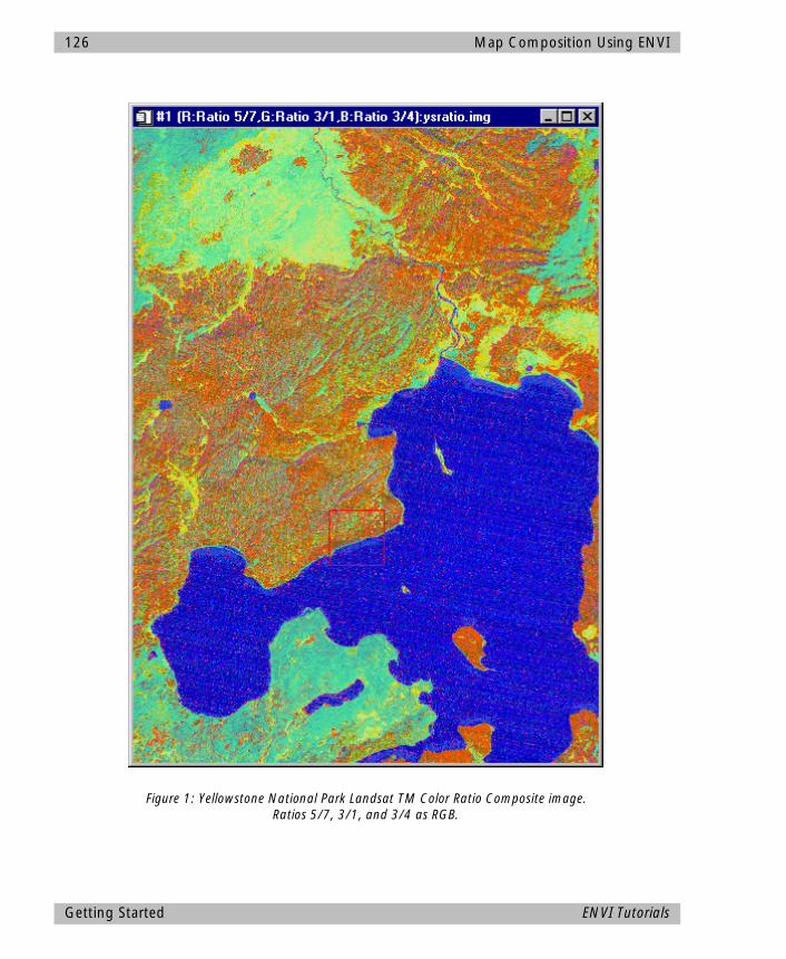
126 Map Composition Using ENVI
Figure 1: Yellowstone National Park Landsat TM Color Ratio Composite image. Ratios 5/7, 3/1, and 3/4 as RGB.
Getting Started ENVI Tutorials
Map Composition Using ENVI 127
Once the image is displayed, follow the steps below for individual components and the sequence of map composition.
Image Display and Map LayoutThe ENVI Main Display window, Scroll window, and/or Zoom window are used to perform map composition.
Virtual BordersDefault ENVI displays contain only the image, with no surrounding blank space. Map composition typically requires that some map objects reside outside the image proper. ENVI provides a “Virtual Border” capability that allows annotation in the image borders without creating a new image. Virtual borders can be added to an image in several ways.
• Automatically Added When Using Image Grids
1. Toggle on the Functions menu in the Main Display window by clicking the right mouse button in the display and select Functions->Overlays->Grid Lines.
A virtual border will be added to accommodate the grid. See the specific grid instructions below for information on setting up the grid. A 100-pixel border is automatically added on all sides of the image.
2. If you want to change from the default border, when the Grid Line Parameters dialog appears, choose Options->Set Display Borders to start the Display Borders dialog.
3. Enter the desired border characteristics and click “OK”.
The new virtual border characteristics will be applied immediately to the image. If you save the Grid Parameter File, the border information will be saved with the grid and will be restored when the grid parameters file is restored.
• Using the Available Bands List:
1. Select Options->Set Display Borders in the menu bar in the Available Bands List.
The Set Display Borders dialog will appear with the number of border pixels listed in text boxes that correspond to image geometry. This dialog is also used in Grids and Annotation to set the virtual border size.
2. Enter the desired values in the appropriate text boxes.
ENVI Tutorials Image Display and Map Layout
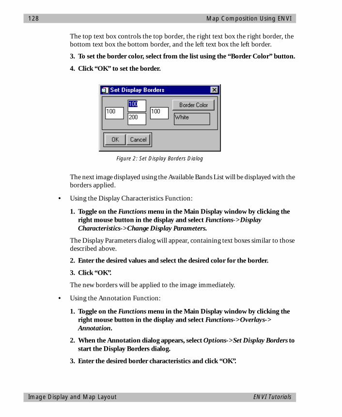
128 Map Composition Using ENVI
The top text box controls the top border, the right text box the right border, the bottom text box the bottom border, and the left text box the left border.
3. To set the border color, select from the list using the “Border Color” button.
4. Click “OK” to set the border.
The next image displayed using the Available Bands List will be displayed with the borders applied.
• Using the Display Characteristics Function:
1. Toggle on the Functions menu in the Main Display window by clicking the right mouse button in the display and select Functions->Display Characteristics->Change Display Parameters.
The Display Parameters dialog will appear, containing text boxes similar to those described above.
2. Enter the desired values and select the desired color for the border.
3. Click “OK”.
The new borders will be applied to the image immediately.
• Using the Annotation Function:
1. Toggle on the Functions menu in the Main Display window by clicking the right mouse button in the display and select Functions->Overlays-> Annotation.
2. When the Annotation dialog appears, select Options->Set Display Borders to start the Display Borders dialog.
3. Enter the desired border characteristics and click “OK”.
Figure 2: Set Display Borders Dialog
Image Display and Map Layout ENVI Tutorials
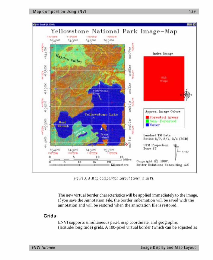
Map Composition Using ENVI 129
The new virtual border characteristics will be applied immediately to the image. If you save the Annotation File, the border information will be saved with the annotation and will be restored when the annotation file is restored.
GridsENVI supports simultaneous pixel, map coordinate, and geographic (latitude/longitude) grids. A 100-pixel virtual border (which can be adjusted as
Figure 3: A Map Composition Layout Screen in ENVI.
ENVI Tutorials Image Display and Map Layout
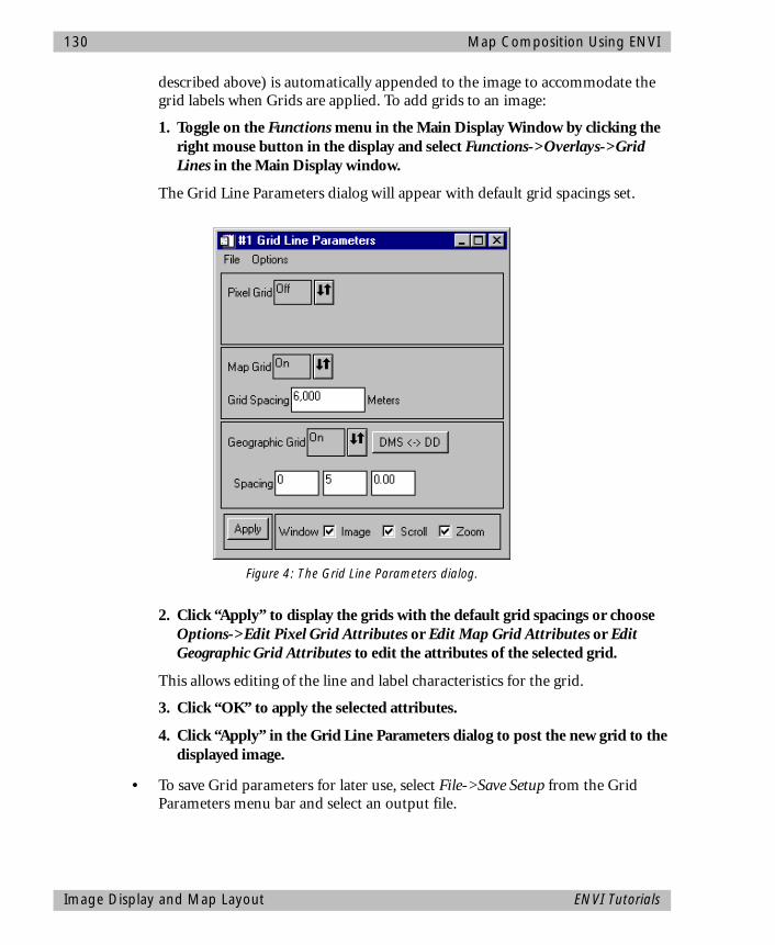
130 Map Composition Using ENVI
described above) is automatically appended to the image to accommodate the grid labels when Grids are applied. To add grids to an image:
1. Toggle on the Functions menu in the Main Display Window by clicking the right mouse button in the display and select Functions->Overlays->Grid Lines in the Main Display window.
The Grid Line Parameters dialog will appear with default grid spacings set.
2. Click “Apply” to display the grids with the default grid spacings or choose Options->Edit Pixel Grid Attributes or Edit Map Grid Attributes or Edit Geographic Grid Attributes to edit the attributes of the selected grid.
This allows editing of the line and label characteristics for the grid.
3. Click “OK” to apply the selected attributes.
4. Click “Apply” in the Grid Line Parameters dialog to post the new grid to the displayed image.
• To save Grid parameters for later use, select File->Save Setup from the Grid Parameters menu bar and select an output file.
Figure 4: The Grid Line Parameters dialog.
Image Display and Map Layout ENVI Tutorials

Map Composition Using ENVI 131
This saves a template of the grid parameters, which can be recalled for use on another map composition by choosing File ->Restore Setup from the Grid Parameters menu bar.
AnnotationAnnotation is used as a generalized means of inserting map objects into an ENVI display for map composition. Several classes of map objects are available and all are placed using ENVI’s standardized annotation procedures.
1. Toggle on the Functions menu in the Main Display window by clicking the right mouse button in the display and select Functions->Overlays-> Annotation to start the Annotation dialog.
2. Choose the desired annotation object from the Object pulldown menu in the Annotation dialog menu bar.
3. Place the object by dragging using the left mouse button and clicking the right mouse button to lock the annotation in position.
• All annotation objects can be reselected, modified, and moved by choosing Object->Selection/Edit followed by selecting the object by drawing a box around it using the left mouse button.
• Clicking the right mouse button re-locks the annotation.
The various types of annotation available in ENVI are discussed below. Please see the ENVI User’s Guide or the ENVI On-Line Help for more details.
Text and Symbols ENVI currently has 14 standard text fonts and 3 different standard symbol sets. In addition, ENVI can utilize TrueType fonts installed on your system. This provides access to a wide range of different text fonts and symbols. All of these can be interactively scaled and rotated, and different colors and thickness can be set.
1. Select Object ->Text or Object ->Symbol from the Annotation menu bar.
2. For text annotation, select the font from the pulldown font button in the left center of the dialog. Select size, color, and orientation parameters using the appropriate buttons and text entry boxes in the center of the dialog.
Figure 6: Text Annotation.
ENVI Tutorials Image Display and Map Layout
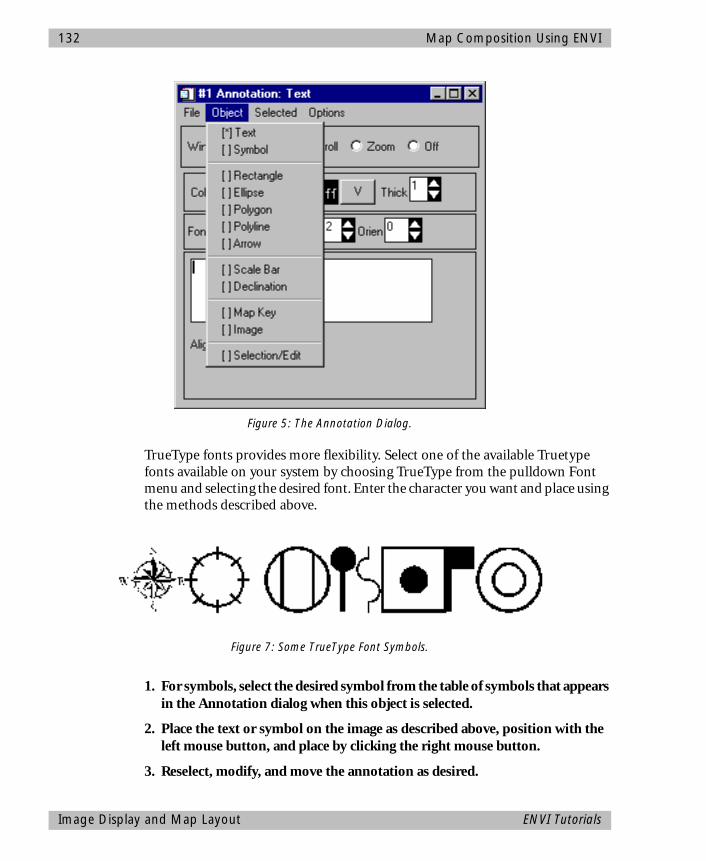
132 Map Composition Using ENVI
TrueType fonts provides more flexibility. Select one of the available Truetype fonts available on your system by choosing TrueType from the pulldown Font menu and selecting the desired font. Enter the character you want and place using the methods described above.
1. For symbols, select the desired symbol from the table of symbols that appears in the Annotation dialog when this object is selected.
2. Place the text or symbol on the image as described above, position with the left mouse button, and place by clicking the right mouse button.
3. Reselect, modify, and move the annotation as desired.
Figure 5: The Annotation Dialog.
Figure 7: Some TrueType Font Symbols.
Image Display and Map Layout ENVI Tutorials
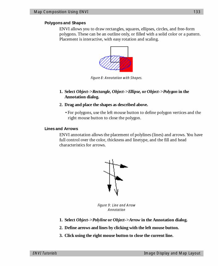
Map Composition Using ENVI 133
Polygons and Shapes ENVI allows you to draw rectangles, squares, ellipses, circles, and free-form polygons. These can be an outline only, or filled with a solid color or a pattern. Placement is interactive, with easy rotation and scaling.
1. Select Object->Rectangle, Object->Ellipse, or Object->Polygon in the Annotation dialog.
2. Drag and place the shapes as described above.
• For polygons, use the left mouse button to define polygon vertices and the right mouse button to close the polygon.
Lines and Arrows ENVI annotation allows the placement of polylines (lines) and arrows. You have full control over the color, thickness and linetype, and the fill and head characteristics for arrows.
1. Select Object->Polyline or Object->Arrow in the Annotation dialog.
2. Define arrows and lines by clicking with the left mouse button.
3. Click using the right mouse button to close the current line.
Figure 8: Annotation with Shapes.
Figure 9: Line and Arrow Annotation
ENVI Tutorials Image Display and Map Layout

134 Map Composition Using ENVI
Map Scales Map Scales are automatically generated by ENVI based on the pixel size of the image being used in the map composition. Options include feet, miles, meters, and kilometers. Scales can be placed individually, or in groups. The number of divisions and minor divisions is completely configurable, as is the font and the character size.
1. Select Object->Scale Bar in the Annotation dialog.
2. Enter the desired parameters, then place the scale bar using the left mouse button.
3. Lock in the annotation using the right mouse button.
Declination ENVI automatically generates declination diagrams based on user-provided characteristics. The size of the diagram and the azimuths for True North, Grid North, and Magnetic North are entered in decimal degrees and the diagram is placed using standard ENVI annotation procedure.
1. Select Object->Declination in the Annotation dialog.
2. Place the annotation using the left mouse button.
3. Lock in the annotation using the right mouse button.
Map Keys Shown below is an example of a map key build using ENVI’s map key editing facility. The box around the key is a rectangle placed as a separate annotation object as is the key description at the top of the box.
1. Select Object ->Map Key in the Annotation dialog.
2. Choose Edit Map Key Items to add, delete, or modify individual map key items.
3. Place the map key using the left mouse button and lock in using the right mouse button.
Figure 10: Scale Bar Annotation.
Image Display and Map Layout ENVI Tutorials
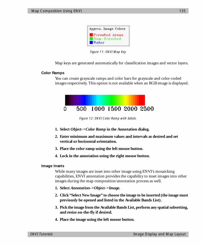
Map Composition Using ENVI 135
Map keys are generated automatically for classification images and vector layers.
Color Ramps You can create grayscale ramps and color bars for grayscale and color-coded images respectively. This option is not available when an RGB image is displayed.
1. Select Object->Color Ramp in the Annotation dialog.
2. Enter minimum and maximum values and intervals as desired and set vertical or horizontal orientation.
3. Place the color ramp using the left mouse button.
4. Lock in the annotation using the right mouse button.
Image Insets While many images are inset into other image using ENVI’s mosaicking capabilities, ENVI annotation provides the capability to inset images into other images during the map composition/annotation process as well.
1. Select Annotation->Object->Image.
2. Click “Select New Image” to choose the image to be inserted (the image must previously be opened and listed in the Available Bands List).
3. Pick the image from the Available Bands List, perform any spatial subsetting, and resize on-the-fly if desired.
4. Place the image using the left mouse button.
Figure 11: ENVI Map Key
Figure 12: ENVI Color Ramp with labels.
ENVI Tutorials Image Display and Map Layout

136 Map Composition Using ENVI
5. Lock the image in using the right mouse button.
Because 8-bit displays can not easily assign a new color table to the inset image, ENVI only shows a representation of the image in the display window. The actual image is placed when the image is output to a file and the annotation is burnt in.
Vector LayersENVI can import ArcShape, Arc/Info Interchange, DXF, and DLG vector formats. Vectors from these files and internal ENVI Vector Files (.evf) can be used in an ENVI map composition.
1. Open the files by selecting File->Open Vector File->the appropriate file type.
2. Load the vectors into the map composition display, by clicking on Apply and adjust the attributes to obtain the desired colors, thickness, and linetypes. See the Vector Overlay and GIS Analysis Tutorial in this volume or see the ENVI User’s Guide or on-line help for additional information.
OutputThe image-map composition can be output from the Main Display window.
1. Set the annotation to “Off” in the Annotation dialog.
2. Click the right mouse button in the Main Display window and select Functions->Output Display->the desired output type.
Options include Postscript, ENVI (binary) image, BMP, GIF, HDF, JPEG, PICT, SRF, TIFF, and XWD, as well as common image processing system formats such as PCI, ERDAS, ERMAPPER, and ArcView Raster.
You can also select direct printing, in which case, the map composition will be printed directly to your hardware using system software drivers.
In all of the above cases, graphics and map composition objects will be burned into the image on output.
The figure on the following page shows an example of a finsl map composition produced in ENVI.
Image Display and Map Layout ENVI Tutorials
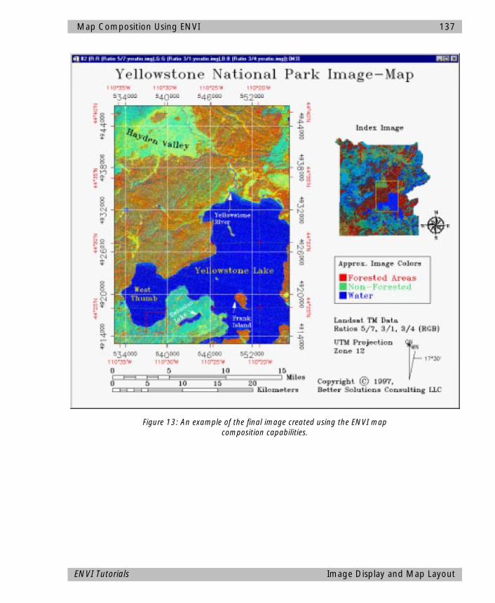
Map Composition Using ENVI 137
Figure 13: An example of the final image created using the ENVI map composition capabilities.
ENVI Tutorials Image Display and Map Layout

138 Map Composition Using ENVI
Image Display and Map Layout ENVI Tutorials

ENVI Tutorial #7
Introduction to Hyperspectral Data and Analysis
The following topics are covered in this tutorial:
IOverview of This Tutorial......................................................................................140Background: Imaging Spectrometry......................................................................141Introduction to Basic ENVI Functionality ...............................................................141Working With Cuprite Radiance Data ....................................................................148Comparison of Radiance and ATREM Reflectance ..................................................152Compare Different Calibrations.............................................................................155
139
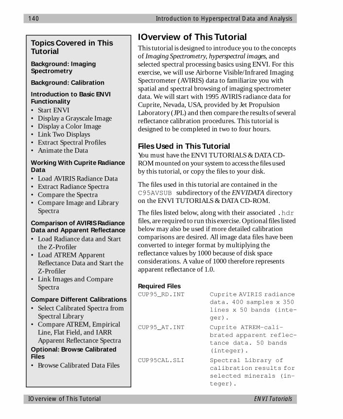
140 Introduction to Hyperspectral Data and Analysis
IOverview of This TutorialThis tutorial is designed to introduce you to the concepts of Imaging Spectrometry, hyperspectral images, and selected spectral processing basics using ENVI. For this exercise, we will use Airborne Visible/Infrared Imaging Spectrometer (AVIRIS) data to familiarize you with spatial and spectral browsing of imaging spectrometer data. We will start with 1995 AVIRIS radiance data for Cuprite, Nevada, USA, provided by Jet Propulsion Laboratory (JPL) and then compare the results of several reflectance calibration procedures. This tutorial is designed to be completed in two to four hours.
Files Used in This TutorialYou must have the ENVI TUTORIALS & DATA CD-ROM mounted on your system to access the files usedby this tutorial, or copy the files to your disk.
The files used in this tutorial are contained in the C95AVSUB subdirectory of the ENVIDATA directory on the ENVI TUTORIALS & DATA CD-ROM.
The files listed below, along with their associated .hdr files, are required to run this exercise. Optional files listed below may also be used if more detailed calibration comparisons are desired. All image data files have been converted to integer format by multiplying the reflectance values by 1000 because of disk space considerations. A value of 1000 therefore represents apparent reflectance of 1.0.
Required FilesCUP95_RD.INT Cuprite AVIRIS radiance
data. 400 samples x 350 lines x 50 bands (inte-ger).
CUP95_AT.INT Cuprite ATREM-cali-brated apparent reflec-tance data. 50 bands (integer).
CUP95CAL.SLI Spectral Library of calibration results for selected minerals (in-teger).
Topics Covered in This Tutorial
Background: Imaging Spectrometry
Background: Calibration
Introduction to Basic ENVI Functionality• Start ENVI• Display a Grayscale Image• Display a Color Image• Link Two Displays• Extract Spectral Profiles• Animate the Data
Working With Cuprite Radiance Data• Load AVIRIS Radiance Data• Extract Radiance Spectra• Compare the Spectra• Compare Image and Library
Spectra
Comparison of AVIRIS Radiance Data and Apparent Reflectance• Load Radiance data and Start
the Z-Profiler• Load ATREM Apparent
Reflectance Data and Start the Z-Profiler
• Link Images and Compare Spectra
Compare Different Calibrations• Select Calibrated Spectra from
Spectral Library• Compare ATREM, Empirical
Line, Flat Field, and IARR Apparent Reflectance Spectra
Optional: Browse Calibrated Files• Browse Calibrated Data Files
IOverview of This Tutorial ENVI Tutorials
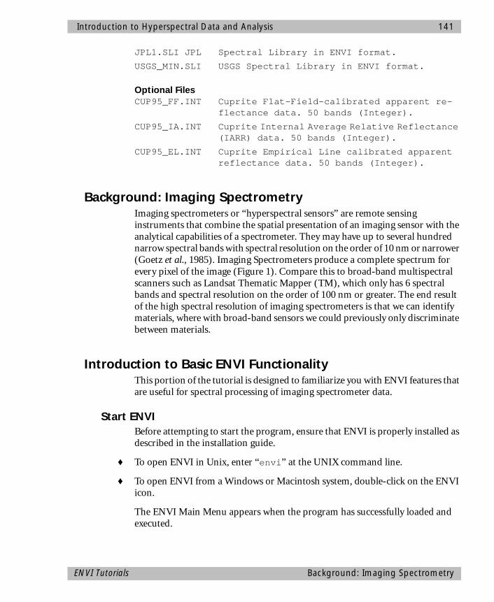
Introduction to Hyperspectral Data and Analysis 141
JPL1.SLI JPL Spectral Library in ENVI format.
USGS_MIN.SLI USGS Spectral Library in ENVI format.
Optional FilesCUP95_FF.INT Cuprite Flat-Field-calibrated apparent re-
flectance data. 50 bands (Integer).
CUP95_IA.INT Cuprite Internal Average Relative Reflectance (IARR) data. 50 bands (Integer).
CUP95_EL.INT Cuprite Empirical Line calibrated apparent reflectance data. 50 bands (Integer).
Background: Imaging SpectrometryImaging spectrometers or “hyperspectral sensors” are remote sensing instruments that combine the spatial presentation of an imaging sensor with the analytical capabilities of a spectrometer. They may have up to several hundred narrow spectral bands with spectral resolution on the order of 10 nm or narrower (Goetz et al., 1985). Imaging Spectrometers produce a complete spectrum for every pixel of the image (Figure 1). Compare this to broad-band multispectral scanners such as Landsat Thematic Mapper (TM), which only has 6 spectral bands and spectral resolution on the order of 100 nm or greater. The end result of the high spectral resolution of imaging spectrometers is that we can identify materials, where with broad-band sensors we could previously only discriminate between materials.
Introduction to Basic ENVI FunctionalityThis portion of the tutorial is designed to familiarize you with ENVI features that are useful for spectral processing of imaging spectrometer data.
Start ENVIBefore attempting to start the program, ensure that ENVI is properly installed as described in the installation guide.
♦ To open ENVI in Unix, enter “envi” at the UNIX command line.
♦ To open ENVI from a Windows or Macintosh system, double-click on the ENVI icon.
The ENVI Main Menu appears when the program has successfully loaded and executed.
ENVI Tutorials Background: Imaging Spectrometry
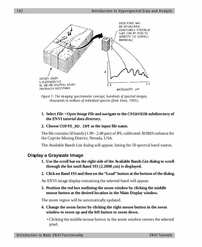
142 Introduction to Hyperspectral Data and Analysis
1. Select File->Open Image File and navigate to the C95AVSUB subdirectory of the ENVI tutorial data directory.
2. Choose CUP95_RD.INT as the input file name.
The file contains 50 bands (1.99 - 2.48 µm) of JPL-calibrated AVIRIS radiance for the Cuprite Mining District, Nevada, USA.
The Available Bands List dialog will appear, listing the 50 spectral band names.
Display a Grayscale Image1. Use the scroll bar on the right side of the Available Bands List dialog to scroll
through the list until Band 193 (2.2008 µm) is displayed.
2. Click on Band 193 and then on the “Load” button at the bottom of the dialog.
An ENVI image display containing the selected band will appear.
3. Position the red box outlining the zoom window by clicking the middle mouse button at the desired location in the Main Display window.
The zoom region will be automatically updated.
4. Change the zoom factor by clicking the right mouse button in the zoom window to zoom up and the left button to zoom down.
• Clicking the middle mouse button in the zoom window centers the selected pixel.
Figure 1: The imaging spectrometer concept; hundreds of spectral images, thousands to millions of individual spectra (from Vane, 1985).
Introduction to Basic ENVI Functionality ENVI Tutorials
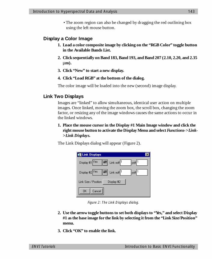
Introduction to Hyperspectral Data and Analysis 143
• The zoom region can also be changed by dragging the red outlining box using the left mouse button.
Display a Color Image1. Load a color composite image by clicking on the “RGB Color” toggle button
in the Available Bands List.
2. Click sequentially on Band 183, Band 193, and Band 207 (2.10, 2.20, and 2.35 µm).
3. Click “New” to start a new display.
4. Click “Load RGB” at the bottom of the dialog.
The color image will be loaded into the new (second) image display.
Link Two DisplaysImages are “linked” to allow simultaneous, identical user action on multiple images. Once linked, moving the zoom box, the scroll box, changing the zoom factor, or resizing any of the image windows causes the same actions to occur in the linked windows.
1. Place the mouse cursor in the Display #1 Main Image window and click the right mouse button to activate the Display Menu and select Functions->Link->Link Displays.
The Link Displays dialog will appear (Figure 2).
2. Use the arrow toggle buttons to set both displays to “Yes,” and select Display #1 as the base image for the link by selecting it from the “Link Size/Position” menu.
3. Click “OK” to enable the link.
Figure 2: The Link Displays dialog.
ENVI Tutorials Introduction to Basic ENVI Functionality

144 Introduction to Hyperspectral Data and Analysis
4. Position the Zoom window for Display #1 by clicking the left mouse button in the red Zoom Window outlining box in the #1 Main Image Display and dragging it to a new location.
Note how the Display #2 Zoom window updates to correspond with the first display.
“Multiple Dynamic Overlays” are available when two or more images are linked, allowing real-time overlay and toggling (flicker) of multiple grayscale or color images. Dynamic overlays are activated automatically when two or more windows are first linked.
5. After linking, click the left mouse button in either of the linked images to cause a small portion of the second linked image (the overlay) to appear in the first image (the base).
6. You can make a quick visual comparison of the images by repeatedly clicking and releasing the left mouse button, which causes the overlay area to “flicker.”
7. Change the size of the overlay by pressing the middle mouse button and dragging the corner of the overlay to the desired location.
8. After trying the different possibilities, turn off dynamic linking in Display 1 by selecting Functions->Link->Dynamic Overlay Off.
Extract Spectral ProfilesENVI’s “Z” profile capabilities provide integrated spectral analysis. You can extract spectra from any multispectral data set including MSS, TM, and higher spectral dimension data such as GEOSCAN (24 bands), GERIS (63 bands), and AVIRIS (224 bands).
1. Select Functions->Profiles->Z Profile in the Display 1 Main window.
Current SpectrumThe spectrum for the current cursor location will be plotted in a plot window. A vertical line on the plot is used to mark the wavelength position of the currently displayed band. If a color composite image is displayed, three colored lines will appear, one for each displayed band in the band’s respective color (red, green, or blue).
2. Move the cursor position in the Main or Zoom window.
The spectrum will be extracted and plotted for the new location.
Introduction to Basic ENVI Functionality ENVI Tutorials
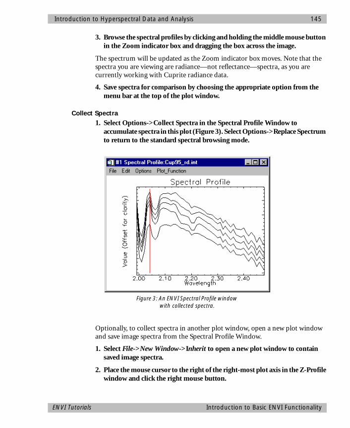
Introduction to Hyperspectral Data and Analysis 145
3. Browse the spectral profiles by clicking and holding the middle mouse button in the Zoom indicator box and dragging the box across the image.
The spectrum will be updated as the Zoom indicator box moves. Note that the spectra you are viewing are radiance—not reflectance—spectra, as you are currently working with Cuprite radiance data.
4. Save spectra for comparison by choosing the appropriate option from the menu bar at the top of the plot window.
Collect Spectra1. Select Options->Collect Spectra in the Spectral Profile Window to
accumulate spectra in this plot (Figure 3). Select Options->Replace Spectrum to return to the standard spectral browsing mode.
Optionally, to collect spectra in another plot window, open a new plot window and save image spectra from the Spectral Profile Window.
1. Select File->New Window->Inherit to open a new plot window to contain saved image spectra.
2. Place the mouse cursor to the right of the right-most plot axis in the Z-Profile window and click the right mouse button.
Figure 3: An ENVI Spectral Profile window with collected spectra.
ENVI Tutorials Introduction to Basic ENVI Functionality

146 Introduction to Hyperspectral Data and Analysis
The spectrum name will be displayed to the right of the plot.
3. Click and hold the left mouse button on the first character of the spectrum name, drag the name to the new plot window, and release the mouse button.
4. Select a new spectrum from the image by moving the current pixel location in either the Main Display or Zoom window and repeat the drag-and-drop process to build a collection of spectra in the new plot window.
5. Once you have several plots in the plot window, select Options->Stack Data in the plot window.
The spectra will be offset vertically to allow interpretation.
6. To change the color and line style of the different spectra, select Edit->Data Parameters in the new plot window.
Each spectrum is listed by name/location in the Data Parameters dialog.
7. Select a line and change its properties as desired.
8. When completed, click “Cancel” to close the dialog.
9. Select File->Cancel to close the plots after completing this section.
Animate the DataYou can “animate” grayscale images to make the spatial occurrence of spectral differences more obvious.
1. In the Main window of the grayscale image (Display #1), select Functions-> Interactive Analysis->Animation to create a “movie” using the Cuprite AVIRIS data.
The Animation Input Parameters dialog will appear, listing the bands (Figure 4).
2. Choose a subset of the full set of bands for animation.
3. Click “Clear” in the Animation Input Parameters dialog.
4. Click either on the check boxes to the left of bands 12 - 31 (20 bands), or enter 12 and 31 in the text boxes next to the “Add Range” button and click on the button to select the spectral bands.
5. Change the “Window Size” to 200 x 175 to reduce the size of the image to be animated (and thus increase the speed of the animation).
6. Click “OK” to return to the Animation Input Parameters dialog.
7. Click “OK” again to start the animation loading process.
Introduction to Basic ENVI Functionality ENVI Tutorials
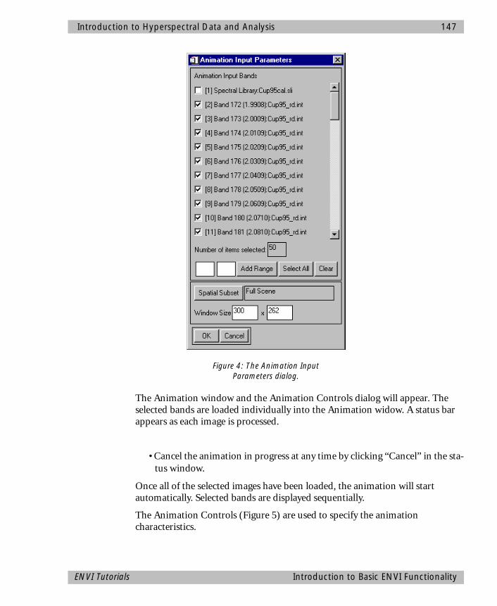
Introduction to Hyperspectral Data and Analysis 147
The Animation window and the Animation Controls dialog will appear. The selected bands are loaded individually into the Animation widow. A status bar appears as each image is processed.
• Cancel the animation in progress at any time by clicking “Cancel” in the sta-tus window.
Once all of the selected images have been loaded, the animation will start automatically. Selected bands are displayed sequentially.
The Animation Controls (Figure 5) are used to specify the animation characteristics.
Figure 4: The Animation Input Parameters dialog.
ENVI Tutorials Introduction to Basic ENVI Functionality
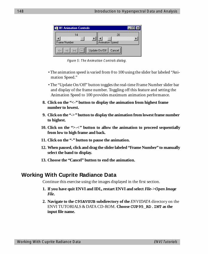
148 Introduction to Hyperspectral Data and Analysis
• The animation speed is varied from 0 to 100 using the slider bar labeled “Ani-mation Speed.”
• The “Update On/Off” button toggles the real-time Frame Number slider bar and display of the frame number. Toggling off this feature and setting the Animation Speed to 100 provides maximum animation performance.
8. Click on the “<-” button to display the animation from highest frame number to lowest.
9. Click on the “->” button to display the animation from lowest frame number to highest.
10. Click on the “>-<” button to allow the animation to proceed sequentiallyfrom low to high frame and back.
11. Click on the “-” button to pause the animation.
12. When paused, click and drag the slider labeled “Frame Number” to manuallyselect the band to display.
13. Choose the “Cancel” button to end the animation.
Working With Cuprite Radiance DataContinue this exercise using the images displayed in the first section.
1. If you have quit ENVI and IDL, restart ENVI and select File->Open Image File.
2. Navigate to the C95AVSUB subdirectory of the ENVIDATA directory on the ENVI TUTORIALS & DATA CD-ROM. Choose CUP95_RD.INT as the input file name.
Figure 5: The Animation Controls dialog.
Working With Cuprite Radiance Data ENVI Tutorials

Introduction to Hyperspectral Data and Analysis 149
Load AVIRIS Radiance Data1. If you don’t already have this image displayed, load a color composite image
by clicking on the “RGB Color” toggle button in the Available Bands List.
2. Click sequentially on Band 183, Band 193, and Band 207 and then “Load RGB” at the bottom of the dialog.
The color image will be loaded into the current image display.
Extract Radiance SpectraTo extract selected image radiance spectra for specific targets in the AVIRIS radiance data.
1. In the Main Display window, select Functions->Interactive Analysis->Pixel Locator.
2. Position the zoom window over Stonewall Playa, centered around the pixel at sample 590, line 570 by entering these pixel coordinates in the Pixel Locator and clicking “Apply”.
3. Extract the radiance spectrum for this location using the Z-Profile function and save in a new plot window.
4. Extract radiance spectra for the following locations and load into the same plot window for comparison (Figure 6).
• Change the colors of the individual plots if necessary by selecting Edit-> Data Parameters and making the appropriate changes in the subsequent dia-log.
Location NameSample(with offset)
Line(with offset)
Stonewall Playa 590 570
Varnished Tuff 435 555
Silica Cap 494 514
Opalite Zone with Alunite 531 541
Strongly Argillized Zone with Kaolinite
502 589
Buddingtonite Zone 448 505
Calcite 260 613
ENVI Tutorials Working With Cuprite Radiance Data
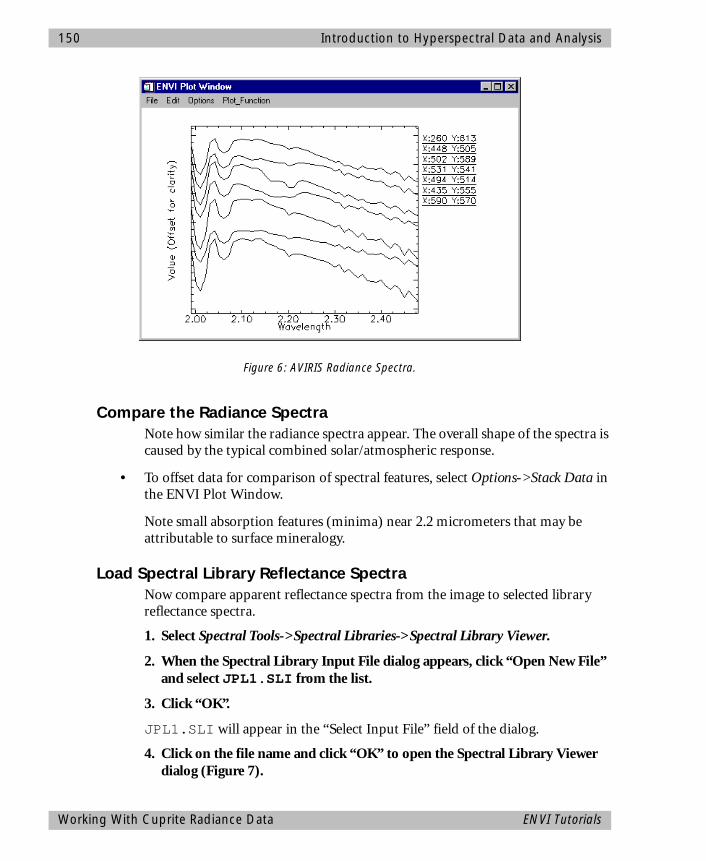
150 Introduction to Hyperspectral Data and Analysis
Compare the Radiance SpectraNote how similar the radiance spectra appear. The overall shape of the spectra is caused by the typical combined solar/atmospheric response.
• To offset data for comparison of spectral features, select Options->Stack Data in the ENVI Plot Window.
Note small absorption features (minima) near 2.2 micrometers that may be attributable to surface mineralogy.
Load Spectral Library Reflectance SpectraNow compare apparent reflectance spectra from the image to selected library reflectance spectra.
1. Select Spectral Tools->Spectral Libraries->Spectral Library Viewer.
2. When the Spectral Library Input File dialog appears, click “Open New File” and select JPL1.SLI from the list.
3. Click “OK”.
JPL1.SLI will appear in the “Select Input File” field of the dialog.
4. Click on the file name and click “OK” to open the Spectral Library Viewer dialog (Figure 7).
Figure 6: AVIRIS Radiance Spectra.
Working With Cuprite Radiance Data ENVI Tutorials
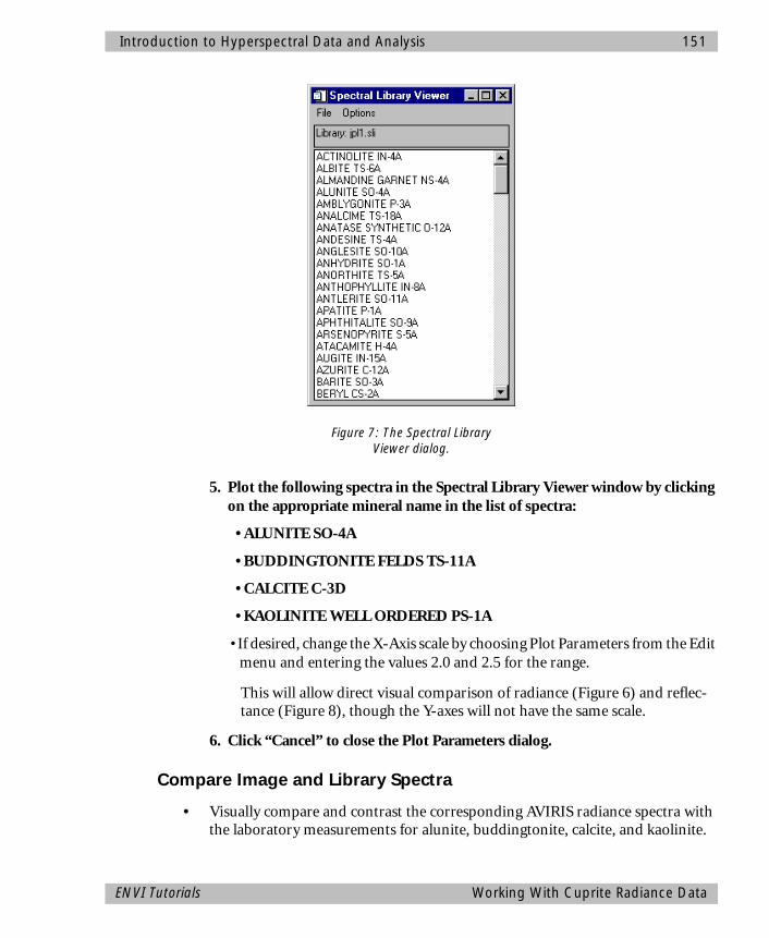
Introduction to Hyperspectral Data and Analysis 151
5. Plot the following spectra in the Spectral Library Viewer window by clicking on the appropriate mineral name in the list of spectra:
• ALUNITE SO-4A
• BUDDINGTONITE FELDS TS-11A
• CALCITE C-3D
• KAOLINITE WELL ORDERED PS-1A
• If desired, change the X-Axis scale by choosing Plot Parameters from the Edit menu and entering the values 2.0 and 2.5 for the range.
This will allow direct visual comparison of radiance (Figure 6) and reflec-tance (Figure 8), though the Y-axes will not have the same scale.
6. Click “Cancel” to close the Plot Parameters dialog.
Compare Image and Library Spectra
• Visually compare and contrast the corresponding AVIRIS radiance spectra with the laboratory measurements for alunite, buddingtonite, calcite, and kaolinite.
Figure 7: The Spectral Library Viewer dialog.
ENVI Tutorials Working With Cuprite Radiance Data
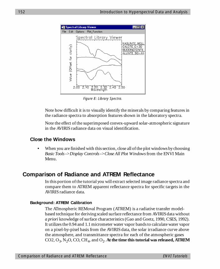
152 Introduction to Hyperspectral Data and Analysis
Note how difficult it is to visually identify the minerals by comparing features in the radiance spectra to absorption features shown in the laboratory spectra.
Note the effect of the superimposed convex-upward solar-atmospheric signature in the AVIRIS radiance data on visual identification.
Close the Windows
• When you are finished with this section, close all of the plot windows by choosing Basic Tools ->Display Controls ->Close All Plot Windows from the ENVI Main Menu.
Comparison of Radiance and ATREM ReflectanceIn this portion of the tutorial you will extract selected image radiance spectra and compare them to ATREM apparent reflectance spectra for specific targets in the AVIRIS radiance data.
Background: ATREM CalibrationThe ATmospheric REMoval Program (ATREM) is a radiative transfer model-based technique for deriving scaled surface reflectance from AVIRIS data without a priori knowledge of surface characteristics (Gao and Goetz, 1990, CSES, 1992). It utilizes the 0.94 and 1.1 micrometer water vapor bands to calculate water vapor on a pixel-by-pixel basis from the AVIRIS data, the solar irradiance curve above the atmosphere, and transmittance spectra for each of the atmospheric gases CO2, O3, N2O, CO, CH4, and O2. At the time this tutorial was released, ATREM
Figure 8: Library Spectra.
Comparison of Radiance and ATREM Reflectance ENVI Tutorials
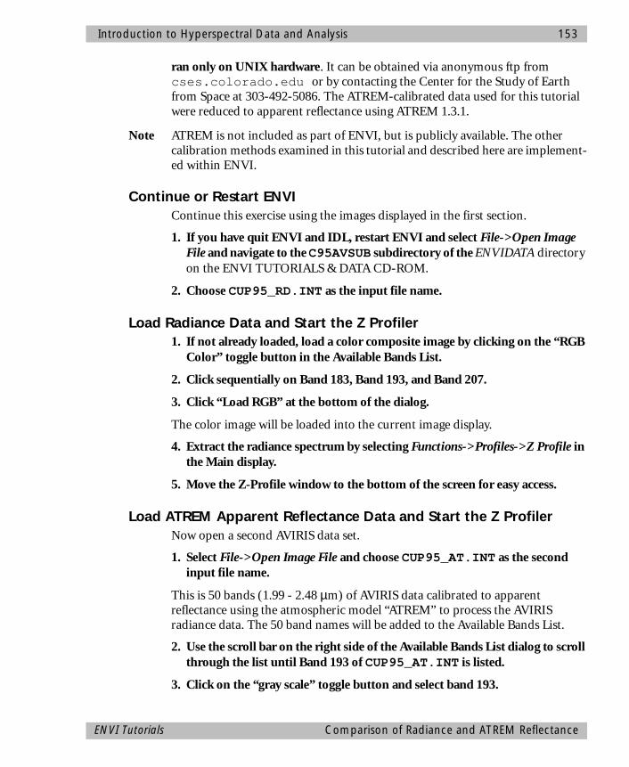
Introduction to Hyperspectral Data and Analysis 153
ran only on UNIX hardware. It can be obtained via anonymous ftp from cses.colorado.edu or by contacting the Center for the Study of Earth from Space at 303-492-5086. The ATREM-calibrated data used for this tutorial were reduced to apparent reflectance using ATREM 1.3.1.
Note ATREM is not included as part of ENVI, but is publicly available. The other calibration methods examined in this tutorial and described here are implement-ed within ENVI.
Continue or Restart ENVIContinue this exercise using the images displayed in the first section.
1. If you have quit ENVI and IDL, restart ENVI and select File->Open Image File and navigate to the C95AVSUB subdirectory of the ENVIDATA directory on the ENVI TUTORIALS & DATA CD-ROM.
2. Choose CUP95_RD.INT as the input file name.
Load Radiance Data and Start the Z Profiler1. If not already loaded, load a color composite image by clicking on the “RGB
Color” toggle button in the Available Bands List.
2. Click sequentially on Band 183, Band 193, and Band 207.
3. Click “Load RGB” at the bottom of the dialog.
The color image will be loaded into the current image display.
4. Extract the radiance spectrum by selecting Functions->Profiles->Z Profile in the Main display.
5. Move the Z-Profile window to the bottom of the screen for easy access.
Load ATREM Apparent Reflectance Data and Start the Z ProfilerNow open a second AVIRIS data set.
1. Select File->Open Image File and choose CUP95_AT.INT as the second input file name.
This is 50 bands (1.99 - 2.48 µm) of AVIRIS data calibrated to apparent reflectance using the atmospheric model “ATREM” to process the AVIRIS radiance data. The 50 band names will be added to the Available Bands List.
2. Use the scroll bar on the right side of the Available Bands List dialog to scroll through the list until Band 193 of CUP95_AT.INT is listed.
3. Click on the “gray scale” toggle button and select band 193.
ENVI Tutorials Comparison of Radiance and ATREM Reflectance

154 Introduction to Hyperspectral Data and Analysis
4. Click “New” and then “Load” to start a second ENVI image display and load the selected band.
5. Extract the radiance spectrum by selecting Functions->Profiles->Z Profile in the Main window.
6. Move the Z-Profile window to the bottom of the screen next to the Z-Profile from the radiance data for easy comparison.
Link Images and Compare Spectra1. Link the two AVIRIS images together by selecting Functions->Link from the
#1 Display Main window and clicking “OK” in the subsequent Link Displays dialog.
2. Now turn the dynamic overlay off in Display #1 by selecting Functions->Link->Dynamic Overlay Off.
3. Once the images are linked and the overlay is turned off, positioning the current pixel in one image (either by clicking the center mouse button in the image, dragging the zoom indicator box using the left mouse button, or by using the Pixel Locator) will also position the cursor in the second image.
The Z profiles for both images will change to show the radiance and apparent reflectance spectra at the current location.
4. Position the zoom window over Stonewall Playa, centered around the pixel at sample 590, line 570 (use the Pixel Locator dialog found in the Interactive Analysis cascading menu under the Functions menu).
Visually compare both radiance and apparent reflectance spectrum for this location using the two Z-Profiles.
• If you wish, save the radiance spectrum in one new plot window and the reflectance spectrum in a second new plot window.
• Use the middle mouse button to the left of the Y-axis to scale spectra to fit in the window.
5. Now extract radiance and apparent reflectance spectra for the following locations and visually compare.
Comparison of Radiance and ATREM Reflectance ENVI Tutorials
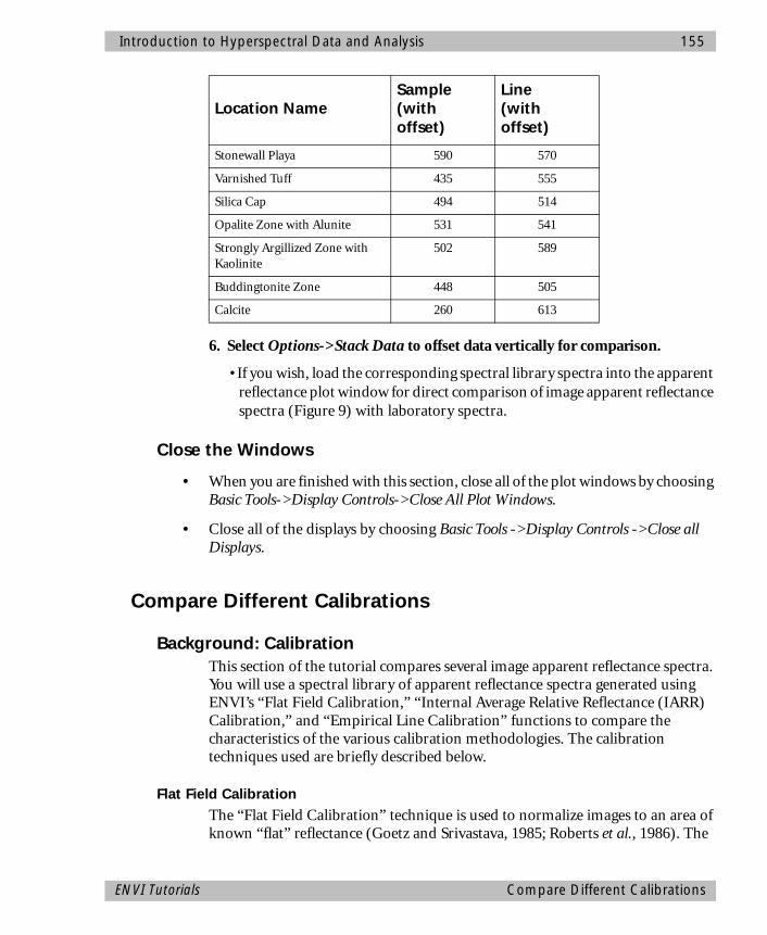
Introduction to Hyperspectral Data and Analysis 155
6. Select Options->Stack Data to offset data vertically for comparison.
• If you wish, load the corresponding spectral library spectra into the apparent reflectance plot window for direct comparison of image apparent reflectance spectra (Figure 9) with laboratory spectra.
Close the Windows
• When you are finished with this section, close all of the plot windows by choosing Basic Tools->Display Controls->Close All Plot Windows.
• Close all of the displays by choosing Basic Tools ->Display Controls ->Close all Displays.
Compare Different Calibrations
Background: CalibrationThis section of the tutorial compares several image apparent reflectance spectra. You will use a spectral library of apparent reflectance spectra generated using ENVI’s “Flat Field Calibration,” “Internal Average Relative Reflectance (IARR) Calibration,” and “Empirical Line Calibration” functions to compare the characteristics of the various calibration methodologies. The calibration techniques used are briefly described below.
Flat Field CalibrationThe “Flat Field Calibration” technique is used to normalize images to an area of known “flat” reflectance (Goetz and Srivastava, 1985; Roberts et al., 1986). The
Location NameSample(with offset)
Line(with offset)
Stonewall Playa 590 570
Varnished Tuff 435 555
Silica Cap 494 514
Opalite Zone with Alunite 531 541
Strongly Argillized Zone with Kaolinite
502 589
Buddingtonite Zone 448 505
Calcite 260 613
ENVI Tutorials Compare Different Calibrations
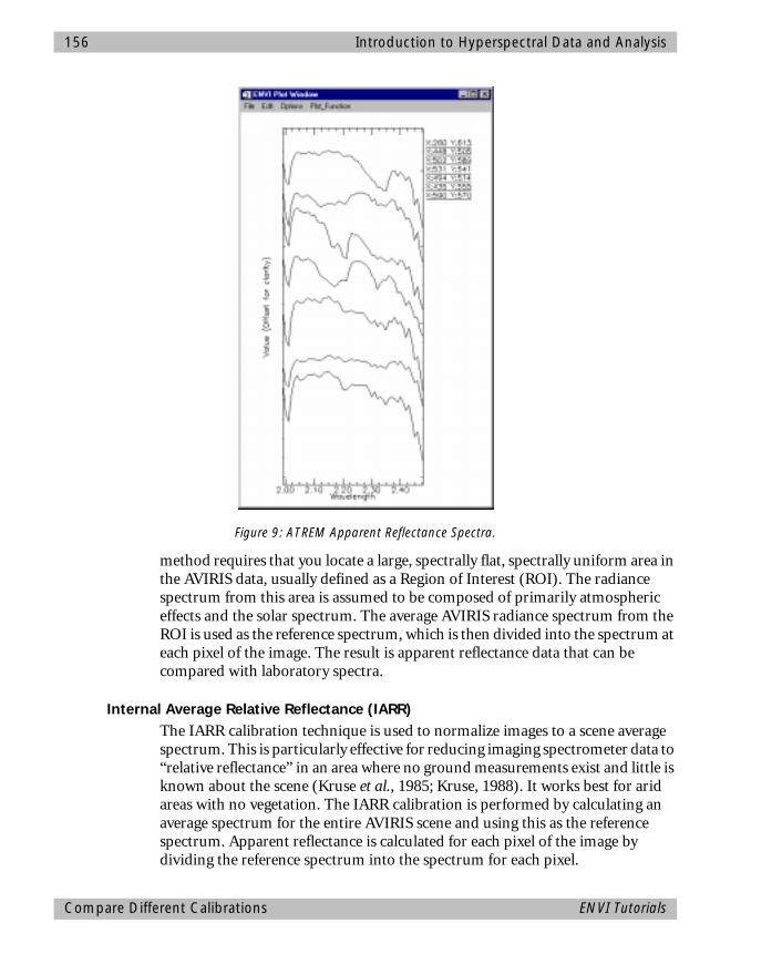
156 Introduction to Hyperspectral Data and Analysis
method requires that you locate a large, spectrally flat, spectrally uniform area in the AVIRIS data, usually defined as a Region of Interest (ROI). The radiance spectrum from this area is assumed to be composed of primarily atmospheric effects and the solar spectrum. The average AVIRIS radiance spectrum from the ROI is used as the reference spectrum, which is then divided into the spectrum at each pixel of the image. The result is apparent reflectance data that can be compared with laboratory spectra.
Internal Average Relative Reflectance (IARR)The IARR calibration technique is used to normalize images to a scene average spectrum. This is particularly effective for reducing imaging spectrometer data to “relative reflectance” in an area where no ground measurements exist and little is known about the scene (Kruse et al., 1985; Kruse, 1988). It works best for arid areas with no vegetation. The IARR calibration is performed by calculating an average spectrum for the entire AVIRIS scene and using this as the reference spectrum. Apparent reflectance is calculated for each pixel of the image by dividing the reference spectrum into the spectrum for each pixel.
Figure 9: ATREM Apparent Reflectance Spectra.
Compare Different Calibrations ENVI Tutorials

Introduction to Hyperspectral Data and Analysis 157
Empirical Line CalibrationThe Empirical Line calibration technique is used to force image data to match selected field reflectance spectra (Roberts et al., 1985; Conel et al., 1987; Kruse et al., 1990). This method requires ground measurements and/or knowledge. Two or more ground targets are identified and reflectance is measured in the field. Usually the targets consist of at least one light and one dark area. The same two targets are identified in the AVIRIS images and average spectra are extracted for Regions of Interest. A linear regression is calculated between the field reflectance spectra and the image radiance spectra to determine a linear transform from radiance to reflectance for each band of the AVIRIS data set. Gains and offsets calculated in the regression are applied to the radiance spectra for each pixel to produce apparent reflectance on a pixel-by-pixel basis.
Continue or Restart ENVI and Select Spectral Library of Calibration Results Spectra1. If you have quit ENVI and IDL, restart ENVI and select Spectral Tools-
>Spectral Libraries->Spectral Library Viewer.
The Spectral Library Input File dialog will appear to allow selection of a spectral library.
2. Click “Open New File” at the bottom center of the dialog to start a standard file selection dialog.
3. Navigate to the C95AVSUB subdirectory of the ENVIDATA directory on the ENVI TUTORIALS & DATA CD-ROM, and select the file CUP95CAL.SLI.
This is the spectral library containing the results from the various calibration methods.
4. In the Spectral Library Input File dialog, select the open library file name and click “OK”.
The Spectral Library Viewer will appear with a list of the calibrated spectra (Figure 10).
Select Calibrated Spectra from Spectral Library1. Select the ATREM, Flat Field, IARR, and Empirical Line calibrated spectra for
the mineral Alunite by clicking on the appropriate check boxes next to the names in the list.
The spectra will be plotted in a Spectral Library Viewer plot (Figure 11). Visually compare the various calibrations and note and compare their characteristics.
2. Attempt to explain some of the differences in terms of the calibration methodology used (see the brief descriptions above of the various methods).
ENVI Tutorials Compare Different Calibrations
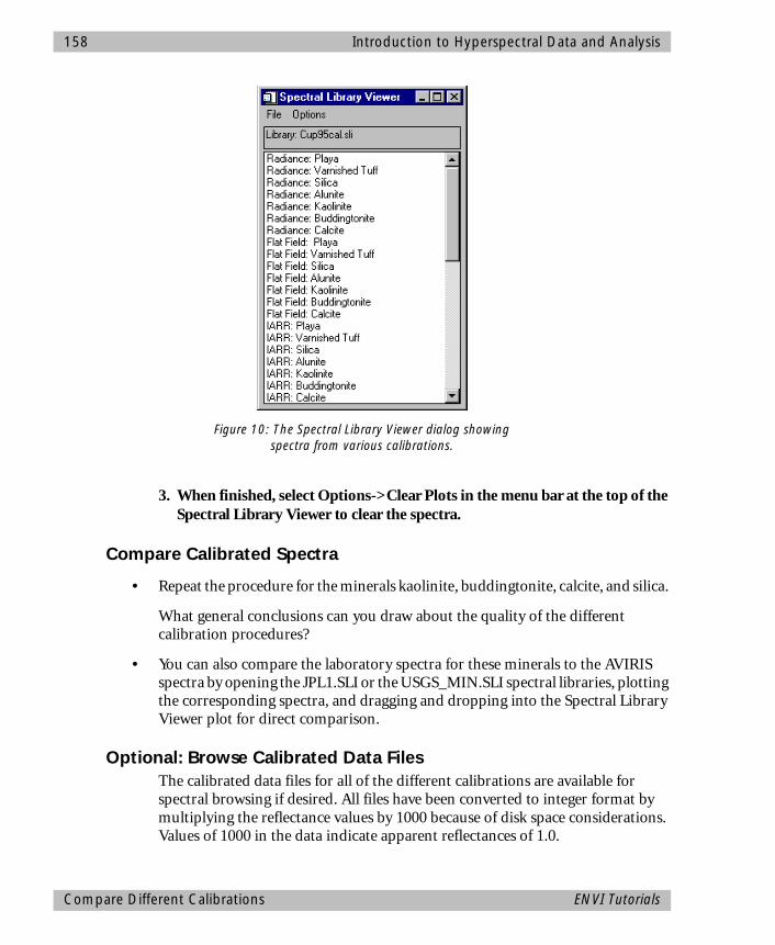
158 Introduction to Hyperspectral Data and Analysis
3. When finished, select Options->Clear Plots in the menu bar at the top of the Spectral Library Viewer to clear the spectra.
Compare Calibrated Spectra
• Repeat the procedure for the minerals kaolinite, buddingtonite, calcite, and silica.
What general conclusions can you draw about the quality of the different calibration procedures?
• You can also compare the laboratory spectra for these minerals to the AVIRIS spectra by opening the JPL1.SLI or the USGS_MIN.SLI spectral libraries, plotting the corresponding spectra, and dragging and dropping into the Spectral Library Viewer plot for direct comparison.
Optional: Browse Calibrated Data FilesThe calibrated data files for all of the different calibrations are available for spectral browsing if desired. All files have been converted to integer format by multiplying the reflectance values by 1000 because of disk space considerations. Values of 1000 in the data indicate apparent reflectances of 1.0.
Figure 10: The Spectral Library Viewer dialog showing spectra from various calibrations.
Compare Different Calibrations ENVI Tutorials
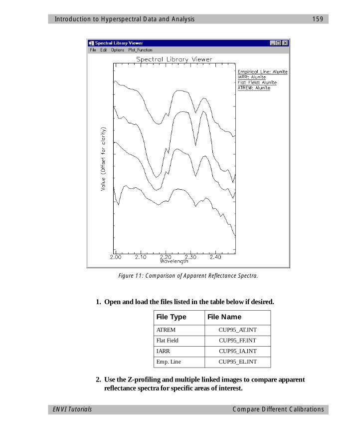
Introduction to Hyperspectral Data and Analysis 159
1. Open and load the files listed in the table below if desired.
2. Use the Z-profiling and multiple linked images to compare apparent reflectance spectra for specific areas of interest.
File Type File Name
ATREM CUP95_AT.INT
Flat Field CUP95_FF.INT
IARR CUP95_IA.INT
Emp. Line CUP95_EL.INT
Figure 11: Comparison of Apparent Reflectance Spectra.
ENVI Tutorials Compare Different Calibrations
160 Introduction to Hyperspectral Data and Analysis
1. After comparison of all of the calibration methods for a variety of minerals, which calibration method(s) best reproduce(s) the laboratory spectra for all minerals? Is there one best calibration method
Exit ENVI
• When you have finished your ENVI session, click “Quit” or “Exit” on the ENVI Main Menu, then type exit at the IDL command prompt.
If you are using ENVI RT, quitting ENVI will take you back to your operating system.
ReferencesConel, J. E., Green, R. O., Vane, G., Bruegge, C. J., Alley, R. E., and Curtiss, B., J., 1987, Airborne imaging spectrometer-2: radiometric spectral characteristics and comparison of ways to compensate for the atmosphere: in Proceedings, SPIE, v. 834, p. 140 - 157.
CSES (Center for the Study of Earth from Space), 1992, ATmospheric REMoval Program (ATREM), version 1.1, University of Colorado, Boulder, 24 p.
Gao, B. C., and Goetz, A. F. H., 1990, Column atmospheric water vapor and vegetation liquid water retrievals from airborne imaging spectrometer data: Journal of Geophysical Research, v. 95, no. D4, p. 3549-3564.
Goetz, A. F. H., Vane, G., Solomon, J. E., and Rock, B. N., 1985, Imaging spectrometry for Earth remote sensing: Science, v. 211, p. 1147 - 1153.
Goetz, A. F. H., and Srivastava, V., 1985, Mineralogical mapping in the Cuprite Mining District, Nevada: in Proceedings of the Airborne Imaging Spectrometer Data Analysis Workshop, JPL Publication 85-41, Jet Propulsion Laboratory, Pasadena, CA, p. 22-29.
Kruse F. A., Raines, G. l., and Watson, K., 1985, Analytical techniques for extracting geologic information from multichannel airborne spectroradiometer and airborne imaging spectrometer data: in Proceedings, 4th Thematic Conference on Remote Sensing for Exploration Geology, Environmental Research Institute of Michigan (ERIM), Ann Arbor, p. 309 - 324.
Kruse, F. A., 1988, use of Airborne Imaging Spectrometer data to map minerals associated with hydrothermally altered rocks in the northern Grapevine Mountains, Nevada and California: Remote Sensing of Environment, v. 24, no. 1, p. 31 - 51.
References ENVI Tutorials

Introduction to Hyperspectral Data and Analysis 161
Kruse, F. A., Kierein-Young, K. S., and Boardman, J. W., 1990, Mineral mapping at Cuprite, Nevada with a 63 channel imaging spectrometer: Photogrammetric Engineering and Remote Sensing, v. 56, no. 1, p. 83-92.
Roberts, D. A., Yamaguchi, Y., and Lyon, R. J. P., 1985, Calibration of Airborne Imaging Spectrometer data to percent reflectance using field measurements: in Proceedings, Nineteenth International Symposium on Remote Sensing of Environment, Ann Arbor, MI, October 21-25, 1985.
Roberts, D. A., Yamaguchi, Y., and Lyon, R. J. P., 1986, Comparison of various techniques for calibration of AIS data: in Proceedings, 2nd AIS workshop, JPL Publication 86-35, Jet Propulsion Laboratory, Pasadena, CA, p. 21-30.
Vane, Gregg, and Goetz, 1985, Introduction to the proceedings of the Airborne Imaging Spectrometer (AIS) data analysis workshop: in Proceedings of the Airborne Imaging Spectrometer Data Analysis Workshop, JPL Publication 85-41, Jet Propulsion Laboratory, Pasadena, CA p. 1 - 21.
ENVI Tutorials References

162 Introduction to Hyperspectral Data and Analysis
References ENVI Tutorials
ENVI Tutorial #8
Basic Hyperspectral Analysis
The following topics are covered in this tutorial:
Overview of This Tutorial ......................................................................................164Spectral Libraries, Image Reflectance Spectra, ROIs, and Color Composites...........1652-D Scatterplots ....................................................................................................173References ............................................................................................................177
163
164 Basic Hyperspectral Analysis
Overview of This TutorialThis tutorial is designed to introduce you to the concepts of Spectral Libraries, Region of Interest (ROI) extraction of spectra, Directed Color composites, and to the use of 2-D scatterplots for simple classification. We will use 1995 Airborne Visible/Infrared Imaging Spectrometer (AVIRIS) apparent reflectance data of Cuprite, Nevada, USA, calibrated using the ATREM atmospheric modeling software. The subsetted data cover the 1.99 to 2.48 µm range in 50 spectral bands approximately 10 nm wide. You will extract ROIs for specific minerals, compare them to library spectra, and design R, G, B color composites to best display the spectral information. You will also use 2-D scatterplots to locate unique pixels, interrogate the data distribution, and perform simple classification. This tutorial is designed to be completed in two to four hours.
Files Used in This TutorialYou must have the ENVI TUTORIALS & DATA CD-ROM mounted on your system to access the files usedby this tutorial, or copy the files to your disk.
The files used in this tutorial are contained in the C95AVSUB subdirectory of the ENVIDATA directory on the ENVI TUTORIALS & DATA CD-ROM.
The files listed below, along with their associated .hdr files, are required to run this exercise. Selected data files have been converted from floating-point to integer format by multiplying by 1000 to conserve disk space. Data values of 1000 represent apparent reflectances of 1.0.
Required FilesCUP95_AT.INT Cuprite ATREM calibrated reflectance data. 50
bands (integer).
JPL1.SLI JPL Spectral Library in ENVI format.
USGS_MIN.SLI USGS Spectral Library in ENVI format.
CUP95_AV.ROI Saved ROI locations.
Topics Covered in This Tutorial
Spectral Libraries, Image Reflectance Spectra, Regions of Interest (ROIs), and Color Composites• Start ENVI and Load AVIRIS
data• Display a Grayscale Image• Browse Image Spectra and
Compare to Spectral Library• Define Regions of Interest
(ROI)• Design Color Images to
Discriminate Mineralogy
2-D Scatterplots as Quick Classifiers• Display Band• Scatterplot Band Selection• Density Slice Scatterplot• Scatterplot Dancing Pixels• Image Dancing Pixels• Scatterplot ROIs• Image ROIs
Overview of This Tutorial ENVI Tutorials
Basic Hyperspectral Analysis 165
Spectral Libraries, Image Reflectance Spectra, ROIs, and Color Composites
This portion of the tutorial is designed to familiarize you with Spectral Libraries, Browsing and extraction of image reflectance spectra, Region of Interest (ROI) definition in ENVI, and directed design of color composite images for spectral discrimination.
Start ENVI and Load AVIRIS dataBefore attempting to start the program, ensure that ENVI is properly installed as described in the installation guide.
♦ To open ENVI in Unix, enter “envi” at the UNIX command line.
♦ To open ENVI from a Windows or Macintosh system, double-click on the ENVI icon.
The ENVI Main Menu appears when the program has successfully loaded and executed.
1. On the ENVI Main Menu, select File->Open Image File and navigate to the C95AVSUB subdirectory of the ENVIDATA directory on the ENVI TUTORIALS & DATA CD-ROM.
2. Choose CUP95_AT.INT as the input file name. The Available Bands List dialog will appear, listing the 50 spectral band names.
Display a Grayscale Image1. Use the scroll bar on the right side of the Available Bands List dialog to scroll
through the list until Band 193 (2.20 µm) is displayed.
2. Click on Band 193 and click “Load” at the bottom of the dialog.
An ENVI image display containing the selected band will appear.
3. Click the right mouse button in the Main Image window and select Functions->Profiles->Z Profile to extract an apparent reflectance spectrum.
Browse Image Spectra and Compare to Spectral Library1. Move the Zoom Window indicator box around the image to browse through
image apparent reflectance spectra.
2. Drag the box by grabbing and dragging with the left mouse button or click the middle mouse button in the Main Image display to center the Zoom Indicator box on the selected pixel.
ENVI Tutorials Spectral Libraries, Image Reflectance Spectra, ROIs, and Color Composites

166 Basic Hyperspectral Analysis
3. Position the Zoom Indicator box at various locations in the image and examine the spectra.
4. Compare apparent reflectance spectra from the image to selected library reflectance spectra.
ENVI includes several spectral libraries. For the purposes of this exercise, you will use the JPL Spectral Library (Groves et al., 1992) and the USGS Spectral Library (Clarke et al., 1993).
5. Select Spectral Tools->Spectral Libraries->Spectral Library Viewer.
6. When the Spectral Library Input File dialog appears, click “Open New File”, select JPL1.SLI from the list, and click “OK”.
JPL1.SLI now appears in the “Select Input File” field of the dialog.
7. Click on the file name and click “OK” to open the Spectral Library Viewer dialog.
8. Select Options->Edit (x, y) Scale Factors and enter a value of 1000 into Y Data Multiplier to match the image apparent reflectance range (0 - 1000).
9. Plot the following spectra in the Spectral Library Viewer window (Figure 1) by clicking on the appropriate mineral name in the list of spectra:
• ALUNITE SO-4A
• BUDDINGTONITE FELDS TS-11A
• CALCITE C-3D
• KAOLINITE WELL ORDERED PS-1A
10.Move the Zoom Indicator Box (which is centered on the “current pixel”) to several different areas in the image and visually compare the image and laboratory spectra.
11.Select Functions->Interactive Analysis->Pixel Locator in the Main Image display and use it to center the Zoom Indicator on pixel 590, 570 (Stonewall Playa).
12.Enter the desired pixel location in the Pixel Locator dialog and click “Apply” to move to that location, which can be used as a starting point for analysis.
13.Now start a new plot window by selecting File->New Window->Inherit in the #1 Spectral Profile window.
Spectral Libraries, Image Reflectance Spectra, ROIs, and Color Composites ENVI Tutorials
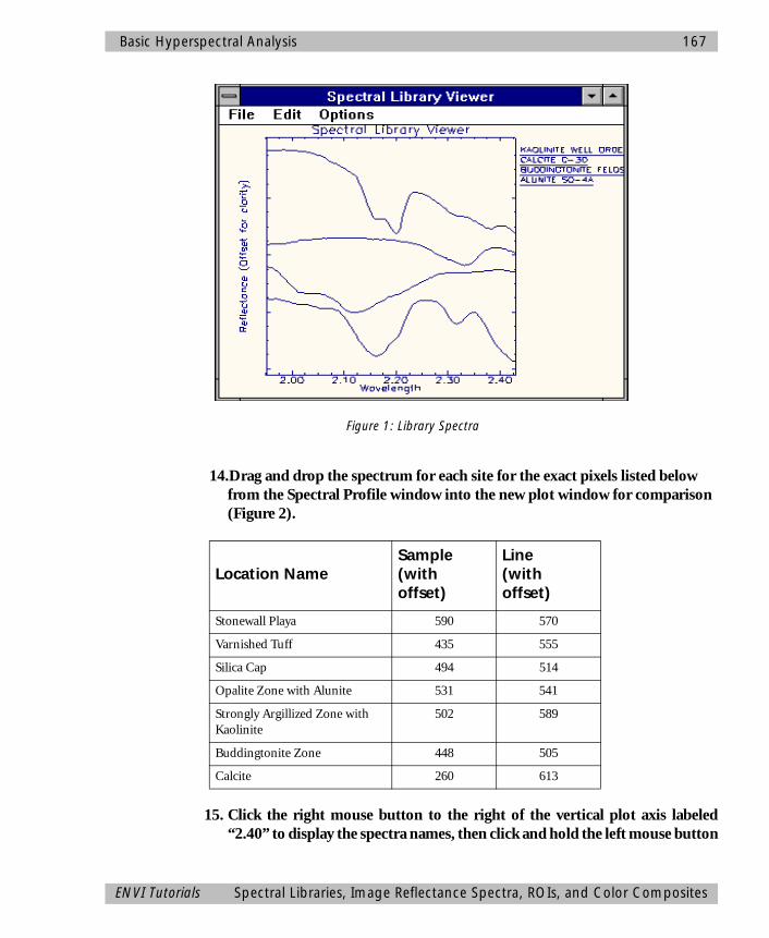
Basic Hyperspectral Analysis 167
14.Drag and drop the spectrum for each site for the exact pixels listed below from the Spectral Profile window into the new plot window for comparison (Figure 2).
15. Click the right mouse button to the right of the vertical plot axis labeled“2.40” to display the spectra names, then click and hold the left mouse button
Location NameSample(with offset)
Line(with offset)
Stonewall Playa 590 570
Varnished Tuff 435 555
Silica Cap 494 514
Opalite Zone with Alunite 531 541
Strongly Argillized Zone with Kaolinite
502 589
Buddingtonite Zone 448 505
Calcite 260 613
Figure 1: Library Spectra
ENVI Tutorials Spectral Libraries, Image Reflectance Spectra, ROIs, and Color Composites
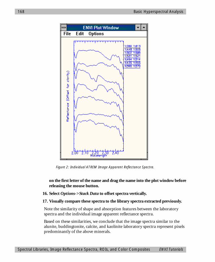
168 Basic Hyperspectral Analysis
on the first letter of the name and drag the name into the plot window beforereleasing the mouse button.
16. Select Options->Stack Data to offset spectra vertically.
17. Visually compare these spectra to the library spectra extracted previously.
Note the similarity of shape and absorption features between the laboratory spectra and the individual image apparent reflectance spectra.
Based on these similarities, we conclude that the image spectra similar to the alunite, buddingtonite, calcite, and kaolinite laboratory spectra represent pixels predominantly of the above minerals.
Figure 2: Individual ATREM Image Apparent Reflectance Spectra.
Spectral Libraries, Image Reflectance Spectra, ROIs, and Color Composites ENVI Tutorials

Basic Hyperspectral Analysis 169
18. Drag and drop spectra from the Spectral Library Viewer into the Z-Profilewindow for direct comparison using the method described above.
19. When you have identified several minerals, continue with the next section.
• Optionally, compare spectra from the USGS Spectral Library USGS_MIN.SLI with image spectra and the JPL Spectral library.
Close Windows and Plots
• To close all of the previous plot windows, select Basic Tools->Display Controls->Close All Plot Windows.
• To close these dialogs, select File->Cancel in the Spectral Library Viewer dialog and the Pixel Locator.
Define Regions of InterestRegions of Interest (ROIs) are used to extract statistics and average spectra from groups of pixels. You can define as many ROIs as you wish in any displayed image.
1. Select Basic Tools->Region of Interest->Define Region of Interest.
2. When the Region of Interest Controls dialog appears (Figure 3). click in the “Display #” text box at the top of the dialog, and enter “1” for the display number.
Create New Region of InterestTo begin drawing an ROI:
1. Click the left mouse button in the image.
2. Draw the ROI by clicking the left mouse button at the axes of a polygon, or draw continuously by clicking and dragging the left mouse button.
3. Complete the ROI by clicking the right mouse button to close the polygon.
4. Click on the Stats button to calculate the statistics and plot a mean spectrum (white), the first standard deviation above and below the mean spectrum (green), and the Min/Max envelope containing all of the spectra in the ROI (red).
5. Click “Cancel” in the File Statistics Report and select File->Cancel in the Avg Spectrum plot to close the dialog and plot respectively.
6. Click “Delete” in the Region of Interest Controls dialog to delete the selected ROI.
ENVI Tutorials Spectral Libraries, Image Reflectance Spectra, ROIs, and Color Composites
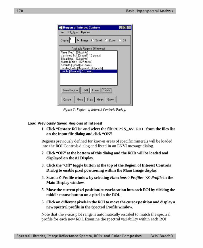
170 Basic Hyperspectral Analysis
Load Previously Saved Regions of Interest1. Click “Restore ROIs” and select the file CUP95_AV.ROI from the files list
on the input file dialog and click “OK”.
Regions previously defined for known areas of specific minerals will be loaded into the ROI Controls dialog and listed in an ENVI message dialog.
2. Click “OK” at the bottom of this dialog and the ROIs will be loaded and displayed on the #1 Display.
3. Click the “Off” toggle button at the top of the Region of Interest Controls Dialog to enable pixel positioning within the Main Image display.
4. Start a Z-Profile window by selecting Functions->Profiles->Z-Profile in the Main Display window.
5. Move the current pixel position/cursor location into each ROI by clicking the middle mouse button on a pixel in the ROI.
6. Click on different pixels in the ROI to move the cursor position and display a new spectral profile in the Spectral Profile window.
Note that the y-axis plot range is automatically rescaled to match the spectral profile for each new ROI. Examine the spectral variability within each ROI.
Figure 3: Region of Interest Controls Dialog.
Spectral Libraries, Image Reflectance Spectra, ROIs, and Color Composites ENVI Tutorials

Basic Hyperspectral Analysis 171
Extract Mean Spectra from ROIs1. Select a ROI name in the Region of Interest Controls dialog by clicking on the
name, then click “Stats” to extract statistics and a spectral plot of the selected ROI.
2. Examine the spectral variability of each ROI by comparing the mean spectrum (white) with the 1st standard deviation spectra (green above and below the mean) and the envelope spectra (red above and below the mean).
3. Repeat for each ROI.
• If you wish, load the corresponding library signatures from the JPL1.SLI library into the plot window for direct comparison/identification.
Don’t forget to use a “Y-Scaling Factor” of 1000 when loading the library spectra.
4. When you have finished, click “Cancel” in each of the File Statistics Report dialogs.
5. Select File->Cancel in each plot window to remove these plots from the screen.
6. Click “Mean All” in the Region of Interest Controls dialog to plot the average spectrum for each ROI in a single plot window (Figure 4).
7. Compare the spectral features of each spectrum and note unique characteristics that might allow identification.
8. Select Options->Stack Data to offset spectra for comparison.
• If desired, load the corresponding spectral library signatures from the JPL1.SLI library for direct comparison of image apparent reflectance spectra with laboratory spectra.
Don’t forget to use a Y Factor of 1000 when loading the library spectra.
• Optionally, compare spectra from the USGS Spectral Library USGS_MIN.SLI with image spectra and the JPL Spectral library.
Optional: Define New ROIsTo define a new ROI:
1. Click on the “Image” toggle button in the Region of Interest Controls dialog and click “New Region”.
2. Enter a name in the “Name:” text box and change the ROI color by choosing a color from the pulldown list of colors to the right of the “Name” field.
ENVI Tutorials Spectral Libraries, Image Reflectance Spectra, ROIs, and Color Composites
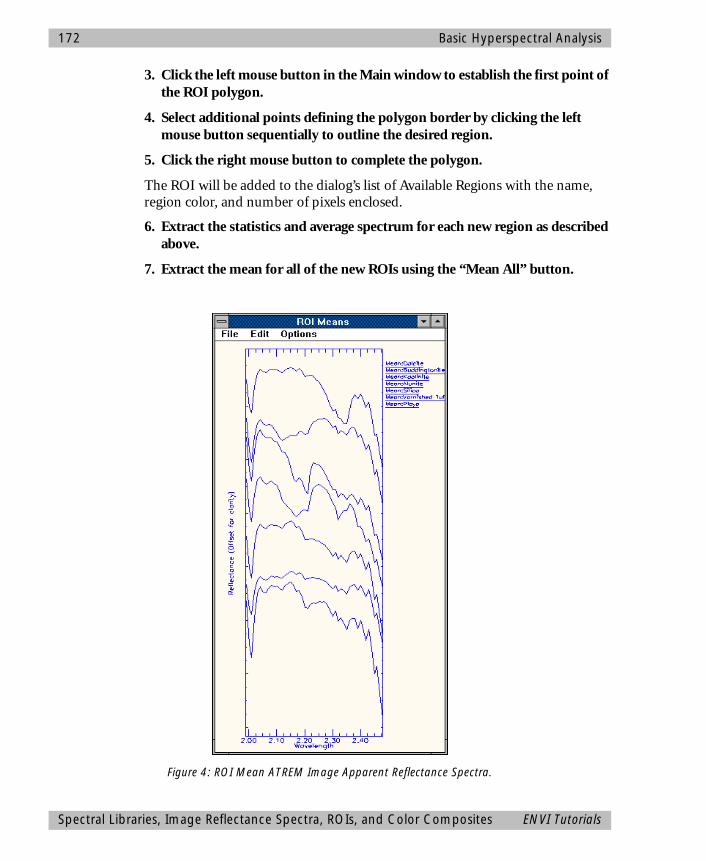
172 Basic Hyperspectral Analysis
3. Click the left mouse button in the Main window to establish the first point of the ROI polygon.
4. Select additional points defining the polygon border by clicking the left mouse button sequentially to outline the desired region.
5. Click the right mouse button to complete the polygon.
The ROI will be added to the dialog’s list of Available Regions with the name, region color, and number of pixels enclosed.
6. Extract the statistics and average spectrum for each new region as described above.
7. Extract the mean for all of the new ROIs using the “Mean All” button.
Figure 4: ROI Mean ATREM Image Apparent Reflectance Spectra.
Spectral Libraries, Image Reflectance Spectra, ROIs, and Color Composites ENVI Tutorials

Basic Hyperspectral Analysis 173
Design Color Images to Discriminate Mineralogy1. Load a color composite image by clicking on the “RGB Color” toggle button
in the Available Bands List and clicking sequentially on Band 183, Band 193, and Band 207.
2. Click “Load RGB” to load the color image into the current image display.
Note that the positions of the bands used to make the RGB color composite image are marked in the Z-Profile with vertical red, green, and blue lines.
3. Click on the “Off” toggle button in the Region of Interest Controls dialog and use the Z profiler to browse spectra at or near your ROI locations from above.
Note where the selected RGB bands fall with respect to spectral features in the previously displayed mean spectra and how the spectral features affect the color observed in the image. After inspecting a few sites, you should begin to understand how the color composite colors correspond with the spectral signature. For instance, the alunitic regions appear magenta in the RGB composite because the green band is within the alunite absorption feature, giving a low green value, while the red and blue bands are of almost equal reflectance. The combination of red and blue results in a magenta color for pixels containing alunite.
• Based on the above results, try these exercises:
1. Predict how certain spectra will look, given a particular pixel’s color in the RGB image.
2. Explain the colors of the training sites, in terms of their spectral features.
3. Design and test specific RGB band selections that maximize your ability to map certain minerals, like kaolinite and calcite.
Close Plot Windows and ROI Controls
• To close all open plot windows, select Basic Tools->Display Controls->Close All Plot Windows.
• To close the Region of Interest Control dialog, click “Cancel”.
2-D Scatterplots
Examine 2-D Scatterplots1. Start a 2-d scatterplot for the apparent reflectance image by selecting
Functions->Interactive Analysis->2-D Scatter Plots in the Main window.
ENVI Tutorials 2-D Scatterplots
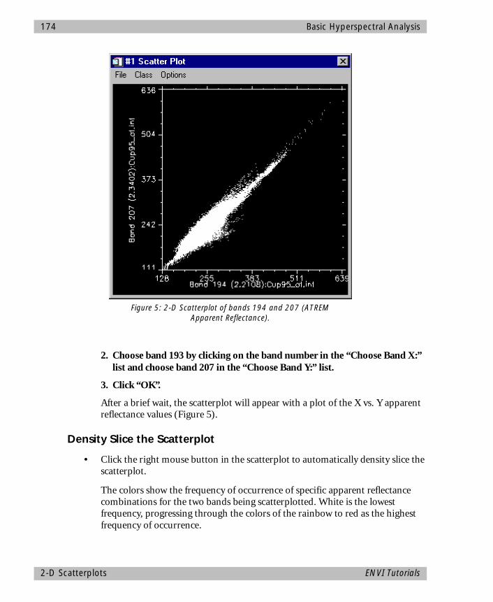
174 Basic Hyperspectral Analysis
2. Choose band 193 by clicking on the band number in the “Choose Band X:” list and choose band 207 in the “Choose Band Y:” list.
3. Click “OK”.
After a brief wait, the scatterplot will appear with a plot of the X vs. Y apparent reflectance values (Figure 5).
Density Slice the Scatterplot
• Click the right mouse button in the scatterplot to automatically density slice the scatterplot.
The colors show the frequency of occurrence of specific apparent reflectance combinations for the two bands being scatterplotted. White is the lowest frequency, progressing through the colors of the rainbow to red as the highest frequency of occurrence.
Figure 5: 2-D Scatterplot of bands 194 and 207 (ATREM Apparent Reflectance).
2-D Scatterplots ENVI Tutorials
Basic Hyperspectral Analysis 175
Scatterplot Dancing Pixels1. Click and drag the left mouse button in the Main Image window to toggle
“Dancing Pixels” in the scatterplot.
The red pixels in the scatterplot correspond to those pixels within a 10 x 10 box around the cursor in the Main Image window.
• You can change the box-cursor size by selecting Options->Set Patch Size in the scatter plot window.
2. Move the cursor in the Main window with the left mouse button depressed to cause the red-highlighted pixels to change in the scatterplot display.
3. Try to predict the locations of certain image colors in the scatterplot, then check them.
Notice the shape of the red sub-scatterplot of dancing pixels.
4. Try changing the patch size and observe the difference.
Image Dancing Pixels1. Click and drag the center mouse button in the scatterplot window over any
portion of the white scatterplot to toggle “Dancing Pixels” in the Main Image window.
The red pixels in the image correspond to those pixels within a 10 x 10 box around the cursor in the scatterplot window.
• You can change the box-cursor size by selecting Options->Set Patch Size in the scatter plot window.
2. Move the cursor around the scatterplot with the middle mouse button depressed to cause the red-highlighted pixels to change in the Main Image display.
Note the spatial distribution and coherency of the selected pixels.
3. Try changing the patch size and observe the difference.
Scatterplot ROIsThe scatterplot tool can also be used as a quick classifier.
1. Click the left mouse button in the scatterplot to select the first point of a Region of Interest (ROI).
2. Draw a ROI polygon in the scatter plot by selecting the desired line segments using the left mouse button.
ENVI Tutorials 2-D Scatterplots

176 Basic Hyperspectral Analysis
3. Click the right mouse button to close the polygon.
Image pixels with the two-band characteristics outlined by the polygon will be color-coded red in the Main Image window.
4. Choose another color from the Class pulldown menu in the scatterplot window.
5. Draw another polygon and the corresponding pixels will be highlighted in the selected color on the image.
• If you want to remove a class, select Options->Clear Class.
• You can also clear the current class by clicking using the middle mouse but-ton outside (below) the plot axes.
6. Use the 2-D scatterplot tool to work backwards from the scatterplot to see where certain pixels occur in the image.
• Classes can be converted to ROIs to act as training sets for classification using all of the bands by selecting Options->Export Class or Export All from the scatterplot menu bar.
ROIs exported in this fashion will appear in the Region of Interest Controls dialog and be available for subsequent supervised classification.
7. Select Options->Clear All in the scatterplot to clear both scatterplot and image.
Image ROIsThe scatter plot tool also functions as a simple classifier from the image.
1. Choose Options->Image ROI in the scatterplot.
2. Draw polygons in the Main Image window (as before, click the left mouse button to draw lines and the right button to close the polygon).
They will be mapped to the scatterplot and highlighted in the currently selected color. After the pixels are highlighted on the scatterplot, all of the matching pixels in the image will be inverse mapped to the Main Image window and highlighted in the same color, as though you had drawn the scatterplot region yourself. This is the simplest form of 2-band classification, but it is still a powerful tool.
3. Draw a few image regions and note the correspondence between image color and scatterplot characteristics.
2-D Scatterplots ENVI Tutorials
Basic Hyperspectral Analysis 177
Scatterplots and Spectral Mixing
• Can you explain the overall diagonal shape of the scatterplot in terms of spectral mixing? Where do the purest pixels in the image fall on the scatterplot? Are there any secondary “projections” or “points” on the scatterplot?
1. Choose some other band combinations for scatterplotting by selecting Options->Change Bands in the scatterplot.
Try at least one pair of adjacent bands and other pairs that are far apart spectrally.
• How do the scatterplots change shape with different band combinations? Can you describe the n-Dimensional “shape” of the data cloud?
2. Close the scatterplot window when finished by selecting File->Cancel in the scatterplot.
Close the Scatterplot
• To close the scatterplot window, select File->Cancel in the scatterplot menu bar.
Close Files and Exit ENVI.
• When you have finished your ENVI session, click “Quit” or “Exit” on the ENVI Main Menu, then type exit at the IDL command prompt.
If you are using ENVI RT, quitting ENVI will take you back to your operating system.
ReferencesClark, R. N., Swayze, G. A., Gallagher, A., King, T. V. V., and Calvin, W. M., 1993, The U. S. Geological Survey Digital Spectral Library: Version 1: 0.2 to 3.0 mm: U. S. Geological Survey, Open File Report 93-592, 1340 p.
Grove, C. I., Hook, S. J., and Paylor, E. D., 1992, Laboratory reflectance spectra of 160 minerals, 0.4 to 2.5 Micrometers: JPL Publication 92-2.
ENVI Tutorials References

178 Basic Hyperspectral Analysis
References ENVI Tutorials
ENVI Tutorial #9
Selected Mapping Methods Using Hyperspectral Data
The following topics are covered in this tutorial:
Overview of This Tutorial ......................................................................................180Removal of Residual Calibration Errors using “Effort” ............................................181Spectral Angle Mapper Classification.....................................................................184Spectral Feature Fitting (SFF) and Analysis.............................................................193References ............................................................................................................201
179
180 Selected Mapping Methods Using Hyperspectral Data
Overview of This TutorialThis tutorial is designed to introduce you to advanced concepts and procedures for analysis of imaging spectrometer data or hyperspectral images. We will use 1995 Airborne Visible/Infrared Imaging Spectrometer (AVIRIS) data from Cuprite, Nevada, to investigate the unique properties of hyperspectral data and how spectral information can be used to identify mineralogy. We will evaluate “Effort” “polished” spectra vs ATREM-calibrated data, and review the Spectral Angle Mapper classification. We will compare apparent reflectance spectra and continuum-removed spectra. We will also compare apparent reflectance images and continuum-removed images and evaluate Spectral Feature Fitting results. This tutorial is designed to be completed in two to four hours.
Files Used in This TutorialYou must have the ENVI TUTORIALS & DATACD-ROM mounted on your system to accessthe files used by this tutorial, or copy the filesto your disk.
The files used in this tutorial are contained in the C95AVSUB subdirectory of the ENVIDATA directory on the ENVI TUTORIALS & DATA CD-ROM.
The files listed below, along with their associated .hdr files, are required to run this exercise. Optional files listed below may also be used if more detailed calibration comparisons are desired.
All image data files have been converted to integer format by multiplying the reflectance values by 1000 because of disk space considerations. A value of 1000 therefore represents apparent reflectance of 1.0.
Required FilesCUP95_AT.INT Cuprite ATREM calibrated apparent reflectance
data. 50 bands (integer).
CUP95EFF.INT Cuprite Effort-Corrected ATREM calibrated ap-parent reflectance data. 50 bands (integer).
Topics Covered in This Tutorial
Removal of Residual Calibration Errors from Apparent Reflectance Data• Comparison of ATREM and
“EFFORT” corrected data
Spectral Angle Mapper Classification• Select Image Endmembers• Select Spectral Library Endmembers• Review SAM Classification Results• Optional: Generate New Sam
Classified Images using the “Rule Classifier”
Continuum Removal and Spectral Feature Fitting• Continuum Removal for individual
spectra and comparison to apparent reflectance spectra
• Comparison of apparent reflectance images and continuum-removed images
• Spectral Feature Fitting Background• Comparison of Scale and RMS Images• 2-D Scatterplots of SFF Scale and
RMS Result Images• Mineral Mapping with “Fit” images
Overview of This Tutorial ENVI Tutorials
Selected Mapping Methods Using Hyperspectral Data 181
JPL1.SLI JPL Spectral Library in ENVI format.
USGS_MIN.SLI USGS Spectral Library in ENVI format.
CUP95_AV.ROI Saved ROI locations.
CUPSAMEM.ASC Optional file of ROI mean spectra.
CUPSAM1.IMG SAM classification image using ROI image spectra endmembers.
CUPRUL1.IMG SAM rule image using ROI image spectra end-members.
CUPSAM2.IMG SAM classification image using Spectral Li-brary endmembers.
CUPRUL2.IMG SAM rule images using Spectral Library end-members.
CUP95_CR.DAT Continuum-removed data (floating point)
CUP95SFF.DAT Spectral Feature Fitting Results
CUP95SFR.DAT Spectral Feature Fitting Band-Math Results
Removal of Residual Calibration Errors using “Effort”“Effort”, the “Empirical Flat Field Optimized Reflectance Transformation” is a correction used to remove residual “saw-tooth” instrument (or calibration-introduced) noise and atmospheric effects from ATREM-calibrated AVIRIS data. While this correction is not currently available in ENVI, it is the type of custom correction that might be designed for specific data sets to improve overall quality of spectra. It provides the best reflectance spectra available from AVIRIS data, so the Effort data are used in later exercises in this tutorial. Effort is a relatively automated improvement on the Flat-Field Calibration method (Boardman, 1996). The Effort correction selects those AVIRIS spectra that match a low order polynomial estimate in a least-squares sense as representative featureless spectra. These spectra are averaged and a mild gain factor is determined to remove systematic, coherent noise, present in every spectrum, including small residual atmospheric effects near 2.0 µm range attributable to CO2. We will compare 1995 AVIRIS data calibrated to reflectance using ATREM and the corresponding Effort-corrected ATREM data.
Open and Load the 1995 Effort-Corrected Data1. Open the file CUP95EFF.INT by selecting File->Open Image File from the ENVI Main Menu.
1. This is the 1995 AVIRIS ATREM-calibrated apparent reflectance data with the Effort correction applied.
ENVI Tutorials Removal of Residual Calibration Errors using “Effort”

182 Selected Mapping Methods Using Hyperspectral Data
2. Start a new display by clicking on the “New” button in the Available Bands List.
3. Load band 193 (2.20 µm) as a grayscale image in the new image display by clicking “Load Band”.
4. Start a Z-Profile by clicking the right mouse button in the Main Image display and selecting Functions->Profiles->Z-Profile.
5. Move the profile to the bottom of the screen for comparison with the 1995 ATREM data.
Compare ATREM and Effort Spectra1. Click the right mouse button in the Effort Main Image display and select
Functions->Link->Link Display.
2. Click “OK” in the Link Display dialog to activate the link.
3. Select Functions->Link->Dynamic Overlay Off to enable normal mouse interaction in the Effort Main Display window.
Moving the Zoom Window indicator box in this image will cause the cursor location to be updated in the ATREM Main Display window. Both spectral profiles will show the spectrum for the current pixel.
4. Move the Zoom Window indicator box around the image and compare the corresponding ATREM and Effort spectra. Note where the major differences occur.
5. Now position the cursor at 503, 581 by selecting Functions->Interactive Analysis->Pixel Locator in the Main Display window.
6. Compare the Effort-corrected spectrum to the ATREM-only spectrum (Figure 1).
7. Drag and drop the Effort spectrum into the plot with the ATREM-only spectrum by clicking with the right mouse button to the right of the plot axis to display the name, grabbing the first character of the name and dragging with the left mouse button, and releasing in the ATREM-only plot window.
8. Change the color of the Effort spectrum by selecting Edit->Data Parameters” in the Plot Window menu bar.
• Stack the spectra if desired by selecting Options->Stack Data.
Note how similar the two spectra are, but how very small coherent noise “wiggles” have been removed from the Effort spectrum. Also note the correction of residual CO2 at 2.01 µm.
Removal of Residual Calibration Errors using “Effort” ENVI Tutorials
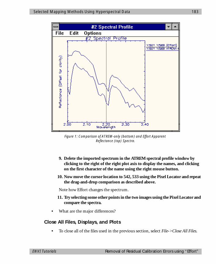
Selected Mapping Methods Using Hyperspectral Data 183
9. Delete the imported spectrum in the ATREM spectral profile window by clicking to the right of the right plot axis to display the names, and clicking on the first character of the name using the right mouse button.
10. Now move the cursor location to 542, 533 using the Pixel Locator and repeat the drag-and-drop comparison as described above.
Note how Effort changes the spectrum.
11. Try selecting some other points in the two images using the Pixel Locator and compare the spectra.
• What are the major differences?
Close All Files, Displays, and Plots
• To close all of the files used in the previous section, select File->Close All Files.
Figure 1: Comparison of ATREM-only (bottom) and Effort Apparent Reflectance (top) Spectra.
ENVI Tutorials Removal of Residual Calibration Errors using “Effort”
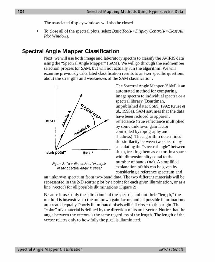
184 Selected Mapping Methods Using Hyperspectral Data
The associated display windows will also be closed.
• To close all of the spectral plots, select Basic Tools->Display Controls->Close All Plot Windows.
Spectral Angle Mapper ClassificationNext, we will use both image and laboratory spectra to classify the AVIRIS data using the “Spectral Angle Mapper” (SAM). We will go through the endmember selection process for SAM, but will not actually run the algorithm. We will examine previously calculated classification results to answer specific questions about the strengths and weaknesses of the SAM classification.
The Spectral Angle Mapper (SAM) is an automated method for comparing image spectra to individual spectra or a spectral library (Boardman, unpublished data; CSES, 1992; Kruse et al., 1993a). SAM assumes that the data have been reduced to apparent reflectance (true reflectance multiplied by some unknown gain factor controlled by topography and shadows). The algorithm determines the similarity between two spectra by calculating the “spectral angle” between them, treating them as vectors in a space with dimensionality equal to the number of bands (nb). A simplified explanation of this can be given by considering a reference spectrum and
an unknown spectrum from two-band data. The two different materials will be represented in the 2-D scatter plot by a point for each given illumination, or as a line (vector) for all possible illuminations (Figure 2).
Because it uses only the “direction” of the spectra, and not their “length,” the method is insensitive to the unknown gain factor, and all possible illuminations are treated equally. Poorly illuminated pixels will fall closer to the origin. The “color” of a material is defined by the direction of its unit vector. Notice that the angle between the vectors is the same regardless of the length. The length of the vector relates only to how fully the pixel is illuminated.
Figure 2: Two-dimensional example of the Spectral Angle Mapper
Spectral Angle Mapper Classification ENVI Tutorials
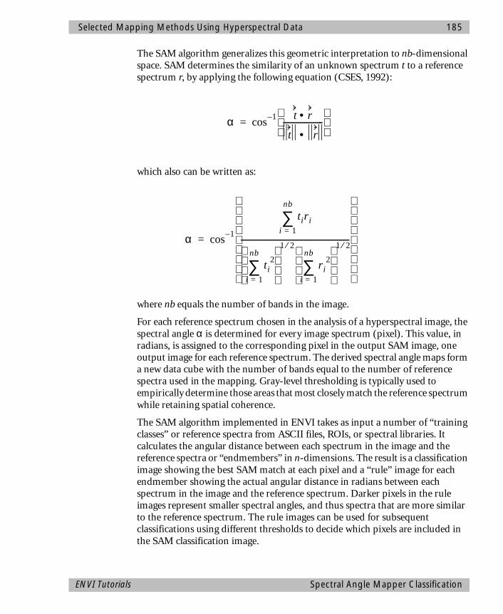
Selected Mapping Methods Using Hyperspectral Data 185
The SAM algorithm generalizes this geometric interpretation to nb-dimensional space. SAM determines the similarity of an unknown spectrum t to a reference spectrum r, by applying the following equation (CSES, 1992):
which also can be written as:
where nb equals the number of bands in the image.
For each reference spectrum chosen in the analysis of a hyperspectral image, the spectral angle α is determined for every image spectrum (pixel). This value, in radians, is assigned to the corresponding pixel in the output SAM image, one output image for each reference spectrum. The derived spectral angle maps form a new data cube with the number of bands equal to the number of reference spectra used in the mapping. Gray-level thresholding is typically used to empirically determine those areas that most closely match the reference spectrum while retaining spatial coherence.
The SAM algorithm implemented in ENVI takes as input a number of “training classes” or reference spectra from ASCII files, ROIs, or spectral libraries. It calculates the angular distance between each spectrum in the image and the reference spectra or “endmembers” in n-dimensions. The result is a classification image showing the best SAM match at each pixel and a “rule” image for each endmember showing the actual angular distance in radians between each spectrum in the image and the reference spectrum. Darker pixels in the rule images represent smaller spectral angles, and thus spectra that are more similar to the reference spectrum. The rule images can be used for subsequent classifications using different thresholds to decide which pixels are included in the SAM classification image.
α cos1– t r•
t r•---------------------
=
α cos1–
tirii 1=
nb
∑
ti2
i 1=
nb
∑ 1 2⁄
ri2
i 1=
nb
∑ 1 2⁄---------------------------------------------------------
=
ENVI Tutorials Spectral Angle Mapper Classification

186 Selected Mapping Methods Using Hyperspectral Data
Select Image Endmembers1. Open the 1995 AVIRIS ATREM-calibrated apparent reflectance data file, CUP95EFF.INT.
2. Load band 193 (2.20 µm) as a grayscale image in the new image display by clicking “Load Band” in the Available Bands List.
3. Start the SAM endmember selection process by selecting Classification->Supervised Classification->Spectral Angle Mapper.
• You may also make this selection from the Spectral Tools Menu.
4. Select the file CUP95EFF.INT as the input file and click “OK”.
5. When the SAM Endmember Collection dialog appears, select Import->from ASCII File.
The Enter ASCII Plot Filename dialog will appear and available files will be listed.
6. Enter “*.asc” in the File Name text box to list all of the ASCII files available.
7. Select the file CUP95_EM.ASC and click “OK” to open the file.
8. When the Input ASCII File dialog appears, deselect spectra 3, 4, 9, and 11 by clicking on the checked boxes to the left of the number spectra.
This will leave you with the mean spectra Zeolite, Calcite, Alunite (2.16), Kaolinite, Illite/Muscovite, Silica (Bright), and Buddingtonite.
9. Click “OK” to load all of the endmember spectra into the SAM Endmember Collection dialog.
10. Plot the endmember spectra by clicking “Plot Endmembers”.
11. Stack the spectra for improved comparison of spectral features (Figure 3) by selecting Options->Stack Data in the plot window.
Normally, you would click “OK” to start the classification, but because classification can take some time, preprocessed results are provided for this exercise.
12. Click “Cancel” and continue by reviewing previously calculated SAM results as described below.
Execute SAM, Resources Permitting1. If sufficient time and resources are available, click “Apply” and enter output
file names in the Spectral Angle Mapper Parameters dialog and click “OK”.
2. Open the SAM classification image by selecting File->Open Image File and choosing CUPSAM1.IMG as the input file name.
Spectral Angle Mapper Classification ENVI Tutorials
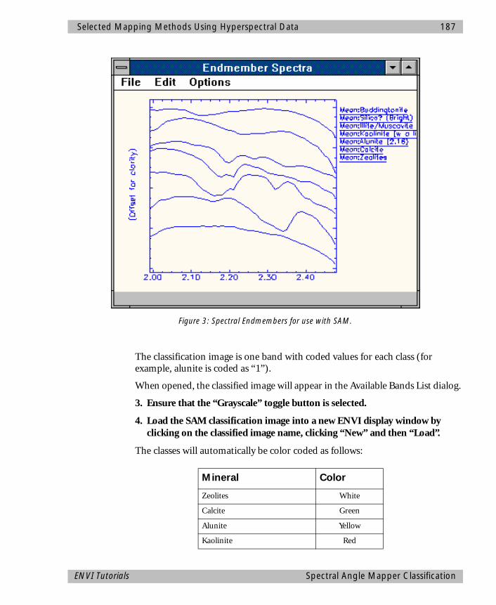
Selected Mapping Methods Using Hyperspectral Data 187
The classification image is one band with coded values for each class (for example, alunite is coded as “1”).
When opened, the classified image will appear in the Available Bands List dialog.
3. Ensure that the “Grayscale” toggle button is selected.
4. Load the SAM classification image into a new ENVI display window by clicking on the classified image name, clicking “New” and then “Load”.
The classes will automatically be color coded as follows:
Mineral Color
Zeolites White
Calcite Green
Alunite Yellow
Kaolinite Red
Figure 3: Spectral Endmembers for use with SAM.
ENVI Tutorials Spectral Angle Mapper Classification

188 Selected Mapping Methods Using Hyperspectral Data
Note The number of pixels displayed as a specific class is a function of the threshold used to generate the classification. Just because a given pixel is classified as a specific mineral doesn’t make it so. SAM is a similarity measure, not an identifier.
5. Open the Effort data by selecting File->Open Image File and choosing the file CUP95EFF.INT.
6. Click on “RGB” Color in the Available Bands List, open a new display by clicking on “New”, and load bands 183, 193, and 207 as an RGB image.
7. Start a spectral profile by selecting Functions->Profiles->Z-Profile in the Main Image display.
8. Compare the SAM classification results with the distributions shown by the color composite image.
9. Compare the actual spectra for classified pixels with the endmember spectra using spectral browsing.
• Use image linking for direct comparison, if desired.
10. Load the SAM rule images for this classification.
11. Open the SAM rule image by selecting File->Open Image File and choosing CUPRUL1.IMG as the input file name.
The rule image has one band for each endmember classified, with the pixel values representing the spectral angle in radians. Lower spectral angles (darker pixels) represent better spectral matches to the endmember spectrum.
When opened, one band for each endmember will appear in the Available Bands List dialog.
12. Ensure that the “Grayscale” toggle button is selected and load a SAM rule image into a third ENVI display window by clicking on the classified image name, clicking “New” and then “Load”.
13. Evaluate the image with respect to the color composite and the SAM classification image as well as the ROI means and individual spectra extracted using the Z Profiler.
14. Select Functions->Color Mapping->ENVI Color Tables in the Main Image.
Illite/Muscovite Dark Green
Silica Blue
Buddingtonite Maroon
Mineral Color
Spectral Angle Mapper Classification ENVI Tutorials

Selected Mapping Methods Using Hyperspectral Data 189
15. Use the “Stretch Bottom” and “Stretch Top” sliders to adjust the SAM rule thresholds to highlight those pixels with the greatest similarity to the selected endmember.
16. Pull the Stretch Bottom slider all the way to the right and the Stretch Top slider all the way to the left to highlight the most similar pixels in white.
17. Move the Stretch Bottom slider gradually to the left to reduce the number of highlighted pixels and show only the best SAM matches in white.
• You may use a rule image color composites or image animation if desired to compare individual rule images.
18. Repeat the process with each SAM rule image.
19. Click “Cancel” when finished to close the ENVI Color Tables dialog.
Select Spectral Library EndmembersIn this exercise we will once again go through the endmember selection process, but we won’t actually perform the SAM classification. Previously saved SAM results will be used for comparisons. If you have time, you can perform your own SAM classification using spectral library endmembers.
1. Open the spectral library if not previously loaded.
2. Select Spectral Tools->Spectral Libraries->Spectral Library Viewer.
3. Click “Open New File”, select the file JPL1SLI.DAT, and click “OK”.
4. Use the Spectral Library Viewer to plot the following spectra in the Spectral Library Viewer window by clicking on the appropriate mineral name in the list of spectra.
• ALUNITE SO-4A
• BUDDINGTONITE FELDS TS-11A
• CALCITE C-3D
• CHABAZITE TS-15A (a zeolite mineral)
• ILLITE PS-11A
• KAOLINITE WELL ORDERED PS-1A
5. Start the SAM endmember selection process by selecting Classification->Supervised Classification->Spectral Angle Mapper.,
You may also access this function from the ENVI Spectral Tools menu.
6. Select the file CUP95EFF.INT as the input file and click “OK”.
ENVI Tutorials Spectral Angle Mapper Classification

190 Selected Mapping Methods Using Hyperspectral Data
7. When the SAM Endmember Collection dialog appears, select Import Spectra->from Spectral Library.
8. Select the file JPLSLI1.DAT and click “OK”.
9. If you haven’t already done so using the Spectral Library Viewer, select the following spectra for the classification from the JPL Spectral Library by clicking on their names in the Spectral Library Input dialog and clicking “OK”:
• ALUNITE SO-4A
• BUDDINGTONITE FELDS TS-11A
• CALCITE C-3D
• CHABAZITE TS-15A (a zeolite mineral)
• ILLITE PS-11A
• KAOLINITE WELL ORDERED PS-1A
10. Open the USGS spectral library.
11. Select Spectral Tools->Spectral Libraries->Spectral Library Viewer.
12. Click “Open New File”, select the file USGS_SLI.DAT and click “OK”.
13. Select the endmember “opal2.spc Opal TM8896 (Hyalite)” from the list of spectra by clicking on the name followed by clicking “OK”.
Note that the spectra are automatically resampled to the AVIRIS wavelengths and resolution using the AVIRIS band positions and FWHM and listed in the Endmember Collection dialog.
14. Click “Plot Endmembers” to plot the endmember spectra for these AVIRIS data.
15. Choose Options->Stack Data in the plot window to offset the spectra vertically for comparison.
16. Compare these spectra to the image spectra plotted in the previous SAM exercise.
17. Since we will not actually be performing the SAM classification because of time constraints, click “Cancel” in the Endmember Collection dialog to continue the exercise.
• If you have time, you can generate your own SAM classification by clicking “OK”.
Spectral Angle Mapper Classification ENVI Tutorials

Selected Mapping Methods Using Hyperspectral Data 191
Review SAM Results1. Open the pre-calculated SAM classification image generated using Spectral
Library Endmembers by selecting File->Open Image File.
2. Select CUPSAM2.IMG as the input file name and click “OK”.
The classification image is one band with coded values for each class (for example, alunite is coded as “1”). When opened, the classified image will appear in the Available Bands List dialog.
3. Ensure that the “Grayscale” toggle button is selected.
4. Load the SAM classification image into a new ENVI display window by clicking on the classified image name, clicking “New” and then “Load”.
The classes will automatically be color coded as follows:
Note The number of pixels displayed as a specific class is a function of the threshold used to generate the classification. Just because a given pixel is classified as a specific mineral doesn’t make it so. SAM is a similarity measure, not an identifier).
5. Compare the classification results with the distributions shown by the color composite image, the previous classification using image spectra, and the library spectra.
• Use image linking for direct comparison if desired.
6. Load the SAM rule images by selecting File->Open Image File and selecting CUPRUL2.IMG as the input file name and clicking “OK”.
Again, the rule image has one band for each endmember classified, with the pixel values representing the spectral angle in radians. Lower spectral angles (darker pixels) represent better spectral matches to the endmember spectrum. When opened, one band for each endmember will appear in the Available Bands List dialog.
Mineral Color
Zeolites White
Calcite Green
Alunite Yellow
Kaolinite Red
Illite/Muscovite Dark Green
Silica Blue
Buddingtonite Maroon
ENVI Tutorials Spectral Angle Mapper Classification

192 Selected Mapping Methods Using Hyperspectral Data
7. Ensure that the “Grayscale” toggle button is selected.
8. Load a SAM rule image into a new ENVI display window by clicking on the classified image name, clicking “New” and then “Load”.
9. Evaluate the image using the ENVI Color Tables as above and with respect to the color composite and the SAM classification image as well as the ROI means and individual spectra extracted using the Z Profiler.
• Also use a rule image color composite or image animation if desired to com-pare individual rule images.
10. Repeat the process with each SAM rule image.
Based upon the results of the two SAM classifications, answer the following questions:
1. What ambiguities exist in the SAM classification based on your images and spectra above?
2. Why are the two classifications so different? What factors could affect how well SAM matches the endmember spectra?
3. How could you determine which thresholds represent a true map of the selected endmem-bers?
4. Can you see the topographic shading effects in the SAM data? Why or why not?
5. Make a sketch map of the Cuprite surface mineralogy for all classes on a separate piece of paper. Do some classes co-occur?
6. In light of some of the ambiguities in the SAM classification, how could you select better endmembers?
Optional: Generate new SAM Classified Images Using Rule ClassifierIf you have extra time at the end of the exercise, try generating new classified images based on different thresholds in the rule images.
1. Display the individual bands of one of the two previously calculated rule images CUPRUL1.IMG or CUPRUL2.IMG and define the threshold for the classification by browsing using the Cursor Location/Value dialog.
• Thresholds can also be defined using ENVI’s interactive density slice tool, by selecting Functions->Color Mapping->Density Slice in the Main window.
2. Now select Functions->Classification->Rule Classifier rule file as viewed above for classification.
The Rule Image Classifier Parameters dialog will appear.
Spectral Angle Mapper Classification ENVI Tutorials
Selected Mapping Methods Using Hyperspectral Data 193
3. Select “classify by minimum” by clicking on the toggle arrow in the Rule Image Classifier Parameters dialog and enter the previously defined SAM threshold.
All of the pixels with values lower than the minimum will be classified. Lower thresholds result in fewer pixels being classified.
4. Select either “Memory” or “File” processing and click “OK” to begin the processing.
After a short wait, the new classification image will be listed in the Available Bands List.
5. Click on the classified image name and then “Load” to load the image into an ENVI display window.
6. Compare with previous classifications and comment on the differences and what they mean.
Close Files and Plots
• To close all of the files used in this portion of the exercise, select File->Close All Files.
• To close all of the spectral plots, select Basic Tools->Display Controls->Close All Plot Windows.
Spectral Feature Fitting (SFF) and AnalysisSpectral Feature Fitting (SFF) is an absorption-feature-based method for matching image spectra to reference endmembers, similar to methods developed at the U. S. Geological Survey, Denver (Clark et al., 1990, 1991, 1992; Clark and Swayze, 1995).
Most methods used for analysis of hyperspectral data still do not directly identify specific materials. They only indicate how similar the material is to another known material or how unique it is with respect to other materials. Techniques for direct identification of materials, however, via extraction of specific spectral features from field and laboratory reflectance spectra have been in use for many years (Green and Craig, 1985; Kruse et al., 1985; Yamaguchi and Lyon, 1986; Clark et al., 1987). Recently, these techniques have been applied to imaging spectrometer data, primarily for geologic applications (Kruse et al., 1988; Kruse, 1988; Kruse, 1990; Clark et al., 1990, 1991, 1992; Clark and Crowley, 1992; Kruse et al. 1993b, 1993c; Kruse and Lefkoff, 1993, Swayze et al., 1995).
ENVI Tutorials Spectral Feature Fitting (SFF) and Analysis
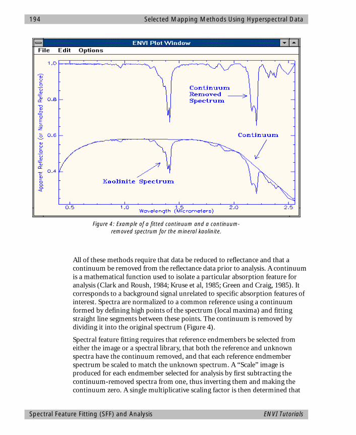
194 Selected Mapping Methods Using Hyperspectral Data
All of these methods require that data be reduced to reflectance and that a continuum be removed from the reflectance data prior to analysis. A continuum is a mathematical function used to isolate a particular absorption feature for analysis (Clark and Roush, 1984; Kruse et al, 1985; Green and Craig, 1985). It corresponds to a background signal unrelated to specific absorption features of interest. Spectra are normalized to a common reference using a continuum formed by defining high points of the spectrum (local maxima) and fitting straight line segments between these points. The continuum is removed by dividing it into the original spectrum (Figure 4).
Spectral feature fitting requires that reference endmembers be selected from either the image or a spectral library, that both the reference and unknown spectra have the continuum removed, and that each reference endmember spectrum be scaled to match the unknown spectrum. A “Scale” image is produced for each endmember selected for analysis by first subtracting the continuum-removed spectra from one, thus inverting them and making the continuum zero. A single multiplicative scaling factor is then determined that
Figure 4: Example of a fitted continuum and a continuum-removed spectrum for the mineral kaolinite.
Spectral Feature Fitting (SFF) and Analysis ENVI Tutorials

Selected Mapping Methods Using Hyperspectral Data 195
makes the reference spectrum match the unknown spectrum. Assuming that a reasonable spectral range has been selected, a large scaling factor is equivalent to a deep spectral feature, while a small scaling factor indicates a weak spectral feature.
.A least-squares-fit is then calculated band-by-band between each reference endmember and the unknown spectrum. The total root-mean-square (RMS) error is used to form an RMS image for each endmember. An optional ratio image of Scale/RMS provides a “Fit” image that is a measure of how well the unknown spectrum matches the reference spectrum on a pixel-by-pixel basis.
Open and Load the Continuum-Removed DataFor the purposes of this exercise, you will not create your own continuum-removed data, they have been pre-calculated.
• If you want to perform this operation on your own:
1. Open the file CUP95EFF.INT and select Spectral Tools->Continuum Removal.
2. Select the CUP95EFF.INT file, perform spectral subsetting if desired to limit the spectral range for continuum removal, and click “OK”.
3. Enter the continuum-removed output file name in the Continuum Removal Parameters dialog and click “OK” to create the continuum-removed image.
This image will have the same number of spectral bands as the input image.
• If not creating your own continuum-removed file:
1. Open the file CUP95_CR.DAT.
This is the continuum-removed data (floating point 0 - 1.0 range) derived from the 1995 AVIRIS Effort-calibrated apparent reflectance as described above.
2. Load band 193 (2.20 µm) as a grayscale image by clicking “Load Band” in the Available Bands List.
3. Start a Z-Profile by clicking the right mouse button in the Main Image display and selecting Functions->Profiles->Z-Profile.
4. Select Options->Auto-scale Y-axis Off in the Spectral Profile window.
5. Choose Edit->Plot Parameters in the Spectral Profile window, click on the “Y-Axis” radio button, and enter the range 0.5 - 1.0 in the appropriate text boxes for the Y-axis.
ENVI Tutorials Spectral Feature Fitting (SFF) and Analysis
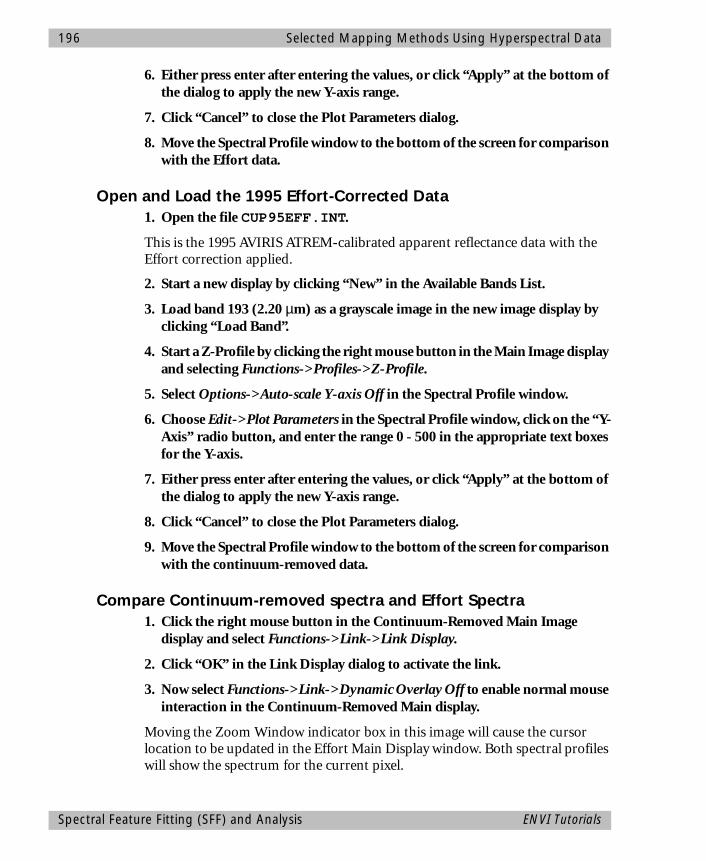
196 Selected Mapping Methods Using Hyperspectral Data
6. Either press enter after entering the values, or click “Apply” at the bottom of the dialog to apply the new Y-axis range.
7. Click “Cancel” to close the Plot Parameters dialog.
8. Move the Spectral Profile window to the bottom of the screen for comparison with the Effort data.
Open and Load the 1995 Effort-Corrected Data1. Open the file CUP95EFF.INT.
This is the 1995 AVIRIS ATREM-calibrated apparent reflectance data with the Effort correction applied.
2. Start a new display by clicking “New” in the Available Bands List.
3. Load band 193 (2.20 µm) as a grayscale image in the new image display by clicking “Load Band”.
4. Start a Z-Profile by clicking the right mouse button in the Main Image display and selecting Functions->Profiles->Z-Profile.
5. Select Options->Auto-scale Y-axis Off in the Spectral Profile window.
6. Choose Edit->Plot Parameters in the Spectral Profile window, click on the “Y-Axis” radio button, and enter the range 0 - 500 in the appropriate text boxes for the Y-axis.
7. Either press enter after entering the values, or click “Apply” at the bottom of the dialog to apply the new Y-axis range.
8. Click “Cancel” to close the Plot Parameters dialog.
9. Move the Spectral Profile window to the bottom of the screen for comparison with the continuum-removed data.
Compare Continuum-removed spectra and Effort Spectra1. Click the right mouse button in the Continuum-Removed Main Image
display and select Functions->Link->Link Display.
2. Click “OK” in the Link Display dialog to activate the link.
3. Now select Functions->Link->Dynamic Overlay Off to enable normal mouse interaction in the Continuum-Removed Main display.
Moving the Zoom Window indicator box in this image will cause the cursor location to be updated in the Effort Main Display window. Both spectral profiles will show the spectrum for the current pixel.
Spectral Feature Fitting (SFF) and Analysis ENVI Tutorials
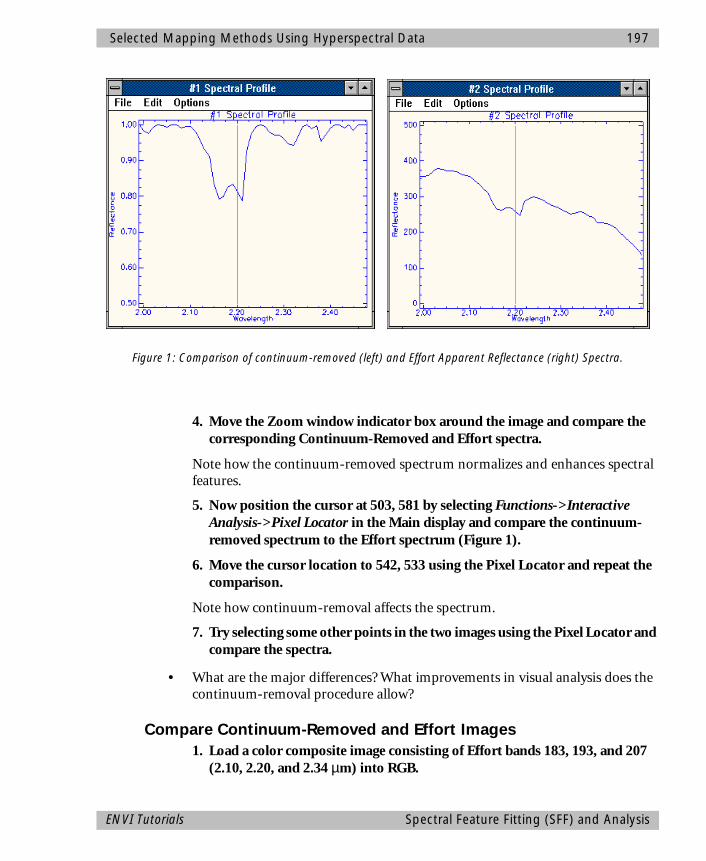
Selected Mapping Methods Using Hyperspectral Data 197
4. Move the Zoom window indicator box around the image and compare the corresponding Continuum-Removed and Effort spectra.
Note how the continuum-removed spectrum normalizes and enhances spectral features.
5. Now position the cursor at 503, 581 by selecting Functions->Interactive Analysis->Pixel Locator in the Main display and compare the continuum-removed spectrum to the Effort spectrum (Figure 1).
6. Move the cursor location to 542, 533 using the Pixel Locator and repeat the comparison.
Note how continuum-removal affects the spectrum.
7. Try selecting some other points in the two images using the Pixel Locator and compare the spectra.
• What are the major differences? What improvements in visual analysis does the continuum-removal procedure allow?
Compare Continuum-Removed and Effort Images1. Load a color composite image consisting of Effort bands 183, 193, and 207
(2.10, 2.20, and 2.34 µm) into RGB.
Figure 1: Comparison of continuum-removed (left) and Effort Apparent Reflectance (right) Spectra.
ENVI Tutorials Spectral Feature Fitting (SFF) and Analysis

198 Selected Mapping Methods Using Hyperspectral Data
2. Click the left mouse button in the Effort Main Image display to activate the dynamic overlay.
3. Compare the continuum-removed image for band 193 (2.20 µm) to the color composite image.
Note the correspondence between dark areas on the continuum-removed image and red-to-purple areas on the color composite. The dark areas are areas with absorption bands near 2.2 µm.
4. Move the Zoom window indicator box to some of these dark areas by dragging with the left mouse button or by clicking in the desired location with the middle mouse button.
5. Compare the corresponding spectral profiles for both the continuum-removed data and the Effort data and note the image colors.
6. Load continuum-removed band 207 (2.34 µm).
Note by moving the Zoom window to the dark areas and examining the spectra that these correspond to absorption features near 2.34 µm in both the continuum-removed and Effort spectra.
Close the Effort Display and Spectral Profile
• Click on one of the Effort bands in the Available Bands List and then click “Close File” at the bottom of the dialog.
The associated display windows and spectral plot will also be closed.
Open and Load the Spectral Feature Fitting Scale and RMS ImagesFor the purposes of this exercise, you will not create your own SFF Scale or RMS data, they have been pre-calculated.
• If you want to perform this operation on your own:
1. Open the file CUP95_CR.DAT and select Spectral Tools->Mapping Methods->Spectral Feature Fitting.
2. Select the CUP95_CR.DAT file, perform spectral subsetting if desired to limit the spectral range for fitting, and click “OK”.
3. Use ENVI’s standardized Endmember Collection dialog to import image or library spectra to use as endmembers in the SFF and click “Apply” in the Endmember Collection dialog.
Spectral Feature Fitting (SFF) and Analysis ENVI Tutorials
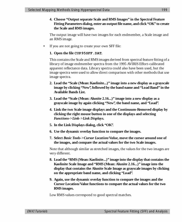
Selected Mapping Methods Using Hyperspectral Data 199
4. Choose “Output separate Scale and RMS Images” in the Spectral Feature Fitting Parameters dialog, enter an output file name, and click “OK” to create the Scale and RMS images.
The output image will have two images for each endmember, a Scale image and an RMS image.
• If you are not going to create your own SFF file:
1. Open the file CUP95SFF.DAT.
This contains the Scale and RMS images derived from spectral feature fitting of a library of image endmember spectra from the 1995 AVIRIS Effort-calibrated apparent reflectance data. Library spectra could also have been used, but the image spectra were used to allow direct comparison with other methods that use image spectra.
2. Load the “Scale (Mean: Kaolinite...)” image into a new display as a grayscale image by clicking “New”, followed by the band name and “Load Band” in the Available Bands List.
3. Load the “Scale (Mean: Alunite 2.16...)” image into a new display as a grayscale image by again clicking “New”, the band name, and “Load”.
4. Link the two Scale image displays and the Continuum-Removed display by clicking the right mouse button in one of the displays and selecting Functions->Link->Link Displays.
5. In the Link Displays dialog, click “OK”.
6. Use the dynamic overlay function to compare the images.
7. Select Basic Tools->Cursor Location/Value, move the cursor around one of the images, and compare the actual values for the two Scale images.
Note that although similar as stretched images, the values for the two images are very different.
8. Load the “RMS (Mean: Kaolinite...)” image into the display that contains the Kaolinite Scale Image and “RMS (Mean: Alunite 2.16...)” image into the display that contains the Alunite Scale Image as grayscale images by clicking on the appropriate band name, and clicking “Load”.
9. Again, use the dynamic overlay function to compare the images and the Cursor Location/Value functions to compare the actual values for the two RMS images.
Low RMS values correspond to good spectral matches.
ENVI Tutorials Spectral Feature Fitting (SFF) and Analysis
200 Selected Mapping Methods Using Hyperspectral Data
2-D Scatterplots of SFF Results1. Start 2-D Scatterplots from the RMS (Mean: Kaolinite...) image by clicking
the right mouse button in the Main Image display and selecting Functions->Interactive Analysis->2-D Scatterplots.
2. Choose the Kaolinite Scale and RMS images for Bands X and Y.
3. Draw a Region of Interest (ROI) on the scatterplot at low RMS values for all ranges of Scale by clicking the left mouse button to draw lines connecting the vertices of a polygon and the right mouse button to close the polygon.
Note the highlighted pixels in the RMS Kaolinite.
4. Select the Options->Change Bands in the Scatterplot Window.
5. Load other combinations of Scale and RMS for the various endmembers.
6. Close the 2-D scatterplot by selecting File->Cancel in the Scatterplot window.
7. Select Basic Tools->Display Controls->Close All Plot Windows.
Spectral Feature Fitting Ratios - “Fit” ImagesFor the purposes of this exercise, you will not create your own SFF Fit Images, they have been pre-calculated.
• If you want to perform this operation on your own:
1. Open the file CUP95_CR.DAT and select Spectral Tools->Mapping Methods->Spectral Feature Fitting.
2. Select the CUP95_CR.DAT file, perform spectral subsetting if (desired) to limit the spectral range for fitting, and click “OK”.
3. Use ENVI’s standardized Endmember Collection dialog to import image or library spectra to use as endmembers in the SFF and click “Apply” in the Endmember Collection dialog.
4. Use the toggle arrows in the Spectral Feature Fitting Parameters dialog to select “Output combined (Scale/RMS) images, enter an output file name, and click “OK” to create the Fit images.
The output image will have one Fit image for each endmember.
• If not creating your own SFF file:
1. Open the file CUP95SFR.DAT.
This contains the images that are the ratio of Scale/RMS for each of the endmembers.
Spectral Feature Fitting (SFF) and Analysis ENVI Tutorials
Selected Mapping Methods Using Hyperspectral Data 201
2. Load the “Fit (Mean: Kaolinite...)” image into the existing display containing the continuum-removed data as a grayscale image by entering the appropriate display number in the “Active Display” text box in the Available Bands List.
3. Click on the band name and click “Load Band”.
The bright pixels represent the best fit to the reference endmember spectrum of Kaolinite.
4. Load the “Scale (Mean: Kaolinite...)” and “RMS (Mean: Kaolinite...)” images into the other two displays if not already loaded.
5. Link the image displays and compare the Fit, Scale, and RMS images.
Note how the Scale and RMS image interact to produce the Fit result.
6. Load the Effort data again and extract spectral profiles for the bright pixels in the Fit image.
7. Compare the Fit, Scale, and RMS images as well as the spectral profiles for the other endmembers.
8. Make one or more color composite images by loading Fit images for different endmembers as RGB.
• What conclusions can you draw regarding the effectiveness of spectral feature fitting for identifying specific endmembers?
Close Files and Exit ENVI.
• When you have finished your ENVI session, click “Quit” or “Exit” on the ENVI Main Menu, then type exit at the IDL command prompt.
If you are using ENVI RT, quitting ENVI will take you back to your operating system.
ReferencesClark, R. N., and Roush, T. L., 1984, Reflectance spectroscopy: Quantitative analysis techniques for remote sensing applications: Journal of Geophysical Research, v. 89, no. B7, pp. 6329-6340.
Clark, R. N., King, T. V. V., and Gorelick, N. S., 1987, Automatic continuum analysis of reflectance spectra: in Proceedings, Third AIS workshop, 2-4 June, 1987, JPL Publication 87-30, Jet Propulsion Laboratory, Pasadena, California, p. 138-142.
ENVI Tutorials References
202 Selected Mapping Methods Using Hyperspectral Data
Clark, R. N., Swayze, G. A., Gallagher, A., King, T. V. V., and Calvin, W. M., 1993, The U. S. Geological Survey Digital Spectral Library: Version 1: 0.2 to 3.0 mm: U. S. Geological Survey, Open File Report 93-592, 1340 p.
Clark, R. N., Gallagher, A. J., and Swayze, G. A., 1990, Material absorption band depth mapping of imaging spectrometer data using the complete band shape least-squares algorithm simultaneously fit to multiple spectral features from multiple materials: in Proceedings of the Third Airborne Visible/Infrared Imaging Spectrometer (AVIRIS) Workshop, JPL Publication 90-54, p. 176 - 186.
Clark, R. N., Swayze, G. A., Gallagher, A., Gorelick, N., and Kruse, F. A., 1991, Mapping with imaging spectrometer data using the complete band shape least-squares algorithm simultaneously fit to multiple spectral features from multiple materials: in Proceedings, 3rd Airborne Visible/Infrared Imaging Spectrometer (AVIRIS) workshop, JPL Publication 91-28, p. 2-3.
Clark, R. N., Swayze, G. A., and Gallagher, A., 1992, Mapping the mineralogy and lithology of Canyonlands, Utah with imaging spectrometer data and the multiple spectral feature mapping algorithm: in Summaries of the Third Annual JPL Airborne Geoscience Workshop, JPL Publication 92-14, v 1, p. 11-13.
Center for the Study of Earth from Space (CSES), 1992, SIPS User’s Guide, The Spectral Image Processing System, v. 1.1, University of Colorado, Boulder,74 p.
Crowley, J. K., and Clark, R. N., 1992, AVIRIS study of Death Valley evaporite deposits using least-squares band-fitting methods: in Summaries of the Third Annual JPL Airborne Geoscience Workshop, JPL Publication 92-14, v 1, p. 29-31.
Clark, R. N., and Swayze, G. A., 1995, Mapping minerals, amorphous materials, environmental materials, vegetation, water, ice, and snow, and other materials: The USGS Tricorder Algorithm: in Summaries of the Fifth Annual JPL Airborne Earth Science Workshop, JPL Publication 95-1, p. 39 - 40.
Green, A. A., and Craig, M. D., 1985, Analysis of aircraft spectrometer data with logarithmic residuals: in Proceedings, AIS workshop, 8-10 April, 1985, JPL Publication 85-41, Jet Propulsion Laboratory, Pasadena, California, p. 111-119.
Kruse, F. A., Raines, G. L., and Watson, K., 1985, Analytical techniques for extracting geologic information from multichannel airborne spectroradiometer and airborne imaging spectrometer data: in Proceedings, International Symposium on Remote Sensing of Environment, Thematic Conference on Remote Sensing for Exploration Geology, 4th, Environmental Research Institute of Michigan, Ann Arbor, p. 309-324.
Kruse, F. A., Calvin, W. M., and Seznec, O., 1988, Automated extraction of absorption features from Airborne Visible/Infrared Imaging Spectrometer (AVIRIS) and Geophysical Environmental Research imaging spectrometer (GERIS) data: In Proceedings of the Airborne Visible/Infrared Imaging
References ENVI Tutorials

Selected Mapping Methods Using Hyperspectral Data 203
Spectrometer (AVIRIS) performance evaluation workshop, JPL Publication 88-38, p. 62-75.
Kruse, F. A., 1988, Use of Airborne Imaging Spectrometer data to map minerals associated with hydrothermally altered rocks in the northern Grapevine Mountains, Nevada and California: Remote Sensing of Environment, v. 24, no. 1, pp. 31-51.
Kruse, F. A., 1990, Artificial Intelligence for Analysis of Imaging Spectrometer Data: Proceedings, ISPRS Commission VII, Working Group 2: "Analysis of High Spectral Resolution Imaging Data", Victoria, B. C., Canada, 17-21 September, 1990, p. 59-68.
Kruse, F. A., Lefkoff, A. B., Boardman, J. W., Heidebrecht, K. B., Shapiro, A. T., Barloon, J. P., and Goetz, A. F. H., 1993a, The spectral image processing system (SIPS) - Interactive visualization and analysis of imaging spectrometer data: Remote Sensing of Environment, v. 44, p. 145 - 163.
Kruse, F. A., and Lefkoff, A. B., 1993b, Knowledge-based geologic mapping with imaging spectrometers: Remote Sensing Reviews, Special Issue on NASA Innovative Research Program (IRP) results, v. 8, p. 3 - 28.
Kruse, F. A., Lefkoff, A. B., and Dietz, J. B., 1993c, Expert System-Based Mineral Mapping in northern Death Valley, California/Nevada using the Airborne Visible/Infrared Imaging Spectrometer (AVIRIS): Remote Sensing of Environment, Special issue on AVIRIS, May-June 1993, v. 44, p. 309 - 336.
Swayze, g. A., and Clark, R. N., 1995, Spectral identification of minerals using imaging spectrometry data: evaluating the effects of signal to noise and spectral resolution using the Tricorder Algorithm: in Summaries of the Fifth Annual JPL airborne Earth Science Workshop, JPL Publication 95-1, p. 157 - 158.
Yamaguchi, Yasushi, and Lyon, R. J. P., 1986, Identification of clay minerals by feature coding of near-infrared spectra: in Proceedings, International Symposium on Remote Sensing of Environment, Fifth Thematic Conference, "Remote Sensing for Exploration Geology", Reno, Nevada, 29 September- 2 October, 1986, Environmental Research Institute of Michigan, Ann Arbor, p. 627-636.
ENVI Tutorials References

204 Selected Mapping Methods Using Hyperspectral Data
References ENVI Tutorials
ENVI Tutorial #10
Advanced Hyperspectral Analysis
The following topics are covered in this tutorial:
Overview of This Tutorial ......................................................................................206MNF Transform Data, Endmembers, and Spectral Unmixing.................................207Pixel Purity Index ..................................................................................................211n-Dimensional Visualization ..................................................................................214Matched Filter Background ...................................................................................219Matched Filter Results ...........................................................................................219Background: Unmixing. ........................................................................................220Unmixing Results ..................................................................................................224References ............................................................................................................226
205
206 Advanced Hyperspectral Analysis
Overview of This TutorialThis tutorial is designed to introduce you to advanced concepts and procedures for analysis of imaging spectrometer data or hyperspectral images. We will use 1995 Airborne Visible/Infrared Imaging Spectrometer (AVIRIS) data from Cuprite, Nevada, to investigate sub-pixel properties of hyperspectral data and advanced techniques for identification and quantification of mineralogy. We will use “Effort” “polished” ATREM-calibrated data, and review matched filter and spectral unmixing results. This tutorial is designed to be completed in two to four hours.
Files Used in This TutorialYou must have the ENVI TUTORIALS & DATACD-ROM mounted on your system to access thefiles used by this tutorial, or copy the files to yourdisk.
The files used in this tutorial are contained in the C95AVSUB subdirectory of the ENVIDATA directory on the ENVI TUTORIALS & DATA CD-ROM.
The files listed below, along with their associated .hdr files, are required to run this exercise. Optional spectral library files listed below may also be used if more detailed comparisons are desired. Selected data files have been converted to integer format by multiplying the reflectance values by 1000 because of disk space considerations. Values of 1000 in the files represent reflectance values of 1.0.
Required FilesCUP95EFF.INT “Effort” corrected
ATREM apparent reflec-tance data, 56 bands, 1.96 - 2.51 mm.
CUP95MNF.DAT First 25 MNF bands.
CUP95MNF.ASC MNF eigenvalue spectrum
CUP95PPI.DAT Pixel Purity Index (PPI) Image
Topics Covered in This Tutorial
MNF Transform and Determination of Spectral Endmembers• Background Minimum Noise
Fraction (MNF)• Open and Load MNF Images• Review MNF Eigenvalue Plot• Compare MNF Images• Examine MNF Scatterplots• Use Scatterplots to Select
Endmembers• Compare ROIs to Previously Saved
ROIs
Pixel Purity Index• Display and Analyze the Pixel
Purity Index• Threshold PPI to Regions of
Interest
n-Dimensional Visualization• Compare n-D Visualization with 2-
D Scatterplots• Restore n-D Visualizer State• Use the n-D Visualizer• Paint Endmembers• Export Your Own ROIs• Plot Endmember Spectra
Background: Matched Filtering• Maximizing the response of a
known endmember in the presence of a composite unknown background
Matched Filter Results• Open and Display the Matched
Filter Results• Set Thresholds to identify best
matches
Endmembers, and Spectral Mixing
Overview of This Tutorial ENVI Tutorials
Advanced Hyperspectral Analysis 207
CUP95PPI.ROI Region of Interest for PPI values greater than 1750
CUP95PPI.NDV N-D Visualizer Saved State File.
CUP95NDV.ROI ASCII file spectral endmembers corresponding to the N-D Visualizer Saved State File
CUP95_EM.ASC ASCII file of 11 spectral endmembers elected using the PPI threshold, MNF images, and n-D Visualization - used in Matched Filtering and Unmixing
CUP95MAT.DAT Match Filter Results—Mineral Images
CUP95UNM.DAT Unmixing Results—Fractional Abundance imag-es.
Optional FilesJPL1.SLI JPL Spectral Library in ENVI format.
USGS_MIN.SLI USGS Spectral Library in ENVI format.
Open and Load the 1995 Effort-Corrected Data1. Open the file CUP95EFF.INT.
This is the 1995 AVIRIS ATREM-calibrated apparent reflectance data with the Effort correction applied.
2. Start a new display by clicking on the “New” button in the Available Bands List.
3. Load band 193 as a grayscale image in the new image display by clicking on the “Load Band” button.
These data will be used for comparison with MNF bands and to extract spectral endmembers for PPI results.
MNF Transform Data, Endmembers, and Spectral Unmixing
Background: Minimum Noise FractionThe minimum noise fraction (MNF) transformation is used to determine the inherent dimensionality of image data, to segregate noise in the data, and to reduce the computational requirements for subsequent processing (See Boardman and Kruse, 1994). The MNF transform as modified from Green et al. (1988) and implemented in ENVI is essentially two cascaded Principal Components transformations. The first transformation, based on an estimated noise covariance matrix, decorrelates and rescales the noise in the data. This first
ENVI Tutorials MNF Transform Data, Endmembers, and Spectral Unmixing
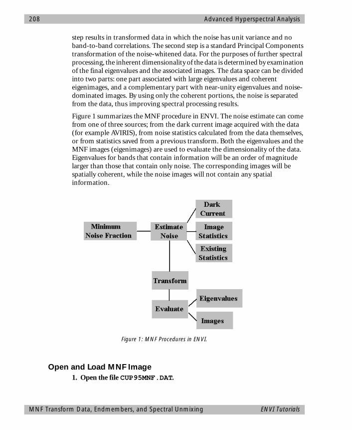
208 Advanced Hyperspectral Analysis
step results in transformed data in which the noise has unit variance and no band-to-band correlations. The second step is a standard Principal Components transformation of the noise-whitened data. For the purposes of further spectral processing, the inherent dimensionality of the data is determined by examination of the final eigenvalues and the associated images. The data space can be divided into two parts: one part associated with large eigenvalues and coherent eigenimages, and a complementary part with near-unity eigenvalues and noise-dominated images. By using only the coherent portions, the noise is separated from the data, thus improving spectral processing results.
Figure 1 summarizes the MNF procedure in ENVI. The noise estimate can come from one of three sources; from the dark current image acquired with the data (for example AVIRIS), from noise statistics calculated from the data themselves, or from statistics saved from a previous transform. Both the eigenvalues and the MNF images (eigenimages) are used to evaluate the dimensionality of the data. Eigenvalues for bands that contain information will be an order of magnitude larger than those that contain only noise. The corresponding images will be spatially coherent, while the noise images will not contain any spatial information.
Open and Load MNF Image1. Open the file CUP95MNF.DAT.
Figure 1: MNF Procedures in ENVI.
MNF Transform Data, Endmembers, and Spectral Unmixing ENVI Tutorials
Advanced Hyperspectral Analysis 209
This dataset contains the first 25 MNF bands (floating point) from the 1995 Cuprite Effort data.
2. Load the first MNF band as a grayscale image in a new image display by clicking on the band name, clicking “New”, and then “Load Band” in the Available Bands List.
Compare MNF Images1. Load several other MNF bands, either one at a time for individual
examination or in RGB composites for intercomparison.
2. Use the Z-Profile, image linking, and Dynamic Overlay tools to compare MNF-spectra with Apparent Reflectance spectra from the Effort image.
3. Try to determine the relation(s) between the MNF image and the apparent reflectance images. Relate MNF band number to MNF image quality.
Examine MNF Scatterplots 1. Use 2-D scatter plots in forward and inverse mapping modes to understand
the MNF images.
2. Be sure to examine the high variance (low band number) MNF bands. Also be sure to examine at least one scatterplot of a low variance (high band number) MNF band (change the bands by selecting Options->Change Bands in the Scatter Plot window).
Note the “corners” on some MNF scatterplots (Figure 2).
3. Use linked windows, overlays, and Z-profiles to understand the reflectance spectra of the MNF corner pixels.
Note when the MNF data stops being “pointy” and begins being “fuzzy” and the relation between scatterplot pixel location and spectral mixing as determined from image color and individual reflectance spectra.
• How do you explain these patterns? How can you exploit them?
Use Scatterplots to Select EndmembersWe will now investigate the possibilities of deriving unmixing endmembers from the data using MNF images and the 2-D scatterplot tools.
1. Load a scatterplot of MNF bands 1 and 2.
2. In the scatter plot, use the ROI drawing functions to circle the extreme few pixels in one or more of the corners or arms of the data cloud.
ENVI Tutorials MNF Transform Data, Endmembers, and Spectral Unmixing
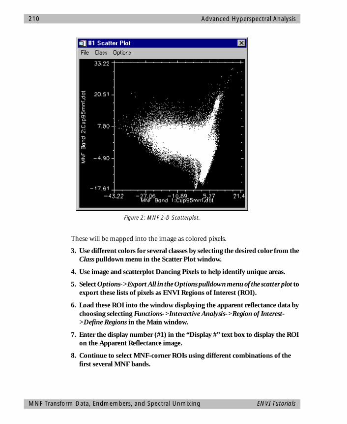
210 Advanced Hyperspectral Analysis
These will be mapped into the image as colored pixels.
3. Use different colors for several classes by selecting the desired color from the Class pulldown menu in the Scatter Plot window.
4. Use image and scatterplot Dancing Pixels to help identify unique areas.
5. Select Options->Export All in the Options pulldown menu of the scatter plot to export these lists of pixels as ENVI Regions of Interest (ROI).
6. Load these ROI into the window displaying the apparent reflectance data by choosing selecting Functions->Interactive Analysis->Region of Interest->Define Regions in the Main window.
7. Enter the display number (#1) in the “Display #” text box to display the ROI on the Apparent Reflectance image.
8. Continue to select MNF-corner ROIs using different combinations of the first several MNF bands.
Figure 2: MNF 2-D Scatterplot.
MNF Transform Data, Endmembers, and Spectral Unmixing ENVI Tutorials
Advanced Hyperspectral Analysis 211
9. Use the “Mean All” button to extract the mean apparent reflectance spectra of the ROIs.
10. Do the same for the MNF data by entering the display number (#2) in the Display # text box and extracting the mean MNF spectra.
11. Use the linked windows and Z-profiles to examine the relations between the MNF and reflectance spectra.
Note that corner pixels on the scatterplots generally make good endmember estimates. However, note also the occurrence of overlapping or repeat ROIs. This is a limitation of examining the data in a pairwise fashion (2-D).
12. Close the 2-D scatterplot by selecting File->Cancel in the Scatter Plot window.
Pixel Purity IndexIn this portion of the exercise, you will examine the role of convex geometry in determining the relative purity of pixels. Separating purer from more mixed pixels reduces the number of pixels to be analyzed for endmember determination and makes separation and identification of endmembers easier.
The “Pixel-Purity-Index” (PPI) is a means of finding the most “spectrally pure,” or extreme, pixels in multispectral and hyperspectral images. See Boardman et al. (1995). The most spectrally pure pixels typically correspond to mixing endmembers. The Pixel Purity Index is computed by repeatedly projecting n-dimensional scatter plots onto a random unit vector. The extreme pixels in each projection are recorded and the total number of times each pixel is marked as extreme is noted. A Pixel Purity Index (PPI) image is created in which the DN of each pixel corresponds to the number of times that pixel was recorded as extreme. Figure 3 summarizes the use of PPI in ENVI.
Display and Analyze the Pixel Purity Index1. Open the file CUP95PPI.DAT and display it as a grayscale image.
Brighter pixels represent more spectrally extreme “hits” and indicate pixels that are more spectrally pure. Darker pixels are less spectrally pure.
1. Try various interactive stretches from the Contrast Stretch pulldown menu under the ENVI File menu to understand the PPI image’s histogram and data distribution.
• Why is the histogram skewed to the low values. What does this mean from a mixing point of view?
ENVI Tutorials Pixel Purity Index
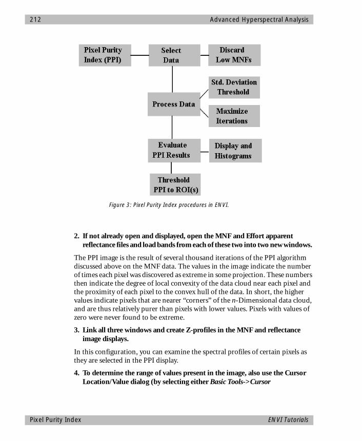
212 Advanced Hyperspectral Analysis
2. If not already open and displayed, open the MNF and Effort apparent reflectance files and load bands from each of these two into two new windows.
The PPI image is the result of several thousand iterations of the PPI algorithm discussed above on the MNF data. The values in the image indicate the number of times each pixel was discovered as extreme in some projection. These numbers then indicate the degree of local convexity of the data cloud near each pixel and the proximity of each pixel to the convex hull of the data. In short, the higher values indicate pixels that are nearer “corners” of the n-Dimensional data cloud, and are thus relatively purer than pixels with lower values. Pixels with values of zero were never found to be extreme.
3. Link all three windows and create Z-profiles in the MNF and reflectance image displays.
In this configuration, you can examine the spectral profiles of certain pixels as they are selected in the PPI display.
4. To determine the range of values present in the image, also use the Cursor Location/Value dialog (by selecting either Basic Tools->Cursor
Figure 3: Pixel Purity Index procedures in ENVI.
Pixel Purity Index ENVI Tutorials

Advanced Hyperspectral Analysis 213
Location/Value on the ENVI Main menu or Functions->Interactive Analysis Cursor Location/Value in the Main window).
5. Move around the image using the Z-profiles and dynamic overlay tools to examine the purest pixels both spatially and spectrally.
• Do any of the high PPI values fall in the regions of the image corresponding to the 2-D scatterplot corners you picked in the previous exercise? Why?
Threshold PPI to Regions of Interest1. Restore the file CUP95PPI.ROI using the “Restore ROI” button in the Region
of Interest Controls dialog.
This is a list of pixels where the PPI value is over 1000.
• How many high PPI pixels are there?
Now try making some of your own thresholded PPI Regions of Interest.
2. Select Functions->Display Enhancements->Interactive Stretching in the PPI image.
3. Determine a threshold to use for choosing only the purest pixels by using the left mouse button to read values off the histogram.
4. Click the middle mouse button in the histogram to zoom in on the lower end of the distribution.
5. Select a value on the high tail of the histogram as the minimum threshold (if you have difficulty with this try a value of “2000” as a starting point).
6. Select Functions->Region of Interest->Image Threshold to ROI in the Main window to create an ROI containing only the pixels with high PPI values.
7. Choose the PPI file for thresholding and enter the value selected above for the minimum threshold and click “OK”.
ENVI will determine the number of pixels that meet the selected criteria and post a message.
• For the purposes of this exercise, if your threshold results in more than 2000 pixels being selected, you should select a higher minimum threshold.
8. Click “OK” and a standard ENVI ROI will be created and listed in the Region of Interest Controls dialog.
Only those pixels with values greater than the selected minimum will be included in the ROI built from the PPI image.
ENVI Tutorials Pixel Purity Index
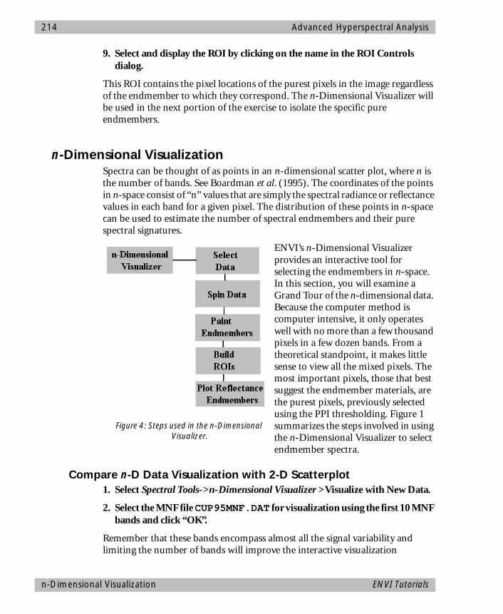
214 Advanced Hyperspectral Analysis
9. Select and display the ROI by clicking on the name in the ROI Controls dialog.
This ROI contains the pixel locations of the purest pixels in the image regardless of the endmember to which they correspond. The n-Dimensional Visualizer will be used in the next portion of the exercise to isolate the specific pure endmembers.
n-Dimensional VisualizationSpectra can be thought of as points in an n-dimensional scatter plot, where n is the number of bands. See Boardman et al. (1995). The coordinates of the points in n-space consist of “n” values that are simply the spectral radiance or reflectance values in each band for a given pixel. The distribution of these points in n-space can be used to estimate the number of spectral endmembers and their pure spectral signatures.
ENVI’s n-Dimensional Visualizer provides an interactive tool for selecting the endmembers in n-space. In this section, you will examine a Grand Tour of the n-dimensional data. Because the computer method is computer intensive, it only operates well with no more than a few thousand pixels in a few dozen bands. From a theoretical standpoint, it makes little sense to view all the mixed pixels. The most important pixels, those that best suggest the endmember materials, are the purest pixels, previously selected using the PPI thresholding. Figure 1 summarizes the steps involved in using the n-Dimensional Visualizer to select endmember spectra.
Compare n-D Data Visualization with 2-D Scatterplot1. Select Spectral Tools->n-Dimensional Visualizer >Visualize with New Data.
2. Select the MNF file CUP95MNF.DAT for visualization using the first 10 MNF bands and click “OK”.
Remember that these bands encompass almost all the signal variability and limiting the number of bands will improve the interactive visualization
Figure 4: Steps used in the n-Dimensional Visualizer.
n-Dimensional Visualization ENVI Tutorials
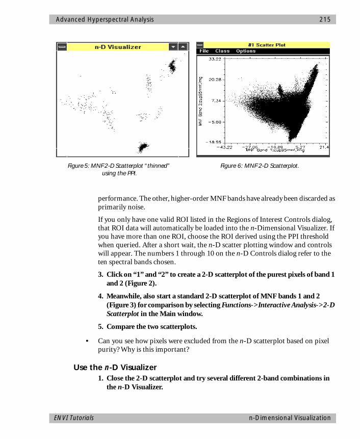
Advanced Hyperspectral Analysis 215
performance. The other, higher-order MNF bands have already been discarded as primarily noise.
If you only have one valid ROI listed in the Regions of Interest Controls dialog, that ROI data will automatically be loaded into the n-Dimensional Visualizer. If you have more than one ROI, choose the ROI derived using the PPI threshold when queried. After a short wait, the n-D scatter plotting window and controls will appear. The numbers 1 through 10 on the n-D Controls dialog refer to the ten spectral bands chosen.
3. Click on “1” and “2” to create a 2-D scatterplot of the purest pixels of band 1 and 2 (Figure 2).
4. Meanwhile, also start a standard 2-D scatterplot of MNF bands 1 and 2 (Figure 3) for comparison by selecting Functions->Interactive Analysis->2-D Scatterplot in the Main window.
5. Compare the two scatterplots.
• Can you see how pixels were excluded from the n-D scatterplot based on pixel purity? Why is this important?
Use the n-D Visualizer1. Close the 2-D scatterplot and try several different 2-band combinations in
the n-D Visualizer.
Figure 5: MNF 2-D Scatterplot “thinned” using the PPI.
Figure 6: MNF 2-D Scatterplot.
EN
VI Tutorials n-Dimensional Visualization
216 Advanced Hyperspectral Analysis
Note the shape of the data clouds. Be sure to examine some of the higher order MNF bands.
2. Now try several three-band combinations by clicking on three of the band numbers.
3. When only 3 bands are selected, you can “drive” the view of the projection by clicking on the arrow toggle button near the bottom of the n-D Controls dialog to toggle the “Drive Axes” option.
4. Subsequently clicking and dragging with the left mouse button in the n-D Visualizer rotates the projection.
Again, note the shape of the data clouds. Be sure to examine some of the higher order MNF bands.
5. Toggle back to “Define ROI” when finished with the 3-D visualization; we will use the ROIs in higher dimensional rotations.
6. Click on the “Start” button to start the “Grand Tour.”
This is an animation of random projections of n-Dimensional space into the scatter plot. In this mode, any number of bands can be examined simultaneously.
7. Click on bands 1, 2, 3, 4, and 5 to view a projection of 5-D data.
8. Click on bands again to deselect them.
9. Try a few different combinations of 2, 3, and more different bands to get a feeling for the n-D data.
10. Try 9 versus 10 to see how it compares to 1 versus 2.
11. While the data are rotating, you can stop and start the rotation by clicking “Start/Stop”.
12. Click “Axes” to display the axes for the various bands in the n-Dimensional projection.
Note how the rotations seem different when more than three bands are included. This is the result of dimensions greater than 3 being “folded” in upon themselves in the projection. This should convince you that the data is truly high dimensional and why 2-D scatterplots are inadequate for dealing with hyperspectral data.
Restore n-D Visualizer Saved State1. Start another n-D Visualizer session using previously saved parameters and
“Painted” endmembers by selecting Spectral Tools->n-D Visualizer->Visualize with Previously Saved Data.
n-Dimensional Visualization ENVI Tutorials

Advanced Hyperspectral Analysis 217
1. Select the file CUP95PPI.NDV.
2. Click on the Start/Stop button to start rotating the data.
The colored pixels in the visualizer represent previously selected endmembers.
3. Examine different projections and numbers of bands in the visualizer.
4. Click on “Start/Stop” to stop the rotation.
5. Click “Delete All” in the Region of Interest Controls dialog to remove all previous regions of interest.
6. Now select Options->Export All in the n-D Visualizer Controls dialog.
1. In the Region of Interest Controls dialog, make sure that the display is set to the Effort apparent reflectance image and then click “Mean All” to extract average reflectance spectra for all of the endmembers.
2. Examine the relations between reflectance spectra and the painted pixels in the n-D Visualizer.
Pay particular attention to similar spectra and the positions of painted clusters.
Paint Your Own Endmembers1. Go back to your original n-Dimensional Visualizer Controls and restart the
rotation using the “Start/Stop” button.
2. When you see an interesting projection (one with points or corners), stop the rotation, select a color from the list under the Class pulldown menu, and use the cursor to circle the points at one or more of the corners.
3. Use the left mouse button to define the segments of a ROI in the scatterplot, and the right mouse button to complete the ROI.
4. Continue spinning the data and update classes as needed as they split up in further projections.
Link the n-D Visualizer to Spectral ProfilesYou can view reflectance spectra for specific endmembers while you’re painting endmember and rotating the scatterplot. This allows you to preview spectra before finalizing spectral classes
1. Select Options->Z-Profile in the n-D Controls dialog. Choose the reflectance data CUP95EFF.INT from the list and click OK. A blank spectral plot appears.
ENVI Tutorials n-Dimensional Visualization
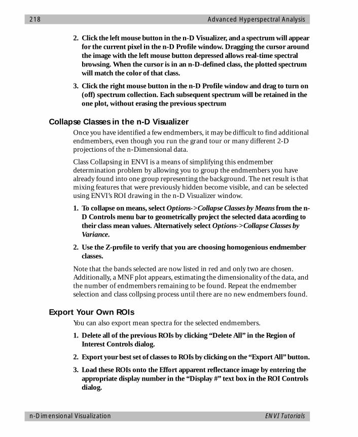
218 Advanced Hyperspectral Analysis
2. Click the left mouse button in the n-D Visualizer, and a spectrum will appear for the current pixel in the n-D Profile window. Dragging the cursor around the image with the left mouse button depressed allows real-time spectral browsing. When the cursor is in an n-D-defined class, the plotted spectrum will match the color of that class.
3. Click the right mouse button in the n-D Profile window and drag to turn on (off) spectrum collection. Each subsequent spectrum will be retained in the one plot, without erasing the previous spectrum
Collapse Classes in the n-D VisualizerOnce you have identified a few endmembers, it may be difficult to find additional endmembers, even though you run the grand tour or many different 2-D projections of the n-Dimensional data.
Class Collapsing in ENVI is a means of simplifying this endmember determination problem by allowing you to group the endmembers you have already found into one group representing the background. The net result is that mixing features that were previously hidden become visible, and can be selected using ENVI’s ROI drawing in the n-D Visualizer window.
1. To collapse on means, select Options->Collapse Classes by Means from the n-D Controls menu bar to geometrically project the selected data acording to their class mean values. Alternatively select Options->Collapse Classes by Variance.
2. Use the Z-profile to verify that you are choosing homogenious endmember classes.
Note that the bands selected are now listed in red and only two are chosen. Additionally, a MNF plot appears, estimating the dimensionality of the data, and the number of endmembers remaining to be found. Repeat the endmember selection and class collpsing process until there are no new endmembers found.
Export Your Own ROIsYou can also export mean spectra for the selected endmembers.
1. Delete all of the previous ROIs by clicking “Delete All” in the Region of Interest Controls dialog.
2. Export your best set of classes to ROIs by clicking on the “Export All” button.
3. Load these ROIs onto the Effort apparent reflectance image by entering the appropriate display number in the “Display #” text box in the ROI Controls dialog.
n-Dimensional Visualization ENVI Tutorials
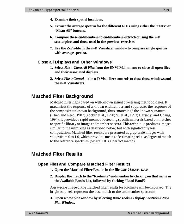
Advanced Hyperspectral Analysis 219
4. Examine their spatial locations.
5. Extract the average spectra for the different ROIs using either the “Stats” or “Mean All” buttons.
6. Compare these endmembers to endmembers extracted using the 2-D scatterplots and those used in the previous exercises.
7. Use the Z-Profile in the n-D Visualizer window to compare single spectra with average spectra.
Close all Displays and Other Windows1. Select File->Close All Files from the ENVI Main menu to close all open files
and their associated displays.
2. Select File->Cancel in the n-D Visualizer controls to close those windows and the n-D Visualizers.
Matched Filter BackgroundMatched filtering is based on well-known signal processing methodologies. It maximizes the response of a known endmember and suppresses the response of the composite unknown background, thus “matching” the known signature (Chen and Reed, 1987; Stocker et al., 1990; Yu et al., 1993; Harsanyi and Chang, 1994). It provides a rapid means of detecting specific minerals based on matches to specific library or image endmember spectra. This technique produces images similar to the unmixing as described below, but with significantly less computation. Matched filter results are presented as gray-scale images with values from 0 to 1.0, which provide a means of estimating relative degree of match to the reference spectrum (where 1.0 is a perfect match).
Matched Filter Results
Open Files and Compare Matched Filter Results1. Open the Matched Filter Results in the file CUP95MAT.DAT.
2. Display the match to the “Kaolinite” endmember by clicking on that name in the Available Bands List, followed by clicking “Load Band”.
A grayscale image of the matched filter results for Kaolinite will be displayed. The brightest pixels represent the best match to the endmember spectrum.
3. Open a new plot window by selecting Basic Tools->Display Controls->New Plot Window.
ENVI Tutorials Matched Filter Background
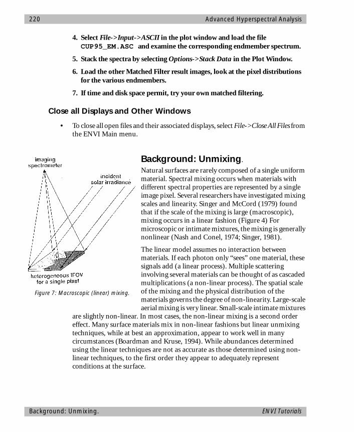
220 Advanced Hyperspectral Analysis
Background: Unmixing. ENVI Tutorials
4. Select File->Input->ASCII in the plot window and load the file CUP95_EM.ASC and examine the corresponding endmember spectrum.
5. Stack the spectra by selecting Options->Stack Data in the Plot Window.
6. Load the other Matched Filter result images, look at the pixel distributions for the various endmembers.
7. If time and disk space permit, try your own matched filtering.
Close all Displays and Other Windows
• To close all open files and their associated displays, select File->Close All Files from the ENVI Main menu.
Background: Unmixing.
Natural surfaces are rarely composed of a single uniform material. Spectral mixing occurs when materials with different spectral properties are represented by a single image pixel. Several researchers have investigated mixing scales and linearity. Singer and McCord (1979) found that if the scale of the mixing is large (macroscopic), mixing occurs in a linear fashion (Figure 4) For microscopic or intimate mixtures, the mixing is generally nonlinear (Nash and Conel, 1974; Singer, 1981).
The linear model assumes no interaction between materials. If each photon only “sees” one material, these signals add (a linear process). Multiple scattering involving several materials can be thought of as cascaded multiplications (a non-linear process). The spatial scale of the mixing and the physical distribution of the materials governs the degree of non-linearity. Large-scale aerial mixing is very linear. Small-scale intimate mixtures
are slightly non-linear. In most cases, the non-linear mixing is a second order effect. Many surface materials mix in non-linear fashions but linear unmixing techniques, while at best an approximation, appear to work well in many circumstances (Boardman and Kruse, 1994). While abundances determined using the linear techniques are not as accurate as those determined using non-linear techniques, to the first order they appear to adequately represent conditions at the surface.
Figure 7: Macroscopic (linear) mixing.
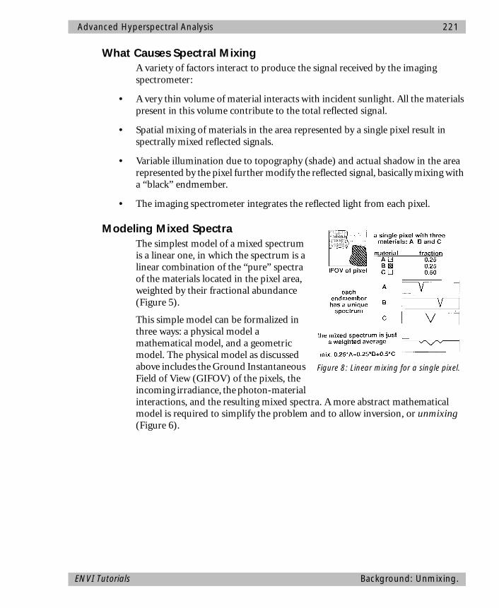
Advanced Hyperspectral Analysis 221
What Causes Spectral Mixing A variety of factors interact to produce the signal received by the imaging spectrometer:
• A very thin volume of material interacts with incident sunlight. All the materials present in this volume contribute to the total reflected signal.
• Spatial mixing of materials in the area represented by a single pixel result in spectrally mixed reflected signals.
• Variable illumination due to topography (shade) and actual shadow in the area represented by the pixel further modify the reflected signal, basically mixing with a “black” endmember.
• The imaging spectrometer integrates the reflected light from each pixel.
Modeling Mixed Spectra The simplest model of a mixed spectrum is a linear one, in which the spectrum is a linear combination of the “pure” spectra of the materials located in the pixel area, weighted by their fractional abundance (Figure 5).
This simple model can be formalized in three ways: a physical model a mathematical model, and a geometric model. The physical model as discussed above includes the Ground Instantaneous Field of View (GIFOV) of the pixels, the incoming irradiance, the photon-material interactions, and the resulting mixed spectra. A more abstract mathematical model is required to simplify the problem and to allow inversion, or unmixing (Figure 6).
Figure 8: Linear mixing for a single pixel.
ENVI Tutorials Background: Unmixing.
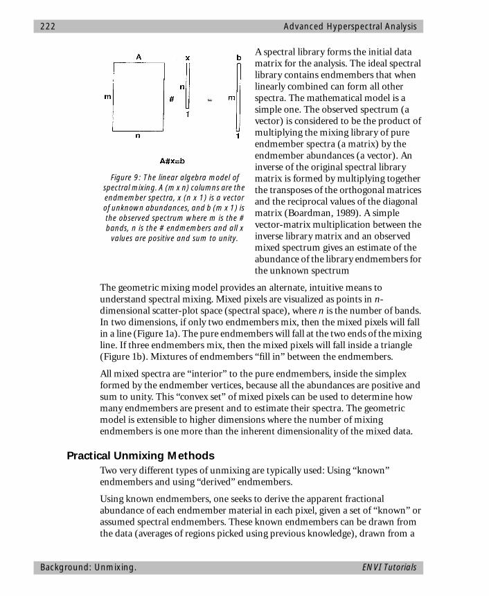
222 Advanced Hyperspectral Analysis
A spectral library forms the initial data matrix for the analysis. The ideal spectral library contains endmembers that when linearly combined can form all other spectra. The mathematical model is a simple one. The observed spectrum (a vector) is considered to be the product of multiplying the mixing library of pure endmember spectra (a matrix) by the endmember abundances (a vector). An inverse of the original spectral library matrix is formed by multiplying together the transposes of the orthogonal matrices and the reciprocal values of the diagonal matrix (Boardman, 1989). A simple vector-matrix multiplication between the inverse library matrix and an observed mixed spectrum gives an estimate of the abundance of the library endmembers for the unknown spectrum
The geometric mixing model provides an alternate, intuitive means to understand spectral mixing. Mixed pixels are visualized as points in n-dimensional scatter-plot space (spectral space), where n is the number of bands. In two dimensions, if only two endmembers mix, then the mixed pixels will fall in a line (Figure 1a). The pure endmembers will fall at the two ends of the mixing line. If three endmembers mix, then the mixed pixels will fall inside a triangle (Figure 1b). Mixtures of endmembers “fill in” between the endmembers.
All mixed spectra are “interior” to the pure endmembers, inside the simplex formed by the endmember vertices, because all the abundances are positive and sum to unity. This “convex set” of mixed pixels can be used to determine how many endmembers are present and to estimate their spectra. The geometric model is extensible to higher dimensions where the number of mixing endmembers is one more than the inherent dimensionality of the mixed data.
Practical Unmixing Methods Two very different types of unmixing are typically used: Using “known” endmembers and using “derived” endmembers.
Using known endmembers, one seeks to derive the apparent fractional abundance of each endmember material in each pixel, given a set of “known” or assumed spectral endmembers. These known endmembers can be drawn from the data (averages of regions picked using previous knowledge), drawn from a
Figure 9: The linear algebra model of spectral mixing. A (m x n) columns are the endmember spectra, x (n x 1) is a vector of unknown abundances, and b (m x 1) is the observed spectrum where m is the # bands, n is the # endmembers and all x
values are positive and sum to unity.
Background: Unmixing. ENVI Tutorials
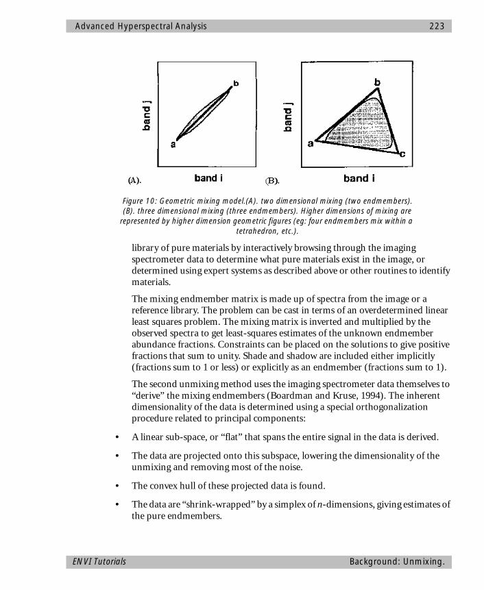
Advanced Hyperspectral Analysis 223
library of pure materials by interactively browsing through the imaging spectrometer data to determine what pure materials exist in the image, or determined using expert systems as described above or other routines to identify materials.
The mixing endmember matrix is made up of spectra from the image or a reference library. The problem can be cast in terms of an overdetermined linear least squares problem. The mixing matrix is inverted and multiplied by the observed spectra to get least-squares estimates of the unknown endmember abundance fractions. Constraints can be placed on the solutions to give positive fractions that sum to unity. Shade and shadow are included either implicitly (fractions sum to 1 or less) or explicitly as an endmember (fractions sum to 1).
The second unmixing method uses the imaging spectrometer data themselves to “derive” the mixing endmembers (Boardman and Kruse, 1994). The inherent dimensionality of the data is determined using a special orthogonalization procedure related to principal components:
• A linear sub-space, or “flat” that spans the entire signal in the data is derived.
• The data are projected onto this subspace, lowering the dimensionality of the unmixing and removing most of the noise.
• The convex hull of these projected data is found.
• The data are “shrink-wrapped” by a simplex of n-dimensions, giving estimates of the pure endmembers.
Figure 10: Geometric mixing model.(A). two dimensional mixing (two endmembers). (B). three dimensional mixing (three endmembers). Higher dimensions of mixing are
represented by higher dimension geometric figures (eg: four endmembers mix within a tetrahedron, etc.).
ENVI Tutorials Background: Unmixing.

224 Advanced Hyperspectral Analysis
• These derived endmembers must give feasible abundance estimates (positive fractions that sum to unity).
Spectral unmixing is one of the most promising hyperspectral analysis research areas. Analysis procedures using the convex geometry approach already developed for AVIRIS data have produced quantitative mapping results for a a variety of materials (geology, vegetation, oceanography) without a priori knowledge. Combination of the unmixing approach with model-based data calibration and expert system identification capabilities could potentially result in an end-to-end quantitative yet automated analysis methodology.
Unmixing ResultsIn this section, you will examine the results of unmixing using the means of the ROIs restored above and applied to the first ten MNF bands. You will then run your own unmixing using endmember suites of your own choosing.
Open and Display the Unmixing Results1. Open the file CUP95UNM.DAT.
2. Load the Kaolinite abundance image by clicking on the Kaolinite band name and then “Load Band” in the Available Bands List.
Brighter areas correspond to higher abundances.
• Use contrast stretching, if necessary, to show only the higher values (larger apparent abundances).
3. Load the other fractional abundance images into one or more displays and compare the distribution of endmembers.
Determine Abundances1. Select Basic Tools->Cursor Location/Value and investigate the values at
specific pixels.
2. Open the Effort data CUP95EFF.DAT and create spectral (Z) profiles of the reflectance data to reconcile absorption band strength with apparent abundance of the various endmembers.
Display a Color Composite1. Choose three good unmixing result images and make an RGB color
composite.
2. Use spatial and spectral clues to evaluate the results of the unmixing.
Unmixing Results ENVI Tutorials

Advanced Hyperspectral Analysis 225
3. Explain the colors in the RGB composite of fraction endmembers in terms of mixing.
Note the occurrence of non-primary colors (not R, G, or B).
• Are all of the fractions feasible?
Note areas where unreasonable results were obtained (eg. fractions greater than one or less than zero).
4. Examine the RMS Error image and look for areas with high errors (bright areas in the image).
• Are there other endmembers that could be used for iterative unmixing? How do you reconcile these results if the RMS Error image doesn’t have any high errors yet there are negative abundances or abundances greater than 1.0?
Optional: Perform Your Own Matched Filtering & Spectral Unmixing1. Choose Spectral Tools->Mapping Methods->Matched Filter or Linear
Spectral Unmixing.
You can create your own endmembers from single pixels, ROI means, or import them from spectral libraries.
Using the drag and drop method from spectral plots, you can build up your own spectral suite of mixing endmembers.
2. Click the right mouse button in the extreme right of the window that shows your desired endmember spectrum to view the spectrum name.
3. Click and drag on the spectrum name of the desired spectrum to move it.
4. Drop the name into the black box on the endmember selection dialog to add it to the suite of endmembers.
5. Compare your matched filter results and/or fractional abundance images to those previously examined.
Think about how the results depend entirely on the endmember selection.
Exit ENVI• When you have finished your ENVI session, click “Quit” or “Exit” on
the ENVI Main Menu.
ENVI Tutorials Unmixing Results
226 Advanced Hyperspectral Analysis
ReferencesBoardman, J. W., 1993, Automated spectral unmixing of AVIRIS data using convex geometry concepts: in Summaries, Fourth JPL Airborne Geoscience Workshop, JPL Publication 93-26, v. 1, p. 11 - 14.
Boardman J. W., and Kruse, F. A., 1994, Automated spectral analysis: A geologic example using AVIRIS data, north Grapevine Mountains, Nevada: in Proceedings, Tenth Thematic Conference on Geologic Remote Sensing, Environmental Research Institute of Michigan, Ann Arbor, MI, p. I-407 - I-418.
Boardman, J. W., Kruse, F. A., and Green, R. O., 1995, Mapping target signatures via partial unmixing of AVIRIS data: in Summaries, Fifth JPL Airborne Earth Science Workshop, JPL Publication 95-1, v. 1, p. 23-26.
Chen, J. Y., and Reed, I. S., 1987, A detection algorithm for optical targets in clutter, IEEE Trans. on Aerosp. Electron. Syst., vol. AES-23, no. 1.
Green, A. A., Berman, M., Switzer, P, and Craig, M. D., 1988, A transformation for ordering multispectral data in terms of image quality with implications for noise removal: IEEE Transactions on Geoscience and Remote Sensing, v. 26, no. 1, p. 65-74.
Harsanyi, J. C., and Chang, C. I., 1994, Hyperspectral image classification and dimensionality reduction: An orthogonal subspace projection approach: IEEE Trans. Geosci. and Remote Sens., v. 32, p. 779-785.
Nash, E. B., and Conel, J. E. (1974) Spectral reflectance systematics for mixtures of powdered hypersthene, labradorite, and ilmenite, Journal of Geophysical Research, 79, 1615-1621.
Singer, R. B., 1981, Near-infrared spectral reflectance of mineral mixtures: Systematic combinations of pyroxenes, olivine, and iron oxides: Journal of Geophysical Research, 86, 7967-7982.
Singer, R. B., and McCord, T. B., 1979, Mars: Large scale mixing of bright and dark surface materials and implications for analysis of spectral reflectance: in Proceedings Lunar and Planetary Science Conference, 10th, p. 1835-1848.
Stocker, A. D., Reed, I. S., and Yu, X., 1990, Mulitdimensional signal processing for electrooptical target detection, Proc, SPIE Int. Soc. Opt. Eng., vol. 1305
Yu, X., Reed, I. S., and Stocker, A. D., 1993, Comparative performance analysis of adaptive multispectral detectors, IEEE Trans. on Signal Processing, vol. 41, no. 8.
References ENVI Tutorials

ENVI Tutorial #11
Hyperpectral Signatures and Spectral ResolutionThe following topics are covered in this tutorial:
Overview of This Tutorial ......................................................................................228Files Used in This Tutorial ......................................................................................228Background ..........................................................................................................229Start ENVI .............................................................................................................233View Library Spectra .............................................................................................233View Landsat TM Image and Spectra ....................................................................234View GEOSCAN Data ............................................................................................235View GER63 Data ..................................................................................................237View AVIRIS Data ..................................................................................................239Evaluate Sensor Capabilities Vs ID Requirements ...................................................240Draw Conclusions .................................................................................................240Selected References of Interest ..............................................................................242
227
228 Hyperpectral Signatures and Spectral Resolution
Overview of This TutorialThis tutorial compares spectral resolution for several different sensors and the effect of resolution on the ability to discriminate and identify materials with distinct spectral signatures. The tutorial uses TM, GEOSCAN, GER63, and AVIRIS data from Cuprite, Nevada, USA, for intercomparison and comparison to materials from the USGS Spectral library.
Files Used in This TutorialYou must have the ENVI TUTORIALS & DATACD-ROM mounted on your system to access thefiles used by this tutorial, or copy the files to yourdisk.
Most of the files used in this tutorial are con-tained in the CUP_COMP subdirectory of theENVIDATA directory on the ENVI TUTORIALS& DATA CD-ROM. The AVIRIS reflectance im-age file CUP95EFF.INT, its associated ENVIheader file, and the extracted AVIRIS spectra arelocated in the C95AVSUB subdirectory.
Required FilesThe files listed below, along with their associated .hdr files, are required to run this exercise. Optional spectral library files listed below may also be used if more detailed comparisons are desired. Selected data files have been converted to integer format by multiplying the reflectance values by 1000 because of disk space considerations. Values of 1000 in the files represent reflectance values of 1.0.
Topics Covered in This Tutorial
Overview of This Tutorial
Files Used in This Tutorial
Background• Spectral Modeling and Resolution• Case History: Cuprite, Nevada,
USA
View Library Spectra• Plot selected spectra from the USGS
Spectral Library• Apply Scale Factor• Examine Spectral Features
View Landsat TM Data• Display image• Spectral Browsing using Z Profile• Compare to Library Spectra and other
instruments
View GEOSCAN Data• Display image• Spectral Browsing using Z Profile• Compare to Library Spectra and other
Instruments
View GER63 Data• Display image• Spectral Browsing using Z Profile• Compare to Library Spectra and other
Instruments
View AVIRIS Data• Display image• Spectral Browsing using Z Profile• Compare to Library Spectra and other
Instruments
Compare Spectral Resolution• Evaluate Sensor Capabilities Vs ID
Requirements• Draw Conclusions
References
Overview of This Tutorial ENVI Tutorials
Hyperpectral Signatures and Spectral Resolution 229
Required Files in the CUP_COMP DirectoryUSGS_EM.SLI Subset of USGS Spectral Library
USGS_EM.HDR ENVI Header for Above
CUPTM_RF.IMG Cuprite TM reflectance subset
CUPTM_RF.HDR ENVI Header for Above
CUPTM_EM.TXT Kaolinite and Alunite average spectra from above
CUPGS_SB.IMT Cuprite Geoscan Reflectance Image Subset
CUPGS_SB.HDR ENVI Header for above
CUPGS_TM.TXT Kaolinite and Alunite average spectra from above
CUPGERSB.IMG Cuprite GER64 Reflectance Image Subset
CUPGERSB.HDR ENVI Header for above
CUPGEREM.TXT Kaolinite and Alunite average spectra from above
Required Files in the C95AVSUB DirectoryCUP95EFF.INT Cuprite 1995 AVIRIS Reflectance Image Subset
(in the C95AVSUB directory)
CUP95EFF.HDR ENVI Header from above (in the C95AVSUB di-rectory)
CUP95EFF.TXT Kaolinite and Alunite average spectra from above in the C95AVSUB directory.
Optional Files (in the Default Spectral Library Directory)USGS_MIN.SLI USGS Spectral Library
USGS_MIN.HDR ENVI Header for Above
BackgroundSpectral resolution determines the way we see individual spectral features in materials measured using imaging spectrometry. Many people confuse the terms spectral resolution with spectral sampling. These are very different. Spectral resolution refers to the width of an instrument response (band-pass) at half of the band depth (the Full Width Half Max [FWHM]). Spectral sampling usually refers to the band spacing - the quantization of the spectrum at discrete steps - and may be very different from the spectral resolution. Quality spectrometers are usually designed so that the band spacing is about equal to the band FWHM, which is why band spacing is often thought of as equal to spectral resolution. These are two different things, however, so be careful in your use of terms.
ENVI Tutorials Background
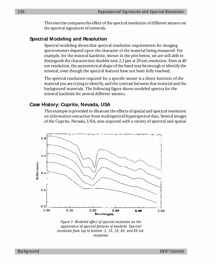
230 Hyperpectral Signatures and Spectral Resolution
This exercise compares the effect of the spectral resolution of different sensors on the spectral signatures of minerals.
Spectral Modeling and ResolutionSpectral modeling shows that spectral resolution requirements for imaging spectrometers depend upon the character of the material being measured. For example, for the mineral kaolinite, shown in the plot below, we are still able to distinguish the characteristic doublet near 2.2 µm at 20 nm resolution. Even at 40 nm resolution, the asymmetrical shape of the band may be enough to identify the mineral, even though the spectral features have not been fully resolved.
The spectral resolution required for a specific sensor is a direct function of the material you are trying to identify, and the contrast between that material and the background materials. The following figure shows modeled spectra for the mineral kaolinite for several different sensors.
Case History: Cuprite, Nevada, USAThis example is provided to illustrate the effects of spatial and spectral resolution on information extraction from multispectral/hyperspectral data. Several images of the Cuprite, Nevada, USA, area acquired with a variety of spectral and spatial
Figure 1: Modeled effect of spectral resolution on the appearance of spectral features of kaolinite. Spectral
resolution from top to bottom: 5, 10, 20, 40, and 80 nm resolution
Background ENVI Tutorials
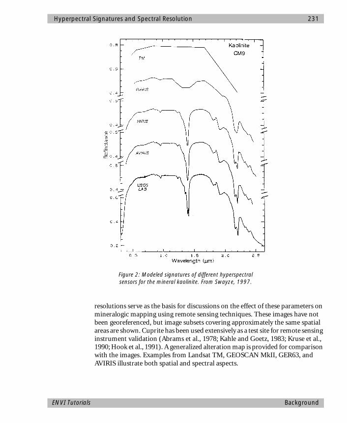
Hyperpectral Signatures and Spectral Resolution 231
resolutions serve as the basis for discussions on the effect of these parameters on mineralogic mapping using remote sensing techniques. These images have not been georeferenced, but image subsets covering approximately the same spatial areas are shown. Cuprite has been used extensively as a test site for remote sensing instrument validation (Abrams et al., 1978; Kahle and Goetz, 1983; Kruse et al., 1990; Hook et al., 1991). A generalized alteration map is provided for comparison with the images. Examples from Landsat TM, GEOSCAN MkII, GER63, and AVIRIS illustrate both spatial and spectral aspects.
Figure 2: Modeled signatures of different hyperspectral sensors for the mineral kaolinite. From Swayze, 1997.
ENVI Tutorials Background
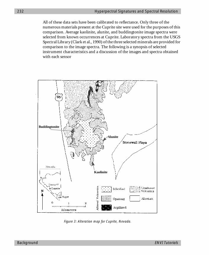
232 Hyperpectral Signatures and Spectral Resolution
All of these data sets have been calibrated to reflectance. Only three of the numerous materials present at the Cuprite site were used for the purposes of this comparison. Average kaolinite, alunite, and buddingtonite image spectra were selected from known occurrences at Cuprite. Laboratory spectra from the USGS Spectral Library (Clark et al., 1990) of the three selected minerals are provided for comparison to the image spectra. The following is a synopsis of selected instrument characteristics and a discussion of the images and spectra obtained with each sensor
Alunite
Kaolinite
Buddingtonite
Figure 3: Alteration map for Cuprite, Nevada.
Background ENVI Tutorials
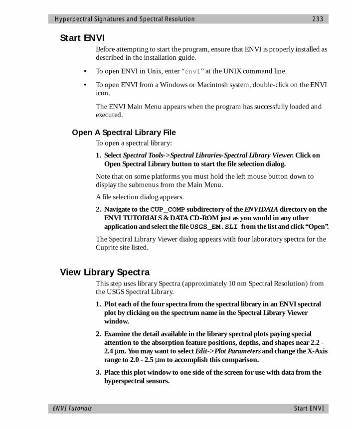
Hyperpectral Signatures and Spectral Resolution 233
Start ENVIBefore attempting to start the program, ensure that ENVI is properly installed as described in the installation guide.
• To open ENVI in Unix, enter “envi” at the UNIX command line.
• To open ENVI from a Windows or Macintosh system, double-click on the ENVI icon.
The ENVI Main Menu appears when the program has successfully loaded and executed.
Open A Spectral Library FileTo open a spectral library:
1. Select Spectral Tools->Spectral Libraries-Spectral Library Viewer. Click on Open Spectral Library button to start the file selection dialog.
Note that on some platforms you must hold the left mouse button down to display the submenus from the Main Menu.
A file selection dialog appears.
2. Navigate to the CUP_COMP subdirectory of the ENVIDATA directory on the ENVI TUTORIALS & DATA CD-ROM just as you would in any other application and select the file USGS_EM.SLI from the list and click “Open”.
The Spectral Library Viewer dialog appears with four laboratory spectra for the Cuprite site listed.
View Library SpectraThis step uses library Spectra (approximately 10 nm Spectral Resolution) from the USGS Spectral Library.
1. Plot each of the four spectra from the spectral library in an ENVI spectral plot by clicking on the spectrum name in the Spectral Library Viewer window.
2. Examine the detail available in the library spectral plots paying special attention to the absorption feature positions, depths, and shapes near 2.2 - 2.4 µm. You may want to select Edit->Plot Parameters and change the X-Axis range to 2.0 - 2.5 µm to accomplish this comparison.
3. Place this plot window to one side of the screen for use with data from the hyperspectral sensors.
ENVI Tutorials Start ENVI
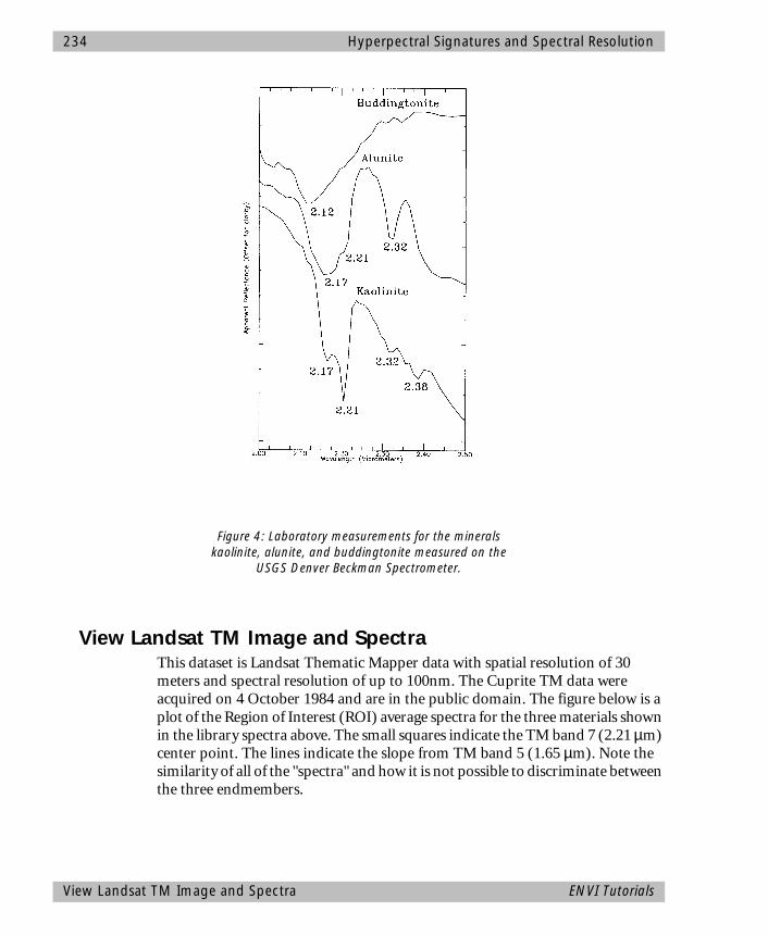
234 Hyperpectral Signatures and Spectral Resolution
View Landsat TM Image and SpectraThis dataset is Landsat Thematic Mapper data with spatial resolution of 30 meters and spectral resolution of up to 100nm. The Cuprite TM data were acquired on 4 October 1984 and are in the public domain. The figure below is a plot of the Region of Interest (ROI) average spectra for the three materials shown in the library spectra above. The small squares indicate the TM band 7 (2.21 µm) center point. The lines indicate the slope from TM band 5 (1.65 µm). Note the similarity of all of the "spectra" and how it is not possible to discriminate between the three endmembers.
USGS Lab
Figure 4: Laboratory measurements for the minerals kaolinite, alunite, and buddingtonite measured on the
USGS Denver Beckman Spectrometer.
View Landsat TM Image and Spectra ENVI Tutorials
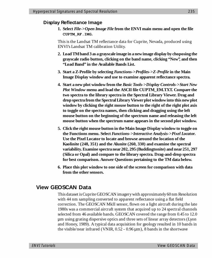
Hyperpectral Signatures and Spectral Resolution 235
Display Reflectance Image1. Select File->Open Image File from the ENVI main menu and open the file
CUPTM_RF.IMG.
This is the Landsat TM reflectance data for Cuprite, Nevada, produced using ENVI’s Landsat TM calibration Utility.
2. Load TM band 3 as a grayscale image in a new image display by choposing the grayscale radio button, clicking on the band name, clicking “New”, and then “Load Band” in the Available Bands List.
3. Start a Z-Profile by selecting Functions->Profiles->Z-Profile in the Main Image Display window and use to examine apparent reflectance spectra.
4. Start a new plot window from the Basic Tools->Display Controls->Start New Plot Window menu and load the ASCII file CUPTM_EM.TXT. Compare the two spectra to the library spectra in the Spectral Library Viewer. Drag and drop spectra from the Spectral Library Viewer plot window into this new plot window by clicking the right mouse button to the right of the right plot axis to toggle on the spectra names, then clicking and dragging using the left mouse button on the beginning of the spectrum name and releasing the left mouse button when the spectrum name appears in the second plot window.
5. Click the right mouse button in the Main Image Display window to toggle on the Functions menu. Select Functions->Interactive Analysis->Pixel Locator. Use the Pixel Locator to locate and browse around the location of the Kaolinite (248, 351) and the Alunite (260, 330) and examine the spectral variability. Examine spectra near 202, 295 (Buddingtonite) and near 251, 297 (Silica or Opal) and compare to the library spectra. Drag-and-drop spectra for best comparison. Answer Questions pertaining to the TM data below.
6. Place this plot window to one side of the screen for comparison with data from the other sensors.
View GEOSCAN DataThis dataset is Cuprite GEOSCAN imagery with approximately 60 nm Resolution with 44 nm sampling converted to apparent reflectance using a flat field correction. The GEOSCAN MkII sensor, flown on a light aircraft during the late 1980s was a commercial aircraft system that acquired up to 24 spectral channels selected from 46 available bands. GEOSCAN covered the range from 0.45 to 12.0 µm using grating dispersive optics and three sets of linear array detectors (Lyon and Honey, 1989). A typical data acquisition for geology resulted in 10 bands in the visible/near infrared (VNIR, 0.52 - 0.96 µm), 8 bands in the shortwave
ENVI Tutorials View GEOSCAN Data
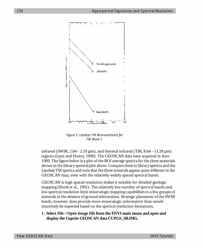
236 Hyperpectral Signatures and Spectral Resolution
infrared (SWIR, 2.04 - 2.35 µm), and thermal infrared (TIR, 8.64 - 11.28 µm) regions (Lyon and Honey, 1990). The GEOSCAN data were acquired in June 1989. The figure below is a plot of the ROI average spectra for the three materials shown in the library spectral plot above. Compare these to library spectra and the Landsat TM spectra and note that the three minerals appear quite different in the GEOSCAN data, even with the relatively widely spaced spectral bands.
GEOSCAN is high spatial resolution makes it suitable for detailed geologic mapping (Hook et al., 1991). The relatively low number of spectral bands and, low spectral resolution limit mineralogic mapping capabilities to a few groups of minerals in the absence of ground information. Strategic placement of the SWIR bands, however, does provide more mineralogic information than would intuitively be expected based on the spectral resolution limitations.
1. Select File->Open Image File from the ENVI main menu and open and display the Cuprite GEOSCAN data CUPGS_SB.IMG.
Figure 5: Landsat TM Measurements for TM Band 7.
View GEOSCAN Data ENVI Tutorials

Hyperpectral Signatures and Spectral Resolution 237
2. Start a Z-Profile by selecting Functions->Profiles->Z-Profile in the Main Image Display window and use to browse through some of the apparent reflectance spectra.
3. Load a color composite image of bands 13, 15, and 18 (RGB) to enhance mineralogical differences.
4. Start a new plot window from the Basic Tools->Display Controls->Start New Plot Window menu and load the ASCII file CUPGS_EM.TXT. Compare the two spectra to the library spectra in the Spectral Library Viewer, and to the spectra from the other sensors. Drag and drop spectra as described above for direct comparison.
5. Click the right mouse button in the Main Image Display window to toggle on the Functions menu. Select Functions->Interactive Analysis->Pixel Locator. Use the Pixel Locator to locate and browse around the location of the Kaolinite (275, 761) and the Alunite (435, 551) and examine the spectral variability. Examine spectra near 168, 475 (Buddingtonite) and near 371, 592 (Silica or Opal) and compare to the library spectra and spectra from the other sensors. Answer Questions pertaining to the GEOSCAN data below.
6. Place this plot window to one side of the screen for comparison with data from the other sensors.
View GER63 DataThis dataset is Cuprite Geophysical and Environmental Research 63-band scanner data (GER63). It has an advertised spectral resolution of 17.5 nm, but comparison with other sensors and laboratory spectra suggests that 35 nm resolution with 17.5 nm sampling is more likely. Four bad bands have been dropped so that only 59 spectral bands are available. The GER63 data described here were acquired during August 1987. Selected analysis results were previously published in Kruse et al. (1990). The figure below is a plot of the ROI average spectra for the three materials shown in the library spectra above. Note that the GER63 data adequately discriminate the alunite and buddingtonite, but do not fully resolve the kaolinite "doublet" near 2.2 µm shown in the laboratory.
1. Select File->Open Image File from the ENVI main menu and open and display the Cuprite GER64 data CUPGERSB.IMG.
2. Start a Z-Profile by selecting Functions->Profiles->Z-Profile in the Main Image Display window and use to browse through some of the apparent reflectance spectra.
ENVI Tutorials View GER63 Data
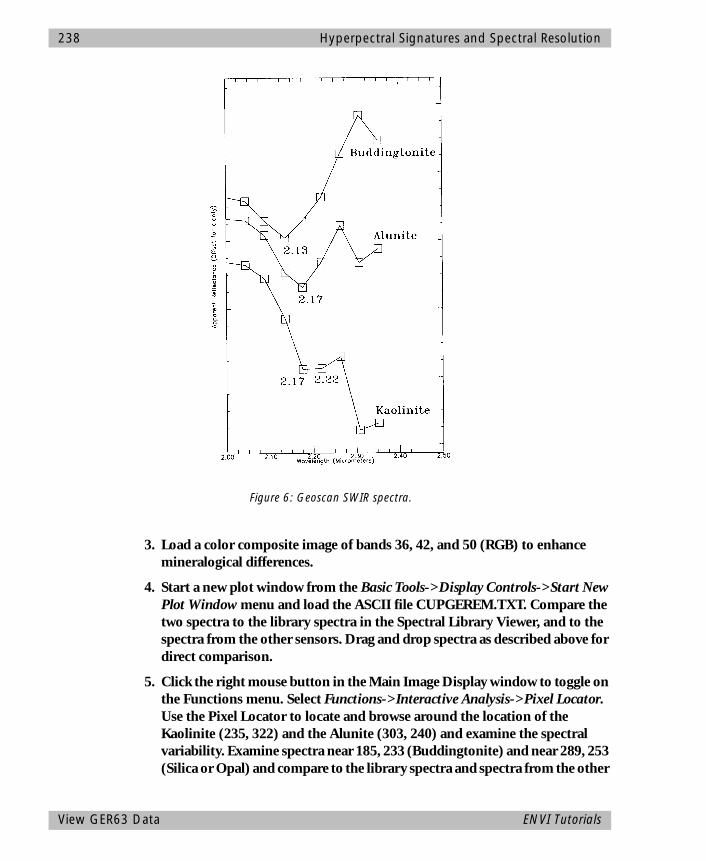
238 Hyperpectral Signatures and Spectral Resolution
3. Load a color composite image of bands 36, 42, and 50 (RGB) to enhance mineralogical differences.
4. Start a new plot window from the Basic Tools->Display Controls->Start New Plot Window menu and load the ASCII file CUPGEREM.TXT. Compare the two spectra to the library spectra in the Spectral Library Viewer, and to the spectra from the other sensors. Drag and drop spectra as described above for direct comparison.
5. Click the right mouse button in the Main Image Display window to toggle on the Functions menu. Select Functions->Interactive Analysis->Pixel Locator. Use the Pixel Locator to locate and browse around the location of the Kaolinite (235, 322) and the Alunite (303, 240) and examine the spectral variability. Examine spectra near 185, 233 (Buddingtonite) and near 289, 253 (Silica or Opal) and compare to the library spectra and spectra from the other
Figure 6: Geoscan SWIR spectra.
View GER63 Data ENVI Tutorials
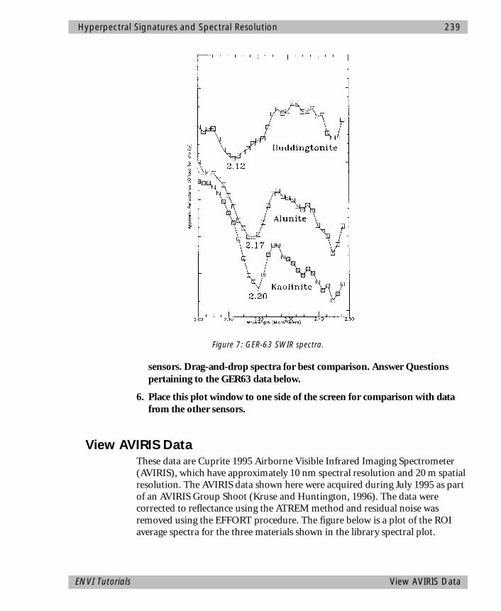
Hyperpectral Signatures and Spectral Resolution 239
sensors. Drag-and-drop spectra for best comparison. Answer Questions pertaining to the GER63 data below.
6. Place this plot window to one side of the screen for comparison with data from the other sensors.
View AVIRIS DataThese data are Cuprite 1995 Airborne Visible Infrared Imaging Spectrometer (AVIRIS), which have approximately 10 nm spectral resolution and 20 m spatial resolution. The AVIRIS data shown here were acquired during July 1995 as part of an AVIRIS Group Shoot (Kruse and Huntington, 1996). The data were corrected to reflectance using the ATREM method and residual noise was removed using the EFFORT procedure. The figure below is a plot of the ROI average spectra for the three materials shown in the library spectral plot.
Figure 7: GER-63 SWIR spectra.
ENVI Tutorials View AVIRIS Data

240 Hyperpectral Signatures and Spectral Resolution
Compare these to the laboratory spectra above and note the high quality and nearly identical signatures.
1. Select File->Open File and navigate to the C95AVSUB subdirectory of the ENVIDATA directory on the ENVI TUTORIALS & DATA CD-ROM just as you would in any other application and select the file CUP95EFF.INT from the list and click “OK”.
2. Display a grayscale image and then start a Z-Profile by selecting Functions->Profiles->Z-Profile in the Main Image Display window and use to browse through some of the apparent reflectance spectra.
3. Load a color composite image of bands 183, 193, and 207 (RGB) to enhance mineralogical differences.
4. Start a new plot window from the Basic Tools->Display Controls->Start New Plot Window menu and load the ASCII file CUP95EFF.TXT. Compare the two spectra to the library spectra in the Spectral Library Viewer, and to the spectra from the other sensors. Drag and drop spectra as described above for direct comparison.
5. Click the right mouse button in the Main Image Display window to toggle on the Functions menu. Select Functions->Interactive Analysis->Pixel Locator.Use the Pixel Locator to locate and browse around the location of the Kaolinite (500, 581) and the Alunite (538, 536) and examine the spectral variability. Examine spectra near 447, 484 (Buddingtonite) and 525, 505 (Silica or Opal) and compare to the library spectra and spectra from the other sensors. Drag-and-drop spectra for best comparison. Answer Questions pertaining to the 1995 AVIRIS data below.
Evaluate Sensor Capabilities Vs ID RequirementsThese four sensors and the library spectra represent a broad range of spectral resolutions.
1. Using the Library Spectra as the ground truth, evaluate how well each of the sensors is able to represent the ground truth information. Consider what it means to discriminate between materials versus identification of materials.
Draw Conclusions1. Using the selected library spectra provided, what is the minimum spacing of
absorption features in the 2.0 - 2.5 µm range?
Evaluate Sensor Capabilities Vs ID Requirements ENVI Tutorials
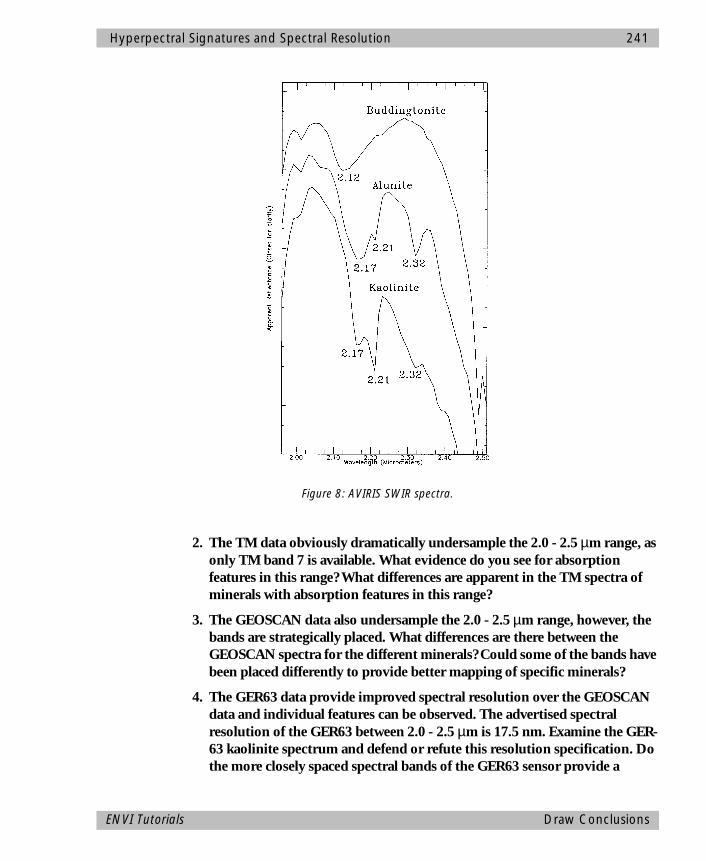
Hyperpectral Signatures and Spectral Resolution 241
2. The TM data obviously dramatically undersample the 2.0 - 2.5 µm range, as only TM band 7 is available. What evidence do you see for absorption features in this range? What differences are apparent in the TM spectra of minerals with absorption features in this range?
3. The GEOSCAN data also undersample the 2.0 - 2.5 µm range, however, the bands are strategically placed. What differences are there between the GEOSCAN spectra for the different minerals? Could some of the bands have been placed differently to provide better mapping of specific minerals?
4. The GER63 data provide improved spectral resolution over the GEOSCAN data and individual features can be observed. The advertised spectral resolution of the GER63 between 2.0 - 2.5 µm is 17.5 nm. Examine the GER-63 kaolinite spectrum and defend or refute this resolution specification. Do the more closely spaced spectral bands of the GER63 sensor provide a
Figure 8: AVIRIS SWIR spectra.
ENVI Tutorials Draw Conclusions
242 Hyperpectral Signatures and Spectral Resolution
significant advantage over the GEOSCAN data in mapping and identifying these reference minerals?
5. The AVIRIS data provide the best spectral resolution of the sensors examined here. How do the AVIRIS and laboratory spectra compare? What are the major similarities and differences? What factors affect the comparison of the two data types?
6. Examine all of the images and spectra. What role does spatial resolution play in the comparison?
7. Based on the Library spectra, provide sensor spectral and spatial resolution design specifications as well as recommendations on placement of spectral bands for mineral mapping. Examine the tradeoffs between continuous high-spectral resolution bands and strategically placed, lower resolution bands
Selected References of InterestAbrams, M. J., Ashley, R. P., Rowan, L. C., Goetz, A. F. H., and Kahle, A. B., 1978, Mapping of hydrothermal alteration in the Cuprite Mining District, Nevada using aircraft scanner images for the spectral region 0.46 - 2.36 mm: Geology, v. 5., p. 173 - 718.
Abrams, M., and Hook, S. J., 1995, Simulated ASTER data for Geologic Studies: IEEE Transactions on Geoscience and Remote Sensing, v. 33, no. 3, p. 692 - 699.
Chrien, T. G., Green, R. O., and Eastwood, M. L., 1990, Accuracy of the spectral and radiometric laboratory calibration of the Airborne Visible/Infrared Imaging Spectrometer: in Proceedings The International Society for Optical Engineering (SPIE), v. 1298, p. 37-49.
Clark, R. N., King, T. V. V., Klejwa, M., and Swayze, G. A., 1990, High spectral resolution spectroscopy of minerals: Journal of Geophysical Research, v. 95, no., B8, p. 12653 - 12680.
Clark, R. N., Swayze, G. A., Gallagher, A., King, T. V. V., and Calvin, W. M., 1993, The U. S. Geological Survey Digital Spectral Library: Version 1: 0.2 to 3.0 mm: U. S. Geological Survey, Open File Report 93-592, 1340 p.
CSES, 1992, Atmosphere REMoval Program (ATREM) User’s Guide, Version 1.1, Center for the Study of Earth from Space, Boulder, Colorado, 24 p.
Goetz, A. F. H., and Kindel, B., 1996, Understanding unmixed AVIRIS images in Cuprite, NV using coincident HYDICE data: in Summaries of the Sixth Annual JPL Airborne Earth Science Workshop, March 4-8, 1996, v. 1 (Preliminary).
Selected References of Interest ENVI Tutorials
Hyperpectral Signatures and Spectral Resolution 243
Goetz, A. F. H., and Rowan, L. C., 1981, Geologic Remote Sensing: Science, v. 211, p. 781 - 791.
Goetz, A. F. H., Rock, B. N., and Rowan, L. C., 1983, Remote Sensing for Exploration: An Overview: Economic Geology, v. 78, no. 4, p. 573 - 590.
Goetz, A. F. H., Vane, G., Solomon, J. E., and Rock , B. N., 1985, Imaging spectrometry for earth remote sensing: Science, v. 228, p. 1147 - 1153.
Green, R. O., Conel, J. E., Margolis, J., Chovit, C., and Faust, J., 1996, In-flight calibration and validation of the Airborne Visible/Infrared Imaging Spectrometer (AVIRIS): in Summaries of the Sixth Annual JPL Airborne Geoscience Workshop, 4-8 March 1996, Jet Propulsion Laboratory, Pasadena, CA, v. 1, (Preliminary).
Hook, S. J., Elvidge, C. D., Rast, M., and Watanabe, H., 1991, An evaluation of short-wave-infrared (SWIR) data from the AVIRIS and GEOSCAN instruments for mineralogic mapping at Cuprite, Nevada: Geophysics, v. 56, no. 9, p. 1432 - 1440.
Kruse, F. A., 1988, Use of Airborne Imaging Spectrometer data to map minerals associated with hydrothermally altered rocks in the northern Grapevine Mountains, Nevada and California: Remote Sensing of Environment, V. 24, No. 1, p. 31-51.
Kruse, F. A., and Huntington, J. H., 1996, The 1995 Geology AVIRIS Group Shoot: in Summaries of the Sixth Annual JPL Airborne Earth Science Workshop, March 4 - 8, 1996 Volume 1, AVIRIS Workshop, (Preliminary).
Kruse, F. A., Kierein-Young, K. S., and Boardman, J. W., 1990, Mineral mapping at Cuprite, Nevada with a 63 channel imaging spectrometer: Photogrammetric Engineering and Remote Sensing, v. 56, no. 1, p. 83-92.
Lyon, R. J. P., and Honey, F. R., 1989, spectral signature extraction from airborne imagery using the Geoscan MkII advanced airborne scanner in the Leonora, Western Australia Gold District: in IGARSS-89/12th Canadian Symposium on Remote Sensing, v. 5, p. 2925 - 2930.
Lyon, R.J. P., and Honey, F. R., 1990, Thermal Infrared imagery from the Geoscan Mark II scanner of the Ludwig Skarn, Yerington, NV: in Proceedings of the Second Thermal Infrared Multispectral Scanner (TIMS) Workshop.
Paylor, E. D., Abrams, M. J., Conel, J. E., Kahle, A. B., and Lang, H. R., 1985, Performance evaluation and geologic utility of Landsat-4 Thematic Mapper Data: JPL Publication 85-66, Jet Propulsion Laboratory, Pasadena, CA, 68 p.
Pease, C. B., 1990, Satellite imaging instruments: Principles, Technologies, and Operational Systems: Ellis Horwid, N.Y., 336 p.
ENVI Tutorials Selected References of Interest

244 Hyperpectral Signatures and Spectral Resolution
Porter, W. M., and Enmark, H. E., 1987, System overview of the Airborne Visible/Infrared Imaging Spectrometer (AVIRIS), in Proceedings, Society of Photo-Optical Instrumentation Engineers (SPIE), v. 834, p. 22-31.
Swayze, Gregg, 1997, The hydrothermal and structural history of the Cuprite Mining District, Southwestern Nevada: an integrated geological and geophysical approach: Unpublished Ph. D. Dissertation, University of Colorado, Boulder.
Selected References of Interest ENVI Tutorials

ENVI Tutorial #12
Vegetation Hyperspectral Analysis Case History
The following topics are covered in this tutorial:
Overview of This Tutorial ......................................................................................246Files Used in This Tutorial ......................................................................................246Tasks .....................................................................................................................248Jasper Ridge Background Materials........................................................................249AVIRIS Processing Flow..........................................................................................253
245
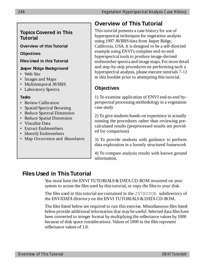
246 Vegetation Hyperspectral Analysis Case History
Overview of This TutorialThis tutorial presents a case history for use of hyperspectral techniques for vegetation analysis using 1997 AVIRIS data from Jasper Ridge, California, USA. It is designed to be a self-directed example using ENVI’s complete end-to-end hyperspectral tools to produce image-derived endmember spectra and image maps. For more detail and step-by-step procedures on performing such a hyperspectral analysis, please execute tutorials 7-11 in this booklet prior to attempting this tutorial.
Objectives
1) To examine application of ENVI end-to-end hy-perspectral processing methodology to a vegetationcase study
2) To give students hands-on experience in actuallyrunning the procedures rather than reviewing pre-calculated results (preprocessed results are provid-ed for comparison)
3) To provide students with guidance to performdata exploration in a loosely structured framework
4) To compare analysis results with known groundinformation.
Files Used in This TutorialYou must have the ENVI TUTORIALS & DATA CD-ROM mounted on your system to access the files used by this tutorial, or copy the files to your disk.
The files used in this tutorial are contained in the J97AVSUB subdirectory of the ENVIDATA directory on the ENVI TUTORIALS & DATA CD-ROM.
The files listed below are required to run this exercise. Miscellaneous files listed below provide additional information that may be useful. Selected data files have been converted to integer format by multiplying the reflectance values by 1000 because of disk space considerations. Values of 1000 in the files represent reflectance values of 1.0.
Topics Covered in This Tutorial
Overview of this Tutorial
Objectives
Files Used in this Tutorial
Jasper Ridge Background• Web Site• Images and Maps• Multitemporal AVIRIS• Laboratory Spectra
Tasks• Review Calibration• Spatial/Spectral Browsing• Reduce Spectral Dimension• Reduce Spatial Dimension• Visualize Data• Extract Endmembers• Identify Endmembers• Map Occurrence and Abundance
Overview of This Tutorial ENVI Tutorials
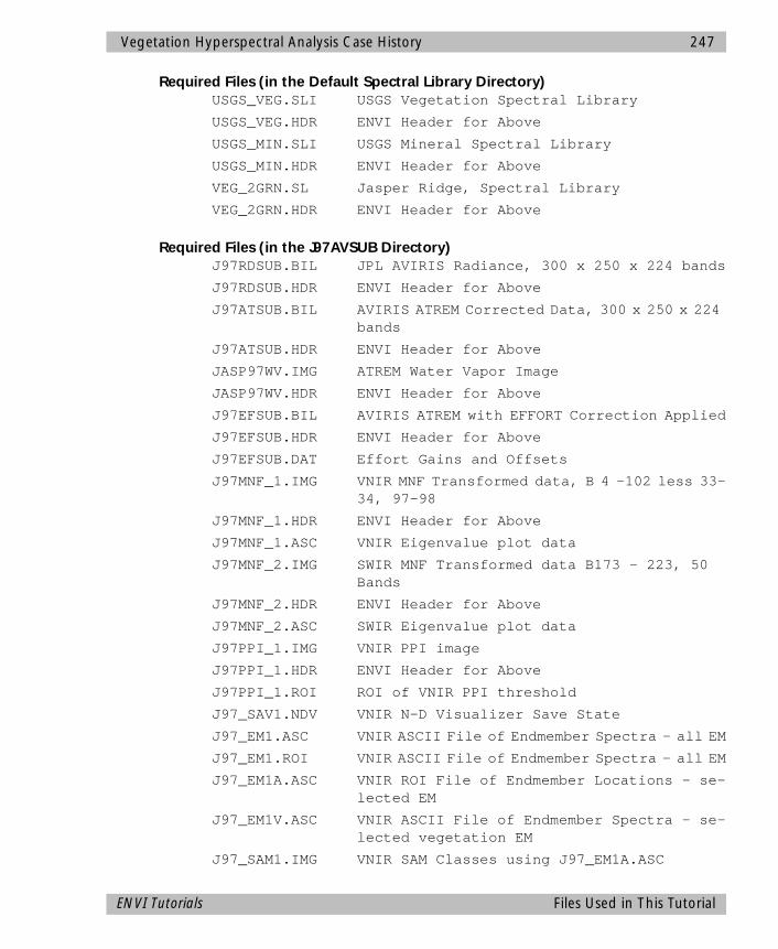
Vegetation Hyperspectral Analysis Case History 247
Required Files (in the Default Spectral Library Directory)USGS_VEG.SLI USGS Vegetation Spectral Library
USGS_VEG.HDR ENVI Header for Above
USGS_MIN.SLI USGS Mineral Spectral Library
USGS_MIN.HDR ENVI Header for Above
VEG_2GRN.SL Jasper Ridge, Spectral Library
VEG_2GRN.HDR ENVI Header for Above
Required Files (in the J97AVSUB Directory)J97RDSUB.BIL JPL AVIRIS Radiance, 300 x 250 x 224 bands
J97RDSUB.HDR ENVI Header for Above
J97ATSUB.BIL AVIRIS ATREM Corrected Data, 300 x 250 x 224 bands
J97ATSUB.HDR ENVI Header for Above
JASP97WV.IMG ATREM Water Vapor Image
JASP97WV.HDR ENVI Header for Above
J97EFSUB.BIL AVIRIS ATREM with EFFORT Correction Applied
J97EFSUB.HDR ENVI Header for Above
J97EFSUB.DAT Effort Gains and Offsets
J97MNF_1.IMG VNIR MNF Transformed data, B 4 -102 less 33-34, 97-98
J97MNF_1.HDR ENVI Header for Above
J97MNF_1.ASC VNIR Eigenvalue plot data
J97MNF_2.IMG SWIR MNF Transformed data B173 - 223, 50 Bands
J97MNF_2.HDR ENVI Header for Above
J97MNF_2.ASC SWIR Eigenvalue plot data
J97PPI_1.IMG VNIR PPI image
J97PPI_1.HDR ENVI Header for Above
J97PPI_1.ROI ROI of VNIR PPI threshold
J97_SAV1.NDV VNIR N-D Visualizer Save State
J97_EM1.ASC VNIR ASCII File of Endmember Spectra - all EM
J97_EM1.ROI VNIR ASCII File of Endmember Spectra - all EM
J97_EM1A.ASC VNIR ROI File of Endmember Locations - se-lected EM
J97_EM1V.ASC VNIR ASCII File of Endmember Spectra - se-lected vegetation EM
J97_SAM1.IMG VNIR SAM Classes using J97_EM1A.ASC
ENVI Tutorials Files Used in This Tutorial
248 Vegetation Hyperspectral Analysis Case History
J97_SAM1.HDR ENVI Header for Above
J97_RUL1.IMG VNIR SAM Rules
J97_RUL1.HDR ENVI Header for Above
J97SAM1V.IMG VNIR SAM Classes using J97_EM1V.ASC (vege-tation only)
J97SAM1V.HDR ENVI Header for Above
J97RUL1V.IMG VNIR SAM Rules Classes using J97_EM1V.ASC (vegetation only)
J97RUL1V.HDR ENVI Header for Above
J97_UNM1.IMG VNIR Linear Spectral Unmixing using J97_EM1.ASC
J97_UNM1.HDR ENVI Header for Above
J97PPI_2.IMG SWIR PPI image
J97PPI_2.HDR ENVI Header for Above
J7PPI_2.ROI ROI of SWIR PPI threshold
J97_SAV2.NDV SWIR N-D Visualizer Save State
J97_EM2.ASC SWIR ASCII File of all Endmember Spectra
J97_EM2A.ASC SWIR ASCII File of selected Endmember Spec-tra
J97_SAM2.IMG SWIR SAM Classes using J97_EM2A.ASC
J97_SAM2.HDR ENVI Header for Above
J97_RUL2.IMG SWIR SAM Rules
J97_RUL2.HDR ENVI Header for Above
J97_UNM2.IMG SWIR Linear Spectral Unmixing Results
J97_UNM2.HDR ENVI Header for Above
Other Miscellaneous Files (in the J97AVSUB Directory)JASP97.AVH JPL AVIRIS Header File
JASP97.WAV 1997 AVIRIS Wavelength file
JASP97.OCC JPL On-Board-Calibrator file
JASP97.SPC JPL Spectral Calibration File
JASP97.GN JPL DN-to-Radiance Gain File
Tasks1. Examine JPL AVIRIS radiance data and evaluate data characteristics and quality.
2. Evaluate Atmospherically Corrected (ATREM) AVIRIS data and compare to radiance data. Run and compare empirical correction methods.
Tasks ENVI Tutorials

Vegetation Hyperspectral Analysis Case History 249
3. Conduct Spatial/Spectral browsing to evaluate data, determine presence and nature of spectral variability, and to select wavelength range (s) for further analysis
4. Reduce data dimensionality using MNF transform
5. Select spectral endmember candidates using PPI
6. Evaluate linearity and select endmembers using n-D Visualizer
7. Map endmember distribution and abundance using ENVI mapping methods. Compare and contrast results
8. Reconcile image and field spectra/ground information
Jasper Ridge Background Materials
Remote Sensing Test Site Used By JPL and others since early 1980s
AVIRIS Standard Datasets for 1992-97
Detailed Maps and Ground Spectra Available.
ENVI Tutorials Jasper Ridge Background Materials
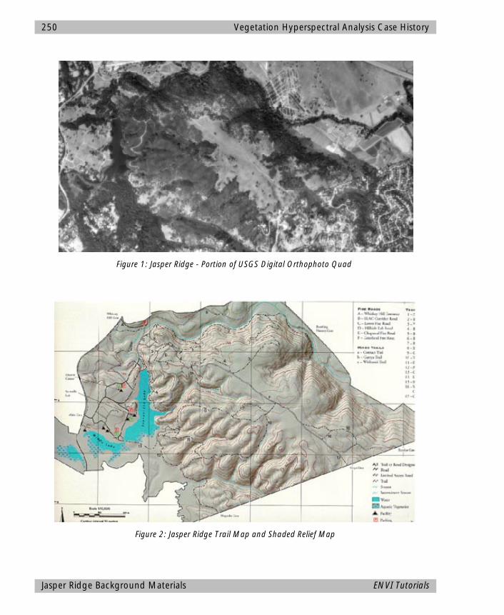
250 Vegetation Hyperspectral Analysis Case History
Figure 1: Jasper Ridge - Portion of USGS Digital Orthophoto Quad
Figure 2: Jasper Ridge Trail Map and Shaded Relief Map
Jasper Ridge Background Materials ENVI Tutorials
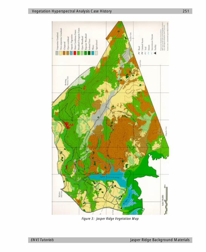
Vegetation Hyperspectral Analysis Case History 251
Figure 3: Jasper Ridge Vegetation Map
ENVI Tutorials Jasper Ridge Background Materials
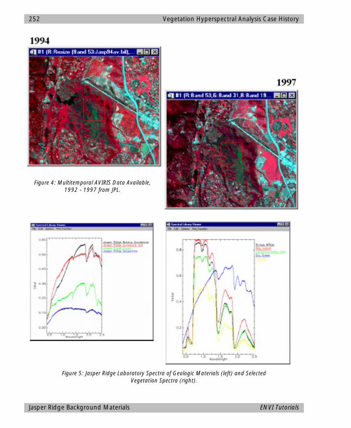
252 Vegetation Hyperspectral Analysis Case History
Figure 4: Multitemporal AVIRIS Data Available, 1992 - 1997 from JPL.
Figure 5: Jasper Ridge Laboratory Spectra of Geologic Materials (left) and Selected Vegetation Spectra (right).
Jasper Ridge Background Materials ENVI Tutorials
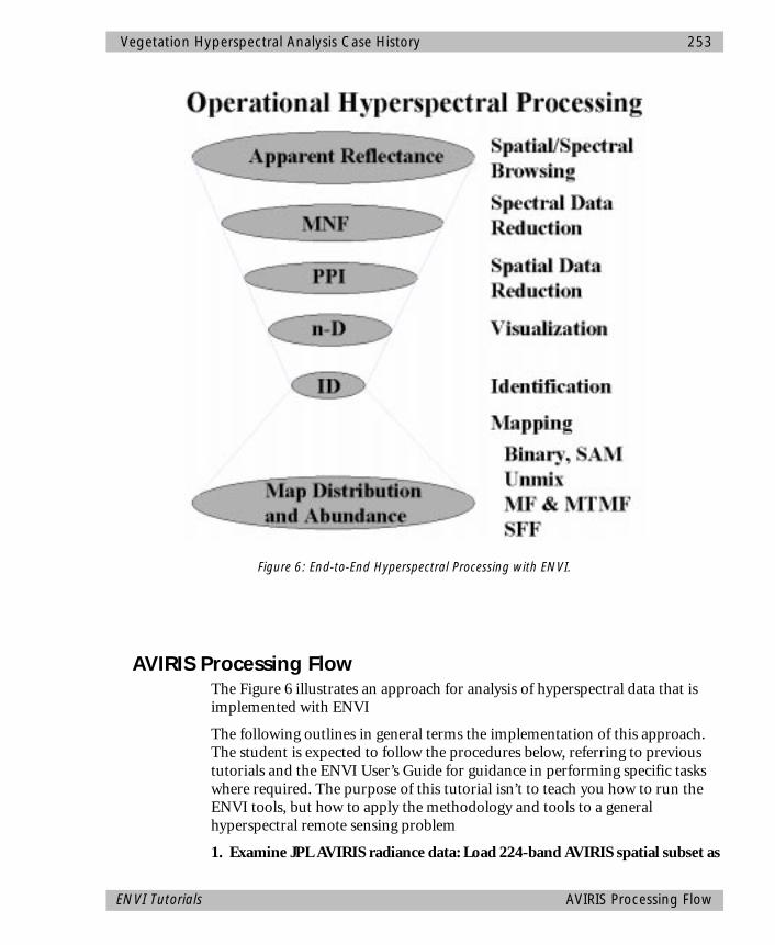
Vegetation Hyperspectral Analysis Case History 253
AVIRIS Processing FlowThe Figure 6 illustrates an approach for analysis of hyperspectral data that is implemented with ENVI
The following outlines in general terms the implementation of this approach. The student is expected to follow the procedures below, referring to previous tutorials and the ENVI User’s Guide for guidance in performing specific tasks where required. The purpose of this tutorial isn’t to teach you how to run the ENVI tools, but how to apply the methodology and tools to a general hyperspectral remote sensing problem
1. Examine JPL AVIRIS radiance data: Load 224-band AVIRIS spatial subset as
Figure 6: End-to-End Hyperspectral Processing with ENVI.
ENVI Tutorials AVIRIS Processing Flow
254 Vegetation Hyperspectral Analysis Case History
grayscale images. Perform animation. Extract radiance signatures for areas of high variability. Examine radiance spectra for evidence of absorption features. Determine bad spectral bands. Load color composite images designed to enhance spectral contrast. Determine spectral subset(s) to use for materials mapping for vegetation and/or minerals.
Files:
J97RDSUB.BIL JPL Radiance
2. Evaluate ATREM Correction applied to the JPL-provided AVIRIS spectral radiance to remove the bulk of the solar and atmospheric effects, transforming the data from radiance to apparent surface reflectance. Examine the data using spectral/spatial browsing and color composites to characterize spectral variability and determine residual errors. Review the water vapor image and relate to topography. Extract reflectance signatures for vegetation and geologic materials. Compare to spectral libraries.
Files:
J97ATSUB.BIL ATREM Apparent Reflectance
J97WVSUB.IMG ATREM Water Vapor Image
USGS_VEG.SLI Vegetation Spectral Library
USGS_MIN.SLI Mineral Spectral Library
VEG_2GRN.SL Jasper Ridge, Spectral Library
VEG_2GRN.HDR ENVI Header for Above
3. Evaluate EFFORT Correction applied to the ATREM data to remove residual errors. Review the gains and offsets used to make the correction using a plot window. Compare the EFFORT data to the ATREM apparent reflectance by examining the data using spectral/spatial browsing. Extract reflectance signatures for vegetation and geologic materials. Compare to spectral libraries.
Files:
J97EFSUB.BIL ATREM Apparent Reflectance with EFFORT Applied
J97EFSUB.DAT EFFORT Gains and Offsets
4. Apply MNF Transform to a spectral subset of the EFFORT data to find the data’s inherent dimensionality. Review MNF eigenvalue plot(s) to determine break-in-slope and relate to spatial coherency in MNF eigenimages. Determine MNF cut-off between "signal" and "noise" for further analysis.
Files: Make your own MNF-Transformed dataset or review the results in the files below
J97_MNF1.ASC VNIR Eigenvalue ASCII Data
AVIRIS Processing Flow ENVI Tutorials
Vegetation Hyperspectral Analysis Case History 255
JP7_MNF1.IMG VNIR MNF Eigenimages on 94 bands as listed above
J97_MNF2.ASC SWIR Eigenvalue ASCII Data
J97_MNF2.IMG SWIR MNF Eigenimages on 50 bands as listed above
5. Apply PPI Analysis to the MNF output to rank the pixels based on relative purity and spectral extremity. Use the FAST PPI option to perform calculations quickly in system memory, creating the PPI image. Display the PPI image, examine the histogram, and threshold to create a list of the purest pixels, spatially compressing the data.
Files: Generate your own PPI results and ROIs or review the results in the files below
J97PPI_1.IMG VNIR PPI Image
J97PPI_1.ROI VNIR PPI Threshold Results
J97PPI_2.IMG SWIR PPI Image
J97PPI_2.ROI SWIR PPI Threshold Results
6. Perform n-Dimensional Visualization of the high PPI value pixels, using the high signal MNF data bands to cluster the purest pixels into image-derived endmembers. Rotate the MNF data interactively in 3-D, or spin in 3-or-more dimensions and "paint" pixels that occur on the "points" (extremities) of the scatterplot. Use Z-Profiles connected to the EFFORT apparent reflectance data and the n-D Visualizer to evaluate spectral classes. Use class collapsing to iteratively find all of the endmembers. Evaluate the linearity of vegetation mixing and endmembers. Save your n-D results to a save state file (.ndv). Export classes to ROIs and extract mean spectra. Compare mean spectra to spectral libraries. Use spectral/spatial browsing to compare image spectra to ROI means.
Files: Extract endmembers and make your own ROIs or review the results below
J97_MNF1.IMG VNIR MNF Eigenimages on 94 bands as listed above
J97_MNF2.IMG SWIR MNF Eigenimages on 50 bands as listed above
J97EFSUB.BIL ATREM Apparent Reflectance with EFFORT Ap-plied
J97_SAV1.NDV VNIR n-d visualizer saved state
J97_SAV2.NDV SWIR n-d visualizer saved state
J97_EM1.ASC VNIR Saved ASCII Endmember Spectra
J97_EM2.ASC SWIR Saved ASCII Endmember Spectra
ENVI Tutorials AVIRIS Processing Flow
256 Vegetation Hyperspectral Analysis Case History
USGS_VEG.SLI Vegetation Spectral Library
USGS_MIN.SLI Mineral Spectral Library
VEG_2GRN.SL Jasper Ridge, Spectral Library
VEG_2GRN.HDR ENVI Header for Above
7. Use ENVI’s wide variety of mapping methods to map the spatial occurrence and abundance of materials at Jasper Ridge. As a minimum, try the Spectral Angle Mapper (SAM) and Unconstrained Linear Unmixing. Use SAM to determine spectral similarity to image endmember spectra Perform your own SAM Classification or review the results below. If time and space permit, try a SAM classification using one of the Spectral Libraries. Be sure to evaluate the Rule Images. Use the Unconstrained Linear Unmixing to determine material abundances. Be sure to examine the RMS error image and evaluate whether the physical constrains of non-negative and sum to unity (1) or less have been satisfied. Iterate if time and space permit. Compare abundance image results to the endmember spectra and spectral libraries using spatial/spectral browsing. If time and space permit, try running Mixture-Tuned Matched filtering and/or Spectral Feature Fitting.
Files:
J97_EM1.ASC VNIR Saved ASCII Endmember Spectra
J97_EM2.ASC SWIR Saved ASCII Endmember Spectra
J97EFSUB.BIL ATREM Apparent Reflectance with EFFORT Applied
J97_SAM1.IMG VNIR SAM Classes
J97_RUL1.IMG VNIR SAM Rules
J97_UNM1.IMG VNIR Linear Spectral Unmixing Results
J97_SAM1.IMG SWIR SAM Classes
J97_RUL1.IMG SWIR SAM Rules
J97_UNM1.IMG SWIR Linear Spectral Unmixing Results
USGS_VEG.SLI Vegetation Spectral Library
USGS_MIN.SLI Mineral Spectral Library
VEG_2GRN.SL Jasper Ridge, Spectral Library
VEG_2GRN.HDR ENVI Header for Above
AVIRIS Processing Flow ENVI Tutorials
ENVI Tutorial #13
Near-Shore Marine Hyperspectral Case History
The following topics are covered in this tutorial:
Overview of This Tutorial ......................................................................................258Objectives.............................................................................................................258Files Used in This Tutorial ......................................................................................258Tasks .....................................................................................................................259Moffett Field Site Background ...............................................................................260AVIRIS Processing Flow..........................................................................................261Selected References ..............................................................................................265
257
258 Near-Shore Marine Hyperspectral Case History
Overview of This TutorialThis tutorial presents a case history for use of hyperspectral techniques for vegetation analysis using 1994 AVIRIS data from Moffett Field, California, USA. It is designed to be a self-directed example using ENVI’s complete end-to-end hyperspectral tools to produce image-derived endmember spectra and image maps. For more detail and step-by-step procedures on performing such a hyperspectral analysis, please execute tutorials 7-11 in this booklet prior to attempting this tutorial.
Objectives
1) To examine application of ENVI end-to-end hy-perspectral processing methodology to a near-shoremarine case study
2) To give students hands-on experience in actuallyrunning the procedures rather than reviewing pre-calculated results (preprocessed results are provid-ed for comparison)
3) To provide students with guidance to performdata exploration in a loosely structured framework
4) To compare analysis results with known groundinformation.
Files Used in This TutorialYou must have the ENVI TUTORIALS & DATA CD-ROM mounted on your system to access the files used by this tutorial, or copy the files to your disk.
The files used in this tutorial are contained in the M94AVSUB subdirectory of the ENVIDATA directory on the ENVI TUTORIALS & DATA CD-ROM.
The files listed below are required to run this exercise. Selected data files have been converted to integer format by multiplying the reflectance values by 1000 because of disk space considerations. Values of 1000 in the files represent reflectance values of 1.0.
Required Files (in the Default Spectral Library Directory)USGS_VEG.SLI USGS Vegetation Spectral Library
USGS_VEG.HDR ENVI Header for Above
Topics Covered in This Tutorial
Overview of this Tutorial
Objectives
Files Used in this Tutorial
Moffett Dataset Background
Tasks• Review Calibration• Spatial/Spectral Browsing• Reduce Spectral Dimensions• Reduce Spatial Dimensions• Visualize Data• Evaluate Linearity• Extract Endmembers• Identify Endmembers• Map Occurrence and Abundance
Overview of This Tutorial ENVI Tutorials
Near-Shore Marine Hyperspectral Case History 259
USGS_MIN.SLI USGS Mineral Spectral Library
USGS_MIN.HDR ENVI Header for Above
Required Files (in the M97AVSUB Directory)M94AV.BIL AVIRIS ATREM Corrected Data, 500 x 350 x 56
bands
M94AV.HDR ENVI Header for Above
M94MNF.IMG VNIR MNF Transformed data
M94MNF.HDR ENVI Header for Above
M94MNF.ASC VNIR Eigenvalue plot data
M94PPI.IMG VNIR PPI image
M94PPI.HDR ENVI Header for Above
M94PPI.ROI ROI of VNIR PPI threshld
M94_EM.ASC VNIR ASCII File of Endmember Spectra - all EM
M94_EM.ROI VNIR ROI File of Endmember Spectra - all EM
M94_EMA.ASC VNIR ASCII File of Endmember Locations - se-lected EM
M94_SAM1.IMG VNIR SAM Classes using M94EM1A.ASC
M94_SAM1.HDR ENVI Header for Above
M94_RUL1.IMG VNIR SAM Rules
M94_RUL1.HDR ENVI Header for Above
M94_UNM1.IMG VNIR Unmixing image using M94EM1A.ASC
M94_UNM1.HDR ENVI Header for above
Tasks1. Examine ATREM-corrected apparent reflectance data and evaluate data
characteristics and quality.
2. Conduct Spatial/Spectral browsing to evaluate data, determine presence and nature of spectral variability, determine linearity of mixing, and to select wavelength range (s) for further analysis
3. Reduce data dimensionality using MNF transform
4. Select spectral endmember candidates using PPI
5. Evaluate linearity and select endmembers using n-D Visualizer
6. Map endmember distribution and abundance using ENVI mapping methods.
ENVI Tutorials Overview of This Tutorial

260 Near-Shore Marine Hyperspectral Case History
Moffett Field Site Background
• Launch site for AVIRIS at Moffett Field
• Remote Sensing Test Site Used By JPL and others since launch of AVIRIS in 1987
• AVIRIS Standard Datasets for 1992-97
• Study area for water variability (salt evaporation ponds with algae), urban studies, vegetation.
The salt ponds are highly colored and contain a dense biomass of algae and/or photosynthetic bacteria (Richardson et al., 1994). Accessory bacterial pigments cause distinct spectral signatures that can be detected using AVIRIS data. These include carotenoids, phycocyanin, and cholorphyll a and b. Application of the standardized AVIRIS analysis methods described below should lead to the extraction of endmembers from the data and spatial mapping of their distribution and abundance. There are obvious mixing non-linearities in the data, however, and care must be taken to recognize these.
Figure 1: 1994 Moffett Field AVIRIS Data.
Moffett Field Site Background ENVI Tutorials
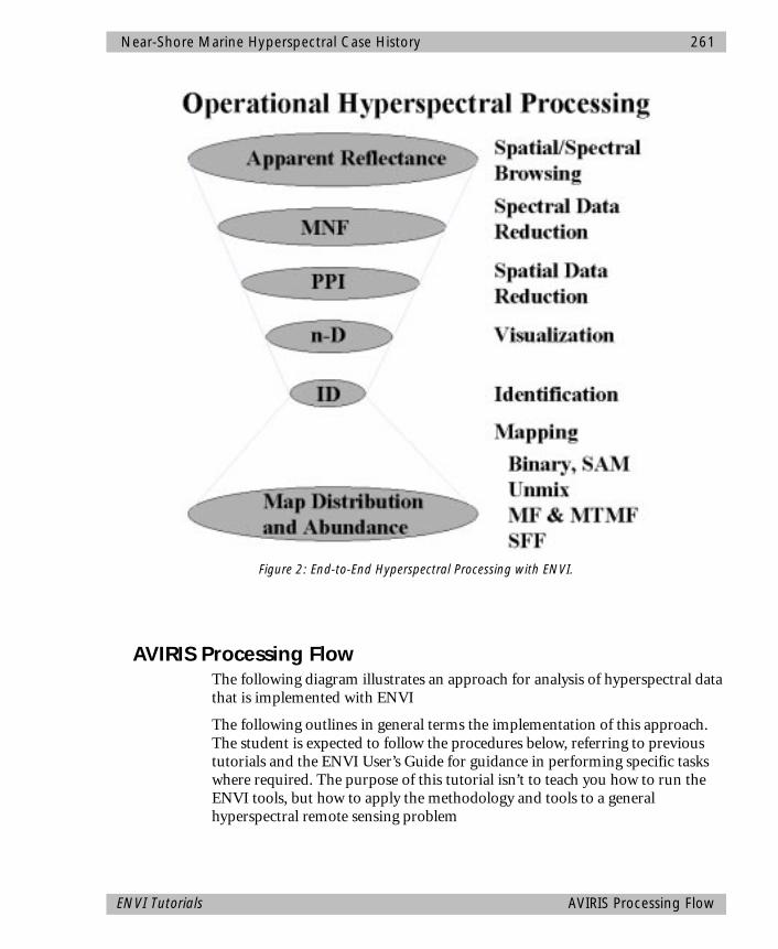
Near-Shore Marine Hyperspectral Case History 261
AVIRIS Processing FlowThe following diagram illustrates an approach for analysis of hyperspectral data that is implemented with ENVI
The following outlines in general terms the implementation of this approach. The student is expected to follow the procedures below, referring to previous tutorials and the ENVI User’s Guide for guidance in performing specific tasks where required. The purpose of this tutorial isn’t to teach you how to run the ENVI tools, but how to apply the methodology and tools to a general hyperspectral remote sensing problem
Figure 2: End-to-End Hyperspectral Processing with ENVI.
ENVI Tutorials AVIRIS Processing Flow
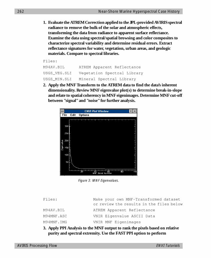
262 Near-Shore Marine Hyperspectral Case History
1. Evaluate the ATREM Correction applied to the JPL-provided AVIRIS spectral radiance to remove the bulk of the solar and atmospheric effects, transforming the data from radiance to apparent surface reflectance. Examine the data using spectral/spatial browsing and color composites to characterize spectral variability and determine residual errors. Extract reflectance signatures for water, vegetation, urban areas, and geologic materials. Compare to spectral libraries.
Files:
M94AV.BIL ATREM Apparent Reflectance
USGS_VEG.SLI Vegetation Spectral Library
USGS_MIN.SLI Mineral Spectral Library
2. Apply the MNF Transform to the ATREM data to find the data’s inherent dimensionality. Review MNF eigenvalue plot(s) to determine break-in-slope and relate to spatial coherency in MNF eigenimages. Determine MNF cut-off between "signal" and "noise" for further analysis.
Files: Make your own MNF-Transformed dataset or review the results in the files below
M94AV.BIL ATREM Apparent Reflectance
M94MNF.ASC VNIR Eigenvalue ASCII Data
M94MNF.IMG VNIR MNF Eigenimages
3. Apply PPI Analysis to the MNF output to rank the pixels based on relative purity and spectral extremity. Use the FAST PPI option to perform
Figure 3: MNF Eigenvalues.
AVIRIS Processing Flow ENVI Tutorials
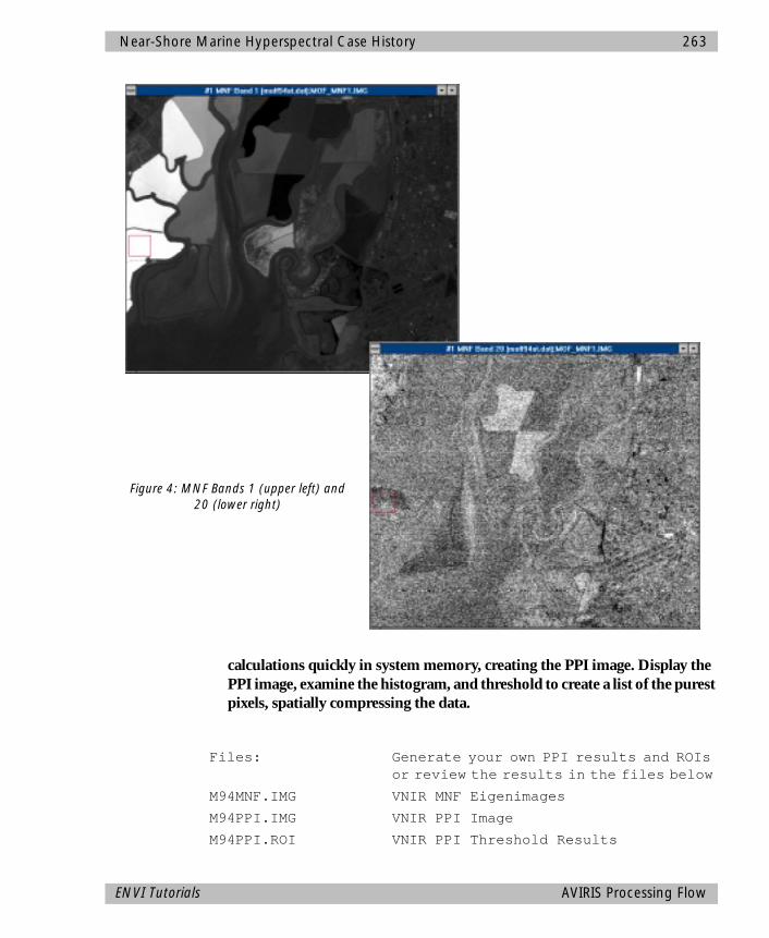
Near-Shore Marine Hyperspectral Case History 263
calculations quickly in system memory, creating the PPI image. Display the PPI image, examine the histogram, and threshold to create a list of the purest pixels, spatially compressing the data.
Files: Generate your own PPI results and ROIs or review the results in the files below
M94MNF.IMG VNIR MNF Eigenimages
M94PPI.IMG VNIR PPI Image
M94PPI.ROI VNIR PPI Threshold Results
Figure 4: MNF Bands 1 (upper left) and 20 (lower right)
ENVI Tutorials AVIRIS Processing Flow
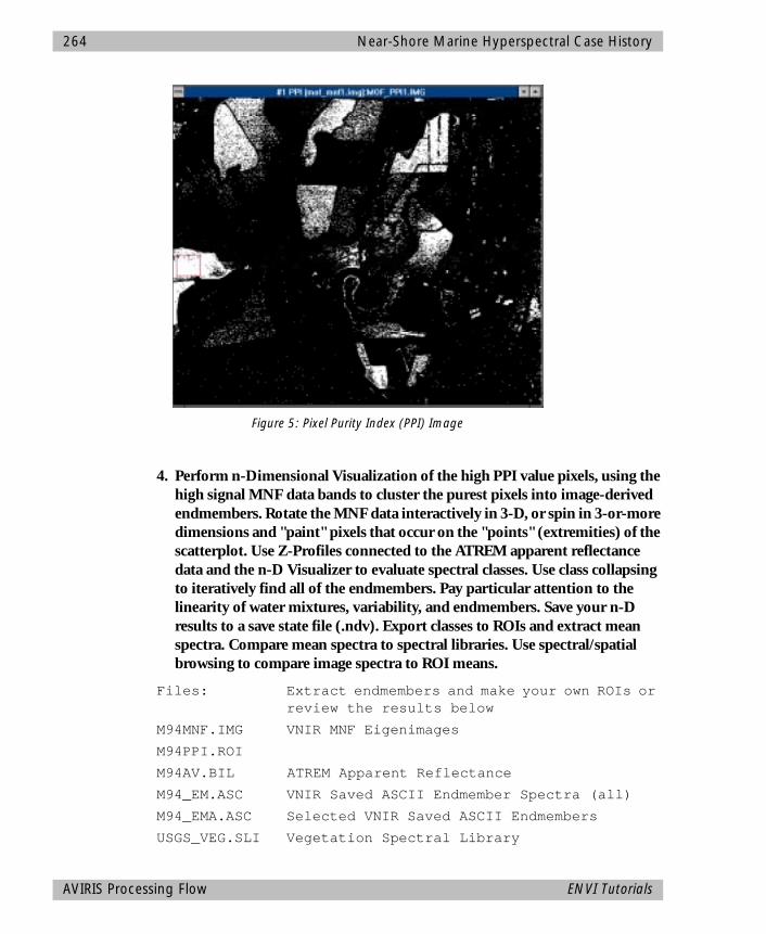
264 Near-Shore Marine Hyperspectral Case History
4. Perform n-Dimensional Visualization of the high PPI value pixels, using the high signal MNF data bands to cluster the purest pixels into image-derived endmembers. Rotate the MNF data interactively in 3-D, or spin in 3-or-more dimensions and "paint" pixels that occur on the "points" (extremities) of the scatterplot. Use Z-Profiles connected to the ATREM apparent reflectance data and the n-D Visualizer to evaluate spectral classes. Use class collapsing to iteratively find all of the endmembers. Pay particular attention to the linearity of water mixtures, variability, and endmembers. Save your n-D results to a save state file (.ndv). Export classes to ROIs and extract mean spectra. Compare mean spectra to spectral libraries. Use spectral/spatial browsing to compare image spectra to ROI means.
Files: Extract endmembers and make your own ROIs or review the results below
M94MNF.IMG VNIR MNF Eigenimages
M94PPI.ROI
M94AV.BIL ATREM Apparent Reflectance
M94_EM.ASC VNIR Saved ASCII Endmember Spectra (all)
M94_EMA.ASC Selected VNIR Saved ASCII Endmembers
USGS_VEG.SLI Vegetation Spectral Library
Figure 5: Pixel Purity Index (PPI) Image
AVIRIS Processing Flow ENVI Tutorials
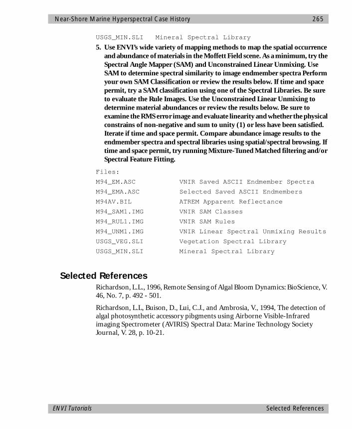
Near-Shore Marine Hyperspectral Case History 265
USGS_MIN.SLI Mineral Spectral Library
5. Use ENVI’s wide variety of mapping methods to map the spatial occurrence and abundance of materials in the Moffett Field scene. As a minimum, try the Spectral Angle Mapper (SAM) and Unconstrained Linear Unmixing. Use SAM to determine spectral similarity to image endmember spectra Perform your own SAM Classification or review the results below. If time and space permit, try a SAM classification using one of the Spectral Libraries. Be sure to evaluate the Rule Images. Use the Unconstrained Linear Unmixing to determine material abundances or review the results below. Be sure to examine the RMS error image and evaluate linearity and whether the physical constrains of non-negative and sum to unity (1) or less have been satisfied. Iterate if time and space permit. Compare abundance image results to the endmember spectra and spectral libraries using spatial/spectral browsing. If time and space permit, try running Mixture-Tuned Matched filtering and/or Spectral Feature Fitting.
Files:
M94_EM.ASC VNIR Saved ASCII Endmember Spectra
M94_EMA.ASC Selected Saved ASCII Endmembers
M94AV.BIL ATREM Apparent Reflectance
M94_SAM1.IMG VNIR SAM Classes
M94_RUL1.IMG VNIR SAM Rules
M94_UNM1.IMG VNIR Linear Spectral Unmixing Results
USGS_VEG.SLI Vegetation Spectral Library
USGS_MIN.SLI Mineral Spectral Library
Selected ReferencesRichardson, L.L., 1996, Remote Sensing of Algal Bloom Dynamics: BioScience, V. 46, No. 7, p. 492 - 501.
Richardson, L.L, Buison, D., Lui, C.J., and Ambrosia, V., 1994, The detection of algal photosynthetic accessory pibgments using Airborne Visible-Infrared imaging Spectrometer (AVIRIS) Spectral Data: Marine Technology Society Journal, V. 28, p. 10-21.
ENVI Tutorials Selected References
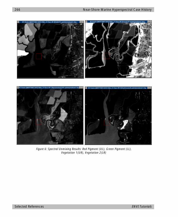
266 Near-Shore Marine Hyperspectral Case History
Figure 6: Spectral Unmixing Results: Red Pigment (UL), Green Pigment (LL), Vegetation 1(UR), Vegetation 2(LR)
Selected References ENVI Tutorials
ENVI Tutorial #14
Multispectral Processing using ENVI’s Hyperspectral Tools
The following topics are covered in this tutorial:
Overview of This Tutorial ......................................................................................268Background ..........................................................................................................268Files Used in This Tutorial ......................................................................................269Standard (Classical) Multispectral Image Processing..............................................270Application of ENVI’S Hyperspectral Tools to Multispectral Data Analysis ...............276Summary ..............................................................................................................292References ............................................................................................................292
267

268 Multispectral Processing using ENVI’s Hyperspectral Tools
Overview of This TutorialThis tutorial is designed to show you how ENVI’s advanced hyperspectral tools can be used for analysis of multispectral data. To gain a better understanding of the hyperspectral concepts and tools, please see the ENVI hyperspectral tutorials. For additional details, please see the ENVI User’s Guide or the ENVI On-Line help.
BackgroundENVI was not designed solely as a hyperspectral image processing system. The decision was made in 1992 to develop a general purpose image processing software package with a full suite of standard tools in response to the general lack of powerful yet flexible commercial products capable of handling a wide variety of scientific image data formats. This included support for panchromatic, multispectral, hyperspectral, and both basic and advanced radar systems. ENVI presently contains most of the same basic capabilities as other major image processing systems such as ERDAS, ERMapper, and PCI. Where ENVI differs is in the many advanced, state-of-the-art algorithms resulting from active leading-edge remote sensing research. While many of these features were developed specifically to deal with imaging spectrometer data or “hyperspectral” data having up to hundreds of spectral bands, many of these techniques are applicable to multispectral data and other standard data types. This tutorial presents a scenario for use of some of these methods for analysis of Landsat Thematic Mapper data.
This example is broken into two portions: 1) a typical multispectral analysis of TM data using “standard” or classical multispectral analysis techniques, and 2) analysis of the same dataset using ENVI's hyperspectral tools.
Topics Covered in This Tutorial
Overview of This Tutorial
Background
Files Used in this Tutorial
Standard (Classical) Multispectral Image Processing• Read TM Tape or CD• Display a Color Composite
Image• Conduct a Ratio Analysis• Run Supervised Classification
(IsoData)• Clump and Sieve, Combine
Classes• Annotate and Output Map
Application of ENVI’s Hyperspectral Tools to Multispectral Data Analysis• Calibrate TM Data to
Reflectance• Display a Color Composite
Image and Extract Spectra• Run Minimum Noise Fraction
(MNF) Transformation• Run PPI to Find Endmembers• n-D Visualization and Extract
Endmembers• Compare Image Spectra to
Spectral Library• Spectral Angle Mapper
Classification• Linear Spectral Unmixing• Annotate and Output Map
Summary
Overview of This Tutorial ENVI Tutorials
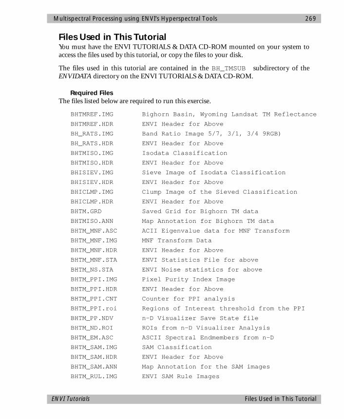
Multispectral Processing using ENVI’s Hyperspectral Tools 269
Files Used in This TutorialYou must have the ENVI TUTORIALS & DATA CD-ROM mounted on your system toaccess the files used by this tutorial, or copy the files to your disk.
The files used in this tutorial are contained in the BH_TMSUB subdirectory of theENVIDATA directory on the ENVI TUTORIALS & DATA CD-ROM.
Required FilesThe files listed below are required to run this exercise.
BHTMREF.IMG Bighorn Basin, Wyoming Landsat TM Reflectance
BHTMREF.HDR ENVI Header for Above
BH_RATS.IMG Band Ratio Image 5/7, 3/1, 3/4 9RGB)
BH_RATS.HDR ENVI Header for Above
BHTMISO.IMG Isodata Classification
BHTMISO.HDR ENVI Header for Above
BHISIEV.IMG Sieve Image of Isodata Classification
BHISIEV.HDR ENVI Header for Above
BHICLMP.IMG Clump Image of the Sieved Classification
BHICLMP.HDR ENVI Header for Above
BHTM.GRD Saved Grid for Bighorn TM data
BHTMISO.ANN Map Annotation for Bighorn TM data
BHTM_MNF.ASC ACII Eigenvalue data for MNF Transform
BHTM_MNF.IMG MNF Transform Data
BHTM_MNF.HDR ENVI Header for Above
BHTM_MNF.STA ENVI Statistics File for above
BHTM_NS.STA ENVI Noise statistics for above
BHTM_PPI.IMG Pixel Purity Index Image
BHTM_PPI.HDR ENVI Header for Above
BHTM_PPI.CNT Counter for PPI analysis
BHTM_PPI.roi Regions of Interest threshold from the PPI
BHTM_PP.NDV n-D Visualizer Save State file
BHTM_ND.ROI ROIs from n-D Visualizer Analysis
BHTM_EM.ASC ASCII Spectral Endmembers from n-D
BHTM_SAM.IMG SAM Classification
BHTM_SAM.HDR ENVI Header for Above
BHTM_SAM.ANN Map Annotation for the SAM images
BHTM_RUL.IMG ENVI SAM Rule Images
ENVI Tutorials Files Used in This Tutorial
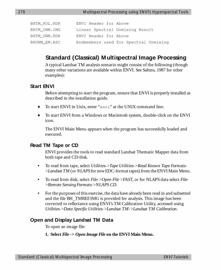
270 Multispectral Processing using ENVI’s Hyperspectral Tools
BHTM_RUL.HDR ENVI Header for Above
BHTM_UNM.IMG Linear Spectral Unmixing Result
BHTM_UNM.HDR ENVI Header for Above
BHUNM_EM.ASC Endmembers used for Spectral Unmixing
Standard (Classical) Multispectral Image Processing A typical Landsat TM analysis scenario might consist of the following (though many other variations are available within ENVI. See Sabins, 1987 for other examples):
Start ENVIBefore attempting to start the program, ensure that ENVI is properly installed as described in the installation guide.
♦ To start ENVI in Unix, enter “envi” at the UNIX command line.
♦ To start ENVI from a Windows or Macintosh system, double-click on the ENVI icon.
The ENVI Main Menu appears when the program has successfully loaded and executed.
Read TM Tape or CDENVI provides the tools to read standard Landsat Thematic Mapper data from both tape and CD/disk.
• To read from tape, select Utilities->Tape Utilities->Read Known Tape Formats->Landsat TM (or NLAPS for new EDC-format tapes) from the ENVI Main Menu.
• To read from disk, select File->Open File >FAST, or for NLAPS data select File->Remote Sensing Formats->NLAPS CD.
• For the purposes of this exercise, the data have already been read in and subsetted and the file BH_TMREF.IMG is provided for analysis. This image has been corrected to reflectance using ENVI’s TM Calibration Utility, accessed using Utilities->Data Specific Utilities->Landsat TM->Landsat TM Calibration.
Open and Display Landsat TM DataTo open an image file:
1. Select File -> Open Image File on the ENVI Main Menu.
Standard (Classical) Multispectral Image Processing ENVI Tutorials
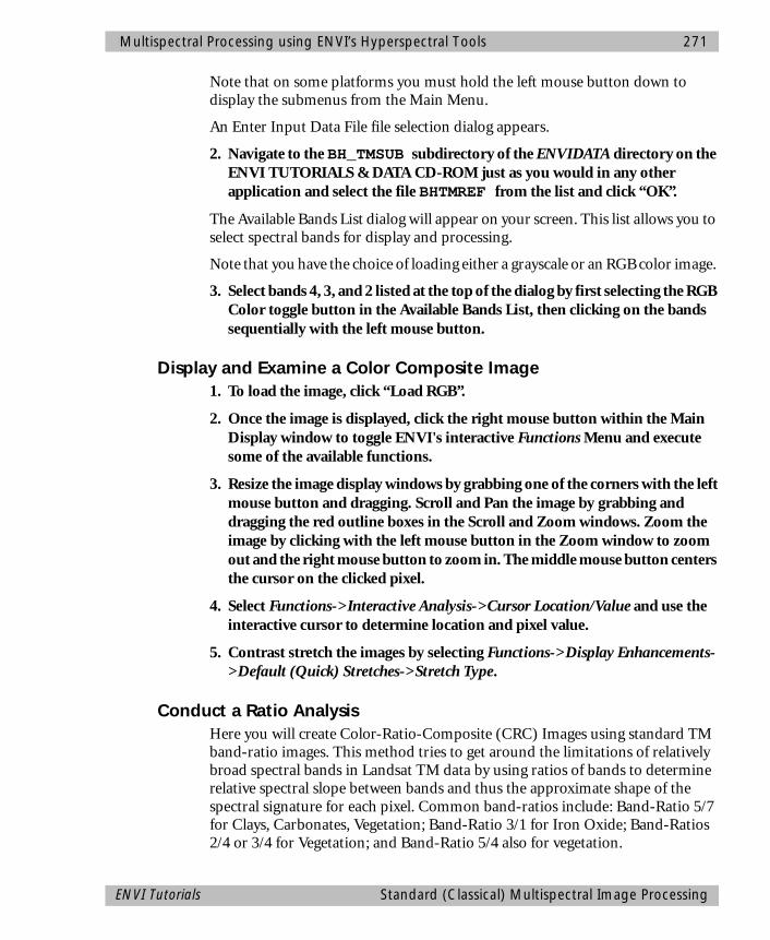
Multispectral Processing using ENVI’s Hyperspectral Tools 271
Note that on some platforms you must hold the left mouse button down to display the submenus from the Main Menu.
An Enter Input Data File file selection dialog appears.
2. Navigate to the BH_TMSUB subdirectory of the ENVIDATA directory on the ENVI TUTORIALS & DATA CD-ROM just as you would in any other application and select the file BHTMREF from the list and click “OK”.
The Available Bands List dialog will appear on your screen. This list allows you to select spectral bands for display and processing.
Note that you have the choice of loading either a grayscale or an RGB color image.
3. Select bands 4, 3, and 2 listed at the top of the dialog by first selecting the RGB Color toggle button in the Available Bands List, then clicking on the bands sequentially with the left mouse button.
Display and Examine a Color Composite Image1. To load the image, click “Load RGB”.
2. Once the image is displayed, click the right mouse button within the Main Display window to toggle ENVI's interactive Functions Menu and execute some of the available functions.
3. Resize the image display windows by grabbing one of the corners with the left mouse button and dragging. Scroll and Pan the image by grabbing and dragging the red outline boxes in the Scroll and Zoom windows. Zoom the image by clicking with the left mouse button in the Zoom window to zoom out and the right mouse button to zoom in. The middle mouse button centers the cursor on the clicked pixel.
4. Select Functions->Interactive Analysis->Cursor Location/Value and use the interactive cursor to determine location and pixel value.
5. Contrast stretch the images by selecting Functions->Display Enhancements->Default (Quick) Stretches->Stretch Type.
Conduct a Ratio AnalysisHere you will create Color-Ratio-Composite (CRC) Images using standard TM band-ratio images. This method tries to get around the limitations of relatively broad spectral bands in Landsat TM data by using ratios of bands to determine relative spectral slope between bands and thus the approximate shape of the spectral signature for each pixel. Common band-ratios include: Band-Ratio 5/7 for Clays, Carbonates, Vegetation; Band-Ratio 3/1 for Iron Oxide; Band-Ratios 2/4 or 3/4 for Vegetation; and Band-Ratio 5/4 also for vegetation.
ENVI Tutorials Standard (Classical) Multispectral Image Processing
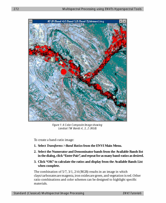
272 Multispectral Processing using ENVI’s Hyperspectral Tools
To create a band-ratio image:
1. Select Transforms->Band Ratios from the ENVI Main Menu.
2. Select the Numerator and Denominator bands from the Available Bands list in the dialog, click “Enter Pair”, and repeat for as many band-ratios as desired.
3. Click “OK” to calculate the ratios and display from the Available Bands List when complete.
The combination of 5/7, 3/1, 2/4 (RGB) results in an image in which clays/carbonates are magenta, iron oxides are green, and vegetation is red. Other ratio combinations and color schemes can be designed to highlight specific materials.
Figure 1: A Color Composite Image showing Landsat TM Bands 4, 3, 2 (RGB)
Standard (Classical) Multispectral Image Processing ENVI Tutorials
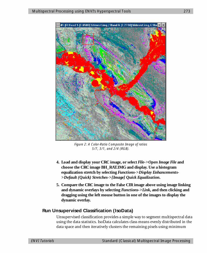
Multispectral Processing using ENVI’s Hyperspectral Tools 273
4. Load and display your CRC image, or select File->Open Image File and choose the CRC image BH_RAT.IMG and display. Use a histogram equalization stretch by selecting Functions->Display Enhancements->Default (Quick) Stretches->[Image] Quick Equalization.
5. Compare the CRC image to the False CIR image above using image linking and dynamic overlays by selecting Functions->Link, and then clicking and dragging using the left mouse button in one of the images to display the dynamic overlay.
Run Unsupervised Classification (IsoData)Unsupervised classification provides a simple way to segment multispectral data using the data statistics. IsoData calculates class means evenly distributed in the data space and then iteratively clusters the remaining pixels using minimum
Figure 2: A Color-Ratio Composite Image of ratios 5/7, 3/1, and 2/4 (RGB).
ENVI Tutorials Standard (Classical) Multispectral Image Processing
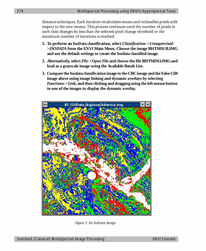
274 Multispectral Processing using ENVI’s Hyperspectral Tools
distance techniques. Each iteration recalculates means and reclassifies pixels with respect to the new means. This process continues until the number of pixels in each class changes by less than the selected pixel change threshold or the maximum number of iterations is reached.
1. To perform an IsoData classification, select Classification->Unsupervised->ISODATA from the ENVI Main Menu. Choose the image BHTMSUB.IMG and use the default settings to create the Isodata classified image.
2. Alternatively, select File->Open File and choose the file BHTMISO.IMG and load as a grayscale image using the Available Bands List.
3. Compare the Isodata classification image to the CRC image and the False CIR image above using image linking and dynamic overlays by selecting Functions->Link, and then clicking and dragging using the left mouse button in one of the images to display the dynamic overlay.
Figure 3: An IsoData Image.
Standard (Classical) Multispectral Image Processing ENVI Tutorials
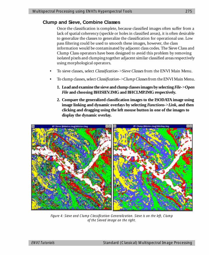
Multispectral Processing using ENVI’s Hyperspectral Tools 275
Clump and Sieve, Combine ClassesOnce the classification is complete, because classified images often suffer from a lack of spatial coherency (speckle or holes in classified areas), it is often desirable to generalize the classes to generalize the classification for operational use. Low pass filtering could be used to smooth these images, however, the class information would be contaminated by adjacent class codes. The Sieve Class and Clump Class operators have been designed to avoid this problem by removing isolated pixels and clumping together adjacent similar classified areas respectively using morphological operators.
• To sieve classes, select Classification->Sieve Classes from the ENVI Main Menu.
• To clump classes, select Classification->Clump Classes from the ENVI Main Menu.
1. Load and examine the sieve and clump classes images by selecting File->Open File and choosing BHISIEV.IMG and BHCLMP.IMG respectively.
2. Compare the generalized classification images to the ISODATA image using image linking and dynamic overlays by selecting Functions->Link, and then clicking and dragging using the left mouse button in one of the images to display the dynamic overlay.
Figure 4: Sieve and Clump Classification Generalization. Sieve is on the left, Clump of the Sieved image on the right.
ENVI Tutorials Standard (Classical) Multispectral Image Processing
276 Multispectral Processing using ENVI’s Hyperspectral Tools
Annotate and Output MapThe final output from any image processing within ENVI is usually a map-oriented, scaled image-map for presentation or visual analysis and interpretation. In this case, the TM data were already geographically referenced, however, ENVI includes full image-to-image and image-to-map registration capabilities. Please see the Registration Tutorial or the ENVI User’s Guide and on-line tutorials.
ENVI also provides all of the tools to produce fully annotated publication-quality maps. This includes pixel, map, and geographic (latitude/longitude) grids; scale-bars; declination diagrams and north arrows; text and symbols; polygons, polylines, and geometric shapes (circles, rectangles); map keys and legends; and image insets. For additional information on map composition, please see the Map Composition Tutorial or the ENVI User’s Guide and on-line tutorials.
1. To add a grid to the displayed Isodata classification, select Functions->Overlays->Grid Lines. Choose File->Restore Setup, click on the file BHTM.GRD and Open. To add the grid to the image, click Apply in the Grid Line Parameters dialog.
2. To add map annotation to the displayed Isodata classification, select Functions->Overlays->Annotation. Choose File->Restore Annotation and pick the file BHTMISO.ANN and click on Open. The map annotation will be loaded onto the image.
Application of ENVI’S Hyperspectral Tools to Multispectral Data Analysis
Read TM Tape or CDAs described above, ENVI provides the tools to read standard Landsat Thematic Mapper data from both tape and CD/disk.
• To read from tape, select Utilities->Tape Utilities->Read Known Tape Formats->Landsat TM (or NLAPS for new EDC-format tapes) from the ENVI Main Menu.
• To read from disk, either select File->Open File->FAST or for NLAPS data select File->Remote Sensing Formats->NLAPS CD.
• For the purposes of this exercise, the data have already been read in and subsetted and the file BH_TMREF.IMG is provided for analysis. This image has been corrected to reflectance using ENVI’s TM Calibration Utility, accessed using Utilities->Data Specific Utilities->Landsat TM->Landsat TM Calibration (See Below)
Application of ENVI’S Hyperspectral Tools to Multispectral Data Analysis ENVI Tutorials
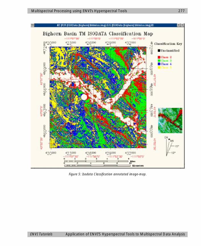
Multispectral Processing using ENVI’s Hyperspectral Tools 277
Figure 5: Isodata Classification annotated image-map.
ENVI Tutorials Application of ENVI’S Hyperspectral Tools to Multispectral Data Analysis
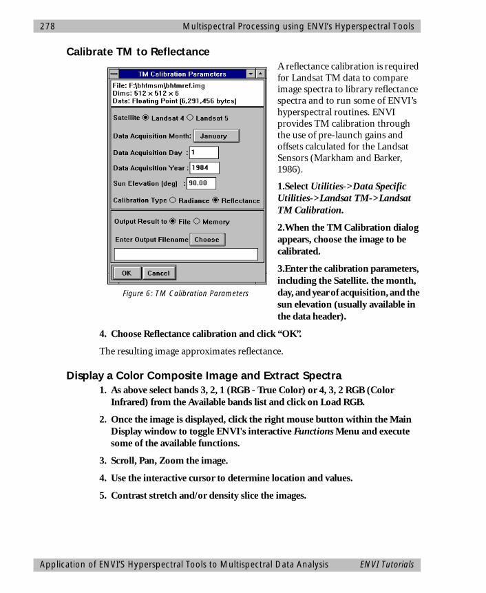
278 Multispectral Processing using ENVI’s Hyperspectral Tools
Calibrate TM to ReflectanceA reflectance calibration is required for Landsat TM data to compare image spectra to library reflectance spectra and to run some of ENVI’s hyperspectral routines. ENVI provides TM calibration through the use of pre-launch gains and offsets calculated for the Landsat Sensors (Markham and Barker, 1986).
1.Select Utilities->Data Specific Utilities->Landsat TM->Landsat TM Calibration.
2.When the TM Calibration dialog appears, choose the image to be calibrated.
3.Enter the calibration parameters, including the Satellite. the month, day, and year of acquisition, and the sun elevation (usually available in the data header).
4. Choose Reflectance calibration and click “OK”.
The resulting image approximates reflectance.
Display a Color Composite Image and Extract Spectra1. As above select bands 3, 2, 1 (RGB - True Color) or 4, 3, 2 RGB (Color
Infrared) from the Available bands list and click on Load RGB.
2. Once the image is displayed, click the right mouse button within the Main Display window to toggle ENVI's interactive Functions Menu and execute some of the available functions.
3. Scroll, Pan, Zoom the image.
4. Use the interactive cursor to determine location and values.
5. Contrast stretch and/or density slice the images.
Figure 6: TM Calibration Parameters
Application of ENVI’S Hyperspectral Tools to Multispectral Data Analysis ENVI Tutorials

Multispectral Processing using ENVI’s Hyperspectral Tools 279
6. Extract Z-profiles (reflectance spectra) from the data by selecting Functions->Profiles->Z Profile in the Main Display window and browse around the image by clicking and dragging the red Zoom Window box using the left mouse button.
Run Minimum Noise Fraction (MNF) TransformationMNF Transform is a method similar to Principal Components used to segregate noise in the data, determine inherent data dimensionality, and reduce computational requirements for subsequent processing (Green et al., 1988; Boardman and Kruse, 1994). For hyperspectral data (less-so for multispectral
Figure 7: Landsat TM reflectance spectra.
ENVI Tutorials Application of ENVI’S Hyperspectral Tools to Multispectral Data Analysis
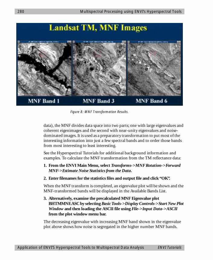
280 Multispectral Processing using ENVI’s Hyperspectral Tools
data), the MNF divides data space into two parts; one with large eigenvalues and coherent eigenimages and the second with near-unity eigenvalues and noise-dominated images. It is used as a preparatory transformation to put most of the interesting information into just a few spectral bands and to order those bands from most interesting to least interesting.
See the Hyperspectral Tutorials for additional background information and examples. To calculate the MNF transformation from the TM reflectance data:
1. From the ENVI Main Menu, select Transforms->MNF Rotation->Forward MNF->Estimate Noise Statistics from the Data.
2. Enter filenames for the statistics files and output file and click “OK”.
When the MNF transform is completed, an eigenvalue plot will be shown and the MNF-transformed bands will be displayed in the Available Bands List.
3. Alternatively, examine the precalculated MNF Eigenvalue plot BHTMMNF.ASC by selecting Basic Tools->Display Controls->Start New Plot Window and then loading the ASCII file using File->Input Data->ASCII from the plot window menu bar.
The decreasing eigenvalue with increasing MNF band shown in the eigenvalue plot above shows how noise is segregated in the higher number MNF bands.
Figure 8: MNF Transformation Results.
Application of ENVI’S Hyperspectral Tools to Multispectral Data Analysis ENVI Tutorials
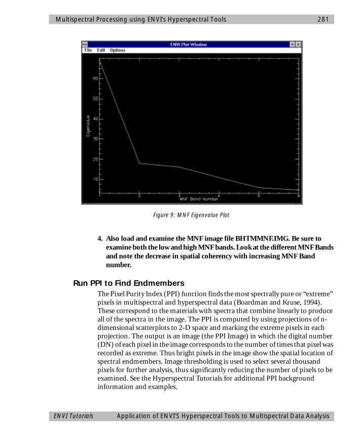
Multispectral Processing using ENVI’s Hyperspectral Tools 281
4. Also load and examine the MNF image file BHTMMNF.IMG. Be sure to examine both the low and high MNF bands. Look at the different MNF Bands and note the decrease in spatial coherency with increasing MNF Band number.
Run PPI to Find EndmembersThe Pixel Purity Index (PPI) function finds the most spectrally pure or “extreme” pixels in multispectral and hyperspectral data (Boardman and Kruse, 1994). These correspond to the materials with spectra that combine linearly to produce all of the spectra in the image. The PPI is computed by using projections of n-dimensional scatterplots to 2-D space and marking the extreme pixels in each projection. The output is an image (the PPI Image) in which the digital number (DN) of each pixel in the image corresponds to the number of times that pixel was recorded as extreme. Thus bright pixels in the image show the spatial location of spectral endmembers. Image thresholding is used to select several thousand pixels for further analysis, thus significantly reducing the number of pixels to be examined. See the Hyperspectral Tutorials for additional PPI background information and examples.
Figure 9: MNF Eigenvalue Plot
ENVI Tutorials Application of ENVI’S Hyperspectral Tools to Multispectral Data Analysis
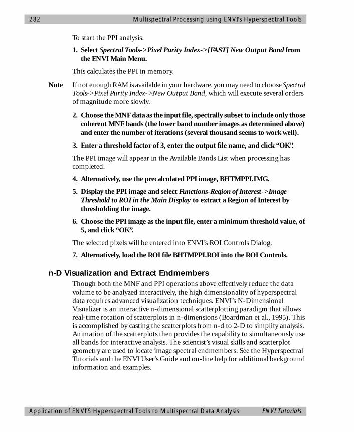
282 Multispectral Processing using ENVI’s Hyperspectral Tools
To start the PPI analysis:
1. Select Spectral Tools->Pixel Purity Index->[FAST] New Output Band from the ENVI Main Menu.
This calculates the PPI in memory.
Note If not enough RAM is available in your hardware, you may need to choose Spectral Tools->Pixel Purity Index->New Output Band, which will execute several orders of magnitude more slowly.
2. Choose the MNF data as the input file, spectrally subset to include only those coherent MNF bands (the lower band number images as determined above) and enter the number of iterations (several thousand seems to work well).
3. Enter a threshold factor of 3, enter the output file name, and click “OK”.
The PPI image will appear in the Available Bands List when processing has completed.
4. Alternatively, use the precalculated PPI image, BHTMPPI.IMG.
5. Display the PPI image and select Functions-Region of Interest->Image Threshold to ROI in the Main Display to extract a Region of Interest by thresholding the image.
6. Choose the PPI image as the input file, enter a minimum threshold value, of 5, and click “OK”.
The selected pixels will be entered into ENVI’s ROI Controls Dialog.
7. Alternatively, load the ROI file BHTMPPI.ROI into the ROI Controls.
n-D Visualization and Extract EndmembersThough both the MNF and PPI operations above effectively reduce the data volume to be analyzed interactively, the high dimensionality of hyperspectral data requires advanced visualization techniques. ENVI’s N-Dimensional Visualizer is an interactive n-dimensional scatterplotting paradigm that allows real-time rotation of scatterplots in n-dimensions (Boardman et al., 1995). This is accomplished by casting the scatterplots from n-d to 2-D to simplify analysis. Animation of the scatterplots then provides the capability to simultaneously use all bands for interactive analysis. The scientist’s visual skills and scatterplot geometry are used to locate image spectral endmembers. See the Hyperspectral Tutorials and the ENVI User’s Guide and on-line help for additional background information and examples.
Application of ENVI’S Hyperspectral Tools to Multispectral Data Analysis ENVI Tutorials
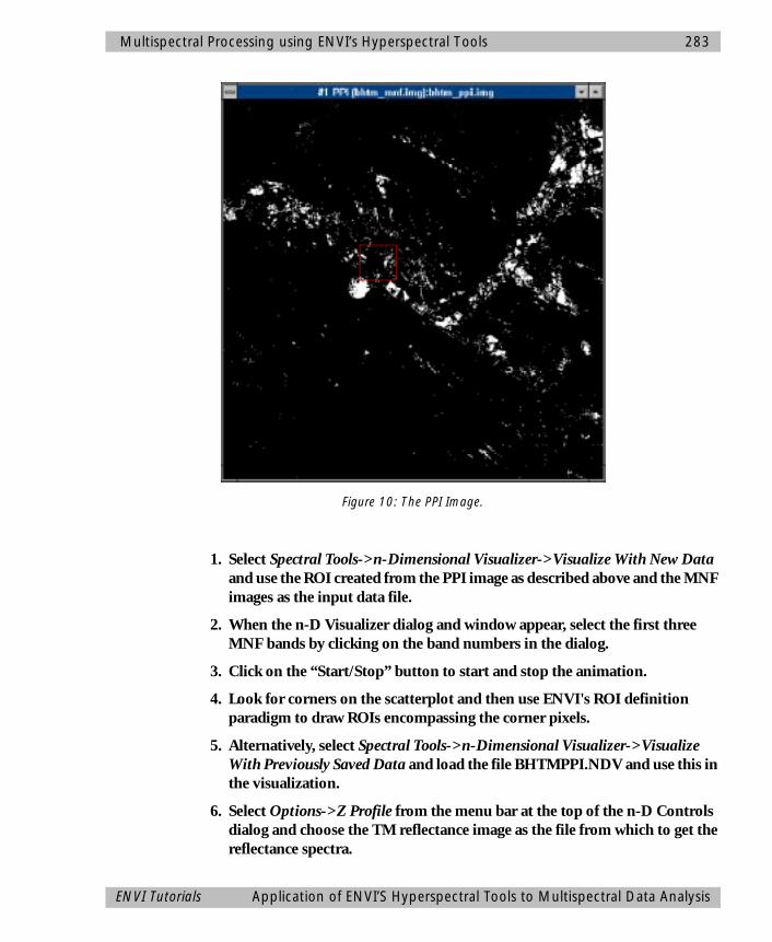
Multispectral Processing using ENVI’s Hyperspectral Tools 283
1. Select Spectral Tools->n-Dimensional Visualizer->Visualize With New Data and use the ROI created from the PPI image as described above and the MNF images as the input data file.
2. When the n-D Visualizer dialog and window appear, select the first three MNF bands by clicking on the band numbers in the dialog.
3. Click on the “Start/Stop” button to start and stop the animation.
4. Look for corners on the scatterplot and then use ENVI's ROI definition paradigm to draw ROIs encompassing the corner pixels.
5. Alternatively, select Spectral Tools->n-Dimensional Visualizer->Visualize With Previously Saved Data and load the file BHTMPPI.NDV and use this in the visualization.
6. Select Options->Z Profile from the menu bar at the top of the n-D Controls dialog and choose the TM reflectance image as the file from which to get the reflectance spectra.
Figure 10: The PPI Image.
ENVI Tutorials Application of ENVI’S Hyperspectral Tools to Multispectral Data Analysis
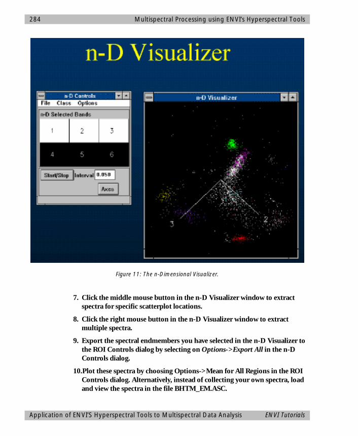
284 Multispectral Processing using ENVI’s Hyperspectral Tools
7. Click the middle mouse button in the n-D Visualizer window to extract spectra for specific scatterplot locations.
8. Click the right mouse button in the n-D Visualizer window to extract multiple spectra.
9. Export the spectral endmembers you have selected in the n-D Visualizer to the ROI Controls dialog by selecting on Options->Export All in the n-D Controls dialog.
10.Plot these spectra by choosing Options->Mean for All Regions in the ROI Controls dialog. Alternatively, instead of collecting your own spectra, load and view the spectra in the file BHTM_EM.ASC.
Figure 11: The n-Dimensional Visualizer.
Application of ENVI’S Hyperspectral Tools to Multispectral Data Analysis ENVI Tutorials
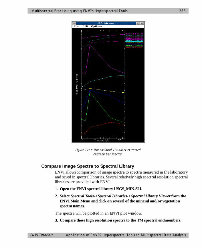
Multispectral Processing using ENVI’s Hyperspectral Tools 285
Compare Image Spectra to Spectral LibraryENVI allows comparison of image spectra to spectra measured in the laboratory and saved in spectral libraries. Several relatively high spectral resolution spectral libraries are provided with ENVI.
1. Open the ENVI spectral library USGS_MIN.SLI.
2. Select Spectral Tools->Spectral Libraries->Spectral Library Viewer from the ENVI Main Menu and click on several of the mineral and/or vegetation spectra names.
The spectra will be plotted in an ENVI plot window.
3. Compare these high resolution spectra to the TM spectral endmembers.
Figure 12: n-Dimensional Visualizer-extracted endmember spectra.
ENVI Tutorials Application of ENVI’S Hyperspectral Tools to Multispectral Data Analysis
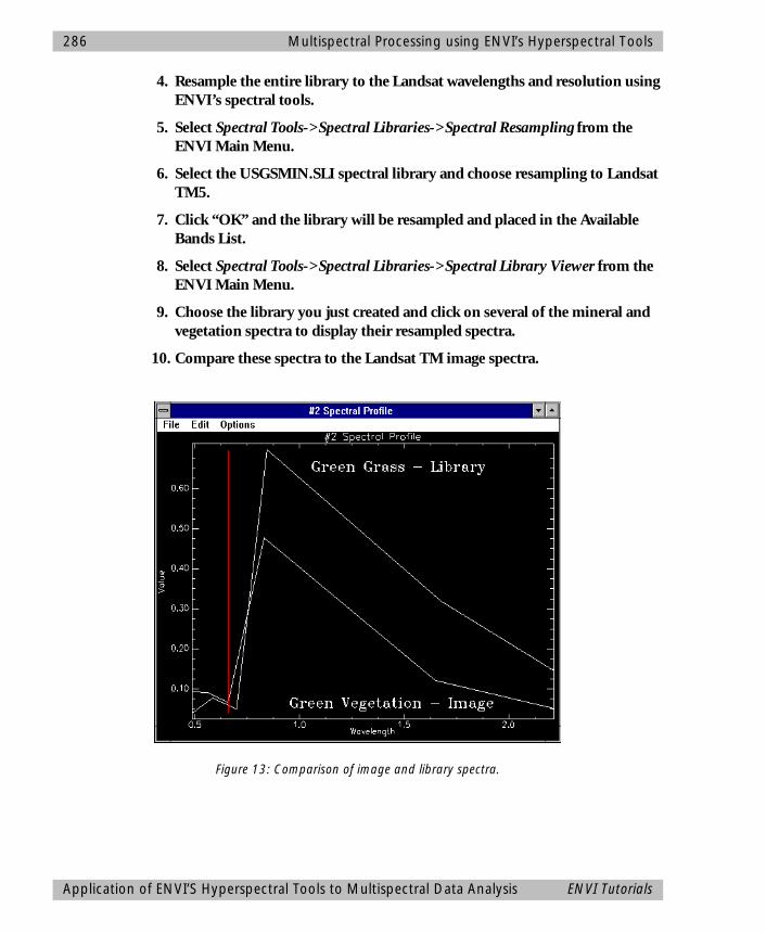
286 Multispectral Processing using ENVI’s Hyperspectral Tools
4. Resample the entire library to the Landsat wavelengths and resolution using ENVI’s spectral tools.
5. Select Spectral Tools->Spectral Libraries->Spectral Resampling from the ENVI Main Menu.
6. Select the USGSMIN.SLI spectral library and choose resampling to Landsat TM5.
7. Click “OK” and the library will be resampled and placed in the Available Bands List.
8. Select Spectral Tools->Spectral Libraries->Spectral Library Viewer from the ENVI Main Menu.
9. Choose the library you just created and click on several of the mineral and vegetation spectra to display their resampled spectra.
10. Compare these spectra to the Landsat TM image spectra.
Figure 13: Comparison of image and library spectra.
Application of ENVI’S Hyperspectral Tools to Multispectral Data Analysis ENVI Tutorials
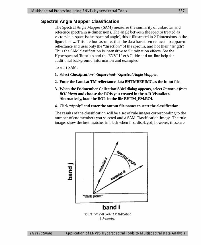
Multispectral Processing using ENVI’s Hyperspectral Tools 287
Spectral Angle Mapper ClassificationThe Spectral Angle Mapper (SAM) measures the similarity of unknown and reference spectra in n-dimensions. The angle between the spectra treated as vectors in n-space is the “spectral angle”, this is illustrated in 2 Dimensions in the figure below. This method assumes that the data have been reduced to apparent reflectance and uses only the “direction” of the spectra, and not their “length”. Thus the SAM classification is insensitive to illumination effects. See the Hyperspectral Tutorials and the ENVI User’s Guide and on-line help for additional background information and examples.
To start SAM:
1. Select Classification->Supervised->Spectral Angle Mapper.
2. Enter the Landsat TM reflectance data BHTMREF.IMG as the input file.
3. When the Endmember Collection:SAM dialog appears, select Import->from ROI Mean and choose the ROIs you created in the n-D Visualizer. Alternatively, load the ROIs in the file BHTM_EM.ROI.
4. Click “Apply” and enter the output file names to start the classification.
The results of the classification will be a set of rule images corresponding to the number of endmembers you selected and a SAM Classification Image. The rule images show the best matches in black when first displayed, however, these are
Figure 14: 2-D SAM Classification Schematic.
ENVI Tutorials Application of ENVI’S Hyperspectral Tools to Multispectral Data Analysis
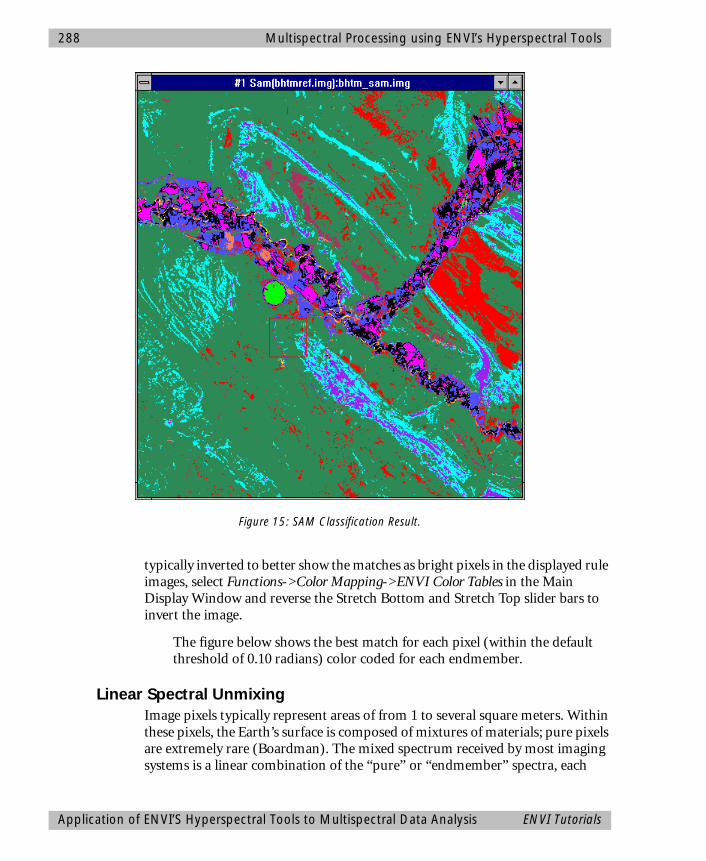
288 Multispectral Processing using ENVI’s Hyperspectral Tools
typically inverted to better show the matches as bright pixels in the displayed rule images, select Functions->Color Mapping->ENVI Color Tables in the Main Display Window and reverse the Stretch Bottom and Stretch Top slider bars to invert the image.
The figure below shows the best match for each pixel (within the default threshold of 0.10 radians) color coded for each endmember.
Linear Spectral UnmixingImage pixels typically represent areas of from 1 to several square meters. Within these pixels, the Earth’s surface is composed of mixtures of materials; pure pixels are extremely rare (Boardman). The mixed spectrum received by most imaging systems is a linear combination of the “pure” or “endmember” spectra, each
Figure 15: SAM Classification Result.
Application of ENVI’S Hyperspectral Tools to Multispectral Data Analysis ENVI Tutorials
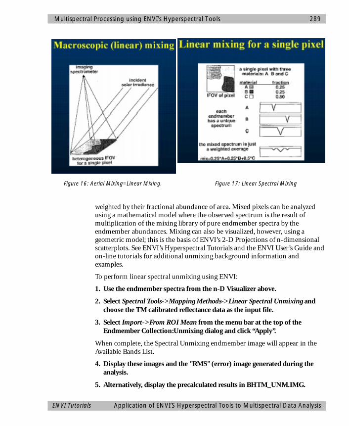
Multispectral Processing using ENVI’s Hyperspectral Tools 289
weighted by their fractional abundance of area. Mixed pixels can be analyzed using a mathematical model where the observed spectrum is the result of multiplication of the mixing library of pure endmember spectra by the endmember abundances. Mixing can also be visualized, however, using a geometric model; this is the basis of ENVI’s 2-D Projections of n-dimensional scatterplots. See ENVI’s Hyperspectral Tutorials and the ENVI User’s Guide and on-line tutorials for additional unmixing background information and examples.
To perform linear spectral unmixing using ENVI:
1. Use the endmember spectra from the n-D Visualizer above.
2. Select Spectral Tools->Mapping Methods->Linear Spectral Unmixing and choose the TM calibrated reflectance data as the input file.
3. Select Import->From ROI Mean from the menu bar at the top of the Endmember Collection:Unmixing dialog and click “Apply”.
When complete, the Spectral Unmixing endmember image will appear in the Available Bands List.
4. Display these images and the "RMS" (error) image generated during the analysis.
5. Alternatively, display the precalculated results in BHTM_UNM.IMG.
Figure 16: Aerial Mixing=Linear Mixing. Figure 17: Linear Spectral Mixing
E
NVI Tutorials Application of ENVI’S Hype rspectral Tools to Multispectral Data Analysis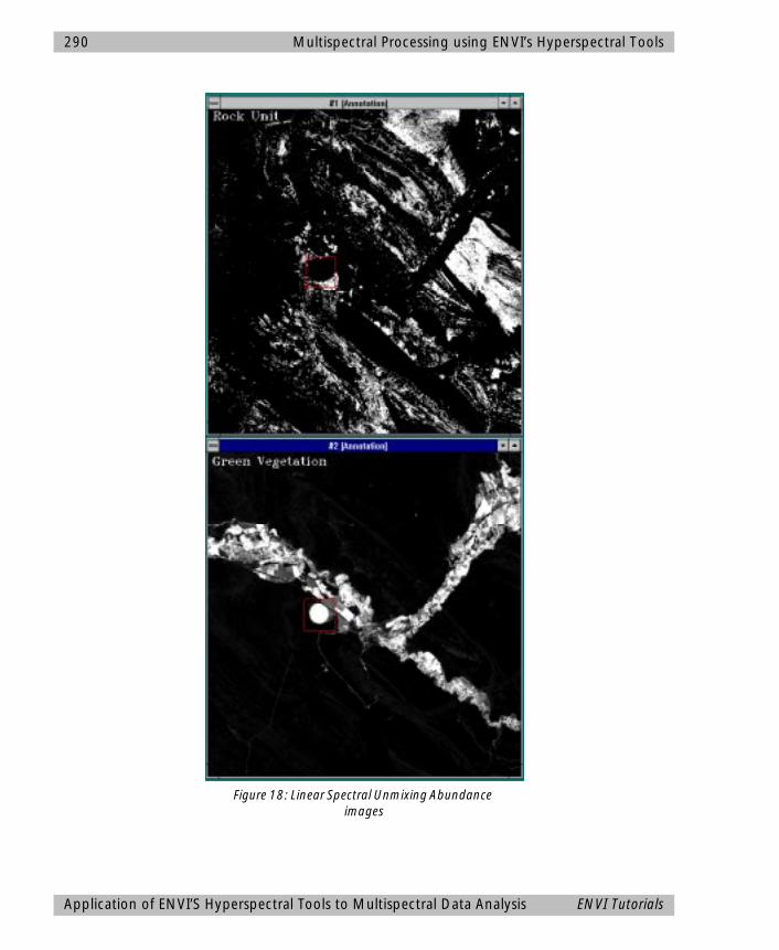
290 Multispectral Processing using ENVI’s Hyperspectral Tools
Figure 18: Linear Spectral Unmixing Abundance images
Application of ENVI’S Hyperspectral Tools to Multispectral Data Analysis ENVI Tutorials
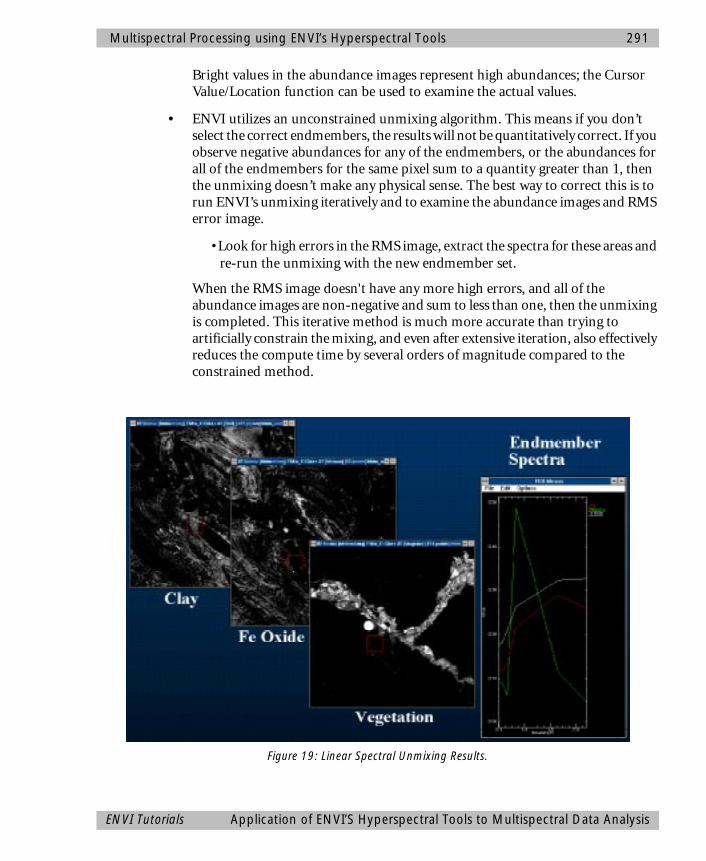
Multispectral Processing using ENVI’s Hyperspectral Tools 291
Bright values in the abundance images represent high abundances; the Cursor Value/Location function can be used to examine the actual values.
• ENVI utilizes an unconstrained unmixing algorithm. This means if you don’t select the correct endmembers, the results will not be quantitatively correct. If you observe negative abundances for any of the endmembers, or the abundances for all of the endmembers for the same pixel sum to a quantity greater than 1, then the unmixing doesn’t make any physical sense. The best way to correct this is to run ENVI’s unmixing iteratively and to examine the abundance images and RMS error image.
• Look for high errors in the RMS image, extract the spectra for these areas and re-run the unmixing with the new endmember set.
When the RMS image doesn't have any more high errors, and all of the abundance images are non-negative and sum to less than one, then the unmixing is completed. This iterative method is much more accurate than trying to artificially constrain the mixing, and even after extensive iteration, also effectively reduces the compute time by several orders of magnitude compared to the constrained method.
Figure 19: Linear Spectral Unmixing Results.
ENVI Tutorials Application of ENVI’S Hyperspectral Tools to Multispectral Data Analysis
292 Multispectral Processing using ENVI’s Hyperspectral Tools
Annotate and Output MapAs previously described, the final output from any image processing within ENVI is usually a map-oriented, scaled image-map for presentation or visual analysis and interpretation. In this case, the TM data were already geographically referenced, however, ENVI includes full image-to-image and image-to-map registration capabilities. Please see the Registration Tutorial in this volume or the ENVI User’s Guide and on-line help. ENVI also provides all of the tools to produce fully annotated publication-quality maps. This includes pixel, map, and geographic (latitude/longitude) grids; scale-bars; declination diagrams and north arrows; text and symbols; polygons, polylines, and geometric shapes (circles, rectangles); map keys and legends; and image insets. For additional information on map composition, please see the Map Composition Tutorial or the ENVI User’s Guide or on-line help.
SummaryA wide variety of advanced tools have been developed for analysis of imaging spectrometer (hyperspectral data). These tools are mature and are being used operationally for analysis of AVIRIS and other datasets. We don't have hyperspectral data for many of the areas we would like to investigate, however, widely available mulispectral data can be analyzed using some of the “hyperspectral” tools. ENVI allows users to use approaches developed for analysis of hyperspectral data to provide new insight to the use and analysis of multispectral datasets.
ReferencesBoardman, J. W., Kruse, F. A., and Green, R. O., 1995, Mapping target signatures via partial unmixing of AVIRIS data: in Summaries, Fifth JPL Airborne Earth Science Workshop, JPL Publication 95-1, v. 1, p. 23-26.
Boardman, J. W., 1993, Automated spectral unmixing of AVIRIS data using convex geometry concepts: in Summaries, Fourth JPL Airborne Geoscience Workshop, JPL Publication 93-26, v. 1, p. 11 - 14.
Green, A. A., Berman, M., Switzer, P, and Craig, M. D., 1988, A transformation for ordering multispectral data in terms of image quality with implications for noise removal: IEEE Transactions on Geoscience and Remote Sensing, v. 26, no. 1, p. 65-74.
Markham, B. L., and Barker, J. L.,1986, Landsat MSS and TM post-calibration dynamic ranges, exoatmopspheric reflectances and at-satellite temperatures: EOSAT Landat Technical Notes, No. 1, August 1996.
Summary ENVI Tutorials

Multispectral Processing using ENVI’s Hyperspectral Tools 293
Research Systems Inc, 1997, ENVI User’s Guide, Chapter 10.
Sabins, F. F. Jr., 1986, Remote Sensing Principles and Interpretation: W. H. Freeman and Company, New York, 449 p.
ENVI Tutorials References

294 Multispectral Processing using ENVI’s Hyperspectral Tools
References ENVI Tutorials
ENVI Tutorial #15
Basic SAR Processing and Analysis
The following topics are covered in this tutorial:
Overview of This Tutorial ......................................................................................296Files Used in this Tutorial .......................................................................................296Background ..........................................................................................................297Single-Band SAR Processing Scenario ....................................................................298Image-Map Output...............................................................................................306Summary ..............................................................................................................307
295
296 Basic SAR Processing and Analysis
Overview of This TutorialThis tutorial is designed to give you a working knowledge of ENVI’s basic tools for processing single-band SAR data (such as RadarSat, ERS-1, JERS-1).
Files Used in this TutorialYou must have the ENVI TUTORIALS & DATA CD-ROM mounted on your system to access the filesused by this tutorial, or copy the files to your disk.
The files used in this tutorial are contained in theRSAT_SUB subdirectory of the ENVIDATA direc-tory on the ENVI TUTORIALS & DATA CD-ROM.
Required FilesThe files listed below are required to run this exer-cise.
LEA_01.001 Radarsat Leader File
BONNRSAT.IMG Radarsat Image Subset
BONNRSAT.HDR ENVI Header for Above
RSI_F1.IMG Frost Filter Result
RSI_F1.HDR ENVI Header for Above
DSLICE.DSR Density Slice level save file
RSI_F2.IMG Laplacian Filter Result
RSI_F2.HDR ENVI Header for Above
RSI_F3.IMG Laplacian Filter result with 0.9 addback
RSI_F3.HDR ENVI Header for Above
RSI_FUS.IMG Simulated Fused TM and Radarsat
RSI_FUS.HDR ENVI Header for Above
RSI_MAP.JPG Radarsat map composition example
Topics Covered in This Tutorial
Overview of This Tutorial
Files Used In this Tutorial
Background• Concepts for processing SAR
with ENVI• RadarSat Data
Single-Band SAR Processing Scenario• Read Data from Tape/CD and
Display Images• Review CEOS Header• Contrast Stretching (Square
Root)• Remove Speckle using Adaptive
Filters• Compare Images using
Dynamic Overlay• Density Slice• Edge Enhancement• Data Fusion
Image-Map Output
Summary
Overview of This Tutorial ENVI Tutorials
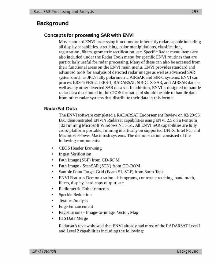
Basic SAR Processing and Analysis 297
Background
Concepts for processing SAR with ENVIMost standard ENVI processing functions are inherently radar capable including all display capabilities, stretching, color manipulations, classification, registration, filters, geometric rectification, etc. Specific Radar menu items are also included under the Radar Tools menu for specific ENVI routines that are particularly useful for radar processing. Many of these can also be accessed from their functional areas on the ENVI main menu. ENVI provides standard and advanced tools for analysis of detected radar images as well as advanced SAR systems such as JPL’s fully polarimetric AIRSAR and SIR-C systems. ENVI can process ERS-1/ERS-2, JERS-1, RADARSAT, SIR-C, X-SAR, and AIRSAR data as well as any other detected SAR data set. In addition, ENVI is designed to handle radar data distributed in the CEOS format, and should be able to handle data from other radar systems that distribute their data in this format.
RadarSat DataThe ENVI software completed a RADARSAT Endorsement Review on 02/29/95. BSC demonstrated ENVI’s Radarsat capabilities using ENVI 2.5 on a Pentium 133 running Microsoft Windows NT 3.51. All ENVI SAR capabilities are fully cross-platform portable, running identically on supported UNIX, Intel PC, and Macintosh/Power Macintosh systems. The demonstration consisted of the following components:
• CEOS Header Browsing
• Ingest Verification
• Path Image (SGF) from CD-ROM
• Path Image - ScanSAR (SCN) from CD-ROM
• Sample Point Target Grid (Beam 51, SGF) from 8mm Tape
• ENVI Features Demonstration - histograms, contrast stretching, band math, filters, display, hard copy output, etc
• Radiometric Enhancements• Speckle Reduction
• Texture Analysis
• Edge Enhancement
• Registrations - Image-to-image, Vector, Map
• IHS Data Merge
Radarsat’s review showed that ENVI already had most of the RADARSAT Level 1 and Level 2 capabilities including the following:
ENVI Tutorials Background
298 Basic SAR Processing and Analysis
Level 1 • Existing features are all radar capable
• Specific required features are already available in ENVI 2.0 at no extra cost • Speckle reduction filters - Lee, Local Sigma, Bit Errors
• Texture Analysis - Data Range, First Moment, Second Moment, RMS
• Edge Enhancements - high pass, laplacian, directional
• Radiometric enhancements - linear, piecewise linear, gaussian, arbitrary, LUTs
• Handling of 16 bit data files
Level 2 • Image-to-Image registration
• Image-to-Vector registration
• Image-to- Map registration
• Mosaicking
• RGB to HIS conversion and data merging•
Radarsat-Specific Routines added to ENVI 2.5ENVI RADARSAT-specific ingest routines and other modifications were added for ENVI version 2.5 including:
• RADARSAT CEOS Reader for CD-ROM, Disk, and Tape with 16 bit or 8 bit ingest
• Compression on ingest
• RADARSAT CEOS Header/Trailer Browser • Support for the following Platforms: UNIX (SUN, SGI, HP, IBM, DEC)
Intel PC (Windows 3.1, Windows NT, Windows 95), MacIntosh and Power MacIntosh
ENVI Version 2.5 was certified as Radarsat Compatible on 02/29/95 and SAR support has subsequently been improved with every version upgrade.
Single-Band SAR Processing ScenarioThis section of the tutorial describes a typical single-band SAR processing scenario from data input through processing and analysis, to publication-quality and/or map output. Data used for the example are a subset of a Radarsat 1 Path Image, Fine Beam 2, December 17, 1995, Bonn, Germany.
Single-Band SAR Processing Scenario ENVI Tutorials
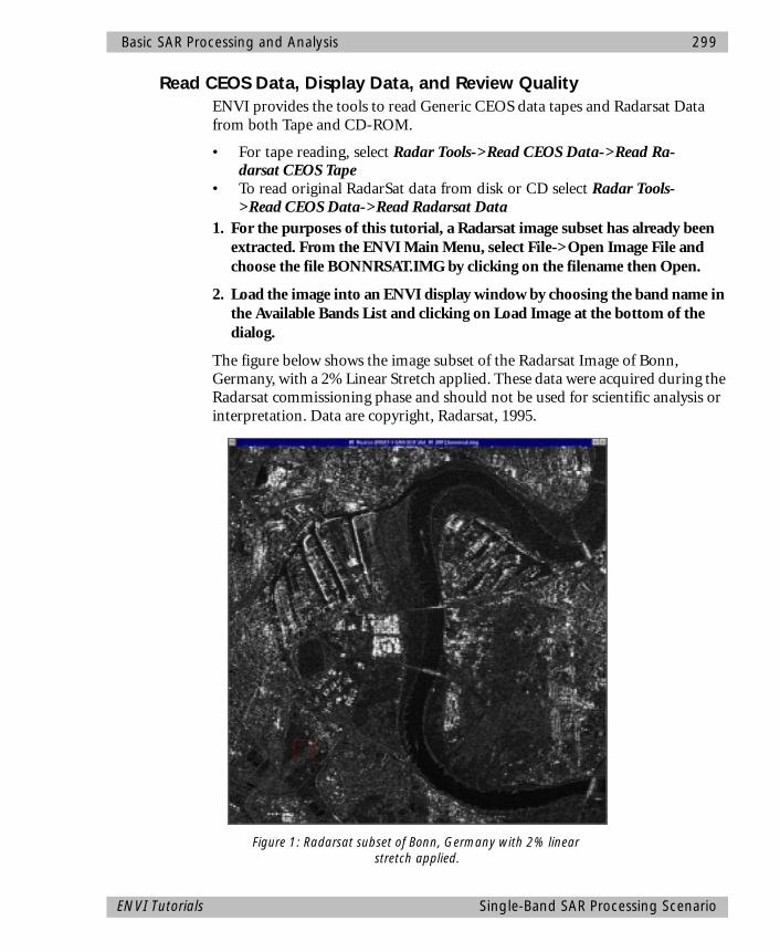
Basic SAR Processing and Analysis 299
Read CEOS Data, Display Data, and Review QualityENVI provides the tools to read Generic CEOS data tapes and Radarsat Data from both Tape and CD-ROM.
• For tape reading, select Radar Tools->Read CEOS Data->Read Ra-darsat CEOS Tape
• To read original RadarSat data from disk or CD select Radar Tools->Read CEOS Data->Read Radarsat Data
1. For the purposes of this tutorial, a Radarsat image subset has already been extracted. From the ENVI Main Menu, select File->Open Image File and choose the file BONNRSAT.IMG by clicking on the filename then Open.
2. Load the image into an ENVI display window by choosing the band name in the Available Bands List and clicking on Load Image at the bottom of the dialog.
The figure below shows the image subset of the Radarsat Image of Bonn, Germany, with a 2% Linear Stretch applied. These data were acquired during the Radarsat commissioning phase and should not be used for scientific analysis or interpretation. Data are copyright, Radarsat, 1995.
Figure 1: Radarsat subset of Bonn, Germany with 2% linear stretch applied.
ENVI Tutorials Single-Band SAR Processing Scenario
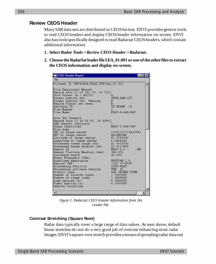
300 Basic SAR Processing and Analysis
Review CEOS HeaderMany SAR data sets are distributed in CEOS format. ENVI provides generic tools to read CEOS headers and display CEOS header information on-screen. ENVI also has tools specifically designed to read Radarsat CEOS headers, which contain additional information.
1. Select Radar Tools->Review CEOS Header->Radarsat.
2. Choose the RadarSat leader file LEA_01.001 or one of the other files to extract the CEOS information and display on-screen.
Contrast Stretching (Square Root)Radar data typically cover a large range of data values. As seen above, default linear stretches do not do a very good job of contrast enhancing most radar images. ENVI’s square-root stretch provides a means of spreading radar data out
Figure 2: Radarsat CEOS Header information from the Leader File.
Single-Band SAR Processing Scenario ENVI Tutorials
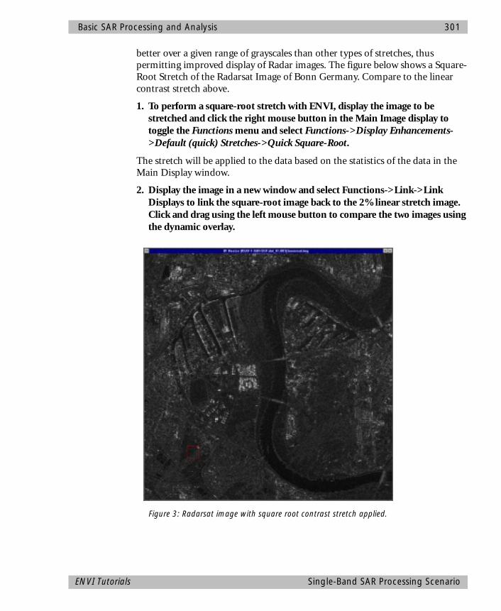
Basic SAR Processing and Analysis 301
better over a given range of grayscales than other types of stretches, thus permitting improved display of Radar images. The figure below shows a Square-Root Stretch of the Radarsat Image of Bonn Germany. Compare to the linear contrast stretch above.
1. To perform a square-root stretch with ENVI, display the image to be stretched and click the right mouse button in the Main Image display to toggle the Functions menu and select Functions->Display Enhancements->Default (quick) Stretches->Quick Square-Root.
The stretch will be applied to the data based on the statistics of the data in the Main Display window.
2. Display the image in a new window and select Functions->Link->Link Displays to link the square-root image back to the 2% linear stretch image. Click and drag using the left mouse button to compare the two images using the dynamic overlay.
Figure 3: Radarsat image with square root contrast stretch applied.
ENVI Tutorials Single-Band SAR Processing Scenario
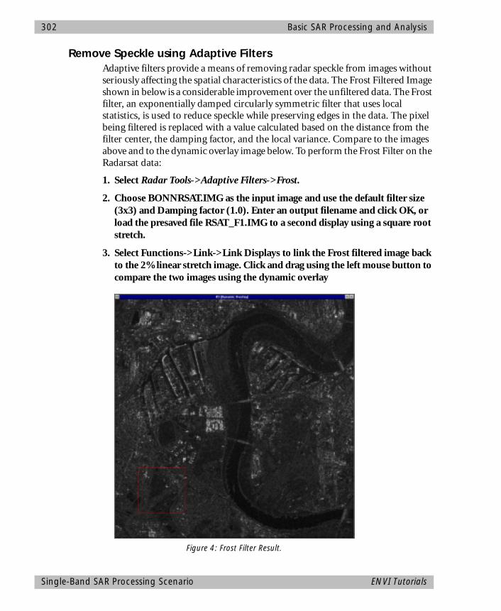
302 Basic SAR Processing and Analysis
Remove Speckle using Adaptive FiltersAdaptive filters provide a means of removing radar speckle from images without seriously affecting the spatial characteristics of the data. The Frost Filtered Image shown in below is a considerable improvement over the unfiltered data. The Frost filter, an exponentially damped circularly symmetric filter that uses local statistics, is used to reduce speckle while preserving edges in the data. The pixel being filtered is replaced with a value calculated based on the distance from the filter center, the damping factor, and the local variance. Compare to the images above and to the dynamic overlay image below. To perform the Frost Filter on the Radarsat data:
1. Select Radar Tools->Adaptive Filters->Frost.
2. Choose BONNRSAT.IMG as the input image and use the default filter size (3x3) and Damping factor (1.0). Enter an output filename and click OK, or load the presaved file RSAT_F1.IMG to a second display using a square root stretch.
3. Select Functions->Link->Link Displays to link the Frost filtered image back to the 2% linear stretch image. Click and drag using the left mouse button to compare the two images using the dynamic overlay
Figure 4: Frost Filter Result.
Single-Band SAR Processing Scenario ENVI Tutorials
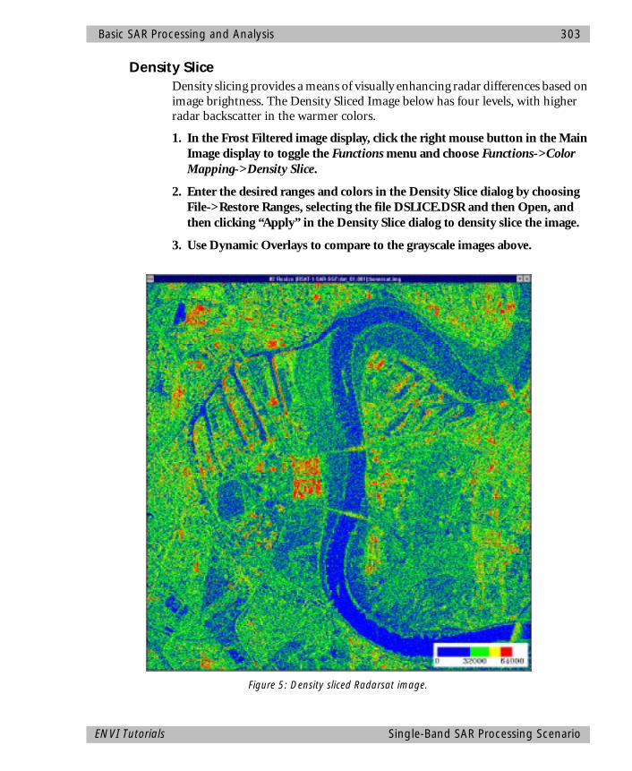
Basic SAR Processing and Analysis 303
Density SliceDensity slicing provides a means of visually enhancing radar differences based on image brightness. The Density Sliced Image below has four levels, with higher radar backscatter in the warmer colors.
1. In the Frost Filtered image display, click the right mouse button in the Main Image display to toggle the Functions menu and choose Functions->Color Mapping->Density Slice.
2. Enter the desired ranges and colors in the Density Slice dialog by choosing File->Restore Ranges, selecting the file DSLICE.DSR and then Open, and then clicking “Apply” in the Density Slice dialog to density slice the image.
3. Use Dynamic Overlays to compare to the grayscale images above.
Figure 5: Density sliced Radarsat image.
ENVI Tutorials Single-Band SAR Processing Scenario
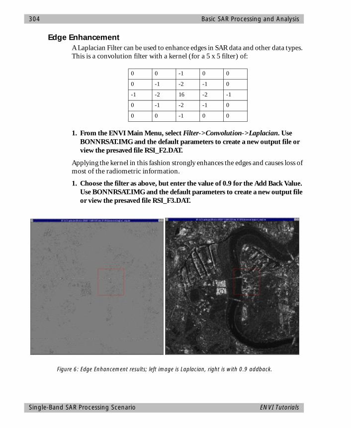
304 Basic SAR Processing and Analysis
Edge EnhancementA Laplacian Filter can be used to enhance edges in SAR data and other data types. This is a convolution filter with a kernel (for a 5 x 5 filter) of:
1. From the ENVI Main Menu, select Filter->Convolution->Laplacian. Use BONNRSAT.IMG and the default parameters to create a new output file or view the presaved file RSI_F2.DAT.
Applying the kernel in this fashion strongly enhances the edges and causes loss of most of the radiometric information.
1. Choose the filter as above, but enter the value of 0.9 for the Add Back Value. Use BONNRSAT.IMG and the default parameters to create a new output file or view the presaved file RSI_F3.DAT.
0 0 -1 0 0
0 -1 -2 -1 0
-1 -2 16 -2 -1
0 -1 -2 -1 0
0 0 -1 0 0
Figure 6: Edge Enhancement results; left image is Laplacian, right is with 0.9 addback.
Single-Band SAR Processing Scenario ENVI Tutorials
Basic SAR Processing and Analysis 305
2. Compare the result to the filtered image and to the original data using dynamic overlays
Data FusionOne of the strengths of SAR data is its highly complementary nature with respect to other data sets. Radar data provides a wealth of spatial information that isn’t present in many other types of image data. Conversely, however, SAR data doesn’t have much compositional information, which is typically expressed in multispectral optical data sets. This situation leads naturally to the use of combined SAR/Optical data.
The most common means of combining data sets is the use of Intensity, Hue, Saturation (IHS) transforms to combine a multispectral, color-composite image with a monochromatic SAR sharpening band. ENVI provides a simple tool to conduct data merging using IHS.
No optical data set was available that corresponded to the Bonn Radarsat data so you are not able to perform this function with these data. The example and figure below, however, illustrate a simulated image showing IHS-Merged Data of an unrelated Landsat Thematic Mapper data set. This image is designed to give you an idea of how a merged SAR/Optical dataset might appear. ENVI also provides a Color Normalization (Brovey) transform for data fusion.
1. Given 3-band color composite image, select Transforms->Image Sharpening-->IHS and then enter the three bands for the color composite into the Select Input RGB Input Bands dialog.
2. Select the single band SAR image.
If the two images have the same spatial dimension, ENVI goes ahead with the fusion. If the two data sets are both georeferenced, but with different pixel sizes, ENVI resamples low resolution image to match the high resolution image, then fuses the two data sets.
ENVI Tutorials Single-Band SAR Processing Scenario
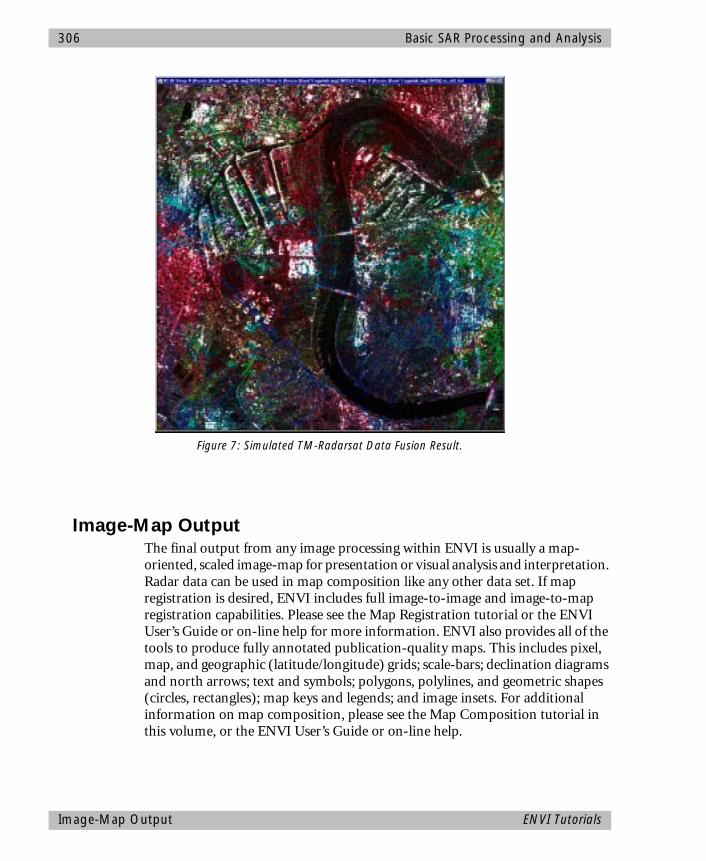
306 Basic SAR Processing and Analysis
Image-Map OutputThe final output from any image processing within ENVI is usually a map-oriented, scaled image-map for presentation or visual analysis and interpretation. Radar data can be used in map composition like any other data set. If map registration is desired, ENVI includes full image-to-image and image-to-map registration capabilities. Please see the Map Registration tutorial or the ENVI User’s Guide or on-line help for more information. ENVI also provides all of the tools to produce fully annotated publication-quality maps. This includes pixel, map, and geographic (latitude/longitude) grids; scale-bars; declination diagrams and north arrows; text and symbols; polygons, polylines, and geometric shapes (circles, rectangles); map keys and legends; and image insets. For additional information on map composition, please see the Map Composition tutorial in this volume, or the ENVI User’s Guide or on-line help.
Figure 7: Simulated TM-Radarsat Data Fusion Result.
Image-Map Output ENVI Tutorials
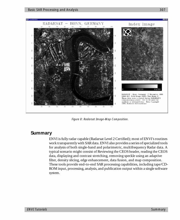
Basic SAR Processing and Analysis 307
SummaryENVI is fully radar capable (Radarsat Level 2 Certified); most of ENVI’s routines work transparently with SAR data. ENVI also provides a series of specialized tools for analysis of both single-band and polarimetric, multifrequency Radar data. A typical scenario might consist of Reviewing the CEOS header, reading the CEOS data, displaying and contrast stretching, removing speckle using an adaptive filter, density slicing, edge enhancement, data fusion, and map composition. These tools provide end-to-end SAR processing capabilities, including tape/CD-ROM input, processing, analysis, and publication output within a single software system.
Figure 8: Radarsat Image-Map Composition.
ENVI Tutorials Summary

308 Basic SAR Processing and Analysis
Summary ENVI Tutorials
ENVI Tutorial #16
Polarimetric SAR Processing and Analysis
The following topics are covered in this tutorial:
Overview of This Tutorial ......................................................................................310Files Used in This Tutorial ......................................................................................310Background: SIR-C/SAR.........................................................................................311Analyzing SIR-C Data ............................................................................................311Synthesize Images - Start The Actual Tutorial Work Here .......................................313Define ROIs for Polarization Signatures..................................................................317Extract Polarization Signatures ..............................................................................319Use Adaptive Filters...............................................................................................321Perform Slant-to-Ground Range Transformation....................................................323Use Texture Analysis..............................................................................................323Create an Image-Map for Output .........................................................................324
309
310 Polarimetric SAR Processing and Analysis
Overview of This TutorialThe following tutorial demonstrates the use of ENVI’s radar data analysis functions. Data from the Spaceborne Imaging Radar-C (SIR-C) for Death Valley, California are used in this example. The data were obtained by SIR-C onboard the Space Shuttle Endeavor in April 1994.
Files Used in This TutorialYou must have the ENVI TUTORIALS & DATA CD-ROM mounted on your system to access the files usedby this tutorial, or copy the files to your disk.
The files used in this tutorial are contained in theNDV_SIRC subdirectory of the ENVIDATA directo-ry on the ENVI TUTORIALS & DATA CD-ROM.
The files listed below are required to run this exercise. Several new files will be generated during the processing steps.
Required FilesNDV_L.CDP L-band SIR-C subset in ENVI Compressed
Data Product .cdp format.
POL_SIG.ROI Saved Regions of Interest (ROI).
TEXTURE.DSR Saved Density Slice Range .dsr file.
Generated FilesNDV_L.SYN Synthesized images (~2.5 Mb, also gener-
ates .hdr file).
NDV_L2.SYN Synthesized images in dB (~5 Mb, also gen-erates .hdr file).
NDV_GAM.IMG Gamma filter result (~0.6 Mb, also gener-ates .hdr file).
NDV_GR.IMG Slant to ground range result (~0.9 Mb, also generates .hdr file).
NDV_HH.TEX Texture filter result (~2.5 Mb, also gen-erates .hdr file).
ENVI.PS Output ENVI postscript file (~3.8 Mb).
Topics Covered in This Tutorial
Background: SIR-C/SAR
Analyzing SIR-C Data• Read a SIR-C CEOS Data Tape• Multilook SIR-C Data• Synthesize Images - Start The
Actual Tutorial Work Here• Display Images• Define ROIs for Polarization
Signatures• Extract Polarization Signatures• Use Adaptive Filters• Perform Slant-to-Ground
Range Transformation• Use Texture Analysis• Output Color-coded Texture
Map
Overview of This Tutorial ENVI Tutorials
Polarimetric SAR Processing and Analysis 311
Background: SIR-C/SARSIR-C is a polarimetric synthetic aperture radar that uses two microwave wavelengths: L-band (24 cm) and C-band (6 cm). The SIR-C radar system was flown as a science experiment on the Space Shuttle Endeavor in April (SRL-1) and October 1994 (SRL-2), collecting high quality SAR data over many sites around the world (a second radar system—“X-SAR”—was also flown on this mission, but these data are not discussed or processed here). Additional information about SIR-C is available on the NASA/JPL Imaging Radar Home Page on the World Wide Web at http://southport.jpl.nasa.gov/.
Analyzing SIR-C DataThe data used in this tutorial are a subset of L-band “Single Look Complex” (SLC) SIR-C data that cover the northern part of Death Valley, including Stovepipe Wells, a site of active sand dunes and extensive alluvial fans at the base of mountains. These data have been pre-processed by reading/subsetting from tape and multilooking (averaging) to 13 m square pixels. The data are provided in a special ENVI “Compressed Data Product (.cdp) format. This is a non-image format similar to the tape format and can not be viewed until images are “synthesized” for specific polarizations.
The first two functions described in this example—reading the data tape and “multilooking”— have been pre-applied to the SIR-C data. We include the sections here for completeness in dealing with SIR-C data. Skip to the section “Synthesize images - Start The Actual Work Here” if you are not interested in reading about data input and preparation.
Read a SIR-C CEOS Data Tape
Note The file used for this exercise has already been read from tape and saved in a file. Instructions on reading a SIR-C tape are included here only for completeness.
1. Select Radar Tools->Read CEOS Data->Read SIR-C CEOS Tape to read a SIR-C CEOS data tape into ENVI.
• Note that this utility can also be accessed by selecting Utilities->Tape Utili-ties->Read Known Tape Formats->SIR-C CEOS
The SIRC Format—Load Tape dialog will appear. See the Tape Reading section of the ENVI User’s Guide for details on the SIR-C tape-reading function. To read a tape:
1. Enter the tape device name and let the record size default to 65,536.
2. Click “OK”.
ENVI Tutorials Background: SIR-C/SAR

312 Polarimetric SAR Processing and Analysis
The tape will be scanned to determine what SIR-C files it contains and a dialog will appear, allowing you to select the desired data sets. By default, ENVI will read all of the data files on the tape.
3. If you do not want to read all of the data files, click “Clear” and then click on the box next to each desired file. When the files are selected, click “OK”.
4. The selected data files can be subset and multilooked independently as they are being read from tape. We recommend, however, that multilooking be performed on disk files unless insufficient disk space is available, as this function is extremely slow from tape.
5. Click on a filename, then click on “Spatial Subset” or “Multi-Look” to enter parameters for the data file and enter an output filename.
Each input file must have an output filename. By convention, the output filenames should take the form filename_c.cdp and filename_l.cdp for the C- and L-bands, respectively.
The SIR-C data will be read from the tape and one compressed scattering matrix output file created for each data set selected.
Multilook SIR-C DataMultilooking is a method for reducing speckle noise in SAR data and for changing the size of a SAR file. SIR-C data can be multilooked to a specified number of looks, number of lines and samples, or azimuth and range resolutions.
Note The SIR-C file used in this tutorial was a single look dataset that had a range resolution of 13 m and an azimuth size of 5 m. Multilooking has already been performed in the azimuth direction to make 13 m square pixel sizes. Instructions on Multilooking are included here only for completeness in dealing with SIR-C data. To multilook a dataset:
1. Select Radar Tools->Polarimetric Tools->Multilook Compressed Data->SIR-C Multilook.
2. When the Input Data Product Files dialog appears, click “Open File” and select the input file.
ENVI will detect whether the file contains L- or C- band data and display the file name in the appropriate field of the dialog.
3. Click “OK”.
4. Select the file to multilook by selecting the box next to the name.
Multiple files can be selected.
Analyzing SIR-C Data ENVI Tutorials
Polarimetric SAR Processing and Analysis 313
5. Enter any one of three values—number of looks, number of pixels, or pixel size—and the other two will be calculated automatically.
Both integer and floating point number of looks are supported.
6. Enter the desired values in the appropriate box for both “Samples (range)” and “Lines (azimuth)”.
7. Enter the base file name in the appropriate text box and click “OK”.
Synthesize Images - Start The Actual Tutorial Work HereThe SIR-C quad-polarization data provided with this tutorial and available on tape from JPL are in a non-image, compressed format. Accordingly, images of the SIR-C data must be mathematically synthesized from the compressed scattering matrix data. You can synthesize images of any transmit and receive polarization combinations desired.
1. Select Radar Tools->Polarimetric Tools->Decompress-Synthesize Images->Synthesize SIR-C Images.
2. When the Input Product Data Files dialog appears, click “Open File” to display a standard file selection dialog and navigate to the NDV_SIRC subdirectory of the ENVIDATA directory.
3. Select the file NDV_L.CDP from the list. When the filename appears in the “Selected Files L:” field, click “OK”.
The Synthesize Parameters dialog appears.
Default Polarization CombinationsFour standard transmit/receive polarization combinations—HH, VV, HV, and TP—will be listed in the “Select Bands to Synthesize” list in the Synthesize Parameters dialog. By default, these bands are selected to be synthesized.
1. Enter the output filename NDV_L.SYN in the “Enter Output Filename” field.
2. Select “Byte” from the “Output Data Type” pulldown menu. This will scale the output data to byte values. Make the appropriate selections and click OK.
Note If you will be doing quantitative analysis, the output should remain in floating point format.
An ENVI Status Window will appear and after a short wait, the file NDV_L.SYN will be created, and four bands corresponding to the four polarization
ENVI Tutorials Synthesize Images - Start The Actual Tutorial Work Here
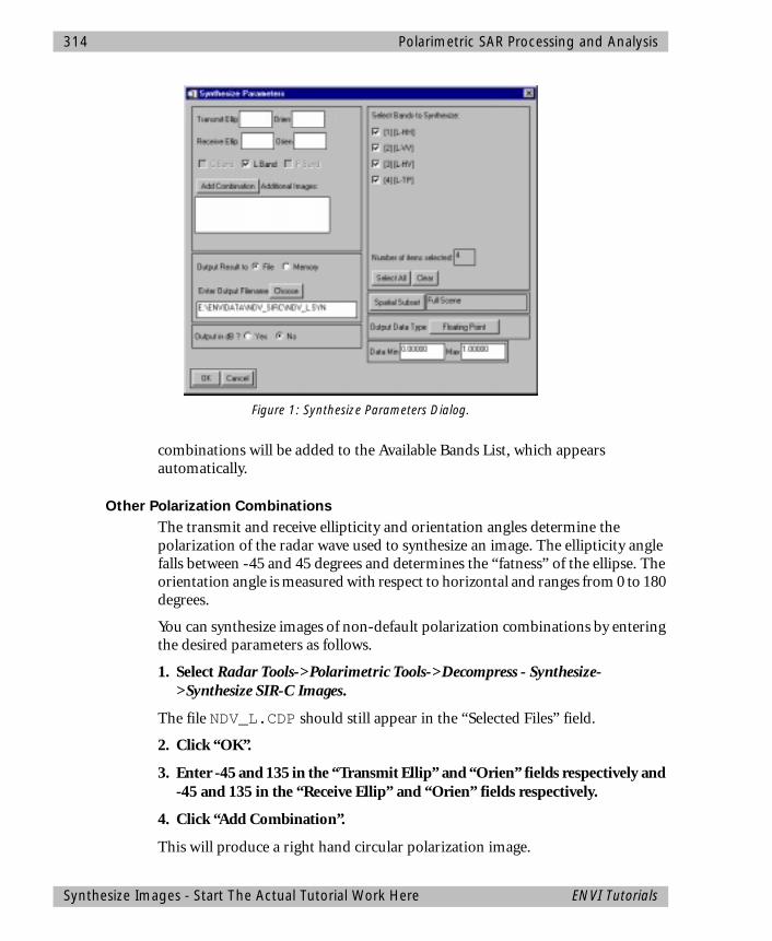
314 Polarimetric SAR Processing and Analysis
combinations will be added to the Available Bands List, which appears automatically.
Other Polarization CombinationsThe transmit and receive ellipticity and orientation angles determine the polarization of the radar wave used to synthesize an image. The ellipticity angle falls between -45 and 45 degrees and determines the “fatness” of the ellipse. The orientation angle is measured with respect to horizontal and ranges from 0 to 180 degrees.
You can synthesize images of non-default polarization combinations by entering the desired parameters as follows.
1. Select Radar Tools->Polarimetric Tools->Decompress - Synthesize->Synthesize SIR-C Images.
The file NDV_L.CDP should still appear in the “Selected Files” field.
2. Click “OK”.
3. Enter -45 and 135 in the “Transmit Ellip” and “Orien” fields respectively and -45 and 135 in the “Receive Ellip” and “Orien” fields respectively.
4. Click “Add Combination”.
This will produce a right hand circular polarization image.
Figure 1: Synthesize Parameters Dialog.
Synthesize Images - Start The Actual Tutorial Work Here ENVI Tutorials
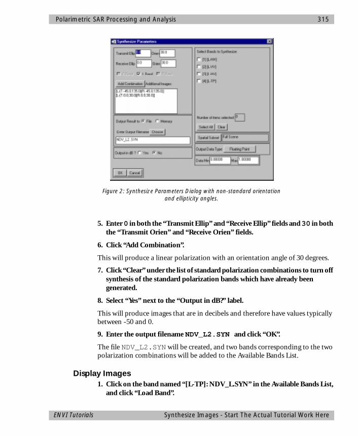
Polarimetric SAR Processing and Analysis 315
5. Enter 0 in both the “Transmit Ellip” and “Receive Ellip” fields and 30 in both the “Transmit Orien” and “Receive Orien” fields.
6. Click “Add Combination”.
This will produce a linear polarization with an orientation angle of 30 degrees.
7. Click “Clear” under the list of standard polarization combinations to turn off synthesis of the standard polarization bands which have already been generated.
8. Select “Yes” next to the “Output in dB?” label.
This will produce images that are in decibels and therefore have values typically between -50 and 0.
9. Enter the output filename NDV_L2.SYN and click “OK”.
The file NDV_L2.SYN will be created, and two bands corresponding to the two polarization combinations will be added to the Available Bands List.
Display Images1. Click on the band named “[L-TP]: NDV_L.SYN” in the Available Bands List,
and click “Load Band”.
Figure 2: Synthesize Parameters Dialog with non-standard orientation and ellipticity angles.
ENVI Tutorials Synthesize Images - Start The Actual Tutorial Work Here
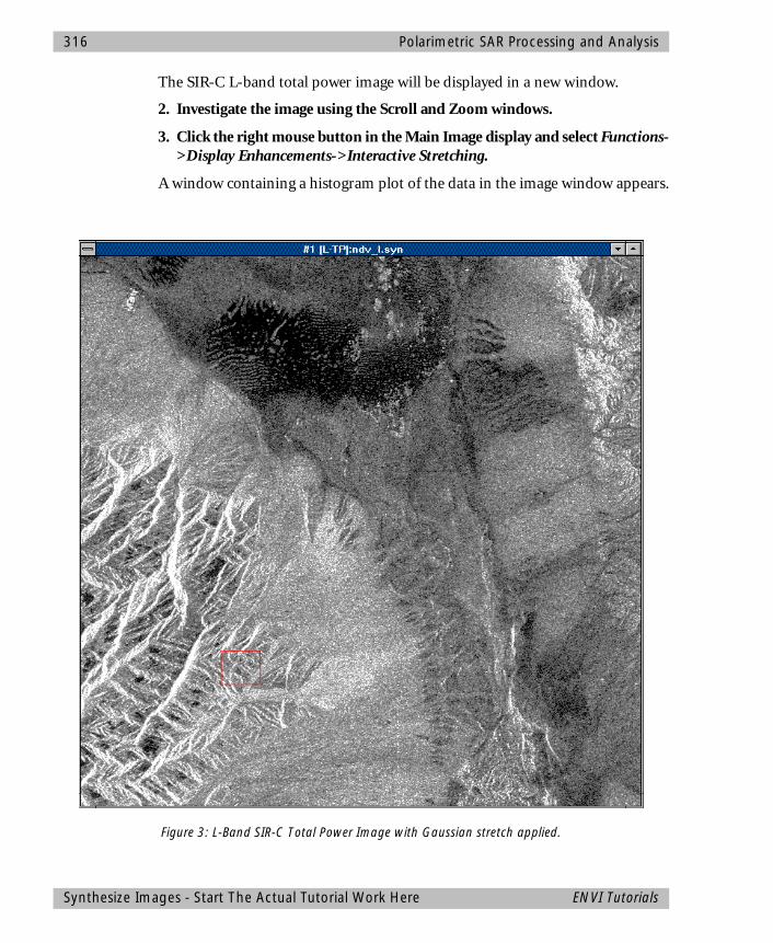
316 Polarimetric SAR Processing and Analysis
The SIR-C L-band total power image will be displayed in a new window.
2. Investigate the image using the Scroll and Zoom windows.
3. Click the right mouse button in the Main Image display and select Functions->Display Enhancements->Interactive Stretching.
A window containing a histogram plot of the data in the image window appears.
Figure 3: L-Band SIR-C Total Power Image with Gaussian stretch applied.
Synthesize Images - Start The Actual Tutorial Work Here ENVI Tutorials

Polarimetric SAR Processing and Analysis 317
The histogram plot shows the current stretch with the red and green lines on the input histogram and the corresponding DN values in the text boxes.
4. Click the left mouse button on and drag the red and green lines to change the stretch or enter the desired DN values into the appropriate fields.
5. Enter 5% in the field next to the red bar and enter 95% in the field next to the green bar.
6. Select “Gaussian” from the “Stretch Type” button menu (initially labelled “Linear”) and click “Apply”.
This will perform a gaussian stretch with a 5% low and high cut-off.
7. Also try to compare the linear and square-root stretches.
8. To display a color composite image, select the “RGB Color” toggle button in the Available Bands List.
9. Click on the “[L-HH]: ndv_l.syn”, “[L-VV]: ndv_l.syn”, and “[L-HV]: ndv_l.syn” bands.
10. Click “New” to start a new display window.
11. Click “Load RGB” to display the HH band in red, VV in green, and HV in blue.
12. Adjust the stretch as desired (Gaussian and Square Root both work well on all three bands).
13. Display the other synthesized bands as desired.
The color variations in the images are caused by variations in the radar reflectivity of the surfaces. The bright areas in the sand dunes are caused by scattering of the radar waves by vegetation (mesquite bushes). The alluvial fans show variations in surface texture due to age and composition of the rock materials.
Define ROIs for Polarization SignaturesPolarization signatures can be extracted from the SIR-C compressed scattering matrix for a Region of Interest (ROI) or a single pixel in a polarimetric radar image. ROIs are defined by selecting pixels or by drawing lines or polygons within an image.
1. Select Functions->Region of Interest->Define Region of Interest in the window containing the grayscale L-TP image.
The Region of Interest Controls dialog appears.
ENVI Tutorials Define ROIs for Polarization Signatures
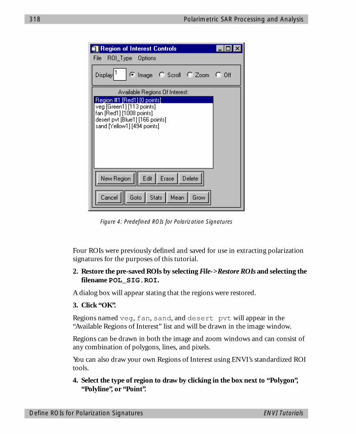
318 Polarimetric SAR Processing and Analysis
Four ROIs were previously defined and saved for use in extracting polarization signatures for the purposes of this tutorial.
2. Restore the pre-saved ROIs by selecting File->Restore ROIs and selecting the filename POL_SIG.ROI.
A dialog box will appear stating that the regions were restored.
3. Click “OK”.
Regions named veg, fan, sand, and desert pvt will appear in the “Available Regions of Interest” list and will be drawn in the image window.
Regions can be drawn in both the image and zoom windows and can consist of any combination of polygons, lines, and pixels.
You can also draw your own Regions of Interest using ENVI’s standardized ROI tools.
4. Select the type of region to draw by clicking in the box next to “Polygon”, “Polyline”, or “Point”.
Figure 4: Predefined ROIs for Polarization Signatures
Define ROIs for Polarization Signatures ENVI Tutorials

Polarimetric SAR Processing and Analysis 319
• Draw polygons by clicking the left mouse button to select the endpoints of line segments or holding down the mouse button and moving the cursor for continuous drawing.
• Click the right mouse button once to close the polygon and a second time to accept the polygon
• Polylines are drawn in the same manner as polygons.
• Click the left mouse button to define the line endpoints and click the right button to end the polyline and again to accept the polyline
• Point mode is used to select individual pixels.
• Click the left mouse button to add the pixel currently under the cursor to the ROI.
Multiple polygons, lines, and pixels may be selected for each ROI.
5. Click “New Region” to define another ROI, enter a name, and choose a color.
6. Draw a second ROI.
ROIs can be saved to a file and restored at a later time by choosing File->Save ROI in the ROI Controls dialog.
Extract Polarization SignaturesPolarization signatures are 3-D representations of the complete radar scattering characteristics of the surface for a pixel or average of pixels. They show the backscatter response at all combinations of transmit and receive polarizations and are represented as either co-polarized or cross-polarized. Co-polarized signatures have the same transmit and receive polarizations. Cross-polarized signatures have orthogonal transmit and receive polarizations. Polarization signatures are extracted from the compressed scattering matrix data using the ROIs for pixel locations. Polarization signatures are displayed in viewer windows; the figure below shows an example.
To extract your own polarization signatures:
1. Select Radar Tools->Polarimetric Tools->Extract polarization Signatures->SIR-C.
The filename NDV_L.CDP should appear in the dialog.
• If not, click “Open File” and select the filename.
2. Click “OK”.
The Polsig Parameters dialog will appear.
ENVI Tutorials Extract Polarization Signatures
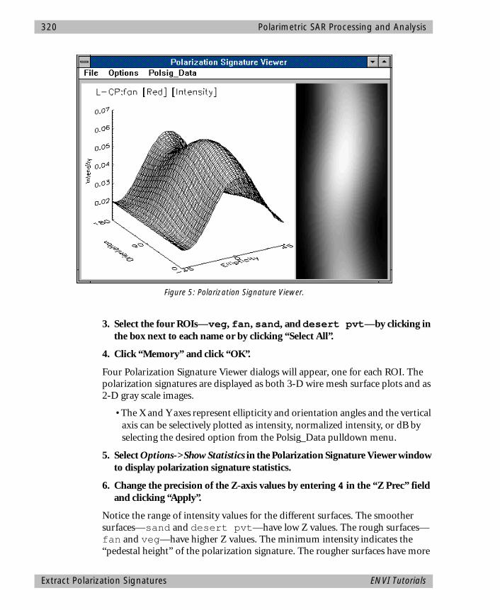
320 Polarimetric SAR Processing and Analysis
3. Select the four ROIs—veg, fan, sand, and desert pvt—by clicking in the box next to each name or by clicking “Select All”.
4. Click “Memory” and click “OK”.
Four Polarization Signature Viewer dialogs will appear, one for each ROI. The polarization signatures are displayed as both 3-D wire mesh surface plots and as 2-D gray scale images.
• The X and Y axes represent ellipticity and orientation angles and the vertical axis can be selectively plotted as intensity, normalized intensity, or dB by selecting the desired option from the Polsig_Data pulldown menu.
5. Select Options->Show Statistics in the Polarization Signature Viewer window to display polarization signature statistics.
6. Change the precision of the Z-axis values by entering 4 in the “Z Prec” field and clicking “Apply”.
Notice the range of intensity values for the different surfaces. The smoother surfaces—sand and desert pvt—have low Z values. The rough surfaces—fan and veg—have higher Z values. The minimum intensity indicates the “pedestal height” of the polarization signature. The rougher surfaces have more
Figure 5: Polarization Signature Viewer.
Extract Polarization Signatures ENVI Tutorials

Polarimetric SAR Processing and Analysis 321
multiple scattering and therefore have higher pedestal heights than the smoother surfaces. The shape of the signature also indicates the scattering characteristics. Signatures with a peak in the middle show a Bragg-type (resonance) scattering mechanism.
7. Change the Z axis by selecting Polsig_Data->Normalized from the pulldown menu.
This normalizes the signature by dividing by its maximum and plots it between 0 and 1. This representation shows the difference in pedestal heights and shapes better, but removes the absolute intensity differences.
• Alternately select Polsig_Data->Co-Pol and Cross-Pol to toggle between co-polarized and cross-polarized signatures.
8. Use the left mouse button to drag a 2-D cursor on the polarization signature image on the right side of the plot. Note the corresponding “3-D” Cursor in the polarization plot.
• The polarization signatures can be annotated by selecting the Options->Annotate Polsig.
• The signatures can be output by selecting File->Output in the Polarization Signa-ture Viewer window.
9. When you have finished examining the polarization signatures, select File->Cancel All to close all signature windows.
Use Adaptive FiltersAdaptive filters are used to reduce the speckle noise in a radar image while preserving the texture information. Statistics are calculated for each kernel and used as input into the filter allowing it to adapt to different textures within the image.
1. Select Radar Tools->Adaptive Filters->Gamma.
The Gamma Filter Input File dialog will appear with a list of open files. The filters can be run on an entire file or an individual band.
2. Click on the arrow toggle button next to the label “Select By File” to toggle to “Select By Band” and list the bands in the files.
3. Select the band “[L-HH]:NDV_L.SYN” and click “OK”.
The Gamma Filter Parameters dialog will appear.
ENVI Tutorials Use Adaptive Filters

322 Polarimetric SAR Processing and Analysis
4. Use a filter size of 3 and the “default number of looks” of 1 and output the result to memory by selecting the “Memory” toggle button.
5. Click “OK”.
The resulting image name will appear in the Available Bands List as “Gamma ([L-HH]: NDV_L.SYN)”.
Display the Filter Result1. Display the result of the filter by selecting the “Gray Scale” toggle button and
selecting the band name in the Available Bands List.
2. Click “New” to start a new display window and click “Load Band”.
3. Select Functions->Display Enhancements->Default (quick)->Quick Square Root in the Main window to perform a Square Root stretch on the image.
You can use dynamic overlays to compare the results of the Gamma filter to the original image.
4. Display the original band by selecting “[L-HH]: NDV_L.SYN” in the Available Bands List, clicking “New” and “Load Band”.
5. Perform a quick Square Root stretch on this image as well.
6. Select Functions->Link->Link Displays.
7. The Link Displays dialog will appear.
8. Make sure that “Yes” appears only next to the names of the two displays that contain the Gamma filtered and original images and click “OK”.
Dynamic overlay is activated automatically when the windows are linked.
9. Click the left mouse button in either image to cause a small portion of the second linked image (the overlay) to appear in the first image (the base).
The overlay is active in both windows simultaneously and in the Zoom window.
10. Move the overlay by clicking and holding the left mouse button and moving the cursor.
11. Change the size of the overlay by pressing the middle mouse button and dragging the corner of the overlay to the desired location.
12. Compare the Gamma Filter image to the original data.
13. Turn the dynamic overlay feature off by selecting functions->Link->Unlink Displays or Dynamic Overlay Off in the Main window.
Use Adaptive Filters ENVI Tutorials
Polarimetric SAR Processing and Analysis 323
Perform Slant-to-Ground Range TransformationSlant range radar data have a geometric distortion in the range direction. The true or ground range pixel sizes vary across the range direction because of the changing incidence angles. This geometric distortion is corrected by resampling the slant range data to create ground range pixels that are a fixed size. The slant-to-ground range transformation requires information about the instrument orientation. For SIR-C data, the necessary information is found in the CEOS header.
1. Select Radar Tools->Slant to Ground Range->SIR-C.
2. When the Enter SIR-C Parameters Filename dialog appears, select the file NDV_L.CDP.
The Slant Range Correction Input File dialog will appear.
3. Select the file NDV_L.SYN and click “OK”.
The Slant to Ground Range Correction Dialog will appear and all of the pertinent information will be filled in from the CEOS header in the .CDP file.
4. Enter 13.32 in the “Output pixel size” field to generate square ground-range pixels.
5. Select “Bilinear” as the resampling option, enter NDV_GR.IMG as the output filename, and click “OK”.
The input image is resampled to 1152 13.32m sized square pixels.
6. Display this image and compare it with the slant range image.
Use Texture AnalysisTexture is the measure of the spatial variation in the grey levels in the image as a function of scale. It is calculated within a processing window of user-selected size. The texture measures demonstrated in this tutorial are Occurrence Measures, including Data Range, Mean, Variance, Entropy, and Skewness. These terms are explained in the ENVI User’s Guide and on-line help. Texture is best calculated for radar data that has not had any resampling or filtering applied.
1. Select Radar Tools->Texture Filters->Occurrence Measures.
2. When the Texture Input File dialog appears, click the “Select by Band” toggle button and select the band “[L-HH]: NDV_L.SYN” and click OK.
3. In the Occurrence Texture Parameters dialog, deselect all of the Textures to Compute except for Data Range, change the Processing Window Rows and Cols to 7 x 7, enter an output filename NDV_HH.TEX, and click OK.
ENVI Tutorials Perform Slant-to-Ground Range Transformation

324 Polarimetric SAR Processing and Analysis
An ENVI Status Window will appear and after a short wait the new band will be listed in the Available Bands List.
Create Color-coded Texture MapDisplay the resulting Data Range texture image by clicking on the band name Data Range:[L-HH] in the Available Bands List and clicking “Load Band”.
1. Perform a quick square root stretch on the image.
2. Select Functions->Color Mapping->Density Slice in the Main Image display.
3. Apply the default ranges by clicking on Apply. Examine this image with respect to the original data using image linking and dynamic overlays.
4. Now select Functions->Interactive Analysis->Cursor Location/Value in the Main window and look at the Data Range values while roaming around the image.
5. Try creating your own density sliced image or use the predetermined color-coded density slice TEXTURE.DSR saved for your use by selecting File->Restore in the Density Slice dialog, selecting the file TEXTURE.DSR and clicking Open, and then Apply.
This density slice shows the various textures in the image in distinct colors.
Display and density slice some of the other texture measures and use dynamic overlays to compare to each other and the original data.
Create an Image-Map for Output1. With the Data Range texture measure displayed, add a border around the
image to place a key and text annotation.
2. Select Functions->Overlays->Annotation in the main window.
3. When the Annotation dialog appears, select Options->Set Display Borders.
4. Enter 100 in the upper text boxes, select a border color of White, and click “OK”.
This will make a 100 pixel white border at the top of the image.
5. Position the Main Image indicator box in the Scroll window at the top of the image to display the portion of the image with border.
6. Place a title at the top of the image by entering a title into the text field in the center of the dialog.
Create an Image-Map for Output ENVI Tutorials

Polarimetric SAR Processing and Analysis 325
7. Enter 16 in the “Size” field to change the font size and change the color to Black.
8. Place the title on the image by using the left mouse button to position it and clicking the right button to fix the location.
Multiple text items can be placed on the image in this manner and the font size, type, color, and thickness can be changed.
9. Put a color table ramp in the top border of the image for a color-code key by selecting Object->Color Ramp in the Annotation dialog.
10. Enter “Min” and “Max” values of 0 and 255 respectively, set “Inc” to 4, and the Font size to 14 to annotate the Color Ramp.
11. Position the color ramp using the left mouse button and fix the location by clicking the right mouse button.
12. Add any other objects desired to the image using the annotation dialog.
13. Save the image to a PostScript file by selecting Functions->Output Display->Postscript File.
14. Enter an output filename or let the name default to ndv_hh.ps. and click “OK”.
15. Optionally, output directly to your printer by selecting Functions->Output Display->Printer.
Exit ENVIWhen you have finished your ENVI session, click “Quit” or “Exit” on the ENVI Main Menu.
ENVI Tutorials Create an Image-Map for Output
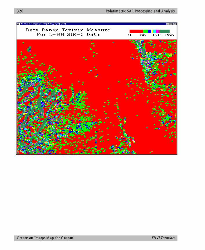
326 Polarimetric SAR Processing and Analysis
Create an Image-Map for Output ENVI Tutorials

ENVI Tutorial #17
Analysis of DEMs and TOPSAR
The following topics are covered in this tutorial:
Overview of This Tutorial ......................................................................................328Files Used in This Tutorial ......................................................................................328Background - TOPSAR and DEMs..........................................................................329Displaying the Data and Converting to Physical Parameters ..................................329Synthesizing the P- and L-band Data ....................................................................334Analysis of JPL Polarimetric SAR Data.....................................................................334Displaying and Analyzing DEMs............................................................................339Image-Map Output...............................................................................................348Summary ..............................................................................................................348
327
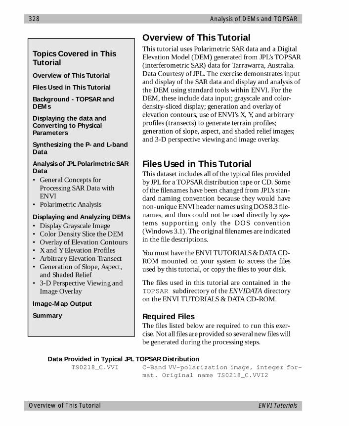
328 Analysis of DEMs and TOPSAR
Overview of This TutorialThis tutorial uses Polarimetric SAR data and a Digital Elevation Model (DEM) generated from JPL’s TOPSAR (interferometric SAR) data for Tarrawarra, Australia. Data Courtesy of JPL. The exercise demonstrates input and display of the SAR data and display and analysis of the DEM using standard tools within ENVI. For the DEM, these include data input; grayscale and color-density-sliced display; generation and overlay of elevation contours, use of ENVI’s X, Y, and arbitrary profiles (transects) to generate terrain profiles; generation of slope, aspect, and shaded relief images; and 3-D perspective viewing and image overlay.
Files Used in This TutorialThis dataset includes all of the typical files providedby JPL for a TOPSAR distribution tape or CD. Someof the filenames have been changed from JPL’s stan-dard naming convention because they would havenon-unique ENVI header names using DOS 8.3 file-names, and thus could not be used directly by sys-tems supporting only the DOS convention(Windows 3.1). The original filenames are indicatedin the file descriptions.
You must have the ENVI TUTORIALS & DATA CD-ROM mounted on your system to access the filesused by this tutorial, or copy the files to your disk.
The files used in this tutorial are contained in theTOPSAR subdirectory of the ENVIDATA directoryon the ENVI TUTORIALS & DATA CD-ROM.
Required FilesThe files listed below are required to run this exer-cise. Not all files are provided so several new files willbe generated during the processing steps.
Data Provided in Typical JPL TOPSAR DistributionTS0218_C.VVI C-Band VV-polarization image, integer for-
mat. Original name TS0218_C.VVI2
Topics Covered in This Tutorial
Overview of This Tutorial
Files Used in This Tutorial
Background - TOPSAR and DEMs
Displaying the data and Converting to Physical Parameters
Synthesizing the P- and L-band Data
Analysis of JPL Polarimetric SAR Data• General Concepts for
Processing SAR Data with ENVI
• Polarimetric Analysis
Displaying and Analyzing DEMs• Display Grayscale Image• Color Density Slice the DEM• Overlay of Elevation Contours• X and Y Elevation Profiles• Arbitrary Elevation Transect• Generation of Slope, Aspect,
and Shaded Relief• 3-D Perspective Viewing and
Image Overlay
Image-Map Output
Summary
Overview of This Tutorial ENVI Tutorials
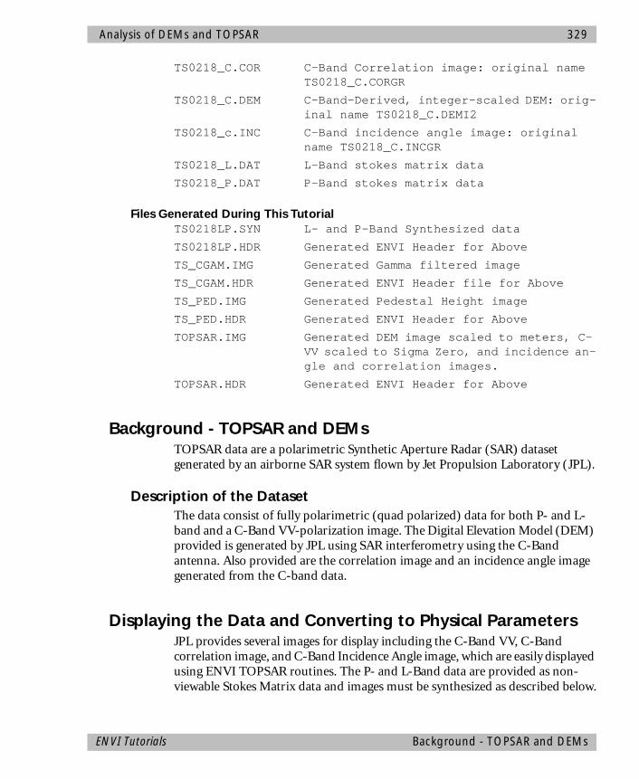
Analysis of DEMs and TOPSAR 329
TS0218_C.COR C-Band Correlation image: original name TS0218_C.CORGR
TS0218_C.DEM C-Band-Derived, integer-scaled DEM: orig-inal name TS0218_C.DEMI2
TS0218_c.INC C-Band incidence angle image: original name TS0218_C.INCGR
TS0218_L.DAT L-Band stokes matrix data
TS0218_P.DAT P-Band stokes matrix data
Files Generated During This TutorialTS0218LP.SYN L- and P-Band Synthesized data
TS0218LP.HDR Generated ENVI Header for Above
TS_CGAM.IMG Generated Gamma filtered image
TS_CGAM.HDR Generated ENVI Header file for Above
TS_PED.IMG Generated Pedestal Height image
TS_PED.HDR Generated ENVI Header for Above
TOPSAR.IMG Generated DEM image scaled to meters, C-VV scaled to Sigma Zero, and incidence an-gle and correlation images.
TOPSAR.HDR Generated ENVI Header for Above
Background - TOPSAR and DEMsTOPSAR data are a polarimetric Synthetic Aperture Radar (SAR) dataset generated by an airborne SAR system flown by Jet Propulsion Laboratory (JPL).
Description of the DatasetThe data consist of fully polarimetric (quad polarized) data for both P- and L-band and a C-Band VV-polarization image. The Digital Elevation Model (DEM) provided is generated by JPL using SAR interferometry using the C-Band antenna. Also provided are the correlation image and an incidence angle image generated from the C-band data.
Displaying the Data and Converting to Physical ParametersJPL provides several images for display including the C-Band VV, C-Band correlation image, and C-Band Incidence Angle image, which are easily displayed using ENVI TOPSAR routines. The P- and L-Band data are provided as non-viewable Stokes Matrix data and images must be synthesized as described below.
ENVI Tutorials Background - TOPSAR and DEMs
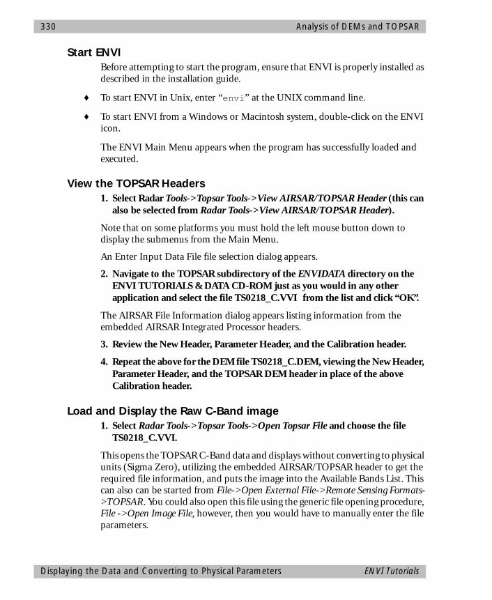
330 Analysis of DEMs and TOPSAR
Start ENVIBefore attempting to start the program, ensure that ENVI is properly installed as described in the installation guide.
♦ To start ENVI in Unix, enter “envi” at the UNIX command line.
♦ To start ENVI from a Windows or Macintosh system, double-click on the ENVI icon.
The ENVI Main Menu appears when the program has successfully loaded and executed.
View the TOPSAR Headers1. Select Radar Tools->Topsar Tools->View AIRSAR/TOPSAR Header (this can
also be selected from Radar Tools->View AIRSAR/TOPSAR Header).
Note that on some platforms you must hold the left mouse button down to display the submenus from the Main Menu.
An Enter Input Data File file selection dialog appears.
2. Navigate to the TOPSAR subdirectory of the ENVIDATA directory on the ENVI TUTORIALS & DATA CD-ROM just as you would in any other application and select the file TS0218_C.VVI from the list and click “OK”.
The AIRSAR File Information dialog appears listing information from the embedded AIRSAR Integrated Processor headers.
3. Review the New Header, Parameter Header, and the Calibration header.
4. Repeat the above for the DEM file TS0218_C.DEM, viewing the New Header, Parameter Header, and the TOPSAR DEM header in place of the above Calibration header.
Load and Display the Raw C-Band image1. Select Radar Tools->Topsar Tools->Open Topsar File and choose the file
TS0218_C.VVI.
This opens the TOPSAR C-Band data and displays without converting to physical units (Sigma Zero), utilizing the embedded AIRSAR/TOPSAR header to get the required file information, and puts the image into the Available Bands List. This can also can be started from File->Open External File->Remote Sensing Formats->TOPSAR. You could also open this file using the generic file opening procedure, File ->Open Image File, however, then you would have to manually enter the file parameters.
Displaying the Data and Converting to Physical Parameters ENVI Tutorials
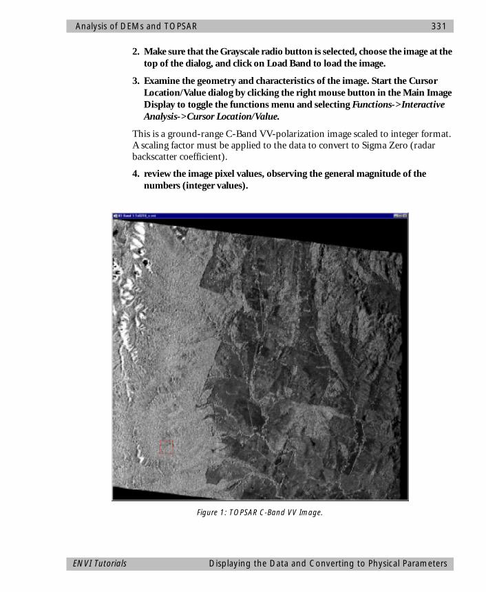
Analysis of DEMs and TOPSAR 331
2. Make sure that the Grayscale radio button is selected, choose the image at the top of the dialog, and click on Load Band to load the image.
3. Examine the geometry and characteristics of the image. Start the Cursor Location/Value dialog by clicking the right mouse button in the Main Image Display to toggle the functions menu and selecting Functions->Interactive Analysis->Cursor Location/Value.
This is a ground-range C-Band VV-polarization image scaled to integer format. A scaling factor must be applied to the data to convert to Sigma Zero (radar backscatter coefficient).
4. review the image pixel values, observing the general magnitude of the numbers (integer values).
Figure 1: TOPSAR C-Band VV Image.
ENVI Tutorials Displaying the Data and Converting to Physical Parameters
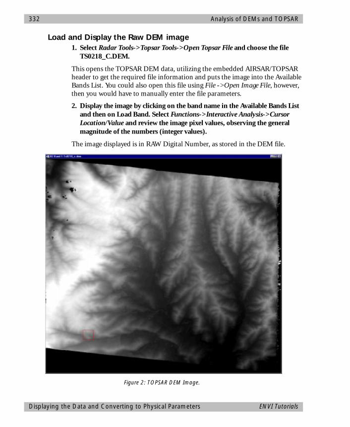
332 Analysis of DEMs and TOPSAR
Load and Display the Raw DEM image1. Select Radar Tools->Topsar Tools->Open Topsar File and choose the file
TS0218_C.DEM.
This opens the TOPSAR DEM data, utilizing the embedded AIRSAR/TOPSAR header to get the required file information and puts the image into the Available Bands List. You could also open this file using File ->Open Image File, however, then you would have to manually enter the file parameters.
2. Display the image by clicking on the band name in the Available Bands List and then on Load Band. Select Functions->Interactive Analysis->Cursor Location/Value and review the image pixel values, observing the general magnitude of the numbers (integer values).
The image displayed is in RAW Digital Number, as stored in the DEM file.
Figure 2: TOPSAR DEM Image.
Displaying the Data and Converting to Physical Parameters ENVI Tutorials
Analysis of DEMs and TOPSAR 333
EN
3. Select Functions->Link->Link Displays and use ENVI’s dynamic overlay capabilities to compare the two images.
Convert the C-Band data to Sigma Zero and DEM to meters1. Select Radar Tools->Topsar Tools->Convert Topsar Data and choose
the file TS0218_C.VVI.
ENVI automatically identifies all of the TOPSAR data present in this dataset based on the TOPSAR file naming convention. The VV Polarization, Correlation, Incidence Angle, and DEM images will be opened. The C-VV data will automatically be converted to Sigma Zero and the DEM to meters based upon values present in the TOPSAR headers.
2. Enter the output filename TOPSAR.IMG and click OK to start the conversion.
The four images are placed in the available bands list.
3. Display the C-VV Sigma Zero image by clicking on the VV Polarization band name in the Available Bands List, clicking New, and then on Load Band. Select Functions->Interactive Analysis->Cursor Location/Value and review the image pixel values, observing the general magnitude of the numbers (Sigma Zero).
4. Select Functions->Link->Link Displays and use ENVI’s dynamic overlay capabilities to compare the two C-VV images (Raw vs Sigma Zero).
5. Display the DEM (meters) image by clicking on the DEM (m) band name in the Available Bands List, clicking New, and then on Load Band. Toggle on the Functions menu if not present by clicking the right mouse button in the main image window, then select Functions->Interactive Analysis->Cursor Location/Value and review the image pixel values, observing the general magnitude of the numbers (Elevation in meters). Note the large negative number (approximately -2911) associated with holes in the DEM and the image border. These are not valid elevations and these areas should be excluded from analysis using ENVI’s masking functions.
6. Select Functions->Link->Link Displays and use ENVI’s dynamic overlay capabilities to compare the two DEM images (Raw vs Elevation in meters).
VI Tutorials Displaying the Data and Converting to Physical Parameters
334 Analysis of DEMs and TOPSAR
Synthesizing the P- and L-band DataBoth the L-Band and P-Band data are distributed by JPL in compressed Stokes Matrix format. These data can not be displayed directly by most image processing systems. ENVI provides utilities to decompress the data and synthesize to image format.
1. Select Radar Tools->Polarimetric Tools->Decompress/Synthesize Images->Synthesize AIRSAR Images or Radar Tools->Decompress/Synthesize Images->Synthesize AIRSAR Images from the ENVI Main menu.
2. Click on Open File in the Input Stokes Matrix Files dialog, select the file TS02218_L.DAT and click Open.
Both the L and P band Stokes Matrix file names will be entered into the dialog.
3. Click OK to start the Synthesize Parameters dialog.
The “standard” polarization bands, L-HH, L-VV, L-HV, L-TP (total power), P-HH, P-VV, P-HV, and P-TP (total power) will be automatically entered into the dialog.
4. If additional polarizations are desired, enter the Transmit and Receive Ellipticity and Orientation angles into the appropriate text boxes in the upper left part of the dialog and click on Add Combination.
5. Select “Byte” as the Output Data Type from the pulldown menu originally labeled “Floating Point”, enter the output filename TS0218LP.SYN, and click OK to synthesize the images.
6. Select one or more of the synthesized bands to display as grayscale or RGB images, load using the Available Bands List, and display.
7. Compare the L-Band and C-Band VV data to the C-Band VV data using image linking and dynamic overlays.
Analysis of JPL Polarimetric SAR DataThis section of the tutorial describes some of the analysis options for general analysis of SAR data as well as selected polarimetric analysis capabilities. For additional SAR processing information see the ENVI User’s Guide.
General Concepts for processing SAR with ENVIMost standard ENVI processing functions are inherently radar capable including all display capabilities, stretching, color manipulations, classification, registration, filters, geometric rectification, etc. Specific Radar menu items are also included under the Radar Tools menu for specific ENVI routines that are
Synthesizing the P- and L-band Data ENVI Tutorials
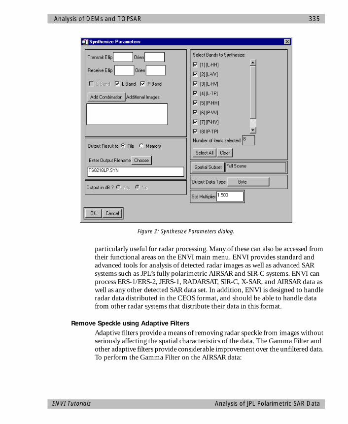
Analysis of DEMs and TOPSAR 335
particularly useful for radar processing. Many of these can also be accessed from their functional areas on the ENVI main menu. ENVI provides standard and advanced tools for analysis of detected radar images as well as advanced SAR systems such as JPL’s fully polarimetric AIRSAR and SIR-C systems. ENVI can process ERS-1/ERS-2, JERS-1, RADARSAT, SIR-C, X-SAR, and AIRSAR data as well as any other detected SAR data set. In addition, ENVI is designed to handle radar data distributed in the CEOS format, and should be able to handle data from other radar systems that distribute their data in this format.
Remove Speckle using Adaptive FiltersAdaptive filters provide a means of removing radar speckle from images without seriously affecting the spatial characteristics of the data. The Gamma Filter and other adaptive filters provide considerable improvement over the unfiltered data. To perform the Gamma Filter on the AIRSAR data:
Figure 3: Synthesize Parameters dialog.
ENVI Tutorials Analysis of JPL Polarimetric SAR Data
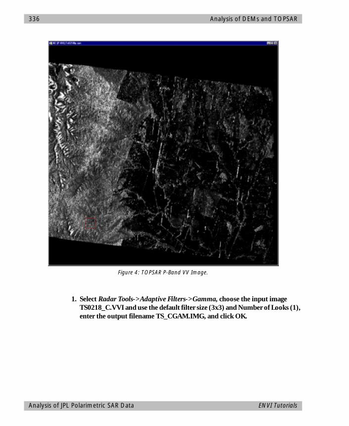
336 Analysis of DEMs and TOPSAR
1. Select Radar Tools->Adaptive Filters->Gamma, choose the input image TS0218_C.VVI and use the default filter size (3x3) and Number of Looks (1), enter the output filename TS_CGAM.IMG, and click OK.
Figure 4: TOPSAR P-Band VV Image.
Analysis of JPL Polarimetric SAR Data ENVI Tutorials

Analysis of DEMs and TOPSAR 337
Edge EnhancementA Laplacian Filter can be used to enhance edges in SAR data and other data types. This is a convolution filter with a kernel (for a 5 x 5 filter) of:
Of course, applying the kernel in this fashion strongly enhances the edges and causes loss of most of the radiometric information.
1. From the ENVI Main Menu, select Filter ->Convolution ->Laplacian.
One solution to this problem is to “add-back” part of the original image.
2. To apply add-back to a filtered image, select Filter->Convolution->Laplacian, and enter the add-back factor (between 0 and 1 where 1 is 100%) in the Convolution Parameters dialog.
Compare Images using Linked Images and Dynamic OverlayCompare images generated above to each other and the original data using ENVI's dynamic overlay capabilities. To compare the images using Dynamic Overlay:
1. Display the two images in separate displays and contrast stretch as described above.
2. Click the right mouse button in one of the displays to toggle the Functions menu and select Functions ->Link ->Link Displays.
3. Click “OK” to link the two images and compare by dragging the dynamic overlay with the left mouse button.
Polarimetric AnalysisENVI provides a full suite of tools for analyzing Polarimetric SAR data. These include generation and display of specific polarization images, a phase image, and pedestal height image as well as extraction of polarization signatures and generation of a scattering classification image.
0 0 -1 0 0
0 -1 -2 -1 0
-1 -2 16 -2 -1
0 -1 -2 -1 0
0 0 -1 0 0
ENVI Tutorials Analysis of JPL Polarimetric SAR Data

338 Analysis of DEMs and TOPSAR
Display Multifrequency, Polarimetric SAR ImagesThe synthesized images produced above form the basis for image analysis of polarimetric data.
1. Display one of the synthesized images by selecting the band [L-HH}:TS0218LP.SYN in the Available Bands List and clicking on Load Band.
2. Start an animation by choosing Functions->Interactive Analysis->Animation. Click on the check boxes for the two total power images to deselect and then OK to start the animation. Observe the different frequencies and polarizations and compare the SAR response for various materials to determine a 3-band combination that will maximize “spectral contrast”.
3. When finished, click Cancel to end the animation.
4. Load a multifrequency, multipolarizaiton AIRSAR image into the display as an RGB image using your selected bands from above, or load the P-HH, L-HH, and the C-VV image as RGB and observe the color differences associated with various materials. Experiment with different contrast stretches using both the Main Display and the Zoom Windows to maximize color differences in the image.
Examine Polarization SignaturesPolarization signatures are 3D representations of the complete scattering characteristics for a single pixel or ROI in terms of the orientation angle and ellipticity angle of the transmitted and received radar waves. These signatures can be used to observe the scattering characteristics of materials and surfaces and to determine what polarization images to generate to maximize image contrast between materials as viewed in the SAR data.
1. Position the cursor over an area that appeared to change significantly in the animation by clicking at the desired location in the Main Image Display window using the middle mouse button.
2. Choose Interactive Analysis->Polarization Signatures->AIRSAR, click on the Open File button, and choose the L-Band Stokes Matrix data TS0218_L.DAT and click Open.
Both the L-Band and P-Band Stokes Matrix filenames will be entered into the Input Stokes Matrix Files dialog.
3. Click OK to start the Polarization Signature Viewer window and choose Options->Extract Current Pixel to extract an L-Band polarization signature for the current pixel. Choose Frequency->P to display the corresponding P-Band polarization signature, then click in the signature in the left portion of
Analysis of JPL Polarimetric SAR Data ENVI Tutorials
Analysis of DEMs and TOPSAR 339
the plot using the left mouse button to toggle different surface plotting options. Be sure to display and compare the cross-polarized signature.
4. Choose Options->Show Statistics to view polarization signature information and statistics. Click Cancel to quit this function.
5. Click and drag using the left mouse button in the image on the right side of the plot to display interactive 2-D, 3-D cursor. Read the cursor values in the lower left corner of the plot. Observe the maximum contrast orientation and ellipticity angles in the plot and optionally synthesize and display an image with these parameters as described above.
6. Select Polsig_Data->Option, where Option is one of the available display methods. Be sure to display and compare the cross-polarized signature. Select File->Cancel to exit the function.
Pedestal Height Image1. Generate a pedestal height image for the AIRSAR data by choosing Radar
Tools->Polarimetric Tools->Pedestal Height Image->AIRSAR, clicking OK in the Input Stokes Matrix Files dialog, entering the output filename TS_PED.IMG and clicking OK.
2. Display the image by clicking on the band name in the Available Bands List and clicking on Load Band.
This image provides a measure of the amount of multiple scatter of the radar wave for every pixel by averaging the following four polarization combinations: Orientation 0 degrees, Ellipticity -45 degrees; Orientation 90 degrees, Ellipticity -45 degrees; Orientation 0 degrees, Ellipticity 45 degrees; Orientation 90 degrees, Ellipticity 45 degrees. A higher pedestal height value in the image indicates greater multiple scattering, generally a rougher surface.
3. Select Interactive Analysis->Cursor Location/Value to start the Cursor Location/Value window and examine the pedestal height values for this image.
Displaying and Analyzing DEMsThis portion of the tutorial describes ENVI’s tools for processing and analyzing Digital Elevation Models. While this tutorial refers specifically to the TOPSAR DEM, all of these methods and tools are fully applicable to any DEM data set.
ENVI Tutorials Displaying and Analyzing DEMs

340 Analysis of DEMs and TOPSAR
Display the DEM Converted to Meters1. If not already displayed, display the band DEM (m) from the generated file
TOPSAR.IMG. Use Radar Tools->TOPSAR Tools->View AIRSAR/TOPSAR Header to examine the DEM header parameters.
1. Select Functions->Interactive Analysis->Cursor Location/Value and examine the pixel values of the DEM.
This DEM has had a scaling function applied to convert these data to physical parameters; the elevation in meters. The formula for this conversion is on page 21 of the AIRSAR Integrated Processor Documentation, version 0.01, May 1995. The required information for this conversion is obtained from the TOPSAR DEM header, in this case, consisting of an ELEVATION INCREMENT of 0.1 and the ELEVATION OFFSET of 365.6. Also note that after this conversion, bad pixels (borders, radar shadows in the DEM, etc) will have the value -2911.099. You probably will want to generate a mask for these areas using ENVI masking capabilities to set these values to zero (see the ENVI User’s Guide for details).
X and Y Elevation ProfilesENVI provides tools for extracting elevation profiles along either the X or Y directions. Move these two plots off to the side of the image display so you can see them while moving the cursor in the display.
1. Select Functions->Profiles->X Profile and then Functions->Profiles->Y Profile to extract the profiles for the two directions.
Figure 5: TOPSAR horizontal and vertical DEM topographic profiles.
Displaying and Analyzing DEMs ENVI Tutorials

Analysis of DEMs and TOPSAR 341
2. Click and drag using the left mouse button to generate new elevation profiles when the left mouse button is released. The position of the red bar in the X and Y profiles marks the position of the center of the Zoom window along the profile. For continuous updating, click and drag using the middle mouse button.
3. Close the two profiles by choosing Basic Tools->Display Controls->Close All Plot Windows.
Arbitrary Elevation TransectENVI also allows extraction of elevation profiles along multiple arbitrary transects.
1. Select Functions->Profiles->Arbitrary Profile (Transect) to extract a profile along an arbitrary transect.
2. Click using the left mouse button in the Main Display Window to draw each segment of the desired transect. You can hold down the left mouse button and draw if desired.
3. Click the right mouse button once to close the last line segment and a second time to extract the profile.
Figure 6: TOPSAR DEM Arbitrary Transects.
ENVI Tutorials Displaying and Analyzing DEMs
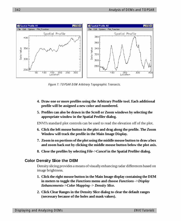
342 Analysis of DEMs and TOPSAR
4. Draw one or more profiles using the Arbitrary Profile tool. Each additional profile will be assigned a new color and numbered.
5. Profiles can also be drawn in the Scroll or Zoom windows by selecting the appropriate window in the Spatial Profiler dialog.
ENVI’s standard plot controls can be used to read the elevation off of the plot.
6. Click the left mouse button in the plot and drag along the profile. The Zoom Window will track the profile in the Main Image Display.
7. Zoom in on portions of the plot using the middle mouse button to draw a box and zoom back out by clicking the middle mouse button below the plot axis.
8. Close the profiles by selecting File->Cancel in the Spatial Profiler dialog.
Color Density Slice the DEMDensity slicing provides a means of visually enhancing radar differences based on image brightness.
1. Click the right mouse button in the Main Image display containing the DEM in meters to toggle the Functions menu and choose Functions ->Display Enhancements->Color Mapping -> Density Slice.
2. Click Clear Ranges in the Density Slice dialog to clear the default ranges (necessary because of the holes and mask values).
Figure 7: TOPSAR DEM Arbitrary Topographic Transects.
Displaying and Analyzing DEMs ENVI Tutorials
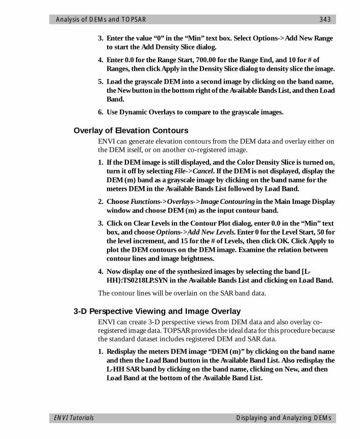
Analysis of DEMs and TOPSAR 343
3. Enter the value “0” in the “Min” text box. Select Options->Add New Range to start the Add Density Slice dialog.
4. Enter 0.0 for the Range Start, 700.00 for the Range End, and 10 for # of Ranges, then click Apply in the Density Slice dialog to density slice the image.
5. Load the grayscale DEM into a second image by clicking on the band name, the New button in the bottom right of the Available Bands List, and then Load Band.
6. Use Dynamic Overlays to compare to the grayscale images.
Overlay of Elevation ContoursENVI can generate elevation contours from the DEM data and overlay either on the DEM itself, or on another co-registered image.
1. If the DEM image is still displayed, and the Color Density Slice is turned on, turn it off by selecting File->Cancel. If the DEM is not displayed, display the DEM (m) band as a grayscale image by clicking on the band name for the meters DEM in the Available Bands List followed by Load Band.
2. Choose Functions->Overlays->Image Contouring in the Main Image Display window and choose DEM (m) as the input contour band.
3. Click on Clear Levels in the Contour Plot dialog, enter 0.0 in the “Min” text box, and choose Options->Add New Levels. Enter 0 for the Level Start, 50 for the level increment, and 15 for the # of Levels, then click OK. Click Apply to plot the DEM contours on the DEM image. Examine the relation between contour lines and image brightness.
4. Now display one of the synthesized images by selecting the band [L-HH}:TS0218LP.SYN in the Available Bands List and clicking on Load Band.
The contour lines will be overlain on the SAR band data.
3-D Perspective Viewing and Image OverlayENVI can create 3-D perspective views from DEM data and also overlay co-registered image data. TOPSAR provides the ideal data for this procedure because the standard dataset includes registered DEM and SAR data.
1. Redisplay the meters DEM image “DEM (m)” by clicking on the band name and then the Load Band button in the Available Band List. Also redisplay the L-HH SAR band by clicking on the band name, clicking on New, and then Load Band at the bottom of the Available Band List.
ENVI Tutorials Displaying and Analyzing DEMs
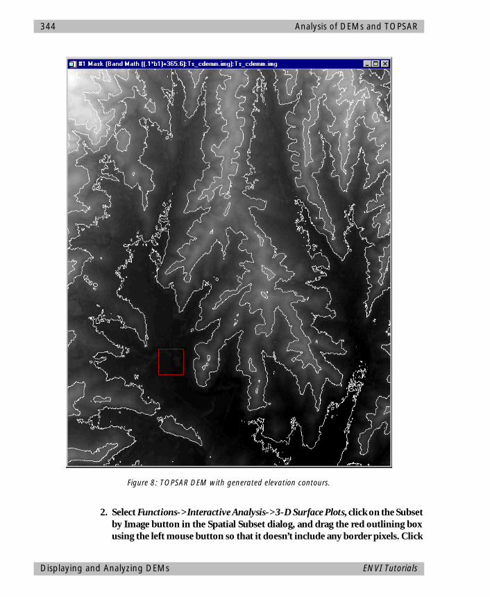
344 Analysis of DEMs and TOPSAR
2. Select Functions->Interactive Analysis->3-D Surface Plots, click on the Subset by Image button in the Spatial Subset dialog, and drag the red outlining box using the left mouse button so that it doesn’t include any border pixels. Click
Figure 8: TOPSAR DEM with generated elevation contours.
Displaying and Analyzing DEMs ENVI Tutorials
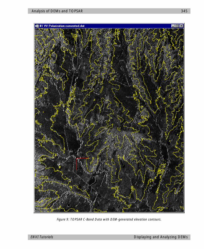
Analysis of DEMs and TOPSAR 345
Figure 9: TOPSAR C-Band Data with DEM-generated elevation contours.
ENVI Tutorials Displaying and Analyzing DEMs
346 Analysis of DEMs and TOPSAR
OK in the Subset Function dialog and then OK again in the Spatial Subset dialog.
A wire-frame 3-D surface of the DEM is drawn in a Surface Plot window.
3. Choose Edit->Plot Parameters from the Surface Plot menu bar and enter the values 75 and 45 for the AX and AZ parameters respectively. Click on Apply at the bottom of the dialog to redraw the 3-D surface.
4. Select Surface->Shaded Surface from the Surface Plot menu bar and choose Display 1 (the DEM) as the overlay image in the Overlay dialog.
This overlays the DEM as a grayscale image on the 3-D perspective
5. Select Surface->Shaded Surface from the Surface Plot menu bar and choose Display 2(the SAR image) as the overlay image in the Overlay dialog.
This overlays the L-HH SAR image on the DEM as a grayscale image.
Figure 10: Wire-Mesh perspective view of TOPSAR DEM.
Displaying and Analyzing DEMs ENVI Tutorials
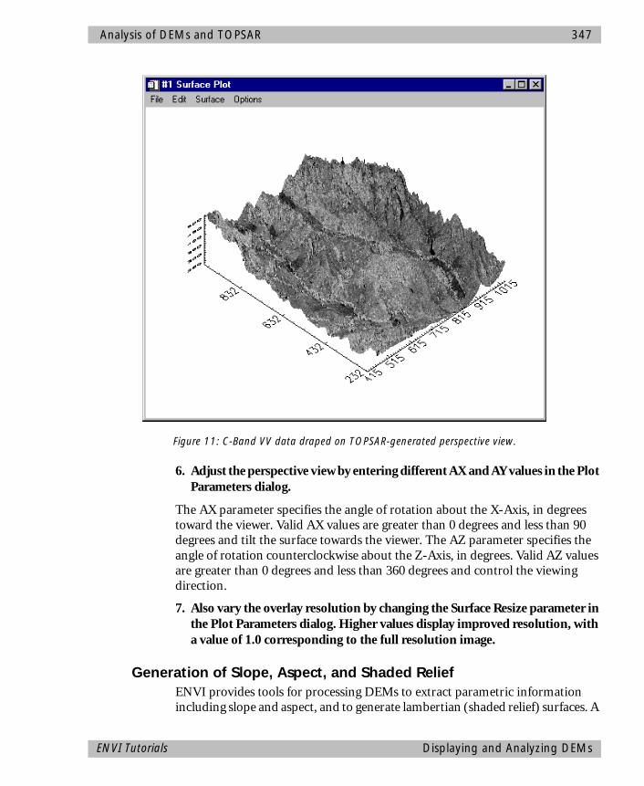
Analysis of DEMs and TOPSAR 347
6. Adjust the perspective view by entering different AX and AY values in the Plot Parameters dialog.
The AX parameter specifies the angle of rotation about the X-Axis, in degrees toward the viewer. Valid AX values are greater than 0 degrees and less than 90 degrees and tilt the surface towards the viewer. The AZ parameter specifies the angle of rotation counterclockwise about the Z-Axis, in degrees. Valid AZ values are greater than 0 degrees and less than 360 degrees and control the viewing direction.
7. Also vary the overlay resolution by changing the Surface Resize parameter in the Plot Parameters dialog. Higher values display improved resolution, with a value of 1.0 corresponding to the full resolution image.
Generation of Slope, Aspect, and Shaded ReliefENVI provides tools for processing DEMs to extract parametric information including slope and aspect, and to generate lambertian (shaded relief) surfaces. A
Figure 11: C-Band VV data draped on TOPSAR-generated perspective view.
ENVI Tutorials Displaying and Analyzing DEMs
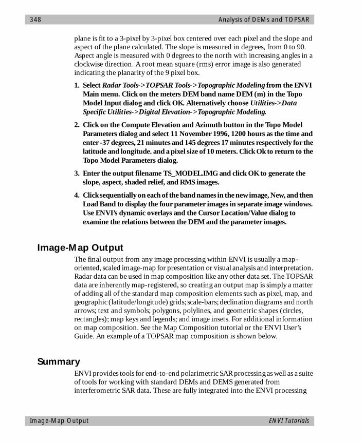
348 Analysis of DEMs and TOPSAR
plane is fit to a 3-pixel by 3-pixel box centered over each pixel and the slope and aspect of the plane calculated. The slope is measured in degrees, from 0 to 90. Aspect angle is measured with 0 degrees to the north with increasing angles in a clockwise direction. A root mean square (rms) error image is also generated indicating the planarity of the 9 pixel box.
1. Select Radar Tools->TOPSAR Tools->Topographic Modeling from the ENVI Main menu. Click on the meters DEM band name DEM (m) in the Topo Model Input dialog and click OK. Alternatively choose Utilities->Data Specific Utilities->Digital Elevation->Topographic Modeling.
2. Click on the Compute Elevation and Azimuth button in the Topo Model Parameters dialog and select 11 November 1996, 1200 hours as the time and enter -37 degrees, 21 minutes and 145 degrees 17 minutes respectively for the latitude and longitude. and a pixel size of 10 meters. Click Ok to return to the Topo Model Parameters dialog.
3. Enter the output filename TS_MODEL.IMG and click OK to generate the slope, aspect, shaded relief, and RMS images.
4. Click sequentially on each of the band names in the new image, New, and then Load Band to display the four parameter images in separate image windows. Use ENVI’s dynamic overlays and the Cursor Location/Value dialog to examine the relations between the DEM and the parameter images.
Image-Map OutputThe final output from any image processing within ENVI is usually a map-oriented, scaled image-map for presentation or visual analysis and interpretation. Radar data can be used in map composition like any other data set. The TOPSAR data are inherently map-registered, so creating an output map is simply a matter of adding all of the standard map composition elements such as pixel, map, and geographic (latitude/longitude) grids; scale-bars; declination diagrams and north arrows; text and symbols; polygons, polylines, and geometric shapes (circles, rectangles); map keys and legends; and image insets. For additional information on map composition. See the Map Composition tutorial or the ENVI User’s Guide. An example of a TOPSAR map composition is shown below.
SummaryENVI provides tools for end-to-end polarimetric SAR processing as well as a suite of tools for working with standard DEMs and DEMS generated from interferometric SAR data. These are fully integrated into the ENVI processing
Image-Map Output ENVI Tutorials
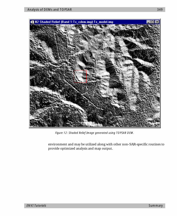
Analysis of DEMs and TOPSAR 349
environment and may be utilized along with other non-SAR-specific routines to provide optimized analysis and map output.
Figure 12: Shaded Relief Image generated using TOPSAR DEM.
ENVI Tutorials Summary
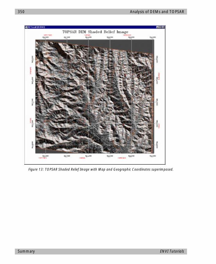
350 Analysis of DEMs and TOPSAR
Figure 13: TOPSAR Shaded Relief Image with Map and Geographic Coordinates superimposed.
Summary ENVI Tutorials

ENVI Tutorial #18
Introduction to ENVI User Functions
The following topics are covered in this tutorial:
Overview of This Tutorial ......................................................................................352Background - Programming in ENVI .....................................................................352User Defined Band Math Routines.........................................................................353Creating a User Function ......................................................................................358Running the User Function....................................................................................362Write the Tiling Routines .......................................................................................363
351
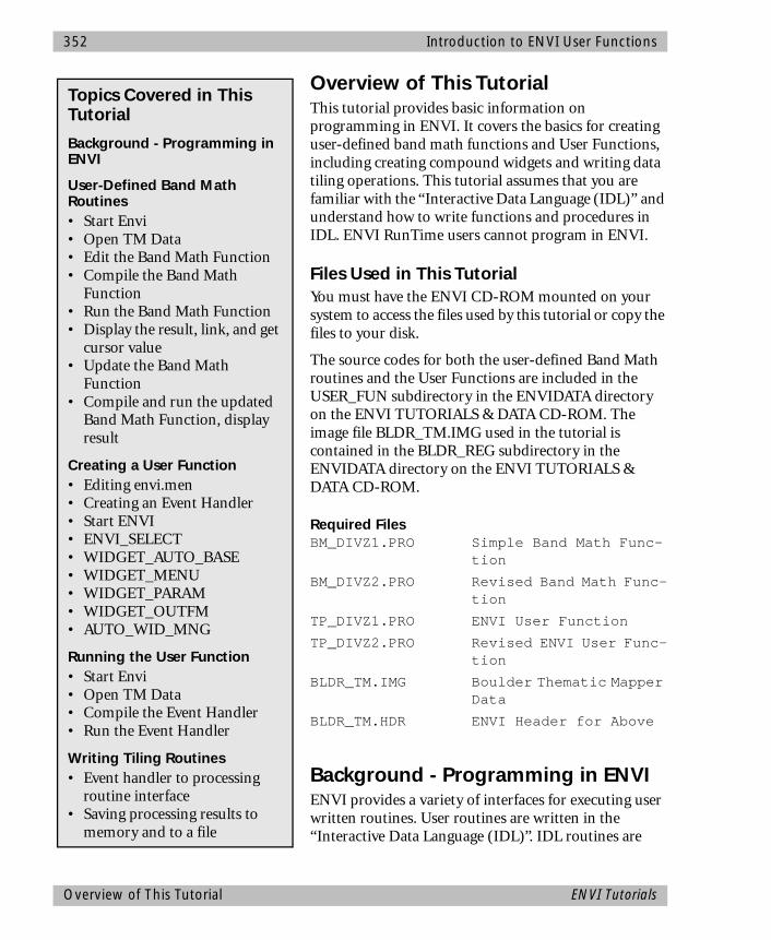
352 Introduction to ENVI User Functions
Overview of This TutorialThis tutorial provides basic information on programming in ENVI. It covers the basics for creating user-defined band math functions and User Functions, including creating compound widgets and writing data tiling operations. This tutorial assumes that you are familiar with the “Interactive Data Language (IDL)” and understand how to write functions and procedures in IDL. ENVI RunTime users cannot program in ENVI.
Files Used in This TutorialYou must have the ENVI CD-ROM mounted on your system to access the files used by this tutorial or copy the files to your disk.
The source codes for both the user-defined Band Math routines and the User Functions are included in the USER_FUN subdirectory in the ENVIDATA directory on the ENVI TUTORIALS & DATA CD-ROM. The image file BLDR_TM.IMG used in the tutorial is contained in the BLDR_REG subdirectory in the ENVIDATA directory on the ENVI TUTORIALS & DATA CD-ROM.
Required Files BM_DIVZ1.PRO Simple Band Math Func-
tion
BM_DIVZ2.PRO Revised Band Math Func-tion
TP_DIVZ1.PRO ENVI User Function
TP_DIVZ2.PRO Revised ENVI User Func-tion
BLDR_TM.IMG Boulder Thematic Mapper Data
BLDR_TM.HDR ENVI Header for Above
Background - Programming in ENVIENVI provides a variety of interfaces for executing user written routines. User routines are written in the “Interactive Data Language (IDL)”. IDL routines are
Topics Covered in This Tutorial
Background - Programming in ENVI
User-Defined Band Math Routines• Start Envi• Open TM Data• Edit the Band Math Function• Compile the Band Math
Function• Run the Band Math Function• Display the result, link, and get
cursor value• Update the Band Math
Function• Compile and run the updated
Band Math Function, display result
Creating a User Function• Editing envi.men• Creating an Event Handler• Start ENVI• ENVI_SELECT• WIDGET_AUTO_BASE• WIDGET_MENU• WIDGET_PARAM• WIDGET_OUTFM• AUTO_WID_MNG
Running the User Function• Start Envi• Open TM Data• Compile the Event Handler• Run the Event Handler
Writing Tiling Routines• Event handler to processing
routine interface• Saving processing results to
memory and to a file
Overview of This Tutorial ENVI Tutorials

Introduction to ENVI User Functions 353
written as functions or procedures and named with a .pro extension. This tutorial shows examples of two of these techniques - Band Math and User Functions. For descriptions of the ENVI programming functions used in this tutorial, see the ENVI User’s Guide or on-line help.
ENVI processes data spatially or spectrally depending on the requirements of the function and on the input file storage format. If a function only operates either spatially or spectrally then the data must be accessed accordingly. However, if a process can be performed either spatially or spectrally, then ENVI operates on the data based on the file storage format. The three file storage formats that ENVI uses are Band Sequential (BSQ), Band Interleave by Line (BIL), or Band Interleave by Pixel (BIP) (See the ENVI User’s Guide, on-line help, or ENVI Tutorials).
ENVI allows processing of image data larger than available memory. This is accomplished by breaking the data up into usable pieces or “tiles”, processing the tiles separately, then reassembling the tiles into the output image. A tile is a piece of data processed in memory by ENVI. The size of a spatial tile is determined by the ENVI configuration item image tile size and is set by the user to optimize memory usage without exceeding the computer’s physical memory size. Spatial tiles always include all the samples being processed and as many lines as possible. Spectral tiles on the other hand, are defined by the number of samples (ns) and the number of bands (nb) being processed. A BIL spectral tile is (ns, nb) and a BIP spectral tile is (nb, ns). Spectral tiles will always be this size and are unrelated to the set image tile size.
The basic process for a tiling operation in ENVI is as follows:
Initialize the ENVI tilesLoop on the number of tiles request the tile process the tile [write result of the processing to disk or memory]
end loop[Enter the data into Available Bands List]
User Defined Band Math RoutinesThis portion of the exercise will familiarize you with editing and compiling a .pro file (an IDL program). The compiled function is executed using ENVI’s Band Math routine. Band math uses ENVI’s tiling capabilities for handling large images. You will create a simple band math function that performs a mathematical expression using two bands. The optional keyword CHECK will
ENVI Tutorials User Defined Band Math Routines
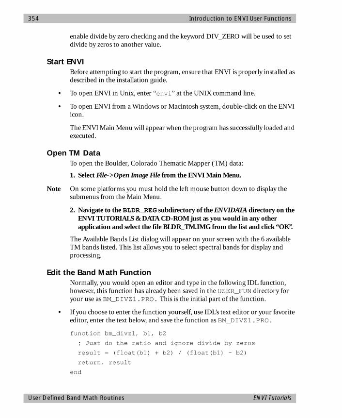
354 Introduction to ENVI User Functions
enable divide by zero checking and the keyword DIV_ZERO will be used to set divide by zeros to another value.
Start ENVIBefore attempting to start the program, ensure that ENVI is properly installed as described in the installation guide.
• To open ENVI in Unix, enter “envi” at the UNIX command line.
• To open ENVI from a Windows or Macintosh system, double-click on the ENVI icon.
The ENVI Main Menu will appear when the program has successfully loaded and executed.
Open TM DataTo open the Boulder, Colorado Thematic Mapper (TM) data:
1. Select File->Open Image File from the ENVI Main Menu.
Note On some platforms you must hold the left mouse button down to display the submenus from the Main Menu.
2. Navigate to the BLDR_REG subdirectory of the ENVIDATA directory on the ENVI TUTORIALS & DATA CD-ROM just as you would in any other application and select the file BLDR_TM.IMG from the list and click “OK”.
The Available Bands List dialog will appear on your screen with the 6 available TM bands listed. This list allows you to select spectral bands for display and processing.
Edit the Band Math FunctionNormally, you would open an editor and type in the following IDL function, however, this function has already been saved in the USER_FUN directory for your use as BM_DIVZ1.PRO. This is the initial part of the function.
• If you choose to enter the function yourself, use IDL’s text editor or your favorite editor, enter the text below, and save the function as BM_DIVZ1.PRO.
function bm_divz1, b1, b2
; Just do the ratio and ignore divide by zeros
result = (float(b1) + b2) / (float(b1) - b2)
return, result
end
User Defined Band Math Routines ENVI Tutorials

Introduction to ENVI User Functions 355
Compile the Band Math FunctionTo compile the newly created function:
1. Select System->Compile Module from the ENVI Main Menu.
2. When the Enter Module Filename dialog appears, navigate to the location of the saved function, BM_DIVZ1.PRO, and select the file.
3. To make sure that the function compiled without errors, look in the IDL output log window.
On the PC and MAC this is the OUTPUT LOG window and under UNIX it is the shell window ENVI was started from. The following line will appear if the module compiled successfully.
% Compiled module BM_DIVZ1
4. Edit and fix any errors for modules that did not compile successfully and recompile as above.
Run the Band Math Function1. To run the compiled function select Basic Tools->Band Math from the ENVI
Main Menu.
2. When the Band Math dialog appears, enter the following in the “Enter an expression:” input text box:
bm_divz1(b1,b2)
3. Click “OK”.
4. When the Variable/Band Pairings dialog appears, click on “B1” in the “Variables used in expression” list widget.
5. From the “Available Bands List:” list widget, click on “Band 2”.
Repeat the same process to pair B2 with TM Band 3.
6. Select “B2” from the “Variables used in expression” list widget.
7. From the “Available Bands List:” list widget, select “Band 3”.
Now the “Variables used in expression:” should show the following.
B1- Band 2:bldr_tm.img
B2 - Band 3:bldr_tm.img
8. Click “OK”.
9. When the Band Math Parameters dialog appears, select the “Output Result to File” toggle button, enter an output filename, and click “OK”.
ENVI Tutorials User Defined Band Math Routines
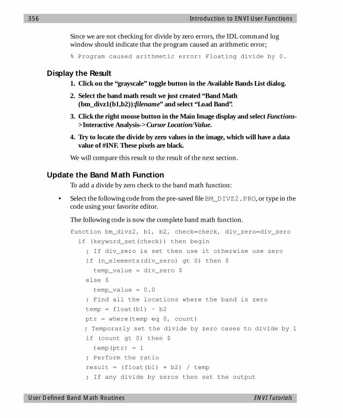
356 Introduction to ENVI User Functions
Since we are not checking for divide by zero errors, the IDL command log window should indicate that the program caused an arithmetic error;
% Program caused arithmetic error: Floating divide by 0.
Display the Result1. Click on the “grayscale” toggle button in the Available Bands List dialog.
2. Select the band math result we just created “Band Math (bm_divz1(b1,b2)):filename” and select “Load Band”.
3. Click the right mouse button in the Main Image display and select Functions->Interactive Analysis->Cursor Location/Value.
4. Try to locate the divide by zero values in the image, which will have a data value of #INF. These pixels are black.
We will compare this result to the result of the next section.
Update the Band Math FunctionTo add a divide by zero check to the band math function:
• Select the following code from the pre-saved file BM_DIVZ2.PRO, or type in the code using your favorite editor.
The following code is now the complete band math function.
function bm_divz2, b1, b2, check=check, div_zero=div_zero
if (keyword_set(check)) then begin
; If div_zero is set then use it otherwise use zero
if (n_elements(div_zero) gt 0) then $
temp_value = div_zero $
else $
temp_value = 0.0
; Find all the locations where the band is zero
temp = float(b1) - b2
ptr = where(temp eq 0, count)
; Temporarly set the divide by zero cases to divide by 1
if (count gt 0) then $
temp(ptr) = 1
; Perform the ratio
result = (float(b1) + b2) / temp
; If any divide by zeros then set the output
User Defined Band Math Routines ENVI Tutorials

Introduction to ENVI User Functions 357
if (count gt 0) then $
result(ptr) = temp_value
endif else begin
; Just do the ratio and ignore divide by zeros
result = (float(b1) + b2) / (float(b1) - b2)
endelse
return, result
end
Compile the Band Math FunctionTo compile the updated function:
1. Select System->Compile Module from the ENVI Main Menu.
2. When the Enter Module Filename appears, navigate to the location of the saved function, BM_DIVZ2.PRO, and select the file.
3. To make sure that the function compiled, look in the IDL output log window.
On the PC and MAC this is the OUTPUT LOG window and under UNIX it is shell window ENVI was started from. The following line will appear if the module compiled successfully.
% Compiled module BM_DIVZ2
4. Edit and fix any errors for modules that did not compile successfully.
Run the Band Math FunctionThe new function can now check for divide by zeros and can set them to an error value. To run the compiled function:
1. Select Basic Tools->Band Math.
2. When the Band Math dialog appears, enter the following in the “Enter an expression:” input text box:
bm_divz2(b1,b2, /check, div_zero=1.0)
3. Click “OK”.
4. When the Variable/Band Pairings dialog appears, click on “B1” in the “Variables used in expression” list widget.
5. From the “Available Bands List:” list widget, click on “Band 2”.
Repeat the same process to pair B2 with TM Band 3.
6. Select “B2” from the “Variables used in expression” list widget.
ENVI Tutorials User Defined Band Math Routines
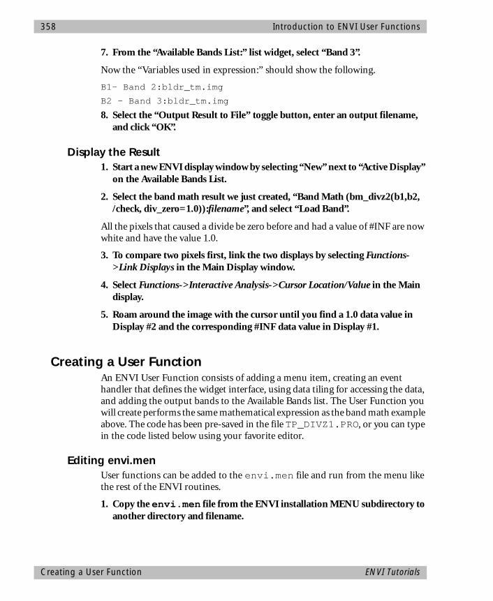
358 Introduction to ENVI User Functions
7. From the “Available Bands List:” list widget, select “Band 3”.
Now the “Variables used in expression:” should show the following.
B1- Band 2:bldr_tm.img
B2 - Band 3:bldr_tm.img
8. Select the “Output Result to File” toggle button, enter an output filename, and click “OK”.
Display the Result1. Start a new ENVI display window by selecting “New” next to “Active Display”
on the Available Bands List.
2. Select the band math result we just created, “Band Math (bm_divz2(b1,b2, /check, div_zero=1.0)):filename”, and select “Load Band”.
All the pixels that caused a divide be zero before and had a value of #INF are now white and have the value 1.0.
3. To compare two pixels first, link the two displays by selecting Functions->Link Displays in the Main Display window.
4. Select Functions->Interactive Analysis->Cursor Location/Value in the Main display.
5. Roam around the image with the cursor until you find a 1.0 data value in Display #2 and the corresponding #INF data value in Display #1.
Creating a User FunctionAn ENVI User Function consists of adding a menu item, creating an event handler that defines the widget interface, using data tiling for accessing the data, and adding the output bands to the Available Bands list. The User Function you will create performs the same mathematical expression as the band math example above. The code has been pre-saved in the file TP_DIVZ1.PRO, or you can type in the code listed below using your favorite editor.
Editing envi.menUser functions can be added to the envi.men file and run from the menu like the rest of the ENVI routines.
1. Copy the envi.men file from the ENVI installation MENU subdirectory to another directory and filename.
Creating a User Function ENVI Tutorials

Introduction to ENVI User Functions 359
2. Enter the new filename (including the directory path) in the “default envi menu file” parameter in the envi.cfg file.
Exit ENVI so that you can update the envi.men file to include your new routine.
3. To quit your ENVI session, click “Quit” or “Exit” on the ENVI Main Menu, then type “ exit” at the IDL command prompt.
4. Edit your new envi menu file and locate the line:
1 {User Functions}
5. Directly below this line enter the following two lines for the new menu items:
2 {User Band Ratio1} {user ratio} {tp_divz1}
2 {User Band Ratio2} {user ratio} {tp_divz2}
where 2 indicates the menu level, {User Band Ratio} is the menu item name, {user ratio} is the name of the uvalue, and {tp_divz1} or {tp_divz2} is the name of the event handler.
6. Close and save the new envi menu file.
Creating an Event Handler This portion of the exercise will familiarize you with creating ENVI event handlers for user defined functions. You will use the ENVI file selection function and ENVI’s compound widgets.
Edit the event handler1. Enter the following code using your text editor or use the file included in the
USER_FUN directory under the filename TP_DIVZ1.PRO.
The first thing to do in the routine is to extract the uvalue and compare it the uvalue in the envi menu file.
After receiving the uvalue the event handler selects the input file. ENVI_SELECT is used for file selection and spatial and spectral subsetting. Returned from ENVI_SELECT are the input file id (FID), the band dimensions (DIMS), and the selected bands (POS). If the returned FID equals -1 then the “Cancel” button was selected and the event handler must exit.
Since the processing routine is performing the same mathematical expression as the band math example, we need to make sure that at lease two bands are selected. If the improper number of bands are selected then ENVI_ERROR is used to give a warning message and the event handler exits.
ENVI Tutorials Creating a User Function

360 Introduction to ENVI User Functions
Input parameters entered on the command line in the Band Math exercise are now entered using ENVI compound widgets.
• Use WIDGET_AUTO_BASE to create a widget base which allows auto-manage-ment of widget events.
• Use row and column bases for positioning the compound widgets WIDGET_MENU and WIDGET_PARAM to replace the keywords in the Band Math example.
• WIDGET_MENU creates the “Check for divide by 0?” using an exclusive list to make a “Yes/No” toggle button.
• WIDGET_PARAM accepts an input value that is used as the replacement for the divide by zero.
• WIDGET_PARAM accepts a floating point number (DT=4) with three digits past the decimal points (FIELDS=3) with a default value of zero (DEFAULT=0.0).
• Finally, WIDGET_OUTFM is used to prompt for the output filename or memory option.
• Each of the compound widgets set the keyword /auto giving AUTO_WID_MNG the responsibility of managing the compound widgets.
• AUTO_WID_MNG returns a structure with the tag names defined by the uvalue of each compound widget.
• In addition, the structure contains the tag accept, which is set to one if the you select “OK” and zero if the “Cancel” button is selected.
In this example, we print the selections for “Check for divide by 0?” and the “Divide by zero value”. The next exercise will use the same event handler but pass the arguments to the tile processing routine.
pro tp_divz1, ev
widget_control, ev.id, get_uvalue=uvalue
if (uvalue eq ’user ratio’) then begin
envi_select, title=’Ratio Input File’, fid=fid, dims=dims, $
pos=pos
if (fid eq -1) then return
; We will just do a ratio of the first two band
Creating a User Function ENVI Tutorials
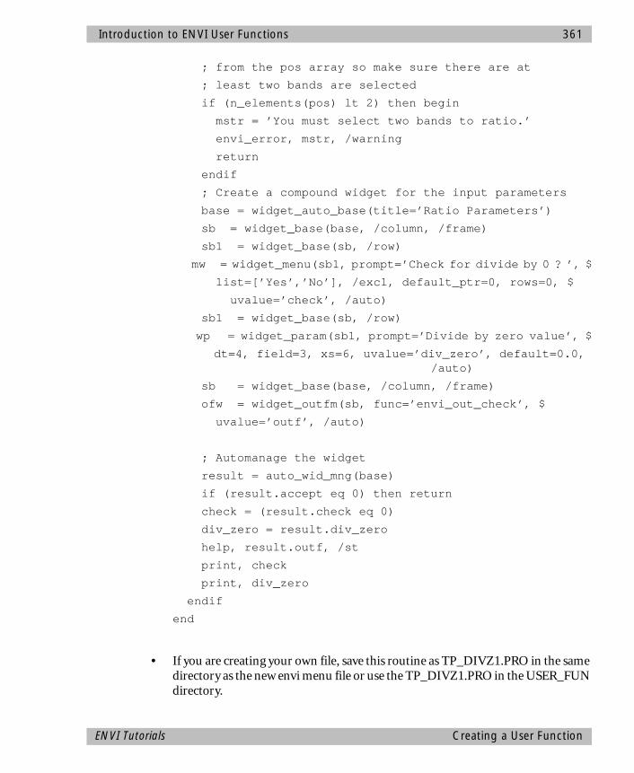
Introduction to ENVI User Functions 361
; from the pos array so make sure there are at
; least two bands are selected
if (n_elements(pos) lt 2) then begin
mstr = ’You must select two bands to ratio.’
envi_error, mstr, /warning
return
endif
; Create a compound widget for the input parameters
base = widget_auto_base(title=’Ratio Parameters’)
sb = widget_base(base, /column, /frame)
sb1 = widget_base(sb, /row)
mw = widget_menu(sb1, prompt=’Check for divide by 0 ? ’, $
list=[’Yes’,’No’], /excl, default_ptr=0, rows=0, $
uvalue=’check’, /auto)
sb1 = widget_base(sb, /row)
wp = widget_param(sb1, prompt=’Divide by zero value’, $
dt=4, field=3, xs=6, uvalue=’div_zero’, default=0.0, /auto)
sb = widget_base(base, /column, /frame)
ofw = widget_outfm(sb, func=’envi_out_check’, $
uvalue=’outf’, /auto)
; Automanage the widget
result = auto_wid_mng(base)
if (result.accept eq 0) then return
check = (result.check eq 0)
div_zero = result.div_zero
help, result.outf, /st
print, check
print, div_zero
endif
end
• If you are creating your own file, save this routine as TP_DIVZ1.PRO in the same directory as the new envi menu file or use the TP_DIVZ1.PRO in the USER_FUN directory.
ENVI Tutorials Creating a User Function
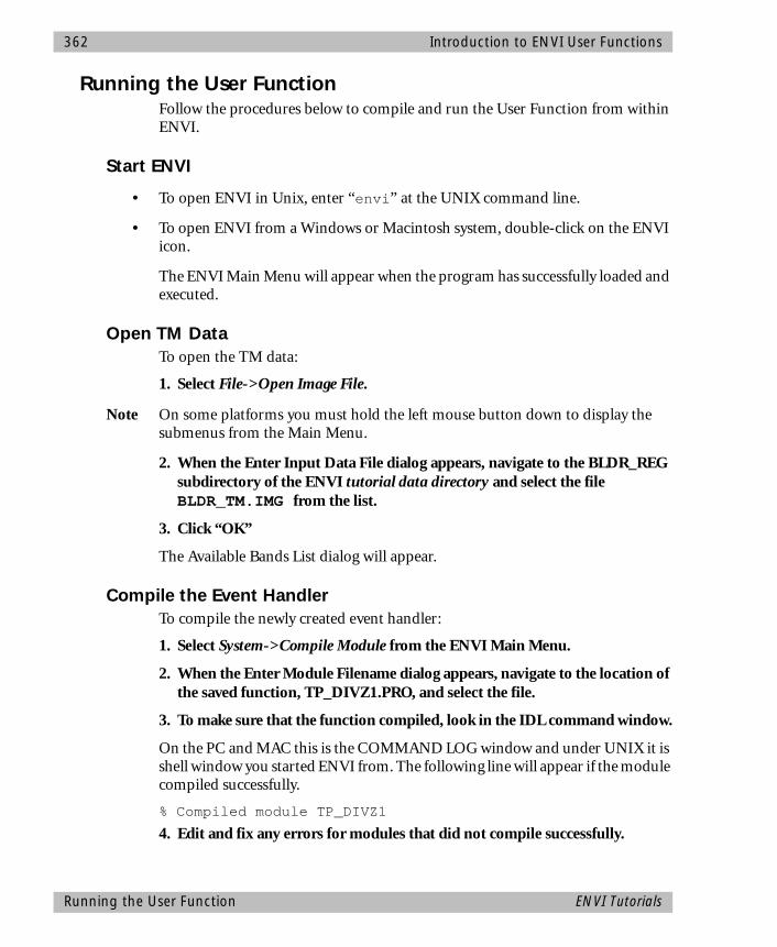
362 Introduction to ENVI User Functions
Running the User FunctionFollow the procedures below to compile and run the User Function from within ENVI.
Start ENVI
• To open ENVI in Unix, enter “envi” at the UNIX command line.
• To open ENVI from a Windows or Macintosh system, double-click on the ENVI icon.
The ENVI Main Menu will appear when the program has successfully loaded and executed.
Open TM DataTo open the TM data:
1. Select File->Open Image File.
Note On some platforms you must hold the left mouse button down to display the submenus from the Main Menu.
2. When the Enter Input Data File dialog appears, navigate to the BLDR_REG subdirectory of the ENVI tutorial data directory and select the file BLDR_TM.IMG from the list.
3. Click “OK”
The Available Bands List dialog will appear.
Compile the Event HandlerTo compile the newly created event handler:
1. Select System->Compile Module from the ENVI Main Menu.
2. When the Enter Module Filename dialog appears, navigate to the location of the saved function, TP_DIVZ1.PRO, and select the file.
3. To make sure that the function compiled, look in the IDL command window.
On the PC and MAC this is the COMMAND LOG window and under UNIX it is shell window you started ENVI from. The following line will appear if the module compiled successfully.
% Compiled module TP_DIVZ1
4. Edit and fix any errors for modules that did not compile successfully.
Running the User Function ENVI Tutorials
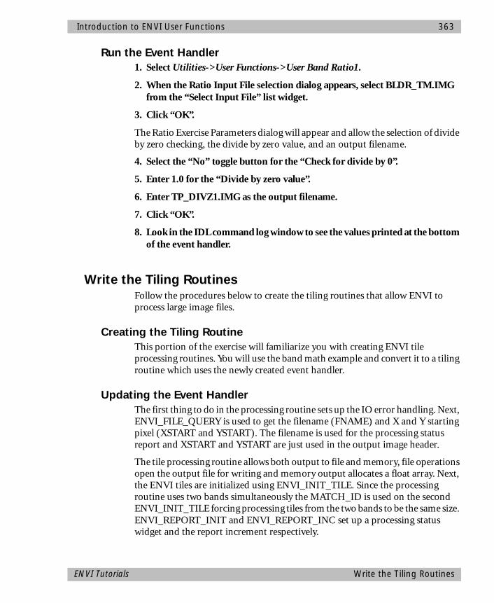
Introduction to ENVI User Functions 363
Run the Event Handler1. Select Utilities->User Functions->User Band Ratio1.
2. When the Ratio Input File selection dialog appears, select BLDR_TM.IMG from the “Select Input File” list widget.
3. Click “OK”.
The Ratio Exercise Parameters dialog will appear and allow the selection of divide by zero checking, the divide by zero value, and an output filename.
4. Select the “No” toggle button for the “Check for divide by 0”.
5. Enter 1.0 for the “Divide by zero value”.
6. Enter TP_DIVZ1.IMG as the output filename.
7. Click “OK”.
8. Look in the IDL command log window to see the values printed at the bottom of the event handler.
Write the Tiling RoutinesFollow the procedures below to create the tiling routines that allow ENVI to process large image files.
Creating the Tiling RoutineThis portion of the exercise will familiarize you with creating ENVI tile processing routines. You will use the band math example and convert it to a tiling routine which uses the newly created event handler.
Updating the Event HandlerThe first thing to do in the processing routine sets up the IO error handling. Next, ENVI_FILE_QUERY is used to get the filename (FNAME) and X and Y starting pixel (XSTART and YSTART). The filename is used for the processing status report and XSTART and YSTART are just used in the output image header.
The tile processing routine allows both output to file and memory, file operations open the output file for writing and memory output allocates a float array. Next, the ENVI tiles are initialized using ENVI_INIT_TILE. Since the processing routine uses two bands simultaneously the MATCH_ID is used on the second ENVI_INIT_TILE forcing processing tiles from the two bands to be the same size. ENVI_REPORT_INIT and ENVI_REPORT_INC set up a processing status widget and the report increment respectively.
ENVI Tutorials Write the Tiling Routines
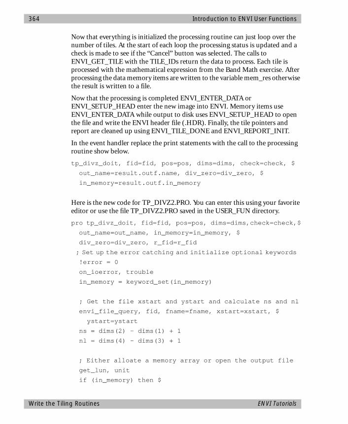
364 Introduction to ENVI User Functions
Now that everything is initialized the processing routine can just loop over the number of tiles. At the start of each loop the processing status is updated and a check is made to see if the “Cancel” button was selected. The calls to ENVI_GET_TILE with the TILE_IDs return the data to process. Each tile is processed with the mathematical expression from the Band Math exercise. After processing the data memory items are written to the variable mem_res otherwise the result is written to a file.
Now that the processing is completed ENVI_ENTER_DATA or ENVI_SETUP_HEAD enter the new image into ENVI. Memory items use ENVI_ENTER_DATA while output to disk uses ENVI_SETUP_HEAD to open the file and write the ENVI header file (.HDR). Finally, the tile pointers and report are cleaned up using ENVI_TILE_DONE and ENVI_REPORT_INIT.
In the event handler replace the print statements with the call to the processing routine show below.
tp_divz_doit, fid=fid, pos=pos, dims=dims, check=check, $
out_name=result.outf.name, div_zero=div_zero, $
in_memory=result.outf.in_memory
Here is the new code for TP_DIVZ2.PRO. You can enter this using your favorite editor or use the file TP_DIVZ2.PRO saved in the USER_FUN directory.
pro tp_divz_doit, fid=fid, pos=pos, dims=dims,check=check,$
out_name=out_name, in_memory=in_memory, $
div_zero=div_zero, r_fid=r_fid
; Set up the error catching and initialize optional keywords
!error = 0
on_ioerror, trouble
in_memory = keyword_set(in_memory)
; Get the file xstart and ystart and calculate ns and nl
envi_file_query, fid, fname=fname, xstart=xstart, $
ystart=ystart
ns = dims(2) - dims(1) + 1
nl = dims(4) - dims(3) + 1
; Either alloate a memory array or open the output file
get_lun, unit
if (in_memory) then $
Write the Tiling Routines ENVI Tutorials
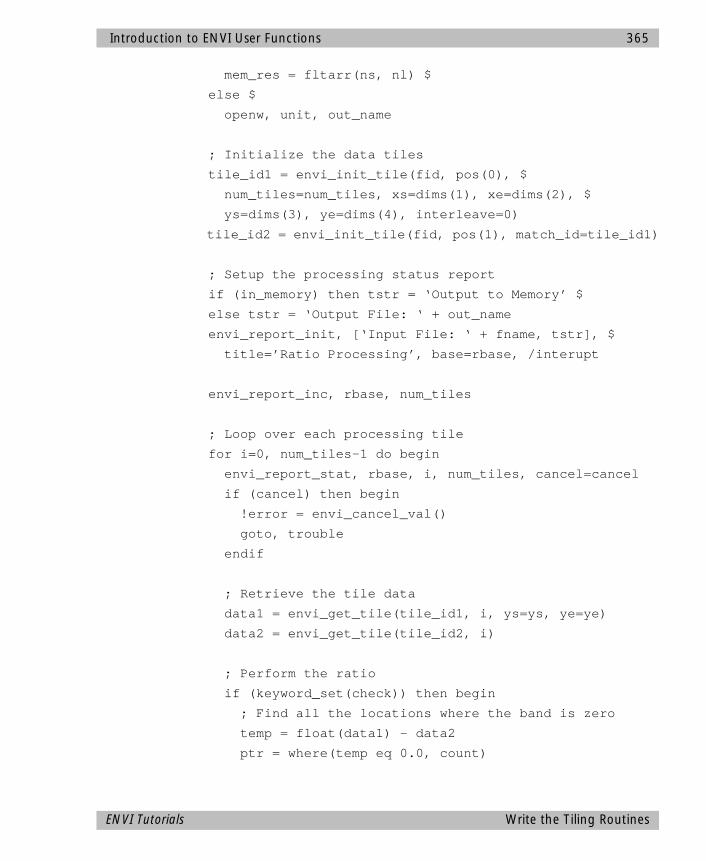
Introduction to ENVI User Functions 365
mem_res = fltarr(ns, nl) $
else $
openw, unit, out_name
; Initialize the data tiles
tile_id1 = envi_init_tile(fid, pos(0), $
num_tiles=num_tiles, xs=dims(1), xe=dims(2), $
ys=dims(3), ye=dims(4), interleave=0)
tile_id2 = envi_init_tile(fid, pos(1), match_id=tile_id1)
; Setup the processing status report
if (in_memory) then tstr = ‘Output to Memory’ $
else tstr = ‘Output File: ‘ + out_name
envi_report_init, [‘Input File: ‘ + fname, tstr], $
title=’Ratio Processing’, base=rbase, /interupt
envi_report_inc, rbase, num_tiles
; Loop over each processing tile
for i=0, num_tiles-1 do begin
envi_report_stat, rbase, i, num_tiles, cancel=cancel
if (cancel) then begin
!error = envi_cancel_val()
goto, trouble
endif
; Retrieve the tile data
data1 = envi_get_tile(tile_id1, i, ys=ys, ye=ye)
data2 = envi_get_tile(tile_id2, i)
; Perform the ratio
if (keyword_set(check)) then begin
; Find all the locations where the band is zero
temp = float(data1) - data2
ptr = where(temp eq 0.0, count)
ENVI Tutorials Write the Tiling Routines
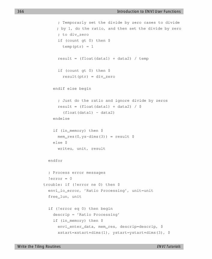
366 Introduction to ENVI User Functions
; Temporarly set the divide by zero cases to divide
; by 1, do the ratio, and then set the divide by zero
; to div_zero
if (count gt 0) then $
temp(ptr) = 1
result = (float(data1) + data2) / temp
if (count gt 0) then $
result(ptr) = div_zero
endif else begin
; Just do the ratio and ignore divide by zeros
result = (float(data1) + data2) / $
(float(data1) - data2)
endelse
if (in_memory) then $
mem_res(0,ys-dims(3)) = result $
else $
writeu, unit, result
endfor
; Process error messages
!error = 0
trouble: if (!error ne 0) then $
envi_io_error, ’Ratio Processing’, unit=unit
free_lun, unit
if (!error eq 0) then begin
descrip = ’Ratio Processing’
if (in_memory) then $
envi_enter_data, mem_res, descrip=descrip, $
xstart=xstart+dims(1), ystart=ystart+dims(3), $
Write the Tiling Routines ENVI Tutorials
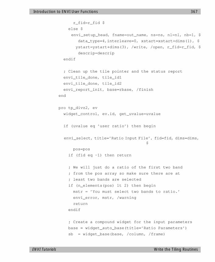
Introduction to ENVI User Functions 367
r_fid=r_fid $
else $
envi_setup_head, fname=out_name, ns=ns, nl=nl, nb=1, $
data_type=4,interleave=0, xstart=xstart+dims(1), $
ystart=ystart+dims(3), /write, /open, r_fid=r_fid, $
descrip=descrip
endif
; Clean up the tile pointer and the status report
envi_tile_done, tile_id1
envi_tile_done, tile_id2
envi_report_init, base=rbase, /finish
end
pro tp_divz2, ev
widget_control, ev.id, get_uvalue=uvalue
if (uvalue eq ’user ratio’) then begin
envi_select, title=’Ratio Input File’, fid=fid, dims=dims, $
pos=pos
if (fid eq -1) then return
; We will just do a ratio of the first two band
; from the pos array so make sure there are at
; least two bands are selected
if (n_elements(pos) lt 2) then begin
mstr = ’You must select two bands to ratio.’
envi_error, mstr, /warning
return
endif
; Create a compound widget for the input parameters
base = widget_auto_base(title=’Ratio Parameters’)
sb = widget_base(base, /column, /frame)
ENVI Tutorials Write the Tiling Routines
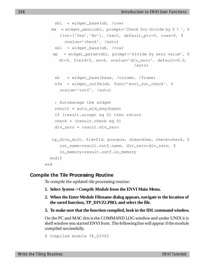
368 Introduction to ENVI User Functions
sb1 = widget_base(sb, /row)
mw = widget_menu(sb1, prompt=’Check for divide by 0 ? ’, $
list=[’Yes’,’No’], /excl, default_ptr=0, rows=0, $
uvalue=’check’, /auto)
sb1 = widget_base(sb, /row)
wp = widget_param(sb1, prompt=’Divide by zero value’, $
dt=4, field=3, xs=6, uvalue=’div_zero’, default=0.0, /auto)
sb = widget_base(base, /column, /frame)
ofw = widget_outfm(sb, func=’envi_out_check’, $
uvalue=’outf’, /auto)
; Automanage the widget
result = auto_wid_mng(base)
if (result.accept eq 0) then return
check = (result.check eq 0)
div_zero = result.div_zero
tp_divz_doit, fid=fid, pos=pos, dims=dims, check=check, $
out_name=result.outf.name, div_zero=div_zero, $
in_memory=result.outf.in_memory
endif
end
Compile the Tile Processing RoutineTo compile the updated tile processing routine:
1. Select System->Compile Module from the ENVI Main Menu.
2. When the Enter Module Filename dialog appears, navigate to the location of the saved function, TP_DIVZ2.PRO, and select the file.
3. To make sure that the function compiled, look in the IDL command window.
On the PC and MAC this is the COMMAND LOG window and under UNIX it is shell window you started ENVI from. The following line will appear if the module compiled successfully.
% Compiled module TP_DIVZ2
Write the Tiling Routines ENVI Tutorials

Introduction to ENVI User Functions 369
4. Edit and fix any errors for modules that did not compile successfully.
Run the Tile Processing Routine1. Select Utilities->User Functions->User Band Ratio2.
2. When the Ratio Input File selection dialog appears, select BLDR_TM.IMG from the “Select Input File” list widget.
Note Be sure to select “Spectral Subset” and select only bands 2 and 3.
3. In the Spectral Subset dialog, click “OK”.
4. Click “OK” in the “Ratio Input File” selection dialog.
The Ratio Exercise Parameters dialog will appear and allow the selection of divide by zero checking, replacement value, and output to memory or file.
5. Select the “Yes” toggle button for the “Check for divide by 0”.
6. Enter 1.0 for the “Divide by zero value”.
7. Select the output to “File” toggle button, enter a file name and click “OK”.
The resulting image will be placed into the Available Bands List.
Display the Result
• Select the newly created band in the Available Bands list and select “Load Band” to display the image.
This image should be the same as the Band Math example for the case that checked for divide by zero values.
End the ENVI SessionThis concludes the User Function Tutorial.
• Click “Quit” or “Exit” on the ENVI Main Menu, then type exit at the IDL command prompt.
Notes on AutocompilingThe two routines created in this tutorial can be set up to autocompile for future ENVI sessions.
• To autocompile, place the two .PRO files in the save_add directory of the ENVI installation and restart ENVI. They will be compiled whenever ENVI is started.
ENVI Tutorials Write the Tiling Routines

370 Introduction to ENVI User Functions
Write the Tiling Routines ENVI Tutorials