entropy and information theory - now the knowledge … and information theory ... 11.8 a geometric...
TRANSCRIPT

Entropy and
Information Theory

ii
Entropy and
Information Theory
Robert M. GrayInformation Systems Laboratory
Electrical Engineering DepartmentStanford University
Springer-VerlagNew York

iv
This book was prepared with LATEX and reproduced by Springer-Verlagfrom camera-ready copy supplied by the author.
c©1990 by Springer Verlag

v
to Tim, Lori, Julia, Peter,Gus, Amy Elizabeth, and Alice
and in memory of Tino

vi
Contents
Prologue xi
1 Information Sources 11.1 Introduction . . . . . . . . . . . . . . . . . . . . . . . . . . . . . . 11.2 Probability Spaces and Random Variables . . . . . . . . . . . . . 11.3 Random Processes and Dynamical Systems . . . . . . . . . . . . 51.4 Distributions . . . . . . . . . . . . . . . . . . . . . . . . . . . . . 61.5 Standard Alphabets . . . . . . . . . . . . . . . . . . . . . . . . . 101.6 Expectation . . . . . . . . . . . . . . . . . . . . . . . . . . . . . . 111.7 Asymptotic Mean Stationarity . . . . . . . . . . . . . . . . . . . 141.8 Ergodic Properties . . . . . . . . . . . . . . . . . . . . . . . . . . 15
2 Entropy and Information 172.1 Introduction . . . . . . . . . . . . . . . . . . . . . . . . . . . . . . 172.2 Entropy and Entropy Rate . . . . . . . . . . . . . . . . . . . . . 172.3 Basic Properties of Entropy . . . . . . . . . . . . . . . . . . . . . 202.4 Entropy Rate . . . . . . . . . . . . . . . . . . . . . . . . . . . . . 312.5 Conditional Entropy and Information . . . . . . . . . . . . . . . 352.6 Entropy Rate Revisited . . . . . . . . . . . . . . . . . . . . . . . 412.7 Relative Entropy Densities . . . . . . . . . . . . . . . . . . . . . . 44
3 The Entropy Ergodic Theorem 473.1 Introduction . . . . . . . . . . . . . . . . . . . . . . . . . . . . . . 473.2 Stationary Ergodic Sources . . . . . . . . . . . . . . . . . . . . . 503.3 Stationary Nonergodic Sources . . . . . . . . . . . . . . . . . . . 563.4 AMS Sources . . . . . . . . . . . . . . . . . . . . . . . . . . . . . 593.5 The Asymptotic Equipartition Property . . . . . . . . . . . . . . 63
4 Information Rates I 654.1 Introduction . . . . . . . . . . . . . . . . . . . . . . . . . . . . . . 654.2 Stationary Codes and Approximation . . . . . . . . . . . . . . . 654.3 Information Rate of Finite Alphabet Processes . . . . . . . . . . 73
vii
viii CONTENTS
5 Relative Entropy 775.1 Introduction . . . . . . . . . . . . . . . . . . . . . . . . . . . . . . 775.2 Divergence . . . . . . . . . . . . . . . . . . . . . . . . . . . . . . 775.3 Conditional Relative Entropy . . . . . . . . . . . . . . . . . . . . 925.4 Limiting Entropy Densities . . . . . . . . . . . . . . . . . . . . . 1045.5 Information for General Alphabets . . . . . . . . . . . . . . . . . 1065.6 Some Convergence Results . . . . . . . . . . . . . . . . . . . . . . 116
6 Information Rates II 1196.1 Introduction . . . . . . . . . . . . . . . . . . . . . . . . . . . . . . 1196.2 Information Rates for General Alphabets . . . . . . . . . . . . . 1196.3 A Mean Ergodic Theorem for Densities . . . . . . . . . . . . . . 1226.4 Information Rates of Stationary Processes . . . . . . . . . . . . . 124
7 Relative Entropy Rates 1317.1 Introduction . . . . . . . . . . . . . . . . . . . . . . . . . . . . . . 1317.2 Relative Entropy Densities and Rates . . . . . . . . . . . . . . . 1317.3 Markov Dominating Measures . . . . . . . . . . . . . . . . . . . . 1347.4 Stationary Processes . . . . . . . . . . . . . . . . . . . . . . . . . 1377.5 Mean Ergodic Theorems . . . . . . . . . . . . . . . . . . . . . . . 140
8 Ergodic Theorems for Densities 1458.1 Introduction . . . . . . . . . . . . . . . . . . . . . . . . . . . . . . 1458.2 Stationary Ergodic Sources . . . . . . . . . . . . . . . . . . . . . 1458.3 Stationary Nonergodic Sources . . . . . . . . . . . . . . . . . . . 1508.4 AMS Sources . . . . . . . . . . . . . . . . . . . . . . . . . . . . . 1538.5 Ergodic Theorems for Information Densities. . . . . . . . . . . . 156
9 Channels and Codes 1599.1 Introduction . . . . . . . . . . . . . . . . . . . . . . . . . . . . . . 1599.2 Channels . . . . . . . . . . . . . . . . . . . . . . . . . . . . . . . 1609.3 Stationarity Properties of Channels . . . . . . . . . . . . . . . . . 1629.4 Examples of Channels . . . . . . . . . . . . . . . . . . . . . . . . 1659.5 The Rohlin-Kakutani Theorem . . . . . . . . . . . . . . . . . . . 185
10 Distortion 19110.1 Introduction . . . . . . . . . . . . . . . . . . . . . . . . . . . . . . 19110.2 Distortion and Fidelity Criteria . . . . . . . . . . . . . . . . . . . 19110.3 Performance . . . . . . . . . . . . . . . . . . . . . . . . . . . . . . 19310.4 The rho-bar distortion . . . . . . . . . . . . . . . . . . . . . . . . 19510.5 d-bar Continuous Channels . . . . . . . . . . . . . . . . . . . . . 19710.6 The Distortion-Rate Function . . . . . . . . . . . . . . . . . . . . 201
CONTENTS ix
11 Source Coding Theorems 21111.1 Source Coding and Channel Coding . . . . . . . . . . . . . . . . 21111.2 Block Source Codes for AMS Sources . . . . . . . . . . . . . . . . 21111.3 Block Coding Stationary Sources . . . . . . . . . . . . . . . . . . 22111.4 Block Coding AMS Ergodic Sources . . . . . . . . . . . . . . . . 22211.5 Subadditive Fidelity Criteria . . . . . . . . . . . . . . . . . . . . 22811.6 Asynchronous Block Codes . . . . . . . . . . . . . . . . . . . . . 23011.7 Sliding Block Source Codes . . . . . . . . . . . . . . . . . . . . . 23211.8 A Geometric Interpretation of OPTA’s . . . . . . . . . . . . . . . 241
12 Coding for noisy channels 24312.1 Noisy Channels . . . . . . . . . . . . . . . . . . . . . . . . . . . . 24312.2 Feinstein’s Lemma . . . . . . . . . . . . . . . . . . . . . . . . . . 24412.3 Feinstein’s Theorem . . . . . . . . . . . . . . . . . . . . . . . . . 24712.4 Channel Capacity . . . . . . . . . . . . . . . . . . . . . . . . . . . 24912.5 Robust Block Codes . . . . . . . . . . . . . . . . . . . . . . . . . 25412.6 Block Coding Theorems for Noisy Channels . . . . . . . . . . . . 25712.7 Joint Source and Channel Block Codes . . . . . . . . . . . . . . . 25812.8 Synchronizing Block Channel Codes . . . . . . . . . . . . . . . . 26112.9 Sliding Block Source and Channel Coding . . . . . . . . . . . . . 265
Bibliography 275
Index 284

x CONTENTS
Prologue
This book is devoted to the theory of probabilistic information measures andtheir application to coding theorems for information sources and noisy chan-nels. The eventual goal is a general development of Shannon’s mathematicaltheory of communication, but much of the space is devoted to the tools andmethods required to prove the Shannon coding theorems. These tools form anarea common to ergodic theory and information theory and comprise severalquantitative notions of the information in random variables, random processes,and dynamical systems. Examples are entropy, mutual information, conditionalentropy, conditional information, and discrimination or relative entropy, alongwith the limiting normalized versions of these quantities such as entropy rateand information rate. Much of the book is concerned with their properties, es-pecially the long term asymptotic behavior of sample information and expectedinformation.
The book has been strongly influenced by M. S. Pinsker’s classic Informationand Information Stability of Random Variables and Processes and by the seminalwork of A. N. Kolmogorov, I. M. Gelfand, A. M. Yaglom, and R. L. Dobrushin oninformation measures for abstract alphabets and their convergence properties.Many of the results herein are extensions of their generalizations of Shannon’soriginal results. The mathematical models of this treatment are more generalthan traditional treatments in that nonstationary and nonergodic informationprocesses are treated. The models are somewhat less general than those of theSoviet school of information theory in the sense that standard alphabets ratherthan completely abstract alphabets are considered. This restriction, however,permits many stronger results as well as the extension to nonergodic processes.In addition, the assumption of standard spaces simplifies many proofs and suchspaces include as examples virtually all examples of engineering interest.
The information convergence results are combined with ergodic theoremsto prove general Shannon coding theorems for sources and channels. The re-sults are not the most general known and the converses are not the strongestavailable, but they are sufficently general to cover most systems encounteredin applications and they provide an introduction to recent extensions requiringsignificant additional mathematical machinery. Several of the generalizationshave not previously been treated in book form. Examples of novel topics for aninformation theory text include asymptotic mean stationary sources, one-sidedsources as well as two-sided sources, nonergodic sources, d-continuous channels,
xi
xii PROLOGUE
and sliding block codes. Another novel aspect is the use of recent proofs ofgeneral Shannon-McMillan-Breiman theorems which do not use martingale the-ory: A coding proof of Ornstein and Weiss [117] is used to prove the almosteverywhere convergence of sample entropy for discrete alphabet processes anda variation on the sandwich approach of Algoet and Cover [7] is used to provethe convergence of relative entropy densities for general standard alphabet pro-cesses. Both results are proved for asymptotically mean stationary processeswhich need not be ergodic.
This material can be considered as a sequel to my book Probability, RandomProcesses, and Ergodic Properties [51] wherein the prerequisite results on prob-ability, standard spaces, and ordinary ergodic properties may be found. Thisbook is self contained with the exception of common (and a few less common)results which may be found in the first book.
It is my hope that the book will interest engineers in some of the mathemat-ical aspects and general models of the theory and mathematicians in some ofthe important engineering applications of performance bounds and code designfor communication systems.
Information theory or the mathematical theory of communication has twoprimary goals: The first is the development of the fundamental theoretical lim-its on the achievable performance when communicating a given informationsource over a given communications channel using coding schemes from withina prescribed class. The second goal is the development of coding schemes thatprovide performance that is reasonably good in comparison with the optimalperformance given by the theory. Information theory was born in a surpris-ingly rich state in the classic papers of Claude E. Shannon [129] [130] whichcontained the basic results for simple memoryless sources and channels and in-troduced more general communication systems models, including finite statesources and channels. The key tools used to prove the original results and manyof those that followed were special cases of the ergodic theorem and a new vari-ation of the ergodic theorem which considered sample averages of a measure ofthe entropy or self information in a process.
Information theory can be viewed as simply a branch of applied probabilitytheory. Because of its dependence on ergodic theorems, however, it can also beviewed as a branch of ergodic theory, the theory of invariant transformationsand transformations related to invariant transformations. In order to developthe ergodic theory example of principal interest to information theory, supposethat one has a random process, which for the moment we consider as a sam-ple space or ensemble of possible output sequences together with a probabilitymeasure on events composed of collections of such sequences. The shift is thetransformation on this space of sequences that takes a sequence and produces anew sequence by shifting the first sequence a single time unit to the left. In otherwords, the shift transformation is a mathematical model for the effect of timeon a data sequence. If the probability of any sequence event is unchanged byshifting the event, that is, by shifting all of the sequences in the event, then theshift transformation is said to be invariant and the random process is said to be
PROLOGUE xiii
stationary. Thus the theory of stationary random processes can be considered asa subset of ergodic theory. Transformations that are not actually invariant (ran-dom processes which are not actually stationary) can be considered using similartechniques by studying transformations which are almost invariant, which areinvariant in an asymptotic sense, or which are dominated or asymptoticallydominated in some sense by an invariant transformation. This generality canbe important as many real processes are not well modeled as being stationary.Examples are processes with transients, processes that have been parsed intoblocks and coded, processes that have been encoded using variable-length codesor finite state codes and channels with arbitrary starting states.
Ergodic theory was originally developed for the study of statistical mechanicsas a means of quantifying the trajectories of physical or dynamical systems.Hence, in the language of random processes, the early focus was on ergodictheorems: theorems relating the time or sample average behavior of a randomprocess to its ensemble or expected behavior. The work of Hoph [65], vonNeumann [146] and others culminated in the pointwise or almost everywhereergodic theorem of Birkhoff [16].
In the 1940’s and 1950’s Shannon made use of the ergodic theorem in thesimple special case of memoryless processes to characterize the optimal perfor-mance theoretically achievable when communicating information sources overconstrained random media called channels. The ergodic theorem was appliedin a direct fashion to study the asymptotic behavior of error frequency andtime average distortion in a communication system, but a new variation wasintroduced by defining a mathematical measure of the entropy or informationin a random process and characterizing its asymptotic behavior. These resultsare known as coding theorems. Results describing performance that is actuallyachievable, at least in the limit of unbounded complexity and time, are known aspositive coding theorems. Results providing unbeatable bounds on performanceare known as converse coding theorems or negative coding theorems. When thesame quantity is given by both positive and negative coding theorems, one hasexactly the optimal performance theoretically achievable by the given commu-nication systems model.
While mathematical notions of information had existed before, it was Shan-non who coupled the notion with the ergodic theorem and an ingenious ideaknown as “random coding” in order to develop the coding theorems and tothereby give operational significance to such information measures. The name“random coding” is a bit misleading since it refers to the random selection ofa deterministic code and not a coding system that operates in a random orstochastic manner. The basic approach to proving positive coding theoremswas to analyze the average performance over a random selection of codes. Ifthe average is good, then there must be at least one code in the ensemble ofcodes with performance as good as the average. The ergodic theorem is cru-cial to this argument for determining such average behavior. Unfortunately,such proofs promise the existence of good codes but give little insight into theirconstruction.
Shannon’s original work focused on memoryless sources whose probability
xiv PROLOGUE
distribution did not change with time and whose outputs were drawn from a fi-nite alphabet or the real line. In this simple case the well-known ergodic theoremimmediately provided the required result concerning the asymptotic behavior ofinformation. He observed that the basic ideas extended in a relatively straight-forward manner to more complicated Markov sources. Even this generalization,however, was a far cry from the general stationary sources considered in theergodic theorem.
To continue the story requires a few additional words about measures ofinformation. Shannon really made use of two different but related measures.The first was entropy, an idea inherited from thermodynamics and previouslyproposed as a measure of the information in a random signal by Hartley [64].Shannon defined the entropy of a discrete time discrete alphabet random pro-cess Xn, which we denote by H(X) while deferring its definition, and maderigorous the idea that the the entropy of a process is the amount of informa-tion in the process. He did this by proving a coding theorem showing thatif one wishes to code the given process into a sequence of binary symbols sothat a receiver viewing the binary sequence can reconstruct the original processperfectly (or nearly so), then one needs at least H(X) binary symbols or bits(converse theorem) and one can accomplish the task with very close to H(X)bits (positive theorem). This coding theorem is known as the noiseless sourcecoding theorem.
The second notion of information used by Shannon was mutual information.Entropy is really a notion of self information–the information provided by arandom process about itself. Mutual information is a measure of the informationcontained in one process about another process. While entropy is sufficient tostudy the reproduction of a single process through a noiseless environment, moreoften one has two or more distinct random processes, e.g., one random processrepresenting an information source and another representing the output of acommunication medium wherein the coded source has been corrupted by anotherrandom process called noise. In such cases observations are made on one processin order to make decisions on another. Suppose that Xn, Yn is a randomprocess with a discrete alphabet, that is, taking on values in a discrete set. Thecoordinate random processes Xn and Yn might correspond, for example,to the input and output of a communication system. Shannon introduced thenotion of the average mutual information between the two processes:
I(X,Y ) = H(X) + H(Y ) − H(X,Y ), (1)
the sum of the two self entropies minus the entropy of the pair. This proved tobe the relevant quantity in coding theorems involving more than one distinctrandom process: the channel coding theorem describing reliable communicationthrough a noisy channel, and the general source coding theorem describing thecoding of a source for a user subject to a fidelity criterion. The first theoremfocuses on error detection and correction and the second on analog-to-digitalconversion and data compression. Special cases of both of these coding theoremswere given in Shannon’s original work.
PROLOGUE xv
Average mutual information can also be defined in terms of conditional en-tropy (or equivocation) H(X|Y ) = H(X,Y ) − H(Y ) and hence
I(X,Y ) = H(X) − H(X|Y ) = H(Y ) − H(X|Y ). (2)
In this form the mutual information can be interpreted as the information con-tained in one process minus the information contained in the process when theother process is known. While elementary texts on information theory aboundwith such intuitive descriptions of information measures, we will minimize suchdiscussion because of the potential pitfall of using the interpretations to applysuch measures to problems where they are not appropriate. ( See, e.g., P. Elias’“Information theory, photosynthesis, and religion” in his “Two famous papers”[36].) Information measures are important because coding theorems exist im-buing them with operational significance and not because of intuitively pleasingaspects of their definitions.
We focus on the definition (1) of mutual information since it does not requireany explanation of what conditional entropy means and since it has a moresymmetric form than the conditional definitions. It turns out that H(X,X) =H(X) (the entropy of a random variable is not changed by repeating it) andhence from (1)
I(X,X) = H(X) (3)
so that entropy can be considered as a special case of average mutual informa-tion.
To return to the story, Shannon’s work spawned the new field of informationtheory and also had a profound effect on the older field of ergodic theory.
Information theorists, both mathematicians and engineers, extended Shan-non’s basic approach to ever more general models of information sources, codingstructures, and performance measures. The fundamental ergodic theorem forentropy was extended to the same generality as the ordinary ergodic theorems byMcMillan [103] and Breiman [19] and the result is now known as the Shannon-McMillan-Breiman theorem. (Other names are the asymptotic equipartitiontheorem or AEP, the ergodic theorem of information theory, and the entropytheorem.) A variety of detailed proofs of the basic coding theorems and strongerversions of the theorems for memoryless, Markov, and other special cases of ran-dom processes were developed, notable examples being the work of Feinstein [38][39] and Wolfowitz (see, e.g., Wolfowitz [151].) The ideas of measures of infor-mation, channels, codes, and communications systems were rigorously extendedto more general random processes with abstract alphabets and discrete andcontinuous time by Khinchine [72], [73] and by Kolmogorov and his colleagues,especially Gelfand, Yaglom, Dobrushin, and Pinsker [45], [90], [87], [32], [125].(See, for example, “Kolmogorov’s contributions to information theory and algo-rithmic complexity” [23].) In almost all of the early Soviet work, it was averagemutual information that played the fundamental role. It was the more naturalquantity when more than one process were being considered. In addition, thenotion of entropy was not useful when dealing with processes with continuousalphabets since it is virtually always infinite in such cases. A generalization of
xvi PROLOGUE
the idea of entropy called discrimination was developed by Kullback (see, e.g.,Kullback [92]) and was further studied by the Soviet school. This form of infor-mation measure is now more commonly referred to as relative entropy or crossentropy (or Kullback-Leibler number) and it is better interpreted as a measureof similarity between probability distributions than as a measure of informationbetween random variables. Many results for mutual information and entropycan be viewed as special cases of results for relative entropy and the formula forrelative entropy arises naturally in some proofs.
It is the mathematical aspects of information theory and hence the descen-dants of the above results that are the focus of this book, but the developmentsin the engineering community have had as significant an impact on the founda-tions of information theory as they have had on applications. Simpler proofs ofthe basic coding theorems were developed for special cases and, as a natural off-shoot, the rate of convergence to the optimal performance bounds characterizedin a variety of important cases. See, e.g., the texts by Gallager [43], Berger [11],and Csiszar and Korner [26]. Numerous practicable coding techniques were de-veloped which provided performance reasonably close to the optimum in manycases: from the simple linear error correcting and detecting codes of Slepian[137] to the huge variety of algebraic codes currently being implemented (see,e.g., [13], [148],[95], [97], [18]) and the various forms of convolutional, tree, andtrellis codes for error correction and data compression (see, e.g., [145], [69]).Clustering techniques have been used to develop good nonlinear codes (called“vector quantizers”) for data compression applications such as speech and imagecoding [49], [46], [99], [69], [118]. These clustering and trellis search techniqueshave been combined to form single codes that combine the data compressionand reliable communication operations into a single coding system [8].
The engineering side of information theory through the middle 1970’s hasbeen well chronicled by two IEEE collections: Key Papers in the Developmentof Information Theory, edited by D. Slepian [138], and Key Papers in the Devel-opment of Coding Theory, edited by E. Berlekamp [14]. In addition there havebeen several survey papers describing the history of information theory duringeach decade of its existence published in the IEEE Transactions on InformationTheory.
The influence on ergodic theory of Shannon’s work was equally great but ina different direction. After the development of quite general ergodic theorems,one of the principal issues of ergodic theory was the isomorphism problem, thecharacterization of conditions under which two dynamical systems are really thesame in the sense that each could be obtained from the other in an invertibleway by coding. Here, however, the coding was not of the variety consideredby Shannon: Shannon considered block codes, codes that parsed the data intononoverlapping blocks or windows of finite length and separately mapped eachinput block into an output block. The more natural construct in ergodic theorycan be called a sliding block code: Here the encoder views a block of possiblyinfinite length and produces a single symbol of the output sequence using somemapping (or code or filter). The input sequence is then shifted one time unit tothe left, and the same mapping applied to produce the next output symbol, and
PROLOGUE xvii
so on. This is a smoother operation than the block coding structure since theoutputs are produced based on overlapping windows of data instead of on a com-pletely different set of data each time. Unlike the Shannon codes, these codeswill produce stationary output processes if given stationary input processes. Itshould be mentioned that examples of such sliding block codes often occurredin the information theory literature: time-invariant convolutional codes or, sim-ply, time-invariant linear filters are sliding block codes. It is perhaps odd thatvirtually all of the theory for such codes in the information theory literaturewas developed by effectively considering the sliding block codes as very longblock codes. Recently sliding block codes have proved a useful structure for thedesign of noiseless codes for constrained alphabet channels such as magneticrecording devices, and techniques from symbolic dynamics have been applied tothe design of such codes. See, for example [3], [100].
Shannon’s noiseless source coding theorem suggested a solution to the iso-morphism problem: If we assume for the moment that one of the two processesis binary, then perfect coding of a process into a binary process and back intothe original process requires that the original process and the binary processhave the same entropy. Thus a natural conjecture is that two processes are iso-morphic if and only if they have the same entropy. A major difficulty was thefact that two different kinds of coding were being considered: stationary slidingblock codes with zero error by the ergodic theorists and either fixed length blockcodes with small error or variable length (and hence nonstationary) block codeswith zero error by the Shannon theorists. While it was plausible that the formercodes might be developed as some sort of limit of the latter, this proved to bean extremely difficult problem. It was Kolmogorov [88], [89] who first reasonedalong these lines and proved that in fact equal entropy (appropriately defined)was a necessary condition for isomorphism.
Kolmogorov’s seminal work initiated a new branch of ergodic theory devotedto the study of entropy of dynamical systems and its application to the isomor-phism problem. Most of the original work was done by Soviet mathematicians;notable papers are those by Sinai [134] [135] (in ergodic theory entropy is alsoknown as the Kolmogorov-Sinai invariant), Pinsker [125], and Rohlin and Sinai[127]. An actual construction of a perfectly noiseless sliding block code for aspecial case was provided by Meshalkin [104]. While much insight was gainedinto the behavior of entropy and progress was made on several simplified ver-sions of the isomorphism problem, it was several years before Ornstein [114]proved a result that has since come to be known as the Kolmogorov-Ornsteinisomorphism theorem.
Ornstein showed that if one focused on a class of random processes whichwe shall call B-processes, then two processes are indeed isomorphic if and onlyif they have the same entropy. B-processes have several equivalent definitions,perhaps the simplest is that they are processes which can be obtained by encod-ing a memoryless process using a sliding block code. This class remains the mostgeneral class known for which the isomorphism conjecture holds. In the courseof his proof, Ornstein developed intricate connections between block coding andsliding block coding. He used Shannonlike techniques on the block codes, then
xviii PROLOGUE
imbedded the block codes into sliding block codes, and then used the stationarystructure of the sliding block codes to advantage in limiting arguments to obtainthe required zero error codes. Several other useful techniques and results wereintroduced in the proof: notions of the distance between processes and relationsbetween the goodness of approximation and the difference of entropy. Ornsteinexpanded these results into a book [116] and gave a tutorial discussion in thepremier issue of the Annals of Probability [115]. Several correspondence itemsby other ergodic theorists discussing the paper accompanied the article.
The origins of this book lie in the tools developed by Ornstein for the proofof the isomorphism theorem rather than with the result itself. During the early1970’s I first become interested in ergodic theory because of joint work with LeeD. Davisson on source coding theorems for stationary nonergodic processes. Theergodic decomposition theorem discussed in Ornstein [115] provided a neededmissing link and led to an intense campaign on my part to learn the funda-mentals of ergodic theory and perhaps find other useful tools. This effort wasgreatly eased by Paul Shields’ book The Theory of Bernoulli Shifts [131] and bydiscussions with Paul on topics in both ergodic theory and information theory.This in turn led to a variety of other applications of ergodic theoretic techniquesand results to information theory, mostly in the area of source coding theory:proving source coding theorems for sliding block codes and using process dis-tance measures to prove universal source coding theorems and to provide newcharacterizations of Shannon distortion-rate functions. The work was done withDave Neuhoff, like me then an apprentice ergodic theorist, and Paul Shields.
With the departure of Dave and Paul from Stanford, my increasing inter-est led me to discussions with Don Ornstein on possible applications of histechniques to channel coding problems. The interchange often consisted of mydescribing a problem, his generation of possible avenues of solution, and thenmy going off to work for a few weeks to understand his suggestions and workthem through.
One problem resisted our best efforts–how to synchronize block codes overchannels with memory, a prerequisite for constructing sliding block codes forsuch channels. In 1975 I had the good fortune to meet and talk with Roland Do-brushin at the 1975 IEEE/USSR Workshop on Information Theory in Moscow.He observed that some of his techniques for handling synchronization in memo-ryless channels should immediately generalize to our case and therefore shouldprovide the missing link. The key elements were all there, but it took sevenyears for the paper by Ornstein, Dobrushin and me to evolve and appear [59].
Early in the course of the channel coding paper, I decided that having thesolution to the sliding block channel coding result in sight was sufficient excuseto write a book on the overlap of ergodic theory and information theory. Theintent was to develop the tools of ergodic theory of potential use to informationtheory and to demonstrate their use by proving Shannon coding theorems forthe most general known information sources, channels, and code structures.Progress on the book was disappointingly slow, however, for a number of reasons.As delays mounted, I saw many of the general coding theorems extended andimproved by others (often by J. C. Kieffer) and new applications of ergodic
PROLOGUE xix
theory to information theory developed, such as the channel modeling workof Neuhoff and Shields [110], [113], [112], [111] and design methods for slidingblock codes for input restricted noiseless channels by Adler, Coppersmith, andHasner [3] and Marcus [100]. Although I continued to work in some aspects ofthe area, especially with nonstationary and nonergodic processes and processeswith standard alphabets, the area remained for me a relatively minor one andI had little time to write. Work and writing came in bursts during sabbaticalsand occasional advanced topic seminars. I abandoned the idea of providing themost general possible coding theorems and decided instead to settle for codingtheorems that were sufficiently general to cover most applications and whichpossessed proofs I liked and could understand. The mantle of the most generaltheorems will go to a book in progress by J.C. Kieffer [85]. That book sharesmany topics with this one, but the approaches and viewpoints and many of theresults treated are quite different. At the risk of generalizing, the books willreflect our differing backgrounds: mine as an engineer by training and a would-be mathematician, and his as a mathematician by training migrating to anengineering school. The proofs of the principal results often differ in significantways and the two books contain a variety of different minor results developedas tools along the way. This book is perhaps more “old fashioned” in thatthe proofs often retain the spirit of the original “classical” proofs, while Kiefferhas developed a variety of new and powerful techniques to obtain the mostgeneral known results. I have also taken more detours along the way in orderto catalog various properties of entropy and other information measures that Ifound interesting in their own right, even though they were not always necessaryfor proving the coding theorems. Only one third of this book is actually devotedto Shannon source and channel coding theorems; the remainder can be viewedas a monograph on information measures and their properties, especially theirergodic properties.
Because of delays in the original project, the book was split into two smallerbooks and the first, Probability, Random Processes, and Ergodic Properties,was published by Springer-Verlag in 1988 [50]. It treats advanced probabilityand random processes with an emphasis on processes with standard alphabets,on nonergodic and nonstationary processes, and on necessary and sufficientconditions for the convergence of long term sample averages. Asymptoticallymean stationary sources and the ergodic decomposition are there treated indepth and recent simplified proofs of the ergodic theorem due to Ornstein andWeiss [117] and others were incorporated. That book provides the backgroundmaterial and introduction to this book, the split naturally falling before theintroduction of entropy. The first chapter of this book reviews some of the basicnotation of the first one in information theoretic terms, but results are oftensimply quoted as needed from the first book without any attempt to derivethem. The two books together are self-contained in that all supporting resultsfrom probability theory and ergodic theory needed here may be found in thefirst book. This book is self-contained so far as its information theory content,but it should be considered as an advanced text on the subject and not as an
xx PROLOGUE
introductory treatise to the reader only wishing an intuitive overview.Here the Shannon-McMillan-Breiman theorem is proved using the coding
approach of Ornstein and Weiss [117] (see also Shield’s tutorial paper [132])and hence the treatments of ordinary ergodic theorems in the first book and theergodic theorems for information measures in this book are consistent. The ex-tension of the Shannon-McMillan-Breiman theorem to densities is proved usingthe “sandwich” approach of Algoet and Cover [7], which depends strongly onthe usual pointwise or Birkhoff ergodic theorem: sample entropy is asymptot-ically sandwiched between two functions whose limits can be determined fromthe ergodic theorem. These results are the most general yet published in bookform and differ from traditional developments in that martingale theory is notrequired in the proofs.
A few words are in order regarding topics that are not contained in thisbook. I have not included multiuser information theory for two reasons: First,after including the material that I wanted most, there was no room left. Second,my experience in the area is slight and I believe this topic can be better handledby others. Results as general as the single user systems described here have notyet been developed. Good surveys of the multiuser area may be found in ElGamal and Cover [44], van der Meulen [142], and Berger [12].
Traditional noiseless coding theorems and actual codes such as the Huff-man codes are not considered in depth because quite good treatments exist inthe literature, e.g., [43], [1], [102]. The corresponding ergodic theory result–the Kolmogorov-Ornstein isomorphism theorem–is also not proved, because itsproof is difficult and the result is not needed for the Shannon coding theorems.Many techniques used in its proof, however, are used here for similar and otherpurposes.
The actual computation of channel capacity and distortion rate functionshas not been included because existing treatments [43], [17], [11], [52] are quiteadequate.
This book does not treat code design techniques. Algebraic coding is welldeveloped in existing texts on the subject [13], [148], [95], [18]. Allen Gersho andI are currently writing a book on the theory and design of nonlinear coding tech-niques such as vector quantizers and trellis codes for analog-to-digital conversionand for source coding (data compression) and combined source and channel cod-ing applications [47]. A less mathematical treatment of rate-distortion theoryalong with other source coding topics not treated here (including asymptotic,or high rate, quantization theory and uniform quantizer noise theory) may befound in my book [52].
Universal codes, codes which work well for an unknown source, and variablerate codes, codes producing a variable number of bits for each input vector, arenot considered. The interested reader is referred to [109] [96] [77] [78] [28] andthe references therein.
A recent active research area that has made good use of the ideas of rel-ative entropy to characterize exponential growth is that of large deviationstheory[143][31]. These techniques have been used to provide new proofs of the
PROLOGUE xxi
basic source coding theorems[22]. These topics are not treated here.Lastly, J. C. Kieffer has recently developed a powerful new ergodic theorem
that can be used to prove both traditional ergodic theorems and the extendedShannon-McMillan-Brieman theorem [83]. He has used this theorem to provenew strong (almost everywhere) versions of the souce coding theorem and itsconverse, that is, results showing that sample average distortion is with proba-bility one no smaller than the distortion-rate function and that there exist codeswith sample average distortion arbitrarily close to the distortion-rate function[84] [82]. These results should have a profound impact on the future develop-ment of the theoretical tools and results of information theory. Their imminentpublication provide a strong motivation for the completion of this monograph,which is devoted to the traditional methods. Tradition has its place, however,and the methods and results treated here should retain much of their role at thecore of the theory of entropy and information. It is hoped that this collectionof topics and methods will find a niche in the literature.
19 November 2000 Revision The original edition went out of print in2000. Hence I took the opportunity to fix more typos which have been broughtto my attention (thanks in particular to Yariv Ephraim) and to prepare the bookfor Web posting. This is done with the permission of the original publisher andcopyright-holder, Springer-Verlag. I hope someday to do some more seriousrevising, but for the moment I am content to fix the known errors and make themanuscript available.
xxii PROLOGUE
Acknowledgments
The research in information theory that yielded many of the results and someof the new proofs for old results in this book was supported by the NationalScience Foundation. Portions of the research and much of the early writing weresupported by a fellowship from the John Simon Guggenheim Memorial Founda-tion. The book was originally written using the eqn and troff utilities on severalUNIX systems and was subsequently translated into LATEX on both UNIX andApple Macintosh systems. All of these computer systems were supported bythe Industrial Affiliates Program of the Stanford University Information Sys-tems Laboratory. Much helpful advice on the mysteries of LATEX was providedby Richard Roy and Marc Goldburg.
The book benefited greatly from comments from numerous students andcolleagues over many years; most notably Paul Shields, Paul Algoet, EnderAyanoglu, Lee Davisson, John Kieffer, Dave Neuhoff, Don Ornstein, Bob Fontana,Jim Dunham, Farivar Saadat, Michael Sabin, Andrew Barron, Phil Chou, TomLookabaugh, Andrew Nobel, and Bradley Dickinson.
Robert M. GrayLa Honda, California
April 1990
Chapter 1
Information Sources
1.1 Introduction
An information source or source is a mathematical model for a physical entitythat produces a succession of symbols called “outputs” in a random manner.The symbols produced may be real numbers such as voltage measurements froma transducer, binary numbers as in computer data, two dimensional intensityfields as in a sequence of images, continuous or discontinuous waveforms, andso on. The space containing all of the possible output symbols is called thealphabet of the source and a source is essentially an assignment of a probabilitymeasure to events consisting of sets of sequences of symbols from the alphabet.It is useful, however, to explicitly treat the notion of time as a transformationof sequences produced by the source. Thus in addition to the common randomprocess model we shall also consider modeling sources by dynamical systems asconsidered in ergodic theory.
The material in this chapter is a distillation of [50] and is intended to estab-lish notation.
1.2 Probability Spaces and Random Variables
A measurable space (Ω,B) is a pair consisting of a sample space Ω together witha σ-field B of subsets of Ω (also called the event space). A σ-field or σ-algebraB is a nonempty collection of subsets of Ω with the following properties:
Ω ∈ B. (1.1)
If F ∈ B, then F c = ω : ω 6∈ F ∈ B. (1.2)
If Fi ∈ B; i = 1, 2, · · · , then⋃i
Fi ∈ B. (1.3)
1
2 CHAPTER 1. INFORMATION SOURCES
From de Morgan’s “laws” of elementary set theory it follows that also
∞⋂i=1
Fi = (∞⋃
i=1
F ci )c ∈ B.
An event space is a collection of subsets of a sample space (called events byvirtue of belonging to the event space) such that any countable sequence of settheoretic operations (union, intersection, complementation) on events producesother events. Note that there are two extremes: the largest possible σ-field ofΩ is the collection of all subsets of Ω (sometimes called the power set) and thesmallest possible σ-field is Ω, ∅, the entire space together with the null set∅ = Ωc (called the trivial space).
If instead of the closure under countable unions required by (1.2.3), we onlyrequire that the collection of subsets be closed under finite unions, then we saythat the collection of subsets is a field.
While the concept of a field is simpler to work with, a σ-field possesses theadditional important property that it contains all of the limits of sequences ofsets in the collection. That is, if Fn, n = 1, 2, · · · is an increasing sequence ofsets in a σ-field, that is, if Fn−1 ⊂ Fn and if F =
⋃∞n=1 Fn (in which case we
write Fn ↑ F or limn→∞ Fn = F ), then also F is contained in the σ-field. Ina similar fashion we can define decreasing sequences of sets: If Fn decreases toF in the sense that Fn+1 ⊂ Fn and F =
⋂∞n=1 Fn, then we write Fn ↓ F . If
Fn ∈ B for all n, then F ∈ B.A probability space (Ω,B, P ) is a triple consisting of a sample space Ω , a σ-
field B of subsets of Ω , and a probability measure P which assigns a real numberP (F ) to every member F of the σ-field B so that the following conditions aresatisfied:
• Nonnegativity:P (F ) ≥ 0, all F ∈ B; (1.4)
• Normalization:P (Ω) = 1; (1.5)
• Countable Additivity:
If Fi ∈ B, i = 1, 2, · · · are disjoint, then
P (∞⋃
i=1
Fi) =∞∑
i=1
P (Fi). (1.6)
A set function P satisfying only (1.2.4) and (1.2.6) but not necessarily (1.2.5)is called a measure and the triple (Ω,B, P ) is called a measure space. Since theprobability measure is defined on a σ-field, such countable unions of subsets ofΩ in the σ-field are also events in the σ-field.
A standard result of basic probability theory is that if Gn ↓ ∅ (the empty ornull set), that is, if Gn+1 ⊂ Gn for all n and
⋂∞n=1 Gn = ∅ , then we have
1.2. PROBABILITY SPACES AND RANDOM VARIABLES 3
• Continuity at ∅:lim
n→∞P (Gn) = 0. (1.7)
similarly it follows that we have
• Continuity from Below:
If Fn ↑ F, then limn→∞
P (Fn) = P (F ), (1.8)
and
• Continuity from Above:
If Fn ↓ F, then limn→∞
P (Fn) = P (F ). (1.9)
Given a measurable space (Ω,B), a collection G of members of B is said togenerate B and we write σ(G) = B if B is the smallest σ-field that contains G;that is, if a σ-field contains all of the members of G, then it must also contain allof the members of B. The following is a fundamental approximation theorem ofprobability theory. A proof may be found in Corollary 1.5.3 of [50]. The resultis most easily stated in terms of the symmetric difference ∆ defined by
F∆G ≡ (F⋂
Gc)⋂
(F c⋃
G).
Theorem 1.2.1: Given a probability space (Ω,B, P ) and a generating fieldF , that is, F is a field and B = σ(F), then given F ∈ B and ε > 0, there existsan F0 ∈ F such that P (F∆F0) ≤ ε.
Let (A,BA) denote another measurable space. A random variable or mea-surable function defined on (Ω,B) and taking values in (A,BA) is a mapping orfunction f : Ω → A with the property that
if F ∈ BA, then f−1(F ) = ω : f(ω) ∈ F ∈ B. (1.10)
The name “random variable” is commonly associated with the special case whereA is the real line and B the Borel field, the smallest σ-field containing all theintervals. Occasionally a more general sounding name such as “random object”is used for a measurable function to implicitly include random variables (A thereal line), random vectors (A a Euclidean space), and random processes (A asequence or waveform space). We will use the terms “random variable” in themore general sense.
A random variable is just a function or mapping with the property thatinverse images of “output events” determined by the random variable are eventsin the original measurable space. This simple property ensures that the outputof the random variable will inherit its own probability measure. For example,with the probability measure Pf defined by
Pf (B) = P (f−1(B)) = P (ω : f(ω) ∈ B); B ∈ BA,
4 CHAPTER 1. INFORMATION SOURCES
(A,BA, Pf ) becomes a probability space since measurability of f and elemen-tary set theory ensure that Pf is indeed a probability measure. The inducedprobability measure Pf is called the distribution of the random variable f . Themeasurable space (A,BA) or, simply, the sample space A, is called the alphabetof the random variable f . We shall occasionally also use the notation Pf−1
which is a mnemonic for the relation Pf−1(F ) = P (f−1(F )) and which is lessawkward when f itself is a function with a complicated name, e.g., ΠI→M.
If the alphabet A of a random variable f is not clear from context, then weshall refer to f as an A-valued random variable. If f is a measurable functionfrom (Ω,B) to (A,BA), we will say that f is B/BA-measurable if the σ-fieldsmight not be clear from context.
Given a probability space (Ω,B, P ), a collection of subsets G is a sub-σ-fieldif it is a σ-field and all its members are in B. A random variable f : Ω → Ais said to be measurable with respect to a sub-σ-field G if f−1(H) ∈ G for allH ∈ BA.
Given a probability space (Ω,B, P ) and a sub-σ-field G, for any event H ∈ Bthe conditional probability m(H|G) is defined as any function, say g, whichsatisfies the two properties
g is measurable with respect to G (1.11)
∫G
ghdP = m(G⋂
H); all G ∈ G. (1.12)
An important special case of conditional probability occurs when studyingthe distributions of random variables defined on an underlying probability space.Suppose that X : Ω → AX and Y : Ω → AY are two random variables definedon (Ω,B, P ) with alphabets AX and AY and σ-fields BAX
and BAY, respectively.
Let PXY denote the induced distribution on (AX × AY ,BAX× BAY
), that is,PXY (F × G) = P (X ∈ F, Y ∈ G) = P (X−1(F )
⋂Y −1(G)). Let σ(Y ) denote
the sub-σ-field of B generated by Y , that is, Y −1(BAY). Since the conditional
probability P (F |σ(Y )) is real-valued and measurable with respect to σ(Y ), itcan be written as g(Y (ω)), ω ∈ Ω, for some function g(y). (See, for example,Lemma 5.2.1 of [50].) Define P (F |y) = g(y). For a fixed F ∈ BAX
define theconditional distribution of F given Y = y by
PX|Y (F |y) = P (X−1(F )|y); y ∈ BAY.
From the properties of conditional probability,
PXY (F × G) =∫
G
PX|Y (F |y)dPY (y);F ∈ BAX, G ∈ BAY
. (1.13)
It is tempting to think that for a fixed y, the set function defined byPX|Y (F |y); F ∈ BAX
is actually a probability measure. This is not the case ingeneral. When it does hold for a conditional probability measure, the condi-tional probability measure is said to be regular. As will be emphasized later, thistext will focus on standard alphabets for which regular conditional probabilitesalways exist.
1.3. RANDOM PROCESSES AND DYNAMICAL SYSTEMS 5
1.3 Random Processes and Dynamical Systems
We now consider two mathematical models for a source: A random processand a dynamical system. The first is the familiar one in elementary courses, asource is just a random process or sequence of random variables. The secondmodel is possibly less familiar; a random process can also be constructed froman abstract dynamical system consisting of a probability space together with atransformation on the space. The two models are connected by considering atime shift to be a transformation.
A discrete time random process or for our purposes simply a random processis a sequence of random variables Xnn∈T or Xn;n ∈ T , where T is anindex set, defined on a common probability space (Ω,B, P ). We define a sourceas a random process, although we could also use the alternative definition ofa dynamical system to be introduced shortly. We usually assume that all ofthe random variables share a common alphabet, say A. The two most commonindex sets of interest are the set of all integers Z = · · · ,−2,−1, 0, 1, 2, · · ·,in which case the random process is referred to as a two-sided random process,and the set of all nonnegative integers Z+ = 0, 1, 2, · · ·, in which case therandom process is said to be one-sided. One-sided random processes will oftenprove to be far more difficult in theory, but they provide better models forphysical random processes that must be “turned on” at some time or whichhave transient behavior.
Observe that since the alphabet A is general, we could also model continuoustime random processes in the above fashion by letting A consist of a family ofwaveforms defined on an interval, e.g., the random variable Xn could in fact bea continuous time waveform X(t) for t ∈ [nT, (n + 1)T ), where T is some fixedpositive real number.
The above definition does not specify any structural properties of the indexset T . In particular, it does not exclude the possibility that T be a finite set, inwhich case “random vector” would be a better name than “random process.” Infact, the two cases of T = Z and T = Z+ will be the only important examplesfor our purposes. Nonetheless, the general notation of T will be retained inorder to avoid having to state separate results for these two cases.
An abstract dynamical system consists of a probability space (Ω,B, P ) to-gether with a measurable transformation T : Ω → Ω of Ω into itself. Measura-bility means that if F ∈ B, then also T−1F = ω : Tω ∈ F∈ B. The quadruple(Ω,B,P ,T ) is called a dynamical system in ergodic theory. The interested readercan find excellent introductions to classical ergodic theory and dynamical systemtheory in the books of Halmos [62] and Sinai [136]. More complete treatmentsmay be found in [15], [131], [124], [30], [147], [116], [42]. The term “dynamicalsystems” comes from the focus of the theory on the long term “dynamics” or“dynamical behavior” of repeated applications of the transformation T on theunderlying measure space.
An alternative to modeling a random process as a sequence or family ofrandom variables defined on a common probability space is to consider a sin-gle random variable together with a transformation defined on the underlying
6 CHAPTER 1. INFORMATION SOURCES
probability space. The outputs of the random process will then be values of therandom variable taken on transformed points in the original space. The trans-formation will usually be related to shifting in time and hence this viewpoint willfocus on the action of time itself. Suppose now that T is a measurable mappingof points of the sample space Ω into itself. It is easy to see that the cascade orcomposition of measurable functions is also measurable. Hence the transforma-tion Tn defined as T 2ω = T (Tω) and so on (Tnω = T (Tn−1ω)) is a measurablefunction for all positive integers n. If f is an A-valued random variable definedon (Ω, B), then the functions fTn : Ω → A defined by fTn(ω) = f(Tnω) forω ∈ Ω will also be random variables for all n in Z+. Thus a dynamical systemtogether with a random variable or measurable function f defines a one-sidedrandom process Xnn∈Z+ by Xn(ω) = f(Tnω). If it should be true that T isinvertible, that is, T is one-to-one and its inverse T−1 is measurable, then onecan define a two-sided random process by Xn(ω) = f(Tnω), all n in Z.
The most common dynamical system for modeling random processes is thatconsisting of a sequence space Ω containing all one- or two-sided A-valued se-quences together with the shift transformation T , that is, the transformationthat maps a sequence xn into the sequence xn+1 wherein each coordinatehas been shifted to the left by one time unit. Thus, for example, let Ω = AZ+
= all x = (x0, x1, · · ·) with xi ∈ A for all i and define T : Ω → Ω byT (x0, x1, x2, · · ·) = (x1, x2, x3, · · ·). T is called the shift or left shift transforma-tion on the one-sided sequence space. The shift for two-sided spaces is definedsimilarly.
The different models provide equivalent models for a given process: oneemphasizing the sequence of outputs and the other emphasising the action of atransformation on the underlying space in producing these outputs. In order todemonstrate in what sense the models are equivalent for given random processes,we next turn to the notion of the distribution of a random process.
1.4 Distributions
While in principle all probabilistic quantities associated with a random processcan be determined from the underlying probability space, it is often more con-venient to deal with the induced probability measures or distributions on thespace of possible outputs of the random process. In particular, this allows us tocompare different random processes without regard to the underlying probabil-ity spaces and thereby permits us to reasonably equate two random processesif their outputs have the same probabilistic structure, even if the underlyingprobability spaces are quite different.
We have already seen that each random variable Xn of the random processXn inherits a distribution because it is measurable. To describe a process,however, we need more than simply probability measures on output values ofseparate single random variables; we require probability measures on collectionsof random variables, that is, on sequences of outputs. In order to place prob-ability measures on sequences of outputs of a random process, we first must
1.4. DISTRIBUTIONS 7
construct the appropriate measurable spaces. A convenient technique for ac-complishing this is to consider product spaces, spaces for sequences formed byconcatenating spaces for individual outputs.
Let T denote any finite or infinite set of integers. In particular, T = Z(n) =0, 1, 2, · · · , n − 1, T = Z, or T = Z+. Define xT = xii∈T . For example,xZ = (· · · , x−1, x0, x1, · · ·) is a two-sided infinite sequence. When T = Z(n) weabbreviate xZ(n) to simply xn . Given alphabets Ai, i ∈ T , define the cartesianproduct space
×i∈T
Ai = all xT : xi,∈ Ai all i in T .
In most cases all of the Ai will be replicas of a single alphabet A and the aboveproduct will be denoted simply by AT . Thus, for example, Am,m+1,···,n isthe space of all possible outputs of the process from time m to time n; AZ
is the sequence space of all possible outputs of a two-sided process. We shallabbreviate the notation for the space AZ(n), the space of all n dimensionalvectors with coordinates in A, by An .
To obtain useful σ-fields of the above product spaces, we introduce the idea ofa rectangle in a product space. A rectangle in AT taking values in the coordinateσ-fields Bi, i ∈ J , is defined as any set of the form
B = xT ∈ AT : xi ∈ Bi; all i in J , (1.14)
where J is a finite subset of the index set T and Bi ∈ Bi for all i ∈ J .(Hence rectangles are sometimes referred to as finite dimensional rectangles.) Arectangle as in (1.4.1) can be written as a finite intersection of one-dimensionalrectangles as
B =⋂i∈J
xT ∈ AT : xi ∈ Bi =⋂i∈J
Xi−1(Bi) (1.15)
where here we consider Xi as the coordinate functions Xi : AT → A defined byXi(xT ) = xi.
As rectangles in AT are clearly fundamental events, they should be membersof any useful σ-field of subsets of AT . Define the product σ-field BA
T as thesmallest σ-field containing all of the rectangles, that is, the collection of sets thatcontains the clearly important class of rectangles and the minimum amount ofother stuff required to make the collection a σ-field. To be more precise, givenan index set T of integers, let RECT (Bi, i ∈ T ) denote the set of all rectanglesin AT taking coordinate values in sets in Bi, i ∈ T . We then define the productσ-field of AT by
BAT = σ(RECT (Bi, i ∈ T )). (1.16)
Consider an index set T and an A-valued random process Xnn∈T definedon an underlying probability space (Ω,B, P ). Given any index set J ⊂ T ,measurability of the individual random variables Xn implies that of the randomvectors XJ = Xn;n ∈ J . Thus the measurable space (AJ ,BA
J ) inherits aprobability measure from the underlying space through the random variables
8 CHAPTER 1. INFORMATION SOURCES
XJ . Thus in particular the measurable space (AT ,BAT ) inherits a probability
measure from the underlying probability space and thereby determines a newprobability space (AT ,BA
T , PXT ), where the induced probability measure isdefined by
PXT (F ) = P ((XT )−1(F )) = P (ω : XT (ω) ∈ F ); F ∈ BAT . (1.17)
Such probability measures induced on the outputs of random variables are re-ferred to as distributions for the random variables, exactly as in the simpler casefirst treated. When T = m,m + 1, · · · ,m + n − 1, e.g., when we are treatingXn
m = (Xn, · · · , Xm+n−1) taking values in An, the distribution is referred toas an n-dimensional or nth order distribution and it describes the behavior ofan n-dimensional random variable. If T is the entire process index set, e.g., ifT = Z for a two-sided process or T = Z+ for a one-sided process, then theinduced probability measure is defined to be the distribution of the process.Thus, for example, a probability space (Ω,B, P ) together with a doubly infi-nite sequence of random variables Xnn∈Z induces a new probability space(AZ ,BA
Z , PXZ ) and PXZ is the distribution of the process. For simplicity, letus now denote the process distribution simply by m. We shall call the proba-bility space (AT ,BA
T ,m) induced in this way by a random process Xnn∈Zthe output space or sequence space of the random process.
Since the sequence space (AT ,BAT ,m) of a random process Xnn∈Z is a
probability space, we can define random variables and hence also random pro-cesses on this space. One simple and useful such definition is that of a samplingor coordinate or projection function defined as follows: Given a product spaceAT , define the sampling functions Πn : AT → A by
Πn(xT ) = xn, xT ∈ AT ; n ∈ T . (1.18)
The sampling function is named Π since it is also a projection. Observe that thedistribution of the random process Πnn∈T defined on the probability space(AT ,BA
T ,m) is exactly the same as the distribution of the random processXnn∈T defined on the probability space (Ω,B, P ). In fact, so far they are thesame process since the Πn simply read off the values of the Xn.
What happens, however, if we no longer build the Πn on the Xn, that is, weno longer first select ω from Ω according to P , then form the sequence xT =XT (ω) = Xn(ω)n∈T , and then define Πn(xT ) = Xn(ω)? Instead we directlychoose an x in AT using the probability measure m and then view the sequenceof coordinate values. In other words, we are considering two completely separateexperiments, one described by the probability space (Ω,B, P ) and the randomvariables Xn and the other described by the probability space (AT ,BA
T ,m)and the random variables Πn. In these two separate experiments, the actualsequences selected may be completely different. Yet intuitively the processesshould be the “same” in the sense that their statistical structures are identical,that is, they have the same distribution. We make this intuition formal bydefining two processes to be equivalent if their process distributions are identical,that is, if the probability measures on the output sequence spaces are the same,
1.4. DISTRIBUTIONS 9
regardless of the functional form of the random variables of the underlyingprobability spaces. In the same way, we consider two random variables to beequivalent if their distributions are identical.
We have described above two equivalent processes or two equivalent modelsfor the same random process, one defined as a sequence of random variableson a perhaps very complicated underlying probability space, the other definedas a probability measure directly on the measurable space of possible outputsequences. The second model will be referred to as a directly given randomprocess.
Which model is “better” depends on the application. For example, a directlygiven model for a random process may focus on the random process itself and notits origin and hence may be simpler to deal with. If the random process is thencoded or measurements are taken on the random process, then it may be betterto model the encoded random process in terms of random variables defined onthe original random process and not as a directly given random process. Thismodel will then focus on the input process and the coding operation. We shalllet convenience determine the most appropriate model.
We can now describe yet another model for the above random process, thatis, another means of describing a random process with the same distribution.This time the model is in terms of a dynamical system. Given the probabilityspace (AT ,BA
T ,m), define the (left) shift transformation T : AT → AT by
T (xT ) = T (xnn∈T ) = yT = ynn∈T ,
whereyn = xn+1, n ∈ T .
Thus the nth coordinate of yT is simply the (n + 1)st coordinate of xT . (Weassume that T is closed under addition and hence if n and 1 are in T , then sois (n + 1).) If the alphabet of such a shift is not clear from context, we willoccasionally denote the shift by TA or TAT . The shift can easily be shown tobe measurable.
Consider next the dynamical system (AT ,BAT , P, T ) and the random pro-
cess formed by combining the dynamical system with the zero time samplingfunction Π0 (we assume that 0 is a member of T ). If we define Yn(x) = Π0(Tnx)for x = xT ∈ AT , or, in abbreviated form, Yn = Π0T
n, then the random pro-cess Ynn∈T is equivalent to the processes developed above. Thus we havedeveloped three different, but equivalent, means of producing the same randomprocess. Each will be seen to have its uses.
The above development shows that a dynamical system is a more fundamen-tal entity than a random process since we can always construct an equivalentmodel for a random process in terms of a dynamical system–use the directlygiven representation, shift transformation, and zero time sampling function.
The shift transformation on a sequence space introduced above is the mostimportant transformation that we shall encounter. It is not, however, the onlyimportant transformation. When dealing with transformations we will usuallyuse the notation T to reflect the fact that it is often related to the action of a
10 CHAPTER 1. INFORMATION SOURCES
simple left shift of a sequence, yet it should be kept in mind that occasionallyother operators will be considered and the theory to be developed will remainvalid, even if T is not required to be a simple time shift. For example, we willalso consider block shifts.
Most texts on ergodic theory deal with the case of an invertible transforma-tion, that is, where T is a one-to-one transformation and the inverse mappingT−1 is measurable. This is the case for the shift on AZ , the two-sided shift. It isnot the case, however, for the one-sided shift defined on AZ+ and hence we willavoid use of this assumption. We will, however, often point out in the discussionwhat simplifications or special properties arise for invertible transformations.
Since random processes are considered equivalent if their distributions arethe same, we shall adopt the notation [A,m,X] for a random process Xn;n ∈T with alphabet A and process distribution m, the index set T usually beingclear from context. We will occasionally abbreviate this to the more commonnotation [A,m], but it is often convenient to note the name of the output ran-dom variables as there may be several, e.g., a random process may have aninput X and output Y . By “the associated probability space” of a randomprocess [A,m,X] we shall mean the sequence probability space (AT ,BA
T ,m).It will often be convenient to consider the random process as a directly givenrandom process, that is, to view Xn as the coordinate functions Πn on the se-quence space AT rather than as being defined on some other abstract space.This will not always be the case, however, as often processes will be formed bycoding or communicating other random processes. Context should render suchbookkeeping details clear.
1.5 Standard Alphabets
A measurable space (A,BA) is a standard space if there exists a sequence offinite fields Fn; n = 1, 2, · · · with the following properties:
(1) Fn ⊂ Fn+1 (the fields are increasing).
(2) BA is the smallest σ-field containing all of the Fn (the Fn generate BA orBA = σ(
⋃∞n=1 Fn)).
(3) An event Gn ∈ Fn is called an atom of the field if it is nonempty and andits only subsets which are also field members are itself and the empty set.If Gn ∈ Fn; n = 1, 2, · · · are atoms and Gn+1 ⊂ Gn for all n, then
∞⋂n=1
Gn 6= ∅.
Standard spaces are important for several reasons: First, they are a general classof spaces for which two of the key results of probability hold: (1) the Kolmogorovextension theorem showing that a random process is completely described by itsfinite order distributions, and (2) the existence of regular conditional probability
1.6. EXPECTATION 11
measures. Thus, in particular, the conditional probability measure PX|Y (F |y)of (1.13) is regular if the alphabets AX and AY are standard and hence for eachfixed y ∈ AY the set function PX|Y (F |y); F ∈ BAX
is a probability measure.In this case we can interpret PX|Y (F |y) as P (X ∈ F |Y = y). Second, theergodic decomposition theorem of ergodic theory holds for such spaces. Third,the class is sufficiently general to include virtually all examples arising in ap-plications, e.g., discrete spaces, the real line, Euclidean vector spaces, Polishspaces (complete separable metric spaces), etc. The reader is referred to [50]and the references cited therein for a detailed development of these propertiesand examples of standard spaces.
Standard spaces are not the most general space for which the Kolmogorovextension theorem, the existence of conditional probability, and the ergodicdecomposition theorem hold. These results also hold for perfect spaces whichinclude standard spaces as a special case. (See, e.g., [128],[139],[126], [98].) Welimit discussion to standard spaces, however, as they are easier to characterizeand work with and they are sufficiently general to handle most cases encounteredin applications. Although standard spaces are not the most general for which therequired probability theory results hold, they are the most general for which allfinitely additive normalized measures extend to countably additive probabilitymeasures, a property which greatly eases the proof of many of the desired results.
Throughout this book we shall assume that the alphabet A of the informationsource is a standard space.
1.6 Expectation
Let (Ω,B,m) be a probability space, e.g., the probability space of a directlygiven random process with alphabet A, (AT , BA
T ,m). A real-valued randomvariable f : Ω → R will also be called a measurement since it is often formedby taking a mapping or function of some other set of more general randomvariables, e.g., the outputs of some random process which might not have real-valued outputs. Measurements made on such processes, however, will always beassumed to be real.
Suppose next we have a measurement f whose range space or alphabetf(Ω) ⊂ R of possible values is finite. Then f is called a discrete randomvariable or discrete measurement or digital measurement or, in the commonmathematical terminology, a simple function.
Given a discrete measurement f , suppose that its range space is f(Ω) =bi, i = 1, · · · , N, where the bi are distinct. Define the sets Fi = f−1(bi) =x : f(x) = bi, i = 1, · · · , N . Since f is measurable, the Fi are all membersof B. Since the bi are distinct, the Fi are disjoint. Since every input point inΩ must map into some bi, the union of the Fi equals Ω. Thus the collectionFi; i = 1, 2, · · · , N forms a partition of Ω. We have therefore shown that any
12 CHAPTER 1. INFORMATION SOURCES
discrete measurement f can be expressed in the form
f(x) =M∑i=1
bi1Fi(x), (1.19)
where bi ∈ R, the Fi ∈ B form a partition of Ω, and 1Fiis the indicator function
of Fi, i = 1, · · · ,M . Every simple function has a unique representation in thisform with distinct bi and Fi a partition.
The expectation or ensemble average or probabilistic average or mean of adiscrete measurement f : Ω → R as in (1.6.1) with respect to a probabilitymeasure m is defined by
Emf =M∑i=0
bim(Fi). (1.20)
An immediate consequence of the definition of expectation is the simple butuseful fact that for any event F in the original probability space,
Em1F = m(F ),
that is, probabilities can be found from expectations of indicator functions.Again let (Ω,B,m) be a probability space and f : Ω → R a measurement,
that is, a real-valued random variable or measurable real-valued function. Definethe sequence of quantizers qn : R → R, n = 1, 2, · · ·, as follows:
qn(r) =
n n ≤ r(k − 1)2−n (k − 1)2−n ≤ r < k2−n; k = 1, 2, · · · , n2n
−(k − 1)2−n −k2−n ≤ r < −(k − 1)2−n; k = 1, 2, · · · , n2n
−n r < −n .
We now define expectation for general measurements in two steps. If f ≥ 0,then define
Emf = limn→∞
Em(qn(f)). (1.21)
Since the qn are discrete measurements on f , the qn(f) are discrete measure-ments on Ω (qn(f)(x) = qn(f(x)) is a simple function) and hence the individualexpectations are well defined. Since the qn(f) are nondecreasing, so are theEm(qn(f)) and this sequence must either converge to a finite limit or growwithout bound, in which case we say it converges to ∞. In both cases theexpectation Emf is well defined, although it may be infinite.
If f is an arbitrary real random variable, define its positive and negative partsf+(x) = max(f(x), 0) and f−(x) = −min(f(x), 0) so that f(x) = f+(x)−f−(x)and set
Emf = Emf+ − Emf− (1.22)
provided this does not have the form +∞−∞, in which case the expectationdoes not exist. It can be shown that the expectation can also be evaluated fornonnegative measurements by the formula
Emf = supdiscrete g: g≤f
Emg.
1.6. EXPECTATION 13
The expectation is also called an integral and is denoted by any of the fol-lowing:
Emf =∫
fdm =∫
f(x)dm(x) =∫
f(x)m(dx).
The subscript m denoting the measure with respect to which the expectation istaken will occasionally be omitted if it is clear from context.
A measurement f is said to be integrable or m-integrable if Emf exists andis finite. A function is integrable if and only if its absolute value is integrable.Define L1(m) to be the space of all m-integrable functions. Given any m-integrable f and an event B, define∫
B
fdm =∫
f(x)1B(x) dm(x).
Two random variables f and g are said to be equal m-almost-everywhereor equal m-a.e. or equal with m-probability one if m(f = g) = m(x : f(x) =g(x)) = 1. The m- is dropped if it is clear from context.
Given a probability space (Ω,B,m), suppose that G is a sub-σ-field of B,that is, it is a σ-field of subsets of Ω and all those subsets are in B (G ⊂ B).Let f : Ω → R be an integrable measurement. Then the conditional expectationE(f |G) is described as any function, say h(ω), that satisfies the following twoproperties:
h(ω) is measurable with respect to G (1.23)
∫G
h dm =∫
G
f dm; all G ∈ G. (1.24)
If a regular conditional probability distribution given G exists, e.g., if thespace is standard, then one has a constructive definition of conditional expecta-tion: E(f |G)(ω) is simply the expectation of f with respect to the conditionalprobability measure m(.|G)(ω). Applying this to the example of two randomvariables X and Y with standard alphabets described in Section 1.2 we havefrom (1.24) that for integrable f : AX × AY → R
E(f) =∫
f(x, y)dPXY (x, y) =∫
(∫
f(x, y)dPX|Y (x|y))dPY (y). (1.25)
In particular, for fixed y, f(x, y) is an integrable (and measurable) function ofx.
Equation (1.25) provides a generalization of (1.13) from rectangles to arbi-trary events. For an arbitrary F ∈ BAX×AY
we have that
PXY (F ) =∫ ∫
(1F (x, y)dPX|Y (x|y))dPY (y) =∫
PX|Y (Fy|y)dPY (y), (1.26)
where Fy = x : (x, y) ∈ F is called the section of F at y. If F is measurable,then so is Fy for all y.
14 CHAPTER 1. INFORMATION SOURCES
The inner integral is just∫x:(x,y)∈F
dPX|Y (x|y) = PX|Y (Fy|y),
where the set Fy = x : (x, y) ∈ F is called the section of F at y. Since1F (x, y) is measurable with respect to x for each fixed y, Fy ∈ BAX
.
1.7 Asymptotic Mean Stationarity
A dynamical system (or the associated source) (Ω,B, P, T ) is said to be station-ary if
P (T−1G) = P (G)
for all G ∈ B. It is said to be asymptotically mean stationary or, simply, AMSif the limit
P (G) = limn→∞
1n
n−1∑k=0
P (T−kG) (1.27)
exists for all G ∈ B. The following theorems summarize several importantproperties of AMS sources. Details may be found in Chapter 6 of [50].
Theorem 1.7.1: If a dynamical system (Ω,B, P, T ) is AMS, then P definedin (1.7.1) is a probability measure and (Ω,B, P , T ) is stationary. (P is called thestationary mean of P .) If an event G is invariant in the sense that T−1G = G,then
P (G) = P (G).
If a random variable g is invariant in the sense that g(Tx) = g(x) with Pprobability 1, then
EP g = EP g.
The stationary mean P asymptotically dominates P in the sense that if P (G)= 0, then
lim supn→∞
P (T−nG) = 0.
Theorem 1.7.2: Given an AMS source Xn let σ(Xn, Xn+1, · · ·) denotethe σ-field generated by the random variables Xn, · · ·, that is, the smallest σ-field with respect to which all these random variables are measurable. Definethe tail σ-field F∞ by
F∞ =∞⋂
n=0
σ(Xn, · · ·).
If G ∈ F∞ and P (G) = 0, then also P (G) = 0.The tail σ-field can be thought of as events that are determinable by looking
only at samples of the sequence in the arbitrarily distant future. The theoremstates that the stationary mean dominates the original measure on such tailevents in the sense that zero probability under the stationary mean implies zeroprobability under the original source.
1.8. ERGODIC PROPERTIES 15
1.8 Ergodic Properties
Two of the basic results of ergodic theory that will be called upon extensivelyare the pointwise or almost-everywhere ergodic theorem and the ergodic decom-position theorem We quote these results along with some relevant notation forreference. Detailed developments may be found in Chapters 6-8 of [50]. Theergodic theorem states that AMS dynamical systems (and hence also sources)have convergent sample averages, and it characterizes the limits.
Theorem 1.8.1: If a dynamical system (Ω,B,m, T ) is AMS with stationarymean m and if f ∈ L1(m), then with probability one under m and m
limn→∞
1n
n−1∑i=0
fT i = Em(f |I),
where I is the sub-σ-field of invariant events, that is, events G for which T−1G =G.
The basic idea of the ergodic decomposition is that any stationary sourcewhich is not ergodic can be represented as a mixture of stationary ergodic com-ponents or subsources.
Theorem 1.8.2: Given the standard sequence space (Ω,B) with shift T aspreviously, there exists a family of stationary ergodic measures px; x ∈ Ω,called the ergodic decomposition, with the following properties:
(a) pTx = px.
(b) For any stationary measure m,
m(G) =∫
px(G)dm(x); all G ∈ B.
(c) For any g ∈ L1(m) ∫gdm =
∫(∫
gdpx)dm(x).
It is important to note that the same collection of stationary ergodic componentsworks for any stationary measure m. This is the strong form of the ergodicdecomposition.
The final result of this section is a variation on the ergodic decompositionthat will be useful. To describe the result, we need to digress briefly to introducea metric on spaces of probability measures. A thorough development can befound in Chapter 8 of [50]. We have a standard sequence measurable space(Ω,B) and hence we can generate the σ-field B by a countable field F = Fn;n = 1, 2, · · ·. Given such a countable generating field, a distributional distancebetween two probability measures p and m on (Ω,B) is defined by
d(p,m) =∞∑
n=1
2−n|p(Fn) − m(Fn)|.
16 CHAPTER 1. INFORMATION SOURCES
Any choice of a countable generating field yields a distributional distance. Sucha distance or metric yields a measurable space of probability measures as follows:Let Λ denote the space of all probability measures on the original measurablespace (Ω,B). Let B(Λ) denote the σ-field of subsets of Λ generated by allopen spheres using the distributional distance, that is, all sets of the form p :d(p,m) ≤ ε for some m ∈ Λ and some ε > 0. We can now consider properties offunctions that carry sequences in our original space into probability measures.The following is Theorem 8.5.1 of [50].
Theorem 1.8.3: Fix a standard measurable space (Ω,B) and a transforma-tion T : Ω → Ω. Then there are a standard measurable space (Λ,L), a family ofstationary ergodic measures mλ;λ ∈ Λ on (Ω,B), and a measurable mappingψ : Ω → Λ such that
(a) ψ is invariant (ψ(Tx) = ψ(x) all x);
(b) if m is a stationary measure on (Ω,B) and Pψ is the induced distribution;that is, Pψ(G) = m(ψ−1(G)) for G ∈ Λ (which is well defined from (a)),then
m(F ) =∫
dm(x)mψ(x)(F ) =∫
dPψ(λ)mλ(F ), all F ∈ B,
and if f ∈ L1(m), then so is∫
fdmλ Pψ-a.e. and
Emf =∫
dm(x)Emψ(x)f =∫
dPψ(λ)Emλf.
Finally, for any event F , mψ(F ) = m(F |ψ), that is, given the ergodicdecomposition and a stationary measure m , the ergodic component λ isa version of the conditional probability under m given ψ = λ.
The following corollary to the ergodic decomposition is Lemma 8.6.2 of [50].It states that the conditional probability of a future event given the entire pastis unchanged by knowing the ergodic component in effect. This is because theinfinite past determines the ergodic component in effect.
Corollary 1.8.1: Suppose that Xn is a two-sided stationary process withdistribution m and that mλ;λ ∈ Λ is the ergodic decomposition and ψ theergodic component function. Then the mapping ψ is measurable with respectto σ(X−1, X−2, · · ·) and
m((X0, X1, · · ·) ∈ F |X−1, X−2, · · ·)
= mψ((X0, X1, · · ·) ∈ F |X−1, X−2, · · ·); m − a.e.
Chapter 2
Entropy and Information
2.1 Introduction
The development of the idea of entropy of random variables and processes byClaude Shannon provided the beginnings of information theory and of the mod-ern age of ergodic theory. We shall see that entropy and related informationmeasures provide useful descriptions of the long term behavior of random pro-cesses and that this behavior is a key factor in developing the coding theoremsof information theory. We now introduce the various notions of entropy for ran-dom variables, vectors, processes, and dynamical systems and we develop manyof the fundamental properties of entropy.
In this chapter we emphasize the case of finite alphabet random processesfor simplicity, reflecting the historical development of the subject. Occasionallywe consider more general cases when it will ease later developments.
2.2 Entropy and Entropy Rate
There are several ways to introduce the notion of entropy and entropy rate.We take some care at the beginning in order to avoid redefining things later.We also try to use definitions resembling the usual definitions of elementaryinformation theory where possible. Let (Ω,B, P, T ) be a dynamical system.Let f be a finite alphabet measurement (a simple function) defined on Ω anddefine the one-sided random process fn = fTn; n = 0, 1, 2, · · ·. This processcan be viewed as a coding of the original space, that is, one produces successivecoded values by transforming (e.g., shifting) the points of the space, each timeproducing an output symbol using the same rule or mapping. In the usualway we can construct an equivalent directly given model of this process. LetA = a1, a2, · · · , a||A|| denote the finite alphabet of f and let (AZ+ ,BZ+
A ) be theresulting one-sided sequence space, where BA is the power set. We abbreviatethe notation for this sequence space to (A∞,B∞
A ). Let TA denote the shifton this space and let X denote the time zero sampling or coordinate function
17
18 CHAPTER 2. ENTROPY AND INFORMATION
and define Xn(x) = X(TnAx) = xn. Let m denote the process distribution
induced by the original space and the fTn, i.e., m = Pf = P f−1 where f(ω) =(f(ω), f(Tω), f(T 2ω), · · ·).
Observe that by construction, shifting the input point yields an output se-quence that is also shifted, that is,
f(Tω) = TAf(ω).
Sequence-valued measurements of this form are called stationary or invariantcodings (or time invariant or shift invariant codings in the case of the shift)since the coding commutes with the transformations.
The entropy and entropy rates of a finite alphabet measurement dependonly on the process distributions and hence are usually more easily stated interms of the induced directly given model and the process distribution. For themoment, however, we point out that the definition can be stated in terms ofeither system. Later we will see that the entropy of the underlying system isdefined as a supremum of the entropy rates of all finite alphabet codings of thesystem.
The entropy of a discrete alphabet random variable f defined on the proba-bility space (Ω,B, P ) is defined by
HP (f) = −∑a∈A
P (f = a) ln P (f = a). (2.1)
We define 0ln0 to be 0 in the above formula. We shall often use logarithmsto the base 2 instead of natural logarithms. The units for entropy are “nats”when the natural logarithm is used and “bits” for base 2 logarithms. Thenatural logarithms are usually more convenient for mathematics while the base 2logarithms provide more intuitive descriptions. The subscript P can be omittedif the measure is clear from context. Be forewarned that the measure willoften not be clear from context since more than one measure may be underconsideration and hence the subscripts will be required. A discrete alphabetrandom variable f has a probability mass function (pmf), say pf , defined bypf (a) = P (f = a) = P (ω : f(ω) = a) and hence we can also write
H(f) = −∑a∈A
pf (a) ln pf (a).
It is often convenient to consider the entropy not as a function of the par-ticular outputs of f but as a function of the partition that f induces on Ω. Inparticular, suppose that the alphabet of f is A = a1, a2, · · · , a||A|| and definethe partition Q = Qi; i = 1, 2, · · · , ||A|| by Qi = ω : f(ω) = ai = f−1(ai).In other words, Q consists of disjoint sets which group the points in Ω togetheraccording to what output the measurement f produces. We can consider theentropy as a function of the partition and write
HP (Q) = −||A||∑i=1
P (Qi) ln P (Qi). (2.2)
2.2. ENTROPY AND ENTROPY RATE 19
Clearly different mappings with different alphabets can have the same entropyif they induce the same partition. Both notations will be used according to thedesired emphasis. We have not yet defined entropy for random variables thatdo not have discrete alphabets; we shall do that later.
Return to the notation emphasizing the mapping f rather than the partition.Defining the random variable P (f) by P (f)(ω) = P (λ : f(λ) = f(ω)) we canalso write the entropy as
HP (f) = EP (− ln P (f)).
Using the equivalent directly given model we have immediately that
HP (f) = HP (Q) = Hm(X0) = Em(− ln m(X0)). (2.3)
At this point one might ask why we are carrying the baggage of notationsfor entropy in both the original space and in the sequence space. If we weredealing with only one measurement f (or Xn), we could confine interest to thesimpler directly-given form. More generally, however, we will be interested indifferent measurements or codings on a common system. In this case we willrequire the notation using the original system. Hence for the moment we keepboth forms, but we shall often focus on the second where possible and the firstonly when necessary.
The nth order entropy of a discrete alphabet measurement f with respect toT is defined as
H(n)P (f) = n−1HP (fn)
where fn = (f, fT, fT 2, · · · , fTn−1) or, equivalently, we define the discretealphabet random process Xn(ω) = f(Tnω), then
fn = Xn = X0, X1, · · · , Xn−1.
As previously, this is given by
H(n)m (X) = n−1Hm(Xn) = n−1Em(− ln m(Xn)).
This is also called the entropy (per-coordinate or per-sample) of the randomvector fn or Xn. We can also use the partition notation here. The partitioncorresponding to fn has a particular form: Suppose that we have two partitions,Q = Qi and P = Pi. Define their join Q
∨P as the partition containing
all nonempty intersection sets of the form Qi
⋂Pj . Define also T−1Q as the
partition containing the atoms T−1Qi. Then fn induces the partition
n−1∨i=0
T−iQ
and we can write
H(n)P (f) = H
(n)P (Q) = n−1HP (
n−1∨i=0
T−iQ).
20 CHAPTER 2. ENTROPY AND INFORMATION
As before, which notation is preferable depends on whether we wish to emphasizethe mapping f or the partition Q.
The entropy rate or mean entropy of a discrete alphabet measurement f withrespect to the transformation T is defined by
HP (f) = lim supn→∞
H(n)P (f)
= HP (Q) = lim supn→∞
H(n)P (Q) = Hm(X) = lim sup
n→∞H(n)
m (X).
Given a dynamical system (Ω,B, P, T ), the entropy H(P, T ) of the system(or of the measure with respect to the transformation) is defined by
H(P, T ) = supf
HP (f) = supQ
HP (Q),
where the supremum is over all finite alphabet measurements (or codings) or,equivalently, over all finite measurable partitions of Ω. (We emphasize thatthis means alphabets of size M for all finite values of M .) The entropy of asystem is also called the Kolmogorov-Sinai invariant of the system because ofthe generalization by Kolmogorov [88] and Sinai [134] of Shannon’s entropy rateconcept to dynamical systems and the demonstration that equal entropy was anecessary condition for two dynamical systems to be isomorphic.
Suppose that we have a dynamical system corresponding to a finite alphabetrandom process Xn, then one possible finite alphabet measurement on theprocess is f(x) = x0, that is, the time 0 output. In this case clearly HP (f) =HP (X) and hence, since the system entropy is defined as the supremum overall simple measurements,
H(P, T ) ≥ HP (X). (2.4)
We shall later see that (2.4) holds with equality for finite alphabet randomprocesses and provides a generalization of entropy rate for processes that do nothave finite alphabets.
2.3 Basic Properties of Entropy
For simplicity we focus on the entropy rate of a directly given finite alphabetrandom process Xn. We also will emphasize stationary measures, but we willtry to clarify those results that require stationarity and those that are moregeneral.
Let A be a finite set. Let Ω = AZ+ and let B be the sigma-field of subsets ofΩ generated by the rectangles. Since A is finite, (A,BA) is standard, where BA isthe power set of A. Thus (Ω,B) is also standard by Lemma 2.4.1 of [50]. In fact,from the proof that cartesian products of standard spaces are standard, we cantake as a basis for B the fields Fn generated by the finite dimensional rectangleshaving the form x : Xn(x) = xn = an for all an ∈ An and all positive integersn. (Members of this class of rectangles are called thin cylinders.) The union ofall such fields, say F , is then a generating field.
2.3. BASIC PROPERTIES OF ENTROPY 21
Many of the basic properties of entropy follow from the following simpleinequality.
Lemma 2.3.1: Given two probability mass functions pi and qi, thatis, two countable or finite sequences of nonnegative numbers that sum to one,then ∑
i
pi lnpi
qi≥ 0
with equality if and only if qi = pi, all i.Proof: The lemma follows easily from the elementary inequality for real
numberslnx ≤ x − 1 (2.5)
(with equality if and only if x = 1) since∑i
pi lnqi
pi≤
∑i
pi(qi
pi− 1) =
∑i
qi −∑
i
pi = 0
with equality if and only if qi/pi = 1 all i. Alternatively, the inequality followsfrom Jensen’s inequality [63] since ln is a convex
⋂function:
∑i
pi lnqi
pi≤ ln
(∑i
piqi
pi
)= 0
with equality if and only if qi/pi = 1, all i. 2
The quantity used in the lemma is of such fundamental importance that wepause to introduce another notion of information and to recast the inequalityin terms of it. As with entropy, the definition for the moment is only for finitealphabet random variables. Also as with entropy, there are a variety of waysto define it. Suppose that we have an underlying measurable space (Ω,B) andtwo measures on this space, say P and M , and we have a random variable fwith finite alphabet A defined on the space and that Q is the induced partitionf−1(a); a ∈ A. Let Pf and Mf be the induced distributions and let p and m bethe corresponding probability mass functions, e.g., p(a) = Pf (a) = P (f = a).Define the relative entropy of a measurement f with measure P with respect tothe measure M by
HP ||M (f) = HP ||M (Q) =∑a∈A
p(a) lnp(a)m(a)
=||A||∑i=1
P (Qi) lnP (Qi)M(Qi)
.
Observe that this only makes sense if p(a) is 0 whenever m(a) is, that is, if Pf isabsolutely continuous with respect to Mf or Mf >> Pf . Define HP ||M (f) = ∞if Pf is not absolutely continuous with respect to Mf . The measure M is re-ferred to as the reference measure. Relative entropies will play an increasinglyimportant role as general alphabets are considered. In the early chapters theemphasis will be on ordinary entropy with similar properties for relative en-tropies following almost as an afterthought. When considering more abstract(nonfinite) alphabets later on, relative entropies will prove indispensible.
22 CHAPTER 2. ENTROPY AND INFORMATION
Analogous to entropy, given a random process Xn described by two processdistributions p and m, if it is true that
mXn >> pXn ; n = 1, 2, · · · ,
then we can define for each n the nth order relative entropy n−1Hp||m(Xn) andthe relative entropy rate
Hp||m(X) ≡ lim supn→∞
1n
Hp||m(Xn).
When dealing with relative entropies it is often the measures that are impor-tant and not the random variable or partition. We introduce a special notationwhich emphasizes this fact. Given a probability space (Ω,B, P ), with Ω a finitespace, and another measure M on the same space, we define the divergence ofP with respect to M as the relative entropy of the identity mapping with respectto the two measures:
D(P ||M) =∑ω∈Ω
P (ω) lnP (ω)M(ω)
.
Thus, for example, given a finite alphabet measurement f on an arbitrary prob-ability space (Ω,B, P ), if M is another measure on (Ω,B) then
HP ||M (f) = D(Pf ||Mf ).
Similarly,Hp||m(Xn) = D(PXn ||MXn),
where PXn and MXn are the distributions for Xn induced by process measures pand m, respectively. The theory and properties of relative entropy are thereforedetermined by those for divergence.
There are many names and notations for relative entropy and divergencethroughout the literature. The idea was introduced by Kullback for applicationsof information theory to statistics (see, e.g., Kullback [92] and the referencestherein) and was used to develop information theoretic results by Perez [120][122] [121], Dobrushin [32], and Pinsker [125]. Various names in common use forthis quantity are discrimination, discrimination information, Kullback-Leiblernumber, directed divergence, and cross entropy.
The lemma can be summarized simply in terms of divergence as in thefollowing theorem, which is commonly referred to as the divergence inequality.
Theorem 2.3.1: Given any two probability measures P and M on a com-mon finite alphabet probability space, then
D(P ||M) ≥ 0 (2.6)
with equality if and only if P = M .In this form the result is known as the divergence inequality. The fact that
the divergence of one probability measure with respect to another is nonnegative
2.3. BASIC PROPERTIES OF ENTROPY 23
and zero only when the two measures are the same suggest the interpretationof divergence as a “distance” between the two probability measures, that is, ameasure of how different the two measures are. It is not a true distance or metricin the usual sense since it is not a symmetric function of the two measures andit does not satisfy the triangle inequality. The interpretation is, however, quiteuseful for adding insight into results characterizing the behavior of divergenceand it will later be seen to have implications for ordinary distance measuresbetween probability measures.
The divergence plays a basic role in the family of information measures allof the information measures that we will encounter–entropy, relative entropy,mutual information, and the conditional forms of these information measures–can be expressed as a divergence.
There are three ways to view entropy as a special case of divergence. Thefirst is to permit M to be a general measure instead of requiring it to be aprobability measure and have total mass 1. In this case entropy is minus thedivergence if M is the counting measure, i.e., assigns measure 1 to every pointin the discrete alphabet. If M is not a probability measure, then the divergenceinequality (2.6) need not hold. Second, if the alphabet of f is Af and has ||Af ||elements, then letting M be a uniform pmf assigning probability 1/||A|| to allsymbols in A yields
D(P ||M) = ln ||Af || − HP (f) ≥ 0
and hence the entropy is the log of the alphabet size minus the divergencewith respect to the uniform distribution. Third, we can also consider entropy aspecial case of divergence while still requiring that M be a probability measureby using product measures and a bit of a trick. Say we have two measures P andQ on a common probability space (Ω,B). Define two measures on the productspace (Ω×Ω,B(Ω×Ω)) as follows: Let P ×Q denote the usual product measure,that is, the measure specified by its values on rectangles as P × Q(F × G) =P (F )Q(G). Thus, for example, if P and Q are discrete distributions with pmf’sp and q, then the pmf for P × Q is just p(a)q(b). Let P ′ denote the “diagonal”measure defined by its values on rectangles as P ′(F × G) = P (F
⋂G). In the
discrete case P ′ has pmf p′(a, b) = p(a) if a = b and 0 otherwise. Then
HP (f) = D(P ′||P × P ).
Note that if we let X and Y be the coordinate random variables on our productspace, then both P ′ and P × P give the same marginal probabilities to X andY , that is, PX = PY = P . P ′ is an extreme distribution on (X,Y ) in the sensethat with probability one X = Y ; the two coordinates are deterministicallydependent on one another. P × P , however, is the opposite extreme in that itmakes the two random variables X and Y independent of one another. Thusthe entropy of a distribution P can be viewed as the relative entropy betweenthese two extreme joint distributions having marginals P .
24 CHAPTER 2. ENTROPY AND INFORMATION
We now return to the general development for entropy. For the moment fixa probability measure m on a measurable space (Ω,B) and let X and Y be twofinite alphabet random variables defined on that space. Let AX and AY denotethe corresponding alphabets. Let PXY , PX , and PY denote the distributions of(X,Y ), X, and Y , respectively.
First observe that since PX(a) ≤ 1, all a, − lnPX(a) is positive and hence
H(X) = −∑a∈A
PX(a) ln PX(a) ≥ 0. (2.7)
From (2.6) with M uniform as in the second interpretation of entropy above,if X is a random variable with alphabet AX , then
H(X) ≤ ln ||AX ||.
Since for any a ∈ AX and b ∈ AY we have that PX(a) ≥ PXY (a, b), it followsthat
H(X,Y ) = −∑a,b
PXY (a, b) ln PXY (a, b)
≥ −∑a,b
PXY (a, b) ln PX(a) = H(X).
Using Lemma 2.3.1 we have that since PXY and PXPY are probability massfunctions,
H(X,Y ) − (H(X) + H(Y )) =∑a,b
PXY (a, b) lnPX(a)PY (b)PXY (a, b)
≤ 0.
This proves the following result:
Lemma 2.3.2: Given two discrete alphabet random variables X and Ydefined on a common probability space, we have
0 ≤ H(X) (2.8)
andmax(H(X),H(Y )) ≤ H(X,Y ) ≤ H(X) + H(Y ) (2.9)
where the right hand inequality holds with equality if and only if X and Y areindependent. If the alphabet of X has ||AX || symbols, then
HX(X) ≤ ln ||AX ||. (2.10)
There is another proof of the left hand inequality in (2.9) that uses aninequality for relative entropy that will be useful later when considering codes.The following lemma gives the inequality. First we introduce a definition. Apartition R is said to refine a partion Q if every atom in Q is a union of atomsof R, in which case we write Q < R.
2.3. BASIC PROPERTIES OF ENTROPY 25
Lemma 2.3.3: Suppose that P and M are two measures defined on acommon measurable space (Ω,B) and that we are given a finite partitions Q <R. Then
HP ||M (Q) ≤ HP ||M (R)
andHP (Q) ≤ HP (R)
Comments: The lemma can also be stated in terms of random variables andmappings in an intuitive way: Suppose that U is a random variable with finitealphabet A and f : A → B is a mapping from A into another finite alphabetB. Then the composite random variable f(U) defined by f(U)(ω) = f(U(ω)) isalso a finite random variable. If U induces a partition R and f(U) a partitionQ, then Q < R (since knowing the value of U implies the value of f(U)). Thusthe lemma immediately gives the following corollary.
Corollary 2.3.1 If M >> P are two measures describing a random variableU with alphabet A and if f : A → B, then
HP ||M (f(U)) ≤ HP ||M (U)
andHP (f(U)) ≤ HP (U).
Since D(Pf ||Mf ) = HP ||M (f), we have also the following corollary which westate for future reference.
Corollary 2.3.2: Suppose that P and M are two probability measures ona discrete space and that f is a random variable defined on that space, then
D(Pf ||Mf ) ≤ D(P ||M).
The lemma, discussion, and corollaries can all be interpreted as saying thattaking a measurement on a finite alphabet random variable lowers the entropyand the relative entropy of that random variable. By choosing U as (X,Y ) andf(X,Y ) = X or Y , the lemma yields the promised inequality of the previouslemma.
Proof of Lemma: If HP ||M (R) = +∞, the result is immediate. If HP ||M (Q) =+∞, that is, if there exists at least one Qj such that M(Qj) = 0 but P (Qj) 6= 0,then there exists an Ri ⊂ Qj such that M(Ri) = 0 and P (Ri) > 0 and henceHP ||M (R) = +∞. Lastly assume that both HP ||M (R) and HP ||M (Q) are finiteand consider the difference
HP ||M (R) − HP ||M (Q) =
∑i
P (Ri) lnP (Ri)M(Ri)
−∑
j
P (Qj) lnP (Qj)M(Qj)
=
∑j
[∑
i:Ri⊂Qj
P (Ri) lnP (Ri)M(Ri)
− P (Qj) lnP (Qj)M(Qj)
].
26 CHAPTER 2. ENTROPY AND INFORMATION
We shall show that each of the bracketed terms is nonnegative, which will provethe first inequality. Fix j. If P (Qj) is 0 we are done since then also P (Ri) is 0for all i in the inner sum since these Ri all belong to Qj . If P (Qj) is not 0, wecan divide by it to rewrite the bracketed term as
P (Qj)
∑
i:Ri⊂Qj
P (Ri)P (Qj)
lnP (Ri)/P (Qj)M(Ri)/M(Qj)
,
where we also used the fact that M(Qj) cannot be 0 since then P (Qj) wouldalso have to be zero. Since Ri ⊂ Qj , P (Ri)/P (Qj) = P (Ri
⋂Qj)/P (Qj) =
P (Ri|Qj) is an elementary conditional probability. Applying a similar argumentto M and dividing by P (Qj), the above expression becomes
∑i:Ri⊂Qj
P (Ri|Qj) lnP (Ri|Qj)M(Ri|Qj)
which is nonnegative from Lemma 2.3.1, which proves the first inequality. Thesecond inequality follows similarly: Consider the difference
HP (R) − HP (Q) =∑
j
[∑
i:Ri⊂Qj
P (Ri) lnP (Qj)P (Ri)
] =
∑j
P (Qj)[−∑
i:Ri⊂Qj
P (Ri|Qj) ln P (Ri|Qj)]
and the result follows since the bracketed term is nonnegative since it is anentropy for each value of j(Lemma 2.3.2). 2
The next result provides useful inequalities for entropy considered as a func-tion of the underlying distribution. In particular, it shows that entropy is aconcave (or convex
⋂) function of the underlying distribution. Define the bi-
nary entropy function (the entropy of a binary random variable with probabilitymass function (λ, 1 − λ)) by
h2(λ) = −λ lnλ − (1 − λ) ln(1 − λ).
Lemma 2.3.4: Let m and p denote two distributions for a discrete alphabetrandom variable X and let λ ∈ (0, 1). Then for any λ ∈ (0, 1)
λHm(X) + (1 − λ)Hp(X) ≤ Hλm+(1−λ)p(X)
≤ λHm(X) + (1 − λ)Hp(X) + h2(λ). (2.11)
Proof: We do a little extra here to save work in a later result. Define thequantities
I = −∑
x
m(x) ln(λm(x) + (1 − λ)p(x))
2.3. BASIC PROPERTIES OF ENTROPY 27
andJ = Hλm+(1−λ)p(X) = −λ
∑x
m(x) ln(λm(x) + (1 − λ)p(x))
−(1 − λ)∑
x
p(x) ln(λm(x) + (1 − λ)p(x)).
First observe thatλm(x) + (1 − λ)p(x) ≥ λm(x)
and therefore applying this bound to both m and p
I ≤ −lnλ −∑
x
m(x) ln m(x) = − lnλ + Hm(X),
J ≤ −λ∑
x
m(x) ln m(x) − (1 − λ)∑
x
p(x) ln p(x) + h2(λ)
= λHm(X) + (1 − λ)Hp(X) + h2(λ). (2.12)
To obtain the lower bounds of the lemma observe that
I = −∑
x
m(x) ln m(x)(λ + (1 − λ)p(x)m(x)
)
= −∑
x
m(x) ln m(x) −∑
x
m(x) ln(λ + (1 − λ)p(x)m(x)
).
Using (2.5) the rightmost term is bound below by
−∑
x
m(x)((λ + (1 − λ)p(x)m(x)
− 1)
= −λ − 1 + λ∑a∈A
p(X = a) + 1 = 0.
Thus for all nI ≥ −
∑x
m(x) ln m(x) = Hm(X). (2.13)
and hence also
J ≥ −λ∑
x
m(x) ln m(x) − (1 − λ)∑
x
p(x) ln p(x)
= λHm(X) + (1 − λ)Hp(X). 2
The next result presents an interesting connection between combinatoricsand binomial sums with a particular entropy. We require the familiar definitionof the binomial coefficient: (
nk
)=
n!k!(n − k)!
.
28 CHAPTER 2. ENTROPY AND INFORMATION
Lemma 2.3.5: Given δ ∈ (0, 12 ] and a positive integer M , we have
∑i≤δM
(Mi
)≤ eMh2(δ). (2.14)
If 0 < δ ≤ p ≤ 1, then
∑i≤δM
(Mi
)pi(1 − p)M−i ≤ e−Mh2(δ||p), (2.15)
whereh2(δ||p) = δ ln
δ
p+ (1 − δ) ln
1 − δ
1 − p.
Proof: We have after some simple algebra that
e−h2(δ)M = δδM (1 − δ)(1−δ)M .
If δ < 1/2, then δk(1−δ)M−k increases as k decreases (since we are having morelarge terms and fewer small terms in the product) and hence if i ≤ Mδ,
δδM (1 − δ)(1−δ)M ≤ δi(1 − δ)M−i.
Thus we have the inequalities
1 =M∑i=0
(Mi
)δi(1 − δ)M−i ≥
∑i≤δM
(Mi
)δi(1 − δ)M−i
≥ e−h2(δ)M∑
i≤δM
(Mi
)
which completes the proof of (2.14). In a similar fashion we have that
eMh2(δ||p) = (δ
p)δM (
1 − δ
1 − p)(1−δ)M .
Since δ ≤ p, we have as in the first argument that for i ≤ Mδ
(δ
p)δM (
1 − δ
1 − p)(1−δ)M ≤ (
δ
p)i(
1 − δ
1 − p)M−i
and therefore after some algebra we have that if i ≤ Mδ then
pi(1 − p)M−i ≤ δi(1 − δ)M−ie−Mh2(δ||p)
and hence∑
i≤δM
(Mi
)pi(1 − p)M−i ≤ e−Mh2(δ||p)
∑i≤δM
(Mi
)δi(1 − δ)M−i
2.3. BASIC PROPERTIES OF ENTROPY 29
≤ e−nh2(δ||p)M∑i=0
(Mi
)δi(1 − δ)M−i = e−Mh2(δ||p),
which proves (2.15). 2
The following is a technical but useful property of sample entropies. Theproof follows Billingsley [15].
Lemma 2.3.6: Given a finite alphabet process Xn (not necessarily sta-tionary) with distribution m, let Xn
k = (Xk, Xk+1, · · · , Xk+n−1) denote therandom vectors giving a block of samples of dimension n starting at time k.Then the random variables n−1 lnm(Xn
k ) are m-uniformly integrable (uniformin k and n).
Proof: For each nonnegative integer r define the sets
Er(k, n) = x : − 1n
lnm(xnk ) ∈ [r, r + 1)
and hence if x ∈ Er(k, n) then
r ≤ − 1n
lnm(xnk ) < r + 1
ore−nr ≥ m(xn
k ) > e−n(r+1).
Thus for any r ∫Er(k,n)
(− 1n
lnm(Xnk )) dm < (r + 1)m(Er(k, n))
= (r + 1)∑
xnk∈Er(k,n)
m(xnk ) ≤ (r + 1)
∑xn
k
e−nr
= (r + 1)e−nr||A||n ≤ (r + 1)e−nr,
where the final step follows since there are at most ||A||n possible n-tuples corre-sponding to thin cylinders in Er(k, n) and by construction each has probabilityless than e−nr.
To prove uniform integrability we must show uniform convergence to 0 asr → ∞ of the integral
γr(k, n) =∫
x:− 1n ln m(xn
k)≥r
(− 1n
lnm(Xnk )) dm
=∞∑
i=0
∫Er+i(k,n)
(− 1n
lnm(Xnk )) dm ≤
∞∑i=0
(r + i + 1)e−n(r+i)||A||n
≤∞∑
i=0
(r + i + 1)e−n(r+i−ln ||A||).
30 CHAPTER 2. ENTROPY AND INFORMATION
Taking r large enough so that r > ln ||A||, then the exponential term is boundabove by the special case n = 1 and we have the bound
γr(k, n) ≤∞∑
i=0
(r + i + 1)e−(r+i−ln ||A||)
a bound which is finite and independent of k and n. The sum can easily beshown to go to zero as r → ∞ using standard summation formulas. (Theexponential terms shrink faster than the linear terms grow.) 2
Variational Description of Divergence
Divergence has a variational characterization that is a fundamental propertyfor its applications to large deviations theory [143] [31]. Although this theorywill not be treated here, the basic result of this section provides an alternativedescription of divergence and hence of relative entropy that has intrinsic interest.The basic result is originally due to Donsker and Varadhan [34].
Suppose now that P and M are two probability measures on a commondiscrete probability space, say (Ω,B). Given any real-valued random variable Φdefined on the probability space, we will be interested in the quantity
EMeΦ. (2.16)
which is called the cumulant generating function of Φ with respect to M andis related to the characteristic function of the random variable Φ as well as tothe moment generating function and the operational transform of the randomvariable. The following theorem provides a variational description of divergencein terms of the cumulant generating function.
Theorem 2.3.2:
D(P ||M) = supΦ
(EP Φ − ln(EM (eΦ))
). (2.17)
Proof: First consider the random variable Φ defined by
Φ(ω) = ln(P (ω)/M(ω))
and observe that
EP Φ − ln(EM (eΦ)) =∑ω
P (ω) lnP (ω)M(ω)
− ln(∑ω
M(ω)P (ω)M(ω)
)
= D(P ||M) − ln 1 = D(P ||M).
This proves that the supremum over all Φ is no smaller than the divergence.To prove the other half observe that for any bounded random variable Φ,
EP Φ − lnEM (eΦ) = EP
(ln
eΦ
EM (eΦ)
)=
∑ω
P (ω)(
lnMΦ(ω)M(ω)
),
2.4. ENTROPY RATE 31
where the probability measure MΦ is defined by
MΦ(ω) =M(ω)eΦ(ω)∑x M(x)eΦ(x)
.
We now have for any Φ that
D(P ||Q) −(EP Φ − ln(EM (eΦ))
)=
∑ω
P (ω)(
lnP (ω)M(ω)
)−
∑ω
P (ω)(
lnMΦ(ω)M(ω)
)
=∑ω
P (ω)(
lnP (ω)
MΦ(ω)
)≥ 0
using the divergence inequality. Since this is true for any Φ, it is also true forthe supremum over Φ and the theorem is proved. 2
2.4 Entropy Rate
Again let Xn;n = 0, 1, · · · denote a finite alphabet random process and applyLemma 2.3.2 to vectors and obtain
H(X0, X1, · · · , Xn−1) ≤
H(X0, X1, · · · , Xm−1) + H(Xm, Xm+1, · · · , Xn−1); 0 < m < n. (2.18)
Define as usual the random vectors Xnk = (Xk, Xk+1, · · · , Xk+n−1), that
is, Xnk is a vector of dimension n consisting of the samples of X from k to
k + n − 1. If the underlying measure is stationary, then the distributions ofthe random vectors Xn
k do not depend on k. Hence if we define the sequenceh(n) = H(Xn) = H(X0, · · · , Xn−1), then the above equation becomes
h(k + n) ≤ h(k) + h(n); all k, n > 0.
Thus h(n) is a subadditive sequence as treated in Section 7.5 of [50]. A basicproperty of subadditive sequences is that the limit h(n)/n as n → ∞ exists andequals the infimum of h(n)/n over n. (See, e.g., Lemma 7.5.1 of [50].) Thisimmediately yields the following result.
Lemma 2.4.1: If the distribution m of a finite alphabet random processXn is stationary, then
Hm(X) ≡ limn→∞
1n
Hm(Xn) = infn≥1
1n
Hm(Xn).
Thus the limit exists and equals the infimum.
The next two properties of entropy rate are primarily of interest becausethey imply a third property, the ergodic decomposition of entropy rate, which
32 CHAPTER 2. ENTROPY AND INFORMATION
will be described in Theorem 2.4.1. They are also of some independent interest.The first result is a continuity result for entropy rate when considered as a func-tion or functional on the underlying process distribution. The second propertydemonstrates that entropy rate is actually an affine functional (both convex
⋃and convex
⋂) of the underlying distribution, even though finite order entropy
was only convex⋂
and not affine.We apply the distributional distance described in Section 1.8 to the standard
sequence measurable space (Ω,B) = (AZ+ ,BZ+A ) with a σ-field generated by the
countable field F = Fn; n = 1, 2, · · · generated by all thin rectangles.
Corollary 2.4.1: The entropy rate Hm(X) of a discrete alphabet randomprocess considered as a functional of stationary measures is upper semicontinu-ous; that is, if probability measures m and mn, n = 1, 2, · · · have the propertythat d(m,mn) → 0 as n → ∞, then
Hm(X) ≥ lim supn→∞
Hmn(X).
Proof: For each fixed n
Hm(Xn) = −∑
an∈An
m(Xn = an) ln m(Xn = an)
is a continuous function of m since for the distance to go to zero, the probabilitiesof all thin rectangles must go to zero and the entropy is the sum of continuousreal-valued functions of the probabilities of thin rectangles. Thus we have fromLemma 2.4.1 that if d(mk,m) → 0, then
Hm(X) = infn
1n
Hm(Xn) = infn
1n
limk→∞
Hmk(Xn)
≥ lim supk→∞
(infn
1n
Hmk(Xn)
)= lim sup
k→∞Hmk
(X). 2
The next lemma uses Lemma 2.3.4 to show that entropy rates are affinefunctions of the underlying probability measures.
Lemma 2.4.2: Let m and p denote two distributions for a discrete alphabetrandom process Xn. Then for any λ ∈ (0, 1),
λHm(Xn) + (1 − λ)Hp(Xn) ≤ Hλm+(1−λ)p(Xn)
≤ λHm(Xn) + (1 − λ)Hp(Xn) + h2(λ), (2.19)
and
lim supn→∞
(−∫
dm(x)1n
ln(λm(Xn(x)) + (1 − λ)p(Xn(x))))
= lim supn→∞
−∫
dm(x)1n
lnm(Xn(x)) = Hm(X). (2.20)
2.4. ENTROPY RATE 33
If m and p are stationary then
Hλm+(1−λ)p(X) = λHm(X) + (1 − λ)Hp(X) (2.21)
and hence the entropy rate of a stationary discrete alphabet random process isan affine function of the process distribution. 2
Comment: Eq. (2.19) is simply Lemma 2.3.4 applied to the random vectorsXn stated in terms of the process distributions. Eq. (2.20) states that if welook at the limit of the normalized log of a mixture of a pair of measures whenone of the measures governs the process, then the limit of the expectation doesnot depend on the other measure at all and is simply the entropy rate of thedriving source. Thus in a sense the sequences produced by a measure are ableto select the true measure from a mixture.
Proof: Eq. (2.19) is just Lemma 2.3.4. Dividing by n and taking the limitas n → ∞ proves that entropy rate is affine. Similarly, take the limit supremumin expressions (2.12) and (2.13) and the lemma is proved. 2
We are now prepared to prove one of the fundamental properties of entropyrate, the fact that it has an ergodic decomposition formula similar to property(c) of Theorem 1.8.2 when it is considered as a functional on the underlyingdistribution. In other words, the entropy rate of a stationary source is given byan integral of the entropy rates of the stationary ergodic components. This is afar more complicated result than property (c) of the ordinary ergodic decompo-sition because the entropy rate depends on the distribution; it is not a simplefunction of the underlying sequence. The result is due to Jacobs [68].
Theorem 2.4.1: The Ergodic Decomposition of Entropy Rate Let (AZ+ ,B(A)Z+ ,m, T )be a stationary dynamical system corresponding to a stationary finite alphabetsource Xn. Let px denote the ergodic decomposition of m. If Hpx
(X) ism-integrable, then
Hm(X) =∫
dm(x)Hpx(X).
Proof: The theorem follows immediately from Corollary 2.4.1 and Lemma2.4.2 and the ergodic decomposition of semi-continuous affine funtionals as inTheorem 8.9.1 of [50]. 2
Relative Entropy Rate
The properties of relative entropy rate are more difficult to demonstrate. Inparticular, the obvious analog to (2.18) does not hold for relative entropy ratewithout the requirement that the reference measure by memoryless, and henceone cannot immediately infer that the relative entropy rate is given by a limitfor stationary sources. The following lemma provides a condition under whichthe relative entropy rate is given by a limit. The condition, that the dominatingmeasure be a kth order (or k-step) Markov source will occur repeatedly whendealing with relative entropy rates. A source is kth order Markov or k-stepMarkov (or simply Markov if k is clear from context) if for any n and any
34 CHAPTER 2. ENTROPY AND INFORMATION
N ≥ kP (Xn = xn|Xn−1 = xn−1, · · · , Xn−N = xn−N )
= P (Xn = xn|Xn−1 = xn−1, · · · , Xn−k = xn−k);
that is, conditional probabilities given the infinite past depend only on the mostrecent k symbols. A 0-step Markov source is a memoryless source. A Markovsource is said to have stationary transitions if the above conditional probabilitiesdo not depend on n, that is, if for any n
P (Xn = xn|Xn−1 = xn−1, · · · , Xn−N = xn−N )
= P (Xk = xn|Xk−1 = xn−1, · · · , X0 = xn−k).
Lemma 2.4.3 If p is a stationary process and m is a k-step Markov processwith stationary transitions, then
Hp||m(X) = limn→∞
1n
Hp||m(Xn) = −Hp(X) − Ep[lnm(Xk|Xk)],
where Ep[lnm(Xk|Xk)] is an abbreviation for
Ep[lnm(Xk|Xk)] =∑xk+1
pXk+1(xk+1) ln mXk|Xk(xk|xk).
Proof: If for any n it is not true that mXn >> pXn , then Hp||m(Xn) = ∞ forthat and all larger n and both sides of the formula are infinite, hence we assumethat all of the finite dimensional distributions satisfy the absolute continuityrelation. Since m is Markov,
mXn(xn) =n−1∏l=k
mXl|Xl(xl|xl)mXk(xk).
Thus1n
Hp||m(Xn) = − 1n
Hp(Xn) − 1n
∑xn
pXn(xn) ln mXn(xn)
= − 1n
Hp(Xn) − 1n
∑xk
pXk(xk) ln mXk(xk)
−n − k
n
∑xk+1
pXk+1(xk+1) ln mXk|Xk(xk|xk).
Taking limits then yields
Hp||m(X) = −Hp −∑xk+1
pXk+1(xk+1) ln mXk|Xk(xk|xk),
where the sum is well defined because if mXk|Xk(xk|xk) = 0, then so mustpXk+1(xk+1) = 0 from absolute continuity. 2
2.5. CONDITIONAL ENTROPY AND INFORMATION 35
Combining the previous lemma with the ergodic decomposition of entropyrate yields the following corollary.
Corollary 2.4.2: The Ergodic Decomposition of Relative Entropy RateLet (AZ+ ,B(A)Z+ , p, T ) be a stationary dynamical system corresponding to astationary finite alphabet source Xn. Let m be a kth order Markov processfor which mXn >> pXn for all n. Let px denote the ergodic decompositionof p. If Hpx||m(X) is p-integrable, then
Hp||m(X) =∫
dp(x)Hpx||m(X).
2.5 Conditional Entropy and Information
We now turn to other notions of information. While we could do without theseif we confined interest to finite alphabet processes, they will be essential forlater generalizations and provide additional intuition and results even in thefinite alphabet case. We begin by adding a second finite alphabet measurementto the setup of the previous sections. To conform more to information theorytradition, we consider the measurements as finite alphabet random variables Xand Y rather than f and g. This has the advantage of releasing f and g for useas functions defined on the random variables: f(X) and g(Y ). Let (Ω,B, P, T )be a dynamical system. Let X and Y be finite alphabet measurements definedon Ω with alphabets AX and AY . Define the conditional entropy of X given Yby
H(X|Y ) ≡ H(X,Y ) − H(Y ).
The name conditional entropy comes from the fact that
H(X|Y ) = −∑x,y
P (X = a, Y = b) ln P (X = a|Y = b)
= −∑x,y
pX,Y (x, y) ln pX|Y (x|y),
where pX,Y (x, y) is the joint pmf for (X,Y ) and pX|Y (x|y) = pX,Y (x, y)/pY (y)is the conditional pmf. Defining
H(X|Y = y) = −∑
x
pX|Y (x|y) ln pX|Y (x|y)
we can also writeH(X|Y ) =
∑y
pY (y)H(X|Y = y).
Thus conditional entropy is an average of entropies with respect to conditionalpmf’s. We have immediately from Lemma 2.3.2 and the definition of conditionalentropy that
0 ≤ H(X|Y ) ≤ H(X). (2.22)
36 CHAPTER 2. ENTROPY AND INFORMATION
The inequalities could also be written in terms of the partitions induced by Xand Y . Recall that according to Lemma 2.3.2 the right hand inequality will bean equality if and only if X and Y are independent.
Define the average mutual information between X and Y by
I(X;Y ) = H(X) + H(Y ) − H(X,Y )
= H(X) − H(X|Y ) = H(Y ) − H(Y |X).
In terms of distributions and pmf’s we have that
I(X;Y ) =∑x,y
P (X = x, Y = y) lnP (X = x, Y = y)
P (X = x)P (Y = y)
=∑x,y
pX,Y (x, y) lnpX,Y (x, y)
pX(x)pY (y)=
∑x,y
pX,Y (x, y) lnpX|Y (x|y)
pX(x)
=∑x,y
pX,Y (x, y) lnpY |X(y|x)
pY (y).
Note also that mutual information can be expressed as a divergence by
I(X;Y ) = D(PX,Y ||PX × PY ),
where PX × PY is the product measure on X,Y , that is, a probability measurewhich gives X and Y the same marginal distributions as PXY , but under whichX and Y are independent. Entropy is a special case of mutual information since
H(X) = I(X;X).
We can collect several of the properties of entropy and relative entropy andproduce corresponding properties of mutual information. We state these in theform using measurements, but they can equally well be expressed in terms ofpartitions.
Lemma 2.5.1: Suppose that X and Y are two finite alphabet randomvariables defined on a common probability space. Then
0 ≤ I(X;Y ) ≤ min(H(X),H(Y )).
Suppose that f : AX → A and g : AY → B are two measurements. Then
I(f(X); g(Y )) ≤ I(X;Y ).
Proof: The first result follows immediately from the properties of entropy.The second follows from Lemma 2.3.3 applied to the measurement (f, g) sincemutual information is a special case of relative entropy. 2
The next lemma collects some additional, similar properties.
2.5. CONDITIONAL ENTROPY AND INFORMATION 37
Lemma 2.5.2: Given the assumptions of the previous lemma,
H(f(X)|X) = 0,
H(X, f(X)) = H(X),
H(X) = H(f(X)) + H(X|f(X),
I(X; f(X)) = H(f(X)),
H(X|g(Y )) ≥ H(X|Y ),
I(f(X); g(Y )) ≤ I(X;Y ),
H(X|Y ) = H(X, f(X,Y ))|Y ),
and, if Z is a third finite alphabet random variable defined on the same proba-bility space,
H(X|Y ) ≥ H(X|Y,Z).
Comments: The first relation has the interpretation that given a randomvariable, there is no additional information in a measurement made on therandom variable. The second and third relationships follow from the first andthe definitions. The third relation is a form of chain rule and it implies that givena measurement on a random variable, the entropy of the random variable is givenby that of the measurement plus the conditional entropy of the random variablegiven the measurement. This provides an alternative proof of the second resultof Lemma 2.3.3. The fifth relation says that conditioning on a measurement ofa random variable is less informative than conditioning on the random variableitself. The sixth relation states that coding reduces mutual information as wellas entropy. The seventh relation is a conditional extension of the second. Theeighth relation says that conditional entropy is nonincreasing when conditioningon more information.
Proof: Since g(X) is a deterministic function of X, the conditional pmf istrivial (a Kronecker delta) and hence H(g(X)|X = x) is 0 for all x, hence thefirst relation holds. The second and third relations follow from the first and thedefinition of conditional entropy. The fourth relation follows from the first sinceI(X;Y ) = H(Y )−H(Y |X). The fifth relation follows from the previous lemmasince
H(X) − H(X|g(Y )) = I(X; g(Y )) ≤ I(X;Y ) = H(X) − H(X|Y ).
The sixth relation follows from Corollary 2.3.2 and the fact that
I(X;Y ) = D(PX,Y ||PX × PY ).
The seventh relation follows since
H(X, f(X,Y ))|Y ) = H(X, f(X,Y )), Y ) − H(Y )
= H(X,Y ) − H(Y ) = H(X|Y ).
38 CHAPTER 2. ENTROPY AND INFORMATION
The final relation follows from the second by replacing Y by Y,Z and settingg(Y,Z) = Y . 2
In a similar fashion we can consider conditional relative entropies. Supposenow that M and P are two probability measures on a common space, that Xand Y are two random variables defined on that space, and that MXY >> PXY
(and hence also MX >> PY ). Analagous to the definition of the conditionalentropy we can define
HP ||M (X|Y ) ≡ HP ||M (X,Y ) − HP ||M (Y ).
Some algebra shows that this is equivalent to
HP ||M (X|Y ) =∑x,y
pX,Y (x, y) lnpX|Y (x|y)mX|Y (x|y)
=∑
x
pX(x)(
pX|Y (x|y) lnpX|Y (x|y)mX|Y (x|y)
). (2.23)
This can be written as
HP ||M (X|Y ) =∑
y
pY (y)D(pX|Y (·|y)||mX|Y (·|y)),
an average of divergences of conditional pmf’s, each of which is well definedbecause of the original absolute continuity of the joint measure. Manipulationssimilar to those for entropy can now be used to prove the following propertiesof conditional relative entropies.
Lemma 2.5.3 Given two probability measures M and P on a common space,and two random variables X and Y defined on that space with the property thatMXY >> PXY , then the following properties hold:
HP ||M (f(X)|X) = 0,
HP ||M (X, f(X)) = HP ||M (X),
HP ||M (X) = HP ||M (f(X)) + HP ||M (X|f(X)), (2.24)
If MXY = MX × MY (that is, if the pmfs satisfy mX,Y (x, y) = mX(x)mY (y)),then
HP ||M (X,Y ) ≥ HP ||M (X) + HP ||M (Y )
andHP ||M (X|Y ) ≥ HP ||M (X).
Eq. (2.24) is a chain rule for relative entropy which provides as a corollary animmediate proof of Lemma 2.3.3. The final two inequalities resemble inequalitiesfor entropy (with a sign reversal), but they do not hold for all reference measures.
The above lemmas along with Lemma 2.3.3 show that all of the informa-tion measures thus far considered are reduced by taking measurements or by
2.5. CONDITIONAL ENTROPY AND INFORMATION 39
coding. This property is the key to generalizing these quantities to nondiscretealphabets.
We saw in Lemma 2.3.4 that entropy was a convex⋂
function of the under-lying distribution. The following lemma provides similar properties of mutualinformation considered as a function of either a marginal or a conditional dis-tribution.
Lemma 2.5.4: Let µ denote a pmf on a discrete space AX , µ(x) = Pr(X =x), and let q be a conditional pmf, q(y|x) = Pr(Y = y|X = x). Let µq denote theresulting joint pmf µq(x, y) = µ(x)q(y|x). Let Iµq = Iµq(X;Y ) be the averagemutual information. Then Iµq is a convex
⋃function of q; that is, given two
conditional pmf’s q1 and q2, a λ ∈ [0, 1], and q = λq1 + (1 − λ)q2, then
Iµq ≤ λIµq1 + (1 − λ)Iµq2 ,
and Iµq is a convex⋂
function of µ, that is, given two pmf’s µ1 and µ2, λ ∈ [0, 1],and µ = λµ1 + (1 − λ)µ2,
Iµq ≥ λIµ1q + (1 − λ)Iµ2q.
Proof: Let r (respectively, r1, r2, r) denote the pmf for Y resulting from q(respectively q1, q2, q), that is, r(y) = Pr(Y = y) =
∑x µ(x)q(y|x). From (2.5)
Iµq = λ∑x,y
µ(x)q1(x, y) log(
µ(x)q(x, y)µ(x)r(y)
µ(x)r1(y)µ(x)q1(x, y)
µ(x)q1(x, y)µ(x)r1(y)
)
+(1 − λ)∑x,y
µ(x)q2(x, y) log(
µ(x)q(x, y)µ(x)r(y)
µ(x)r2(y)µ(x)q2(x, y)
µ(x)q2(x, y)µ(x)r2(y)
)
≤ λIµq1 + λ∑x,y
µq1(x, y)(
µ(x)q(x, y)µ(x)r(y)
µ(x)r1(y)µ(x)q1(x, y)
− 1)
+(1 − λ)Iµq2 + (1 − λ)∑x,y
µ(x)q2(x, y)(
µ(x)q(x, y)µ(x)r(y)
µ(x)r2(y)µ(x)q2(x, y)
− 1)
= λIµq1 + (1 − λ)Iµq2 + λ(−1 +∑x,y
µq(x, y)r(y)
r1(y))
+(1 − λ)(−1 +∑x,y
µ(x)q(x, y)r(y)
r2(y)) = λIµq1 + (1 − λ)Iµq2 .
Similarly, let µ = λµ1 + (1 − λ)µ2 and let r1, r2, and r denote the inducedoutput pmf’s. Then
Iµq = λ∑x,y
µ1(x)q(y|x) log(
q(y|x)r(y)
r1(y)q(y|x)
q(y|x)r1(y)
)
+(1 − λ)∑x,y
µ2(x)q(y|x) log(
q(y|x)r(y)
r2(y)q(y|x)
q(y|x)r2(y)
)
40 CHAPTER 2. ENTROPY AND INFORMATION
= λIµ1q + (1 − λ)Iµ2q − λ∑x,y
µ1(x)q(y|x) logr(y)r1(y)
−(1 − λ)∑x,y
µ2(x)q(y|x) logr(y)r2(y)
≥ λIµ1q + (1 − λ)Iµ2q
from another application of (2.5). 2
We consider one other notion of information: Given three finite alphabetrandom variables X,Y, Z, define the conditional mutual information between Xand Y given Z by
I(X;Y |Z) = D(PXY Z ||PX×Y |Z) (2.25)
where PX×Y |Z is the distribution defined by its values on rectangles as
PX×Y |Z(F ×G×D) =∑z∈D
P (X ∈ F |Z = z)P (Y ∈ G|Z = z)P (Z = z). (2.26)
PX×Y |Z has the same conditional distributions for X given Z and for Y givenZ as does PXY Z , but now X and Y are conditionally independent given Z. Al-ternatively, the conditional distribution for X,Y given Z under the distributionPX×Y |Z is the product distribution PX |Z × PY |Z. Thus
I(X;Y |Z) =∑x,y,z
pXY Z(x, y, z) lnpXY Z(x, y, z)
pX|Z(x|z)pY |Z(y|z)pZ(z)
=∑x,y,z
pXY Z(x, y, z) lnpXY |Z(x, y|z)
pX|Z(x|z)pY |Z(y|z). (2.27)
SincepXY Z
pX|ZpY |ZpZ=
pXY Z
pXpY Z× pX
pX|Z=
pXY Z
pXZpY× pY
pY |Z
we have the first statement in the following lemma.Lemma 2.5.4:
I(X;Y |Z) + I(Y ;Z) = I(Y ; (X,Z)), (2.28)
I(X;Y |Z) ≥ 0, (2.29)
with equality if and only if X and Y are conditionally independent given Z,that is, pXY |Z = pX|ZpY |Z . Given finite valued measurements f and g,
I(f(X); g(Y )|Z) ≤ I(X;Y |Z).
Proof: The second inequality follows from the divergence inequality (2.6)with P = PXY Z and M = PX×Y |Z , i.e., the pmf’s pXY Z and pX|ZpY |ZpZ . Thethird inequality follows from Lemma 2.3.3 or its corollary applied to the samemeasures. 2
Comments: Eq. (2.28) is called Kolmogorov’s formula. If X and Y areconditionally independent given Z in the above sense, then we also have that
2.6. ENTROPY RATE REVISITED 41
pX|Y Z = pXY |Z/pY |Z = pX|Z , in which case we say that Y → Z → X is aMarkov chain and note that given Z, X does not depend on Y . (Note that ifY → Z → X is a Markov chain, then so is X → Z → Y .) Thus the conditionalmutual information is 0 if and only if the variables form a Markov chain withthe conditioning variable in the middle. One might be tempted to infer fromLemma 2.3.3 that given finite valued measurements f , g, and r
I(f(X); g(Y )|r(Z))(?)≤ I(X;Y |Z).
This does not follow, however, since it is not true that if Q is the partitioncorresponding to the three quantizers, then D(Pf(X),g(Y ),r(Z)||Pf(X)×g(Y )|r(Z))is HPX,Y,Z ||PX×Y |Z (f(X), g(Y ), r(Z)) because of the way that PX×Y |Z is con-structed; e.g., the fact that X and Y are conditionally independent given Zimplies that f(X) and g(Y ) are conditionally independent given Z, but it doesnot imply that f(X) and g(Y ) are conditionally independent given r(Z). Al-ternatively, if M is PX×Z|Y , then it is not true that Pf(X)×g(Y )|r(Z) equalsM(fgr)−1. Note that if this inequality were true, choosing r(z) to be trivial(say 1 for all z) would result in I(X;Y |Z) ≥ I(X;Y |r(Z)) = I(X;Y ). Thiscannot be true in general since, for example, choosing Z as (X,Y ) would giveI(X;Y |Z) = 0. Thus one must be careful when applying Lemma 2.3.3 if themeasures and random variables are related as they are in the case of conditionalmutual information.
We close this section with an easy corollary of the previous lemma and of thedefinition of conditional entropy. Results of this type are referred to as chainrules for information and entropy.
Corollary 2.5.1: Given finite alphabet random variables Y , X1, X2, · · ·,Xn,
H(X1, X2, · · · , Xn) =n∑
i=1
H(Xi|X1, · · · , Xi−1)
Hp||m(X1, X2, · · · , Xn) =n∑
i=1
Hp||m(Xi|X1, · · · , Xi−1)
I(Y ; (X1, X2, · · · , Xn)) =n∑
i=1
I(Y ;Xi|X1, · · · , Xi−1).
2.6 Entropy Rate Revisited
The chain rule of Corollary 2.5.1 provides a means of computing entropy ratesfor stationary processes. We have that
1n
H(Xn) =1n
n−1∑i=0
H(Xi|Xi).
42 CHAPTER 2. ENTROPY AND INFORMATION
First suppose that the source is a stationary kth order Markov process, thatis, for any m > k
Pr(Xn = xn|Xi = xi; i = 0, 1, · · · , n − 1)
= Pr(Xn = xn|Xi = xi; i = n − k, · · · , n − 1).
For such a process we have for all n ≥ k that
H(Xn|Xn) = H(Xn|Xkn−k) = H(Xk|Xk),
where Xmi = Xi, · · · , Xi+m−1. Thus taking the limit as n → ∞ of the nth order
entropy, all but a finite number of terms in the sum are identical and hence theCesaro (or arithmetic) mean is given by the conditional expectation. We havetherefore proved the following lemma.
Lemma 2.6.1: If Xn is a stationary kth order Markov source, then
H(X) = H(Xk|Xk).
If we have a two-sided stationary process Xn, then all of the previous defi-nitions for entropies of vectors extend in an obvious fashion and a generalizationof the Markov result follows if we use stationarity and the chain rule to write
1n
H(Xn) =1n
n−1∑i=0
H(X0|X−1, · · · , X−i).
Since conditional entropy is nonincreasing with more conditioning variables((2.22) or Lemma 2.5.2), H(X0|X−1, · · · , X−i) has a limit. Again using the factthat a Cesaro mean of terms all converging to a common limit also convergesto the same limit we have the following result.
Lemma 2.6.2: If Xn is a two-sided stationary source, then
H(X) = limn→∞
H(X0|X−1, · · · , X−n).
It is tempting to identify the above limit as the conditional entropy giventhe infinite past, H(X0|X−1, · · ·). Since the conditioning variable is a sequenceand does not have a finite alphabet, such a conditional entropy is not includedin any of the definitions yet introduced. We shall later demonstrate that thisinterpretation is indeed valid when the notion of conditional entropy has beensuitably generalized.
The natural generalization of Lemma 2.6.2 to relative entropy rates unfor-tunately does not work because conditional relative entropies are not in generalmonotonic with increased conditioning and hence the chain rule does not imme-diately yield a limiting argument analogous to that for entropy. The argumentdoes work if the reference measure is a kth order Markov, as considered in thefollowing lemma.
2.6. ENTROPY RATE REVISITED 43
Lemma 2.6.3: If Xn is a source described by process distributions p andm and if p is stationary and m is kth order Markov with stationary transitions,then for n ≥ k Hp||m(X0|X−1, · · · , X−n) is nondecreasing in n and
Hp||m(X) = limn→∞
Hp||m(X0|X−1, · · · , X−n)
= −Hp(X) − Ep[lnm(Xk|Xk)].
Proof: For n ≥ k we have that
Hp||m(X0|X−1, · · · , X−n)
= −Hp(X0|X−1, · · · , X−n) −∑xk+1
pXk+1(xk+1) ln mXk|Xk(xk|xk).
Since the conditional entropy is nonincreasing with n and the remaining termdoes not depend on n, the combination is nondecreasing with n. The remainderof the proof then parallels the entropy rate result. 2
It is important to note that the relative entropy analogs to entropy propertiesoften require kth order Markov assumptions on the reference measure (but noton the original measure).
Markov Approximations
Recall that the relative entropy rate Hp||m(X) can be thought of as a distancebetween the process with distribution p and that with distribution m and thatthe rate is given by a limit if the reference measure m is Markov. A particularMarkov measure relevant to p is the distribution p(k) which is the kth orderMarkov approximation to p in the sense that it is a kth order Markov sourceand it has the same kth order transition probabilities as p. To be more precise,the process distribution p(k) is specified by its finite dimensional distributions
p(k)
Xk(xk) = pXk(xk)
p(k)Xn(xn) = pXk(xk)
n−1∏l=k
pXl|Xkl−k
(xl|xkl−k); n = k, k + 1, · · ·
so thatp(k)
Xk|Xk = pXk|Xk .
It is natural to ask how good this approximation is, especially in the limit, thatis, to study the behavior of the relative entropy rate Hp||p(k)(X) as k → ∞.
Theorem 2.6.2: Given a stationary process p, let p(k) denote the kth orderMarkov approximations to p. Then
limk→∞
Hp||p(k)(X) = infk
Hp||p(k)(X) = 0.
44 CHAPTER 2. ENTROPY AND INFORMATION
Thus the Markov approximations are asymptotically accurate in the sense thatthe relative entropy rate between the source and approximation can be madearbitrarily small (zero if the original source itself happens to be Markov).
Proof: As in the proof of Lemma 2.6.3 we can write for n ≥ k that
Hp||p(k)(X0|X−1, · · · , X−n)
= −Hp(X0|X−1, · · · , X−n) −∑xk+1
pXk+1(xk+1) ln pXk|Xk(xk|xk)
= Hp(X0|X−1, · · · , X−k) − Hp(X0|X−1, · · · , X−n).
Note that this implies that p(k)Xn >> pXn for all n since the entropies are finite.
This automatic domination of the finite dimensional distributions of a measureby those of its Markov approximation will not hold in the general case to beencountered later, it is specific to the finite alphabet case. Taking the limit asn → ∞ gives
Hp||p(k)(X) = limn→∞
Hp||p(k)(X0|X−1, · · · , X−n)
= Hp(X0|X−1, · · · , X−k) − Hp(X).
The corollary then follows immediately from Lemma 2.6.2. 2
Markov approximations will play a fundamental role when considering rela-tive entropies for general (nonfinite alphabet) processes. The basic result abovewill generalize to that case, but the proof will be much more involved.
2.7 Relative Entropy Densities
Many of the convergence results to come will be given and stated in termsof relative entropy densities. In this section we present a simple but importantresult describing the asymptotic behavior of relative entropy densities. Althoughthe result of this section is only for finite alphabet processes, it is stated andproved in a manner that will extend naturally to more general processes lateron. The result will play a fundamental role in the basic ergodic theorems tocome.
Throughout this section we will assume that M and P are two processdistributions describing a random process Xn. Denote as before the samplevector Xn = (X0, X1, · · · , Xn−1), that is, the vector beginning at time 0 havinglength n. The distributions on Xn induced by M and P will be denoted byMn and Pn, respectively. The corresponding pmf’s are mXn and pXn . Thekey assumption in this section is that for all n if mXn(xn) = 0, then alsopXn(xn) = 0, that is,
Mn >> Pn for all n. (2.30)
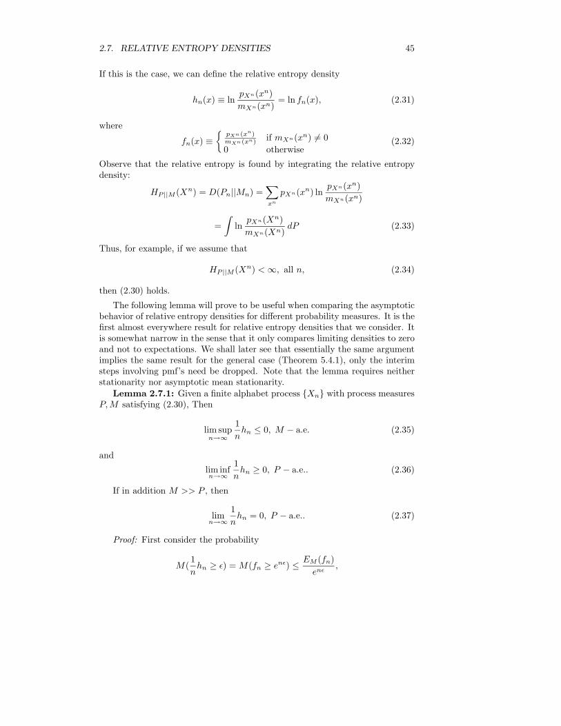
2.7. RELATIVE ENTROPY DENSITIES 45
If this is the case, we can define the relative entropy density
hn(x) ≡ lnpXn(xn)mXn(xn)
= ln fn(x), (2.31)
where
fn(x) ≡
pXn (xn)mXn (xn) if mXn(xn) 6= 00 otherwise
(2.32)
Observe that the relative entropy is found by integrating the relative entropydensity:
HP ||M (Xn) = D(Pn||Mn) =∑xn
pXn(xn) lnpXn(xn)mXn(xn)
=∫
lnpXn(Xn)mXn(Xn)
dP (2.33)
Thus, for example, if we assume that
HP ||M (Xn) < ∞, all n, (2.34)
then (2.30) holds.
The following lemma will prove to be useful when comparing the asymptoticbehavior of relative entropy densities for different probability measures. It is thefirst almost everywhere result for relative entropy densities that we consider. Itis somewhat narrow in the sense that it only compares limiting densities to zeroand not to expectations. We shall later see that essentially the same argumentimplies the same result for the general case (Theorem 5.4.1), only the interimsteps involving pmf’s need be dropped. Note that the lemma requires neitherstationarity nor asymptotic mean stationarity.
Lemma 2.7.1: Given a finite alphabet process Xn with process measuresP,M satisfying (2.30), Then
lim supn→∞
1n
hn ≤ 0, M − a.e. (2.35)
and
lim infn→∞
1n
hn ≥ 0, P − a.e.. (2.36)
If in addition M >> P , then
limn→∞
1n
hn = 0, P − a.e.. (2.37)
Proof: First consider the probability
M(1n
hn ≥ ε) = M(fn ≥ enε) ≤ EM (fn)enε
,
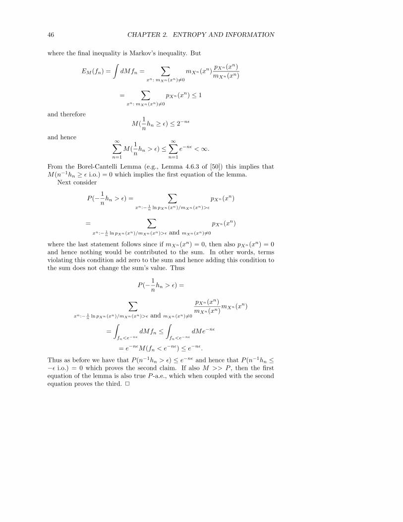
46 CHAPTER 2. ENTROPY AND INFORMATION
where the final inequality is Markov’s inequality. But
EM (fn) =∫
dMfn =∑
xn: mXn (xn) 6=0
mXn(xn)pXn(xn)mXn(xn)
=∑
xn: mXn (xn) 6=0
pXn(xn) ≤ 1
and thereforeM(
1n
hn ≥ ε) ≤ 2−nε
and hence ∞∑n=1
M(1n
hn > ε) ≤∞∑
n=1
e−nε < ∞.
From the Borel-Cantelli Lemma (e.g., Lemma 4.6.3 of [50]) this implies thatM(n−1hn ≥ ε i.o.) = 0 which implies the first equation of the lemma.
Next consider
P (− 1n
hn > ε) =∑
xn:− 1n ln pXn (xn)/mXn (xn)>ε
pXn(xn)
=∑
xn:− 1n ln pXn (xn)/mXn (xn)>ε and mXn (xn) 6=0
pXn(xn)
where the last statement follows since if mXn(xn) = 0, then also pXn(xn) = 0and hence nothing would be contributed to the sum. In other words, termsviolating this condition add zero to the sum and hence adding this condition tothe sum does not change the sum’s value. Thus
P (− 1n
hn > ε) =
∑xn:− 1
n ln pXn (xn)/mXn (xn)>ε and mXn (xn) 6=0
pXn(xn)mXn(xn)
mXn(xn)
=∫
fn<e−nε
dMfn ≤∫
fn<e−nε
dMe−nε
= e−nεM(fn < e−nε) ≤ e−nε.
Thus as before we have that P (n−1hn > ε) ≤ e−nε and hence that P (n−1hn ≤−ε i.o.) = 0 which proves the second claim. If also M >> P , then the firstequation of the lemma is also true P -a.e., which when coupled with the secondequation proves the third. 2
Chapter 3
The Entropy ErgodicTheorem
3.1 Introduction
The goal of this chapter is to prove an ergodic theorem for sample entropy offinite alphabet random processes. The result is sometimes called the ergodictheorem of information theory or the asymptotic equipartion theorem, but it isbest known as the Shannon-McMillan-Breiman theorem. It provides a commonfoundation to many of the results of both ergodic theory and information the-ory. Shannon [129] first developed the result for convergence in probability forstationary ergodic Markov sources. McMillan [103] proved L1 convergence forstationary ergodic sources and Breiman [19] [20] proved almost everywhere con-vergence for stationary and ergodic sources. Billingsley [15] extended the resultto stationary nonergodic sources. Jacobs [67] [66] extended it to processes dom-inated by a stationary measure and hence to two-sided AMS processes. Grayand Kieffer [54] extended it to processes asymptotically dominated by a sta-tionary measure and hence to all AMS processes. The generalizations to AMSprocesses build on the Billingsley theorem for the stationary mean. Follow-ing generalizations of the definitions of entropy and information, correspondinggeneralizations of the entropy ergodic theorem will be considered in Chapter 8.
Breiman’s and Billingsley’s approach requires the martingale convergencetheorem and embeds the possibly one-sided stationary process into a two-sidedprocess. Ornstein and Weiss [117] recently developed a proof for the stationaryand ergodic case that does not require any martingale theory and considersonly positive time and hence does not require any embedding into two-sidedprocesses. The technique was described for both the ordinary ergodic theoremand the entropy ergodic theorem by Shields [132]. In addition, it uses a formof coding argument that is both more direct and more information theoretic inflavor than the traditional martingale proofs. We here follow the Ornstein andWeiss approach for the stationary ergodic result. We also use some modifications
47
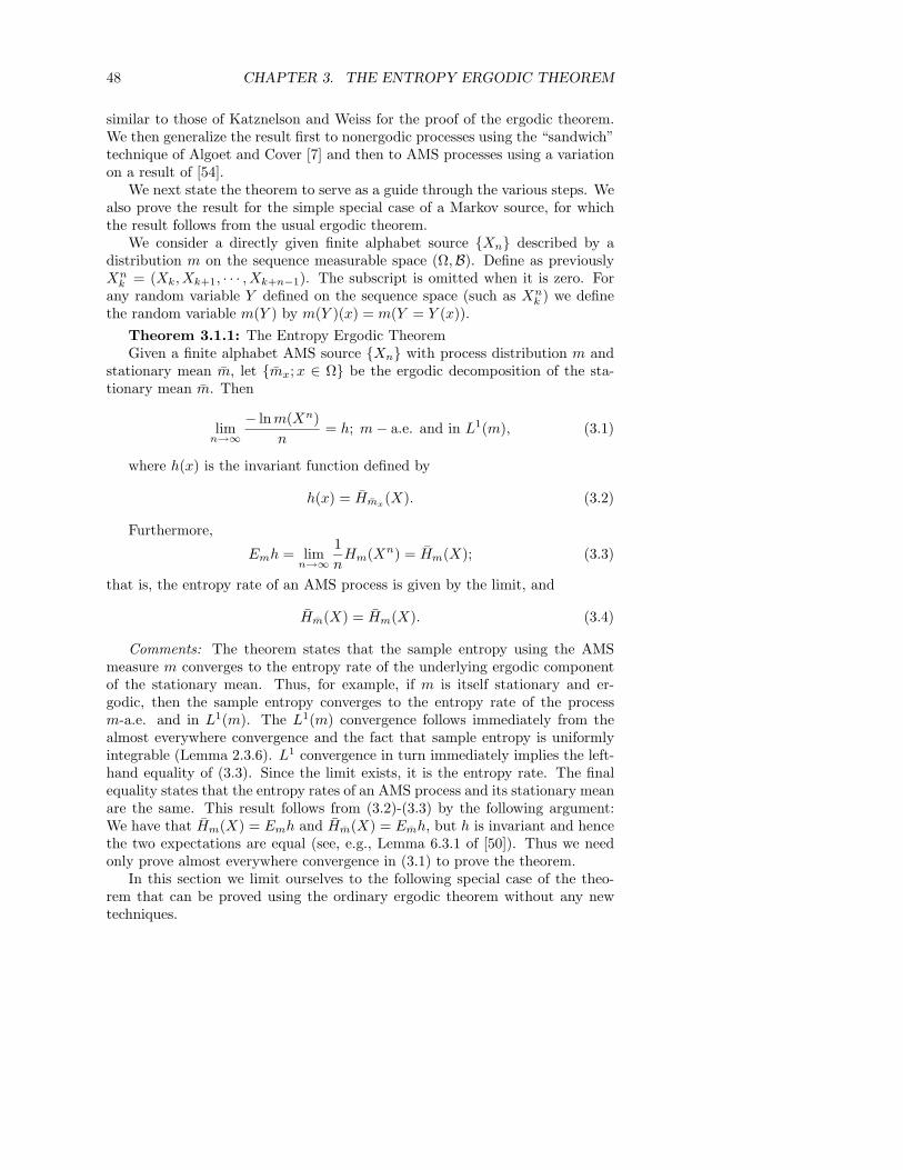
48 CHAPTER 3. THE ENTROPY ERGODIC THEOREM
similar to those of Katznelson and Weiss for the proof of the ergodic theorem.We then generalize the result first to nonergodic processes using the “sandwich”technique of Algoet and Cover [7] and then to AMS processes using a variationon a result of [54].
We next state the theorem to serve as a guide through the various steps. Wealso prove the result for the simple special case of a Markov source, for whichthe result follows from the usual ergodic theorem.
We consider a directly given finite alphabet source Xn described by adistribution m on the sequence measurable space (Ω,B). Define as previouslyXn
k = (Xk, Xk+1, · · · , Xk+n−1). The subscript is omitted when it is zero. Forany random variable Y defined on the sequence space (such as Xn
k ) we definethe random variable m(Y ) by m(Y )(x) = m(Y = Y (x)).
Theorem 3.1.1: The Entropy Ergodic TheoremGiven a finite alphabet AMS source Xn with process distribution m and
stationary mean m, let mx;x ∈ Ω be the ergodic decomposition of the sta-tionary mean m. Then
limn→∞
− ln m(Xn)n
= h; m − a.e. and in L1(m), (3.1)
where h(x) is the invariant function defined by
h(x) = Hmx(X). (3.2)
Furthermore,
Emh = limn→∞
1n
Hm(Xn) = Hm(X); (3.3)
that is, the entropy rate of an AMS process is given by the limit, and
Hm(X) = Hm(X). (3.4)
Comments: The theorem states that the sample entropy using the AMSmeasure m converges to the entropy rate of the underlying ergodic componentof the stationary mean. Thus, for example, if m is itself stationary and er-godic, then the sample entropy converges to the entropy rate of the processm-a.e. and in L1(m). The L1(m) convergence follows immediately from thealmost everywhere convergence and the fact that sample entropy is uniformlyintegrable (Lemma 2.3.6). L1 convergence in turn immediately implies the left-hand equality of (3.3). Since the limit exists, it is the entropy rate. The finalequality states that the entropy rates of an AMS process and its stationary meanare the same. This result follows from (3.2)-(3.3) by the following argument:We have that Hm(X) = Emh and Hm(X) = Emh, but h is invariant and hencethe two expectations are equal (see, e.g., Lemma 6.3.1 of [50]). Thus we needonly prove almost everywhere convergence in (3.1) to prove the theorem.
In this section we limit ourselves to the following special case of the theo-rem that can be proved using the ordinary ergodic theorem without any newtechniques.
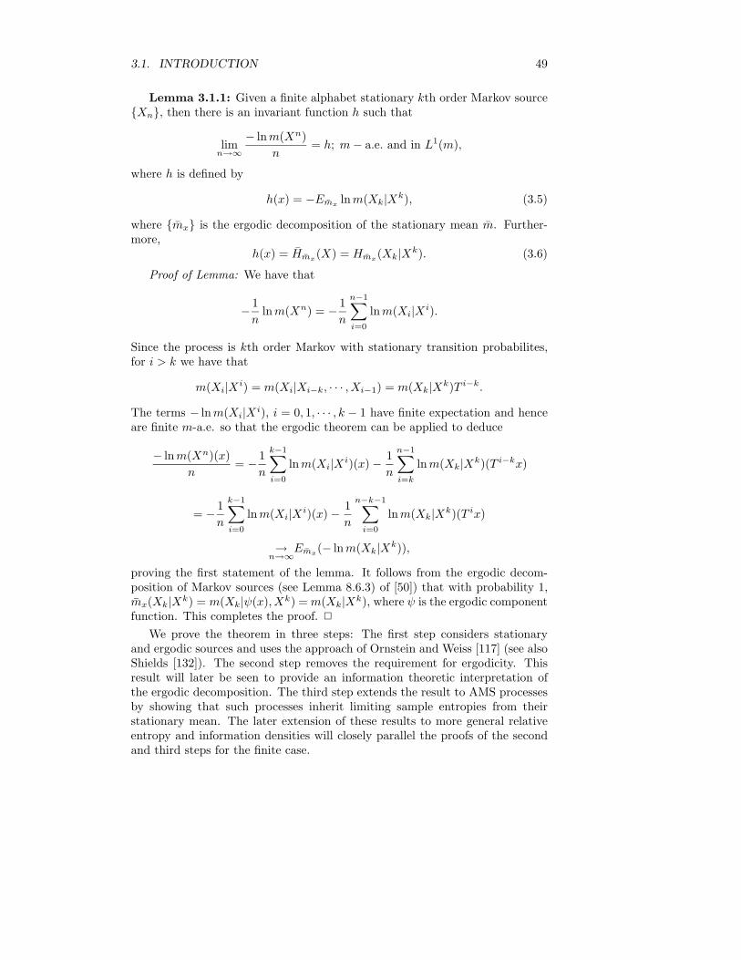
3.1. INTRODUCTION 49
Lemma 3.1.1: Given a finite alphabet stationary kth order Markov sourceXn, then there is an invariant function h such that
limn→∞
− lnm(Xn)n
= h; m − a.e. and in L1(m),
where h is defined by
h(x) = −Emxlnm(Xk|Xk), (3.5)
where mx is the ergodic decomposition of the stationary mean m. Further-more,
h(x) = Hmx(X) = Hmx
(Xk|Xk). (3.6)
Proof of Lemma: We have that
− 1n
lnm(Xn) = − 1n
n−1∑i=0
lnm(Xi|Xi).
Since the process is kth order Markov with stationary transition probabilites,for i > k we have that
m(Xi|Xi) = m(Xi|Xi−k, · · · , Xi−1) = m(Xk|Xk)T i−k.
The terms − lnm(Xi|Xi), i = 0, 1, · · · , k − 1 have finite expectation and henceare finite m-a.e. so that the ergodic theorem can be applied to deduce
− lnm(Xn)(x)n
= − 1n
k−1∑i=0
lnm(Xi|Xi)(x) − 1n
n−1∑i=k
lnm(Xk|Xk)(T i−kx)
= − 1n
k−1∑i=0
lnm(Xi|Xi)(x) − 1n
n−k−1∑i=0
lnm(Xk|Xk)(T ix)
→n→∞
Emx(− ln m(Xk|Xk)),
proving the first statement of the lemma. It follows from the ergodic decom-position of Markov sources (see Lemma 8.6.3) of [50]) that with probability 1,mx(Xk|Xk) = m(Xk|ψ(x), Xk) = m(Xk|Xk), where ψ is the ergodic componentfunction. This completes the proof. 2
We prove the theorem in three steps: The first step considers stationaryand ergodic sources and uses the approach of Ornstein and Weiss [117] (see alsoShields [132]). The second step removes the requirement for ergodicity. Thisresult will later be seen to provide an information theoretic interpretation ofthe ergodic decomposition. The third step extends the result to AMS processesby showing that such processes inherit limiting sample entropies from theirstationary mean. The later extension of these results to more general relativeentropy and information densities will closely parallel the proofs of the secondand third steps for the finite case.
50 CHAPTER 3. THE ENTROPY ERGODIC THEOREM
3.2 Stationary Ergodic Sources
This section is devoted to proving the entropy ergodic theorem for the specialcase of stationary ergodic sources. The result was originally proved by Breiman[19]. The original proof first used the martingale convergence theorem to inferthe convergence of conditional probabilities of the form m(X0|X−1, X−2, · · · , X−k)to m(X0|X−1, X−2, · · ·). This result was combined with an an extended form ofthe ergodic theorem stating that if gk → g as k → ∞ and if gk is L1-dominated(supk |gk| is in L1), then 1/n
∑n−1k=0 gkT k has the same limit as 1/n
∑n−1k=0 gT k.
Combining these facts yields that that
1n
lnm(Xn) =1n
n−1∑k=0
lnm(Xk|Xk)
=1n
n−1∑k=0
lnm(X0|Xk−k)T k
has the same limit as
1n
n−1∑k=0
lnm(X0|X−1, X−2, · · ·)T k
which, from the usual ergodic theorem, is the expectation
E(lnm(X0|X−) ≡ E(lnm(X0|X−1, X−2, · · ·)).
As suggested at the end of the preceeding chapter, this should be minus theconditional entropy H(X0|X−1, X−2, · · ·) which in turn should be the entropyrate HX . This approach has three shortcomings: it requires a result from mar-tingale theory which has not been proved here or in the companion volume [50],it requires an extended ergodic theorem which has similarly not been provedhere, and it requires a more advanced definition of entropy which has not yetbeen introduced. Another approach is the sandwich proof of Algoet and Cover[7]. They show without using martingale theory or the extended ergodic theo-rem that 1/n
∑n−1i=0 lnm(X0|Xi
−i)Ti is asymptotically sandwiched between the
entropy rate of a kth order Markov approximation:
1n
n−1∑i=k
lnm(X0|Xk−k)T i → Em[lnm(X0|Xk
−k)] = −H(X0|Xk−k)
and1n
n−1∑i=k
lnm(X0|X−1, X−2, · · ·)T i → Em[lnm(X0|X1, · · ·)]
= −H(X0|X−1, X−2, · · ·).By showing that these two limits are arbitrarily close as k → ∞, the result isproved. The drawback of this approach for present purposes is that again the
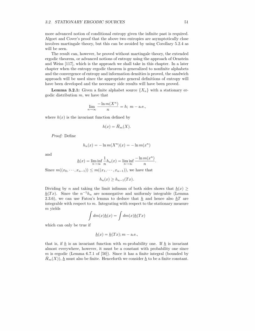
3.2. STATIONARY ERGODIC SOURCES 51
more advanced notion of conditional entropy given the infinite past is required.Algoet and Cover’s proof that the above two entropies are asymptotically closeinvolves martingale theory, but this can be avoided by using Corollary 5.2.4 aswill be seen.
The result can, however, be proved without martingale theory, the extendedergodic theorem, or advanced notions of entropy using the approach of Ornsteinand Weiss [117], which is the approach we shall take in this chapter. In a laterchapter when the entropy ergodic theorem is generalized to nonfinite alphabetsand the convergence of entropy and information densities is proved, the sandwichapproach will be used since the appropriate general definitions of entropy willhave been developed and the necessary side results will have been proved.
Lemma 3.2.1: Given a finite alphabet source Xn with a stationary er-godic distribution m, we have that
limn→∞
− lnm(Xn)n
= h; m − a.e.,
where h(x) is the invariant function defined by
h(x) = Hm(X).
Proof: Define
hn(x) = − lnm(Xn)(x) = − ln m(xn)
and
h(x) = lim infn→∞
1n
hn(x) = lim infn→∞
− lnm(xn)n
.
Since m((x0, · · · , xn−1)) ≤ m((x1, · · · , xn−1)), we have that
hn(x) ≥ hn−1(Tx).
Dividing by n and taking the limit infimum of both sides shows that h(x) ≥h(Tx). Since the n−1hn are nonnegative and uniformly integrable (Lemma2.3.6), we can use Fatou’s lemma to deduce that h and hence also hT areintegrable with respect to m. Integrating with respect to the stationary measurem yields ∫
dm(x)h(x) =∫
dm(x)h(Tx)
which can only be true if
h(x) = h(Tx);m − a.e.,
that is, if h is an invariant function with m-probability one. If h is invariantalmost everywhere, however, it must be a constant with probability one sincem is ergodic (Lemma 6.7.1 of [50]). Since it has a finite integral (bounded byHm(X)), h must also be finite. Henceforth we consider h to be a finite constant.
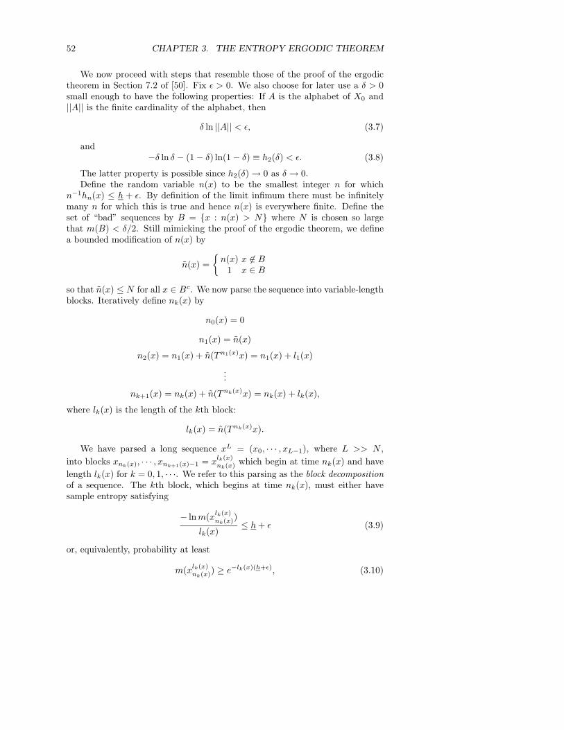
52 CHAPTER 3. THE ENTROPY ERGODIC THEOREM
We now proceed with steps that resemble those of the proof of the ergodictheorem in Section 7.2 of [50]. Fix ε > 0. We also choose for later use a δ > 0small enough to have the following properties: If A is the alphabet of X0 and||A|| is the finite cardinality of the alphabet, then
δ ln ||A|| < ε, (3.7)
and−δ ln δ − (1 − δ) ln(1 − δ) ≡ h2(δ) < ε. (3.8)
The latter property is possible since h2(δ) → 0 as δ → 0.Define the random variable n(x) to be the smallest integer n for which
n−1hn(x) ≤ h + ε. By definition of the limit infimum there must be infinitelymany n for which this is true and hence n(x) is everywhere finite. Define theset of “bad” sequences by B = x : n(x) > N where N is chosen so largethat m(B) < δ/2. Still mimicking the proof of the ergodic theorem, we definea bounded modification of n(x) by
n(x) =
n(x)1
x 6∈ Bx ∈ B
so that n(x) ≤ N for all x ∈ Bc. We now parse the sequence into variable-lengthblocks. Iteratively define nk(x) by
n0(x) = 0
n1(x) = n(x)
n2(x) = n1(x) + n(Tn1(x)x) = n1(x) + l1(x)
...
nk+1(x) = nk(x) + n(Tnk(x)x) = nk(x) + lk(x),
where lk(x) is the length of the kth block:
lk(x) = n(Tnk(x)x).
We have parsed a long sequence xL = (x0, · · · , xL−1), where L >> N ,into blocks xnk(x), · · · , xnk+1(x)−1 = x
lk(x)nk(x) which begin at time nk(x) and have
length lk(x) for k = 0, 1, · · ·. We refer to this parsing as the block decompositionof a sequence. The kth block, which begins at time nk(x), must either havesample entropy satisfying
− lnm(xlk(x)nk(x))
lk(x)≤ h + ε (3.9)
or, equivalently, probability at least
m(xlk(x)nk(x)) ≥ e−lk(x)(h+ε), (3.10)
3.2. STATIONARY ERGODIC SOURCES 53
or it must consist of only a single symbol. Blocks having length 1 (lk = 1)could have the correct sample entropy, that is,
− ln m(x1nk(x))
1≤ h + ε,
or they could be bad in the sense that they are the first symbol of a sequencewith n > N ; that is,
n(Tnk(x)x) > N,
or, equivalently,Tnk(x)x ∈ B.
Except for these bad symbols, each of the blocks by construction will have aprobability which satisfies the above bound.
Define for nonnegative integers n and positive integers l the sets
S(n, l) = x : m(X ln(x)) ≥ e−l(h+ε),
that is, the collection of infinite sequences for which (3.2.2) and (3.2.3) hold fora block starting at n and having length l. Observe that for such blocks therecannot be more than el(h+ε) distinct l-tuples for which the bound holds (lestthe probabilities sum to something greater than 1). In symbols this is
||S(n, l)|| ≤ el(h+ε). (3.11)
The ergodic theorem will imply that there cannot be too many single symbolblocks with n(Tnk(x)x) > N because the event has small probability. Thesefacts will be essential to the proof.
Even though we write n(x) as a function of the entire infinite sequence, wecan determine its value by observing only the prefix xN of x since either thereis an n ≤ N for which n−1 lnm(xn) ≤ h + ε or there is not. Hence there is afunction n(xN ) such that n(x) = n(xN ). Define the finite length sequence eventC = xN : n(xN ) = 1 and − ln m(x1) > h + ε, that is, C is the collection of allN -tuples xN that are prefixes of bad infinite sequences, sequences x for whichn(x) > N . Thus in particular,
x ∈ B if and only if xN ∈ C. (3.12)
Now recall that we parse sequences of length L >> N and define the set GL
of “good” L-tuples by
GL = xL :1
L − N
L−N−1∑i=0
1C(xNi ) ≤ δ,
that is, GL is the collection of all L-tuples which have fewer than δ(L−N) ≤ δLtime slots i for which xN
i is a prefix of a bad infinite sequence. From (3.12) and
54 CHAPTER 3. THE ENTROPY ERGODIC THEOREM
the ergodic theorem for stationary ergodic sources we know that m-a.e. we getan x for which
limn→∞
1n
n−1∑i=0
1C(xNi ) = lim
n→∞
1n
n−1∑i=0
1B(T ix) = m(B) ≤ δ
2. (3.13)
From the definition of a limit, this means that with probability 1 we get an xfor which there is an L0 = L0(x) such that
1L − N
L−N−1∑i=0
1C(xNi ) ≤ δ; for all L > L0. (3.14)
This follows simply because if the limit is less than δ/2, there must be an L0 solarge that for larger L the time average is at least no greater than 2δ/2 = δ. Wecan restate (3.14) as follows: with probability 1 we get an x for which xL ∈ GL
for all but a finite number of L. Stating this in negative fashion, we have one ofthe key properties required by the proof: If xL ∈ GL for all but a finite numberof L, then xL cannot be in the complement Gc
L infinitely often, that is,
m(x : xL ∈ GcL i.o.) = 0. (3.15)
We now change tack to develop another key result for the proof. For eachL we bounded above the cardinality ||GL|| of the set of good L-tuples. Byconstruction there are no more than δL bad symbols in an L-tuple in GL andthese can occur in any of at most
∑k≤δL
(Lk
)≤ eh2(δ)L (3.16)
places, where we have used Lemma 2.3.5. Eq. (3.16) provides an upperbound on the number of ways that a sequence in GL can be parsed by the givenrules. The bad symbols and the final N symbols in the L-tuple can take onany of the ||A|| different values in the alphabet. Eq. (3.11) bounds the numberof finite length sequences that can occur in each of the remaining blocks andhence for any given block decomposition, the number of ways that the remainingblocks blocks can be filled is bounded above by
∏k:T nk(x)x6∈B
elk(x)(h+ε) = e∑
klk(x)(h+ε) = eL(h+ε), (3.17)
regardless of the details of the parsing. Combining these bounds we have that
||GL|| ≤ eh2(δ)L × ||A||δL × ||A||N × eL(h+ε) = eh2(δ)L+(δL+N) ln ||A||+L(h+ε)
or||GL|| ≤ eL(h+ε+h2(δ)+(δ+ N
L ) ln ||A||).
3.2. STATIONARY ERGODIC SOURCES 55
Since δ satisfies (3.7)–(3.8), we can choose L1 large enough so that N ln ||A||/L1 ≤ε and thereby obtain
||GL|| ≤ eL(h+4ε); L ≥ L1. (3.18)
This bound provides the second key result in the proof of the lemma. We nowcombine (3.18) and (3.15) to complete the proof.
Let BL denote a collection of L-tuples that are bad in the sense of havingtoo large a sample entropy or, equivalently, too small a probability; that is ifxL ∈ BL, then
m(xL) ≤ e−L(h+5ε)
or, equivalently, for any x with prefix xL
hL(x) ≥ h + 5ε.
The upper bound on ||GL|| provides a bound on the probability of BL
⋂GL:
m(BL
⋂GL) =
∑xL∈BL
⋂GL
m(xL) ≤∑
xL∈GL
e−L(h+5ε)
≤ ||GL||e−L(h+5ε) ≤ e−εL.
Recall now that the above bound is true for a fixed ε > 0 and for all L ≥ L1.Thus
∞∑L=1
m(BL
⋂GL) =
L1−1∑L=1
m(BL
⋂GL) +
∞∑L=L1
m(BL
⋂GL)
≤ L1 +∞∑
L=L1
e−εL < ∞
and hence from the Borel-Cantelli lemma (Lemma 4.6.3 of [50]) m(x : xL ∈BL
⋂GL i.o.) = 0. We also have from (3.2.8), however, that m(x : xL ∈
GcL i.o. ) = 0 and hence xL ∈ GL for all but a finite number of L. Thus
xL ∈ BL i.o. if and only if xL ∈ BL
⋂GL i.o. As this latter event has zero
probability, we have shown that m(x : xL ∈ BL i.o.) = 0 and hence
lim supL→∞
hL(x) ≤ h + 5ε.
Since ε is arbitrary we have proved that the limit supremum of the sampleentropy −n−1 lnm(Xn) is less than or equal to the limit infimum and thereforethat the limit exists and hence with m-probability 1
limn→∞
− lnm(Xn)n
= h. (3.19)
Since the terms on the left in (3.19) are uniformly integrable from Lemma2.3.6, we can integrate to the limit and apply Lemma 2.4.1 to find that
h = limn→∞
∫dm(x)
− ln m(Xn(x))n
= Hm(X),
56 CHAPTER 3. THE ENTROPY ERGODIC THEOREM
which completes the proof of the lemma and hence also proves Theorem 3.1.1for the special case of stationary ergodic measures. 2
3.3 Stationary Nonergodic Sources
Next suppose that a source is stationary with ergodic decomposition mλ; λ ∈Λ and ergodic component function ψ as in Theorem 1.8.3. The source willproduce with probability one under m an ergodic component mλ and Lemma3.2.2 will hold for this ergodic component. In other words, we should have that
limn→∞
− 1n
lnmψ(Xn) = Hmψ(X); m − a.e., (3.20)
that is,m(x : − lim
n→∞lnmψ(x)(xn) = Hmψ(x)(X)) = 1.
This argument is made rigorous in the following lemma.Lemma 3.3.1: Suppose that Xn is a stationary not necessarily ergodic
source with ergodic component function ψ. Then
m(x : − limn→∞
lnmψ(x)(xn) = Hmψ(x)(X)) = 1; m − a.e.. (3.21)
Proof: Let
G = x : − limn→∞
lnmψ(x)(xn) = Hmψ(x)(X)
and let Gλ denote the section of G at λ, that is,
Gλ = x : − limn→∞
lnmλ(xn) = Hmλ(X).
From the ergodic decomposition (e.g., Theorem 1.8.3 or [50], Theorem 8.5.1)and (1.26)
m(G) =∫
dPψ(λ)mλ(G),
wheremλ(G) = m(G|ψ = λ) = m(G
⋂x : ψ(x) = λ|ψ = λ)
= m(Gλ|ψ = λ) = mλ(Gλ)
which is 1 for all λ from the stationary ergodic result. Thus
m(G) =∫
dPψ(λ)mλ(Gλ) = 1.
It is straightforward to verify that all of the sets considered are in fact measur-able. 2
Unfortunately it is not the sample entropy using the distribution of theergodic component that is of interest, rather it is the original sample entropy
3.3. STATIONARY NONERGODIC SOURCES 57
for which we wish to prove convergence. The following lemma shows that thetwo sample entropies converge to the same limit and hence Lemma 3.3.1 will alsoprovide the limit of the sample entropy with respect to the stationary measure.
Lemma 3.3.2: Given a stationary source Xn, let mλ; λ ∈ Λ denotethe ergodic decomposition and ψ the ergodic component function of Theorem1.8.3. Then
limn→∞
1n
lnmψ(Xn)m(Xn)
= 0; m − a.e.
Proof: First observe that if m(an) is 0, then from the ergodic decompositionwith probability 1 mψ(an) will also be 0. One part is easy. For any ε > 0 wehave from the Markov inequality that
m(1n
lnm(Xn)mψ(Xn)
> ε) = m(m(Xn)mψ(Xn)
> enε)
≤ Em(m(Xn)mψ(Xn)
)e−nε.
The expectation, however, can be evaluated as follows: Let A(λ)n = an :
mλ(an) > 0. Then
Em
(m(Xn)mψ(Xn)
)=
∫dPψ(λ)
∑an∈An
m(an)mλ(an)
mλ(an)
=∫
dPψ(λ)m(A(λ)n ) ≤ 1,
where Pψ is the distribution of ψ. Thus
m(1n
lnm(Xn)mψ(Xn)
> ε) ≤ e−nε.
and hence ∞∑n=1
m(1n
lnm(Xn)mψ(Xn)
> ε) < ∞
and hence from the Borel-Cantelli lemma
m(1n
lnm(Xn)mψ(Xn)
> ε i.o.) = 0
and hence with m probability 1
lim supn→∞
1n
lnm(Xn)mψ(Xn)
≤ ε.
Since ε is arbitrary,
lim supn→∞
1n
lnm(Xn)mψ(Xn)
≤ 0; m − a.e.. (3.22)
58 CHAPTER 3. THE ENTROPY ERGODIC THEOREM
For later use we restate this as
lim infn→∞
1n
lnmψ(Xn)m(Xn)
≥ 0; m − a.e.. (3.23)
We now turn to the converse inequality. For any positive integer k, we canconstruct a stationary k-step Markov approximation to m as in Section 2.6, thatis, construct a process m(k) with the conditional probabilities
m(k)(Xn ∈ F |Xn) = m(k)(Xn ∈ F |Xkn−k)
= m(Xn ∈ F |Xkn−k)
and the same kth order distributions m(k)(Xk ∈ F ) = m(Xk ∈ F ). Considerthe probability
m(1n
lnm(k)(Xn)m(Xn)
≥ ε) = m(m(k)(Xn)m(Xn)
≥ enε)
≤ Em(m(k)(Xn)m(Xn)
)e−nε.
The expectation is evaluated as
∑xn
m(k)(xn)m(xn)
m(xn) = 1
and hence we again have using Borel-Cantelli that
lim supn→∞
1n
lnm(k)(Xn)m(Xn)
≤ 0.
We can apply the usual ergodic theorem to conclude that with probability 1under m
lim supn→∞
1n
ln1
m(Xn)≤ lim
n→∞
1n
ln1
m(k)(Xn)= Emψ
[− ln m(Xk|Xk)].
Combining this result with (3.20) we have using Lemma 2.4.3 that
lim supn→∞
1n
lnmψ(Xn)m(Xn)
≤ −Hmψ(X) − Emψ
[lnm(Xk|Xk)].
= Hmψ||m(k)(X). (3.24)
This bound holds for any integer k and hence it must also be true that m-a.e.the following holds:
lim supn→∞
1n
lnmψ(Xn)m(Xn)
≤ infk
Hmψ||m(k)(X) ≡ ζ. (3.25)
3.4. AMS SOURCES 59
In order to evaluate ζ we apply the ergodic decomposition of relative entropyrate (Corollary 2.4.2) and the ordinary ergodic decomposition to write∫
dPψζ =∫
dPψ infk
Hmψ||m(k)(X)
≤ infk
∫dPψHmψ||m(k)(X) = inf
kHm||m(k)(X).
From Theorem 2.6.2, the right hand term is 0. If the integral of a nonnegativefunction is 0, the integrand must itself be 0 with probability one. Thus (3.25)becomes
lim supn→∞
1n
lnmψ(Xn)m(Xn)
≤ 0,
which with (3.23) completes the proof of the lemma. 2
We shall later see that the quantity
in(Xn;ψ) =1n
lnmψ(Xn)m(Xn)
is the sample mutual information (in a generalized sense so that it applies to theusually non-discrete ψ) and hence the lemma states that the normalized samplemutual information between the process outputs and the ergodic componentfunction goes to 0 as the number of samples goes to infinity.
The two previous lemmas immediately yield the following result.Corollary 3.3.1: The conclusions of Theorem 3.1.1 hold for sources that
are stationary.
3.4 AMS Sources
The principal idea required to extend the entropy theorem from stationarysources to AMS sources is contained in Lemma 3.4.2. It shows that an AMSsource inherits sample entropy properties from an asymptotically dominatingstationary source (just as it inherits ordinary ergodic properties from such asource). The result is originally due to Gray and Kieffer [54], but the proofhere is somewhat different. The tough part here is handling the fact that thesample average being considered depends on a specific measure. From Theorem1.7.1, the stationary mean of an AMS source dominates the original source ontail events, that is, events in F∞. We begin by showing that certain importantevents can be recast as tail events, that is, they can be determined by lookingat only samples in the arbitrarily distant future. The following result is of thisvariety: It implies that sample entropy is unaffected by the starting time.
Lemma 3.4.1: Let Xn be a finite alphabet source with distribution m.Recall that Xn
k = (Xk, Xk+1, · · · , Xk+n−1) and define the information density
i(Xk;Xn−kk ) = ln
m(Xn)m(Xk)m(Xn−k
k ).
60 CHAPTER 3. THE ENTROPY ERGODIC THEOREM
Thenlim
n→∞
1n
i(Xk;Xn−kk ) = 0; m − a.e..
Comment: The lemma states that with probability 1 the per-sample mutualinformation density between the first k samples and future samples goes to zeroin the limit. Equivalently, limits of n−1 lnm(Xn) will be the same as limits ofn−1 lnm(Xn−k
k ) for any finite k. Note that the result does not require even thatthe source be AMS. The lemma is a direct consequence of Lemma 2.7.1.
Proof: Define the distribution p = mXk ×mXk,Xk+1,···, that is, a distributionfor which all samples after the first k are independent of the first k samples.Thus, in particular, p(Xn) = m(Xk)m(Xn
k ). We will show that p >> m, inwhich case the lemma will follow from Lemma 2.7.1. Suppose that p(F ) = 0. Ifwe denote X+
k = Xk, Xk+1, · · ·, then
0 = p(F ) =∑xk
m(xk)mX+k
(Fxk),
where Fxk is the section x+k : (xk, x+
k ) = x ∈ F. For the above relation tohold, we must have mX+
k(Fxk) = 0 for all xk with m(xk) 6= 0. We also have,
however, thatm(F ) =
∑ak
m(Xk = ak, X+k ∈ Fak)
=∑ak
m(Xk = ak|X+k ∈ Fak)m(X+
k ∈ Fak).
But this sum must be 0 since the rightmost terms are 0 for all ak for whichm(Xk = ak) is not 0. (Observe that we must have m(Xk = ak|X+
k ∈ Fak) =0 if m(X+
k ∈ Fak) 6= 0 since otherwise m(Xk = ak) ≥ m(Xk = ak, X+k ∈ Fak)
> 0, yielding a contradiction.) Thus p >> m and the lemma is proved. 2
For later use we note that we have shown that a joint distribution is dom-inated by a product of its marginals if one of the marginal distributions isdiscrete.
Lemma 3.4.2: Suppose that Xn is an AMS source with distribution mand suppose that m is a stationary source that asymptotically dominates m(e.g., m is the stationary mean). If there is an invariant function h such that
limn→∞
− 1n
ln m(Xn) = h; m − a.e.,
then also,
limn→∞
− 1n
lnm(Xn) = h; m − a.e.
Proof: For any k we can write using the chain rule for densities
− 1n
lnm(Xn) +1n
lnm(Xn−kk ) = − 1
nlnm(Xk|Xn−k
k )
3.4. AMS SOURCES 61
= − 1n
i(Xk;Xn−kk ) − 1
nlnm(Xk).
From the previous lemma and from the fact that Hm(Xk) = −Em lnm(Xk) isfinite, the right hand terms converge to 0 as n → ∞ and hence for any k
limn→∞
− 1n
lnm(Xk|Xn−kk )
= limn→∞
(− 1n
lnm(Xn) +1n
lnm(Xn−kk )) = 0; m − a.e.. (3.26)
This implies that there is a subsequence k(n) → ∞ such that
− 1n
lnm(Xk(n)|Xn−k(n)k(n) )
= − 1n
lnm(Xn) − 1n
lnm(Xn−kk(n) (n)) → 0; m − a.e.. (3.27)
To see this, observe that (3.26) ensures that for each k there is an N(k) largeenough so that N(k) > N(k − 1) and
m(| − 1N(k)
lnm(Xk|XN(k)−kk )| > 2−k) ≤ 2−k. (3.28)
Applying the Borel-Cantelli lemma implies that for any ε,
m(| − 1/N(k) ln m(Xk|XN(k)−kk )| > ε i.o.) = 0.
Now let k(n) = k for N(k) ≤ n < N(k + 1). Then
m(| − 1/n ln m(Xk(n)|Xn−k(n)k(n) )| > ε i.o.) = 0
and therefore
limn→∞
(− 1
nlnm(Xn) +
1n
lnm(Xn−k(n)k(n) )
)= 0; m − a.e.
as claimed in (3.27).In a similar manner we can also choose the sequence so that
limn→∞
(− 1
nln m(Xn) +
1n
ln m(Xn−k(n)k(n) )
)= 0; m − a.e.,
that is, we can choose N(k) so that (3.4.3) simultaneously holds for both m andm. Invoking the entropy ergodic theorem for the stationary m (Corollary 3.3.1)we have therefore that
limn→∞
− 1n
ln m(Xn−k(n)k(n) ) = h; m − a.e.. (3.29)
62 CHAPTER 3. THE ENTROPY ERGODIC THEOREM
From Markov’s inequality (Lemma 4.4.3 of [50])
m(− 1n
lnm(Xnk ) ≤ − 1
nln m(Xn
k ) − ε) = m(m(Xn
k )m(Xn
k )≥ enε)
≤ e−nεEmm(Xn−k
k )m(Xn−k
k )= e−nε
∑xn−k
k:m(xn−k
k) 6=0
m(xn−kk )
m(xn−kk )
m(xn−kk ) ≤ e−nε.
Hence taking k = k(n) and again invoking the Borel-Cantelli lemma we havethat
m(− 1n
lnm(Xn−k(n)k(n) ) ≤ − 1
nln m(Xn−k(n)
k(n) ) − ε i.o.) = 0
or, equivalently, that
lim infn→∞
− 1n
lnm(Xn−k(n)
k(n) )
m(Xn−k(n)k(n) )
≥ 0; m − a.e.. (3.30)
Therefore from (3.29)
lim infn→∞
− 1n
lnm(Xn−k(n)k(n) ) ≥ h; m − a.e.. (3.31)
The above event is in the tail σ-field F∞ =⋂
n σ(Xn, Xn+1, · · ·) since it can bedetermined from Xk(n), · · · for arbitrarily large n and since h is invariant. Sincem dominates m on the tail σ-field (Theorem 1.7.2), we have also
lim infn→∞
− 1n
lnm(Xn−k(n)k(n) ) ≥ h; m − a.e.
and hence by (3.4.2)
lim infn→∞
− 1n
lnm(Xn) ≥ h; m − a.e.
which proves half of the lemma.Since
m( limn→∞
− 1n
ln m(Xn) 6= h) = 0
and since m asymptotically dominates m (Theorem 1.7.1), given ε > 0 there isa k such that
m( limn→∞
− 1n
ln m(Xnk ) = h) ≥ 1 − ε.
Again applying Markov’s inequality and the Borel-Cantelli lemma as in thedevelopment of (3.29) we have that
lim infn→∞
− 1n
lnm(Xn
k )m(Xn
k )≥ 0; m − a.e,
3.5. THE ASYMPTOTIC EQUIPARTITION PROPERTY 63
which implies that
m(lim supn→∞
− 1n
lnm(Xnk ) ≤ h) ≥ 1 − ε
and hence also that
m(lim supn→∞
− 1n
lnm(Xn) ≤ h) ≥ 1 − ε.
Since ε can be made arbitrarily small, this proves that m-a.e.
lim sup−n−1 lnm(Xn) ≤ h,
which completes the proof of the lemma. 2
The lemma combined with Corollary 3.3.1 completes the proof of Theorem3.1.1. 2
3.5 The Asymptotic Equipartition Property
Since convergence almost everywhere implies convergence in probability, Theo-rem 3.1.2 has the following implication: Suppose that Xn is an AMS ergodicsource with entropy rate H. Given ε > 0 there is an N such that for all n > Nthe set
Gn = xn : |n−1hn(x) − H| ≥ ε
= xn : e−n(H+ε) ≤ m(xn) ≤ e−n(H−ε)has probability greater then 1− ε. Furthermore, as in the proof of the theorem,there can be no more than en(H+ε) n-tuples in Gn. Thus there are two sets of n-tuples: a “good” set of approximately enH n-tuples having approximately equalprobability of e−nH and the complement of this set which has small total prob-ability. The set of good sequences are often referred to as “typical sequences”in the information theory literature and in this form the theorem is called theasymptotic equipartition property or the AEP.
As a first information theoretic application of an ergodic theorem, we con-sider a simple coding scheme called an “almost noiseless source code.” As weoften do, we consider logarithms to the base 2 when considering specific codingapplications. Suppose that a random process Xn has a finite alphabet A withcardinality ||A|| and entropy rate H. Suppose that H < log ||A||, e.g., A mighthave 16 symbols, but the entropy rate is slightly less than 2 bits per symbolrather than log 16 = 4. Larger alphabets cost money in either storage or com-munication applications. For example, to communicate a source with a 16 letteralphabet sending one letter per second without using any coding and using abinary communication system we would need to send 4 binary symbols (or fourbits) for each source letter and hence 4 bits per second would be required. Ifthe alphabet only had 4 letters, we would need to send only 2 bits per second.The question is the following: Since our source has an alphabet of size 16 but
64 CHAPTER 3. THE ENTROPY ERGODIC THEOREM
an entropy rate of less than 2, can we code the original source into a new sourcewith an alphabet of only 4 letters so as to communicate the source at the smallerrate and yet have the receiver be able to recover the original source? The AEPsuggests a technique for accomplishing this provided we are willing to tolerateoccasional errors.
We construct a code of the original source by first picking a small ε anda δ small enough so that H + δ < 2. Choose a large enough n so that theAEP holds giving a set Gn of good sequences as above with probability greaterthan 1 − ε. Index this collection of fewer than 2n(H+δ) < 22n sequences usingbinary 2n-tuples. The source Xk is parsed into blocks of length n as Xn
kn =(Xkn, Xkn+1, · · · , X(k+1)n) and each block is encoded into a binary 2n-tuple asfollows: If the source n-tuple is in Gn, the codeword is its binary 2n-tuple index.Select one of the unused binary 2n-tuples as the error index and whenever ann-tuple is not in Gn, the error index is the codeword. The receiver or decoderthan uses the received index and decodes it as the appropriate n-tuple in Gn. Ifthe error index is received, the decoder can declare an arbitrary source sequenceor just declare an error. With probability at least 1 − ε a source n-tuple ata particular time will be in Gn and hence it will be correctly decoded. Wecan make this probability as small as desired by taking n large enough, but wecannot in general make it 0.
The above simple scheme is an example of a block coding scheme. If con-sidered as a mapping from sequences into sequences, the map is not stationary,but it is block stationary in the sense that shifting an input block by n resultsin a corresponding block shift of the encoded sequence by 2n binary symbols.
Chapter 4
Information Rates I
4.1 Introduction
Before proceeding to generalizations of the various measures of information,entropy, and divergence to nondiscrete alphabets, we consider several propertiesof information and entropy rates of finite alphabet processes. We show thatcodes that produce similar outputs with high probability yield similar rates andthat entropy and information rate, like ordinary entropy and information, arereduced by coding. The discussion introduces a basic tool of ergodic theory–the partition distance–and develops several versions of an early and fundamentalresult from information theory–Fano’s inequality. We obtain an ergodic theoremfor information densities of finite alphabet processes as a simple application ofthe general Shannon-McMillan-Breiman theorem coupled with some definitions.In Chapter 6 these results easily provide L1 ergodic theorems for informationdensities for more general processes.
4.2 Stationary Codes and Approximation
We consider the behavior of entropy when codes or measurements are taken onthe underlying random variables. We have seen that entropy is a continuousfunction with respect to the underlying measure. We now wish to fix the measureand show that entropy is a continuous function with respect to the underlyingmeasurement.
Say we have two finite alphabet measurements f and g on a common prob-ability space having a common alphabet A. Suppose that Q and R are thecorresponding partitions. A common metric or distance measure on partitionsin ergodic theory is
|Q −R| =12
∑i
P (Qi∆Ri), (4.1)
which in terms of the measurements (assuming they have distinct values on dis-tinct atoms) is just Pr(f 6= g). If we consider f and g as two codes on a common
65
66 CHAPTER 4. INFORMATION RATES I
space, random variable, or random process (that is, finite alphabet mappings),then the partition distance can also be considered as a form of distance betweenthe codes. The following lemma shows that entropy of partitions or measure-ments is continuous with respect to this distance. The result is originally dueto Fano and is called Fano’s inequality [37].
Lemma 4.2.1: Given two finite alphabet measurements f and g on a com-mon probability space (Ω,B, P ) having a common alphabet A or, equivalently,the given corresponding partitions Q = f−1(a); a ∈ A and R = g−1(a); a ∈A, define the error probability Pe = |Q −R| = Pr(f 6= g). Then
H(f |g) ≤ h2(Pe) + Pe ln(||A|| − 1)
and|H(f) − H(g)| ≤ h2(Pe) + Pe ln(M − 1)
and hence entropy is continuous with respect to partition distance for a fixedmeasure.
Proof: Let M = ||A|| and define a measurement
r : A × A → 0, 1, · · · ,M − 1
by r(a, b) = 0 if a = b and r(a, b) = i if a 6= b and a is the ith letter in thealphabet Ab = A − b. If we know g and we know r(f, g), then clearly we knowf since either f = g (if r(f, g) is 0) or, if not, it is equal to the r(f, g)th letterin the alphabet A with g removed. Since f can be considered a function of gand r(f, g),
H(f |g, r(f, g)) = 0
and hence
H(f, g, r(f, g)) = H(f |g, r(f, g)) + H(g, r(f, g)) = H(g, r(f, g)).
SimilarlyH(f, g, r(f, g)) = H(f, g).
From Lemma 2.3.2
H(f, g) = H(g, r(f, g)) ≤ H(g) + H(r(f, g))
orH(f, g) − H(g) = H(f |g) ≤ H(r(f, g))
= −P (r = 0) lnP (r = 0) −M−1∑i=1
P (r = i) ln P (r = i).
Since P (r = 0) = 1 − Pe and since∑
i6=0 P (r = i) = Pe, this becomes
H(f |g) ≤ −(1 − Pe) ln(1 − Pe) − Pe
M−1∑i=1
P (r = i)Pe
lnP (r = i)
Pe− Pe lnPe
4.2. STATIONARY CODES AND APPROXIMATION 67
≤ h2(Pe) + Pe ln(M − 1)
since the entropy of a random variable with an alphabet of size M − 1 is nogreater than ln(M−1). This proves the first inequality. Since H(f) ≤ H(f, g) =H(f |g) + H(g), this implies
H(f) − H(g) ≤ h2(Pe) + Pe ln(M − 1).
Interchanging the roles of f and g completes the proof. 2
The lemma can be used to show that related information measures suchas mutual information and conditional mutual information are also continuouswith respect to the partition metric. The following corollary provides usefulextensions. Similar extensions may be found in Csiszar and Korner [26].
Corollary 4.2.1: Given two sequences of measurements fn and gn withfinite alphabet A on a common probability space, define
P (n)e =
1n
n−1∑i=0
Pr(fi 6= gi).
Then1n
H(fn|gn) ≤ P (n)e ln(||A|| − 1) + h2(P (n)
e )
and| 1n
H(fn) − 1n
H(gn)| ≤ P (n)e ln(||A|| − 1) + h2(P (n)
e ).
If fn, gn are also AMS and hence the limit
Pe = limn→∞
P (n)e
exists, then if we define
H(f |g) = limn→∞
1n
H(fn|gn) = limn→∞
1n
(H(fn, gn) − H(gn)),
where the limits exist since the processes are AMS, then
H(f |g) ≤ Pe ln(||A|| − 1) + h2(Pe)
|H(f) − H(g)| ≤ Pe ln(||A|| − 1) + h2(Pe).
Proof: From the chain rule for entropy (Corollary 2.5.1), Lemma 2.5.2, andLemma 4.2.1
H(fn|gn) =n−1∑i=0
H(fi|f i, gn) ≤n−1∑i=0
H(fi|gi)
≤n−1∑i=0
H(fi|gi) ≤n−1∑i=0
(Pr(fi 6= gi) ln(||A|| − 1) + h2(Pr(fi 6= gi)))
68 CHAPTER 4. INFORMATION RATES I
from the previous lemma. Dividing by n yields the first inequality which im-plies the second as in the proof of the previous lemma. If the processes arejointly AMS, then the limits exist and the entropy rate results follows from thecontinuity of h2 by taking the limit. 2
The per-symbol probability of error P(n)e has an alternative form. Recall
that the (average) Hamming distance between two vectors is the number ofpositions in which they differ, i.e.,
d(1)H (x0, y0) = 1 − δx0,y0 ,
where δa,b is the Kronecker delta function (0 if a = b and 1 otherwise), and
d(n)H (xn, yn) =
n−1∑i=0
d(1)H (xi, yi).
We have then that
P (n)e = E
(1n
d(n)H (fn, gn)
),
the normalized average Hamming distance.The next lemma and corollary provide a useful tool for approximating com-
plicated codes by simpler ones.Lemma 4.2.2: Given a probability space (Ω,B, P ) suppose that F is a
generating field: B = σ(F). Suppose that B-measurable Q is a partition of Ωand ε > 0. Then there is a partition Q′ with atoms in F such that |Q−Q′| ≤ ε.
Proof: Let ||A|| = K. From Theorem 1.2.1 given γ > 0 we can find setsRi ∈ F such that P (Qi∆Ri) ≤ γ for i = 1, 2, · · · ,K − 1. The remainder of theproof consists of set theoretic manipulations showing that we can construct thedesired partition from the Ri by removing overlapping pieces. The algebra isgiven for completeness, but it can be skipped. Form a partition from the setsas
Q′i = Ri −
i−1⋃j=1
Rj , i = 1, 2, · · · ,K − 1
Q′K = (
K−1⋃i=1
Q′i)
c.
For i < KP (Qi∆Q′
i) = P (Qi
⋃Q′
i) − P (Qi
⋂Q′
i)
≤ P (Qi
⋃Ri) − P (Qi
⋂(Ri −
⋃j<i
Rj)). (4.2)
The rightmost term can be written as
P (Qi
⋂(Ri −
⋃j<i
Rj)) = P ((Qi
⋂Ri) − (
⋃j<i
Qi
⋂Ri
⋂Rj))
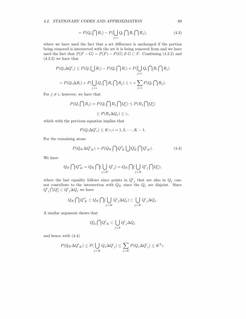
4.2. STATIONARY CODES AND APPROXIMATION 69
= P (Qi
⋂Ri) − P (
⋃j<i
Qi
⋂Ri
⋂Rj), (4.3)
where we have used the fact that a set difference is unchanged if the portionbeing removed is intersected with the set it is being removed from and we haveused the fact that P (F − G) = P (F ) − P (G) if G ⊂ F . Combining (4.2.2) and(4.2.3) we have that
P (Qi∆Q′i) ≤ P (Qi
⋃Ri) − P (Qi
⋂Ri) + P (
⋃j<i
Qi
⋂Ri
⋂Rj)
= P (Qi∆Ri) + P (⋃j<i
Qi
⋂Ri
⋂Rj) ≤ γ +
∑j<i
P (Qi
⋂Rj).
For j 6= i, however, we have that
P (Qi
⋂Rj) = P (Qi
⋂Rj
⋂Qc
j) ≤ P (Rj
⋂Qc
j)
≤ P (Rj∆Qj) ≤ γ,
which with the previous equation implies that
P (Qi∆Q′i) ≤ Kγ; i = 1, 2, · · · ,K − 1.
For the remaining atom:
P (QK∆Q′K) = P (QK
⋂Q′c
K
⋃Qc
K
⋂Q′
K). (4.4)
We have
QK
⋂Q′c
K = QK
⋂(
⋃j<K
Q′j) = QK
⋂(
⋃j<K
Q′j
⋂Qc
j),
where the last equality follows since points in Q′j that are also in Qj can-
not contribute to the intersection with QK since the Qj are disjoint. SinceQ′
j
⋂Qc
j ⊂ Q′j∆Qj we have
QK
⋂Q′c
K ⊂ QK
⋂(
⋃j<K
Q′j∆Qj) ⊂
⋃j<K
Q′j∆Qj .
A similar argument shows that
QcK
⋂Q′
K ⊂⋃j<k
Q′j∆Qj
and hence with (4.4)
P (QK∆Q′K) ≤ P (
⋃j<K
Qj∆Q′j) ≤
∑j<K
P (Qj∆Q′j) ≤ K2γ.
70 CHAPTER 4. INFORMATION RATES I
To summarize, we have shown that
P (Qi∆Q′i) ≤ K2γ; i = 1, 2, · · · ,K
If we now choose γ so small that K2γ ≤ ε/K, the lemma is proved. 2
Corollary 4.2.2: Let (Ω,B, P ) be a probability space and F a generatingfield. Let f : Ω → A be a finite alphabet measurement. Given ε > 0 thereis a measurement g : Ω → A that is measurable with respect to F (that is,g−1(a) ∈ F for all a ∈ A) for which P (f 6= g) ≤ ε.
Proof: Follows from the previous lemma by setting Q = f−1(a); a ∈ A,choosing Q′ from the lemma, and then assigning g for atom Q′
i in Q′ the samevalue that f takes on in atom Qi in Q. Then
P (f 6= g) =12
∑i
P (Qi∆Q′i) ≤ ε. 2
We now develop applications of the previous results which relate the idea ofthe entropy of a dynamical system with the entropy rate of a random process.The result is not required for later coding theorems, but it provides insight intothe connections between entropy as considered in ergodic theory and entropy asused in information theory. In addition, the development involves some ideas ofcoding and approximation which are useful in proving the ergodic theorems ofinformation theory used to prove coding theorems.
Let Xn be a random process with alphabet AX . Let A∞X denote the one or
two-sided sequence space. Consider the dynamical system (Ω,B, P, T ) definedby (A∞
X ,B(AX)∞, P, T ), where P is the process distribution and T the shift.Recall from Section 2.2 that a stationary coding or infinite length sliding blockcoding of Xn is a measurable mapping f : A∞
X → Af into a finite alphabetwhich produces an encoded process fn defined by
fn(x) = f(Tnx); x ∈ A∞X .
The entropy H(P, T ) of the dynamical system was defined by
H(P, T ) = supf
HP (f),
the supremum of the entropy rates of finite alphabet stationary codings of theoriginal process. We shall soon show that if the original alphabet is finite, thenthe entropy of the dynamical system is exactly the entropy rate of the process.First, however, we require several preliminary results, some of independent in-terest.
Lemma 4.2.3: If f is a stationary coding of an AMS process, then theprocess fn is also AMS. If the input process is ergodic, then so is fn.
Proof: Suppose that the input process has alphabet AX and distribution Pand that the measurement f has alphabet Af . Define the sequence mappingf : A∞
X → A∞f by f(x) = fn(x); n ∈ T , where fn(x) = f(Tnx) and T is
4.2. STATIONARY CODES AND APPROXIMATION 71
the shift on the input sequence space A∞X . If T also denotes the shift on the
output space, then by construction f(Tx) = T f(x) and hence for any outputevent F , f−1(T−1F ) = T−1f−1(F ). Let m denote the process distribution forthe encoded process. Since m(F ) = P (f−1(F )) for any event F ∈ B(Af )∞ , wehave using the stationarity of the mapping f that
limn→∞
1n
n−1∑i=0
m(T−iF ) = limn→∞
1n
n−1∑i=0
P (f−1(T−iF ))
= limn→∞
1n
n−1∑i=0
P (T−if−1(F )) = P (f−1(F )),
where P is the stationary mean of P . Thus m is AMS. If G is an invariantoutput event, then f−1(G) is also invariant since T−1f−1(G) = f−1(T−1G).Hence if input invariant sets can only have probability 1 or 0, the same is truefor output invariant sets. 2
The lemma and Theorem 3.1.1 immediately yields the following:Corollary 4.2.3: If f is a stationary coding of an AMS process, then
H(f) = limn→∞
1n
H(fn),
that is, the limit exists.For later use the next result considers general standard alphabets. A sta-
tionary code f is a scalar quantizer if there is a map q : AX → Af such thatf(x) = q(x0). Intuitively, f depends on the input sequence only through thecurrent symbol. Mathematically, f is measurable with respect to σ(X0). Suchcodes are effectively the simplest possible and have no memory or dependenceon the future.
Lemma 4.2.4: Let Xn be an AMS process with standard alphabet AX
and distribution m. Let f be a stationary coding of the process with finitealphabet Af . Fix ε > 0. If the process is two-sided, then there is a scalarquantizer q : AX → Aq, an integer N , and a mapping g : AN
q → Af such that
limn→∞
1n
n−1∑i=0
Pr(fi 6= g(q(Xi−N ), q(Xi−N+1), · · · , q(Xi+N ))) ≤ ε.
If the process is one-sided, then there is a scalar quantizer q : AX → Aq, aninteger N , and a mapping g : AN
q → Af such that
limn→∞
1n
n−1∑i=0
Pr(fi 6= g(q(Xi), q(Xi+1), · · · , q(Xi+N−1))) ≤ ε.
Comment: The lemma states that any stationary coding of an AMS process canbe approximated by a code that depends only on a finite number of quantized
72 CHAPTER 4. INFORMATION RATES I
inputs, that is, by a coding of a finite window of a scalar quantized version ofthe original process. In the special case of a finite alphabet input process, thelemma states that an arbitrary stationary coding can be well approximated bya coding depending only on a finite number of the input symbols.
Proof: Suppose that m is the stationary mean and hence for any measure-ments f and g
m(f0 6= g0) = limn→∞
1n
n−1∑n=0
Pr(fi 6= gi).
Let qn be an asymptotically accurate scalar quantizer in the sense that σ(qn(X0))asymptotically generates B(AX). (Since AX is standard this exists. If AX isfinite, then take q(a) = a.) Then Fn = σ(qn(Xi); i = 0, 1, 2, · · · , n − 1) asymp-totically generates B(AX)∞ for one-sided processes and Fn = σ(qn(Xi); i =−n, · · · , n) does the same for two-sided processes. Hence from Corollary 4.2.2given ε we can find a sufficiently large n and a mapping g that is measurablewith respect to Fn such that m(f 6= g) ≤ ε. Since g is measurable with respectto Fn, it must depend on only the finite number of quantized samples thatgenerate Fn. (See, e.g., Lemma 5.2.1 of [50].) This proves the lemma. 2
Combining the lemma and Corollary 4.2.1 immediately yields the followingcorollary, which permits us to study the entropy rate of general stationary codesby considering codes which depend on only a finite number of inputs (and hencefor which the ordinary entropy results for random vectors can be applied).
Corollary 4.2.4: Given a stationary coding f of an AMS process let Fn bedefined as above. Then given ε > 0 there exists for sufficiently large n a code gmeasurable with respect to Fn such that
|H(f) − H(g)| ≤ ε.
The above corollary can be used to show that entropy rate, like entropy,is reduced by coding. The general stationary code is approximated by a codedepending on only a finite number of inputs and then the result that entropy isreduced by mapping (Lemma 2.3.3) is applied.
Corollary 4.2.5: Given an AMS process Xn with finite alphabet AX anda stationary coding f of the process, then
H(X) ≥ H(f),
that is, stationary coding reduces entropy rate.Proof: For integer n define Fn = σ(X0, X1, · · · , Xn) in the one-sided case
and σ(X−n, · · · , Xn) in the two-sided case. Then Fn asymptotically generatesB(AX)∞. Hence given a code f and an ε > 0 we can choose using the finitealphabet special case of the previous lemma a large k and a Fk-measurable codeg such that |H(f) − H(g)| ≤ ε. We shall show that H(g) ≤ H(X), which willprove the lemma. To see this in the one-sided case observe that g is a functionof Xk and hence gn depends only on Xn+k and hence
H(gn) ≤ H(Xn+k)
4.3. INFORMATION RATE OF FINITE ALPHABET PROCESSES 73
and hence
H(g) = limn→∞
1n
H(gn) ≤ limn→∞
1n
n
n + kH(Xn+k) = H(X).
In the two-sided case g depends on X−k, · · · , Xk and hence gn depends onX−k, · · · , Xn+k and hence
H(gn) ≤ H(X−k, · · · , X−1, X0, · · · , Xn+k) ≤ H(X−k, · · · , X−1) + H(Xn+k).
Dividing by n and taking the limit completes the proof as before. 2
Theorem 4.2.1: Let Xn be a random process with alphabet AX . LetA∞
X denote the one or two-sided sequence space. Consider the dynamical system(Ω,B, P, T ) defined by (A∞
X ,B(AX)∞, P, T ), where P is the process distributionand T is the shift. Then
H(P, T ) = H(X).
Proof: From (2.2.4), H(P, T ) ≥ H(X). Conversely suppose that f is a codewhich yields H(f) ≥ H(P, T ) − ε. Since f is a stationary coding of the processXn, the previous corollary implies that H(f) ≤ H(X), which completes theproof. 2
4.3 Information Rate of Finite Alphabet Pro-cesses
Let (Xn, Yn) be a one-sided random process with finite alphabet A × B andlet ((A×B)Z+ ,B(A×B)Z+) be the corresponding one-sided sequence space ofoutputs of the pair process. We consider Xn and Yn to be the sampling functionson the sequence spaces A∞ and B∞ and (Xn, Yn) to be the pair samplingfunction on the product space, that is, for (x, y) ∈ A∞ × B∞, (Xn, Yn)(x, y)= (Xn(x), Yn(y)) = (xn, yn). Let p denote the process distribution induced bythe original space on the process (Xn, Yn). Analogous to entropy rate wecan define the mutual information rate (or simply information rate) of a finitealphabet pair process by
I(X,Y ) = lim supn→∞
1n
I(Xn, Y n).
The following lemma follows immediately from the properties of entropy ratesof Theorems 2.4.1 and 3.1.1 since for AMS finite alphabet processes
I(X;Y ) = H(X) + H(Y ) − H(X,Y )
and since from (3.1.4) the entropy rate of an AMS process is the same as that ofits stationary mean. Analogous to Theorem 3.1.1 we define the random variablesp(Xn, Y n) by p(Xn, Y n)(x, y) = p(Xn = xn, Y n = yn), p(Xn) by p(Xn)(x, y)= p(Xn = xn), and similarly for p(Y n).
74 CHAPTER 4. INFORMATION RATES I
Lemma 4.3.1: Suppose that Xn, Yn is an AMS finite alphabet randomprocess with distribution p and stationary mean p. Then the limits supremumdefining information rates are limits and
Ip(X,Y ) = Ip(X,Y ).
Ip is an affine function of the distribution p. If p has ergodic decomposition pxy,then
Ip(X,Y ) =∫
dp(x, y)Ipxy(X,Y ).
If we define the information density
in(Xn, Y n) = lnp(Xn, Y n)
p(Xn)p(Y n),
thenlim
n→∞
1n
in(Xn, Y n) = Ipxy(X,Y )
almost everywhere with respect to p and p and in L1(p).The following lemmas follow either directly from or similarly to the corre-
sponding results for entropy rate of the previous section.Lemma 4.3.2: Suppose that Xn, Yn, X ′
n, Y ′n is an AMS process and
P = limn→∞
1n
n−1∑i=0
Pr((Xi, Yi) 6= (X ′i, Y
′i)) ≤ ε
(the limit exists since the process is AMS). Then
|I(X;Y ) − I(X ′;Y ′)| ≤ 3(ε ln(||A|| − 1) + h2(ε)).
Proof: The inequality follows from Corollary 4.2.1 since
|(X;Y ) − I(X ′;Y ′)| ≤
|H(X) − H(X ′)| + |H(Y ) − H(Y ′)| + |H(X,Y ) − H(X ′, Y ′)|and since Pr((Xi, Yi) 6= (Xi
′, Yi′)) = Pr(Xi 6= Xi
′ or Yi 6= Yi′) is no smaller
than Pr(Xi 6= Xi′) or Pr(Yi 6= Yi
′). 2
Corollary 4.3.1: Let Xn, Yn be an AMS process and let f and g bestationary measurements on X and Y , respectively. Given ε > 0 there is anN sufficiently large, scalar quantizers q and r, and mappings f ′ and g′ whichdepend only on q(X0), · · · , q(XN−1) and r(Y0), · · · , r(YN−1) in the one-sidedcase and q(X−N ), · · · , q(XN ) and r(Y−N ), · · · , r(YN ) in the two-sided casesuch that
|I(f ; g) − I(f ′; g′)| ≤ ε.
Proof: Choose the codes f ′ and g′ from Lemma 4.2.4 and apply the previouslemma. 2

4.3. INFORMATION RATE OF FINITE ALPHABET PROCESSES 75
Lemma 4.3.3:If Xn, Yn is an AMS process and f and g are stationarycodings of X and Y , respectively, then
I(X;Y ) ≥ I(f ; g).
Proof: This is proved as Corollary 4.2.5 by first approximating f and g by finite-window stationary codes, applying the result for mutual information (Lemma2.5.2), and then taking the limit. 2

76 CHAPTER 4. INFORMATION RATES I
Chapter 5
Relative Entropy
5.1 Introduction
A variety of information measures have been introduced for finite alphabet ran-dom variables, vectors, and processes:entropy, mutual information, relative en-tropy, conditional entropy, and conditional mutual information. All of thesecan be expressed in terms of divergence and hence the generalization of thesedefinitions to infinite alphabets will follow from a general definition of diver-gence. Many of the properties of generalized information measures will thenfollow from those of generalized divergence.
In this chapter we extend the definition and develop the basic propertiesof divergence, including the formulas for evaluating divergence as expectationsof information densities and as limits of divergences of finite codings. We alsodevelop several inequalities for and asymptotic properties of divergence. Theseresults provide the groundwork needed for generalizing the ergodic theorems ofinformation theory from finite to standard alphabets. The general definitionsof entropy and information measures originated in the pioneering work of Kol-mogorov and his colleagues Gelfand, Yaglom, Dobrushin, and Pinsker [45] [90][32] [125].
5.2 Divergence
Given a probability space (Ω,B, P ) (not necessarily with finite alphabet) andanother probability measure M on the same space, define the divergence of Pwith respect to M by
D(P ||M) = supQ
HP ||M (Q) = supf
D(Pf ||Mf ), (5.1)
where the first supremum is over all finite measurable partitions Q of Ω and thesecond is over all finite alphabet measurements on Ω. The two forms have thesame interpretation: the divergence is the supremum of the relative entropies
77
78 CHAPTER 5. RELATIVE ENTROPY
or divergences obtainable by finite alphabet codings of the sample space. Thepartition form is perhaps more common when considering divergence per se,but the measurement or code form is usually more intuitive when consideringentropy and information. This section is devoted to developing the basic proper-ties of divergence, all of which will yield immediate corollaries for the measuresof information.
The first result is a generalization of the divergence inequality that is a trivialconsequence of the definition and the finite alphabet special case.
Lemma 5.2.1: The Divergence Inequality:For any two probability measures P and M
D(P ||M) ≥ 0
with equality if and only if P = M .Proof: Given any partition Q, Theorem 2.3.1 implies that
∑Q∈Q
P (Q) lnP (Q)M(Q)
≥ 0
with equality if and only if P (Q) = M(Q) for all atoms Q of the partition. SinceD(P ||Q) is the supremum over all such partitions, it is also nonnegative. It canbe 0 only if P and M assign the same probabilities to all atoms in all partitions(the supremum is 0 only if the above sum is 0 for all partitions) and hence thedivergence is 0 only if the measures are identical. 2
As in the finite alphabet case, Lemma 5.2.1 justifies interpreting divergenceas a form of distance or dissimilarity between two probability measures. It isnot a true distance or metric in the mathematical sense since it is not symmetricand it does not satisfy the triangle inequality. Since it is nonnegative and equalszero only if two measures are identical, the divergence is a distortion measureas considered in information theory [51], which is a generalization of the notionof distance. This view often provides interpretations of the basic properties ofdivergence. We shall develop several relations between the divergence and otherdistance measures. The reader is referred to Csiszar [25] for a development ofthe distance-like properties of divergence.
The following two lemmas provide means for computing divergences andstudying their behavior. The first result shows that the supremum can be con-fined to partitions with atoms in a generating field. This will provide a meansfor computing divergences by approximation or limits. The result is due toDobrushin and is referred to as Dobrushin’s theorem. The second result showsthat the divergence can be evaluated as the expectation of an entropy densitydefined as the logarithm of the Radon-Nikodym derivative of one measure rela-tive to the other. This result is due to Gelfand, Yaglom, and Perez. The proofslargely follow the translator’s remarks in Chapter 2 of Pinsker [125] (which inturn follows Dobrushin [32]).
Lemma 5.2.2: Suppose that (Ω,B) is a measurable space where B is gen-erated by a field F , B = σ(F). Then if P and M are two probability measures
5.2. DIVERGENCE 79
on this space,D(P ||M) = sup
Q⊂FHP ||M (Q).
Proof: From the definition of divergence, the right-hand term above is clearlyless than or equal to the divergence. If P is not absolutely continuous withrespect to M , then we can find a set F such that M(F ) = 0 but P (F ) 6= 0 andhence the divergence is infinite. Approximating this event by a field element F0
by applying Theorem 1.2.1 simultaneously to M and G will yield a partitionF0, F
c0 for which the right hand side of the previous equation is arbitrarily
large. Hence the lemma holds for this case. Henceforth assume that M >> P .Fix ε > 0 and suppose that a partition Q = Q1, · · · , QK yields a relative
entropy close to the divergence, that is,
HP ||M (Q) =K∑
i=1
P (Qi) lnP (Qi)M(Qi)
≥ D(P ||M) − ε/2.
We will show that there is a partition, say Q′ with atoms in F which hasalmost the same relative entropy, which will prove the lemma. First observe thatP (Q) ln[P (Q)/M(Q)] is a continuous function of P (Q) and M(Q) in the sensethat given ε/(2K) there is a sufficiently small δ > 0 such that if |P (Q)−P (Q′)| ≤δ and |M(Q) − M(Q′)| ≤ δ, then provided M(Q) 6= 0
|P (Q) lnP (Q)M(Q)
− P (Q′) lnP (Q′)M(Q′)
| ≤ ε
2K.
If we can find a partition Q′ with atoms in F such that
|P (Q′i) − P (Qi)| ≤ δ, |M(Q′
i) − M(Qi)| ≤ δ, i = 1, · · · ,K, (5.2)
then
|HP ||M (Q′) − HP ||M (Q)| ≤∑
i
|P (Qi) lnP (Qi)M(Qi)
− P (Q′i) ln
P (Q′i)
M(Q′i)|
≤ Kε
2K=
ε
2and hence
HP ||M (Q′) ≥ D(P ||M) − ε
which will prove the lemma. To find the partition Q′ satisfying (5.2), let m bethe mixture measure P/2+M/2. As in the proof of Lemma 4.2.2, we can find apartition Q′ ⊂ F such that m(Qi∆Q′
i) ≤ K2γ for i = 1, 2, · · · ,K, which impliesthat
P (Qi∆Q′i) ≤ 2K2γ; i = 1, 2, · · · ,K,
andM(Qi∆Q′
i) ≤ 2K2γ; i = 1, 2, · · · ,K.
80 CHAPTER 5. RELATIVE ENTROPY
If we now choose γ so small that 2K2γ ≤ δ, then (5.2.2) and hence the lemmafollow from the above and the fact that
|P (F ) − P (G)| ≤ P (F∆G).2 (5.3)
Lemma 5.2.3: Given two probability measures P and M on a commonmeasurable space (Ω,B), if P is not absolutely continuous with respect to M ,then
D(P ||M) = ∞.
If P << M (e.g., if D(P ||M) < ∞), then the Radon-Nikodym derivative f =dP/dM exists and
D(P ||M) =∫
ln f(ω)dP (ω) =∫
f(ω) ln f(ω)dM(ω).
The quantity ln f (if it exists) is called the entropy density or relative entropydensity of P with respect to M .
Proof: The first statement was shown in the proof of the previous lemma. IfP is not absolutely continuous with respect to M , then there is a set Q such thatM(Q) = 0 and P (Q) > 0. The relative entropy for the partition Q = Q,Qcis then infinite, and hence so is the divergence.
Assume that P << M and let f = dP/dM . Suppose that Q is an event forwhich M(Q) > 0 and consider the conditional cumulative distribution functionfor the real random variable f given that ω ∈ Q:
FQ(u) =M(f < u
⋂Q)
M(Q);u ∈ (−∞,∞).
Observe that the expectation with respect to this distribution is
EM (f |Q) =∫ ∞
0
u dFQ(u) =1
M(Q)
∫Q
f(ω) dM(ω) =P (Q)M(Q)
.
We also have that∫ ∞
0
u lnu dFQ(u) =1
M(Q)
∫Q
f(ω) ln f(ω) dM(ω),
where the existence of the integral is ensured by the fact that u lnu ≥ −e−1.Applying Jensen’s inequality to the convex
⋃function u lnu yields the in-
equality
1M(Q)
∫Q
ln f(ω) dP (ω) =1
M(Q)
∫Q
f(ω) ln f(ω) dM(ω) =∫ ∞
0
u lnu dFQ(u)
≥ [∫ ∞
0
u dFQ(u)] ln[∫ ∞
0
u dFQ(u)] =P (Q)M(Q)
lnP (Q)M(Q)
.
5.2. DIVERGENCE 81
We therefore have that for any event Q with M(Q) > 0 that∫Q
ln f(ω) dP (ω) ≥ P (Q) lnP (Q)M(Q)
. (5.4)
Now let Q = Qi be a finite partition and we have∫ln f(ω)dP (ω) =
∑i
∫Qi
ln f(ω) dP (ω)
≥∑
i:P (Qi) 6=0
∫Qi
ln f(ω) dP (ω) =∑
i
P (Qi) lnP (Qi)M(Qi)
,
where the inequality follows from (5.2.4) since P (Qi) 6= 0 implies that M(Qi) 6=0 since M >> P . This proves that
D(P ||M) ≤∫
ln f(ω) dP (ω).
To obtain the converse inequality, let qn denote the asymptotically accuratequantizers of Section 1.6. From (1.6.3)∫
ln f(ω) dP (ω) = limn→∞
∫qn(ln f(ω)) dP (ω).
For fixed n the quantizer qn induces a partition of Ω into 2n2n + 1 atomsQ. In particular, there are 2n2n − 1 “good” atoms such that for ω, ω′ insidethe atoms we have that | ln f(ω) − ln f(ω′)| ≤ 2−(n−1). The remaining twoatoms group ω for which ln f(ω) ≥ n or ln f(ω) < −n. Defining the shorthandP (ln f < −n) = P (ω : ln f(ω) < −n), we have then that
∑Q∈Q
P (Q) lnP (Q)M(Q)
=∑
good Q
P (Q) lnP (Q)M(Q)
+P (ln f ≥ n) lnP (ln f ≥ n)M(ln f ≥ n)
+ P (ln f < −n) lnP (ln f < −n)M(ln f < −n)
.
The rightmost two terms above are bounded below as
P (ln f ≥ n) lnP (ln f ≥ n)M(ln f ≥ n)
+ P (ln f < −n) lnP (ln f < −n)M(ln f < −n)
≥ P (ln f ≥ n) ln P (ln f ≥ n) + P (ln f < −n) ln P (ln f < −n).
Since P (ln f ≥ n) and P (ln f < −n) → 0 as n → ∞ and since x lnx → 0 asx → 0, given ε we can choose n large enough to ensure that the above term isgreater than −ε. This yields the lower bound
∑Q∈Q
P (Q) lnP (Q)M(Q)
≥∑
good Q
P (Q) lnP (Q)M(Q)
− ε.
82 CHAPTER 5. RELATIVE ENTROPY
Fix a good atom Q and define h = supω∈Q ln f(ω) and h = infω∈Q ln f(ω)and note that by definition of the good atoms
h − h ≤ 2−(n−1).
We now have that
P (Q)h ≥∫
Q
ln f(ω) dP (ω)
and
M(Q)eh ≤∫
Q
f(ω)dM(ω) = P (Q).
Combining these we have that
P (Q) lnP (Q)M(Q)
≥ P (Q) lnP (Q)
P (Q)e−h= P (Q)h
≥ P (Q)(h − 2−(n−1)) ≥∫
Q
ln f(ω)dP (ω) − P (Q)2−(n−1).
Therefore ∑Q∈Q
P (Q) lnP (Q)M(Q)
≥∑
good Q
P (Q) lnP (Q)M(Q)
− ε
≥∑
good Q
∫Q
ln f(ω) dP − 2−(n−1) − ε
=∫
ω:| ln f(ω)|≤n
ln f(ω) dP (ω) − 2−(n−1) − ε.
Since this is true for arbitrarily large n and arbitrarily small ε,
D(P ||Q) ≥∫
ln f(ω)dP (ω),
completing the proof of the lemma. 2
It is worthwhile to point out two examples for the previous lemma. If P andM are discrete measures with corresponding pmf’s p and q, than the Radon-Nikodym derivative is simply dP/dM(ω) = p(ω)/m(ω) and the lemma gives theknown formula for the discrete case. If P and M are both probability measureson Euclidean space Rn and if both measures are absolutely continuous withrespect to Lebesgue measure, then there exists a density f called a probabilitydensity function or pdf such that
P (F ) =∫
F
f(x)dx,
5.2. DIVERGENCE 83
where dx means dm(x) with m Lebesgue measure. (Lebesgue measure assignseach set its volume.) Similarly, there is a pdf g for M . In this case,
D(P ||M) =∫Rn
f(x) lnf(x)g(x)
dx. (5.5)
The following immediate corollary to the previous lemma provides a formulathat is occasionally useful for computing divergences.
Corollary 5.2.1: Given three probability distributions M >> Q >> P ,then
D(P ||M) = D(P ||Q) + EP (lndQ
dM).
Proof: From the chain rule for Radon-Nikodym derivatives (e.g., Lemma5.7.3 of [50])
dP
dM=
dP
dQ
dQ
dM
and taking expectations using the previous lemma yields the corollary. 2
The next result is a technical result that shows that given a mapping ona space, the divergence between the induced distributions can be computedfrom the restrictions of the original measures to the sub-σ-field induced bythe mapping. As part of the result, the relation between the induced Radon-Nikodym derivative and the original derivative is made explicit.
Recall that if P is a probability measure on a measurable space (Ω,B) andif F is a sub-σ-field of B, then the restriction PF of P to F is the probabilitymeasure on the measurable space (Ω,F) defined by PF (G) = P (G), for allG ∈ F . In other words, we can use either the probability measures on the newspace or the restrictions of the probability measures on the old space to computethe divergence. This motivates considering the properties of divergences ofrestrictions of measures, a useful generality in that it simplifies proofs. Thefollowing lemma can be viewed as a bookkeeping result relating the divergenceand the Radon-Nikodym derivatives in the two spaces.
Lemma 5.2.4: (a) Suppose that M,P are two probability measures ona space (Ω,B) and that X is a measurement mapping this space into (A,A).Let PX and MX denote the induced distributions (measures on (A,A)) and letPσ(X) and Mσ(X) denote the restrictions of P and M to σ(X), the sub-σ-fieldof B generated by X. Then
D(PX ||MX) = D(Pσ(X)||Mσ(X)).
If the Radon-Nikodym derivative f = dPX/dMX exists (e.g., the above diver-gence is finite), then define the function f(X) : Ω → [0,∞) by
f(X)(ω) = f(X(ω)) =dPX
dMX(X(ω));
then with probability 1 under both M and P
f(X) =dPσ(X)
dMσ(X).
84 CHAPTER 5. RELATIVE ENTROPY
(b) Suppose that P << M . Then for any sub-σ-field F of B, we have that
dPFdMF
= EM (dP
dM|F).
Thus the Radon-Nikodym derivative for the restrictions is just the conditionalexpectation of the original Radon-Nikodym derivative.
Proof: The proof is mostly algebra: D(Pσ(X)||Mσ(X)) is the supremum overall finite partitions Q with elements in σ(X) of the relative entropy HPσ(X)||Mσ(X)
(Q).Each element Q ∈ Q ⊂ σ(X) corresponds to a unique set Q′ ∈ A via Q =X−1(Q′) and hence to each Q ⊂ σ(X) there is a corresponding partition Q′ ⊂ A.The corresponding relative entropies are equal, however, since
HPX ||MX(Q′) =
∑Q′∈Q′
Pf (Q′) lnPX(Q′)MX(Q′)
=∑
Q′∈Q′
P (X−1(Q′)) lnP (X−1(Q′))M(X−1(Q′))
=∑Q∈Q
PX(Q) lnPX(Q)MX(Q)
= HPσ(X)||Mσ(X)(Q).
Taking the supremum over the partitions proves that the divergences are equal.If the derivative is f = dPX/dMX , then f(X) is measurable since it is a mea-surable function of a measurable function. In addition, it is measurable withrespect to σ(X) since it depends on ω only through X(ω). For any F ∈ σ(X)there is a G ∈ A such that F = X−1(G) and∫
F
f(X)dMσ(X) =∫
F
f(X)dM =∫
G
fdMX
from the change of variables formula (see, e.g., Lemma 4.4.7 of [50]). Thus∫F
f(X)dMσ(X) = PX(G) = Pσ(X)(X−1(G)) = Pσ(X)(F ),
which proves that f(X) is indeed the claimed derivative with probability 1 underM and hence also under P .
The variation quoted in part (b) is proved by direct verification using iteratedexpectation. If G ∈ F , then using iterated expectation we have that∫
G
EM (dP
dM|F) dMF =
∫EM (1G
dP
dM|F) dMF
Since the argument of the integrand is F-measurable (see, e.g., Lemma 5.3.1 of[50]), invoking iterated expectation (e.g., Corollary 5.9.3 of [50]) yields∫
G
EM (dP
dM|F) dMF =
∫EM (1G
dP
dM|F) dM
5.2. DIVERGENCE 85
= E(1GdP
dM) = P (G) = PF (G),
proving that the conditional expectation is the claimed derivative. 2
Part (b) of the Lemma was pointed out to the author by Paul Algoet.Having argued above that restrictions of measures are useful when finding
divergences of random variables, we provide a key trick for treating such restric-tions.
Lemma 5.2.5: Let M >> P be two measures on a space (Ω,B). Supposethat F is a sub-σ-field and that PF and MF are the restrictions of P and M toF Then there is a measure S such that M >> S >> P and
dP
dS=
dP/dM
dPF/dMF,
dS
dM=
dPFdMF
,
andD(P ||S) + D(PF ||MF ) = D(P ||M). (5.6)
Proof: If M >> P , then clearly MF >> PF and hence the appropriateRadon-Nikodym derivatives exist. Define the set function S by
S(F ) =∫
F
dPFdMF
dM =∫
F
EM (dP
dM|F) dM,
using part (b) of the previous lemma. Thus M >> S and dS/dM = dPF/dMF .Observe that for F ∈ F , iterated expectation implies that
S(F ) = EM (EM (1FdP
dM|F)) = EM (1F
dP
dM)
= P (F ) = PF (F ); F ∈ Fand hence in particular that S(Ω) is 1 so that dPF/dMF is integrable and S isindeed a probability measure on (Ω,B). (In addition, the restriction of S to Fis just PF .) Define
g =dP/dM
dPF/dMF.
This is well defined since with M probability 1, if the denominator is 0, thenso is the numerator. Given F ∈ B the Radon-Nikodym theorem (e.g., Theorem5.6.1 of [50]) implies that∫
F
gdS =∫
1F gdS
dMdM =
∫1F
dP/dM
dPF/dMFdPF/dMFdM = P (F ),
that is, P << S anddP
dS=
dP/dM
dPF/dMF,
86 CHAPTER 5. RELATIVE ENTROPY
proving the first part of the lemma. The second part follows by direct verifica-tion:
D(P ||M) =∫
lndP
dMdP =
∫ln
dPFdMF
dP +∫
lndP/dM
dPF/dMFdP
=∫
lndPFdMF
dPF +∫
lndP
dSdP = D(PF ||MF ) + D(P ||S). 2
The two previous lemmas and the divergence inequality immediately yieldthe following result for M >> P . If M does not dominate P , then the result istrivial.
Corollary 5.2.2: Given two measures M,P on a space (Ω,B) and a sub-σ-field F of B, then
D(P ||M) ≥ D(PF ||MF ).
If f is a measurement on the given space, then
D(P ||M) ≥ D(Pf ||Mf ).
The result is obvious for finite fields F or finite alphabet measurements ffrom the definition of divergence. The general result for arbitrary measurablefunctions could also have been proved by combining the corresponding finitealphabet result of Corollary 2.3.1 and an approximation technique. As above,however, we will occasionally get results comparing the divergences of measuresand their restrictions by combining the trick of Lemma 5.2.5 with a result for asingle divergence.
The following corollary follows immediately from Lemma 5.2.2 since theunion of a sequence of asymptotically generating sub-σ-fields is a generatingfield.
Corollary 5.2.3: Suppose that M,P are probability measures on a mea-surable space (Ω,B) and that Fn is an asymptotically generating sequence ofsub-σ-fields and let Pn and Mn denote the restrictions of P and M to Fn (e.g.,Pn = PFn
). ThenD(Pn||Mn) ↑ D(P ||M).
There are two useful special cases of the above corollary which follow im-mediately by specifying a particular sequence of increasing sub-σ-fields. Thefollowing two corollaries give these results.
Corollary 5.2.4: Let M,P be two probability measures on a measurablespace (Ω,B). Suppose that f is an A-valued measurement on the space. Assumethat qn : A → An is a sequence of measurable mappings into finite sets An withthe property that the sequence of fields Fn = F(qn(f)) generated by the setsq−1
n (a); a ∈ An asymptotically generate σ(f). (For example, if the originalspace is standard let Fn be a basis and let qn map the points in the ith atomof Fn into i.) Then
D(Pf ||Mf ) = limn→∞
D(Pqn(f)||Mqn(f)).
5.2. DIVERGENCE 87
The corollary states that the divergence between two distributions of a ran-dom variable can be found as a limit of quantized versions of the random vari-able. Note that the limit could also be written as
limn→∞
HPf ||Mf(qn).
In the next corollary we consider increasing sequences of random variablesinstead of increasing sequences of quantizers, that is, more random variables(which need not be finite alphabet) instead of ever finer quantizers. The corol-lary follows immediately from Corollary 5.2.3 and Lemma 5.2.4.
Corollary 5.2.5: Suppose that M and P are measures on the sequencespace corresponding to outcomes of a sequence of random variables X0, X1, · · ·with alphabet A. Let Fn = σ(X0, · · · , Xn−1), which asymptotically generatesthe σ-field σ(X0, X1, · · ·). Then
limn→∞
D(PXn ||MXn) = D(P ||M).
We now develop two fundamental inequalities involving entropy densitiesand divergence. The first inequality is from Pinsker [125]. The second is animprovement of an inequality of Pinsker [125] by Csiszar [24] and Kullback [91].The second inequality is more useful when the divergence is small. Couplingthese inequalities with the trick of Lemma 5.2.5 provides a simple generalizationof an inequality of [48] and will provide easy proofs of L1 convergence resultsfor entropy and information densities. A key step in the proof involves a notionof distance between probability measures and is of interest in its own right.Given two probability measures M,P on a common measurable space (Ω,B),the variational distance between them is defined by
d(P,M) ≡ supQ
∑Q∈Q
|P (Q) − M(Q)|,
where the supremum is over all finite measurable partitions. We will proceed bystating first the end goal, the two inequalities involving divergence, as a lemma,and then state two lemmas giving the basic required properties of the variationaldistance. The lemmas will be proved in a different order.
Lemma 5.2.6: Let P and M be two measures on a common probabilityspace (Ω,B) with P << M . Let f = dP/dM be the Radon-Nikodym derivativeand let h = ln f be the entropy density. Then
D(P ||M) ≤∫
|h|dP ≤ D(P ||M) +2e, (5.7)
∫|h|dP ≤ D(P ||M) +
√2D(P ||M). (5.8)
Lemma 5.2.7: Given two probability measures M,P on a common mea-surable space (Ω,B), the variational distance is given by
d(P,M) = 2 supF∈B
|P (F ) − M(F )|. (5.9)
88 CHAPTER 5. RELATIVE ENTROPY
Furthermore, if S is a measure for which P << S and M << S (S = (P +M)/2,for example), then also
d(P,M) =∫
|dP
dS− dM
dS| dS (5.10)
and the supremum in (5.9) is achieved by the set
F = ω :dP
dS(ω) >
dM
dS(ω).
Lemma 5.2.8
d(P,M) ≤√
2D(P ||M).
Proof of Lemma 5.2.7: First observe that for any set F we have for thepartition Q = F, F c that
d(P,M) ≥∑Q∈Q
|P (Q) − M(Q)| = 2|P (F ) − M(F )|
and henced(P,M) ≥ 2 sup
F∈B|P (F ) − M(F )|.
Conversely, suppose that Q is a partition which approximately yields the vari-ational distance, e.g., ∑
Q∈Q|P (Q) − M(Q)| ≥ d(P,M) − ε
for ε > 0. Define a set F as the union of all of the Q in Q for which P (Q) ≥ M(Q)and we have that∑
Q∈Q|P (Q) − M(Q)| = P (F ) − M(F ) + M(F c) − P (F c) = 2(P (F ) − M(F ))
and henced(P,M) − ε ≤ sup
F∈B2|P (F ) − M(F )|.
Since ε is arbitrary, this proves the first statement of the lemma.Next suppose that a measure S dominating both P and M exists and define
the setF = ω :
dP
dS(ω) >
dM
dS(ω)
and observe that∫|dP
dS− dM
dS| dS =
∫F
(dP
dS− dM
dS) dS −
∫F c
(dP
dS− dM
dS) dS
5.2. DIVERGENCE 89
= P (F ) − M(F ) − (P (F c) − M(F c)) = 2(P (F ) − M(F )).
From the definition of F , however,
P (F ) =∫
F
dP
dSdS ≥
∫F
dM
dSdS = M(F )
so that P (F ) − M(F ) = |P (F ) − M(F )|. Thus we have that∫|dP
dS− dM
dS| dS = 2|P (F ) − M(F )| ≤ 2 sup
G∈B|P (G) − M(G)| = d(P,M).
To prove the reverse inequality, assume that Q approximately yields the varia-tional distance, that is, for ε > 0 we have∑
Q∈Q|P (Q) − M(Q)| ≥ d(P,M) − ε.
Then ∑Q∈Q
|P (Q) − M(Q)| =∑Q∈Q
|∫
Q
(dP
dS− dM
dS) dS|
≤∑Q∈Q
∫Q
|dP
dS− dM
dS| dS =
∫|dP
dS− dM
dS| dS
which, since ε is arbitrary, proves that
d(P,M) ≤∫
|dP
dS− dM
dS| dS,
Combining this with the earlier inequality proves (5.10). We have already seenthat this upper bound is actually achieved with the given choice of F , whichcompletes the proof of the lemma. 2
Proof of Lemma 5.2.8: Assume that M >> P since the result is trivialotherwise because the right-hand side is infinite. The inequality will followfrom the first statement of Lemma 5.2.7 and the following inequality: Given1 ≥ p,m ≥ 0,
p lnp
m+ (1 − p) ln
1 − p
1 − m− 2(p − m)2 ≥ 0. (5.11)
To see this, suppose the truth of (5.11). Since F can be chosen so that 2(P (F )−M(F )) is arbitrarily close to d(P,M), given ε > 0 choose a set F such that[2(P (F ) − M(F ))]2 ≥ d(P,M)2 − 2ε. Since F, F c is a partition,
D(P ||M) − d(P,M)2
2
≥ P (F ) lnP (F )M(F )
+ (1 − P (F )) ln1 − P (F )1 − M(F )
− 2(P (F ) − M(F ))2 − ε.
90 CHAPTER 5. RELATIVE ENTROPY
If (5.11) holds, then the right-hand side is bounded below by −ε, which provesthe lemma since ε is arbitrarily small. To prove (5.11) observe that the left-hand side equals zero for p = m, has a negative derivative with respect to mfor m < p, and has a positive derivative with respect to m for m > p. (Thederivative with respect to m is (m − p)[1 − 4m(1 − m)]/[m(1 − m).) Thus theleft hand side of (5.11) decreases to its minimum value of 0 as m tends to p fromabove or below. 2
Proof of Lemma 5.2.6: The magnitude entropy density can be written as
|h(ω)| = h(ω) + 2h(ω)− (5.12)
where a− = −min(a, 0). This inequality immediately gives the trivial left-handinequality of (5.7). The right-hand inequality follows from the fact that∫
h−dP =∫
f [ln f ]−dM
and the elementary inequality a ln a ≥ −1/e.The second inequality will follow from (5.12) if we can show that
2∫
h−dP ≤√
2D(P ||M).
Let F denote the set h ≤ 0 and we have from (5.4) that
2∫
h−dP = −2∫
F
hdP ≤ −2P (F ) lnP (F )M(F )
and hence using the inequality lnx ≤ x − 1 and Lemma 5.2.7
2∫
h−dP ≤ 2P (F ) lnM(F )P (F )
≤ 2(M(F ) − P (F ))
≤ d(P,M) ≤√
2D(P ||M),
completing the proof. 2
Combining Lemmas 5.2.6 and 5.2.5 yields the following corollary, which gen-eralizes Lemma 2 of [54]:
Corollary 5.2.6: Let P and M be two measures on a space (Ω,B). Supposethat F is a sub-σ-field and that PF and MF are the restrictions of P and Mto F . Assume that M >> P . Define the entropy densities h = ln dP/dM andh′ = ln dPF/dMF . Then∫
|h − h′| dP ≤ D(P ||M) − D(PF ||MF ) +2e, (5.13)
and ∫|h − h′| dP ≤ D(P ||M)−
D(PF ||MF ) +√
2D(P ||M) − 2D(PF ||MF ). (5.14)
Proof: Choose the measure S as in Lemma 5.2.5 and then apply Lemma5.2.6 with S replacing M . 2
5.2. DIVERGENCE 91
Variational Description of Divergence
As in the discrete case, divergence has a variational characterization that is afundamental property for its applications to large deviations theory [143] [31].We again take a detour to state and prove the property without delving into itsapplications.
Suppose now that P and M are two probability measures on a commonprobability space, say (Ω,B), such that M >> P and hence the density
f =dP
dM
is well defined. Suppose that Φ is a real-valued random variable defined on thesame space, which we explicitly require to be finite-valued (it cannot assume ∞as a value) and to have finite cumulant generating function:
EM (eΦ) < ∞.
Then we can define a probability measure Mφ by
MΦ(F ) =∫
F
eΦ
EM (eΦ)dM (5.15)
and observe immediately that by construction M >> MΦ and
dMΦ
dM=
eΦ
EM (eΦ).
The measure MΦ is called a “tilted” distribution. Furthermore, by constructiondMΦ/dM 6= 0 and hence we can write∫
F
f
eφ/EM (eΦ)dQ =
∫F
f
eφ/EM (eΦ)dMΦ
dMdM =
∫F
fdM = P (F )
and hence P << MΦ and
dP
dMΦ=
f
eφ/EM (eΦ).
We are now ready to state and prove the principal result of this section, avariational characterization of divergence.
Theorem 5.2.1: Suppose that M >> P . Then
D(P ||M) = supΦ
(EP Φ − ln(EM (eΦ))
), (5.16)
where the supremum is over all random variables Φ for which Φ is finite-valuedand eΦ is M -integrable.
Proof: First consider the random variable Φ defined by Φ = ln f and observethat
EP Φ − ln(EM (eΦ)) =∫
dP ln f − ln(∫
dMf)
92 CHAPTER 5. RELATIVE ENTROPY
= D(P ||M) − ln∫
dP = D(P ||M).
This proves that the supremum over all Φ is no smaller than the divergence. Toprove the other half observe that for any Φ,
H(P ||M) −(EP Φ − lnEM (eΦ)
)= EP
(ln
dP/dM
dP/dMΦ
),
where MΦ is the tilted distribution constructed above. Since M >> MΦ >> P ,we have from the chain rule for Radon-Nikodym derivatives that
H(P ||M) −(EP Φ − lnEM (eΦ)
)= EP ln
dP
dMΦ= D(P ||MΦ) ≥ 0
from the divergence inequality, which completes the proof. Note that equalityholds and the supremum is achieved if and only if MΦ = P . 2
5.3 Conditional Relative Entropy
Lemmas 5.2.4 and 5.2.5 combine with basic properties of conditional probabilityin standard spaces to provide an alternative form of Lemma 5.2.5 in terms ofrandom variables that gives an interesting connection between the densities forcombinations of random variables and those for individual random variables.The results are collected in Theorem 5.3.1. First, however, several definitionsare required. Let X and Y be random variables with standard alphabets AX
and AY and σ-fields BAXand BAY
, respectively. Let PXY and MXY be twodistributions on (AX ×AY ,BAX×AY
) and assume that MXY >> PXY . Let MY
and PY denote the induced marginal distributions, e.g., MY (F ) = MXY (AX ×F ). Define the (nonnegative) densities (Radon-Nikodym derivatives):
fXY =dPXY
dMXY, fY =
dPY
dMY
so thatPXY (F ) =
∫F
fXY dMXY ; F ∈ BAX×AY
PY (F ) =∫
F
fY dMY ; F ∈ BAY.
Note that MXY >> PXY implies that MY >> PY and hence fY is well definedif fXY is. Define also the conditional density
fX|Y (x|y) =
fXY (x,y)fY (y) ; if fY (y) > 0
1; otherwise .
Suppose now that the entropy density
hY = ln fY
5.3. CONDITIONAL RELATIVE ENTROPY 93
exists and define the conditional entropy density or conditional relative entropydensity by
hX|Y = ln fX|Y .
Again suppose that these densities exist, we (tentatively) define the conditionalrelative entropy
HP ||M (X|Y ) = E ln fX|Y =∫
dPXY (x, y) ln fX|Y (x|y)
=∫
dMXY (x, y)fXY (x, y) ln fX|Y (x|y). (5.17)
if the expectation exists. Note that unlike unconditional relative entropies,the above definition of conditional relative entropy requires the existence ofdensities. Although this is sufficient in many of the applications and is con-venient for the moment, it is not sufficiently general to handle all the caseswe will encounter. In particular, there will be situations where we wish to de-fine a conditional relative entropy HP ||M (X|Y ) even though it is not true thatMXY >> PXY . Hence at the end of this section we will return to this ques-tion and provide a general definition that agrees with the current one when theappropriate densities exist and that shares those properties not requiring theexistence of densities, e.g., the chain rule for relative entropy. An alternativeapproach to a general definition for conditional relative entropy can be found inAlgoet [6].
The previous construction immediately yields the following lemma providingchain rules for densities and relative entropies.
Lemma 5.3.1:fXY = fX|Y fY ,
hXY = hX|Y + hY ,
and henceD(PXY ||MXY ) = HP ||M (X|Y ) + D(PY ||MY ), (5.18)
or, equivalently,
HP ||M (X,Y ) = HP ||M (Y ) + HP ||M (X|Y ), (5.19)
a chain rule for relative entropy analogous to that for ordinary entropy. Thus ifHP ||M (Y ) < ∞ so that the indeterminate form ∞−∞ is avoided, then
HP ||M (X|Y ) = HP ||M (X,Y ) − HP ||M (Y ).
Since the alphabets are standard, there is a regular version of the conditionalprobabilities of X given Y under the distribution MXY ; that is, for each y ∈B there is a probability measure MX|Y (F |y); F ∈ BA for fixed F ∈ BAX
MX|Y (F |y) is a measurable function of y and such that for all G ∈ BAY
MXY (F × G) = E(1G(Y )MX|Y (F |Y )) =∫
G
MX|Y (F |y)dMY (y).
94 CHAPTER 5. RELATIVE ENTROPY
Lemma 5.3.2: Given the previous definitions, define the set B ∈ BB to bethe set of y for which ∫
A
fX|Y (x|y)dMX|Y (x|y) = 1.
Define PX|Y for y ∈ B by
PX|Y (F |y) =∫
F
fX|Y (x|y)dMX|Y (x|y); F ∈ BA
and let PX|Y (.|y) be an arbitrary fixed probability measure on (A,BA) for ally 6∈ B. Then MY (B) = 1, PX|Y is a regular conditional probability for X givenY under the distribution PXY , and
PX|Y << MX|Y ; MY − a.e.,
that is, MY (y : PX|Y (·|y) << MX|Y (·|y)) = 1. Thus if PXY << MXY , we canchoose regular conditional probabilities under both distributions so that withprobability one under MY the conditional probabilities under P are dominatedby those under M and
dPX|YdMX|Y
(x|y) ≡dPX|Y (·|y)dMX|Y (·|y)
(x) = fX|Y (x|y); x ∈ A.
Proof: Define for each y ∈ B the set function
Gy(F ) =∫
F
fX|Y (x|y)dMX|Y (x|y); F ∈ BA.
We shall show that Gy(F ), y ∈ B, F ∈ BA is a version of a regular conditionalprobability of X given Y under PXY . First observe using iterated expecta-tion and the fact that conditional expectations are expectations with respect toconditional probability measures ([50], Section 5.9) that for any F ∈ BB∫
F
[∫
A
fX|Y (x|y)dMX|Y (x|y)] dMY (y) = E(1F (Y )E[1A(X)fX|Y |Y ])
= E(1F (Y )1A(X)fXY
fY1fY >0) =
∫1A×F
1fY
1fY >0fXY dMXY
=∫
A×F
1fY
1fY >0 dPXY =∫
F
1fY
1fY >0 dPY
∫F
1fY
dPY ,
where the last step follows since since the function being integrated depends onlyon Y and hence is measurable with respect to σ(Y ) and therefore its expectationcan be computed from the restriction of PXY to σ(Y ) (see, for example, Lemma
5.3. CONDITIONAL RELATIVE ENTROPY 95
5.3.1 of [50]) and since PY (fY > 0) = 1. We can compute this last expectation,however, using MY as∫
F
1fY
dPY =∫
F
1fY
fY dMY =∫
F
dMY = MY (F )
which yields finally that∫F
[∫
A
fX|Y (x|y) dMX|Y (x|y)] dMY (y) = MY (F ); all F ∈ BB .
If ∫F
g(y)dMY (y) =∫
F
1dMY (y), all F ∈ BB ,
however, it must also be true that g = 1 MY -a.e. (See, for example, Corollary5.3.1 of [50].) Thus we have MY -a.e. and hence also PY -a.e. that∫
A
fX|Y (x|y)dMX|Y (x|y)]dMY (y) = 1;
that is, MY (B) = 1. For y ∈ B, it follows from the basic properties of integrationthat Gy is a probability measure on (A,BA) (see Corollary 4.4.3 of [50]).
By construction, PX|Y (·|y) << MX|Y (·|y) for all y ∈ B and hence this istrue with probability 1 under MY and PY . Furthermore, by construction
dPX|Y (·|y)dMX|Y (·|y)
(x) = fX|Y (x|y).
To complete the proof we need only show that PX|Y is indeed a version of theconditional probability of X given Y under PXY . To do this, fix G ∈ BA andobserve for any F ∈ BB that∫
F
PX|Y (G|y) dPY (y) =∫
F
[∫
G
fX|Y (x|y)dMX|Y (x|y)] dPY (y)
=∫
F
[∫
G
fX|Y (x|y) dMX|Y (x|y)]fY (y) dMY (y)
= E[1F (Y )fY E[1G(X)fX|Y |Y ] = EM [1G×F fXY ],
again using iterated expectation. This immediately yields∫F
PX|Y (G|y) dPY (y) =∫
G×F
fXY dMXY =∫
G×F
dPXY = PXY (G × F ),
which proves that PX|Y (G|y) is a version of the conditional probability of Xgiven Y under PXY , thereby completing the proof. 2
Theorem 5.3.1: Given the previous definitions with MXY >> PXY , definethe distribution SXY by
SXY (F × G) =∫
G
MX|Y (F |y)dPY (y), (5.20)
96 CHAPTER 5. RELATIVE ENTROPY
that is, SXY has PY as marginal distribution for Y and MX|Y as the conditionaldistribution of X given Y . Then the following statements are true:
1. MXY >> SXY >> PXY .
2. dSXY /dMXY = fY and dPXY /dSXY = fX|Y .
3. D(PXY ||MXY ) = D(PY ||MY )+D(PXY ||SXY ), and hence D(PXY ||MXY )exceeds D(PY ||MY ) by an amount D(PXY ||SXY ) = HP ||M (X|Y ).
Proof: To apply Lemma 5.2.5 define P = PXY , M = MXY , F = σ(Y ),P ′ = Pσ(Y ), and M ′ = Mσ(Y ). Define S by
S(F × G) =∫
F×G
dPσ(Y )
dMσ(Y )dMXY ,
for F ∈ BA and G ∈ BB . We begin by showing that S = SXY . All of theproperties will then follow from Lemma 5.2.5.
For F ∈ BAXand G ∈ BAY
S(F × G) =∫
F×G
dPσ(Y )
dMσ(Y )dMXY = E
(1F×G
dPσ(Y )
dMσ(Y )
),
where the expectation is with respect to MXY . Using Lemma 5.2.4 and iteratedconditional expectation (c.f. Corollary 5.9.3 of [50]) yields
E
(1F×G
dPσ(Y )
dMσ(Y )
)= E
(1F (X)1G(Y )
dPY
dMY(Y )
)
= E
(1G(Y )
dPY
dMY(Y )E[1F (X)|Y ]
)= E
(1G(Y )
dPY
dMY(Y )MX|Y (F |Y )
)∫
MX|Y (F |y)dPY
dMY(Y )dMY (y) =
∫G
MX|Y (F |y) dPY (y),
proving that S = SXY . Thus Lemma 5.5.2 implies that MXY >> SXY >>PXY , proving the first property.
From Lemma 5.2.4, dP ′/dM ′ = dPσ(Y )/dMσ(Y ) = dPY /dMY = fY , provingthe first equality of property 2. This fact and the first property imply the secondequality of property 2 from the chain rule of Radon-Nikodym derivatives. (See,e.g., Lemma 5.7.3 of [50].) Alternatively, the second equality of the secondproperty follows from Lemma 5.2.5 since
dPXY
dSXY=
dPXY /dMXY
dMXY /dSXY=
fXY
fY.
Corollary 5.2.1 therefore implies that D(PXY ||MXY ) = D(PXY ||SXY ) +D(SXY ||MXY ), which with Property 2, Lemma 5.2.3, and the definition ofrelative entropy rate imply Property 3. 2
5.3. CONDITIONAL RELATIVE ENTROPY 97
It should be observed that it is not necessarily true that D(PXY ||SXY ) ≥D(PX ||MX) and hence that D(PXY ||MXY ) ≥ D(PX ||MX) + D(PY ||MY ) asone might expect since in general SX 6= MX . These formulas will, however, betrue in the special case where MXY = MX × MY .
We next turn to an extension and elaboration of the theorem when thereare three random variables instead of two. This will be a crucial generalizationfor our later considerations of processes, when the three random variables willbe replaced by the current output, a finite number of previous outputs, and theinfinite past.
Suppose that MXY Z >> PXY Z are two distributions for three standardalphabet random variables X, Y , and Z taking values in measurable spaces(AX ,BAX
), (AY ,BAY), (AZ ,BAZ
), respectively. Observe that the absolute con-tinuity implies absolute continuity for the restrictions, e.g., MXY >> PXY andMY >> PY . Define the Radon-Nikodym derivatives fXY Z , fY Z , fY , etc. inthe obvious way; for example,
fXY Z =dPXY Z
dMXY Z.
Let hXY Z , hY Z , hY , etc., denote the corresponding relative entropy densities,e.g.,
hXY Z = ln fXY Z .
Define as previously the conditional densities
fX|Y Z =fXY Z
fY Z; fX|Y =
fXY
fY,
the conditional entropy densities
hX|Y Z = ln fX|Y Z ; hX|Y = ln fX|Y ,
and the conditional relative entropies
HP ||M (X|Y ) = E(ln fX|Y )
andHP ||M (X|Y,Z) = E(ln fX|Y Z).
By construction (or by double use of Lemma 5.3.1) we have the following chainrules for conditional relative entropy and its densities.
Lemma 5.3.3:fXY Z = fX|Y ZfY |ZfZ ,
hXY Z = hX|Y Z + hY |Z + hZ ,
and hence
HP ||M (X,Y, Z) = HP ||M (X|Y Z) + HP ||M (Y |Z) + HP ||M (Z).
98 CHAPTER 5. RELATIVE ENTROPY
Corollary 5.3.1: Given a distribution PXY , suppose that there is a productdistribution MXY = MX × MY >> PXY . Then
MXY >> PX × PY >> PXY ,
dPXY
d(PX × PY )=
fXY
fXfY=
fX|YfX
,
d(PX × PY )dMXY
= fXfY ,
D(PXY ||PX × PY ) + HP ||M (X) = HP ||M (X|Y ),
andD(PX × PY ||MXY ) = HP ||M (X) + HP ||M (Y ).
Proof: First apply Theorem 5.3.1 with MXY = MX × MY . Since MXY isa product measure, MX|Y = MX and MXY >> SXY = MX × PY >> PXY
from the theorem. Next we again apply Theorem 5.3.1, but this time the rolesof X and Y in the theorem are reversed and we replace MXY in the theoremstatement by the current SXY = MX ×PY and we replace SXY in the theoremstatement by
S′XY (F × G) =
∫F
SY |X(G|x) dPX(x) = PX(F )PY (G);
that is, S′XY = PX × PY . We then conclude from the theorem that S′
XY =PX × PY >> PXY , proving the first statement. We now have that
MXY = MX × MY >> PX × PY >> PXY
and hence the chain rule for Radon-Nikodym derivatives (e.g., Lemma 5.7.3 of[50]) implies that
fXY =dPXY
dMXY=
dPXY
d(PX × PY )d(PX × PY )d(MX × MY )
.
It is straightforward to verify directly that
d(PX × PY )d(MX × MY )
=dPX
dMX
dPY
dMY= fXfY
and hencefXY =
dPXY
d(PX × PY ))fXfY ,
as claimed. Taking expectations using Lemma 5.2.3 then completes the proof(as in the proof of Corollary 5.2.1.) 2
The lemma provides an interpretation of the product measure PX×PY . Thismeasure yields independent random variables with the same marginal distribu-tions as PXY , which motivates calling PX × PY the independent approximation
5.3. CONDITIONAL RELATIVE ENTROPY 99
or memoryless approximation to PXY . The next corollary further enhances thisname by showing that PX × PY is the best such approximation in the sense ofyielding the minimum divergence with respect to the original distribution.
Corollary 5.3.2: Given a distribution PXY let M denote the class of allproduct distributions for XY ; that is, if MXY ∈ M, then MXY = MX × MY .Then
infMXY ∈M
D(PXY ||MXY ) = D(PXY ||PX × PY ).
Proof: We need only consider those M yielding finite divergence (since ifthere are none, both sides of the formula are infinite and the corollary is triviallytrue). Then
D(PXY ||MXY ) = D(PXY ||PX × PY ) + D(PX × PY ||MXY )
≥ D(PXY ||PX × PY )
with equality if and only if D(PX × PY ||MXY ) = 0, which it will be if MXY =PX × PY . 2
Recall that given random variables (X,Y, Z) with distribution MXY Z , thenX → Y → Z is a Markov chain (with respect to MXY Z) if for any eventF ∈ BAZ
with probability one
MZ|Y X(F |y, x) = MZ|Y (F |y).
If this holds, we also say that X and Z are conditionally independent given Y .Equivalently, if we define the distribution MX×Z|Y by
MX×Z|Y (FX × FZ × FY ) =∫
Fy
MX|Y (FX |y)MZ|Y (FZ |y)dMY (y);
FX ∈ BAX; FZ ∈ BAZ
; FY ∈ BAY;
then Z → Y → X is a Markov chain if MX×Z|Y = MXY Z . (See Section 5.10 of[50].) This construction shows that a Markov chain is symmetric in the sensethat X → Y → Z if and only if Z → Y → X.
Note that for any measure MXY Z , X → Y → Z is a Markov chain underMX×Z|Y by construction.
The following corollary highlights special properties of the various densitiesand relative entropies when the dominating measure is a Markov chain. It willlead to the idea of a Markov approximation to an arbitrary distribution ontriples extending the independent approximation of the previous corollary.
Corollary 5.3.3: Given a probability space, suppose that MXY Z >> PXY Z
are two distributions for a random vector (X,Y, Z) with the property that Z →Y → X forms a Markov chain under M . Then
MXY Z >> PX×Z|Y >> PXY Z
anddPXY Z
dPX×Z|Y=
fX|Y Z
fX|Y(5.21)
100 CHAPTER 5. RELATIVE ENTROPY
dPX×Z|YdMXY Z
= fY ZfX|Y . (5.22)
Thusln
dPXY Z
dPX×Z|Y+ hX|Y = hX|Y Z
lndPX×Z|YdMXY Z
= hY Z + hX|Y
and taking expectations yields
D(PXY Z ||PX×Z|Y ) + HP ||M (X|Y ) = HP ||M (X|Y Z) (5.23)
D(PX×Z|Y ||MXY Z) = D(PY Z ||MY Z) + HP ||M (X|Y ). (5.24)
Furthermore,PX×Z|Y = PX|Y PY Z , (5.25)
that is,
PX×Z|Y (FX × FZ × FY ) =∫
FY ×FZ
PX|Y (FX |y)dPZY (z, y). (5.26)
Lastly, if Z → Y → X is a Markov chain under M , then it is also a Markovchain under P if and only if
hX|Y = hX|Y Z (5.27)
in which caseHP ||M (X|Y ) = HP ||M (X|Y Z). (5.28)
Proof: Define
g(x, y, z) =fX|Y Z(x|y, z)
fX|Y (x|y)=
fXY Z(x, y, z)fY Z(y, z)
fY (y)fXY (x, y)
and simplify notation by defining the measure Q = PX×Z|Y . Note that Z →Y → X is a Markov chain with respect to Q. To prove the first statement ofthe Corollary requires proving the following relation:
PXY Z(FX × FY × FZ) =∫
FX×FY ×FZ
gdQ;
all FX ∈ BAX, FZ ∈ BAZ
, FY ∈ BAY.
From iterated expectation with respect to Q (e.g., Section 5.9 of [50])
E(g1FX(X)1FZ
(Z)1FY(Y )) = E(1FY
(Y )1FZ(Z)E(g1FX
(X)|Y Z))
=∫
1FY(y)1FZ
(z)(∫
FX
g(x, y, z) dQX|Y Z(x|y, z)) dQY Z(y, z).
5.3. CONDITIONAL RELATIVE ENTROPY 101
Since QY Z = PY Z and QX|Y Z = PX|Y Q-a.e. by construction, the previousformula implies that∫
FX×FY ×FZ
g dQ =∫
FY ×FZ
dPY Z
∫FX
gdPX|Y .
This proves (5.25. Since MXY Z >> PXY Z , we also have that MXY >> PXY
and hence application of Theorem 5.3.1 yields∫FX×FY ×FZ
gdQ =∫
FY ×FZ
dPY Z
∫FX
gfX|Y dMX|Y
=∫
FY ×FZ
dPY Z
∫FX
fX|Y ZdMX|Y .
By assumption, however, MX|Y = MX|Y Z a.e. and therefore∫FX×FY ×FZ
g dQ =∫
FY ×FZ
dPY Z
∫FX
fX|Y Z dMX|Y Z
=∫
FY ×FZ
dPY Z
∫FX
dPX|Y Z = PXY Z(FX × FY × FZ),
where the final step follows from iterated expectation. This proves (5.21 andthat Q >> PXY Z .
To prove (5.22) we proceed in a similar manner and replace g by fX|Y fZY
and replace Q by MXY Z = MX×Y |Z . Also abbreviate PX×Y |Z to P . As in theproof of (5.21) we have since Z → Y → X is a Markov chain under M that∫
FX×FY ×FZ
g dQ =∫
FY ×FZ
dMY Z
∫FX
g dMX|Y
=∫
FY ×FZ
fZY dMY Z
(∫FX
fX|Y dMX|Y
)=
∫FY ×FZ
dPY Z
(∫FX
fX|Y dMX|Y
).
From Theorem 5.3.1 this is∫FY ×FZ
PX|Y (FX |y) dPY Z .
But PY Z = PY Z and
PX|Y (FX |y) = PX|Y (FX |y) = PX|Y Z(FX |yz)
since P yields a Markov chain. Thus the previous formula is P (FX ×FY ×FZ),proving (5.22) and the corresponding absolute continuity.
If Z → Y → X is a Markov chain under both M and P , then PX×Z|Y =PXY Z and hence
dPXY Z
dPX×Z|Y= 1 =
fX|Y Z
fX|Y,
102 CHAPTER 5. RELATIVE ENTROPY
which implies (5.27). Conversely, if (5.27) holds, then fX|Y Z = fX|Y which with(5.21) implies that PXY Z = PX×Z|Y , proving that Z → Y → X is a Markovchain under P . 2
The previous corollary and one of the constructions used will prove importantlater and hence it is emphasized now with a definition and another corollarygiving an interesting interpretation.
Given a distribution PXY Z , define the distribution PX×Z|Y as the Markovapproximation to PXY Z . Abbreviate PX×Z|Y to P . The definition has twomotivations. First, the distribution P makes Z → Y → X a Markov chainwhich has the same initial distribution PZY = PZY and the same conditionaldistribution PX|Y = PX|Y , the only difference is that P yields a Markov chain,that is, PX|ZY = PX|Y . The second motivation is the following corollary whichshows that of all Markov distributions, P is the closest to P in the sense ofminimizing the divergence.
Corollary 5.3.4: Given a distribution P = PXY Z , let M denote the classof all distributions for XY Z for which Z → Y → X is a Markov chain underMXY Z (MXY Z = MX×Z|Y ). Then
infMXY Z∈M
D(PXY Z ||MXY Z) = D(PXY Z ||PX×Z|Y );
that is, the infimum is a minimum and it is achieved by the Markov approxi-mation.
Proof: If no MXY Z in the constraint set satisfies MXY Z >> PXY Z , thenboth sides of the above equation are infinite. Hence confine interest to the caseMXY Z >> PXY Z . Similarly, if all such MXY Z yield an infinite divergence, weare done. Hence we also consider only MXY Z yielding finite divergence. Thenthe previous corollary implies that MXY Z >> PX×Z|Y >> PXY Z and hence
D(PXY Z ||MXY Z) = D(PXY Z ||PX×Z|Y ) + D(PX×Z|Y ||MXY Z)
≥ D(PXY Z ||PX×Z|Y )
with equality if and only if
D(PX×Z|Y ||MXY Z) = D(PY Z ||MY Z) + HP ||M (X|Y ) = 0.
But this will be zero if M is the Markov approximation to P since then MY Z =PY Z and MX|Y = PX|Y by construction. 2
Generalized Conditional Relative Entropy
We now return to the issue of providing a general definition of conditionalrelative entropy, that is, one which does not require the existence of the densitiesor, equivalently, the absolute continuity of the underlying measures. We require,however, that the general definition reduce to that considered thus far when thedensities exist so that all of the results of this section will remain valid when
5.3. CONDITIONAL RELATIVE ENTROPY 103
applicable. The general definition takes advantage of the basic construction ofthe early part of this section. Once again let MXY and PXY be two measures,where we no longer assume that MXY >> PXY . Define as in Theorem 5.3.1the modified measure SXY by
SXY (F × G) =∫
G
MX|Y (F |y)dPY (y); (5.29)
that is, SXY has the same Y marginal as PXY and the same conditional distri-bution of X given Y as MXY . We now replace the previous definition by thefollowing: The conditional relative entropy is defined by
HP ||M (X|Y ) = D(PXY ||SXY ). (5.30)
If MXY >> PXY as before, then from Theorem 5.3.1 this is the same quantityas the original definition and there is no change. The divergence of (5.30),however, is well-defined even if it is not true that MXY >> PXY and hencethe densities used in the original definition do not work. The key question iswhether or not the chain rule
HP ||M (Y ) + HP ||M (X|Y ) = HP ||M (XY ) (5.31)
remains valid in the more general setting. It has already been proven in the casethat MXY >> PXY , hence suppose this does not hold. In this case, if it is alsotrue that MY >> PY does not hold, then both the marginal and joint relativeentropies will be infinite and (5.31) again must hold since the conditional relativeentropy is nonnegative. Thus we need only show that the formula holds for thecase where MY >> PY but it is not true that MXY >> PXY . By assumptionthere must be an event F for which
MXY (F ) =∫
MX|Y (Fy) dMY (y) = 0
butPXY (F ) =
∫PX|Y (Fy) dPY (y) 6= 0,
where Fy = (x, y) : (x, y) ∈ F is the section of F at Fy. Thus MX|Y (Fy) = 0MY -a.e. and hence also PY -a.e. since MY >> PY . Thus
SXY (F ) =∫
MX|Y (Fy) dPY (y) = 0
and hence it is not true that SXY >> PXY and therefore
D(PXY ||SXY ) = ∞,
which proves that the chain rule holds in the general case.It can happen that PXY is not absolutely continuous with respect to MXY ,
and yet D(PXY ||SXY ) < ∞ and hence PXY << SXY and hence
HP ||M (X|Y ) =∫
dPXY lndPXY
dSXY,
104 CHAPTER 5. RELATIVE ENTROPY
in which case it makes sense to define the conditional density
fX|Y ≡ dPXY
dSXY
so that exactly as in the original tentative definition in terms of densities (5.17)we have that
HP ||M (X|Y ) =∫
dPXY ln fX|Y .
Note that this allows us to define a meaningful conditional density even thoughthe joint density fXY does not exist! If the joint density does exist, then theconditional density reduces to the previous definition from Theorem 5.3.1.
We summarize the generalization in the following theorem.Theorem 5.3.2 The conditional relative entropy defined by (5.30) and
(5.29) agrees with the definition (5.17) in terms of densities and satisfies thechain rule (5.31). If the conditional relative entropy is finite, then
HP ||M (X|Y ) =∫
dPXY ln fX|Y ,
where the conditional density is defined by
fX|Y ≡ dPXY
dSXY.
If MXY >> PXY , then this reduces to the usual definition
fX|Y =fXY
fY.
The generalizations can be extended to three or more random variables in theobvious manner.
5.4 Limiting Entropy Densities
We now combine several of the results of the previous section to obtain resultscharacterizing the limits of certain relative entropy densities.
Lemma 5.4.1: Given a probability space (Ω,B) and an asymptoticallygenerating sequence of sub-σ-fields Fn and two measures M >> P , let Pn =PFn
, Mn = MFnand let hn = ln dPn/dMn and h = ln dP/dM denote the
entropy densities. If D(P ||M) < ∞, then
limn→∞
∫|hn − h| dP = 0,
that is, hn → h in L1. Thus the entropy densities hn are uniformly integrable.Proof: Follows from the Corollaries 5.2.3 and 5.2.6. 2
The following lemma is Lemma 1 of Algoet and Cover [7].
5.4. LIMITING ENTROPY DENSITIES 105
Lemma 5.4.2: Given a sequence of nonnegative random variables fndefined on a probability space (Ω,B, P ), suppose that
E(fn) ≤ 1; all n.
Thenlim sup
n→∞
1n
ln fn ≤ 0.
Proof: Given any ε > 0 the Markov inequality and the given assumption implythat
P (fn > enε) ≤ E(fn)enε
≤ e−nε.
We therefore have thatP (
1n
ln fn ≥ ε) ≤ e−nε
and therefore∞∑
n=1
P (1n
ln fn ≥ ε) ≤∞∑
n=1
e−nε =1
eε−1< ∞,
Thus from the Borel-Cantelli lemma (Lemma 4.6.3 of [50]), P (n−1hn ≥ ε i.o.)= 0. Since ε is arbitrary, the lemma is proved. 2
The lemma easily gives the first half of the following result, which is alsodue to Algoet and Cover [7], but the proof is different here and does not usemartingale theory. The result is the generalization of Lemma 2.7.1.
Theorem 5.4.1: Given a probability space (Ω,B) and an asymptoticallygenerating sequence of sub-σ-fields Fn, let M and P be two probability measureswith their restrictions Mn = MFn
and Pn = PFn. Suppose that Mn >> Pn for
all n and define fn = dPn/dMn and hn = ln fn. Then
lim supn→∞
1n
hn ≤ 0,M − a.e.
andlim infn→∞
1n
hn ≥ 0, P − a.e..
If it is also true that M >> P (e.g., D(P ||M) < ∞), then
limn→∞
1n
hn = 0, P − a.e..
Proof: SinceEMfn = EMn
fn = 1,
the first statement follows from the previous lemma. To prove the second state-ment consider the probability
P (− 1n
lndPn
Mn> ε) = Pn(− 1
nln fn > ε) = Pn(fn < e−nε)
106 CHAPTER 5. RELATIVE ENTROPY
=∫
fn<e−nε
dPn =∫
fn<e−nε
fn dMn
< e−nε
∫fn<e−nε
dMn = e−nεMn(fn < e−nε) ≤ e−nε.
Thus it has been shown that
P (1n
hn < −ε) ≤ e−nε
and hence again applying the Borel-Cantelli lemma we have that
P (n−1hn ≤ −ε i.o.) = 0
which proves the second claim of the theorem.If M >> P , then the first result also holds P -a.e., which with the second
result proves the final claim. 2
Barron [9] provides an additional property of the sequence hn/n. If M >> P ,then the sequence hn/n is dominated by an integrable function.
5.5 Information for General Alphabets
We can now use the divergence results of the previous sections to generalize thedefinitions of information and to develop their basic properties. We assume nowthat all random variables and processes are defined on a common underlyingprobability space (Ω,B, P ). As we have seen how all of the various informationquantities–entropy, mutual information, conditional mutual information–can beexpressed in terms of divergence in the finite case, we immediately have defi-nitions for the general case. Given two random variables X and Y , define theaverage mutual information between them by
I(X;Y ) = D(PXY ||PX × PY ), (5.32)
where PXY is the joint distribution of the random variables X and Y andPX × PY is the product distribution.
Define the entropy of a single random variable X by
H(X) = I(X;X). (5.33)
From the definition of divergence this implies that
I(X;Y ) = supQ
HPXY ||PX×PY(Q).
From Dobrushin’s theorem (Lemma 5.2.2), the supremum can be taken overpartitions whose elements are contained in generating field. Letting the gen-erating field be the field of all rectangles of the form F × G, F ∈ BAX
andG ∈ BAY
, we have the following lemma which is often used as a definition formutual information.
5.5. INFORMATION FOR GENERAL ALPHABETS 107
Lemma 5.5.1:I(X;Y ) = sup
q,rI(q(X); r(Y )),
where the supremum is over all quantizers q and r of AX and AY . Hence thereexist sequences of increasingly fine quantizers qn : AX → An and rn : AY → Bn
such thatI(X;Y ) = lim
n→∞I(qn(X); rn(Y )).
Applying this result to entropy we have that
H(X) = supq
H(q(X)),
where the supremum is over all quantizers.By “increasingly fine” quantizers is meant that the corresponding partitions
Qn = q−1n (a); a ∈ An are successive refinements, e.g., atoms in Qn are unions
of atoms in Qn+1. (If this were not so, a new quantizer could be defined forwhich it was true.) There is an important drawback to the lemma (which willshortly be removed in Lemma 5.5.5 for the special case where the alphabetsare standard): the quantizers which approach the suprema may depend on theunderlying measure PXY . In particular, a sequence of quantizers which workfor one measure need not work for another.
Given a third random variable Z, let AX , AY , and AZ denote the alphabetsof X, Y , and Z and define the conditional average mutual information
I(X;Y |Z) = D(PXY Z ||PX×Y |Z). (5.34)
This is the extension of the discrete alphabet definition of (2.25) and it makessense only if the distribution PX×Y |Z exists, which is the case if the alphabetsare standard but may not be the case otherwise. We shall later provide analternative definition due to Wyner [152] that is valid more generally and equalto the above when the spaces are standard.
Note that I(X;Y |Z) can be interpreted using Corollary 5.3.4 as the diver-gence between PXY Z and its Markov approximation.
Combining these definitions with Lemma 5.2.1 yields the following general-izations of the discrete alphabet results.
Lemma 5.5.2: Given two random variables X and Y , then
I(X;Y ) ≥ 0
with equality if and only if X and Y are independent. Given three randomvariables X, Y , and Z, then
I(X;Y |Z) ≥ 0
with equality if and only if Y → Z → X form a Markov chain.Proof: The first statement follow from Lemma 5.2.1 since X and Y are
independent if and only if PXY = PX × PY . The second statement follows
108 CHAPTER 5. RELATIVE ENTROPY
from (5.5.3) and the fact that Y → Z → X is a Markov chain if and only ifPXY Z = PX×Y |Z (see, e.g., Corollary 5.10.1 of [50]). 2
The properties of divergence provide means of computing and approximatingthese information measures. From Lemma 5.2.3, if I(X;Y ) is finite, then
I(X;Y ) =∫
lndPXY
d(PX × PY )dPXY (5.35)
and if I(X;Y |Z) is finite, then
I(X;Y |Z) =∫
lndPXY Z
dPX×Y |ZdPXY Z . (5.36)
For example, if X,Y are two random variables whose distribution is abso-lutely continuous with respect to Lebesgue measure dxdy and hence which havea pdf fXY (x, y) = dPXY (xy)/dxdy, then
I(X;Y ) =∫
dxdyfXY (xy) lnfXY (x, y)
fX(x)fY (y),
where fX and fY are the marginal pdf’s, e.g.,
fX(x) =∫
fXY (x, y) dy =dPX(x)
dx.
In the cases where these densities exist, we define the information densities
iX;Y = lndPXY
d(PX × PY )
(5.37)
iX;Y |Z = lndPXY Z
dPX×Y |Z.
The results of Section 5.3 can be used to provide conditions under which thevarious information densities exist and to relate them to each other. Corollaries5.3.1 and 5.3.2 combined with the definition of mutual information immediatelyyield the following two results.
Lemma 5.5.3: Let X and Y be standard alphabet random variables withdistribution PXY . Suppose that there exists a product distribution MXY =MX × MY such that MXY >> PXY . Then
MXY >> PX × PY >> PXY ,
iX;Y = ln(fXY /fXfY ) = ln(fX|Y /fX)
andI(X;Y ) + HP ||M (X) = HP ||M (X|Y ). (5.38)
5.5. INFORMATION FOR GENERAL ALPHABETS 109
Comment: This generalizes the fact that I(X;Y ) = H(X)−H(X|Y ) for thefinite alphabet case. The sign reversal results from the difference in definitionsof relative entropy and entropy. Note that this implies that unlike ordinaryentropy, relative entropy is increased by conditioning, at least when the referencemeasure is a product measure.
The previous lemma provides an apparently more general test for the exis-tence of a mutual information density than the requirement that PX × PY >>PXY , it states that if PXY is dominated by any product measure, then it is alsodominated by the product of its own marginals and hence the densities exist.The generality is only apparent, however, as the given condition implies fromCorollary 5.3.1 that the distribution is dominated by its independent approx-imation. Restating Corollary 5.3.1 in terms of mutual information yields thefollowing.
Corollary 5.5.1: Given a distribution PXY let M denote the collection ofall product distributions MXY = MX × MY . Then
I(X;Y ) = infMXY ∈M
HP ||M (X|Y ) = infMXY ∈M
D(PXY ||MXY ).
The next result is an extension of Lemma 5.5.3 to conditional informationdensities and relative entropy densities when three random variables are con-sidered. It follows immediately from Corollary 5.3.3 and the definition of con-ditional information density.
Lemma 5.5.4: (The chain rule for relative entropy densities) Suppose thatMXY Z >> PXY Z are two distributions for three standard alphabet randomvariables and that Z → Y → X is a Markov chain under MXY Z . Let fX|Y Z ,fX|Y , hX|Y Z , and hX|Y be as in Section 5.3. Then PX×Z|Y >> PXY Z ,
hX|Y Z = iX;Z|Y + hX|Y (5.39)
andHP ||M (X|Y,Z) = I(X;Z|Y ) + HP ||M (X|Y ). (5.40)
Thus, for example,
HP ||M (X|Y,Z) ≥ HP ||M (X|Y ).
As with Corollary 5.5.1, the lemma implies a variational description of con-ditional mutual information. The result is just a restatement of Corollary 5.3.4.
Corollary 5.5.2: Given a distribution PXY Z let M denote the class of alldistributions for XY Z under which Z → Y → X is a Markov chain, then
I(X;Z|Y ) = infMXY Z∈M
HP ||M (X|Y,Z) = infMXY Z∈M
D(PXY Z ||MXY Z),
and the minimum is achieved by MXY Z = PX×Z|Y .The following Corollary relates the information densities of the various in-
formation measures and extends Kolmogorov’s equality to standard alphabets.
110 CHAPTER 5. RELATIVE ENTROPY
Corollary 5.5.3: (The chain rule for information densities and Kolmogorov’sformula.) Suppose that X,Y , and Z are random variables with standard al-phabets and distribution PXY Z . Suppose also that there exists a distributionMXY Z = MX × MY Z such that MXY Z >> PXY Z . (This is true, for example,if PX × PY Z >> PXY Z .) Then the information densities iX;Z|Y , iX;Y , andiX;(Y Z) exist and are related by
iX;Z|Y + iX;Y = iX;(Y,Z) (5.41)
andI(X;Z|Y ) + I(X;Y ) = I(X; (Y,Z)). (5.42)
Proof: If MXY Z = MX×MY Z , then Z → Y → X is trivially a Markov chainsince MX|Y Z = MX|Y = MX . Thus the previous lemma can be applied to thisMXY Z to conclude that PX×Z|Y >> PXY Z and that (5.39) holds. We also havethat MXY = MX × MY >> PXY . Thus all of the densities exist. ApplyingLemma 5.5.3 to the product measures MXY = MX × MY and MX(Y Z) =MX × MY Z in (5.39) yields
iX;Z|Y = hX|Y Z − hX|Y = ln fX|Y Z − ln fX|Y
= lnfX|Y Z
fX− ln
fX|YfX
= iX;Y Z − iX;Y .
Taking expectations completes the proof. 2
The previous Corollary implies that if PX × PY Z >> PXY Z , then alsoPX×Z|Y >> PXY Z and PX × PY >> PXY and hence that the existence ofiX;(Y,Z) implies that of iX;Z|Y and iX;Y . The following result provides a con-verse to this fact: the existence of the latter two densities implies that of thefirst. The result is due to Dobrushin [32]. (See also Theorem 3.6.1 of Pinsker[125] and the translator’s comments.)
Corollary 5.5.4: If PX×Z|Y >> PXY Z and PX × PY >> PXY , then alsoPX × PY Z >> PXY Z and
dPXY Z
d(PX × PY Z)=
dPXY
d(PX × PY ).
Thus the conclusions of Corollary 5.5.3 hold.
Proof: The key to the proof is the demonstration that
dPXY
d(PX × PY )=
dPX×Z|Yd(PX × PY Z)
, (5.43)
which implies that PX×PY Z >> PX×Z|Y . Since it is assumed that PX×Z|Y >>PXY Z , the result then follows from the chain rule for Radon-Nikodym deriva-tives.
5.5. INFORMATION FOR GENERAL ALPHABETS 111
Eq. (5.43) will be proved if it is shown that for all FX ∈ BAX, FY ∈ BAY
,and FZ ∈ BAZ
,
PX×Z|Y (FX × FZ × FY ) =∫
FX×FZ×FY
dPXY
d(PX × PY )d(PX × PY Z). (5.44)
The thrust of the proof is the demonstration that for any measurable nonnega-tive function f(x, z) ∫
z∈FZ
f(x, y) d(PX × PY Z)(x, y, z)
=∫
f(x, y)PZ|Y (FZ |y)d(PX × PY )(x, y). (5.45)
The lemma will then follow by substituting
f(x, y) =dPXY
d(PX × PY )(x, y)1FX
(x)1FY(y)
into (5.45) to obtain (5.44).To prove (5.45) first consider indicator functions of rectangles: f(x, y) =
1FX(x)1FY
(y). Then both sides of (5.45) equal PX(FX)PY Z(FY ×FY ) from thedefinitions of conditional probability and product measures. In particular, fromLemma 5.10.1 of [50] the left-hand side is∫
z∈FZ
1FX(x)1FY
(y) d(PX × PY Z)(x, y, z)
= (∫
1FXdPX)(
∫1FY ×FZ
dPY Z) = PX(F )PY Z(FY × FZ)
and the right-hand side is∫1FX
(x)1FY(y)PZ|Y (FZ |y) d(PX × PY )(x, y)
= (∫
1FX(x) dPX(x))(
∫1FY
(y)PZ|Y (FZ |y) dPY (y))
= PX(F )PY Z(FY × FZ),
as claimed. This implies (5.45) holds also for simple functions and hence alsofor positive functions by the usual approximation arguments. 2
Note that Kolmogorov’s formula (5.40) gives a formula for computing con-ditional mutual information as
I(X;Z|Y ) = I(X; (Y,Z)) − I(X;Y ).
The formula is only useful if it is not indeterminate, that is, not of the form ∞−∞. This will be the case if I(Y ;Z) (the smaller of the two mutual informations)is finite.
112 CHAPTER 5. RELATIVE ENTROPY
Corollary 5.2.5 provides a means of approximating mutual information bythat of finite alphabet random variables. Assume now that the random variablesX,Y have standard alphabets. For, say, random variable X with alphabet AX
there must then be an asymptotically generating sequence of finite fields FX(n)with atoms AX(n), that is, all of the members of FX(n) can be written as unionsof disjoint sets in AX(n) and FX(n) ↑ BAX
; that is, BAX= σ(
⋃n FX(n)). The
atoms AX(n) form a partition of the alphabet of X.Consider the divergence result of Corollary 5.2.5. with P = PXY , M =
PX×PY and quantizer q(n)(x, y) = (q(n)X (x), q(n)
Y (y)). Consider the limit n → ∞.Since FX(n) asymptotically generates BAX
and FY (n) asymptotically generatesBAY
and since the pair σ-field BAX×AYis generated by rectangles, the field
generated by all sets of the form FX × FY with FX ∈ FX(n), some n, andFY ∈ FY (m), some m, generates BAX×AY
. Hence Corollary 5.2.5 yields thefirst result of the following lemma. The second is a special case of the first. Theresult shows that the quantizers of Lemma 5.5.1 can be chosen in a manner notdepending on the underlying measure if the alphabets are standard.
Lemma 5.5.5: Suppose that X and Y are random variables with standardalphabets defined on a common probability space. Suppose that q
(n)X , n =
1, 2, · · · is a sequence of quantizers for AX such that the corresponding partitionsasymptotically generate BAX
. Define quantizers for Y similarly. Then for anydistribution PXY
I(X;Y ) = limn→∞
I(q(n)X (X); q(n)
Y (Y ))
andH(X) = lim
n→∞H(q(n)
X (X));
that is, the same quantizer sequence works for all distributions.An immediate application of the lemma is the extension of the convexity
properties of Lemma 2.5.4 to standard alphabets.Corollary 5.5.5: Let µ denote a distribution on a space (AX ,BAX
), andlet ν be a regular conditional distribution ν(F |x) = Pr(Y ∈ F |X = x), x ∈ AX ,F ∈ BAY
. Let µν denote the resulting joint distribution. Let Iµν = Iµν(X;Y )be the average mutual information. Then Iµν is a convex
⋃function of ν and
a convex⋂
function of µ.Proof: Follows immediately from Lemma 5.5.5 and the finite alphabet result
Lemma 2.5.4. 2
Next consider the mutual information I(f(X), g(Y )) for arbitrary measur-able mappings f and g of X and Y . From Lemma 5.5.2 applied to the randomvariables f(X) and g(Y ), this mutual information can be approximated arbi-trarily closely by I(q1(f(X)); q2(g(Y ))) by an appropriate choice of quantizersq1 and q2. Since the composition of q1 and f constitutes a finite quantizationof X and similarly q2g is a quantizer for Y , we must have that
I(f(X); g(Y )) ≈ I(q1(f(X)); q2(g(Y )) ≤ I(X;Y ).
Making this precise yields the following corollary.
5.5. INFORMATION FOR GENERAL ALPHABETS 113
Corollary 5.5.6: If f is a measurable function of X and g is a measurablefunction of Y , then
I(f(X), g(Y )) ≤ I(X;Y ).
The corollary states that mutual information is reduced by any measurablemapping, whether finite or not. For practice we point out another proof ofthis basic result that directly applies a property of divergence. Let P = PXY ,M = PX × PY , and define the mapping r(x, y) = (f(x), g(y)). Then fromCorollary 5.2.2 we have
I(X;Y ) = D(P ||M) ≥ D(Pr||Mr) ≥ D(Pf(X),g(Y )||Mf(X),g(Y )).
But Mf(X),g(Y ) = Pf(X) × Pg(Y ) since
Mf(X),g(Y )(FX × FZ) = M(f−1(FX)⋂
g−1(FY )
= PX(f−1(FX)) × PY (g−1(FY )) = Pf(X)(FX) × Pg(Y )(FY ).
Thus the previous inequality yields the corollary. 2
For the remainder of this section we focus on conditional entropy and infor-mation.
Although we cannot express mutual information as a difference of ordinaryentropies in the general case (since the entropies of nondiscrete random variablesare generally infinite), we can obtain such a representation in the case where oneof the two variables is discrete. Suppose we are given a joint distribution PXY
and that X is discrete. We can choose a version of the conditional probabilitygiven Y so that pX|Y (x|y) = P (X = x|Y = y) is a valid pmf (considered as afunction of x for fixed y) with PY probability 1. (This follows from Corollary5.8.1 of [50] since the alphabet of X is discrete; the alphabet of Y need not beeven standard.) Define
H(X|Y = y) =∑
x
pX|Y (x|y) ln1
pX|Y (x|y)
andH(X|Y ) =
∫H(X|Y = y) dPY (y).
Note that this agrees with the formula of Section 2.5 in the case that bothalphabets are finite. The following result is due to Wyner [152].
Lemma 5.5.6: If X,Y are random variables and X has a finite alphabet,then
I(X;Y ) = H(X) − H(X|Y ).
Proof: We first claim that pX|Y (x|y)/pX(x) is a version of dPXY /d(PX×PY ).To see this observe that for F ∈ B(AX × AY ), letting Fy denote the sectionx : (x, y) ∈ F we have that∫
F
pX|Y (x|y)pX(x)
d(PX × PY ) =∫ ∑
x∈Fy
pX|Y (x|y)pX(x)
pX(x)dPY (y)
114 CHAPTER 5. RELATIVE ENTROPY
=∫
dPY (y)∑
x∈Fy
pX|Y (x|y) =∫
dPY (y)PX(Fy|y) = PXY (F ).
Thus
I(X;Y ) =∫
ln(pX|Y (x|y)
pX(x)) dPXY
= H(X) +∫
dPY (y)∑
x
pX|Y (x|y) ln pX|Y (x|y). 2
We now wish to study the effects of quantizing on conditional information.As discussed in Section 2.5, it is not true that I(X;Y |Z) is always greater thanI(f(X); q(Y )|r(Z)) and hence that I(X;Y |Z) can be written as a supremumover all quantizers and hence the definition of (5.34) and the formula (5.36)do not have the intuitive counterpart of a limit of informations of quantizedvalues. We now consider an alternative (and more general) definition of condi-tional mutual information due to Wyner [152]. The definition has the form of asupremum over quantizers and does not require the existence of the probabilitymeasure PX×Y |Z and hence makes sense for alphabets that are not standard.Given PXY Z and any finite measurements f and g on X and Y , we can choosea version of the conditional probability given Z = z so that
pz(a, b) = Pr(f(X) = a, g(Y ) = b|Z = z)
is a valid pmf with probability 1 (since the alphabets of f and g are finite andhence standard a regular conditional probability exists from Corollary 5.8.1 of[50]). For such finite measurements we can define
I(f(X); g(Y )|Z = z) =∑
a∈Af
∑b∈Ag
pz(a, b) lnpz(a, b)∑
a′ pz(a′, b)∑
b′ pz(a, b′),
that is, the ordinary discrete average mutual information with respect to thedistribution pz.
Lemma 5.5.7: Define
I ′(X;Y |Z) = supf,g
∫dPZ(z)I(f(X); g(Y )|Z = z),
where the supremum is over all quantizers. Then there exist sequences of quan-tizers (as in Lemma 5.5.5) such that
I ′(X;Y |Z) = limn→∞
I ′(qm(X); rm(Y )|Z).
I ′ satisfies Kolmogorov’s formula, that is,
I ′(X;Y |Z) = I((X,Z);Y ) − I(Y ;Z).
If the alphabets are standard, then
I(X;Y |Z) = I ′(X;Y |Z).
5.5. INFORMATION FOR GENERAL ALPHABETS 115
Comment: The main point here is that conditional mutual information canbe expressed as a supremum or limit of quantizers. The other results simplypoint out that the two conditional mutual informations have the same relationto ordinary mutual information and are (therefore) equal when both are defined.The proof follows Wyner [152].
Proof: First observe that for any quantizers q and r of Af and Ag we havefrom the usual properties of mutual information that
I(q(f(X)); r(g(Y ))|Z = z) ≤ I(f(X); g(Y )|Z = z)
and hence integrating we have that
I ′(q(f(X)); r(g(Y ))|Z) =∫
I(q(f(X)); r(g(Y ))|Z = z) dPZ(z) (5.46)
≤∫
I(f(X); g(Y )|Z = z) dPZ(z)
and hence taking the supremum over all q and r to get I ′(f(X); g(Y )|Z) yields
I ′(f(X); g(Y )|Z) =∫
I(f(X); g(Y )|Z = z) dPZ(z). (5.47)
so that (5.46) becomes
I ′(q(f(X)); r(g(Y ))|Z) ≤ I ′(f(X); g(Y )|Z) (5.48)
for any quantizers q and r and the definition of I ′ can be expressed as
I ′(X;Y |Z) = supf,g
I ′(f(X); g(Y )|Z), (5.49)
where the supremum is over all quantizers f and g. This proves the first part ofthe lemma since the supremum can be approached by a sequence of quantizers.Next observe that
I ′(f(X); g(Y )|Z) =∫
I(f(X); g(Y )|Z = z) dPZ(z)
= H(g(Y )|Z) − H(g(Y )|f(X), Z).
Since we have from Lemma 5.5.6 that
I(g(Y );Z) = H(g(Y )) − H(g(Y )|Z),
we have by adding these equations and again using Lemma 5.5.6 that
I(g(Y );Z) + I ′(f(X); g(Y )|Z) = H(g(Y )) − H(g(Y )|f(X), Z)
= I((f(X), Z); g(Y )).
116 CHAPTER 5. RELATIVE ENTROPY
Taking suprema over both sides over all quantizers f and g yields the relation
I(X;Z) + I ′(X;Y |Z) = I((X,Z);Y ),
proving Kolmogorov’s formula. Lastly, if the spaces are standard, then fromKolmogorov’s inequality for the original definition (which is valid for the stan-dard space alphabets) combined with the above formula implies that
I ′(X;Y |Z) = I((X,Z);Y ) − I(X;Z) = I(X;Y |Z).2
5.6 Some Convergence Results
We now combine the convergence results for divergence with the definitionsand properties of information densities to obtain some convergence results forinformation densities. Unlike the results to come for relative entropy rate andinformation rate, these are results involving the information between a sequenceof random variables and a fixed random variable.
Lemma 5.6.1: Given random variables X and Y1, Y2, · · · defined on a com-mon probability space,
limn→∞
I(X; (Y1, Y2, · · · , Yn)) = I(X; (Y1, Y2, · · ·)).
If in addition I(X; (Y1, Y2, · · ·)) < ∞ and hence PX × PY1,Y2,··· >> PX,Y1,Y2,···,then
iX;Y1,Y2,···,Yn→
n→∞iX;Y1,Y2,···
in ÃL1.Proof: The first result follows from Corollary 5.2.5 with X,Y1, Y2, · · · , Yn−1
replacing Xn, P being the distribution PX,Y1,···, and M being the product dis-tribution PX × PY1,Y2,···. The density result follows from Lemma 5.4.1. 2
Corollary 5.6.1: Given random variables X, Y , and Z1, Z2, · · · defined ona common probability space, then
limn→∞
I(X;Y |Z1, Z2, · · · , Zn) = I(X;Y |Z1, Z2, · · ·).
IfI((X,Z1, · · ·);Y ) < ∞,
( e.g., if Y has a finite alphabet and hence I((X,Z1, · · ·);Y ) ≤ H(Y ) < ∞),then also
iX;Y |Z1,···,Zn→
n→∞iX;Y |Z1,··· (5.50)
in L1.Proof: From Kolmogorov’s formula
I(X;Y |Z1, Z2, · · · , Zn) =
5.6. SOME CONVERGENCE RESULTS 117
I(X; (Y,Z1, Z2, · · · , Zn)) − I(X;Z1, · · · , Zn) ≥ 0. (5.51)
From the previous lemma, the first term on the left converges as n → ∞ toI(X; (Y,Z1, · · ·)) and the second term on the right is the negative of a term con-verging to I(X; (Z1, · · ·)). If the first of these limits is finite, then the differencein (5.51) converges to the difference of these terms, which gives (5.50). Fromthe chain rule for information densities, the conditional information density isthe difference of the information densities:
iX;Y |Z1,···,Zn= iX;(Y,Z1,···,Zn) − iX;(Z1,···,Zn)
which is converging in L1x to
iX;Y |Z1,··· = iX;(Y,Z1,···) − iX;(Z1,···),
again invoking the density chain rule. If I(X;Y |Z1, · · ·) = ∞ then quantize Yas q(Y ) and note since q(Y ) has a finite alphabet that
I(X;Y |Z1, Z2, · · · , Zn) ≥ I(X; q(Y )|Z1, Z2, · · · , Zn) →n→∞
I(X; q(Y )|Z1, · · ·)
and hencelim infN→∞
I(X;Y |Z1, · · ·) ≥ I(X; q(Y )|Z1, · · ·).
Since the right-hand term above can be made arbitrarily large, the remainingpart of the lemma is proved. 2
Lemma 5.6.2: If
PX × PY1,Y2,··· >> PX,Y1,Y2,···
(e.g., I(X; (Y1, Y2, · · ·)) < ∞), then with probability 1.
limn→∞
1n
i(X; (Y1, · · · , Yn)) = 0.
Proof: This is a corollary of Theorem 5.4.1. Let P denote the distribution ofX,Y1, Y2, · · · and let M denote the distribution PX × PY1,···. By assumptionM >> P . The information density is
i(X; (Y1, · · · , Yn)) = lndPn
dMn,
where Pn and Mn are the restrictions of P and M to σ(X,Y1, · · ·Yn). Theorem5.4.1 can therefore be applied to conclude that P -a.e.
limn→∞
1n
lndPn
dMn= 0,
which proves the lemma. 2
The lemma has the following immediate corollary.
118 CHAPTER 5. RELATIVE ENTROPY
Corollary 5.6.2: If Xn is a process with the property that
I(X0;X−1, X−2, · · ·) < ∞,
that is, there is a finite amount of information between the zero time sampleand the infinite past, then
limn→∞
1n
i(X0;X−1, · · · , X−n) = 0.
If the process is stationary, then also
limn→∞
1n
i(Xn;Xn) = 0.
Chapter 6
Information Rates II
6.1 Introduction
In this chapter we develop general definitions of information rate for processeswith standard alphabets and we prove a mean ergodic theorem for informationdensities. The L1 results are extensions of the results of Moy [105] and Perez[123] for stationary processes, which in turn extended the Shannon-McMillantheorem from entropies of discrete alphabet processes to information densities.(See also Kieffer [85].) We also relate several different measures of informationrate and consider the mutual information between a stationary process and itsergodic component function. In the next chapter we apply the results of Chapter5 on divergence to the definitions of this chapter for limiting information andentropy rates to obtain a number of results describing the behavior of suchrates. In Chapter 8 almost everywhere ergodic theorems for relative entropyand information densities are proved.
6.2 Information Rates for General Alphabets
Suppose that we are given a pair random process Xn, Yn with distribution p.The most natural definition of the information rate between the two processesis the extension of the definition for the finite alphabet case:
I(X;Y ) = lim supn→∞
1n
I(Xn;Y n).
This was the first general definition of information rate and it is due to Do-brushin [32]. While this definition has its uses, it also has its problems. Anotherdefinition is more in the spirit of the definition of information itself: We formedthe general definitions by taking a supremum of the finite alphabet definitionsover all finite alphabet codings or quantizers. The above definition takes thelimit of such suprema. An alternative definition is to instead reverse the order
119
120 CHAPTER 6. INFORMATION RATES II
and take the supremum of the limit and hence the supremum of the informa-tion rate over all finite alphabet codings of the process. This will provide adefinition of information rate similar to the definition of the entropy of a dy-namical system. There is a question as to what kind of codings we permit, thatis, do the quantizers quantize individual outputs or long sequences of outputs.We shall shortly see that it makes no difference. Suppose that we have a pairrandom process Xn, Yn with standard alphabets AX and AY and supposethat f : A∞
X → Af and g : A∞Y → Ag are stationary codings of the X and Y
sequence spaces into a finite alphabet. We will call such finite alphabet sta-tionary mappings sliding block codes or stationary digital codes. Let fn, gnbe the induced output process, that is, if T denotes the shift (on any of thesequence spaces) then fn(x, y) = f(Tnx) and gn(x, y) = g(Tny). Recall thatf(Tn(x, y)) = fn(x, y), that is, shifting the input n times results in the outputbeing shifted n times.
Since the new process fn, gn has a finite alphabet, its mutual informationrate is defined. We now define the information rate for general alphabets asfollows:
I∗(X;Y ) = supsliding block codes f,g
I(f ; g)
= supsliding block codes f,g
lim supn→∞
1n
I(fn; gn).
We now focus on AMS processes, in which case the information rates forfinite alphabet processes (e.g., quantized processes) is given by the limit, thatis,
I∗(X;Y ) = supsliding block codes f,g
I(f ; g)
= supsliding block codes f,g
limn→∞
1n
I(fn; gn).
The following lemma shows that for AMS sources I∗ can also be evaluated byconstraining the sliding block codes to be scalar quantizers.
Lemma 6.2.1: Given an AMS pair random process Xn, Yn with standardalphabet,
I∗(X;Y ) = supq,r
I(q(X); r(Y )) = supq,r
lim supn→∞
1n
I(q(X)n; r(Y )n),
where the supremum is over all quantizers q of AX and r of AY and whereq(X)n = q(X0), · · · , q(Xn−1).
Proof: Clearly the right hand side above is less than I∗ since a scalar quan-tizer is a special case of a stationary code. Conversely, suppose that f and gare sliding block codes such that I(f ; g) ≥ I∗(X;Y ) − ε. Then from Corollary4.3.1 there are quantizers q and r and codes f ′ and g′ depending only on thequantized processes q(Xn) and r(Yn) such that I(f ′; g′) ≥ I(f ; g) − ε. FromLemma 4.3.3, however, I(q(X); r(Y )) ≥ I(f ′; g′) since f ′ and g′ are stationary
6.2. INFORMATION RATES FOR GENERAL ALPHABETS 121
codings of the quantized processes. Thus I(q(X); r(Y )) ≥ I∗(X;Y )− 2ε, whichproves the lemma. 2
Corollary 6.2.1:I∗(X;Y ) ≤ I(X;Y ).
If the alphabets are finite, then the two rates are equal.Proof: The inequality follows from the lemma and the fact that
I(Xn;Y n) ≥ I(q(X)n; r(Y )n)
for any scalar quantizers q and r (where q(X)n is q(X0), · · · , q(Xn−1)). Ifthe alphabets are finite, then the identity mappings are quantizers and yieldI(Xn;Y n) for all n. 2
Pinsker [125] introduced the definition of information rate as a supremumover all scalar quantizers and hence we shall refer to this information rate asthe Pinsker rate. The Pinsker definition has the advantage that we can use theknown properties of information rates for finite alphabet processes to infer thosefor general processes, an attribute the first definition lacks.
Corollary 6.2.2: Given a standard alphabet pair process alphabet AX×AY
there is a sequence of scalar quantizers qm and rm such that for any AMS pairprocess Xn, Yn having this alphabet (that is, for any process distribution onthe corresponding sequence space)
I(Xn;Y n) = limm→∞
I(qm(X)n; rm(Y )n)
I∗(X;Y ) = limm→∞
I(qm(X); rm(Y )).
Furthermore, the above limits can be taken to be increasing by using finer andfiner quantizers. Comment: It is important to note that the same sequence ofquantizers gives both of the limiting results.
Proof: The first result is Lemma 5.5.5. The second follows from the previouslemma. 2
Observe that
I∗(X;Y ) = limm→∞
lim supn→∞
1n
I(qm(X); rm(Y ))
whereasI(X;Y ) = lim sup
n→∞lim
m→∞
1n
I(qm(X); rm(Y )).
Thus the two notions of information rate are equal if the two limits can beinterchanged. We shall later consider conditions under which this is true andwe shall see that equality of these two rates is important for proving ergodictheorems for information densities.
Lemma 6.2.2: Suppose that Xn, Yn is an AMS standard alphabet ran-dom process with distribution p and stationary mean p. Then
I∗p (X;Y ) = I∗p (X;Y ).
122 CHAPTER 6. INFORMATION RATES II
I∗p is an affine function of the distribution p. If p has ergodic decomposition pxy,then
I∗p (X;Y ) =∫
dp(x, y)I∗pxy(X;Y ).
If f and g are stationary codings of X and Y , then
I∗p (f ; g) =
∫dp(x, y)I∗pxy
(f ; g).
Proof: For any scalar quantizers q and r of X and Y we have that Ip(q(X); r(Y )) =Ip(q(X); r(Y )). Taking a limit with ever finer quantizers yields the first equal-ity. The fact that I∗ is affine follows similarly. Suppose that p has ergodicdecomposition pxy. Define the induced distributions of the quantized processby m and mxy, that is, m(F ) = p(x, y : q(xi), r(yi); i ∈ T ∈ F ) and similarlyfor mxy. It is easy to show that m is stationary (since it is a stationary codingof a stationary process), that the mxy are stationary ergodic (since they arestationary codings of stationary ergodic processes), and that the mxy form anergodic decomposition of m. If we let X ′
n, Y ′n denote the coordinate functions
on the quantized output sequence space (that is, the processes q(Xn), r(Yn)and X ′
n, Y ′n are equivalent), then using the ergodic decomposition of mutual
information for finite alphabet processes (Lemma 4.3.1) we have that
Ip(q(X); r(Y )) = Im(X ′;Y ′) =∫
Imx′y′ (X ′;Y ′) dm(x′, y′)
=∫
Ipxy(q(X); r(Y )) dp(x, y).
Replacing the quantizers by the sequence qm, rm the result then follows bytaking the limit using the monotone convergence theorem. The result for sta-tionary codings follows similarly by applying the previous result to the induceddistributions and then relating the equation to the original distributions. 2
The above properties are not known to hold for I in the general case. Thusalthough I may appear to be a more natural definition of mutual informationrate, I∗ is better behaved since it inherits properties from the discrete alphabetcase. It will be of interest to find conditions under which the two rates are thesame, since then I will share the properties possessed by I∗. The first result ofthe next section adds to the interest by demonstrating that when the two ratesare equal, a mean ergodic theorem holds for the information densities.
6.3 A Mean Ergodic Theorem for Densities
Theorem 6.3.1: Given an AMS pair process Xn, Yn with standard alpha-bets, assume that for all n
PXn × PY n >> PXnY n
6.3. A MEAN ERGODIC THEOREM FOR DENSITIES 123
and hence that the information densities
iXn;Y n = lndPXn,Y n
d(PXn × PY n)
are well defined. For simplicity we abbreviate iXn;Y n to in when there is nopossibility of confusion. If the limit
limn→∞
1n
I(Xn;Y n) = I(X;Y )
exists andI(X;Y ) = I∗(X;Y ) < ∞,
then n−1in(Xn;Y n) converges in L1 to an invariant function i(X;Y ). If thestationary mean of the process has an ergodic decomposition pxy, then thelimiting density is I∗pxy
(X;Y ), the information rate of the ergodic componentin effect.
Proof: Let qm and rm be asymptotically accurate quantizers for AX and AY .Define the discrete approximations Xn = qm(Xn) and Yn = rm(Yn). Observethat PXn × PY n >> PXnY n implies that PXn × PY n >> PXnY n and hence wecan define the information densities of the quantized vectors by
in = lndPXnY n
d(PXn × PY n).
For any m we have that∫| 1n
in(xn; yn) − I∗pxy(X;Y )| dp(x, y) ≤
∫| 1n
in(xn; yn) − 1n
in(qm(x)n; rm(y)n)| dp(x, y)+
∫| 1n
in(qm(x)n; rm(y)n) − Ipxy(qm(X); rm(Y ))| dp(x, y)+
∫|Ipxy
(qm(X); rm(Y )) − I∗pxy(X;Y )| dp(x, y), (6.1)
whereqm(x)n = (qm(x0), · · · , qm(xn−1)),
rm(y)n = (rm(y0), · · · , rm(yn−1)),
and Ip(qm(X); rm(Y )) denotes the information rate of the process qm(Xn), rm(Yn);n = 0, 1, · · · , when p is the process measure describing Xn, Yn.
Consider first the right-most term of (6.1). Since I∗ is the supremum overall quantized versions,∫
|Ipxy(qm(X); rm(Y )) − I∗pxy
(X;Y )| dp(x, y)
124 CHAPTER 6. INFORMATION RATES II
=∫
(I∗pxy(X;Y ) − Ipxy
(qm(X); rm(Y ))) dp(x, y).
Using the ergodic decomposition of I∗ (Lemma 6.2.2) and that of I for discretealphabet processes (Lemma 4.3.1) this becomes∫
|Ipxy(qm(X); rm(Y )) − I∗pxy
(X;Y )| dp(x, y)
= I∗p (X;Y ) − Ip(qm(X); rm(Y )). (6.2)
For fixed m the middle term of (6.1) can be made arbitrarily small by takingn large enough from the finite alphabet result of Lemma 4.3.1. The first term onthe right can be bounded above using Corollary 5.2.6 with F = σ(q(X)n; r(Y )n)by
1n
(I(Xn;Y n) − I(Xn; Y n) +2e)
which as n → ∞ goes to I(X;Y ) −I(qm(X); rm(Y )). Thus we have for any mthat
lim supn→∞
∫| 1n
in(xn; yn) − I∗pxy(X;Y )| dp(x, y)
≤ I(X;Y ) − I(qm(X); rm(Y )) + I∗(X;Y ) − I(qm(X); rm(Y ))
which as m → ∞ becomes I(X;Y ) − I∗(X;Y ), which is 0 by assumption. 2
6.4 Information Rates of Stationary Processes
In this section we introduce two more definitions of information rates for thecase of stationary two-sided processes. These rates are useful tools in relatingthe Dobrushin and Pinsker rates and they provide additional interpretationsof mutual information rates in terms of ordinary mutual information. Thedefinitions follow Pinsker [125].
Henceforth assume that Xn, Yn is a stationary two-sided pair process withstandard alphabets. Define the sequences y = yi; i ∈ T and Y = Yi; i ∈ T
First defineI(X;Y ) = lim sup
n→∞
1n
I(Xn;Y ),
that is, consider the per-letter limiting information between n-tuples of X andthe entire sequence from Y . Next define
I−(X;Y ) = I(X0;Y |X−1, X−2, · · ·),
that is, the average conditional mutual information between one letter from Xand the entire Y sequence given the infinite past of the X process. We coulddefine the first rate for one-sided processes, but the second makes sense onlywhen we can consider an infinite past. For brevity we write X− = X−1, X−2, · · ·and hence
I−(X;Y ) = I(X0;Y |X−).
6.4. INFORMATION RATES OF STATIONARY PROCESSES 125
Theorem 6.4.1:
I(X;Y ) ≥ I(X;Y ) ≥ I∗(X;Y ) ≥ I−(X;Y ).
If the alphabet of X is finite, then the above rates are all equal.Comment: We will later see more general sufficient conditions for the equal-
ity of the various rates, but the case where one alphabet is finite is simple andimportant and points out that the rates are all equal in the finite alphabet case.
Proof: We have already proved the middle inequality. The left inequalityfollows immediately from the fact that I(Xn;Y ) ≥ I(Xn;Y n) for all n. Theremaining inequality is more involved. We prove it in two steps. First we provethe second half of the theorem, that the rates are the same if X has finitealphabet. We then couple this with an approximation argument to prove theremaining inequality. Suppose now that the alphabet of X is finite. Using thechain rule and stationarity we have that
1n
I(Xn;Y n) =1n
n−1∑i=0
I(Xi;Y n|X0, · · · , Xi−1)
=1n
n−1∑i=0
I(X0;Y n−i|X−1, · · · , X−i),
where Y n−i is Y−i, · · · , Y−i+n−1, that is, the n-vector starting at −i. Since X has
finite alphabet, each term in the sum is bounded. We can show as in Section 5.5(or using Kolmogorov’s formula and Lemma 5.5.1) that each term converges asi → ∞, n → ∞, and n − i → ∞ to I(X0;Y |X−1, X−2, · · ·) or I−(X;Y ). Thesefacts, however, imply that the above Cesaro average converges to the same limitand hence I = I−. We can similarly expand I as
1n
n−1∑i=0
I(Xi;Y |X0, · · · , Xi−1) =1n
n−1∑i=0
I(X0;Y |X−1, · · · , X−i),
which converges to the same limit for the same reasons. Thus I = I = I− forstationary processes when the alphabet of X is finite. Now suppose that Xhas a standard alphabet and let qm be an asymptotically accurate sequences ofquantizers. Recall that the corresponding partitions are increasing, that is, eachrefines the previous partition. Fix ε > 0 and choose m large enough so that thequantizer α(X0) = qm(X0) satisfies
I(α(X0);Y |X−) ≥ I(X0;Y |X−) − ε.
Observe that so far we have only quantized X0 and not the past. Since
Fm = σ(α(X0), Y, qm(X−i); i = 1, 2, · · ·)
asymptotically generates
σ(α(X0), Y,X−i; i = 1, 2, · · ·),
126 CHAPTER 6. INFORMATION RATES II
given ε we can choose for m large enough (larger than before) a quantizer β(x) =qm(x) such that if we define β(X−) to be β(X−1), β(X−2), · · ·, then
|I(α(X0); (Y, β(X−))) − I(α(X0); (Y,X−))| ≤ ε
and|I(α(X0);β(X−)) − I(α(X0);X−)| ≤ ε.
Using Kolmogorov’s formula this implies that
|I(α(X0);Y |X−) − I(α(X0);Y |β(X−))| ≤ 2ε
and hence that
I(α(X0);Y |β(X−)) ≥ I(α(X0);Y |X−) − 2ε ≥ I(X0;Y |X−) − 3ε.
But the partition corresponding to β refines that of α and hence increases theinformation; hence
I(β(X0);Y |β(X−)) ≥ I(α(X0);Y |β(X−)) ≥ I(X0;Y |X−) − 3ε.
Since β(Xn) has a finite alphabet, however, from the finite alphabet result theleft-most term above must be I(β(X);Y ), which can be made arbitrarily closeto I∗(X;Y ). Since ε is arbitrary, this proves the final inequality. 2
The following two theorems provide sufficient conditions for equality of thevarious information rates. The first result is almost a special case of the second,but it is handled separately as it is simpler, much of the proof applies to thesecond case, and it is not an exact special case of the subsequent result since itdoes not require the second condition of that result. The result corresponds tocondition (7.4.33) of Pinsker [125], who also provides more general conditions.The more general condition is also due to Pinsker and strongly resembles thatconsidered by Barron [9].
Theorem 6.4.2: Given a stationary pair process Xn, Yn with standardalphabets, if
I(X0; (X−1, X−2, · · ·)) < ∞,
thenI(X;Y ) = I(X;Y ) = I∗(X;Y ) = I−(X;Y ). (6.3)
Proof: We have that
1n
I(Xn;Y ) ≤ 1n
I(Xn; (Y,X−))
=1n
I(Xn;X−) +1n
I(Xn;Y |X−), (6.4)
where, as before, X− = X−1, X−2, · · ·. Consider the first term on the right.Using the chain rule for mutual information
1n
I(Xn;X−) =1n
n−1∑i=0
I(Xi;X−|Xi)
6.4. INFORMATION RATES OF STATIONARY PROCESSES 127
=1n
n−1∑i=0
(I(Xi; (Xi, X−)) − I(Xi;Xi)). (6.5)
Using stationarity we have that
1n
I(Xn;X−) =1n
n−1∑i=0
(I(X0;X−) − I(X0; (X−1, · · · , X−i)). (6.6)
The terms I(X0; (X−1, · · · , X−i)) are converging to I(X0;X−), hence the termsin the sum are converging to 0, i.e.,
limi→∞
I(Xi;X−|Xi) = 0. (6.7)
The Cesaro mean of (6.5) is converging to the same thing and hence
1n
I(Xn;X−) → 0. (6.8)
Next consider the term I(Xn;Y |X−). For any positive integers n,m we have
I(Xn+m;Y |X−) = I(Xn;Y |X−) + I(Xmn ;Y |X−, Xn), (6.9)
where Xmn = Xn, · · · , Xn+m−1. From stationarity, however, the rightmost term
is just I(Xm;Y |X−) and hence
I(Xm+n;Y |X−) = I(Xn;Y |X−) + I(Xm;Y |X−). (6.10)
This is just a linear functional equation of the form f(n + m) = f(n) + f(m)and the unique solution to such an equation is f(n) = nf(1), that is,
1n
I(Xn;Y |X−) = I(X0;Y |X−) = I−(X;Y ). (6.11)
Taking the limit supremum in (6.4) we have shown that
I(X;Y ) ≤ I−(X;Y ), (6.12)
which with Theorem 6.4.1 completes the proof. 2
Intuitively, the theorem states that if one of the processes has finite averagemutual information between one symbol and its infinite past, then the Dobrushinand Pinsker information rates yield the same value and hence there is an L1
ergodic theorem for the information density.To generalize the theorem we introduce a condition that will often be useful
when studying asymptotic properties of entropy and information. A stationaryprocess Xn is said to have the finite-gap information property if there existsan integer K such that
I(XK ;X−|XK) < ∞, (6.13)
128 CHAPTER 6. INFORMATION RATES II
where, as usual, X− = (X−1, X−2, · · ·). When a process has this property fora specific K, we shall say that it has the K-gap information property. Observethat if a process possesses this property, then it follows from Lemma 5.5.4
I(XK ; (X−1, · · · , X−l)|XK) < ∞; l = 1, 2, · · · (6.14)
Since these informations are finite,
P(K)Xn >> PXn ; n = 1, 2, · · · , (6.15)
where P(K)Xn is the Kth order Markov approximation to PXn .
Theorem 6.4.3: Given a stationary standard alphabet pair process Xn, Yn,if Xn satisfies the finite-gap information property (6.13) and if, in addition,
I(XK ;Y ) < ∞, (6.16)
then (6.3) holds.(If K = 0 then there is no conditioning and (6.16) is trivial, that is, the
previous theorem is the special case with K = 0.)Comment: This theorem shows that if there is any finite dimensional future
vector (XK , XK+1, · · · , XK+N−1) which has finite mutual information with re-spect to the infinite past X− when conditioned on the intervening gap (X0, · · · , XK−1),then the various definitions of mutual information are equivalent provided thatthe mutual information betwen the “gap” XK and the sequence Y are finite.Note that this latter condition will hold if, for example, I(X;Y ) is finite.
Proof: For n > K
1n
I(Xn;Y ) =1n
I(XK ;Y ) +1n
I(Xn−KK ;Y |XK).
By assumption the first term on the left will tend to 0 as n → ∞ and hence wefocus on the second, which can be broken up analogous to the previous theoremwith the addition of the conditioning:
1n
I(Xn−KK ;Y |XK) ≤ 1
nI(Xn−K
K ; (Y,X−|XK))
=1n
I(Xn−KK ;X−|XK) +
1n
I(Xn−KK ;Y |X−, XK).
Consider first the term
1n
I(Xn−KK ;X−|XK) =
1n
n−1∑i=K
I(Xi;X−|Xi),
which is as (6.5) in the proof of Theorem 6.4.2 except that the first K termsare missing. The same argument then shows that the limit of the sum is 0. Theremaining term is
1n
I(Xn−KK ;Y |X−, XK) =
1n
I(Xn;Y |X−)
6.4. INFORMATION RATES OF STATIONARY PROCESSES 129
exactly as in the proof of Theorem 6.4.2 and the same argument then showsthat the limit is I−(X;Y ), which completes the proof. 2
One result developed in the proofs of Theorems 6.4.2 and 6.4.3 will be im-portant later in its own right and hence we isolate it as a corollary. The resultis just (6.7), which remains valid under the more general conditions of Theorem6.4.3, and the fact that the Cesaro mean of converging terms has the same limit.
Corollary 6.4.1: If a process Xn has the finite-gap information property
I(XK ;X−|XK) < ∞
for some K, thenlim
n→∞I(Xn;X−|Xn) = 0
andlim
n→∞
1n
I(Xn;X−) = 0.
The corollary can be interpreted as saying that if a process has the the finitegap information property, then the mutual information between a single sampleand the infinite past conditioned on the intervening samples goes to zero as thenumber of intervening samples goes to infinity. This can be interpreted as aform of asymptotic independence property of the process.
Corollary 6.4.2: If a one-sided stationary source Xn is such that for someK, I(Xn;Xn−K |XK
n−K) is bounded uniformly in n, then it has the finite-gapproperty and hence
I(X;Y ) = I∗(X;Y ).
Proof: Simply imbed the one-sided source into a two-sided stationary sourcewith the same probabilities on all finite-dimensional events. For that source
I(Xn;Xn−K |XKn−K) = I(XK ;X−1, · · · , X−n−K |XK) →
n→∞I(XK ;X−|XK).
Thus if the terms are bounded, the conditions of Theorem 6.4.2 are met for thetwo-sided source. The one-sided equality then follows. 2
The above results have an information theoretic implication for the ergodicdecomposition, which is described in the next theorem.
Theorem 6.4.4: Suppose that Xn is a stationary process with the finite-gap property (6.13). Let ψ be the ergodic component function of Theorem 1.8.3and suppose that for some n
I(Xn;ψ) < ∞. (6.17)
(This will be the case, for example, if the finite-gap information property holdsfor 0 gap, that is, I(X0;X−) < ∞ since ψ can be determined from X− andinformation is decreased by taking a function.) Then
limn→∞
1n
I(Xn;ψ) = 0.
130 CHAPTER 6. INFORMATION RATES II
Comment: For discrete alphabet processes this theorem is just the ergodicdecomposition of entropy rate in disguise (Theorem 2.4.1). It also follows forfinite alphabet processes from Lemma 3.3.1. We shall later prove a correspond-ing almost everywhere convergence result for the corresponding densities. Allof these results have the interpretation that the per-symbol mutual informationbetween the outputs of the process and the ergodic component decreases withtime because the ergodic component in effect can be inferred from the processoutput in the limit of an infinite observation sequence. The finiteness conditionon some I(Xn;ψ) is necessary for the nonzero finite-gap case to avoid cases suchas where Xn = ψ for all n and hence
I(Xn;ψ) = I(ψ;ψ) = H(ψ) = ∞,
in which case the theorem does not hold.Proof:Define ψn = ψ for all n. Since ψ is invariant, Xn, ψn is a stationary
process. Since Xn satisfies the given conditions, however, I(X;ψ) = I∗(X;ψ).But for any scalar quantizer q, I(q(X);ψ) is 0 from Lemma 3.3.1. I∗(X;ψ) istherefore 0 since it is the supremum of I(q(X);ψ) over all quantizers q. Thus
0 = I(X;ψ) = limn→∞
1n
I(Xn;ψn) = limn→∞
1n
I(Xn;ψ). 2
Chapter 7
Relative Entropy Rates
7.1 Introduction
This chapter extends many of the basic properties of relative entropy to se-quences of random variables and to processes. Several limiting properties ofentropy rates are proved and a mean ergodic theorem for relative entropy densi-ties is given. The principal ergodic theorems for relative entropy and informationdensities in the general case are given in the next chapter.
7.2 Relative Entropy Densities and Rates
Suppose that p and m are two AMS distributions for a random process Xnwith a standard alphabet A. For convenience we assume that the random vari-ables Xn are coordinate functions of an underlying measurable space (Ω,B)where Ω is a one-sided or two-sided sequence space and B is the correspondingσ-field. Thus x ∈ Ω has the form x = xi, where the index i runs from0 to ∞ for a one-sided process and from −∞ to +∞ for a two-sided pro-cess. The random variables and vectors of principal interest are Xn(x) = xn,Xn(x) = xn = (x0, · · · , xn−1), and Xk
l (x) = (xl, · · · , xl+k−1). The processdistributions p and m are both probability measures on the measurable space(Ω,B).
For n = 1, 2, · · · let MXn and PXn be the vector distributions induced by pand m. We assume throughout this section that MXn >> PXn and hence thatthe Radon-Nikodym derivatives fXn = dPXn/dMXn and the entropy densitieshXn = ln fXn are well defined for all n = 1, 2, · · · Strictly speaking, for each nthe random variable fXn is defined on the measurable space (An,BAn) and hencefXn is defined on a different space for each n. When considering convergenceof relative entropy densities, it is necessary to consider a sequence of randomvariables defined on a common measurable space, and hence two notationalmodifications are introduced: The random variables fXn(Xn) : Ω → [0,∞) are
131
132 CHAPTER 7. RELATIVE ENTROPY RATES
defined byfXn(Xn)(x) ≡ fXn(Xn(x)) = fXn(xn)
for n = 1, 2, · · ·. Similarly the entropy densities can be defined on the commonspace (Ω,B) by
hXn(Xn) = ln fXn(Xn).
The reader is warned of the potentially confusing dual use of Xn in this nota-tion: the subscript is the name of the random variable Xn and the argumentis the random variable Xn itself. To simplify notation somewhat, we will oftenabbreviate the previous (unconditional) densities to
fn = fXn(Xn); hn = hXn(Xn).
For n = 1, 2, · · · define the relative entropy by
Hp||m(Xn) = D(PXn ||MXn) = EPXn hXn = EphXn(Xn).
Define the relative entropy rate by
Hp||m(X) = lim supn→∞
1n
Hp||m(Xn).
Analogous to Dobrushin’s definition of information rate, we also define
H∗p||m(X) = sup
qHp||m(q(X)),
where the supremum is over all scalar quantizers q.Define as in Chapter 5 the conditional densities
fXn|Xn =fXn+1
fXn
=dPXn+1/dMXn+1
dPXn/dMXn
=dPXn|Xn
dMXn|Xn
(7.1)
provided fXn 6= 0 and fXn|Xn = 1 otherwise. As for unconditional densities wechange the notation when we wish to emphasize that the densities can all bedefined on a common underlying sequence space. For example, we follow thenotation for ordinary conditional probability density functions and define therandom variables
fXn|Xn(Xn|Xn) =fXn+1(Xn+1)
fXn(Xn)
andhXn|Xn(Xn|Xn) = ln fXn|Xn(Xn|Xn)
on (Ω,B). These densities will not have a simple abbreviation as do the uncon-ditional densities.
Define the conditional relative entropy
Hp||m(Xn|Xn) = EPXn (ln fXn|Xn) =∫
dp ln fXn|Xn(Xn|Xn). (7.2)
7.2. RELATIVE ENTROPY DENSITIES AND RATES 133
All of the above definitions are immediate applications of definitions of Chapter5 to the random variables Xn and Xn. The difference is that these are nowdefined for all samples of a random process, that is, for all n = 1, 2, · · ·. Thefocus of this chapter is the interrelations of these entropy measures and on someof their limiting properties for large n.
For convenience define
Dn = Hp||m(Xn|Xn); n = 1, 2, · · · ,
and D0 = Hp||m(X0). From Theorem 5.3.1 this quantity is nonnegative and
Dn + D(PXn ||MXn) = D(PXn+1 ||MXn+1).
If D(PXn ||MXn) < ∞, then also
Dn = D(PXn+1 ||MXn+1) − D(PXn ||MXn).
We can write Dn as a single divergence if we define as in Theorem 5.3.1 thedistribution SXn+1 by
SXn+1(F × G) =∫
F
MXn|Xn(F |xn) dPXn(xn); F ∈ BA; G ∈ BAn . (7.3)
Recall that SXn+1 combines the distribution PXn on Xn with the conditionaldistribution MXn|Xn giving the conditional probability under M for Xn givenXn. We shall abbreviate this construction by
SXn+1 = MXn|XnPXn . (7.4)
ThenDn = D(PXn+1 ||SXn+1). (7.5)
Note that SXn+1 is not in general a consistent family of measures in the senseof the Kolmogorov extension theorem since its form changes with n, the firstn samples being chosen according to p and the final sample being chosen usingthe conditional distribution induced by m given the first n samples. Thus,in particular, we cannot infer that there is a process distribution s which hasSXn ; , n = 1, 2, · · · as its vector distributions.
We immediately have a chain rule for densities
fXn =n−1∏i=0
fXi|Xi (7.6)
and a corresponding chain rule for conditional relative entropies similar to thatfor ordinary entropies:
D(PXn ||MXn) = Hp||m(Xn) =n−1∑i=0
Hp||m(Xi|Xi) =n−1∑i=0
Di. (7.7)
134 CHAPTER 7. RELATIVE ENTROPY RATES
7.3 Markov Dominating Measures
The evaluation of relative entropy simplifies for certain special cases and re-duces to a mutual information when the dominating measure is a Markov ap-proximation of the dominated measure. The following lemma is an extension tosequences of the results of Corollary 5.5.2 and Lemma 5.5.4.
Theorem 7.3.1: Suppose that p is a process distribution for a standardalphabet random process Xn with induced vector distributions PXn ; n =1, 2, · · ·. Suppose also that there exists a process distribution m with inducedvector distributions MXn such that
(a) under m Xn is a k-step Markov source, that is, for all n ≥ k, Xn−k →Xk
n−k → Xn is a Markov chain or, equivalently,
MXn|Xn = MXn|Xkn−k
,
and
(b) MXn >> PXn , n = 1, 2, · · · so that the densities
fXn =dPXn
dMXn
are well defined.
Suppose also that p(k) is the k-step Markov approximation to p, that is, thesource with induced vector distributions P
(k)Xn such that
P(k)
Xk = PXk
and for all n ≥ kP
(k)Xn|Xn = PXn|Xk
n−k;
that is, p(k) is a k-step Markov process having the same initial distribution andthe same kth order conditional probabilities as p. Then for all n ≥ k
MXn >> P(k)Xn >> PXn (7.8)
anddP
(k)Xn
dMXn
= f(k)Xn ≡ fXk
n−1∏l=k
fXl|Xkl−k
, (7.9)
dPXn
dP(k)Xn
=fXn
f(k)Xn
. (7.10)
FurthermorehXn|Xn = hXn|Xk
n−k+ iXn;Xn−k|Xk
n−k(7.11)
and henceDn = Hp||m(Xn|Xn)
7.3. MARKOV DOMINATING MEASURES 135
= Ip(Xn;Xn−k|Xkn−k) + Hp||m(Xn|Xk
n−k). (7.12)
Thus
hXn = hXk +n−1∑l=k
(hXl|Xk
l−k+ iXl;Xl−k|Xk
l−k
)(7.13)
and henceD(PXn ||MXn) = Hp||m(Xk)+
n−1∑l=k
(Ip(Xl;X l−k|Xkl−k) + Hp||m(Xl|Xk
l−k)). (7.14)
If m = p(k), then for all n ≥ k we have that hXn|Xkn−k
= 0 and hence
Hp||p(k)(Xn|Xkn−k) = 0 (7.15)
andDn = Ip(Xn;Xn−k|Xk
n−k), (7.16)
and hence
D(PXn ||P (k)Xn) =
n−1∑l=k
Ip(Xl;X l−k|Xkl−k). (7.17)
Proof: If n = k + 1, then the results follow from Corollary 5.3.3 and Lemma5.5.4 with X = Xn, Z = Xk, and Y = Xk. Now proceed by induction andassume that the results hold for n. Consider the distribution QX(n+1) specifiedby QXn = PXn and QXn|Xn = PXn|Xk
n−k. In other words,
QXn+1 = PXn|Xkn−k
PXn
Application of Corollary 5.3.1 with Z = Xn−k, Y = Xkn−k, and X = Xn implies
that MXn+1 >> QXn+1 >> PXn+1 and that
dPXn+1
dQXn+1=
fXn|Xn
fXn|Xkn−k
.
This means that we can write
PXn+1(F ) =∫
F
dPXn+1
dQXn+1dQXn+1 =
∫F
dPXn+1
dQXn+1dQXn|Xn dQXn
=∫
F
dPXn+1
dQXn+1dPXn|Xk
n−kdPXn .
From the induction hypothesis we can express this as
PXn+1(F ) =∫
F
dPXn+1
dQXn+1
dPXn
dP(k)Xn
dPXn|Xkn−k
dP(k)Xn
136 CHAPTER 7. RELATIVE ENTROPY RATES
=∫
F
dPXn+1
dQXn+1
dPXn
dP(k)Xn
, dP(k)Xn+1 ,
proving that P(k)Xn+1 >> PXn+1 and that
dPXn+1
dP(k)Xn+1
=dPXn+1
dQXn+1
dPXn
dP(k)Xn
=fXn|Xn
fXn|Xkn−k
dPXn
dP(k)Xn
.
This proves the right hand part of (7.9) and (7.10).Next define the distribution PXn by
PXn(F ) =∫
F
f(k)Xn dMXn ,
where f(k)Xn is defined in (7.9). Proving that PXn = P
(k)Xn will prove both the left
hand relation of (7.8) and (7.9). Clearly
dPXn
dMXn
= f(k)Xn
and from the definition of f (k) and conditional densities
f(k)Xn|Xn = f
(k)
Xn|Xkn−k
. (7.18)
From Corollary 5.3.1 it follows that Xn−k → Xkn−k → Xn is a Markov
chain. Since this is true for any n ≥ k, PXn is the distribution of a k-stepMarkov process. By construction we also have that
f(k)
Xn|Xkn−k
= fXn|Xkn−k
(7.19)
and hence from Theorem 5.3.1
P(k)
Xn|Xkn−k
= PXn|Xkn−k
.
Since also f(k)
Xk = fXk , PXn = P(k)Xn as claimed. This completes the proof of
(7.8)–(7.10). Eq. (7.11) follows since
fXn|Xn = fXn|Xkn−k
×fXn|Xn
fXn|Xkn−k
.
Eq. (7.12) then follows by taking expectations. Eq. (7.13) follows from (7.11)and
fXn = fXk
n−1∏l=k
fXl|Xl ,
whence (7.14) follows by taking expectations. If m = p(k), then the claimsfollow from (5.27)–(5.28). 2
7.4. STATIONARY PROCESSES 137
Corollary 7.3.1: Given a stationary source p, suppose that for some Kthere exists a K-step Markov source m with distributions MXn >> PXn , n =1, 2, · · ·. Then for all k ≥ K (7.8)–(7.10) hold.
Proof: If m is a K-step Markov source with the property MXn >> PXn ,n = 1, 2, · · ·, then it is also a k-step Markov source with this property for allk ≥ K. The corollary then follows from the theorem. 2
Comment: The corollary implies that if any K-step Markov source domi-nates p on its finite dimensional distributions, then for all k ≥ K the k-stepMarkov approximations p(k) also dominate p on its finite dimensional distribu-tions.
The following variational corollary follows from Theorem 7.3.1.Corollary 7.3.2: For a fixed k let Let Mk denote the set of all k-step
Markov distributions. Then infM∈Mk D(PXn ||M) is attained by P (k), and
infM∈Mk
D(PXn ||M) = D(PXn ||P (k)Xn) =
n−1∑l=k
Ip(Xl;X l−k|Xkl−k).
Since the divergence can be thought of as a distance between probabilitydistributions, the corollary justifies considering the k-step Markov process withthe same kth order distributions as the k-step Markov approximation or modelfor the original process: It is the minimum divergence distribution meeting thek-step Markov requirement.
7.4 Stationary Processes
Several of the previous results simplify when the processes m and p are both sta-tionary. We can consider the processes to be two-sided since given a stationaryone-sided process, there is always a stationary two-sided process with the sameprobabilities on all positive time events. When both processes are stationary,the densities fXn
mand fXn satisfy
fXnm
=dPXn
m
dMXnm
= fXnTm =dPXn
dMXn
Tm,
and have the same expectation for any integer m. Similarly the conditionaldensities fXn|Xn , fXk|Xn
k−n, and fX0|X−1,X−2,···,X−n
satisfy
fXn|Xn = fXk|Xnk−n
Tn−k = fX0|X−1,X−2,···,X−nTn (7.20)
for any k and have the same expectation. Thus
1n
Hp||m(Xn) =1n
n−1∑i=0
Hp||m(X0|X−1, · · · , X−i). (7.21)
Using the construction of Theorem 5.3.1 we have also that
Di = Hp||m(Xi|Xi) = Hp||m(X0|X−1, · · · , X−i)
138 CHAPTER 7. RELATIVE ENTROPY RATES
= D(PX0,X−1,···,X−i||SX0,X−1,···,X−i
),
where nowSX0,X−1,···,X−i
= MX0|X−1,···,X−iPX−1,···,X−i
; (7.22)
that is,
SX0,X−1,···,X−i(F × G) =
∫F
MX0|X−1,···,X−i(F |xi) dPX−1,···,X−i
(xi);
F ∈ BA;G ∈ BAi .
As before the SXn distributions are not in general consistent. For example,they can yield differing marginal distributions SX0 . As we saw in the finitecase, general conclusions about the behavior of the limiting conditional relativeentropies cannot be drawn for arbitrary reference measures. If, however, weassume as in the finite case that the reference measures are Markov, then wecan proceed.
Suppose now that under m the process is a k-step Markov process. Then forany n ≥ k (X−n, · · · , X−k−2, X−k−1) → Xk
−k → X0 is a Markov chain under mand Lemma 5.5.4 implies that
Hp||m(X0|X−1, · · · , X−n) = Hp||m(Xk|Xk) + Ip(Xk; (X−1, · · · , X−n)|Xk)(7.23)
and hence from (7.21)
Hp||m(X) = Hp||m(Xk|Xk) + Ip(Xk;X−|Xk). (7.24)
We also have, however, that X− → Xk → Xk is a Markov chain under mand hence a second application of Lemma 5.5.4 implies that
Hp||m(X0|X−) = Hp||m(Xk|Xk) + Ip(Xk;X−|Xk). (7.25)
Putting these facts together and using (7.2) yields the following lemma.Lemma 7.4.1: Let Xn be a two-sided process with a standard alphabet
and let p and m be stationary process distributions such that MXn >> PXn alln and m is kth order Markov. Then the relative entropy rate exists and
Hp||m(X) = limn→∞
1n
Hp||m(Xn)
= limn→∞
Hp||m(X0|X−1, · · · , X−n) = Hp||m(X0|X−)
= Hp||m(Xk|Xk) + Ip(Xk;X−|Xk)
= Ep[ln fXk|Xk(Xk|Xk)] + Ip(Xk;X−|Xk). (7.26)
Corollary 7.4.1: Given the assumptions of Lemma 7.4.1,
Hp||m(XN |X−) = NHp||m(X0|X−).
7.4. STATIONARY PROCESSES 139
Proof: From the chain rule for conditional relative entropy (equation (7.7),
Hp||m(XN |X−) =n−1∑l=0
Hp||m(Xl|X l, X−).
Stationarity implies that each term in the sum equals Hp||m(X0|X−), provingthe corollary. 2
The next corollary extends Corollary 7.3.1 to processes.
Corollary 7.4.2: Given k and n ≥ k, let Mk denote the class of all k-stepstationary Markov process distributions. Then
infm∈Mk
Hp||m(X) = Hp||p(k)(X) = Ip(Xk;X−|Xk).
Proof: Follows from (7.23) and Theorem 7.3.1. 2
This result gives an interpretation of the finite-gap information property(6.13): If a process has this property, then there exists a k-step Markov processwhich is only a finite “distance” from the given process in terms of limitingper-symbol divergence. If any such process has a finite distance, then the k-step Markov approximation also has a finite distance. Furthermore, we canapply Corollary 6.4.1 to obtain the generalization of the finite alphabet resultof Theorem 2.6.2
.Corollary 7.4.3: Given a stationary process distribution p which satisfies
the finite-gap information property,
infk
infm∈Mk
Hp||m(X) = infk
Hp||p(k)(X) = limk→∞
Hp||p(k)(X) = 0.
Lemma 7.4.1 also yields the following approximation lemma.
Corollary 7.4.4: Given a process Xn with standard alphabet A let pand m be stationary measures such that PXn << MXn for all n and m is kthorder Markov. Let qk be an asymptotically accurate sequence of quantizers forA. Then
Hp||m(X) = limk→∞
Hp||m(qk(X)),
that is, the divergence rate can be approximated arbitrarily closely by that ofa quantized version of the process. Thus, in particular,
Hp||m(X) = H∗p||m(X).
140 CHAPTER 7. RELATIVE ENTROPY RATES
Proof: This follows from Corollary 5.2.3 by letting the generating σ-fieldsbe Fn = σ(qn(Xi); i = 0,−1, · · ·) and the representation of conditional relativeentropy as an ordinary divergence. 2
Another interesting property of relative entropy rates for stationary pro-cesses is that we can “reverse time” when computing the rate in the sense ofthe following lemma.
Lemma 7.4.2: Let Xn, p, and m be as in Lemma 7.4.1. If eitherHp||m(X) < ∞ or HP ||M (X0|X−) < ∞, then
Hp||m(X0|X−1, · · · , X−n) = Hp||m(X0|X1, · · · , Xn)
and hence
Hp||m(X0|X1, X2, · · ·) = Hp||m(X0||X−1, X−2, · · ·) = Hp||m(X) < ∞.
Proof: If Hp||m(X) is finite, then so must be the terms Hp||m(Xn) = D(PXn ||MXn)(since otherwise all such terms with larger n would also be infinite and henceH could not be finite). Thus from stationarity
Hp||m(X0|X−1, · · · , X−n) = Hp||m(Xn|Xn)
= D(PXn+1 ||MXn+1) − D(PXn ||MXn)
D(PXn+1 ||MXn+1) − D(PXn1||MXn
1) = Hp||m(X0|X1, · · · , Xn)
from which the results follow. If on the other hand the conditional relativeentropy is finite, the results then follow as in the proof of Lemma 7.4.1 using thefact that the joint relative entropies are arithmetic averages of the conditionalrelative entropies and that the conditional relative entropy is defined as thedivergence between the P and S measures (Theorem 5.3.2). 2
7.5 Mean Ergodic Theorems
In this section we state and prove some preliminary ergodic theorems for relativeentropy densities analogous to those first developed for entropy densities inChapter 3 and for information densities in Section 6.3. In particular, we showthat an almost everywhere ergodic theorem for finite alphabet processes followseasily from the sample entropy ergodic theorem and that an approximationargument then yields an L1 ergodic theorem for stationary sources. The resultsinvolve little new and closely parallel those for mutual information densitiesand therefore the details are skimpy. The results are given for completeness andbecause the L1 results yield the byproduct that relative entropies are uniformlyintegrable, a fact which does not follow as easily for relative entropies as it didfor entropies.
7.5. MEAN ERGODIC THEOREMS 141
Finite Alphabets
Suppose that we now have two process distributions p and m for a randomprocess Xn with finite alphabet. Let PXn and MXn denote the inducednth order distributions and pXn and mXn the corresponding probability massfunctions (pmf’s). For example, pXn(an) = PXn(xn : xn = an) = p(x :Xn(x) = an). We assume that PXn << MXn . In this case the relativeentropy density is given simply by
hn(x) = hXn(Xn)(x) = lnpXn(xn)mXn(xn)
,
where xn = Xn(x).The following lemma generalizes Theorem 3.1.1 from entropy densities to
relative entropy densities for finite alphabet processes. Relative entropies are ofmore general interest than ordinary entropies because they generalize to contin-uous alphabets in a useful way while ordinary entropies do not.
Lemma 7.5.1: Suppose that Xn is a finite alphabet process and that pand m are two process distributions with MXn >> PXn for all n, where p isAMS with stationary mean p, m is a kth order Markov source with stationarytransitions, and px is the ergodic decomposition of the stationary mean of p.Assume also that MXn >> PXn for all n. Then
limn→∞
1n
hn = h; p − a.e. and in L1(p),
where h(x) is the invariant function defined by
h(x) = −Hpx(X) − Epx
lnm(Xk|Xk)
= limn→∞
1n
Hpx||m(Xn) = Hpx||m(X), (7.27)
where
m(Xk|Xk)(x) ≡ mXk+1(xk+1)mXk(xk)
= MXk|Xk(xk|xk).
Furthermore,
Eph = Hp||m(X) = limn→∞
1n
Hp||m(Xn), (7.28)
that is, the relative entropy rate of an AMS process with respect to a Markovprocess with stationary transitions is given by the limit. Lastly,
Hp||m(X) = Hp||m(X); (7.29)
that is, the relative entropy rate of the AMS process with respect to m is thesame as that of its stationary mean with respect to m.
Proof: We have that
1n
h(Xn) =1n
ln p(Xn) − 1n
lnm(Xk) +1n
n−1∑i=k
lnm(Xi|Xki−k)
142 CHAPTER 7. RELATIVE ENTROPY RATES
=1n
ln p(Xn) − 1n
lnm(Xk) − 1n
n−1∑i=k
lnm(Xk|Xk)T i−k, (7.30)
where T is the shift transformation, p(Xn) is an abbreviation for PXn(Xn), andm(Xk|Xk) = MXk|Xk(Xk|Xk). From Theorem 3.1.1 the first term converges to−Hpx
(X)p-a.e. and in L1(p).Since MXk >> PXk , if MXk(F ) = 0, then also PXk(F ) = 0. Thus PXk and
hence also p assign zero probability to the event that MXk(Xk) = 0. Thus withprobability one under p, lnm(Xk) is finite and hence the second term in (7.5.4)converges to 0 p-a.e. as n → ∞.
Define α as the minimum nonzero value of the conditional probability m(xk|xk).Then with probability 1 under MXn and hence also under PXn we have that
1n
n−1∑i=k
ln1
m(Xi|Xki−k)
≤ ln1α
since otherwise the sequence Xn would have 0 probability under MXn and hencealso under PXn and 0 ln 0 is considered to be 0. Thus the rightmost term of(7.30) is uniformly integrable with respect to p and hence from Theorem 1.8.3this term converges to Epx
(lnm(Xk|Xk)). This proves the leftmost equality of(7.27).
Let pXn|x denote the distribution of Xn under the ergodic component px.Since MXn >> PXn and PXn =
∫dp(x)pXn|x, if MXn(F ) = 0, then pXn|x(F ) =
0 p-a.e. Since the alphabet of Xn if finite, we therefore also have with probabilityone under p that MXn >> pXn|x and hence
Hpx||m(Xn) =∑an
pXn|x(an) lnpXn|x(an)MXn(an)
is well defined for p-almost all x. This expectation can also be written as
Hpx||m(Xn) = −Hpx(Xn) − Epx
[lnm(Xk) +n−1∑i=k
lnm(Xk|Xk)T i−k]
= −Hpx(Xn) − Epx
[lnm(Xk)] − (n − k)Epx[lnm(Xk|Xk)],
where we have used the stationarity of the ergodic components. Dividing byn and taking the limit as n → ∞, the middle term goes to zero as previouslyand the remaining limits prove the middle equality and hence the rightmostinequality in (7.27).
Equation (7.28) follows from (7.27) and L1(p) convergence, that is, sincen−1hn → h, we must also have that Ep(n−1hn(Xn)) = n−1Hp||m(Xn) convergesto Eph. Since the former limit is Hp||m(X), (7.28) follows. Since px is invariant(Theorem 1.8.2) and since expectations of invariant functions are the same underan AMS measure and its stationary mean (Lemma 6.3.1 of [50]), application ofthe previous results of the lemma to both p and p proves that
Hp||m(X) =∫
dp(x)Hpx||m(X) =∫
dp(x)Hpx||m(X) = Hp||m(X),
7.5. MEAN ERGODIC THEOREMS 143
which proves (7.30) and completes the proof of the lemma. 2
Corollary 7.5.1: Given p and m as in the Lemma, then the relative entropyrate of p with respect to m has an ergodic decomposition, that is,
Hp||m(X) =∫
dp(x)Hpx||m(X).
Proof: This follows immediately from (7.27) and (7.28). 2
Standard Alphabets
We now drop the finite alphabet assumption and suppose that Xn is a stan-dard alphabet process with process distributions p and m, where p is stationary,m is kth order Markov with stationary transitions, and MXn >> PXn are theinduced vector distributions for n = 1, 2, · · · . Define the densities fn and en-tropy densities hn as previously.
As an easy consequence of the development to this point, the ergodic de-composition for divergence rate of finite alphabet processes combined with thedefinition of H∗ as a supremum over rates of quantized processes yields an ex-tension of Corollary 6.2.1 to divergences. This yields other useful properties assummarized in the following corollary.
Corollary 7.5.1: Given a standard alphabet process Xn suppose that pand m are two process distributions such that p is AMS and m is kth orderMarkov with stationary transitions and MXn >> PXn are the induced vectordistributions. Let p denote the stationary mean of p and let px denote theergodic decomposition of the stationary mean p. Then
H∗p||m(X) =
∫dp(x)H∗
px||m(X). (7.31)
In addition,
H∗p||m(X) = H∗
p||m(X) = Hp||m(X) = Hp||m(X); (7.32)
that is, the two definitions of relative entropy rate yield the same values forAMS p and stationary transition Markov m and both rates are the same as thecorresponding rates for the stationary mean. Thus relative entropy rate has anergodic decomposition in the sense that
Hp||m(X) =∫
dp(x)Hpx||m(X). (7.33)
Comment: Note that the extra technical conditions of Theorem 6.4.2 forequality of the analogous mutual information rates I and I∗ are not neededhere. Note also that only the ergodic decomposition of the stationary mean pof the AMS measure p is considered and not that of the Markov source m.
144 CHAPTER 7. RELATIVE ENTROPY RATES
Proof: The first statement follows as previously described from the finitealphabet result and the definition of H∗. The left-most and right-most equalitiesof (7.32) both follow from the previous lemma. The middle equality of (7.32)follows from Corollary 7.4.2. Eq. (7.33) then follows from (7.31) and (7.32). 2
Theorem 7.5.1: Given a standard alphabet process Xn suppose that pand m are two process distributions such that p is AMS and m is kth orderMarkov with stationary transitions and MXn >> PXn are the induced vectordistributions. Let px denote the ergodic decomposition of the stationary meanp. If
limn→∞
1n
Hp||m(Xn) = Hp||m(X) < ∞,
then there is an invariant function h such that n−1hn → h in L1(p) as n → ∞.In fact,
h(x) = Hpx||m(X),
the relative entropy rate of the ergodic component px with respect to m. Thus,in particular, under the stated conditions the relative entropy densities hn areuniformly integrable with respect to p.
Proof: The proof exactly parallels that of Theorem 6.3.1, the mean ergodictheorem for information densities, with the relative entropy densities replacingthe mutual information densities. The density is approximated by that of aquantized version and the integral bounded above using the triangle inequality.One term goes to zero from the finite alphabet case. Since H = H∗ (Corollary7.5.1) the remaining terms go to zero because the relative entropy rate can beapproximated arbitrarily closely by that of a quantized process. 2
It should be emphasized that although Theorem 7.5.1 and Theorem 6.3.1are similar in appearance, neither result directly implies the other. It is truethat mutual information can be considered as a special case of relative entropy,but given a pair process Xn, Yn we cannot in general find a kth order Markovdistribution m for which the mutual information rate I(X;Y ) equals a relativeentropy rate Hp||m. We will later consider conditions under which convergenceof relative entropy densities does imply convergence of information densities.
Chapter 8
Ergodic Theorems forDensities
8.1 Introduction
This chapter is devoted to developing ergodic theorems first for relative entropydensities and then information densities for the general case of AMS processeswith standard alphabets. The general results were first developed by Barron [9]using the martingale convergence theorem and a new martingale inequality. Thesimilar results of Algoet and Cover [7] can be proved without direct recourse tomartingale theory. They infer the result for the stationary Markov approxima-tion and for the infinite order approximation from the ordinary ergodic theorem.They then demonstrate that the growth rate of the true density is asymptoti-cally sandwiched between that for the kth order Markov approximation and theinfinite order approximation and that no gap is left between these asymptoticupper and lower bounds in the limit as k → ∞. They use martingale theoryto show that the values between which the limiting density is sandwiched arearbitrarily close to each other, but we shall see that this is not necessary andthis property follows from the results of Chapter 6.
8.2 Stationary Ergodic Sources
Theorem 8.2.1: Given a standard alphabet process Xn, suppose that p andm are two process distributions such that p is stationary ergodic and m is a K-step Markov source with stationary transition probabilities. Let MXn >> PXn
be the vector distributions induced by p and m. As before let
hn = ln fXn(Xn) = lndPXn
dMXn
(Xn).
145
146 CHAPTER 8. ERGODIC THEOREMS FOR DENSITIES
Then with probability one under p
limn→∞
1n
hn = Hp||m(X).
Proof: Let p(k) denote the k-step Markov approximation of p as defined inTheorem 7.3.1, that is, p(k) has the same kth order conditional probabilitiesand k-dimensional initial distribution. From Corollary 7.3.1, if k ≥ K, then(7.8)–(7.10) hold. Consider the expectation
Ep
(f
(k)Xn(Xn)
fXn(Xn)
)= EPXn
(f
(k)Xn
fXn
)=
∫ (f
(k)Xn
fXn
)dPXn .
Define the set An = xn : fXn > 0; then PXn(An) = 1. Use the fact thatfXn = dPXn/dMXn to write
EP
(f
(k)Xn(Xn)
fXn(Xn)
)=
∫An
(f
(k)Xn
fXn
)fXn dMXn
=∫
An
f(k)Xn dMXn .
From Corollary 7.3.1,
f(k)Xn =
dP(k)Xn
dMXn
and therefore
Ep
(f
(k)Xn(Xn)
fXn(Xn)
)=
∫An
dP(k)Xn
dMXn
dMXn = P(k)Xn(An) ≤ 1.
Thus we can apply Lemma 5.4.2 to the sequence f(k)Xn(Xn)/fXn(Xn) to con-
clude that with p-probability 1
limn→∞
1n
lnf
(k)Xn(Xn)
fXn(Xn)≤ 0
and hencelim
n→∞
1n
ln f(k)Xn(Xn) ≤ lim inf
n→∞
1n
fXn(Xn). (8.1)
The left-hand limit is well defined by the usual ergodic theorem:
limn→∞
1n
ln f(k)Xn(Xn) = lim
n→∞
1n
n−1∑l=k
ln fXl|Xkl−k
(Xl|Xkl−k) + lim
n→∞
1n
ln fXk(Xk).
Since 0 < fXk < ∞ with probability 1 under MXk and hence also under PXk ,then 0 < fXk(Xk) < ∞ under p and therefore n−1 ln fXk(Xk) → 0 as n → ∞with probability one. Furthermore, from the ergodic theorem for stationary and
8.2. STATIONARY ERGODIC SOURCES 147
ergodic processes (e.g., Theorem 7.2.1 of [50]), since p is stationary ergodic wehave with probability one under p using (7.20) and Corollary 7.4.1 that
limn→∞
1n
n−1∑l=k
ln fXl|Xkl−k
(Xl|Xkl−k)
= limn→∞
1n
n−1∑l=k
ln fX0|X−1,···,X−k(X0|
X−1, · · · , X−k)T l = Ep ln fX0|X−1,···,X−k(X0|X−1, · · · , X−k)
= Hp||m(X0|X−1, · · · , X−k) = Hp(k)||m(X).
Thus with (8.1) we now have that
lim infn→∞
1n
ln fXn(Xn) ≥ Hp||m(X0|X−1, · · · , X−k) (8.2)
for any positive integer k. Since m is Kth order Markov, Lemma 7.4.1 and theabove imply that
lim infn→∞
1n
ln fXn(Xn) ≥ Hp||m(X0|X−) = Hp||m(X), (8.3)
which completes half of the sandwich proof of the theorem.If Hp||m(X) = ∞, the proof is completed with (8.3). Hence we can suppose
that Hp||m(X) < ∞. From Lemma 7.4.1 using the distribution SX0,X−1,X−2,···constructed there, we have that
D(PX0,X−1,···||SX0,X−1,···) = Hp||m(X0|X−) =∫
dPX0,X− ln fX0|X−
where
fX0|X− =dPX0,X−1,···dSX0,X−1,···
.
It should be pointed out that we have not (and will not) prove that fX0|X−1,···,X−n
→ fX0|X− ; the convergence of conditional probability densities which followsfrom the martingale convergence theorem and the result about which most gen-eralized Shannon-McMillan-Breiman theorems are built. (See, e.g., Barron [9].)We have proved, however, that the expectations converge (Lemma 7.4.1), whichis what is needed to make the sandwich argument work.
For the second half of the sandwich proof we construct a measure Q whichwill be dominated by p on semi-infinite sequences using the above conditionaldensities given the infinite past. Define the semi-infinite sequence X−
n = · · · , Xn−1for all nonnegative integers n. Let Bn
k = σ(Xnk ) and B−
k = σ(X−k ) = σ(· · · , Xk−1)
be the σ-fields generated by the finite dimensional random vector Xnk and the
semi-infinite sequence X−k , respectively. Let Q be the process distribution
having the same restriction to σ(X−k ) as does p and the same restriction to
148 CHAPTER 8. ERGODIC THEOREMS FOR DENSITIES
σ(X0, X1, · · ·) as does p, but which makes X− and Xnk conditionally indepen-
dent given Xk for any n; that is,
QX−k
= PX−k
,
QXk,Xk+1,··· = PXk,Xk+1,···,
and X− → Xk → Xnk is a Markov chain for all positive integers n so that
Q(Xnk ∈ F |X−
k ) = Q(Xnk ∈ F |Xk).
The measure Q is a (nonstationary) k-step Markov approximation to P inthe sense of Section 5.3 and
Q = PX−×(Xk,Xk+1,···)|Xk
(in contrast to P = PX−XkX∞k
). Observe that X− → Xk → Xnk is a Markov
chain under both Q and m.By assumption,
Hp||m(X0|X−) < ∞and hence from Corollary 7.4.1
Hp||m(Xnk |X−
k ) = nHp||m(Xnk |X−
k ) < ∞
and hence from Theorem 5.3.2 the density fXnk|X−
kis well-defined as
fXnk|X−
k=
dSX−n+k
PX−n+k
(8.4)
whereSX−
n+k= MXn
k|XkPX−
k, (8.5)
and ∫dPX−
n+kln fXn
k|X−
k= D(PX−
n+k||SX−
n+k)
= nHp||m(Xnk |X−
k ) < ∞. (8.6)
Thus, in particular,SX−
n+k>> PX−
n+k.
Consider now the sequence of ratios of conditional densities
ζn =fXn
k|Xk(Xn+k)
fXnk|X−
k(X−
n+k)
We have that ∫dpζn =
∫Gn
ζn
8.2. STATIONARY ERGODIC SOURCES 149
whereGn = x : fXn
k|X−
k(x−
n+k) > 0
since Gn has probability 1 under p (or else (8.6) would be violated). Thus
∫dpζn =
∫dPX−
n+k
(fXn
k|Xk(Xn+k)
fXnk|X−
k
1fXn
k|X−
k
>0
)
=∫
dSX−n+k
fXnk|X−
k
(fXn
k|Xk(Xn+k)
fXnk|X−
k
1fXn
k|X−
k
>0
)
=∫
dSX−n+k
fXnk|Xk(Xn+k)1f
Xnk
|X−k
>0 ≤∫
dSX−n+k
fXnk|Xk(Xn+k).
Using the definition of the measure S and iterated expectation we have that∫dpζn ≤
∫dMXn
k|X−
kdPX−
kfXn
k|Xk(Xn+k).
=∫
dMXnk|XkdPX−
kfXn
k|Xk(Xn+k).
Since the integrand is now measurable with respect to σ(Xn+k), this reducesto ∫
dpζn ≤∫
dMXnk|XkdPXkfXn
k|Xk .
Applying Lemma 5.3.2 we have
∫dpζn ≤
∫dMXn
k|XkdPXk
dPXnk|Xk
dMXnk|Xk
=∫
dPXkdPXnk|Xk = 1.
Thus ∫dpζn ≤ 1
and we can apply Lemma 5.4.1 to conclude that p-a.e.
lim supn→∞
ζn = lim supn→∞
1n
lnfXn
k|Xk
fXnk|X−
k
≤ 0. (8.7)
Using the chain rule for densities,
fXnk|Xk
fXnk|X−
k
=fXn
fXk
× 1∏n−1l=k fXl|X−
l
.
150 CHAPTER 8. ERGODIC THEOREMS FOR DENSITIES
Thus from (8.7)
lim supn→∞
(1n
ln fXn − 1n
ln fXk − 1n
n−1∑l=k
ln fXl|X−l
)≤ 0.
Invoking the ergodic theorem for the rightmost terms and the fact thatthe middle term converges to 0 almost everywhere since ln fXk is finite almosteverywhere implies that
lim supn→∞
1n
ln fXn ≤ Ep(ln fXk|X−k
) = Ep(ln fX0|X−)
= Hp||m(X). (8.8)
Combining this with (8.3) completes the sandwich and proves the theorem.2
8.3 Stationary Nonergodic Sources
Next suppose that the source p is stationary with ergodic decomposition pλ; λ ∈Λ and ergodic component function ψ as in Theorem 1.8.3. We first require sometechnical details to ensure that the various Radon-Nikodym derivatives are welldefined and that the needed chain rules for densities hold.
Lemma 8.3.1: Given a stationary source Xn, let pλ; λ ∈ Λ denotethe ergodic decomposition and ψ the ergodic component function of Theorem1.8.3. Let Pψ denote the induced distribution of ψ. Let PXn and Pλ
Xn denotethe induced marginal distributions of p and pλ. Assume that Xn has thefinite-gap information property of (6.13); that is, there exists a K such that
Ip(XK ;X−|XK) < ∞, (8.9)
where X− = (X−1, X−2, · · ·). We also assume that for some n
I(Xn;ψ) < ∞. (8.10)
This will be the case, for example, if (8.9) holds for K = 0. Let m be a K-step Markov process such that MXn >> PXn for all n. (Observe that sucha process exists since from (8.9) the Kth order Markov approximation p(K)
suffices.) Define MXn,ψ = MXn × Pψ. Then
MXn,ψ >> PXn × Pψ >> PXn,ψ, (8.11)
and with probability 1 under p
MXn >> PXn >> PψXn .
Lastly,dPψ
Xn
dMXn
= fXn|ψ =dPXn,ψ
d(MXn × Pψ). (8.12)
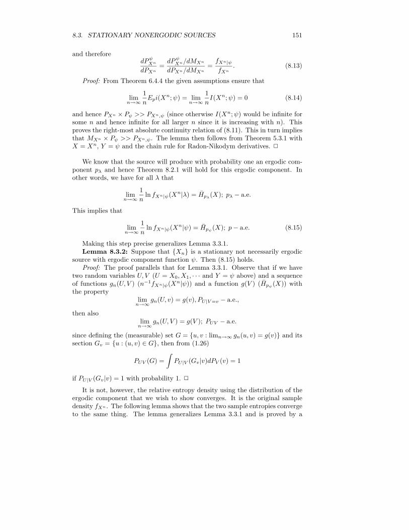
8.3. STATIONARY NONERGODIC SOURCES 151
and thereforedPψ
Xn
dPXn
=dPψ
Xn/dMXn
dPXn/dMXn
=fXn|ψfXn
. (8.13)
Proof: From Theorem 6.4.4 the given assumptions ensure that
limn→∞
1n
Epi(Xn;ψ) = limn→∞
1n
I(Xn;ψ) = 0 (8.14)
and hence PXn × Pψ >> PXn,ψ (since otherwise I(Xn;ψ) would be infinite forsome n and hence infinite for all larger n since it is increasing with n). Thisproves the right-most absolute continuity relation of (8.11). This in turn impliesthat MXn × Pψ >> PXn,ψ. The lemma then follows from Theorem 5.3.1 withX = Xn, Y = ψ and the chain rule for Radon-Nikodym derivatives. 2
We know that the source will produce with probability one an ergodic com-ponent pλ and hence Theorem 8.2.1 will hold for this ergodic component. Inother words, we have for all λ that
limn→∞
1n
ln fXn|ψ(Xn|λ) = Hpλ(X); pλ − a.e.
This implies that
limn→∞
1n
ln fXn|ψ(Xn|ψ) = Hpψ(X); p − a.e. (8.15)
Making this step precise generalizes Lemma 3.3.1.Lemma 8.3.2: Suppose that Xn is a stationary not necessarily ergodic
source with ergodic component function ψ. Then (8.15) holds.Proof: The proof parallels that for Lemma 3.3.1. Observe that if we have
two random variables U, V (U = X0, X1, · · · and Y = ψ above) and a sequenceof functions gn(U, V ) (n−1fXn|ψ(Xn|ψ)) and a function g(V ) (Hpψ
(X)) withthe property
limn→∞
gn(U, v) = g(v), PU |V =v − a.e.,
then alsolim
n→∞gn(U, V ) = g(V ); PUV − a.e.
since defining the (measurable) set G = u, v : limn→∞ gn(u, v) = g(v) and itssection Gv = u : (u, v) ∈ G, then from (1.26)
PUV (G) =∫
PU |V (Gv|v)dPV (v) = 1
if PU |V (Gv|v) = 1 with probability 1. 2
It is not, however, the relative entropy density using the distribution of theergodic component that we wish to show converges. It is the original sampledensity fXn . The following lemma shows that the two sample entropies convergeto the same thing. The lemma generalizes Lemma 3.3.1 and is proved by a
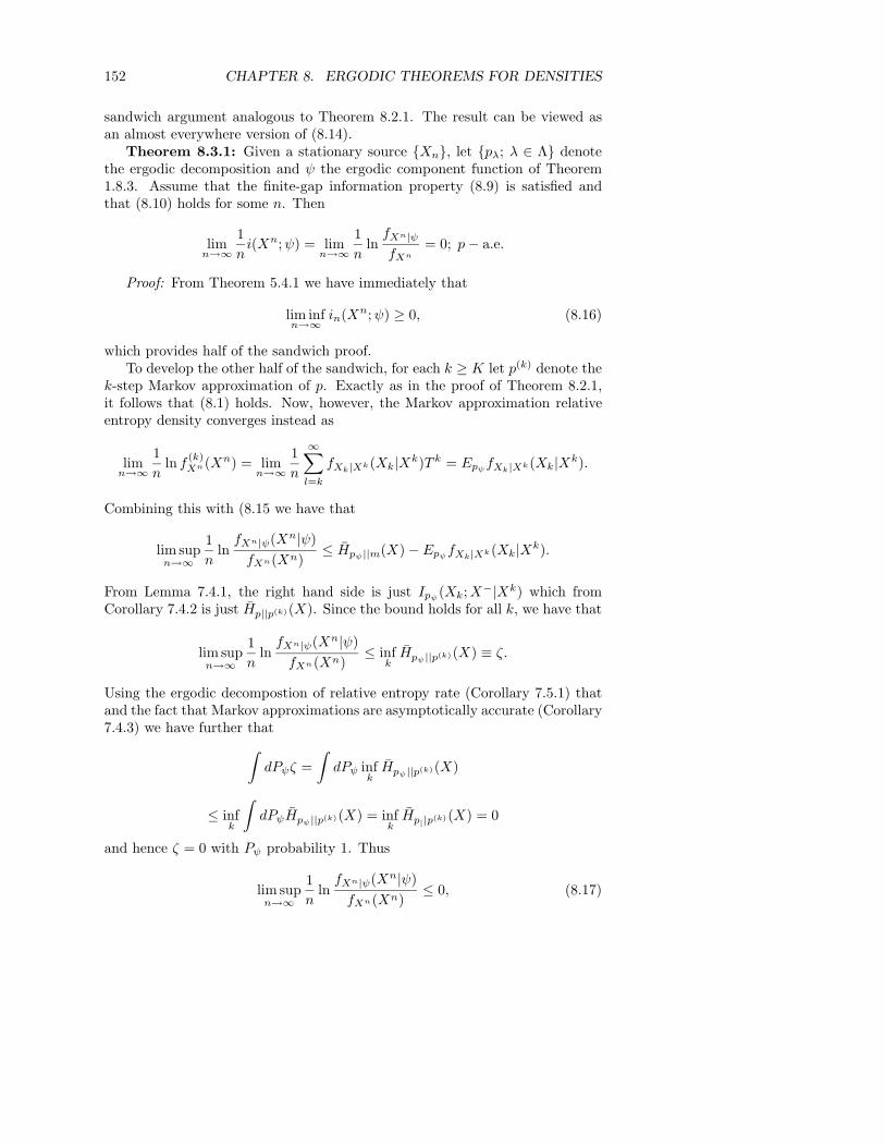
152 CHAPTER 8. ERGODIC THEOREMS FOR DENSITIES
sandwich argument analogous to Theorem 8.2.1. The result can be viewed asan almost everywhere version of (8.14).
Theorem 8.3.1: Given a stationary source Xn, let pλ; λ ∈ Λ denotethe ergodic decomposition and ψ the ergodic component function of Theorem1.8.3. Assume that the finite-gap information property (8.9) is satisfied andthat (8.10) holds for some n. Then
limn→∞
1n
i(Xn;ψ) = limn→∞
1n
lnfXn|ψfXn
= 0; p − a.e.
Proof: From Theorem 5.4.1 we have immediately that
lim infn→∞
in(Xn;ψ) ≥ 0, (8.16)
which provides half of the sandwich proof.To develop the other half of the sandwich, for each k ≥ K let p(k) denote the
k-step Markov approximation of p. Exactly as in the proof of Theorem 8.2.1,it follows that (8.1) holds. Now, however, the Markov approximation relativeentropy density converges instead as
limn→∞
1n
ln f(k)Xn(Xn) = lim
n→∞
1n
∞∑l=k
fXk|Xk(Xk|Xk)T k = EpψfXk|Xk(Xk|Xk).
Combining this with (8.15 we have that
lim supn→∞
1n
lnfXn|ψ(Xn|ψ)
fXn(Xn)≤ Hpψ||m(X) − Epψ
fXk|Xk(Xk|Xk).
From Lemma 7.4.1, the right hand side is just Ipψ(Xk;X−|Xk) which from
Corollary 7.4.2 is just Hp||p(k)(X). Since the bound holds for all k, we have that
lim supn→∞
1n
lnfXn|ψ(Xn|ψ)
fXn(Xn)≤ inf
kHpψ||p(k)(X) ≡ ζ.
Using the ergodic decompostion of relative entropy rate (Corollary 7.5.1) thatand the fact that Markov approximations are asymptotically accurate (Corollary7.4.3) we have further that∫
dPψζ =∫
dPψ infk
Hpψ||p(k)(X)
≤ infk
∫dPψHpψ||p(k)(X) = inf
kHp||p(k)(X) = 0
and hence ζ = 0 with Pψ probability 1. Thus
lim supn→∞
1n
lnfXn|ψ(Xn|ψ)
fXn(Xn)≤ 0, (8.17)
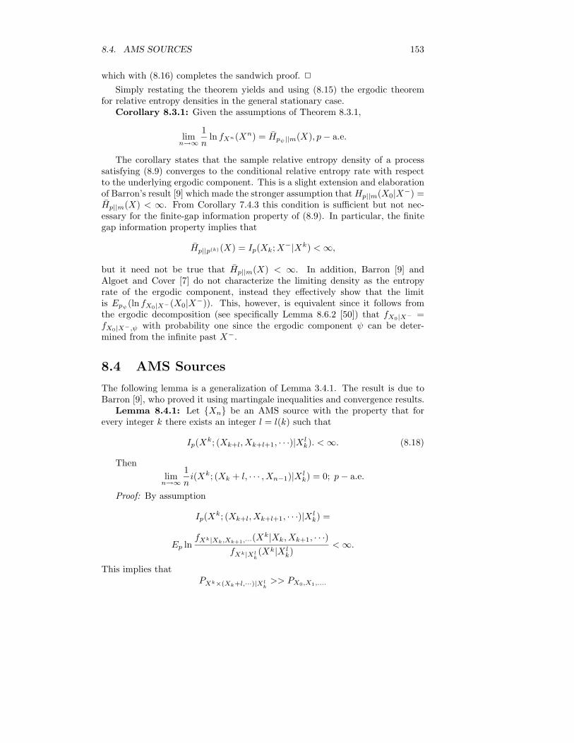
8.4. AMS SOURCES 153
which with (8.16) completes the sandwich proof. 2
Simply restating the theorem yields and using (8.15) the ergodic theoremfor relative entropy densities in the general stationary case.
Corollary 8.3.1: Given the assumptions of Theorem 8.3.1,
limn→∞
1n
ln fXn(Xn) = Hpψ||m(X), p − a.e.
The corollary states that the sample relative entropy density of a processsatisfying (8.9) converges to the conditional relative entropy rate with respectto the underlying ergodic component. This is a slight extension and elaborationof Barron’s result [9] which made the stronger assumption that Hp||m(X0|X−) =Hp||m(X) < ∞. From Corollary 7.4.3 this condition is sufficient but not nec-essary for the finite-gap information property of (8.9). In particular, the finitegap information property implies that
Hp||p(k)(X) = Ip(Xk;X−|Xk) < ∞,
but it need not be true that Hp||m(X) < ∞. In addition, Barron [9] andAlgoet and Cover [7] do not characterize the limiting density as the entropyrate of the ergodic component, instead they effectively show that the limitis Epψ
(ln fX0|X−(X0|X−)). This, however, is equivalent since it follows fromthe ergodic decomposition (see specifically Lemma 8.6.2 [50]) that fX0|X− =fX0|X−,ψ with probability one since the ergodic component ψ can be deter-mined from the infinite past X−.
8.4 AMS Sources
The following lemma is a generalization of Lemma 3.4.1. The result is due toBarron [9], who proved it using martingale inequalities and convergence results.
Lemma 8.4.1: Let Xn be an AMS source with the property that forevery integer k there exists an integer l = l(k) such that
Ip(Xk; (Xk+l, Xk+l+1, · · ·)|X lk). < ∞. (8.18)
Thenlim
n→∞
1n
i(Xk; (Xk + l, · · · , Xn−1)|X lk) = 0; p − a.e.
Proof: By assumption
Ip(Xk; (Xk+l, Xk+l+1, · · ·)|X lk) =
Ep lnfXk|Xk,Xk+1,···(Xk|Xk, Xk+1, · · ·)
fXk|Xlk(Xk|X l
k)< ∞.
This implies thatPXk×(Xk+l,···)|Xl
k>> PX0,X1,....
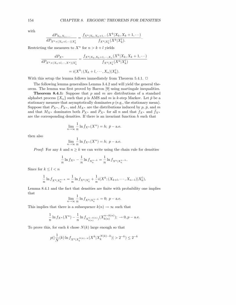
154 CHAPTER 8. ERGODIC THEOREMS FOR DENSITIES
withdPX0,X1,....
dPXk×(Xk+l,···)|Xlk
=fXk|Xk,Xk+1,···(Xk|Xk, Xk + 1, · · ·)
fXk|Xlk(Xk|X l
k)..
Restricting the measures to Xn for n > k + l yields
dPXn
dPXk×(Xk+l,···,Xn)|Xlk
=fXk|Xk,Xk+1,···,Xn
(Xk|Xk, Xk + 1, · · ·)fXk|Xl
k(Xk|X l
k)
= i(Xk; (Xk + l, · · · , Xn)|X lk).
With this setup the lemma follows immediately from Theorem 5.4.1. 2
The following lemma generalizes Lemma 3.4.2 and will yield the general the-orem. The lemma was first proved by Barron [9] using martingale inequalities.
Theorem 8.4.1: Suppose that p and m are distributions of a standardalphabet process Xn such that p is AMS and m is k-step Markov. Let p be astationary measure that asymptotically dominates p (e.g., the stationary mean).Suppose that PXn , PXn , and MXn are the distributions induced by p, p, and mand that MXn dominates both PXn and PXn for all n and that fXn and fXn
are the corresponding densities. If there is an invariant function h such that
limn→∞
1n
ln fXn(Xn) = h; p − a.e.
then alsolim
n→∞
1n
ln fXn(Xn) = h; p − a.e.
Proof: For any k and n ≥ k we can write using the chain rule for densities
1n
ln fXn − 1n
ln fXn−kk
=1n
ln fXk|Xn−kk
.
Since for k ≤ l < n
1n
ln fXk|Xn−kk
=1n
ln fXk|Xlk
+1n
i(Xk; (Xk+l, · · · , Xn−1)|X lk),
Lemma 8.4.1 and the fact that densities are finite with probability one impliesthat
limn→∞
1n
ln fXk|Xn−kk
= 0; p − a.e.
This implies that there is a subsequence k(n) → ∞ such that
1n
ln fXn(Xn) − 1n
ln fX
n−k(n)k(n) )
(Xn−k(n)k(n) ); → 0, p − a.e.
To prove this, for each k chose N(k) large enough so that
p(| 1N
(k) ln fXk|XN(k)−k
k
(Xk|XN(k)−kk )| > 2−k) ≤ 2−k
8.4. AMS SOURCES 155
and then let k(n) = k for N(k) ≤ n < N(k + 1). Then from the Borel-Cantellilemma we have for any ε that
p(| 1N(k)
ln fXk|XN(k)−k
k
(Xk|XN(k)−kk )| > ε i.o.) = 0
and hence
limn→∞
1n
ln fXn(Xn) = limn→∞
1n
ln fX
n−k(n)k(n)
(Xn−k(n)k(n) ); p − a.e.
In a similar manner we can also choose the sequence so that
limn→∞
1n
ln fXn(Xn) = limn→∞
1n
ln fX
n−k(n)k(n)
(Xn−k(n)k(n) ); p − a.e.
From Markov’s inequality
p(1n
ln fXn−kk
(Xn−kk ) ≥ 1
nln fXn−k
k(Xn−k
k ) + ε)
= p(fXn−k
k(Xn−k
k )
fXn−kk
(Xn−kk )
≥ enε) ≤ e−nε
∫dp
fXn−kk
(Xn−kk )
fXn−kk
(Xn−kk )
= e−nε
∫dmfXn−k
k(Xn−k
k ) = e−nε.
Hence again invoking the Borel-Cantelli lemma we have that
p(1n
ln fXn−kk
(Xn−kk ) ≥ 1
nln fXn−k
k(Xn−k
k ) + ε i.o.) = 0
and therefore
lim supn→∞
1n
ln fXn−kk
(Xn−kk ) ≤ h, p − a.e. (8.19)
The above event is in the tail σ-field⋂
n σ(Xn, Xn+1, · · ·) since h is invariantand p dominates p on the tail σ-field. Thus
lim supn→∞
1n
ln fX
n−k(n)k(n)
(Xn−k(n)k(n) ) ≤ h; p − a.e.
and hence
lim supn→∞
1n
ln fXn(Xn) ≤ h; p − a.e.
which half proves the lemma.Since p asymptotically dominates p, given ε > 0 there is a k such that
p( limn→∞
n−1f(Xn−kk ) = h) ≥ 1 − ε.
156 CHAPTER 8. ERGODIC THEOREMS FOR DENSITIES
Again applying Markov’s inequality and the Borel-Cantelli lemma as previouslywe have that
lim infn→∞
1n
lnf
Xn−k(n)k(n)
(Xn−k(n)k(n) )
fX
n−k(n)k(n)
(Xn−k(n)k(n) )
≥ 0; p − a.e.
which implies that
p(lim infn→∞
1n
fX
n−k(n)k(n)
(Xn−kk ) ≥ h) ≥ ε
and hence also thatp(lim inf
n→∞
1n
fXn(Xn) ≥ h) ≥ ε.
Since ε can be made arbitrarily small, this proves that p-a.e. lim inf n−1hn ≥ h,which completes the proof of the lemma. 2
We can now extend the ergodic theorem for relative entropy densities to thegeneral AMS case.
Corollary 8.4.1: Given the assumptions of Theorem 8.4.1,
limn→∞
1n
ln fXn(Xn) = Hpψ(X),
where pψ is the ergodic component of the stationary mean p of p.Proof: The proof follows immediately from Theorem 8.4.1 and Corollary
8.3.1, the ergodic theorem for the relative entropy density for the stationarymean. 2
8.5 Ergodic Theorems for Information Densi-ties.
As an application of the general theorem we prove an ergodic theorem for mutualinformation densities for stationary and ergodic sources. The result can beextended to AMS sources in the same manner that the results of Section 8.3were extended to those of Section 8.4. As the stationary and ergodic resultsuffices for the coding theorems and the AMS conditions are messy, only thestationary case is considered here. The result is due to Barron [9].
Theorem 8.5.1: Let Xn, Yn be a stationary ergodic pair random pro-cess with standard alphabet. Let PXnY n , PXn , and PY n denote the induceddistributions and assume that for all n PXn × PY n >> PXnY n and hence theinformation densities
in(Xn;Y n) =dPXnY n
d(PXn × PY n)
are well defined. Assume in addition that both the Xn and Yn processeshave the finite-gap information property of (8.9) and hence by the comment
8.5. ERGODIC THEOREMS FOR INFORMATION DENSITIES. 157
following Corollary 7.3.1 there is a K such that both processes satisfy the K-gap property
I(XK ;X−|XK) < ∞, I(YK ;Y −|Y K) < ∞.
Thenlim
n→∞
1n
in(Xn;Y n) = I(X;Y ); p − a.e..
Proof: Let Zn = (Xn, Yn). Let MXn = P(K)Xn and MY n = P
(K)Y n denote
the Kth order Markov approximations of Xn and Yn, respectively. Thefinite-gap approximation implies as in Section 8.3 that the densities
fXn =dPXn
dMXn
andfY n =
dPY n
dMY n
are well defined. From Theorem 8.2.1
limn→∞
1n
ln fXn(Xn) = HpX ||p(K)
X
(X0|X−) = I(Xk;X−|Xk) < ∞,
limn→∞
1n
ln fY n(Y n) = I(Yk;Y −|Y k) < ∞.
Define the measures MZn by MXn × MY n . Then this is a K-step Markovsource and since
MXn × MY n >> PXn × PY n
>> PXn,Y n = PZn ,
the density
fZn =dPZn
dMZn
is well defined and from Theorem 8.2.1 has a limit
limn→∞
1n
ln fZn(Zn) = Hp||m(Z0|Z−).
If the density in(Xn, Y n) is infinite for any n, then it is infinite for all largern and convergence is trivially to the infinite information rate. If it is finite, thechain rule for densities yields
1n
in(Xn;Y n) =1n
ln fZn(Zn) − 1n
ln fXn(Xn) − 1n
ln fY n(Y n)
→n→∞
Hp||p(k)(Z0|Z−) − Hp||p(k)(X0|X−) − Hp||p(k)(Y0|Y −)
= Hp||p(k)(X,Y ) − Hp||p(k)(X) − Hp||p(k)(Y ).
The limit is not indeterminate ( of the form ∞−∞) because the two subtractedterms are finite. Since convergence is to a constant, the constant must also bethe limit of the expected values of n−1in(Xn, Y n), that is, I(X;Y ). 2

158 CHAPTER 8. ERGODIC THEOREMS FOR DENSITIES
Chapter 9
Channels and Codes
9.1 Introduction
We have considered a random process or source Xn as a sequence of randomentities, where the object produced at each time could be quite general, e.g.,a random variable, vector, or waveform. Hence sequences of pairs of randomobjects such as Xn, Yn are included in the general framework. We now focuson the possible interrelations between the two components of such a pair process.In particular, we consider the situation where we begin with one source, sayXn, called the input and use either a random or a deterministic mapping toform a new source Yn, called the output. We generally refer to the mappingas a channel if it is random and a code if it is deterministic. Hence a code isa special case of a channel and results for channels will immediately imply thecorresponding results for codes. The initial point of interest will be conditionson the structure of the channel under which the resulting pair process Xn, Ynwill inherit stationarity and ergodic properties from the original source Xn.We will also be interested in the behavior resulting when the output of onechannel serves as the input to another, that is, when we form a new channelas a cascade of other channels. Such cascades yield models of a communicationsystem which typically has a code mapping (called the encoder) followed by achannel followed by another code mapping (called the decoder).
A fundamental nuisance in the development is the notion of time. So far wehave considered pair processes where at each unit of time, one random object isproduced for each coordinate of the pair. In the channel or code example, thiscorresponds to one output for every input. Interesting communication systemsdo not always easily fit into this framework, and this can cause serious problemsin notation and in the interpretation and development of results. For example,suppose that an input source consists of a sequence of real numbers and letT denote the time shift on the real sequence space. Suppose that the outputsource consists of a binary sequence and let S denote its shift. Suppose alsothat the channel is such that for each real number in, three binary symbols are
159
160 CHAPTER 9. CHANNELS AND CODES
produced. This fits our usual framework if we consider each output variable toconsist of a binary three-tuple since then there is one output vector for eachinput symbol. One must be careful, however, when considering the stationarityof such a system. Do we consider the output process to be physically stationaryif it is stationary with respect to S or with respect to S3? The former mightmake more sense if we are looking at the output alone, the latter if we are lookingat the output in relation to the input. How do we define stationarity for the pairprocess? Given two sequence spaces, we might first construct a shift on the pairsequence space as simply the cartesian product of the shifts, e.g., given an inputsequence x and an output sequence y define a shift T ∗ by T ∗(x, y) = (Tx, Sy).While this might seem natural given simply the pair random process Xn, Yn,it is not natural in the physical context that one symbol of X yields threesymbols of Y . In other words, the two shifts do not correspond to the sameamount of time. Here the more physically meaningful shift on the pair spacewould be T ′(x, y) = (Tx, S3y) and the more physically meaningful questions onstationarity and ergodicity relate to T ′ and not to T ∗. The problem becomeseven more complicated when channels or codes produce a varying number ofoutput symbols for each input symbol, where the number of symbols dependson the input sequence. Such variable rate codes arise often in practice, especiallyfor noiseless coding applications such as Huffman, Lempel-Ziv, and arithmeticcodes. (See [140] for a survey of noiseless coding.) While we will not treat suchvariable rate systems in any detail, they point out the difficulty that can ariseassociating the mathematical shift operation with physical time when we areconsidering cartesian products of spaces, each having their own shift.
There is no easy way to solve this problem notationally. We adopt thefollowing view as a compromise which is usually adequate for fixed-rate systems.We will be most interested in pair processes that are stationary in the physicalsense, that is, whose statistics are not changed when both are shifted by anequal amount of physical time. This is the same as stationarity with respectto the product shift if the two shifts correspond to equal amounts of physicaltime. Hence for simplicity we will usually focus on this case. More general caseswill be introduced when appropriate to point out their form and how they canbe put into the matching shift structure by considering groups of symbols anddifferent shifts. This will necessitate occasional discussions about what is meantby stationarity or ergodicity for a particular system.
The mathematical generalization of Shannon’s original notions of sources,codes, and channels are due to Khinchine [72] [73]. Khinchine’s results char-acterizing stationarity and ergodicity of channels were corrected and developedby Adler [2].
9.2 Channels
Say we are given a source [A,X, µ], that is, a sequence of A-valued randomvariables Xn;n ∈ T defined on a common probability space (Ω,F , P ) havinga process distribution µ defined on the measurable sequence space (BT ,BA
T ).
9.2. CHANNELS 161
We shall let X = Xn;n ∈ T denote the sequence-valued random variable,that is, the random variable taking values in AT according to the distributionµ. Let B be another alphabet with a corresponding measurable sequence space(AT ,BB
T ). We assume as usual that A and B are standard and hence soare their sequence spaces and cartesian products. A channel [A, ν,B] withinput alphabet A and output alphabet B (we denote the channel simply by νwhen these alphabets are clear from context) is a family of probability measuresνx;x ∈ AT on (BT ,BB
T ) (the output sequence space) such that for everyoutput event F ∈ BB
T νx(F ) is a measurable function of x. This measurabilityrequirement ensures that the set function p specified on the joint input/outputspace (AT × BT ), BA
T × BBT ) by its values on rectangles as
p(G × F ) =∫
G
dµ(x)νx(F );F ∈ BBT , G ∈ BA
T ,
is well defined. The set function p is nonnegative, normalized, and countablyadditive on the field generated by the rectangles G × F , G ∈ BA
T , F ∈ BBT .
Thus p extends to a probability measure on the joint input/output space, whichis sometimes called the hookup of the source µ and channel ν. We will often de-note this joint measure by µν. The corresponding sequences of random variablesare called the input/output process.
Thus a channel is a probability measure on the output sequence space foreach input sequence such that a joint input/output probability measure is well-defined. The above equation shows that a channel is simply a regular conditionalprobability, in particular,
νx(F ) = p((x, y) : y ∈ F |x);F ∈ BBT , x ∈ AT .
We can relate a channel to the notation used previously for conditionaldistributions by using the sequence-valued random variables X = Xn;n ∈ T and Y = Yn;n ∈ T :
νx(F ) = PY |X(F |x). (9.1)
Eq. (1.26) then provides the probability of an arbitrary input/output event:
p(F ) =∫
dµ(x)νx(Fx),
where Fx = y : (x, y) ∈ F is the section of F at x.If we start with a hookup p, then we can obtain the input distribution µ as
µ(F ) = p(F × BT );F ∈ BAT .
Similarly we can obtain the output distribution, say η, via
η(F ) = p(AT × F );F ∈ BBT .
Suppose one now starts with a pair process distribution p and hence alsowith the induced source distribution µ. Does there exist a channel ν for which
162 CHAPTER 9. CHANNELS AND CODES
p = µν? The answer is yes since the spaces are standard. One can always definethe conditional probability νx(F ) = P (F ×AT |X = x) for all input sequences x,but this need not possess a regular version, that is, be a probability measure forall x, in the case of arbitrary alphabets. If the alphabets are standard, however,we have seen that a regular conditional probability measure always exists.
9.3 Stationarity Properties of Channels
We now define a variety of stationarity properties for channels that are relatedto, but not the same as, those for sources. The motivation behind the var-ious definitions is that stationarity properties of channels coupled with thoseof sources should imply stationarity properties for the resulting source-channelhookups.
The classical definition of a stationary channel is the following: Suppose thatwe have a channel [A, ν,B] and suppose that TA and TB are the shifts on theinput sequence space and output sequence space, respectively. The channel isstationary with respect to TA and TB or (TA, TB)-stationary if
νx(T−1B F ) = νTAx(F ), x ∈ AT , F ∈ BB
T . (9.2)
If the transformations are clear from context then we simply say that the chan-nel is stationary. Intuitively, a right shift of an output event yields the sameprobability as the left shift of an input event. The different shifts are requiredbecause in general only TAx and not T−1
A x exists since the shift may not beinvertible and in general only T−1
B F and not TBF exists for the same reason. Ifthe shifts are invertible, e.g., the processes are two-sided, then the definition isequivalent to
νTAx(TBF ) = νT−1A
x(T−1B F ) = νx(F ), all x ∈ AT , F ∈ BB
T (9.3)
that is, shifting the input sequence and output event in the same direction doesnot change the probability.
The fundamental importance of the stationarity of a channel is contained inthe following lemma.
Lemma 9.3.1: If a source [A,µ], stationary with respect to TA, is connectedto channel [A, ν,B], stationary with respect to TA and TB , then the resultinghookup µν is also stationary (with respect to the cartesian product shift T =TA×B = TA × TB defined by T (x, y) = (TAx, TBy)).
Proof: We have that
µν(T−1F ) =∫
dµ(x)νx((T−1F )x).
Now(T−1F )x = y : T (x, y) ∈ F = y : (TAx, TBy) ∈ F
= y : TBy ∈ FTAx = T−1B FTAx (9.4)
9.3. STATIONARITY PROPERTIES OF CHANNELS 163
and henceµν(T−1F ) =
∫dµ(x)νx(T−1
B FTAx).
Since the channel is stationary, however, this becomes
µν(T−1F ) =∫
dµ(x)νTAx(FTAx) =∫
dµT−1A (x)νx(Fx),
where we have used the change of variables formula. Since µ is stationary,however, the right hand side is ∫
dµ(x)νx(F ),
which proves the lemma. 2
Suppose next that we are told that a hookup µν is stationary. Does it thenfollow that the source µ and channel ν are necessarily stationary? The sourcemust be since
µ(T−1A F ) = µν((TA × TB)−1(F × BT )) = µν(F × BT ) = µ(F ).
The channel need not be stationary, however, since, for example, the stationaritycould be violated on a set of µ measure 0 without affecting the proof of theabove lemma. This suggests a somewhat weaker notion of stationarity which ismore directly related to the stationarity of the hookup. We say that a channel[A, ν,B] is stationary with respect to a source [A,µ] if µν is stationary. We alsostate that a channel is stationary µ-a.e. if it satisfies (9.2) for all x in a set ofµ-probability one. If a channel is stationary µ-a.e. and µ is stationary, thenthe channel is also stationary with respect to µ. Clearly a stationary channelis stationary with respect to all stationary sources. The reason for this moregeneral view is that we wish to extend the definition of stationary channels toasymptotically mean stationary channels. The general definition extends; theclassical definition of stationary channels does not.
Observe that the various definitions of stationarity of channels immediatelyextend to block shifts since they hold for any shifts defined on the input andoutput sequence spaces, e.g., a channel stationary with respect to TN
A and TKB
could be a reasonable model for a channel or code that puts out K symbolsfrom an alphabet B every time it takes in N symbols from an alphabet A. Weshorten the name (TN
A , TKB )-stationary to (N,K)-stationary channel in this case.
A stationary channel (without modifiers) is simply a (1,1)-stationary channel inthis sense.
The most general notion of stationarity that we are interested in is that ofasymptotic mean stationarity We define a channel [A, ν,B] to be asymptoticallymean stationary or AMS for a source [A,µ] with respect to TA and TB if thehookup µν is AMS with respect to the product shift TA × TB . As in the sta-tionary case, an immediate necessary condition is that the input source be AMSwith respect to TA. A channel will be said to be (TA, TB)-AMS if the hookupis (TA, TB)-AMS for all TA-AMS sources.
164 CHAPTER 9. CHANNELS AND CODES
The following lemma shows that an AMS channel is indeed a generalizationof the idea of a stationary channel and that the stationary mean of a hookup ofan AMS source to a stationary channel is simply the hookup of the stationarymean of the source to the channel.
Lemma 9.3.2: Suppose that ν is (TA, TB)-stationary and that µ is AMSwith respect to TA. Let µ denote the stationary mean of µ and observe that µνis stationary. Then the hookup µν is AMS with stationary mean
µν = µν.
Thus, in particular, ν is an AMS channel.Proof: We have that
(T−iF )x = y : (x, y) ∈ T−iF = y : T i(x, y) ∈ F
= y : (T iAx, T i
By) ∈ F = y : T iBy ∈ FT i
Ax = T−i
B FT iA
x (9.5)
and therefore since ν is stationary
µν(T−iF ) =∫
dµ(x)νx(T−iB FT i
Ax)
=∫
dµ(x)νT iA
x(FT iA
x) =∫
dµT−iA (x)νx(F ).
Therefore1n
n−1∑i=0
µν(T−iF )
=1n
n−1∑i=0
∫dµT−i
A (x)νx(F ) →n→∞
∫dµ(x)νx(F ) = µν(F )
from Lemma 6.5.1 of [50]. This proves that µν is AMS and that the stationarymean is µν. 2
A final property crucial to quantifying the behavior of random processes isthat of ergodicity. Hence we define a (stationary, AMS) channel ν to be ergodicwith respect to (TA, TB) if it has the property that whenever a (stationary, AMS)ergodic source (with respect to TA) is connected to the channel, the overallinput/output process is (stationary, AMS) ergodic. The following modificationof Lemma 6.7.4 of [50] is the principal tool for proving a channel to be ergodic.
Lemma 9.3.3: An AMS (stationary) channel [A, ν,B] is ergodic if for allAMS (stationary) sources µ and all sets of the form F = FA×FB, G = GA×GB
for rectangles FA, GA ∈ B∞A and FB, GB ∈ B∞
B we have that for p = µν
limn→∞
1n
n−1∑i=0
p(T−iA×BF
⋂G) = p(F )p(G), (9.6)
where p is the stationary mean of p (p if p is already stationary).
9.4. EXAMPLES OF CHANNELS 165
Proof: The proof parallels that of Lemma 6.7.4 of [50]. The result doesnot follow immediately from that lemma since the collection of given sets doesnot itself form a field. Arbitrary events F,G ∈ B∞
A×B can be approximatedarbitrarily closely by events in the field generated by the above rectangles andhence given ε > 0 we can find finite disjoint rectangles of the given form Fi,Gi, i = 1, · · · , L such that if F0 =
⋃Li=1 Fi and G0 =
⋃Li=1 Gi, then p(F∆F0),
p(G∆G0), p(F∆F0), and p(G∆G0) are all less than ε. Then
| 1n
n−1∑k=0
p(T−kF⋂
G) − p(F )p(G)|
≤ | 1n
n−1∑k=0
p(T−kF⋂
G) − 1n
n−1∑k=0
p(T−kF0
⋂G0)|
+| 1n
n−1∑k=0
p(T−kF0
⋂G0) − p(F0)p(G0)| + |p(F0)p(G0) − p(F )p(G)|.
Exactly as in Lemma 6.7.4 of [50], the rightmost term is bound above by 2εand the first term on the left goes to zero as n → ∞. The middle term is theabsolute magnitude of
1n
n−1∑k=0
p(T−k⋃i
Fi
⋂ ⋃j
Gj) − p(⋃i
Fi)p(⋃j
Gj)
=∑i,j
(1n
n−1∑k=0
p(T−kFi
⋂Gj) − p(Fi)p(Gj)
).
Each term in the finite sum converges to 0 by assumption. Thus p is ergodicfrom Lemma 6.7.4 of [50]. 2
Because of the specific class of sets chosen, the above lemma consideredseparate sets for shifting and remaining fixed, unlike using the same set forboth purposes as in Lemma 6.7.4 of [50]. This was required so that the crossproducts in the final sum considered would converge accordingly.
9.4 Examples of Channels
In this section a variety of examples of channels are introduced, ranging from thetrivially simple to the very complicated. The first two channels are the simplest,the first being perfect and the second being useless (at least for communicationpurposes).
166 CHAPTER 9. CHANNELS AND CODES
Example 9.4.1: Noiseless Channel
A channel [A, ν,B] is said to be noiseless if A = B and
νx(F ) =
1 x ∈ F0 x 6∈ F
that is, with probability one the channel puts out what goes in. Such a channelis clearly stationary and ergodic.
Example 9.4.2: Completely Random Channel
Suppose that η is a probability measure on the output space (BT ,BBT ) and
define a channelνx(F ) = η(F ), F ∈ BB
T , x ∈ AT .
Then it is easy to see that the input/output measure satisfies
p(G × F ) = η(F )µ(G);F ∈ BBT , G ∈ BA
T ,
and hence the input/output measure is a product measure and the input andoutput sequences are therefore independent of each other. This channel is calleda completely random channel or product channel because the output is indepen-dent of the input. This channel is quite useless because the output tells usnothing of the input. The completely random channel is stationary (AMS) ifthe measure η is stationary (AMS). Perhaps surprisingly, such a channel neednot be ergodic even if η is ergodic since the product of two stationary and er-godic sources need not be ergodic. (See, e.g., [21].) We shall later see that if ηis also assumed to be weakly mixing, then the resulting channel is ergodic.
A generalization of the noiseless channel that is of much greater interest isthe deterministic channel. Here the channel is not random, but the output isformed by a general mapping of the input rather than being the input itself.
Example 9.4.3: Deterministic Channel and Sequence Coders
A channel [A, ν,B] is said to be deterministic or nonrandom if each input stringis mapped into a fixed output string, that is, if there is a mapping f : AT → BT
such that
νx(G) =
1 f(x) ∈ G0 f(x) 6∈ G
.
The mapping f must be measurable in order to satisfy the measurability as-sumption of the channel. Note that such a channel can also be written as
νx(G) = 1f−1(G)(x).
9.4. EXAMPLES OF CHANNELS 167
Define a sequence coder as a deterministic channel, that is, a measurablemapping from one sequence space into another. It is easy to see that for adeterministic code we have a hookup specified by
p(F × G) = µ(F⋂
f−1(G))
and an output process with distribution
η(G) = µ(f−1(G)).
A sequence coder is said to be (TA, TB)-stationary (or just stationary) or(TN
A , TKB )-stationary (or just (N,K)-stationary) if the corresponding channel
is. Thus a sequence coder f is stationary if and only if f(TAx) = TBf(x) andit is (N,K)- stationary if and only if f(TN
A x) = TKB f(x).
Lemma 9.4.1: A stationary deterministic channel is ergodic.Proof: From Lemma 9.3.3 it suffices to show that
limn→∞
1n
n−1∑i=0
p(T−iA×BF
⋂G) = p(F )P (G)
for all rectangles of the form F = FA × FB , FA ∈ BBT , FB ∈ BA
T andG = GA × GB . Then
p(T−iA×BF
⋂G) = p((T−i
A FA
⋂GA) × (T−i
B FB
⋂GB))
= µ((T−iA FA
⋂GA)
⋂f−1(T−i
B FB
⋂GB)).
Since f is stationary and since inverse images preserve set theoretic operations,
f−1(T−iB FB
⋂GB) = T−i
A f−1(FB)⋂
f−1(GB)
and hence1n
n−1∑i=0
p(T−iA×BF
⋂G)
=1n
n−1∑i=0
µ(T−iA (FA
⋂f−1(FB))
⋂GA
⋂f−1(GB))
→n→∞
µ(FA
⋂f−1(FB))µ(GA
⋂f−1(GB)) = p(FA × FB)p(GA × GB)
since µ is ergodic. This means that the rectangles meet the required condition.Some algebra then will show that finite unions of disjoint sets meeting theconditions also meet the conditions and that complements of sets meeting theconditions also meet them. This implies from the good sets principle (see, forexample, p. 14 of [50]) that the field generated by the rectangles also meets thecondition and hence the lemma is proved. 2
168 CHAPTER 9. CHANNELS AND CODES
A stationary sequence coder has a simple and useful structure. Suppose onehas a mapping f : AT → B, that is, a mapping that maps an input sequence intoan output letter. We can define a complete output sequence y corresponding toan input sequence x by
yi = f(T iAx); i ∈ T , (9.7)
that is, we produce an output, then shift or slide the input sequence by one timeunit, and then we produce another output using the same function, and so on. Amapping of this form is called an infinite length sliding block code because it pro-duces outputs by successively sliding an infinite length input sequence and eachtime using a fixed mapping to produce the output. The sequence-to-letter map-ping implies a sequence coder, say f , defined by f(x) = f(T i
Ax); i ∈ T . Fur-thermore, f(TAx) = TB f(x), that is, a sliding block code induces a stationarysequence coder. Conversely, any stationary sequence coder f induces a slidingblock code f for which (9.7) holds by the simple identification f(x) = (f(x))0,the output at time 0 of the sequence coder. Thus the ideas of stationary se-quence coders mapping sequences into sequences and sliding block codes map-ping sequences into letters by sliding the input sequence are equivalent. We cansimilarly define an (N,K)-sliding block code which is a mapping f : AT → BK
which forms an output sequence y from an input sequence x via the construction
yKiK = f(TNi
A x).
By a similar argument, (N,K)-sliding block coders are equivalent to (N,K)-stationary sequence coders. When dealing with sliding block codes we willusually assume for simplicity that K is 1. This involves no loss in generalitysince it can be made true by redefining the output alphabet.
Example 9.4.4: B-processes
The above construction using sliding block or stationary codes provides an easydescription of an important class of random processes that has several niceproperties. A process is said to be a B-process or Bernoulli process if it can bedefined as a stationary coding of an independent identically distributed (i.i.d.)process. Let µ denote the original distribution of the i.i.d. process and let ηdenote the induced output distribution. Then for any output events F and G
η(F⋂
T−nB G) = µ(f−1(F
⋂T−n
B G)) = µ(f−1(F )⋂
T−nA f−1(G)),
since f is stationary. But µ is stationary and mixing since it is i.i.d. (see Section6.7 of [50]) and hence this probability converges to
µ(f−1(F ))µ(f−1(G)) = η(F )η(G)
and hence η is also mixing. Thus a B-process is mixing of all orders and henceis ergodic with respect to T n
B for all positive integers n.While codes that depend on infinite input sequences may not at first glance
seem to be a reasonable physical model of a coding system, it is possible for
9.4. EXAMPLES OF CHANNELS 169
such codes to depend on the infinite sequence only through a finite number ofcoordinates. In addition, some real codes may indeed depend on an unboundedlylarge number of past inputs because of feedback.
Suppose that we consider two-sided processes and that we have a measurablemapping
φ :D×
i=−MAi → B
and we define a sliding block code by
f(x) = φ(xi−M , · · · , x0, · · · , xi+D),
then f is a stationary sequence coder. The mapping φ is also called a slidingblock code or a finite-length sliding block code or a finite-window sliding blockcode. M is called the memory of the code and D is called the delay of the codesince M past source symbols and D future symbols are required to produce thecurrent output symbol. The window length or constraint length of the code isM +D+1, the number of input symbols viewed to produce an output symbol. IfD = 0 the code is said to be causal. If M = 0 the code is said to be memoryless.
There is a problem with the above model if we wish to code a one-sidedsource since if we wish to start coding at time 0, there are no input symbols withnegative indices. Hence we either must require the code be memoryless (M = 0)or we must redefine the code for the first M instances (e.g., by “stuffing” thecode register with arbitrary symbols) or we must only define the output for timesi ≥ M . For two-sided sources a finite-length sliding block code is stationary.In the one-sided case it is not even defined precisely unless it is memoryless, inwhich case it is stationary.
Another case of particular interest is when we have a measurable mappingγ : AN → BK and we define a sequence coder f(x) = y by
yKnK = (ynK , ynK+1, · · · , y(n+1)K−1) = γ(xN
nN ),
that is, the input is parsed into nonoverlapping blocks of length N and each issuccessively coded into a block of length K outputs without regard to past orprevious input or output blocks. Clearly N input time units must correspondto K output time units in physical time if the code is to make sense. A code ofthis form is called a block code and it is a special case of an (N,K) sliding blockcode. Such a code is trivially (TN
A , TKA )-stationary.
We now return to genuinely random channels. The next example is perhapsthe most popular model for a noisy channel because of its simplicity.
Example 9.4.5: Memoryless channels
Suppose that qx0(·) is a probability measure on BB for all x0 ∈ A and that forfixed F ,qx0(F ) is a measurable function of x0. Let ν be a channel specified byits values on output rectangles by
νx( ×i∈J
Fi) =∏i∈J
qxi(Fi),
170 CHAPTER 9. CHANNELS AND CODES
for any finite index set J ⊂ T . Then ν is said to be a memoryless channel.Intuitively,
Pr(Yi ∈ Fi; i ∈ J |X) =∏i∈J
Pr(Yi ∈ Fi|Xi).
For later use we pause to develop a useful inequality for mutual informationbetween the input and output of a memoryless channel. For contrast we alsodescribe the corresponding result for a memoryless source and an arbitrarychannel.
Lemma 9.4.2: Let Xn be a source with distribution µ and let ν be achannel. Let Xn, Yn be the hookup with distribution p. If the channel ismemoryless, then for any n
I(Xn;Y n) ≤n−1∑i=0
I(Xi;Yi)
If instead the source is memoryless, then the inequality is reversed:
I(Xn;Y n) ≥n−1∑i=0
I(Xi;Yi).
Thus if both source and channel are memoryless,
I(Xn;Y n) =n−1∑i=0
I(Xi;Yi).
Proof: First suppose that the process is discrete. Then
I(Xn;Y n) = H(Y n) − H(Y n|Xn).
Since by construction
PY n|Xn(yn|xn) =n−1∏i=0
PY0|X0(yi|xi)
an easy computation shows that
H(Y n|Xn) =n−1∑i=0
H(Yi|Xi).
This combined with the inequality
H(Y n) ≤n−1∑i=0
H(Yi)
(Lemma 2.3.2 used several times) completes the proof of the memoryless channelresult for finite alphabets. If instead the source is memoryless, we have
I(Xn;Y n) = H(Xn) − H(Xn|Y n)
9.4. EXAMPLES OF CHANNELS 171
=n−1∑i=0
H(Xi) − H(Xn|Y n).
Extending Lemma 2.3.2 to conditional entropy yields
H(Xn|Y n) ≤n−1∑i=0
H(Xi|Y n)
which can be further overbounded by using Lemma 2.5.2 (the fact that reducingconditioning increases conditional entropy) as
H(Xn|Y n) ≤n−1∑i=0
H(Xi|Yi)
which implies that
I(Xn;Y n) ≥n−1∑i=0
H(Xi) − H(Xi|Yi) =n−1∑i=0
I(Xi;Yi),
which completes the proof for finite alphabets.To extend the result to standard alphabets, first consider the case where the
Y n are quantized to a finite alphabet. If the Yk are conditionally independentgiven Xk, then the same is true for q(Yk), k = 0, 1, · · · , n−1. Lemma 5.5.6 thenimplies that as in the discrete case, I(Xn;Y n) = H(Y n) − H(Y n|Xn) and theremainder of the proof follows as in the discrete case. Letting the quantizersbecome asymptotically accurate then completes the proof. 2
In fact two forms of memorylessness are evident in a memoryless channel.The channel is input memoryless in that the probability of an output eventinvolving Yi; i ∈ k, k + 1, · · · ,m does not involve any inputs before time k,that is, the past inputs. The channel is also input nonanticipatory since thisevent does not depend on inputs after time m, that is, the future inputs. Thechannel is also output memoryless in the sense that for any given input x, outputevents involving nonoverlapping times are independent, i.e.,
νx(Y1 ∈ F1
⋂Y2 ∈ F2) = νx(Y1 ∈ F1)νx(Y2 ∈ F2).
We pin down these ideas in the following examples.
Example 9.4.6: Channels with finite input memory andanticipation
A channel ν is said to have finite input memory of order M if for all one-sidedevents F and all n
νx((Yn, Yn+1, · · ·) ∈ F ) = νx′((Yn, Yn+1, · · ·) ∈ F )
172 CHAPTER 9. CHANNELS AND CODES
whenever xi = x′i for i ≥ n − M . In other words, for an event involving Yi’s
after some time n, knowing only the inputs for the same times and M timeunits earlier completely determines the output probability. Channels with finiteinput memory were introduced by Feinstein [40]. Similarly ν is said to havefinite anticipation of order L if for all one-sided events F and all n
νx((· · · , Yn) ∈ F ) = νx′((· · · , Yn) ∈ F )
provided x′i = xi for i ≤ n+L. That is, at most L future inputs must be known
to determine the probability of an event involving current and past outputs.
Example 9.4.7: Channels with finite output memory
A channel ν is said to have finite output memory of order K if for all one-sidedevents F and G and all inputs x, if k > K then
νx((· · · , Yn) ∈ F⋂
(Yn+k, · · ·) ∈ G) = νx((· · · , Yn) ∈ F )νx((Yn+k, · · ·) ∈ G);
that is, output events involving output samples separated by more than K timeunits are independent. Channels with finite output memory were introduced byWolfowitz [150].
Channels with finite memory and anticipation are historically important asthe first real generalizations of memoryless channels for which coding theoremscould be proved. Furthermore, the assumption of finite anticipation is physi-cally reasonable as a model for real-world communication channels. The finitememory assumptions, however, exclude many important examples, e.g., finite-state or Markov channels and channels with feedback filtering action. Hencewe will emphasize more general notions which can be viewed as approximationsor asymptotic versions of the finite memory assumption. The generalization offinite input memory channels requires some additional tools and is postponedto the next chapter. The notion of finite output memory can be generalized byusing the notion of mixing.
Example 9.4.8: Output mixing channels
A channel is said to be output mixing (or asymptotically output independentor asymptotically output memoryless) if for all output rectangles F and G andall input sequences x
limn→∞
|νx(T−nF⋂
G) − νx(T−nF )νx(G)| = 0.
More generally it is said to be output weakly mixing if
limn→∞
1n
n−1∑i=0
|νx(T−iF⋂
G) − νx(T−iF )νx(G)| = 0.
9.4. EXAMPLES OF CHANNELS 173
Unlike mixing systems, the above definitions for channels place conditions onlyon output rectangles and not on all output events. Output mixing channelswere introduced by Adler [2].
The principal property of output mixing channels is provided by the followinglemma.
Lemma 9.4.3: If a channel is stationary and output weakly mixing, thenit is also ergodic. That is, if ν is stationary and output weakly mixing and if µis stationary and ergodic, then also µν is stationary and ergodic.
Proof: The process µν is stationary by Lemma 9.3.1. To prove that it isergodic it suffices from Lemma 9.3.3 to prove that for all input/output rectanglesof the form F = FB × FA, FB ∈ BA
T , FA ∈ BBT , and G = GB × GA that
limn→∞
1n
n−1∑i=0
µν(T−iF⋂
G) = µν(F )µν(G).
We have that1n
n−1∑i=0
µν(T−iF⋂
G) − m(F )m(G)
=1n
n−1∑i=0
µν((T−iB FB
⋂GB) × (T−i
A FA
⋂GA)) − µν(FB × FA)µν(GB × GA)
=1n
n−1∑i=0
∫T−i
AFA
⋂GA
dµ(x)νx(T−iB FB
⋂GB) − µν(FB × FA)µ(GB × GA)
=
(1n
n−1∑i=0
(∫T−i
AFA
⋂GA
dµ(x)νx(T−iB FB
⋂GB)
−∫
T−iA
FA
⋂GA
dµ(x)νx(T−iB FB)νx(GB)
))+
(1n
n−1∑i=0(∫
T−iA
FA
⋂GA
dµ(x)νx(T−iB FB)νx(GB) − µν(FB × FA)µν(GB × GA)
)).
The first term is bound above by
1n
n−1∑i=0
∫T−i
AFA
⋂GA
dµ(x)|νx(T−iB FB
⋂GB) − νx(T−i
B FB)νx(GB)|
≤∫
dµ(x)1n
n−1∑i=0
|νx(T−iB FB
⋂GB) − νx(T−iFB)νx(GB)|
which goes to zero from the dominated convergence theorem since the integrandconverges to zero from the output weakly mixing assumption. The second term
174 CHAPTER 9. CHANNELS AND CODES
can be expressed using the stationarity of the channel as
∫FA
dµ(x)νx(GB)1n
n−1∑i=0
1FA(T i
Ax)νT iA
x(FB) − µν(F )µν(G).
The ergodic theorem implies that as n → ∞ the sample average goes to itsexpectation ∫
dµ(x)1FA(x)νx(FB) = µν(F )
and hence the above formula converges to 0, proving the lemma. 2
The lemma provides an example of a completely random channel that is alsoergodic in the following corollary.
Corollary 9.4.1: Suppose that ν is a stationary completely random channeldescribed by an output measure η. If η is weakly mixing, then ν is ergodic. Thatis, if µ is stationary and ergodic and η is stationary and weakly mixing, thenµν = µ × η is stationary and ergodic.
Proof: If η is weakly mixing, then the channel ν defined by νx(F ) = η(F ),all x ∈ AT , F ∈ BB
T is output weakly mixing. Thus ergodicity follows fromthe lemma. 2
The idea of a memoryless channel can be extended to a block memorylessor block independent channel, as described next.
Example 9.4.9: Block Memoryless Channels
Suppose now that we have an integers N and K (usually K = N) and a probabil-ity measure qxN (·) on BK
B for each xN ∈ AN such that qxN (F ) is a measurablefunction of xN for each F ∈ BK
B . Let ν be specified by its values on outputrectangles by
νx(y : yi ∈ Gi; i = m, · · · ,m + n − 1) =b n
K c∏i=0
qxNiN
(Gi),
where Gi ∈ BB , all i, where bzc is the largest integer contained in z, and where
Gi =m+(i+1)K−1
×j=m+iK
Fj
with Fj = B if j ≥ m + n. Such channels are called block memoryless channelsor block independent channels. They are a special case of the following class ofchannels.
Example 9.4.10: Conditionally Block Independent Chan-nels
A conditionally block independent or CBI channel resembles the block memory-less channel in that for a given input sequence the outputs are block independent.
9.4. EXAMPLES OF CHANNELS 175
It is more general, however, in that the conditional probabilities of the outputblock may depend on the entire input sequence (or at least on parts of the inputsequence not in the same time block). Thus a channel is CBI if its values onoutput rectangles satisfy
νx(y : yi ∈ Fi; i = m, · · · ,m + n − 1) =b n
K c∏i=0
νx(y : yNiN ∈ Gi).
where as before
Gi =m+(i+1)K−1
×j=m+iK
Fj
with Fj = B if j ≥ m + n. Block memoryless channels are clearly a specialcase of CBI channels. These channels have only finite output memory, butunlike the block memoryless channels they need not have finite input memoryor anticipation.
The primary use of block memoryless channels is in the construction of achannel given finite-dimensional conditional probabilities, that is, one has prob-abilities for output K-tuples given input N -tuples and one wishes to model achannel consistent with these finite-dimensional distributions. The finite dimen-sional distributions themselves may be the result of an optimization problem oran estimate based on observed behavior. An immediate problem is that a chan-nel constructed in this manner may not be stationary, although it is clearly(N,K)-stationary. The next example shows how to modify a block memorylesschannel so as to produce a stationary channel. The basic idea is to occasion-ally insert some random spacing between the blocks so as to “stationarize” thechannel.
Before turning to the example we first develop the technical details requiredfor producing such random spacing.
Random Punctuation Sequences
We demonstrate that we can obtain a sequence with certain properties by sta-tionary coding of an arbitrary stationary and ergodic process. The lemma is avariant of a theorem of Shields and Neuhoff [133] as simplified by Neuhoff andGilbert [108] for sliding block codings of finite alphabet processes. One of theuses to which the result will be put is the same as theirs: constructing slidingblock codes from block codes.
Lemma 9.4.4: Suppose that Xn is a stationary and ergodic process.Then given N and δ > 0 there exists a stationary (or sliding block) codingf : AT → 0, 1, 2 yielding a ternary process Zn with the following properties:
(a) Zn is stationary and ergodic.
(b) Zn has a ternary alphabet 0, 1, 2 and it can output only N -cells of theform 011 · · · 1 (0 followed by N − 1 ones) or individual 2’s. In particular,each 0 is always followed by at exactly N − 1 1’s.
176 CHAPTER 9. CHANNELS AND CODES
(c) For all integers k
1 − δ
N≤ Pr(ZN
k = 011 · · · 1) ≤ 1N
and hence for any n
Pr(Zn is in an N − cell) ≥ 1 − δ.
A process Zn with these properties is called an (N, δ)-random blockingprocess or punctuation sequence Zn.
Proof: A sliding block coding is stationary and hence coding a stationaryand ergodic process will yield a stationary and ergodic process (Lemma 9.4.1)which proves the first part. Pick an ε > 0 such that εN < δ. Given thestationary and ergodic process Xn (that is also assumed to be aperiodic inthe sense that it does not place all of its probability on a finite set of sequences)we can find an event G ∈ BA
T having probability less than ε. Consider theevent F = G−
⋃N−1i=1 T−iG, that is, F is the collection of sequences x for which
x ∈ G, but T ix 6∈ G for i = 1, · · · , N − 1. We next develop several properties ofthis set.
First observe that obviously µ(F ) ≤ µ(G) and hence
µ(F ) ≤ ε.
The sequence of sets T−iF are disjoint since if y ∈ T−iF , then T iy ∈ F ⊂ Gand T i+ly 6∈ G for l = 1, · · · , N − 1, which means that T jy 6∈ G and henceT jy 6∈ F for N − 1 ≥ j > i. Lastly we need to show that although F may havesmall probability, it is not 0. To see this suppose the contrary, that is, supposethat µ(G −
⋃N−1i=1 T−iG) = 0. Then
µ(G⋂
(N−1⋃i=1
T−iG)) = µ(G) − µ(G⋂
(N−1⋃i=1
T−iG)c) = µ(G)
and hence µ(⋃N−1
i=1 T−iG|G) = 1. In words, if G occurs, then it is certain tooccur again within the next N shifts. This means that with probability 1 therelative frequency of G in a sequence x must be no less than 1/N since if itever occurs (which it must with probability 1), it must thereafter occur at leastonce every N shifts. This is a contradiction, however, since this means from theergodic theorem that µ(G) ≥ 1/N when it was assumed that µ(G) ≤ ε < 1/N .Thus it must hold that µ(F ) > 0.
We now use the rare event F to define a sliding block code. The generalidea is simple, but a more complicated detail will be required to handle a specialcase. Given a sequence x, define n(x) to be the smallest i for which T ix ∈ F ;that is, we look into the future to find the next occurrence of F . Since F hasnonzero probability, n(x) will be finite with probability 1. Intuitively, n(x)should usually be large since F has small probability. Once F is found, we codebackwards from that point using blocks of a 0 prefix followed by N − 1 1’s. The
9.4. EXAMPLES OF CHANNELS 177
appropriate symbol is then the output of the sliding block code. More precisely,if n(x) = kN + l, then the sliding block code prints a 0 if l = 0 and prints a1 otherwise. This idea suffices until the event F actually occurs at the presenttime, that is, when n(x) = 0. At this point the sliding block code has justcompleted printing an N -cell of 0111 · · · 1. It should not automatically start anew N -cell, because at the next shift it will be looking for a new F in the futureto code back from and the new cells may not align with the old cells. Thusthe coder looks into the future for the next F ,;that is, it again seeks n(x), thesmallest i for which T ix ∈ F . This time n(x) must be greater than or equal toN since x is now in F and T−iF are disjoint for i = 1, · · ·N − 1. After findingn(x) = kN + l, the coder again codes back to the origin of time. If l = 0, thenthe two codes are aligned and the coder prints a 0 and continues as before. Ifl 6= 0, then the two codes are not aligned, that is, the current time is in themiddle of a new code word. By construction l ≤ N − 1. In this case the coderprints l 2’s (filler poop) and shifts the input sequence l times. At this pointthere is an n(x) = kN for such that Tn(x)x ∈ F and the coding can proceed asbefore. Note that k is at least one, that is, there is at least one complete cellbefore encountering the new F .
By construction, 2’s can occur only following the event F and then no morethan N 2’s can be produced. Thus from the ergodic theorem the relative fre-quency of 2’s (and hence the probability that Zn is not in an N -block) is nogreater than
limn→∞
1n
n−1∑i=0
12(Z0(T ix)) ≤ limn→∞
1n
n−1∑i=0
1F (T ix)N
= Nµ(F ) ≤ Nδ
N= δ, (9.8)
that is,Pr(Zn is in an N − cell) ≥ 1 − δ.
Since Zn is stationary by construction,
Pr(ZNk = 011 · · · 1) = Pr(ZN
0 = 011 · · · 1) for all k.
Thus
Pr(ZN0 = 011 · · · 1) =
1N
N−1∑k=0
Pr(ZNk = 011 · · · 1).
The events ZNk = 011 · · · 1, k = 0, 1, · · · , N − 1 are disjoint, however, since
there can be at most one 0 in a single block of N symbols. Thus
NPr(ZN = 011 · · · 1) =N−1∑k=0
Pr(ZNk = 011 · · · 1)
= Pr(N−1⋃k=0
ZNk = 011 · · · 1). (9.9)
178 CHAPTER 9. CHANNELS AND CODES
Thus since the rightmost probability is between 1 − δ and 1,
1N
≥ Pr(ZN0 = 011 · · · 1) ≥ 1 − δ
N
which completes the proof. 2
The following corollary shows that a finite length sliding block code can beused in the lemma.
Corollary 9.4.2: Given the assumptions of the lemma, a finite-windowsliding block code exists with properties (a)-(c).
Proof: The sets G and hence also F can be chosen in the proof of thelemma to be finite dimensional, that is, to be measurable with respect toσ(X−K , · · · , XK) for some sufficiently large K. Choose these sets as beforewith δ/2 replacing δ. Define n(x) as in the proof of the lemma. Since n(x) isfinite with probability one, there must be an L such that if
BL = x : n(x) > L,then
µ(BL) <δ
2.
Modify the construction of the lemma so that if n(x) > L, then the sliding blockcode prints a 2. Thus if there is no occurrence of the desired finite dimensionalpattern in a huge bunch of future symbols, a 2 is produced. If n(x) < L, then fis chosen as in the proof of the lemma. The proof now proceeds as in the lemmauntil (9.8), which is replaced by
limn→∞
1n
n−1∑i=0
12(Z0(T ix)) ≤ limn→∞
1n
n−1∑i=0
1BL(T ix) + lim
n→∞
1n
n−1∑i=0
1F (T ix)N
≤ δ.
The remainder of the proof is the same. 2
Application of the lemma to an i.i.d. source and merging the symbols 1 and2 in the punctuation process immediately yield the following result since codingan i.i.d. process yields a B-process which is therefore mixing.
Corollary 9.4.3: Given an integer N and a δ > 0 there exists an (N, δ)-punctuation sequence Zn with the following properties:
(a) Zn is stationary and mixing (and hence ergodic).
(b) Zn has a binary alphabet 0, 1 and it can output only N -cells of theform 011 · · · 1 (0 followed by N − 1 ones) or individual ones, that is, eachzero is always followed by at least N − 1 ones.
(c) For all integers k
1 − δ
N≤ Pr(ZN
k = 011 · · · 1) ≤ 1N
and hence for any n
Pr(Zn is in an N − cell) ≥ 1 − δ.
9.4. EXAMPLES OF CHANNELS 179
Example 9.4.11: Stationarized Block Memoryless Channel
Intuitively, a stationarized block memoryless (SBM) channel is a block memo-ryless channel with random spacing inserted between the blocks according to arandom punctuation process. That is, when the random blocking process pro-duces N -cells (which is most of the time), the channel uses the N -dimensionalconditional distribution. When it is not using an N cell, the channel producessome arbitrary symbol in its output alphabet. We now make this idea precise.Let N , K, and qxN (·) be as in the previous example. We now assume thatK = N , that is, one output symbol is produced for every input symbol andhence output blocks have the same number of symbols as input blocks. Givenδ > 0 let γ denote the distribution of an (N, δ)-random blocking sequence Zn.Let µ×γ denote the product distribution on (AT ×0, 1T ,BT
A ×BT0,1); that is,
µ × γ is the distribution of the pair process Xn, Zn consisting of the originalsource Xn and the random blocking source Zn with the two sources beingindependent of one another. Define a regular conditional probability (and hencea channel) πx,z(F ), F ∈ BBT , x ∈ AT , z ∈ 0, 1T by its values on rectanglesas follows: Given z, let J0(z) denote the collection of indices i for which zi isnot in an N -cell and let J1(z) denote those indices i for which zi = 0, thatis, those indices where N -cells begin. Let q∗ denote a trivial probability massfunction on B placing all of its probability on a reference letter b∗. Given anoutput rectangle
F = y : yj ∈ Fj ; j ∈ J = ×j∈J
Fj ,
define
πx,z(F ) =∏
i∈J⋂
J0(z)
q∗(Fi)∏
i∈J⋂
J1(z)
qxNi
(i+N−1×
j=iFi),
where we assume that Fi = B if i 6∈ J . Connecting the product source µ × γto the channel π yields a hookup process Xn, Zn, Yn with distribution, say,r, which in turn induces a distribution p on the pair process Xn, Yn havingdistribution µ on Xn. If the alphabets are standard, p also induces a regularconditional probability for Y given X and hence a channel ν for which p = µν.A channel of this form is said to be an (N, δ)-stationarized block memoryless orSBM channel.
Lemma 9.4.5:An SBM channel is stationary and ergodic. Thus if a sta-tionary (and ergodic) source µ is connected to a ν, then the output is stationary(and ergodic).
Proof: The product source µ×γ is stationary and the channel π is stationary,hence so is the hookup (µ×γ)π or Xn, Zn, Yn. Thus the pair process Xn, Ynmust also be stationary as claimed. The product source µ × γ is ergodic fromCorollary 9.4.1 since it can be considered as the input/output process of acompletely random channel described by a mixing (hence also weakly mixing)output measure. The channel π is output strongly mixing by construction andhence is ergodic from Lemma 9.4.1. Thus the hookup (µ×γ)π must be ergodic.
180 CHAPTER 9. CHANNELS AND CODES
This implies that the coordinate process Xn, Yn must also be ergodic. Thiscompletes the proof. 2
The block memoryless and SBM channels are principally useful for provingtheorems relating finite-dimensional behavior to sequence behavior and for sim-ulating channels with specified finite dimensional behavior. The SBM channelswill also play a key role in deriving sliding block coding theorems from blockcoding theorems by replacing the block distributions by trivial distributions,i.e., by finite-dimensional deterministic mappings or block codes.
The SMB channel was introduced by Pursley and Davisson [29] for finitealphabet channels and further developed by Gray and Saadat [61], who called ita randomly blocked conditionally independent (RBCI) channel. We opt for thealternative name because these channels resemble block memoryless channelsmore than CBI channels.
We now consider some examples that provide useful models for real-worldchannels.
Example 9.4.12: Primitive Channels
Primitive channels were introduced by Neuhoff and Shields [113],[110] as a phys-ically motivated general channel model. The idea is that most physical channelscombine the input process with a separate noise process that is independent ofthe signal and then filter the combination in a stationary fashion. The noiseis assumed to be i.i.d. since the filtering can introduce dependence. The con-struction of such channels strongly resembles that of the SBM channels. Let γbe the distribution of an i.i.d. process Zn with alphabet W , let µ × γ de-note the product source formed by an independent joining of the original sourcedistribution µ and the noise process Zn, let π denote the deterministic channelinduced by a stationary sequence coder f : AT × W T → BT mapping an in-put sequence and a noise sequence into an output sequence. Let r = (µ × γ)πdenote the resulting hookup distribution and Xn, Zn, Yn denote the resultingprocess. Let p denote the induced distribution for the pair process Xn, Yn.If the alphabets are standard, then p and µ together induce a channel νx(F ),x ∈ AT , F ∈ BB
T . A channel of this form is called a primitive channel.Lemma 9.4.6: A primitive channel is stationary with respect to any sta-
tionary source and it is ergodic. Thus if µ is stationary and ergodic and ν isprimitive, then µν is stationary and ergodic.
Proof: Since µ is stationary and ergodic and γ is i.i.d. and hence mixing,µ × ν is stationary and ergodic from Corollary 9.4.1. Since the deterministicchannel is stationary, it is also ergodic from Lemma 9.4.1 and the resultingtriple Xn, Zn, Yn is stationary and ergodic. This implies that the componentprocess Xn, Yn must also be stationary and ergodic, completing the proof. 2
Example 9.4.13: Additive Noise Channels
Suppose that Xn is a source with distribution µ and that Wn is a “noise”process with distribution γ. Let Xn,Wn denote the induced product source,
9.4. EXAMPLES OF CHANNELS 181
that is, the source with distribution µ×γ so that the two processes are indepen-dent. Suppose that the two processes take values in a common alphabet A andthat A has an addition operation +, e.g., it is a semi-group. Define the slidingblock code f by f(x,w) = x0 +w0 and let f denote the corresponding sequencecoder. Then as in the primitive channels we have an induced distribution r ontriples Xn,Wn, Yn and hence a distribution on pairs Xn, Yn which with µinduces a channel ν if the alphabets are standard. A channel of this form iscalled a additive noise channel or a signal-independent additive noise channel.If the noise process is a B-process, then this is easily seen to be a special caseof a primitive channel and hence the channel is stationary with respect to anystationary source and ergodic. If the noise is only known to be stationary, thechannel is still stationary with respect to any stationary source. Unless thenoise is assumed to be at least weakly mixing, however, it is not known if thechannel is ergodic in general.
Example 9.4.14: Markov Channels
We now consider a special case where A and B are finite sets with the samenumber of symbols. For a fixed positive integer K, let P denote the spaceof all K × K stochastic matrices P = P (i, j); i, j = 1, 2, · · · ,K. Using theEuclidean metric on this space we can construct the Borel field P of subsets ofP generated by the open sets to form a measurable space (P,P). This, in turn,gives a one-sided or two-sided sequence space (PT ,PT ).
A map φ : AT → PT is said to be stationary if φTA = TP φ. Given asequence P ∈ PT , let M(P ) denote the set of all probability measures on(BT ,BT ) with respect to which Ym, Ym+1, Ym+2, · · · forms a Markov chain withtransition matrices Pm, Pm+1, · · · for any integer m, that is, λ ∈ M(P ) if andonly if for any m
λ[Ym = ym, · · · , Yn = yn]
= λ[Ym = ym]n−1∏i=m
Pi(yi, yi+1), n > m, ym, · · · , yn ∈ B.
In the one-sided case only m = 1 need be verified. Observe that in general theMarkov chain is nonhomogeneous.
A channel [A, ν,B] is said to be Markov if there exists a stationary measur-able map φ : AT → PT such that νx ∈ M(φ(x)), x ∈ AT .
Markov channels were introduced by Kieffer and Rahe [86] who proved thatone-sided and two-sided Markov channels are AMS. Their proof is not includedas it is lengthy and involves techniques not otherwise used in this book. Thechannels are introduced for completeness and to show that several importantchannels and codes in the literature can be considered as special cases. A varietyof conditions for ergodicity for Markov channels are considered in [60]. Most areequivalent to one already considered more generally here: A Markov channel isergodic if it is output mixing.
The most important special cases of Markov channels are finite state channelsand codes. Given a Markov channel with stationary mapping φ, the channel
182 CHAPTER 9. CHANNELS AND CODES
is said to be a finite state channel (FSC) if we have a collection of stochasticmatrices Pa ∈ P; a ∈ A and that φ(x)n = Pxn
, that is, the matrix produced by φat time n depends only on the input at that time, xn. If the matrices Pa; a ∈ Acontain only 0’s and 1’s, the channel is called a finite state code. There areseveral equivalent models of finite state channels and we pause to consider analternative form that is more common in information theory. (See Gallager [43],Ch. 4, for a discussion of equivalent models of FSC’s and numerous physicalexamples.) An FSC converts an input sequence x into an output sequence yand a state sequence s according to a conditional probability
Pr(Yk = yk, Sk = sk; k = m, · · · , n|Xi = xi, Si = si; i < m)
=n∏
i=m
P (yi, si|xi, si−1),
that is, conditioned on Xi, Si−1, the pair Yi, Si is independent of all prior inputs,outputs, and states. This specifies a FSC defined as a special case of a Markovchannel where the output sequence above is here the joint state-output sequenceyi, si. Note that with this setup, saying the Markov channel is AMS impliesthat the triple process of source, states, and outputs is AMS (and hence obvi-ously so is the Gallager input-output process). We will adapt the Kieffer-Raheviewpoint and call the outputs Yn of the Markov channel states even thoughthey may correspond to state-output pairs for a specific physical model.
In the two-sided case, the Markov channel is significantly more general thanthe FSC because the choice of matrices φ(x)i can depend on the past in a verycomplicated (but stationary) way. One might think that a Markov channel isnot a significant generalization of an FSC in the one-sided case, however, be-cause there stationarity of φ does not permit a dependence on past channelinputs, only on future inputs, which might seem physically unrealistic. Manypractical communications systems do effectively depend on the future, however,by incorporating delay in the coding. The prime example of such look-aheadcoders are trellis and tree codes used in an incremental fashion. Such codes in-vestigate many possible output strings several steps into the future to determinethe possible effect on the receiver and select the best path, often by a Viterbialgorithm. (See, e.g., Viterbi and Omura [145].) The encoder then outputs onlythe first symbol of the selected path. While clearly a finite state machine, thiscode does not fit the usual model of a finite state channel or code because ofthe dependence of the transition matrix on future inputs (unless, of course, onegreatly expands the state space). It is, however, a Markov channel.
Example 9.4.15: Cascade Channels
We will often wish to connect more than one channel in cascade in order toform a communication system, e.g., the original source is connected to a de-terministic channel (encoder) which is connected to a communications channelwhich is in turn connected to another deterministic channel (decoder). We nowmake precise this idea. Suppose that we are given two channels [A, ν(1), C] and
9.4. EXAMPLES OF CHANNELS 183
[C, ν(2), B]. The cascade of ν(1) and ν(2) is defined as the channel [A, ν,B] givenby
νx(F ) =∫
CTν(2)
u (F ) dν(1)x (u).
In other words, if the original source sequence is X, the output to the firstchannel and input to the second is U , and the output of the second channel isY , then ν
(1)x (F ) = PU |X(F |x), νu(G) = PY |U (G|u), and νx(G) = PY |X(G|x).
Observe that by construction X → U → Y is a Markov chain.Lemma 9.4.7: A cascade of two stationary channels is stationary.Proof: Let T denote the shift on all of the spaces. Then
νx(T−1F ) =∫
CTν(2)
u (T−1F )dν(1)x (u).
=∫
CTν(2)
u (F )dν(1)x T−1(u).
But ν(1)x (T−1F ) = νT x(1)(F ), that is, the measures ν
(1)x T−1 and ν
(1)Tx are iden-
tical and hence the above integral is∫CT
ν(2)u (F ) dν
(1)Tx(u) = νTx(F ),
proving the lemma. 2
Example 9.4.16: Communication System
A communication system consists of a source [A,µ], a sequence encoder f :AT → BT (a deterministic channel), a channel [B, ν,B′], and a sequence de-coder g : B′T → AT . The overall distribution r is specified by its values onrectangles as
r(F1 × F2 × F3 × F4) =∫
F1
⋂f−1(F2)
dµ(x)νf(x)(F3
⋂g−1(F4)).
Denoting the source by Xn, the encoded source or channel input process byUn, the channel output process by Yn, and the decoded process by Xn,then r is the distribution of the process Xn, Un, Yn, Xn. If we let X,U ,Y , andX denote the corresponding sequences, then observe that X → U → Y andU → Y → X are Markov chains. We abbreviate a communication system to[µ, f, ν, g].
It is straightforward from Lemma 9.4.7 to show that if the source, channel,and coders are stationary, then so is the overall process.
The following is a basic property of a communication system: If the com-munication system is stationary, then the mutual information rate between theoverall input and output cannot that exceed that over the channel. The resultis often called the data processing theorem.
184 CHAPTER 9. CHANNELS AND CODES
Lemma 9.4.8: Suppose that a communication system is stationary in thesense that the process Xn, Un, Yn, Xn is stationary. Then
I(U ;Y ) ≥ I(X;Y ) ≥ I(X; X). (9.10)
If Un has a finite alphabet or if it has has the K-gap information property(6.13) and I(UK , Y ) < ∞, then
I(X; X) ≤ I(U ;Y ).
Proof: Since Xn is a stationary deterministic encoding of the YnI(X; X) ≤ I∗(X;Y ).
From Theorem 6.4.1 the right hand side is bounded above by I(X;Y ). For eachn
I(Xn;Y n) ≤ I((Xn, U);Y n)
= I(Y n;U) + I(Xn;Y n|U) = I(Y n;U),
where U = Un, n ∈ T and we have used the fact that X → U → Y isa Markov chain and hence so is XN → U → Y K and hence the conditionalmutual information is 0 (Lemma 5.5.2). Thus
I(X;Y ) ≤ limn→∞
I(Y n;U) = I(Y ;U).
Applying Theorem 6.4.1 then proves that
I(X; X) ≤ I(Y ;U).
If Un has finite alphabet or has the K-gap information property and I(UK , Y ) <∞, then from Theorems 6.4.1 or 6.4.3, respectively, I(Y ;U) = I((Y ;U), com-pleting the proof. 2
The lemma can be easily extended to block stationary processes.Corollary 9.4.4: Suppose that the process of the previous lemma is not sta-
tionary, but is (N,K)-stationary in the sense that the vector process XNnN , UK
nK , Y KnK , XN
nNis stationary. Then
I(X; X) ≤ K
NI(U ;Y ).
Proof: Apply the previous lemma to the stationary vector sequence to findthat
I(XN ; XN ) ≤ I(UK ;Y K).
ButI(XN ; XN ) = lim
n→∞
1n
I(XnN ; XnN )
which is the limit of the expectation of the information densities n−1iXnN ,XnN
which is N times a subsequence of the densities n−1iXn,Xn , whose expectationconverges to I(X;Y ). Thus
I(XN ;XN ) = NI(X; X).
A similar manipulation for I(UK ;Y K) completes the proof. 2
9.5. THE ROHLIN-KAKUTANI THEOREM 185
9.5 The Rohlin-Kakutani Theorem
The punctuation sequences of Section 9.4 provide a means for converting a blockcode into a sliding block code. Suppose, for example, that Xn is a sourcewith alphabet A and γN is a block code, γN : AN → BN . (The dimensionsof the input and output vector are assumed equal to simplify the discussion.)Typically B is binary. As has been argued, block codes are not stationary.One way to stationarize a block code is to use a procedure similar to thatused to stationarize a block memoryless channel: Send long sequences of blockswith occasional random spacing to make the overall encoded process stationary.Thus, for example, one could use a sliding block code to produce a punctuationsequence Zn as in Corollary 9.4.2 which produces isolated 0’s followed by KN1’s and occasionally produces 2’s. The sliding block code uses γN to encode asequence of K source blocks XN
n , XNn+N , · · · , XN
n+(K−1)N if and only if Zn = 0.For those rare times l when Zl = 2, the sliding block code produces an arbitrarysymbol b∗ ∈ B. The resulting sliding block code inherits many of the propertiesof the original block code, as will be demonstrated when proving theoremsfor sliding block codes constructed in this manner. In fact this constructionsuffices for source coding theorems, but an additional property will be neededwhen treating the channel coding theorems. The shortcoming of the results ofLemma 9.4.4 and Corollary 9.4.2 is that important source events can dependon the punctuation sequence. In other words, probabilities can be changed byconditioning on the occurrence of Zn = 0 or the beginning of a block code word.In this section we modify the simple construction of Lemma 9.4.4 to effectivelyobtain a new punctuation sequence that is approximately independent of certainprespecified events. The result is a variation of the Rohlin-Kakutani theoremof ergodic theory [127] [71]. The development here is patterned after that inShields [131].
We begin by recasting the punctuation sequence result in different terms.Given a stationary and ergodic source Xn with a process distribution µ anda punctuation sequence Zn as in Section 9.4, define the set F = x : ZN (x) =0, where x ∈ A∞ is a two-sided sequence x = (· · · , x−1, x0, x1, · · ·). Let Tdenote the shift on this sequence space. Restating Corollary 9.4.2 yields thefollowing.
Lemma 9.5.1: Given δ > 0 and an integer N , an L sufficiently large and aset F of sequences that is measurable with respect to (X−L, · · · , XL) with thefollowing properties:
(A) The sets T iF , i = 0, 1, · · · , N − 1 are disjoint.
(B)1 − δ
N≤ µ(F ) ≤ 1
N.
(C)
1 − δ ≤ µ(N−1⋃i=0
T iF ).
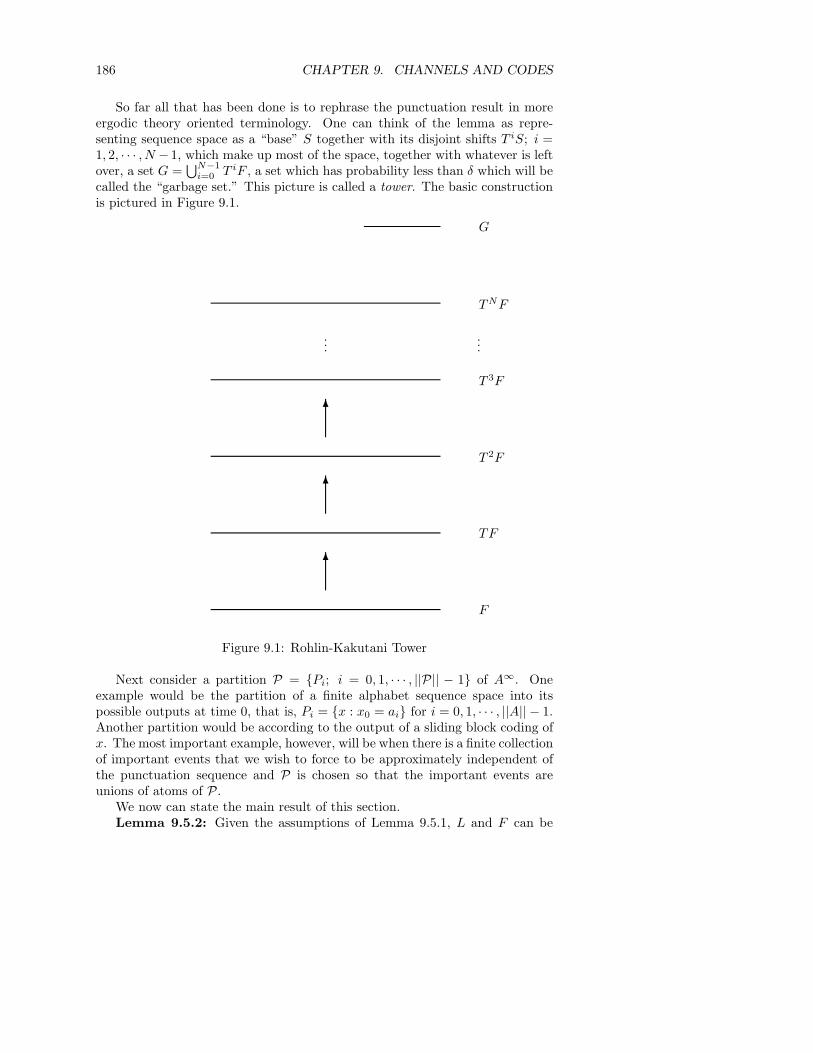
186 CHAPTER 9. CHANNELS AND CODES
So far all that has been done is to rephrase the punctuation result in moreergodic theory oriented terminology. One can think of the lemma as repre-senting sequence space as a “base” S together with its disjoint shifts T iS; i =1, 2, · · · , N − 1, which make up most of the space, together with whatever is leftover, a set G =
⋃N−1i=0 T iF , a set which has probability less than δ which will be
called the “garbage set.” This picture is called a tower. The basic constructionis pictured in Figure 9.1.
F
6
TF
6
T 2F
6
T 3F
......
TNF
G
Figure 9.1: Rohlin-Kakutani Tower
Next consider a partition P = Pi; i = 0, 1, · · · , ||P|| − 1 of A∞. Oneexample would be the partition of a finite alphabet sequence space into itspossible outputs at time 0, that is, Pi = x : x0 = ai for i = 0, 1, · · · , ||A|| − 1.Another partition would be according to the output of a sliding block coding ofx. The most important example, however, will be when there is a finite collectionof important events that we wish to force to be approximately independent ofthe punctuation sequence and P is chosen so that the important events areunions of atoms of P.
We now can state the main result of this section.Lemma 9.5.2: Given the assumptions of Lemma 9.5.1, L and F can be
9.5. THE ROHLIN-KAKUTANI THEOREM 187
chosen so that in addition to properties (A)-(C) it is also true that
(D)µ(Pi|F ) = µ(Pi|T lF ); l = 1, 2, · · · , N − 1, (9.11)
µ(Pi|F ) = µ(Pi|N−1⋃k=0
T kF ) (9.12)
andµ(Pi
⋂F ) ≤ 1
Nµ(Pi). (9.13)
Comment: Eq. (9.13) can be interpreted as stating that Pi and F areapproximately independent since 1/N is approximately the probability of F .Only the upper bound is stated as it is all we need. Eq. (9.11) also implies thatµ(Pi
⋂F ) is bound below by (µ(Pi) − δ)µ(F ).
Proof: Eq. (9.12) follows from (9.11) since
µ(Pi|N−1⋃l=0
T lF ) =µ(Pi
⋂ ⋃N−1l=0 T lF )
µ(⋃N−1
l=0 T lF )=
∑N−1l=0 µ(Pi
⋂T lF )∑N−1
l=0 µ(T lF )
=∑N−1
l=0 µ(Pi|T lF )µ(T lF )Nµ(F )
=1N
N−1∑l=0
µ(Pi|T lF )µ(F ).
Eq. (9.13) follows from (9.12) since
µ(Pi
⋂F ) = µ(Pi|F )µ(F ) = µ(Pi|
N−1⋃k=0
T kF )µ(F )
= µ(Pi|N−1⋃k=0
T kF )1N
µ(N−1⋃k=0
T kF )),
since the T kF are disjoint and have equal probability,
=1N
µ(Pi
⋂ N−1⋃k=0
T kF ) ≤ 1N
µ(Pi).
The remainder of this section is devoted to proving (9.11). We begin by review-ing and developing some needed notation.
Given a partition P, we define the label function
labelP(x) =||P||−1∑
i=0
i1Pi(x),
where as usual 1P is the indicator function of a set P . Thus the label of asequence is simply the index of the atom of the partition into which it falls.
188 CHAPTER 9. CHANNELS AND CODES
As P partitions the input space into which sequences belong to atoms of P,T−iP partitions the space according to which shifted sequences T ix belong toatoms of P, that is, x ∈ T−iPl ∈ T−iP is equivalent to T ix ∈ Pl and hencelabelP(T ix) = l. The join
PN =N−1∨i=0
T−iP
partitions the space into sequences sharing N labels in the following sense: Eachatom Q of PN has the form
Q = x : labelP(x) = k0, labelP(Tx) = k1, · · · , labelP(TN−1x) = kN − 1
for some N tuple of integers k = (k0, · · · , kN − 1). For this reason we will indexthe atoms of PN as Qk. Thus PN breaks up the sequence space into groups ofsequences which have the same labels for N shifts.
We first construct using Lemma 9.5.1 a huge tower of size KN >> N , theheight of the tower to be produced for this lemma. Let S denote the base ofthis original tower and let ε by the probability of the garbage set. This heightKN tower with base S will be used to construct a new tower of height N anda base F with the additional desired property. First consider the restriction ofthe partition PN to F defined by PN
⋂F = Qk
⋂F ; all KN -tuples k with
coordinates taking values in 0, 1, · · · , ||P||−1. PN⋂
F divides up the originalbase according to the labels of NK shifts of base sequences. For each atomQk
⋂F in this base partition, the sets T l(Qk
⋂F ); k = 0, 1, · · · ,KN − 1 are
disjoint and together form a column of the tower T lF ; k = 0, 1, · · · ,KN − 1.A set of the form T l(Qk
⋂F ) is called the lth level of the column containing it.
Observe that if y ∈ T l(Qk
⋂F ), then y = T lu for some u ∈ Qk
⋂F and T lu has
label kl. Thus we consider kl to be the label of the column level T l(Qk
⋂F ).
This complicated structure of columns and levels can be used to recover theoriginal partition by
Pj =⋃
l,k:kl=j
T l(Qk
⋂F )
⋂(Pj
⋂G), (9.14)
that is, Pj is the union of all column levels with label j together with that partof Pj in the garbage. We will focus on the pieces of Pj in the column levels asthe garbage has very small probability.
We wish to construct a new tower with base F so that the probability of Pi
for any of N shifts of F is the same. To do this we form F dividing each columnof the original tower into N equal parts. We collect a group of these parts toform F so that F will contain only one part at each level, the N shifts of F willbe disjoint, and the union of the N shifts will almost contain all of the originaltower. By using the equal probability parts the new base will have conditionalprobabilities for Pj given T l equal for all l, as will be shown.
Consider the atom Q = Qk
⋂S in the partition PN
⋂S of the base of the
original tower. If the source is aperiodic in the sense of placing zero probability
9.5. THE ROHLIN-KAKUTANI THEOREM 189
on individual sequences, then the set Q can be divided into N disjoint sets ofequal probability, say W0,W1, · · · ,WN−1. Define the set FQ by
FQ = ((K−2)N⋃
i=0
T iNW0)⋃
((K−2)N⋃
i=0
T 1+iNW1)⋃
· · · ((K−2)N⋃
i=0
TN−1+iNWN−1) =N−1⋃l=0
(K−2)N⋃i=0
T l+iNWl.
FQ contains (K−2) N shifts of W0, of TW1, · · · of T lWl, · · · and of TN−1WN−1.Because it only takes N -shifts of each small set and because it does not includethe top N levels of the original column, shifting FQ fewer than N times causesno overlap, that is, T lFQ are disjoint for j = 0, 1, · · · , N −1. The union of thesesets contains all of the original column of the tower except possibly portions ofthe top and bottom N −1 levels (which the construction may not include). Thenew base F is now defined to be the union of all of the FQk
⋂S . The sets T lF
are then disjoint (since all the pieces are) and contain all of the levels of theoriginal tower except possibly the top and bottom N − 1 levels. Thus
µ(N−1⋃l=0
T lF ) ≥ µ((K−1)N−1⋃
i=N
T iS) =(K−1)N−1∑
i=N
µ(S)
≥ K − 21 − ε
KN=
1 − ε
N− 2
KN.
by choosing ε = δ/2 and K large this can be made larger than 1 − δ. Thus thenew tower satisfies conditions (A)-(C) and we need only verify the new condition(D), that is, (9.11). We have that
µ(Pi|T lF ) =µ(Pi
⋂T lF )
µ(F ).
Since the denominator does not depend on l, we need only show the numeratordoes not depend on l. From (9.14) applied to the original tower we have that
µ(Pi
⋂T lF ) =
∑j,k:kj=i
µ(T j(Qk
⋂S)
⋂T lF ),
that is, the sum over all column levels (old tower) labeled i of the probabilityof the intersection of the column level and the lth shift of the new base F . Theintersection of a column level in the jth level of the original tower with any shiftof F must be an intersection of that column level with the jth shift of one ofthe sets W0, · · · ,WN−1 (which particular set depends on l). Whichever set ischosen, however, the probability within the sum has the form
µ(T j(Qk
⋂S)
⋂T lF ) = µ(T j(Qk
⋂S)
⋂T jWm)
190 CHAPTER 9. CHANNELS AND CODES
= µ((Qk
⋂S)
⋂Wm) = µ(Wm),
where the final step follows since Wm was originally chosen as a subset of Qk
⋂S.
Since these subsets were all chosen to have equal probability, this last probabilitydoes not depend on m and hence on l and
µ(T j(Qk
⋂S)
⋂T lF ) =
1N
µ(Qk
⋂S)
and henceµ(Pi
⋂T lF ) =
∑j,k:kj=i
1N
µ(Qk
⋂S),
which proves (9.11) since there is no dependence on l. This completes the proofof the lemma. 2
Chapter 10
Distortion
10.1 Introduction
We now turn to quantification of various notions of the distortion between ran-dom variables, vectors and processes. A distortion measure is not a “measure”in the sense used so far; it is an assignment of a nonnegative real number whichindicates how bad an approximation one symbol or random object is of another;the smaller the distortion, the better the approximation. If the two objects cor-respond to the input and output of a communication system, then the distortionprovides a measure of the performance of the system. Distortion measures neednot have metric properties such as the triangle inequality and symmetry, butsuch properties can be exploited when available. We shall encounter severalnotions of distortion and a diversity of applications, with eventually the mostimportant application being a measure of the performance of a communica-tions system by an average distortion between the input and output. Otherapplications include extensions of finite memory channels to channels which ap-proximate finite memory channels and different characterizations of the optimalperformance of communications systems.
10.2 Distortion and Fidelity Criteria
Given two measurable spaces (A,BA) and (B,BB), a distortion measure onA × B is a nonnegative measurable mapping ρ : A × B → [0,∞) which assignsa real number ρ(x, y) to each x ∈ A and y ∈ B which can be thought of as thecost of reproducing x and y. The principal practical goal is to have a number bywhich the goodness or badness of communication systems can be compared. Forexample, if the input to a communication system is a random variable X ∈ Aand the output is Y ∈ B, then one possible measure of the quality of the systemis the average distortion Eρ(X,Y ). Ideally one would like a distortion measureto have three properties:
191
192 CHAPTER 10. DISTORTION
• It should be tractable so that one can do useful theory.
• It should be computable so that it can be measured in real systems.
• It should be subjectively meaningful in the sense that small (large) dis-tortion corresponds to good (bad) perceived quality.
Unfortunately these requirements are often inconsistent and one is forcedto compromise between tractability and subjective significance in the choice ofdistortion measures. Among the most popular choices for distortion measuresare metrics or distances, but many practically important distortion measuresare not metrics, e.g., they are not symmetric in their arguments or they do notsatisfy a triangle inequality. An example of a metric distortion measure thatwill often be emphasized is that given when the input space A is a Polish space,a complete separable metric space under a metric ρ, and B is either A itselfor a Borel subset of A. In this case the distortion measure is fundamental tothe structure of the alphabet and the alphabets are standard since the space isPolish.
Suppose next that we have a sequence of product spaces An and Bn forn = 1, 2, · · ·. A fidelity criterion ρn, n = 1, 2, · · · is a sequence of distortionmeasures on An × Bn. If one has a pair random process, say Xn, Yn, then itwill be of interest to find conditions under which there is a limiting per symboldistortion in the sense that
ρ∞(x, y) = limn→∞
1n
ρn(xn, yn)
exists. As one might guess, the distortion measures in the sequence often areinterrelated. The simplest and most common example is that of an additive orsingle-letter fidelity criterion which has the form
ρn(xn, yn) =n−1∑i=0
ρ1(xi, yi).
Here if the pair process is AMS, then the limiting distortion will exist andit is invariant from the ergodic theorem. By far the bulk of the informationtheory literature considers only single-letter fidelity criteria and we will sharethis emphasis. We will point out, however, other examples where the basicmethods and results apply. For example, if ρn is subadditive in the sense that
ρn(xn, yn) ≤ ρk(xk, yk) + ρn−k(xn−kk , yn−k
k ),
then stationarity of the pair process will ensure that n−1ρn converges from thesubadditive ergodic theorem. For example, if d is a distortion measure on A×B,then
ρn(xn, yn) =
(n−1∑i=0
d(xi, yi)p
)1/p
10.3. PERFORMANCE 193
for p > 1 is subadditive from Minkowski’s inequality.As an even simpler example, if d is a distortion measure on A×B, then the
following fidelity criterion converges for AMS pair processes:
1n
ρn(xn, yn) =1n
n−1∑i=0
f(d(xi, yi)).
This form often arises in the literature with d being a metric and f being anonnegative nondecreasing function (sometimes assumed convex).
The fidelity criteria introduced here all are context-free in that the distortionbetween n successive input/output samples of a pair process does not dependon samples occurring before or after these n-samples. Some work has beendone on context-dependent distortion measures (see, e.g., [93]), but we do notconsider their importance sufficient to merit the increased notational and tech-nical difficulties involved. Hence we shall consider only context-free distortionmeasures.
10.3 Performance
As a first application of the notion of distortion, we define a performance mea-sure of a communication system. Suppose that we have a communication system[µ, f, ν, g] such that the overall input/output process is Xn, Xn. For the mo-ment let p denote the corresponding distribution. Then one measure of thequality (or rather the lack thereof) of the communication system is the longterm time average distortion per symbol between the input and output as de-termined by the fidelity criterion. Given two sequences x and x and a fidelitycriterion ρn; n = 1, 2, · · ·, define the limiting sample average distortion or se-quence distortion by
ρ∞(x, y) = lim supn→∞
1n
ρn(xn, yn).
Define the performance of a communication system by the expected value of thelimiting sample average distortion:
∆(µ, f, ν, g) = Epρ∞ = Ep
(lim sup
n→∞
1n
ρn(Xn, Xn))
. (10.1)
We will focus on two important special cases. The first is that of AMS sys-tems and additive fidelity criteria. A large majority of the information theoryliterature is devoted to additive distortion measures and this bias is reflectedhere. We also consider the case of subadditive distortion measures and systemsthat are either two-sided and AMS or are one-sided and stationary. Unhappilythe overall AMS one-sided case cannot be handled as there is not yet a subad-ditive ergodic theorem for that case. In all of these cases we have that if ρ1 is
194 CHAPTER 10. DISTORTION
integrable with respect to the stationary mean process p, then
ρ∞(x, y) = limn→∞
1n
ρn(xn, yn); p − a.e., (10.2)
and ρ∞ is an invariant function of its two arguments, i.e.,
ρ∞(TAx, TAy) = ρ∞(x, y); p − a.e.. (10.3)
When a system and fidelity criterion are such that (10.2) and (10.3) aresatisfied we say that we have a convergent fidelity criterion. We henceforthmake this assumption.
Since ρ∞ is invariant, we have from Lemma 6.3.1 of [50] that
∆ = Epρ∞ = Epρ∞. (10.4)
If the fidelity criterion is additive, then we have from the stationarity of pthat the performance is given by
∆ = Epρ1(X0, Y0). (10.5)
If the fidelity criterion is subadditive, then this is replaced by
∆ = infN
1N
EpρN (XN , Y N ). (10.6)
Assume for the remainder of this section that ρn is an additive fidelity crite-rion. Suppose now that we now that p is N -stationary; that is, if T = TA × TA
denotes the shift on the input/output space AT × AT , then the overall processis stationary with respect to TN . In this case
∆ =1N
EρN (XN , XN ). (10.7)
We will have this N stationarity, for example, if the source and channel arestationary and the coders are N -stationary, e.g., are length N -block codes. Moregenerally, the source could be N -stationary, the first sequence coder (N,K)-stationary, the channel K-stationary (e.g., stationary), and the second sequencecoder (K,N)-stationary.
We can also consider the behavior of the N -shift more generally when thesystem is only AMS This will be useful when considering block codes. Supposenow that p is AMS with stationary mean p. Then from Theorem 7.3.1 of [50],p is also T N -AMS with an N -stationary mean, say pN . Applying the ergodictheorem to the N shift then implies that if ρN is pN -integrable, then
limn→∞
1n
n−1∑i=0
ρN (xNiN , yN
iN ) = ρ(N)∞ (10.8)
exists pN (and hence also p) almost everywhere. In addition, ρ(N)∞ is N -invariant
andEpρ
(N)∞ = EpN
ρ(N)∞ = EpN
ρN (XN , Y N ). (10.9)
10.4. THE RHO-BAR DISTORTION 195
Comparison of (10.2) and (10.9) shows that ρ(N)∞ = Nρ∞ p-a.e. and hence
∆ =1N
EpNρN (XN , Y N ) =
1N
Epρ(N)∞ = Epρ1(X0, Y0). (10.10)
Given a notion of the performance of a communication system, we can nowdefine the optimal performance achievable for trying to communicate a givensource Xn with distribution µ over a channel ν: Suppose that E is some classof sequence coders f : AT → BT . For example, E might consist of all sequencecoders generated by block codes with some constraint or by finite-length slidingblock codes. Similarly let D denote a class of sequence coders g : B′T → AT .Define the optimal performance theoretically achievable or OPTA function forthe source µ, channel ν, and code classes E and D by
∆∗(µ, ν, E ,D) = inff∈E,g∈D
∆([µ, f, ν, g]). (10.11)
The goal of the coding theorems of information theory is to relate the OPTAfunction to (hopefully) computable functions of the source and channel.
10.4 The rho-bar distortion
In the previous sections it was pointed out that if one has a distortion measureρ on two random objects X and Y and a joint distribution on the two randomobjects (and hence also marginal distributions for each), then a natural notion ofthe difference between the processes or the poorness of their mutual approxima-tion is the expected distortion Eρ(X,Y ). We now consider a different question:What if one does not have a joint probabilistic description of X and Y , butinstead knows only their marginal distributions. What then is a natural no-tion of the distortion or poorness of approximation of the two random objects?In other words, we previously measured the distortion between two randomvariables whose stochastic connection was determined, possibly by a channel, acode, or a communication system. We now wish to find a similar quantity forthe case when the two random objects are only described as individuals. Onepossible definition is to find the smallest possible distortion in the old senseconsistent with the given information, that is, to minimize Eρ(X,Y ) over alljoint distributions consistent with the given marginal distributions. Note thatthis will necessarily give a lower bound to the distortion achievable when anyspecific joint distribution is specified.
To be precise, suppose that we have random variables X and Y with distri-butions PX and PY and alphabets A and B, respectively. Let ρ be a distortionmeasure on A × B. Define the ρ-distortion (pronounced ρ-bar) between therandom variables X and Y by
ρ(PX , PY ) = infp∈P
Epρ(X,Y ),
Where P = P(PX , PY ) is the collection of all measures on (A×B,BA ×BB)with PX and PY as marginals; that is,
p(A × F ) = PY (F ); F ∈ BB ,
196 CHAPTER 10. DISTORTION
andp(G × B) = PX(G); G ∈ BA.
Note that P is not empty since, for example, it contains the product measurePX × PY .
Levenshtein [94] and Vasershtein [144] studied this quantity for the specialcase where A and B are the real line and ρ is the Euclidean distance. When asin their case the distortion is a metric or distance, the ρ-distortion is called theρ-distance. Ornstein [116] developed the distance and many of its propertiesfor the special case where A and B were common discrete spaces and ρ was theHamming distance. In this case the ρ-distance is called the d-distance. R. L.Dobrushin has suggested that because of the common suffix in the names of itsoriginators, this distance between distributions should be called the shtein orstein distance.
The ρ-distortion can be extended to processes in a natural way. Supposenow that Xn is a process with process distribution mX and that Yn is aprocess with process distribution mY . Let PXn and PY n denote the inducedfinite dimensional distributions. A fidelity criterion provides the distortion ρn
between these n dimensional alphabets. Let ρn denote the corresponding ρdistortion between the n dimensional distributions. Then
ρ(mX ,mY ) = supn
1n
ρn(PXn , PY n);
that is, the ρ-distortion between two processes is the maximum of the ρ-distortionsper symbol between n-tuples drawn from the process. The properties of the ρdistance are developed in [57] [119] and a detailed development may be foundin [50] . The following theorem summarizes the principal properties.
Theorem 10.4.1: Suppose that we are given an additive fidelity criterion ρn
with a pseudo-metric per-letter distortion ρ1 and suppose that both distributionsmX and mY are stationary and have the same standard alphabet. Then
(a) limn→∞ n−1ρn(PXn , PY n) exists and equals supn n−1ρn(PXn , PY n).
(b) ρn and ρ are pseudo-metrics. If ρ1 is a metric, then ρn and ρ are metrics.
(c) If mX and mY are both i.i.d., then ρ(mX ,mY ) = ρ1(PX0 , PY0).
(d) Let Ps = Ps(mX ,mY ) denote the collection of all stationary distributionspXY having mX and mY as marginals, that is, distributions on Xn, Ynwith coordinate processes Xn and Yn having the given distributions.Define the process distortion measure ρ′
ρ′(mX ,mY ) = infpXY ∈Ps
EpXYρ(X0, Y0).
Thenρ(mX ,mY ) = ρ′(mX ,mY );
that is, the limit of the finite dimensional minimizations is given by aminimization over stationary processes.
10.5. D-BAR CONTINUOUS CHANNELS 197
(e) Suppose that mX and mY are both stationary and ergodic. Define Pe =Pe(mX ,mY ) as the subset of Ps containing only ergodic processes, then
ρ(mX ,mY ) = infpXY ∈Pe
EpXYρ(X0, Y0),
(f) Suppose that mX and mY are both stationary and ergodic. Let GX denotea collection of generic sequences for mX in the sense of Section 8.3 of [50].Generic sequences are those along which the relative frequencies of a set ofgenerating events all converge and hence by measuring relative frequencieson generic sequences one can deduce the underlying stationary and ergodicmeasure that produced the sequence. An AMS process produces genericsequences with probability 1. Similarly let GY denote a set of genericsequences for mY . Define the process distortion measure
ρ′′(mX ,mY ) = infx∈GX ,y∈GY
lim supn→∞
1n
n−1∑i=0
ρ1(x0, y0).
Thenρ(mX ,mY ) = ρ′′(mX ,mY );
that is, the ρ distance gives the minimum long term time average distortionobtainable between generic sequences from the two sources.
(g) The infima defining ρn and ρ′ are actually minima.
10.5 d-bar Continuous Channels
We can now generalize some of the notions of channels by using the ρ-distanceto weaken the definitions. The first definition is the most important for chan-nel coding applications. We now confine interest to the d-bar distance, theρ-distance for the special case of the Hamming distance:
ρ1(x, y) = d1(x, y) =
0 if x = y1 if x 6= y.
Suppose that [A, ν,B] is a discrete alphabet channel and let νnx denote the
restriction of the channel to Bn, that is, the output distribution on Y n givenan input sequence x. The channel is said to be d-continuous if for any ε > 0there is an n0 such that for all n > n0 dn(νn
x , νnx′) ≤ ε whenever xi = x′
i fori = 0, 1, · · · , n. Alternatively, ν is d-continuous if
lim supn→∞
supan∈An
supx,x′∈c(an)
dn(νnx , νn
x′) = 0,
where c(an) is the rectangle defined as all x with xi = ai; i = 0, 1, · · · , n − 1.d-continuity implies the distributions on output n-tuples Y n given two inputsequences are very close provided that the input sequences are identical over the
198 CHAPTER 10. DISTORTION
same time period and that n is large. This generalizes the notions of 0 or finiteinput memory and anticipation since the distributions need only approximateeach other and do not have to be exactly the same.
More generally we could consider ρ-continuous channels in a similar manner,but we will focus on the simpler discrete d-continuous channel.
d-continuous channels possess continuity properties that will be useful forproving block and sliding block coding theorems. They are “continuous” in thesense that knowing the input with sufficiently high probability for a sufficientlylong time also specifies the output with high probability. The following twolemmas make these ideas precise.
Lemma 10.5.1: Suppose that x, x ∈ c(an) and
d(νnx , νn
x ) ≤ δ2.
This is the case, for example, if the channel is d continuous and n is chosensufficiently large. Then
νnx (Gδ) ≥ νn
x (G) − δ
and henceinf
x∈c(an)νn
x (Gδ) ≥ supx∈c(an)
νnx (G) − δ.
Proof: From Theorem 10.4.1 the infima defining the d distance are actuallyminima and hence there is a pmf p on Bn × Bn such that∑
bn∈Bn
p(yn, bn) = νnx (yn)
and ∑bn∈Bn
p(bn, yn) = νnx (yn);
that is, p has νnx and νn
x as marginals, and
1n
Epdn(Y n, Y n) = d(νnx , νn
x ).
Using the Markov inequality we can write
νnx (Gδ) = p(Y n ∈ Gδ)
≥ p(Y n ∈ G and dn(Y n, Y n) ≤ nδ) = 1 − p(Y n 6∈ G or dn(Y n, Y n) > nδ)
≥ 1 − p(Y n 6∈ G) − p(dn(Y n, Y n) > nδ) ≥ νnx (G) − 1
δE(n−1dn(Y n, Y n))
≥ νnx (G) − δ
proving the first statement. The second statement follows from the first. 2
Next suppose that [G,µ, U ] is a stationary source, f is a stationary encoderwhich could correspond to a finite length sliding block encoder or to an infinite
10.5. D-BAR CONTINUOUS CHANNELS 199
length one, ν is a stationary channel, and g is a length m sliding block decoder.The probability of error for the resulting hookup is defined by
Pe(µ, ν, f, g) = Pr(U0 6= U0) = µν(E) =∫
dµ(u)νf(u)(Eu),
where E is the error event u, y : u0 6= gm(Y−qm) and Eu = y : (u, y) ∈ E isthe section of E at u.
Lemma 10.5.2: Given a stationary channel ν, a stationary source [G,µ, U ],a length m sliding block decoder, and two encoders f and φ, then for any positiveinteger r
|Pe(µ, ν, f, g) − Pe(µ, ν, φ, g)|
≤ m
r+ r Pr(f 6= φ) + m max
ar∈Arsup
x,x′∈c(ar)
dr(νrx, νr
x′).
Proof: Define Λ = u : f(u) = φ(u) and
Λr = u : f(T iu) = φ(T iu); i = 0, 1 · · · , r − 1 =r−1⋂i=0
T iΛ.
From the union bound
µ(Λcr) ≤ rµ(Λc) = rPr(f 6= φ). (10.12)
From stationarity, if g = gm(Y m−q) then
Pe(µ, ν, f, g) =∫
dµ(u)νf(u)(y : gm(ym−q) 6= u0)
=1r
r−1∑i=0
∫dµ(u)νf(u)(y : gm(ym
i−q) 6= u0)
≤ m
r+
1r
r−q∑i=q
∫Λr
dµ(u)νrf(u)(y
r : gm(ymi−q) 6= ui) + µ(Λc
r). (10.13)
Fix u ∈ Λr and let pu yield dr(νrf(u),φ(u)); that is,
∑wr pu(yr, wr) = νr
f(u)(yr),∑
yr pu(yr, wr) = νrφ(u)(w
r), and
1r
r−1∑i=0
pu(yr, wr : yi 6= wi) = dr(νrf(u),φ(u)). (10.14)
We have that
1r
r−q∑i=q
νrf(u)(y
r : gm(ymi−q) 6= ui) =
1r
r−q∑i=q
pu(yr, wr : gm(ymi−q) 6= ui)
200 CHAPTER 10. DISTORTION
≤ 1r
r−q∑i=q
pu(yr, wr : gm(ymi−q) 6= wm
i−q) +1r
r−q∑i=q
pu(yr, wr : gm(wmi−q) 6= ui)
≤ 1r
r−q∑i=q
pu(yr, wr : yri−q 6= wr
i−q) + Pe(µ, ν, φ, g)
≤ 1r
r−q∑i=q
i−q+m∑j=i−q
pu(yr, wr : yj 6= wj) + Pe(µ, ν, φ, g)
≤ mdr(νrf(u), ν
rφ(u)) + Pe(µ, ν, φ, g),
which with (10.12)-(10.14) proves the lemma. 2
The following corollary states that the probability of error using sliding blockcodes over a d-continuous channel is a continuous function of the encoder asmeasured by the metric on encoders given by the probability of disagreement ofthe outputs of two encoders.
Corollary 10.5.1: Given a stationary d-continuous channel ν and a finitelength decoder gm : Bm → A, then given ε > 0 there is a δ > 0 so that if f andφ are two stationary encoders such that Pr(f 6= g) ≤ δ, then
|Pe(µ, ν, f, g) − Pe(µ, ν, φ, g)| ≤ ε.
Proof: Fix ε > 0 and choose r so large that
maxar
supx,x′∈c(ar)
dr(νrx, νr
x′) ≤ ε
3m,
m
r≤ ε
3,
and choose δ = ε/(3r). Then Lemma 10.5.2 implies that
|Pe(µ, ν, f, g) − Pe(µ, ν, φ, g)| ≤ ε. 2
Given an arbitrary channel [A, ν,B], we can define for any block lengthN a closely related CBI channel [A, ν, B] as the CBI channel with the sameprobabilities on output N -blocks, that is, the same conditional probabilities forY N
kN given x, but having conditionally independent blocks. We shall call ν theN -CBI approximation to ν. A channel ν is said to be conditionally almost blockindependent or CABI if given ε there is an N0 such that for any N ≥ N0 thereis an M0 such that for any x and any N -CBI approximation ν to ν
d(νMx , νM
x ) ≤ ε, all M ≥ M0,
where νMx denotes the restriction of νx to BN
B , that is, the output distribution onY N given x. A CABI channel is one such that the output distribution is close (ina d sense) to that of the N -CBI approximation provided that N is big enough.CABI channels were introduced by Neuhoff and Shields [110] who provided
10.6. THE DISTORTION-RATE FUNCTION 201
several examples alternative characterizations of the class. In particular theyshowed that finite memory channels are both d-continuous and CABI. Theirprincipal result, however, requires the notion of the d distance between channels.Given two channels [A, ν,B] and [A, ν′, B], define the d distance between thechannels to be
d(ν, ν′) = lim supn→∞
supx
d(νnx , ν′N
x ).
Neuhoff and Shields [110] showed that the class of CABI channels is exactlythe class of primitive channels together with the d limits of such channels.
10.6 The Distortion-Rate Function
We close this chapter on distortion, approximation, and performance with theintroduction and discussion of Shannon’s distortion-rate function. This function(or functional) of the source and distortion measure will play a fundamental rolein evaluating the OPTA functions. In fact, it can be considered as a form ofinformation theoretic OPTA. Suppose now that we are given a source [A,µ]and a fidelity criterion ρn; n = 1, 2, · · · defined on A × A, where A is calledthe reproduction alphabet. Then the Shannon distortion rate function (DRF) isdefined in terms of a nonnegative parameter called rate by
D(R,µ) = lim supN→∞
1N
DN (R,µN )
whereDN (R,µN ) = inf
pN∈RN (R,µN )EpN ρN (XN , Y N ),
where RN (R,µN ) is the collection of all distributions pN for the coordinaterandom vectors XN and Y N on the space (AN × AN , BN
A × BNA
) with theproperties that
(1) pN induces the given marginal µN ; that is, pN (AN × F ) = µN (F ) for allF ∈ BN
A , and
(2) the mutual information satisfies
1N
IpN (XN ; XN ) ≤ R.
If RN (R,µN ) is empty, then DN (R,µN ) is ∞. DN is called the Nth orderdistortion-rate function.
Lemma 10.6.1: DN (R,µ) and D(R,µ) are nonnegative convex⋃
functionsof R and hence are continuous in R for R > 0.
Proof: Nonnegativity is obvious from the nonnegativity of distortion. Sup-pose that pi ∈ RN (Ri, µ
N ); i = 1, 2 yields
EpiρN (XN , Y N ) ≤ DN (Ri, µ) + ε.
202 CHAPTER 10. DISTORTION
From Corollary 5.5.5 mutual information is a convex⋃
function of the condi-tional distribution and hence if p = λp1 + (1 − λ)p2, then
Ip ≤ λIp1 + (1 − λ)Ip2 ≤ λR1 + (1 − λ)R2
and hence p ∈ RN (λR1 + (1 − λ)R2) and therefore
DN (λR1 + (1 − λ)R2) ≤ EpρN (XN , Y N )
= λEp1ρN (XN , Y N ) + (1 − λ)Ep2ρN (XN , Y N )
≤ λDN (R1, µ) + (1 − λ)DN (R2, µ).
Since D(R,µ) is the limit of DN (R,µ), it too is convex. It is well known fromreal analysis that convex functions are continuous except possibly at their endpoints. 2
The following lemma shows that when the underlying source is stationaryand the fidelity criterion is subadditive (e.g., additive), then the limit definingD(R,µ) is an infimum.
Lemma 10.6.2: If the source µ is stationary and the fidelity criterion issubadditive, then
D(R,µ) = limN→∞
DN (R,µ) = infN
1N
DN (R,µ).
Proof: Fix N and n < N and let pn ∈ Rn(R,µn) yield
Epnρn(Xn, Y n) ≤ Dn(R,µn) +ε
2
and let pN−n ∈ RN−n(R,µN−n) yield
EpN−nρN−n(XN−n, Y N−n) ≤ DN−n(R,µN−n) +ε
2.
pn together with µn implies a regular conditional probability q(F |xn), F ∈ BnA.
Similarly pN−n and µN−n imply a regular conditional probability r(G|xN−n).Define now a regular conditional probability t(·|xN ) by its values on rectanglesas
t(F × G|xN ) = q(F |xn)r(G|xN−nn ); F ∈ Bn
A, G ∈ BN−n
A.
Note that this is the finite dimensional analog of a block memoryless channelwith two blocks. Let pN = µN t be the distribution induced by µ and t. Thenexactly as in Lemma 9.4.2 we have because of the conditional independence that
IpN (XN ;Y N ) ≤ IpN (Xn;Y n) + IpN (XN−nn ;Y N−n
n )
and hence from stationarity
IpN (XN ;Y N ) ≤ Ipn(Xn;Y n) + IpN−n(XN−n;Y N−n)
10.6. THE DISTORTION-RATE FUNCTION 203
≤ nR + (N − n)R = NR
so that pN ∈ RN (R,µN ). Thus
DN (R,µN ) ≤ EpN ρN (XN , Y N ) ≤ EpN
(ρn(Xn, Y n) + ρN−n(XN−n
n , Y N−nn )
)= Epnρn(Xn, Y n) + EpN−nρN−n(XN−n, Y N−n)
≤ Dn(R,µn) + DN−n(R,µN−n) + ε.
Thus since ε is arbitrary we have shown that if dn = Dn(R,µn), then
dN ≤ dn + dN−n; n ≤ N ;
that is, the sequence dn is subadditive. The lemma then follows immediatelyfrom Lemma 7.5.1 of [50]. 2
As with the ρ distance, there are alternative characterizations of the distortion-rate function when the process is stationary. The remainder of this section isdevoted to developing these results. The idea of an SBM channel will playan important role in relating nth order distortion-rate functions to the processdefinitions. We henceforth assume that the input source µ is stationary andwe confine interest to additive fidelity criteria based on a per-letter distortionρ = ρ1.
The basic process DRF is defined by
Ds(R,µ) = infp∈Rs(R,µ)
Epρ(X0, Y0),
where Rs(R,µ) is the collection of all stationary processes p having µ as aninput distribution and having mutual information rate Ip = Ip(X;Y ) ≤ R. Theoriginal idea of a process rate-distortion function was due to Kolmogorov andhis colleagues [87] [45] (see also [23]). The idea was later elaborated by Marton[101] and Gray, Neuhoff, and Omura [55].
Recalling that the L1 ergodic theorem for information density holds whenIp = I∗p ; that is, the two principal definitions of mutual information rate yieldthe same value, we also define the process DRF
D∗s(R,µ) = inf
p∈R∗s(R,µ)
Epρ(X0, Y0),
where R∗s(R,µ) is the collection of all stationary processes p having µ as an
input distribution, having mutual information rate Ip ≤ R, and having Ip = I∗p .If µ is both stationary and ergodic, define the corresponding ergodic processDRF’s by
De(R,µ) = infp∈Re(R,µ)
Epρ(X0, Y0),
D∗e(R,µ) = inf
p∈R∗e(R,µ)
Epρ(X0, Y0),
where Re(R,µ) is the subset of Rs(R,µ) containing only ergodic measures andR∗
e(R,µ) is the subset of R∗s(R,µ) containing only ergodic measures.
204 CHAPTER 10. DISTORTION
Theorem 10.6.1: Given a stationary source which possesses a referenceletter in the sense that there exists a letter a∗ ∈ A such that
Eµρ(X0, a∗) ≤ ρ∗ < ∞. (10.15)
Fix R > 0. If D(R,µ) < ∞, then
D(R,µ) = Ds(R,µ) = D∗s(R,µ).
If in addition µ is ergodic, then also
D(R,µ) = De(R,µ) = D∗e(R,µ).
The proof of the theorem depends strongly on the relations among distortionand mutual information for vectors and for SBM channels. These are statedand proved in the following lemma, the proof of which is straightforward butsomewhat tedious. The theorem is proved after the lemma.
Lemma 10.6.3: Let µ be the process distribution of a stationary sourceXn. Let ρn; n = 1, 2, · · · be a subadditive (e.g., additive) fidelity criterion.Suppose that there is a reference letter a∗ ∈ A for which (10.15) holds. Let pN bea measure on (AN×AN , BN
A ×BNA
) having µN as input marginal; that is, pN (F×AN ) = µN (F ) for F ∈ BN
A . Let q denote the induced conditional probabilitymeasure; that is, qxN (F ), xN ∈ AN , F ∈ BN
A, is a regular conditional probability
measure. (This exists because the spaces are standard.) We abbreviate thisrelationship as pN = µNq. Let XN , Y N denote the coordinate functions onAN × AN and suppose that
EpN
1N
ρN (XN , Y N ) ≤ D (10.16)
and1N
IpN (XN ;Y N ) ≤ R. (10.17)
If ν is an (N, δ) SBM channel induced by q as in Example 9.4.11 and if p = µνis the resulting hookup and Xn, Yn the input/output pair process, then
1N
EpρN (XN , Y N ) ≤ D + ρ∗δ (10.18)
andIp(X;Y ) = I∗p (X;Y ) ≤ R; (10.19)
that is, the resulting mutual information rate of the induced stationary processsatisfies the same inequality as the vector mutual information and the resultingdistortion approximately satisfies the vector inequality provided δ is sufficientlysmall. Observe that if the fidelity criterion is additive, the (10.18) becomes
Epρ1(X0, Y0) ≤ D + ρ∗δ.
10.6. THE DISTORTION-RATE FUNCTION 205
Proof: We first consider the distortion as it is easier to handle. Since theSBM channel is stationary and the source is stationary, the hookup p is station-ary and
1n
Epρn(Xn, Y n) =1n
∫dmZ(z)Epz
ρn(Xn, Y n),
where pz is the conditional distribution of Xn, Yn given Zn. Note that theabove formula reduces to Epρ(X0, Y0) if the fidelity criterion is additive becauseof the stationarity. Given z, define Jn
0 (z) to be the collection of indices of zn forwhich zi is not in an N -cell. (See the discussion in Example 9.4.11.) Let Jn
1 (z)be the collection of indices for which zi begins an N -cell. If we define the eventG = z : z0 begins an N − cell, then i ∈ Jn
1 (z) if T iz ∈ G. From Corollary9.4.3 mZ(G) ≤ N−1. Since µ is stationary and Xn and Zn are mutuallyindependent,
nEpzρn(Xn, Y n) ≤
∑i∈Jn
0 (z)
Epzρ(Xi, a
∗) + N∑
i∈Jn1 (z)
Epzρ(XN
i , Y Ni )
=n−1∑i=0
1Gc(T iz)ρ∗ +n−1∑i=0
EpN ρN1G(T iz).
Since mZ is stationary, integrating the above we have that
Epρ1(X0, Y0) = ρ∗mZ(Gc) + NmZ(G)EpN ρN
≤ ρ∗δ + EpN ρN ,
proving (10.18).Let rm and tm denote asymptotically accurate quantizers on A and A; that
is, as in Corollary 6.2.1 define
Xn = rm(X)n = (rm(X0), · · · , rm(Xn−1))
and similarly define Y n = tm(Y )n. Then
I(rm(X)n; tm(Y )n) →m→∞
I(Xn;Y n)
andI(rm(X); tm(Y )) →
m→∞I∗(X;Y ).
We wish to prove that
I(X;Y ) = limn→∞
limm→∞
1n
I(rm(X)n; tm(Y )n)
= limm→∞
limn→∞
1n
I(rm(X)n; tm(Y )n). = I∗(X;Y )
Since I ≥ I∗, we must show that
limn→∞
limm→∞
1n
I(rm(X)n; tm(Y )n)
206 CHAPTER 10. DISTORTION
≤ limm→∞
limn→∞
1n
I(rm(X)n; tm(Y )n).
We have that
I(Xn; Y n) = I((Xn, Zn); Y n) − I(Zn, Y n|Xn)
and
I((Xn, Zn); Y n) = I(Xn; Y n|Zn) + I(Y n;Zn) = I(Xn; Y n|Zn)
since Xn and Zn are independent. Similarly,
I(Zn; Y n|Xn) = H(Zn|Xn) − H(Zn|Xn, Y n)
= H(Zn) − H(Zn|Xn, Y n) = I(Zn; (Xn, Y n)).
Thus we need to show that
limn→∞
limm→∞
(1n
I(rm(X)n; tm(Y )n|Zn) − 1n
I(Zn, (rm(X)n, tm(Y )n)))
≤ limm→∞
limn→∞
(1n
I(rm(X)n; tm(Y )n|Zn) − 1n
I(Zn, (rm(X)n, tm(Y )n)))
.
Since Zn has a finite alphabet, the limits of n−1I(Zn, (rm(X)n, tm(Y )n)) arethe same regardless of the order from Theorem 6.4.1. Thus I will equal I∗ if wecan show that
I(X;Y |Z) = limn→∞
limm→∞
1n
I(rm(X)n; tm(Y )n|Zn)
≤ limm→∞
limn→∞
1n
I(rm(X)n; tm(Y )n|Zn) = I∗(X;Y |Z). (10.20)
This we now proceed to do. From Lemma 5.5.7 we can write
I(rm(X)n; tm(Y )n|Zn) =∫
I(rm(X)n; tm(Y )n|Zn = zn) dPZn(zn).
Abbreviate I(rm(X)n; tm(Y )n|Zn = zn) to Iz(Xn; Y n). This is simply themutual information between Xn and Y n under the distribution for (Xn, Y n)given a particular random blocking sequence z. We have that
Iz(Xn; Y n) = Hz(Y n) − Hz(Y n|Xn).
Given z, let Jn0 (z) be as before. Let Jn
2 (z) denote the collection of all indices iof zi for which zi begins an N cell except for the final such index (which maybegin an N -cell not completed within zn). Thus Jn
2 (z) is the same as Jn1 (z)
except that the largest index in the latter collection may have been removed
10.6. THE DISTORTION-RATE FUNCTION 207
if the resulting N -cell was not completed within the n-tuple. We have usingstandard entropy relations that
Iz(Xn; Y n) ≥∑
i∈Jn0 (z)
(Hz(Yi|Y i) − Hz(Yi|Y i, Xi+1)
)
+∑
i∈Jn2 (z)
(Hz(Y N
i |Y i) − Hz(Y Ni |Y i, Xi+N )
). (10.21)
For i ∈ Jn0 (z), however, Yi is a∗ with probability one and hence
Hz(Yi|Y i) ≤ Hz(Yi) ≤ Hz(Yi) = 0
andHz(Yi|Y i, Xi+1) ≤ Hz(Yi) ≤ Hz(Yi) = 0.
Thus we have the bound
Iz(Xn; Y n) ≥∑
i∈Jn2 (z)
(Hz(Y N
i |Y i) − Hz(Y Ni |Y i, Xi+N )
).
=∑
i∈Jn2 (z)
(Iz(Y N
i ; (Y i, Xi + N)) − Iz(Y Ni ; Y i)
)
≥∑
i∈Jn2 (z)
(Iz(Y N
i ; XNi ) − Iz(Y N
i ; Y i))
, (10.22)
where the last inequality follows from the fact that I(U ; (V,W )) ≥ I(U ;V ).For i ∈ Jn
2 (z) we have by construction and the stationarity of µ that
Iz(XNi ; Y N
i ) = IpN (XN ; Y N ). (10.23)
As before let G = z : z0 begins an N − cell. Then i ∈ Jn2 (z) if T iz ∈ G and
i < n − N and we can write
1n
Iz(Xn; Y n) ≥ 1n
IpN (XN ; Y N )n−N−1∑
i=0
1G(T iz)
− 1n
n−N−1∑i=0
Iz(Y Ni ; Y i)1G(T iz).
All of the above terms are measurable functions of z and are nonnegative. Hencethey are integrable (although we do not yet know if the integral is finite) andwe have that
1n
I(Xn; Y n) ≥ Ipn(XN ; Y N )mZ(G)n − N
n
− 1n
n−N−1∑i=0
∫dmZ(z)Iz(Y N
i ; Y i)1G(T iz).
208 CHAPTER 10. DISTORTION
To continue we use the fact that since the processes are stationary, we canconsider it to be a two sided process (if it is one sided, we can imbed it in a twosided process with the same probabilities on rectangles). By construction
Iz(Y Ni ; Y i) = IT iz(Y N
0 ; (Y−i, · · · , Y−1))
and hence since mZ is stationary we can change variables to obtain
1n
I(Xn; Y n) ≥ Ipn(XN ; Y N )mZ(G)n − N
n
− 1n
n−N−1∑i=0
∫dmZ(z)Iz(Y N
0 ; (Y−i, · · · , Y−1))1G(z).
We obtain a further bound from the inequalities
Iz(Y N0 ; (Y−i, · · · , Y−1)) ≤ Iz(Y N
0 ; (Y−i, · · · , Y−1)) ≤ Iz(Y N0 ;Y −)
where Y − = (· · · , Y−2, Y−1). Since Iz(Y N0 ;Y −) is measurable and nonnegative,
its integral is defined and hence
limn→∞
1n
I(Xn; Y n|Zn) ≥ Ipn(XN ; Y N )mZ(G) −∫
G
dmZ(z)Iz(Y N0 ;Y −).
We can now take the limit as m → ∞ to obtain
I∗(X;Y |Z) ≥ Ipn(XN ;Y N )mZ(G) −∫
G
dmZ(z)Iz(Y N0 ;Y −). (10.24)
This provides half of what we need.Analogous to (10.21) we have the upper bound
Iz(Xn; Y n) ≤∑
i∈Jn1 (z)
(Iz(Y N
i ; (Y i, Xi+N )) − Iz(Y Ni ; Y i)
)(10.25)
We note in passing that the use of J1 here assumes that we are dealing with aone sided channel and hence there is no contribution to the information fromany initial symbols not contained in the first N -cell. In the two sided case time0 could occur in the middle of an N -cell and one could fix the upper bound byadding the first index less than 0 for which zi begins an N -cell to the abovesum. This term has no affect on the limits. Taking the limits as m → ∞ usingLemma 5.5.1 we have that
Iz(Xn;Y n) ≤∑
i∈Jn1 (z)
(Iz(Y N
i ; (Y i, Xi+N )) − Iz(Y Ni ;Y i)
).
Given Zn = zn and i ∈ Jn1 (z), (Xi, Y i) → XN
i → Y Ni forms a Markov chain
because of the conditional independence and hence from Lemma 5.5.2 and Corol-lary 5.5.3
Iz(Y Ni , (Y i, Xi+N )) = Iz(XN
i ;Y Ni ) = IpN (XN ;Y N ).
10.6. THE DISTORTION-RATE FUNCTION 209
Thus we have the upper bound
1n
Iz(Xn;Y n) ≤ 1n
IpN (XN ;Y N )n−1∑i=0
1G(T iz) − 1n
n−1∑i=0
Iz(Y Ni ;Y i)1G(T iz).
Taking expectations and using stationarity as before we find that
1n
I(Xn;Y n|Zn) ≤ IpN (XN ;Y N )mZ(G)
− 1n
n−1∑i=0
∫G
dmZ(z)Iz(Y N0 ; (Y−i, · · · , Y−1)).
Taking the limit as n → ∞ using Lemma 5.6.1 yields
I(X;Y |Z) ≤ IpN (XN ;Y N )mZ(G) −∫
G
dmZ(z)Iz(Y N0 ;Y −). (10.26)
Combining this with (10.24) proves that
I(X;Y |Z) ≤ I∗(X;Y |Z)
and hence thatI(X;Y ) = I∗(X;Y ).
It also proves that
I(X;Y ) = I(X;Y |Z) − I(Z; (X,Y )) ≤ I(X;Y |Z)
≤ IpN (XN ;Y N )mZ(G) ≤ 1N
IpN (XN ;Y N )
using Corollary 9.4.3 to bound mX(G). This proves (10.19). 2
Proof of the theorem: We have immediately that
R∗e(R,µ) ⊂ R∗
s(R,µ) ⊂ Rs(R,µ)
andR∗
e(R,µ) ⊂ Re(R,µ) ⊂ Rs(R,µ),
and hence we have for stationary sources that
Ds(R,µ) ≤ D∗s(R,µ) (10.27)
and for ergodic sources that
Ds(R,µ) ≤ D∗s(R,µ) ≤ D∗
e(R,µ) (10.28)
andDs(R,µ) ≤ De(R,µ) ≤ D∗
e(R,µ). (10.29)
210 CHAPTER 10. DISTORTION
We next prove thatDs(R,µ) ≥ D(R,µ). (10.30)
If Ds(R,µ) is infinite, the inequality is obvious. Otherwise fix ε > 0 and choosea p ∈ Rs(R,µ) for which Epρ1(X0, Y0) ≤ Ds(R,µ) + ε and fix δ > 0 and choosem so large that for n ≥ m we have that
n−1Ip(Xn;Y n) ≤ Ip(X;Y ) + δ ≤ R + δ.
For n ≥ m we therefore have that pn ∈ Rn(R + δ, µn) and hence
Ds(R,µ) + ε = Epnρn ≥ Dn(R + δ, µ) ≥ D(R + δ, µ).
From Lemma 10.6.1 D(R,µ) is continuous in R and hence (10.30) is proved.Lastly, fix ε > 0 and choose N so large and pN ∈ RN (R,µN ) so that
EpN ρN ≤ DN (R,µN ) +ε
3≤ D(R,µ) +
2ε
3.
Construct the corresponding (N, δ)-SBM channel as in Example 9.4.11 with δsmall enough to ensure that δρ∗ ≤ ε/3. Then from Lemma 10.6.2 we havethat the resulting hookup p is stationary and that Ip = I∗p ≤ R and hencep ∈ R∗
s(R,µ) ⊂ Rs(R,µ). Furthermore, if µ is ergodic then so is p and hencep ∈ R∗
e(R,µ) ⊂ Re(R,µ). From Lemma 10.6.2 the resulting distortion is
Epρ1(X0, Y0) ≤ EpN ρN + ρ∗δ ≤ D(R,µ) + ε.
Since ε > 0 this implies the exisitence of a p ∈ R∗s(R,µ) (p ∈ R∗
e(R,µ) ifµ is ergodic) yielding Epρ1(X0, Y0) arbitrarily close to D(R,µ. Thus for anystationary source
D∗s(R,µ) ≤ D(R,µ)
and for any ergodic source
D∗e(R,µ) ≤ D(R,µ).
With (10.27)–(10.30) this completes the proof. 2
The previous lemma is technical but important. It permits the constructionof a stationary and ergodic pair process having rate and distortion near thatof that for a finite dimensional vector described by the original source and afinite-dimensional conditional probability.
Chapter 11
Source Coding Theorems
11.1 Source Coding and Channel Coding
In this chapter and the next we develop the basic coding theorems of informationtheory. As is traditional, we consider two important special cases first and thenlater form the overall result by combining these special cases. In the first casewe assume that the channel is noiseless, but it is constrained in the sense thatit can only pass R bits per input symbol to the receiver. Since this is usuallyinsufficient for the receiver to perfectly recover the source sequence, we attemptto code the source so that the receiver can recover it with as little distortion aspossible. This leads to the theory of source coding or source coding subject toa fidelity criterion or data compression, where the latter name reflects the factthat sources with infinite or very large entropy are “compressed” to fit across thegiven communication link. In the next chapter we ignore the source and focuson a discrete alphabet channel and construct codes that can communicate any ofa finite number of messages with small probability of error and we quantify howlarge the message set can be. This operation is called channel coding or errorcontrol coding. We then develop joint source and channel codes which combinesource coding and channel coding so as to code a given source for communicationover a given channel so as to minimize average distortion. The ad hoc divisioninto two forms of coding is convenient and will permit performance near that ofthe OPTA function for the codes considered.
11.2 Block Source Codes for AMS Sources
We first consider a particular class of codes: block codes. For the time beingwe also concentrate on additive distortion measures. Extensions to subadditivedistortion measures will be considered later. Let Xn be a source with astandard alphabet A. Recall that an (N,K) block code of a source Xn mapssuccessive nonoverlapping input vectors XN
nN into successive channel vectorsUK
nK = α(XNnN ), where α : AN → BK is called the source encoder. We assume
211
212 CHAPTER 11. SOURCE CODING THEOREMS
that the channel is noiseless, but that it is constrained in the sense that N sourcetime units corresponds to the same amount of physical time as K channel timeunits and that
K log ||B||N
≤ R,
where the inequality can be made arbitrarily close to equality by taking N andK large enough subject to the physical stationarity constraint. R is called thesource coding rate or resolution in bits or nats per input symbol. We may wishto change the values of N and K, but the rate is fixed.
A reproduction or approximation of the original source is obtained by asource decoder, which we also assume to be a block code. The decoder is amapping β : BK → AN which forms the reproduction process Xn via XN
nN =β(UK
nK); n = 1, 2, · · ·. In general we could have a reproduction dimensiondifferent from that of the input vectors provided they corresponded to the sameamount of physical time and a suitable distortion measure was defined. We willmake the simplifying assumption that they are the same, however.
Because N source symbols are mapped into N reproduction symbols, wewill often refer to N alone as the block length of the source code. Observe thatthe resulting sequence coder is N -stationary. Our immediate goal is now thefollowing: Let E and D denote the collection of all block codes with rate nogreater than R and let ν be the given channel. What is the OPTA function∆(µ, E , ν,D) for this system? Our first step toward evaluating the OPTA is tofind a simpler and equivalent expression for the current special case.
Given a source code consisting of encoder α and decoder β, define the code-book to be
C = all β(uK);uK ∈ BK,that is, the collection of all possible reproduction vectors available to the re-ceiver. For convenience we can index these words as
C = yi; i = 1, 2, · · · ,M,
where N−1 log M ≤ R by construction. Observe that if we are given onlya decoder β or, equivalently, a codebook, and if our goal is to minimize theaverage distortion for the current block, then no encoder can do better thanthe encoder α∗ which maps an input word xN into the minimum distortionavailable reproduction word, that is, define α∗(xN ) to be the uK minimizingρN (xN , β(uK)), an assignment we denote by
α∗(xN ) = minuK
−1ρN (xN , β(uK)).
Observe that by construction we therefore have that
ρN (xN , β(α∗(xN ))) = miny∈C
ρN (xN , y)
and the overall mapping of xN into a reproduction is a minimum distortion ornearest neighbor mapping. Define
ρN (xN , C) = miny∈C
ρN (xN , y).
11.2. BLOCK SOURCE CODES FOR AMS SOURCES 213
To formally prove that this is the best decoder, observe that if the source µ isAMS and p is the joint distribution of the source and reproduction, then p is alsoAMS. This follows since the channel induced by the block code is N -stationaryand hence also AMS with respect to TN . This means that p is AMS with respectto TN which in turn implies that it is AMS with respect to T (Theorem 7.3.1 of[50]). Letting p denote the stationary mean of p and pN denote the N -stationarymean, we then have from (10.10) that for any block codes with codebook C
∆ =1N
EpNρN (XN , Y N ) ≥ 1
NEpN
ρN (XN , C),
with equality if the minimum distortion encoder is used. For this reason we canconfine interest to block codes specified by a codebook: the encoder producesthe index of the minimum distortion codeword for the observed vector and thedecoder is a table lookup producing the codeword being indexed. A code of thistype is also called a vector quantizer or block quantizer. Denote the performanceof the block code with codebook C on the source µ by
ρ(C, µ) = ∆ = Epρ∞.
Lemma 11.2.1: Given an AMS source µ and a block length N code bookC, let µN denote the N -stationary mean of µ (which exists from Corollary 7.3.1of [50]), let p denote the induced input/output distribution, and let p and pN
denote its stationary mean and N -stationary mean, respectively. Then
ρ(C, µ) = Epρ1(X0, Y0) =1N
EpNρN (XN , Y N )
=1N
EµNρN (XN , C) = ρ(C, µN ).
Proof: The first two equalities follow from (10.10), the next from the use ofthe minimum distortion encoder, the last from the definition of the performanceof a block code. 2
It need not be true in general that ρ(C, µ) equal ρ(C, µ). For example, if µproduces a single periodic waveform with period N and C consists of a singleperiod, then ρ(C, µ) = 0 and ρ(C, µ) > 0. It is the N -stationary mean and notthe stationary mean that is most useful for studying an N -stationary code.
We now define the OPTA for block codes to be
δ(R,µ) = ∆∗(µ, ν, E ,D) = infN
δN (R,µ),
δN (R,µ) = infC∈K(N,R)
ρ(C, µ),
where ν is the noiseless channel as described previously, E and D are classesof block codes for the channel, and K(N,R) is the class of all block length Ncodebooks C with
1N
log ||C|| ≤ R.
214 CHAPTER 11. SOURCE CODING THEOREMS
δ(R,µ) is called the block source coding OPTA or the operational block codingdistortion-rate function.
Corollary 11.2.1: Given an AMS source µ, then for any N and i =0, 1, · · · , N − 1
δN (R,µT−i) = δN (R, µNT−i).
Proof: For i = 0 the result is immediate from the lemma. For i 6= 0 it followsfrom the lemma and the fact that the N -stationary mean of µT−i is µNT−i (asis easily verified from the definitions). 2
Reference Letters
Many of the source coding results will require a technical condition that isa generalization of reference letter condition of Theorem 10.6.1 for stationarysources. An AMS source µ is said to have a reference letter a∗ ∈ A with respectto a distortion measure ρ = ρ1 on A × A if
supn
EµT−nρ(X0, a∗) = sup
nEµρ(Xn, a∗) = ρ∗ < ∞, (11.1)
that is, there exists a letter for which Eµρ(Xn, a∗) is uniformly bounded above.If we define for any k the vector a∗k = (a∗, a∗, · · · , a∗) consisting of k a∗’s, then(11.1) implies that
supn
EµT−n
1k
ρk(Xk, a∗k) ≤ ρ∗ < ∞. (11.2)
We assume for convenience that any block code of length N contains thereference vector a∗N . This ensures that ρN (xN , C) ≤ ρN (xN , a∗N ) and hencethat ρN (xN , C) is bounded above by a µ-integrable function and hence is itselfµ-integrable. This implies that
δ(R,µ) ≤ δN (R,µ) ≤ ρ∗. (11.3)
The reference letter also works for the stationary mean source µ since
limn→∞
1n
n−1∑i=0
ρ(xi, a∗) = ρ∞(x,a∗),
µ-a.e. and µ-a.e., where a∗ denotes an infinite sequence of a∗. Since ρ∞ isinvariant we have from Lemma 6.3.1 of [50] and Fatou’s lemma that
Eµρ(X0, a∗) = Eµ
(lim
n→∞
1n
n−1∑i=0
ρ(Xi, a∗)
)
≤ lim infn→∞
1n
n−1∑i=0
Eµρ(Xi, a∗) ≤ ρ∗.
11.2. BLOCK SOURCE CODES FOR AMS SOURCES 215
Performance and OPTA
We next develop several basic properties of the performance and OPTA func-tions for block coding AMS sources with additive fidelity criteria.
Lemma 11.2.2: Given two sources µ1 and µ2 and λ ∈ (0, 1), then for anyblock code C
ρ(C, λµ1 + (1 − λ)µ2) = λρ(C, µ1) + (1 − λ)ρ(C, µ2)
and for any N
δN (R, λµ1 + (1 − λ)µ2) ≥ λδN (R,µ1) + (1 − λ)δN (R,µ2)
andδ(R, λµ1 + (1 − λ)µ2) ≥ λδ(R,µ1) + (1 − λ)δ(R,µ2).
Thus performance is linear in the source and the OPTA functions are convex⋂. Lastly,
δN (R +1N
,λµ1 + (1 − λ)µ2) ≤ λδN (R,µ1) + (1 − λ)δN (R,µ2).
Proof: The equality follows from the linearity of expectation since ρ(C, µ) =Eµρ(XN , C). The first inequality follows from the equality and the fact thatthe infimum of a sum is bounded below by the sum of the infima. The nextinequality follows similarly. To get the final inequality, let Ci approximatelyyield δN (R,µi); that is,
ρ(Ci, µi) ≤ δN (R,µi) + ε.
Form the union code C = C1
⋃C2 containing all of the words in both of the
codes. Then the rate of the code is
1N
log ||C|| =1N
log(||C1|| + ||C2||)
≤ 1N
log(2NR + 2NR) = R +1N
.
This code yields performance
ρ(C, λµ1 + (1 − λ)µ2) = λρ(C, µ1) + (1 − λ)ρ(C, µ2)
≤ λρ(C1, µ1)+ (1−λ)ρ(C2, µ2) ≤ λδN (R,µ1)+λε+(1−λ)δN (R,µ2)+ (1−λ)ε.
Since the leftmost term in the above equation can be no smaller than δN (R +1/N, λµ1 + (1 − λ)µ2), the lemma is proved. 2
The first and last inequalities in the lemma suggest that δN is very nearlyan affine function of the source and hence perhaps δ is as well. We will laterpursue this possibility, but we are not yet equipped to do so.
216 CHAPTER 11. SOURCE CODING THEOREMS
Before developing the connection between the OPTA functions of AMSsources and those of their stationary mean, we pause to develop some addi-tional properties for OPTA in the special case of stationary sources. Theseresults follow Kieffer [76].
Lemma 11.2.3: Suppose that µ is a stationary source. Then
δ(R,µ) = limN→∞
δN (R,µ).
Thus the infimum over block lengths is given by the limit so that longer codescan do better.
Proof: Fix an N and an n < N and choose codes Cn ⊂ An and CN−n ⊂ AN−n
for whichρ(Cn, µ) ≤ δn(R,µ) +
ε
2
ρ(CN−n, µ) ≤ δN−n(R,µ) +ε
2.
Form the block length N code C = Cn × CN−n. This code has rate no greaterthan R and has distortion
Nρ(C, µ) = E miny∈C
ρN (XN , y)
= Eyn∈Cnρn(Xn, yn) + EvN−n∈CN−n
ρN−n(XN−nn , vN−n)
= Eyn∈Cnρn(Xn, yn) + EvN−n∈CN−n
ρN−n(XN−n, vN−n)
= nρ(Cn, µ) + (N − n)ρ(CN−n, µ)
≤ nδn(R,µ) + (N − n)δN−n(R,µ) + ε, (11.4)
where we have made essential use of the stationarity of the source. Since ε isarbitrary and since the leftmost term in the above equation can be no smallerthan NδN (R,µ), we have shown that
NδN (R,µ) ≤ nδn(R,µ) + (N − n)δN−n(R,µ)
and hence that the sequence NδN is subadditive. The result then follows im-mediately from Lemma 7.5.1 of [50]. 2
Corollary 11.2.2: If µ is a stationary source, then δ(R,µ) is a convex⋃
function of R and hence is continuous for R > 0.Proof: Pick R1 > R2 and λ ∈ (0, 1). Define R = λR1 + (1− λ)R2. For large
n define n1 = bλnc be the largest integer less than λn and let n2 = n−n1. Pickcodebooks Ci ⊂ Ani with rate Ri with distortion
ρ(Ci, µ) ≤ δni(Ri, µ) + ε.
Analogous to (11.4), for the product code C = C1 × C2 we have
nρ(C, µ) = n1ρ(C1, µ) + n2ρ(C2, µ)
11.2. BLOCK SOURCE CODES FOR AMS SOURCES 217
≤ n1δn1(R1, µ) + n2δn2(R2, µ) + nε.
The rate of the product code is no greater than R and hence the leftmost termabove is bounded below by nδn(R,µ). Dividing by n we have since ε is arbitrarythat
δn(R,µ) ≤ n1
nδn1(R1, µ) +
n2
nδn2(R2, µ).
Taking n → ∞ we have using the lemma and the choice of ni that
δ(R,µ) ≤ λδ(R1, µ) + (1 − λ)δ(R2, µ),
proving the claimed convexity. 2
Corollary 11.2.3: If µ is stationary, then δ(R,µ) is an affine function of µ.Proof: From Lemma 11.2.2 we need only prove that
δ(R, λµ1 + (1 − λ)µ2) ≤ λδ(R,µ1) + (1 − λ)δ(R,µ2).
From the same lemma we have that for any N
δN (R +1N
,λµ1 + (1 − λ)µ2) ≤ λδN (R,µ1) + (1 − λ)δN (R,µ2)
For any K ≤ N we have since δN (R,µ) is nonincreasing in R that
δN (R +1K
,λµ1 + (1 − λ)µ2) ≤ λδN (R,µ1) + (1 − λ)δN (R,µ2).
Taking the limit as N → ∞ yields from Lemma 11.2.3 that
δ(R +1K
,µ) ≤ λδ(R,µ1) + (1 − λ)δ(R,µ2).
From Corollary 11.2.2, however, δ is continuous in R and the result follows byletting K → ∞. 2
The following lemma provides the principal tool necessary for relating theOPTA of an AMS source with that of its stationary mean. It shows that theOPTA of an AMS source is not changed by shifting or, equivalently, by redefiningthe time origin.
Lemma 11.2.4: Let µ be an AMS source with a reference letter. Then forany integer i δ(R,µ) = δ(R,µT−i).
Proof: Fix ε > 0 and let CN be a rate R block length N codebook for whichρ(CN , µ) ≤ δ(R,µ)+ ε/2. For 1 ≤ i ≤ N −1 choose J large and define the blocklength K = JN code CK(i) by
CK(i) = a∗(N−i) ×J−2×
j=0CN × a∗i,
where a∗l is an l-tuple containing all a∗’s. CK(i) can be considered to be a codeconsisting of the original code shifted by i time units and repeated many times,with some filler at the beginning and end. Except for the edges of the long
218 CHAPTER 11. SOURCE CODING THEOREMS
product code, the effect on the source is to use the original code with a delay.The code has at most (2NR)J−1 = 2KR2−NR words; the rate is no greater thanR.
For any K-block xK the distortion resulting from using C(i)k is given by
KρK(xK , CK(i)) ≤ (N − i)ρN−i(xN−i, a∗(N−i)) + iρi(xiK−i, a
∗i). (11.5)
Let xn denote the encoded process using the block code CK(i). If n is amultiple of K, then
nρn(xn, xn) ≤b n
K c∑k=0
((N − i)ρN−i(xN−ikK , a∗(N−i))
+iρi(xi(k+1)K−i, a
∗i)) +b n
K cJ−1∑k=0
NρN (xNN−i+kN , CN ).
If n is not a multiple of K we can further overbound the distortion by includingthe distortion contributed by enough future symbols to complete a K-block,that is,
nρn(xn, xn) ≤ nγn(x, x)
=b n
K c+1∑k=0
((N − i)ρN−i(xN−i
kK , a∗(N−i) + iρi(xi(k+1)K−i, a
∗i))
+(b n
K c+1)J−1∑k=0
NρN (xNN−i+kN , CN ).
Thus
ρn(xn, xn) ≤ N − i
K
1n/K
b nK c+1∑k=0
ρN−i(XN−i(T kKx), a∗(N−i)
+i
K
1n/K
b nK c+1∑k=0
ρi(Xi(T (k+1)K−ix, a∗i)
+1
n/N
(b nK c+1)J−1∑
k=0
ρN (XN (T (N−i)+kNx), CN ).
Since µ is AMS these quantities all converge to invariant functions:
limn→∞
ρn(xn, xn) ≤ N − i
Klim
m→∞
1m
m−1∑k=0
ρN−i(XN−i(T kKx), a∗(N−i)
+i
Klim
m→∞
1m
m−1∑k=0
ρi(Xi(T (k+1)K−ix, a∗i)
11.2. BLOCK SOURCE CODES FOR AMS SOURCES 219
+ limm→∞
1m
m−1∑k=0
ρN (XN (T (N−i)+kNx), CN ).
We now apply Fatou’s lemma, a change of variables, and Lemma 11.2.1 toobtain
δ(R,µT−i) ≤ ρ(CK(i), µT−i)
≤ N − i
Klim supm→∞
1m
m∑k=0
EµT−iρN−i(XN−iT kK , a∗(N−i))
+i
Klim
m→∞
1m
m−1∑k=0
EµT−iρi(XiT (k+1)K−i, a∗i)
+EµT−i limm→∞
1m
m−1∑k=0
ρN (XNT (N−i)+kN ), CN ).
≤ N − i
Kρ∗ +
i
Kρ∗ + Eµ lim
m→∞
1m
m−1∑k=1
ρN (XNT kNCN ). ≤ N
Kρ∗ + ρ(CN , µ).
Thus if J and hence K are chosen large enough to ensure that N/K ≤ ε/2, then
δ(R,µT−i) ≤ δ(R,µ),
which proves that δ(R,µT−i) ≤ δ(R,µ). The reverse implication is found ina similar manner: Let CN be a codebook for µT−i and construct a codebookCK(N−i) for use on µ. By arguments nearly identical to those above the reverseinequality is found and the proof completed. 2
Corollary 11.2.4: Let µ be an AMS source with a reference letter. FixN and let µ and µN denote the stationary and N -stationary means. Then forR > 0
δ(R, µ) = δ(R, µNT−i); i = 0, 1, · · · , N − 1.
Proof: It follows from the previous lemma that the δ(R, µNT−i) are all equaland hence it follows from Lemma 11.2.2, Theorem 7.3.1 of [50], and Corollary7.3.1 of [50] that
δ(R, µ) ≥ 1N
N−1∑i=0
δ(R, µNT−i) = δ(R, µN ).
To prove the reverse inequality, take µ = µN in the previous lemma andconstruct the codes CK(i) as in the previous proof. Take the union codeCK =
⋃N−1i=0 CK(i) having block length K and rate at most R + K−1 log N .
We have from Lemma 11.2.1 and (11.5) that
ρ(CK , µ) =1N
N−1∑i=0
ρ(CK , µNT−i)
220 CHAPTER 11. SOURCE CODING THEOREMS
≤ 1N
N−1∑i=0
ρ(CK(i), µNT−i) ≤ N
Kρ∗ + ρ(CN , µN )
and hence as before
δ(R +1
JNlog N, µ) ≤ δ(R, µN ).
From Corollary 11.2.1 δ(R, µ) is continuous in R for R > 0 since µ is stationary.Hence taking J large enough yields δ(R, µ) ≤ δ(R, µN ). This completes theproof since from the lemma δ(R, µNT−i) = δ(R, µN ). 2
We are now prepared to demonstrate the fundamental fact that the blocksource coding OPTA function for an AMS source with an additive fidelity cri-terion is the same as that of the stationary mean process. This will allow us toassume stationarity when proving the actual coding theorems.
Theorem 11.2.2: If µ is an AMS source and ρn an additive fidelitycriterion with a reference letter, then for R > 0
δ(R,µ) = δ(R, µ).
Proof: We have from Corollaries 11.2.1 and 11.2.4 that
δ(R, µ) ≤ δ(R, µN ) ≤ δN (R, µN ) = δN (R,µ).
Taking the infimum over N yields
δ(R, µ) ≤ δ(R,µ).
Conversely, fix ε > 0 let CN be a block length N codebook for which ρ(CN , µ)≤ δ(R, µ) + ε. From Lemma 11.2.1, Corollary 11.2.1, and Lemma 11.2.4
δ(R, µ) + ε ≤ ρ(CN , µ) =1N
N−1∑i=0
ρ(CN , µNT−i)
≥ 1N
N−1∑i=0
δN (R, µNT−i) =1N
N−1∑i=0
δN (R,µT−i)
≥ 1N
N−1∑i=0
δ(R,µT−i) = δ(R,µ),
which completes the proof since ε is arbitrary. 2
Since the OPTA functions are the same for an AMS process and its sta-tionary mean, this immediately yields the following corollary from Corollary11.2.2:
Corollary 11.2.5: If µ is AMS, then δ(R,µ) is a convex function of R andhence a continuous function of R for R > 0.
11.3. BLOCK CODING STATIONARY SOURCES 221
11.3 Block Coding Stationary Sources
We showed in the previous section that when proving block source coding the-orems for AMS sources, we could confine interest to stationary sources. In thissection we show that in an important special case we can further confine inter-est to only those stationary sources that are ergodic by applying the ergodicdecomposition. This will permit us to assume that sources are stationary andergodic in the next section when the basic Shannon source coding theorem isproved and then extend the result to AMS sources which may not be ergodic.
As previously we assume that we have a stationary source Xn with distri-bution µ and we assume that ρn is an additive distortion measure and thereexists a reference letter. For this section we now assume in addition that thealphabet A is itself a Polish space and that ρ1(r, y) is a continuous function ofr for every y ∈ A. If the underlying alphabet has a metric structure, then itis reasonable to assume that forcing input symbols to be very close in the un-derlying alphabet should force the distortion between either symbol and a fixedoutput to be close also. The following theorem is the ergodic decomposition ofthe block source coding OPTA function.
Theorem 11.3.1: Suppose that µ is the distribution of a stationary sourceand that ρn is an additive fidelity criterion with a reference letter. Assumealso that ρ1(·, y) is a continuous function for all y. Let µx denote the ergodicdecomposition of µ. Then
δ(R,µ) =∫
dµ(x)δ(R,µx),
that is, δ(R,µ) is the average of the OPTA of its ergodic components.Proof: Analogous to the ergodic decomposition of entropy rate of Theorem
2.4.1, we need to show that δ(R,µ) satisfies the conditions of Theorem 8.9.1 of[50]. We have already seen (Corollary 11.2.3) that it is an affine function. Wenext see that it is upper semicontinuous. Since the alphabet is Polish, choose adistance dG on the space of stationary processes having this alphabet with theproperty that G is constructed as in Section 8.2 of [50]. Pick an N large enoughand a length N codebook C so that
δ(R,µ) ≥ δN (R,µ) − ε
2≥ ρN (C, µ) − ε.
ρN (xN , y) is by assumption a continuous function of xN and hence so is ρN (xN , C) =miny∈C ρ(xN , y). Since it is also nonnegative, we have from Lemma 8.2.4 of [50]that if µn → µ then
lim supn→∞
EµnρN (XN , C) ≤ EµρN (XN , C).
The left hand side above is bounded below by
lim supn→∞
δN (R,µn) ≥ lim supn→∞
δ(R,µn).
222 CHAPTER 11. SOURCE CODING THEOREMS
Thus since ε is arbitrary,
lim supn→∞
δ(R,µn) ≤ δ(R,µ)
and hence δ(R,µ) upper semicontinuous in µ and hence also measurable. Sincethe process has a reference letter, δ(R,µx) is integrable since
δ(R,µX) ≤ δN (R,µx) ≤ Eµxρ1(X0, a
∗)
which is integrable if ρ1(x0, a∗) is from the ergodic decomposition theorem.
Thus Theorem 8.9.1 of [50] yields the desired result. 2
The theorem was first proved by Kieffer [76] for bounded continuous additivedistortion measures. The above extension removes the requirement that ρ1 bebounded.
11.4 Block Coding AMS Ergodic Sources
We have seen that the block source coding OPTA of an AMS source is given bythat of its stationary mean. Hence we will be able to concentrate on stationarysources when proving the coding theorem.
Theorem 11.4.1: Let µ be an AMS ergodic source with a standard alphabetand ρn an additive distortion measure with a reference letter. Then
δ(R,µ) = D(R, µ),
where µ is the stationary mean of µ.Proof: From Theorem 11.2.2 δ(R,µ) = δ(R, µ) and hence we will be done if
we can prove thatδ(R, µ) = D(R, µ).
This will follow if we can show that δ(R,µ) = D(R,µ) for any stationary ergodicsource with a reference letter. Henceforth we assume that µ is stationary andergodic.
We first prove the negative or converse half of the theorem. First supposethat we have a codebook C such that
ρN (C, µ) = Eµ miny∈C
ρN (XN , y) = δN (R,µ) + ε.
If we let XN denote the resulting reproduction random vector and let pN denotethe resulting joint distribution of the input/output pair, then since XN has afinite alphabet, Lemma 5.5.6 implies that
I(XN ; XN ) ≤ H(XN ) ≤ NR
and hence pN ∈ RN (R,µN ) and hence
δN (R,µ) + ε ≥ EpN ρN (XN ; XN ) ≥ DN (R,µ).
11.4. BLOCK CODING AMS ERGODIC SOURCES 223
Taking the limits as N → ∞ proves the easy half of the theorem:
δ(R,µ) ≥ D(R,µ).
(Recall that both OPTA and distortion rate functions are given by limits if thesource is stationary.)
The fundamental idea of Shannon’s positive source coding theorem is this:for a fixed block size N , choose a code at random according to a distributionimplied by the distortion-rate function. That is, perform 2NR independent ran-dom selections of blocks of length N to form a codebook. This codebook is thenused to encode the source using a minimum distortion mapping as above. Wecompute the average distortion over this double-random experiment (randomcodebook selection followed by use of the chosen code to encode the randomsource). We will find that if the code generation distribution is properly chosen,then this average will be no greater than D(R,µ) + ε. If the average over allrandomly selected codes is no greater than D(R,µ) + ε, however, than theremust be at least one code such that the average distortion over the source dis-tribution for that one code is no greater than D(R,µ) + ε. This means thatthere exists at least one code with performance not much larger than D(R,µ).Unfortunately the proof only demonstrates the existence of such codes, it doesnot show how to construct them.
To find the distribution for generating the random codes we use the er-godic process definition of the distortion-rate function. From Theorem 10.6.1(or Lemma 10.6.3) we can select a stationary and ergodic pair process withdistribution p which has the source distribution µ as one coordinate and whichhas
Epρ(X0, Y0) =1N
EpN ρN (XN , Y N ) ≤ D(R,µ) + ε (11.6)
and which hasIp(X;Y ) = I∗(X;Y ) ≤ R (11.7)
(and hence information densities converge in L1 from Theorem 6.3.1). Denotethe implied vector distributions for (XN , Y N ), XN , and Y N by pN , µN , andηN , respectively.
For any N we can generate a codebook C at random according to ηN asdescribed above. To be precise, consider the random codebook as a large randomvector C = (W0,W1, · · · ,WM ), where M = beN(R+ε)c (where natural logarithmsare used in the definition of R), where W0 is the fixed reference vector a∗N andwhere the remaining Wn are independent, and where the marginal distributionsfor the Wn are given by ηN . Thus the distribution for the randomly selectedcode can be expressed as
PC =M×
i=1ηN .
This codebook is then used with the optimal encoder and we denote the resultingaverage distortion (over codebook generation and the source) by
∆N = Eρ(C, µ) =∫
dPC(W)ρ(W, µ) (11.8)
224 CHAPTER 11. SOURCE CODING THEOREMS
whereρ(W, µ) =
1N
EρN (XN ,W) =1N
∫dµN (xN )ρN (xN ,W),
and whereρN (xN , C) = min
y∈CρN (xN , y).
Choose δ > 0 and break up the integral over x into two pieces: one over aset GN = x : N−1ρN (xN , a∗N ) ≤ ρ∗ + δ and the other over the complementof this set. Then
∆N ≤∫
GcN
1N
ρN (xN , a∗N ) dµN (xN )
+1N
∫dPC(W)
∫GN
dµN (xN )ρN (xN ,W), (11.9)
where we have used the fact that ρN (xN ,mW) ≤ ρN (xN , a∗N ). Fubini’s theo-rem implies that because∫
dµN (xN )ρN (xN , a∗N ) < ∞
andρN (xN ,W) ≤ ρN (xN , a∗N ),
the limits of integration in the second integral of (11.9) can be interchanged toobtain the bound
∆N ≤ 1N
∫Gc
N
ρN (xN , a∗N )dµN (xN )
+1N
∫GN
dµN (xN )∫
dPC(W)ρN (xN ,W) (11.10)
The rightmost term in (11.10) can be bound above by observing that
1N
∫GN
dµN (xN )[∫
dPC(W)ρN (xN ,W)]
=1N
∫GN
dµN (xN )[∫C:ρN (xN ,C)≤N(D+δ)
dPC(W)ρN (xN ,W)
+1N
∫W:ρN (xN ,W)>N(D+δ)
dPC(W)ρN (xN ,W)]
≤∫
GN
dµN (xN )[D + δ +1N
(ρ∗ + δ)∫W:ρN (xN ,W)>N(D+δ)
dpC(W)]
where we have used the fact that for x ∈ G the maximum distortion is given byρ∗ + δ. Define the probability
P (N−1ρN (xN , C) > D + δ|xN ) =∫W:ρN (xN ,W)>N(D+δ)
dpC(W)
11.4. BLOCK CODING AMS ERGODIC SOURCES 225
and summarize the above bounds by
∆N ≤ D + δ + (ρ∗ + δ)1N
∫dµN (xN )P (N−1ρN (xN , C) > D + δ|xN )
+1N
∫Gc
N
dµN (xN )ρN (xN , a∗N ). (11.11)
The remainder of the proof is devoted to proving that the two integrals abovego to 0 as N → ∞ and hence
lim supN→∞
∆N ≤ D + δ. (11.12)
Consider first the integral
aN =1N
∫Gc
N
dµN (xN )ρN (xN , a∗N )
=∫
dµN (xN )1GcN
(xN )1N
ρN (xN , a∗N ).
We shall see that this integral goes to zero as an easy application of the ergodictheorem. The integrand is dominated by N−1ρN (xN , a∗N ) which is uniformlyintegrable (Lemma 4.7.2 of [50]) and hence the integrand is itself uniformlyintegrable (Lemma 4.4.4 of [50]). Thus we can invoke the extended Fatou lemmato conclude that
lim supN→∞
aN ≤∫
dµN (xN ) lim supN→∞
(1Gc
N(xN )
1N
ρN (xN , a∗N ))
≤∫
dµN (xN )(lim supN→∞
1GcN
(xN ))(lim supN→∞
1N
ρN (xN , a∗N )).
We have, however, that lim supN→∞ 1GcN
(xN ) is 0 unless xN ∈ GcN i.o. But this
set has measure 0 since with µN probability 1, an x is produced so that
limN→∞
1N
N−1∑i=0
ρ(xi, a∗) = ρ∗
exists and hence with probability one one gets an x which can yield
N−1ρN (xN , a∗N ) > ρ∗ + δ
at most for a finite number of N . Thus the above integral of the product of afunction that is 0 a.e. with a dominated function must itself be 0 and hence
lim supN→∞
aN = 0. (11.13)
We now consider the second integral in (11.11):
bN = (ρ∗ + δ)1N
∫dµN (xN )P (N−1ρN (xN , C) > D + δ|xN ).
226 CHAPTER 11. SOURCE CODING THEOREMS
Recall that P (ρN (xN , C) > D+δ|xN ) is the probability that for a fixed inputblock xN , a randomly selected code will result in a minimum distortion codewordlarger than D + δ. This is the probability that none of the M words (excludingthe reference code word) selected independently at random according to to thedistribution ηN lie within D + δ of the fixed input word xN . This probabilityis bounded above by
P (1N
ρN (xN , C) > D + δ|xN ) ≤ [1 − ηN (1N
ρN (xN , Y N ) ≤ D + δ)]M
where
ηN (1N
ρN (xN , Y N ) ≤ D + δ)) =∫
yN : 1N ρN (xN ,yN )≤D+δ
dηN (yN ).
Now mutual information comes into the picture. The above probability can bebounded below by adding a condition:
ηN (1N
ρN (xN , Y N ) ≤ D + δ)
≥ ηN (1N
ρN (xN , Y N ) ≤ D + δ and1N
iN (xN , Y N ) ≤ R + δ),
where1N
iN (xN , yN ) =1N
ln fN (xN , yN ),
where
fN (xN , yN ) =dpN (xN , yN )
d(µN × ηN )(xN , yN ),
the Radon-Nikodym derivative of pN with respect to the product measure µN ×ηN . Thus we require both the distortion and the sample information be lessthan slightly more than their limiting value. Thus we have in the region ofintegration that
1N
iN (xN ; yN ) =1N
ln fN (xN , yN ) ≤ R + δ
and hence
ηN (ρN (xN , Y N ) ≤ D + δ) ≥∫
yN :ρN (xN ,yN )≤D+δ,fN (xN ,yN )≤eN(R+δ)dηN (yN )
≥ e−N(R+δ)
∫yN :ρN (xN ,yN )≤D+δ,fN (xN ,yN )≤eN(R+δ)
dηN (yN )fN (xN , yN )
which yields the bound
P (1N
ρN (xN , C) > D + δ|xN ) ≤ [1 − ηN (1N
ρN (xN , Y N ) ≤ D + δ)]M
11.4. BLOCK CODING AMS ERGODIC SOURCES 227
≤ [1 − e−N(R+δ)
∫yN : 1
N ρN (xN ,yN )≤D+δ, 1N iN (xN ,yN )≤R+δ
dηN (yN )fN (xN , yN )]M ,
Applying the inequality
(1 − αβ)M ≤ 1 − β + e−Mα
for α, β ∈ [0, 1] yields
P (1N
ρN (xN , C) > D + δ|xN ) ≤
1 −∫
yN : 1N ρN (xN ,yN )≤D+δ, 1
N iN (xN ,yN )≤R+δ
dηN (yN )
×fN (xN , yN ) + e[−Me−N(R+δ)].
Averaging with respect to the distribution µN yields
bN
ρ∗ + δ=
∫dµN (xN )P (ρN (xN , C) > D + δ|xN )
≤∫
dµN (xN )
(1 −
∫yN :ρN (xN ,yN )≤N(D+δ), 1
N iN (xN ,yN )≤R+δ
dηN (yN )
×fN (xN , yN ) + e−Me−N(R+δ))
= 1 −∫
yN : 1N ρN (xN ,yN )≤D+δ, 1
N iN (xN ,yN )≤R+δ
d(µN × ηN )(xN , yN )
×fN (xN , yN ) + e−Me−N(R+δ)
= 1 + e−Me−N(R+δ) −∫
yN : 1N ρN (xN ,yN )≤D+δ, 1
N iN (xN ,yN )≤R+δ
dpN (xN , yN )
= 1 + e−Me−N(R+δ)
−pN (yN :1N
ρN (xN , yN ) ≤ D + δ,1N
iN (xN , yN ) ≤ R + δ). (11.14)
Since M is bounded below by eN(R+ε) − 1, the exponential term is boundedabove by
e[−e(N(R+ε)e−N(R+δ)+e−N(R+δ)] = e[−eN(ε−δ)+e−N(R+δ)].
If ε > δ, this term goes to 0 as N → ∞.The probability term in (11.14) goes to 1 from the mean ergodic theorem
applied to ρ1 and the mean ergodic theorem for information density since meanconvergence (or the almost everywhere convergence proved elsewhere) impliesconvergence in probability. This implies that
lim supn→∞
bN = 0
228 CHAPTER 11. SOURCE CODING THEOREMS
which with (11.13) gives (11.12). Choosing an N so large that ∆N ≤ δ, wehave proved that there exists a block code C with average distortion less thanD(R,µ) + δ and rate less than R + ε and hence
δ(R + ε, µ) ≤ D(R,µ) + δ. (11.15)
Since ε and δ can be chosen as small as desired and since D(R,µ) is a continuousfunction of R (Lemma 10.6.1), the theorem is proved. 2
The source coding theorem is originally due to Shannon [129] [130], whoproved it for discrete i.i.d. sources. It was extended to stationary and ergodicdiscrete alphabet sources and Gaussian sources by Gallager [43] and to station-ary and ergodic sources with abstract alphabets by Berger [10] [11], but anerror in the information density convergence result of Perez [123] (see Kieffer[74]) left a gap in the proof, which was subsequently repaired by Dunham [35].The result was extended to nonergodic stationary sources and metric distortionmeasures and Polish alphabets by Gray and Davisson [53] and to AMS ergodicprocesses by Gray and Saadat [61]. The method used here of using a stationaryand ergodic measure to construct the block codes and thereby avoid the blockergodic decomposition of Nedoma [106] used by Gallager [43] and Berger [11]was suggested by Pursley and Davisson [29] and developed in detail by Grayand Saadat [61].
11.5 Subadditive Fidelity Criteria
In this section we generalize the block source coding theorem for stationarysources to subadditive fidelity criteria. Several of the interim results derivedpreviously are no longer appropriate, but we describe those that are still validin the course of the proof of the main result. Most importantly, we now con-sider only stationary and not AMS sources. The result can be extended toAMS sources in the two-sided case, but it is not known for the one-sided case.Source coding theorems for subadditive fidelity criteria were first developed byMackenthun and Pursley [96].
Theorem 11.5.1: Let µ denote a stationary and ergodic distribution of asource Xn and let ρn be a subadditive fidelity criterion with a referenceletter, i.e., there is an a∗ ∈ A such that
Eρ1(X0, a∗) = ρ∗ < ∞.
Then the OPTA for the class of block codes of rate less than R is given by theShannon distortion-rate function D(R,µ).
Proof: Suppose that we have a block code of length N , e.g., a block encoderα : AN → BK and a block decoder β : BK → AN . Since the source is stationary,the induced input/output distribution is then N -stationary and the performanceresulting from using this code on a source µ is
∆N = Epρ∞ =1N
EpρN (XN , XN ),
11.5. SUBADDITIVE FIDELITY CRITERIA 229
where XN is the resulting reproduction process. Let δN (R,µ) denote theinfimum over all codes of length N of the performance using such codes and letδ(R,µ) denote the infimum of δN over all N , that is, the OPTA. We do notassume a codebook/minimum distortion structure because the distortion is noweffectively context dependent and it is not obvious that the best codes will havethis form. Assume that given an ε > 0 we have chosen for each N a length Ncode such that
δN (R,µ) ≥ ∆N − ε.
As previously we assume that
K log ||B||N
≤ R,
where the constraint R is the rate of the code. As in the proof of the conversecoding theorem for an additive distortion measure, we have that for the resultingprocess I(XN ; XN ) ≤ RN and hence
∆N ≥ DN (R,µ).
From Lemma 10.6.2 we can take the infimum over all N to find that
δ(R,µ) = infN
δN (R,µ) ≥ infN
DN (R,µ) − ε = D(R,µ) − ε.
Since ε is arbitrary, δ(R,µ) ≤ D(R,µ), proving the converse theorem.To prove the positive coding theorem we proceed in an analogous manner
to the proof for the additive case, except that we use Lemma 10.6.3 instead ofTheorem 10.6.1. First pick an N large enough so that
DN (R,µ) ≤ D(R,µ) +δ
2
and then select a pN ∈ RN (R,µN ) such that
EpN
1N
ρN (XN , Y N ) ≤ DN (R,µ) +δ
2≤ D(R,µ) + δ.
Now then construct as in Lemma 10.6.3 a stationary and ergodic process pwhich will have (10.6.4) and (10.6.5) satisfied (the right Nth order distortionand information). This step taken, the proof proceeds exactly as in the additivecase since the reference vector yields the bound
1N
ρN (xN , a∗N ) ≤ 1N
N−1∑i=0
ρ1(xi, a∗),
which converges, and since N−1ρN (xN , yN ) converges as N → ∞ with p prob-ability one from the subadditive ergodic theorem. Thus the existence of a codesatisfying (11.15) can be demonstrated (which uses the minimum distortion en-coder) and this implies the result since D(R,µ) is a continuous function of R(Lemma 10.6.1). 2
230 CHAPTER 11. SOURCE CODING THEOREMS
11.6 Asynchronous Block Codes
The block codes considered so far all assume block synchronous communication,that is, that the decoder knows where the blocks begin and hence can deducethe correct words in the codebook from the index represented by the channelblock. In this section we show that we can construct asynchronous block codeswith little loss in performance or rate; that is, we can construct a block codeso that a decoder can uniquely determine how the channel data are parsed andhence deduce the correct decoding sequence. This result will play an importantrole in the development in the next section of sliding block coding theorems.
Given a source µ let δasync(R,µ) denote the OPTA function for block codeswith the added constraint that the decoder be able to synchronize, that is,correctly parse the channel codewords. Obviously
δasync(R,µ) ≥ δ(R,µ)
since we have added a constraint. The goal of this section is to prove thefollowing result:
Theorem 11.6.1: Given an AMS source with an additive fidelity criterionand a reference letter,
δasync(R,µ) = δ(R,µ),
that is, the OPTA for asynchronous codes is the same as that for ordinary codes.Proof: A simple way of constructing a synchronized block code is to use a
prefix code: Every codeword begins with a short prefix or source synchronizationword or, simply, sync word, that is not allowed to appear anywhere else withina word or as any part of an overlap of the prefix and a piece of the word. Thedecoder than need only locate the prefix in order to decode the block begun bythe prefix. The insertion of the sync word causes a reduction in the availablenumber of codewords and hence a loss in rate, but ideally this loss can be madenegligible if properly done. We construct a code in this fashion by finding a goodcodebook of slightly smaller rate and then indexing it by channel K-tuples withthis prefix property.
Suppose that our channel has a rate constraint R, that is, if source N -tuplesare mapped into channel K-tuples then
K log ||B||N
≤ R,
where B is the channel alphabet. We assume that the constraint is achievableon the channel in the sense that we can choose N and K so that the physicalstationarity requirement is met (N source time units corresponds to K channeltime units) and such that
||B||K ≈ eNR, (11.16)
at least for large N .If K is to be the block length of the channel code words, let δ be small and
define k(K) = bδKc + 1 and consider channel codewords which have a prefix
11.6. ASYNCHRONOUS BLOCK CODES 231
of k(K) occurrences of a single channel letter, say b, followed by a sequence ofK − k(K) channel letters which have the following constraint: no k(K)-tuplebeginning after the first symbol can be bk(K). We permit b’s to occur at the endof a K-tuple so that a k(K)-tuple of b’s may occur in the overlap of the end ofa codeword and the new prefix since this causes no confusion, e.g., if we see anelongated sequence of b’s, the actual code information starts at the right edge.Let M(K) denote the number of distinct channel K-tuples of this form. SinceM(K) is the number of distinct reproduction codewords that can be indexedby channel codewords, the codebooks will be constrained to have rate
RK =lnM(K)
N.
We now study the behavior of RK as K gets large. There are a total of||B||K−k(K) K-tuples having the given prefix. Of these, no more than (K −k(K))||B||K−2k(K) have the sync sequence appearing somewhere within theword (there are fewer than K − k(K) possible locations for the sync wordand for each location the remaining K − 2k(K) symbols can be anything).Lastly, we must also eliminate those words for which the first i symbols are bfor i = 1, 2, · · · , k(K)− 1 since this will cause confusion about the right edge ofthe sync sequence. These terms contribute
k(K)−1∑i=1
||B||K−k(K)−i
bad words. Using the geometric progression formula to sum the above series wehave that it is bounded above by
||B||K−k(K)−1
1 − 1/||B|| .
Thus the total number of available channel vectors is at least
M(K) ≥ ||B||K−k(K) − (K − k(K))||B||K−2k(K) − ||B||K−k(K)−1
1 − 1/||B|| .
Thus
RK =1N
ln ||B||K−k(K) +1N
ln(
1 − (K − k(K))||B||−k(K) − 1||B|| − 1
)
=K − k(K)
Nln ||B|| + 1
Nln
(||B|| − 2||B|| − 1
− (K − k(K))||B||−k(K)
).
≥ (1 − δ)R + o(N),
where o(N) is a term that goes to 0 as N (and hence K) goes to infinity. Thusgiven a channel with rate constraint R and given ε > 0, we can construct for Nsufficiently large a collection of approximately eN(R−ε) channel K-tuples (whereK ≈ NR) which are synchronizable, that is, satisfy the prefix condition.
232 CHAPTER 11. SOURCE CODING THEOREMS
We are now ready to construct the desired code. Fix δ > 0 and then chooseε > 0 small enough to ensure that
δ(R(1 − ε), µ) ≤ δ(R,µ) +δ
3
(which we can do since δ(R,µ) is continuous in R). Then choose an N largeenough to give a prefix channel code as above and to yield a rate R−ε codebookC so that
ρN (C, µ) ≤ δN (R − ε, µ) +δ
3
≤ δ(R − ε, µ) +2δ
3≤ δ(R,µ) + δ. (11.17)
The resulting code proves the theorem. 2
11.7 Sliding Block Source Codes
We now turn to sliding block codes. For simplicity we consider codes whichmap blocks into single symbols. For example, a sliding block encoder will be amapping f : AN → B and the decoder will be a mapping g : BK → A. In thecase of one-sided processes, for example, the channel sequence would be givenby
Un = f(XNn )
and the reproduction sequence by
Xn = g(ULn ).
When the processes are two-sided, it is more common to use memory as wellas delay. This is often done by having an encoder mapping f : A2N+1 → B,a decoder g : B2L+1 → A, and the channel and reproduction sequences beingdefined by
Un = f(X−N , · · · , X0, · · · , XN ),
Xn = g(U−L, · · · , U0, · · · , UN ).
We shall emphasize the two-sided case.The final output can be viewed as a sliding block coding of the input:
Xn = g(f(Xn−L−N , · · · , Xn−L+N ), · · · , f(Xn+L−N , · · · , Xn+L+N ))
= gf(Xn−(N+L), · · · , Xn+(N+L)),
where we use gf to denote the overall coding, that is, the cascade of g and f .Note that the delay and memory of the overall code are the sums of those forthe encoder and decoder. The overall window length is 2(N + L) + 1
Since one channel symbol is sent for every source symbol, the rate of such acode is given simply by R = log ||B|| bits per source symbol. The obvious prob-lem with this restriction is that we are limited to rates which are logarithms of
11.7. SLIDING BLOCK SOURCE CODES 233
integers, e.g., we cannot get fractional rates. As previously discussed, however,we could get fractional rates by appropriate redefinition of the alphabets (or,equivalently, of the shifts on the corresponding sequence spaces). For example,regardless of the code window lengths involved, if we shift l source symbols toproduce a new group of k channel symbols (to yield an (l, k)-stationary encoder)and then shift a group of k channel symbols to produce a new group of k sourcesymbols, then the rate is
R =k
llog ||B||
bits or nats per source symbol and the overall code fg is l-stationary. Theadded notation to make this explicit is significant and the generalization isstraightforward; hence we will stick to the simpler case.
We can define the sliding block OPTA for a source and channel in the naturalway. Suppose that we have an encoder f and a decoder g. Define the resultingperformance by
ρ(fg, µ) = Eµfgρ∞,
where µfg is the input/output hookup of the source µ connected to the deter-ministic channel fg and where ρ∞ is the sequence distortion. Define
δSBC(R,µ) = inff,g
ρ(fg, µ) = ∆∗(µ, E , ν,D),
where E is the class of all finite length sliding block encoders and D is thecollection of all finite length sliding block decoders. The rate constraint R isdetermined by the channel.
Assume as usual that µ is AMS with stationary mean µ. Since the cascade ofstationary channels fg is itself stationary (Lemma 9.4.7), we have from Lemma9.3.2 that µfg is AMS with stationary mean µfg. This implies from (10.10)that for any sliding block codes f and g
Eµfgρ∞ = Eµfgρ∞
and henceδSBC(R,µ) = δSBC(R, µ).
A fact we now formalize as a lemma.Lemma 11.7.1: Suppose that µ is an AMS source with stationary mean µ
and let ρn be an additive fidelity criterion. Let δSBC(R,µ) denote the slidingblock coding OPTA function for the source and a channel with rate constraintR. Then
δSBC(R,µ) = δSBC(R, µ).
The lemma permits us to concentrate on stationary sources when quantifyingthe optimal performance of sliding block codes.
The principal result of this section is the following:Theorem 11.7.1: Given an AMS and ergodic source µ and an additive
fidelity criterion with a reference letter,
δSBC(R,µ) = δ(R,µ),
234 CHAPTER 11. SOURCE CODING THEOREMS
that is, the class of sliding block codes is capable of exactly the same performanceas the class of block codes. If the source is only AMS and not ergodic, then atleast
δSBC(R,µ) ≥ δ(R,µ), (11.18)
Proof: The proof of (11.18) follows that of Shields and Neuhoff [133] for thefinite alphabet case, except that their proof was for ergodic sources and codedonly typical input sequences. Their goal was different because they measured therate of a sliding block code by the entropy rate of its output, effectively assumingthat further almost-noiseless coding was to be used. Because we consider a fixedchannel and measure the rate in the usual way as a coding rate, this problemdoes not arise here. From the previous lemma we need only prove the result forstationary sources and hence we henceforth assume that µ is stationary. We firstprove that sliding block codes can perform no better than block codes, that is,(11.18) holds. Fix δ > 0 and suppose that f : A2N+1 → B and g : B2L+1 → Aare finite-length sliding block codes for which
ρ(fg, µ) ≤ δSBC(R,µ) + δ.
This yields a cascade sliding block code fg : A2(N+L)+1 → A which we use toconstruct a block codebook. Choose K large (to be specified later). Observean input sequence xn of length n = 2(N + L) + 1 + K and map it into areproduction sequence xn as follows: Set the first and last (N + L) symbolsto the reference letter a∗, that is, xN+L
0 = xN+Ln−N−L = a∗(N+L). Complete the
remaining reproduction symbols by sliding block coding the source word usingthe given codes, that is,
xi = fg(x2(N+L)+1i−(N+L) ); i = N + L + 1, · · · ,K + N + L.
Thus the long block code is obtained by sliding block coding, except at theedges where the sliding block code is not permitted to look at previous or futuresource symbols and hence are filled with a reference symbol. Call the resultingcodebook C. The rate of the block code is less than R = log ||B|| because nchannel symbols are used to produce a reproduction word of length n and hencethe codebook can have no more that ||B||n possible vectors. Thus the rateis log ||B|| since the codebook is used to encode a source n-tuple. Using thiscodebook with a minimum distortion rule can do no worse (except at the edges)than if the original sliding block code had been used and therefore if Xi is thereproduction process produced by the block code and Yi that produced by thesliding block code, we have (invoking stationarity) that
nρ(C, µ) ≤ E(N+L−1∑
i=0
ρ(Xi, a∗))+
E(K+N+L∑i=N+L
ρ(Xi, Yi)) + E(K+2(L+N)∑
i=K+N+L+1
ρ(Xi, a∗))
11.7. SLIDING BLOCK SOURCE CODES 235
≤ 2(N + L)ρ∗ + K(δSBC(R,µ) + δ)
and hence
δ(R,µ) ≤ 2(N + L)2(N + L) + K
ρ∗ +K
2(N + L) + K(δSBC(R,µ) + δ).
By choosing δ small enough and K large enough we can make make the righthand side arbitrarily close to δSBC(R,µ), which proves (11.18).
We now proceed to prove the converse inequality,
δ(R,µ) ≥ δSBC(R,µ), (11.19)
which involves a bit more work.Before carefully tackling the proof, we note the general idea and an “almost
proof” that unfortunately does not quite work, but which may provide someinsight. Suppose that we take a very good block code, e.g., a block code C ofblock length N such that
ρ(C, µ) ≤ δ(R,µ) + δ
for a fixed δ > 0. We now wish to form a sliding block code for the same channelwith approximately the same performance. Since a sliding block code is just astationary code (at least if we permit an infinite window length), the goal can beviewed as “stationarizing” the nonstationary block code. One approach wouldbe the analogy of the SBM channel: Since a block code can be viewed as a de-terministic block memoryless channel, we could make it stationary by insertingoccasional random spacing between long sequences of blocks. Ideally this wouldthen imply the existence of a sliding block code from the properties of SBMchannels. The problem is that the SBM channel so constructed would no longerbe a deterministic coding of the input since it would require the additional inputof a random punctuation sequence. Nor could one use a random coding argu-ment to claim that there must be a specific (nonrandom) punctuation sequencewhich could be used to construct a code since the deterministic encoder thusconstructed would not be a stationary function of the input sequence, that is, itis only stationary if both the source and punctuation sequences are shifted to-gether. Thus we are forced to obtain the punctuation sequence from the sourceinput itself in order to get a stationary mapping. The original proofs that thiscould be done used a strong form of the Rohlin-Kakutani theorem of Section 9.5given by Shields [131]. [56] [58]. The Rohlin-Kakutani theorem demonstratesthe existence of a punctuation sequence with the property that the punctuationsequence is very nearly independent of the source. Lemma 9.5.2 is a slightlyweaker result than the strong form considered by Shields.
The code construction described above can therefore be approximated byusing a coding of the source instead of an independent process. Shields andNeuhoff [133] provided a simpler proof of a result equivalent to the Rohlin-Kakutani theorem and provided such a construction for finite alphabet sources.Davisson and Gray [27] provided an alternative heuristic development of a sim-ilar construction. We here adopt a somewhat different tack in order to avoid
236 CHAPTER 11. SOURCE CODING THEOREMS
some of the problems arising in extending these approaches to general alpha-bet sources and to nonergodic sources. The principal difference is that we donot try to prove or use any approximate independence between source and thepunctuation process derived from the source (which is code dependent in thecase of continuous alphabets). Instead we take a good block code and first pro-duce a much longer block code that is insensitive to shifts or starting positionsusing the same construction used to relate block coding performance of AMSprocesses and that of their stationary mean. This modified block code is thenmade into a sliding block code using a punctuation sequence derived from thesource. Because the resulting block code is little affected by starting time, theonly important property is that most of the time the block code is actuallyin use. Independence of the punctuation sequence and the source is no longerrequired. The approach is most similar to that of Davisson and Gray [27], butthe actual construction differs in the details. An alternative construction maybe found in Kieffer [79].
Given δ > 0 and ε > 0, choose for large enough N an asynchronous blockcode C of block length N such that
1N
log ||C|| ≤ R − 2ε
andρ(C, µ) ≤ δ(R,µ) + δ. (11.20)
The continuity of the block OPTA function and the theorem for asynchronousblock source coding ensure that we can do this. Next we construct a longerblock code that is more robust against shifts. For i = 0, 1, · · · , N − 1 constructthe codes CK(i) having length K = JN as in the proof of Lemma 11.2.4. Thesecodebooks look like J − 1 repetitions of the codebook C starting from time iwith the leftover symbols at the beginning and end being filled by the referenceletter. We then form the union code CK =
⋃i CK(i) as in the proof of Corollary
11.2.4 which has all the shifted versions. This code has rate no greater thanR − 2ε + (JN)−1 log N . We assume that J is large enough to ensure that
1JN
log N ≤ ε (11.21)
so that the rate is no greater than R − ε and that
3J
ρ∗ ≤ δ. (11.22)
We now construct a sliding block encoder f and decoder g from the given blockcode. From Corollary 9.4.2 we can construct a finite length sliding block codeof Xn to produce a two-sided (NJ, γ)-random punctuation sequence Zn.From the lemma P (Z0 = 2) ≤ γ and hence by the continuity of integration(Corollary 4.4.2 of [50]) we can choose γ small enough to ensure that∫
x:Z0(x)=2
ρ(X0, a∗) ≤ δ. (11.23)
11.7. SLIDING BLOCK SOURCE CODES 237
Recall that the punctuation sequence usually produces 0’s followed by NJ − 11’s with occasional 2’s interspersed to make things stationary. The sliding blockencoder f begins with time 0 and scans backward NJ time units to find the first0 in the punctuation sequence. If there is no such 0, then put out an arbitrarychannel symbol b. If there is such a 0, then the block codebook CK is appliedto the input K-tuple xK
−n to produce the minimum distortion codeword
uK = miny∈CK
−1ρK(xK−n, y)
and the appropriate channel symbol, un, produced by the channel. The slidingblock encoder thus has length at most 2NJ + 1.
The decoder sliding block code g scans left N symbols to see if it finds acodebook sync sequence (remember the codebook is asynchronous and beginswith a unique prefix or sync sequence). If it does not find one, it produces areference letter. (In this case it is not in the middle of a code word.) If itdoes find one starting in position −n, then it produces the corresponding lengthN codeword from C and then puts out the reproduction symbol in position n.Note that the decoder sliding block code has a finite window length of at most2N + 1.
We now evaluate the average distortion resulting from use of this slidingblock code. As a first step we mimic the proof of Lemma 10.6.3 up to theassumption of mutual independence of the source and the punctuation process(which is not the case here) to get that for a long source sequence of length n ifthe punctuation sequence is z, then
ρn(xn, xn) =∑
i∈Jn0 (z)
ρ(xi, a∗) +
∑i∈Jn
1 (z)
ρNJ(xNJi , xNJ
i ),
where Jn0 (z) is the collection of all i for which zi is not in an NJ-cell (and hence
filler is being sent) and Jn1 (z) is the collection of all i for which zi is 0 and hence
begins an NJ-cell and hence an NJ length codeword. Each one of these lengthNJ codewords contains at most N reference letters at the beginning and Nreferences letters at the end the end and in the middle it contains all shifts ofsequences of length N codewords from C. Thus for any i ∈ Jn
1 (z), we can writethat
ρNJ(xNJi , xNJ
i ) ≤ ρN (xNi , a∗N ) + ρN (xN
i+NJ−N , a∗N ) +b i
N c+JN−1∑j=b i
N c
ρN (xNj , C).
This yields the bound
1n
ρn(xn, xn) ≤ 1n
∑i∈Jn
0 (z)
ρ(xi, a∗)
+1n
∑i∈Jn
1 (z)
(ρN (xN
i , a∗N ) + ρN (xNi+NJ−N , a∗N )
)
238 CHAPTER 11. SOURCE CODING THEOREMS
+1n
b nN c∑
j=0
ρN (xNjN , C) =
1n
n−1∑i=0
12(zi)ρ(xi, a∗)
+1n
n−1∑i=0
10(zi)(ρN (xN
i , a∗N ) + ρN (xNi+NJ−N , a∗N )
)+
1n
b nN c∑
j=0
ρN (xNjN , C),
where 1a(zi) is 1 if zi = a and 0 otherwise. Taking expectations above we havethat
E(1n
ρn(Xn, Xn)) ≤ 1n
n−1∑i=0
E(12(Zi)ρ(Xi, a∗))
+1n
n−1∑i=0
(10(Zi)(ρN (XN
i , a∗N ) + ρN (XNi+NJ−N , a∗N )
)) +
1n
b nN c∑
j=0
ρN (XNjN , C).
Invoke stationarity to write
E(1n
ρn(Xn, Xn)) ≤ E(12(Z0)ρ(X0, a∗))
+1
NJE(10(Z0)ρ2N + 1(X2N+1, a∗(2N+1))) +
1N
ρN (XN , C).
The first term is bounded above by δ from (11.23). The middle term can bebounded above using (11.22) by
1JN
E(10(Z0)ρ2N+1(X2N+1, a∗(2N+1)) ≤ 1JN
Eρ2N+1(X2N+1, a∗(2N+1))
=1
JN(2N + 1)ρ∗ ≤ (
2J
+ 1)ρ∗ ≤ δ.
Thus we have from the above and (11.20) that
Eρ(X0, Y0) ≤ ρ(C, µ) + 3δ.
This proves the existence of a finite window sliding block encoder and a finitewindow length decoder with performance arbitrarily close to that achievable byblock codes. 2
The only use of ergodicity in the proof of the theorem was in the selectionof the source sync sequence used to imbed the block code in a sliding blockcode. The result would extend immediately to nonergodic stationary sources(and hence to nonergodic AMS sources) if we could somehow find a single sourcesync sequence that would work for all ergodic components in the ergodic de-composition of the source. Note that the source synch sequence affects only theencoder and is irrelevant to the decoder which looks for asynchronous codewordsprefixed by channel synch sequences (which consisted of a single channel letterrepeated several times). Unfortunately, one cannot guarantee the existence of asingle source sequence with small but nonzero probability under all of the ergodic
11.7. SLIDING BLOCK SOURCE CODES 239
components. Since the components are ergodic, however, an infinite length slid-ing block encoder could select such a source sequence in a simple (if impractical)way: Proceed as in the proof of the theorem up to the use of Corollary 9.4.2.Instead of using this result, we construct by brute force a punctuation sequencefor the ergodic component in effect. Suppose that G = Gi; i = 1, 2, · · · is acountable generating field for the input sequence space. Given δ, the infinitelength sliding block encoder first finds the smallest value of i for which
0 < limn→∞
1n
n−1∑k=0
1Gi(T kx),
and
limn→∞
1n
n−1∑k=0
1Gi(T kx)ρ(xk, a∗) ≤ δ,
that is, we find a set with strictly positive relative frequency (and hence strictlypositive probability with respect to the ergodic component in effect) which oc-curs rarely enough to ensure that the sample average distortion between thesymbols produced when Gi occurs and the reference letter is smaller than δ.Given N and δ there must exist an i for which these relations hold (apply theproof of Lemma 9.4.4 to the ergodic component in effect with γ chosen to sat-isfy (11.23) for that component and then replace the arbitrary set G by a setin the generating field having very close probability). Analogous to the proof ofLemma 9.4.4 we construct a punctuation sequence Zn using the event Gi inplace of G. The proof then follows in a like manner except that now from thedominated convergence theorem we have that
E(12(Z0)ρ(X0, a∗)) = lim
n→∞
1n
n−1∑i=0
E(12(Zi)ρ(Xi, a∗)
= E( limn→∞
1n
n−1∑i=0
12(Zi)ρ(Xi, a∗)) ≤ δ
by construction.The above argument is patterned after that of Davisson and Gray [27] and
extends the theorem to stationary nonergodic sources if infinite window slidingblock encoders are allowed. We can then approximate this encoder by a finite-window encoder, but we must make additional assumptions to ensure that theresulting encoder yields a good approximation in the sense of overall distortion.Suppose that f is the infinite window length encoder and g is the finite window-length (say 2L + 1) encoder. Let G denote a countable generating field ofrectangles for the input sequence space. Then from Corollary 4.2.2 appliedto G given ε > 0 we can find for sufficiently large N a finite window slidingblock code r : A2N+1 → B such that Pr(r 6= f ′) ≤ ε/(2L + 1), that is, the twoencoders produce the same channel symbol with high probability. The issue iswhen does this imply that ρ(fg, µ) and ρ(rg, µ) are therefore also close, which
240 CHAPTER 11. SOURCE CODING THEOREMS
would complete the proof. Let r : AT → B denote the infinite-window slidingblock encoder induced by r, i.e., r(x) = r(x2N+1
−N ). Then
ρ(fg, µ) = E(ρ(X0, X0)) =∑
b∈B2L+1
∫x∈Vf (b)
dµ(x)ρ(x0, g(b)),
whereVf (b) = x : f(x)2L+1 = b,
where f(x)2L+1 is shorthand for f(xi), i = −L, · · · , L, that is, the channel(2L + 1)-tuple produced by the source using encoder x. We therefore have that
ρ(rg, µ) ≤∑
b∈B2L+1
∫x∈Vf (b)
dµ(x)ρ(x0, g(b))
+∑
b∈B2L+1
∫x∈Vr(b)−Vf (b)
dµ(x)ρ(x0, g(b))
= ρ(f, µ) +∑
b∈B2L+1
∫x∈Vr(b)−Vf (b)
dµ(x)ρ(x0, g(b))
≤ ρ(f, µ) +∑
b∈B2L+1
∫x∈Vr(b)∆Vf (b)
dµ(x)ρ(x0, g(b)).
By making N large enough, however, we can make
µ(Vr(f)∆Vf (b))
arbitrarily small simultaneously for all b ∈ A2L + 1 and hence force all of theintegrals above to be arbitrarily small by the continuity of integration. WithLemma 11.7.1 and Theorem 11.7.1 this completes the proof of the followingtheorem.
Theorem 11.7.2: Given an AMS source µ and an additive fidelity criterionwith a reference letter,
δSBC(R,µ) = δ(R,µ),
that is, the class of sliding block codes is capable of exactly the same performanceas the class of block codes.
The sliding block source coding theorem immediately yields an alternativecoding theorem for a code structure known as trellis encoding source codeswherein the sliding block decoder is kept but the encoder is replaced by a treeor trellis search algorithm such as the Viterbi algorithm [41]. The details ofinferring the trellis encoding source coding theorem from the sliding-block sourcecoding theorem can be found in [52].
11.8. A GEOMETRIC INTERPRETATION OF OPTA’S 241
11.8 A Geometric Interpretation of OPTA’s
We close this chapter on source coding theorems with a geometric interpretationof the OPTA functions in terms of the ρ distortion between sources. Supposethat µ is a stationary and ergodic source and that ρn is an additive fidelitycriterion with a fidelity criterion. Suppose that we have a nearly optimal slidingblock encoder and decoder for µ and a channel with rate R, that is, if the overallprocess is Xn, Xn and
Eρ(X0, X0) ≤ δ(R,µ) + δ.
If the overall hookup (source/encoder/channel/decoder) yields a distribution pon Xn, Xn and distribution η on the reproduction process Xn, then clearly
ρ(µ, η) ≤ δ(R,µ) + δ.
Furthermore, since the channel alphabet is B the channel process must haveentropy rate less than R = log ||B|| and hence the reproduction process mustalso have entropy rate less than B from Corollary 4.2.5. Since δ is arbitrary,
δ(R,µ) ≥ infη:H(η)≤R
ρ(µ, η).
Suppose next that p, µ and η are stationary and ergodic and that H(η) ≤ R.Choose a stationary p having µ and η as coordinate processes such that
Epρ(X0, Y0) ≤ ρ(µ, ν) + δ.
We have easily that I(X;Y ) ≤ H(η) ≤ R and hence the left hand side is boundedbelow by the process distortion rate function Ds(R,µ). From Theorem 10.6.1and the block source coding theorem, however, this is just the OPTA function.We have therefore proved the following:
Theorem 11.8.1: Let µ be a stationary and ergodic source and let ρnbe an additive fidelity criterion with a reference letter. Then
δ(R,µ) = infη:H(η)≤R
ρ(µ, η),
that is, the OPTA function (and hence the distortion-rate function) of a station-ary ergodic source is just the “distance” in the ρ sense to the nearest stationaryand ergodic process with the specified reproduction alphabet and with entropyrate less than R.
This result originated in [55].

242 CHAPTER 11. SOURCE CODING THEOREMS
Chapter 12
Coding for noisy channels
12.1 Noisy Channels
In the treatment of source coding the communication channel was assumed tobe noiseless. If the channel is noisy, then the coding strategy must be different.Now some form of error control is required to undo the damage caused by thechannel. The overall communication problem is usually broken into two pieces:A source coder is designed for a noiseless channel with a given resolution or rateand an error correction code is designed for the actual noisy channel in orderto make it appear almost noiseless. The combination of the two codes thenprovides the desired overall code or joint source and channel code. This divisionis natural in the sense that optimizing a code for a particular source may suggestquite different structure than optimizing it for a channel. The structures mustbe compatible at some point, however, so that they can be used together.
This division of source and channel coding is apparent in the subdivision ofthis chapter. We shall begin with a basic lemma due to Feinstein [38] which is atthe basis of traditional proofs of coding theorems for channels. It does not con-sider a source at all, but finds for a given conditional distribution the maximumnumber of inputs which lead to outputs which can be distinguished with highprobability. Feinstein’s lemma can be thought of as a channel coding theoremfor a channel which is used only once and which has no past or future. Thelemma immediately provides a coding theorem for the special case of a channelwhich has no input memory or anticipation. The difficulties enter when the con-ditional distributions of output blocks given input blocks depend on previous orfuture inputs. This difficulty is handled by imposing some form of continuityon the channel with respect to its input, that is, by assuming that if the chan-nel input is known for a big enough block, then the conditional probability ofoutputs during the same block is known nearly exactly regardless of previousor future inputs. The continuity condition which we shall consider is that ofd-continuous channels. Joint source and channel codes have been obtained formore general channels called weakly continuous channels (see, e.g., Kieffer [80]
243
244 CHAPTER 12. CODING FOR NOISY CHANNELS
[81]), but these results require a variety of techniques not yet considered hereand do not follow as a direct descendent of Feinstein’s lemma.
Block codes are extended to sliding-block codes in a manner similar to thatfor source codes: First it is shown that asynchronous block codes can be syn-chronized and then that the block codes can be “stationarized” by the insertionof random punctuation. The approach to synchronizing channel codes is basedon a technique of Dobrushin [33].
We consider stationary channels almost exclusively, thereby not includinginteresting nonstationary channels such as finite state channels with an arbi-trary starting state. We will discuss such generalizations and we point out thatthey are straightforward for two-sided processes, but the general theory of AMSchannels for one-sided processes is not in a satisfactory state. Lastly, we empha-size ergodic channels. In fact, for the sliding block codes the channels are alsorequired to be totally ergodic, that is, ergodic with respect to all block shifts.
As previously discussed, we emphasize digital, i.e., discrete, channels. Afew of the results, however, are as easily proved under somewhat more generalconditions and hence we shall do so. For example, given the background of thisbook it is actually easier to write things in terms of measures and integrals thanin terms of sums over probability mass functions. This additional generalitywill also permit at least a description of how the results extend to continuousalphabet channels.
12.2 Feinstein’s Lemma
Let (A,BA) and (B,BB) be measurable spaces called the input space and theoutput space, respectively. Let PX denote a probability distribution on (A,BA)and let ν(F |x), F ∈ BB , x ∈ B denote a regular conditional probability distri-bution on the output space. ν can be thought of as a “channel” with randomvariables as input and output instead of sequences. Define the hookup PXν =PXY by
PXY (F ) =∫
dPX(x)ν(Fx|x).
Let PY denote the induced output distribution and let PX × PY denote theresulting product distribution. Assume that PXY << (PX ×PY ) and define theRadon-Nikodym derivative
f =dPXY
d(PX × PY )(12.1)
and the information density
i(x, y) = ln f(x, y).
We use abbreviated notation for densities when the meanings should be clearfrom context, e.g., f instead of fXY . Observe that for any set F∫
F
dPX(x)(∫
dPY (y)f(x, y))
=∫
F×B
d(PX × PY )(x, y)f(x, y)
12.2. FEINSTEIN’S LEMMA 245
=∫
F×B
dPXY (x, y) = PX(B) ≤ 1
and hence ∫dPY (y)f(x, y) ≤ 1; PX − a.e. (12.2)
Feinstein’s lemma shows that we can pick M inputs xi ∈ A; i = 1, 2, · · · ,M,and a corresponding collection of M disjoint output events Γi ∈ BB ; i =1, 2, · · · ,M, with the property that given an input xi with high probabilitythe output will be in Γi. We call the collection C = xi,Γi; i = 1, 2, · · · ,M acode with codewords xi and decoding regions Γi. We do not require that the Γi
exhaust B.The generalization of Feinstein’s original proof for finite alphabets to general
measurable spaces is due to Kadota [70] and the following proof is based on his.Lemma 12.2 Feinstein’s Lemma: Given an integer M and a > 0 there
exist xi ∈ A; i = 1, · · · ,M and a measurable partition F = Γi; i = 1, · · · ,Mof B such that
ν(Γci |xi) ≤ Me−a + PXY (i ≤ a).
Proof: Define G = x, y : i(x, y) > a Set ε = Me−a + PXY (i ≤ a) =Me−a + PXY (Gc). The result is obvious if ε ≥ 1 and hence we assume thatε < 1 and hence also that
PXY (Gc) ≤ ε < 1
and therefore that
PXY (i > a) = PXY (G) =∫
dPX(x)ν(Gx|x) > 1 − ε > 0.
This implies that the set A = x : ν(Gx|x) > 1− ε and (12.2) holds must havepositive measure under PX We now construct a code consisting of input pointsxi and output sets Γxi
. Choose an x1 ∈ A and define Γx1 = Gx1 . Next chooseif possible a point x2 ∈ A for which ν(Gx2 − Γx1 |x2) > 1 − ε. Continue in thisway until either M points have been selected or all the points in A have beenexhausted. In particular, given the pairs xj ,Γj; j = 1, 2, · · · , i − 1, satisfyingthe condition, find an xi for which
ν(Gxi−
⋃j<i
Γxj|xi) > 1 − ε. (12.3)
If the procedure terminates before M points have been collected, denote thefinal point’s index by n. Observe that
ν(Γxi
c|xi) ≤ ν(Gxi
c|xi) ≤ ε; i = 1, 2, · · · , n
and hence the lemma will be proved if we can show that necessarily n cannotbe strictly less than M . We do this by assuming the contrary and finding acontradiction.
246 CHAPTER 12. CODING FOR NOISY CHANNELS
Suppose that the selection has terminated at n < M and define the setF =
⋃ni=1 Γxi
∈ BB . Consider the probability
PXY (G) = PXY (G⋂
(A × F )) + PXY (G⋂
(A × F c)). (12.4)
The first term can be bounded above as
PXY (G⋂
(A × F )) ≤ PXY (A × F ) = PY (F )
=n∑
i=1
PY (Γxi).
We also have from the definitions and from (12.2) that
PY (Γxi) =
∫Γxi
dPY (y) ≤∫
Gxi
dPY (y)
≤∫
Gxi
f(xi, y)ea
dPY (y) ≤ e−a
∫dPY (y)f(xi, y) ≤ e−a
and hencePXY (G
⋂(A × F )) ≤ ne−a. (12.5)
Consider the second term of (12.3):
PXY (G⋂
(A × F c)) =∫
dPX(x)ν((G⋂
(A × F c))x|x)
=∫
dPX(x)ν(Gx
⋂F c|x) =
∫dPX(x)ν(Gx −
n⋃i=1
Γi|x). (12.6)
We must have, however, that
ν(Gx −n⋃
i=1
Γi|x) ≤ 1 − ε
with PX probability 1 or there would be a point xn+1 for which
ν(Gxn+1 −n+1⋃i=1
Γi|xn+1) > 1 − ε,
that is, (12.3) would hold for i = n + 1, contradicting the definition of n as thelargest integer for which (12.3) holds. Applying this observation to (12.6) yields
PXY (G⋂
(A × F c)) ≤ 1 − ε
which with (12.4) and (12.5) implies that
PXY (G) ≤ ne−a + 1 − ε. (12.7)
From the definition of ε, however, we have also that
PXY (G) = 1 − PXY (Gc) = 1 − ε + Me−a
which with (12.7) implies that M ≤ n, completing the proof. 2
12.3. FEINSTEIN’S THEOREM 247
12.3 Feinstein’s Theorem
Given a channel [A, ν,B] an (M,n, ε) block channel code for ν is a collectionwi,Γi; i = 1, 2, · · · ,M , where wi ∈ An, Γi ∈ Bn
B , all i, with the property that
supx∈c(wi)
maxi=1,···,M
νnx (Γi) ≤ ε, (12.8)
where c(an) = x : xn = an and where νnx is the restriction of νx to Bn
B .The rate of the code is defined as n−1 log M . Thus an (n,M, ε) channel codeis a collection of M input n-tuples and corresponding output cells such thatregardless of the past or future inputs, if the input during time 1 to n is achannel codeword, then the output during time 1 to n is very likely to lie inthe corresponding output cell. Channel codes will be useful in a communicationsystem because they permit nearly error free communication of a select groupof messages or codewords. A communication system can then be constructedfor communicating a source over the channel reliably by mapping source blocksinto channel codewords. If there are enough channel codewords to assign to allof the source blocks (at least the most probable ones), then that source canbe reliably reproduced by the receiver. Hence a fundamental issue for such anapplication will be the number of messages M or, equivalently, the rate R of achannel code.
Feinstein’s lemma can be applied fairly easily to obtain something that re-sembles a coding theorem for a noisy channel. Suppose that [A, ν,B] is a channeland [A,µ] is a source and that [A × B, p = µν] is the resulting hookup. De-note the resulting pair process by Xn, Yn For any integer K let pK denotethe restriction of p to (AK × BK , BK
A × BKB ), that is, the distribution on in-
put/output K-tuples (XK , Y K). The joint distribution pK together with theinput distribution µK induce a regular conditional probability νK defined byνK(F |xK) = Pr(Y K ∈ F |XK = xK). In particular,
νK(G|aK) = Pr(Y K ∈ G|XK = aK) =1
µK(aK)
∫c(aK)
νKx (G)dµ(x). (12.9)
where c(aK) = x : xK = aK is the rectangle of all sequences with a com-mon K-dimensional output. We call νK the induced K-dimensional channelof the channel ν and the source µ. It is important to note that the inducedchannel depends on the source as well as on the channel, a fact that will causesome difficulty in applying Feinstein’s lemma. An exception to this case whichproves to be an easy application is that of a channel without input memory andanticipation, in which case we have from the definitions that
νK(F |aK) = νx(Y K ∈ F ); x ∈ c(aK),
Application of Feinstein’s lemma to the induced channel yields the followingresult, which was proved by Feinstein for stationary finite alphabet channelsand is known as Feinstein’s theorem:
248 CHAPTER 12. CODING FOR NOISY CHANNELS
Lemma 12.3.1: Suppose that [A×B,µν] is an AMS and ergodic hookup ofa source µ and channel ν. Let Iµν = Iµν(X;Y ) denote the average mutual infor-mation rate and assume that Iµν = I∗µν is finite (as is the case if the alphabetsare finite (Theorem 6.4.1) or have the finite-gap information property (Theorem6.4.3)). Then for any R < Iµν and any ε > 0 there exists for sufficiently largen a code wn
i ; Γi; i = 1, 2, · · · ,M, where M = benRc, wni ∈ An, and Γi ∈ Bn
B ,with the property that
νn(Γci |wn
i ) ≤ ε, i = 1, 2, · · · ,M. (12.10)
Comment: We shall call a code wi,Γi; i = 1, 2, · · · ,M which satisfies (12.10)for a channel input process µ a (µ,M, n, ε)-Feinstein code. The quantity n−1 log Mis called the rate of the Feinstein code.
Proof: Let η denote the output distribution induced by µ and ν. Define theinformation density
in =dpn
(dµn × ηn)
and define
δ =Iµν − R
2> 0.
Apply Feinstein’s lemma to the n-dimensional hookup (µν)n with M = benRcand a = n(R + δ) to obtain a code wi,Γi; i = 1, 2, · · · ,M with
maxi
νn(Γci |wn
i ) ≤ Me−n(R+δ) + pn(in ≤ n(R + δ))
= benRce−n(R+δ) + p(1n
in(Xn;Y n) ≤ R + δ) (12.11)
and hence
maxi
νn(Γci |wn
i ) ≤ e−nδ + p(1n
in(Xn;Y n) ≤ Iµν − δ). (12.12)
From Theorem 6.3.1 n−1in converges in L1 to Iµν and hence it also convergesin probability. Thus given ε we can choose an n large enough to ensure that theright hand side of (12.11) is smaller than ε, which completes the proof of thetheorem. 2
We said that the lemma “resembled” a coding theorem because a real codingtheorem would prove the existence of an (M,n, ε) channel code, that is, it wouldconcern the channel ν itself and not the induced channel ν, which depends on achannel input process distribution µ. The difference between a Feinstein codeand a channel code is that the Feinstein code has a similar property for aninduced channel which in general depends on a source distribution, while thechannel code has this property independent of any source distribution and forany past or future inputs.
Feinstein codes will be used to construct block codes for noisy channels. Thesimplest such construction is presented next.
12.4. CHANNEL CAPACITY 249
Corollary 12.3.1: Suppose that a channel [A, ν,B] is input memorylessand input nonanticipatory (see Section 9.4). Then a (µ,M, n, ε)-Feinstein codefor some channel input process µ is also an (M,n, ε)-code.
Proof: Immediate since for a channel without input memory and anticipationwe have that νn
x (F ) = νnu (F ) if xn = un. 2
The principal idea of constructing channel codes from Feinstein codes formore general channels will be to place assumptions on the channel which ensurethat for sufficiently large n the channel distribution νn
x and the induced finitedimensional channel νn(·|xn) are close. This general idea was proposed byMcMillan [103] who suggested that coding theorems would follow for channelsthat were sufficiently continuous in a suitable sense.
The previous results did not require stationarity of the channel, but in asense stationarity is implicit if the channel codes are to be used repeatedly (asthey will be in a communication system). Thus the immediate applications ofthe Feinstein results. will be to stationary channels.
The following is a rephrasing of Feinstein’s theorem that will be useful.Corollary 12.3.2: Suppose that [A×B,µν] is an AMS and ergodic hookup
of a source µ and channel ν. Let Iµν = Iµν(X;Y ) denote the average mutualinformation rate and assume that Iµν = I∗µν is finite. Then for any R < Iµν andany ε > 0 there exists an n0 such that for all n ≥ n0 there are (µ, benRc, n, ε)-Feinstein codes.
As a final result of the Feinstein variety, we point out a variation that appliesto nonergodic channels.
Corollary 12.3.3: Suppose that [A×B,µν] is an AMS hookup of a sourceµ and channel ν. Suppose also that the information density converges a.e. to alimiting density
i∞ = limn→∞
1n
in(Xn;Y n).
(Conditions for this to hold are given in Theorem 8.5.1.) Then given ε > 0 andδ > 0 there exists for sufficiently large n a [µ,M, n, ε+µν(i∞ ≤ R+δ)] Feinsteincode with M = benRc.
Proof: Follows from the lemma and from Fatou’s lemma which implies that
lim supn→∞
p(1n
in(Xn;Y n) ≤ a) ≤ p(i∞ ≤ a). 2
12.4 Channel Capacity
The form of the Feinstein lemma and its corollaries invites the question of howlarge R (and hence M) can be made while still getting a code of the desiredform. From Feinstein’s theorem it is seen that for an ergodic channel R can beany number less than I(µν) which suggests that if we define the quantity
CAMS, e = supAMS and ergodic µ
Iµν , (12.13)
250 CHAPTER 12. CODING FOR NOISY CHANNELS
then if Iµν = I∗µν (e.g., the channel has finite alphabet), then we can constructfor some µ a Feinstein code for µ with rate R arbitrarily near CAMS, e. CAMS, e isan example of a quantity called an information rate capacity or, simply, capacityof a channel. We shall encounter a few variations on this definition just as therewere various ways of defining distortion-rate functions for sources by consideringeither vectors or processes with different constraints. In this section a few ofthese definitions are introduced and compared.
A few possible definitions of information rate capacity are
CAMS = supAMS µ
Iµν , (12.14)
Cs = supstationary µ
Iµν , (12.15)
Cs, e = supstationary and ergodic µ
Iµν , (12.16)
Cns = supn−stationary µ
Iµν , (12.17)
Cbs = supblock stationary µ
Iµν = supn
supn−stationary µ
Iµν . (12.18)
Several inequalities are obvious from the definitions:
CAMS ≥ Cbs ≥ Cns ≥ Cs ≥ Cs, e (12.19)
CAMS ≥ CAMS,e ≥ Cs, e. (12.20)
In order to relate these definitions we need a variation on Lemma 12.3.1 de-scribed in the following lemma.
Lemma 12.4.1: Given a stationary finite-alphabet channel [A, ν,B], let µbe the distribution of a stationary channel input process and let µx be itsergodic decomposition. Then
Iµν =∫
dµ(x)Iµxν . (12.21)
Proof: We can writeIµν = h1(µ) − h2(µ)
whereh1(µ) = Hη(Y ) = inf
n
1n
Hη(Y n)
is the entropy rate of the output, where η is the output measure induced by µand ν, and where
h2(µ) = Hµν(Y |X) = limn→∞
1n
Hµν(Y n|Xn)
is the conditional entropy rate of the output given the input. If µk → µ on anyfinite dimensional rectangle, then also ηk → η and hence
Hηk(Y n) → Hη(Y n)
12.4. CHANNEL CAPACITY 251
and hence it follows as in the proof of Corollary 2.4.1 that h1(µ) is an uppersemicontinuous function of µ. It is also affine because Hη(Y ) is an affine functionof η (Lemma 2.4.2) which is in turn a linear function of µ. Thus from Theorem8.9.1 of [50]
h1(µ) =∫
dµ(x)h1(µx).
h2(µ) is also affine in µ since h1(µ) is affine in µ and Iµν is affine in µ (since itis affine in µν from Lemma 6.2.2). Hence we will be done if we can show thath2(µ) is upper semicontinuous in µ since then Theorem 8.9.1 of [50] will implythat
h2(µ) =∫
dµ(x)h2(µx)
which with the corresponding result for h1 proves the lemma. To see this observethat if µk → µ on finite dimensional rectangles, then
Hµkν(Y n|Xn) → Hµν(Y n|Xn). (12.22)
Next observe that for stationary processes
H(Y n|Xn) ≤ H(Y m|Xn) + H(Y n−mm |Xn)
≤ H(Y m|Xm) + H(Y n−mm |Xn−m
m ) = H(Y m|Xm) + H(Y n−m|Xn−m)
which as in Section 2.4 implies that H(Y n|Xn) is a subadditive sequence andhence
limn→∞
1n
H(Y n|Xn) = infn
1n
H(Y n|Xn).
Coupling this with (12.22) proves upper semicontinuity exactly as in the proofof Corollary 2.4.1, which completes the proof of the lemma. 2
Lemma 12.4.2: If a channel ν has a finite alphabet and is stationary, thenall of the above information rate capacities are equal.
Proof: From Theorem 6.4.1 I = I∗ for finite alphabet processes and hencefrom Lemma 6.6.2 and Lemma 9.3.2 we have that if µ is AMS with stationarymean µ, then
Iµν = Iµν = Iµν
and thus the supremum over AMS sources must be the same as that over sta-tionary sources. The fact that Cs ≤ Cs, e follows immediately from the previouslemma since the best stationary source can do no better than to put all ofits measure on the ergodic component yielding the maximum information rate.Combining these facts with (12.19)–(12.20) proves the lemma. 2
Because of the equivalence of the various forms of information rate capacityfor stationary channels, we shall use the symbol C to represent the informationrate capacity of a stationary channel and observe that it can be considered asthe solution to any of the above maximization problems.
Shannon’s original definition of channel capacity applied to channels withoutinput memory or anticipation. We pause to relate this definition to the process
252 CHAPTER 12. CODING FOR NOISY CHANNELS
definitions. Suppose that a channel [A, ν,B] has no input memory or antici-pation and hence for each n there are regular conditional probability measuresνn(G|xn); x ∈ An, G ∈ Bn
B , such that
νnx (G) = νn(G|xn).
Define the finite-dimensional capacity of the νn by
Cn(νn) = supµn
Iµnνn(Xn;Y n),
where the supremum is over all vector distributions µn on An. Define theShannon capacity of the channel µ by
CShannon = limn→∞
1n
Cn(νn)
if the limit exists. Suppose that the Shannon capacity exists for a channel νwithout memory or anticipation. Choose N large enough so that CN is veryclose to CShannon and let µN approximately yield CN . Then construct a blockmemoryless source using µN . A block memoryless source is AMS and hence ifthe channel is AMS we must have an information rate
Iµν(X;Y ) = limn→∞
1n
Iµν(Xn;Y n) = limk→∞
1kN
Iµν(XkN ;Y kN ).
Since the input process is block memoryless, we have from Lemma 9.4.2 that
I(XkN ;Y kN ) ≥k∑
i=0
I(XNiN ;Y N
iN ).
If the channel is stationary then Xn, Yn is N -stationary and hence if
1N
IµN νN (XN ;Y N ) ≥ CShannon − ε,
then1
kNI(XkN ;Y kN ) ≥ CShannon − ε.
Taking the limit as k → ∞ we have that
CAMS = C ≥ I(X;Y ) = limk→∞
1kN
I(XkN ;Y kN ) ≥ CShannon − ε
and henceC ≥ CShannon.
Conversely, pick a stationary source µ which nearly yields C = Cs, that is,
Iµν ≥ Cs − ε.
12.4. CHANNEL CAPACITY 253
Choose n0 sufficiently large to ensure that
1n
Iµν(Xn;Y n) ≥ Iµν − ε ≥ Cs − 2ε.
This implies, however, that for n ≥ n0
Cn ≥ Cs − 2ε,
and hence application of the previous lemma proves the following lemma.Lemma 12.4.3: Given a finite alphabet stationary channel ν with no input
memory or anticipation,
C = CAMS = Cs = Cs, e = CShannon.
The Shannon capacity is of interest because it can be numerically computedwhile the process definitions are not always amenable to such computation.
With Corollary 12.3.2 and the definition of channel capacity we have thefollowing result.
Lemma 12.4.4: If ν is an AMS and ergodic channel and R < C, then thereis an n0 sufficiently large to ensure that for all n ≥ n0 there exist (µ, benRc, n, ε)Feinstein codes for some channel input process µ.
Corollary 12.4.1: Suppose that [A, ν,B] is an AMS and ergodic channelwith no input memory or anticipation. Then if R < C, the information ratecapacity or Shannon capacity, then for ε > 0 there exists for sufficiently large na (benRc, n, ε) channel code.
Proof: Follows immediately from Corollary 12.3.3 by choosing a stationaryand ergodic source µ with Iµν ∈ (R,C). 2
There is another, quite different, notion of channel capacity that we intro-duce for comparison and to aid the discussion of nonergodic stationary channels.Define for an AMS channel ν and any λ ∈ (0, 1) the quantile
C∗(λ) = supAMS µ
supr : µν(i∞ ≤ r) < λ),
where the supremum is over all AMS channel input processes and i∞ is thelimiting information density (which exists because µν is AMS and has finitealphabet). Define the information quantile capacity C∗ by
C∗ = limλ→0
C∗(λ).
The limit is well defined since the C∗(λ) are bounded and nonincreasing. Theinformation quantile capacity was introduced by Winkelbauer [149] and its prop-erties were developed by him and by Kieffer [75]. Fix an R < C∗ and defineδ = (C∗−R)/2. Given ε > 0 we can find from the definition of C∗ an AMS chan-nel input process µ for which µν(i∞ ≤ R + δ) ≤ ε. Applying Corollary 12.3.3with this δ and ε/2 then yields the following result for nonergodic channels.
254 CHAPTER 12. CODING FOR NOISY CHANNELS
Lemma 12.4.5: If ν is an AMS channel and R < C∗, then there is ann0 sufficiently large to ensure that for all n ≥ n0 there exist (µ, fenRf, n, ε)Feinstein codes for some channel input process µ.
We close this section by relating C and C∗ for AMS channels.Lemma 12.4.6: Given an AMS channel ν,
C ≥ C∗.
Proof: Fix λ > 0. If r < C∗(λ) there is a µ such that λ > µν(i∞ ≤ r) =1 − µν(i∞ > r) ≥ 1Iµν/r, where we have used the Markov inequality. Thus forall r < C∗ we have that Iµν ≥ r(1 − µν(i∞ ≤ r)) and hence
C ≥ Iµν ≥ C∗(λ)(1 − λ) →λ→0
C∗. 2
It can be shown that if a stationary channel is also ergodic, then C = C∗ byusing the ergodic decomposition to show that the supremum defining C(λ) canbe taken over ergodic sources and then using the fact that for ergodic µ and ν,i∞ equals Iµν with probability one. (See Kieffer [75].)
12.5 Robust Block Codes
Feinstein codes immediately yield channel codes when the channel has no in-put memory or anticipation because the induced vector channel is the samewith respect to vectors as the original channel. When extending this techniqueto channels with memory and anticipation we will try to ensure that the in-duced channels are still reasonable approximations to the original channel, butthe approximations will not be exact and hence the conditional distributionsconsidered in the Feinstein construction will not be the same as the channelconditional distributions. In other words, the Feinstein construction guaranteesa code that works well for a conditional distribution formed by averaging thechannel over its past and future using a channel input distribution that approx-imately yields channel capacity. This does not in general imply that the codewill also work well when used on the unaveraged channel with a particular pastand future input sequence. We solve this problem by considering channels forwhich the two distributions are close if the block length is long enough.
In order to use the Feinstein construction for one distribution on an actualchannel, we will modify the block codes slightly so as to make them robust inthe sense that if they are used on channels with slightly different conditionaldistributions, their performance as measured by probability of error does notchange much. In this section we prove that this can be done. The basic techniqueis due to Dobrushin [33] and a similar technique was studied by Ahlswede andGacs [4]. (See also Ahlswede and Wolfowitz [5].) The results of this section aredue to Gray, Ornstein, and Dobrushin [59].
A channel block length n code wi,Γi; i = 1, 2, · · · ,M will be called δ-robust (in the Hamming distance sense) if the decoding sets Γi are such that the
12.5. ROBUST BLOCK CODES 255
expanded sets
(Γi)δ ≡ yn :1n
dn(yn,Γi) ≤ δ
are disjoint, wheredn(yn,Γi) = min
un∈Γi
dn(yn, un)
and
dn(yn, un) =n−1∑i=0
dH(yi, ui)
and dH(a, b) is the Hamming distance (1 if a 6= b and 0 if a = b). Thus the codeis δ robust if received n-tuples in a decoding set can be changed by an averageHamming distance of up to δ without falling in a different decoding set. Weshow that by reducing the rate of a code slightly we can always make a Feinsteincode robust.
Lemma 12.5.1: Let wi′,Γ′
i; i = 1, 2, · · · ,M ′ be a (µ, enR′, n, ε)-Feinstein
code for a channel ν. Given δ ∈ (0, 1/4) and
R < R′ − h2(2δ) − 2δ log(||B|| − 1),
where as before h2(a) is the binary entropy function −a log a−(1−a) log(1−a),there exists a δ-robust (µ, benRc, n, εn)-Feinstein code for ν with
εn ≤ ε + e−n(R′−R−h2(2δ)−2δ log(||B||−1)−3/n).
Proof: For i = 1, 2, · · · ,M ′ let ri(yn) denote the indicator function for (Γi)2δ.For a fixed yn there can be at most
2δn∑i=0
(ni
)(||B|| − 1)i = ||B||n
2δn∑i=0
(ni
)(1 − 1
||B|| )i (1||B|| )
n−i
n-tuples bn ∈ Bn such that n−1dn(yn, bn) ≤ 2δ. Set p = 1 − 1/||B|| and applyLemma 2.3.5 to the sum to obtain the bound
||B||n2δn∑i=0
(nk
)(1 − 1
||B|| )i(
1||B|| )
n−i ≤ ||B||ne−nh2(2δ||p)
= e−nh2(2δ||p)+n log ||B||,
whereh2(2δ||p) = 2δ ln
2δ
p+ (1 − 2δ) ln
1 − 2δ
1 − p
= −h2(δ)+2δ ln||B||
||B|| − 1+(1−2δ) ln ||B|| = −h2(δ)+ ln ||B||−2δ ln(||B||−1).
Combining this bound with the fact that the Γi are disjoint we have that
M ′∑i=1
ri(yn) ≤2δn∑i=0
(ni
)(||B|| − 1)i ≤ e−n(h2(2δ)+2δ ln(||B||−1).
256 CHAPTER 12. CODING FOR NOISY CHANNELS
Set M = benRc and select 2M subscripts k1, · · · , k2M from 1, · · · ,M ′ byrandom equally likely independent selection without replacement so that eachindex pair (kj , km); j,m = 1, · · · , 2M ; j 6= m, assumes any unequal pair withprobability (M ′(M ′ − 1))−1. We then have that
E
1
2M
2M∑j=1
2M∑m=1,m 6=j
ν(Γ′kj
⋂(Γ′
km)2δ|w′
kj)
=1
2M
2M∑j=1
2M∑m=1,m 6=j
M ′∑k=1
M ′∑i=1,i 6=k
1M ′(M ′ − 1)
∑yn∈Γ′
k
ν(yn|w′k)ri(yn)
≤ 12M
2M∑j=1
2M∑m=1,m 6=j
M ′∑k=1
1M ′(M ′ − 1)
∑yn∈Γ′
k
ν(yn|w′k)
M ′∑i=1,i6=k
ri(yn)
≤ 2M
M − 1en(h2(2δ)+2δ log(||B||−1) ≤ 4e−n(R′−R−h2(2δ)−2δ log(||B||−1) ≡ λn,
where we have assumed that M ′ ≥ 2 so that M ′ − 1 ≥ M ′/2. Analogous toa random coding argument, since the above expectation is less than λn, theremust exist a fixed collection of subscripts i1, · · · , i2M ′ such that
12M
2M∑j=1
2M∑m=1,m 6=j
ν(Γ′ij
⋂(Γ′
im)2δ|wi
′j) ≤ λn.
Since no more than half of the above indices can exceed twice the expectedvalue, there must exist indices k1, · · · , kM ∈ j1, · · · , j2M for which
M∑m=1,m 6=j
ν(Γ′kj
⋂(Γ′
km)2δ|w′
kj) ≤ 2λn; i = 1, 2, · · · ,M.
Define the code wi,Γi; i = 1, · · · ,M by wi = w′ki
and
Γi = Γ′ki
−M ′⋃
m=1,m 6=i
(Γ′km
)2δ.
The (Γi)δ are obviously disjoint since we have removed from Γ′ki
all words within2δ of a word in any other decoding set. Furthermore, we have for all i =1, 2, · · · ,M that
1 − ε ≤ ν(Γ′ki|w′
ki)
= ν(Γ′ki
⋂ ⋃
m6=i
(Γ′km
)2δ
|w′
ki) + ν(Γ′
ki
⋂ ⋃
m6=i
(Γ′km
)2δ
c
|w′ki
)
≤∑m6=i
ν(Γ′ki
⋂(Γ′
km)2δ|w′
ki) + ν(Γi|wi)
12.6. BLOCK CODING THEOREMS FOR NOISY CHANNELS 257
< 2λn + ν(Γi|wi)
and hence
ν(Γi|wi) ≥ 1 − ε − 8e−n(R′−R−h2(2δ)−2δ log(||B||−1),
which proves the lemma. 2
Corollary 12.5.1: Let ν be a stationary channel and let Cn be a sequenceof (µn, benR′c, n, ε/2) Feinstein codes for n ≥ n0. Given an R > 0 and δ > 0such that R < R′−h2(2δ)−2δ log(||B||−1), there exists for n1 sufficiently largea sequence C′
n; n ≥ n1, of δ-robust (µn, benRc, n, ε) Feinstein codes.Proof: The corollary follows from the lemma by choosing n1 so that
e−n1(R′−R−h2(2δ)−2δ ln(||B||−1)−3/n1) ≤ ε
2. 2
Note that the sources may be different for each n and that n1 does not dependon the channel input measure.
12.6 Block Coding Theorems for Noisy Chan-nels
Suppose now that ν is a stationary finite alphabet d-continuous channel. Sup-pose also that for n ≥ n1 we have a sequence of δ-robust (µn, benRc, n, ε) Fe-instein codes wi,Γi as in the previous section. We now quantify the perfor-mance of these codes when used as channel block codes, that is, used on theactual channel ν instead of on an induced channel. As previously let νn be then-dimensional channel induced by µn and the channel ν, that is, for µn
n(an) > 0
νn(G|an) = Pr(Y n ∈ G|Xn = an) =1
µnn(an)
∫c(an)
νnx (G) dµ(x), (12.23)
where c(an) is the rectangle x : x ∈ AT ; xn = an, an ∈ An, and whereG ∈ Bn
B . We have for the Feinstein codes that
maxi
νn(Γci |wi) ≤ ε.
We use the same codewords wi for the channel code, but we now use the ex-panded regions (Γi)δ for the decoding regions. Since the Feinstein codes wereδ-robust, these sets are disjoint and the code well defined. Since the channel isd-continuous we can choose an n large enough to ensure that if xn = xn, then
dn(νnx , νn
x ) ≤ δ2.
Suppose that we have a Feinstein code such that for the induced channel
ν(Γi|wi) ≥ 1 − ε.
258 CHAPTER 12. CODING FOR NOISY CHANNELS
Then if the conditions of Lemma 10.5.1 are met and µn is the channel inputsource of the Feinstein code, then
νn(Γi|wi) =1
µnn(wi)
∫c(wi)
νnx (Γi) dµ(x)
≤ supx∈c(wi)
νnx (Γi) ≤ inf
x∈c(wi)νn
x ((Γi)δ) + δ
and henceinf
x∈c(wi)νn
x ((Γi)δ) ≥ νn(Γi|wi) − δ ≥ 1 − ε − δ.
Thus if the channel block code is constructed using the expanded decoding sets,we have that
maxi
supx∈c(wi)
νx((Γi)cδ) ≤ ε + δ;
that is, the code wi, (Γi)δ is a (benRc, n, ε + δ) channel code. We have nowproved the following result.
Lemma 12.6.1: Let ν be a stationary d-continuous channel and Cn; n ≥ n0,a sequence of δ-robust (µn, benRc, n, ε) Feinstein codes. Then for n1 sufficientlylarge and each n ≥ n1 there exists a (benRc, n, ε + δ) block channel code.
Combining the lemma with Lemma 12.4.4 and Lemma 12.4.5 yields thefollowing theorem.
Theorem 12.6.1: Let ν be an AMS ergodic d-continuous channel. If R < Cthen given ε > 0 there is an n0 such that for all n ≥ n0 there exist (benRc, n, ε)channel codes. If the channel is not ergodic, then the same holds true if C isreplaced by C∗.
Up to this point the channel coding theorems have been “one shot” theoremsin that they consider only a single use of the channel. In a communicationsystem, however, a channel will be used repeatedly in order to communicate asequence of outputs from a source.
12.7 Joint Source and Channel Block Codes
We can now combine a source block code and a channel block code of com-parable rates to obtain a block code for communicating a source over a noisychannel. Suppose that we wish to communicate a source Xn with a distri-bution µ over a stationary and ergodic d-continuous channel [B, ν, B]. Thechannel coding theorem states that if K is chosen to be sufficiently large, thenwe can reliably communicate length K messages from a collection of beKRcmessages if R < C. Suppose that R = C − ε/2. If we wish to send thegiven source across this channel, then instead of having a source coding rate of(K/N) log ||B|| bits or nats per source symbol for a source (N,K) block code, wereduce the source coding rate to slightly less than the channel coding rate R, sayRsource = (K/N)(R − ε/2) = (K/N)(C − ε). We then construct a block sourcecodebook C of this rate with performance near δ(Rsource, µ). Every codeword
12.7. JOINT SOURCE AND CHANNEL BLOCK CODES 259
in the source codebook is assigned a channel codeword as index. The source isencoded by selecting the minimum distortion word in the codebook and theninserting the resulting channel codeword into the channel. The decoder thenuses its decoding sets to decide which channel codeword was sent and then putsout the corresponding reproduction vector. Since the indices of the source codewords are accurately decoded by the receiver with high probability, the repro-duction vector should yield performance near that of δ((K/N)(C − ε), µ). Sinceε is arbitrary and δ(R,µ) is a continuous function of R, this implies that theOPTA for block coding µ for ν is given by δ((K/N)C, µ), that is, by the OPTAfor block coding a source evaluated at the channel capacity normalized to bitsor nats per source symbol. Making this argument precise yields the block jointsource and channel coding theorem.
A joint source and channel (N,K) block code consists of an encoder α :AN → BK and decoder β : BK → AN . It is assumed that N source time unitscorrespond to K channel time units. The block code yields sequence codersα : AT → BT and β : BT → AT defined by
α(x) = α(xNiN ); all i
β(x) = β(xNiN ); all i.
Let E denote the class of all such codes (all N and K consistent with the phys-ical stationarity requirement). Let ∆∗(µ, ν, E) denote the block coding OPTAfunction and D(R,µ) the distortion-rate function of the source with respect toan additive fidelity criterion ρn. We assume also that ρn is bounded, that is,there is a finite value ρmax such that
1n
ρn(xn, xn) ≤ ρmax
for all n. This assumption is an unfortunate restriction, but it yields a simpleproof of the basic result.
Theorem 12.7: Let Xn be a stationary source with distribution µ andlet ν be a stationary and ergodic d-continuous channel with channel capacityC. Let ρn be a bounded additive fidelity criterion. Given ε > 0 there existsfor sufficiently large N and K (where K channel time units correspond to Nsource time units) an encoder α : AN → BK and decoder β : BK → AN suchthat if α : AT → BT and β : BT → AT are the induced sequence coders, thenthe resulting performance is bounded above as
∆(µ, α, ν, β) = EρN (XN , XN ) ≤ δ(K
NC,µ) + ε.
Proof: Given ε, choose γ > 0 so that
δ(K
N(C − γ), µ) ≤ δ(
K
NC,µ) +
ε
3and choose N large enough to ensure the existence of a source codebook C oflength N and rate Rsource = (K/N)(C − γ) with performance
ρ(C, µ) ≤ δ(Rsource, µ) +ε
3.
260 CHAPTER 12. CODING FOR NOISY CHANNELS
We also assume that N and hence K is chosen large enough so that for asuitably small δ (to be specified later) there exists a channel (beKRc,K, δ) code,with R = C − γ/2. Index the beNRsourcec words in the source codebook by thebeK(C−γ/2c channel codewords. By construction there are more indices thansource codewords so that this is possible. We now evaluate the performance ofthis code.
Suppose that there are M words in the source codebook and hence M of thechannel words are used. Let xi and wi denote corresponding source and channelcodewords, that is, if xi is the minimum distortion word in the source codebookfor an observed vector, then wi is transmitted over the channel. Let Γi denotethe corresponding decoding region. Then
EρN (XN , XN ) =M∑i=1
M∑j=1
∫x:α(xN )=wi
dµ(x)νKx (Γj)ρN (xN , xj)
=M∑i=1
∫x:α(xN )=wi
dµ(x)νKx (Γi)ρN (xN , xi)
+M∑i=1
M∑j=1,j 6=i
∫x:α(xN )=wi
dµ(x)νKx (Γj)ρN (xN , xj)
≤M∑i=1
∫x:α(xN )=wi
dµ(x)ρN (xN , xi)
+M∑i=1
M∑j=1,J 6=i
∫x:α(xN )=wi
dµ(x)νKx (Γj)ρN (xN , xj)
The first term is bounded above by δ(Rsource, µ) + ε/3 by construction. Thesecond is bounded above by ρmax times the channel error probability, which isless than δ by assumption. If δ is chosen so that ρmaxδ is less than ε/2, thetheorem is proved. 2
Theorem 12.7.2: Let Xn be a stationary source source with distributionµ and let ν be a stationary channel with channel capacity C. Let ρn be abounded additive fidelity criterion. For any block stationary communicationsystem (µ, f, ν, g), the average performance satisfies
∆(µ, f, ν, g) ≤∫
x
dµ(x)D(C, µx),
where µ is the stationary mean of µ and µx is the ergodic decomposition ofµ, C is the capacity of the channel, and D(R,µ) the distortion-rate function.
Proof: Suppose that the process XNnN , UK
nK , Y KnK , XN
nN is stationary andconsider the overall mutual information rate I(X; X). From the data processingtheorem (Lemma 9.4.8)
I(X; X) ≤ K
NI(U ;Y ) ≤ K
NC.
12.8. SYNCHRONIZING BLOCK CHANNEL CODES 261
Choose L sufficiently large so that
1n
I(Xn; Xn) ≤ K
NC + ε
and
Dn(K
NC + ε, µ) ≥ D(
K
NC + ε, µ) − δ
for n ≥ L. Then if the ergodic component µx is in effect, the performance canbe no better than
EµxρN (Xn, XN ) ≥ inf
pN∈RN ( KN C+ε,µN
x )ρN (XN , XN ) ≥ DN (
K
NC + ε, µx)
which when integrated yields a lower bound of∫dµ(x)D(
K
NC + ε, µx) − δ.
Since δ and ε are arbitrary, the lemma follows from the continuity of the distor-tion rate function. 2
Combining the previous results yields the block coding OPTA for stationarysources and stationary and ergodic d-continuous channels.
Corollary 12.7.1: Let Xn be a stationary source with distribution µ andlet ν be a stationary and ergodic d-continuous process with channel capacityC. Let ρn be a bounded additive fidelity criterion. The block coding OPTAfunction is given by
∆∗(µ, ν, E ,D) =∫
dµ(x)D(C, µx).
12.8 Synchronizing Block Channel Codes
As in the source coding case, the first step towards proving a sliding block codingtheorem is to show that a block code can be synchronized, that is, that the de-coder can determine (at least with high probability) where the block code wordsbegin and end. Unlike the source coding case, this cannot be accomplished bythe use of a simple synchronization sequence which is prohibited from appearingwithin a block code word since channel errors can cause the appearance of thesync word at the receiver by accident. The basic idea still holds, however, if thecodes are designed so that it is very unlikely that a non-sync word can be con-verted into a valid sync word. If the channel is d-continuous, then good robustFeinstein codes as in Corollary 12.5.1 can be used to obtain good codebooks. The basic result of this section is Lemma 12.8.1 which states that given asequence of good robust Feinstein codes, the code length can be chosen largeenough to ensure that there is a sync word for a slightly modified codebook;that is, the synch word has length a specified fraction of the codeword length
262 CHAPTER 12. CODING FOR NOISY CHANNELS
and the sync decoding words never appear as a segment of codeword decod-ing words. The technique is due to Dobrushin [33] and is an application ofShannon’s random coding technique. The lemma originated in [59].
The basic idea of the lemma is this: In addition to a good long code, oneselects a short good robust Feinstein code (from which the sync word will bechosen) and then performs the following experiment. A word from the shortcode and a word from the long code are selected independently and at random.The probability that the short decoding word appears in the long decoding wordis shown to be small. Since this average is small, there must be at least one shortword such that the probability of its decoding word appearing in the decodingword of a randomly selected long code word is small. This in turn impliesthat if all long decoding words containing the short decoding word are removedfrom the long code decoding sets, the decoding sets of most of the original longcode words will not be changed by much. In fact, one must remove a bit morefrom the long word decoding sets in order to ensure the desired properties arepreserved when passing from a Feinstein code to a channel codebook.
Lemma 12.8.1: Assume that ε ≤ 1/4 and Cn;n ≥ n0 is a sequence ofε-robust τ,M(n), n, ε/2 Feinstein codes for a d-continuous channel ν havingcapacity C > 0. Assume also that h(2ε) + 2ε log(||B|| − 1) < C, where B is thechannel output alphabet. Let δ ∈ (0, 1/4). Then there exists an n1 such thatfor all n ≥ n1 the following statements are true.
(A) If Cn = vi,Γi; i = 1, · · · ,M(n), then there is a modified codebook Wn =wi;Wi; i = 1, · · · ,K(n) and a set of K(n) indices Kn = k1, · · · , kK(n) ⊂1, · · · ,M(n) such that wi = vki
, Wi ⊂ (Γi)ε2 ; i = 1, · · · ,K(n), and
max1≤j≤K(n)
supx∈c(wj)
νnx (W c
j ) ≤ ε. (12.24)
(B) There is a sync word σ ∈ Ar, r = r(n) = dδne = smallest integer largerthan δn, and a sync decoding set S ∈ Br
B such that
supx∈c(σ)
νrx(Sc) ≤ ε. (12.25)
and such that no r-tuple in S appears in any n-tuple in Wi; that is, ifG(br) = yn : yr
i = br some i = 0, · · · , n − r and G(S) =⋃
br∈S G(br),then
G(S)⋂
Wi = ∅, i = 1, · · · ,K(n). (12.26)
(C) We have that||k : k 6∈ Kn|| ≤ εδM(n). (12.27)
The modified code Wn has fewer words than the original code Cn, but (12.27)ensures that Wn cannot be much smaller since
K(n) ≥ (1 − εδ)M(n). (12.28)
12.8. SYNCHRONIZING BLOCK CHANNEL CODES 263
Given a codebook Wn = wi,Wi; i = 1, · · · ,K(n), a sync word σ ∈ Ar,and a sync decoding set S, we call the length n + r codebook σ × wi, S × Wi;i = 1, · · · ,K(n) a prefixed or punctuated codebook.
Proof: Since ν is d-continuous, n2 can be chosen so large that for n ≥ n2
maxan∈An
supx,x′∈c(an)
dn(νnx , νn
x′) ≤ (δε
2)2. (12.29)
From Corollary 12.5.1 there is an n3 so large that for each r ≥ n3 there existsan ε/2-robust (τ, J, r, ε/2)-Feinstein code Cs = sj , Sj : j = 1, · · · , J; J ≥ 2rRs ,where Rs ∈ (0, C − h(2ε) − 2ε log(||B|| − 1)). Assume that n1 is large enoughto ensure that δn1 ≥ n2; δn1 ≥ n3, and n1 ≥ n0. Let 1F denote the indicatorfunction of the set F and define λn by
λn = J−1J∑
j=1
1M(n)
M(n)∑i=1
νn(G((Sj)ε)⋂
Γi|vi)
= J−1J∑
j=1
1M(n)
M(n)∑i=1
∑b′∈(Sj)ε
∑yn∈Γi
νn(yn|vi)1G(b′)(yn)
= J−1 1M(n)
M(n)∑i=1
∑yn∈Γi
νn(yn|vi)
J∑
j=1
∑b′∈(Sj)ε
1G(b′)(yn)
. (12.30)
Since the (Sj)ε are disjoint and a fixed yn can belong to at most n− r ≤ n setsG(br), the bracket term above is bound above by n and hence
λn ≤ n
J
1M(n)
M(n)∑i=1
νn(yn|vi) ≤n
J≤ n2−rRs ≤ n2−δnRs →
n→∞0
so that choosing n1 also so that n12−δnRs ≤ (δε)2h we have that λn ≤ (δε)2 ifn ≥ n1. From (12.30) this implies that for n ≥ n1 there must exist at least onej for which
M(n)∑i=1
νn(G((Sj)ε)⋂
Γi|vi) ≤ (δε)2
which in turn implies that for n ≥ n1 there must exist a set of indices Kn ⊂1, · · · ,M(n) such that
νn(G((Sj)ε)⋂
Γi|vi) ≤ δε, i ∈ Kn,
||i : i 6∈ Kn|| ≤ δε.
Define σ = sj ; S = (Sj)ε/2, wi = vki, and Wi = (Γki
⋂G((Sj)ε)c)εδ; i =
1, · · · ,K(n). We then have from Lemma 12.6.1 and (12.29) that if x ∈ c(σ),then since εδ ≤ ε/2
νrx(S) = νr
x((Sj)ε/2) ≥ νr(Sj |σ) − ε
2≥ 1 − ε,
264 CHAPTER 12. CODING FOR NOISY CHANNELS
proving (12.25). Next observe that if yn ∈ (G((Sj)ε)c)εδ, then there is a bn ∈G((Sj)ε)c such that dn(yn, bn) ≤ εδ and thus for i = 0, 1, · · · , n− r we have that
dr(yri , br
i ) ≤n
r
εδ
2≤ ε
2.
Since bn ∈ G((Sj)ε)c, it has no r-tuple within ε of an r-tuple in Sj and hencethe r-tuples yr
i are at least ε/2 distant from Sj and hence yn ∈ H((S)ε/2)c). Wehave therefore that (G((Sj)ε)c)εδ ⊂ G((Sj)ε)c and hence
G(S)⋂
Wi = G((Sj)ε)⋂
(Γki
⋂G((Sj)ε)c)δε
⊂ G((Sj)ε/2)⋂
(G((Sj)ε)c)δε = ∅,
completing the proof. 2
Combining the preceding lemma with the existence of robust Feinstein codesat rates less than capacity (Lemma 12.6.1) we have proved the following syn-chronized block coding theorem.
Corollary 12.8.1: Le ν be a stationary ergodic d-continuous channel andfix ε > 0 and R ∈ (0, C). Then there exists for sufficiently large blocklengthN , a length N codebook σ × wi, S × Wi; i = 1, · · · ,M, M ≥ 2NR, σ ∈ Ar,wi ∈ An, r + n = N , such that
supx∈c(σ)
νrx(Sc) ≤ ε,
maxi≤j≤M
νnx (W c
j ) ≤ ε,
Wj
⋂G(S) = ∅.
Proof: Choose δ ∈ (0, ε/2) so small that C − h(2δ) − 2δ log(||B|| − 1) > (1 +δ)R(1 − log(1 − δ2)) and choose R′ ∈ ((1 + δ)R(1 − log(1 − δ2)), C − h(2δ) −2δ log(||B|| − 1). From Lemma 12.6.1 there exists an n0 such that for n ≥ n0
there exist δ-robust (τ, µ, n, δ) Feinstein codes with M(n) ≥ 2nR′. From Lemma
12.8.1 there exists a codebook wi,Wi; i = 1, · · · ,K(n), a sync word σ ∈ Ar,and a sync decoding set S ∈ Br
B , r = dδne such that
maxj
supx∈c(wj)
νnx (W c
j ) ≤ 2δ ≤ ε,
supx∈c(σ)
νrx(S) ≤ 2δ ≤ ε,
G(S)⋂
Wj = ∅; j = 1, · · · ,K(n), and from (12.28)
M = K(n) ≥ (1 − δ2)M(n).
Therefore for N = n + r
N−1 log M ≥ (ndnδe)−1 log((1 − δ2)2nR′)
12.9. SLIDING BLOCK SOURCE AND CHANNEL CODING 265
=nR′ + log(1 − δ2)
n + nδ=
R′ + n−1 log(1 − δ2)1 + δ
≥ R′ + log(1 − δ2)1 + δ
≥ R,
completing the proof. 2
12.9 Sliding Block Source and Channel Coding
Analogous to the conversion of block source codes into sliding block sourcecodes, the basic idea of constructing a sliding block channel code is to use apunctuation sequence to stationarize a block code and to use sync words tolocate the blocks in the decoded sequence. The sync word can be used tomark the beginning of a codeword and it will rarely be falsely detected duringa codeword. Unfortunately, however, an r-tuple consisting of a segment ofa sync and a segment of a codeword may be erroneously detected as a syncwith nonnegligible probability. To resolve this confusion we look at the relativefrequency of sync-detects over a sequence of blocks instead of simply trying tofind a single sync. The idea is that if we look at enough blocks, the relativefrequency of the sync-detects in each position should be nearly the probabilityof occurrence in that position and these quantities taken together give a patternthat can be used to determine the true sync location. For the ergodic theoremto apply, however, we require that blocks be ergodic and hence we first considertotally ergodic sources and channels and then generalize where possible.
Totally Ergodic Sources
Lemma 12.9.1: Let ν be a totally ergodic stationary d-continuous channel.Fix ε, δ > 0 and assume that CN = σ × wi;S × Wi; i = 1, · · · ,K is a prefixedcodebook satisfying (12.24)–(12.26). Let γn : GN → CN assign an N -tuplein the prefixed codebook to each N -tuple in GN and let [G,µ, U ] be an N -stationary, N -ergodic source. Let c(an) denote the cylinder set or rectangleof all sequences u = (· · · , u−1, u0, u1, · · ·) for which un = an. There existsfor sufficiently large L (which depends on the source) a sync locating functions : BLN → 0, 1, · · · , N − 1 and a set Φ ∈ Bm
G , m = (L + 1)N , such that ifum ∈ Φ and γN (UN
LN ) = σ × wi, then
infx∈c(γm(um))
νx(y : s(yLN ) = θ, θ = 0, · · · , N−1; yLN ∈ S×Wi) ≥ 1−3ε. (12.31)
Comments: The lemma can be interpreted as follows. The source is blockencoded using γN . The decoder observes a possible sync word and then looks“back” in time at previous channel outputs and calculates s(yLN ) to obtain theexact sync location, which is correct with high probability. The sync locatorfunction is constructed roughly as follows: Since µ and ν are N -stationary andN -ergodic, if γ : A∞ → B∞ is the sequence encoder induced by the lengthN block code γN , then the encoded source µγ−1 and the induced channel
266 CHAPTER 12. CODING FOR NOISY CHANNELS
output process η are all N -stationary and N -ergodic. The sequence zj =η(T jc(S))); j = · · · ,−1, 0, 1, · · · is therefore periodic with period N . Fur-thermore, zj can have no smaller period than N since from (12.24)–(12.26)η(T jc(S)) ≤ ε, j = r + 1, · · · , n − r and η(c(S)) ≥ 1 − ε. Thus defining thesync pattern zj ; j = 0, 1, · · · , N − 1, the pattern is distinct from any cyclicshift of itself of the form zk, · · · , zN−1, z0, · · · , xk−1, where k ≤ N − 1. Thesync locator computes the relative frequencies of the occurrence of S at in-tervals of length N for each of N possible starting points to obtain, say, avector zN = (z0, z1, · · · , zN−1). The ergodic theorem implies that the zi willbe near their expectation and hence with high probability (z0, · · · , zN−1) =(zθ, zθ+1, · · · , zN−1, z0, · · · , zθ−1), determining θ. Another way of looking at theresult is to observe that the sources ηT j ; j = 0, · · · , N − 1 are each N -ergodicand N -stationary and hence any two are either identical or orthogonal in thesense that they place all of their measure on disjoint N -invariant sets. (See,e.g., Exercise 1, Chapter 6 of [50].) No two can be identical, however, sinceif ηT i = ηT j for i 6= j; 0 ≤ i, j ≤ N − 1, then η would be periodic withperiod |i − j| strictly less than N , yielding a contradiction. Since membershipin any set can be determined with high probability by observing the sequencefor a long enough time, the sync locator attempts to determine which of theN distinct sources ηT j is being observed. In fact, synchronizing the outputis exactly equivalent to forcing the N sources ηT j ; j = 0, 1, · · · , N − 1 to bedistinct N -ergodic sources. After this is accomplished, the remainder of theproof is devoted to using the properties of d-continuous channels to show thatsynchronization of the output source when driven by µ implies that with highprobability the channel output can be synchronized for all fixed input sequencesin a set of high µ probability.
The lemma is stronger (and more general) than the similar results of Nedoma[107] and Vajda [141], but the extra structure is required for application tosliding block decoding.
Proof: Choose ζ > 0 so that ζ < ε/2 and
ζ <18
mini,j:zi 6=zj
|zi − zj |. (12.32)
For α > 0 and θ = 0, 1, · · · , N − 1 define the sets ψ(θ, α) ∈ BLNB and ψ(θ, α) ∈
BmB , m = (L + 1)N by
ψ(θ, α) = yLN : | 1L − 1
L−2∑i=0
1S(yrj+iN ) − zθ+j | ≤ α; j = 0, 1, · · · , N − 1
ψ(θ, α) = Bθ × ψ(θ, α) × BN−θ.
From the ergodic theorem L can be chosen large enough so that
η(N−1⋂θ=0
T−θc(ψ(θ, ζ))) = ηm(N−1⋂θ=0
ψ(θ, ζ)) ≥ 1 − ζ2. (12.33)
12.9. SLIDING BLOCK SOURCE AND CHANNEL CODING 267
Assume also that L is large enough so that if xi = x′i, i = 0, · · · ,m − 1 then
dm(νmx , νm
x′ ) ≤ (ζ
N)2. (12.34)
From (12.33)
ζ2 ≥ ηm((N−1⋂θ=0
ψ(θ, ζ))c) =∑
am∈Gm
∫c(am)
dµ(u)νmγ(u)((
N−1⋂θ=0
ψ(θ, ζ)c))
=∑
am∈Gm
µm(am)ν((N−1⋂θ=0
ψ(θ, ζ))c|γm(am))
and hence there must be a set Φ ∈ BmB such that
νm((N−1⋂θ=0
ψ(θ, ζ))c|γm(am)) ≤ ζ, am ∈ Φ, (12.35)
µm(Φ) ≤ ζ. (12.36)
Define the sync locating function s : BLN → 0, 1, · · · , N − 1 as follows:Define the set ψ(θ) = yLN ∈ (ψ(θ, ζ))2ζ/N and then define
s(yLN ) =
θ yLN ∈ ψ(θ)1 otherwise
We show that s is well defined by showing that ψ(θ) ⊂ ψ(θ, 4ζ), which sets aredisjoint for θ = 0, 1, · · · , N − 1 from (12.32). If yLN ∈ ψ(θ), there is a bLN ∈ψ(θ, ζ) for which dLN (yLN , bLN ) ≤ 2ζ/N and hence for any j ∈ 0, 1, · · · , N−1at most LN(2ζ/N) = 2ζL of the consecutive nonoverlapping N -tuples yN
j+iN ,i = 0, 1, · · · , L − 2, can differ from the corresponding bN
j+iN and therefore
| 1L − 1
L−2∑i=0
1S(yrj+iN ) − zθ+j |
≤ | 1L − 1
L−2∑i=0
1S(brj+iN ) − zθ+j | + 2ζ ≤ 3ζ
and hence yLN ∈ ψ(θ, 4ζ). If ψ(θ) is defined to be Bθ × ψ(θ) × BN−θ ∈ BmB ,
then we also have that
(N−1⋂θ=0
ψ(θ, ζ))ζ/N ⊂N−1⋂θ=0
ψ(θ)
268 CHAPTER 12. CODING FOR NOISY CHANNELS
since if yn ∈ (⋂N−1
θ=0 ψ(θ, ζ))ζ/N , then there is a bm such that bLNθ ∈ ψ(θ, ζ);
θ = 0, 1, · · · , N − 1 and dm(ym, bm) ≤ ζ/N for θ = 0, 1, · · · , N − 1. This impliesfrom Lemma 12.6.1 and (12.34)–(12.36) that if x ∈ γm(am) and am ∈ Φ, then
νmx (
N−1⋂θ=0
ψ(θ)) ≥ νmx ((
N−1⋂θ=0
ψ(θ, ζ))ζ/N )
≥ ν(N−1⋂θ=0
ψ(θ, ζ)|γm(am)) − ζ
N≥ 1 − ζ − ζ
N≥ 1 − ε. (12.37)
To complete the proof, we use (12.24)–(12.26) and (12.37) to obtain foram ∈ Φ and γm(aNLN ) = σ × wi that
νx(y : s(yLNθ ) = θ, θ = 0, 1, · · · , N − 1; yN
LN ∈ S × Wi)
≥ νmx (
N−1⋂θ=0
ψ(θ)) − νNT−NLx(S × W c
i ) ≥ 1 − ε − 2ε. 2
Next the prefixed block code and the sync locator function are combinedwith a random punctuation sequence of Lemma 9.5.2 to construct a good slidingblock code for a totally ergodic source with entropy less than capacity.
Lemma 12.9.2: Given a d-continuous totally ergodic stationary channelν with Shannon capacity C, a stationary totally ergodic source [G,µ, U ] withentropy rate H(µ) < C, and δ > 0, there exists for sufficiently large n, ma sliding block encoder f : Gn → A and decoder g : Bm → G such thatPe(µ, ν, f, g) ≤ δ.
Proof: Choose R, H < R < C, and fix ε > 0 so that ε ≤ δ/5 and ε ≤(R − H)/2. Choose N large enough so that the conditions and conclusions ofCorollary 12.8.1 hold. Construct first a joint source and channel block encoderγN as follows: From the asymptotic equipartition property (Lemma 3.2.1 orSection 3.5), there is an n0 large enough to ensure that for N ≥ n0 the set
GN = uN : |N−1hN (u) − H| ≥ ε
= uN : e−N(H+ε) ≤ µ(uN ) ≤ e−N(H−ε) (12.38)
has probabilityµUN (GN ) ≥ 1 − ε. (12.39)
Observe that if M ′ = ||GN ||, then
2N(H−ε) ≤ M ′ ≤ 2N(H+ε) ≤ 2N(R−ε). (12.40)
Index the members of GN as βi; i = 1, · · · ,M ′. If uN = βi, set γN (uN )= σ×wi. Otherwise set γN (uN ) = σ×wM ′+1. Since for large N , 2N(R−ε) +1 ≤2NR, γN is well defined. γN can be viewed as a synchronized extension of thealmost noiseless code of Section 3.5. Define also the block decoder ψN (yN ) = βi
12.9. SLIDING BLOCK SOURCE AND CHANNEL CODING 269
if yN ∈ S × Wi; i = 1, · · · ,M ′. Otherwise set ψN (yN ) = β∗, an arbitraryreference vector. Choose L so large that the conditions and conclusions ofLemma 12.9.1 hold for C and γN . The sliding block decoder gm : Bm → G,m = (L + 1)N , yielding decoded process Uk = gm(Y m
k−NL) is defined as follows:If s(yk−NL, · · · , yk − 1) = θ, form bN = ψN (yk−θ, · · · , yk−θ−N ) and set Uk(y) =gm(yk−NL, · · · , yk+N ) = bθ, the appropriate symbol of the appropriate block.
The sliding block encoder f will send very long sequences of block wordswith random spacing to make the code stationary. Let K be a large numbersatisfying Kε ≥ L + 1 so that m ≤ εKN and recall that N ≥ 3 and L ≥ 1. Wethen have that
1KN
≤ 13K
≤ ε
6. (12.41)
Use Corollary 9.4.2 to produce a (KN, ε) punctuation sequence Zn using afinite length sliding block code of the input sequence. The punctuation processis stationary and ergodic, has a ternary output and can produce only isolated0’s followed by KN 1’s or individual 2’s. The punctuation sequence is thenused to convert the block encoder γN into a sliding block coder: Suppose thatthe encoder views an input sequence u = · · · , u−1, u0, u1, · · · and is to produce asingle encoded symbol x0. If u0 is a 2, then the encoder produces an arbitrarychannel symbol, say a∗. If x0 is not a 2, then the encoder inspects u0, u−1, u−2
and so on into the past until it locates the first 0. This must happen within KNinput symbols by construction of the punctuation sequence. Given that the first1 occurs at, say, Zl = 1,, the encoder then uses the block code γN to encodesuccessive blocks of input N -tuples until the block including the symbol at time 0is encoded. The sliding block encoder than produces the corresponding channelsymbol x0. Thus if Zl = 1, then for some J < Kx0 = (γN (ul+JN ))l mod N wherethe subscript denotes that the (l mod N)th coordinate of the block codeword isput out. The final sliding block code has a finite length given by the maximumof the lengths of the code producing the punctuation sequence and the codeimbedding the block code γN into the sliding block code.
We now proceed to compute the probability of the error event u, y : U0(y) 6=U0(u) = E. Let Eu denote the section y : U0(y) 6= U0(u), f be the sequencecoder induced by f , and F = u : Z0(u) = 0. Note that if u ∈ T−1F ,then Tu ∈ F and hence Z0(Tu) = Z1(u) since the coding is stationary. Moregenerally, if uT−iF , then Zi = 0. By construction any 1 must be followed byKN 1’s and hence the sets T−iF are disjoint for i = 0, 1, · · · ,KN −1 and hencewe can write
Pe = Pr(U0 6= U0) = µν(E)
=∫
dµ(u)νf(u)(Eu)
≤LN−1∑
i=0
∫T−iF
dµ(u)νf(u)(Eu) +KN−1∑i=LN
∫T−iF
dµ(u)νf(u)(Eu)
+∫
(⋃KN−1
i=0T−iF )c
dµ(u)
270 CHAPTER 12. CODING FOR NOISY CHANNELS
= LNµ(F ) +KN−1∑i=LN
∫T−iF
dµ(u)νf(u)(Eu) + εa ≤ 2ε
+KN−1∑i=LN
∑akN∈GkN
∫u′∈T−i(F
⋂c(aKN))
dµ(u′)νf(u′)(y′ : U0(u′) 6= U0(u′)),
(12.42)where we have used the fact that µ(F ) ≤ (KN)−1 (from Corollary 9.4.2) andhence LNµ(F ) ≤ L/K ≤ ε. Fix i = kN + j; 0 ≤ j ≤ N − 1 and defineu = T j+LNu′ and y = T j+LNy′, and the integrals become∫
u′∈T−i(F⋂
c(aKN ))
dµ(u′)νf(u′)(y′ : U0(u′) 6= gm(Y m
−NL(y′))
=∫
u∈T−(k−L)N (F⋂
c(aKN ))
dµ(u′)νf(T−(j+LN)u)(y :
U0(T j+LNu) 6= gm(Y−NLm(T j+NLy)))
=∫
u∈T−(k−L)N (F⋂
c(aKN ))
dµ(u′)νf(T−(j+LN)u)(y : uj+LN
6= gm(ymj )) =
∫u∈T−(k−L)N (F
⋂c(aKN ))
dµ(u′)
×νf(T−(j+LN)u)(y : uNLN = ψN (yN
LN ) or s(yLNj 6= j)). (12.43)
If uNLN = βj ∈ GN , then uN
LN = ψN (yNLN ) if yN
LN ∈ S × Wi. If u ∈T−(k−L)Nc(aKN ), then um = am
(k−L)N and hence from Lemma 12.9.1 and sta-tionarity we have for i = kN + j that
∑aKN∈GKN
∫T−i(c(aKN )
⋂F )
dµ(u)νf(u)(Eu)
≤ 3ε∑
aKN ∈ GKN
am(k−L)N ∈ Φ
⋂(GLN × GN )
µ(T−(k−L)N (c(aKN )⋂
F ))
+∑
aKN ∈ GKN
am(k−L)N 6∈ Φ
⋂(GLN × GN )
µ(T−(k−L)N (c(aKN )⋂
F ))
≤ 3ε∑
aKN∈GKN
µ(c(aKN )⋂
F ))
+∑
am(k−L)N
∈Φc⋃
(GLN×GN )c
µ(c(aKN )⋂
F ))
12.9. SLIDING BLOCK SOURCE AND CHANNEL CODING 271
≤ 3εµ(F ) + µ(c(Φc)⋂
F ) + µ(c(GN )⋂
F ). (12.44)
Choose the partition in Lemmas 9.5.1–9.5.2 to be that generated by the setsc(Φc) and c(GN ) (the partition with all four possible intersections of these setsor their complements). Then the above expression is bounded above by
3ε
NK+
ε
NK+
ε
NK≤ 5
ε
NK
and hence from (12.42)Pe ≤ 5ε ≤ δ (12.45)
which completes the proof. 2
The lemma immediately yields the following corollary.Corollary 12.9.1: If ν is a stationary d-continuous totally ergodic channel
with Shannon capacity C, then any totally ergodic source [G,µ, U ] with H(µ) <C is admissible.
Ergodic Sources
If a prefixed blocklength N block code of Corollary 12.9.1 is used to block encodea general ergodic source [G,µ, U ], then successive N -tuples from µ may not beergodic, and hence the previous analysis does not apply. From the Nedomaergodic decomposition [106] (see, e.g., [50], p. 232), any ergodic source µ can berepresented as a mixture of N -ergodic sources, all of which are shifted versionsof each other. Given an ergodic measure µ and an integer N , then there existsa decomposition of µ into M N -ergodic, N -stationary components where Mdivides N , that is, there is a set Π ∈ B∞
G such that
TMΠ = Π (12.46)
µ(T iΠ⋂
T jΠ) = 0; i, j ≤ M, i 6= j (12.47)
µ(M−1⋃i=0
T iΠ) = 1
µ(Π) =1M
,
such that the sources [G,µi, U ], where πi(W ) = µ(W |T iΠ) = Mµ(W⋂
T iΠ)are N -ergodic and N -stationary and
µ(W ) =1M
M−1∑i=0
πi(W ) =1M
M−1∑i=0
µ(W⋂
T iΠ). (12.48)
This decomposition provides a method of generalizing the results for totallyergodic sources to ergodic sources. Since µ(·|Π) is N -ergodic, Lemma 12.9.2 isvalid if µ is replaced by µ(·|Π). If an infinite length sliding block encoder f is
272 CHAPTER 12. CODING FOR NOISY CHANNELS
used, it can determine the ergodic component in effect by testing for T−iΠ inthe base of the tower and insert i dummy symbols and then encode using thelength N prefixed block code. In other words, the encoder can line up the blockcode with a prespecified one of the N -possible N -ergodic modes. A finite lengthencoder can then be obtained by approximating the infinite length encoder bya finite length encoder. Making these ideas precise yields the following result.
Theorem 12.9.1: If ν is a stationary d-continuous totally ergodic channelwith Shannon capacity C, then any ergodic source [G,µ, U ] with H(µ) < C isadmissible.
Proof: Assume that N is large enough for Corollary 12.8.1 and (12.38)–(12.40) to hold. From the Nedoma decomposition
1M
M−1∑i=0
µN (GN |T iΠ) = µN (GN ) ≥ 1 − ε.
and hence there exists at least one i for which
µN (GN |T iΠ) ≥ 1 − ε;
that is, at least one N -ergodic mode must put high probability on the set GN
of typical N -tuples for µ. For convenience relabel the indices so that this goodmode is µ(·|Π) and call it the design mode. Since µ(·|Π) is N -ergodic and N -stationary, Lemma 12.9.1 holds with µ replaced by µ(·|Π); that is, there is asource/channel block code (γN , ψN ) and a sync locating function s : BLN →0, 1, · · · ,M − 1 such that there is a set Φ ∈ Gm; m = (L + 1)N , for which(12.31) holds and
µm(Φ|Π) ≥ 1 − ε.
The sliding block decoder is exacted exactly as in Lemma 12.9.1. The slidingblock encoder, however, is somewhat different. Consider a punctuation sequenceor tower as in Lemma 9.5.2, but now consider the partition generated by Φ, GN ,and T iΠ, i = 0, 1, · · · ,M − 1. The infinite length sliding block code is definedas follows: If u 6∈
⋃NK−1k=0 T kF , then f(u) = a∗, an arbitrary channel symbol. If
u ∈ T i(F⋂
T−jΠ) and if i < j, set f(u) = a∗ (these are spacing symbols to forcealignment with the proper N -ergodic mode). If j ≤ i ≤ KN − (M − j), theni = j + kN + r for some 0 ≤ k ≤ (K − 1)N , r ≤ N − 1. Form GN (uN
j+kN ) = aN
and set f(u) = ar. This is the same encoder as before, except that if u ∈ T jΠ,then block encoding is postponed for j symbols (at which time u ∈ Π). Lastly,if KN − (M − j) ≤ i ≤ KN − 1, then f(u) = a∗.
As in the proof of Lemma 12.9.2
Pe(µ, ν, f, gm) =∫
dµ(u)νf(u)(y : U0(u) 6= gm(Y m−LN (y)))
≤ 2ε +KN−1∑i=LN
∫u ∈ T iFdµ(u)νf(u)(y : U0(u) 6= U0(y))
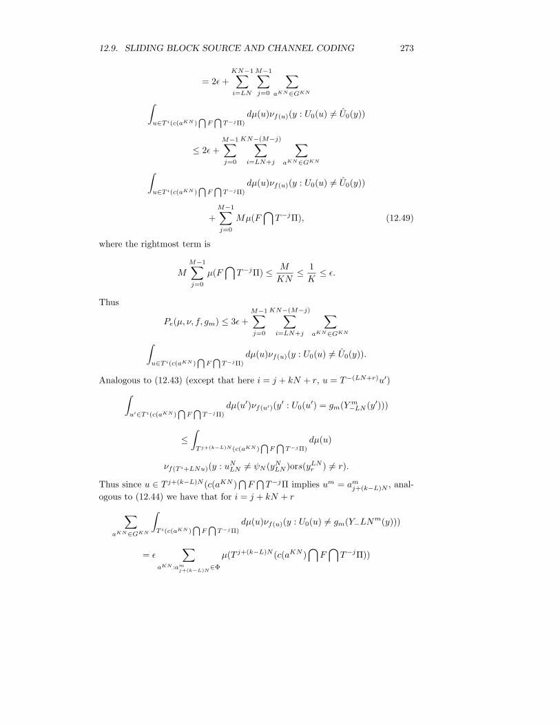
12.9. SLIDING BLOCK SOURCE AND CHANNEL CODING 273
= 2ε +KN−1∑i=LN
M−1∑j=0
∑aKN∈GKN∫
u∈T i(c(aKN )⋂
F⋂
T−jΠ)
dµ(u)νf(u)(y : U0(u) 6= U0(y))
≤ 2ε +M−1∑j=0
KN−(M−j)∑i=LN+j
∑aKN∈GKN∫
u∈T i(c(aKN )⋂
F⋂
T−jΠ)
dµ(u)νf(u)(y : U0(u) 6= U0(y))
+M−1∑j=0
Mµ(F⋂
T−jΠ), (12.49)
where the rightmost term is
MM−1∑j=0
µ(F⋂
T−jΠ) ≤ M
KN≤ 1
K≤ ε.
Thus
Pe(µ, ν, f, gm) ≤ 3ε +M−1∑j=0
KN−(M−j)∑i=LN+j
∑aKN∈GKN∫
u∈T i(c(aKN )⋂
F⋂
T−jΠ)
dµ(u)νf(u)(y : U0(u) 6= U0(y)).
Analogous to (12.43) (except that here i = j + kN + r, u = T−(LN+r)u′)∫u′∈T i(c(aKN )
⋂F
⋂T−jΠ)
dµ(u′)νf(u′)(y′ : U0(u′) = gm(Y m−LN (y′)))
≤∫
T j+(k−L)N (c(aKN )⋂
F⋂
T−jΠ)
dµ(u)
νf(T i+LNu)(y : uNLN 6= ψN (yN
LN )ors(yLNr ) 6= r).
Thus since u ∈ T j+(k−L)N (c(aKN )⋂
F⋂
T−jΠ implies um = amj+(k−L)N , anal-
ogous to (12.44) we have that for i = j + kN + r
∑aKN∈GKN
∫T i(c(aKN )
⋂F
⋂T−jΠ)
dµ(u)νf(u)(y : U0(u) 6= gm(Y−LNm(y)))
= ε∑
aKN :amj+(k−L)N
∈Φ
µ(T j+(k−L)N (c(aKN )⋂
F⋂
T−jΠ))
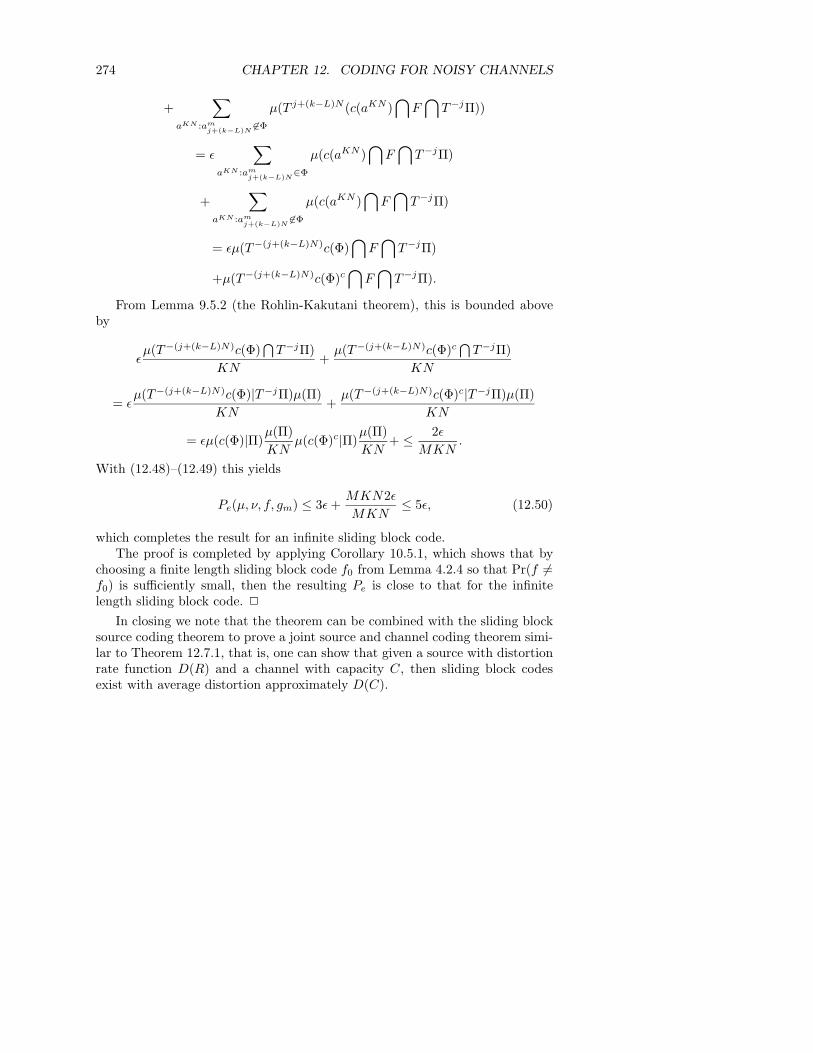
274 CHAPTER 12. CODING FOR NOISY CHANNELS
+∑
aKN :amj+(k−L)N
6∈Φ
µ(T j+(k−L)N (c(aKN )⋂
F⋂
T−jΠ))
= ε∑
aKN :amj+(k−L)N
∈Φ
µ(c(aKN )⋂
F⋂
T−jΠ)
+∑
aKN :amj+(k−L)N
6∈Φ
µ(c(aKN )⋂
F⋂
T−jΠ)
= εµ(T−(j+(k−L)N)c(Φ)⋂
F⋂
T−jΠ)
+µ(T−(j+(k−L)N)c(Φ)c⋂
F⋂
T−jΠ).
From Lemma 9.5.2 (the Rohlin-Kakutani theorem), this is bounded aboveby
εµ(T−(j+(k−L)N)c(Φ)
⋂T−jΠ)
KN+
µ(T−(j+(k−L)N)c(Φ)c⋂
T−jΠ)KN
= εµ(T−(j+(k−L)N)c(Φ)|T−jΠ)µ(Π)
KN+
µ(T−(j+(k−L)N)c(Φ)c|T−jΠ)µ(Π)KN
= εµ(c(Φ)|Π)µ(Π)KN
µ(c(Φ)c|Π)µ(Π)KN
+ ≤ 2ε
MKN.
With (12.48)–(12.49) this yields
Pe(µ, ν, f, gm) ≤ 3ε +MKN2ε
MKN≤ 5ε, (12.50)
which completes the result for an infinite sliding block code.The proof is completed by applying Corollary 10.5.1, which shows that by
choosing a finite length sliding block code f0 from Lemma 4.2.4 so that Pr(f 6=f0) is sufficiently small, then the resulting Pe is close to that for the infinitelength sliding block code. 2
In closing we note that the theorem can be combined with the sliding blocksource coding theorem to prove a joint source and channel coding theorem simi-lar to Theorem 12.7.1, that is, one can show that given a source with distortionrate function D(R) and a channel with capacity C, then sliding block codesexist with average distortion approximately D(C).
Bibliography
[1] N. M. Abramson. Information Theory and Coding. McGraw-Hill, NewYork, 1963.
[2] R. Adler. Ergodic and mixing properties of infinite memory channels.Proc. Amer. Math. Soc., 12:924–930, 1961.
[3] R. L. Adler, D. Coppersmith, and M. Hassner. Algorithms for sliding-block codes–an application of symbolic dynamics to information theory.IEEE Trans. Inform. Theory, IT-29:5–22, 1983.
[4] R. Ahlswede and P. Gacs. Two contributions to information theory. InTopics in Information Theory, pages 17–40, Keszthely,Hungary, 1975.
[5] R. Ahlswede and J. Wolfowitz. Channels without synchronization. Adv.in Appl. Probab., 3:383–403, 1971.
[6] P. Algoet. Log-Optimal Investment. PhD thesis, Stanford University, 1985.
[7] P. Algoet and T. Cover. A sandwich proof of the Shannon-McMillan-Breiman theorem. Ann. Probab., 16:899–909, 1988.
[8] E. Ayanoglu and R. M. Gray. The design of joint source and channel trelliswaveform coders. IEEE Trans. Inform. Theory, IT-33:855–865, November1987.
[9] A. R. Barron. The strong ergodic theorem for densities: generalizedShannon-McMillan-Breiman theorem. Ann. Probab., 13:1292–1303, 1985.
[10] T. Berger. Rate distortion theory for sources with abstract alphabets andmemory. Inform. and Control, 13:254–273, 1968.
[11] T. Berger. Rate Distortion Theory. Prentice-Hall Inc., EnglewoodCliffs,New Jersey, 1971.
[12] T. Berger. Multiterminal source coding. In G. Longo, editor, The In-formation Theory Approach to Communications, volume 229 of CISMCourses and Lectures, pages 171–231. Springer-Verlag, Vienna and NewYork, 1978.
275
276 BIBLIOGRAPHY
[13] E. Berlekamp. Algebraic Coding Theory. McGraw-Hill, New York, 1968.
[14] E. Berlekamp, editor. Key Papers in the Development of Coding Theory.IEEE Press, New York, 1974.
[15] P. Billingsley. Ergodic Theory and Information. Wiley, New York, 1965.
[16] G. D. Birkhoff. Proof of the ergodic theorem. Proc. Nat. Acad. Sci.,17:656–660, 1931.
[17] R. E. Blahut. Computation of channel capacity and rate-distortion func-tions. IEEE Trans. Inform. Theory, IT-18:460–473, 1972.
[18] R. E. Blahut. Theory and Practice of Error Control Codes. AddisonWesley, Reading, Mass., 1987.
[19] L. Breiman. The individual ergodic theorem of information theory. Ann.of Math. Statist., 28:809–811, 1957.
[20] L. Breiman. A correction to ‘The individual ergodic theorem of informa-tion theory’. Ann. of Math. Statist., 31:809–810, 1960.
[21] J. R. Brown. Ergodic Theory and Topological Dynamics. Academic Press,New York, 1976.
[22] J. A. Bucklew. A large deviation theory proof of the abstract alphabetsource coding theorem. IEEE Trans. Inform. Theory, IT-34:1081–1083,1988.
[23] T. M. Cover, P. Gacs, and R. M. Gray. Kolmogorov’s contributions toinformation theory and algorithmic complexity. Ann. Probab., 17:840–865,1989.
[24] I. Csiszar. Information-type measures of difference of probability distri-butions and indirect observations. Studia Scientiarum MathematicarumHungarica, 2:299–318, 1967.
[25] I. Csiszar. I-divergence geometry of probability distributions and mini-mization problems. Ann. Probab., 3(1):146–158, 1975.
[26] I. Csiszar and J. Korner. Coding Theorems of Information Theory. Aca-demic Press/Hungarian Academy of Sciences, Budapest, 1981.
[27] L. D. Davisson and R.M. Gray. A simplified proof of the sliding-blocksource coding theorem and its universal extension. In Conf. Record 1978Int’l. Conf. on Comm. 2, pages 34.4.1–34.4.5, Toronto, 1978.
[28] L. D. Davisson, R. J. McEliece, M. B. Pursley, and M. S. Wallace. Efficientuniversal noiseless source codes. IEEE Trans. Inform. Theory, IT-27:269–279, 1981.
BIBLIOGRAPHY 277
[29] L. D. Davisson and M. B. Pursley. An alternate proof of the coding the-orem for stationary ergodic sources. In Proceedings of the Eighth AnnualPrinceton Conference on Information Sciences and Systems, 1974.
[30] M. Denker, C. Grillenberger, and K. Sigmund. Ergodic Theory on CompactSpaces, volume 57 of Lecture Notes in Mathematics. Springer-Verlag, NewYork, 1970.
[31] J.-D. Deushcel and D. W. Stroock. Large Deviations, volume 137 of Pureand Applied Mathematics. Academic Press, Boston, 1989.
[32] R. L. Dobrushin. A general formulation of the fundamental Shannontheorem in information theory. Uspehi Mat. Akad. Nauk. SSSR, 14:3–104,1959. Translation in Transactions Amer. Math. Soc, series 2,vol. 33,323–438.
[33] R. L. Dobrushin. Shannon’s theorems for channels with synchronizationerrors. Problemy Peredaci Informatsii, 3:18–36, 1967. Translated in Prob-lems of Information Transmission, vol.,3,11–36 (1967),Plenum PublishingCorporation.
[34] M. D. Donsker and S. R. S. Varadhan. Asymptotic evaluation of certainMarkov process expectations for large time. J. Comm. Pure Appl. Math.,28:1–47, 1975.
[35] J. G. Dunham. A note on the abstract alphabet block source codingwith a fidelity criterion theorem. IEEE Trans. Inform. Theory, IT-24:760,November 1978.
[36] P. Elias. Two famous papers. IRE Transactions on Information Theory,page 99, 1958.
[37] R. M. Fano. Transmission of Information. Wiley, New York, 1961.
[38] A. Feinstein. A new basic theorem of information theory. IRE Transac-tions on Information Theory, pages 2–20, 1954.
[39] A. Feinstein. Foundations of Information Theory. McGraw-Hill, NewYork, 1958.
[40] A. Feinstein. On the coding theorem and its converse for finite-memorychannels. Inform. and Control, 2:25–44, 1959.
[41] G. D. Forney, Jr. The Viterbi algorithm. Proc. IEEE, 61:268–278, March1973.
[42] N. A. Friedman. Introduction to Ergodic Theory. Van Nostrand ReinholdCompany, New York, 1970.
[43] R. G. Gallager. Information Theory and Reliable Communication. JohnWiley & Sons, New York, 1968.
278 BIBLIOGRAPHY
[44] A. El Gamal and T. Cover. Multiple user information theory. Proc. IEEE,68:1466–1483, 1980.
[45] I. M. Gelfand, A. N. Kolmogorov, and A. M. Yaglom. On the generaldefinitions of the quantity of information. Dokl. Akad. Nauk, 111:745–748, 1956. (In Russian.).
[46] A. Gersho and V. Cuperman. Vector quantization: A pattern-matchingtechnique for speech coding. IEEE Communications Magazine, 21:15–21,December 1983.
[47] A. Gersho and R. M. Gray. Vector Quantization and Signal Compression.Kluwer Academic Publishers, Boston, 1992.
[48] R. M. Gray. Tree-searched block source codes. In Proceedings of the 1980Allerton Conference, Allerton IL, Oct. 1980.
[49] R. M. Gray. Vector quantization. IEEE ASSP Magazine, 1,No. 2:4–29,April 1984.
[50] R. M. Gray. Probability, Random Processes, and Ergodic Properties.Springer-Verlag, New York, 1988.
[51] R. M. Gray. Spectral analysis of quantization noise in a single-loop sigma-delta modulator with dc input. IEEE Trans. Comm., COM-37:588–599,1989.
[52] R. M. Gray. Source Coding Theory. Kluwer Academic Press, Boston,1990.
[53] R. M. Gray and L. D. Davisson. Source coding without the ergodic as-sumption. IEEE Trans. Inform. Theory, IT-20:502–516, 1974.
[54] R. M. Gray and J. C. Kieffer. Asymptotically mean stationary measures.Ann. Probab., 8:962–973, 1980.
[55] R. M. Gray, D. L. Neuhoff, and J. K. Omura. Process definitions of dis-tortion rate functions and source coding theorems. IEEE Trans. Inform.Theory, IT-21:524–532, 1975.
[56] R. M. Gray, D. L. Neuhoff, and D. Ornstein. Nonblock source coding witha fidelity criterion. Ann. Probab., 3:478–491, 1975.
[57] R. M. Gray, D. L. Neuhoff, and P. C. Shields. A generalization of ornstein’sd-bar distance with applications to information theory. Ann. Probab.,3:315–328, April 1975.
[58] R. M. Gray and D. S. Ornstein. Sliding-block joint source/noisy-channelcoding theorems. IEEE Trans. Inform. Theory, IT-22:682–690, 1976.
BIBLIOGRAPHY 279
[59] R. M. Gray, D. S. Ornstein, and R. L. Dobrushin. Blocksynchronization,sliding-block coding, invulnerable sources and zero errorcodes for discrete noisy channels. Ann. Probab., 8:639–674, 1980.
[60] R. M. Gray, M. Ostendorf, and R. Gobbi. Ergodicity of Markov channels.IEEE Trans. Inform. Theory, 33:656–664, September 1987.
[61] R. M. Gray and F. Saadat. Block source coding theory for asymptoticallymean stationary sources. IEEE Trans. Inform. Theory, 30:64–67, 1984.
[62] P. R. Halmos. Lectures on Ergodic Theory. Chelsea, New York, 1956.
[63] G. H. Hardy, J. E. Littlewood, and G. Polya. Inequalities. CambridgeUniv. Press, London, 1952. Second Edition,1959.
[64] R. V. L. Hartley. Transmission of information. Bell System Tech. J.,7:535–563, 1928.
[65] E. Hoph. Ergodentheorie. Springer-Verlag, Berlin, 1937.
[66] K. Jacobs. Die Ubertragung diskreter Informationen durch periodishceund fastperiodische Kanale. Math. Annalen, 137:125–135, 1959.
[67] K. Jacobs. Uber die Struktur der mittleren Entropie. Math. Z., 78:33–43,1962.
[68] K. Jacobs. The ergodic decomposition of the Kolmogorov-Sinai invariant.In F. B. Wright and F. B. Wright, editors, Ergodic Theory. AcademicPress, New York, 1963.
[69] N. S. Jayant and P. Noll. Digital Coding of Waveforms. Prentice-Hall,Englewood Cliffs,New Jersey, 1984.
[70] T. Kadota. Generalization of feinstein’s fundamental lemma. IEEE Trans.Inform. Theory, IT-16:791–792, 1970.
[71] S. Kakutani. Induced measure preserving transformations. In Proceedingsof the Imperial Academy of Tokyo, volume 19, pages 635–641, 1943.
[72] A. J. Khinchine. The entropy concept in probability theory. UspekhiMatematicheskikh Nauk., 8:3–20, 1953. Translated in Mathematical Foun-dations of Information Theory,Dover New York (1957).
[73] A. J. Khinchine. On the fundamental theorems of information theory.Uspekhi Matematicheskikh Nauk., 11:17–75, 1957. Translated in Mathe-matical Foundations of Information Theory,Dover New York (1957).
[74] J. C. Kieffer. A counterexample to Perez’s generalization of the Shannon-McMillan theorem. Ann. Probab., 1:362–364, 1973.
[75] J. C. Kieffer. A general formula for the capacity of stationary nonantici-patory channels. Inform. and Control, 26:381–391, 1974.
280 BIBLIOGRAPHY
[76] J. C. Kieffer. On the optimum average distortion attainable by fixed-ratecoding of a nonergodic source. IEEE Trans. Inform. Theory, IT-21:190–193, March 1975.
[77] J. C. Kieffer. A generalization of the pursley-davisson-mackenthun uni-versal variable-rate coding theorem. IEEE Trans. Inform. Theory, IT-23:694–697, 1977.
[78] J. C. Kieffer. A unified approach to weak universal source coding. IEEETrans. Inform. Theory, IT-24:674–682, 1978.
[79] J. C. Kieffer. Extension of source coding theorems for block codes tosliding block codes. IEEE Trans. Inform. Theory, IT-26:679–692, 1980.
[80] J. C. Kieffer. Block coding for weakly continuous channels. IEEE Trans.Inform. Theory, IT-27:721–727, 1981.
[81] J. C. Kieffer. Sliding-block coding for weakly continuous channels. IEEETrans. Inform. Theory, IT-28:2–10, 1982.
[82] J. C. Kieffer. Coding theorem with strong converse for block source codingsubject to a fidelity constraint, 1989. Preprint.
[83] J. C. Kieffer. An ergodic theorem for constrained sequences of functions.Bulletin American Math Society, 1989.
[84] J. C. Kieffer. Sample converses in source coding theory, 1989. Preprint.
[85] J. C. Kieffer. Elementary information theory. Unpublished manuscript,1990.
[86] J. C. Kieffer and M. Rahe. Markov channels are asymptotically meanstationary. Siam Journal of Mathematical Analysis, 12:293–305, 1980.
[87] A. N. Kolmogorov. On the Shannon theory of information in the caseof continuous signals. IRE Transactions Inform. Theory, IT-2:102–108,1956.
[88] A. N. Kolmogorov. A new metric invariant of transitive dynamic systemsand automorphisms in lebesgue spaces. Dokl. Akad. Nauk SSR, 119:861–864, 1958. (In Russian.).
[89] A. N. Kolmogorov. On the entropy per unit time as a metric invariantof automorphisms. Dokl. Akad. Naud SSSR, 124:768–771, 1959. (In Rus-sian.).
[90] A. N. Kolmogorov, A. M. Yaglom, and I. M. Gelfand. Quantity of in-formation and entropy for continuous distributions. In Proceedings 3rdAll-Union Mat. Conf., volume 3, pages 300–320. Izd. Akad. Nauk. SSSR,1956.
BIBLIOGRAPHY 281
[91] S. Kullback. A lower bound for discrimination in terms of variation. IEEETrans. Inform. Theory, IT-13:126–127, 1967.
[92] S. Kullback. Information Theory and Statistics. Dover, New York, 1968.Reprint of 1959 edition published by Wiley.
[93] B. M. Leiner and R. M. Gray. Bounds on rate-distortion functions forstationary sources and context-dependent fidelity criteria. IEEE Trans.Inform. Theory, IT-19:706–708, Sept. 1973.
[94] V. I. Levenshtein. Binary codes capable of correcting deletions, inser-tions,and reversals. Sov. Phys.-Dokl., 10:707–710, 1966.
[95] S. Lin. Introduction to Error Correcting Codes. Prentice-Hall, EnglewoodCliffs,NJ, 1970.
[96] K. M. Mackenthun and M. B. Pursley. Strongly and weakly universalsource coding. In Proceedings of the 1977 Conference on InformationScience and Systems, pages 286–291, Johns Hopkins University, 1977.
[97] F. J. MacWilliams and N. J. A. Sloane. The Theory of Error-CorrectingCodes. North-Holland, New York, 1977.
[98] A. Maitra. Integral representations of invariant measures. Transactionsof the American Mathematical Society, 228:209–235, 1977.
[99] J. Makhoul, S. Roucos, and H. Gish. Vector quantization in speech coding.Proc. IEEE, 73. No. 11:1551–1587, November 1985.
[100] B. Marcus. Sophic systems and encoding data. IEEE Trans. Inform.Theory, IT-31:366–377, 1985.
[101] K. Marton. On the rate distortion function of stationary sources. Problemsof Control and Information Theory, 4:289–297, 1975.
[102] R. McEliece. The Theory of Information and Coding. Cambridge Univer-sity Press, New York, NY, 1984.
[103] B. McMillan. The basic theorems of information theory. Ann. of Math.Statist., 24:196–219, 1953.
[104] L. D. Meshalkin. A case of isomorphisms of bernoulli scheme. Dokl. Akad.Nauk SSSR, 128:41–44, 1959. (In Russian.).
[105] Shu-Teh C. Moy. Generalizations of Shannon-McMillan theorem. PacificJournal Math., 11:705–714, 1961.
[106] J. Nedoma. On the ergodicity and r-ergodicity of stationary probabilitymeasures. Z. Wahrsch. Verw. Gebiete, 2:90–97, 1963.
282 BIBLIOGRAPHY
[107] J. Nedoma. The synchronization for ergodic channels. Transactions ThirdPrague Conf. Information Theory, Stat. Decision Functions,and RandomProcesses, pages 529–539, 1964.
[108] D. L. Neuhoff and R. K. Gilbert. Causal source codes. IEEE Trans.Inform. Theory, IT-28:701–713, 1982.
[109] D. L. Neuhoff, R. M. Gray, and L. D. Davisson. Fixed rate universalblock source coding with a fidelity criterion. IEEE Trans. Inform. Theory,21:511–523, 1975.
[110] D. L. Neuhoff and P. C. Shields. Channels with almost finite memory.IEEE Trans. Inform. Theory, pages 440–447, 1979.
[111] D. L. Neuhoff and P. C. Shields. Channel distances and exact representa-tion. Inform. and Control, 55(1), 1982.
[112] D. L. Neuhoff and P. C. Shields. Channel entropy and primitive approxi-mation. Ann. Probab., 10(1):188–198, 1982.
[113] D. L. Neuhoff and P. C. Shields. Indecomposable finite state channelsand primitive approximation. IEEE Trans. Inform. Theory, IT-28:11–19,1982.
[114] D. Ornstein. Bernoulli shifts with the same entropy are isomorphic. Ad-vances in Math., 4:337–352, 1970.
[115] D. Ornstein. An application of ergodic theory to probability theory. Ann.Probab., 1:43–58, 1973.
[116] D. Ornstein. Ergodic Theory,Randomness,and Dynamical Systems. YaleUniversity Press, New Haven, 1975.
[117] D. Ornstein and B. Weiss. The Shannon-McMillan-Breiman theorem fora class of amenable groups. Israel J. of Math, 44:53–60, 1983.
[118] D. O’Shaughnessy. Speech Communication. Addison-Wesley, Reading,Mass., 1987.
[119] P. Papantoni-Kazakos and R. M. Gray. Robustness of estimators on sta-tionary observations. Ann. Probab., 7:989–1002, Dec. 1979.
[120] A. Perez. Notions generalisees d’incertitude,d’entropie et d’information dupoint de vue de la theorie des martingales. In Transactions First PragueConf. on Information Theory, Stat. Decision Functions,and Random Pro-cesses, pages 183–208. Czech. Acad. Sci. Publishing House, 1957.
[121] A. Perez. Sur la convergence des incertitudes,entropies et informationsechantillon vers leurs valeurs vraies. In Transactions First Prague Conf.on Information Theory, Stat. Decision Functions,and Random Processes,pages 245–252. Czech. Acad. Sci. Publishing House, 1957.
BIBLIOGRAPHY 283
[122] A. Perez. Sur la theorie de l’information dans le cas d’un alphabet abstrait.In Transactions First Prague Conf. on Information Theory, Stat. DecisionFunctions,Random Processes, pages 209–244. Czech. Acad. Sci. PublishingHouse, 1957.
[123] A. Perez. Extensions of Shannon-McMillan’s limit theorem to more gen-eral stochastic processes processes. In Third Prague Conf. on Inform.Theory,Decision Functions,and Random Processes, pages 545–574, Pragueand New York, 1964. Publishing House Czech. Akad. Sci. and AcademicPress.
[124] K. Petersen. Ergodic Theory. Cambridge University Press, Cambridge,1983.
[125] M. S. Pinsker. Dynamical systems with completely positive or zero en-tropy. Soviet Math. Dokl., 1:937–938, 1960.
[126] D. Ramachandran. Perfect Measures. ISI Lecture Notes,No. 6 and 7.Indian Statistical Institute, Calcutta,India, 1979.
[127] V. A. Rohlin and Ya. G. Sinai. Construction and properties of invariantmeasurable partitions. Soviet Math. Dokl., 2:1611–1614, 1962.
[128] V. V. Sazanov. On perfect measures. Izv. Akad. Nauk SSSR, 26:391–414,1962. American Math. Soc. Translations,Series 2, No. 48,pp. 229-254,1965.
[129] C. E. Shannon. A mathematical theory of communication. Bell Syst.Tech. J., 27:379–423,623–656, 1948.
[130] C. E. Shannon. Coding theorems for a discrete source with a fidelitycriterion. In IRE National Convention Record,Part 4, pages 142–163,1959.
[131] P. C. Shields. The Theory of Bernoulli Shifts. The University of ChicagoPress, Chicago,Ill., 1973.
[132] P. C. Shields. The ergodic and entropy theorems revisited. IEEE Trans.Inform. Theory, IT-33:263–266, 1987.
[133] P. C. Shields and D. L. Neuhoff. Block and sliding-block source coding.IEEE Trans. Inform. Theory, IT-23:211–215, 1977.
[134] Ya. G. Sinai. On the concept of entropy of a dynamical system. Dokl.Akad. Nauk. SSSR, 124:768–771, 1959. (In Russian.).
[135] Ya. G. Sinai. Weak isomorphism of transformations with an invariantmeasure. Soviet Math. Dokl., 3:1725–1729, 1962.
[136] Ya. G. Sinai. Introduction to Ergodic Theory. MathematicalNotes,Princeton University Press, Princeton, 1976.
284 BIBLIOGRAPHY
[137] D. Slepian. A class of binary signaling alphabets. Bell Syst. Tech. J.,35:203–234, 1956.
[138] D. Slepian, editor. Key Papers in the Development of Information Theory.IEEE Press, New York, 1973.
[139] A. D. Sokai. Existence of compatible families of proper regular conditionalprobabilities. Z. Wahrsch. Verw. Gebiete, 56:537–548, 1981.
[140] J. Storer. Data Compression. Computer Science Press, Rockville, Mary-land, 1988.
[141] I. Vajda. A synchronization method for totally ergodic channels. In Trans-actions of the Fourth Prague Conf. on Information Theory,Decision Func-tions,and Random Processes, pages 611–625, Prague, 1965.
[142] E. van der Meulen. A survey of multi-way channels in information theory:1961–1976. IEEE Trans. Inform. Theory, IT-23:1–37, 1977.
[143] S. R. S. Varadhan. Large Deviations and Applications. Society for Indus-trial and Applied Mathematics, Philadelphia, 1984.
[144] L. N. Vasershtein. Markov processes on countable product space describinglarge systems of automata. Problemy Peredachi Informatsii, 5:64–73, 1969.
[145] A. J. Viterbi and J. K. Omura. Principles of Digital Communication andCoding. McGraw-Hill, New York, 1979.
[146] J. von Neumann. Zur operatorenmethode in der klassischen mechanik.Ann. of Math., 33:587–642, 1932.
[147] P. Walters. Ergodic Theory-Introductory Lectures. Lecture Notes in Math-ematics No. 458. Springer-Verlag, New York, 1975.
[148] E. J. Weldon, Jr. and W. W. Peterson. Error Correcting Codes. MITPress, Cambridge, Mass., 1971. Second Ed.
[149] K. Winkelbauer. Communication channels with finite past history. Trans-actions of the Second Prague Conf. on Information Theory,Decision Func-tions,and Random Processes, pages 685–831, 1960.
[150] J. Wolfowitz. Strong converse of the coding theorem for the general dis-crete finite-memory channel. Inform. and Control, 3:89–93, 1960.
[151] J. Wolfowitz. Coding Theorems of Information Theory. Springer-Verlag,New York, 1978. Third edition.
[152] A. Wyner. A definition of conditional mutual information for arbitraryensembles. Inform. and Control, pages 51–59, 1978.