Journal of Hydrology 442–443 (2012) 105–116

Contents lists available at SciVerse ScienceDirect

Journal of Hydrology

journal homepage: www.elsevier .com/ locate / jhydrol

Ensemble Streamflow Prediction: Climate signal weighting methodsvs. Climate Forecast System Reanalysis

Mohammad Reza Najafi a, Hamid Moradkhani a,⇑, Thomas C. Piechota b

a Department of Civil and Environmental Engineering, Portland State University, Portland, Oregon, United Statesb Department of Civil and Environmental Engineering, University of Nevada, Las Vegas, Nevada, United States

a r t i c l e i n f o s u m m a r y

Article history:Received 16 August 2011Received in revised form 23 March 2012Accepted 1 April 2012Available online 7 April 2012This manuscript was handled byKonstantine P. Georgakakos, Editor-in-Chief,with the assistance of Attilio Castellarin,Associate Editor

Keywords:Ensemble Streamflow PredictionClimate signalPCACFSRPost-processing

0022-1694/$ - see front matter � 2012 Elsevier B.V. Ahttp://dx.doi.org/10.1016/j.jhydrol.2012.04.003

⇑ Corresponding author. Tel.: +1 503 725 2436.E-mail address: hamidm@cecs.pdx.edu (H. Moradk

Ensemble Streamflow Prediction (ESP) provides the means for statistical post-processing of forecasts andestimating the inherent uncertainties. In addition, large scale climate variables provide valuable informa-tion for hydrologic predictions. In this study we develop methods to assign weights to ESP ensemblemembers according to climate signals which are selected based on the spearman’s rank correlation coeffi-cients. Analysis was performed over the snow dominated East River basin to improve the spring streamflowvolumetric forecast. Principle Component Analysis (PCA) was found to increase the accuracy of the weight-ing scheme considerably. We compare five parametric and nonparametric weighting methods includingFuzzy C-Means clustering, Formal Likelihood, Informal Likelihood and two variants of K-Nearest Neighborsapproaches. The methods are found to be simple and efficient while the results seem promising. The pre-dictions, based on simple average or the median of the ensemble members, combined with the weightedensemble forecasts provide improved estimates of probable streamflow ranges and the uncertainty bounds.Improvement in the weighting approach was obtained by selecting the climate signals, choosing the rightnumber of principle components and considering several weighting approaches. As an alternative approachto ESP, an additional climate dataset, the Climate Forecast System Reanalysis (CFSR) provided via theNational Centers for Environmental Prediction (NCEP) in its most recent reanalysis project was tested.

� 2012 Elsevier B.V. All rights reserved.

1. Introduction

Currently the two major approaches for streamflow forecastinginclude the statistical methods (i.e. linear regression), and theEnsemble Streamflow Prediction (ESP) (Moradkhani and Meier,2010). Although ESP utilizes sophisticated models and requiresadditional data analysis compared to the regression based models,it provides flexibility that further enhances the predictions byincorporating basin’s initial condition and meteorological informa-tion. ESP, previously named extended streamflow forecast, was firstintroduced by the National Weather Service (NWS) (Day, 1985) andhas since gained much attention. It is currently implemented in theNWS Advance Hydrologic Prediction Service (AHPS) (McEnery et al.,2005). The National Weather service (NWS) with various opera-tional responsibilities (Larson et al., 1995) through its network ofRiver Forecast Centers along with the Natural Resources Conserva-tion Service (NRCS), provide streamflow forecasts to the users in theUnited States (Twedt et al., 1977). The NWS issues volumetric watersupply forecasts of naturalized flows ranging from January 1st up tothe end of the snow accumulation season.

ll rights reserved.

hani).

In ESP, the calibrated hydrologic model is run, prior to forecasttime, until the watershed’s initial conditions are reflected. Themodel is then driven by resampled historical meteorological data,meteorological forecasts or climate outlooks to generate an ensem-ble of possible future streamflow in the basin (Fig. 1). The ESP proce-dure is based on the assumption that the historical meteorologicalevents are representative of events that may occur in the future. Inother words, each historical data is treated as a realization of theatmospheric forcing which is used to simulate the streamflowtraces. This grants ESP the basis for considering the uncertainty per-tained to the future climate, which may be the major component offorecast uncertainty in some seasons (Wood and Lettenmaier, 2008).In operational settings, such as NWS, the ESP is issued for short term(0–10 days), midterm (0–120 days) and long term (0–365 days)hydrologic forecasting. Statistical averaging can then be applied inorder to issue deterministic forecasts. Considering the seasonal fore-cast, the mean or median of the ensemble runoff volume is com-monly reported as the single (possibly best) prediction. Ensembleforecasting provides the means for statistical post-processing inaddition to an estimate of the inherent forecast uncertainty. Onepopular post-processing method is to bias-correct the forecastensembles using quantile mapping (QM) technique (Leung et al.,1999). With this method, a mapping between observation and sim-ulation cumulative distribution functions (CDFs) is implemented

... ...Resampled Historical Precipitation

Trajectories of Streamflow

Hydrological Model

State Initial condition

StatisticalAnalysis

Fig. 1. ESP schematic view.

106 M.R. Najafi et al. / Journal of Hydrology 442–443 (2012) 105–116

and the forecast ensemble mean is bias corrected. A major drawbackof this method, however, is that it does not maintain the pairing ofcorresponding simulated and observed flows. To overcome thelimitation of QM method, Madadgar et al. (2012) proposed a newpost-processing method by applying a group of multivariate proba-bility functions, the so-called copula functions, Using copulafunctions, the conditional probability of the observed variable canbe estimated at any particular forecast value (Madadgar andMoradkhani, in press).

ESP traces which reflect the contribution of resampled meteoro-logical data in streamflow forecasts are considered neither the truerepresentatives of the future observable variables nor the probabi-listic forecasts of future runoffs. Instead, they can be utilized toinfer the runoff probability (Stephenson et al., 2005). The lack ofknowledge about future meteorological conditions, especially ex-treme events, would influence the resulting ensemble predictions.A further compounding factor is that including weather predictionsmay or may not improve the current short term ESP forecasts (lessthan 14 days) let alone their capability to provide accurate mid/long lead forecasts. On the other hand, ESP considers the inputuncertainties (i.e. precipitation and temperature) and ignores theuncertainties in the initial condition (DeChant and Moradkhani,2011b; Wood and Schaake, 2008). However, model prediction issubject to other uncertainties and sources of forecast errors.Uncertainties may stem from model initialization because ofincomplete data coverage, observation errors, and imperfectionsof the model structure itself, mainly due to parameterization andspatiotemporal discretization of physical processes (Moradkhaniand Sorooshian, 2008; Parrish et al., 2012).

Further improvement of probabilistic streamflow forecast accu-racy can be achieved by including information from meteorologicalforecasts and climate outlooks in the ESP approach, particularly forthe short term predictions. Recent studies have assessed the appli-cation of short/medium-range numerical weather prediction mod-el output to short-term streamflow forecasting with the intentionof further reducing ensemble spread (Clark and Hay, 2004; Thirelet al., 2008). They replaced the meteorological inputs, resampledfrom the historical series, with the atmospheric model results.Their study emphasized that the systematic biases which exist inweather prediction models should be removed before any hydro-logical analysis. Wood et al. (2005) compared ESP results vs.streamflow forecasts obtained from the climate models for theWestern United States and found that during ENSO conditionsthe Global Spectral Model (GSM) forecast may or may not enhancethe hydrologic forecasts relative to ESP for each study area and sea-son. The impact of initial state uncertainty in ensemble streamflowforecasting is analyzed in various studies. Wood and Lettenmaier(2008) proposed the approach of Reverse-ESP to consider the im-pact of uncertain initial conditions (ICs). Their results indicatedthat the relative importance of IC and climate data depends onthe time of prediction, lead time, and location under study. Liet al. (2009) found that the initial condition uncertainty is domi-nant in forecasts with lead time of 1 month. Given the problemsassociated with averaging the ensemble members, Seo et al.

(2006) proposed an autoregressive-1 model, to enhance the meanof the ensemble traces for a short lead time Ensemble StreamflowPrediction.

It is well-recognized that climate information plays a significantrole in seasonal runoff forecasting (Moradkhani and Meier, 2010;Smith, 1992). Interannual precipitation variability is the mainsource of atmospheric forcing errors which impacts the streamflowprediction considerably (Li et al., 2009). Large scale climate signalsprovide valuable information about the meteorological variabilityand can be used to improve mid/long term predictions. Climatesignals have been incorporated as predictors in several studies toimprove the statistical streamflow volume prediction (Kennedyet al., 2009; Moradkhani and Meier, 2010; Regonda et al., 2006).For the Colorado River basin, Timilsena et al. (2009) found a largermagnitude of streamflow changes in the lower basin comparedwith the upper basin as an influence of the climate signals. Theirresults showed an increase in streamflow during El Nino and warmphase of PDO and vice versa. Grantz et al. (2005) used an ensembleprediction method for streamflow forecasting over the westernUnited States and showed that large-scale climate informationcan be incorporated as predictors for spring streamflow forecastwith a lead time up to 4 months, starting from December. Histori-cal climatologic data bootstrapping for ESP forcing were recentlyconditioned on the teleconnection similarity, especially ENSO andPDO, between the previous years and the forecast year (Woodand Lettenmaier, 2006). Studies show improved results comparedto the unconditional ESP approach. Hamlet and Lettenmaier(1999) found an increase in forecast lead time and specificity overclimatology by restricting the ensemble members to years that aresimilar in terms of El Nino-Southern Oscillation (ENSO) and PacificDecadal Oscillation (PDO) phases. The approach lead to a set ofensemble members that exhibited tighter clustering compared tothe full ensemble.

In spite of these recent advancements there is still the need toincorporate climate signals as a weighting scheme in ESP post-processing. Current techniques, as applied in Hamlet andLettenmaier (1999) and Werner et al. (2004), provide insight intothe benefit of climate signals in ESP weighting, however, furtherinvestigation is required. The method proposed by Hamlet andLettenmaier (1999) ignores information in ensemble members thatare not in ENSO (PDO) categories throughout the forecast year. Themethod presented by Werner et al. (2004) considers the average ofclimate indices to provide a vector predictor but they do notprovide details on how to rely on parameters selected within themethod. However they do provide the following useful conclu-sions: (1) the importance of weighting the ensemble membersand considering all traces instead of discarding some, and (2) thehigher performance of the ESP post-processing comparing to thepre-processing given the weighting procedure.

This study provides a more comprehensive analysis of possibleimprovements to seasonal forecasts using the climate signalthrough a post-processing weighting approach. ESP traces areweighted using similarity assessment methods applied on the cli-mate signals. A dimension reduction technique is considered to re-move the redundancy in the data allowing for incorporatingvarious indices in the weighting process. Furthermore, climateforecast data from the National Centers for Environmental Predic-tion (NCEP) most recent reanalysis project, the so called ClimateForecast System Reanalysis (CFSR) (Saha et al., 2010), was usedas input to the hydrologic model. A recent study by Ebisuzakiand Zhang (2011) has shown improved climate forecast as com-pared to the previous CFS datasets while the new forecast providesthe finer resolution data sets. We compare and contrast the hydro-logic forecast based on this new dataset with the conventional ESPas well as the results obtained from the weighting procedure.

M.R. Najafi et al. / Journal of Hydrology 442–443 (2012) 105–116 107

2. Study area and data

The snow dominated East River basin is a tributary of the Gunn-ison River in the Colorado River basin (see Fig. 2) (DeChant andMoradkhani, 2011a). The river basin is 754 km2 with the elevationranging from 2445 m to 3898 m. The Gunnison River is the fifthlargest tributary of the Colorado River basin (CRB), therefore esti-mation of the water volume stored in snow, and its impact onstreamflow in upper tributaries, is important for water supply fore-casting in CRB (DeChant and Moradkhani, 2011a). For the East riverbasin, the primary data used in this study was obtained from theNWS CBRFC and consists of six-hourly precipitation and tempera-ture data for each of the three elevation zones along with dailystreamflow in the outlet. The duration of the streamflow data is1975–2005 and the forcing data 1960–2005. One of the advantagesof ESP is that the model is capable of running with all the historicalmeteorological data available, even though the streamflowmeasurements may not cover the whole period. Eighteen climateindices are considered in this study, as summarized in Table 1.

For comparison purposes, climate forecast model informationfrom NCAR’s CFSR project is used as an alternative approach toESP for providing streamflow predictions. The CFSR dataset pro-vides an extensive collection of climate variable information. In

Fig. 2. East Ri

this study six hourly averages of hourly temperature and precipita-tion data at a spatial resolution of approximately 38 km (Sahaet al., 2010) was obtained from the Computational and Informa-tional Systems Laboratory (CISL) Research Data Archive (http://dss.ucar.edu/pub/cfsr.html). The CFSR dataset provides detailedclimate information using the most up to date data assimilationtechniques as well as highly advanced (and coupled) atmospheric,oceanic, and surface modeling components. Details related to theCFSR data assimilation methods, modeling components andcoupling approaches are available in (Saha et al., 2010).

3. Methodology

The NWSRFS combines the SNOW-17 model with the Sacra-mento Soil Moisture Accounting Model (SAC-SMA) in order to pre-dict streamflow (Laurine et al., 1996) in snow dominated basins.Using these two models we first perform the ESP. The ensemblemean is then considered as the simulated volumetric streamflow.Next a procedure to weight the ensemble traces based on theclimate signals is proposed. The CFSR version 2 as forcing data tothe hydrologic models is evaluated in a deterministic as well asprobabilistic (i.e. ESP) conditions.

ver basin.

Table 1Climate indices that are correlated with the spring runoff in order to defineweights for ensemble streamflow generation. Source: http://www.esrl.noaa.gov/data/climateindices/list/

Climate signal Abbreviation

Northern Oscillation Index NOINino1 + 2 Nino 12Nino 3 Index Nino 3Nino 3.4 Nino 34Nino 4 Index Nino 4Pacific–North American pattern NAONorth Pacific pattern� NPEast Pacific/North Pacific Oscillation EPOMultivariate ENSO Index MEIBivariate Enso time-series BETWest Pacific pattern WPPacific Decadal Oscillation PDOSouthern Oscillation Index SOIPacific North American Index PNANorth Tropical Atlantic Index NTAOcean Nino Index ONIPacific EOF EOFPACPacific Warmpool PACWARM

1980 1985 1990 1995 2000 20050

20

40

60

80

100

120

140

Time

Stre

amflo

w (C

MS) NSE = 0.74

ObservationSimulation

Fig. 3. Observed vs. simulated runoff in the East river basin.

108 M.R. Najafi et al. / Journal of Hydrology 442–443 (2012) 105–116

3.1. Models

SNOW-17 is a lumped model that simulates the snow processesover a vertical column by employing a temperature-index energybalance approach (Anderson, 1973). It includes fourteen state vari-ables and twelve parameters. The model first determines the formof precipitation by either comparing the air temperature to a userdefined threshold temperature or other criteria as specified in(Anderson, 2002). It then estimates the depth and density of newsnow, based on the fraction of precipitation falling as snow andthe assumed precipitation gage catch deficiency.

The Sacramento Soil Moisture Accounting (SAC-SMA) model is alumped conceptual catchment water balance model developed byBurnash et al. (1973). The original version of the model has sixteenparameters (13 user-specifiable and three fixed) which define theconceptual linkage between the soil and water and an evapotrans-piration demand curve. The inputs to the model are mean arealprecipitation (MAP) and potential evapotranspiration (PET);streamflow at the channel is the output. The model consists ofsix state variables that represent the soil water content of theupper and lower soil zones in the form of free and tension water(Burnash, 1995). The soil moisture storages in both zones varydue to the non-linear dynamics of precipitation, percolation, evap-oration and lateral drainage.

In order to perform the hydrologic modeling over the East riverbasin, the temperature and precipitation were input to Snow-17 asforcing data to predict Snow Water Equivalent (SWE) in mm, SnowCover Area (SCA) as a fraction, and Rain plus Melt (RM) in mm ateach time step. The SAC-SMA was then driven by Rain plus Meltwhile Potential Evapotranspiration (PET) was also considered toestimate runoff.

3.2. ESP weighting procedures

The following sections elaborate on the procedure for generat-ing ensemble streamflows and the weighting approach based onclimate signals.

3.2.1. Model setupRainfall-runoff modeling of the East River basin was performed

based on calibrated parameters, the unit hydrograph, and PET ob-tained from the NWS CBRFC (NWSRFS, 2005). Monthly PET values,calculated from pan evaporation measurements (Farnsworth et al.,

1982), were disaggregated to daily values by linear interpolation.NWS categorizes the basin into three elevation zones, the upper,middle and lower zones. Due to lower temperatures in the upperzones there is commonly a time lag between the onset of snowmeltcompared to the middle and lower zones which should be consid-ered in the unit hydrograph parameterization. Separate parametersand unit hydrograph vectors were defined and adjusted manuallyfor each zone. Modeling was then performed independently foreach zone and the resulting cumulative runoff was compared withstreamflow measurements. Fig. 3 shows the performance of themodel for the period of analysis. A Nash–Sutcliff Efficiency (NSE)of 0.74 for the whole dataset was calculated.

3.2.2. Ensemble Streamflow PredictionForcing data ranging from 1961 up to the forecast year was con-

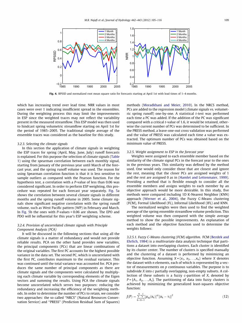
sidered when generating the ESP. The spin-up involved running themodels with the calibrated parameters for the same time period inorder to obtain the initial condition in the forecast year. The start-ing date of the ESP was April 1st in order to forecast runoff volumefor April–July. In order to evaluate the models we initially per-formed the analysis for the period of 1985–2005 over four leadtimes (1–4 months) all starting on April 1st. The two performancemeasures included the Ranked Probability Skill Score (RPSS) whichis widely used in probabilistic forecast verification (Wilks, 2006) isa measure of the closeness of the cumulative probabilities of theforecast and the observation. RPSS expresses the improvement ofthe ensemble forecast relative to the climatology in predictingthe category in which the observations lies. In this study, however,we applied the Debiased RPSS (i.e. RPSSD which is described inAppendix A) proposed by Weigel et al. (2007) as it removes thenegative bias in RPSS for small ensemble sizes.

The Normalized Root mean square Ratio (NRR) is used to measureensemble dispersion, indicating how confidently the ensemblemean could be extracted from ensemble spread (Leisenring andMoradkhani, 2011; Moradkhani and Meskele, 2009; Saha et al.,2010). NRR > 1 indicates that the ensemble has too little spread rel-ative to the predicted mean while NRR < 1 shows too much spread.

NRR ¼

ffiffiffiffiffiffiffiffiffiffiffiffiffiffiffiffiffiffiffiffiffiffiffiffiffiffiffiffiffiffiffiffiffiffiffiffiffiffi1

Nd

PNdt¼1ðyst � ytÞ

2q

1Ne

PNei¼1

ffiffiffiffiffiffiffiffiffiffiffiffiffiffiffiffiffiffiffiffiffiffiffiffiffiffiffiffiffiffiffiffiffiffiffiffiffiffiffiffiffiffi1

Nd

PNdt¼1ðysi

t � ytÞ2

h ir� � ffiffiffiffiffiffiffiffiNeþ12Ne

q ð11Þ

The period from 1975 up to the forecast year was used whencomparing the generated streamflow traces with the observedstreamflow. The performance of the generated ESPs for 3 leadtimes of 1–4 months was evaluated for 1985–2005 (Fig. 4). AnRPSSD score of 1 implies perfect probability forecast skillcompared with climatology. Overall RPSSD values are acceptable

1985 1990 1995 2000 2005−0.2

0

0.2

0.4

0.6

0.8

1

RPS

SD

1 Month2 Months3 Months4 Months

1985 1990 1995 2000 20050.2

0.4

0.6

0.8

1

1.2

1.4

1.6

1.8

NR

R

1 Month2 Months3 Months4 Months

Fig. 4. RPSSD and normalized root mean square ratio for forecasts starting at April 1st with lead times of 1–4 months.

M.R. Najafi et al. / Journal of Hydrology 442–443 (2012) 105–116 109

which has increasing trend over lead time. NRR values in mostcases were over 1 indicating insufficient spread in the ensembles.During the weighting process this may limit the improvementsin ESP since the weighted traces may not reflect the variabilitypresent in the measured streamflow. This ESP model was then usedto hindcast spring volumetric streamflow starting on April 1st forthe period of 1985–2005. The traditional simple average of theensemble traces was considered as the baseline for this study.

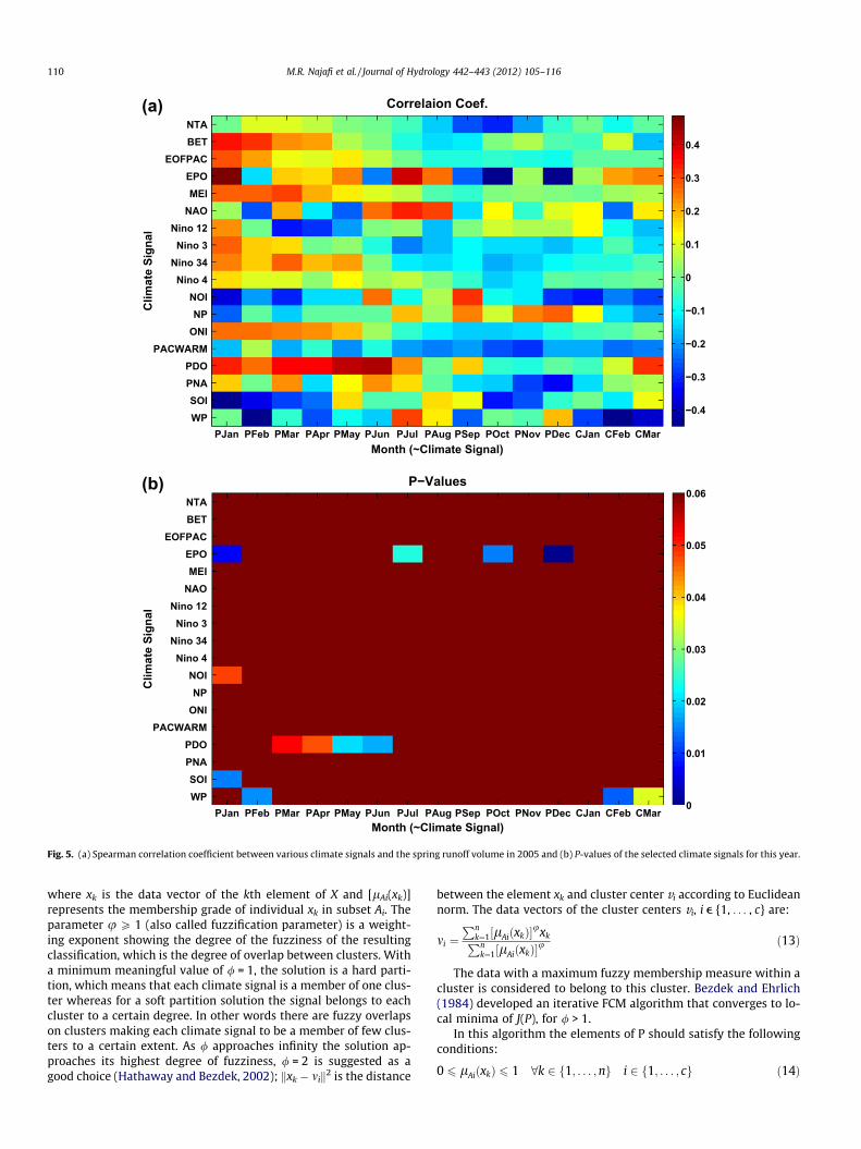
3.2.3. Selecting the climate signalsIn this section the application of climate signals in weighting

the ESP traces for spring (April, May, June, July) runoff forecastsis explained. For this purpose the selection of climate signals (Table1) using the spearman correlation between each monthly signal,starting from January of the previous year until March of the fore-cast year, and the spring runoff volume was used. The reason forusing Spearman correlation function is that it is less sensitive tosample outliers as compared with the Pearson function. For thehypothesis test, a correlation with a P-value of less than 0.06 wasconsidered significant. In order to perform ESP weighting, this pro-cedure was repeated for each forecast year separately. Fig. 5ashows the correlation between several climate signals in differentmonths and the spring runoff volume in 2005. Some climate sig-nals show significant negative correlation with the spring runoffvolume, such as West Pacific pattern (WP) in February and March.In Fig. 5b the ones with P-values < 0.06 are shown. The EPO andPDO will be influential for this year’s ESP weighting scheme.

3.2.4. Provision of uncorrelated climate signals with PrincipleComponent Analysis (PCA)

It will be discussed in the following sections that using all theclimate signals is a matter of redundancy and would not providereliable results. PCA on the other hand provides new variables,the principal components (PCs) that are linear combinations ofthe original variables. The first PC accounts for the highest possiblevariance in the data set. The second PC, which is uncorrelated withthe first PC, contributes maximum to the residual variance. Thiswas continued until the total variance was accounted for. PCA pro-duces the same number of principal components as there areclimate signals and the components were calculated by multiply-ing each climate variable by corresponding elements of the Eigenvectors and summing the results. Using PCA the climate signalsbecome uncorrelated which serves two purposes: reducing theredundancy and increasing the efficiency of the weighting meth-ods. In order to determine the number of PCs to retain, we considertwo approaches: the so called ‘‘NRCS’’ (Natural Resources Conser-vation Service) and ‘‘PRESS’’ (Prediction Residual Sum of Squares)

methods (Moradkhani and Meier, 2010). In the NRCS method,PCs are added to the regression model (climate signals vs. volumet-ric spring runoff) one-by-one. A statistical t-test was performedeach time a PC was added. If the addition of the PC was significantcompared with a critical t-value of 1.6, it would be retained, other-wise the current number of PCs was determined to be sufficient. Inthe PRESS method, a leave-one-out cross validation was performedand the value of PRESS was calculated each time a value was ex-tracted. The optimum number of PCs was obtained based on theminimum value of PRESS.

3.2.5. Weight assignment to ESP in the forecast yearWeights were assigned to each ensemble member based on the

similarity of the climate signal PCs in the forecast year to the onesin the previous years. This similarity was defined by the methodused. One would only consider those that are closest and ignorethe rest, meaning that the closer PCs are assigned weights of 1and the rest are assigned 0 as in (Hamlet and Lettenmaier, 1999).Providing a method that is flexible enough to consider all theensemble members and assigns weights to each member by anobjective approach would be more desirable. In this study, fivemethods were compared including 1D K-Nearest Neighbor (KNN)approach (Werner et al., 2004), the Fuzzy C-Means clustering(FCM), Formal Likelihood (FL), Informal Likelihood (IFL) and KNN.

The normalized weights were then used to find the weightedaverage of the spring ensemble streamflow volume prediction. Thisweighted volume was then compared with the simple averagemethod to show the possible improvements. An explanation ofeach method and the objective function used to determine theweights follows:

3.2.5.1. Fuzzy C-Means clustering (FCM) algorithm. FCM (Bezdek andEhrlich, 1984) is a multivariate data analysis technique that parti-tions a dataset into overlapping clusters. Each cluster is identifiedby its cluster center. The number of clusters is specified manuallyand the clustering of a dataset is performed by minimizing anobjective function. Assuming X = (x1, x2, . . . , xn) where X denotesthe dataset with n elements, each of which is represented by a vec-tor of measurements on p continuous variables. The purpose is tosubdivide X into c partially overlapping, non-empty subsets. A col-lection of these subsets is a fuzzy c-partition of X, denoted byP = {A1, A2, . . . ,Ac}. The partitioning of data into fuzzy clusters isachieved by minimizing the generalized least-squares objectivefunction:

JðPÞ ¼Pnk¼1

Pci¼1½lAiðxkÞ�ukxk � mik2 ð12Þ

Month (~Climate Signal)

Clim

ate

Sign

al

Correlaion Coef.

PJan PFeb PMar PApr PMay PJun PJul PAug PSep POct PNov PDec CJan CFeb CMar

NTABET

EOFPACEPOMEI

NAONino 12Nino 3

Nino 34Nino 4

NOINP

ONIPACWARM

PDOPNASOIWP

−0.4

−0.3

−0.2

−0.1

0

0.1

0.2

0.3

0.4

Month (~Climate Signal)

Clim

ate

Sign

al

P−Values

PJan PFeb PMar PApr PMay PJun PJul PAug PSep POct PNov PDec CJan CFeb CMar

NTABET

EOFPACEPOMEI

NAONino 12Nino 3

Nino 34Nino 4

NOINP

ONIPACWARM

PDOPNASOIWP

0

0.01

0.02

0.03

0.04

0.05

0.06

(a)

(b)

Fig. 5. (a) Spearman correlation coefficient between various climate signals and the spring runoff volume in 2005 and (b) P-values of the selected climate signals for this year.

110 M.R. Najafi et al. / Journal of Hydrology 442–443 (2012) 105–116

where xk is the data vector of the kth element of X and [lAi(xk)]represents the membership grade of individual xk in subset Ai. Theparameter u P 1 (also called fuzzification parameter) is a weight-ing exponent showing the degree of the fuzziness of the resultingclassification, which is the degree of overlap between clusters. Witha minimum meaningful value of / = 1, the solution is a hard parti-tion, which means that each climate signal is a member of one clus-ter whereas for a soft partition solution the signal belongs to eachcluster to a certain degree. In other words there are fuzzy overlapson clusters making each climate signal to be a member of few clus-ters to a certain extent. As / approaches infinity the solution ap-proaches its highest degree of fuzziness, / = 2 is suggested as agood choice (Hathaway and Bezdek, 2002); kxk � mik2 is the distance

between the element xk and cluster center vi according to Euclideannorm. The data vectors of the cluster centers vi, i e {1, . . . , c} are:

mi ¼Pn

k¼1½lAiðxkÞ�uxkPnk¼1½lAiðxkÞ�u

ð13Þ

The data with a maximum fuzzy membership measure within acluster is considered to belong to this cluster. Bezdek and Ehrlich(1984) developed an iterative FCM algorithm that converges to lo-cal minima of J(P), for / > 1.

In this algorithm the elements of P should satisfy the followingconditions:

0 6 lAiðxkÞ 6 1 8k 2 f1; . . . ;ng i 2 f1; . . . ; cg ð14Þ

0

10

20

30

40

Apr1−10Apr20−30

May11−20Jun1−10

Jun20−30Jul11−20

V 10 (k

af)

Yr:2000Obs.CFSRClimat. Avg.

0

10

20

30

40

Apr1−10Apr20−30

May11−20Jun1−10

Jun20−30Jul11−20

Yr:2001Obs.CFSRClimat. Avg.

0

5

10

15

20

Apr1−10Apr20−30

May11−20Jun1−10

Jun20−30Jul11−20

V 10 (k

af)

Yr:2002

0

10

20

30

40

Apr1−10Apr20−30

May11−20Jun1−10

Jun20−30Jul11−20

Yr:2003

0

10

20

30

40

Apr1−10Apr20−30

May11−20Jun1−10

Jun20−30Jul11−20

Period of Hindcast

V 10 (k

af)

Yr:2004

0

10

20

30

40

50

Apr1−10Apr20−30

May11−20Jun1−10

Jun20−30Jul11−20

Period of Hindcast

Yr:2005

Fig. 6. Comparison of total 10-day observed runoff volume vs. simulated one using hydrologic model driven by the CFSR reanalysis data for April–July.

M.R. Najafi et al. / Journal of Hydrology 442–443 (2012) 105–116 111

Pci¼1

lAiðxkÞ ¼ 1 8k 2 f1; . . . ;ng ð15Þ

Pnk¼1

lAiðxkÞ > 0 i 2 f1; . . . ; cg ð16Þ

The first two conditions imply that elements of X can partiallybelong to different subsets simultaneously. This is in contrast tohard partitions, where the membership grades are either zero orone. The third condition excludes the null set from fuzzy c-parti-tions. Ding and He (2004) showed that unsupervised dimensionreduction methods such as PCA are closely related to unsupervisedclustering algorithms (e.g. k-means clustering or Fuzzy C-Meansclustering).

In order to determine the weights of each streamflow ensemblemember, the climate signals are first divided into clusters. Thenumber of clusters varies between 1 and 30 clusters. The degreeof membership of the climate signal in the forecast year to eachcluster, ui, was compared to the degrees of membership of the cli-mate signals in previous years (ui�n, . . . ,ui). The Euclidean distanceof the current year degree of membership to the one from pastyears was then calculated: dj = kui � ui�jk2. The weights assignedto the ESP traces from each year was considered as the inverse ofthe Euclidean distance calculated above: wj = 1/dj; the weightswere then normalized to 0–1.

3.2.5.2. Formal/Informal Likelihood (FL/IFL) methods. The FormalLikelihood approach considered a parametric distribution such asa Multivariate Normal distribution with the selected climate

signals in the forecast year as the mean and the covariance ofthe climate signals in the historical years as the covariance ofthe distribution. An inflation factor ranging from 0.01 to 5 wasmultiplied to the covariance factor to assess the sensitivity of theweighting scheme to the changes in the spread of the distribution.The larger the factor, the closer the distribution is to a uniform dis-tribution with similar weights assigned to each trace. In order tofind the weights for the historical meteorological observations,the probability densities of the previous climate signals were ob-tained from the distribution. The normalized densities were con-sidered as the weights assigned to each generated streamflowensemble member.

Another approach used in this study was based on the informallikelihood function presented by Beven and Binley (1992):

lj ¼ ðr2e Þ�N ð17Þ

where re is the variance of the residuals between the climate sig-nals in the forecast year and the ones in the historical year. In thisstudy, values of N ranging from 0.1 to 30 showed the sensitivity ofthe results to this parameter. As the value of N increased, moreweight was assigned to the year with closest climate signals tothe ones in the forecast year. The obtained likelihood value was nor-malized and considered as the weight for each streamflow ensem-ble member.

3.2.5.3. K-Nearest Neighbors search (KNN). The k number of nearestclimate signal PCs in the previous years to the ones in the forecastyear were chosen and weighted based on their Euclidean distance.

Fuzzy C−Means

Time

Rel

ativ

e Er

ror

0.0

0.1

0.2

0.3

0.4

0.5

0.6

ESP_TraditionalAll PCsPRESSNRCS

1985 1986 1987 1988 1989 1990 1991 1992 1993 1994 1995 1996 1997 1998 1999 2000

Fig. 7. Performance of the Fuzzy C-Means clustering weighting approach in the training period; Methods of PRESS and NRCS are accompanied with the minimum errorresulting from different number of PCs and compared with the traditional ESP equal average.

112 M.R. Najafi et al. / Journal of Hydrology 442–443 (2012) 105–116

‘‘k’’ was set as a factor ranging from 1 to the possible number ofneighbors. For each scenario the weights were analyzed and theresults are presented in the next section. A similar approach toKNN (Friedman et al., 1977; Garcia et al., 2008) was adopted byWerner et al. (2004). They took the average of the climate signalsover 3 months and considered a parameter to change the powerof the distance namely the ‘‘distance sensitive weighting parame-ter’’. We use the first PC to be able to apply this method, hencethe term 1D-KNN.

3.3. CFSR run and bias correction

As discussed in the previous sections the Climate Forecast Sys-tem Reanalysis (CFSR) was used to force the hydrologic models forthis basin. The climate model dataset was, however, biased (Ebisu-zaki and Zhang, 2011), therefore a form of bias correction was re-quired for both the precipitation and temperature values.Furthermore since the biases might differ we implemented the biascorrections separately for each month.

In this study the delta, quantile mapping and linear bias correc-tion methods were applied to the climate forecast datasets. For thedelta method over the precipitation time-series, the total monthlyprecipitation rates were first calculated for each year and theiraverages over the whole time period was obtained (e.g. Oi for theobserved and Si for the CFSR values where i is an index for eachmonth). Oi/Si was calculated and the resulting factors were

Formal L

Ti

Rel

ativ

e Er

ror

0.0

0.1

0.2

0.3

0.4

0.5

0.6

ESP_TraditionalAll PCsPRESSNRCS

1985 1986 1987 1988 1989 1990 1991 1992

Fig. 8. Performance of the Formal Likelihood w

multiplied by the six hourly values of the CFSR data for the corre-sponding months. For temperature bias correction the averagetemperature values for each month for the whole dataset was con-sidered and the difference between observed and simulated (Oi–Si)was obtained. The resulting factors were then added to the CFSRsix hourly values. In quantile mapping bias correction the CDFsof the time-series for both the observed and CFSR dataset were cre-ated for each month and the CFSR CDF was then adjusted (Woodand Lettenmaier, 2006). According to the linear bias correctionthe intercept and slope factors of the observation and CFSR simu-lation function was changed and the simulation values were line-arly shifted. It should be noted that the CFSR data was biascorrected for each elevation zone in the study basin.

All bias corrected methods showed significant improvementsover the raw CFSR data. The delta method, however, had the high-est improvement comparing to the other two methods and there-fore was selected for bias correcting the CFSR data.

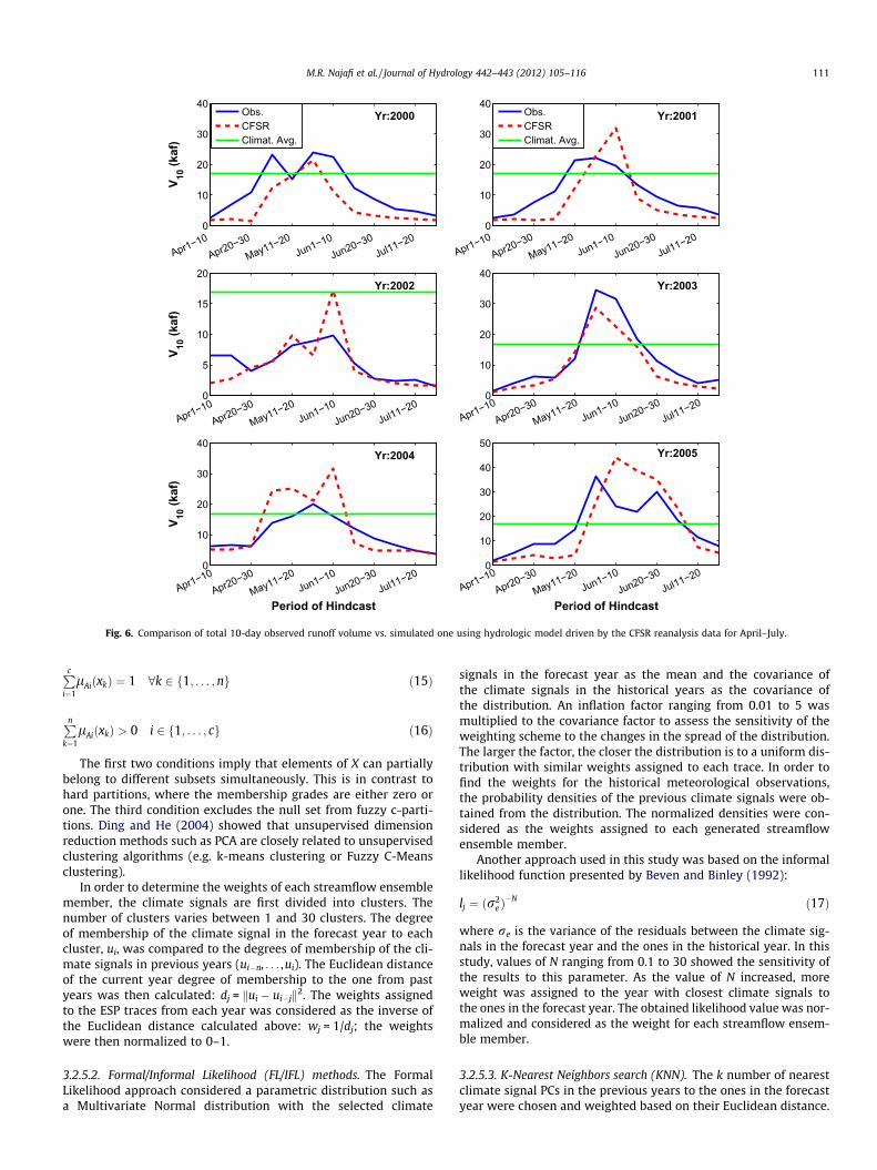
According to Fig. 2, the CFSR grid which lied in the East river ba-sin was used for the spring runoff simulation. Ten day runoff vol-umes during April–July (e.g. April 1st–10th, April 11th–20th, etc.)were calculated from the deterministic model runs using CFS data.The results were compared with observed values as well as the cli-matological averages (Fig. 6). The climatologic average was ob-tained by taking the mean of all 10 day volumetric runoffs from1976 to 1999. The model does capture the trend of observationand shows satisfactory results. The best performance was observed

ikelihood

me1993 1994 1995 1996 1997 1998 1999 2000

eighting approach in the training period.

Informal Likelihood

Time

Rel

ativ

e Er

ror

0.0

0.1

0.2

0.3

0.4

0.5

0.6

ESP_TraditionalAll PCsPRESSNRCS

1985 1986 1987 1988 1989 1990 1991 1992 1993 1994 1995 1996 1997 1998 1999 2000

Fig. 9. Performance of the Informal Likelihood weighting approach in the training period.

K−Nearest Neighbor

Time

Rel

ativ

e Er

ror

0.0

0.1

0.2

0.3

0.4

0.5

0.6

ESP_TraditionalAll PCsPRESSNRCS

1985 1986 1987 1988 1989 1990 1991 1992 1993 1994 1995 1996 1997 1998 1999 2000

1D−K−Nearest Neighbor

Time

Rel

ativ

e Er

ror

0.0

0.1

0.2

0.3

0.4

0.5

0.6

ESP_Traditional1st_PC

1985 1986 1987 1988 1989 1990 1991 1992 1993 1994 1995 1996 1997 1998 1999 2000

(a)

(b)

Fig. 10. Performance of the (a) K-Nearest Neighbor and (b) 1D-K-Nearest Neighbor weighting approaches in the training period.

M.R. Najafi et al. / Journal of Hydrology 442–443 (2012) 105–116 113

during the 2003 hindcast. For further investigation, CFSR data wasused as forcing data to the hydrologic model for deterministic sim-ulation of the volumetric spring runoff.

4. Results

This study considered any climate signal that has significantcorrelation with the spring runoff to apply in the ESP weightingscheme. The PCA was carried out to produce uncorrelated climatesignals and reduce the redundancy. A comparison made between

the ESPs weighted based on the climate signals and their principlecomponents revealed that in most cases the application of PCAwould enhance the weighting scheme considerably.

There were two unknown parameters in the weighting proce-dures including the number of climate signal PCs which was deter-mined based on the NRCS and PRESS approaches as discussedbefore and the second one was the applied coefficient. In orderto determine the optimal range of the coefficient values a trainingperiod of 1985–2000 was considered. In this period ESP wasweighted and compared with equal weight scenario based on

Table 2The simple averaging method vs. weighted average based on NRCS, bias corrected weighted average, deterministic CFSR run and the ESP based CFSR run for the test period of2001–2005.

Year Vobs Simple mean Before bias correction After bias correction CFSR Deterministic CFSR ESP

1D-KNN KNN FCM IFL FL 1D-KNN KNN FCM IFL FL

2001 127.31 97.64 97.64 96.09 97.6 98.52 96.03 127.91 125.99 127.85 129 125.91 98.6 93.372002 64.1 76.61 73.74 74.44 75.11 73.7 72.13 98.24 99.11 99.93 98.19 96.24 60.72 72.142003 142.32 93.4 96.73 93.13 97.42 93.76 100.81 126.77 122.31 127.64 123.09 131.84 109.69 94.922004 121.38 95.52 97.05 95.1 95.32 96.24 101.18 127.17 124.76 125.03 126.17 132.3 144.69 127.312005 189.85 157.3 162.64 158.17 163.17 164.3 160.95 208.61 203.06 209.27 210.68 206.51 194.78 175.86

114 M.R. Najafi et al. / Journal of Hydrology 442–443 (2012) 105–116

different coefficient values. The selected parameters were thenapplied for the test period of 2001–2005.

Considering the FCM method different number of clustersshowed varying results in the training period and for this particularregion a number of five clusters was ultimately chosen. Fig. 7shows the relative errors in the training years for four scenarios:ESP equal weight average, ESP weighted average considering dif-ferent values of PCs (i.e. from 1 to the total number of PCs), ESPweighted with number of PCs selected through PRESS and thenNRCS. In the case of different values of PCs, the minimum erroramong all numbers of PCs was shown. This expresses the influen-tial role of the number of PCs on the performance of weighting.This scenario was not applied for the test years since the minimumvalues are unknown. In this figure the relative error is defined as:

RE ¼ jVs � VobsjV

ð18Þ

where Vobs;Vs represent the observed spring runoff volume, andweighted and unweighted mean of the ensemble streamflowpredictions respectively. The weighting model reduced the relativeerror in several years including 1989, 1993 and 1997. Also the per-formance of the weighting method varied based on the number ofPCs selected using NRCS and PRESS approaches.

For this study a covariance inflation factor of �0.2 was chosenfor this basin. This was applied to the multivariate normal distribu-tion as a multiplicative factor as described in previous sections(Fig. 8). Number of PCs determined based on the PRESS methodprovide better results than the ones from NRCS. The results fromFL outperform the ones from FCM. A similar comparison was per-formed for the IFL approach (Fig. 9). With N = 5, this method pro-vided better results than the two previous methods for thetraining period. Significant improvements were made to the volu-metric prediction in 1990, 1993 and 1997 hindcasts as well as sev-eral other years. It should be noted that at least two principlecomponents were required to perform this weighting scheme tofind the variance of the residuals. Fig. 10a and b reflects the perfor-mances of the KNN and 1D-KNN approaches respectively. With 12nearest neighbors the KNN performance was acceptable.

In general the results showed that removing the co-linearity be-tween the climate signals via PCA improves the weighting scheme.The number of optimum PCs to retain is an important factor inreducing the ESP mean error. We applied the selected parametersfor the test period of 2001–2005 in order to evaluate the perfor-mance of the weighing procedure. Furthermore, a simple linear biascorrection was applied to the weighted averages in order to elimi-nate the negative biases in the predictions. Table 2 compares theobserved volumetric streamflow (in kaf) with different scenariosincluding the model run using CFSR data. The weighting resultswere based on the number of PCs chosen by the NRCS method. Over-all the predictions based on the ESP weighting show improvementsto the simple averaging of the ESP traces. Bias correction of the pre-dictions also significantly enhanced the ESP results. The hydrologic

model run using the new set of CFSR data provided promising volu-metric predictions for both deterministic and ESP scenarios.

5. Conclusions

Water resource managers require accurate and timely predic-tions of streamflow to allocate limited resources and meet oftencompeting demands for water. Seasonal streamflow forecastinghas important socio-economic implications and also direct impacton the design and operation of water resources systems. Currentlythe NWS issues seasonal volumetric streamflow predictions forvarious stakeholders as the mean or median of the ensemble fore-casts. However these approaches do not take into account thesignificant correlation between the climate signals and the runoffvolume, and treat all the resampled historical forcings equallywithout assigning any weights to them or even assigning weightsto streamflow ensemble members. On the other hand, using thesimple average causes bias towards the frequent climatologic con-dition. Moreover the similarity between climatologic variables indifferent years is ignored.

Enhancement of the streamflow prediction using climate sig-nals as additional information would directly benefit water re-sources managers in their decision making for water allocations.Climate signals were considered in this study as useful data setsin finding similarities between climate conditions in historical re-cords with the current year’s and use this information to applyweights to different streamflow ensemble members. To removethe correlation of the climate signals, and also summarize the data-set, Principle Component Analysis was applied. Further analysiswas performed to identify the optimal number of principle compo-nents to consider based on the NRCS and PRESS methods. Besides, atraining period of 1985–2000 was considered to determine theparameters used in each weighting method. The results indicatethat, in general, climate signals provide weights that can improvethe forecasts of the spring runoff volume considerably.

The application of the CFSR new analysis outperformed the con-ventional ESP in some years. The role of high resolution and accu-rate climate forecast as hydrologic model forcing is significant forlong term streamflow predictions. However, bias correction ofthe climate data seemed necessary before using them as forcingdata in hydrologic models. In this study the simple delta methodshowed better results than the quantile mapping and linear biascorrection methods.

The procedure presented here has the potential to be consideredin operational settings. The current predictions can be accompaniedwith the weighted ensemble forecasts to characterize the stream-flow forecast uncertainty bounds more accurately. Improvementin the weighting approach can be obtained by accurately selectingthe climate signals, choosing the right number of PCs and consider-ing various weighting techniques.

An alternative in selecting the climate signals is the Indepen-dent Component Analysis (ICA) (Moradkhani and Meier, 2010;

M.R. Najafi et al. / Journal of Hydrology 442–443 (2012) 105–116 115

Najafi et al., 2011c) where the dependence among the climate sig-nals can be removed. In fact, ICA has the decorrelation step asimplemented in PCA, however, it allows for generating indepen-dent signals. Application of a procedure to merge various predic-tions including weighted/non-weighted ESPs such as BayesianModel Averaging (Najafi et al., 2011a, 2011b) which accounts forthe uncertainties in the estimations would further enhance thestreamflow predictions.

Acknowledgement

Partial financial support for this research was provided byNOAA–CPPA, Grant No. NA07OAR4310203 NOAA–CSTAR, GrantNos. NA11NWS4680002, and NOAAMAPP, Grant No. NA11OAR4310140.

Appendix A

RPSt ¼PKk¼1½Pk

t � Okt �

2 ð1Þ

where Pkt and Ok

t are the forecast and observed probabilities at time tfor the kth category (Ck) respectively.

Pkt ¼

1Ne

PNe

i¼1cðysi

t < CkÞ ð2Þ

Okt ¼ cð�yt < CkÞ ð3Þ

where Ne is the ensemble size, and cðysit < CkÞ represents the num-

ber of ensemble members (ys) that are less than a threshold for eachtime step. Ok

t ¼ cð�yt < CkÞ is 1 if the mean observed runoff at timet(�yt) is less than the threshold and 0 otherwise.

RPSclimatology ¼1

Nd

PNd

t¼1

PKk¼1½Ok

t � O�2 ð4Þ

RPSS ¼ 1� RPS

RPSclimatologyð5Þ

Nd is the total number of measurements.

RPSSD ¼ 1� RPS

RPSclimatology þ Dð6Þ

D ¼ D0

Neð7Þ

D0 ¼PKk¼1

Pki¼1

pi 1� pi � 2Pk

j¼iþ1pj

!" #ð8Þ

where pi is the category probability and D is the intrinsic unreliabil-ity that provides the Debiased RPSS considering the limited numberof ensemble members. For K equiprobable categories:

pk ¼1k

ð9Þ

D0 ¼k2 � 1

6kð10Þ

References

Anderson, E.A., 1973. National Weather Service River Forecast System–SnowAccumulation and Ablation Model. Technical Memorandum Nws Hydro-17,November 1973, 217 p.

Anderson, E.A., 2002. Calibration of conceptual hydrologic models for use in riverforecasting. Rep. NWS Hydro. 17.

Beven, K., Binley, A., 1992. The future of distributed models: model calibration anduncertainty prediction. Hydrol. Process. 6 (3), 279–298.

Bezdek, J.C., Ehrlich, R., 1984. FCM: The fuzzy c-means clustering algorithm.Comput. Geosci. 10 (2–3), 191–203.

Burnash, R.J.C., 1995. The NWS river forecast system—catchment modeling.Comput. Models Watershed Hydrol., 311–366.

Burnash, R., Ferral, R., McGuire, R., 1973. A Generalised Streamflow SimulationSystem–Conceptual Modelling for Digital Computers. Joint Federal and StateRiver Forecast Center, Sacramento, Technical Report.

Clark, M.P., Hay, L.E., 2004. Use of medium-range numerical weather predictionmodel output to produce forecasts of streamflow. J. Hydrometeorol. 5 (1), 15–32.

Day, G.N., 1985. Extended streamflow forecasting using NWSRFS. J. Water Resour.Plan. Manage. 111 (2), 157–170.

DeChant, C., Moradkhani, H., 2011a. Radiance data assimilation for operationalsnow and streamflow forecasting. Adv. Water Resour. 34, 351–364.

DeChant, C., Moradkhani, H., 2011b. Improving the characterization of initialcondition for ensemble streamflow prediction using data assimilation. Hydrol.Earth Syst. Sci. 15, 3399–3410. http://dx.doi.org/10.5194/hess-15-3399-2011.

Ding, C., He, X., 2004. K-means Clustering via Principal Component Analysis. ACM,pp. 29.

Ebisuzaki, W., Zhang, L., 2011. Assessing the performance of the CFSR by anensemble of analyses. Clim. Dynam., 1–10.

Farnsworth, R.K., Thompson, E.S., Peck, E.L., 1982. Evaporation Atlas for theContiguous 48 United States. US Dept. of Commerce National Oceanic andAtmospheric Administration, National Weather Service.

Friedman, J.H., Bentley, J.L., Finkel, R.A., 1977. An algorithm for finding best matchesin logarithmic expected time. ACM Trans. Math. Softw. (TOMS) 3 (3), 209–226.

Garcia, V., Debreuve, E., Barlaud, M., 2008. Fast K Nearest Neighbor Search UsingGPU.

Grantz, K., Rajagopalan, B., Clark, M., Zagona, E., 2005. A technique for incorporatinglarge-scale climate information in basin-scale ensemble streamflow forecasts.Water Resour. Res. 41 (10), W10410.

Hamlet, A.F., Lettenmaier, D.P., 1999. Columbia River streamflow forecasting basedon ENSO and PDO climate signals. J. Water Resour. Plan. Manage. 125 (6), 333–341.

Hathaway, R.J., Bezdek, J.C., 2002. Fuzzy c-means clustering of incomplete data.Syst. Man Cybernetics Part B: Cybernetics IEEE Trans. 31 (5), 735–744.

Kennedy, A.M., Garen, D.C., Koch, R.W., 2009. The association between climateteleconnection indices and Upper Klamath seasonal streamflow: Trans-NiñoIndex. Hydrol. Process. 23 (7), 973–984.

Larson, L.W. et al., 1995. Operational responsibilities of the National WeatherService river and flood program. Weather Forecast. 10 (3), 465–476.

Laurine, D., Hughes, S., Younger, M., Orwig, C.E., 1996. Applying the NationalWeather Service River Forecast System (NWSRFS) Interactive Forecast Programto Basins in Northwest Washington.

Leisenring, M., Moradkhani, H., 2011. Snow water equivalent estimation usingBayesian data assimilation methods. Stoch. Environ. Res. Risk Assess. 25 (2),253–270.

Leung, L.R., Hamlet, A.F., Lettenmaier, D.P., Kumar, A., 1999. Simulations of the ENSOhydroclimate signals in the Pacific Northwest Columbia River basin. Bull. Amer.Meteorol. Soc. 80 (11), 2313–2330.

Li, H., Luo, L., Wood, E.F., Schaake, J., 2009. The role of initial conditions and forcinguncertainties in seasonal hydrologic forecasting. J. Geophys. Res. 114 (D4),D04114.

Madadgar, S., Moradkhani, H., Garen, D., 2012. Towards improved reliability andreduced uncertainty of hydrologic ensemble forecasts using multivariate post-processing. Hydrol. Process.

Madadgar, S., Moradkhani, H., in press. Drought analysis under climate changeusing copula. J. Hydrol. Eng. doi:10.1061/(ASCE)HE.1943-5584.0000532.

McEnery, J., Ingram, J., Duan, Q., Adams, T., Anderson, L., 2005. NOAA’s advancedhydrologic prediction service: building pathways for better science in waterforecasting. Bull. Am. Meteorol. Soc. 86 (3), 375–385.

Moradkhani, H., Meier, M., 2010. Long-lead water supply forecast using large-scaleclimate predictors and independent component analysis. J. Hydrol. Eng. 15 (10),744–762.

Moradkhani, H., Meskele, T., 2009. Probabilistic assessment of the satellite rainfallretrieval error translation to hydrologic response. In: Satellite Applications forSurface Hydrology. Water Science and Technology Library. Springer, pp. 229–242.

Moradkhani, H., Sorooshian, S., 2008. General review of rainfall-runoff modeling:model calibration. Data assimilation, and uncertainty analysis. In: HydrologicalModeling and Water Cycle. Coupling of the Atmospheric and HydrologicalModels. Water Science and Technology Library, Vol. 63. Springer, pp. 1–23.

Najafi, M., Moradkhani, H., Jung, I., 2011a. Assessing the uncertainties of hydrologicmodel selection in climate change impact studies. Hydrol. Process. 25 (18),2814–2826.

Najafi, M.R., Kavianpour, Z., Najafi, B., Kavianpour, M.R., Moradkhani, H., 2011b. Airdemand in gated tunnels – a Bayesian approach to merge various predictions.J. Hydroinformatics 14 (1), 152–166.

Najafi, M., Moradkhani, H., Wherry, S.A., 2011c. Statistical downscaling ofprecipitation using machine learning with optimal predictor selection.J. Hydrol. Eng. 16 (8), 650–664.

NWSRFS, 2005. User’s Manual Documentation. <http://www.nws.noaa.gov/oh/hrl/nwsrfs/users_manual/htm/xrfsdocpdf.php>.

116 M.R. Najafi et al. / Journal of Hydrology 442–443 (2012) 105–116

Parrish, M., Moradkhani, H., DeChant, C.M., 2012. Towards reduction of modeluncertainty: integration of Bayesian model averaging and data assimilation.Water Resour. Res. 48, W03519. http://dx.doi.org/10.1029/2011WR011116.

Regonda, S.K., Rajagopalan, B., Clark, M., Zagona, E., 2006. A multimodel ensembleforecast framework: application to spring seasonal flows in the Gunnison RiverBasin. Water Resour. Res. 42 (9), 9404.

Saha, S. et al., 2010. The NCEP climate forecast system reanalysis. Bull. Amer.Meteorol. Soc 91, 1015–1057.

Seo, D.J., Herr, H.D., Schaake, J.C., 2006. A statistical post-processor for accounting ofhydrologic uncertainty in short-range ensemble streamflow prediction. Hydrol.Earth Syst. Sci. Discuss. 3 (4), 1987–2035.

Smith, J.A., 1992. Nonparametric framework for long range streamflow forecasting.J. Water Resour. Plan. Manage. 118, 82.

Stephenson, D.B., Coelho, C.A.S., Doblas-Reyes, F.J., Balmaseda, M., 2005. Forecastassimilation: a unified framework for the combination of multi-model weatherand climate predictions. Tellus A 57 (3), 253–264.

Thirel, G., Rousset-Regimbeau, F., Martin, E., Habets, F., 2008. On the impact ofshort-range meteorological forecasts for ensemble streamflow predictions.J. Hydrometeorol. 9 (6), 1301–1317.

Timilsena, J., Piechota, T., Tootle, G., Singh, A., 2009. Associations of interdecadal/interannual climate variability and long-term Colorado River Basin streamflow.J. Hydrol. 365 (3–4), 289–301.

Twedt, T.M., Schaake, J.C., Peck, E.L., 1977. National Weather Service extendedstreamflow prediction. In: Proc. 45th Western Snow Conference, Albuquerque,pp. 52–57.

Weigel, A.P., Liniger, M.A., Appenzeller, C., 2007. Generalization of the discrete Brierand ranked probability skill scores for weighted multimodel ensembleforecasts. Mon. Weather Rev. 135 (7), 2778–2785.

Werner, K., Brandon, D., Clark, M., Gangopadhyay, S., 2004. Climate index weightingschemes for NWS ESP-based seasonal volume forecasts. J. Hydrometeorol. 5 (6),1076–1090.

Wilks, D.S., 2006. Comparison of ensemble-MOS methods in the Lorenz’96 setting.Meteorol. Appl. 13 (3), 243–256.

Wood, A.W., Kumar, A., Lettenmaier, D.P., 2005. A retrospective assessment ofNational Centers for Environmental Prediction climate model-based ensemblehydrologic forecasting in the western United States. J. Geophys. Res 110, 0148–0227.

Wood, A.W., Lettenmaier, D.P., 2006. A test bed for new seasonal hydrologicforecasting approaches in the western United States. Bull. Am. Meteorol. Soc. 87(12), 1699–1712.

Wood, A.W., Lettenmaier, D.P., 2008. An ensemble approach for attribution ofhydrologic prediction uncertainty. Geophys. Res. Lett. 35 (14), L14401.

Wood, A.W., Schaake, J.C., 2008. Correcting errors in streamflow forecast ensemblemean and spread. J. Hydrometeorol. 9 (1), 132–148.