Journal of Hydrology 399 (2011) 201–211

Contents lists available at ScienceDirect

Journal of Hydrology

journal homepage: www.elsevier .com/ locate / jhydrol

Enhancing PTFs with remotely sensed data for multi-scale soil waterretention estimation

Raghavendra B. Jana ⇑, Binayak P. MohantyDepartment of Biological and Agricultural Engineering, Texas A&M University, TX 77843-2117, United States

a r t i c l e i n f o

Article history:Received 14 April 2010Received in revised form 27 September2010Accepted 30 December 2010Available online 4 January 2011

This manuscript was handled by P. Baveye,Editor-in-Chief

Keywords:Bayesian Neural NetworksMultiscale methodsPedotransfer functionsRemote sensingDataNon-linear bias correction

0022-1694/$ - see front matter � 2011 Elsevier B.V. Adoi:10.1016/j.jhydrol.2010.12.043

⇑ Corresponding author. Address: Department ofEngineering, MS 2117, Texas A&M University, ColleUnited States. Tel.: +1 979 676 3427.

E-mail address: raghujana@tamu.edu (R.B. Jana).

s u m m a r y

Use of remotely sensed data products in the earth science and water resources fields is growing due toincreasingly easy availability of the data. Traditionally, pedotransfer functions (PTFs) employed for soilhydraulic parameter estimation from other easily available data have used basic soil texture and struc-ture information as inputs. Inclusion of surrogate/supplementary data such as topography and vegetationinformation has shown some improvement in the PTF’s ability to estimate more accurate soil hydraulicparameters. Artificial neural networks (ANNs) are a popular tool for PTF development, and are usuallyapplied across matching spatial scales of inputs and outputs. However, different hydrologic, hydro-cli-matic, and contaminant transport models require input data at different scales, all of which may notbe easily available from existing databases. In such a scenario, it becomes necessary to scale the soilhydraulic parameter values estimated by PTFs to suit the model requirements. Also, uncertainties inthe predictions need to be quantified to enable users to gauge the suitability of a particular dataset intheir applications. Bayesian Neural Networks (BNNs) inherently provide uncertainty estimates for theiroutputs due to their utilization of Markov Chain Monte Carlo (MCMC) techniques. In this paper, we pres-ent a PTF methodology to estimate soil water retention characteristics built on a Bayesian framework fortraining of neural networks and utilizing several in situ and remotely sensed datasets jointly. The BNN isalso applied across spatial scales to provide fine scale outputs when trained with coarse scale data. Ourtraining data inputs include ground/remotely sensed soil texture, bulk density, elevation, and Leaf AreaIndex (LAI) at 1 km resolutions, while similar properties measured at a point scale are used as fine scaleinputs. The methodology was tested at two different hydro-climatic regions. We also tested the effect ofvarying the support scale of the training data for the BNNs by sequentially aggregating finer resolutiontraining data to coarser resolutions, and the applicability of the technique to upscaling problems. TheBNN outputs are corrected for bias using a non-linear CDF-matching technique. Final results show goodpromise of the suitability of this Bayesian Neural Network approach for soil hydraulic parameter estima-tion across spatial scales using ground-, air-, or space-based remotely sensed geophysical parameters.Inclusion of remotely sensed data such as elevation and LAI in addition to in situ soil physical propertiesimproved the estimation capabilities of the BNN-based PTF in certain conditions.

� 2011 Elsevier B.V. All rights reserved.

1. Introduction

Remotely sensed data products have become increasingly avail-able for use in earth surface/water resources related research. TheNational Aeronautic and Space Administration (NASA) operates anumber of satellites which provide vital information about theearth’s surface processes. For example, the AQUA mission satellite,part of NASA’s Earth Observing System (EOS), has six instrumentson board which provide data regarding atmospheric and sea sur-face temperatures, humidity profiles, cloud data, precipitation,

ll rights reserved.

Biological and Agriculturalge Station, TX 77843-2117,

radiation balance, terrestrial snow, sea ice, and soil moisture,among others. Of particular interest are the Moderate-ResolutionImaging Spectrometer (MODIS) and the Advanced MicrowaveScanning Radiometer for EOS (AMSR-E) instruments. MODIS,which is also included on the TERRA satellite platform, providesproducts that include the Leaf Area Index (LAI) and other vegeta-tive indices such as the Normalized Difference Vegetative Index(NDVI) and land use land cover. AMSR-E provides a soil moisturedata product. With the easy availability of global scale remotelysensed data at different footprints or support scales, new applica-tions and scaling techniques for their utilization to hydrologicproblems have been investigated.

Pedotransfer functions (PTFs) have been used to obtain certaincomplex and expensive soil hydraulic parameters from otheravailable or easily measurable soil properties in the last two

202 R.B. Jana, B.P. Mohanty / Journal of Hydrology 399 (2011) 201–211

decades. Studies have been conducted to develop such transferfunctions and test them against available soil properties databases(e.g., Cosby et al., 1984; Rawls et al., 1991; van Genuchten and Leij,1992; Schaap and Bouten, 1996, 1998; Schaap and Leij, 1998a,b;Pachepsky et al., 1999; Wösten et al., 2001; Sharma et al., 2006;Jana et al., 2007, 2008). Traditionally, soil texture (%sand, %silt,%clay), and bulk density have been the predominant inputs in thesePTFs for prediction of soil hydraulic properties. However, usage ofsupplementary data in addition to texture and bulk density indeveloping pedotransfer functions has increased within the cur-rent decade. It has been shown that addition of topography andvegetation parameters enhance the predictive estimates of soilhydraulic parameters by PTFs to some extent (Pachepsky et al.,2001; Leij et al., 2004; Sharma et al., 2006). However, increasingthe number of model input parameters also means increasing thecomplexity of the model including the inherent uncertainties asso-ciated with the input data, and, consequently, the PTF estimates.

Artificial neural networks (ANNs) have been a preferred tool forparameter estimation by PTFs in hydrology (e.g., Schaap andBouten, 1996; Schaap et al., 1998; Schaap and Leij, 1998a; Sharmaet al., 2006; Jana et al., 2007, 2008). However, one major drawbackof using a conventional ANN approach is the inherent lack ofuncertainty estimates. This, in turn, brings to question the confi-dence one may place on the accuracy of the ANN predictions. Inone study, (Schaap et al., 1998) provided a posteriori estimates ofthe prediction uncertainties by generating multiple realizationsof the ANN output. The resultant outputs are then bootstrappedand analyzed to provide confidence levels. Another study by Janaet al. (2008) provided uncertainty estimates of the predicted soilhydraulic properties by using Bayesian Neural Networks whichare inherently designed to provide the confidence ranges. Conven-tionally, the weights of an ANN are obtained during training byiteratively adjusting the values till a single ‘‘optimal’’ set is ob-tained. However, the ANN methodology is not based on any phys-ical processes underlying the hydrology. Rather, the training of theweights in ANNs is a statistical process that is totally dependent onthe input values. Since most hydrologic systems are inherently sto-chastic, (Kingston et al., 2005), the existence of an ‘‘optimal’’ set ofweights is questionable.

Bayesian Neural Networks (BNNs) are designed to overcomethis deficiency in conventionally trained ANNs by obtaining arange of weights. Thus, a distribution of predicted values is gener-ated, explicitly accounting for the uncertainty in the predictions.Markov Chain Monte Carlo (MCMC) simulation techniques whichform a part of the BNN training also reduce the possibility of thetraining becoming stuck in local minima and overtraining of thenetwork. As such, BNNs incorporate the best features of conven-tional ANNs such as their ability to form functional relationshipsbetween the inputs and the targets, while addressing some of thedrawbacks such as the ability to provide stochastic limits. Thus,BNNs may be thought of as the next generation of neural networkmodels.

While the use of BNNs in the field of water resources modelingis still new, relatively little has been done towards using them forPTF development in the vadose zone. The utility of BNNs hasmostly been in surface hydrology applications where it has beenused for forecasting river salinity (Kingston et al., 2005), rainfall–runoff (Khan and Coulibaly, 2006), or oxygen demand in estuariesand coastal regions (Borsuk et al., 2001). Most previous PTF studiesderive and adopt soil hydraulic parameters at the same spatialscale of input and target data. (Jana et al., 2007, 2008) have dem-onstrated the usability of ANN- and BNN-based PTFs to estimatesoil water contents at a scale different from that of the trainingdata. The objective of this study is to develop and test the BayesianNeural Network based PTF methodology to derive soil water reten-tion values (at saturation, h0bar, and field capacity, h0.3bar) at differ-

ent scales using ground-based and remotely sensed data atmultiple scales which include soil texture, bulk density, elevationand Leaf Area Index (LAI). Remotely sensed data such as brightnesstemperature have been used to derive soil state variables such assoil moisture (Chang and Islam, 2000; Das and Mohanty, 2006).The novelty of this study lies in the use of such satellite-basedmeasurements of vegetation and elevation in addition to theground based soil data for the estimation of relatively time-invari-ant parameters such as soil water retention.

In addition, we also study the dependency of the derived soilwater retention values on the scale of the training data. In an ear-lier work, (Jana et al., 2007) tested the effect of varying the extentfrom which training data for an artificial neural network is ex-tracted. The study showed that there was no significant improve-ment in the ANN predictions at the fine scale with increase inthe number of training data points at the coarse scale resultingfrom widening of the spatial extent. In this study we test the effectof changing another component of the scale triplet (Blöschl andSivapalan, 1995) – the measurement support. The support area isthe region over which a measurement is valid. A test of the effectof the change in the measurement support was conducted bysequentially decreasing the support scale of the BNN training datafrom 1 km to 30 m.

2. Study areas and data

The Bayesian training methodology is tested in two different re-gions in USA. The first is the Las Cruces Trench site in the RioGrande basin of New Mexico and the second is in the SouthernGreat Plain Experiment 1997 (SGP97) hydrology experiment re-gion in Oklahoma. The test sites were chosen so as to provide vari-ety in terrain, land use characteristics, vegetation, soil types andsoil distribution patterns. At the same time, sufficient data at thefine scale is also available to validate the BNN predictions. Thesetest beds have been used in previous multiscale PTF studies (Janaet al., 2007, 2008), and as such, provide a reference against whichthe results of this new study may be compared. A brief descriptionof the test locations is given below for completeness.

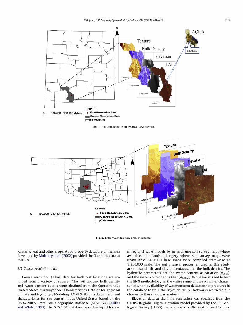
2.1. Rio Grande Basin

The Las Cruces Trench (Fig. 1) is located on the New MexicoState University Ranch, roughly 40 miles northeast of the Las Cru-ces city. The trench is situated in undisturbed soil on a basin slopeof Mt. Summerford, near the northern end of the Dona Ana Moun-tains. The region has a semi-arid climate and vegetation, with gen-erally flat topography. The trench is 26.4 m long, 4.5 m wide and6 m deep (Wierenga et al., 1991). Using in situ and laboratorymethods, Wierenga et al. (1989) developed a comprehensive data-base of fine-scale soil properties using 594 disturbed soil samplesand 594 associated soil cores taken from nine distinct soil layersidentified on the north wall of the trench. Samples were also takenfrom three vertical transects on this wall. The data set included sat-urated hydraulic conductivity, soil water retention function, parti-cle size distribution, and bulk density for each layer. Only the fiftydata points from the top 6-cm layer of the Las Cruces Trench sitedatabase is used in this study.

2.2. Little Washita Watershed

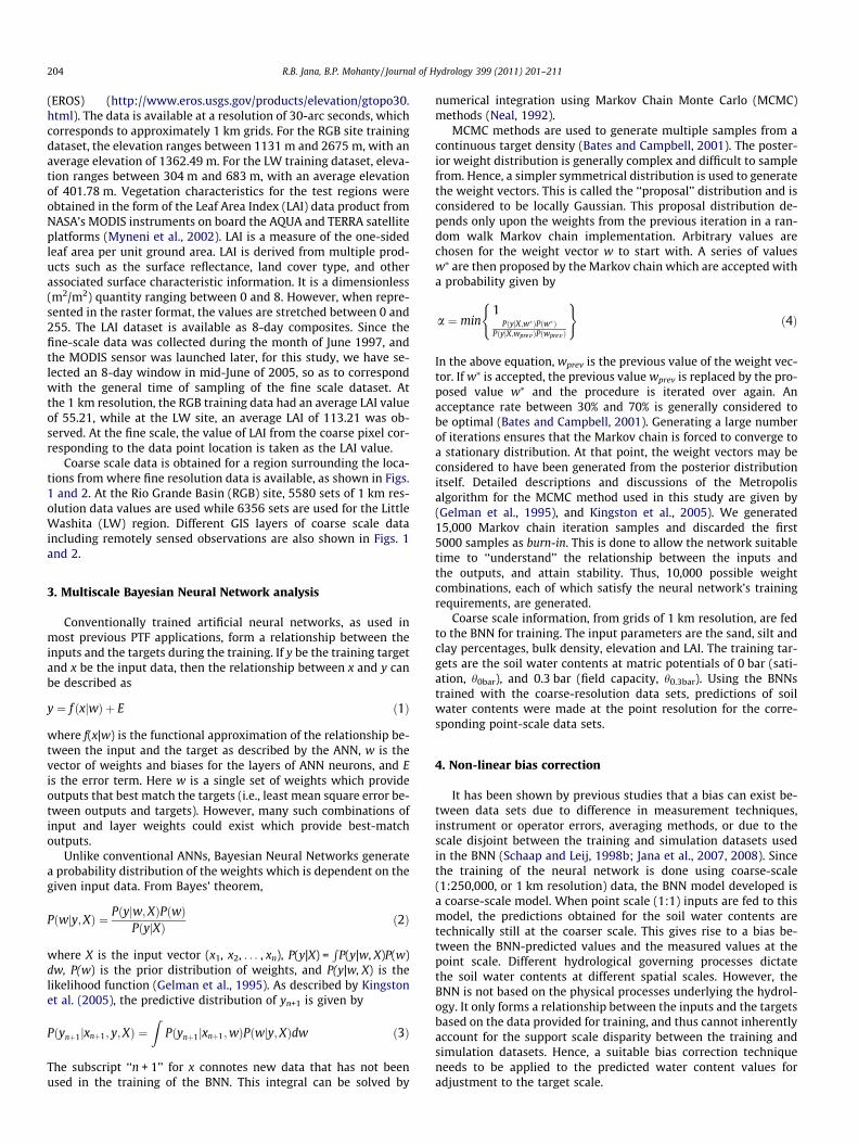
Fig. 2 shows the Southern Great Plains 97 (SGP97) experimentalregion of approximately 40 km by 250 km (10,000 km2) in the cen-tral part of the US Great Plains in the sub-humid environment ofOklahoma (Fig. 2). The region has a moderately rolling topography.Rangeland and pasture dominate the land use with patches of

Texture

Bulk Density

Elevation

LAI

AQUA

MODIS

Fig. 1. Rio Grande Basin study area, New Mexico.

Fig. 2. Little Washita study area, Oklahoma.

R.B. Jana, B.P. Mohanty / Journal of Hydrology 399 (2011) 201–211 203

winter wheat and other crops. A soil property database of the areadeveloped by Mohanty et al. (2002) provided the fine-scale data atthis site.

2.3. Coarse-resolution data

Coarse resolution (1 km) data for both test locations are ob-tained from a variety of sources. The soil texture, bulk densityand water content details were obtained from the ConterminousUnited States Multilayer Soil Characteristics Dataset for RegionalClimate and Hydrology Modeling (CONUS-SOIL), a database of soilcharacteristics for the conterminous United States based on theUSDA-NRCS State Soil Geographic Database (STATSGO) (Millerand White, 1998). The STATSGO database was developed for use

in regional scale models by generalizing soil survey maps whereavailable, and Landsat imagery where soil survey maps wereunavailable. STATSGO base maps were compiled state-wise at1:250,000 scale. The soil physical properties used in this studyare the sand, silt, and clay percentages, and the bulk density. Thehydraulic parameters are the water content at satiation (h0bar),and the water content at 1/3 bar (h0.3bar). While we wished to testthe BNN methodology on the entire range of the soil water charac-teristic, non-availability of water content data at other pressures inthe database to train the Bayesian Neural Networks restricted ourchoices to these two parameters.

Elevation data at the 1 km resolution was obtained from theGTOPO30 global digital elevation model provided by the US Geo-logical Survey (USGS) Earth Resources Observation and Science

204 R.B. Jana, B.P. Mohanty / Journal of Hydrology 399 (2011) 201–211

(EROS) (http://www.eros.usgs.gov/products/elevation/gtopo30.html). The data is available at a resolution of 30-arc seconds, whichcorresponds to approximately 1 km grids. For the RGB site trainingdataset, the elevation ranges between 1131 m and 2675 m, with anaverage elevation of 1362.49 m. For the LW training dataset, eleva-tion ranges between 304 m and 683 m, with an average elevationof 401.78 m. Vegetation characteristics for the test regions wereobtained in the form of the Leaf Area Index (LAI) data product fromNASA’s MODIS instruments on board the AQUA and TERRA satelliteplatforms (Myneni et al., 2002). LAI is a measure of the one-sidedleaf area per unit ground area. LAI is derived from multiple prod-ucts such as the surface reflectance, land cover type, and otherassociated surface characteristic information. It is a dimensionless(m2/m2) quantity ranging between 0 and 8. However, when repre-sented in the raster format, the values are stretched between 0 and255. The LAI dataset is available as 8-day composites. Since thefine-scale data was collected during the month of June 1997, andthe MODIS sensor was launched later, for this study, we have se-lected an 8-day window in mid-June of 2005, so as to correspondwith the general time of sampling of the fine scale dataset. Atthe 1 km resolution, the RGB training data had an average LAI valueof 55.21, while at the LW site, an average LAI of 113.21 was ob-served. At the fine scale, the value of LAI from the coarse pixel cor-responding to the data point location is taken as the LAI value.

Coarse scale data is obtained for a region surrounding the loca-tions from where fine resolution data is available, as shown in Figs.1 and 2. At the Rio Grande Basin (RGB) site, 5580 sets of 1 km res-olution data values are used while 6356 sets are used for the LittleWashita (LW) region. Different GIS layers of coarse scale dataincluding remotely sensed observations are also shown in Figs. 1and 2.

3. Multiscale Bayesian Neural Network analysis

Conventionally trained artificial neural networks, as used inmost previous PTF applications, form a relationship between theinputs and the targets during the training. If y be the training targetand x be the input data, then the relationship between x and y canbe described as

y ¼ f ðxjwÞ þ E ð1Þ

where f(x|w) is the functional approximation of the relationship be-tween the input and the target as described by the ANN, w is thevector of weights and biases for the layers of ANN neurons, and Eis the error term. Here w is a single set of weights which provideoutputs that best match the targets (i.e., least mean square error be-tween outputs and targets). However, many such combinations ofinput and layer weights could exist which provide best-matchoutputs.

Unlike conventional ANNs, Bayesian Neural Networks generatea probability distribution of the weights which is dependent on thegiven input data. From Bayes’ theorem,

Pðwjy;XÞ ¼ Pðyjw;XÞPðwÞPðyjXÞ ð2Þ

where X is the input vector (x1, x2, . . . , xn), P(y|X) =R

P(y|w, X)P(w)dw, P(w) is the prior distribution of weights, and P(y|w, X) is thelikelihood function (Gelman et al., 1995). As described by Kingstonet al. (2005), the predictive distribution of yn+1 is given by

Pðynþ1jxnþ1; y;XÞ ¼Z

Pðynþ1jxnþ1;wÞPðwjy;XÞdw ð3Þ

The subscript ‘‘n + 1’’ for x connotes new data that has not beenused in the training of the BNN. This integral can be solved by

numerical integration using Markov Chain Monte Carlo (MCMC)methods (Neal, 1992).

MCMC methods are used to generate multiple samples from acontinuous target density (Bates and Campbell, 2001). The poster-ior weight distribution is generally complex and difficult to samplefrom. Hence, a simpler symmetrical distribution is used to generatethe weight vectors. This is called the ‘‘proposal’’ distribution and isconsidered to be locally Gaussian. This proposal distribution de-pends only upon the weights from the previous iteration in a ran-dom walk Markov chain implementation. Arbitrary values arechosen for the weight vector w to start with. A series of valuesw⁄ are then proposed by the Markov chain which are accepted witha probability given by

a ¼ min1

PðyjX;w�ÞPðw�ÞPðyjX;wprev ÞPðwprev Þ

( )ð4Þ

In the above equation, wprev is the previous value of the weight vec-tor. If w⁄ is accepted, the previous value wprev is replaced by the pro-posed value w⁄ and the procedure is iterated over again. Anacceptance rate between 30% and 70% is generally considered tobe optimal (Bates and Campbell, 2001). Generating a large numberof iterations ensures that the Markov chain is forced to converge toa stationary distribution. At that point, the weight vectors may beconsidered to have been generated from the posterior distributionitself. Detailed descriptions and discussions of the Metropolisalgorithm for the MCMC method used in this study are given by(Gelman et al., 1995), and Kingston et al., 2005). We generated15,000 Markov chain iteration samples and discarded the first5000 samples as burn-in. This is done to allow the network suitabletime to ‘‘understand’’ the relationship between the inputs andthe outputs, and attain stability. Thus, 10,000 possible weightcombinations, each of which satisfy the neural network’s trainingrequirements, are generated.

Coarse scale information, from grids of 1 km resolution, are fedto the BNN for training. The input parameters are the sand, silt andclay percentages, bulk density, elevation and LAI. The training tar-gets are the soil water contents at matric potentials of 0 bar (sati-ation, h0bar), and 0.3 bar (field capacity, h0.3bar). Using the BNNstrained with the coarse-resolution data sets, predictions of soilwater contents were made at the point resolution for the corre-sponding point-scale data sets.

4. Non-linear bias correction

It has been shown by previous studies that a bias can exist be-tween data sets due to difference in measurement techniques,instrument or operator errors, averaging methods, or due to thescale disjoint between the training and simulation datasets usedin the BNN (Schaap and Leij, 1998b; Jana et al., 2007, 2008). Sincethe training of the neural network is done using coarse-scale(1:250,000, or 1 km resolution) data, the BNN model developed isa coarse-scale model. When point scale (1:1) inputs are fed to thismodel, the predictions obtained for the soil water contents aretechnically still at the coarser scale. This gives rise to a bias be-tween the BNN-predicted values and the measured values at thepoint scale. Different hydrological governing processes dictatethe soil water contents at different spatial scales. However, theBNN is not based on the physical processes underlying the hydrol-ogy. It only forms a relationship between the inputs and the targetsbased on the data provided for training, and thus cannot inherentlyaccount for the support scale disparity between the training andsimulation datasets. Hence, a suitable bias correction techniqueneeds to be applied to the predicted water content values foradjustment to the target scale.

R.B. Jana, B.P. Mohanty / Journal of Hydrology 399 (2011) 201–211 205

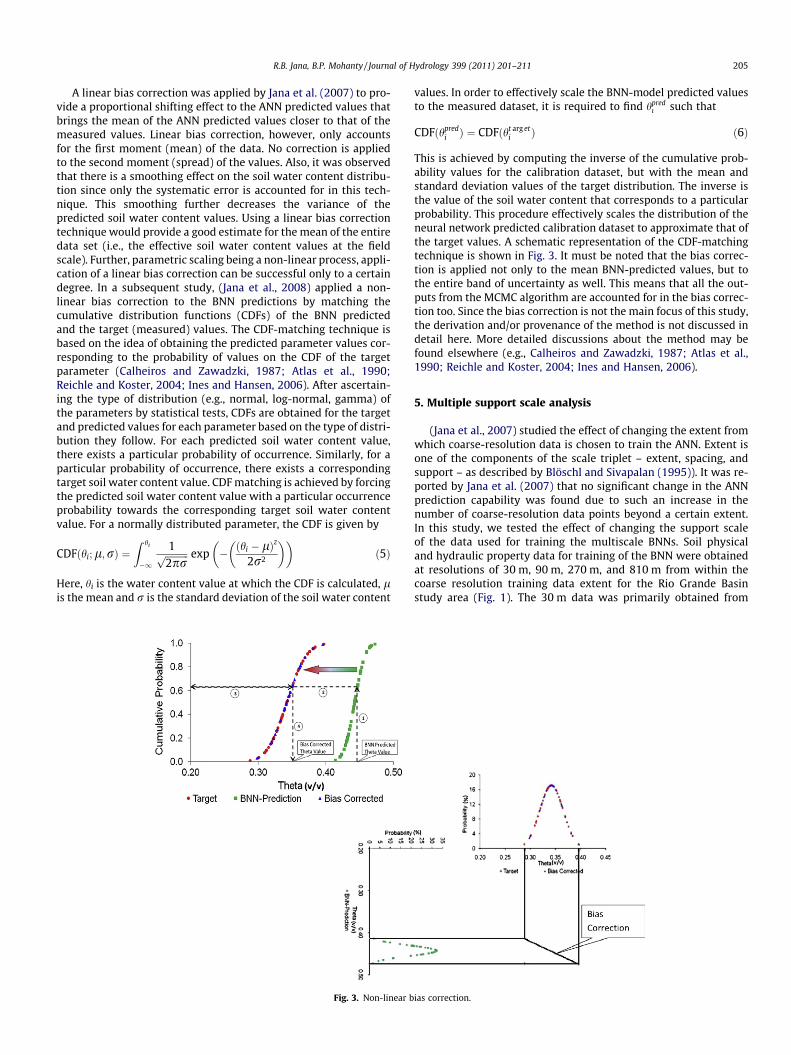
A linear bias correction was applied by Jana et al. (2007) to pro-vide a proportional shifting effect to the ANN predicted values thatbrings the mean of the ANN predicted values closer to that of themeasured values. Linear bias correction, however, only accountsfor the first moment (mean) of the data. No correction is appliedto the second moment (spread) of the values. Also, it was observedthat there is a smoothing effect on the soil water content distribu-tion since only the systematic error is accounted for in this tech-nique. This smoothing further decreases the variance of thepredicted soil water content values. Using a linear bias correctiontechnique would provide a good estimate for the mean of the entiredata set (i.e., the effective soil water content values at the fieldscale). Further, parametric scaling being a non-linear process, appli-cation of a linear bias correction can be successful only to a certaindegree. In a subsequent study, (Jana et al., 2008) applied a non-linear bias correction to the BNN predictions by matching thecumulative distribution functions (CDFs) of the BNN predictedand the target (measured) values. The CDF-matching technique isbased on the idea of obtaining the predicted parameter values cor-responding to the probability of values on the CDF of the targetparameter (Calheiros and Zawadzki, 1987; Atlas et al., 1990;Reichle and Koster, 2004; Ines and Hansen, 2006). After ascertain-ing the type of distribution (e.g., normal, log-normal, gamma) ofthe parameters by statistical tests, CDFs are obtained for the targetand predicted values for each parameter based on the type of distri-bution they follow. For each predicted soil water content value,there exists a particular probability of occurrence. Similarly, for aparticular probability of occurrence, there exists a correspondingtarget soil water content value. CDF matching is achieved by forcingthe predicted soil water content value with a particular occurrenceprobability towards the corresponding target soil water contentvalue. For a normally distributed parameter, the CDF is given by

CDFðhi; l;rÞ ¼Z hi

�1

1ffiffiffiffiffiffiffiffiffiffi2prp exp � ðhi � lÞz

2r2

� �� �ð5Þ

Here, hi is the water content value at which the CDF is calculated, lis the mean and r is the standard deviation of the soil water content

Fig. 3. Non-linear b

values. In order to effectively scale the BNN-model predicted valuesto the measured dataset, it is required to find hpred

ı such that

CDFðhpredi Þ ¼ CDFðht arg et

i Þ ð6Þ

This is achieved by computing the inverse of the cumulative prob-ability values for the calibration dataset, but with the mean andstandard deviation values of the target distribution. The inverse isthe value of the soil water content that corresponds to a particularprobability. This procedure effectively scales the distribution of theneural network predicted calibration dataset to approximate that ofthe target values. A schematic representation of the CDF-matchingtechnique is shown in Fig. 3. It must be noted that the bias correc-tion is applied not only to the mean BNN-predicted values, but tothe entire band of uncertainty as well. This means that all the out-puts from the MCMC algorithm are accounted for in the bias correc-tion too. Since the bias correction is not the main focus of this study,the derivation and/or provenance of the method is not discussed indetail here. More detailed discussions about the method may befound elsewhere (e.g., Calheiros and Zawadzki, 1987; Atlas et al.,1990; Reichle and Koster, 2004; Ines and Hansen, 2006).

5. Multiple support scale analysis

(Jana et al., 2007) studied the effect of changing the extent fromwhich coarse-resolution data is chosen to train the ANN. Extent isone of the components of the scale triplet – extent, spacing, andsupport – as described by Blöschl and Sivapalan (1995)). It was re-ported by Jana et al. (2007) that no significant change in the ANNprediction capability was found due to such an increase in thenumber of coarse-resolution data points beyond a certain extent.In this study, we tested the effect of changing the support scaleof the data used for training the multiscale BNNs. Soil physicaland hydraulic property data for training of the BNN were obtainedat resolutions of 30 m, 90 m, 270 m, and 810 m from within thecoarse resolution training data extent for the Rio Grande Basinstudy area (Fig. 1). The 30 m data was primarily obtained from

ias correction.

206 R.B. Jana, B.P. Mohanty / Journal of Hydrology 399 (2011) 201–211

the Soil Survey Geographic (SSURGO) database compiled by theUnited States Department of Agriculture – Natural Resources Con-servation Service (USDA-NRCS) (http://soildatamart.nrcs.usda.gov). This public domain database contains geo-referenced spatialand attribute data for soils compiled from soil surveys. These sur-veys cover large spatial extents (usually county-wide) and the soilproperty data are based on soil type rather than the spatial loca-tion. The SSURGO database was created by field methods, usingobservations along soil delineation boundaries and traverses, anddetermining map unit composition by field transects. Aerial photo-graphs are interpreted and used as the field map base. Multiplereadings are taken for each property within each map unit. Thenumber of readings taken differs between map units that are basedon factors such as the size of the soil polygon, the variation intopography and change in vegetation, among others. Low, high,and representative values for each soil physical and/or hydraulicproperty are provided in the database for each soil type/map unitat scales ranging between 1:12,000 and 1:31,680 (http://www.nrcs.usda.gov/technical/soils/soilfact.html). In this study, the rep-resentative values for the soil texture (sand, silt and clay percent-ages), bulk density, elevation, and soil water contents wereobtained from 1:24,000 resolution SSURGO soil maps in a griddedformat with a resolution of 30 m. The LAI values were re-sampledfrom the MODIS data described earlier.

The 3 � 3 grids of parametric data at the 30 m resolution aregeneralized to 90 m resolution using the mean aggregation featurein ArcMap™ software by ESRI�. The 270 m resolution data was ob-tained by aggregating 3 � 3 grids of 90 m data, and so on. Since thesoil property data are in grid format, changing the support area ofthe parameter causes a corresponding change in the spacing too.Hence, in reality, two components of the scale triplet are beingmodified here.

The BNN methodology, along with the non-linear biascorrection technique, was applied with the BNN being trained withdata at each coarse resolution. Predictions of the soil watercontents at saturation and field capacity at the point (1:1) resolu-tion were obtained, and corrected for bias by the CDF mappingmethod.

Fig. 4. Target, BNN-predicted, and bias c

6. Upscaling study

In order to investigate the multi-scale nature of the BayesianNeural Networks, a study was conducted to upscale the soil waterretention parameters from the 30 m resolution to the 1 km resolu-tion at the Little Washita Watershed site. Training data at the 30 mresolution for this study consisted of the soil texture (sand, silt andclay percentages), and the bulk density from the USDA-NRCS SSUR-GO database. Elevation data obtained at the 30 m resolution fromthe United States Geological Survey’s (USGS) National ElevationDataset was also used as a training input. Training targets werethe water content at satiation (h0bar) and the water content at 1/3 bar (h0.3bar). Simulation input data for soil texture and bulk den-sity at the 1 km resolution were obtained from the STATSGO data-base, while the elevation data were from the GTOPO30 globaldigital elevation model mentioned earlier.

Twelve coarse resolution (1 km) pixels were taken from the LWregion for this study. Fine (30 m) resolution training input and tar-get data from within these areas were taken from the SSURGO andNational Elevation databases. The BNN methodology was appliedwith the networks being trained at the fine scale. Predictions ofthe soil water contents at saturation and field capacity at thecoarse (1 km) resolution were then obtained.

7. Results and discussion

Data from multiple scales, from satellite-based remote sensingfootprints to ground-based point scale measurements, were ap-plied in a multiscale Bayesian Neural Network methodology to ob-tain fine-scale soil water content values after being trained withcoarse scale data. The resultant outputs from the BNN were plottedalong with their respective expected values (Fig. 4). The error bars,obtained from the Markov chain Monte Carlo simulations, repre-sent the uncertainty in the neural network predictions. BNNs, asmentioned earlier, generate a distribution of weights instead of asingle set. The uncertainty band (error bars) show the limits towhich the predictions could have varied based on the combination

orrected soil water content values.

R.B. Jana, B.P. Mohanty / Journal of Hydrology 399 (2011) 201–211 207

of weights used. The final predicted soil water content value is anaverage of all such possible values from the 1000 Monte Carlo sim-ulations. Fifty sets of point scale inputs/outputs are available foreach parameter at the Rio Grande Basin (RGB), while in the LittleWashita Watershed (LW), we have seventy values measured atthe point scale. The comparative statistics for the target and pre-dicted parameters at the two sites are given in Table 1. As ex-pected, BNN predictions at both test sites and for both watercontent parameters were biased from the expected target values.As previously noted, this bias is an artifact of the scale disjoint be-tween the training and simulation data sets, and is eliminated byapplication of the non-linear bias correction technique.

As in the study by Jana et al. (2008), it is apparent that the out-puts at the RGB site showed less variations than those at the LWsite (Fig. 4). This relative invariance is attributed to the small rangein variations of the corresponding inputs at the fine scale. Descrip-tive statistics for the soil physical properties at the coarse and finescales from the two test sites are presented in Table 2. There is asignificant difference in the amount of variation of the texture be-tween the coarse and fine scales at RGB. The fine-scale soil is pre-dominantly sandy and almost uniform. Further, the Las Crucestrench has a dimension of 26 m. This means that all the observa-tion points at this site lie within one coarse scale pixel, thus show-ing invariance in topography and vegetation too. Like any othermodel, neural network outputs too are dependent on the qualityof input data. The invariance in the inputs at the fine scale is re-flected in the soil water content estimates produced by the BNN.In contrast, the LW data are spread over a much wider area(approximately 10,000 km2). Fine scale observation points lie indifferent coarse scale pixels. The variability in the soil physicalproperties are also comparable at the two scales (Table 2). This re-sults in a better estimation of the water content values at the LWsite as compared to the RGB site, as can be seen from the R valuesin Table 1.

Table 1Descriptive and comparative statistics of target, BNN-predicted, and Bias Correctedsoil water content values.

h0bar (v/v) h0.3bar (v/v)

Target BNN-predicted

Biascorrected

Target BNN-predicted

Biascorrected

RGBMean 0.342 0.443 0.342 0.127 0.418 0.127Std. dev. 0.024 0.012 0.024 0.013 0.011 0.013R 0.328 0.333 0.223 0.257RMSE 0.103 0.026 0.246 0.015

LWMean 0.370 0.414 0.370 0.210 0.533 0.210Std. dev. 0.046 0.019 0.046 0.064 0.111 0.064R 0.416 0.421 0.762 0.764RMSE 0.061 0.050 0.331 0.044

RGB: Rio Grande Basin; LW: Little Washita; BNN: Bayesian Neural Network; R:Correlation coefficient; RMSE: Root mean square error.

Table 2Bayesian Neural Network input parameters at coarse and fine scales.

Sand (%) Silt (%) Clay (%)

Mean Std. dev. Mean Std. dev. Mean Std. de

RGBCoarse scale 54.641 13.973 30.603 7.796 14.752 7.751Fine scale 81.458 1.666 9.760 1.170 8.780 1.200

LWCoarse scale 41.969 17.280 43.875 14.034 14.226 5.726Fine scale 51.913 21.113 33.606 16.412 14.482 6.040

RGB: Rio Grande Basin; LW: Little Washita; LAI: Leaf Area Index.

From Table 1, for the RGB region, we see that the BNN estima-tion of the water content at saturation (h0bar) is slightly better thanthat for the field capacity (h0.3bar). A correlation coefficient value of0.333 is observed for the h0bar value, while the value is 0.257 forh0.3bar. Earlier studies (Jana et al., 2008) have shown similar corre-lation values. No significant improvement or deterioration in theBNN’s prediction capabilities were seen for the RGB site althoughthe resolution of the training data is much coarser (1 km) in thisstudy as compared to the earlier study (30 m), and considering thattopography and vegetation have been added to the training factors.We suggest that this is due to the general conditions of the RGBsite. This site exhibited more uniformity in soil texture, topogra-phy, and vegetation with large spatial correlation length scalewhen compared to the LW site.

For the LW site, the R value for the h0bar, at 0.421, remains sim-ilar to the earlier study (Jana et al., 2008). The correlation value forthe h0.3bar, however, is greatly improved (0.764). This improvementin the correlation can be attributed to the use of the topographicinformation in this model, as against using only texture and bulkdensity. Field capacity (h0.3bar) is defined as the available watercontent in the soil after gravity draining. Drainage by gravity, espe-cially from the wet end of the soil water characteristic, is greatlyinfluenced by the topography. By including the elevation in theBNN model, a better estimate of the variability is obtained for thisparameter as compared to the earlier study (Jana et al., 2008).

Kolmogorov–Smirnov tests showed that the BNN predicted andfield measured fine scale water content values are normally dis-tributed. Hence, the CDF matching algorithm for non-linear biascorrection could be carried out using the normal CDF equation(Eq. (5)). Normal CDFs were plotted for the target and predictedh values for both the regions (Fig. 5). It can be seen that the CDFsof the model predicted soil water content values and those of themeasured (target) values do not match for either region. Probabil-ity Density Functions (PDFs) are also plotted for the target andBNN-predicted h values for both the regions (Fig. 6). The differencein the mean and spread of the target and BNN-predicted distribu-tions is apparent here. The means of the BNN-predicted values areconsistently higher than the measured values for each water con-tent at either location. The BNN-predicted h values were randomlysplit into two halves, one half for model calibration and the otherfor validation of the bias correction scheme. The cumulative prob-abilities for each point value are computed using the mean andstandard deviation of the calibration dataset. The calibrated (biascorrected) soil water content CDF values (Fig. 5) now follow thetarget CDF closely.

To test the calibration of the bias correction scheme, theremaining half of the neural network predicted soil water contentvalues (the validation dataset) is used. The calibration is found tobe correct as the distributions of validation data are aligned withthe target distributions (Fig. 5). This suggests that our bias correc-tion scheme for the predicted h values approximates the target val-ues well. In concurrence with the CDFs, the PDFs of the calibration

Bulk density (–) Elevation (m) LAI (m2/m2)

v. Mean Std. dev. Mean Std. dev. Mean Std. dev.

1.520 0.174 1362.490 167.060 55.210 19.8741.660 0.050 1200.000 0.000 250.000 0.000

1.437 0.015 401.783 45.431 113.210 15.2721.396 0.099 391.000 25.213 12.400 2.815

Fig. 5. Cumulative probability distributions of soil water content values.

Fig. 6. Probability distributions of soil water content values.

208 R.B. Jana, B.P. Mohanty / Journal of Hydrology 399 (2011) 201–211

and validation datasets plot on top of the target PDF (Fig. 6). Scatterplots of the target, BNN-Prediction, calibration and validation val-ues for both water contents at both sites are also plotted (Fig. 7) toprovide a sense of how the bias correction procedure shifts theBNN predictions closer to the targets.

From Fig. 4 it can be seen that the variability of the target valuesis largely approximated by the non-linear bias-corrected h values.However, point-to-point matching of values is still not obtained.The bias-corrected values are being sampled from the same distri-bution as the target values, but at a different probability. Uncer-

tainties introduced into the observations of any point-scale datadue to measurement and operator errors, and other influencingfactors such as the presence of macropores or roots debris havenot been considered here. These factors make the approximationof the particular point values dictated by stochastic natural pro-cesses a near-impossible task, given the current inputs. Since theindividual values may also be considered as being sampled froma distribution (to cover the uncertainties), the point-to-pointmatch of the values is neither practically achievable nor reallynecessary. In other words, if we select values from the normal

Fig. 7. Scatter plots of soil water content values.

R.B. Jana, B.P. Mohanty / Journal of Hydrology 399 (2011) 201–211 209

distribution of the bias-corrected values for the exact probabilitiesas those of the target values, we would get a much better match ateach point. Further, uncertainties in fine-scale data due to factorssuch as measurement and/or operator errors and presence of mac-ropores or organic debris make it nearly impossible to preciselyestimate the observed values. The non-linear bias correction ap-proach provides h values for any probability, which is not possibleby using a linear bias correction. Matching of the distributions,along with the Bayesian nature of the neural network model, en-sures that the above-mentioned uncertainties are incorporatedinto the estimation scheme.

The mean, standard deviation, root mean square error (RMSE)and average bias correction applied to the predicted h values fromBNNs trained with data from different coarse resolutions (supportscales) in the multiple support scale analysis are given in Table 3.The average bias corrections applied at different resolutions aregraphed in Fig. 8. It is found that a fourth order polynomial fitsthe average bias correction curve with an R2 of 1 for both h values.We have used a non-linear bias correction based on the assump-tion that scaling is a non-linear process. The findings shown inFig. 8 support this assumption. If the effect of scale on the BNN pre-

Table 3Average bias correction necessary for different scales of training data.

h0bar (v/v) Target 30 m 90 m

Pred BC Pred BC

RGBMean 0.342 0.482 0.342 0.447 0.342Std. dev. 0.023 0.006 0.023 0.012 0.023Avg. BC �0.140 �0.105

LWMean 0.127 0.405 0.127 0.582 0.127Std. dev. 0.013 0.003 0.013 0.012 0.013Avg. BC �0.278 �0.455

h: Soil water content; Pred: BNN Predicted value; BC: Bias-corrected value; Avg. BC: Av

diction were to be linear, we would find that the average bias cor-rection rises linearly with increase in resolution. Further, the non-monotonic nature of the curve may be an indicator of the fractal/self-similar nature of the hydraulic property itself.

The target (from STATSGO) and BNN-predicted values for thewater content values at the 1 km resolution from the upscalingstudy are plotted in Fig. 9. It can be seen that the BNN-predictedwater content values are close to the target values at all locations.The target h0bar values fall within the band of uncertainty at alllocations, while the target h0.3bar values lie within the uncertaintyband at most (10/12) locations. Comparative statistics betweenthe target and BNN-predicted values are given in Table 4. It canbe seen that the correlation values are much higher for the upscal-ing study than for the downscaling case, and the RMSE is muchsmaller for both water content values. This shows that the upscal-ing was successful.

It may be observed that the bias correction was not applied inthe upscaling study. It was not considered necessary since upscal-ing is an interpolative exercise for the BNN. Neural networks per-form better at interpolation than they do at extrapolation. Thisinherent property of BNN’s means that they are naturally better

270 m 810 m 1 km

Pred BC Pred BC Pred BC

0.486 0.342 0.424 0.342 0.443 0.3420.016 0.023 0.011 0.023 0.012 0.024

�0.144 �0.082 �0.100

0.537 0.127 0.570 0.127 0.418 0.1270.012 0.013 0.014 0.013 0.011 0.013

�0.410 �0.443 �0.012

erage bias correction applied.

Fig. 8. Average bias correction necessary for different scales of training data.

Fig. 9. Target and BNN-predicted soil water content values at 1 km resolution from upscaling study.

Table 4Descriptive and comparative statistics of target, and BNN-predicted soil water contentvalues at 1 km resolution from upscaling study.

h0bar (v/v) h0.3bar (v/v)

Target BNN-predicted Target BNN-predicted

Mean 0.397 0.377 0.230 0.228Std. dev. 0.026 0.020 0.060 0.049R 0.598 0.802RMSE 0.028 0.035

210 R.B. Jana, B.P. Mohanty / Journal of Hydrology 399 (2011) 201–211

at upscaling exercises than downscaling, where an additional biascorrection step would be necessary to account for the scaledisjoint.

Remotely sensed data products are becoming increasingly easyto obtain and newer applications are being developed. The qualityof remotely sensed data is improving all the time. However, at thepresent time, the resolutions at which such data are available arestill rather coarse. This results in our having to resample the coarseresolution pixels to finer resolutions. Such simple resamplingmethods are not a substitute to rigorous scaling techniques, andintroduce errors in parametric values. Empirical PTFs based onstatistical techniques such as neural networks are inherentlysite-specific as they need to be trained to recognize the patternsparticular to that site. So a network would need to be trained freshif estimating soil hydraulic parameters at a site outside the areafrom which the coarse scale data is provided. Alternatively, thenetwork would need to be trained with a very comprehensivedataset encompassing all possible variability in soil physical prop-erties in order to be considered as a generic pedotransfer function

application. Further, using this methodology, a few representativemeasurements are necessary at the fine scale for the bias correc-tion procedure when downscaling the soil water retention param-eters. Using these measurements, an estimate of the amount ofcorrection to be applied can be obtained which can then be usedfor the entire extent of interest. However, this step is not necessaryfor upscaling the water retention parameters.

8. Conclusions

Using coarse scale soil properties data from ground-based andremote sensing platforms up to 1 km resolution and point scalemeasured soil properties data, we have shown that a BayesianNeural Network can be applied across spatial scales to approxi-mate fine-scale soil hydraulic properties. The study was conductedfor two regions which are greatly different in soil, topography, veg-etation, climate, and in the spatial extent from which the pointdata was collected. It has been shown that the BNN predictionsare superior when the training data covers a larger region. This isdue to the large scale heterogeneity encompassed in the trainingprocess. Using remotely sensed topographical and vegetationparameters in the training showed improvements in the LittleWashita region where the point scale inputs are from a widely dis-persed region. On the contrary, no significant improvement wasfound by the inclusion of additional parameters in the BNN train-ing at the Rio Grande Basin site where it is limited to a smalltrench/plot. A marked improvement in predicted h0.3bar valueswas found at the LW site, and is attributed to the inclusion of theadditional factors such as topography which represents the gravitydraining component. As expected, the scale disjoint between train-ing and simulation data made the application of a bias correction

R.B. Jana, B.P. Mohanty / Journal of Hydrology 399 (2011) 201–211 211

procedure necessary. The non-linear technique of CDF matchingwas used to obtain the bias correction. The average bias correctionnecessary to be applied was found to vary as a fourth order poly-nomial based on the resolution of the training data. BNNs also eas-ily provide an estimate of the uncertainties involved in theprediction scheme. Traditional ANN methods would involve afew further steps to obtain an a posteriori estimate of the sameuncertainties. Overall, the Bayesian Neural Network, coupled witha non-linear bias correction scheme, appears to work well for esti-mation of soil hydraulic properties at a fine scale from data at coar-ser scales (downscaling). The Bayesian Neural Networks performedbetter at upscaling of water retention parameters than at down-scaling, due to the inherent properties of the networks. However,this study also underlines the necessity of better input and trainingdata using remote sensing techniques for better predictions, as alsothe fact that no single model is applicable at all geographicallocations. Also, the currently available coarse scale data allowsfor testing of this approach only at the wet end of the soil watercharacteristic. If more points on the soil water characteristic curveare known at the coarse scale, then a comprehensive test of themethodology would be possible.

Acknowledgements

We acknowledge the partial support of Los Alamos NationalLab, NASA Earth System Science Fellowship (NNX06AF95H), Na-tional Science Foundation (CMG/DMS Grant 0621113) and NASATHP (Grant 35410) grants. The Los Alamos portion of this workwas supported by the Los Alamos National Laboratory, LaboratoryDirected Research and Development Project ‘‘High-ResolutionPhysically-Based Model of Semi-Arid River Basin Hydrology’’ andin collaboration with SAHRA (Sustainability of semi-Arid Hydrol-ogy and Riparian Areas) under the STC Program of the NationalScience Foundation under Agreement No. EAR-9876800.

References

Atlas, D., Rosenfeld, D., Wolff, D.B., 1990. Climatologically tuned reflectivity-rainrate relations and links to area-time integrals. J. Appl. Meteorol. 29, 1120–1135.

Bates, B.C., Campbell, E.P., 2001. A Markov Chain Monte Carlo scheme for parameterestimation and inference in conceptual rainfall–runoff modeling. Water Resour.Res. 37 (4), 937–947.

Blöschl, G., Sivapalan, M., 1995. Scale issues in hydrological modelling – a review.Hydrol. Process 9, 251–290.

Borsuk, M.E., Higdon, D., Stow, C.A., Reckhow, K.H., 2001. A Bayesian hierarchicalmodel to predict benthic oxygen demand from organic matter loading inestuaries and coastal areas. Ecol. Model. 143 (3), 165–181. doi:10.1016/S0304-3800(01)00328-3.

Calheiros, R.V., Zawadzki, I.L., 1987. Reflectivity rain-rate relationships for radarhydrology in Brazil. J. Climate Appl. Meteorol. 26, 118–132.

Chang, D.-H., Islam, S., 2000. Estimation of soil physical properties using remotesensing and artificial neural network. Remote Sens. Environ. 74, 534–544.

Cosby, B.J., Hornberger, G.M., Clapp, R.B., Ginn, T.R., 1984. A statistical exploration ofthe relationships of soil moisture characteristics to the physical properties ofsoils. Water Resour. Res. 20 (6), 682–690.

Das, N.N., Mohanty, B.P., 2006. Root zone soil moisture assessment using remotesensing and vadose zone modeling. Vadose Zone J. 5 (1), 296–307. doi:10.2136/Vzj2005.0033.

Gelman, A., Carlin, J.B., Stern, H.S., Rubin, D.B., 1995. Bayesian Data Analysis. CRCPress, Boca Raton, Fla.

Ines, A.V.M., Hansen, J.W., 2006. Bias correction of daily GCM rainfall for cropsimulation studies. Agric. Forest Meteorol. 138, 44–53.

Jana, R.B., Mohanty, B.P., Springer, E.P., 2007. Multiscale pedotransfer functions forsoil water retention. Vadose Zone J. 6 (4), 868–878.

Jana, R.B., Mohanty, B.P., Springer, E.P., 2008. Multiscale Bayesian neural networksfor soil water content estimation. Water Resources Research 44 (8), W08408.doi:10.1029/2008wr006879.

Khan, M.S., Coulibaly, P., 2006. Bayesian neural network for rainfall–runoffmodeling. Water Resour. Res. 42 (7). doi:10.1029/2005wr003971.

Kingston, G.B., Lambert, M.F., Maier, H.R., 2005. Bayesian training of artificial neuralnetworks used for water resources modeling. Water Resour. Res. 41, W12409.12410.11029/12005WR004152.

Leij, F.J., Romano, N., Palladino, M., Schaap, M.G., Coppola, A., 2004. Topographicalattributes to predict soil hydraulic properties along a hillslope transect. WaterResour. Res. 40 (2). doi:10.1029/2002wr001641.

Miller, D.A., White, R.A., 1998. A conterminous United States multi-layer soilcharacteristics data set for regional climate and hydrology modeling. EarthInteract. 2. <http://EarthInteractions.org>.

Mohanty, B.P., Shouse, P.J., Miller, D.A., van Genuchten, M.T., 2002. Soil propertydatabase: Southern Great Plains 1997 hydrology experiment. Water Resour.Res. 38 (5). doi:10.1029/2000wr000076 (Artn 1047).

Myneni, R.B., Hoffman, S., Knyazikhin, Y., Privette, J.L., Glassy, J., Tian, Y., Wang, Y.,Song, X., Zhang, Y., Smith, G.R., Lotsch, A., Friedl, M., Morisette, J.T., Votava, P.,Nemani, R.R., Running, S.W., 2002. Global products of vegetation leaf area andfraction absorbed PAR from year one of MODIS data. Remote Sens. Environ. 83(1–2), 214–231.

Neal, R.M., 1992. Bayesian training of backpropagation networks by the hybridMonte Carlo method. Technical Report CRG-TR-92-1, Dept. of ComputerScience, University of Toronto, 21 pages.

Pachepsky, Y.A., Rawls, W.J., Timlin, D.J., 1999. The current status of pedotransferfunctions, their accuracy, reliability, and utility in field- and regional-scalemodelling. In: Corwin, D.L., Loague, K., Ellsworth T.R., (Eds.), Assessment of Non-Point Source Pollution in the Vadose Zone, American Geophysical Union,Washington, DC, pp. 223–234.

Pachepsky, Y.A., Timlin, D.J., Rawls, W.J., 2001. Soil water retention as related totopographic variables. Soil Sci. Soc. Am. J. 65, 1787–1795.

Rawls, W.J., Gish, T.J., Brakensiek, D.L., 1991. Estimating soil water retention fromsoil physical properties and characteristics. Adv. Soil Sci. 16, 213–234.

Reichle, R.H., Koster, R.D., 2004. Bias reduction in short records of satellite soilmoisture. Geophys. Res. Lett. 31, L19501. doi:10.1029/2004GL020938.

Schaap, M.G., Bouten, W., 1996. Modeling water retention curves of sandy soilsusing neural networks. Water Resour. Res. 32 (10), 3033–3040.

Schaap, M.G., Leij, F.J., 1998a. Using neural networks to predict soil water retentionand soil hydraulic conductivity. Soil Tillage Res. 47 (1-2), 37–42.

Schaap, M.G., Leij, F.J., 1998b. Database-related accuracy and uncertainty ofpedotransfer functions. Soil Sci. 163 (10), 765–779.

Schaap, M.G., Leij, F.J., van Genuchten, M. Th., 1998. Neural network analysis forhierarchical prediction of soil hydraulic properties. Soil Sci. Soc. Am. J. 62, 847–855.

Sharma, S.K., Mohanty, B.P., Zhu, J., 2006. Including topography and vegetationattributes for developing pedo transfer functions in southern great plains ofUSA. Soil Sci. Soc. Am. J. 70, 1430–1440.

van Genuchten, M.T., Leij, F.J., 1992. On estimating the hydraulic properties ofunsaturated soils, in indirect methods for estimating the hydraulic properties ofunsaturated soils. In: Proceedings of the International Workshop on IndirectMethods for Estimating the Hydraulic Properties of Unsaturated Soils, vanGenuchten, M.T., Leij, F.J., Lund, L.J., (Eds.), Department of Soil andEnvironmental Sciences, University of California, Riverside, California, pp. 1–14.

Wierenga, P.J., Hudson, D., Vinson, J., Nash, M., Toorman, A., Hills, R.G., 1989. SoilPhysical Properties at the Las Cruces Trench Site. NUREG/CR-5441, US NuclearRegulatory Commission.

Wierenga, P.J., Hills, R.G., Hudson, D.B., 1991. The Las Cruces Trench Site:Experimental results and one dimensional flow predictions. Water Resour.Res. 27, 2695–2705.

Wösten, J.H.M., Pachepsky, Y.A., Rawls, W.J., 2001. Pedotransfer functions: bridgingthe gap between available basic soil data and missing soil hydrauliccharacteristics. J. Hydrol. 251, 123–150.