enhanced multicarrier techniques for professional ad-hoc ... · enhanced multicarrier techniques...

ICT 318362 EMPhAtiC Date: 30/12/2014

ICT-EMPhAtiC Deliverable D8.2 1/41

Enhanced Multicarrier Techniques for Professional Ad-Hoc and Cell-Based Communications

(EMPhAtiC)

Document Number D8.2

Space-time spectral sensing and software description

Contractual date of delivery to the CEC: 31/12/2014 Actual date of delivery to the CEC: 31/12/2014 Project Number and Acronym: 318362 EMPhAtiC

Editor: Nikos Passas (CTI) Authors: David Gregoratti (CTTC), Luis Blanco (CTTC),

Slobodan Nedic (UNS), Slađana Jošilo (UNS), Stefan Tomić (UNS), Milan Narandžić (UNS), Markku Renfors (TUT), Sener Dikmese (TUT)

Participants: CTI, UNS, CTTC, TUT Workpackage: WP8 Security: Public (PU) Nature: Report

Version: 4.0 Total Number of Pages: 41

Abstract:

Three different spectrum sensing techniques are presented in this deliverable. First, effectiveness of a belief propagation framework for spectrum sensing in a FBMC-based transmission system is evaluated. Then, a novel featured-based technique for spectrum sensing in the context of B-PMR is proposed. Finally, subband energy detection based methods proposed in D8.1 are extended for robust spectrum sensing in the legacy PMR signals of the TETRA family.

Keywords: spectrum sensing, cognitive radio, filterbank

Ref. Ares(2015)56209 - 08/01/2015



Document Revision History

Version Date Author Summary of main changes

0.1 22.08.2014 Nikos Passas (CTI) Preliminary ToC

0.2 05.09.2014 Nikos Passas (CTI) Second draft of ToC

0.3 10.10.2014 Nikos Passas (CTI) Refined ToC

1.0 29.10.2014 All Bullet-point contributions

2.0 28.11.2014 All First contributions available

3.0 12.12.2014 All Draft with integrated contributions

4.0 29.12.2014 All Revised final version



Table of Contents

1 Introduction ........................................................................................................................ 4 2 Compressed spectrum sensing based on Belief Propagation framework ................................ 6

2.1 Mixture Gaussian signal model ............................................................................................. 9 2.2 Decoding algorithm ............................................................................................................... 9 2.3 Calculation of cumulative Kullback-Leibler (KL) divergence ................................................ 10 2.4 Non-linear mapping ............................................................................................................. 13 2.5 Estimation of occupied bins ................................................................................................ 13 2.6 Performance Evaluation ...................................................................................................... 14

3 Sparse candidate shape detection ...................................................................................... 17 3.1 Brief introduction to sparse signal representation and structured sparsity ....................... 17 3.2 Sparse candidate correlation matching ............................................................................... 19

3.2.1 Signal model ................................................................................................................ 19 3.2.2 Compressive sampling ................................................................................................ 20 3.2.3 Sparse correlation matching ....................................................................................... 21

3.3 Simulation results ................................................................................................................ 24 4 Fast-Convolution Filter Bank based Sensing of PMR Signals ................................................. 29

4.1 Performance analysis of subband energy detection ........................................................... 29 4.1.1 Relation between subband energy and eigenvalue based sensing ............................ 29 4.1.2 Subband energy based sensing ................................................................................... 30 4.1.3 Simulation results ....................................................................................................... 31

4.2 Joint sensing of TERAPOL, TETRA, and TEDS waveforms .................................................... 34 5 Conclusions ....................................................................................................................... 38 6 References ......................................................................................................................... 39



1 Introduction Professional Mobile Radio (PMR) networks are cellular infrastructures dedicated to be used by professionals (public safety, military, etc.). The existing PMR systems operate in narrow band. This constraint limits their transmission capacity to voice and low-rate data communication. The emergence of new services which require more bandwidth provides the stimulus for migration to broadband [1]. In order to allow a PMR system to (at least partly) work in parallel to another licensed system such as LTE, efficient sensing mechanisms are required, taking advantage of this system's operational featured, to locate and utilize spectrum holes. One such feature is the Fractional Frequency Reuse (FFR). FFR splits the given bandwidth into an inner and an outer part. It allocates the inner part to the near users (located close to the BS in terms of path loss) with reduced power applying a frequency reuse factor of one i.e. the inner part is completely reused by all BSs. For users closer to the cell edge (far users), a fraction of the outer part of bandwidth is dedicated with the frequency reuse factor greater than one. With soft frequency reuse, the overall bandwidth is shared by all base stations (i.e. a reuse factor of one is applied), but for the transmission on each sub-carrier, the BSs are restricted to a certain power bound. In this way, FFR leaves spectrum holes that can be used by a secondary system using proper spectrum sensing mechanisms. Other LTE features can also be used to allow for spectrum holes that can be utilized by spectrum sensing mechanisms.

In this document, we study three such mechanisms that approach the problem from different perspectives. More specifically, Chapter 2 evaluates effectiveness of belief propagation framework for spectrum sensing in FBMC-based transmission systems. Its goal is to quantify improvement of sensing capabilities with respect to the simpler energy based algorithms investigated in Deliverable 8.1. The state-of-the-art belief propagation algorithm based on message passing is employed and its outputs are manipulated in order to maximize the detection performance. The obtained results show significant improvement in terms of the correct detection probabilities.

Chapter 3 proposes a novel feature-based technique for spectrum sensing in the context of Broadband Professional Mobile Radio (B-PMR). The proposed method is not only able to determine whether a given frequency subband is occupied or not, but also is able to distinguish if the transmission in an occupied subband is carried out by a primary or a secondary user. This technique, which is named sparse candidate shape detector, relies on the comparison of the power spectral density of the received signal with the “a priori” known spectral shapes of the primary and the secondary users. To avoid the complete signal reconstruction, the occupied channels are directly extracted from the sample autocorrelation matrix.

Chapter 4 extends the studies of Deliverable D8.1 on subband energy detection (SED) based methods for robust spectrum sensing of the legacy PMR signals of the TETRA family. First analytical tools for sensing performance evaluation are provided and the performance of different SED based methods are compared, in a generic sensing scenario, against basic energy detection and eigenvalue based sensing as reference methods. Robustness against noise uncertainty is highlighted in this context. Then the best (and simplest) SED method is applied for multimode sensing of three different PMR waveforms, utilizing effective fast-convolution filter bank implementation, and considering different scenarios consisting of



TETRAPOL, TETRA1, and TEDS signals as primaries. Finally, the required sensing durations for the three PU types are reported.

Finally, Chapter 5 contains our conclusions.



2 Compressed spectrum sensing based on Belief Propagation framework

This chapter analyses the performance of belief propagation algorithms for spectrum sensing, targeting in particular systems with FBMC transmission formats. These formats employ Analysis Filter Bank (AFB) for the signal reconstruction that we intend to exploit for detection of spectrum occupancy by narrowband TETRA Primary User (PU) signals. This results in the simplified system model shown in Figure 2-1.

Figure 2-1: System model

The output of the AFB, at the n-th time instant, can be designated with frequency domain vector , where M designates the number of considered frequency components, i.e. the number of subcarriers/bins. In a sensing mode, the output of the AFB can be expressed as:

(2.1)

where wn represents the Additive White Gaussian Noise (AWGN) and sn is the aggregation of the Primary User (PU) signals.

Figure 2-2 shows an example of the Power Spectral Density (PSD) of the input signal at the AFB for SNR=0 dB.

Figure 2-2: PSD of PU signal at input of AFB.



Assuming a stationary environment during the sensing period, we collect N time observations of a vector yn into the observation matrix Y∈ℂMxN

].[ 1 Nn yyyY = (2.2)

Next, we estimate the power corresponding to each bin by averaging, for each row of the observation matrix Y, the magnitude square of the elements. More specifically, the "power-observation" vector py∈ℂMx1 is

TMmy ppp ]......[ 1=p

(2.3)

where elements 𝑝𝑚 are given by

.11

,2

∑=

=N

nmnm y

Np (2.4)

The number of considered observations will be N = 600: 30 symbols per frame over 20 Long-Term Evolution (LTE) frames. Since five TETRA signals are present and each of them has a bandwidth of 25 kHz, the total bandwidth that they occupy is 125 kHz. For the simulation purpose, we used two types of AFB: uniformly spaced filter bank with 5 kHz wide subchannels and non-uniformly spaced filter bank with 5-15-5 kHz subchannels pattern. Figure 2-3 show the bins occupied by PUs at the output of the AFB for uniformly spaced and non-uniformly spaced filter banks. It can be noticed that power distribution and indexing are different.

(a) (b)

Figure 2-3: Power at AFB output, zoomed to the bins occupied by PU (group of five TETRA Release 1 signals) for (a) uniformly and (b) non-uniformly spaced filter bank.

It is assumed that the PU signals occupy m∗ bins, while M−m ∗ bins contain noise only. Furthermore, it is assumed that m∗ << M, i.e. that our observation vector is sparse. The goal is to identify the m∗ bins where the PUs are emitting. In order to accomplish this goal, we use the Bayesian Compressive Sensing (CS) framework proposed in [1] to estimate the number m∗ of occupied bins and, also, to identify their positions.



The block diagram of the proposed Spectrum Sensing (SS) strategy is given in Figure 2-4. Vector py from expression (2.4)represents the input of the algorithm.

Figure 2-4: Block diagram of the proposed SS strategy

The first block in Figure 2-4, CS-BP, represents an implementation of the Compressive Sensing via Belief Propagation (CS-BP) algorithm described in [1]. In [1], the algorithm is developed under assumption that the input signal is approximately sparse, which means that the input signal has m∗ << M large coefficients, while the remaining coefficients are small but not necessarily zero. In the SS framework, this means that the number of PUs which are active at the same time is much smaller than the number of inactive PUs.

While in [1] the goal is to decode the input signal, in the proposed SS framework the goal is to detect large coefficients (which correspond to bins where PUs are present) within the input "power-observation" vector py. For that purpose, in the CS-BP block, the first step is the computation of the measurement matrix Φ∈ℝMxK (in [1], it is called encoding matrix)1. Then, measurement vector δ can be formed by computation of K<<M linear projections of the input py via the matrix-vector multiplication p yΦδ= . The sparse matrix Φ can be represented as a sparse bipartite graph G, where each edge of G connects a coefficient node py(i) to a measurement node δ(i) and corresponds to a nonzero entry of Φ (Figure 2-5 [1]).

Figure 2-5: Factor graph depicting the relationship between variable nodes (black) and constraint nodes (white) in CS-BP.

As it can be seen from Figure 2-5 (and as explained in [1]) there are three types of variable nodes corresponding to state variables, coefficient variables, and measurement variables. Correspondingly, three types of constraint nodes are used to handle the inter-dependencies between (variable nodes) neighbors in the factor graph [1]:

1. prior constraint nodes impose the Bernoulli prior distribution on state variables.

1 In this chapter, matrix Φ is a sparse Rademacher ({0, 1, -1}) LDPC-like matrix. Its design is described in [1].



2. mixing constraint nodes impose the conditional distribution on coefficient variables given the state variables.

3. encoding constraint nodes impose the encoding matrix structure on measurement variables.

2.1 Mixture Gaussian signal model Relying on the prior knowledge that the input signal is approximately sparse, CS-BP proposed in [1] uses a two-state mixture Gaussian model. That means that each probability density function (pdf) f(P(i)) can be related with a state variable Q(i) that can take values in the set {0,1}. Each input signal corresponds to a zero-mean Gaussian distribution. The variances of these distributions will be different according to whether Q(i)=1 (i.e., the input signal has a large magnitude) or Q(i)=0 (small input magnitude). Namely [1],

)(0,~)0)()((

)(0,~)1)()((2

0Q

21Q

σ

σ

=

=

=

=

N

N

iQiPf

iQiPf (2.5)

with σ 21Q= >σ 2

0Q= .

To ensure that the number of large coefficients is approximately m*, the state variable Q(i) is modeled as a Bernoulli random variable with Pr(Q(i) = 1) = S and Pr(Q(i) = 0) = 1-S, where S = m*/M is the sparsity rate [1]. The above described mixture Gaussian model is illustrated in Figure 2-6.

(a) (b) (c)

Figure 2-6: The resulting mixture Gaussian model. Distribution of P for state variable (a) Q=1, (b) Q=0; (c) Overall distribution for P.

The mixture model shown in Figure 2-6 is characterized by three parameters: the sparsity rate S and the variances σ 2

1Q= and σ 20Q= of the Gaussian pdf’s corresponding to each

state [1].

2.2 Decoding algorithm It is well known that, in BP algorithms, variable and constraint nodes exchange messages iteratively and, at each iteration, every variable/constraint node calculates its message taking into account the messages that it received from its neighbors (constraint/variable nodes). CS-BP approximates the marginal distributions of all coefficients and state variables in the factor graph, conditioned to the observed measurements, by passing messages

Distribution of P conditioned with Q=1 Distribution of P conditioned with Q=0 Overall distribution for P



between variable nodes and constraint nodes [1]. In the first iteration, the initial messages are set to the overall distribution depicted in Figure 2-6 (c).

Denote by μv→c(v) the message sent from a variable node v to one of its neighbors in the bipartite graph, a constraint node c. Similarly, let μc→v(v) be the message from c to v. Message μv→c(v) is calculated by multiplication of all the messages that variable node v received in the last iteration from all his constraint neighbors excluding neighbor c. The message μc→v(v) is calculated by convolution of all messages that constraint node c received in the last iteration from all his variable neighbors excluding neighbor v. The analytical representation of these messages is given by [1]

∏=∈

→→}{cn(v)\u

(v)vu(v)cv µµ (2.6)

∑

∏=∈

→ →}{ }{\)(

)())((v~ vcnω

cncon(v)vc cω ωµµ (2.7)

2.3 Calculation of cumulative Kullback-Leibler (KL) divergence

For the proposed SS strategy, the output of interest from the CS-BP block is the vector of marginal distributions fm(Pi), where i=1,…M, which contains the marginal distributions of all coefficients. The algorithm implemented in the block Calculation of KL divergence calculates the KL divergence between the distribution f(P|Q=0) (in the following P0) which corresponds to small power coefficients (Figure 2-7) and the marginal distribution fm(Pi) (in the following Pmi), according to:

)()(ld)()||( 0

00 jPjPjPPPD

i

i

mjmiKL ∑= , (2.8)

where ld (logarithmus dualis) stands for logarithm base two.

Notice that the algorithm calculates divergence DKLi for each element of the "power-observation" vector py. The final output from the block Calculation of KL divergence is the vector DKLc∈ℝMx1.

Examples of marginal distribution Pmi for a small coefficient py(i) and for a large coefficient py(i) are reported in Figure 2-8(a) and Figure 2-8(b) respectively. The shown marginal distributions are wrapped and represented with 246 samples.



Figure 2-7: Distribution of P conditioned with Q=0

(a) (b)

Figure 2-8: Example of calculated marginal distribution Pmi for the case of (a) small and (b) large coefficient.

The position (mean) of marginal distribution Pmi that is conditioned on the power in i-th subchannel, py(i), corresponds to the value of py(i): it can be seen from Figure 2-8, the distribution Pmi is almost zero mean in the case of small coefficient py(i), while it is not the case with the large coefficient py(i). The mean value of distribution Pmi increases with coefficient py(i), which results in a increase of the KL divergence between Pmi and P0.

Figure 2-9 shows examples of KL divergence for uniformly (a) and non-uniformly (b) spaced AFB, which correspond to the power observation vectors of Figure 2-3.

Notice that each value of the KL divergence corresponds to one 5-kHz-wide subchannel in the case of uniformly spaced filter bank (Figure 2-9(a)) and 5-kHz- or 15-kHz-wide subchannel in the case of non-uniformly spaced filter bank (Figure 2-9(b)). Also, it is noticeable that the highest values of KL divergence correspond to the subchannels with the largest power (see Figure 3). This is expected because the KL divergence is calculated from distribution P0 that corresponds to (noise-only) subchannels unoccupied by PUs.



(a) (b)

Figure 2-9: KL divergence between fc(P) and f(P|Q=0) for (a) uniformly (b) non-uniformly spaced filter bank.

Since TETRA signals occupy a bandwidth of 25 kHz, the decision about PU presence is made for the 25 kHz bandwidth. This means that the decision about PU presence is made taking into account the values of KL divergence for the five adjacent subchannels in the case of uniformly spaced filter bank and three adjacent subchannels in the case of non-uniformly spaced filter bank. Relying on a priori knowledge about the PU frequency position, we summed five KL divergence values (for uniformly spaced filter bank) or three KL divergence values (for non-uniformly spaced filter bank), before the Non-linear mapping block. In this way we form the vector of cumulative KL divergence that corresponds to possible PU emissions. Figure 2-10 shows the cumulative KL divergence vectors obtained from the KL divergence vector depicted in Figure 2-9.

(a) (b)

Figure 2-10: Cumulative KL divergence for (a) uniformly (b) non-uniformly spaced filter bank.



2.4 Non-linear mapping

In the block Non-linear mapping we apply a non-linear function to the cumulative KL divergence vector DKL in order to suppress further the values corresponding to subchannels that contain noise only. This non-linear mapping is done according to the expression:

)3.1(*'KLcKLcKLc

ld DDD += , (2.9)

and the obtained results are reported in Figure 2-11(a)) and Figure 2-11(b)) for uniformly and non-uniformly spaced filter bank, respectively.

(a) (b)

Figure 2-11: Cumulative KL divergence after non-linear mapping for (a) uniformly (b) non-uniformly spaced filter bank.

From Figure 2-11 it can be seen that, after non-linear mapping, the small values (that mostly correspond to unoccupied subchannels) are additionally reduced resulting in a lower probability of false alarm. This effect is visually more evident in the case of uniformly spaced filter bank, Figure 2-11(a)).

2.5 Estimation of occupied bins Next, the cumulative KL divergence vector is ordered (Figure 2-12) and the boundary between occupied and unoccupied bins is determined. The used algorithm, which was already presented in deliverable D8.1, determines the boundary according to the growth rate of a variance. The variance is calculated repeatedly for a gradually increasing number of sorted bins. When the growth rate exceeds the confidence interval of the previous observation the algorithm classifies the remaining bins as occupied. This algorithm is illustrated in Figure 2-12 for inputs from Figure 2-11.



(a) (b)

Figure 2-12: Estimation of occupied bins in the case of (a) uniformly and (b) non-uniformly spaced filter banks

As shown in Figure 2-12, the estimated number of occupied bins m̂ is equal to the true number of occupied bins m* for both filter bank configurations, meaning that, in this realization, the probability of correct detection Pc is equal to 1. This example is given for the AWGN channel and SNR = -5 dB. According to the estimated number of occupied bins m̂, the red line in Figure 2-12 marks the boundary between the bins containing noise and PU signal (on the right) and those containing noise only (on the left). The resulting confidence interval for noise is represented by the green line. After obtaining m̂, reverse ordering gives us the occupied bin vector (i.e. detected 25kHz PU emissions) as the final output of the proposed algorithm, as illustrated in Figure 2-13.

(a) (b)

Figure 2-13: Detected 25 kHz bins after reordering

2.6 Performance Evaluation The detection algorithm explained above has been tested on a signal composed by 5 PUs transmitted over either an AWGN channel or a frequency flat Rayleigh channel. The observation window is N = 600 snapshots. Furthermore, for all values of SNR, we average



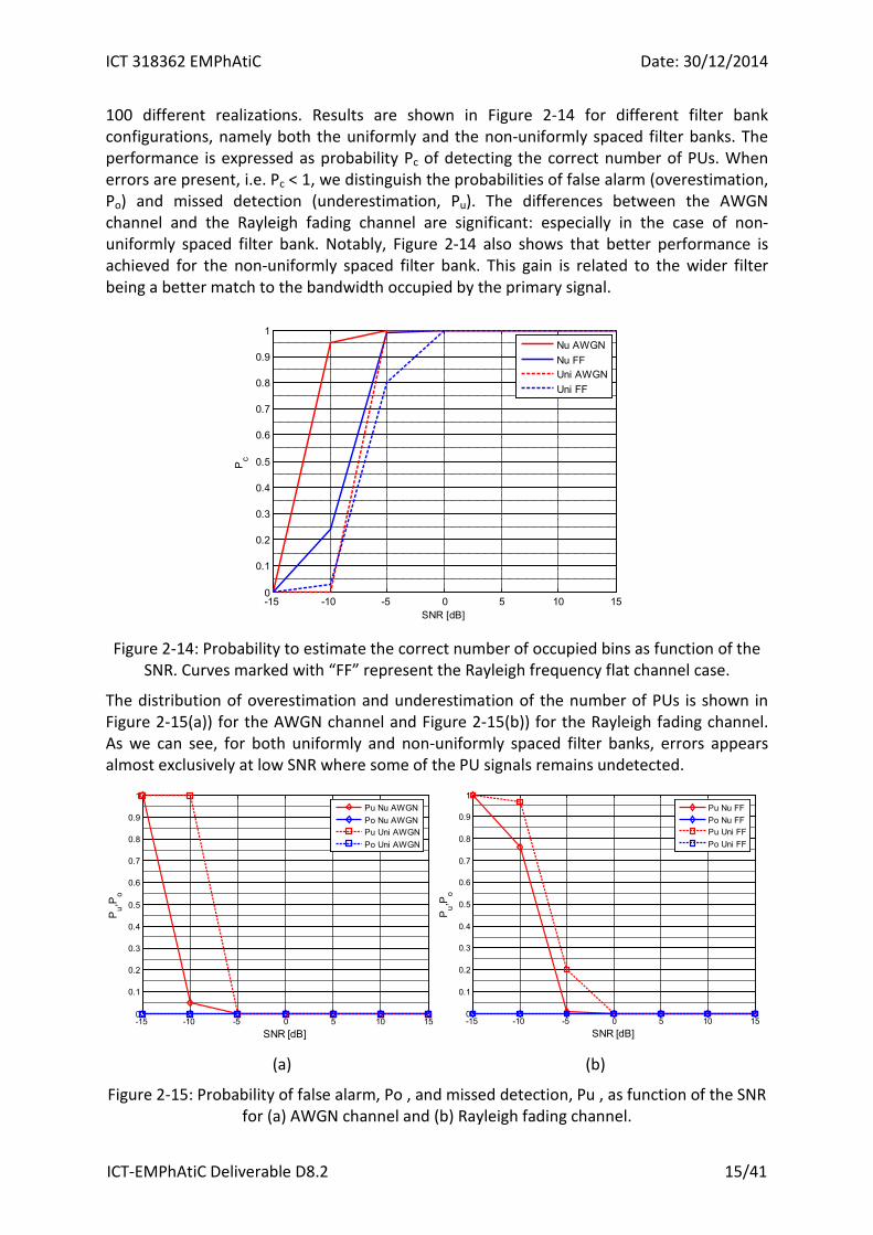
100 different realizations. Results are shown in Figure 2-14 for different filter bank configurations, namely both the uniformly and the non-uniformly spaced filter banks. The performance is expressed as probability Pc of detecting the correct number of PUs. When errors are present, i.e. Pc < 1, we distinguish the probabilities of false alarm (overestimation, Po) and missed detection (underestimation, Pu). The differences between the AWGN channel and the Rayleigh fading channel are significant: especially in the case of non-uniformly spaced filter bank. Notably, Figure 2-14 also shows that better performance is achieved for the non-uniformly spaced filter bank. This gain is related to the wider filter being a better match to the bandwidth occupied by the primary signal.

Figure 2-14: Probability to estimate the correct number of occupied bins as function of the

SNR. Curves marked with “FF” represent the Rayleigh frequency flat channel case.

The distribution of overestimation and underestimation of the number of PUs is shown in Figure 2-15(a)) for the AWGN channel and Figure 2-15(b)) for the Rayleigh fading channel. As we can see, for both uniformly and non-uniformly spaced filter banks, errors appears almost exclusively at low SNR where some of the PU signals remains undetected.

(a) (b)

Figure 2-15: Probability of false alarm, Po , and missed detection, Pu , as function of the SNR for (a) AWGN channel and (b) Rayleigh fading channel.

-15 -10 -5 0 5 10 150

0.1

0.2

0.3

0.4

0.5

0.6

0.7

0.8

0.9

1

SNR [dB]

Pc

Nu AWGNNu FFUni AWGNUni FF

-15 -10 -5 0 5 10 150

0.1

0.2

0.3

0.4

0.5

0.6

0.7

0.8

0.9

1

SNR [dB]

Pu,P

o

Pu Nu AWGNPo Nu AWGNPu Uni AWGNPo Uni AWGN

-15 -10 -5 0 5 10 150

0.1

0.2

0.3

0.4

0.5

0.6

0.7

0.8

0.9

1

SNR [dB]

Pu,P

o

Pu Nu FFPo Nu FFPu Uni FFPo Uni FF



When we compare this results with results obtained by using Model Order Selection framework (which are presented in the deliverable D8.1), it can be seen that CS-BP framework provides significant improvement. This improvement is especially present in the range of low SNR and the shift between performance curves is approximately 5 dB in the case of the AWGN channel and 10 dB in the case of the Rayleigh fading channel, for both filter bank configurations.



3 Sparse candidate shape detection This chapter proposes a new technique for spectrum sensing in the context of Broadband Professional Mobile Radio (B-PMR). The method exposed in this chapter is not only able to determine whether a given frequency subband is occupied or not, but also is able to distinguish if the transmission in an occupied subband is carried out by a primary or a secondary user.

Since Filterbank Multicarrier (FBMC) modulations are the physical-layer choice for secondary users within the EMPhAtiC project and the transmitting technologies used by the primary users are known (TETRA/TEDS), feature-based techniques can be applied for the detection of the licensed and the unlicensed users. With this aim in mind, herein a novel method is proposed. The exposed technique, which is named sparse candidate correlation matching, is based on the comparison of the spectral shape of the received signal with the “a priori” known power spectral density of the primary and secondary users. To avoid the complete signal reconstruction, the occupied channels are directly extracted from the sample autocorrelation matrix.

This chapter is organized as follows. The following section provides a brief overview of sparse signal representation and sparse regularization. The proposed method for spectrum sensing in the PMR band is proposed in section 3.2. Finally, the last section evaluates the performance of the proposed technique by means of some numerical results.

3.1 Brief introduction to sparse signal representation and structured sparsity

Sparse representation of signals over redundant dictionaries is a hot topic that has attracted the interest of researchers in many fields in signal processing during the last decade. It seeks to approximate a target signal by a linear combination of few elementary signals extracted from a known collection. We will start describing the general framework. Let us focus on finite dimensional spaces ℝn or ℂn. The most basic problem in sparse representation is the reconstruction of a vector 𝛉 from an observation vector 𝐮 = 𝚿𝛉, being 𝚿 the so-called dictionary, a known matrix of size 𝑚 x 𝑛. This matrix is usually overcomplete, i.e. it has more columns than rows. Under the assumption that the unknown vector is sparse, i.e., it has few non-zero entries as compared to its dimension, the natural approach is to seek the maximally sparse approximation of the observed vector 𝐮. Formally, this can be expressed as

min𝛉‖𝛉‖0 𝑠. 𝑡. 𝐮 = 𝚿𝛉 (3.1)

where ‖∙‖0 denotes the 𝑙0-(quasi) norm, a counting function that returns the number of non-zero elements of its argument. It is worth noting that, without imposing a sparsity prior on 𝛉, the systems of equation 𝐮 = 𝚿𝛉 is underdetermined and admits an infinite number of solutions. This problem is an NP-hard combinatorial problem in general. Fortunately, over the past decade, researchers have developed mathematical tools for solving sparse approximation problems with computationally tractable algorithms. Among all the techniques, the use of convex norms and greedy methods has deserved special attention in the literature [3].



To circumvent the computational bottleneck of the combinatorial problem in (3.1), the most common approach is to replace the non-convex 𝑙0-norm by the convex 𝑙1-norm, which is defined as ‖𝛉‖1 = ∑ |θ𝑖|𝑖 . This approach leads to the following convex problem with a lower computational complexity:

min𝛉‖𝛉‖1 𝑠. 𝑡. 𝐮 = 𝚿𝛉 (3.2)

The conditions that guarantee the equivalence of the solutions of (3.2)and (3.1) were studied in [4] and [5].

If some noise is present in the observation, or 𝐮 can only be assumed to be approximated by a sparse vector, a natural variation is to relax the exact match between 𝐮 and 𝚿𝛉 to allow some error tolerance ε ≥ 0. This leads to the following optimization problem

min 𝛉‖𝛉‖1 𝑠. 𝑡. ‖𝐮 −𝚿𝛉‖22 ≤ ε (3.3)

which is normally replaced by the following equivalent penalized least squares problem min

𝛉 ‖𝐮 −𝚿𝛉‖22 + 𝜆 ‖𝛉‖1 𝑤𝑖𝑡ℎ 𝜆 ≥ 0 (3.4)

where 𝜆 is a parameter that controls the balance between the sparsity of the solution induced by the 𝑙1-norm and the data reconstruction error. This method is known as the LASSO in statistics and as Basis Pursuit Denoising (BPDN) in signal processing. The sparse approximation problems exposed above are based on the relaxation of the non-convex 𝑙0-norm by the 𝑙1-norm. Nevertheless, recent papers [7], [8] show that the performance of 𝑙1-norm minimization problems can be further improved by considering a weighted formulation of the 𝑙1-norm minimization. The key point of this approach is that the main difference between the 𝑙1-norm and the 𝑙0-norm is the dependence on the magnitude: in the 𝑙1-norm, large coefficients are penalized more heavily than smaller coefficients, unlike the more democratic penalization in the 𝑙0-norm. To address this imbalance, if some “a priori” knowledge about the problem is available, it can be used to design a weighted 𝑙1-norm that democratically penalizes nonzero entries. The weighted 𝑙1-norm minimization is formulated as follows

min 𝛉

‖𝐮 −𝚿𝛉‖22 + 𝜆 ‖𝐖𝛉‖1 𝑤𝑖𝑡ℎ 𝜆 ≥ 0 (3.5)

being 𝐖 = diag{𝑤1 ⋯ 𝑤𝑛} a diagonal matrix with positive weights. Note that ‖𝐖𝛉‖1 = ∑ 𝑤𝑖|θ𝑖|𝑖 .

In the problems described above, sparsity is treated by considering each variable individually. In other words, each variable is regarded independent of the others. Nevertheless, the estimation in many practical situations could potentially benefit from additional information about the dependencies between the sets of variables. This strategy, which is the so-called structured sparsity, has recently received much attention in the machine learning and the signal processing communities [6]. The most common approach is to exploit some prior knowledge about the structural dependences in the data by including an appropriate regularisation term which promotes sparsity over the sub-groups of variables. This prior information leads to more interpretable solutions and improves the predictive performance of the system. An exponent of the group of structured sparsity problems is the group LASSO regularization that is briefly described below.



Let us divide the set of 𝑛 entries of 𝛉 into 𝐺 non-overlapping groups denoted by {𝐼1, … , 𝐼𝐺} and let 𝛉𝑔 refer to the subset of variables of 𝛉 in the group 𝐼𝑔. To promote sparsity at group level rather than just sparsity in 𝛉, we need to consider the group LASSO criterion exposed in the next problem

min 𝐮

‖𝐮 −𝚿𝛉‖22 + 𝜆�𝑣𝑔𝑔

�𝛉𝑔�2 𝑤𝑖𝑡ℎ 𝜆 ≥ 0 (3.6)

where �𝑣𝑔�𝑔=1𝐺

denote the associated positive scalars acting as weights. Interestingly, the

penalty term in (3.6) promotes sparsity by deleting all the variables of a given group simultaneously.

3.2 Sparse candidate correlation matching The aim of this section is to describe the method proposed for spectrum sensing in the PMR band. The technique exposed in this section is based on the candidate spectrum detector proposed in [8]. The method described therein is a powerful technique to detect primary users in cognitive radios when the secondary users transmit with a bandwidth smaller than the primary ones. This approach is based on the fact that unlicensed users usually transmit at a rate lower than the primary ones in order not to disturb the quality of service of the licensed users. Unfortunately, this assumption does not hold in the scenarios under analysis within the EMPhAtiC project, in which unlicensed users using FBMC modulations can transmit with a bandwidth broader than the licenced ones. Therefore, in this section we extend the technique proposed in [8] to the scenario under analysis in this project.

3.2.1 Signal model Consider a received signal which is a sparse multiband signal composed by the superposition of one or several primary and secondary users. Let �𝜔1,𝑖�𝑖=1

𝑀and �𝜔2,𝑘�𝑘=1

𝑁denote the grid of

potential frequency locations of the primary and the secondary signals, respectively, in the explored PMR band. The received signal 𝑦(𝑡) can be expressed as

y(t) = �𝑥1(𝑡,𝑀

𝑖=1

𝜔1,𝑖) + �𝑥2(𝑡,𝑁

𝑘=1

𝜔2,𝑘) + 𝑛(𝑡),

where 𝑥1(𝑡,𝜔1,𝑖) denotes the analytical representation of the primary user signal corresponding to 𝜔1,𝑖, which is given by 𝑥1�𝑡,𝜔1,𝑖� = 𝑎1,𝑖𝑒𝑗𝑤1,𝑖𝑡. In the same way, 𝑥2(𝑡,𝜔2,𝑘) = 𝑎2,𝑘𝑒𝑗𝜔2,𝑘𝑡 denotes the analytical representation of a secondary signal corresponding to 𝜔2,𝑘. We assume that only few 𝑎1,𝑖 and 𝑎2,𝑘 are different from zero, those associated with the presence of a primary or secondary transmission, respectively. Similar to [8], for simplicity in the notation of model we have assumed linear propagation channels with no distortion. The robustness of the correlation matching method in front of frequency selective channels have been studied in [11] and the numerical results in the next subsection validate this robustness.

Without loss of generality, in the rest of this chapter we will assume that:

1) The waveforms transmitted by the primary users are 25-kHz TETRA signals.

2) Unlicensed users use the LTE-like FBMC frame structure described in Milestone 4 [9], in which the transmission takes place in groups of contiguous subcarriers. In particular, considering the LTE-like structure in [9], the subcarriers are



activated/deactivated in disjoint groups of 12 subcarriers spaced by 15 kHz, called resource blocks.

A possible matching between the 15-kHz-spaced FBMC subcarriers and the 25-kHz TETRA channels is shown in the following figure:

1 2 3 4 5 6 7

1 2 3 4 5 6 7 8 9 10 11 12

8

13

9

14 15

...

...

TETRA channels

FBMC subcarriers

Figure 3-1. Possible matching between 25-kHz space TETRA channels (top) and 15-kHz FBMC subcarriers (bottom)

Bearing in mind the assumptions above, for the purpose of the present work, it is important to stress that while the frequency scanning grid for the primary signal is built in terms of the TETRA channels, the analysis of the unlicensed occupancy is made at subcarrier level. In other words, �𝜔1,𝑖�𝑖=1

𝑀 correspond to the frequency channels which can be potentially

occupied by a TETRA user and �𝜔2,𝑘�𝑘=1𝑁

are the FBMC subcarriers which can be potentially occupied by a secondary user transmission.

The block diagram proposed for the cognitive radio receiver is shown in Figure 3-2.

Figure 3-2. Block diagram of the cognitive receiver

Below, we analyze this scheme.

3.2.2 Compressive sampling The cognitive receiver can take profit of the sparsity of the explored spectrum by applying sub-Nyquist sampling to reduce the sampling rate. Even though no methods have been proposed in the context of EMPhAtiC based on compressive sampling techniques for efficiently acquiring and reconstructing the samples in the analysis filterbank (AFB), the formulation proposed in the chapter is derived in terms of a known sampling matrix 𝚪 ∈ ℝ𝑃 x 𝑄 in order to allow the application of the proposed method in future sub-Nyquist-based AFB systems. Different choices of 𝚪 are available in the literature depending on the compressive sampling technique (see [10] for further information). The meaning of this matrix 𝚪 is described below.



In the compressive sampling framework the signal 𝑦(𝑡) is not sampled directly, but is passed through a set of properly designed analog filters {ℎ𝑚(𝑡)}𝑚=1

𝑃 and then sampled at a reduced rate 𝑓𝑠 ≤ 𝑓𝑁𝑦𝑞𝑢𝑖𝑠𝑡, yielding the compressive samples

𝑧[𝑚] = �ℎ𝑚(𝑡) ∗ 𝑦(𝑡)|𝑡=𝑚1

𝑓𝑠

where ∗ denotes the convolution. In order to determine the relationship between the Nyquist samples 𝑦[𝑛] = �𝑦(𝑡)|𝑡=𝑛𝑓𝑁𝑦𝑞𝑢𝑖𝑠𝑡−1 and the compressive samples 𝑧[𝑚], consider a

complete observation of compressive data samples consisting of 𝐿 blocks of 𝑃 non-uniform data samples noted as {𝐳𝑘}𝑘=1𝐿 , where each of these blocks spans a sensing time 𝑇𝐵 =𝑃/𝑓𝑁𝑦𝑞𝑢𝑖𝑠𝑡. In this time the traditional Nyquist sampling would yield Q samples of 𝑦(𝑡) given by

𝐲𝑘 = [ 𝑦(𝑡1𝑘�… 𝑦(𝑡𝑄𝑘)]𝑇 𝑓𝑜𝑟 𝑘 = 1, … , 𝐿

where 𝑡𝑖𝑘 = (𝑘𝑄 + 𝑖)/ 𝑓𝑁𝑦𝑞𝑢𝑖𝑠𝑡. Therefore, the relation between the Nyquist samples and the sub-Nyquist samples is given by

𝐳𝑘 = 𝚪𝐲𝑘

being 𝚪 ∈ ℝ𝑃 x 𝑄 the so-called compressive sampling matrix, a known matrix whose rows contain the digital representation of the sampling filters {ℎ𝑚(𝑡)}𝑚=1

𝑃 . For instance, for the multi-coset strategy described in [8], 𝚪 is given by the random selection of 𝑃 rows of the identity matrix 𝑰𝑄.

3.2.3 Sparse correlation matching The purpose of this section is to design a feature-based method for cognitive sensing in the PMR band able to:

1) Detect the frequency sub-bands occupied in the received signal.

2) Distinguish if the occupied sub-bands are occupied by primary or unlicensed users.

To accomplish these two objectives we need to compare the “a priori” known spectral shape of the licensed and the unlicensed users with the power spectral density of the received signal by shifting the reference spectrum of the primary/secondary signals over the set of all the potential channel positions. In the method proposed herein the computation of the power spectral density is avoided by means of a second-order-based detector which relies on a correlation matching criterion.

Following the scheme exposed in Figure 3-2, the sample correlation matrix 𝐑� ∈ ℂ𝑃 x 𝑃 needs to be computed after the sub-Nyquist sampling process and is given by

𝐑� =1𝐿�𝐳𝑘

𝐿

𝑘=1

𝐳𝑘𝐻 = 𝚪 �1𝐿�𝐲𝑘

𝐿

𝑘=1

𝐲𝑘𝐻� 𝚪𝐻 (3.7)

For the purpose of the present work, let us define the baseband candidate autocorrelation of the primary and the secondary users, denoted by 𝐑b,1 and 𝐑b,2, respectively. These two matrices correspond to the autocorrelation of the impulse response of the basic baseband filters associated to the technologies of the licensed and the unlicensed users (in this case, TETRA and FBMC), and mainly depend on the modulation pulses and the baud rate of each system.



In order to obtain the frequency location of each primary user, the baseband correlation 𝐑b,1 needs to be multiplied by a rank-one matrix formed by the steering frequency vector of the explored frequency 𝑤1,𝑖.

𝐑c,1�𝜔1,𝑖� = 𝐑b,1⨀[𝒆�𝜔1,𝑖�𝒆�𝜔1,𝑖�𝐻

] (3.8)

where ⨀ denotes the Hadamard product of two matrices and 𝒆�𝜔1,𝑖� = [1 𝑒𝑗𝜔1,𝑖 … 𝑒𝑗𝑄𝜔1,𝑖]𝑇 is the frequency steering vector. Depending on the application, the baseband correlation 𝐑b,1 can be obtained analytically or has to be estimated from noise free data. For the 25-kHz TETRA case, the modulation pulse is a root-raised-cosine and 𝐑b,1 can be constructed building a Toeplitz matrix with the 𝑄 most relevant samples of the raised-cosine pulse (see Section III.A of [11] for further information).

Similarly, the candidate autocorrelation matrix for the FBMC signals can be designed at subcarrier level and is given by

𝐑c,2�𝜔2,𝑖� = 𝐑b,2⨀[𝒆�𝜔2,𝑖�𝒆�𝜔2,𝑖�𝐻

] (3-9)

According to this notation, the sample correlation matrix defined in (3.7) is given by,

𝐑� = �α�𝜔1,𝑖�𝚪𝐑c,1�𝜔1,𝑖�𝚪𝐻𝑀

𝑖=1

+ �β�𝜔2,𝑘�𝚪𝐑c,2�𝜔2,𝑘�𝚪𝐻𝑁

𝑘=1

+ 𝐑n (3-10)

where 𝐑n represents the noise autocorrelation matrix, α�𝜔1,𝑖� is the power level of the primary user at the frequency 𝜔1,𝑖 and β�𝜔2,𝑘� is the power level of the FMBC signal at the subcarrier 𝑘.

This model can be rewritten into a sparse notation as follows

𝐫� = (𝚪⨂𝚪)𝐁1𝐒1𝐩1 + (𝚪⨂𝚪)𝐁2𝐒2𝐩2 + 𝐫n = 𝐀1𝐩1 + 𝐀2𝐩2 + 𝐫n (3.11)

where ⨂ denotes the Kronecker product of two matrices and 𝐫� = vec�𝐑�� , being vec(∙) the vectorization operator. The remaining terms in (3.11) are defined as:

• 𝐁1 contains the information of the baseband correlation of the primary signal and is given by 𝐁1 = diag �vec�𝐑b,1��. Similarly, 𝐁2 is defined as 𝐁2 = diag �vec�𝐑b,2��.

• 𝐒1 is the matrix which defines the frequency scanning grid for the primary users and is expressed as follows 𝐒1 = �𝐬�𝜔1,1� ⋯ 𝐬�𝜔1,𝑀��, where 𝐬�𝜔1,𝑖� =vec �𝒆�𝜔1,𝑖�𝒆�𝜔1,𝑖�

𝐻�. In the same way, 𝐒2 define the frequency grid for the

secondary signal at subcarrier level.

• 𝐫n = vec(𝐑n) .

• 𝐩1 = �𝑝1�𝜔1,1� ⋯ 𝑝1�𝜔1,𝑀��𝑇

is a sparse vector with non-zero entries at positions corresponding to the locations of the primary users and 𝐩2 =�𝑝2�𝜔2,1� ⋯ 𝑝2�𝜔2,𝑁��

𝑇 is the sparse vector associated with the set of potential

locations of secondary signals. Since the analysis of the secondary signals is carried out at subcarrier level, non-zero indices are those corresponding to the FBMC subcarriers occupied by secondary transmissions.



• 𝐀1 = (𝚪⨂𝚪)𝐁1𝐒1 is the overcomplete dictionary of candidates for the signals of the licensed users and 𝐀2 = (𝚪⨂𝚪)𝐁2𝐒2 is the dictionary of candidates for the secondary signals.

The sparse formulation in (3.11) begs for the use of a sparse reconstruction strategy. This strategy needs to be tailored to our particular problem.

To find the primary users, the authors of [11] propose the following weighted 𝑙1-norm minimization

min 𝐩1�𝜔1,𝑖�≥𝟎

‖𝐫� − 𝐀1𝐩1‖22 + 𝜆 ‖𝐖1𝐩1‖1

𝑠. 𝑡. 𝐑� −�𝑝1�𝜔1,𝑖�𝚪𝐑c,1�𝜔1,𝑖�𝚪𝐻 ≽ 0𝑀

𝑖=1

(3.12)

The semidefinite constraint in (3.12) enforces the residual correlation after removing the primary candidates to be positive semidefinite and the weighted 𝑙1-norm in the objective function of (3.12) is proposed to democratically penalize the active entries of 𝐩1. The weights of the diagonal matrix 𝐖1 = diag{𝑤1, … ,𝑤𝑀}, were derived in [13] and are given by the maximum eigenvalue of 𝐑�−1�𝚪𝐑c,1�𝜔1,𝑖�𝚪𝐻�, that is,

𝑤𝑖 = 𝜆𝑚𝑎𝑥 � 𝐑�−1�𝚪𝐑c,1�𝜔1,𝑖�𝚪𝐻�� (3.13)

and have a clear physical meaning: the inverse of 𝑤𝑖 is a coarse estimate of the primary user power at 𝜔1,𝑖 and is the maximum power that can be removed at the frequency scanning point 𝜔1,𝑖 that preserves the positive semidefiniteness of 𝐑� − ∑ 𝑝1�𝜔1,𝑖�𝚪𝐑c,1�𝜔1,𝑖�𝚪𝐻𝑀

𝑖=1 ≽ 0 [11]. The maximum eigenvalue can be obtained efficiently using fast numerical techniques such as the power iteration method [14].

The method proposed in (3.12) is based on the assumption that secondary users transmit with a bandwidth smaller than the primary ones. Nevertheless, this assumption is not fulfilled in the scenario described in section 3.2.1. Therefore, we need to accommodate the transmissions of the secondary users in the formulation exposed in (3.12). Since the transmission of unlicensed signals take place activating/deactivating disjoint groups of 12 subcarriers, the sparsity has to be enforced on groups of 12 subcarriers (at the resource block level). Consider the scheme in Figure 3-3 for a possible organization pattern of the (potentially used) resource blocks.

Figure 3-3. Scheme of the LTE-like organization of the resource blocks (the DC carrier is left

unused).



Let 𝒢 denote the set of potentially used resource blocks and let 𝐩2𝑔 denote the subset of variables of 𝐩2 in the group 𝑔. In order to accommodate the transmissions of the secondary users in the model exposed in (3.12), we propose the following minimization problem

min 𝐩1,𝐩2≥𝟎

‖𝐫� − 𝐀1𝐩1 − 𝐀2𝐩2‖22 + 𝜆 �‖𝐖1𝐩1‖1 + �𝑣𝑔𝑔∈𝒢

�𝐩2𝑔�2�

𝑠. 𝑡. 𝐑� −�𝑝1�𝜔1,𝑖�𝚪𝐑c,1�𝜔1,𝑖�𝚪𝐻 −�𝑝2�𝜔2,𝑘�𝚪𝐑c,2�𝜔2,𝑘�𝚪𝐻𝑁

𝑘=1

≽ 0𝑀

𝑖=1

(3.14)

where the penalty term ∑ 𝑣𝑔𝑔 �𝐩2𝑔�2

is often referred to as a mixed-norm

regulariser [15], �𝐩2𝑔�2 stands for the Euclidean norm of the group 𝑔, i.e. 𝐩2𝑔, and 𝑣𝑔 are

the positive weights corresponding to the features in the 𝑔-group. Later we will address how these weights can be computed. The formulation presented in (3.14) seeks the linear combination of primary and secondary signals that best fits the sample autocorrelation matrix, subject to a constraint on the positive semidefinite nature of the residual correlation 𝐑n in (3-10). Note that the sparsity in the vector of primary powers 𝐩1 is enforced by means of a weighted 𝑙1-norm and group sparsity is promoted at resource block level (in groups of 12 subcarriers) in the vector 𝐩2. Following an idea similar to the one exposed for the computation of 𝐖1 [c.f. (3.13)], the weights 𝑣𝑔 in (3.14) can be obtained as

𝑣𝑔 = max 𝑖∈𝑔

�𝜆𝑚𝑎𝑥 � 𝐑�−1�𝚪𝐑c,2�𝜔2,𝑖�𝚪𝐻�� (3-15)

3.3 Simulation results The performance of the correlation matching method exposed above is analysed in this section. To carry out this objective, some simulations have been done following the guidelines in [9]. The signal to sense contains the contribution of a primary and a secondary user and has been critically sampled at 1.92 MHz. The primary signal is a 25 kHz TETRA signal and the FBMC signal transmitted by the SU has been generated using a 15-kHz-spaced FBMC/OQAM modulator of 128 subcarriers. The prototype pulse considered for the unlicensed modulation is the one proposed by the PHYDIAS project [16], with an overlapping factor 𝜅 = 4. Figure 3-1 presents the matching between the 15-kHz-spaced FBMC subcarriers and the 25-kHz TETRA channels. To start with, we have considered a received signal which is the superposition of a SU signal occupying the resource blocks 1 and 10 in the scheme shown in Figure 3-3 and a primary signal occupying the TETRA channel number 20. The channel between the PU and the cognitive receiver is modelled according to the Extended Pedestrian A (EPA) model exposed in [15] and the channel considered for the impinging secondary signal is an Extended Vehicular A (EVA). Both signals are received with the same power 𝑃𝑠 and contaminated with a Gaussian noise of variance 𝜎2 which affects the sensing band of 1.92 MHz. First, the performance of the proposed method will be analysed without considering compressive sampling. Thus, the sampling matrix 𝚪 is directly given by 𝚪 = 𝐈𝑄. Throughout all the



experiments exposed below, the sample correlation matrix of size 𝑄 = 64 is computed from a received data record of a length equivalent to 400 FBMC symbols (26 ms) and the convex optimization problem presented in (3.14) is solved using CVX, a MATLAB package for disciplined convex programming [18]. In order to illustrate the ability of the correlation matching method to distinguish between a primary and a secondary signal, Figure 3-4 and Figure 3-5 show the average performance of the proposed method after 100 Monte Carlo runs for 𝑃𝑠

𝜎2= −5 dB. Figure 3-4 shows the

estimated vector of powers for the secondary bands 𝐩2. This vector has a length of 120 subcarriers which correspond to the 10 resource blocks exposed in Figure 3-3. Note the TETRA signal, which affects the subcarriers 32-34, is almost rejected. In the same way, Figure 3-5 shows the estimated power in the grid of TETRA channels. See that the effect of the FBMC in the primary grid is almost negligible.

Figure 3-4. Estimated vector 𝐩2 versus the potentially occupied subcarriers (10 resource

blocks x 12 subcarriers)

Figure 3-5. Estimated vector 𝐩1 versus the potentially occupied TETRA channels



Now we want to analyse the detection capabilities of the correlation matching algorithm. As it has been already exposed in [8], the theoretical derivation of a detection threshold to meet a required false alarm probability is a difficult task. Following the approach considered in [8], to find an approximate derivation of the thresholds, we have recorded 500 Monte Carlo simulations for different values of 𝑃𝑠

𝜎2 and we have examined the probability of

detection and the probability of false alarm.

Figure 3-6 shows the ROC curves for the detection of a primary user for different values of 𝑃𝑠𝜎2

. Note that the performance of the method is highly degraded at 𝑃𝑠𝜎2

≤ −26 dB. It is worth noting that since the noise is uniformly distributed in the whole frequency band of 1.92 MHz and the primary signal only occupies 25 kHz, the ratio 𝑃𝑠

𝜎2 is not the SNR. Actually,

a 𝑃𝑠𝜎2

= −26 dB is approximately equivalent to a SNR of −6 dB in the 25-kHz TETRA subband under analysis.

Figure 3-6. ROC curves for the primary user for different values of 𝑃𝑠𝜎2

A similar procedure has been considered for the detection of a secondary user. In this case, a resource block is considered occupied if the mean of the estimated powers for the secondary signal exceeds the threshold. Figure 3-7 shows the corresponding ROC curves. Note that the performance of the correlation matching method is highly degraded for values of 𝑃𝑠

𝜎2 lower than −13 dB (around −5 dB of SNR for a secondary transmission occupying 2

resource blocks).



Figure 3-7. ROC curves for the detection of a secondary signal for different values of 𝑃𝑠𝜎2

Next, we analyse the degradation of the performance capabilities of the proposed method when compressive sampling is considered. Figure 3-8 and Figure 3-9 show the ROC curves for the detection of the primary and the secondary users for 𝑃𝑠

𝜎2= −18 dB and = −7 dB,

respectively, as a function of the compression rate 𝜌 = 𝑃𝑄

. Note that in both figures, the degradation in the performance of the detectors is small. In agreement with the Landau’s lower bound, the performance of the both detectors remains stable because the compression rate does not exceed the spectral occupancy.

Figure 3-8. ROC curves for the detection of a primary signal as a function of different

compression rates when 𝑃𝑠𝜎2

= −18 dB



Figure 3-9. ROC curves for the detection of a secondary signal as a function of different

compression rates when 𝑃𝑠𝜎2

= −7 dB



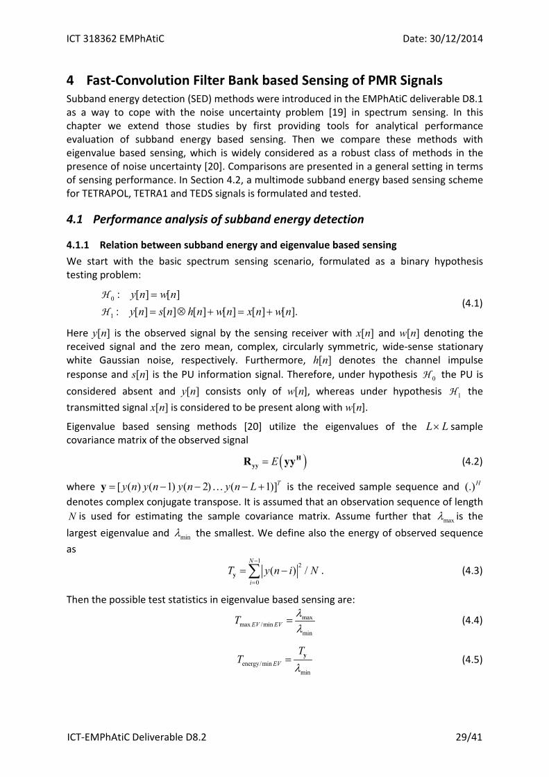
4 Fast-Convolution Filter Bank based Sensing of PMR Signals Subband energy detection (SED) methods were introduced in the EMPhAtiC deliverable D8.1 as a way to cope with the noise uncertainty problem [19] in spectrum sensing. In this chapter we extend those studies by first providing tools for analytical performance evaluation of subband energy based sensing. Then we compare these methods with eigenvalue based sensing, which is widely considered as a robust class of methods in the presence of noise uncertainty [20]. Comparisons are presented in a general setting in terms of sensing performance. In Section 4.2, a multimode subband energy based sensing scheme for TETRAPOL, TETRA1 and TEDS signals is formulated and tested.

4.1 Performance analysis of subband energy detection

4.1.1 Relation between subband energy and eigenvalue based sensing We start with the basic spectrum sensing scenario, formulated as a binary hypothesis testing problem:

0

1

: [ ] [ ]: [ ] [ ] [ ] [ ] [ ] [ ].

y n w ny n s n h n w n x n w n

== ⊗ + = +

H

H (4.1)

Here y[n] is the observed signal by the sensing receiver with x[n] and w[n] denoting the received signal and the zero mean, complex, circularly symmetric, wide-sense stationary white Gaussian noise, respectively. Furthermore, h[n] denotes the channel impulse response and s[n] is the PU information signal. Therefore, under hypothesis 0H the PU is considered absent and y[n] consists only of w[n], whereas under hypothesis 1H the transmitted signal x[n] is considered to be present along with w[n].

Eigenvalue based sensing methods [20] utilize the eigenvalues of the L L× sample covariance matrix of the observed signal

( )E= HyyR yy (4.2)

where [ ( ) ( 1) ( 2) ( 1)]Ty n y n y n y n L= − − − +y is the received sample sequence and (.)H denotes complex conjugate transpose. It is assumed that an observation sequence of length N is used for estimating the sample covariance matrix. Assume further that maxλ is the largest eigenvalue and minλ the smallest. We define also the energy of observed sequence as

1

2

0( ) /

N

iT y n i N

−

=

= −∑y . (4.3)

Then the possible test statistics in eigenvalue based sensing are:

maxmax /min

minEV EVT λ

λ= (4.4)

energy/minmin

EV

TT

λ= y (4.5)



maxmaxEV/energyT

Tλ

=y

(4.6)

The two first ones are more commonly considered in the literature [20], while the third one has been shown to have reduced computational complexity when effective power iteration method is used for calculating the maximum eigenvalue [21].

It is well established in the literature that the eigenvalue spread of the sample covariance matrix is related to the variations of the power spectral density (PSD) of the observed signal [22][23]. For white noise, the eigenvalues are approximately the same and the PSD is flat. Specifically, the eigenvalue ratio is bounded by the ratio of the maximum and minimum of the PSD function ( )S f :

max max

min min

SS

λλ

≤ (4.7)

4.1.2 Subband energy based sensing In subband energy detection (SED) [24][25], the idea is to use FFT or analysis filter bank (AFB) to split the observed signal into a number of ( M ) relatively narrow subbands and calculate the subband energies as

1

2

0( ) /

SBN

k k SBl

T y l N−

=

= ∑ (4.8)

where SBN is the number of subband samples during the observation interval. Commonly critically sampled subband signals are used in FFT-based SED, while 2x oversampled subband signals may be used in AFB based SED. In the analysis we assume critical sampling and /SBN N M= . Depending on the subband frequency response, some benefit may be obtained in the AFB case due to subband oversampling [26].

The test statistic is based on the maximum and minimum of the subband energies. Based on Eq. (1.6), a natural choice for the test statistic would be the ratio of the maximum and minimum subband energies:

{ }{ }max/min

maxmin

kSED

k

TT

T= . (4.9)

An alternative test statistic is the difference of maximum and minimum subband energies:

{ } { }max min max minSED k kT T T− = − . (4.10)

Actually, the latter test statistic is easier to treat analytically, and it will be seen to provide slightly better performance.

In all considered cases, the test statistic is compared to a predetermined threshold which is calculated based on the sample complexity and target false alarm probability. If the threshold is exceeded, a PU is deemed to be present in the observed frequency band, otherwise the band is considered to be available for secondary transmission.

In case of max-min-SED, the analysis is based on the Gumbel probability distribution [27]. Under H0 hypothesis,



0

2 2 2, , ,

max min6 6| ~ ,

2 SB

w k w k w kSED

SB

TN N

Cσ σ σ

π π−

+

H G (4.11)

where ( , )α βG denotes the Gumbel distribution and α and β are the location and scale parameters of the distribution, respectively. The standard Gumbel complementary

distribution function is given by ( ) 1x

ex eαβα

β

−−

−−= −G [27]. In (4.11) 2

,w kσ is the subband

noise variance (assumed to be Gaussian and the same for all subbands) and 0.5772C = is the Euler’s constant. The noise uncertainty (NU) is commonly expressed by the parameter ρ such that the actual noise variance is in the range 2 2 2

, , ,[(1/ ) , ]w k n k n kσ ρ σ ρσ= where 2,n kσ is the assumed value of

the subband noise variance. Then the worst-case false alarm probability can be expressed as:

2 2 2, , ,

2 2 2 2, , , ,

1/4 1/41 , ,,

6 62 2

max6 6w k n k n k

SB SB

SB S

w k w k n k n k

FA

w kk

Bn

CN N

N

P

N

C

σ σ ρσρ

σ σ ρσ ρσγ γ

π π

σ ρσππ

∈

− + − +

= =

G G . (4.12)

Based on this expression, the decision threshold can be expressed as:

1/4 2 2

, ,1,

6 6( ) .2SB SB

n k n kFA n kN N

P Cρσ ρσργ σ

π π−

= + +

G (4.13)

Under H1 hypothesis,

1max min

6 6| ~ ,2SE

SD

B SB

CTN N

κ κ κπ π−

+

H G . (4.14)

Here 2max min ,w kE Eκ σ= − + , ( )2

max max k kkE H E= , ( )2

min min k kkE H E= , kH is the PU

channel gain in subband k, and kE is PU signal energy in subband k. For tractability of the statistical model, the PU subband energies are assumed to be constant and independent of the transmitted symbol sequence. Then the worst case probability of detection with NU can be expressed as:

2 2 2

, , ,

1/4 1/41 ,

ˆ ˆ6 62 2

minˆ6 6w k n k n k

SB SB

B

D

SB S

CN

N N

CN

Pσ σ ρσ

ρ

κ κ κ κγ γπ π

κ κπ π

∈

− + − +

= =

G G (4.15)

where 2max min ,ˆ /n kE Eκ σ ρ= − + .

4.1.3 Simulation results Both eigenvalue based and subband energy based sensing methods exploit the frequency selectivity of the observed PU signal. Frequency selectivity may be due to a frequency selective channel or due to the spectral shape of the transmitted signal, or both. In case of



highly frequency-selective channel from the PU transmitter to the sensing receiver, the channel effect may be sufficient for sensing. However, a more robust sensing performance can be reached if the sensed frequency band includes part of the passband and at least one of the transition bands and part of the stopband.

Before applying the above ideas in the PMR application, they are first tested and compared in a generic broadband sensing scenario, with 20 MHz PU bandwidth and 2x oversampling, i.e., the sensing band has a width of two times the PU signal bandwidth. QPSK or OFDM waveforms are considered for the PU, using ITU-R Vehicular A and typical indoor channel models [28]. The sample complexity (observation length) is 10240 high-rate samples. In subband energy based sensing, we use here just FFT for subband decomposition. The number of subbands is 8 or 32, which illustrate well the achievable performance in the considered scenario. In case of eigenvalue based sensing, the dimension of the sample covariance matrix is 32x32. Both classes of methods are evaluated in the presence of 1 dB NU. As reference, energy detectors without NU, and with 0.1 dB and 1 dB NU are included.

First, Figure 4-1 compares eigenvalue based and subband energy based sensing methods in case of ITU-R Vehicular A channel. It can be seen that eigenvalue based and subband energy based methods provide rather similar sensing performance and exhibit high robustness against noise uncertainty. Also, the performance with QPSK and OFDM primaries is rather similar. Figure 4-2 compares analytical and simulated performance of max-min-SED under the indoor channel model, indicating rather good match. Figure 4-3 shows a ROC plot highlighting the robustness of max-min-SED against noise uncertainty. Finally, Figure 4-4 compares different subband energy based detection methods. The differential max-min-ED has been presented earlier in [24]. However, our conclusion is that the presented, conceptually much simpler max-min-SED method provides systematically somewhat better performance and higher robustness in different scenarios [25][29]. Also max/min-SED is included in the comparison, and it is found to have slightly lower performance than max-min-SED.

Figure 4-1. Detection probabilities using eigenvalue based detectors and max-min-SED with

ITU-R Vehicular A channel, 2x-oversampling, and N=10240. ‘EMaxE’ refers to the max EV/energy method. Upper: QPSK PU signal. Lower: OFDM PU signal



Figure 4-2. Analytical and simulated detection probabilities for QPSK PU signal under Indoor

channel with 2x-oversampling and N=10240

Figure 4-3. Receiver Operating Characteristics for the max-min-SED and the traditional ED

with OFDM PU signal with -14 dB SNR under Indoor channel, 2x-oversampling, and N=10240



Figure 4-4. Simulated detection probabilities for different subband energy based detectors for QPSK PU signal under Indoor channel with N=10240.

Upper: Without oversampling. Lower: 2x-oversampling

4.2 Joint sensing of TERAPOL, TETRA, and TEDS waveforms In this subsection we consider spectrum sensing in the following scenario:

• Sensing bandwidth of 180 kHz, corresponding to one resource block of 12 subcarriers.

• The sensed band may contain one or several primaries with 12.5 kHz TETRAPOL signal, 25 kHz TETRA1 signal, or 50 kHz TEDS signal, or mixture of those.

• The primary target is to test whether or not the band is free of any primary transmissions.

• Initially, no knowledge about the used channel raster is assumed, i.e., the potential primaries may have any center frequency within the sensing band. Later, also the gains due to availability of such knowledge are discussed.

• Fast-convolution filter bank (FC-FB) is used for sensing, utilizing the subband energy detection ideas presented above and in Deliverable D8.1.

In D8.1, it was concluded that it is advantageous to design the sensing filter frequency response independently of the FC-FB weight design used for data transmission. Raised-Cosine (RC) type frequency responses were utilized instead of Root-Raised-Cosine (RRC) type to minimize spectrum leakage from frequencies outside the sensing band.

In the considered multimode sensing scenario, one challenge is to design a common filter type for the three different PU signal types. Perhaps the most important issue is that the filter bandwidth is small enough for the most narrowband case, the 12.5 kHz TERAPOL signal. If the filter noise bandwidth is significantly wider than the signal bandwidth, the sensing performance is degraded.

Another important issue is the spacing of the subbands of the sensing filter bank. If the spacing is too high, it may happen that none of the subbands covers well-enough an



arbitrarily placed TETRAPOL channel. On the other hand, increasing the number of subbands degrades somewhat the performance of max-min-SED. It should be noted already in this context that if there is knowledge about the potential center frequencies of the primaries (channel raster), the design for optimized sensing performance becomes easier.

We assume that the main parameters of the FC-FB are the same as in the EMPhAtiC demonstrator: 1.4 MHz LTE-like case, transmission bandwidth corresponding to 72 active subcarriers of 15 kHz. Long transform (FFT) size N=1024, and overlap factor = 6/16. The 30 kHz subcarrier width for FBMC/OQAM modulation corresponds to 16 FFT bins, resulting in the IFFT size of 16. However, when considering raised cosine (RC) type filter for sensing, it is found to be feasible to use IFFT length of 8, i.e., 15 kHz total bandwidth and about 6 kHz 3 dB-bandwidth, resulting in RC spectrum which fairly well matches with the spectrum of a TETRAPOL signal. The FFT weights and interference leakage characteristics of such a design are shown in Figure 4-6. The interference leakage performance is found to exceed that of the data transmission filter, even with complex weights. We use 3.75 kHz spacing of sensing subbands, which means that 48 subbands are needed to cover the 180 kHz sensing band.

We tested subband energy based sensing algorithms of TETRAPOL, TETRA1, and TEDS signals using sensing duration of 53.33 ms, which corresponds to 800 subband samples with 2x oversampling. The SNRs are calculated using the nominal bandwidths of different waveforms (12.5/25/50 kHz) as the noise bandwidths. The results are shown in Figure 4-6. Targeting at 0.1FAP = and 0.99DP = , about -8 dB SNR is reached for TEDS and -7.5 dB SNR for TETRA1 and TETRAPOL when using the max-min-SED approach. For TETRAPOL, also the case with worst-case frequency offset of the PU channel (half of the sensing subband spacing) is shown. Clear (about 0.5 dB) loss in sensitivity is observed, which means the use of as many as 48 subbands is justified. For the TETRA1 and TEDS cases, such frequency offsets do not essentially affect the performance. It is also seen that max/min-SED is systematically slightly worse than max-min-SED. The third sensing method, max-SED, is based on searching the maximum subband energy and making the decision based on the basic energy detection approach, assuming knowledge of noise variance. With perfect knowledge of noise variance, this method is clearly better than the other ones. However, even 0.1 dB noise uncertainty significantly degrades the performance. On the other hand, both max-min-SED and max/min-SED are robust to noise uncertainty.

Figure 4-5. Characteristics of optimized RRC-type FBMC/OQAM subchannel filter (complex

weights) and RC-type sensing filter (real weights). Left: FFT-domain weight masks. Right: Interference leakage from a strong sinusoid.

-15 -10 -5 0 5 10 150

0.1

0.2

0.3

0.4

0.5

0.6

0.7

0.8

0.9

1

Frequency [kHz]

Mag

nitu

de

-100 -50 0 50 100 150 200

-100

-80

-60

-40

-20

0

Frequency [kHz]

Inte

rfere

nce

leve

l [dB

c]

FBMC/OQAM subchannel filterSensing filter



Figure 4-6. ROC-plots for TETRAPOL (12.5 kHz), TETRA1 (25 kHz), and TEDS (50 kHz) in joint

subband energy based sensing.

In the above study, it was assumed that the PU center frequencies may be arbitrary within the sensing band. If the possible center frequencies are known, then the number of subbands can be reduced, which reduces complexity and improves the performance somewhat. Generally, the TETRA channel raster has the spacing of 6.25 kHz. This already helps to reduce the number of subbands from 48 to 29. Further, if the potential TETRAPOL, TETRA1 and TEDS channel center frequencies are known and they are spaced at 12.5, 25, and 50 kHz, respectively, the number of subbands can be reduced to 15, 8, or 4, respectively, while sensing each of these specific waveforms.

If the targeted minimum SNR for PU detection is the same for all signal bandwidths, then the lowest bandwidth case determines the needed sensing duration. Using the same narrowband filter for different PU types, the sensitivity is slightly improved for wider bandwidths, as can be seen in Figure 4-6. Further optimization of the sensing process would anyway help to detect PUs with wider bandwidth more quickly and this would also reduce the signal processing and energy spent on sensing in those cases.

For the wider bandwidth PU cases, using wider bandwidth for the sensing filter helps to reduce the required sensing duration. If there is knowledge that only TETRA and/or TEDS signals are present in the band, then wider bandwidth should be used for the sensing filter, resulting in significant reduction in the sensing duration. This can be done also by integrating subband energies obtained from narrow subband filters. Assume that first the subband energies are first computed using a time record length of SBN subcarrier samples

10-3

10-2

10-1

100

10-4

10-3

10-2

10-1

100

PFA

PM

D

TETRAPOL, SNR=-7.5 dB, no offset

max/min SEDmax-min SEDmax SEDTarget PFA

0.1 dB NU range

10-3

10-2

10-1

100

10-4

10-3

10-2

10-1

100

PFA

PM

D

TETRAPOL, SNR=-7.5 dB, worst-case offset


0.1 dB NU range

10-3

10-2

10-1

100

10-4

10-3

10-2

10-1

100

PFA

PM

D

TETRA1, SNR=-7.5 dB, no offset


0.1 dB NU range

10-3

10-2

10-1

100

10-4

10-3

10-2

10-1

100

PFA

PM

D

TEDS, SNR=-8 dB, no offset


0.1 dB NU range



with narrowband sensing filter. Let kT be the test statistic for subband k. Then the test statistic for a PU with wider bandwidth is obtained by averaging the energies of B subbands:

/2 1( )

/2

1 k BB

k ii k B

T TB

+ −

= −

= ∑ . (4.16)

Using the FC-FB sensing filter designed for TETRAPOL, the optimum values for TETRA1 and TEDS were found to be 1 5TETRAB = and 11TEDSB = .

The required sensing durations for different SED based sensing schemes are reported in Table 1 for the two target PU SNR values of -5 dB and -7.5 dB. The Uniform narrow subbands case corresponds to the max-min SED of Figure 4-6. In the second case, the subband energy averaging idea is applied with the mentioned optimum values of 1TETRAB and TEDSB with 3.75 kHz spacing of the subband center frequencies. It can be noted that in this case, the subband energy averaging can be implemented effectively with the recursive moving average filtering model. In the third case, known PU channel center frequencies are assumed, and the number of subbands in the max-min SED process is reduced to 15, 8, and 4, for TETRAPOL, TETRA1, and TEDS, respectively. It can be seen that the subband energy averaging idea greatly helps to reduce the required sensing duration for TETRA1 and TEDS primaries with wider bandwidths. The knowledge of PU channel center frequencies helps, but the effect is relatively smaller.

Considering a multimode sensing scenario where the secondary user doesn’t have knowledge about the potential PU waveform, different sensing durations are needed for different PU waveforms if the target sensitivities are the same. A practical way is to run separate sensing processes for TETRAPOL, TETRA1, and TEDS utilizing the same subband energy calculations. Instead of sensing decisions based on fixed block lengths, the sequential detection model [30] helps to make the decision about a reappearing PU as quickly as possible, depending on the waveform characteristics and PU power level. For example, if multiple, noncontiguous subframe-long sensing gaps are utilized, as discussed in deliverable 8.1, the sequential detection decisions could be made after each sensing gap.

Sensing scheme SNR TETRAPOL 12.5 kHz

TETRA1 25 kHz

TEDS 50 kHz

Uniform narrow subbands - no channel raster knowledge - 3.75 kHz sensing subband spacing

-7.5 dB -5.0 dB

55.0 ms 20.0 ms

50.0 ms 17.0 ms

38.3 ms 12.3 ms

Optimal subband widths - no channel raster knowledge - 3.75 kHz sensing subband spacing

-7.5 dB -5.0 dB

55.0 ms 20.0 ms

35.7 ms 12.3 ms

20.0 ms 6.7 ms

Optimal subband widths - with channel raster knowledge - 12.5/25/50 kHz sensing subband spacing

-7.5 dB -5.0 dB

45.3 ms 16.0 ms

32.7 ms 11.3 ms

18.0 ms 6.3 ms

Table 1: Comparison of required sensing durations in different max/min SED scenarios for -5 dB and -7.5 dB PU SNR’s, 0.1FAP = and 0.99DP = . Worst-case frequency offset of the PU

center frequency with respect to the sensing subbands is assumed in all cases.



5 Conclusions This deliverable describes the results of the work performed during task 8.1 "Application of Compressed sampling techniques", containing the results on computationally affordable algorithms that exploit the sparsity of the wide–band spectral, as well as analysis on developed computationally affordable adaptive algorithms that exploit spectral sparsity patterns in wide–band sensing and CR. It consists of three proposed methods focusing on a) the effectiveness of belief propagation framework for spectrum sensing in FBMC-based transmission systems, b) a novel feature-based technique for spectrum sensing in the context of Broadband Professional Mobile Radio (B-PMR), and c) subband energy detection based methods for robust spectrum sensing of the legacy PMR signals of the TETRA family.

Clearly, to be able to ensure a predictable and acceptable performance for a cognitive PMR network operating in licensed bands, most robust protocols require the knowledge of prior context variables (noise distribution, channel gain, probability of malicious users,…) [31]. More research is required to create a cognitive radio network that can really learn from the environment and improve its sensing accordingly to cope with all the peculiarities and security attacks that threaten the network.



6 References [1] Alexis Lamiable, Joanna Tomasik, "Validation of spectrum management schemes for PMR

networks based on LTE with interference detection", in Proc. Wireless Days 2013, 2013.

[2] Baron, D.; Sarvotham, Shriram; Baraniuk, R.G., "Bayesian Compressive Sensing Via Belief Propagation," Signal Processing, IEEE Transactions on , vol.58, no.1, pp.269,280, Jan. 2010.

[3] M. Elad, “Sparse and redundant Representations: From Theory to Applications in Signal and Image Processing”, Springer 2011.

[4] D. L. Donoho, “For most large underdetermined systems of equations, the minimal l1-norm near-solution approximates the sparsest near-solution”, vol. 59, no.7, ppp. 907-934, 2006.

[5] E. J. Candes and T. Tao, “Near-optimal signal recovery from random projections: universal encoding strategies”, IEEE Trans. Inf. Theory, vol. 52, no. 12, pp. 5406-5425, 2006.

[6] F. Bach, R. Jenatton, J. Mairal, G. Obozinski, “Structured sparsity through convex optimization”, Statistical science, vol. 27, no. 4, 450-468, 2012.

[7] E. J. Candes, M. B. Wakin, S. P. Boyd, “Enhacing Sparsity by Reweighted l1 minimization”, J. Fourier Anal. Appl., vol. 14, no. 56.

[8] E. Lagunas, M. Najar, “Compressed spectrum sensing in the presence of interference: comparison of sparse recovery strategies”, in Proc. European Signal Processing Conference (EUSIPCO), 2014.

[9] V. Ringset et al. “Document Milestone 4: Definition and specification of requirements for physical layer implementation and channel model”, Project ICT-318362 EMPhAtiC, MS4, September 2013.

[10] E. J. Candes, M. B. Wakin, “An introduction to compressive sampling”, in IEEE Signal Proc. Magazine, vol. 25, no. 2, pages 21-30, 2008.

[11] E. Lagunas, “Compressive sensing based candidate detector and its application to spectrum sensing and through-the-wall spectrum sensing”, PhD, Universitat Politècnica de Catalunya, Spain 2014.

[12] I. Pérez-Neira, M. A. Lagunas, M. A. Rojas, “ Correlation Matching Approach for Spectrum Sensing in Open Spectrum Communications”, IEEE Trans. Signal Proc., Vol. 57, No. 12, Dec. 2009.

[13] E. Lagunas, M. Nájar, “Robust primary user identification using compressive sampling for cognitive radios”, In proc. International Conference on Acoustic, Speech and Signal Processing (ICASSP) 2014.

[14] Y. Saad, “Numerical methods for large eigenvalue problems”, Manchester University Press, 2011.

[15] P. Zhao, G. Rocha, B. Yu, “ Grouped and hierarchical model selection trough composite absolute penalties”, Annals of Statistics, 37(A): 3468-3497, 2011.

[16] 3rd Generation Partnership Project, “LTE; evolved universal terrestrial access (e-UTRA); base station (BS) radio transmission and reception”, ETSI, Tech. Spec. TS36.104 vv 11.4.0, release 11, 2013.

[17] Viholainen et al., “ Prototype filter and structure optimization”, Project PHYDIAS, ICT-211887, Deliverable D5.1, Jan. 2009.

[18] Michael Grant and Stephen Boyd. CVX: Matlab software for disciplined convex programming, version 2.0 beta. http://cvxr.com/cvx, September 2013.



[19] R. Tandra and A. Sahai, “SNR walls for signal detection,” IEEE J. Sel. Topics Signal Process., vol. 2, no. 1, pp. 4-17, Feb. 2008.

[20] Y. Zeng and Y. C. Liang, “Eigenvalue-based spectrum sensing algorithms for cognitive radio,” IEEE Trans. Commun., vol. 57, no. 6, pp. 1784-1793, June 2009.

[21] S. Dikmese, A. Gokceoglu, M. Valkama and M. Renfors, “Reduced complexity spectrum sensing based on maximum eigenvalue and energy,” in Proc. Tenth International Symposium on Wireless Communication Systems, (ISWCS’13, Ilmenau, Germany), 5 p., Aug. 2013.

[22] S. Haykin, Adaptive Filter Theory, Prentice Hall Information and Sciences Series, 1996.

[23] G. V. Vilar, R. L. Valcarce, and J. Sala, “Multiantenna spectrum sensing exploiting spectral a priori information,” IEEE Trans. Wireless Commun., vol. 10, no. 12, pp. 4345-4355, Dec. 2011.

[24] P. Cheraghi, Yi Ma, R. Tafazolli, and L. Zhengwei, “Cluster-based differential energy detection for spectrum sensing in multi-carrier systems,” IEEE Trans. Signal Process., vol. 60, no. 11, pp. 6450-6464, Dec. 2012.

[25] S. Dikmese, P. C. Sofotasios, M. Renfors and M. Valkama, “Max-Min energy based spectrum sensing under frequency selectivity for cognitive radio,” in Proc. CROWNCOM Conf. (Oulu, Finland), pp. 347-352, June 2014.

[26] S. Dikmese, T. Ihalainen and M. Renfors, “Analysis and optimization of energy detection for non-flat spectral characteristics,” Chapter 3 in M.-G. Di Benedetto and F. Bader (Eds.), Cognitive Communication and Cooperative HetNet Coexistence, Springer 2014.

[27] S. Coles, An Introduction to Statistical Modeling of Extreme Values, Springer, London, 2001.

[28] R. Jain, “Channel Models: A Tutorial,” WiMAX Forum AATG, Feb. 2007.

[29] S. Dikmese, P. C. Sofotasios, M. Renfors, and M. Valkama, “Reduced complexity subband energy based spectrum sensing under noise uncertainty and frequency-selective spectral characteristics,” submitted to IEEE Trans. Signal Processing, Dec. 2014.

[30] N. Kundargi and A. Tewfik, "Hierarchical sequential detection in the context of dynamic spectrum access for cognitive radios," in Proc. Int. Conf. Electronics, Circuits and Systems (ICECS 2007), pp. 514-517, Dec. 2007.

[31] H. Rifà-Pous, M. Jiménez Blasco, and C. Garrigues, "Review of Robust Cooperative Spectrum Sensing Techniques for Cognitive Radio Networks", Wireless Personal Communications, pages 1–24, 10.1007/s11277-011-0372-x, 2011.



Glossary and Definitions

Acronym Meaning

AFB Analysis Filterbank

AWGN Additive White Gaussian Noise

B-PMR Broadband Professional Mobile Radio

ED Energy Detector

FBMC Filterbank Multicarrier

FBMC/OQAM Filterbank Multicarrier with Offset QAM Subcarrier Modulation

FC-FB Fast-Convolution Filterbank

FFT Fast Fourier Transform

LTE Long-Term Evolution

NU Noise Uncertainty

OFDM Orthogonal Frequency-Division Multiplexing

PSD Power Spectral Density

PU Primary User

QPSK Quadrature Phase-Shift Keying

RC Raised Cosine

ROC Receiver Operating Characteristics

RRC square Root Raised Cosine

SNR Signal-to-Noise Ratio

SU Secondary User

TEDS TETRA Enhanced Data Service

TETRA TErrestrial Trunked RAdio

enhanced multicarrier techniques for professional ad-hoc ... · enhanced multicarrier techniques...

Documents