energy consumption trends of multi-unit residential ... · pdf fileenergy consumption trends...
TRANSCRIPT
Energy Consumption Trends of Multi-Unit Residential Buildings in the City of Toronto
Authors:
Clarissa Binkley, University of Toronto
Marianne Touchie, University of Toronto
Kim Pressnail, University of Toronto
ii
Executive Summary Multi-unit residential buildings (MURBs) represent the most significant component in the Toronto
residential building inventory. Over half (56%) of the dwellings in the City of Toronto consist of
apartment buildings. Thirty-nine percent of all Toronto dwellings are either mid-rise or high-rise
apartment building of five or more storeys. The combined electricity and natural gas consumption of
Toronto MURBs is responsible for 2.5M tonnes eCO2 emissions annually. Given the large number of
MURBs, determining an accurate benchmark of energy intensity and developing an understanding of
how to reduce energy use is an important step in reducing the greenhouse gas emissions associated
with this sector. In establishing benchmarks, a standardized process that categorizes buildings into
groups with similar potential for improvement in energy-efficiency is needed. This potential for energy-
efficiency can then be used to prioritize the energy retrofit needs for certain typologies and so, inform
policy makers.
This study builds upon a previous project conducted by the authors, which was funded by the Toronto
Atmospheric Fund (TAF) and is entitled “Meta-Analysis of Energy Consumption in Multi-Unit Residential
Buildings in the Greater Toronto Area” (the Meta-Analysis). The aim of this study is to address the data
limitations of the Meta-Analysis by examining a refined data set composed of 40 buildings with more
complete energy consumption and building characteristics data.
The 40 MURBs in the refined data set account for 1.9% of the mid and high-rise MURB population in
Toronto. The buildings had construction dates ranging from 1960 to 2003, had heights ranging from five
to 28 storeys, and had between 24 and 250 suites in each building. Overall, the distribution of building
height and age in the refined data set was comparable to the actual distribution of building height and
age of Toronto mid and high-rise MURBs with two exceptions. The data set did not contain any
buildings constructed prior to 1960 or any buildings taller than 28 storeys.
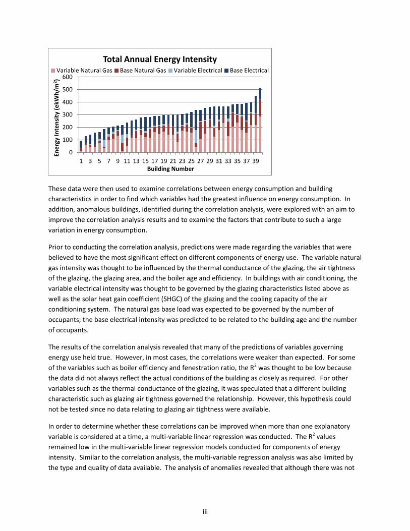
The weather-normalized total energy intensities ranged from 90ekWh/m2 to 510ekWh/m2 and averaged
292ekWh/m2. The energy intensities for the 40 buildings in this study, split up by variable natural gas
intensity, base natural gas intensity, variable electricity intensity and base electricity intensity, are
shown in the figure below.
iii
These data were then used to examine correlations between energy consumption and building
characteristics in order to find which variables had the greatest influence on energy consumption. In
addition, anomalous buildings, identified during the correlation analysis, were explored with an aim to
improve the correlation analysis results and to examine the factors that contribute to such a large
variation in energy consumption.
Prior to conducting the correlation analysis, predictions were made regarding the variables that were
believed to have the most significant effect on different components of energy use. The variable natural
gas intensity was thought to be influenced by the thermal conductance of the glazing, the air tightness
of the glazing, the glazing area, and the boiler age and efficiency. In buildings with air conditioning, the
variable electrical intensity was thought to be governed by the glazing characteristics listed above as
well as the solar heat gain coefficient (SHGC) of the glazing and the cooling capacity of the air
conditioning system. The natural gas base load was expected to be governed by the number of
occupants; the base electrical intensity was predicted to be related to the building age and the number
of occupants.
The results of the correlation analysis revealed that many of the predictions of variables governing
energy use held true. However, in most cases, the correlations were weaker than expected. For some
of the variables such as boiler efficiency and fenestration ratio, the R2 was thought to be low because
the data did not always reflect the actual conditions of the building as closely as required. For other
variables such as the thermal conductance of the glazing, it was speculated that a different building
characteristic such as glazing air tightness governed the relationship. However, this hypothesis could
not be tested since no data relating to glazing air tightness were available.
In order to determine whether these correlations can be improved when more than one explanatory
variable is considered at a time, a multi-variable linear regression was conducted. The R2 values
remained low in the multi-variable linear regression models conducted for components of energy
intensity. Similar to the correlation analysis, the multi-variable regression analysis was also limited by
the type and quality of data available. The analysis of anomalies revealed that although there was not
0
100
200
300
400
500
600
1 3 5 7 9 11 13 15 17 19 21 23 25 27 29 31 33 35 37 39
Ene
rgy
Inte
nsi
ty (
ekW
h/m
2)
Building Number
Total Annual Energy Intensity Variable Natural Gas Base Natural Gas Variable Electrical Base Electrical
iv
one particular factor that could explain a large group of the anomalies, information on the special
facilities included in the buildings aided in the explanation of a number of the anomalies.
The findings of this report indicate that heating system efficiencies and glazing characteristics, including
fenestration ratio in particular, as well as glazing U-value, are the variables that are most closely linked
to energy intensity. The lower-than-expected correlation coefficient between variable natural gas and
boiler efficiency could indicate that efficiency estimates of existing boilers are either not accurate or that
boiler efficiency does not inadequately describe the performance of the heating system as a whole. The
actual efficiency of the whole heating system should be assessed before retrofit decisions are
prioritized. Relatively strong correlations between fenestration ratio and variable natural gas intensity
were found. However, the fenestration ratio is a variable that cannot be easily altered in an existing
building. Thus, this finding could be used to influence design guidelines for new buildings in that lower
fenestration ratios should be encouraged. However, different coefficients in the correlation between
energy use and the fenestration ratio of single- and double-glazed units suggest that air-leakage may be
more prevalent in single-glazed windows. Though further investigation of the air tightness of various
existing window systems would be required to confirm this hypothesis, this finding could indicate the
importance of window air-sealing measures particularly in buildings with single-glazing. Additionally, the
estimated number of occupants in a building, obtained from census data, was found to be an important
variable influencing the base natural gas intensity. Census data were used because the actual number of
occupants was not readily available.
The analyses and conclusions from this study will be used to inform the next phase in this research
project. The next phase includes creating a database with the ability to add new buildings, generating
suggestions for typology-specific building upgrades and producing energy models of four buildings to
assess the effect of certain upgrades.

v
Acknowledgements The authors gratefully acknowlege the funding provided by the Toronto Atmospheric Fund and the
Hutcheon Bequest. A special thank you to Bryan Purcell for his thorough review and thoughtful
comments.
vi
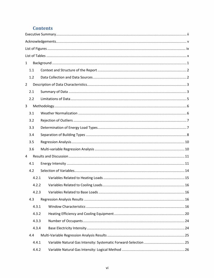
Contents Executive Summary ....................................................................................................................................... ii
Acknowledgements ....................................................................................................................................... v
List of Figures ............................................................................................................................................... ix
List of Tables ................................................................................................................................................. x
1 Background ........................................................................................................................................... 1
1.1 Context and Structure of the Report ............................................................................................ 2
1.2 Data Collection and Data Sources ................................................................................................. 2
2 Description of Data Characteristics....................................................................................................... 3
2.1 Summary of Data .......................................................................................................................... 3
2.2 Limitations of Data ........................................................................................................................ 5
3 Methodology ......................................................................................................................................... 6
3.1 Weather Normalization ................................................................................................................ 6
3.2 Rejection of Outliers ..................................................................................................................... 7
3.3 Determination of Energy Load Types ............................................................................................ 7
3.4 Separation of Building Types ........................................................................................................ 8
3.5 Regression Analysis ..................................................................................................................... 10
3.6 Multi-variable Regression Analysis ............................................................................................. 10
4 Results and Discussion ........................................................................................................................ 11
4.1 Energy Intensity .......................................................................................................................... 11
4.2 Selection of Variables .................................................................................................................. 14
4.2.1 Variables Related to Heating Loads .................................................................................... 15
4.2.2 Variables Related to Cooling Loads ..................................................................................... 16
4.2.3 Variables Related to Base Loads ......................................................................................... 16
4.3 Regression Analysis Results ........................................................................................................ 16
4.3.1 Window Characteristics ...................................................................................................... 16
4.3.2 Heating Efficiency and Cooling Equipment ......................................................................... 20
4.3.3 Number of Occupants ......................................................................................................... 24
4.3.4 Base Electricity Intensity ..................................................................................................... 24
4.4 Multi-Variable Regression Analysis Results ................................................................................ 25
4.4.1 Variable Natural Gas Intensity: Systematic Forward-Selection .......................................... 25
4.4.2 Variable Natural Gas Intensity: Logical Method ................................................................. 26
vii
4.4.3 Other Multi-Variable Regression Analyses ......................................................................... 26
5 Investigation of Anomalies ................................................................................................................. 28
5.1 Energy Intensity .......................................................................................................................... 29
5.2 Variable Natural Gas Intensity .................................................................................................... 30
5.3 Base Natural Gas Intensity .......................................................................................................... 31
5.4 Alternative Heating Systems ....................................................................................................... 32
5.5 Additional Facilities ..................................................................................................................... 32
6 Conclusions ......................................................................................................................................... 33
7 Recommendations .............................................................................................................................. 34
8 Next Phase of This Study ..................................................................................................................... 37
9 References .......................................................................................................................................... 38
10 Bibliography .................................................................................................................................... 39
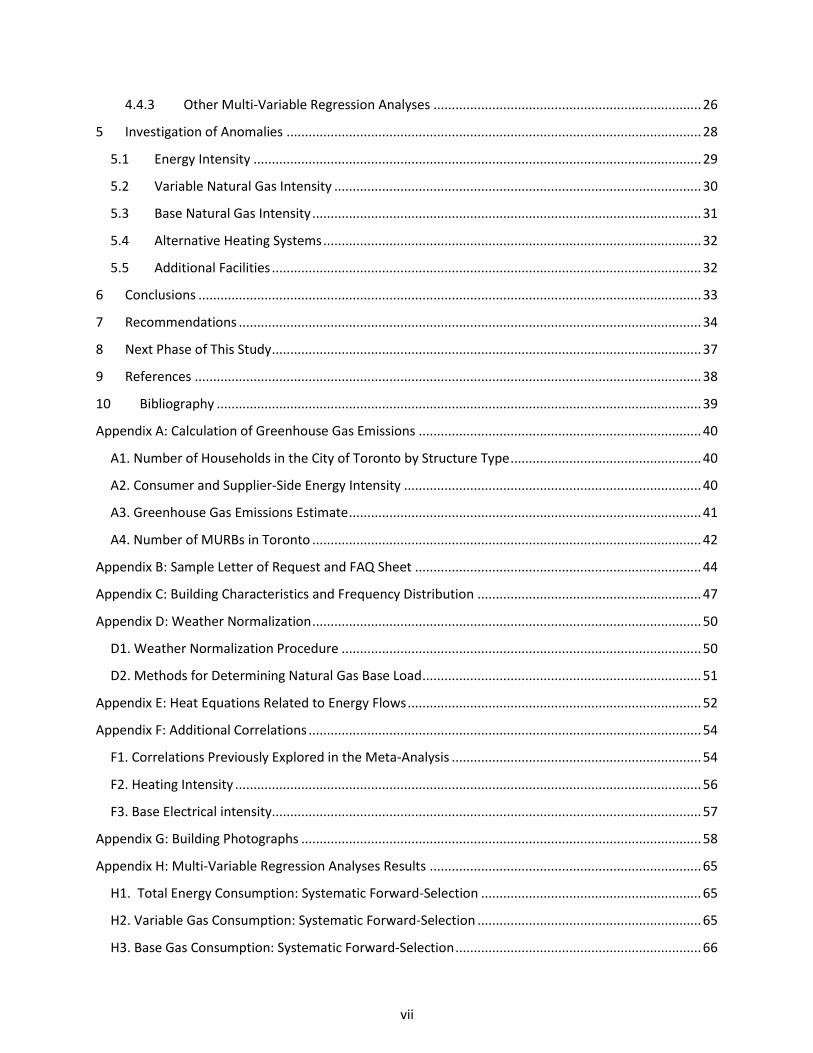
Appendix A: Calculation of Greenhouse Gas Emissions ............................................................................. 40
A1. Number of Households in the City of Toronto by Structure Type .................................................... 40
A2. Consumer and Supplier-Side Energy Intensity ................................................................................. 40
A3. Greenhouse Gas Emissions Estimate ................................................................................................ 41
A4. Number of MURBs in Toronto .......................................................................................................... 42
Appendix B: Sample Letter of Request and FAQ Sheet .............................................................................. 44
Appendix C: Building Characteristics and Frequency Distribution ............................................................. 47
Appendix D: Weather Normalization .......................................................................................................... 50
D1. Weather Normalization Procedure .................................................................................................. 50
D2. Methods for Determining Natural Gas Base Load ............................................................................ 51
Appendix E: Heat Equations Related to Energy Flows ................................................................................ 52
Appendix F: Additional Correlations ........................................................................................................... 54
F1. Correlations Previously Explored in the Meta-Analysis .................................................................... 54
F2. Heating Intensity ............................................................................................................................... 56
F3. Base Electrical intensity..................................................................................................................... 57
Appendix G: Building Photographs ............................................................................................................. 58
Appendix H: Multi-Variable Regression Analyses Results .......................................................................... 65
H1. Total Energy Consumption: Systematic Forward-Selection ............................................................ 65
H2. Variable Gas Consumption: Systematic Forward-Selection ............................................................. 65
H3. Base Gas Consumption: Systematic Forward-Selection ................................................................... 66

viii
H4. Variable Electricity Consumption: Systematic Forward-Selection ................................................... 66
H5. Base Electricity Consumption: Systematic Forward-Selection ......................................................... 66
H6. Total Energy Intensity: Systematic Forward-Selection .................................................................... 66
H7. Total Energy Intensity: Logical Method ........................................................................................... 67
ix
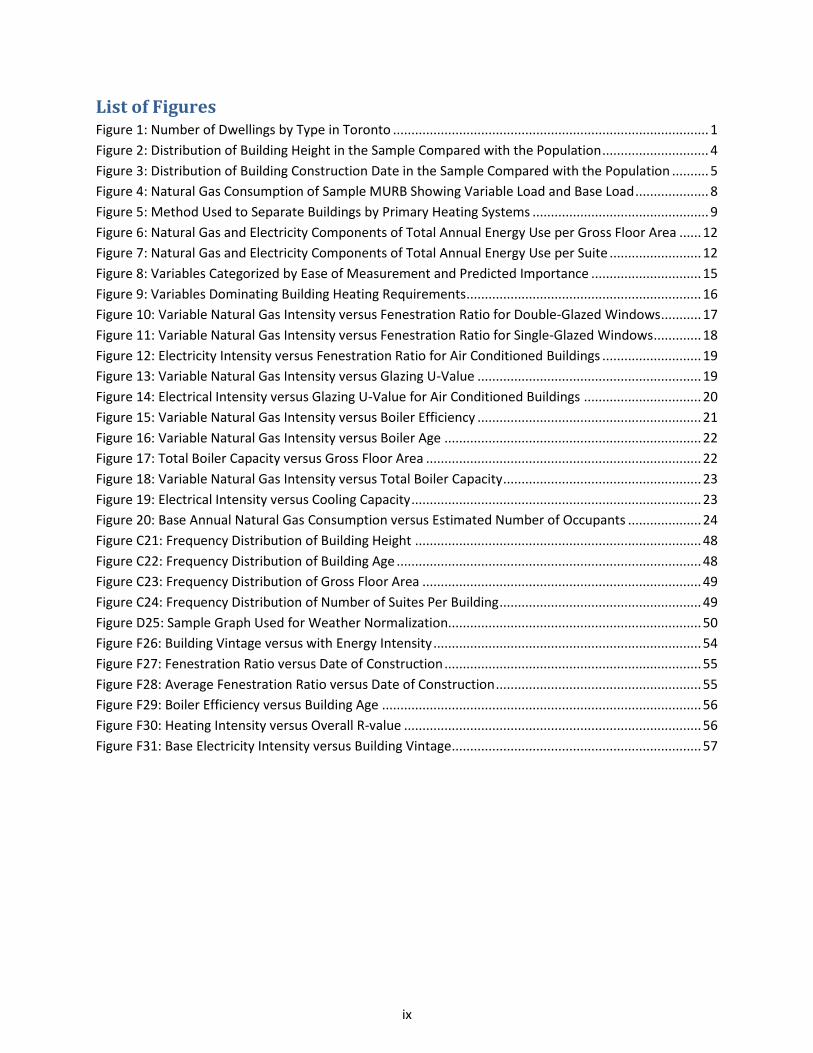
List of Figures Figure 1: Number of Dwellings by Type in Toronto ...................................................................................... 1
Figure 2: Distribution of Building Height in the Sample Compared with the Population ............................. 4
Figure 3: Distribution of Building Construction Date in the Sample Compared with the Population .......... 5
Figure 4: Natural Gas Consumption of Sample MURB Showing Variable Load and Base Load .................... 8
Figure 5: Method Used to Separate Buildings by Primary Heating Systems ................................................ 9
Figure 6: Natural Gas and Electricity Components of Total Annual Energy Use per Gross Floor Area ...... 12
Figure 7: Natural Gas and Electricity Components of Total Annual Energy Use per Suite ......................... 12
Figure 8: Variables Categorized by Ease of Measurement and Predicted Importance .............................. 15
Figure 9: Variables Dominating Building Heating Requirements ................................................................ 16
Figure 10: Variable Natural Gas Intensity versus Fenestration Ratio for Double-Glazed Windows ........... 17
Figure 11: Variable Natural Gas Intensity versus Fenestration Ratio for Single-Glazed Windows ............. 18
Figure 12: Electricity Intensity versus Fenestration Ratio for Air Conditioned Buildings ........................... 19
Figure 13: Variable Natural Gas Intensity versus Glazing U-Value ............................................................. 19
Figure 14: Electrical Intensity versus Glazing U-Value for Air Conditioned Buildings ................................ 20
Figure 15: Variable Natural Gas Intensity versus Boiler Efficiency ............................................................. 21
Figure 16: Variable Natural Gas Intensity versus Boiler Age ...................................................................... 22
Figure 17: Total Boiler Capacity versus Gross Floor Area ........................................................................... 22
Figure 18: Variable Natural Gas Intensity versus Total Boiler Capacity ...................................................... 23
Figure 19: Electrical Intensity versus Cooling Capacity ............................................................................... 23
Figure 20: Base Annual Natural Gas Consumption versus Estimated Number of Occupants .................... 24
Figure C21: Frequency Distribution of Building Height .............................................................................. 48
Figure C22: Frequency Distribution of Building Age ................................................................................... 48
Figure C23: Frequency Distribution of Gross Floor Area ............................................................................ 49
Figure C24: Frequency Distribution of Number of Suites Per Building ....................................................... 49
Figure D25: Sample Graph Used for Weather Normalization..................................................................... 50
Figure F26: Building Vintage versus with Energy Intensity ......................................................................... 54
Figure F27: Fenestration Ratio versus Date of Construction ...................................................................... 55
Figure F28: Average Fenestration Ratio versus Date of Construction ........................................................ 55
Figure F29: Boiler Efficiency versus Building Age ....................................................................................... 56
Figure F30: Heating Intensity versus Overall R-value ................................................................................. 56
Figure F31: Base Electricity Intensity versus Building Vintage .................................................................... 57
x
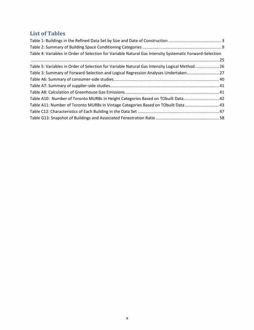
List of Tables Table 1: Buildings in the Refined Data Set by Size and Date of Construction .............................................. 3
Table 2: Summary of Building Space Conditioning Categories ..................................................................... 9
Table 4: Variables in Order of Selection for Variable Natural Gas Intensity Systematic Forward-Selection
.................................................................................................................................................................... 25
Table 5: Variables in Order of Selection for Variable Natural Gas Intensity Logical Method ..................... 26
Table 3: Summary of Forward-Selection and Logical Regression Analyses Undertaken ............................ 27
Table A6: Summary of consumer-side studies ............................................................................................ 40
Table A7: Summary of supplier-side studies ............................................................................................... 41
Table A8: Calculation of Greenhouse Gas Emissions .................................................................................. 41
Table A10: Number of Toronto MURBs in Height Categories Based on TObuilt Data ............................... 42
Table A11: Number of Toronto MURBs in Vintage Categories Based on TObuilt Data .............................. 43
Table C12: Characteristics of Each Building in the Data Set ....................................................................... 47
Table G13: Snapshot of Buildings and Associated Fenestration Ratio ....................................................... 58

1
1 Background Multi-unit residential buildings (MURBs) represent the most significant component in the Toronto
residential building inventory. Over half (56%) of the dwellings in the City of Toronto consist of MURBs.
As shown in Figure 1, a large proportion of all Toronto dwellings, 39%, are either mid-rise or high-rise
MURBs of five or more storeys. Low-rise MURBs of four storeys or fewer represent 17% of the dwellings
in the City of Toronto (Appendix A: Section 1).
Figure 1: Number of Dwellings by Type in Toronto
Figure Source: (City of Toronto, 2012)
Since MURBs are the most common form of dwelling in Toronto, it is not surprising that they are also a
significant source of greenhouse gas (GHG) emissions. On an annual basis, combined electricity and
natural gas consumption of Toronto MURBs result in an estimated 2.5M tonnes of eCO2 emissions
(Appendix A: Section 3). Mid- and high-rise MURBs are responsible for 68% of these emissions and low-
rise MURBs are responsible for 32% (Appendix A: Section 2). This is in line with another published
estimate that Toronto MURBs erected between 1945 and 1984 are responsible for between 2.0M and
2.2M tonnes of eCO2 (Stewart, 2010).
Despite the significant contribution of MURBs to GHG emissions, there are conflicting data on the
energy intensity of this building stock, particularly between two groups of studies: supplier-sides studies
using data from utility providers and studies using data directly from energy consumers. The energy
intensity of MURBs in consumer-side studies was found to be consistently higher than the MURB energy
intensities derived from the supplier-side studies. Given the large number of MURBs, determining an
accurate estimate of energy intensity and developing an understanding of how to reduce energy use is
an important step in reducing GHG emissions associated with this sector.
162,984 , 17%
379,700 , 39%
436,756 , 44%
Number of Dwellings by Type in Toronto
MURBs less than 5 storeys
MURBs 5 storeys or more
Other dwelling types

2
The first step toward the goal of reducing energy use is to generate reliable and consistent benchmarks
that characterize current energy use profiles. In determining consistency, new data must be compared
against existing data based on a similar method of data collection. For example, the data collected for
this study could be classified as a consumer-side study rather than a supplier-study. Thus, the data in
this study were only compared with consumer-side energy intensity figures. In establishing benchmarks,
a standardized process that categorizes buildings into groups with similar potential for improvement in
energy-efficiency is needed. This potential for energy-efficiency can then be used to prioritize the energy
retrofits for certain typologies and inform the development of policies and programs to address GHG
emissions in this sector.
1.1 Context and Structure of the Report This document is an interim report in the TAF-funded grant project called “The Energy Study of Toronto
Multi-Unit Residential Buildings” (the Energy Study). Conclusions and findings from this report will be
used to determine which building upgrades will be examined in the detailed typology-specific energy
study of the final phase of this project.
This study builds upon a previous study conducted by the authors, which was funded by the Toronto
Atmospheric Fund (TAF) and is entitled “Meta-Analysis of Energy Consumption in Multi-Unit Residential
Buildings in the Greater Toronto Area” (the Meta-Analysis). In the Meta-Analysis, energy consumption
information for 108 buildings in and around the Greater Toronto Area was analysed and correlations of
energy-use with building size, age and ownership type were sought. The Meta-Analysis was limited, in
part, because of the extent and completeness of the data.
The aim of this study is to address the data limitations of the Meta-Analysis by examining a refined data
set composed of buildings with more complete energy consumption and building characteristics data.
The following section describes the characteristics of the refined data set and identifies the sources of
data. Next, the methods used to weather normalize and analyze the data are presented. A discussion of
the established correlations is then provided followed by the results from a multi-variable regression
analysis. Anomalies revealed during the analysis are explored with an aim to better understand the
correlations and multi-variable regression results. The report then identifies four building categories
that will be the subject of a more detailed energy study in the next phase of this project. Finally the
conclusions are summarized and recommendations are put forth.
1.2 Data Collection and Data Sources The refined data set consists of 40 buildings and is composed of both newly acquired data as well as
select data from the Meta-Analysis. The methods used to choose these 40 buildings are outlined below.
Twenty new buildings were added to the data set. Two of the newly added MURBs were the focus of a
study by Tzekova et al. (2011) and three were the subject of a community energy plan for the City of
Toronto (Arup, 2010). Information on the remaining 15 newly added MURBs was obtained from energy
audit reports conducted by engineering consulting firms for projects being carried out by the Toronto
Atmospheric Fund.
3
Twenty buildings from the original Meta-Analysis data set were also used in this report. The Meta-
Analysis data source that showed the greatest potential for inclusion in this investigation was TAF’s
Green Condo Champions Project. This data included four years of monthly natural gas consumption
information as well as energy audit reports for 40 buildings. However, electricity consumption
information was not contained within the original data set. To obtain this electricity data, contacts at
each of the 40 buildings were sent a letter asking for permission to acquire electricity consumption
information directly from Toronto Hydro. A sample of the letter seeking permission to access the data
as well as a Frequently Asked Questions (FAQs) sheet provided later in the process can be found inThe
number of MURBs in Toronto has been estimated based on the number of dwellings in the City of
Toronto as given in Appendix A: Section 1. The number of dwellings per building has been taken as the
median number of suites in the MURBs included in this study and the Meta-Analysis. The median
number of suites in MURBs less than four storeys was 36 and the median number of suites in MURBs
five storeys or greater was 181.
Estimated number of MURBs less than five storeys:
Estimated number of MURBs five storeys or greater:
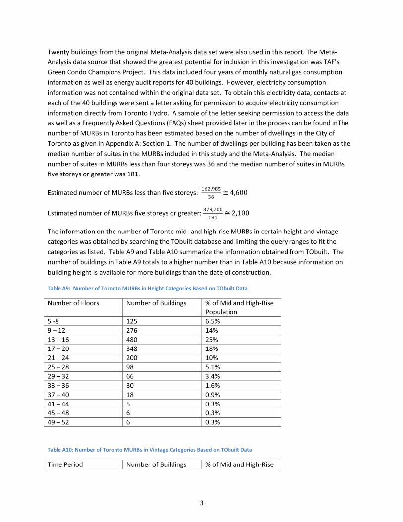
The information on the number of Toronto mid- and high-rise MURBs in certain height and vintage
categories was obtained by searching the TObuilt database and limiting the query ranges to fit the
categories as listed. Table A9 and Table A10 summarize the information obtained from TObuilt. The
number of buildings in Table A9 totals to a higher number than in Table A10 because information on
building height is available for more buildings than the date of construction.
Table A9: Number of Toronto MURBs in Height Categories Based on TObuilt Data
Number of Floors Number of Buildings % of Mid and High-Rise Population
5 -8 125 6.5%
9 – 12 276 14%
13 – 16 480 25%
17 – 20 348 18%
21 – 24 200 10%
25 – 28 98 5.1%
29 – 32 66 3.4%
33 – 36 30 1.6%
37 – 40 18 0.9%
41 – 44 5 0.3%
45 – 48 6 0.3%
49 – 52 6 0.3%
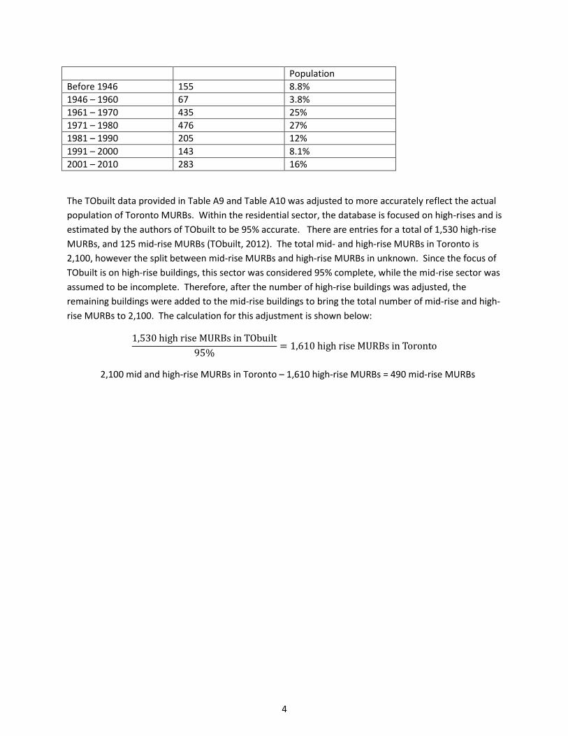
Table A10: Number of Toronto MURBs in Vintage Categories Based on TObuilt Data
Time Period Number of Buildings % of Mid and High-Rise
4
Population
Before 1946 155 8.8%
1946 – 1960 67 3.8%
1961 – 1970 435 25%
1971 – 1980 476 27%
1981 – 1990 205 12%
1991 – 2000 143 8.1%
2001 – 2010 283 16%
The TObuilt data provided in Table A9 and Table A10 was adjusted to more accurately reflect the actual
population of Toronto MURBs. Within the residential sector, the database is focused on high-rises and is
estimated by the authors of TObuilt to be 95% accurate. There are entries for a total of 1,530 high-rise
MURBs, and 125 mid-rise MURBs (TObuilt, 2012). The total mid- and high-rise MURBs in Toronto is
2,100, however the split between mid-rise MURBs and high-rise MURBs in unknown. Since the focus of
TObuilt is on high-rise buildings, this sector was considered 95% complete, while the mid-rise sector was
assumed to be incomplete. Therefore, after the number of high-rise buildings was adjusted, the
remaining buildings were added to the mid-rise buildings to bring the total number of mid-rise and high-
rise MURBs to 2,100. The calculation for this adjustment is shown below:
2,100 mid and high-rise MURBs in Toronto – 1,610 high-rise MURBs = 490 mid-rise MURBs
5
Appendix B. Permission to access electricity consumption information for nine of the 40 buildings was
eventually obtained. In four of these nine buildings, residents were metered individually and only
permission for access to common electricity consumption could be obtained. Therefore, only five
buildings in the refined data set come from the Green Condo Champions Project.
To obtain more buildings for this study, some of the High Rise Building Statistically Representative
(HiSTAR) buildings (Liu, 2007) used in the original Meta-Analysis were selected. Although the HiSTAR
data contained electricity and natural gas consumption information for 55 Ontario buildings, quality and
completeness of the data were found to be variable. As well, not all of the buildings were located in the
City of Toronto. Only HiSTAR buildings that met the following criteria were included in this study:
The building had to be located in the City of Toronto;
More than eight months of natural gas and electricity consumption data had to be available;
When weather normalization was carried out, a coefficient of determination (R2) greater than
0.8 had to be achieved for the energy source providing the primary heating (usually natural gas).
Upon examining the HiSTAR data, 15 of the 55 buildings used in the Meta-Analysis were considered
adequate for inclusion in this study.
2 Description of Data Characteristics This section summarizes characteristics of the data with respect to general building characteristics and
introduces some limitations which must be considered when reviewing the results of this study.
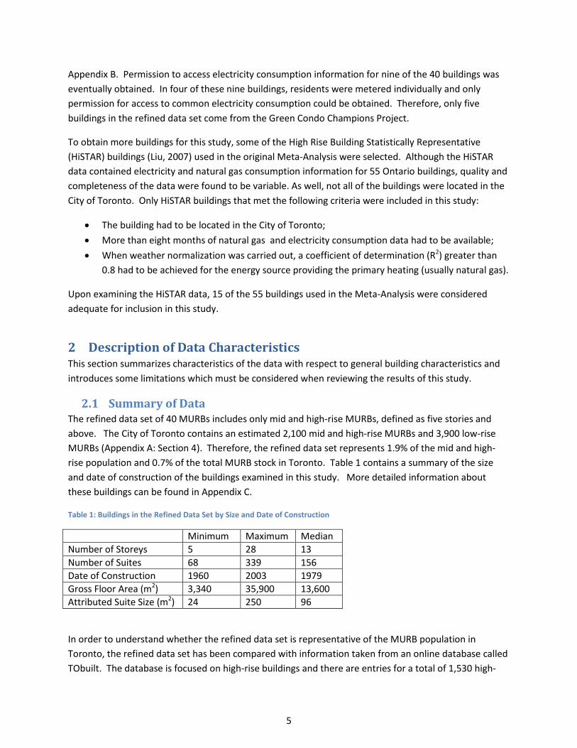
2.1 Summary of Data The refined data set of 40 MURBs includes only mid and high-rise MURBs, defined as five stories and
above. The City of Toronto contains an estimated 2,100 mid and high-rise MURBs and 3,900 low-rise
MURBs (Appendix A: Section 4). Therefore, the refined data set represents 1.9% of the mid and high-
rise population and 0.7% of the total MURB stock in Toronto. Table 1 contains a summary of the size
and date of construction of the buildings examined in this study. More detailed information about
these buildings can be found in Appendix C.
Table 1: Buildings in the Refined Data Set by Size and Date of Construction
Minimum Maximum Median
Number of Storeys 5 28 13
Number of Suites 68 339 156
Date of Construction 1960 2003 1979
Gross Floor Area (m2) 3,340 35,900 13,600
Attributed Suite Size (m2) 24 250 96
In order to understand whether the refined data set is representative of the MURB population in
Toronto, the refined data set has been compared with information taken from an online database called
TObuilt. The database is focused on high-rise buildings and there are entries for a total of 1,530 high-
6
rise MURBs, and 125 mid-rise MURBs (TObuilt, 2012). The raw data taken from TObuilt is provided in
Appendix A: Section 4. As well, an explanation as to how the TObuilt data has been weighted to account
for its limited data on mid-rise buildings and represent the actual number of MURBs (the population) in
the City of Toronto is provided in Appendix A.
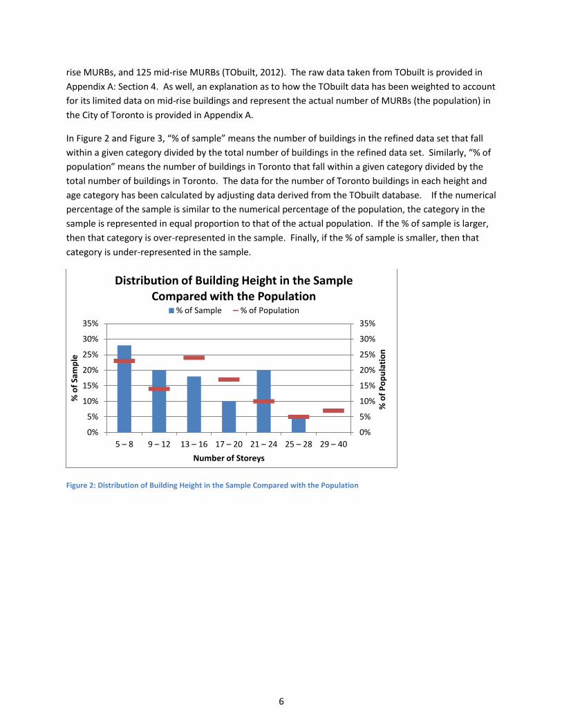
In Figure 2 and Figure 3, “% of sample” means the number of buildings in the refined data set that fall
within a given category divided by the total number of buildings in the refined data set. Similarly, “% of
population” means the number of buildings in Toronto that fall within a given category divided by the
total number of buildings in Toronto. The data for the number of Toronto buildings in each height and
age category has been calculated by adjusting data derived from the TObuilt database. If the numerical
percentage of the sample is similar to the numerical percentage of the population, the category in the
sample is represented in equal proportion to that of the actual population. If the % of sample is larger,
then that category is over-represented in the sample. Finally, if the % of sample is smaller, then that
category is under-represented in the sample.
Figure 2: Distribution of Building Height in the Sample Compared with the Population
0%
5%
10%
15%
20%
25%
30%
35%
0%
5%
10%
15%
20%
25%
30%
35%
5 – 8 9 – 12 13 – 16 17 – 20 21 – 24 25 – 28 29 – 40
% o
f P
op
ula
tio
n
% o
f Sa
mp
le
Number of Storeys
Distribution of Building Height in the Sample Compared with the Population
% of Sample % of Population
7
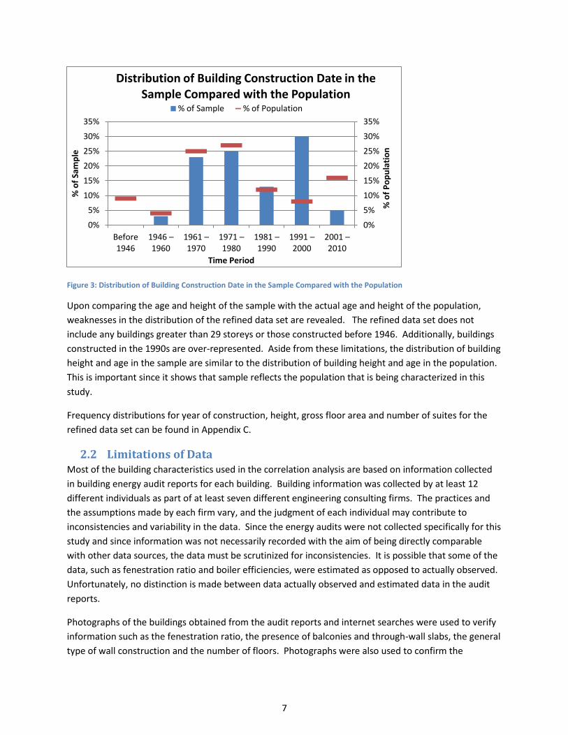
Figure 3: Distribution of Building Construction Date in the Sample Compared with the Population
Upon comparing the age and height of the sample with the actual age and height of the population,
weaknesses in the distribution of the refined data set are revealed. The refined data set does not
include any buildings greater than 29 storeys or those constructed before 1946. Additionally, buildings
constructed in the 1990s are over-represented. Aside from these limitations, the distribution of building
height and age in the sample are similar to the distribution of building height and age in the population.
This is important since it shows that sample reflects the population that is being characterized in this
study.
Frequency distributions for year of construction, height, gross floor area and number of suites for the
refined data set can be found in Appendix C.
2.2 Limitations of Data Most of the building characteristics used in the correlation analysis are based on information collected
in building energy audit reports for each building. Building information was collected by at least 12
different individuals as part of at least seven different engineering consulting firms. The practices and
the assumptions made by each firm vary, and the judgment of each individual may contribute to
inconsistencies and variability in the data. Since the energy audits were not collected specifically for this
study and since information was not necessarily recorded with the aim of being directly comparable
with other data sources, the data must be scrutinized for inconsistencies. It is possible that some of the
data, such as fenestration ratio and boiler efficiencies, were estimated as opposed to actually observed.
Unfortunately, no distinction is made between data actually observed and estimated data in the audit
reports.
Photographs of the buildings obtained from the audit reports and internet searches were used to verify
information such as the fenestration ratio, the presence of balconies and through-wall slabs, the general
type of wall construction and the number of floors. Photographs were also used to confirm the
0%
5%
10%
15%
20%
25%
30%
35%
0%
5%
10%
15%
20%
25%
30%
35%
Before 1946
1946 – 1960
1961 – 1970
1971 – 1980
1981 – 1990
1991 – 2000
2001 – 2010
% o
f P
op
ula
tio
n
% o
f Sa
mp
le
Time Period
Distribution of Building Construction Date in the Sample Compared with the Population
% of Sample % of Population
8
presence of window unit air conditioners and roof equipment such as make-up air units. Searches on
the building address were used to obtain more information about the ownership type (seniors’ home,
hospice, co-operative housing organization) and the presence of amenities such as a pool or fitness
facility. Finally, census information combined with the number of suites was used to estimate the
number of occupants. The effect of the limitations of the data will be discussed further as each variable
is examined in the correlations analysis.
3 Methodology This section outlines how the data were processed to allow for comparison between buildings. It also
discusses how the methodology in this report differs from the Meta-Analysis and how extreme outliers
have been considered and resolved. For each of the 40 buildings, monthly natural gas and electricity
data were weather normalized using a standard weather year as determined from the Canadian
Weather for Energy Calculations (CWEC). At this point, outliers were identified for further investigation
in Section 5. Following the weather normalization, the base (weather independent) component and the
variable (weather dependent) component of the natural gas and electricity consumption were
identified. To ensure buildings with the same heating systems were compared against one another,
buildings were allocated to one of three groups: natural gas heating, electric heating or a combination
system. Then, using the normalized energy data organized in these groups, functional relationships
between the variables relating to the mechanical and the electrical system, the building envelope, and
the occupancy characteristics of the building were sought. These individual variables were tested
against various measures of energy use to determine where correlations existed. Then a multi-variable
regression analysis was conducted to determine the influence of a combination of variables. Finally,
buildings that appeared to be anomalies from the identified trends were examined in greater detail.
3.1 Weather Normalization Since heating and cooling demands vary from year to year, the energy consumption data had to be
‘weather normalized’ in order to compare the natural gas and electricity data from different years. By
weather normalizing this consumption data, fluctuations in energy consumption due to weather
variations can be eliminated.
The weather dependency of natural gas use is only related to heating and was therefore weather
normalized using heating degree days (HDDs) only. However, electricity consumption can be related to
air conditioning loads as well as heating loads depending on the heating energy type. As such, electricity
use data were weather normalized considering both HDDs and cooling degree days (CDDs). Therefore,
three weather normalization processes were completed on the electricity data. One normalization
process used HDDs only, one normalization process used CDDs only, and one normalization process
used HDDs for the winter months (October to March) and CDDs for the summer months (April to
September). The normalization process that yielded the highest coefficient of determination (R2 value)
was the normalization process that was selected for use in this study. A full description of the weather
normalization process and assumptions is provided in Appendix D.
9
The CWEC standard weather year is based on the average weather data in Toronto for a 30-year time
period from 1960-1989. The standard weather year is substantially colder than the weather from 1998
to 2011, which are generally the years for which the energy consumption data in this data set apply.
Since the standard weather year is colder, the heating load for each building increases after the data are
weather normalized. Therefore, energy consumption data from this study may appear higher than
energy consumption in other studies and cannot be directly compared since the data may not have been
weather normalized or it may have been weather normalized using a different base year.
3.2 Rejection of Outliers The natural gas and electricity consumption data were obtained from the billed energy use for each of
the buildings in the data set. Prior to weather normalization, outliers in the energy use data were
removed. Outliers can sometimes occur when the billed energy use does not reflect the actual energy
use in the period. A common circumstance in which billed data does not align with actual energy use is
when meter readings are estimated by the utility companies. In such cases, outliers can arise,
particularly where the actual meter reading and the billing correction is not made for a few months.
Outliers can also occur when building systems are shut down for replacement or maintenance. In some
cases, occupant behaviour can be responsible for outliers in the energy consumption data. Finally,
errors in data entry can also be a source of outliers.
Outliers were removed when energy consumption was plotted against HDDs or CDDs in the weather
normalization process. Removal was based on the following criteria:
When an electricity consumption datum was more than 20% different from the predicted
electricity consumption as determined by the equation for the line of best fit, it was removed.
When a natural gas consumption datum was more than 30% different from the predicted
natural gas consumption as determined the equation for the line of best fit, it was removed.
A few of the buildings had energy consumption data that appeared to contain outliers for the same two
to four months of the year for every year of data. To avoid removing too many outliers and leaving a
gap in the data, each calendar month where the data showed the lowest error was preserved and
included in the weather normalization. Therefore, a rule was developed that a monthly datum was only
removed as long as all 12 calendar months were still represented after its removal.
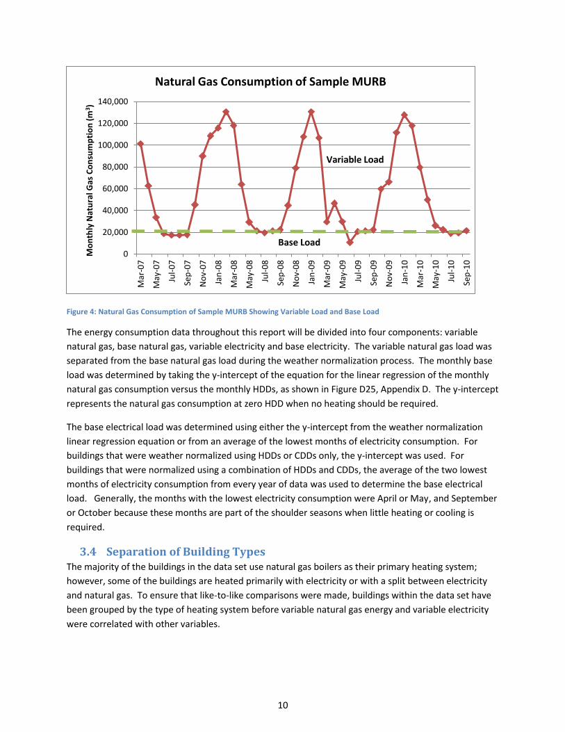
3.3 Determination of Energy Load Types When energy consumption is examined on a monthly basis, it can be separated into two components as
illustrated in Figure 4: the base loads (weather independent) and the variable loads (weather
dependent). Although lighting use, domestic hot water use and plug-loads can show minor seasonal
fluctuations and although these energy uses contribute to heating the building, these seasonal
fluctuations are considered negligible compared with the seasonal variations resulting from operating
the heating and cooling systems.
10
Figure 4: Natural Gas Consumption of Sample MURB Showing Variable Load and Base Load
The energy consumption data throughout this report will be divided into four components: variable
natural gas, base natural gas, variable electricity and base electricity. The variable natural gas load was
separated from the base natural gas load during the weather normalization process. The monthly base
load was determined by taking the y-intercept of the equation for the linear regression of the monthly
natural gas consumption versus the monthly HDDs, as shown in Figure D25, Appendix D. The y-intercept
represents the natural gas consumption at zero HDD when no heating should be required.
The base electrical load was determined using either the y-intercept from the weather normalization
linear regression equation or from an average of the lowest months of electricity consumption. For
buildings that were weather normalized using HDDs or CDDs only, the y-intercept was used. For
buildings that were normalized using a combination of HDDs and CDDs, the average of the two lowest
months of electricity consumption from every year of data was used to determine the base electrical
load. Generally, the months with the lowest electricity consumption were April or May, and September
or October because these months are part of the shoulder seasons when little heating or cooling is
required.
3.4 Separation of Building Types The majority of the buildings in the data set use natural gas boilers as their primary heating system;
however, some of the buildings are heated primarily with electricity or with a split between electricity
and natural gas. To ensure that like-to-like comparisons were made, buildings within the data set have
been grouped by the type of heating system before variable natural gas energy and variable electricity
were correlated with other variables.
0
20,000
40,000
60,000
80,000
100,000
120,000
140,000
Mar
-07
May
-07
Jul-
07
Sep
-07
No
v-0
7
Jan
-08
Mar
-08
May
-08
Jul-
08
Sep
-08
No
v-0
8
Jan
-09
Mar
-09
May
-09
Jul-
09
Sep
-09
No
v-0
9
Jan
-10
Mar
-10
May
-10
Jul-
10
Sep
-10
Mo
nth
ly N
atu
ral G
as C
on
sum
pti
on
(m
3)
Natural Gas Consumption of Sample MURB
Base Load
Variable Load
11
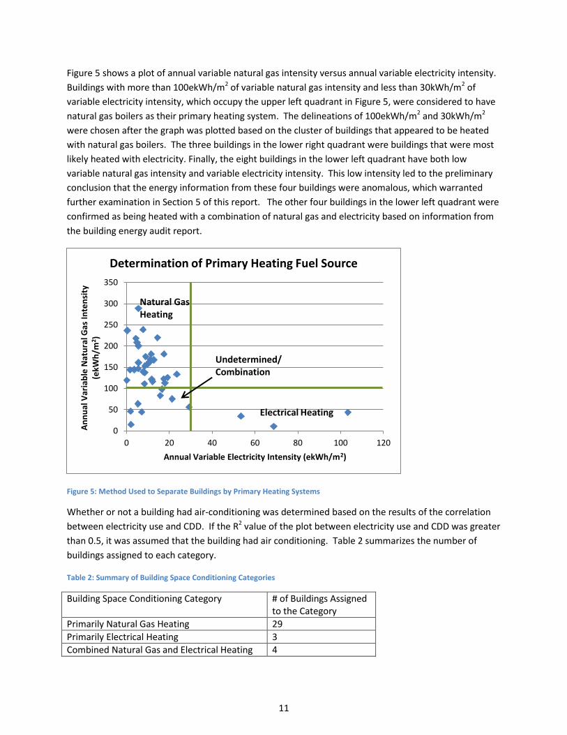
Figure 5 shows a plot of annual variable natural gas intensity versus annual variable electricity intensity.
Buildings with more than 100ekWh/m2 of variable natural gas intensity and less than 30kWh/m2 of
variable electricity intensity, which occupy the upper left quadrant in Figure 5, were considered to have
natural gas boilers as their primary heating system. The delineations of 100ekWh/m2 and 30kWh/m2
were chosen after the graph was plotted based on the cluster of buildings that appeared to be heated
with natural gas boilers. The three buildings in the lower right quadrant were buildings that were most
likely heated with electricity. Finally, the eight buildings in the lower left quadrant have both low
variable natural gas intensity and variable electricity intensity. This low intensity led to the preliminary
conclusion that the energy information from these four buildings were anomalous, which warranted
further examination in Section 5 of this report. The other four buildings in the lower left quadrant were
confirmed as being heated with a combination of natural gas and electricity based on information from
the building energy audit report.
Figure 5: Method Used to Separate Buildings by Primary Heating Systems
Whether or not a building had air-conditioning was determined based on the results of the correlation
between electricity use and CDD. If the R2 value of the plot between electricity use and CDD was greater
than 0.5, it was assumed that the building had air conditioning. Table 2 summarizes the number of
buildings assigned to each category.
Table 2: Summary of Building Space Conditioning Categories
Building Space Conditioning Category # of Buildings Assigned to the Category
Primarily Natural Gas Heating 29
Primarily Electrical Heating 3
Combined Natural Gas and Electrical Heating 4
0
50
100
150
200
250
300
350
0 20 40 60 80 100 120
An
nu
al V
aria
ble
Nat
ura
l Gas
In
ten
sity
(e
kWh
/m2 )
Annual Variable Electricity Intensity (ekWh/m2)
Determination of Primary Heating Fuel Source
Natural Gas Heating
Electrical Heating
Undetermined/ Combination
12
Air Conditioned Buildings 11
Buildings with Undetermined Heating Systems 4
3.5 Regression Analysis With the data weather normalized and organized into groups of buildings with similar heating system
types, variables related to building characteristics were plotted against base and variable natural gas
consumption and total electricity consumption. A discussion of the particular variables correlated with
each load type can be found in Section 4.2. The coefficient of determination, or R2 value, was used as a
means of evaluating how well the linear regression line explains the variation in the energy consumption
data.
3.6 Multi-variable Regression Analysis The multi-variable regression analysis was completed in Microsoft Excel using the regression function
from the Analysis ToolPak Add-In. A stepwise forward-selection approach to maximize the adjusted R2
value was used for each regression analysis.
The adjusted R2 value derived from the multi-variable regression analyses is the same as the R2 value in
the single variable regression analysis except that a correction has been made to account for the
number of variables involved. As variables are added, more of the variation in the data should
automatically be explained; therefore, to account for the advantage of having additional variables, a
reduction factor is applied to the R2 value. This means that the adjusted R2 value is equal to the R2 value
in a single-variable regression, but is less than the R2 value when more than one variable is involved.
Each stepwise forward-selection approach to multi-variable regression analysis results in a linear
equation relating the selected variables to coefficients as follows:
y=c1xmax1+c2xmax2+c3xmax3+… cnxmaxn
where:
y = The component of energy use or energy intensity being examined
c = The coefficient resulting from the multi-variable regression analysis
x = The variable selected to maximize the R2 value
The multi-variable regression analysis involves the following steps:
1. All of the variables to be considered in the analysis are chosen. These variables are called x1,x2,
x3,…,xn and each analysis includes n variables. The variable “y” is the component of energy
consumption for which the regression is being completed.
2. A single-variable linear regression of y versus xi is completed for all n variables. The variable that
yields the highest adjusted R2 value for in the single-variable linear regression is designated
xmax1.

13
3. A double-variable linear regression of y versus xmax1 and all remaining xi is completed for all n-1
variables. The variable that yields the highest adjusted R2 value in the double variable linear
regression is designated xmax2. If the new maximum adjusted R2 value is smaller than the
maximum R2 value in the previous step, then the regression is complete and xmax1 is the only
variable involved in the final regression results. If the new maximum adjusted R2 value is larger
than the maximum R2 value in the previous step, then a triple variable regression must be
completed.
4. Variables continue to be added one at a time until the R2 value is maximized.
5. The final result is a linear equation relating the selected variables (xmax1, xmax2,…,etc.) to y using
coefficients.
An additional approach, based on the logic of which variables should govern each energy consumption
component, was also used to select the order in which variables were added for some of the regression
analyses.
4 Results and Discussion In the sections that follow, an overview of building energy intensity has been presented, followed by a
discussion of the variables that influence energy use. Then, energy consumption components (base and
variable natural gas and total electricity consumption) are correlated with these variables to show the
apparent influence. Finally, the results of the multi-variable regression analysis are presented.
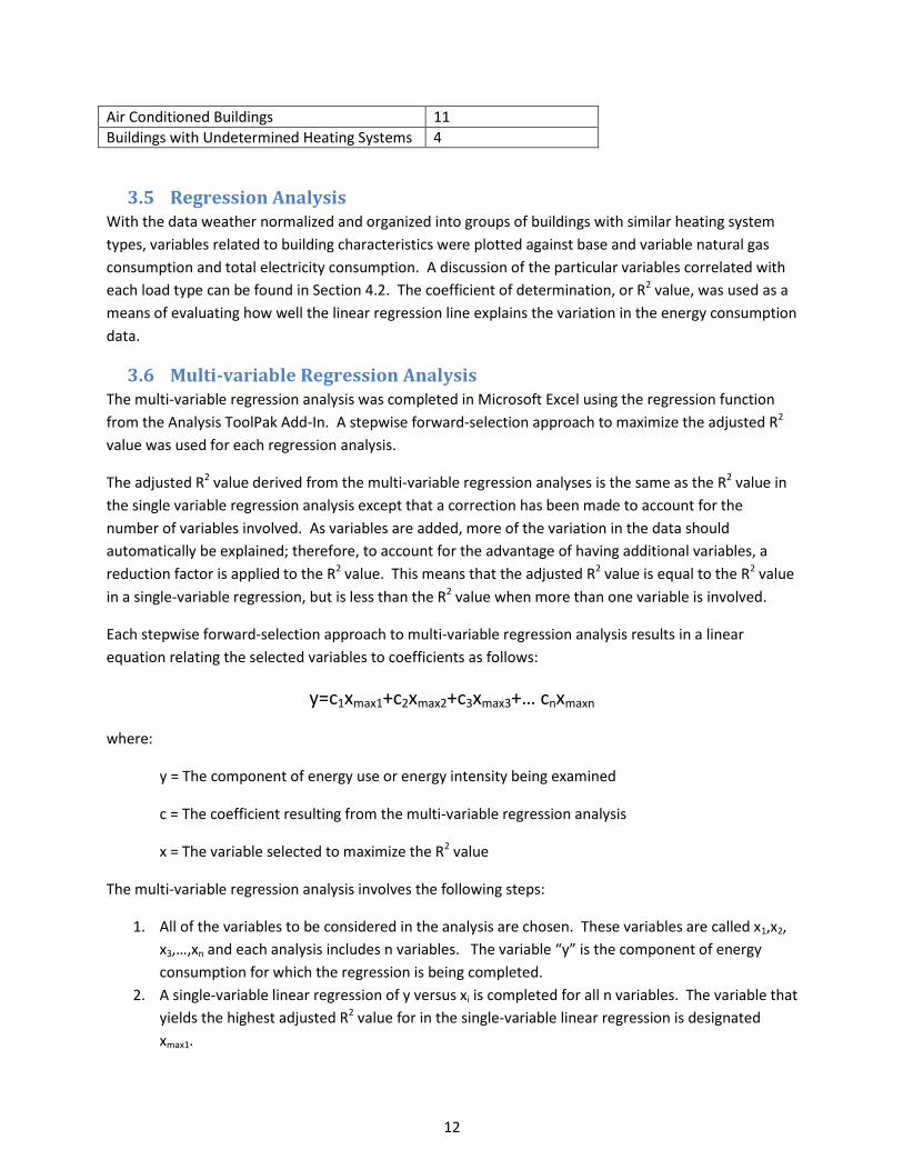
4.1 Energy Intensity Within the refined data set, which is focused on only mid- and high-rise MURBs, the total annual energy
consumption ranges from 1,125 eMWh to 12,190 eMWh. In order to facilitate comparisons between
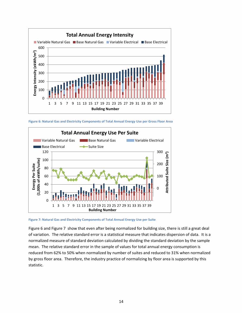
buildings, it is helpful to normalize the data based on building size. Figure 6 and Figure 7 show the
annual energy consumption on a per gross floor area (energy intensity) and a per suite basis,
respectively. The gross floor area is considered to be the total conditioned floor area within a building.
Generally, this includes the common areas, the corridors, and the individual suites. It typically does not
include underground parking, even if the parking area is conditioned to some degree. Although the
definition was not specified in the original building reports, it has been assumed that the gross floor
areas provided in energy audit reports is the total conditioned floor area.
14
Figure 6: Natural Gas and Electricity Components of Total Annual Energy Use per Gross Floor Area
Figure 7: Natural Gas and Electricity Components of Total Annual Energy Use per Suite
Figure 6 and Figure 7 show that even after being normalized for building size, there is still a great deal
of variation. The relative standard error is a statistical measure that indicates dispersion of data. It is a
normalized measure of standard deviation calculated by dividing the standard deviation by the sample
mean. The relative standard error in the sample of values for total annual energy consumption is
reduced from 62% to 50% when normalized by number of suites and reduced to 31% when normalized
by gross floor area. Therefore, the industry practice of normalizing by floor area is supported by this
statistic.
0
100
200
300
400
500
600
1 3 5 7 9 11 13 15 17 19 21 23 25 27 29 31 33 35 37 39
Ene
rgy
Inte
nsi
ty (
ekW
h/m
2 )
Building Number
Total Annual Energy Intensity Variable Natural Gas Base Natural Gas Variable Electrical Base Electrical
-100
0
100
200
300
0
20
40
60
80
100
120
1 3 5 7 9 11 13 15 17 19 21 23 25 27 29 31 33 35 37 39
Att
rib
ute
d S
uit
e S
ize
(m
2 )
Ene
rgy
Pe
r Su
ite
(1
,00
0s
of
ekW
h/s
uit
e)
Building Number
Total Annual Energy Use Per Suite
Variable Natural Gas Base Natural Gas Variable Electrical
Base Electrical Suite Size
15
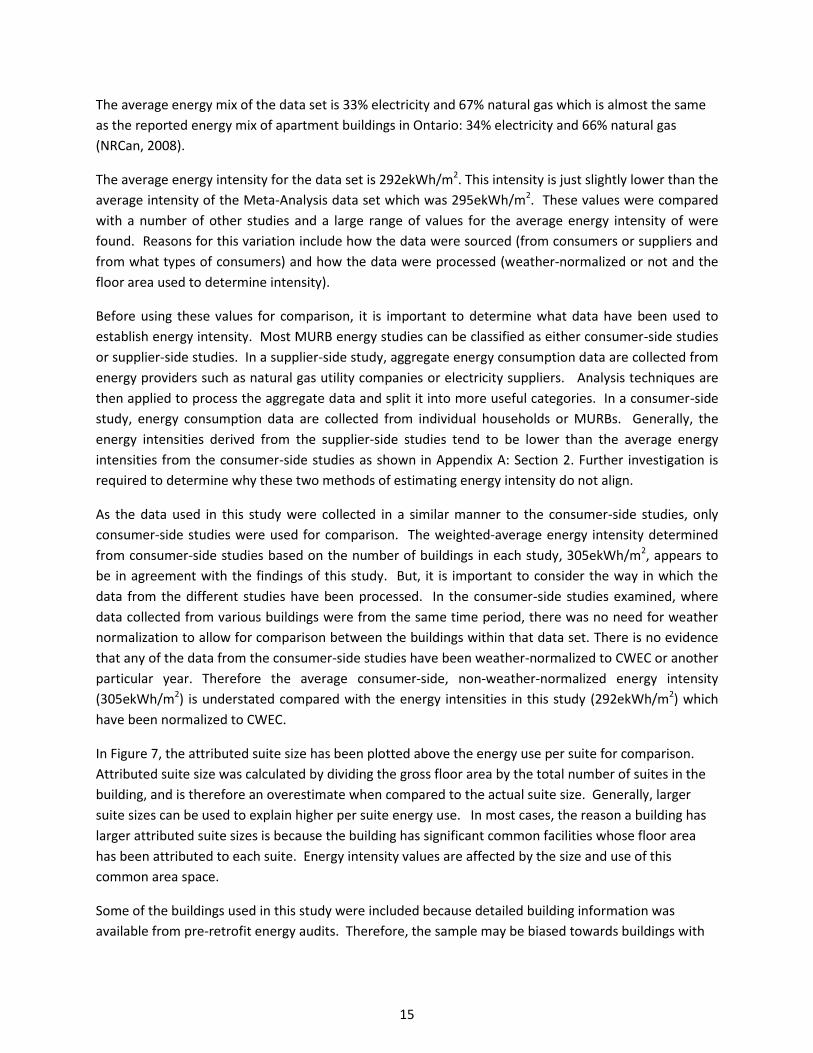
The average energy mix of the data set is 33% electricity and 67% natural gas which is almost the same
as the reported energy mix of apartment buildings in Ontario: 34% electricity and 66% natural gas
(NRCan, 2008).
The average energy intensity for the data set is 292ekWh/m2. This intensity is just slightly lower than the
average intensity of the Meta-Analysis data set which was 295ekWh/m2. These values were compared
with a number of other studies and a large range of values for the average energy intensity of were
found. Reasons for this variation include how the data were sourced (from consumers or suppliers and
from what types of consumers) and how the data were processed (weather-normalized or not and the
floor area used to determine intensity).
Before using these values for comparison, it is important to determine what data have been used to
establish energy intensity. Most MURB energy studies can be classified as either consumer-side studies
or supplier-side studies. In a supplier-side study, aggregate energy consumption data are collected from
energy providers such as natural gas utility companies or electricity suppliers. Analysis techniques are
then applied to process the aggregate data and split it into more useful categories. In a consumer-side
study, energy consumption data are collected from individual households or MURBs. Generally, the
energy intensities derived from the supplier-side studies tend to be lower than the average energy
intensities from the consumer-side studies as shown in Appendix A: Section 2. Further investigation is
required to determine why these two methods of estimating energy intensity do not align.
As the data used in this study were collected in a similar manner to the consumer-side studies, only
consumer-side studies were used for comparison. The weighted-average energy intensity determined
from consumer-side studies based on the number of buildings in each study, 305ekWh/m2, appears to
be in agreement with the findings of this study. But, it is important to consider the way in which the
data from the different studies have been processed. In the consumer-side studies examined, where
data collected from various buildings were from the same time period, there was no need for weather
normalization to allow for comparison between the buildings within that data set. There is no evidence
that any of the data from the consumer-side studies have been weather-normalized to CWEC or another
particular year. Therefore the average consumer-side, non-weather-normalized energy intensity
(305ekWh/m2) is understated compared with the energy intensities in this study (292ekWh/m2) which
have been normalized to CWEC.
In Figure 7, the attributed suite size has been plotted above the energy use per suite for comparison.
Attributed suite size was calculated by dividing the gross floor area by the total number of suites in the
building, and is therefore an overestimate when compared to the actual suite size. Generally, larger
suite sizes can be used to explain higher per suite energy use. In most cases, the reason a building has
larger attributed suite sizes is because the building has significant common facilities whose floor area
has been attributed to each suite. Energy intensity values are affected by the size and use of this
common area space.
Some of the buildings used in this study were included because detailed building information was
available from pre-retrofit energy audits. Therefore, the sample may be biased towards buildings with

16
lower energy efficiency since building energy audits are typically sought by building owners or managers
who might be concerned with energy efficiency.
To summarize, the average energy intensity resulting from this study must be considered in the context
of the weather normalization. Weather normalization is necessary to compare building data from
different years so it is not possible to directly compare these results to other non-weather normalized
studies. As well, the size and use of common areas and the attitude of the participant building owners
and managers to energy efficiency can also affect energy intensity calculations.
4.2 Selection of Variables As normalization by building size does not fully explain the variation in energy use, the purpose of this
section of the report is to determine what other variables have a correlation with the energy
consumption data. There are many variables that could contribute to the energy consumption within a
building. Variables related to occupant behaviour, mechanical and electrical systems, control systems,
building envelope, site environment, building management or demographics could all be involved. In
this study, the variables examined have been limited to physically measureable or observable variables
that were available in the building energy audit reports. Additionally, variables that would normally be
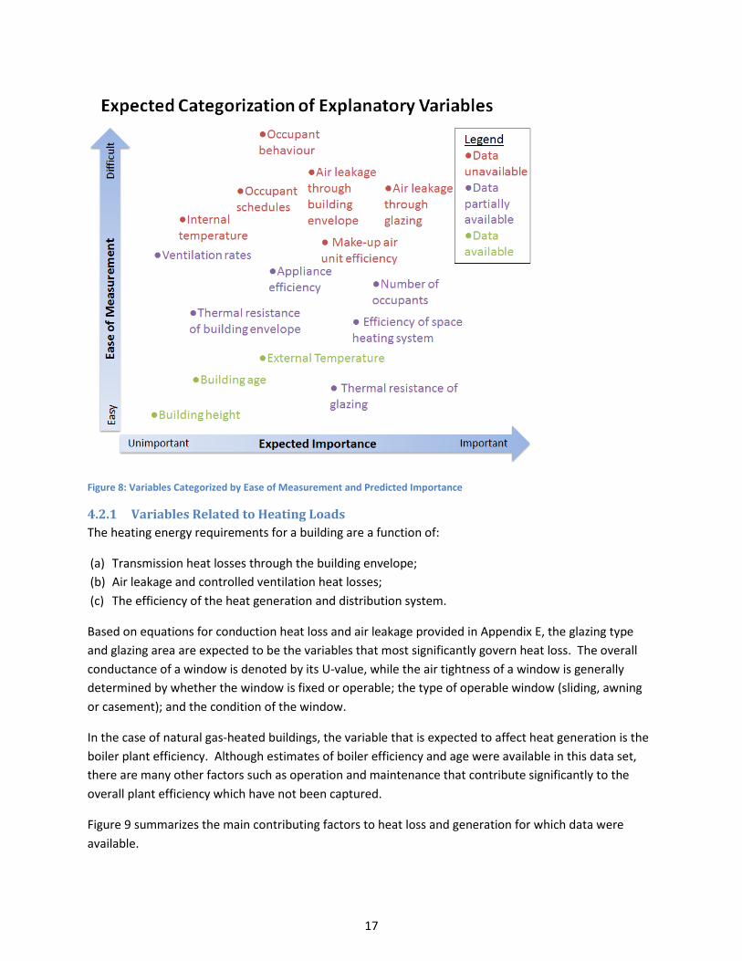
expected to have the greatest effect on the variation in energy consumption were investigated. Figure 8
provides a summary of possible variables and an indication of the data availability. Thermal glazing
characteristics, the efficiency of the space heating system and the number of occupants are the three
variables with the highest level of expected importance. In this figure, the expected importance of the
variables has been based on the initial belief that variables which affect heat loss and heat generation in
buildings should be well correlated with energy use.
17
Figure 8: Variables Categorized by Ease of Measurement and Predicted Importance
4.2.1 Variables Related to Heating Loads
The heating energy requirements for a building are a function of:
(a) Transmission heat losses through the building envelope;
(b) Air leakage and controlled ventilation heat losses;
(c) The efficiency of the heat generation and distribution system.
Based on equations for conduction heat loss and air leakage provided in Appendix E, the glazing type
and glazing area are expected to be the variables that most significantly govern heat loss. The overall
conductance of a window is denoted by its U-value, while the air tightness of a window is generally
determined by whether the window is fixed or operable; the type of operable window (sliding, awning
or casement); and the condition of the window.
In the case of natural gas-heated buildings, the variable that is expected to affect heat generation is the
boiler plant efficiency. Although estimates of boiler efficiency and age were available in this data set,
there are many other factors such as operation and maintenance that contribute significantly to the
overall plant efficiency which have not been captured.
Figure 9 summarizes the main contributing factors to heat loss and generation for which data were
available.

18
Figure 9: Variables Dominating Building Heating Requirements
4.2.2 Variables Related to Cooling Loads
Similar to heating, cooling loads are affected primarily by heat gain through the building envelope, heat
gain through both ventilation and air leakage, and the efficiency of the cooling system. In addition to
being influenced by conduction and air leakage through the glazing, solar heat gains due to radiation
through the glazing are also expected to have a significant effect. Based on the equation for radiation
heat transfer found in Appendix E, the two variables with the greatest effect are the glazing area and the
solar heat gain coefficient (SHGC) of the glass. With a higher SHGC, more radiation can penetrate the
building and heat it up so there is a higher cooling load.
4.2.3 Variables Related to Base Loads
Base loads are generally expected to be a function of the number of occupants, the gross floor area and
equipment efficiencies. Domestic hot water use and plug loads are most closely related to the number
of occupants because the activity of each occupant defines the magnitude of these loads. Lighting, fan,
and pump loads are most closely related to the gross floor area because the size of the interior space
defines the magnitude of loads. Since heating and cooling equipment efficiencies are often difficult to
obtain, building age may be used as a proxy so long as the building has not undergone any significant
renovations. Therefore, the following relationships were expected:
4.3 Regression Analysis Results This section presents a selection of correlations between the weather-normalized energy use data and a
number of building characteristics. Only significant findings have been presented in the body of this
report. For completeness, however, the results of the investigations which did not yield a reasonable
correlation have been presented in Appendix F.
4.3.1 Window Characteristics
The first variables examined in the correlation analysis were related to the window characteristics. As
explained in Section 4.2, window area, air tightness, thermal conductance, and SHGC of windows are
expected to influence both heating and cooling loads.
19
Some of the plots include buildings which have been identified as outliers. These anomalies will be
examined in Section 5 of the report. The line-of-best-fit plot applies only to data points that are not
considered outliers.
4.3.1.1 Fenestration-to-Wall Ratio
The fenestration-to-wall ratio (fenestration ratio) is the area of the exterior walls of the building covered
in glazing divided by the total wall surface area. Although the fenestration ratio for each building was
stated in many of the audit reports, it was often based on an estimate. Estimates of the fenestration
ratio were checked and modified as necessary by comparing the stated fenestration ratio with building
photographs. By comparing photographs of the various buildings, fenestration ratios were corrected so
that similar buildings had similar fenestration ratios.
Since much of the building information obtained for this study was provided on the condition that the
building identity remains confidential, full building photographs could not be provided in this report.
However, close-up photos which maintain the anonymity of the buildings have been provided in
Appendix G. In addition to the photographs, the originally estimated fenestration ratios as well as the
revised estimate of the fenestration ratios have been provided for each building. Figure 10, Figure 11,
and Figure 12 are all based on the revised estimate of fenestration ratios.
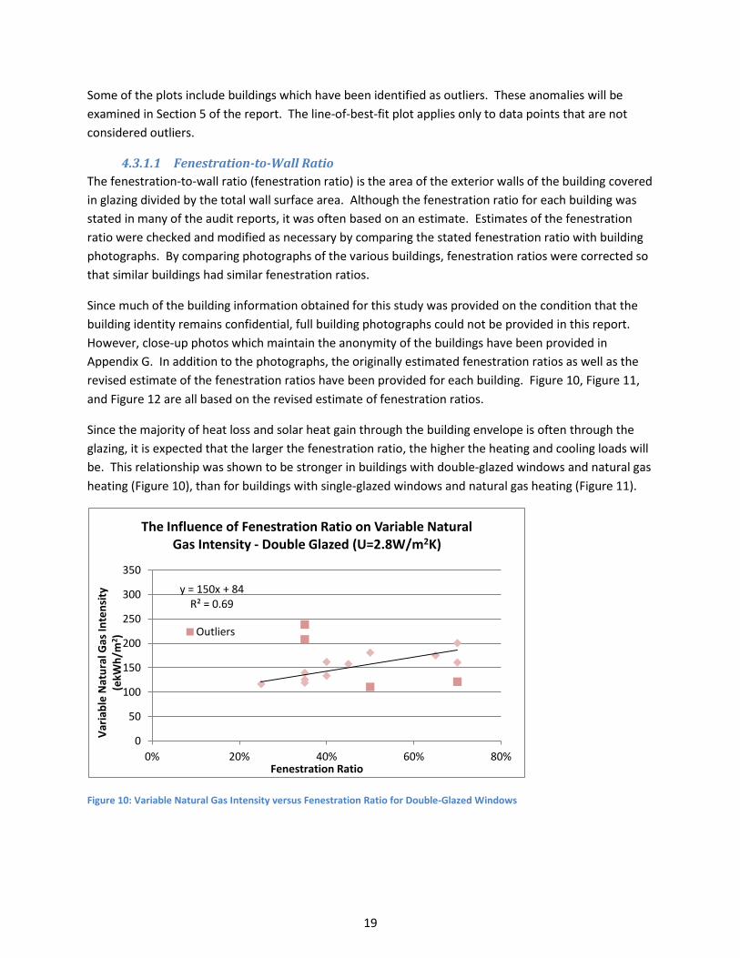
Since the majority of heat loss and solar heat gain through the building envelope is often through the
glazing, it is expected that the larger the fenestration ratio, the higher the heating and cooling loads will
be. This relationship was shown to be stronger in buildings with double-glazed windows and natural gas
heating (Figure 10), than for buildings with single-glazed windows and natural gas heating (Figure 11).
Figure 10: Variable Natural Gas Intensity versus Fenestration Ratio for Double-Glazed Windows
y = 150x + 84 R² = 0.69
0
50
100
150
200
250
300
350
0% 20% 40% 60% 80%
Var
iab
le N
atu
ral G
as In
ten
sity
(e
kWh
/m2 )
Fenestration Ratio
The Influence of Fenestration Ratio on Variable Natural Gas Intensity - Double Glazed (U=2.8W/m2K)
Outliers
20
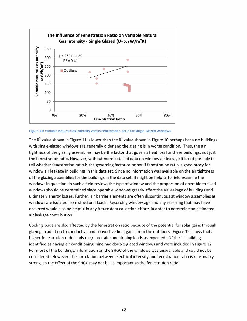
Figure 11: Variable Natural Gas Intensity versus Fenestration Ratio for Single-Glazed Windows
The R2 value shown in Figure 11 is lower than the R2 value shown in Figure 10 perhaps because buildings
with single-glazed windows are generally older and the glazing is in worse condition. Thus, the air
tightness of the glazing assemblies may be the factor that governs heat loss for these buildings, not just
the fenestration ratio. However, without more detailed data on window air leakage it is not possible to
tell whether fenestration ratio is the governing factor or rather if fenestration ratio is good proxy for
window air leakage in buildings in this data set. Since no information was available on the air tightness
of the glazing assemblies for the buildings in the data set, it might be helpful to field examine the
windows in question. In such a field review, the type of window and the proportion of operable to fixed
windows should be determined since operable windows greatly affect the air leakage of buildings and
ultimately energy losses. Further, air barrier elements are often discontinuous at window assemblies as
windows are isolated from structural loads. Recording window age and any resealing that may have
occurred would also be helpful in any future data collection efforts in order to determine an estimated
air leakage contribution.
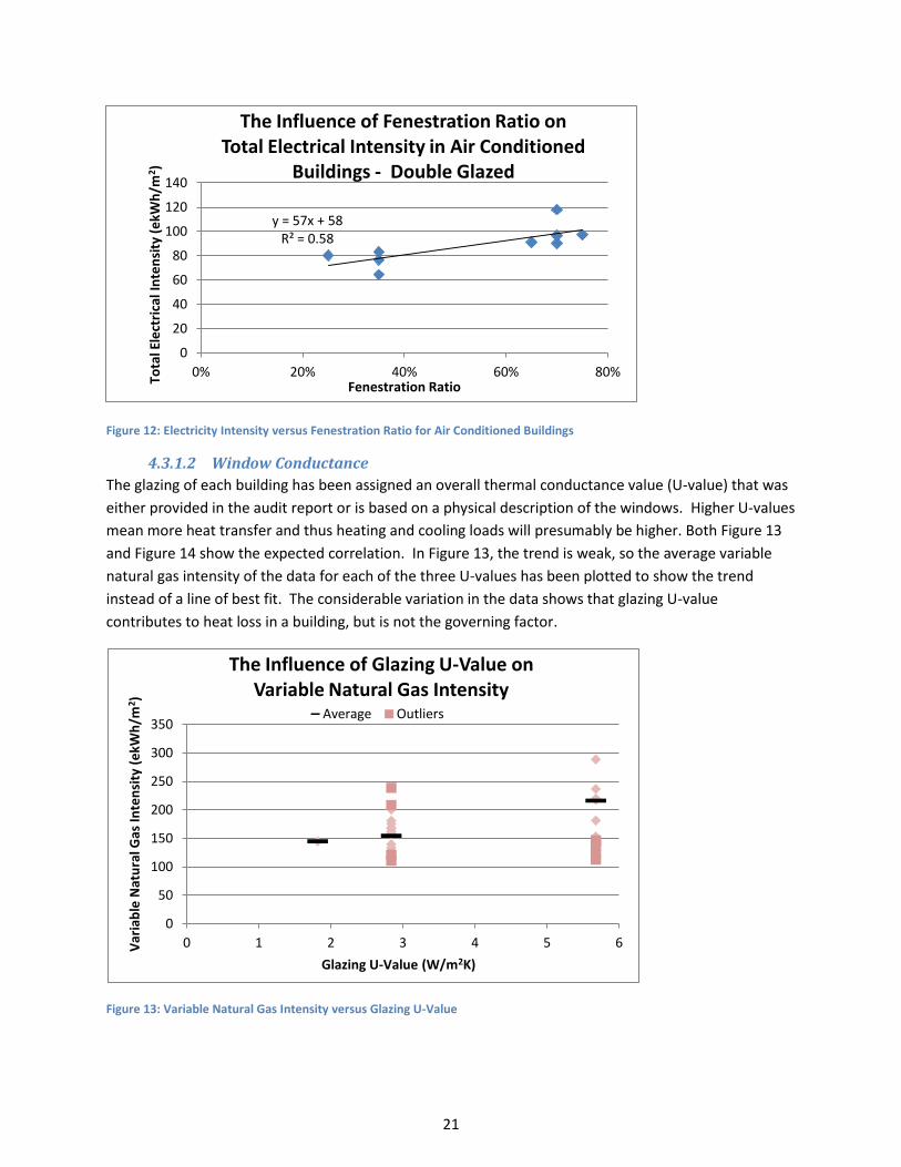
Cooling loads are also affected by the fenestration ratio because of the potential for solar gains through
glazing in addition to conductive and convective heat gains from the outdoors. Figure 12 shows that a
higher fenestration ratio leads to greater air conditioning loads as expected. Of the 11 buildings
identified as having air conditioning, nine had double-glazed windows and were included in Figure 12.
For most of the buildings, information on the SHGC of the windows was unavailable and could not be
considered. However, the correlation between electrical intensity and fenestration ratio is reasonably
strong, so the effect of the SHGC may not be as important as the fenestration ratio.
y = 250x + 120 R² = 0.41
0
50
100
150
200
250
300
350
0% 20% 40% 60% 80%
Var
iab
le N
atu
ral G
as In
ten
sity
(e
kWh
/m2 )
Fenestration Ratio
The Influence of Fenestration Ratio on Variable Natural Gas Intensity - Single Glazed (U=5.7W/m2K)
Outliers
21
Figure 12: Electricity Intensity versus Fenestration Ratio for Air Conditioned Buildings
4.3.1.2 Window Conductance
The glazing of each building has been assigned an overall thermal conductance value (U-value) that was
either provided in the audit report or is based on a physical description of the windows. Higher U-values
mean more heat transfer and thus heating and cooling loads will presumably be higher. Both Figure 13
and Figure 14 show the expected correlation. In Figure 13, the trend is weak, so the average variable
natural gas intensity of the data for each of the three U-values has been plotted to show the trend
instead of a line of best fit. The considerable variation in the data shows that glazing U-value
contributes to heat loss in a building, but is not the governing factor.
Figure 13: Variable Natural Gas Intensity versus Glazing U-Value
y = 57x + 58 R² = 0.58
0
20
40
60
80
100
120
140
0% 20% 40% 60% 80%
Tota
l Ele
ctri
cal I
nte
nsi
ty (
ekW
h/m
2 )
Fenestration Ratio
The Influence of Fenestration Ratio on Total Electrical Intensity in Air Conditioned
Buildings - Double Glazed
0
50
100
150
200
250
300
350
0 1 2 3 4 5 6 Var
iab
le N
atu
ral G
as In
ten
sity
(e
kWh
/m2)
Glazing U-Value (W/m2K)
The Influence of Glazing U-Value on Variable Natural Gas Intensity
Average Outliers
22
Figure 14: Electrical Intensity versus Glazing U-Value for Air Conditioned Buildings
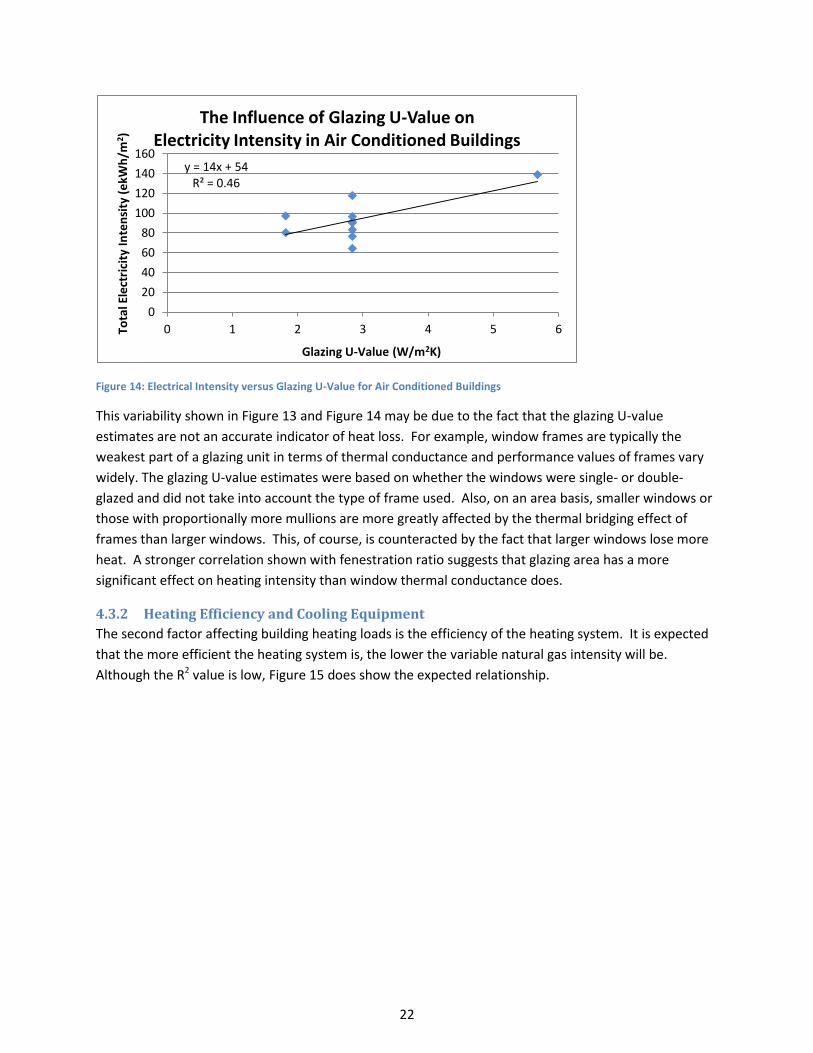
This variability shown in Figure 13 and Figure 14 may be due to the fact that the glazing U-value
estimates are not an accurate indicator of heat loss. For example, window frames are typically the
weakest part of a glazing unit in terms of thermal conductance and performance values of frames vary
widely. The glazing U-value estimates were based on whether the windows were single- or double-
glazed and did not take into account the type of frame used. Also, on an area basis, smaller windows or
those with proportionally more mullions are more greatly affected by the thermal bridging effect of
frames than larger windows. This, of course, is counteracted by the fact that larger windows lose more
heat. A stronger correlation shown with fenestration ratio suggests that glazing area has a more
significant effect on heating intensity than window thermal conductance does.
4.3.2 Heating Efficiency and Cooling Equipment
The second factor affecting building heating loads is the efficiency of the heating system. It is expected
that the more efficient the heating system is, the lower the variable natural gas intensity will be.
Although the R2 value is low, Figure 15 does show the expected relationship.
y = 14x + 54 R² = 0.46
0
20
40
60
80
100
120
140
160
0 1 2 3 4 5 6 Tota
l Ele
ctri
city
In
ten
sity
(e
kWh
/m2 )
Glazing U-Value (W/m2K)
The Influence of Glazing U-Value on Electricity Intensity in Air Conditioned Buildings
23
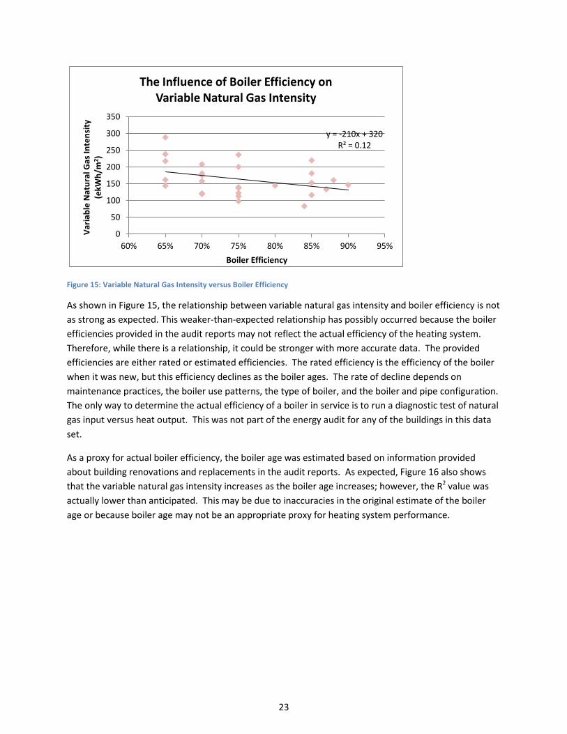
Figure 15: Variable Natural Gas Intensity versus Boiler Efficiency
As shown in Figure 15, the relationship between variable natural gas intensity and boiler efficiency is not
as strong as expected. This weaker-than-expected relationship has possibly occurred because the boiler
efficiencies provided in the audit reports may not reflect the actual efficiency of the heating system.
Therefore, while there is a relationship, it could be stronger with more accurate data. The provided
efficiencies are either rated or estimated efficiencies. The rated efficiency is the efficiency of the boiler
when it was new, but this efficiency declines as the boiler ages. The rate of decline depends on
maintenance practices, the boiler use patterns, the type of boiler, and the boiler and pipe configuration.
The only way to determine the actual efficiency of a boiler in service is to run a diagnostic test of natural
gas input versus heat output. This was not part of the energy audit for any of the buildings in this data
set.
As a proxy for actual boiler efficiency, the boiler age was estimated based on information provided
about building renovations and replacements in the audit reports. As expected, Figure 16 also shows
that the variable natural gas intensity increases as the boiler age increases; however, the R2 value was
actually lower than anticipated. This may be due to inaccuracies in the original estimate of the boiler
age or because boiler age may not be an appropriate proxy for heating system performance.
y = -210x + 320 R² = 0.12
0
50
100
150
200
250
300
350
60% 65% 70% 75% 80% 85% 90% 95%
Var
iab
le N
atu
ral G
as In
ten
sity
(e
kWh
/m2 )
Boiler Efficiency
The Influence of Boiler Efficiency on Variable Natural Gas Intensity
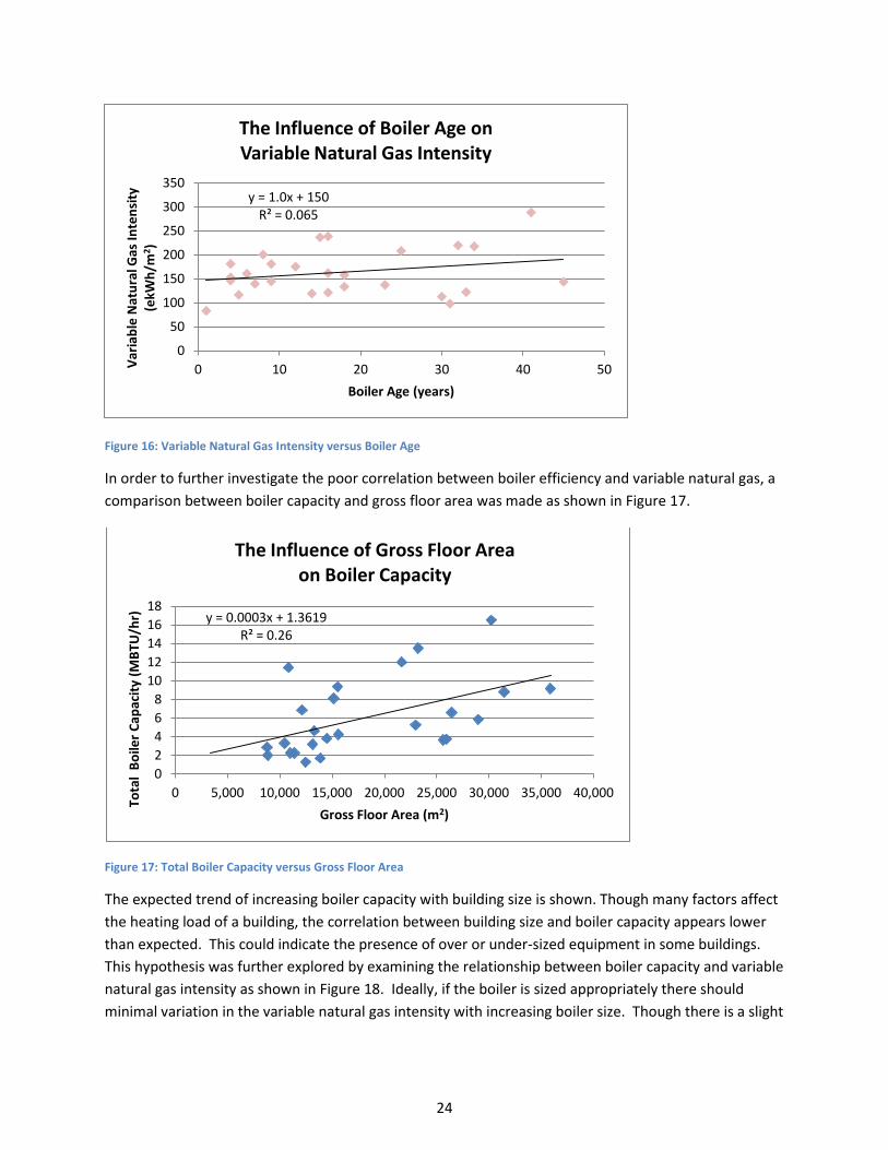
24
Figure 16: Variable Natural Gas Intensity versus Boiler Age
In order to further investigate the poor correlation between boiler efficiency and variable natural gas, a
comparison between boiler capacity and gross floor area was made as shown in Figure 17.
Figure 17: Total Boiler Capacity versus Gross Floor Area
The expected trend of increasing boiler capacity with building size is shown. Though many factors affect
the heating load of a building, the correlation between building size and boiler capacity appears lower
than expected. This could indicate the presence of over or under-sized equipment in some buildings.
This hypothesis was further explored by examining the relationship between boiler capacity and variable
natural gas intensity as shown in Figure 18. Ideally, if the boiler is sized appropriately there should
minimal variation in the variable natural gas intensity with increasing boiler size. Though there is a slight
y = 1.0x + 150 R² = 0.065
0
50
100
150
200
250
300
350
0 10 20 30 40 50 Var
iab
le N
atu
ral G
as In
ten
sity
(e
kWh
/m2 )
Boiler Age (years)
The Influence of Boiler Age on Variable Natural Gas Intensity
y = 0.0003x + 1.3619 R² = 0.26
0
2
4
6
8
10
12
14
16
18
0 5,000 10,000 15,000 20,000 25,000 30,000 35,000 40,000
Tota
l B
oile
r C
apac
ity
(MB
TU/h
r)
Gross Floor Area (m2)
The Influence of Gross Floor Area on Boiler Capacity
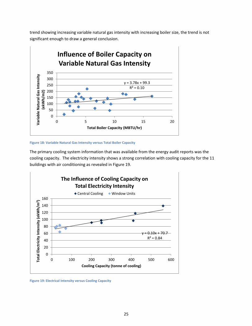
25
trend showing increasing variable natural gas intensity with increasing boiler size, the trend is not
significant enough to draw a general conclusion.
Figure 18: Variable Natural Gas Intensity versus Total Boiler Capacity
The primary cooling system information that was available from the energy audit reports was the
cooling capacity. The electricity intensity shows a strong correlation with cooling capacity for the 11
buildings with air conditioning as revealed in Figure 19.
Figure 19: Electrical Intensity versus Cooling Capacity
y = 3.78x + 99.3 R² = 0.10
0
50
100
150
200
250
300
350
0 5 10 15 20
Var
iab
le N
atu
ral G
as In
ten
sity
(e
kWh
/m2
)
Total Boiler Capacity (MBTU/hr)
Influence of Boiler Capacity on Variable Natural Gas Intensity
y = 0.10x + 70.7 R² = 0.84
0
20
40
60
80
100
120
140
160
0 100 200 300 400 500 600 Tota
l Ele
ctri
city
In
ten
sity
(e
kWh
/m2 )
Cooling Capacity (tonne of cooling)
The Influence of Cooling Capacity on Total Electricity Intensity
Central Cooling Window Units
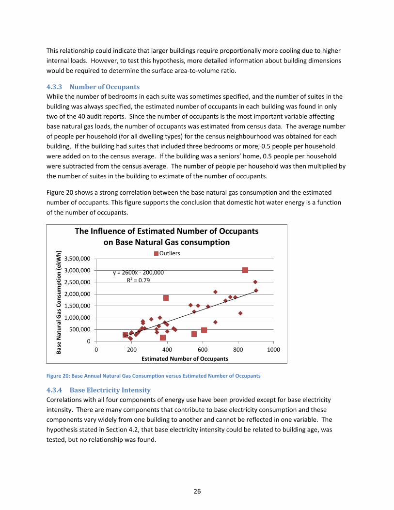
26
This relationship could indicate that larger buildings require proportionally more cooling due to higher
internal loads. However, to test this hypothesis, more detailed information about building dimensions
would be required to determine the surface area-to-volume ratio.
4.3.3 Number of Occupants
While the number of bedrooms in each suite was sometimes specified, and the number of suites in the
building was always specified, the estimated number of occupants in each building was found in only
two of the 40 audit reports. Since the number of occupants is the most important variable affecting
base natural gas loads, the number of occupants was estimated from census data. The average number
of people per household (for all dwelling types) for the census neighbourhood was obtained for each
building. If the building had suites that included three bedrooms or more, 0.5 people per household
were added on to the census average. If the building was a seniors’ home, 0.5 people per household
were subtracted from the census average. The number of people per household was then multiplied by
the number of suites in the building to estimate of the number of occupants.
Figure 20 shows a strong correlation between the base natural gas consumption and the estimated
number of occupants. This figure supports the conclusion that domestic hot water energy is a function
of the number of occupants.
Figure 20: Base Annual Natural Gas Consumption versus Estimated Number of Occupants
4.3.4 Base Electricity Intensity
Correlations with all four components of energy use have been provided except for base electricity
intensity. There are many components that contribute to base electricity consumption and these
components vary widely from one building to another and cannot be reflected in one variable. The
hypothesis stated in Section 4.2, that base electricity intensity could be related to building age, was
tested, but no relationship was found.
y = 2600x - 200,000 R² = 0.79
0
500,000
1,000,000
1,500,000
2,000,000
2,500,000
3,000,000
3,500,000
0 200 400 600 800 1000 Bas
e N
atu
ral G
as C
on
sum
pti
on
(e
kWh
)
Estimated Number of Occupants
The Influence of Estimated Number of Occupants on Base Natural Gas consumption
Outliers
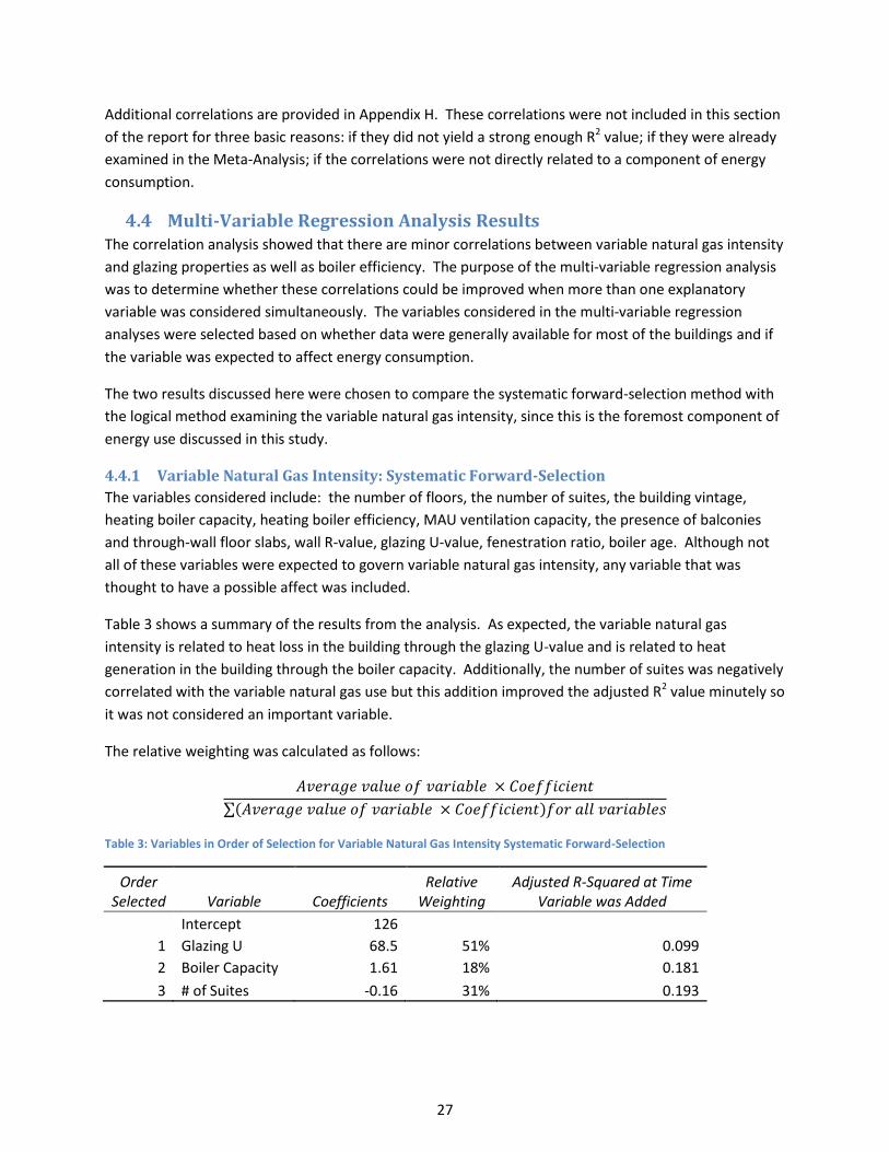
27
Additional correlations are provided in Appendix H. These correlations were not included in this section
of the report for three basic reasons: if they did not yield a strong enough R2 value; if they were already
examined in the Meta-Analysis; if the correlations were not directly related to a component of energy
consumption.
4.4 Multi-Variable Regression Analysis Results The correlation analysis showed that there are minor correlations between variable natural gas intensity
and glazing properties as well as boiler efficiency. The purpose of the multi-variable regression analysis
was to determine whether these correlations could be improved when more than one explanatory
variable was considered simultaneously. The variables considered in the multi-variable regression
analyses were selected based on whether data were generally available for most of the buildings and if
the variable was expected to affect energy consumption.
The two results discussed here were chosen to compare the systematic forward-selection method with
the logical method examining the variable natural gas intensity, since this is the foremost component of
energy use discussed in this study.
4.4.1 Variable Natural Gas Intensity: Systematic Forward-Selection
The variables considered include: the number of floors, the number of suites, the building vintage,
heating boiler capacity, heating boiler efficiency, MAU ventilation capacity, the presence of balconies
and through-wall floor slabs, wall R-value, glazing U-value, fenestration ratio, boiler age. Although not
all of these variables were expected to govern variable natural gas intensity, any variable that was
thought to have a possible affect was included.
Table 3 shows a summary of the results from the analysis. As expected, the variable natural gas
intensity is related to heat loss in the building through the glazing U-value and is related to heat
generation in the building through the boiler capacity. Additionally, the number of suites was negatively
correlated with the variable natural gas use but this addition improved the adjusted R2 value minutely so
it was not considered an important variable.
The relative weighting was calculated as follows:
Table 3: Variables in Order of Selection for Variable Natural Gas Intensity Systematic Forward-Selection
Order Selected Variable Coefficients
Relative Weighting
Adjusted R-Squared at Time Variable was Added
Intercept 126
1 Glazing U 68.5 51% 0.099
2 Boiler Capacity 1.61 18% 0.181
3 # of Suites -0.16 31% 0.193
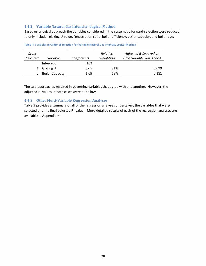
28
4.4.2 Variable Natural Gas Intensity: Logical Method
Based on a logical approach the variables considered in the systematic forward-selection were reduced
to only include: glazing U-value, fenestration ratio, boiler efficiency, boiler capacity, and boiler age.
Table 4: Variables in Order of Selection for Variable Natural Gas Intensity Logical Method
Order Selected Variable Coefficients
Relative Weighting
Adjusted R-Squared at Time Variable was Added
Intercept 102
1 Glazing U 67.5 81% 0.099
2 Boiler Capacity 1.09 19% 0.181
The two approaches resulted in governing variables that agree with one another. However, the
adjusted R2 values in both cases were quite low.
4.4.3 Other Multi-Variable Regression Analyses
Table 5 provides a summary of all of the regression analyses undertaken, the variables that were
selected and the final adjusted R2 value. More detailed results of each of the regression analyses are
available in Appendix H.
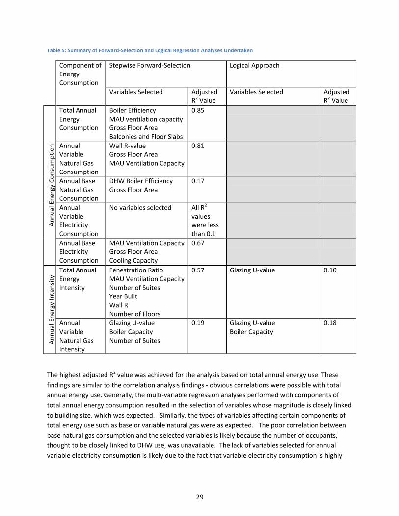
29
Table 5: Summary of Forward-Selection and Logical Regression Analyses Undertaken
Component of Energy Consumption
Stepwise Forward-Selection Logical Approach
Variables Selected Adjusted R2 Value
Variables Selected Adjusted R2 Value
An
nu
al E
ner
gy C
on
sum
pti
on
Total Annual Energy Consumption
Boiler Efficiency MAU ventilation capacity Gross Floor Area Balconies and Floor Slabs
0.85
Annual Variable Natural Gas Consumption
Wall R-value Gross Floor Area MAU Ventilation Capacity
0.81
Annual Base Natural Gas Consumption
DHW Boiler Efficiency Gross Floor Area
0.17
Annual Variable Electricity Consumption
No variables selected All R2 values were less than 0.1
Annual Base Electricity Consumption
MAU Ventilation Capacity Gross Floor Area Cooling Capacity
0.67
An
nu
al E
ner
gy In
ten
sity
Total Annual Energy Intensity
Fenestration Ratio MAU Ventilation Capacity Number of Suites Year Built Wall R Number of Floors
0.57 Glazing U-value 0.10
Annual Variable Natural Gas Intensity
Glazing U-value Boiler Capacity Number of Suites
0.19 Glazing U-value Boiler Capacity
0.18
The highest adjusted R2 value was achieved for the analysis based on total annual energy use. These
findings are similar to the correlation analysis findings - obvious correlations were possible with total
annual energy use. Generally, the multi-variable regression analyses performed with components of
total annual energy consumption resulted in the selection of variables whose magnitude is closely linked
to building size, which was expected. Similarly, the types of variables affecting certain components of
total energy use such as base or variable natural gas were as expected. The poor correlation between
base natural gas consumption and the selected variables is likely because the number of occupants,
thought to be closely linked to DHW use, was unavailable. The lack of variables selected for annual
variable electricity consumption is likely due to the fact that variable electricity consumption is highly
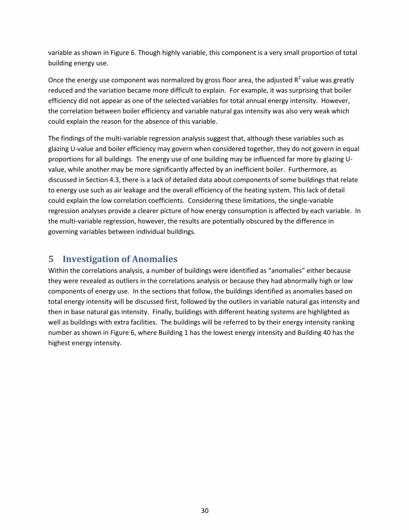
30
variable as shown in Figure 6. Though highly variable, this component is a very small proportion of total
building energy use.
Once the energy use component was normalized by gross floor area, the adjusted R2 value was greatly
reduced and the variation became more difficult to explain. For example, it was surprising that boiler
efficiency did not appear as one of the selected variables for total annual energy intensity. However,
the correlation between boiler efficiency and variable natural gas intensity was also very weak which
could explain the reason for the absence of this variable.
The findings of the multi-variable regression analysis suggest that, although these variables such as
glazing U-value and boiler efficiency may govern when considered together, they do not govern in equal
proportions for all buildings. The energy use of one building may be influenced far more by glazing U-
value, while another may be more significantly affected by an inefficient boiler. Furthermore, as
discussed in Section 4.3, there is a lack of detailed data about components of some buildings that relate
to energy use such as air leakage and the overall efficiency of the heating system. This lack of detail
could explain the low correlation coefficients. Considering these limitations, the single-variable
regression analyses provide a clearer picture of how energy consumption is affected by each variable. In
the multi-variable regression, however, the results are potentially obscured by the difference in
governing variables between individual buildings.
5 Investigation of Anomalies Within the correlations analysis, a number of buildings were identified as “anomalies” either because
they were revealed as outliers in the correlations analysis or because they had abnormally high or low
components of energy use. In the sections that follow, the buildings identified as anomalies based on
total energy intensity will be discussed first, followed by the outliers in variable natural gas intensity and
then in base natural gas intensity. Finally, buildings with different heating systems are highlighted as
well as buildings with extra facilities. The buildings will be referred to by their energy intensity ranking
number as shown in Figure 6, where Building 1 has the lowest energy intensity and Building 40 has the
highest energy intensity.
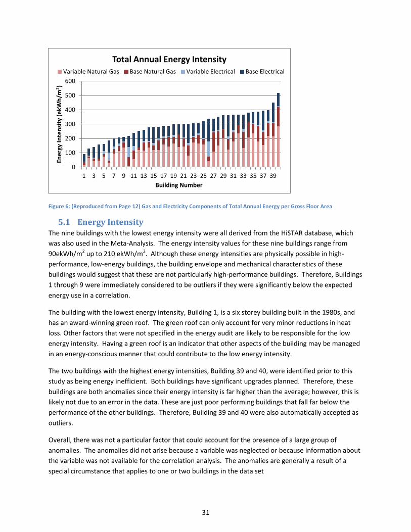
31
Figure 6: (Reproduced from Page 12) Gas and Electricity Components of Total Annual Energy per Gross Floor Area
5.1 Energy Intensity The nine buildings with the lowest energy intensity were all derived from the HiSTAR database, which
was also used in the Meta-Analysis. The energy intensity values for these nine buildings range from
90ekWh/m2 up to 210 ekWh/m2. Although these energy intensities are physically possible in high-
performance, low-energy buildings, the building envelope and mechanical characteristics of these
buildings would suggest that these are not particularly high-performance buildings. Therefore, Buildings
1 through 9 were immediately considered to be outliers if they were significantly below the expected
energy use in a correlation.
The building with the lowest energy intensity, Building 1, is a six storey building built in the 1980s, and
has an award-winning green roof. The green roof can only account for very minor reductions in heat
loss. Other factors that were not specified in the energy audit are likely to be responsible for the low
energy intensity. Having a green roof is an indicator that other aspects of the building may be managed
in an energy-conscious manner that could contribute to the low energy intensity.
The two buildings with the highest energy intensities, Building 39 and 40, were identified prior to this
study as being energy inefficient. Both buildings have significant upgrades planned. Therefore, these
buildings are both anomalies since their energy intensity is far higher than the average; however, this is
likely not due to an error in the data. These are just poor performing buildings that fall far below the
performance of the other buildings. Therefore, Building 39 and 40 were also automatically accepted as
outliers.
Overall, there was not a particular factor that could account for the presence of a large group of
anomalies. The anomalies did not arise because a variable was neglected or because information about
the variable was not available for the correlation analysis. The anomalies are generally a result of a
special circumstance that applies to one or two buildings in the data set
0
100
200
300
400
500
600
1 3 5 7 9 11 13 15 17 19 21 23 25 27 29 31 33 35 37 39
Ene
rgy
Inte
nsi
ty (
ekW
h/m
2 )
Building Number
Total Annual Energy Intensity Variable Natural Gas Base Natural Gas Variable Electrical Base Electrical
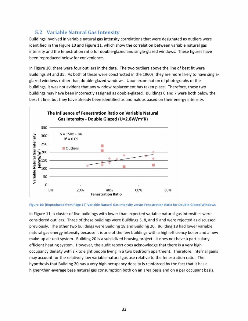
32
5.2 Variable Natural Gas Intensity Buildings involved in variable natural gas intensity correlations that were designated as outliers were
identified in the Figure 10 and Figure 11, which show the correlation between variable natural gas
intensity and the fenestration ratio for double-glazed and single-glazed windows. These figures have
been reproduced below for convenience.
In Figure 10, there were four outliers in the data. The two outliers above the line of best fit were
Buildings 34 and 35. As both of these were constructed in the 1960s, they are more likely to have single-
glazed windows rather than double-glazed windows. Upon examination of photographs of the
buildings, it was not evident that any window replacement has taken place. Therefore, these two
buildings may have been incorrectly assigned as double-glazed. Buildings 6 and 7 were both below the
best fit line, but they have already been identified as anomalous based on their energy intensity.
Figure 10: (Reproduced from Page 17) Variable Natural Gas Intensity versus Fenestration Ratio for Double-Glazed Windows
In Figure 11, a cluster of five buildings with lower than expected variable natural gas intensities were
considered outliers. Three of these buildings were Buildings 5, 8, and 9 and were rejected as discussed
previously. The other two buildings were Building 18 and Building 20. Building 18 had lower variable
natural gas energy intensity because it is one of the few buildings with a high efficiency boiler and a new
make-up air unit system. Building 20 is a subsidized housing project. It does not have a particularly
efficient heating system. However, the audit report does acknowledge that there is a very high
occupancy density with six to eight people living in a two bedroom apartment. Therefore, internal gains
may account for the relatively low variable natural gas use relative to the fenestration ratio. The
hypothesis that Building 20 has a very high occupancy density is reinforced by the fact that it has a
higher-than-average base natural gas consumption both on an area basis and on a per occupant basis.
y = 150x + 84 R² = 0.69
0
50
100
150
200
250
300
350
0% 20% 40% 60% 80%
Var
iab
le N
atu
ral G
as In
ten
sity
(e
kWh
/m2)
Fenestration Ratio
The Influence of Fenestration Ratio on Variable Natural Gas Intensity - Double Glazed (U=2.8W/m2K)
Outliers
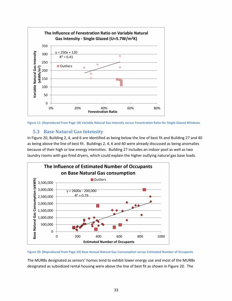
33
Figure 11: (Reproduced from Page 18) Variable Natural Gas Intensity versus Fenestration Ratio for Single-Glazed Windows
5.3 Base Natural Gas Intensity In Figure 20, Building 2, 4, and 6 are identified as being below the line of best fit and Building 27 and 40
as being above the line of best fit. Buildings 2, 4, 6 and 40 were already discussed as being anomalies
because of their high or low energy intensities. Building 27 includes an indoor pool as well as two
laundry rooms with gas-fired dryers, which could explain the higher outlying natural gas base loads.
Figure 20: (Reproduced from Page 24) Base Annual Natural Gas Consumption versus Estimated Number of Occupants
The MURBs designated as seniors’ homes tend to exhibit lower energy use and most of the MURBs
designated as subsidized rental housing were above the line of best fit as shown in Figure 20. The
y = 250x + 120 R² = 0.41
0
50
100
150
200
250
300
350
0% 20% 40% 60% 80%
Var
iab
le N
atu
ral G
as In
ten
sity
(e
kWh
/m2 )
Fenestration Ratio
The Influence of Fenestration Ratio on Variable Natural Gas Intensity - Single Glazed (U=5.7W/m2K)
Outliers
y = 2600x - 200,000 R² = 0.79
0
500,000
1,000,000
1,500,000
2,000,000
2,500,000
3,000,000
3,500,000
0 200 400 600 800 1000 Bas
e N
atu
ral G
as C
on
sum
pti
on
(e
kWh
)
Estimated Number of Occupants
The Influence of Estimated Number of Occupants on Base Natural Gas consumption
Outliers

34
reason for this trend is probably because the estimate of the number of occupants in the building was
not accurate. The number of occupants in each apartment is probably higher than the census average in
subsidized housing and below the census average in senior housing. An attempt to account for the
lower occupancy in seniors’ housing was made by subtracting 0.5 from the average number of people
per household leaving about 1.8 people per household for most neighborhoods where the seniors’
housing was located. In fact, the average number of people per household is probably just above one.
5.4 Alternative Heating Systems Buildings 10 and 11 had below average energy intensity and buildings 37 and 38 had above average
energy intensities. One of the reasons for this may have been because these buildings had a unique
aspect to their heating system compared with the other buildings in the data set.
Building 10 has a radiant heating system consisting of electrical resistance coils in the floor slabs.
Radiant heating systems are more efficient than other systems because radiant heating systems can
heat a room to a lower set point air temperature while allowing the occupants to still feel comfortable.
Since the indoor air is cooler, less heat is lost through air leakage and transmission through the building
envelope. Further, the building has also had new windows installed, which is an additional factor that
accounts for the building’s relatively low energy intensity since the new windows reduce the conductive
heat losses and losses through air leakage .
Building 11 does not have heating provided by a central boiler. Instead, each suite has a separate boiler
that provides domestic hot water and heating. This type of configuration can lead to reduced energy
use for a few reasons. First, less heat is wasted as it is being distributed from the boiler around the
building. Second, it is likely that occupants are billed individually for their hot water and heating so they
are more conscious of wasting hot water and have a motivation keep the thermostat at a lower
temperature. Finally, the smaller individual boilers may manage demand more efficiently than central
boiler that have to keep large quantities of water heated even if they are not being used.
In Buildings 37 and 38, the domestic hot water is generated by the heating boilers. Generally, this
configuration should be more efficient. However, in the case of Buildings 37 and 38, there are two large
heating boilers in each building which both have a much greater capacity than a domestic hot water
boiler would. Even with just one boiler running, the heating output could be much greater than
required and therefore, the heating system may be operating inefficiently and using more energy.
5.5 Additional Facilities Building 38 has the highest per suite energy use as shown in Figure 7. This is likely due to the fact that
the building contains a child care centre that is not accounted for separately in the energy bills.
Therefore, while the attributed suite size is large, this is because a significant portion of the building is
taken up by the child care centre. In combination with the inefficient domestic hot water system, the
child care centre may also contribute to the high energy intensity of Building 38.
Swimming pools included in the building facilities probably contribute to the above average energy
intensity in Buildings 29 and 39. Buildings 28, 29, 35 and 36 all have heated underground parking
35
garages that could contribute to their above average energy intensity. Since the parking garage has not
been included in the gross floor area for each of the buildings, any energy consumed by heating,
ventilation or lighting of the parking garage is added directly to the building energy use without any
differentiation that the energy is actually being consumed outside of the gross floor area.
6 Conclusions A number of important conclusions emerge from this study. This section includes conclusions regarding
the correlation between energy use and building characteristics. As well, a number of other important
findings that were not anticipated at the outset of this study are summarized here.
1) The average energy intensity of the buildings in this study was found to be 292ekWh/m2. This
finding is similar to the findings of the Meta-Analysis (295ekWh/m2). These energy intensities
were compared to a weighted average of various consumer-side studies of energy use in
Toronto and Ontario MURBs (305ekWh/m2). However, the data from these studies have not
been weather-normalized. It is interesting to note that there is a difference in MURB energy
intensities between supplier and consumer-side studies. The supplier-side studies were found
to be consistently lower than the consumer-side studies. The reason for the lower supply-side
values requires further investigation. Thus, when making a comparison between energy
intensity statistics, the data source must be identified in order to allow for direct comparison.
As the data in this study were collected directly from building utility bills, it is only appropriate
to compare the results to other consumer-side studies.
2) The average energy mix of the refined data set is 33% electricity and 67% natural gas which is
almost identical to the reported energy mix of apartment buildings in Ontario, 34% electricity
and 66% natural gas (NRCan, 2008).
3) Two variables related to the building envelope were tested for correlation with variable natural
gas and total electricity use: fenestration ratio and glazing U-value. The fenestration ratio was
shown to affect energy use related to heating and cooling as expected. The correlation was
shown to be stronger in buildings with double-glazed windows than in buildings with single-
glazed windows. The considerable variation in the data correlating the glazing U-value with
heating and cooling loads suggests that other window-related considerations are affecting
energy usage.
4) One hypothesis that may explain the weaker correlation between single-glazed windows and
variable natural gas and total electricity may be the underlying effects of air leakage around and
through operable windows. However, this hypothesis could not be tested since no data on the
air tightness of assemblies, and operable window air tightness in particular, were available.
Further, the division of windows into single-glazed and double-glazed categories may not
capture other underlying variables such as the overall U-value of the window. The overall glazing
U-value estimates were based on whether the windows were single- or double-glazed but the
36
estimates did not take into account the type of frame used. The type and proportion of frames
greatly affects the overall U-value of the windows since frames, particularly aluminum frames,
represent significant thermal bridges. Unfortunately, the data set did not contain particulars
concerning the type of window frames.
5) Boiler efficiencies were found to be weakly correlated with variable natural gas consumption.
This rather surprising finding can be explained in two ways. First, boiler efficiency estimates
reported in the data sets may be inaccurate. Secondly, boiler efficiency alone is not a sufficient
indicator of the overall level of heating system performance. An oversized heating system that
frequently cycles on and off may have a seasonal efficiency that is much lower than the rated
operating efficiency. It was also found that boiler age was poorly correlated with variable
natural gas use. This could be due to the approximate nature of the boiler age estimates or,
more likely, that boiler age is not a good proxy for heating system performance.
6) The number of occupants was shown to be the governing variable related to base natural gas
consumption as expected. However, this result was based on only an estimate of the number of
occupants from census data and could be refined with improvements in the estimate of the
actual number of occupants.
7) The analysis of anomalies revealed that there was not one particular factor that could explain a
large group of the anomalies. However, information on special facilities such as the existence of
a swimming pool or daycare facility included in the buildings aided in the explanation of a
number of the anomalies.
7 Recommendations This section contains recommendations concerning improving the quality and extent of building data.
Recommendations concerning the methods used to analyze and normalize data will be highlighted here
as well.
1) Throughout this study, the issue of data quality often arose. The refined data set that was
gathered for this report was an improvement on the data set used in the Meta-Analysis report.
The Refined Data set contained more complete energy consumption information and detailed
building characteristics for all of the buildings. As well, this data set more closely reflected the
population characteristics of mid- and high-rise MURBs in Toronto. Although the refined data
set was an improvement, there were still limitations in the building characteristics data for this
data set. The building characteristics data were collected by many different parties and
collection practices varied. This introduced inconsistencies in the data, which perhaps resulted
in the weaker-than-expected correlations such as those involving the fenestration ratio and the
boiler efficiency. Therefore, the authors recommend that a uniform data set template be
established with prescribed means of determining the necessary building variables.
37
2) Information about a number of building characteristics, such as estimates of envelope air
leakage, window and heating system details and number of occupants, thought to have a
potentially significant impact on energy use, should be included in the data set template. With a
more complete set of building characteristics, a truer picture of how energy is lost from these
buildings could be developed.
(i) Air leakage is commonly recognized as a significant source of heat loss. Due to a lack of
data, this study did not include a correlation between energy use and air leakage. With
air leakage test data and accompanying window characteristics collected (such as age
and condition including sealant condition), it may be possible to develop generalized air
leakage assumptions about certain window types (e.g. single, double, fixed, operable,
age windows and seals). Therefore, the authors recommend that air leakage
characteristics of various windows systems be quantified and incorporated into default
values in the database in the absence of specific blower door test data.
(ii) With respect to windows, information about the type of frame should be collected. An
estimate of the total heat loss associated with a typical window can be determined
using two-dimensional heat transfer calculation software provided information about
frame type, dimensions and glazing characteristics are known. As many of the windows
in MURBs are very similar, an on-line tool could be developed with the data from the
most common window types so that only dimensions would be required. This could aid
in retrofit decision-making by helping to determine whether window replacement is
required or if air sealing measures alone would provide sufficient energy savings.
(iii) With respect to heating systems, this study also found that boiler efficiency and age
estimates are not well correlated to variable natural gas use. This is reasonable because
there are many factors affecting heating system performance such as maintenance,
operation, controls, configuration and the appropriateness of the system size.
Therefore, the authors recommend that more information be collected about heating
system performance to determine if there is a way to estimate the aggregate effect of
these factors in order to quantify the impact on energy performance. Similar to testing
for air leakage, it may be necessary to conduct diagnostic tests on a number of boilers in
service to determine the natural gas input for heat output. Once again, after enough
have been tested, a correlation between one or more system characteristics such as
maintenance or operational practices and energy use could reveal what indicators
should be captured in an audit.
(iv) The number of occupants for each building was estimated using census data. The
authors recommend that the actual number of building occupants be collected during
an energy audit. This relatively easy step could be used to benchmark the efficiency of
the DHW system against other buildings given the seemingly high correlation with base
natural gas use.
38
(v) The presence of particular common area facilities was used to explain many of the
anomalous building energy findings. It is important to collect this type of information
during an audit. Therefore the authors recommend that information including area use,
square footage, lighting and equipment would be gathered. For underground parking
garages, the size, degree to which is it conditioned and presence of demand controlled
lighting or ventilation should be captured. However, if the parking garage energy use is
not included in the building energy bill, this information is unnecessary.
3) The energy intensities found in the Meta-Analysis and Refined Data set were normalized to the
Standard Weather Year or CWEC. The CWEC, developed by the National Research Council of
Canada, is based on data selected from a 30 year time span (Environment Canada and NRCan
2008). Using CWEC data resulted in a 20-30% increase in total annual energy consumption from
the actual building energy use data which ranged from 1998 to 2011. Other studies cited here
do not appear to have been weather normalized. Though normalizing to a standard weather
year is very important in order to make comparisons between different buildings and studies,
the challenge with using CWEC is that it overstates the actual energy intensity of the building
stock. When using this information to make assessments about the impact of energy retrofits,
the impacts of heating energy retrofits may be overstated while those affecting cooling loads
may be understated. Thus, using CWEC data as a normalization base may no longer be
appropriate for Toronto. Given this belief, the authors recommend that a new normalization
base be established that provides a more realistic estimate of energy savings.
4) The industry practice involves normalization by the conditioned floor area of the building to
allow for comparison of energy intensities between buildings of different sizes. The results from
this study agree with industry practice in that the relative standard error of the sample values
was reduced significantly by normalizing to gross floor area as opposed to number of suites.
Therefore, based on this finding, the authors recommend the continued use of normalizing
energy use data based on the gross conditioned floor area.
5) As discussed in Section 4.1, it was assumed that the area of the parking garage was not included
in the gross floor area of the building. However, sometimes this space is conditioned to some
degree and is therefore contributing to the heating load of the building. Regardless of whether
an underground parking area is conditioned, it can also contribute to the building electrical load
because of lighting and ventilation requirements. To include the area of this space in the gross
floor area would understate the energy intensity of the building but, by not including it,
buildings with conditioned parking garages would appear to have a higher energy intensity than
those with unconditioned parking areas. Ideally, parking garages should not be included in the
gross floor area calculations because they are often not conditioned to the same extent as the
rest of the building. However, if the energy use of this space is metered with the rest of the
building, the total annual energy use must be reduced before calculating the energy intensity of
the non-parking areas. Therefore, the authors recommend that parking garages and energy use

39
should be dealt with in a standard way. One way to accomplish this might be to determine
estimated energy use factors for each of energy end uses. For example the ENERGY STAR®
Portfolio Manager has established these factors for parking garage lighting and ventilation
(Energy Star, 2007) but heating load must also be taken into account. With this information it
may be possible to estimate the energy intensity of the parking garage and remove it from the
total building consumption.
8 Next Phase of This Study The analysis and conclusions from this report will be used to inform the final phase of the Energy Study.
The final phase will include three main parts:
- development of a database to organize MURB energy consumption data;
- generation of four detailed energy models to explore the projected benefits of a range of energy
retrofit options;
- suggestion of policy changes to encourage implementation of the most promising retrofit
measures.
The MURB energy consumption database will contain the 40 buildings in this report and have the
flexibility to include new buildings as data becomes available. By allowing for expansion, the analyses
and results presented here can be strengthened. The database will also provide built-in data processing
to ensure the same method for weather normalization, determination of base and variable loads, and
groupings for the type of building heating system are maintained.
A preliminary selection of the four buildings for which energy models will be generated has been made.
The buildings will represent the four main building vintage groups of 1960-1969, 1970-1979, 1980-1995,
and 1996-2010. Energy models for each building will be calibrated with actual energy consumption.
Then, a series of retrofit measures will be modeled on each building and the effects of these retrofits on
energy use explored.
Finally, suggestions will be made with respect to policy in order to encourage greater uptake of the
retrofit measures exhibiting the largest projected energy savings.
This study forms an important first step in determining actual baseline energy intensities of MURBs and
trends in building typologies. The final phase of the Energy Study is needed to make specific suggestions
based on the conclusions of this report.

40
9 References Arup. Community energy plan for pilot sites.[Online] Available:
http://www.toronto.ca/city_manager/pdf/tr_arup_cep.pdf Toronto: Mayor’s Tower Renewal, 2010.
Canada Mortgage and Housing Corporation. Analysis of the Annual Energy and Water Consumption of
Apartment Buildings in the CMHC HiSTAR Database. (Technical Series 01-142) [Online] Available:
http://www.cmhc.ca/publications/en/rh-pr/tech/01-142e.pdf, 2001.
City of Toronto and Statistics Canada. Release of 2006 census results marital status, families, households
and dwelling characteristics. [Online] Available:
http://www.toronto.ca/demographics/pdf/2006_families-households_backgrounder.pdf, 2007.
City of Toronto and Statistics Canada. 2011 census: population and dwelling counts. [Online] Available:
http://www.toronto.ca/demographics/pdf/2011-census-backgrounder.pdf, 2012.
Elmahdy, A. H., Building Research Note: Annual Consumption Data on Apartment Buildings. Division of Building Research, National Research Council of Canada. [Online] Available: http://www.nrc-cnrc.gc.ca/obj/irc/doc/pubs/brn/brn181/brn181.pdf, 1982.
Energy Star. ENERGY STAR® Performance Ratings Technical Methodology for Parking. [Online] Available:
http://www.energystar.gov/ia/business/evaluate_performance/parking_tech_desc.pdf, 2007.
Enermodal Engineering Limited. Review of OHC Building Energy and Water Audits. Technical Series 00-
110, Research Highlights Canadian Mortgage and Housing Corporation. [Online]
Available:http://cmhc.ca/odpub/pdf/62587.pdf?lang=en, 2000.
Environment Canada and the National Research Council of Canada. Canadian Weather for Energy
Calculations Updated User’s Manual. [Online] Available:
ftp://arcdm20.tor.ec.gc.ca/pub/dist/climate/CWEEDS_2005/ZIPPED%20FILES/ENGLISH/CWEEDS%20doc
umentation_Release9.txt, 2008.
Environment Canada. National Inventory Report 1990-2008. [Online] Available:
http://www.ec.gc.ca/Publications/default.asp?lang=En&xml=492D914C-2EAB-47AB-A045-
C62B2CDACC29. 2010
Environment Canada. National Inventory Report 1990-2010. [Online] Available:
http://www.ec.gc.ca/publications/default.asp?lang=En&xml=A91164E0-7CEB-4D61-841C-
BEA8BAA223F9. 2012
Hart, D. Energy and Water Consumption Load Profiles in Multi-Unit Residential Buildings (2005)
Technical Series 05-119, Research Highlights Canadian Mortgage and Housing Corporation, 2,
<http://www.cmhc-schl.gc.ca/odpub/pdf/64940.pdf> at 22 July 2012.
Hutcheon, N.B. and Handegord, G.O.P, Building Science for a Cold Climate, Institute for Research in
Construction, 1995.

41
Liu, R. Energy Consumption and Energy Intensity in Multi-unit Residential Buildings (MURBs) in Canada.
Canadian Building Energy End-Use Data and Analysis Centre. [Online]. Available:
http://www.cbeedac.com/publications/documents/MURBsrp04.pdf, 2007.
Natural Resources Canada, Survey of Household Energy Use 2003 Detailed Statistical Report. Office of
Energy Efficiency, [Online] Available:
http://oee.nrcan.gc.ca/Publications/statistics/sheu03/pdf/sheu03.pdf. 2006
Natural Resources Canada, Table 38: Apartments Secondary Energy Use and GHG Emissions by Energy
Source, 2008.
Natural Resources Canada, Survey of Household Energy Use 2007 Detailed Statistical Report. Office of
Energy Efficiency. [Online] Available:
http://oee.nrcan.gc.ca/publications/statistics/sheu07/pdf/sheu07.pdf 2010
Natural Resources Canada, Comprehensive Energy Use Database – Residential Sector. Office of Energy
Efficiency. [Online] Available;
http://oee.nrcan.gc.ca/corporate/statistics/neud/dpa/tablestrends2/res_ca_45_e_4.cfm?attr=0. 2012.
Natural Resources Canada, Energy Use Data Handbook Table 4. Office of Energy Efficiency. [Online]
Available:
http://oee.nrcan.gc.ca/corporate/statistics/neud/dpa/tableshandbook2/res_00_4_e_5.cfm?attr=0.
2012.
Stewart, G. and Thorne, J., Tower neighbourhood renewal in the greater golden horseshoe: An analysis
of high-rise tower apartment neighbourhoods developed in the post-war boom (1946-1984). [Online]
Available: http://www.cugr.ca/tnrggh. Toronto: University of Toronto, 2010.
TObuilt. A database of buildings in Toronto Canada. [Online] Available: http://www.tobuilt.ca/., 2012.
Tzekova, E., Pressnail, K.D., De Rose, D., Day, K., Evaluating the effectiveness of energy-efficient retrofits
on multi-unit residential buildings: two case studies. Winnipeg: 13th Canadian conference on buildings
science and technology, 2011.
10 Bibliography Environment Canada. National Climate Data and Information Archive. [Online]. Available:
http://www.climate.weatheroffice.gc.ca/Welcome_e.html, 2011.
Numerical Logics, Inc. Climate Information. [Online]. Available: http://www.numlog.ca/climate.html,
2011.
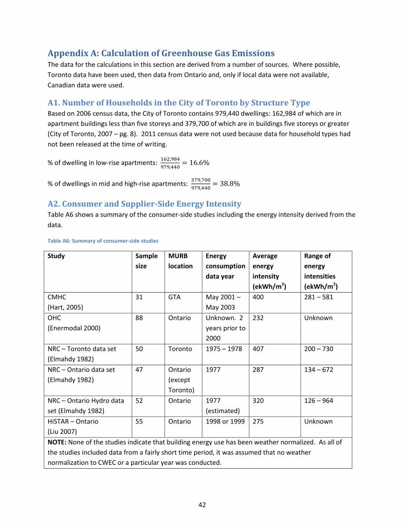
42
Appendix A: Calculation of Greenhouse Gas Emissions The data for the calculations in this section are derived from a number of sources. Where possible,
Toronto data have been used, then data from Ontario and, only if local data were not available,
Canadian data were used.
A1. Number of Households in the City of Toronto by Structure Type Based on 2006 census data, the City of Toronto contains 979,440 dwellings: 162,984 of which are in
apartment buildings less than five storeys and 379,700 of which are in buildings five storeys or greater
(City of Toronto, 2007 – pg. 8). 2011 census data were not used because data for household types had
not been released at the time of writing.
% of dwelling in low-rise apartments:
% of dwellings in mid and high-rise apartments:
A2. Consumer and Supplier-Side Energy Intensity Table A6 shows a summary of the consumer-side studies including the energy intensity derived from the
data.
Table A6: Summary of consumer-side studies
Study Sample
size
MURB
location
Energy
consumption
data year
Average
energy
intensity
(ekWh/m2)
Range of
energy
intensities
(ekWh/m2)
CMHC
(Hart, 2005)
31 GTA May 2001 –
May 2003
400 281 – 581
OHC
(Enermodal 2000)
88 Ontario Unknown. 2
years prior to
2000
232 Unknown
NRC – Toronto data set
(Elmahdy 1982)
50 Toronto 1975 – 1978 407 200 – 730
NRC – Ontario data set
(Elmahdy 1982)
47 Ontario
(except
Toronto)
1977 287 134 – 672
NRC – Ontario Hydro data
set (Elmahdy 1982)
52 Ontario 1977
(estimated)
320 126 – 964
HiSTAR – Ontario
(Liu 2007)
55 Ontario 1998 or 1999 275 Unknown
NOTE: None of the studies indicate that building energy use has been weather normalized. As all of
the studies included data from a fairly short time period, it was assumed that no weather
normalization to CWEC or a particular year was conducted.
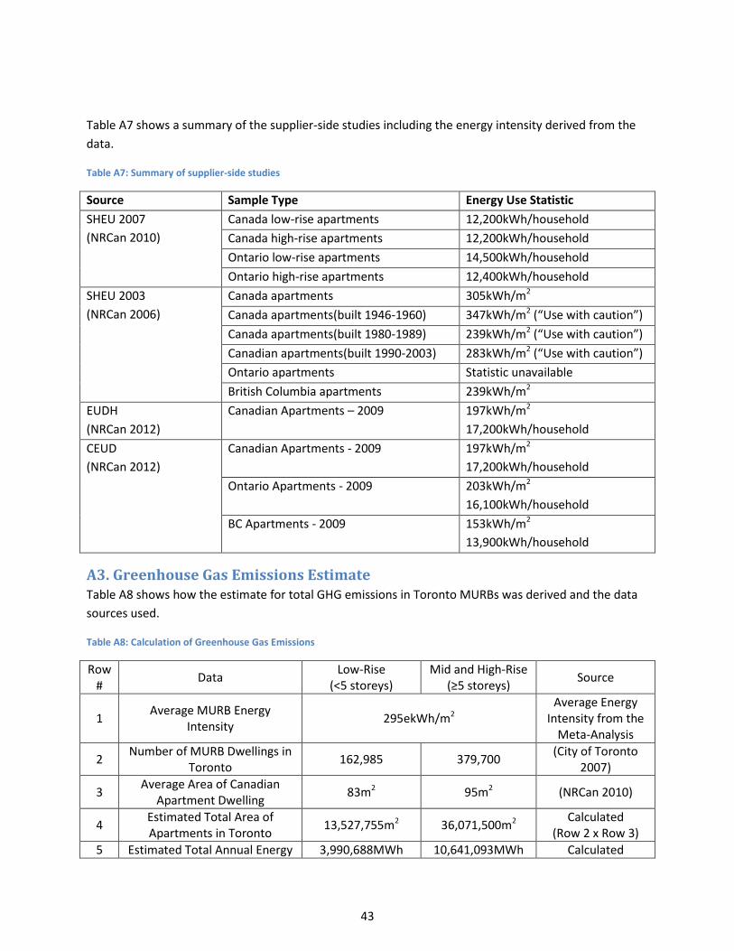
43
Table A7 shows a summary of the supplier-side studies including the energy intensity derived from the
data.
Table A7: Summary of supplier-side studies
Source Sample Type Energy Use Statistic
SHEU 2007
(NRCan 2010)
Canada low-rise apartments 12,200kWh/household
Canada high-rise apartments 12,200kWh/household
Ontario low-rise apartments 14,500kWh/household
Ontario high-rise apartments 12,400kWh/household
SHEU 2003
(NRCan 2006)
Canada apartments 305kWh/m2
Canada apartments(built 1946-1960) 347kWh/m2 (“Use with caution”)
Canada apartments(built 1980-1989) 239kWh/m2 (“Use with caution”)
Canadian apartments(built 1990-2003) 283kWh/m2 (“Use with caution”)
Ontario apartments Statistic unavailable
British Columbia apartments 239kWh/m2
EUDH
(NRCan 2012)
Canadian Apartments – 2009 197kWh/m2
17,200kWh/household
CEUD
(NRCan 2012)
Canadian Apartments - 2009 197kWh/m2
17,200kWh/household
Ontario Apartments - 2009 203kWh/m2
16,100kWh/household
BC Apartments - 2009 153kWh/m2
13,900kWh/household
A3. Greenhouse Gas Emissions Estimate Table A8 shows how the estimate for total GHG emissions in Toronto MURBs was derived and the data
sources used.
Table A8: Calculation of Greenhouse Gas Emissions
Row #
Data Low-Rise
(<5 storeys) Mid and High-Rise
(≥5 storeys) Source
1 Average MURB Energy
Intensity 295ekWh/m2
Average Energy Intensity from the
Meta-Analysis
2 Number of MURB Dwellings in
Toronto 162,985 379,700
(City of Toronto 2007)
3 Average Area of Canadian
Apartment Dwelling 83m2 95m2 (NRCan 2010)
4 Estimated Total Area of Apartments in Toronto
13,527,755m2 36,071,500m2 Calculated
(Row 2 x Row 3)
5 Estimated Total Annual Energy 3,990,688MWh 10,641,093MWh Calculated
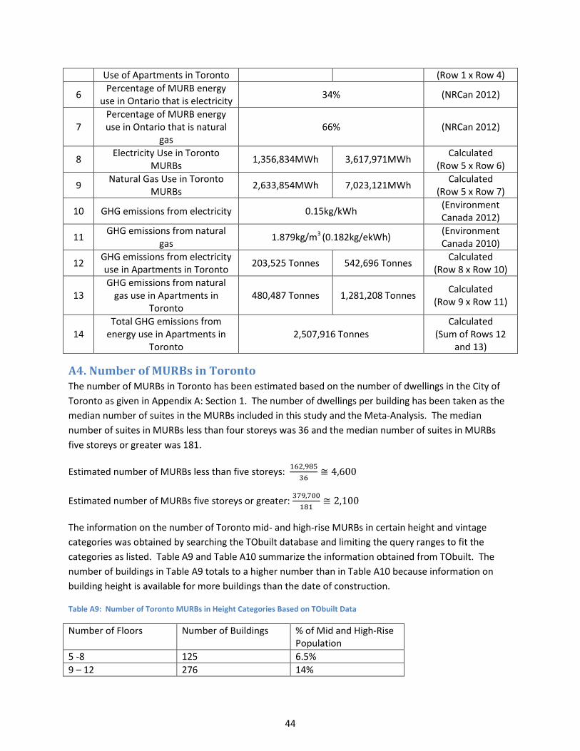
44
Use of Apartments in Toronto (Row 1 x Row 4)
6 Percentage of MURB energy
use in Ontario that is electricity 34% (NRCan 2012)
7 Percentage of MURB energy use in Ontario that is natural
gas 66% (NRCan 2012)
8 Electricity Use in Toronto
MURBs 1,356,834MWh 3,617,971MWh
Calculated (Row 5 x Row 6)
9 Natural Gas Use in Toronto
MURBs 2,633,854MWh 7,023,121MWh
Calculated (Row 5 x Row 7)
10 GHG emissions from electricity 0.15kg/kWh (Environment Canada 2012)
11 GHG emissions from natural
gas 1.879kg/m3 (0.182kg/ekWh)
(Environment Canada 2010)
12 GHG emissions from electricity use in Apartments in Toronto
203,525 Tonnes 542,696 Tonnes Calculated
(Row 8 x Row 10)
13 GHG emissions from natural
gas use in Apartments in Toronto
480,487 Tonnes 1,281,208 Tonnes Calculated
(Row 9 x Row 11)
14 Total GHG emissions from
energy use in Apartments in Toronto
2,507,916 Tonnes Calculated
(Sum of Rows 12 and 13)
A4. Number of MURBs in Toronto The number of MURBs in Toronto has been estimated based on the number of dwellings in the City of
Toronto as given in Appendix A: Section 1. The number of dwellings per building has been taken as the
median number of suites in the MURBs included in this study and the Meta-Analysis. The median
number of suites in MURBs less than four storeys was 36 and the median number of suites in MURBs
five storeys or greater was 181.
Estimated number of MURBs less than five storeys:
Estimated number of MURBs five storeys or greater:
The information on the number of Toronto mid- and high-rise MURBs in certain height and vintage
categories was obtained by searching the TObuilt database and limiting the query ranges to fit the
categories as listed. Table A9 and Table A10 summarize the information obtained from TObuilt. The
number of buildings in Table A9 totals to a higher number than in Table A10 because information on
building height is available for more buildings than the date of construction.
Table A9: Number of Toronto MURBs in Height Categories Based on TObuilt Data
Number of Floors Number of Buildings % of Mid and High-Rise Population
5 -8 125 6.5%
9 – 12 276 14%
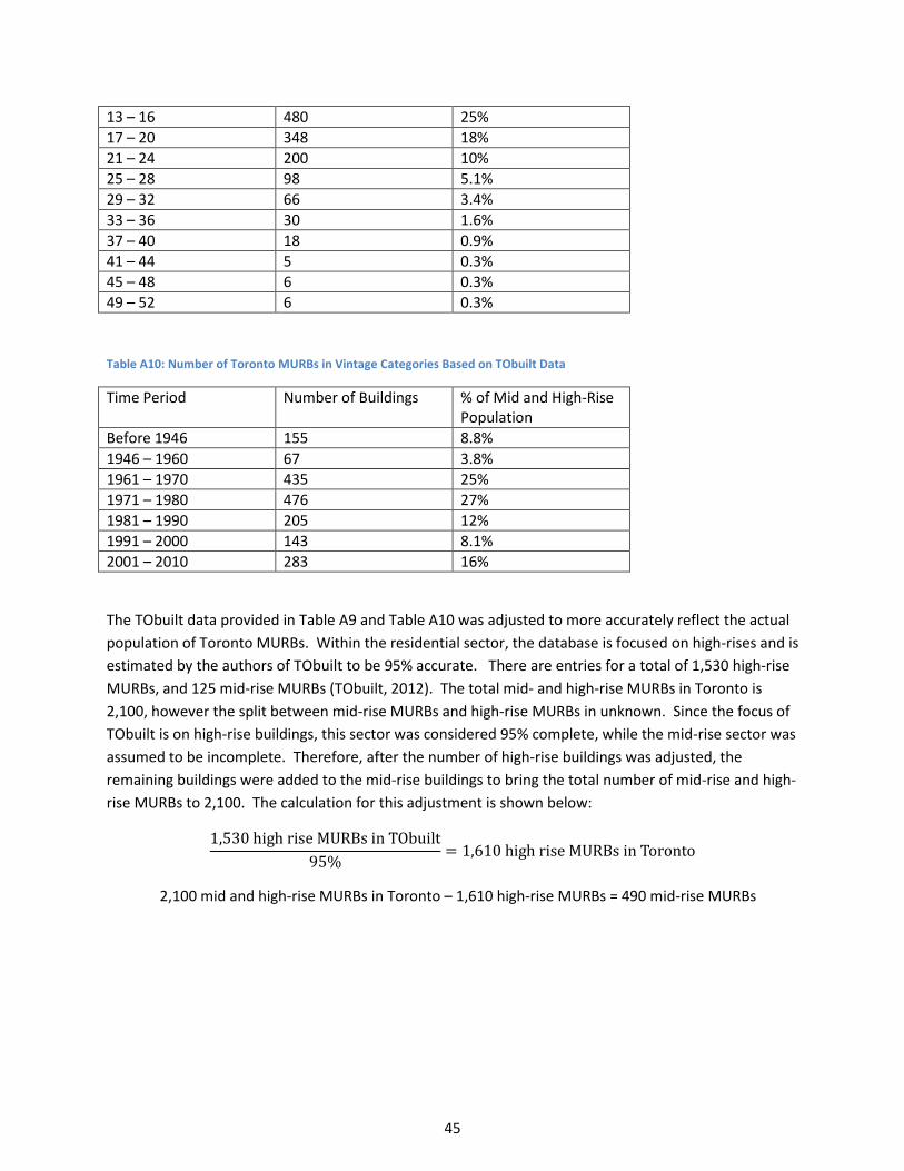
45
13 – 16 480 25%
17 – 20 348 18%
21 – 24 200 10%
25 – 28 98 5.1%
29 – 32 66 3.4%
33 – 36 30 1.6%
37 – 40 18 0.9%
41 – 44 5 0.3%
45 – 48 6 0.3%
49 – 52 6 0.3%
Table A10: Number of Toronto MURBs in Vintage Categories Based on TObuilt Data
Time Period Number of Buildings % of Mid and High-Rise Population
Before 1946 155 8.8%
1946 – 1960 67 3.8%
1961 – 1970 435 25%
1971 – 1980 476 27%
1981 – 1990 205 12%
1991 – 2000 143 8.1%
2001 – 2010 283 16%
The TObuilt data provided in Table A9 and Table A10 was adjusted to more accurately reflect the actual
population of Toronto MURBs. Within the residential sector, the database is focused on high-rises and is
estimated by the authors of TObuilt to be 95% accurate. There are entries for a total of 1,530 high-rise
MURBs, and 125 mid-rise MURBs (TObuilt, 2012). The total mid- and high-rise MURBs in Toronto is
2,100, however the split between mid-rise MURBs and high-rise MURBs in unknown. Since the focus of
TObuilt is on high-rise buildings, this sector was considered 95% complete, while the mid-rise sector was
assumed to be incomplete. Therefore, after the number of high-rise buildings was adjusted, the
remaining buildings were added to the mid-rise buildings to bring the total number of mid-rise and high-
rise MURBs to 2,100. The calculation for this adjustment is shown below:
2,100 mid and high-rise MURBs in Toronto – 1,610 high-rise MURBs = 490 mid-rise MURBs

46
Appendix B: Sample Letter of Request and FAQ Sheet Appendix B contains a copy of the letter that was sent to building owners during the data collection
process as well as the FAQs sheet sent later in the data acquisition process.

47
35 St. George Street
Toronto, ON, M5S 1A4
January 27, 2012
Subject: REQUEST FOR ELECTRICITY DATA
<<CONTACT NAME>>
<<BUILDING ADDRESS>>
Dear <<CONTACT NAME>>,
The Sustainable Building Group at the University of Toronto is working with the Toronto Atmospheric Fund to
develop a better understanding of energy use in multi-unit residential buildings (MURBs).
As part of the Green Condo Champions initiative, members of your board participated in training and engagement
programs focused on cutting energy costs and reducing greenhouse gas emissions and received an audit report
and recommendations for strategies to reduce the energy use in your building. These audit reports, used
anonymously, have been invaluable in establishing the foundations of a comprehensive MURB database that will
help inform policy makers and direct energy retrofit efforts.
To complete the data set, we are requesting access to your historical electricity records in order to match these
data with the existing natural gas data in the audit report. The anonymity of all of your energy performance data
will be strictly maintained. When entered into the energy use database, your building name and/or address will be
replaced with a unique number for the data analysis procedures.
Following completion of the study in September 2012, you will be provided with a ranking of your building within
the rest of the data set to determine your building’s level of energy performance compared to other similar
buildings.
Kindly complete both pages of the attached letter and return it in the self-addressed stamped envelope at your
earliest convenience. If you have any questions or concerns, please do not hesitate to contact me at
[email protected] or (416) 432-1535.
Your prompt attention and cooperation are greatly appreciated!
Kind Regards,
Clarissa Binkley
Sustainable Building Group Researcher
University of Toronto
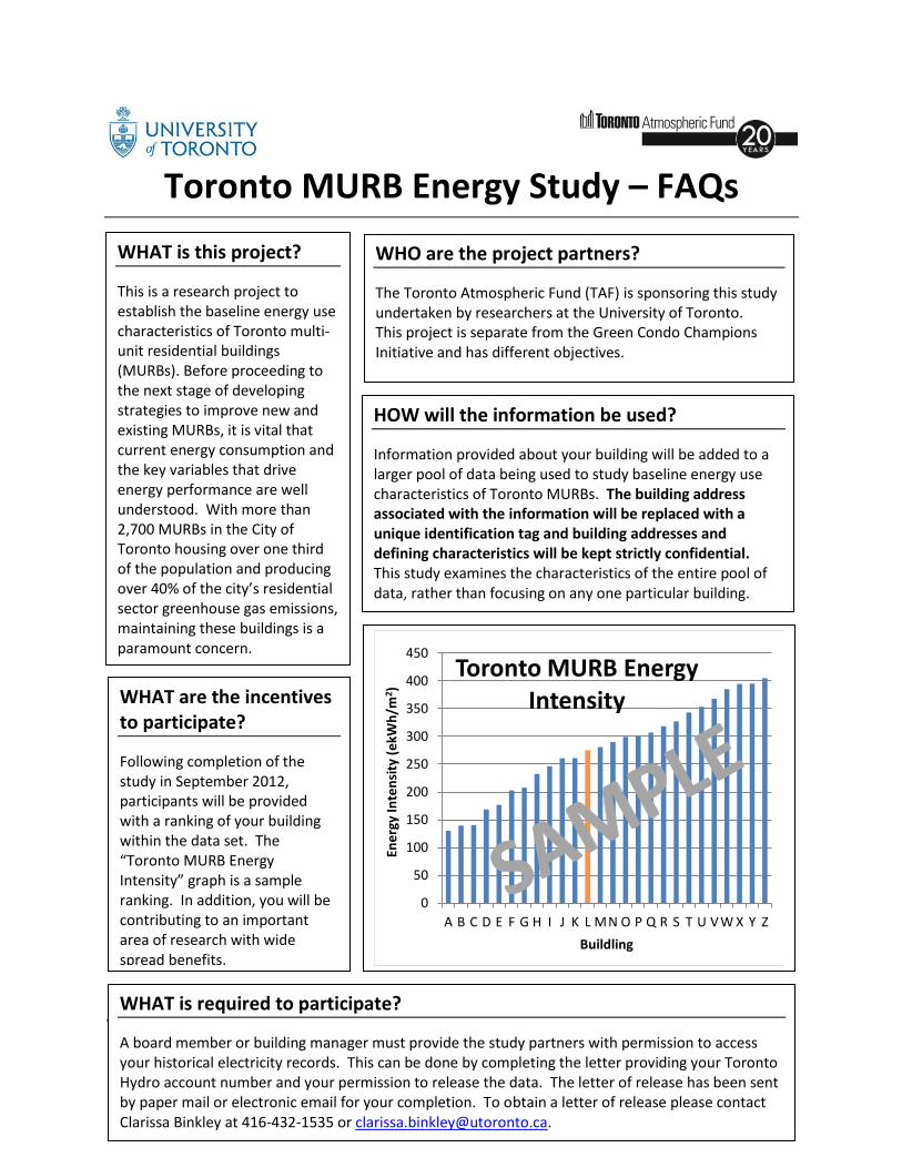
48
Toronto MURB Energy Study – FAQs
A
WHAT is this project?
This is a research project to establish the baseline energy use characteristics of Toronto multi-unit residential buildings (MURBs). Before proceeding to the next stage of developing strategies to improve new and existing MURBs, it is vital that current energy consumption and the key variables that drive energy performance are well understood. With more than 2,700 MURBs in the City of Toronto housing over one third of the population and producing over 40% of the city’s residential sector greenhouse gas emissions, maintaining these buildings is a paramount concern.
WHO are the project partners?
The Toronto Atmospheric Fund (TAF) is sponsoring this study undertaken by researchers at the University of Toronto. This project is separate from the Green Condo Champions Initiative and has different objectives.
HOW will the information be used?
Information provided about your building will be added to a larger pool of data being used to study baseline energy use characteristics of Toronto MURBs. The building address associated with the information will be replaced with a unique identification tag and building addresses and defining characteristics will be kept strictly confidential. This study examines the characteristics of the entire pool of data, rather than focusing on any one particular building.
WHAT are the incentives to participate?
Following completion of the study in September 2012, participants will be provided with a ranking of your building within the data set. The “Toronto MURB Energy Intensity” graph is a sample ranking. In addition, you will be contributing to an important area of research with wide spread benefits.
WHAT is required to participate?
A board member or building manager must provide the study partners with permission to access your historical electricity records. This can be done by completing the letter providing your Toronto Hydro account number and your permission to release the data. The letter of release has been sent by paper mail or electronic email for your completion. To obtain a letter of release please contact Clarissa Binkley at 416-432-1535 or [email protected].
0
50
100
150
200
250
300
350
400
450
A B C D E F G H I J K L M N O P Q R S T U V W X Y Z
Ene
rgy
Inte
nsi
ty (
ekW
h/m
2)
Buildling
Toronto MURB Energy Intensity
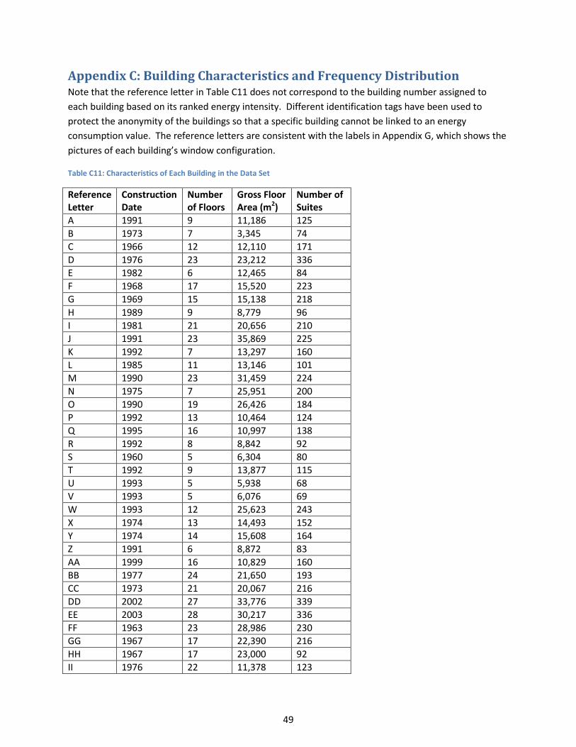
49
Appendix C: Building Characteristics and Frequency Distribution Note that the reference letter in Table C11 does not correspond to the building number assigned to
each building based on its ranked energy intensity. Different identification tags have been used to
protect the anonymity of the buildings so that a specific building cannot be linked to an energy
consumption value. The reference letters are consistent with the labels in Appendix G, which shows the
pictures of each building’s window configuration.
Table C11: Characteristics of Each Building in the Data Set
Reference Letter
Construction Date
Number of Floors
Gross Floor Area (m2)
Number of Suites
A 1991 9 11,186 125
B 1973 7 3,345 74
C 1966 12 12,110 171
D 1976 23 23,212 336
E 1982 6 12,465 84
F 1968 17 15,520 223
G 1969 15 15,138 218
H 1989 9 8,779 96
I 1981 21 20,656 210
J 1991 23 35,869 225
K 1992 7 13,297 160
L 1985 11 13,146 101
M 1990 23 31,459 224
N 1975 7 25,951 200
O 1990 19 26,426 184
P 1992 13 10,464 124
Q 1995 16 10,997 138
R 1992 8 8,842 92
S 1960 5 6,304 80
T 1992 9 13,877 115
U 1993 5 5,938 68
V 1993 5 6,076 69
W 1993 12 25,623 243
X 1974 13 14,493 152
Y 1974 14 15,608 164
Z 1991 6 8,872 83
AA 1999 16 10,829 160
BB 1977 24 21,650 193
CC 1973 21 20,067 216
DD 2002 27 33,776 339
EE 2003 28 30,217 336
FF 1963 23 28,986 230
GG 1967 17 22,390 216
HH 1967 17 23,000 92
II 1976 22 11,378 123
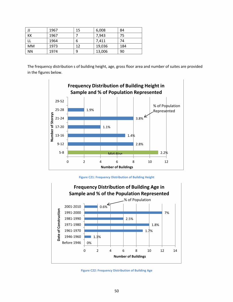
50
JJ 1967 15 6,008 84
KK 1967 7 7,943 75
LL 1964 6 7,411 74
MM 1973 12 19,036 184
NN 1974 9 13,006 90
The frequency distribution s of building height, age, gross floor area and number of suites are provided
in the figures below.
Figure C21: Frequency Distribution of Building Height
Figure C22: Frequency Distribution of Building Age
2.2%
2.8%
1.4%
1.1%
3.8%
1.9%
0 2 4 6 8 10 12
5-8
9-12
13-16
17-20
21-24
25-28
29-52
Number of Buildings
Nu
mb
er
of
Sto
reys
Frequency Distribution of Building Height in Sample and % of Population Represented
% of Population Represented
Mid-Rise
0%
1.3%
1.7%
1.8%
2.5%
7%
0.6%
0 2 4 6 8 10 12 14
Before 1946
1946-1960
1961-1970
1971-1980
1981-1990
1991-2000
2001-2010
Number of Buildings
Dat
e o
f C
on
stru
ctio
n
Frequency Distribution of Building Age in Sample and % of the Population Represented
% of Population
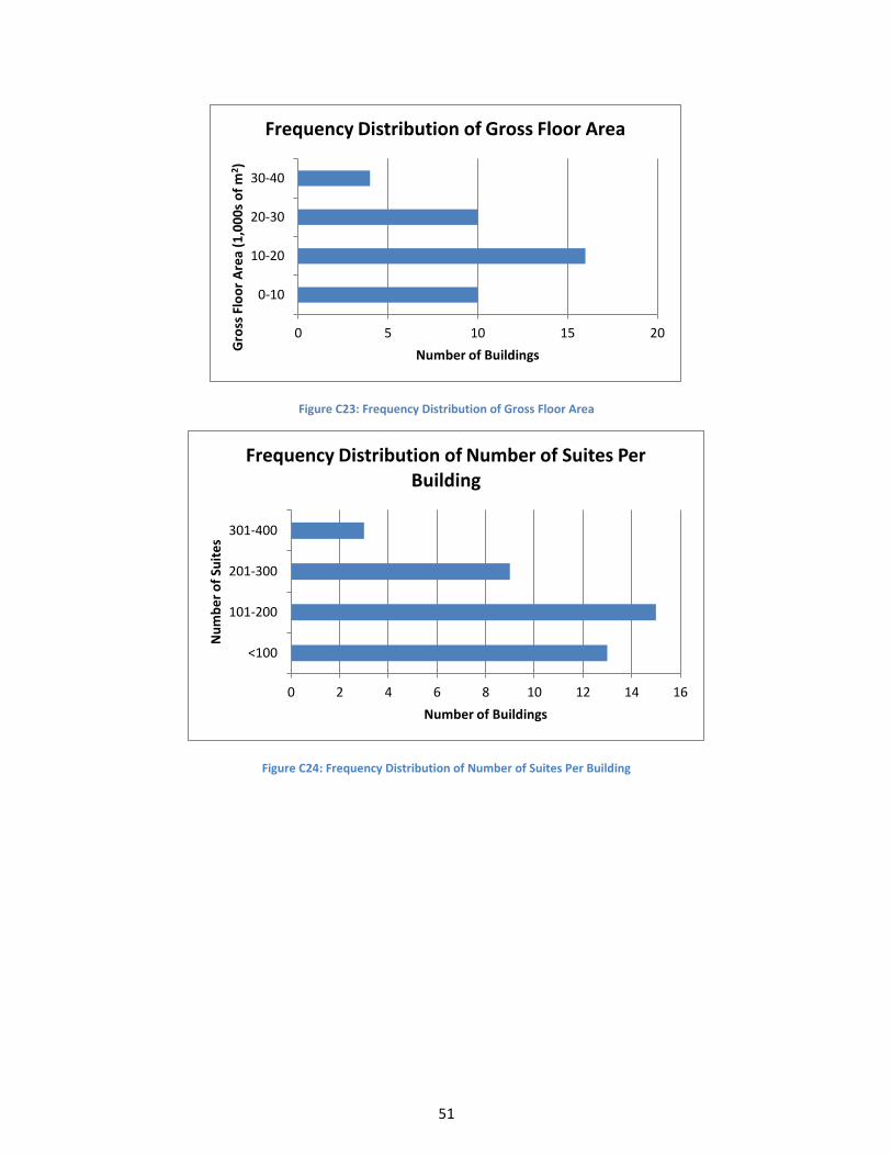
51
Figure C23: Frequency Distribution of Gross Floor Area
Figure C24: Frequency Distribution of Number of Suites Per Building
0 5 10 15 20
0-10
10-20
20-30
30-40
Number of Buildings
Gro
ss F
loo
r A
rea
(1,0
00
s o
f m
2 )
Frequency Distribution of Gross Floor Area
0 2 4 6 8 10 12 14 16
<100
101-200
201-300
301-400
Number of Buildings
Nu
mb
er
of
Suit
es
Frequency Distribution of Number of Suites Per Building
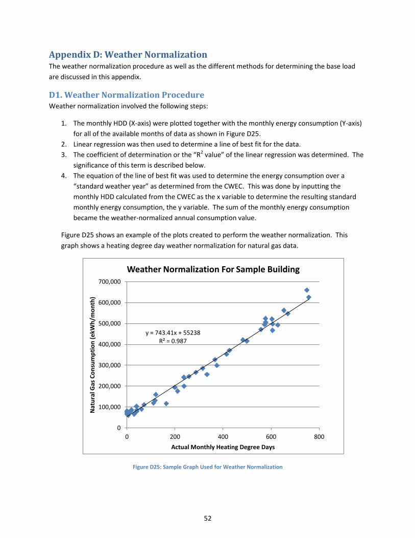
52
Appendix D: Weather Normalization The weather normalization procedure as well as the different methods for determining the base load
are discussed in this appendix.
D1. Weather Normalization Procedure Weather normalization involved the following steps:
1. The monthly HDD (X-axis) were plotted together with the monthly energy consumption (Y-axis)
for all of the available months of data as shown in Figure D25.
2. Linear regression was then used to determine a line of best fit for the data.
3. The coefficient of determination or the “R2 value” of the linear regression was determined. The
significance of this term is described below.
4. The equation of the line of best fit was used to determine the energy consumption over a
“standard weather year” as determined from the CWEC. This was done by inputting the
monthly HDD calculated from the CWEC as the x variable to determine the resulting standard
monthly energy consumption, the y variable. The sum of the monthly energy consumption
became the weather-normalized annual consumption value.
Figure D25 shows an example of the plots created to perform the weather normalization. This
graph shows a heating degree day weather normalization for natural gas data.
Figure D25: Sample Graph Used for Weather Normalization
y = 743.41x + 55238 R² = 0.987
0
100,000
200,000
300,000
400,000
500,000
600,000
700,000
0 200 400 600 800
Nat
ura
l Gas
Co
nsu
mp
tio
n (
ekW
h/m
on
th)
Actual Monthly Heating Degree Days
Weather Normalization For Sample Building

53
Historical weather data were retrieved and associated with the energy consumption data. Monthly HDD
and cooling degree day (CDD) data were obtained from Environment Canada for Toronto.
The energy consumption data associated with this weather data were then normalized to HDD data
using CWEC data, a ‘standard year’ of weather data provided by Environment Canada. A standard
reference year such as this captures average weather over a long period of time. For example, the CWEC
data used in this report were based on Toronto mean temperatures from 1960-1989. Finally, all HDD for
both historical weather and the standard reference year were calculated with an 18°C base, based on
the assumption that heating is not required until the exterior temperature falls below this base
(Hutcheon and Handegord 1995).
D2. Methods for Determining Natural Gas Base Load The natural gas base load in this analysis was determined using the y-intercept from the weather
normalization procedure after the data had been weather normalized. If the base load is removed from
the data prior to conducting the weather normalization, the weather normalization result are not
affected. The slope of the line of best fit used for the weather normalization remains the same and the
y-intercept will become zero or a value close to zero depending on the base load chosen.
Another common method for determining the base load is to take the average value of the months with
the lowest energy consumption. Both methods were tested on the data in this analysis and were found
to yield similar results. The y-intercept method was favoured for this analysis because summer natural
gas consumption data can sometimes include outliers because domestic hot water boiler maintenance is
most commonly conducted in the summer. If the boiler is shut down for any period of time, the
consumption data for that month is lower than normal. By using the y-intercept method no judgement
calls were necessary to reject this data and if the data were enough of an they were automatically
rejected during the analysis.

54
Appendix E: Heat Equations Related to Energy Flows Conduction heat loss is governed by Equation 1:
q = UAΔT (1)
Where:
q= rate of heat flow (W)
U = heat loss coefficient of material (W/m2K)
A = Area of material transverse to heat flow (m2)
ΔT = Temperature differential across the material (°C)
Between opaque and transparent building envelope components, glazing is typically the weakest part of
the building envelope because of a high heat loss coefficient relative to walls sections. The governing
equation also indicates the important of glazing area in determining heat loss.
Air leakage which affects heat transferred across the building envelope, is governed by Equation 2:
Q =CA[(2/ρ)(ΔP)]1/2 (2)
Where:
C = orifice coefficient
A = opening area (m2)
ρ = density of air (kg/m3)
ΔP = pressure differential across envelope (Pa)
Though the pressure differential across the building envelope is influenced by mechanical equipment,
the bulk of this differential is generated by stack pressure due to building height and wind pressure.
Therefore air leakage is influenced by the building construction in terms of the type and area of
openings. Again, the glazed components of the envelope will dominate this heat loss component
because they are often the air-leakiest parts of the buildings.
Solar radiation heat gains through glazing are governed by equation 3:
qt = SHGC x SHGF + U(to – ti) (3)
Where:
SHGC = solar heat gain coefficient
SHGF = solar heat gain factor (W/m2)

55
U = glazing U-value (W/m2K)
to = outdoor temperature (°C)
ti = indoor temperature (°C)
Though indoor and outdoor temperature contribute to solar radiation heat gains, the characteristics of
the glazing that govern are the SHCG and the U-value.
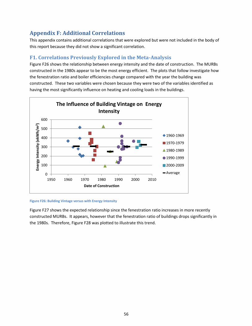
56
Appendix F: Additional Correlations This appendix contains additional correlations that were explored but were not included in the body of
this report because they did not show a significant correlation.
F1. Correlations Previously Explored in the Meta-Analysis Figure F26 shows the relationship between energy intensity and the date of construction. The MURBs
constructed in the 1980s appear to be the most energy efficient. The plots that follow investigate how
the fenestration ratio and boiler efficiencies change compared with the year the building was
constructed. These two variables were chosen because they were two of the variables identified as
having the most significantly influence on heating and cooling loads in the buildings.
Figure F26: Building Vintage versus with Energy Intensity
Figure F27 shows the expected relationship since the fenestration ratio increases in more recently
constructed MURBs. It appears, however that the fenestration ratio of buildings drops significantly in
the 1980s. Therefore, Figure F28 was plotted to illustrate this trend.
0
100
200
300
400
500
600
1950 1960 1970 1980 1990 2000 2010
Ene
rgy
Inte
nsi
ty (
ekW
h/m
2)
Date of Construction
The Influence of Building Vintage on Energy Intensity
1960-1969
1970-1979
1980-1989
1990-1999
2000-2009
Average
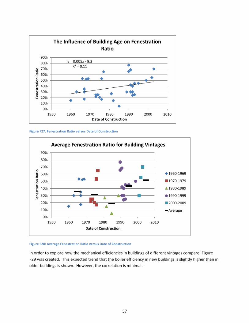
57
Figure F27: Fenestration Ratio versus Date of Construction
Figure F28: Average Fenestration Ratio versus Date of Construction
In order to explore how the mechanical efficiencies in buildings of different vintages compare, Figure
F29 was created. This expected trend that the boiler efficiency in new buildings is slightly higher than in
older buildings is shown. However, the correlation is minimal.
y = 0.005x - 9.3 R² = 0.11
0%
10%
20%
30%
40%
50%
60%
70%
80%
90%
1950 1960 1970 1980 1990 2000 2010
Fen
est
rati
on
Rat
io
Date of Construction
The Influence of Building Age on Fenestration Ratio
0%
10%
20%
30%
40%
50%
60%
70%
80%
90%
1950 1960 1970 1980 1990 2000 2010
Fen
est
rati
on
Rat
io
Date of Construction
Average Fenestration Ratio for Building Vintages
1960-1969
1970-1979
1980-1989
1990-1999
2000-2009
Average
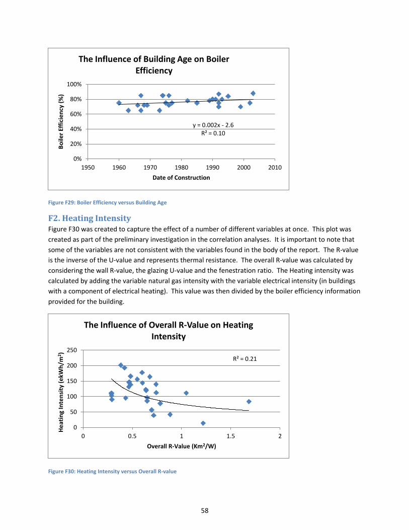
58
Figure F29: Boiler Efficiency versus Building Age
F2. Heating Intensity Figure F30 was created to capture the effect of a number of different variables at once. This plot was
created as part of the preliminary investigation in the correlation analyses. It is important to note that
some of the variables are not consistent with the variables found in the body of the report. The R-value
is the inverse of the U-value and represents thermal resistance. The overall R-value was calculated by
considering the wall R-value, the glazing U-value and the fenestration ratio. The Heating intensity was
calculated by adding the variable natural gas intensity with the variable electrical intensity (in buildings
with a component of electrical heating). This value was then divided by the boiler efficiency information
provided for the building.
Figure F30: Heating Intensity versus Overall R-value
y = 0.002x - 2.6 R² = 0.10
0%
20%
40%
60%
80%
100%
1950 1960 1970 1980 1990 2000 2010
Bo
iler
Effi
cie
ncy
(%
)
Date of Construction
The Influence of Building Age on Boiler Efficiency
R² = 0.21
0
50
100
150
200
250
0 0.5 1 1.5 2
He
atin
g In
ten
sity
(e
kWh
/m2 )
Overall R-Value (Km2/W)
The Influence of Overall R-Value on Heating Intensity
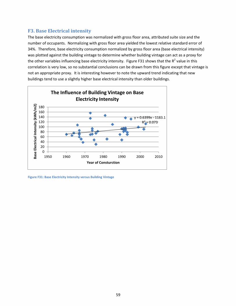
59
F3. Base Electrical intensity The base electricity consumption was normalized with gross floor area, attributed suite size and the
number of occupants. Normalizing with gross floor area yielded the lowest relative standard error of
34%. Therefore, base electricity consumption normalized by gross floor area (base electrical intensity)
was plotted against the building vintage to determine whether building vintage can act as a proxy for
the other variables influencing base electricity intensity. Figure F31 shows that the R2 value in this
correlation is very low, so no substantial conclusions can be drawn from this figure except that vintage is
not an appropriate proxy. It is interesting however to note the upward trend indicating that new
buildings tend to use a slightly higher base electrical intensity than older buildings.
Figure F31: Base Electricity Intensity versus Building Vintage
y = 0.6399x - 1183.1 R² = 0.073
0
20
40
60
80
100
120
140
160
180
1950 1960 1970 1980 1990 2000 2010 Bas
e E
lect
rica
l In
ten
sity
(kW
h/m
2)
Year of Consturction
The Influence of Building Vintage on Base Electricity Intensity
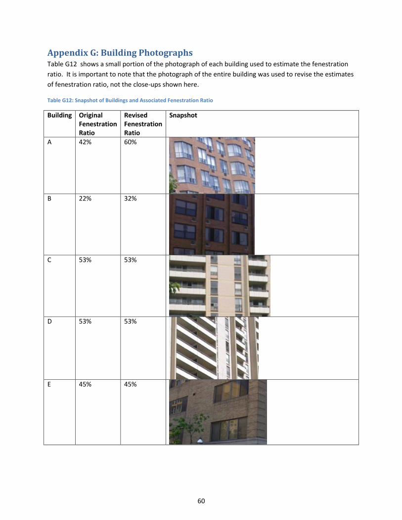
60
Appendix G: Building Photographs Table G12 shows a small portion of the photograph of each building used to estimate the fenestration
ratio. It is important to note that the photograph of the entire building was used to revise the estimates
of fenestration ratio, not the close-ups shown here.
Table G12: Snapshot of Buildings and Associated Fenestration Ratio
Building Original Fenestration Ratio
Revised Fenestration Ratio
Snapshot
A 42% 60%
B 22% 32%
C 53% 53%
D 53% 53%
E 45% 45%
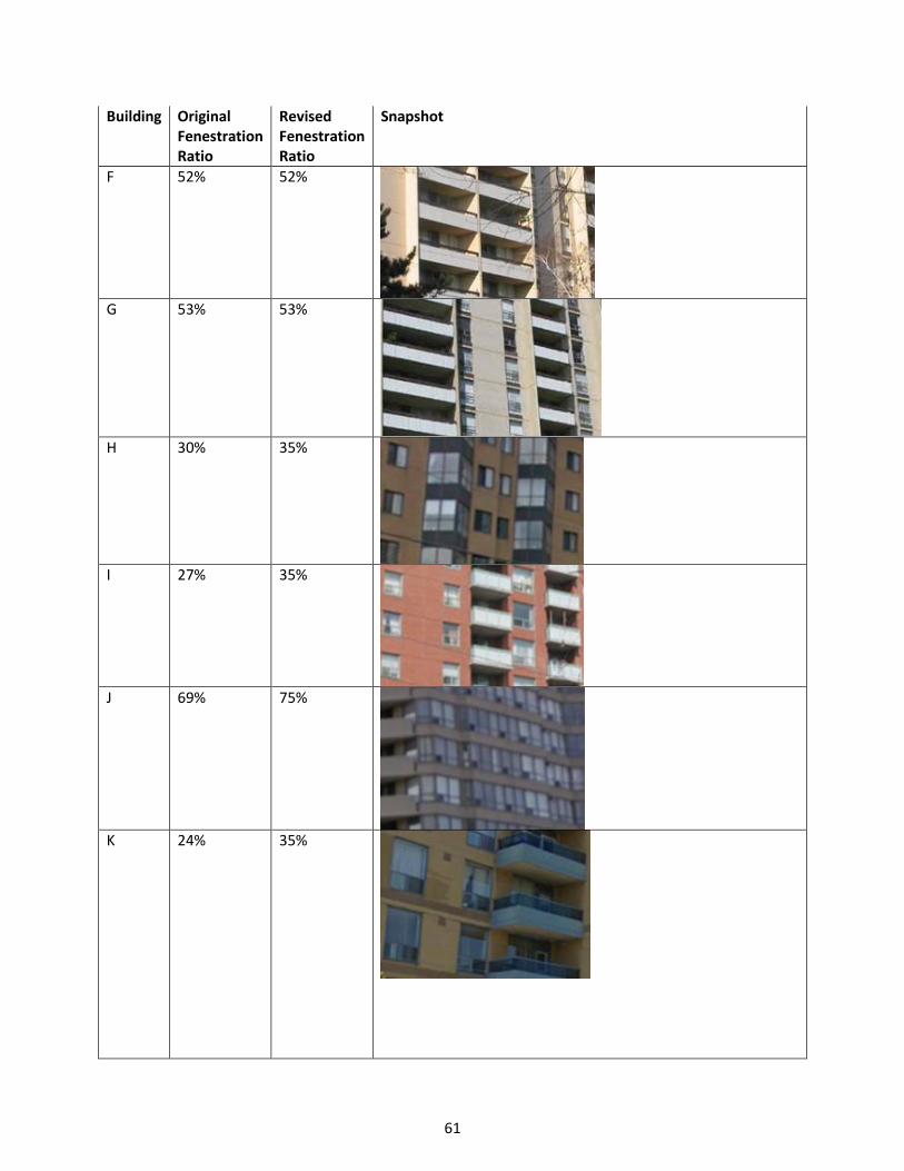
61
Building Original Fenestration Ratio
Revised Fenestration Ratio
Snapshot
F 52% 52%
G 53% 53%
H 30% 35%
I 27% 35%
J 69% 75%
K 24% 35%
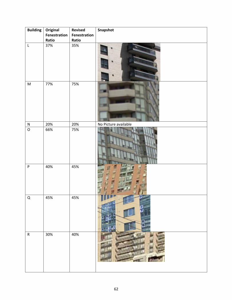
62
Building Original Fenestration Ratio
Revised Fenestration Ratio
Snapshot
L 37% 35%
M 77% 75%
N 20% 20% No Picture available
O 66% 75%
P 40% 45%
Q 45% 45%
R 30% 40%
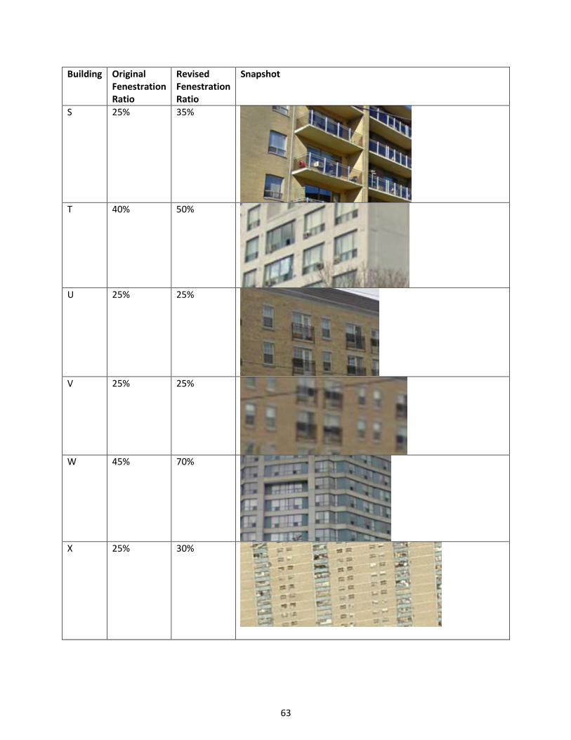
63
Building Original Fenestration Ratio
Revised Fenestration Ratio
Snapshot
S 25% 35%
T 40% 50%
U 25% 25%
V 25% 25%
W 45% 70%
X 25% 30%
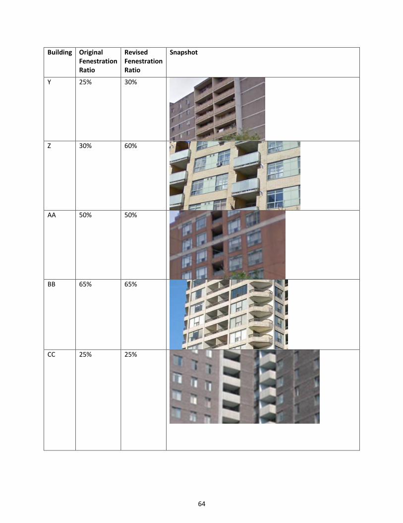
64
Building Original Fenestration Ratio
Revised Fenestration Ratio
Snapshot
Y 25% 30%
Z 30% 60%
AA 50% 50%
BB 65% 65%
CC 25% 25%
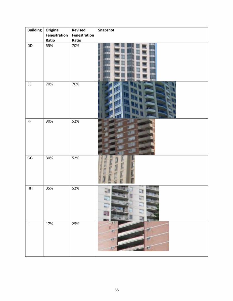
65
Building Original Fenestration Ratio
Revised Fenestration Ratio
Snapshot
DD 55% 70%
EE 70% 70%
FF 30% 52%
GG 30% 52%
HH 35% 52%
II 17% 25%
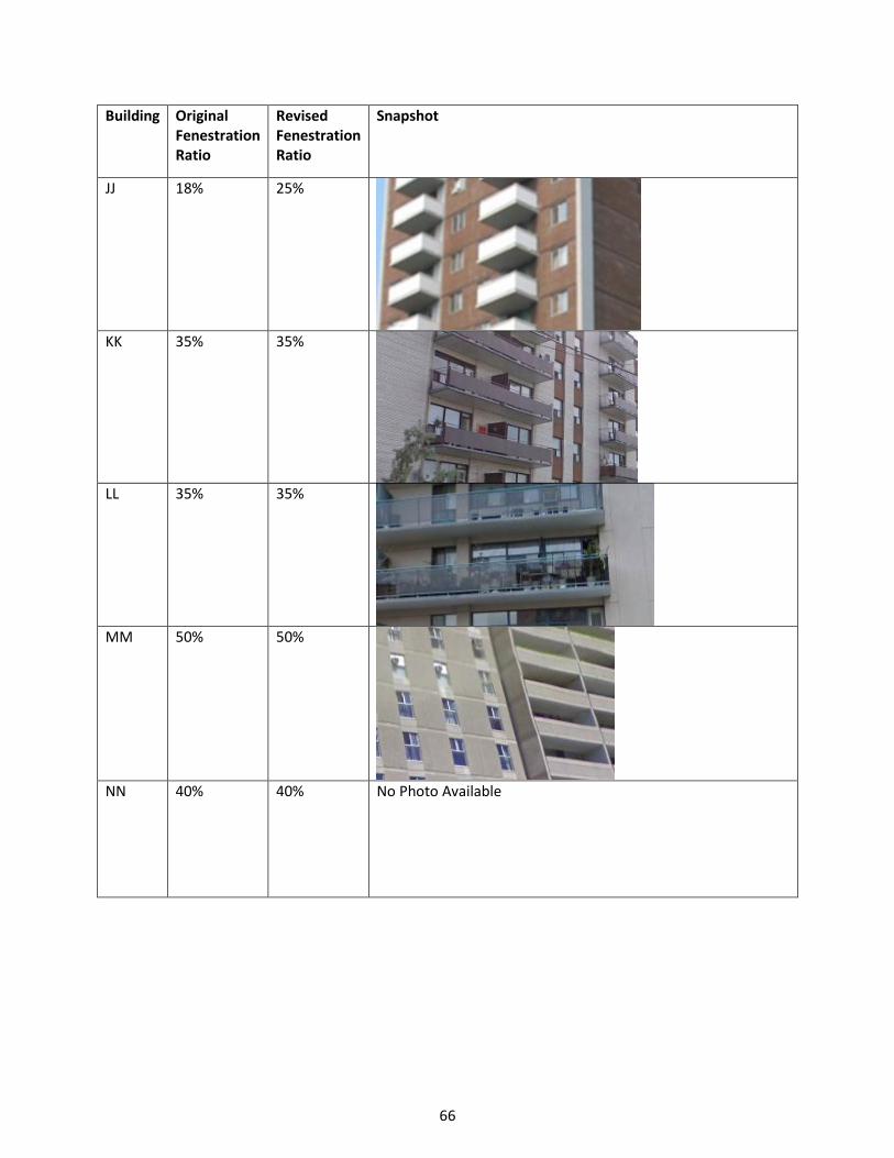
66
Building Original Fenestration Ratio
Revised Fenestration Ratio
Snapshot
JJ 18% 25%
KK 35% 35%
LL 35% 35%
MM 50% 50%
NN 40% 40% No Photo Available
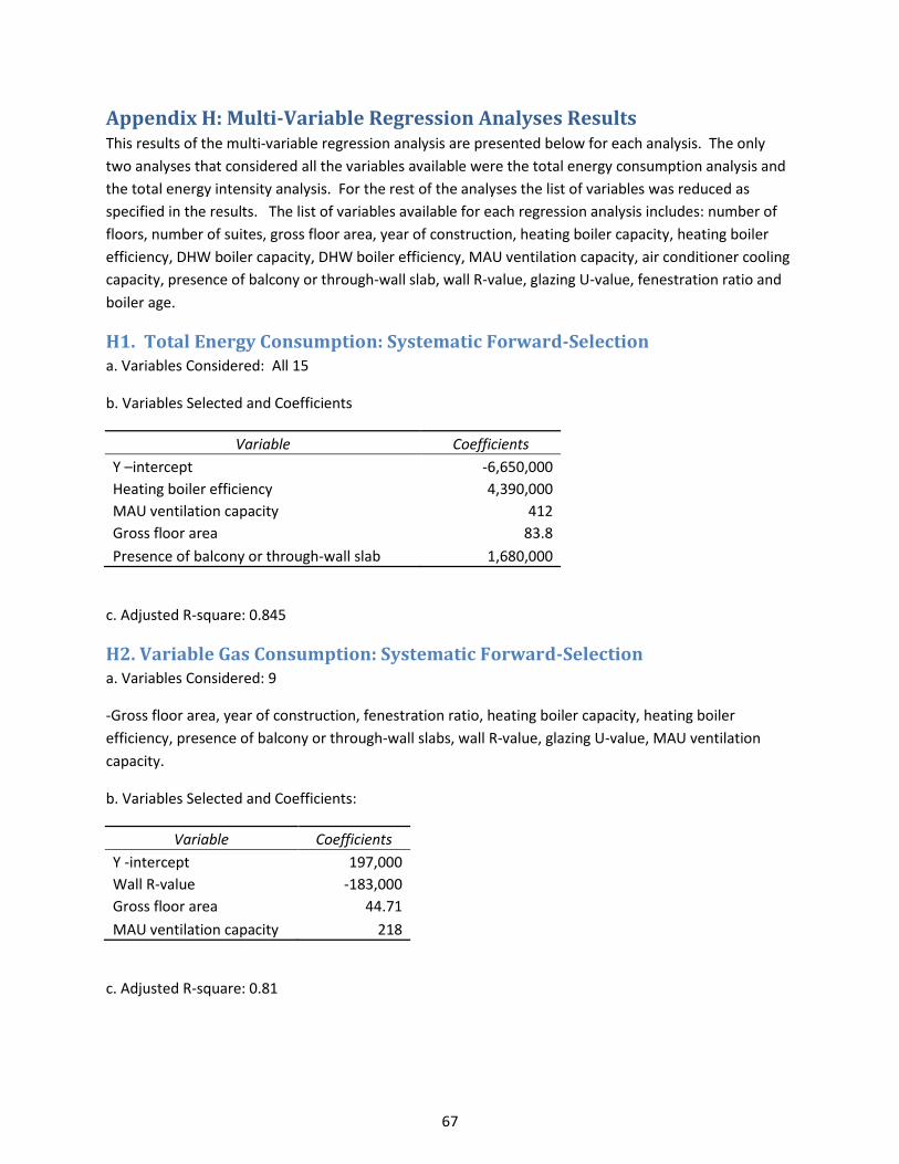
67
Appendix H: Multi-Variable Regression Analyses Results This results of the multi-variable regression analysis are presented below for each analysis. The only
two analyses that considered all the variables available were the total energy consumption analysis and
the total energy intensity analysis. For the rest of the analyses the list of variables was reduced as
specified in the results. The list of variables available for each regression analysis includes: number of
floors, number of suites, gross floor area, year of construction, heating boiler capacity, heating boiler
efficiency, DHW boiler capacity, DHW boiler efficiency, MAU ventilation capacity, air conditioner cooling
capacity, presence of balcony or through-wall slab, wall R-value, glazing U-value, fenestration ratio and
boiler age.
H1. Total Energy Consumption: Systematic Forward-Selection a. Variables Considered: All 15
b. Variables Selected and Coefficients
Variable Coefficients
Y –intercept -6,650,000
Heating boiler efficiency 4,390,000
MAU ventilation capacity 412
Gross floor area 83.8
Presence of balcony or through-wall slab 1,680,000
c. Adjusted R-square: 0.845
H2. Variable Gas Consumption: Systematic Forward-Selection a. Variables Considered: 9
-Gross floor area, year of construction, fenestration ratio, heating boiler capacity, heating boiler
efficiency, presence of balcony or through-wall slabs, wall R-value, glazing U-value, MAU ventilation
capacity.
b. Variables Selected and Coefficients:
Variable Coefficients
Y -intercept 197,000
Wall R-value -183,000
Gross floor area 44.71
MAU ventilation capacity 218
c. Adjusted R-square: 0.81
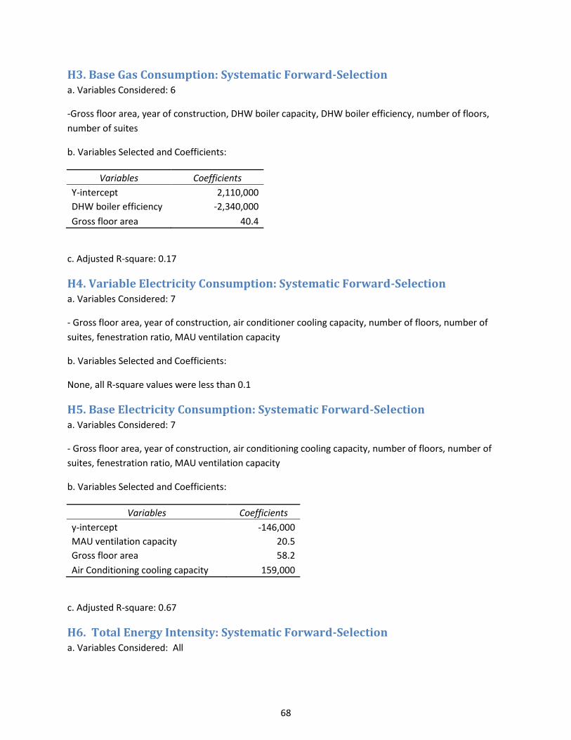
68
H3. Base Gas Consumption: Systematic Forward-Selection a. Variables Considered: 6
-Gross floor area, year of construction, DHW boiler capacity, DHW boiler efficiency, number of floors,
number of suites
b. Variables Selected and Coefficients:
Variables Coefficients
Y-intercept 2,110,000
DHW boiler efficiency -2,340,000
Gross floor area 40.4
c. Adjusted R-square: 0.17
H4. Variable Electricity Consumption: Systematic Forward-Selection a. Variables Considered: 7
- Gross floor area, year of construction, air conditioner cooling capacity, number of floors, number of
suites, fenestration ratio, MAU ventilation capacity
b. Variables Selected and Coefficients:
None, all R-square values were less than 0.1
H5. Base Electricity Consumption: Systematic Forward-Selection a. Variables Considered: 7
- Gross floor area, year of construction, air conditioning cooling capacity, number of floors, number of
suites, fenestration ratio, MAU ventilation capacity
b. Variables Selected and Coefficients:
Variables Coefficients
y-intercept -146,000
MAU ventilation capacity 20.5
Gross floor area 58.2
Air Conditioning cooling capacity 159,000
c. Adjusted R-square: 0.67
H6. Total Energy Intensity: Systematic Forward-Selection a. Variables Considered: All
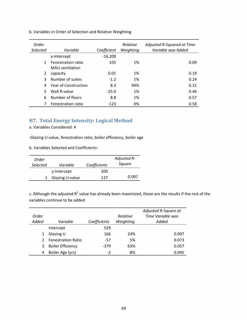
69
b. Variables in Order of Selection and Relative Weighting
Order Selected Variable Coefficient
Relative Weighting
Adjusted R-Squared at Time Variable was Added
y-Intercept -16,200
1 Fenestration ratio 335 1% 0.09
2 MAU ventilation capacity 0.01 1% 0.19
3 Number of suites -1.2 1% 0.24
4 Year of Construction 8.3 94% 0.31
5 Wall R-value -25.0 1% 0.46
6 Number of floors 8.8 1% 0.57
7 Fenestration ratio -123 0% 0.58
H7. Total Energy Intensity: Logical Method a. Variables Considered: 4
-Glazing U-value, fenestration ratio, boiler efficiency, boiler age
b. Variables Selected and Coefficients:
Order Selected Variable Coefficients
Adjusted R-Square
y-Intercept 200
1 Glazing U-value 137 0.097
c. Although the adjusted R2 value has already been maximized, these are the results if the rest of the
variables continue to be added
Order Added Variable Coefficients
Relative Weighting
Adjusted R-Square at Time Variable was
Added
Intercept 529
1 Glazing U 166 24% 0.097
2 Fenestration Ratio -57 5% 0.073
3 Boiler Efficiency -379 63% 0.057
4 Boiler Age (yrs) -2 8% 0.045