energy and water supply systems in remote regions ... · considering renewable energies and...
TRANSCRIPT
Energy and water supply systems in remote regionsconsidering renewable energies and seawater
desalination
Dipl.-Ing. Kristina Bognar
von der Fakultät III - Prozesswissenschaftender Technischen Universität Berlin
zur Erlangung des akademischen Grades
Doktorin der Ingenieurwissenschaften- Dr.-Ing. -
genehmigte Dissertation
Promotionsausschuss:Vorsitzender: Prof. Dr.-Ing. Felix ZieglerBerichter: Prof. Dr. Frank BehrendtBerichter: Prof. Dr. Ottmar Edenhofer
Tag der wissenschaftlichen Aussprache: 22. März 2013
Berlin, 2013D 83

3
Abstract
Islands and remote regions often depend on the import of fossil fuels for powergeneration. Due to the combined effect of high oil prices and transportation costs,energy supply systems based on renewable energies are already able to compete withfossil-fuel based supply systems successfully. A limiting factor for development inarid regions is the fresh water scarcity resulting from low natural water stocks andexcessive groundwater usage.
How seawater desalination and remote island-grids with a high share of renewableenergies can benefit each other, is still not sufficiently investigated. To answer thisand related research questions, a model for optimizing self-sufficient energy and watersupply systems has been developed, using the modeling language GAMS. Based onsets of hourly data various scenarios implementing energy conversion technologies,energy storage systems and desalination processes have been simulated and techno-economic optimizations accomplished. A global sensitivity and real option analysisaddresses optimal system designs and finance strategies taking uncertain demandand price developments into consideration.
Key findings reflect that the integration of renewable energies is beneficial. On theCape Verde island Brava, that has been chosen as a case study in the framework ofthis research, power is currently provided by diesel generators at prices of 0.25 to0.31e/kWh and water is sold for 2.35 and 4.93e/m3 depending on the quantity.With the recommended wind-battery-diesel and desalination supply system specificelectricity costs ranging from 0.15 to 0.21 e/kWh and water costs of 1.53e/m3 areachievable.
Effects of integrating desalination as a dynamic load complementing consumer in-duced load curves in stochastically fluctuating energy systems are analyzed as wellas the respective benefits highlighted: Excess wind energy, fuel consumption, andrequired energy storage capacities can be minimized resulting in lower specific elec-tricity costs. From five thermally and electrically driven desalination processes avariable operating reverse osmosis unit is the most flexible process facing intermit-tent and part-load operation.
To determine the technological and economic robustness of such an energy and wa-ter supply system the most sensitive parameters are identified and various analysesperformed. The approaches that have been introduced and respectively the resultsderived for the Cape Verde island Brava have been further underlined by investigat-ing comparable island-grids and are transferable to a global perspective.

5
Zusammenfassung
Inseln und abgelegene Regionen sind für die Energieversorgung häufig auf den Importfossiler Energieträger angewiesen. Auf Grund hoher Diesel- und Transportkostenrechnen sich Versorgungssysteme basierend auf erneuerbaren Energien wirtschaftlichschon heute. Ein limitierender Faktor für die Entwicklung arider Regionen ist dieWasserknappheit, die in der Regel auf geringe natürliche Wasservorkommen und dieÜbernutzung des Grundwassers zurückzuführen ist.
In wie weit Meerwasserentsalzungsanlagen in Inselnetzen mit einem hohen Anteilerneuerbarer Energien energetische und ökonomische Vorteile bringen kann, ist nochungenügend untersucht. Um diese und ähnliche Forschungsfragen beantworten zukönnen, wurde ein Modell zur Optimierung von autarken Energie- und Wasserver-sorgungskonzepten in der Modellierungsumgebung GAMS entwickelt. Basierend aufstündlich aufgelösten Nachfrage-, Windgeschwindigkeits- und Solareinstrahlungs-daten werden Szenarien techno-ökonomisch und ökologisch optimiert, in denen ver-schiedene Umwandlungstechniken regenerativer und fossiler Energien, thermischesowie elektrische Energiespeicher und Entsalzungsprozesse miteinander kombiniertwerden. Eine globale Sensitivitäts- und auch Realoptions-Analyse beschäftigt sichmit Effekten von Nachfrageveränderungen, preislichen sowie technologischen Un-sicherheiten und Ihren Auswirkungen auf ein langfristig robustes Versorgungskonzept.
Es wird gezeigt, dass die Integration von erneuerbaren Energien und der Meerwasser-entsalzung in allen untersuchten Inselnetzen vorteilhaft sein kann. Gegenstand derUntersuchung ist die kapverdische Insel Brava, wo der von Dieselmotoren gener-ierte Strom derzeit 0,25 bis 0,31e/kWh kostet und Trinkwasserpreise bei 2,35 bis4,93 e/m3 liegen. Unabhänging von der Preispolitik können mit dem errechnetenKonzept spezifische Stromkosten von 0,15 bis 0,21 e/kWh und Wasserkosten von1,53 e/m3 erreicht werden.
Weitere Ergebnisse sind u.a., dass eine Meerwasserentsalzungsanlage bei stark fluk-tuierenden Versorgungsstrukturen als dynamische Last Vorteile bringen kann: Über-schüssige Windenergie, der Dieselverbrauch sowie die Kapazität von Stromspeichernkönnen gesenkt werden und damit auch die spezifischen Stromkosten. Von den fünfbetrachteten Entsalzungstechnologien ist trotz der sensiblen Membrane die vari-abel betriebene Umkehrosmose-Anlage die robusteste im Umgang mit unstetiger,anteiliger und abreißender Energieversorgung.
Um die technologische und ökonomische Verlässlichkeit und Optimalität des Ver-sorgungskonzepts prüfen zu können, werden die sensibelsten Parameter bestimmtund deren Auswirkungen in weitreichenden Sensitivitätsanalysen untersucht. Vor-gestellte Ansätze und Ergebnisse können durch die Betrachtung von ähnlichen In-selnetzen bestätigt und daher auch global auf weitere Regionen übertragen werden.

Contents
1 Introduction 1
1.1 Motivation . . . . . . . . . . . . . . . . . . . . . . . . . . . . . . . . . 1
1.2 Research objective . . . . . . . . . . . . . . . . . . . . . . . . . . . . 3
1.3 Structure of thesis . . . . . . . . . . . . . . . . . . . . . . . . . . . . 4
2 Background 5
2.1 Energy supply structures . . . . . . . . . . . . . . . . . . . . . . . . . 5
2.1.1 Demand Side Management . . . . . . . . . . . . . . . . . . . . 6
2.1.2 Renewable power generation in island grids . . . . . . . . . . . 7
2.2 Renewable energy technologies . . . . . . . . . . . . . . . . . . . . . . 9
2.2.1 Photovoltaics . . . . . . . . . . . . . . . . . . . . . . . . . . . 9
2.2.2 Concentrated Solar Power . . . . . . . . . . . . . . . . . . . . 10
2.2.3 Wind energy converters . . . . . . . . . . . . . . . . . . . . . 13
2.3 Energy storage systems . . . . . . . . . . . . . . . . . . . . . . . . . . 14
2.3.1 Thermal energy storage systems . . . . . . . . . . . . . . . . . 14
2.3.2 Electricity storage systems . . . . . . . . . . . . . . . . . . . . 16
2.4 Backup system . . . . . . . . . . . . . . . . . . . . . . . . . . . . . . 21
2.5 Seawater desalination in remote regions . . . . . . . . . . . . . . . . . 22
2.5.1 Basics of water . . . . . . . . . . . . . . . . . . . . . . . . . . 22
2.5.2 Desalination processes . . . . . . . . . . . . . . . . . . . . . . 24
2.5.3 Variable operating desalination . . . . . . . . . . . . . . . . . 30
2.5.4 Desalination powered by renewable energies . . . . . . . . . . 31
2.6 Small Island Developing States . . . . . . . . . . . . . . . . . . . . . 33
II Contents
3 Methodology 36
3.1 Simulation of energy systems . . . . . . . . . . . . . . . . . . . . . . . 36
3.2 Simulation of desalination units . . . . . . . . . . . . . . . . . . . . . 39
3.3 Optimization approach . . . . . . . . . . . . . . . . . . . . . . . . . . 41
3.3.1 GAMS/OSICplex . . . . . . . . . . . . . . . . . . . . . . . . . 42
3.3.2 Characteristics of developed program . . . . . . . . . . . . . . 43
3.4 Sensitivity analysis . . . . . . . . . . . . . . . . . . . . . . . . . . . . 47
3.5 Real option analysis . . . . . . . . . . . . . . . . . . . . . . . . . . . 48
3.6 Ecological constraints within the model . . . . . . . . . . . . . . . . . 51
4 Model 53
4.1 Objective function and main constraints . . . . . . . . . . . . . . . . 54
4.2 Modeling total costs . . . . . . . . . . . . . . . . . . . . . . . . . . . 57
4.3 Modeling photovoltaic energy generation systems . . . . . . . . . . . 58
4.3.1 Modeling energy flows (PV) . . . . . . . . . . . . . . . . . . . 58
4.3.2 Modeling total costs (PV) . . . . . . . . . . . . . . . . . . . . 58
4.4 Modeling concentrated solar power systems . . . . . . . . . . . . . . . 59
4.4.1 Modeling energy flows (CSP) . . . . . . . . . . . . . . . . . . 59
4.4.2 Modeling total costs (CSP) . . . . . . . . . . . . . . . . . . . 60
4.5 Modeling wind energy generation systems . . . . . . . . . . . . . . . 60
4.5.1 Modeling energy flows (wind) . . . . . . . . . . . . . . . . . . 60
4.5.2 Modeling total costs (wind) . . . . . . . . . . . . . . . . . . . 62
4.6 Modeling diesel generator systems . . . . . . . . . . . . . . . . . . . . 62
4.6.1 Modeling energy flows (diesel) . . . . . . . . . . . . . . . . . . 62
4.6.2 Modeling total costs (diesel) . . . . . . . . . . . . . . . . . . . 65
4.7 Modeling desalination systems . . . . . . . . . . . . . . . . . . . . . . 66
4.7.1 Modeling energy flows (Desal) . . . . . . . . . . . . . . . . . . 66
4.7.2 Modeling total costs (Desal) . . . . . . . . . . . . . . . . . . . 67
4.8 Modeling energy and water storages . . . . . . . . . . . . . . . . . . . 67
4.8.1 Modeling electricity storage systems (ESS) . . . . . . . . . . . 68
4.8.2 Modeling thermal energy storage systems (TSS) . . . . . . . . 71
4.8.3 Modeling water storage systems (WSS) . . . . . . . . . . . . . 72
Contents III
4.9 Limitations of the model . . . . . . . . . . . . . . . . . . . . . . . . . 72
4.9.1 Time discretization . . . . . . . . . . . . . . . . . . . . . . . . 73
4.9.2 Boundaries and mutual exclusivity . . . . . . . . . . . . . . . 73
4.9.3 Reduction of computational cost . . . . . . . . . . . . . . . . . 74
4.9.4 Capacity of diesel generators . . . . . . . . . . . . . . . . . . . 76
5 Case Study: A Cape Verde island 78
5.1 Background of Cape Verde . . . . . . . . . . . . . . . . . . . . . . . . 78
5.2 Energy and water demand on Brava . . . . . . . . . . . . . . . . . . . 80
5.3 Renewable energy potential . . . . . . . . . . . . . . . . . . . . . . . 81
5.4 Input data in the model . . . . . . . . . . . . . . . . . . . . . . . . . 84
5.4.1 Economic input data . . . . . . . . . . . . . . . . . . . . . . . 84
5.4.2 Input data PV-systems . . . . . . . . . . . . . . . . . . . . . . 84
5.4.3 Input data CSP . . . . . . . . . . . . . . . . . . . . . . . . . . 85
5.4.4 Input data wind energy converters . . . . . . . . . . . . . . . 86
5.4.5 Input data diesel generators . . . . . . . . . . . . . . . . . . . 87
5.4.6 Input data Electricity Storage Systems . . . . . . . . . . . . . 88
5.4.7 Input data thermal energy storage systems . . . . . . . . . . . 89
5.4.8 Input data Desalination . . . . . . . . . . . . . . . . . . . . . 90
5.4.9 Input data water storage system . . . . . . . . . . . . . . . . . 91
6 Results 92
6.1 Validation of model . . . . . . . . . . . . . . . . . . . . . . . . . . . . 92
6.2 The optimal energy and water supply system . . . . . . . . . . . . . . 95
6.3 Supply scenarios in comparison . . . . . . . . . . . . . . . . . . . . . 96
6.3.1 Integrating renewable energies into the current supply system 96
6.3.2 The optimal desalination process . . . . . . . . . . . . . . . . 99
6.3.3 Robustness of the optimal desalination system . . . . . . . . . 104
6.3.4 Optimal electricity storage system . . . . . . . . . . . . . . . . 105
6.4 Interference of energy storage systems and desalination processes . . . 107
6.5 Approach and results of a global sensitivity analysis . . . . . . . . . . 110
6.5.1 Impact of wind velocity and solar irradiation . . . . . . . . . . 110
6.5.2 Definition of parameters . . . . . . . . . . . . . . . . . . . . . 111
IV Contents
6.5.3 Sensitivity of parameters . . . . . . . . . . . . . . . . . . . . . 113
6.5.4 Probability of technology implementations . . . . . . . . . . . 116
6.5.5 Impact of sensitive parameters on the energy supply system . 119
6.5.6 Impact of sensitive parameters on the desalination unit . . . . 123
6.6 Economic reflection: Investment strategies based on the real optionapproach (ROA) . . . . . . . . . . . . . . . . . . . . . . . . . . . . . 127
6.7 Global reflection: Concepts for other islands . . . . . . . . . . . . . . 131
7 Conclusions 134
7.1 Summary and conclusions . . . . . . . . . . . . . . . . . . . . . . . . 134
7.2 Recommendations for further research . . . . . . . . . . . . . . . . . 138
Bibliography 143
A Model Script 154
B Renewable energy technologies not modeled 185
B.1 Hydro power . . . . . . . . . . . . . . . . . . . . . . . . . . . . . . . . 185
B.2 Ocean powers . . . . . . . . . . . . . . . . . . . . . . . . . . . . . . . 186
B.3 Geothermal energy . . . . . . . . . . . . . . . . . . . . . . . . . . . . 188
B.4 Energetic use of biomass . . . . . . . . . . . . . . . . . . . . . . . . . 189
C Renewable energy powered desalination 192
List of Figures
2.1 Simple chain from extraction to end-use within an energy supply system 5
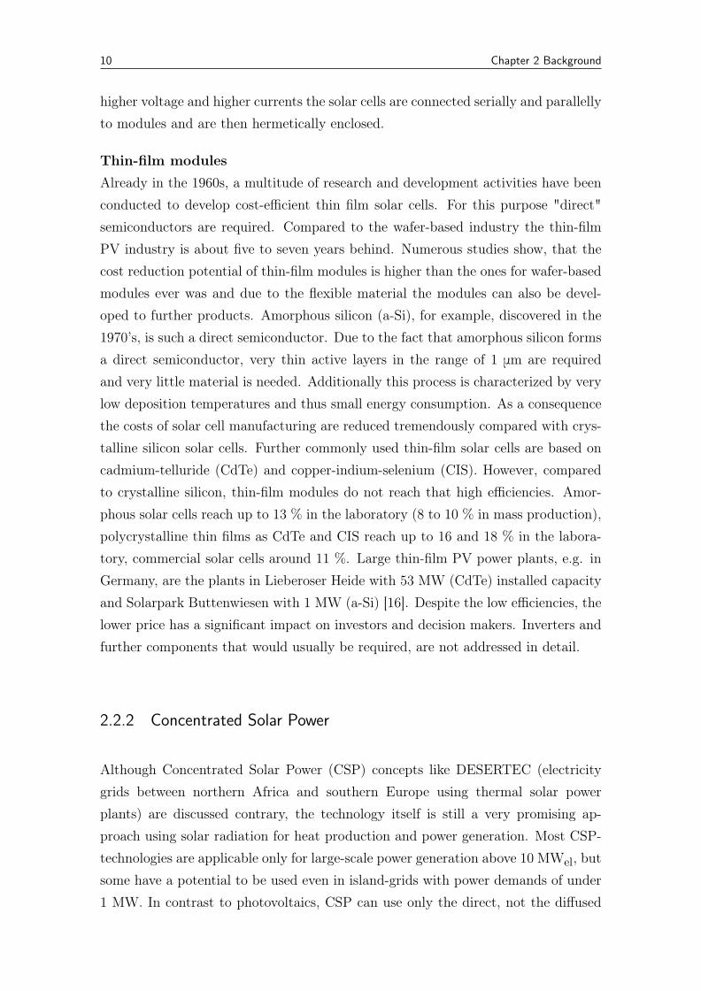
2.2 Parabolic Trough (upper left), Linear Fresnel (bottom left), Solartower (upper right) and Solar Dish (bottom right) [17] . . . . . . . . 11
2.3 Types of thermal energy storage systems . . . . . . . . . . . . . . . . 14
2.4 Ragone Diagram of electrochemical storages . . . . . . . . . . . . . . 19
2.5 Global stock of water [38] . . . . . . . . . . . . . . . . . . . . . . . . 23
2.6 Overview of desalination methods . . . . . . . . . . . . . . . . . . . . 24
2.7 Multi-effect distillation process [126] . . . . . . . . . . . . . . . . . . 25
2.8 Humidification-dehumidification process [126] . . . . . . . . . . . . . 27
2.9 Membrane distillation process [44] . . . . . . . . . . . . . . . . . . . . 28
2.10 Mechanical vapour compression process [127] . . . . . . . . . . . . . . 29
2.11 Reverse osmosis process [127] . . . . . . . . . . . . . . . . . . . . . . 29
2.12 Technology combinations RE-powered desalination plants . . . . . . . 31
2.13 Concept of Enercon wind-RO system [41] . . . . . . . . . . . . . . . . 33
2.14 Development stage and capacity range of the main RE-desalinationtechnologies [46] . . . . . . . . . . . . . . . . . . . . . . . . . . . . . . 34
2.15 SIDS worldwide . . . . . . . . . . . . . . . . . . . . . . . . . . . . . . 35
3.1 Modeling programs for energy systems in comparison . . . . . . . . . 37
3.2 Overview of the optimization approach . . . . . . . . . . . . . . . . . 41
3.3 Methodology overview . . . . . . . . . . . . . . . . . . . . . . . . . . 43
3.4 Flow chart of optimization approach . . . . . . . . . . . . . . . . . . 45
3.5 Trajectory example of Morris analysis (left) and relevance of param-eters (right) . . . . . . . . . . . . . . . . . . . . . . . . . . . . . . . . 47
3.6 Binomial pricing tree for two periods: Diesel price development in 20years . . . . . . . . . . . . . . . . . . . . . . . . . . . . . . . . . . . . 51
VI List of Figures
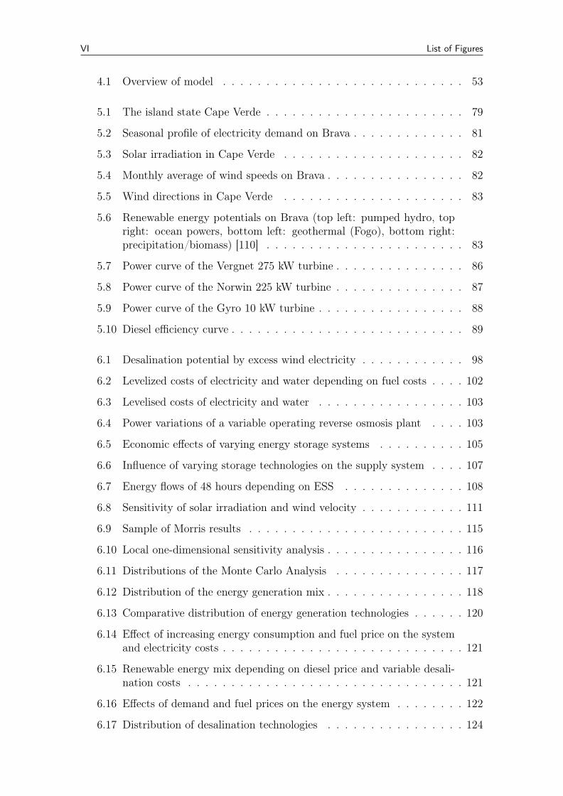
4.1 Overview of model . . . . . . . . . . . . . . . . . . . . . . . . . . . . 53
5.1 The island state Cape Verde . . . . . . . . . . . . . . . . . . . . . . . 79
5.2 Seasonal profile of electricity demand on Brava . . . . . . . . . . . . . 81
5.3 Solar irradiation in Cape Verde . . . . . . . . . . . . . . . . . . . . . 82
5.4 Monthly average of wind speeds on Brava . . . . . . . . . . . . . . . . 82
5.5 Wind directions in Cape Verde . . . . . . . . . . . . . . . . . . . . . 83
5.6 Renewable energy potentials on Brava (top left: pumped hydro, topright: ocean powers, bottom left: geothermal (Fogo), bottom right:precipitation/biomass) [110] . . . . . . . . . . . . . . . . . . . . . . . 83
5.7 Power curve of the Vergnet 275 kW turbine . . . . . . . . . . . . . . . 86
5.8 Power curve of the Norwin 225 kW turbine . . . . . . . . . . . . . . . 87
5.9 Power curve of the Gyro 10 kW turbine . . . . . . . . . . . . . . . . . 88
5.10 Diesel efficiency curve . . . . . . . . . . . . . . . . . . . . . . . . . . . 89
6.1 Desalination potential by excess wind electricity . . . . . . . . . . . . 98
6.2 Levelized costs of electricity and water depending on fuel costs . . . . 102
6.3 Levelised costs of electricity and water . . . . . . . . . . . . . . . . . 103
6.4 Power variations of a variable operating reverse osmosis plant . . . . 103
6.5 Economic effects of varying energy storage systems . . . . . . . . . . 105
6.6 Influence of varying storage technologies on the supply system . . . . 107
6.7 Energy flows of 48 hours depending on ESS . . . . . . . . . . . . . . 108
6.8 Sensitivity of solar irradiation and wind velocity . . . . . . . . . . . . 111
6.9 Sample of Morris results . . . . . . . . . . . . . . . . . . . . . . . . . 115
6.10 Local one-dimensional sensitivity analysis . . . . . . . . . . . . . . . . 116
6.11 Distributions of the Monte Carlo Analysis . . . . . . . . . . . . . . . 117
6.12 Distribution of the energy generation mix . . . . . . . . . . . . . . . . 118
6.13 Comparative distribution of energy generation technologies . . . . . . 120
6.14 Effect of increasing energy consumption and fuel price on the systemand electricity costs . . . . . . . . . . . . . . . . . . . . . . . . . . . . 121
6.15 Renewable energy mix depending on diesel price and variable desali-nation costs . . . . . . . . . . . . . . . . . . . . . . . . . . . . . . . . 121
6.16 Effects of demand and fuel prices on the energy system . . . . . . . . 122
6.17 Distribution of desalination technologies . . . . . . . . . . . . . . . . 124
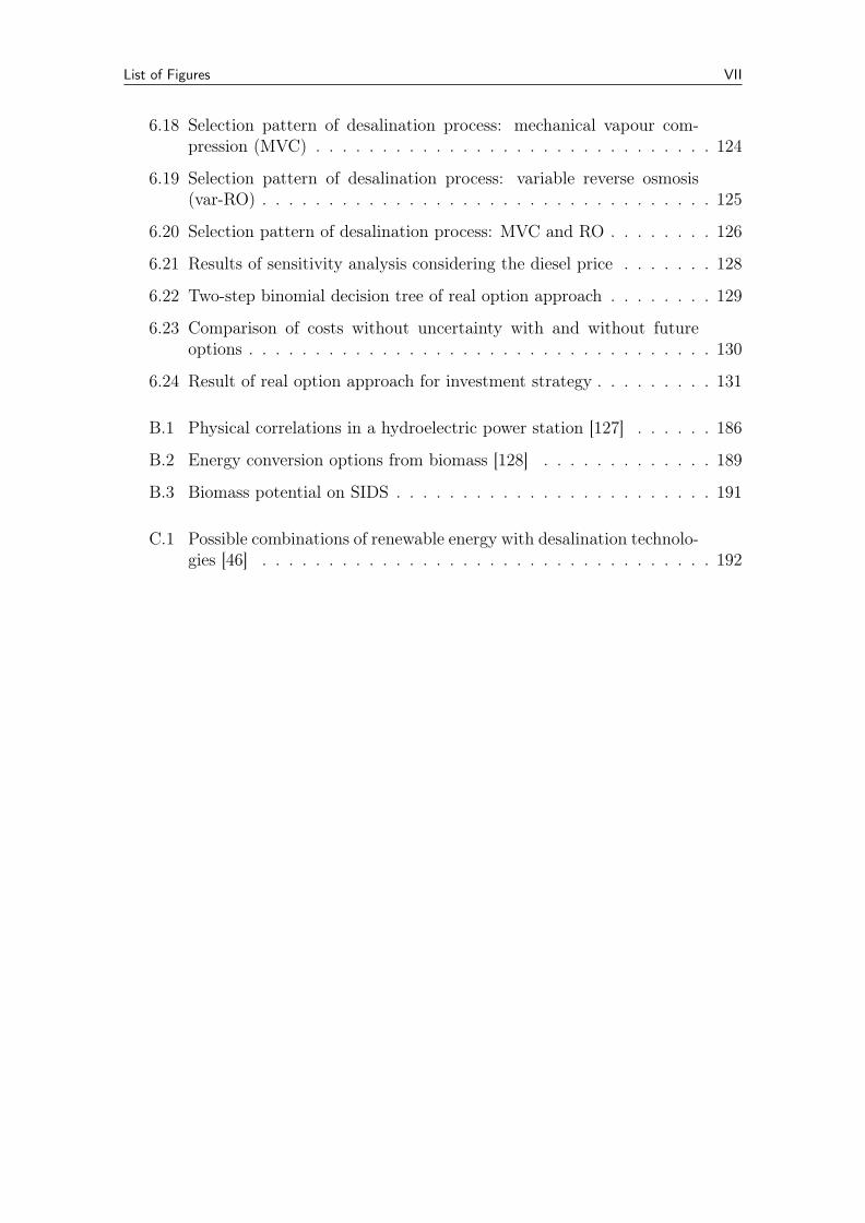
List of Figures VII
6.18 Selection pattern of desalination process: mechanical vapour com-pression (MVC) . . . . . . . . . . . . . . . . . . . . . . . . . . . . . . 124
6.19 Selection pattern of desalination process: variable reverse osmosis(var-RO) . . . . . . . . . . . . . . . . . . . . . . . . . . . . . . . . . . 125
6.20 Selection pattern of desalination process: MVC and RO . . . . . . . . 126
6.21 Results of sensitivity analysis considering the diesel price . . . . . . . 128
6.22 Two-step binomial decision tree of real option approach . . . . . . . . 129
6.23 Comparison of costs without uncertainty with and without futureoptions . . . . . . . . . . . . . . . . . . . . . . . . . . . . . . . . . . . 130
6.24 Result of real option approach for investment strategy . . . . . . . . . 131
B.1 Physical correlations in a hydroelectric power station [127] . . . . . . 186
B.2 Energy conversion options from biomass [128] . . . . . . . . . . . . . 189
B.3 Biomass potential on SIDS . . . . . . . . . . . . . . . . . . . . . . . . 191
C.1 Possible combinations of renewable energy with desalination technolo-gies [46] . . . . . . . . . . . . . . . . . . . . . . . . . . . . . . . . . . 192
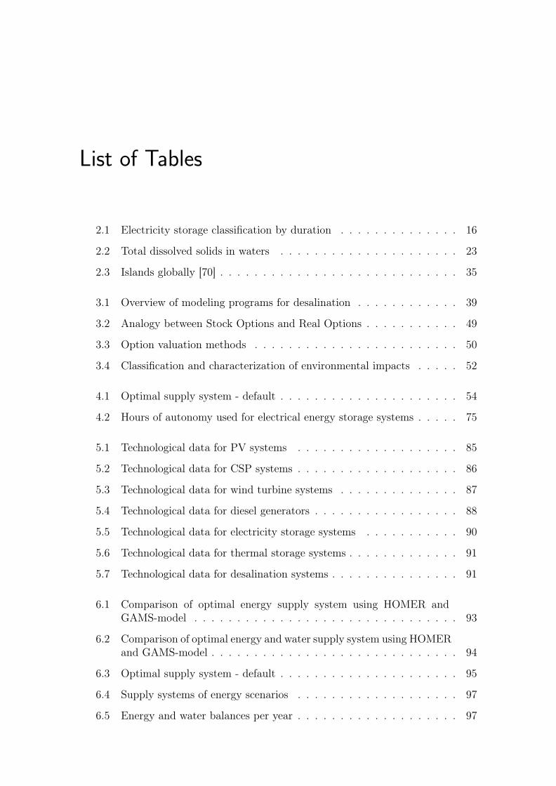
List of Tables
2.1 Electricity storage classification by duration . . . . . . . . . . . . . . 16
2.2 Total dissolved solids in waters . . . . . . . . . . . . . . . . . . . . . 23
2.3 Islands globally [70] . . . . . . . . . . . . . . . . . . . . . . . . . . . . 35
3.1 Overview of modeling programs for desalination . . . . . . . . . . . . 39
3.2 Analogy between Stock Options and Real Options . . . . . . . . . . . 49
3.3 Option valuation methods . . . . . . . . . . . . . . . . . . . . . . . . 50
3.4 Classification and characterization of environmental impacts . . . . . 52
4.1 Optimal supply system - default . . . . . . . . . . . . . . . . . . . . . 54
4.2 Hours of autonomy used for electrical energy storage systems . . . . . 75
5.1 Technological data for PV systems . . . . . . . . . . . . . . . . . . . 85
5.2 Technological data for CSP systems . . . . . . . . . . . . . . . . . . . 86
5.3 Technological data for wind turbine systems . . . . . . . . . . . . . . 87
5.4 Technological data for diesel generators . . . . . . . . . . . . . . . . . 88
5.5 Technological data for electricity storage systems . . . . . . . . . . . 90
5.6 Technological data for thermal storage systems . . . . . . . . . . . . . 91
5.7 Technological data for desalination systems . . . . . . . . . . . . . . . 91
6.1 Comparison of optimal energy supply system using HOMER andGAMS-model . . . . . . . . . . . . . . . . . . . . . . . . . . . . . . . 93
6.2 Comparison of optimal energy and water supply system using HOMERand GAMS-model . . . . . . . . . . . . . . . . . . . . . . . . . . . . . 94
6.3 Optimal supply system - default . . . . . . . . . . . . . . . . . . . . . 95
6.4 Supply systems of energy scenarios . . . . . . . . . . . . . . . . . . . 97
6.5 Energy and water balances per year . . . . . . . . . . . . . . . . . . . 97

List of Tables IX
6.6 Deviations within the local sensitivity analysis concerning desalination 104
6.7 Input parameters for sensitivity . . . . . . . . . . . . . . . . . . . . . 112
6.8 Output variables for sensitivity . . . . . . . . . . . . . . . . . . . . . 113
6.9 Numerical results of Morris approach . . . . . . . . . . . . . . . . . . 114
6.10 Supply system scenarios for the real option analysis . . . . . . . . . . 128
6.11 Properties of other considered islands . . . . . . . . . . . . . . . . . . 132
List of Acronyms
a-Si Amorphous silicon thin-film solar cellAOSIS Alliance of Small Island StatesBaU Business as usual (scenario)bin Binary variable to identify the interpolation range
for diesel efficiency linearisationcCO2 Specific carbon dioxide emission cost [e/tCO2]cE,O&M O&M cost as a specific cost based on the electricity
produced[e/kWh y]
cfuel Specific fuel oil cost based on the energy inside thefuel
[e/kWhfuel]
cland Specific mean land cost [e/m2]cP,O&M O&M cost as a specific cost based on the installed
power[e/kW y]
cplant Capacity specific cost of the type of desalinationplant
[e/(m3/d)]
crep,E Specific energy replacement cost [ e/kWhreplacement ]
crep,P Specific power replacement cost [ e/kWreplacement ]
cRes Specific cost of resource consumption and deple-tion
[e/t]
cw,O&M O&M cost as a specific cost based on the waterproduced
[e/kWh y]
cwss Specific capacity investment cost [e/m3]cE Specific energy investment cost [e/kWh]cP Specific power investment cost [e/kW]c-Si multi crystalline solar cellsCAES Compressed air energy storageCapacityDesal Installed production capacity of desalination plant
technology[m3/d]
CdTe cadmium-telluride thin-film photovoltaic moduleCIS copper-indium-selenium thin-film photovoltaic
moduleCSP Label of the concentrated solar power subsystemd Set of all days in the time-frame of the modelDSM Demand Side ManagementDerationi Losses coefficient of subsystem “i” other then con-
version[-]
List of Tables XI
Desal Label of the desalination subsystemdiesel Label of the diesel generators subsystemDP Diesel priceDumpel Flux of electric energy being dumped out of the
system[kWh/h]
Dumpth Flux of thermal energy being dumped out of thesystem
[kWh/h]
Econs,el Electricity consumption of the desalination systemto produce desalted water
[kWh/m3]
Ei,in Flux of electric energy entering the technology ofsubsystem “i”
[kWh/h]
Ei,out Flux of electric energy leaving the technology ofsubsystem “i”
[kWh/h]
Ei Installed energy capacity of the technology of sub-system “i”
[kWh/h]
ESS Label of the electric energy storage subsystemη Efficiency of conversion or round-trip efficiency [-]ηel Electrical efficiency of conversion, produced elec-
tricity - spent energy ratio[-]
ηth Thermal efficiency of conversion, produced ther-mal energy - spent energy ratio
[-]
Existi Binary variable that allow the size of the systemto be either inside the range or zero
fO&M O&M cost factor as a percentage of the investmentcost
[y–1]
FLH Full load hours [h/y]i Interest rate [–]H2PEMFC Hydrogen energy storage system with proton ex-
change membrane (fuel cell)H2Engine Hydrogen energy storage system coupled with
combustion engineHDH Humidification-Dehumidification (desalination
technology)kCO2 Energy specific CO2 emission from the fuel [ tCO2
kWhfuel]
kLU Area coefficient for auxiliary space needed [-]LA Lead-acid batteryλ Weighting factor of interpolation for diesel effi-
ciency linearisation[-]
LCoE Levelized costs of electricity [e/kWh]LCoW Levelized costs of water [e/m3]Li-ion Lithium-ion batteryLoad The hourly electric load of the island under exam [kWh/h]Losses The hourly parasitic losses in terms of fraction of
the energy stored[h–1]
LUi Specific land use of the technology of subsystem“i”
[m2/kW]
XII List of Tables
MaxPi Maximum size bound for the technology of subsys-tem “i”
[kW]
MD Membrane Distillation (desalination technology)MED Multi-Effect Distillation (desalination technology)MVC Mechanical Vapour Compression (desalination
technology)MinPi Minimum size bound for the technology of subsys-
tem “i”[kW]
NaS Sodium-sulphur batteryNiCd Nickel-cadmium batteryNPC Net present costsORC Organic rankine cyclep risk-neutral probabilityPi Installed rated (or peak) power of the technology
of subsystem “i”[kW]
PW,nom Rated power of the standard wind turbine [kW]PCM Phase change materialsPHS pumped hydroelectric energy storage systempts Set of all points used in diesel efficiency lineariza-
tionPV Photovoltaics and label of the photovoltaic subsys-
temr risk-free rate of returnRES Renewable energy sourcesRO Reverse osmosis (desalination technology)ROA Real option analysisSIDS Small Island Developing Statesσ2 standard deviation (in ROA)
SolarRadiation Specific incoming solar radiation based on meteo-rological data
[kW/m2]
SOS Special order sets (Modeling)SpecificOutput Specific electrical energy output of the standard
wind turbine[kWh/h]
Storedel Amount of electrical energy stored in ess’ (that canbe totally released)
[kWh]
Storedth Amount of thermal energy stored in tss’ (that canbe totally released)
[kWh]
t Set of all hours in the time-frame of the modelTCi Total cost of the technology of subsystem “i” [e]Thi,in Flux of thermal energy entering the technology of
subsystem “i”[kWh/h]
Thi,out Flux of thermal energy leaving the technology ofsubsystem “i”
[kWh/h]
TSS Label of the thermal energy storage subsystemVwss Installed storage capacity of the water storage [m3]Vcut–in wind velocities, here cut-in [m/s]V-redox Vanadium-redox-flow battery
List of Tables XIII
var-RO variable reverse osmosis (desalination technology)W Label of the wind turbine subsystemWaterreserve The amount of water stored in the water storage
system[m3]
WaterDemand The daily water demand of the island under exam [m3/d]WaterGenDesal hourly water output of the desalination system [m3/d]WEC Wind energy converterWind1 scenario with small wind capacityWind2 scenario with large wind capacityWind1+PV scenario with small wind capacity und PV systemsWSS Label of the water storage subsystemy yearZnBr zinc-bromine flow batteryξ Binary variable used to trigger the mutual exclu-
sivity of some model variables

XIV List of Tables
Chapter
1Introduction
1.1 Motivation
Globally, many developing regions face insufficient power supply and the lack of cleanfreshwater. Especially remote regions depend highly on stand-alone infrastructuresystems and therefore often on the import of fossil fuels. As a preliminary work forremote regions in general, the focus is set on islands, investigating the challengesand chances of island-grids approaching a high share of renewable energies. Dueto the combined effect of high transportation costs and increasing oil prices, whichoften range two or three times above onshore market price, energy supply systemsbased on renewable energies are already able to compete successfully with fossil-fuelbased supply systems.
In remote and arid regions, there is not only a need to guarantee power generation,but also supplying freshwater is a common challenge. Global desertification andexcessive usage of natural freshwater reservoirs diminish accessible water stocks. Onislands, the unlimited usage of groundwater results in an inflow of seawater fromnearby coastlines, leading to increased salt levels and making the previous freshwa-ter unfit for human consumption and other applications. Many islands, therefore,depend also highly on freshwater imports. Ecologically friendly seawater desalina-tion could provide a promising alternative that offers a reliable and, in many cases,less expensive water supply than the import by ships [1]. Combining renewable en-ergy grids and desalination can have promising advantages: It needs to be provenwhether implementing desalination as deferrable load, as a shiftable energy sink,can minimize unused dump-load, minimize the demand of electricity storage sys-tems and minimize energy costs for desalination. Generally, the main question tobe answered in this work is, how seawater desalination and island-grids with
2 Chapter 1 Introduction
a high share of renewable energies can benefit each other. Related researchapproaches deal mainly either with large-scale or small-scale applications. Theyusually try to answer following questions:
• how frequency stabilization can be reached in large grids, e.g in the UCTE inEurope, by energy storage systems or demand side management,• how energy can be provided efficiently and/or renewable for large desalination
plants of 500,000-1,000,000 m3/day,• how renewable energy technologies as thermal solar, photovoltaics or wind
turbines can provide energy for stand-alone (without any grid connection),small-scale desalination plants producing only a few cubic meters fresh waterper day.
Still insufficiently addressed are mid-scale grid-systems with electricity demands of1 to 10 MWh/day and water demands of 100 to 1000 m3/day, although the marketdemand is significantly increasing. Such medium-size energy and water supply sys-tems are required for villages and small cities. Urban developments indicate, thatpopulation will be less focused in metropolitan areas and scattered in rural regionsin future, but much more collected in smaller cities close to river and ocean coast-lines. Already today about 70 % of the global population lives within 70 km froman ocean coastline [2].
Simulation tools for modeling micro-grids are usually developed for energy supplyonly. The question, if the integration of a desalination plant as energy sink is benefi-cial and which energy generation technology or desalination process should be used,cannot be answered. Detailed optimizations for each single energy and desalinationtechnology combination can be calculated by commercial programs. But hardly anyone considers and optimizes more than one technology constellation in comparison.In the developed model various energy and desalination technologies are consideredand electrical, thermal and water flow balances simulated in an hourly resolutionof one typical year. The goal of the model is to determine an optimal supply sys-tem based on technological, economic, and ecological criteria. This techno-economicoptimization model is supposed to serve as a support tool for decision processes.
1.2 Research objective 3
1.2 Research objective
The goal of this work is to analyze effects of integrating desalination into an island-grid with a high share of renewable energies. Some research questions to be answeredin this work are:
• Can desalination enhance a micro-energy grid with a high share of fluctuatingenergy sources and contribute to the grid-stability?• What effects does desalination have on the amount of dump-load, the required
capacity of batteries and on the total costs?• What solutions exist to integrate the energy demand of a desalination plant
to the grid?• How flexible do desalination plants need to operate in order to be applicable
as a dynamic load?• What is the techno-economic optimal energy supply scenario for a specific case
study?• How does the choice of electricity storage technologies influence the optimal
energy and water supply system?• How do changes of the diesel price, the energy demand and prices of main
components affect the system design?• Are local and global sensitivity analysis or a real option analysis applicable
approaches to determine the robustness of a system facing the uncertainty ofoil prices and demand structures?• How adaptive is the model to other case studies and varying input data?
These and other related questions will be answered in the following chapters.
4 Chapter 1 Introduction
1.3 Structure of thesis
The thesis is structured in seven main parts: After giving a short introduction, thebackground of the research work is presented in chapter 2. The focus is set ontechnological characteristics of decentralized energy generation and water supply.In chapter 3 initially available simulation tools for energy grids, energy generationcomponents as well as simulation tools for desalination processes are presented.GAMS (General Algebraic Modeling System), the Cplex solver and the simulationenvironment SimEnv are presented as modeling and optimization tool. How eco-logical perspectives and indicators are included in the model as well as the theoryand goal of real options as economic decision tool is described within the method-ology chapter. The model itself is presented in chapter 4. First the main functionsand constraints are derived. Each technological component is modeled individually.The energy and water flows, the costs and the input data used for each compo-nent are described separately section per section and appear therefore very detailed.The chapter is rounded up with remarks on limitations of the model. In chapter 5the investigated case-study is introduced. The results in chapter 6 are structuredin sections, beginning with the recommended supply system and the considerationof various scenarios, determining the optimal technologies and components. Afteraddressing the interferences of energy storage systems and desalination processes,some local and global sensitivity analysis give answers about the robustness of thesupply system and each component. The approach and results of the real optionanalysis, taking into account the uncertainty of fuel prices, are also presented anddiscussed. Results of comparable islands allow a grading of the analytical approachand the results. The work ends with the conclusion of relevant findings and therecommendation fur future research in chapter 7.
All technologies, approaches and projects introduced, are based on comprehensiveliterature review, on interviews with companies and developers and on collaborationswith other researchers in a time frame of four years. Specific research fields werealso examined by students within their Bachelor or Master thesis and are cited inthe relevant sections.
Chapter
2Background
2.1 Energy supply structures
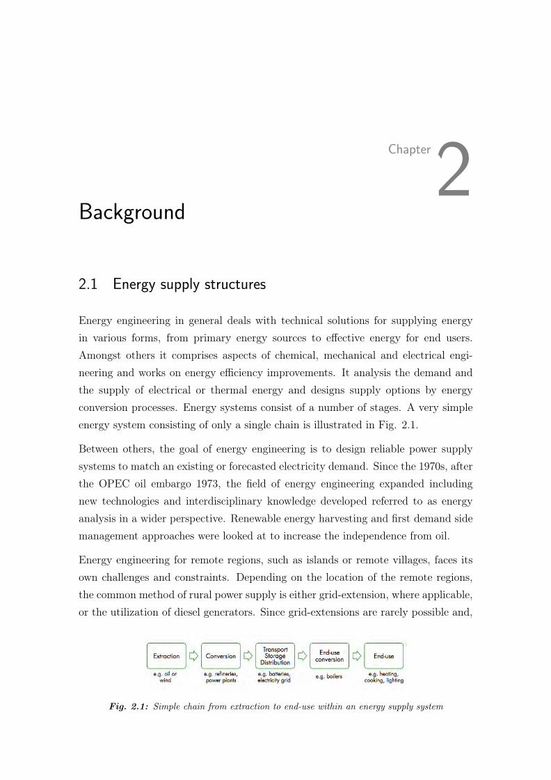
Energy engineering in general deals with technical solutions for supplying energyin various forms, from primary energy sources to effective energy for end users.Amongst others it comprises aspects of chemical, mechanical and electrical engi-neering and works on energy efficiency improvements. It analysis the demand andthe supply of electrical or thermal energy and designs supply options by energyconversion processes. Energy systems consist of a number of stages. A very simpleenergy system consisting of only a single chain is illustrated in Fig. 2.1.
Between others, the goal of energy engineering is to design reliable power supplysystems to match an existing or forecasted electricity demand. Since the 1970s, afterthe OPEC oil embargo 1973, the field of energy engineering expanded includingnew technologies and interdisciplinary knowledge developed referred to as energyanalysis in a wider perspective. Renewable energy harvesting and first demand sidemanagement approaches were looked at to increase the independence from oil.
Energy engineering for remote regions, such as islands or remote villages, faces itsown challenges and constraints. Depending on the location of the remote regions,the common method of rural power supply is either grid-extension, where applicable,or the utilization of diesel generators. Since grid-extensions are rarely possible and,
Fig. 2.1: Simple chain from extraction to end-use within an energy supply system
6 Chapter 2 Background
depending on the distance to the next grid, go usually hand in hand with dispropor-tionately high infrastructure investments, the decentral use of diesel generator setsis widespread practice. However, the consumption of expensive fuel makes them notonly for ecological but also for economic reasons increasingly unattractive [3].
Nowadays in remote regions, energy supply systems including renewable energysources are already able to compete successfully with fossil fuel-powered systems[4, 5]. The main drawbacks of implementing such systems are comparatively highinitial investment costs and limitations when it comes to payback strategies. Islandgrids with a high share of fluctuating energy sources implicate challenges in fre-quency stabilization and require usually a high installed nominal power. To handlethe intermittent character of wind energy, typical approaches for managing fluctua-tion on the supply side are the use of diesel generators for providing operational andcapacity reserve, curtailment of intermittent generation, a distributed generation,complementarity between renewable sources and the integration of energy storages[6]. Therefore such a system has to fulfill following characteristics: It should consistout of relatively small-scale components, some of them have to be flexible in termsof following the load and starting quickly within ten minutes and act as frequencyregulator in combination with an adapted managing system, and black-start-abilityhas to be guaranteed.
Although electricity grids play an essential role in energy system analysis, they arenot addressed within this work. Grid-connection is no possible solution, becausecomplete remoteness is assumed. Electricity grids within considered island systemsare not modeled. Usually all systems require a grid-extension or enhancement andthe required investments are comparable.
2.1.1 Demand Side Management
As mentioned before, first energy engineering approaches under the term DemandSide Management (DSM) came up in the late 1970s. In a number of countries themain approach was and still is to encourage consumers to use less energy duringpeak hours by introducing graded electricity prices [7]. Off-peak times are usuallyat night time and on weekends, that’s why even in some European countries power ischeaper at night than during the day. DSM though has been argued to be ineffectivedue to additional management costs and less effects - measured in insufficient savingsfor utilities.
2.1 Energy supply structures 7
However, in times of an increasing share of renewable energies especially in remoteregions DSM gains in importance. Generally, four different DSM strategies can beidentified [8]:Peak shaving: Utilities manage the customer’s consumption, e.g., by installingdemand-response systems like timers for water heaters in order to reduce peak hourdemand.Valley filling: Off peak loads will be build up to fill times with low demand, forinstance charging electric cars during night time. The goal is to improve the eco-nomic efficiency of a plant or system.Load shifting: This can be accomplished by energy storage systems or deferrableloads. Electrical and thermal storages enable a separation of generation and con-sumption, what can be used excellent for cooling purposes.Conservation The most efficient and obvious way of saving energy, is to reduce theentire energy load by individual savings of every single consumer.
In island grids demand can be managed in various ways, cf. the literature concerningthe integration of renewables e.g. [6, 9]. Within this work, next to electrical andthermal energy storages, the focus is set on the load shifting method of seawaterdesalination as deferrable load. Such a load cannot store electricity, but uses surpluselectricity and minimizes unused dump load increasing the overall efficiency in islandgrids.
2.1.2 Renewable power generation in island grids
Renewable energy conversion technologies could already be integrated successful invarious island grids. Some realized examples in particular are, e.g. Porto Santo,Bonaire or El Hierro.
On Porto Santo, a Portuguese island in the North Atlantic Ocean and part of theMadeira Archipelago, a hybrid wind-diesel utility was installed in 2004. The eco-nomic mainstay on the island is tourism, which comes with high energy demands,in particular for air conditioning. The island has a size of 42 km2 and a populationbetween 5,000 in off-season and 20,000 during tourist season. The hybrid energysystem consists of diesel engine blocks with a total capacity of 10 MW and about900 kW installed wind capacity by Vestas wind turbines. The modular constellationof the system allows a total load coverage of the fluctuating demand on the island.The maximum wind penetration of the system though is limited to 30 % [10].
8 Chapter 2 Background
On the island of Bonaire, Netherlands Antilles, in the Caribbean Sea the world widebiggest wind-diesel-installation was implemented in 2009. About 14,000 people liveon the 288 km2 large island and consume about 205 MWh/day power with a peakload of 11 MW. The planners’ target was to become the first CO2 neutral islandswith twelve wind turbines, each 900 kW, five diesel engines, each 2.5 MW to beoperated on bio-fuel (first imported certified vegetable oil, later locally producedalgae-oil). Based on information by the constructors and planners Enercon, MANand Ecofys, the system operates successfully with a higher share of wind energy thanexpected (about 60 %). On the dry island even a desalination plant is powered bythe hybrid energy supply system.
The Canary islands are also an archipelago with a high ambition to supply powerand water by renewable energy sources and to become independent from fossil fuelimports. El Hierro, one of the Canary islands, supplies electricity for the populationof 10,500 by diesel engines (10.5 MW), a wind farm (11.5 MW) and a pumped-storage hydropower plant (11.3 MW). However, size restrictions on the island are alimiting factor for the feasibility of additional renewable energy projects. The poweris also needed for seawater desalination plants, which consume up to 40 % of thegenerated electricity in peak times. The supply system operates successfully since2011.
A number of further projects to integrate renewable energies into island grids weredeveloped and also realized as reported in the literature, e.g. in [11, 12, 13]. There-fore the implementation of renewable energy technologies in island grids can beconsidered as state-of-the-art.
2.2 Renewable energy technologies 9
2.2 Renewable energy technologies
All renewable energy sources are based on solar energy (solar and wind energy,biomass), the interaction of planet gravitation and planet motion (partly wind, oceanand tidal powers) and the heat stored in the earth. The state-of-the-art of themodeled technologies are presented in the following sections, the ones not modeledbut still relevant in Appendix B.
2.2.1 Photovoltaics
Photovoltaic modules use the photo effect to convert solar radiation immediatelyto electricity (DC). Various cells and modules have been developed and are in use.They can roughly be classified into monocrystalline, polycrystalline and thin filmmodules. Transfer technologies do also exist but have not come out on top untilnow.
Crystalline silicon modules
About 90 % of commercially available photovoltaic modules (PV) are manufacturedout of crystalline silicon slices, so called wafers. Neglecting the introduction ofproduction steps from quartz sand to wafers, from wafers to solar cells and fromsolar cells to modules, the state-of-the-art of PV modules is presented briefly.
The silicon solar-cell production uses the comprehensive experience of the electronicsindustry. Silicon is a so-called indirect semiconductor, whose absorption coefficientfor solar radiation shows relatively low values. Therefore solar cells made of suchsemiconductor material must be relatively thick (at least 50 μm). High layer thick-ness implies high material consumption and thus high costs. They can reach atheoretical maximum efficiency of 30 %. The losses occur due to incomplete useof the solar spectrum and because a part of the absorbed energy is converted toheat instead of electricity. Nevertheless, crystalline silicon is commonly used forphotovoltaic cells, because it is still the best understood material [14].
Common commercial multi-crystalline solar cells (c-Si) reach efficiencies of about16 %, comparable mono-crystalline solar cells 17 to 20 %. The highest efficiencyreached by specifically prepared laboratory cells was 25 %, pretty close to the the-oretical maximum of 30 %. Higher efficiencies can be reached by stacked solar cellsor by concentrating the solar radiation. The efficiency world record for stacked solarcells is short above 40 % but can reach theoretically above 60 % [15]. For reaching
10 Chapter 2 Background
higher voltage and higher currents the solar cells are connected serially and parallellyto modules and are then hermetically enclosed.
Thin-film modules
Already in the 1960s, a multitude of research and development activities have beenconducted to develop cost-efficient thin film solar cells. For this purpose "direct"semiconductors are required. Compared to the wafer-based industry the thin-filmPV industry is about five to seven years behind. Numerous studies show, that thecost reduction potential of thin-film modules is higher than the ones for wafer-basedmodules ever was and due to the flexible material the modules can also be devel-oped to further products. Amorphous silicon (a-Si), for example, discovered in the1970’s, is such a direct semiconductor. Due to the fact that amorphous silicon formsa direct semiconductor, very thin active layers in the range of 1 μm are requiredand very little material is needed. Additionally this process is characterized by verylow deposition temperatures and thus small energy consumption. As a consequencethe costs of solar cell manufacturing are reduced tremendously compared with crys-talline silicon solar cells. Further commonly used thin-film solar cells are based oncadmium-telluride (CdTe) and copper-indium-selenium (CIS). However, comparedto crystalline silicon, thin-film modules do not reach that high efficiencies. Amor-phous solar cells reach up to 13 % in the laboratory (8 to 10 % in mass production),polycrystalline thin films as CdTe and CIS reach up to 16 and 18 % in the labora-tory, commercial solar cells around 11 %. Large thin-film PV power plants, e.g. inGermany, are the plants in Lieberoser Heide with 53 MW (CdTe) installed capacityand Solarpark Buttenwiesen with 1 MW (a-Si) [16]. Despite the low efficiencies, thelower price has a significant impact on investors and decision makers. Inverters andfurther components that would usually be required, are not addressed in detail.
2.2.2 Concentrated Solar Power
Although Concentrated Solar Power (CSP) concepts like DESERTEC (electricitygrids between northern Africa and southern Europe using thermal solar powerplants) are discussed contrary, the technology itself is still a very promising ap-proach using solar radiation for heat production and power generation. Most CSP-technologies are applicable only for large-scale power generation above 10 MWel, butsome have a potential to be used even in island-grids with power demands of under1 MW. In contrast to photovoltaics, CSP can use only the direct, not the diffused
2.2 Renewable energy technologies 11
Fig. 2.2: Parabolic Trough (upper left), Linear Fresnel (bottom left), Solar tower (upper right)and Solar Dish (bottom right) [17]
radiation. Therefore it can only operate at daytime under clear, sunny weatherconditions.
Four main CSP technologies are commercially available or in advanced researchphases. They can be divided into two main groups: linearly focusing and punctuallyfocussing plants. The two linearly focussing CSP technologies are Parabolic Troughand Linear Fresnel, the two punctually focusing ones the Solar Tower and the SolarDish, cf. Fig. 2.2 [17]. The high-temperature heat is provided for electricity gener-ation with conventional power cycles using steam turbines, gas turbines or Stirlingengines. Most systems use glass mirrors for concentration, which continuously trackthe position of the sun. The solar receiver’s coating has usually a high radiationabsorption coefficient and a low reflectivity. It contains a heat transfer fluid, e.g.water, oil or molten salt that takes the heat towards a thermal power cycle, wherehigh pressure or high temperature steam is generated to drive a turbine.
In a standard electricity generation system of parabolic troughs the solar collec-tor assembly has a total length of around 150 meters. It consists of several solarcollectors connected to a single axis sun tracking system. Parabolic troughs are themost mature CSP technologies. The common heat transfer fluid is thermal oil, thecommon steam parameters are 370◦C at 100 bar. For periods when the sun is notshining thermal energy storages can be used as backup system [18]. The parabolicdish, or dish Stirling technology is combined with a Stirling engine. The surfaceof the dish is covered by mirrors, which reflect light into the receiver. This receiver
12 Chapter 2 Background
can be an engine, vessel or box located at the focal point of the parabola. The fluidis heated up to 750◦C and electricity is generated. Solar dishes offer the highestsolar-to-electric conversion performance of all CSP systems. Other features of thisdesign are the compact size, the option of small capacity installations, a systemdesign without cooling water, but the same time a low compatibility with thermalenergy storages [19, 20].In a central tower installation, also called solar tower, an array of heliostats (suntracking mirrors) acts as the solar collector, concentrating solar radiation onto acentral receiver located at the top of a tower. Like in the other methods air or atransfer fluid is being heated, which in turn is used for electricity generation [21].Compared to parabolic troughs, linear Fresnel reflectors have the advantage of asimple and less expensive design, due to linear instead of bended mirrors. Directsteam generation can also be achieved easier than at parabolic through systems,where usually heat transfer fluids and heat exchangers are needed. On the otherhand, Fresnel plants are less efficient and it is more difficult to combine their designwith thermal energy storages.
An option to use CSP in smaller dimensions is to apply an organic working fluidwith a low boiling point in a Clausius Rankine Cycle, also called Organic Rankine
Cycle (ORC). Due to the low boiling point of the fluid, lower temperatures andsmaller plant dimensions are sufficient for electricity generation. Such a plant canoperate in a power range from a few kW up to 10 MW. Low temperature levels thoughalso mean, that by relaxing the steam the gainable enthalpy difference and thereforethe overall efficiency is relatively low. Up to now ORC processes are mainly usedfor geothermal energy conversion, combustion of biomass and waste heat recovery.First research approaches investigate chances of combining ORC processes with CSP[22, 23].
High investment costs are the bottleneck of concentrating solar power plants. Al-though current developments do not prove this tendency, some studies predict asignificant decrease of investment costs, due to learning curves, economies of scaleand technical innovation [24, 25, 26]. A clear advantage of the thermal solar powertechnology is the possibility to store high temperature ( > 120◦C for power gener-ation) as well as low temperature thermal energy, which is significantly easier andcheaper than to store electrical energy. This way power can be supplied also aftersunset for three to eight hours. An overview of applicable thermal energy storage sys-tems is given in section 2.3. Detailed technological data concerning the efficiencies,
2.2 Renewable energy technologies 13
capacities etc., are presented in Tab. 5.2 in section 5.4, where all input parameterare introduced.
2.2.3 Wind energy converters
Wind energy utilization is one the most established renewable energy conversiontechnologies. Humans have used windmills since at least 200 B.C. for grinding grainand pumping water. The theoretical maximum overall efficiency of wind energy con-verters (WECs) is capped with the Betz power coefficient of 59.3 %. Commerciallyavailable wind energy converters transform 30 to 45 % of the energy contained inundisturbed wind into electric power. A wind turbine can differ in a number ofcharacteristics. Today the most common turbine configuration is using a horizontalaxis. It consists of a tall tower, a fan-like rotor on the top that faces into or awayfrom the wind, a generator, a controller, and other components. Most horizontalaxis turbines built today are three-bladed. WECs have different dimensions andrated powers depending on the requirements from 10 kW up to 5 MW per windturbine and differ mainly in the manufacture process and the used materials. Themost important features of various state-of-the-art technologies include:
• rotor axis position (horizontal, vertical),• number of rotor blades (one, two, three or multiple blade rotors),• speed (high and low speed energy converters),• number of rotor revolutions (constant or variable),• upwind or downwind rotors,• power control (stall or pitch control),• wind resisting strength (wind shielding or blade adjustment),• gearbox (converters equipped with gearbox or gearless converters),• generator type (synchronous, asynchronous or direct current generator),• grid connection for power generation plants (direct connection or connection
via an intermediate direct current circuit) [27].
For remote regions with a peak power demand of only a few megawatt or even underone megawatt, only small wind energy converters are applicable. Whereas at themegawatt level only horizontal axis installations can be installed, for small-scaleapplications occasionally also vertical ones can be employed. Independently fromload profiles, sometimes the installation of small wind turbines is required becauseof shipping difficulties in small harbours or installation restrictions for heavy andlarge-sized equipment. Small to medium scale wind turbines under 300 kW though
14 Chapter 2 Background
are not available that common due to the upscaling process at more and moremanufacturers.
What also needs to be considered is the meteorological background. In hurricaneregions, e.g. the Caribbean, only hurricane-proofed wind turbines can be erected.Some manufacturers (like Enercon) do not deliver in hurricane regions, others endurewind speeds of about 70 m/s and can be folded and lowered to the ground in caseof hurricane or cyclone warnings. All detailed information of modeled wind turbinesare presented in section 5.4.
2.3 Energy storage systems
2.3.1 Thermal energy storage systems
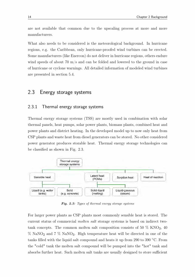
Thermal energy storage systems (TSS) are mostly used in combination with solarthermal panels, heat pumps, solar power plants, biomass plants, combined heat andpower plants and district heating. In the developed model up to now only heat fromCSP plants and waste heat from diesel generators can be stored. No other consideredpower generator produces storable heat. Thermal energy storage technologies canbe classified as shown in Fig. 2.3.
Fig. 2.3: Types of thermal energy storage systems
For larger power plants as CSP plants most commonly sensible heat is stored. Thecurrent status of commercial molten salt storage systems is based on indirect two-tank concepts. The common molten salt composition consists of 50 % KNO3, 40% NaNO2 and 7 % NaNO3. High temperature heat will be directed in one of thetanks filled with the liquid salt compound and heats it up from 290 to 390 ◦C. Fromthe "cold" tank the molten salt compound will be pumped into the "hot" tank andabsorbs further heat. Such molten salt tanks are usually designed to store sufficient
2.3 Energy storage systems 15
heat for electricity generation for six to eight hours. Heat losses are assumed tobe 1 ◦C per day and tank [17]. The molten salt storage test facility of DLR inCarboneras, Spain, e.g., has a storage capacity of 1 MWh, is kept under a steampressure of 100 bar and can bear a maximum temperature of 500 ◦C. Temperaturesin molten salt tanks need be be kept above 250 ◦C. As soon as the salt compoundcrystallizes, its storage capability freezes and the storage cannot be used anymore.Therefore when a molten-salt storage is not needed anymore, it can be cooled downand removed in a crystalline form. Molten salt storage systems show a limitedpotential for further cost reductions [28].
A further sensible heat storage is concrete: The basic module of a pilot plant inANDASOL 1 in Granada, Spain, can store 5 MWh and has a temperature stabilityof up to 500 ◦C. From the solar collectors heated oil of 400 ◦C flows in parallel pipesthrough the concrete and heats it up. In case of discharge the oil disperses againthrough further pipes with a temperature of around 350 ◦C and produces through aheat exchanger steam for driving the generator. Concrete storages are usually alsodesigned to store thermal energy for six to eight hours. Solid media storage systemsrepresent a cost effective approach for medium and high temperature applications.Current investment costs are less than the ones for molten salt with around 35e/kWh [17].
Latent heat storage units are usually low temperature storages used for smallerenergy capacities than the ones discussed before. Steam cycles and phase changematerials (PCMs) are the most common latent heat storage approaches. The basicprinciple of steam accumulators is, that sensible heat is stored in pressurized liquidwater. Water is stored in an isolated pressure vessel in liquid and steam phase.Charging and discharging can generally occur in the liquid and in the steam phase.Latent heat storage by PCMs can principally be achieved through solid-liquid, solid-gas or liquid-gas phase changes. However, the only phase change used for PCMs isthe solid-liquid one, because changes to the gas phase would require high pressuresor large volumes. Commonly used organic PCMs are paraffins and fatty acids orinorganic salt hydrates. The feasibility of latent heat storage systems though hasbeen demonstrated also for high temperatures up to 300 ◦C in the MW-range [28].Aquifers and other heat storages are also possible solutions but not addressed in theframework of this study.
16 Chapter 2 Background
2.3.2 Electricity storage systems
Numerous electricity storage technologies (ESS) are in use. For micro-grids witha high share of renewable energy sources other storages are needed than for small-scale stand-alone systems or large interconnection grids. In isolated distributionnetworks, like the ones discussed here, the fluctuating character of most renewableenergy technologies makes the usage of electricity storages indispensable.
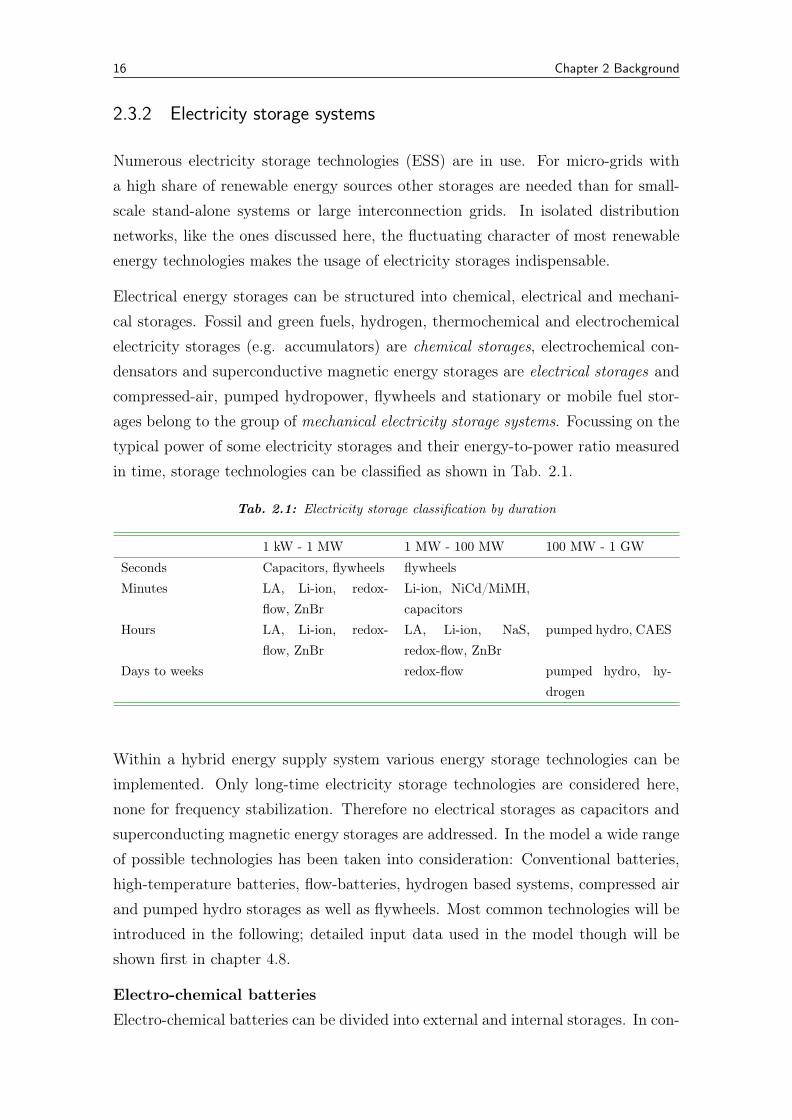
Electrical energy storages can be structured into chemical, electrical and mechani-cal storages. Fossil and green fuels, hydrogen, thermochemical and electrochemicalelectricity storages (e.g. accumulators) are chemical storages, electrochemical con-densators and superconductive magnetic energy storages are electrical storages andcompressed-air, pumped hydropower, flywheels and stationary or mobile fuel stor-ages belong to the group of mechanical electricity storage systems. Focussing on thetypical power of some electricity storages and their energy-to-power ratio measuredin time, storage technologies can be classified as shown in Tab. 2.1.
Tab. 2.1: Electricity storage classification by duration
1 kW - 1 MW 1 MW - 100 MW 100 MW - 1 GW
Seconds Capacitors, flywheels flywheelsMinutes LA, Li-ion, redox-
flow, ZnBrLi-ion, NiCd/MiMH,capacitors
Hours LA, Li-ion, redox-flow, ZnBr
LA, Li-ion, NaS,redox-flow, ZnBr
pumped hydro, CAES
Days to weeks redox-flow pumped hydro, hy-drogen
Within a hybrid energy supply system various energy storage technologies can beimplemented. Only long-time electricity storage technologies are considered here,none for frequency stabilization. Therefore no electrical storages as capacitors andsuperconducting magnetic energy storages are addressed. In the model a wide rangeof possible technologies has been taken into consideration: Conventional batteries,high-temperature batteries, flow-batteries, hydrogen based systems, compressed airand pumped hydro storages as well as flywheels. Most common technologies will beintroduced in the following; detailed input data used in the model though will beshown first in chapter 4.8.
Electro-chemical batteries
Electro-chemical batteries can be divided into external and internal storages. In con-
2.3 Energy storage systems 17
trast to internal ones, for external storages (e.g. flow batteries) the power unit canbe dimensioned separately from the storage capacity. Internal electro-chemical stor-ages can be further divided into low-temperature and high-temperature ones. Low-temperature storages for example are the lead-acid, nickel-cadmium and lithium-ionbatteries requiring an ambient temperature of about 20 ◦C, high-temperature stor-ages, like the sodium-sulphur battery for example, require a nominal temperature ofabove 250 ◦C.
Lead-acid batteries:
Conventional lead-acid batteries (LA) used for over a century are usually used forsmall but also several large applications. Low investment costs and relatively highefficiencies make this battery attractive. However, its low cycle lifetime and poorperformance at extreme temperatures makes these batteries vulnerable. There areclosed low-maintenance and open high-maintenance LA batteries. During chargingprocesses and excessive charge hydrogen frees up. In open LA batteries water refill-ing (every three to six months) compensates the losses, in closed LA batteries thehydrogen recombines within the battery and pressure control valves are integrated,so called Valve-Regulated Lead-Acid (VRLA) batteries. VRLA batteries are almostmaintenance-free but are more expensive.
Nickel batteries:
The Nickel-electrode batteries, and in particular the nickel-cadmium devices (NiCd)have a high specific energy and require little maintenance, but have high costs anda relatively low cycle life. Compared to lead-acid, these batteries are robust againstextreme conditions and can be fully discharged without capacity and efficiency lossesand without minimizing its cycle life. Since cadmium though is toxic, NiCd-batteriesare not further considered (e.g. in Germany, their usage is prohibited.) Nickel-metalhydride batteries (NiMH) are the advanced batteries [29].
Lithium-ion batteries:
Li-ion battery installations have a significantly higher power density and energydensity than lead-acid batteries and have a high application range. However, forstationary applications the cost per kilowatt hour stored is comparatively high anddepending on the required capacity, it is not first choice for stationary applications[30].
Sodium-sulphur batteries:
Sodium-sulphur systems (NaS) are categorized as high-temperature batteries op-erating at temperatures around 300 ◦C. Since their electrodes are both molten,sometimes they are also called "molten salt" devices. Their specific energy is three
18 Chapter 2 Background
to four times higher than the one of lead-acid batteries, they have a strong life cycleperformance, decent energy efficiencies and are able to provide high power burstswhich make them applicable also for frequency stabilization purposes. Maintenanceis required every three years. Further details can be seen in Tab. 5.5 in section 5.4.
Redox-flow batteries:
Redox-flow batteries differ from the previously presented batteries by the fact thatthe electro-chemical conversion is separated from the storage unit. The power ca-pacity and energy capacity can be scaled independently. The electrolyte (storagemedium) is stored in external tanks and will be pumped into the power unit ac-cording to requirements. There the electrolyte will be charged or discharged. Thepower performance depends on the power unit, the storage capacity on the size ofthe tanks. The efficiency of the system is quite low due to the pumping require-ments. Redox-flow batteries are optimal for long-term energy storage as it can bedesigned to achieve very low self-discharge rates when the system is in standby. Afurther benefit of this system design is that complete discharges of the battery (100 %depth-of-discharge) are not damaging the battery, but even improve its performance.These systems have a long lifetime and typically only individual components needto be replaced, such as the stacks, while the electrolyte can be used indefinitely [31].Typical redox-flow battery designs are the Vanadium redox battery (V-redox), thePolysulfide-bromide battery, and the zinc-bromine battery (ZnBr). The Polysulfide-bromide battery was commercially produced under the name Regenesys and per-formed best. The technology was bought though by RWE, the licenses were soldand the project abandoned. The most common flow battery is the Vanadium-Redox-Flow battery and its most present producer is Cellstrom. Zinc-bromine batteries arerelatively new on the market and are only partly a flow battery. They are suitedin applications that require deep cycle and long cycle life energy storage. There arestill difficulties at the charging process, because zinc forms dendrites on the electrodethat can form short circuiting pathways [29].
Hydrogen:
Hydrogen-based systems can only be considered as energy storage technologies ifthe production and storage of hydrogen is part of the overall system. Hydrogencan be generated by electrolysis of water and stored either cooled down to 20.28K (-253 ◦C) as liquid or as pressurized gas in a tank. For power generation twomain approaches are used: fuel cells or combustion engines. Fuel cells, as the protonexchange membrane (PEM) cells, have the advantage to operate with hydrogen andair at ambient temperatures with good time response and relatively high efficiencies.
2.3 Energy storage systems 19
Also common is to burn the hydrogen in a combustion engine. Diesel engines havealready been modified for this task and produce electricity at a quite high efficiencywith the advantage of a relatively inexpensive power generation section [30]. Furtherdevelopments are solar fuel systems as the methane battery, commercialized bySolar Fuel Technology GmbH and Co KG. Here hydrogen is further converted intomethane.
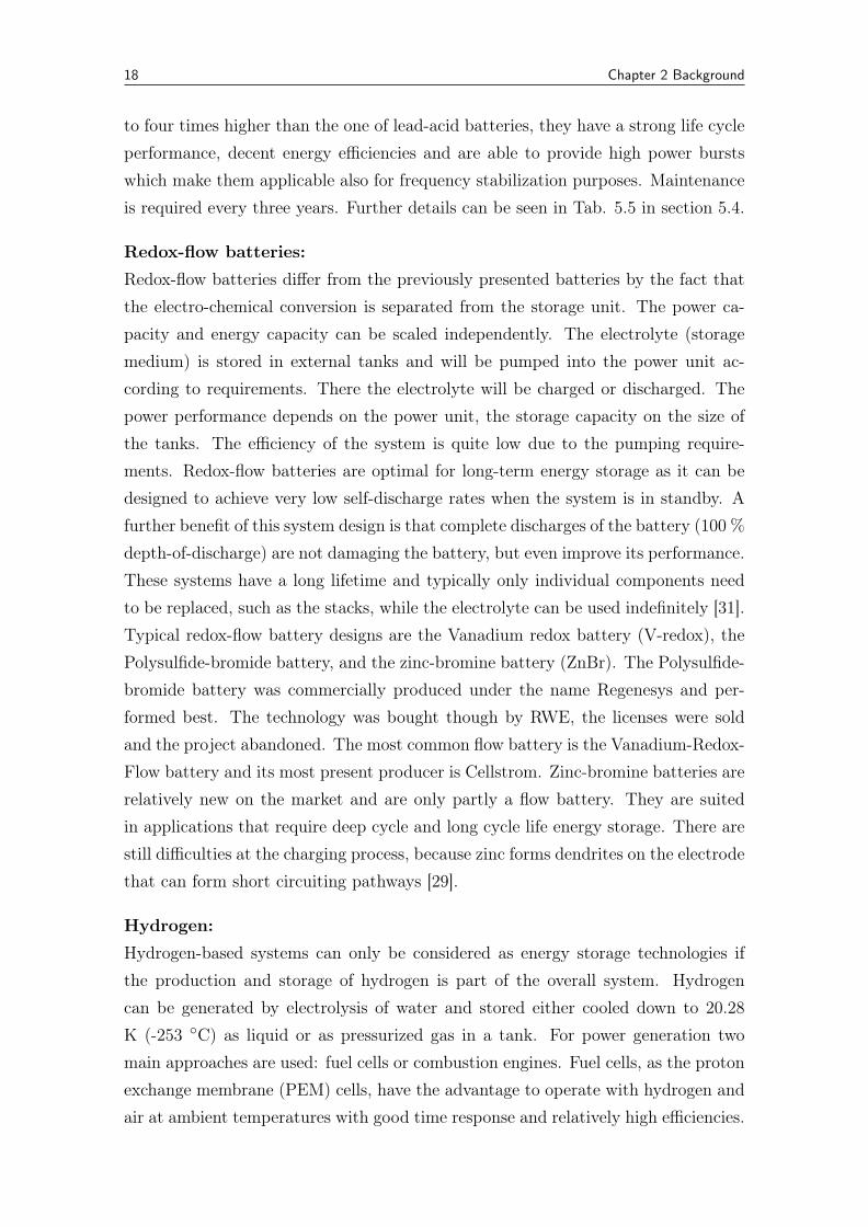
The Ragone plot shows some of the mentioned electrochemical storage devices char-acterized by their energy density over their power density. Capacitors as shownhere for frequency stabilization are not addressed in detail, but the properties ofcommonly used lead-acid and lithium-ion batteries are demonstrative for stationaryenergy storage systems. The not depicted NaS high-temperature battery is maybethe most flexible battery, being able to operate as flexible load control but also aslong-term storage system.
Fig. 2.4: Ragone Diagram of electrochemical storages
20 Chapter 2 Background
Mechanical ESS
Compressed-air energy storage:
The traditional compressed-air energy storage (CAES) uses geologic formations inthe underground for storing air under high pressured. CAES systems have efficienciesof 50-55 % and can perform in part-load until minimum 20 %. They are essentiallygas turbine plants where the air is already compressed and therefore less fuel isconsumed [32]. Because of their similarity to standard gas turbine systems, theyare easily to integrate into existing power networks. With a ramp rate similarand slightly faster than traditional gas turbine plants, these systems are ideal formeeting peak loads. For island systems as the ones discussed in this work, suchbig installations are not applicable. There are some small compressed air energystorage systems available, where the compressed air is stored in steel pipes that aretypically used for natural gas transmission. These pipes are relatively inexpensiveand are generally available [31]. Since no specific geological formations are required,such systems allow a higher flexibility in siting than conventional CAES. If thecompression heat is not cooled down but stored in an additional heat energy storage(adiabatic CAES), the efficiency can increase up to 70 %.
Pumped hydroelectric storage:
Pumped hydroelectric storages (PHS) are based on conventional hydropower tech-nology. Hydropower requires a considerable volume of water to generate electricity,approximately V[m3] = 400 · E[kWh]
h[m] . A PHS consists of a pumping turbine, a motor-generator-unit, a lower and a higher reservoir. The simple design and the experiencewith hydropower plants has made PHS the standard energy storage design for a cen-tury. These systems can ramp up to full load in a few seconds. Plants have a powerrange from a few megawatt up to one gigawatt and a durability from usually 50 years[33]. However, they require very specific geographic features that limit the siting ofsuch plants. PHS require relatively low maintenance but high initial investments.PHS projects also face criticism due to their significant impact on local wildlife,ecosystems, and landscape.
Flywheel:
Flywheels have been in existence for centuries, however, only over the past fewdecades they have been considered as forms of bulk energy storage. They storekinetic energy. These systems are extremely rapid in their response time and, withrecent developments in bearing design, have been able to achieve high efficiencies forshort durations of storage. Their main disadvantages are a high rate of self discharge
2.4 Backup system 21
due to frictional losses and their relatively high initial costs. Flywheels are durablewithout significant replacement needs [34]. Although flywheels are occasionally alsodiscussed as stationary storages, they are not considered in this study. High selfdischarge rates are not acceptable for long-term stationary storages.
2.4 Backup system
For the case that renewable energy sources cannot serve the load and the energystorage is empty, a backup system is required for guaranteeing a reliable energysupply. As backup system usually diesel generator sets are applied, since in manycases such a power station has provided the remote region with electricity previously.Stationary generator sets use usually diesel oil as fuel. As far as local conditionsallow, diesel oil can be complemented with biodiesel. In case of the goal of renewableenergy maximization, a 100 % share of renewables energy sources is not achievableanother way. Depending on the utilization of a existent diesel generator or a newone and the share of renewables, the nominal capacity of such a backup systemcan operate far outside of the optimum. If the diesel generator used to meet thewhole power demand, it will probably not operate that efficient in part-load andtwo diesel generators with lower nominal capacities could be beneficial. In systemdesigns though commonly the peak demand is taken as nominal capacity of thebackup diesel generator, not taking into account periods of part-load operation.This depends though on the dispatch strategy, if the diesel generator is operatingload following or cycle charging. If it runs cycle charging, it operates at full load atthe technical optimum and charges the batteries with the surplus electricity. In thegiven model a load following dispatch strategy is assumed. The cold-start-up time ofa generator is usually about ten minutes and therefore flexible enough to be activatedin case of low wind speeds or low solar radiation predictions. Part-load operationis usually limited to minimal 30 or 50 % of the nominal capacity. Commonly upto 1000 activations per year can be carried out by a diesel generator engine. Theminimal duty-cycles have been set to three hours in the model. Specific load curvesare presented in section 5.4, when the used input data will be introduced.

22 Chapter 2 Background
2.5 Seawater desalination in remote regions
2.5.1 Basics of water
Clean freshwater is globally a precious commodity. The World Health Organisationreports that 1 billion people do not have access to clean drinking water. Uncleandrinking water is responsible for millions of water related illnesses and billions ofdollars in health care costs. As a result of population growth, the sinking qual-ity of existing water resources, the increasing industrial and agricultural demands,climate change, and the dissipation of clean water, resources are overused. Globaldesertification and excessive usage of natural freshwater reservoirs diminish accessi-ble water stocks. Within the next two decades it is assumed that about one-thirdof the world’s population will suffer serious water scarcity problems [35].
Since water usage is hard to describe, the water footprint and virtual water content ofagricultural and industrial products was introduced in the late 1990s. For example,to harvest 1 kg rice up to 3000 liters of water are needed, for 1 sheet A4 paper10 liters, for 1 pair of shoes (bovine leather) 8000 liters [36]. The daily per capitause of water in average in different residential areas are, e.g. 150 liters in the theEuropean Union, 300-350 liters in the USA and Japan, 800 liters in the UnitedArabian Emirates, but only 10-20 liters in sub-Saharan Africa [35].
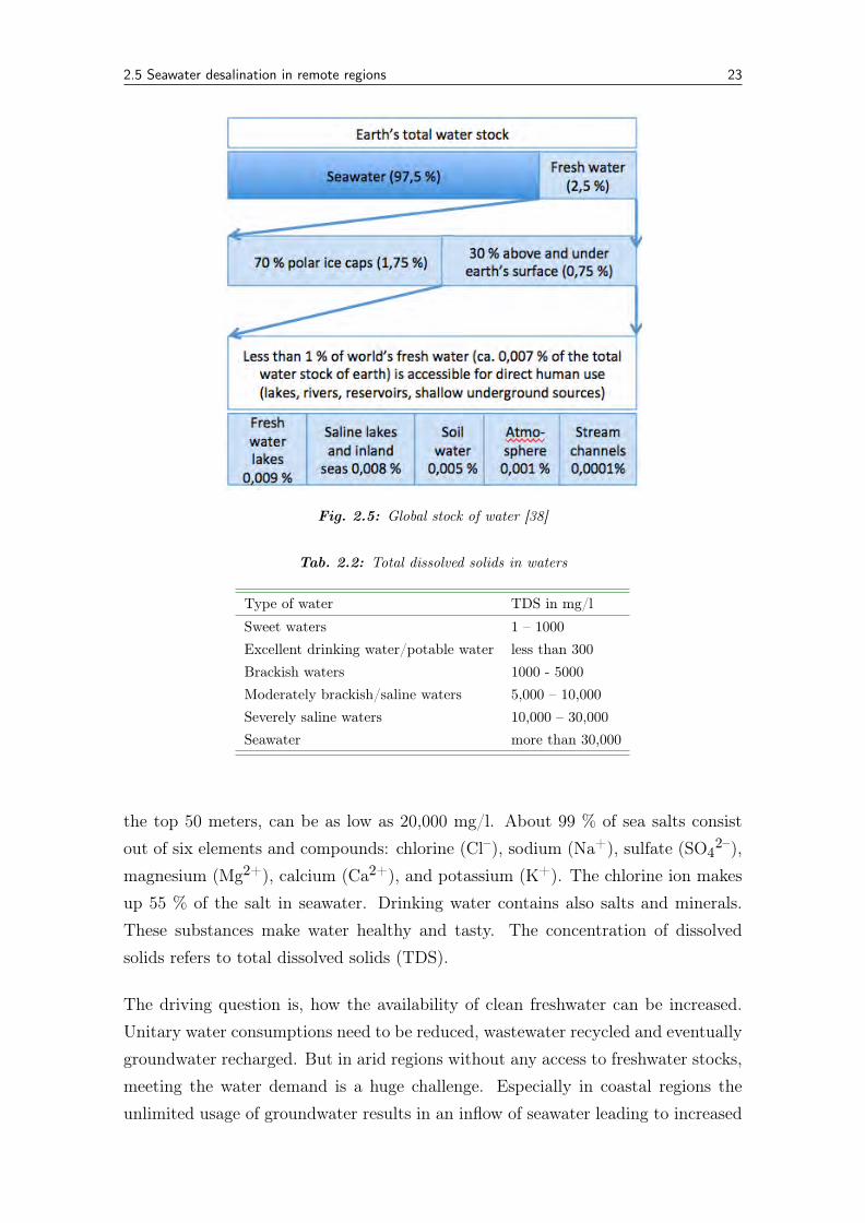
Worldwide, agriculture accounts for 70 % of all water consumption, compared to20 % for industry and 10 % for domestic use. In industrialized nations, however,industry consumes more than half of the water available for human use. Belgium,for example, uses 80 % of the water for industry [37]. A basic reason for waterscarcity is the fact, that only a small fraction of all water on earth is freshwater, themain part is salty seawater. Figure 2.5 shows that only 2.5 % (35 million m3) of theworld’s water resources is freshwater, the rest (13 million m3) is salty and thereforenot usable for human consumption or industrial purposes [38].
The water quality and type can be differentiated depending on the salt content.Even in ocean basins the salt concentration differs due to regional freshwater losses(evaporation) and gains (runoff and precipitation). Table 2.2 gives an overview ofvarious waters and their denotation.
Typically, seawater has a salinity of 35,000 mg/l. The Arabian Gulf though, forexample, has an average salt content of 48,000 mg/l and the salinity of the DeadSea reaches even 250,000 mg/l. The same time the salinity of the Arctic Ocean, i.e.
2.5 Seawater desalination in remote regions 23
Fig. 2.5: Global stock of water [38]
Tab. 2.2: Total dissolved solids in waters
Type of water TDS in mg/l
Sweet waters 1 – 1000Excellent drinking water/potable water less than 300Brackish waters 1000 - 5000Moderately brackish/saline waters 5,000 – 10,000Severely saline waters 10,000 – 30,000Seawater more than 30,000
the top 50 meters, can be as low as 20,000 mg/l. About 99 % of sea salts consistout of six elements and compounds: chlorine (Cl–), sodium (Na+), sulfate (SO4
2–),magnesium (Mg2+), calcium (Ca2+), and potassium (K+). The chlorine ion makesup 55 % of the salt in seawater. Drinking water contains also salts and minerals.These substances make water healthy and tasty. The concentration of dissolvedsolids refers to total dissolved solids (TDS).
The driving question is, how the availability of clean freshwater can be increased.Unitary water consumptions need to be reduced, wastewater recycled and eventuallygroundwater recharged. But in arid regions without any access to freshwater stocks,meeting the water demand is a huge challenge. Especially in coastal regions theunlimited usage of groundwater results in an inflow of seawater leading to increased
24 Chapter 2 Background
salt levels making the freshwater unfit for human consumption and other applica-tions. Globally desalination is increasingly used for reducing current or future waterscarcity, especially in coastal areas [37].
When looked at from an environmental perspective, desalinating seawater can be anecological friendly solution if the usage of fossil fuels and the emission of chemicalsin the brine is minimized. The combination with highly developed renewable energytechnologies can be a chance to minimize at least the emission of greenhouse gases.Numerous remote regions with no access to natural freshwater reservoirs are char-acterized by high solar irradiance and good wind conditions. To understand betterthe options of combining renewable energy systems with desalination technologies,in the following an overview of the main desalination processes is given.
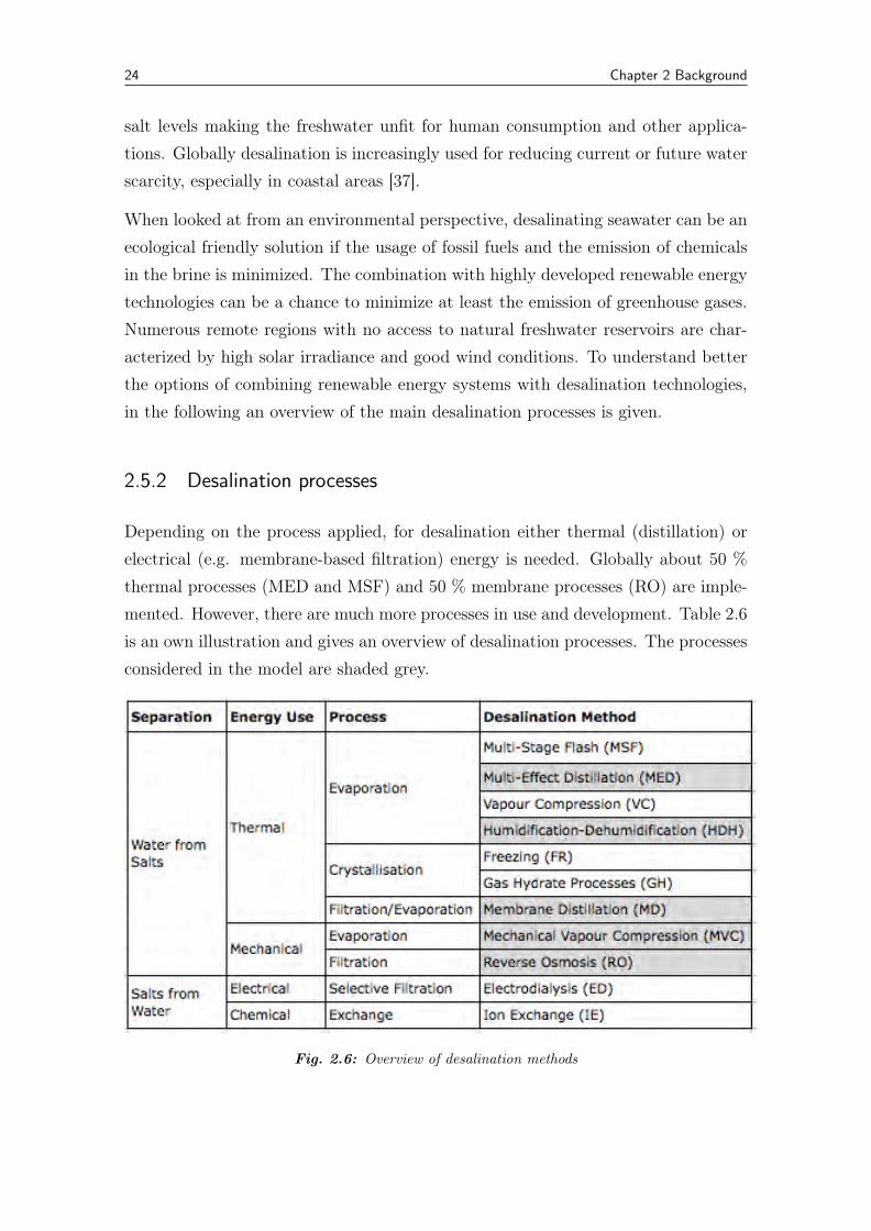
2.5.2 Desalination processes
Depending on the process applied, for desalination either thermal (distillation) orelectrical (e.g. membrane-based filtration) energy is needed. Globally about 50 %thermal processes (MED and MSF) and 50 % membrane processes (RO) are imple-mented. However, there are much more processes in use and development. Table 2.6is an own illustration and gives an overview of desalination processes. The processesconsidered in the model are shaded grey.
Fig. 2.6: Overview of desalination methods
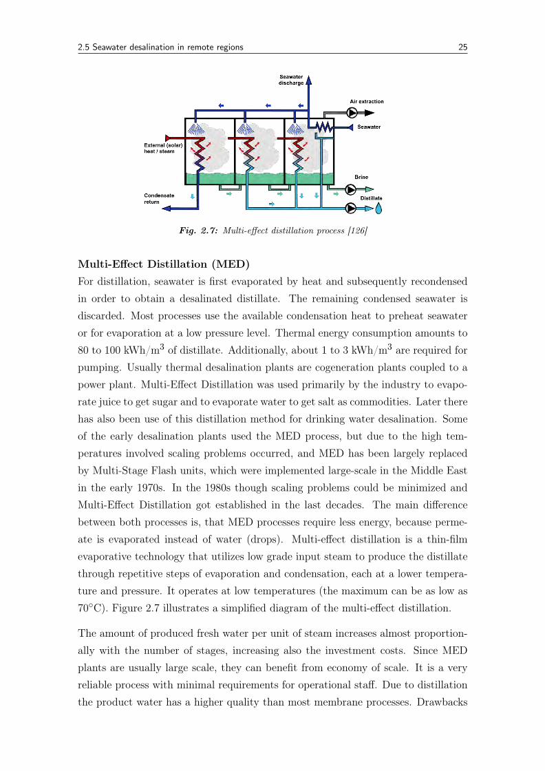
2.5 Seawater desalination in remote regions 25
Fig. 2.7: Multi-effect distillation process [126]
Multi-Effect Distillation (MED)
For distillation, seawater is first evaporated by heat and subsequently recondensedin order to obtain a desalinated distillate. The remaining condensed seawater isdiscarded. Most processes use the available condensation heat to preheat seawateror for evaporation at a low pressure level. Thermal energy consumption amounts to80 to 100 kWh/m3 of distillate. Additionally, about 1 to 3 kWh/m3 are required forpumping. Usually thermal desalination plants are cogeneration plants coupled to apower plant. Multi-Effect Distillation was used primarily by the industry to evapo-rate juice to get sugar and to evaporate water to get salt as commodities. Later therehas also been use of this distillation method for drinking water desalination. Someof the early desalination plants used the MED process, but due to the high tem-peratures involved scaling problems occurred, and MED has been largely replacedby Multi-Stage Flash units, which were implemented large-scale in the Middle Eastin the early 1970s. In the 1980s though scaling problems could be minimized andMulti-Effect Distillation got established in the last decades. The main differencebetween both processes is, that MED processes require less energy, because perme-ate is evaporated instead of water (drops). Multi-effect distillation is a thin-filmevaporative technology that utilizes low grade input steam to produce the distillatethrough repetitive steps of evaporation and condensation, each at a lower tempera-ture and pressure. It operates at low temperatures (the maximum can be as low as70◦C). Figure 2.7 illustrates a simplified diagram of the multi-effect distillation.
The amount of produced fresh water per unit of steam increases almost proportion-ally with the number of stages, increasing also the investment costs. Since MEDplants are usually large scale, they can benefit from economy of scale. It is a veryreliable process with minimal requirements for operational staff. Due to distillationthe product water has a higher quality than most membrane processes. Drawbacks
26 Chapter 2 Background
of the technology are the high thermal energy demand, cf. Tab. 5.7 later on) andhigh capital costs, since due to corrosion high quality materials are required [39].Corrosion is also avoided by adding appropriate chemicals. These though are harm-ful for the environment and are usually flushed into the sea. Extensive research isundertaken for realizing zero-liquid-discharge. Distillation processes like MSF andMED usually are robust and need only a crude filtration, other than membranetechnologies, which depend on the incoming feed water quality and require morechemical pre-treatment.
Most of the almost 900 MED-plants worldwide, mainly located in the Middle East,the Caribbean, India and Southern Europe use a number of 8 to 16 effects andproduce usually 50,000 to 800,000 m3 of freshwater per day. Down-scaling is notbeneficial from an economic perspective. The demand of mid-scale desalinationplants in the range of 500 to 10,000 m3/day is increasing though, e.g. for industrialpurposes and smaller urban regions, and even one, two and three effect technologiesare tried to be commercialized, e.g in El Gouna, Egypt.
Humidification-Dehumidification (HDH)
A further thermal desalination process is the humidification-dehumidification method.HDH is more a small-scale application, producing 50 to 500 m3/day. The processrequires also mainly thermal energy, e.g. waste heat from combustion processes orsolar thermal heat, in the range of 50 to 95 ◦C and 1 to 3 kWhel/m3 for the pumps.Figure 2.8 illustrates a simplified process scheme. The heat source in this case is asolar collector, heating the incoming seawater, which is previously pumped throughthe condenser and acts as the coolant in the heat-exchange process of the system.The heated seawater is sprayed into the evaporation chamber, where it enriches dryair with vapour. The air circulates by natural or forced convection. The humidifica-tion of the dry air is based on the principle of mass diffusion. The vapour carryingcapability of air increases with the temperature, e.g. 1 kg of dry air saturated withvapour can carry additional 0.26 kg of water vapour (about 208 kJ/kg) when its tem-perature increases from 30 to 80◦C. When the enriched air reaches the condenserwith the circulating cold seawater as coolant, it dehumidifies. The delivered distil-late is collected at the condenser, while the brine is separated in the evaporator.The brine can be concentrated so high, that zero-liquid-discharge is a reachable goalfor this process [40].
A further advantage of HDH is the simple, robust and relatively cheap construc-tion. Some manufacturers use no steel at all, only plastics as polyvinyl chloride,which guarantees a corrosion-free process and low maintenance. Since no filters
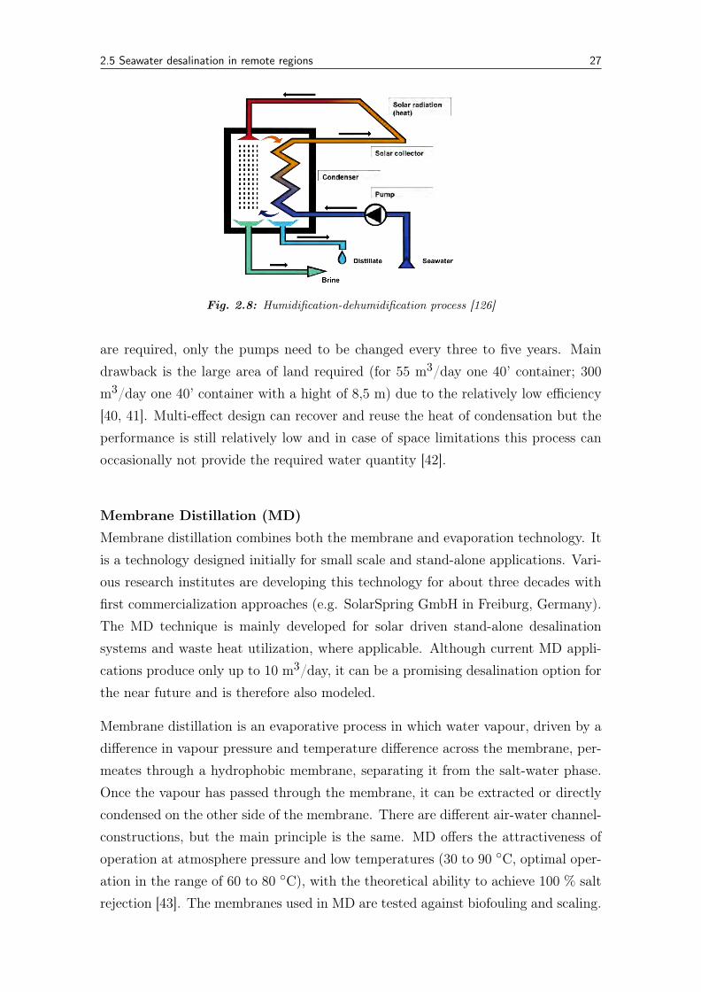
2.5 Seawater desalination in remote regions 27
Fig. 2.8: Humidification-dehumidification process [126]
are required, only the pumps need to be changed every three to five years. Maindrawback is the large area of land required (for 55 m3/day one 40’ container; 300m3/day one 40’ container with a hight of 8,5 m) due to the relatively low efficiency[40, 41]. Multi-effect design can recover and reuse the heat of condensation but theperformance is still relatively low and in case of space limitations this process canoccasionally not provide the required water quantity [42].
Membrane Distillation (MD)
Membrane distillation combines both the membrane and evaporation technology. Itis a technology designed initially for small scale and stand-alone applications. Vari-ous research institutes are developing this technology for about three decades withfirst commercialization approaches (e.g. SolarSpring GmbH in Freiburg, Germany).The MD technique is mainly developed for solar driven stand-alone desalinationsystems and waste heat utilization, where applicable. Although current MD appli-cations produce only up to 10 m3/day, it can be a promising desalination option forthe near future and is therefore also modeled.
Membrane distillation is an evaporative process in which water vapour, driven by adifference in vapour pressure and temperature difference across the membrane, per-meates through a hydrophobic membrane, separating it from the salt-water phase.Once the vapour has passed through the membrane, it can be extracted or directlycondensed on the other side of the membrane. There are different air-water channel-constructions, but the main principle is the same. MD offers the attractiveness ofoperation at atmosphere pressure and low temperatures (30 to 90 ◦C, optimal oper-ation in the range of 60 to 80 ◦C), with the theoretical ability to achieve 100 % saltrejection [43]. The membranes used in MD are tested against biofouling and scaling.
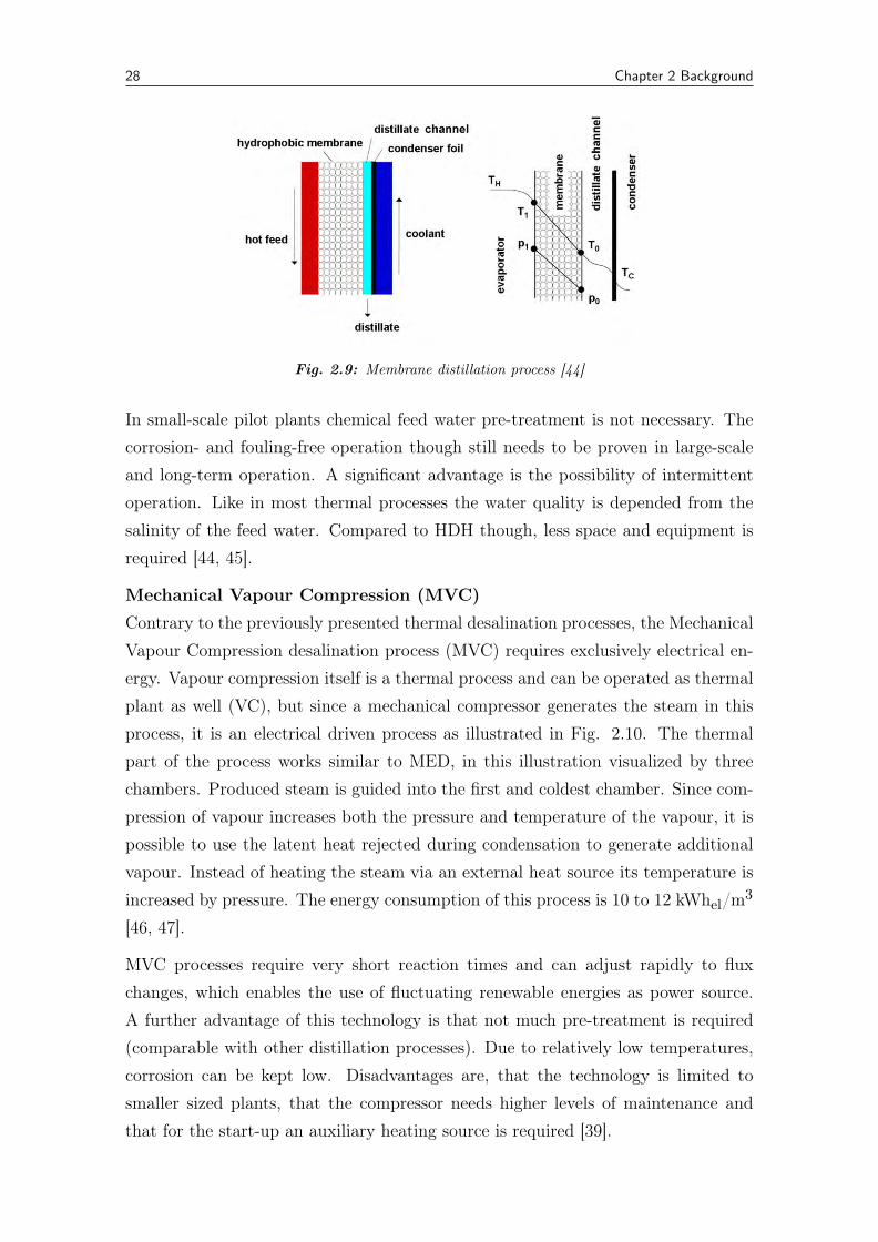
28 Chapter 2 Background
Fig. 2.9: Membrane distillation process [44]
In small-scale pilot plants chemical feed water pre-treatment is not necessary. Thecorrosion- and fouling-free operation though still needs to be proven in large-scaleand long-term operation. A significant advantage is the possibility of intermittentoperation. Like in most thermal processes the water quality is depended from thesalinity of the feed water. Compared to HDH though, less space and equipment isrequired [44, 45].
Mechanical Vapour Compression (MVC)
Contrary to the previously presented thermal desalination processes, the MechanicalVapour Compression desalination process (MVC) requires exclusively electrical en-ergy. Vapour compression itself is a thermal process and can be operated as thermalplant as well (VC), but since a mechanical compressor generates the steam in thisprocess, it is an electrical driven process as illustrated in Fig. 2.10. The thermalpart of the process works similar to MED, in this illustration visualized by threechambers. Produced steam is guided into the first and coldest chamber. Since com-pression of vapour increases both the pressure and temperature of the vapour, it ispossible to use the latent heat rejected during condensation to generate additionalvapour. Instead of heating the steam via an external heat source its temperature isincreased by pressure. The energy consumption of this process is 10 to 12 kWhel/m3
[46, 47].
MVC processes require very short reaction times and can adjust rapidly to fluxchanges, which enables the use of fluctuating renewable energies as power source.A further advantage of this technology is that not much pre-treatment is required(comparable with other distillation processes). Due to relatively low temperatures,corrosion can be kept low. Disadvantages are, that the technology is limited tosmaller sized plants, that the compressor needs higher levels of maintenance andthat for the start-up an auxiliary heating source is required [39].
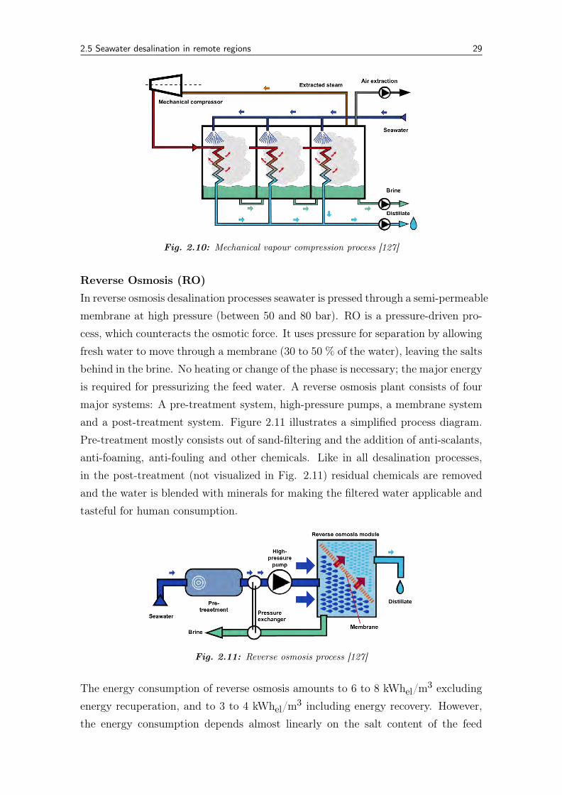
2.5 Seawater desalination in remote regions 29
Fig. 2.10: Mechanical vapour compression process [127]
Reverse Osmosis (RO)
In reverse osmosis desalination processes seawater is pressed through a semi-permeablemembrane at high pressure (between 50 and 80 bar). RO is a pressure-driven pro-cess, which counteracts the osmotic force. It uses pressure for separation by allowingfresh water to move through a membrane (30 to 50 % of the water), leaving the saltsbehind in the brine. No heating or change of the phase is necessary; the major energyis required for pressurizing the feed water. A reverse osmosis plant consists of fourmajor systems: A pre-treatment system, high-pressure pumps, a membrane systemand a post-treatment system. Figure 2.11 illustrates a simplified process diagram.Pre-treatment mostly consists out of sand-filtering and the addition of anti-scalants,anti-foaming, anti-fouling and other chemicals. Like in all desalination processes,in the post-treatment (not visualized in Fig. 2.11) residual chemicals are removedand the water is blended with minerals for making the filtered water applicable andtasteful for human consumption.
Fig. 2.11: Reverse osmosis process [127]
The energy consumption of reverse osmosis amounts to 6 to 8 kWhel/m3 excludingenergy recuperation, and to 3 to 4 kWhel/m3 including energy recovery. However,the energy consumption depends almost linearly on the salt content of the feed
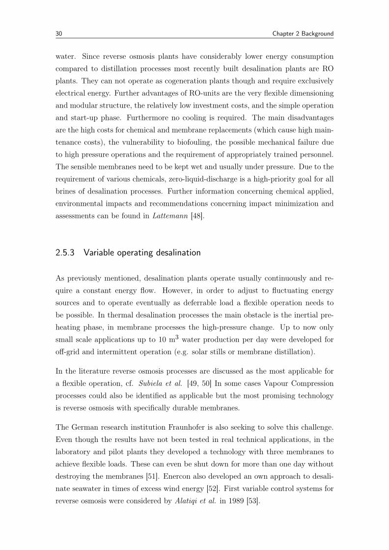
30 Chapter 2 Background
water. Since reverse osmosis plants have considerably lower energy consumptioncompared to distillation processes most recently built desalination plants are ROplants. They can not operate as cogeneration plants though and require exclusivelyelectrical energy. Further advantages of RO-units are the very flexible dimensioningand modular structure, the relatively low investment costs, and the simple operationand start-up phase. Furthermore no cooling is required. The main disadvantagesare the high costs for chemical and membrane replacements (which cause high main-tenance costs), the vulnerability to biofouling, the possible mechanical failure dueto high pressure operations and the requirement of appropriately trained personnel.The sensible membranes need to be kept wet and usually under pressure. Due to therequirement of various chemicals, zero-liquid-discharge is a high-priority goal for allbrines of desalination processes. Further information concerning chemical applied,environmental impacts and recommendations concerning impact minimization andassessments can be found in Lattemann [48].
2.5.3 Variable operating desalination
As previously mentioned, desalination plants operate usually continuously and re-quire a constant energy flow. However, in order to adjust to fluctuating energysources and to operate eventually as deferrable load a flexible operation needs tobe possible. In thermal desalination processes the main obstacle is the inertial pre-heating phase, in membrane processes the high-pressure change. Up to now onlysmall scale applications up to 10 m3 water production per day were developed foroff-grid and intermittent operation (e.g. solar stills or membrane distillation).
In the literature reverse osmosis processes are discussed as the most applicable fora flexible operation, cf. Subiela et al. [49, 50] In some cases Vapour Compressionprocesses could also be identified as applicable but the most promising technologyis reverse osmosis with specifically durable membranes.
The German research institution Fraunhofer is also seeking to solve this challenge.Even though the results have not been tested in real technical applications, in thelaboratory and pilot plants they developed a technology with three membranes toachieve flexible loads. These can even be shut down for more than one day withoutdestroying the membranes [51]. Enercon also developed an own approach to desali-nate seawater in times of excess wind energy [52]. First variable control systems forreverse osmosis were considered by Alatiqi et al. in 1989 [53].
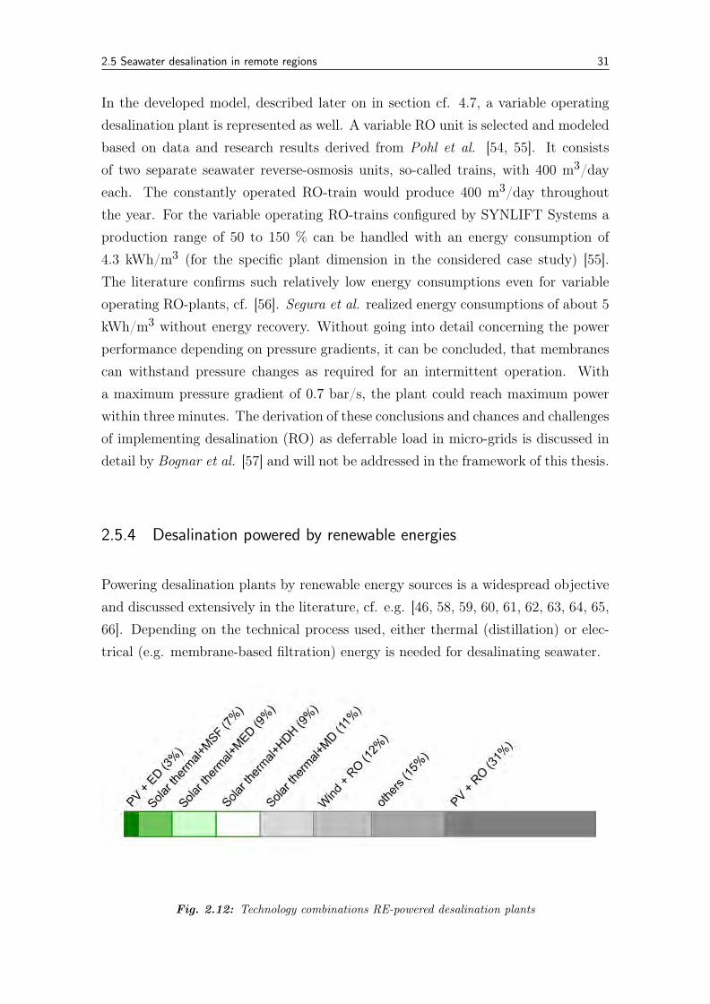
2.5 Seawater desalination in remote regions 31
In the developed model, described later on in section cf. 4.7, a variable operatingdesalination plant is represented as well. A variable RO unit is selected and modeledbased on data and research results derived from Pohl et al. [54, 55]. It consistsof two separate seawater reverse-osmosis units, so-called trains, with 400 m3/dayeach. The constantly operated RO-train would produce 400 m3/day throughoutthe year. For the variable operating RO-trains configured by SYNLIFT Systems aproduction range of 50 to 150 % can be handled with an energy consumption of4.3 kWh/m3 (for the specific plant dimension in the considered case study) [55].The literature confirms such relatively low energy consumptions even for variableoperating RO-plants, cf. [56]. Segura et al. realized energy consumptions of about 5kWh/m3 without energy recovery. Without going into detail concerning the powerperformance depending on pressure gradients, it can be concluded, that membranescan withstand pressure changes as required for an intermittent operation. Witha maximum pressure gradient of 0.7 bar/s, the plant could reach maximum powerwithin three minutes. The derivation of these conclusions and chances and challengesof implementing desalination (RO) as deferrable load in micro-grids is discussed indetail by Bognar et al. [57] and will not be addressed in the framework of this thesis.
2.5.4 Desalination powered by renewable energies
Powering desalination plants by renewable energy sources is a widespread objectiveand discussed extensively in the literature, cf. e.g. [46, 58, 59, 60, 61, 62, 63, 64, 65,66]. Depending on the technical process used, either thermal (distillation) or elec-trical (e.g. membrane-based filtration) energy is needed for desalinating seawater.
Fig. 2.12: Technology combinations RE-powered desalination plants
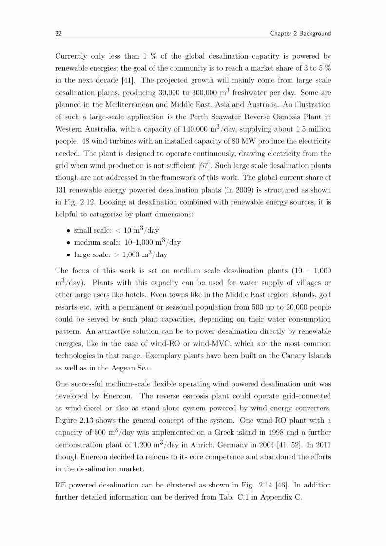
32 Chapter 2 Background
Currently only less than 1 % of the global desalination capacity is powered byrenewable energies; the goal of the community is to reach a market share of 3 to 5 %in the next decade [41]. The projected growth will mainly come from large scaledesalination plants, producing 30,000 to 300,000 m3 freshwater per day. Some areplanned in the Mediterranean and Middle East, Asia and Australia. An illustrationof such a large-scale application is the Perth Seawater Reverse Osmosis Plant inWestern Australia, with a capacity of 140,000 m3/day, supplying about 1.5 millionpeople. 48 wind turbines with an installed capacity of 80 MW produce the electricityneeded. The plant is designed to operate continuously, drawing electricity from thegrid when wind production is not sufficient [67]. Such large scale desalination plantsthough are not addressed in the framework of this work. The global current share of131 renewable energy powered desalination plants (in 2009) is structured as shownin Fig. 2.12. Looking at desalination combined with renewable energy sources, it ishelpful to categorize by plant dimensions:
• small scale: < 10 m3/day• medium scale: 10–1,000 m3/day• large scale: > 1,000 m3/day
The focus of this work is set on medium scale desalination plants (10 – 1,000m3/day). Plants with this capacity can be used for water supply of villages orother large users like hotels. Even towns like in the Middle East region, islands, golfresorts etc. with a permanent or seasonal population from 500 up to 20,000 peoplecould be served by such plant capacities, depending on their water consumptionpattern. An attractive solution can be to power desalination directly by renewableenergies, like in the case of wind-RO or wind-MVC, which are the most commontechnologies in that range. Exemplary plants have been built on the Canary Islandsas well as in the Aegean Sea.
One successful medium-scale flexible operating wind powered desalination unit wasdeveloped by Enercon. The reverse osmosis plant could operate grid-connectedas wind-diesel or also as stand-alone system powered by wind energy converters.Figure 2.13 shows the general concept of the system. One wind-RO plant with acapacity of 500 m3/day was implemented on a Greek island in 1998 and a furtherdemonstration plant of 1,200 m3/day in Aurich, Germany in 2004 [41, 52]. In 2011though Enercon decided to refocus to its core competence and abandoned the effortsin the desalination market.
RE powered desalination can be clustered as shown in Fig. 2.14 [46]. In additionfurther detailed information can be derived from Tab. C.1 in Appendix C.
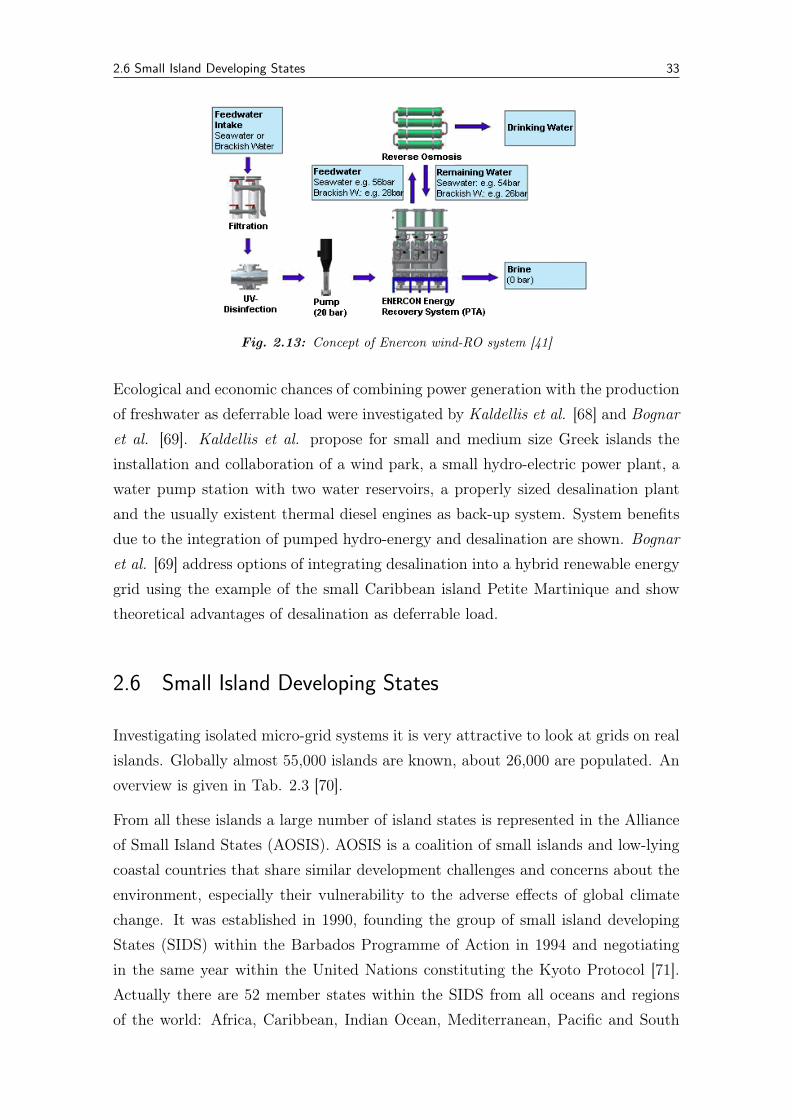
2.6 Small Island Developing States 33
Fig. 2.13: Concept of Enercon wind-RO system [41]
Ecological and economic chances of combining power generation with the productionof freshwater as deferrable load were investigated by Kaldellis et al. [68] and Bognaret al. [69]. Kaldellis et al. propose for small and medium size Greek islands theinstallation and collaboration of a wind park, a small hydro-electric power plant, awater pump station with two water reservoirs, a properly sized desalination plantand the usually existent thermal diesel engines as back-up system. System benefitsdue to the integration of pumped hydro-energy and desalination are shown. Bognaret al. [69] address options of integrating desalination into a hybrid renewable energygrid using the example of the small Caribbean island Petite Martinique and showtheoretical advantages of desalination as deferrable load.
2.6 Small Island Developing States
Investigating isolated micro-grid systems it is very attractive to look at grids on realislands. Globally almost 55,000 islands are known, about 26,000 are populated. Anoverview is given in Tab. 2.3 [70].
From all these islands a large number of island states is represented in the Allianceof Small Island States (AOSIS). AOSIS is a coalition of small islands and low-lyingcoastal countries that share similar development challenges and concerns about theenvironment, especially their vulnerability to the adverse effects of global climatechange. It was established in 1990, founding the group of small island developingStates (SIDS) within the Barbados Programme of Action in 1994 and negotiatingin the same year within the United Nations constituting the Kyoto Protocol [71].Actually there are 52 member states within the SIDS from all oceans and regionsof the world: Africa, Caribbean, Indian Ocean, Mediterranean, Pacific and South
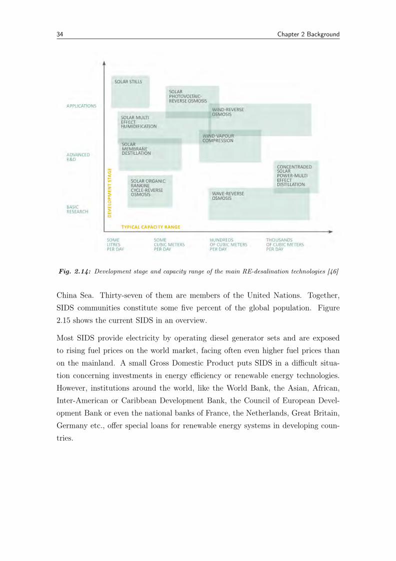
34 Chapter 2 Background
Fig. 2.14: Development stage and capacity range of the main RE-desalination technologies [46]
China Sea. Thirty-seven of them are members of the United Nations. Together,SIDS communities constitute some five percent of the global population. Figure2.15 shows the current SIDS in an overview.
Most SIDS provide electricity by operating diesel generator sets and are exposedto rising fuel prices on the world market, facing often even higher fuel prices thanon the mainland. A small Gross Domestic Product puts SIDS in a difficult situa-tion concerning investments in energy efficiency or renewable energy technologies.However, institutions around the world, like the World Bank, the Asian, African,Inter-American or Caribbean Development Bank, the Council of European Devel-opment Bank or even the national banks of France, the Netherlands, Great Britain,Germany etc., offer special loans for renewable energy systems in developing coun-tries.
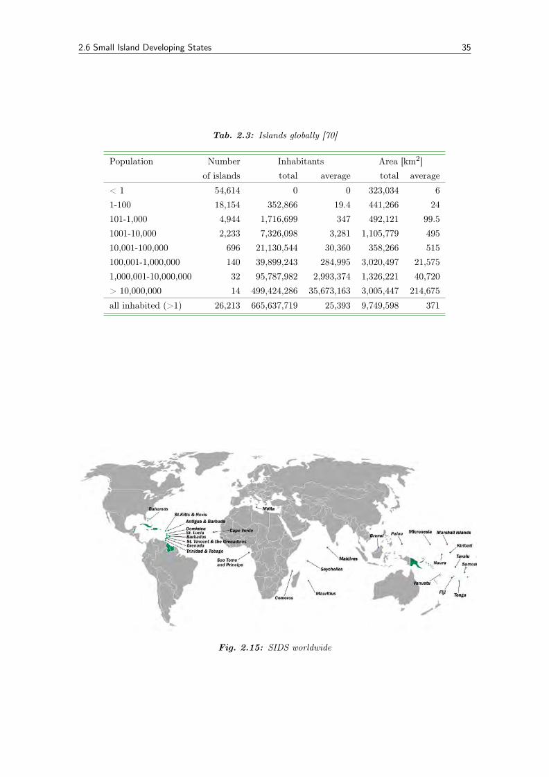
2.6 Small Island Developing States 35
Tab. 2.3: Islands globally [70]
Population Number Inhabitants Area [km2]of islands total average total average
< 1 54,614 0 0 323,034 61-100 18,154 352,866 19.4 441,266 24101-1,000 4,944 1,716,699 347 492,121 99.51001-10,000 2,233 7,326,098 3,281 1,105,779 49510,001-100,000 696 21,130,544 30,360 358,266 515100,001-1,000,000 140 39,899,243 284,995 3,020,497 21,5751,000,001-10,000,000 32 95,787,982 2,993,374 1,326,221 40,720> 10,000,000 14 499,424,286 35,673,163 3,005,447 214,675
all inhabited (>1) 26,213 665,637,719 25,393 9,749,598 371
Fig. 2.15: SIDS worldwide
Chapter
3Methodology
There are various options of simulating and optimizing energy systems and con-cepts. Approaches can be time-step simulations, statistical analysis, mixed-integerprograms for representing inter-temporal restrictions etc. Models principally differin their complexity and level of detail, in the data requirements for generating usefuloutputs, in the availability and reliability of program and their costs. For answeringthe formulated research questions models or one model is required that representsenergy systems as well as desalination concepts and the possibility of integratingdesalination into the simulation and optimization. Before presenting the chosen ap-proach, the most common programs are presented for modeling energy systems aswell as desalination processes.
3.1 Simulation of energy systems
Energy modeling software ranges from only technical models over urban planning toeconomic planning models or combinations of those. From linear to dynamic modelsa wide spectrum of programming is available. Renewable energy concepts are mainlyplanned, developed, and dispatched by supporting tools like INSEL, RETscreen,HYBRID2, HOMER, and other programs. Before presenting the applied modelingapproach, an overview of some available programs is given in Tab. 3.1. Since mostmodels presented in the overview are in continuous development, this list is notexhaustive.
Programs like MARKAL (Market Allocation) are the first linear-programmingmodels for energy-system-analysis minimizing total system costs. MARKAL islodged with GAMS (General Algebraic Modeling System) and was developed within
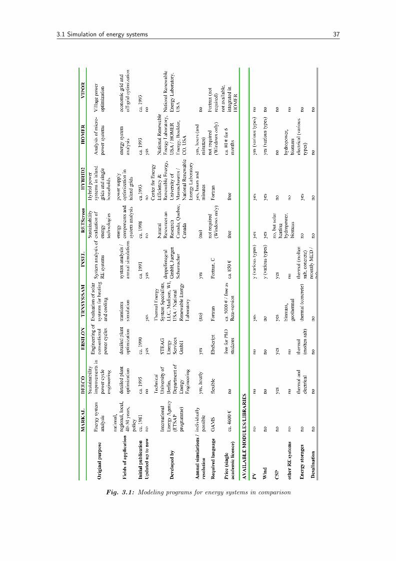
3.1 Simulation of energy systems 37
Fig. 3.1: Modeling programs for energy systems in comparison
38 Chapter 3 Methodology
the Energy Technology Systems Analysis Programme (ETSAP) of the InternationalEnergy Agency, documented by Fishbone and Abilock in 1981 [72]. The main reason,why this model is not used as base was the high price of 6000 USD even for academicpurposes as listed on the MARKAL website. Since significant developments wouldhave been needed anyways, a model development from the scratch was preferred.
Deeco (dynamic energy, emissions, and cost optimization), was developed by Bruck-ner et al. at the Technical University of Berlin. Deeco is an energy system modelingenvironment, which is used to define and evaluate sustainability improvements in-cluding CO2-savings mainly for fossil but also for renewable power plants. Thesoftware requires a high resolution of accurate technical details. The program isnormally used to compute sustainability gains versus costs relative to some assess-ment of business-as-usual by using recursive dynamic optimization techniques, cf.[73]. Since Deeco is optimizing single power plants in a much more detailed approachthan available for most energy systems in remote and developing regions, it is notapplicable for answering the formulated questions.
HOMER is an initially open-source program developed in 1993 by the NationalRenewable Energy Laboratory (NREL) which has been further developed and com-mercialized since then. It is a program which simplifies the task to evaluate differentgrid options no matter whether a grid-connected or off-grid power system is sought.HOMER is capable of modeling a wide range of energy systems including renewableenergy sources (RES) like photovoltaics, wind turbines, hydro power, biogas andconventional systems fired with diesel or gasoline. Furthermore, storage systemslike batteries and hydrogen are supported and can partly be integrated individually.Compared to other simulation tools, HOMER has a very user-friendly interface andhas undergone continuous developments, especially since becoming a commercialproduct (since 2009). In HOMER, the best possible system configuration is theone that satisfies the user-specified constraints at the lowest total net present cost.Finding the optimal system configuration may involve deciding on the mix of com-ponents that the system should contain, the size or quantity of each component, andthe dispatch strategy the system should use [74].
Main disadvantages of each optimization tool are that not all energy conversiontechnologies can be compared and that desalination cannot be integrated the way itwould be required for an overall optimization approach. The best fitting software foranswering the research questions is HOMER, although it is commercial in the mean-time. The license costs are reasonable. A great advantage of HOMER comparedto most other simulation environments is that a deferrable load can be introduced.
3.2 Simulation of desalination units 39
It can only be inserted with characteristics for one day in a month, what is notsufficient for the approached analysis, but still the best for comparing technologieswith each other while considering a shiftable and flexible load within the demandstructure. Initial and some scenario analysis were calculated with HOMER. For fur-ther developments, the integration of desalination processes, and global sensitivityanalysis another model is required though. Applicable models are either too com-plex, working with not accessible algorithms or are too expensive. Developing anown model beginning from scratch seemed to be the best solution.
3.2 Simulation of desalination units
Searching for existent simulation and optimization tools for desalination powered byrenewable energies, one can find around fifteen research programs launched between1998 and 2004, mostly financed by the European Union. Unfortunately only a fewof them were finalized and published. The most relevant ones are listed in Tab. 3.1.
Tab. 3.1: Overview of modeling programs for desalination
Software name Responsible organization and yearof development
Thematic area
SOLDES Abu Dhabi Water and ElectricityAuthority, Saudi Arabia (2000)
solar thermal + MED
REDDES Regional Energy Agency of Do-decanese S.A., Greece, GerlingSustainable Development ProjectGmbh, Germany (2003)
MultiCriteriaAnalysis (MCA) com-bined with GIS-system, RES+DES-potentional
DesalSolar Institut für Verfahrenstechnik,RWTH Aachen, Germany (2002)
solar + desal, small scale < 100m3/day
RESYSproDESAL Center for Solar Energy and Hydro-gen Research, Gerrmany (2006)
stand alone systems, thermal andmembrane processes
ROSA DOW FILMTEC (2011 last version) design software for RO systems (formanufacturers)
SOLDES is a program developed 1998 to 2002 simulating the operation of solardesalination plants, that utilize evacuated tube collectors, heat accumulators andmulti-effect distillation systems. The model is developed and described by El Nashar[75]. Since it focuses on only one specific technology-combination, the model cannotbe used for technology comparisons. The model itself is too detailed for integrating
40 Chapter 3 Methodology
it into the techno-economic model approach, especially because thermal energy anddesalination processes are not the focus of the research approach.
DesalSolar is a computer-based decision support system, useful for selecting thebest desalination and renewable energy technology combination, from the literaturereported combinations, based on site parameters of desalination plant and renewableenergy supply system. Only off-grid stand-alone water and power supply systems areconsidered and their technical and economic performance predicted. The softwareis supervised by the Middle East Desalination Research Center (MEDRC) and canbe accessed from their website.
RESYSproDESAL stands for Renewable Energy SYStems for DESALination. Itis also a software tool for the prediction of the technical and economic performance ofintegrated water and power supply systems using renewable energy and fossil sources.RESYSproDESAL is the most applicable system for selecting feasible renewable en-ergy desalination systems. Small and medium size projects can be designed withspecifically prepared modules for brackish water and seawater. Considered desalina-tion technologies are reverse osmosis, electrodialysis, solar still and humidificationdehumidification. The part of energy conversion is not modeled in detail, only thedesalination part. The license costs for accessing the library and using the full pro-gram would have been too high though. Still, the collaboration with the co-developerJ. Rheinländer, was very helpful.
The modeling approach needed to be adjusted. A new desalination model has beendeveloped in a simplified way, taking into account design layouts, calculated andrecommended by manufacturers. For each desalination technology a cooperationpartner from the industry has been found. Input data and the developed model arebased on information by the manufacturers Terrawater GmbH for HDH [40], Fis-cher eco solutions GmbH for MED [76], Medesa Technology GmbH for MVC [47],and Synlift Systems GmbH for conventional and variable operating RO [55], sup-plemented with further interview partners and data from the technical report of theProDes research program [46]. For determining the optimal conventional and vari-able operating RO-system, the RO design program ROSA has been used. ROSAis provided by the manufacturer DOW FILMTEC and allows system calculationswith its own elements [77]. Based on the expertise of Synlift Systems GmbH, op-timal module parameters have been defined to guarantee a realistic and availablemembrane system. Detailed information concerning the data used within the modelcan be found in section 4.7.
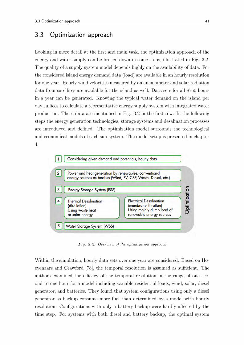
3.3 Optimization approach 41
3.3 Optimization approach
Looking in more detail at the first and main task, the optimization approach of theenergy and water supply can be broken down in some steps, illustrated in Fig. 3.2.The quality of a supply system model depends highly on the availability of data. Forthe considered island energy demand data (load) are available in an hourly resolutionfor one year. Hourly wind velocities measured by an anemometer and solar radiationdata from satellites are available for the island as well. Data sets for all 8760 hoursin a year can be generated. Knowing the typical water demand on the island perday suffices to calculate a representative energy supply system with integrated waterproduction. These data are mentioned in Fig. 3.2 in the first row. In the followingsteps the energy generation technologies, storage systems and desalination processesare introduced and defined. The optimization model surrounds the technologicaland economical models of each sub-system. The model setup is presented in chapter4.
Fig. 3.2: Overview of the optimization approach
Within the simulation, hourly data sets over one year are considered. Based on Ho-evenaars and Crawford [78], the temporal resolution is assumed as sufficient. Theauthors examined the efficacy of the temporal resolution in the range of one sec-ond to one hour for a model including variable residential loads, wind, solar, dieselgenerator, and batteries. They found that system configurations using only a dieselgenerator as backup consume more fuel than determined by a model with hourlyresolution. Configurations with only a battery backup were hardly affected by thetime step. For systems with both diesel and battery backup, the optimal system
42 Chapter 3 Methodology
costs were fairly close in all temporal resolutions but differed in the optimal compo-nent sizes. Since in the given case a diesel generator and batteries are used within allsolutions, a resolution of one hour time steps is assumed to suffice without deformingthe economical optimal results. For exact information about the behaviour of thebattery bank, the fossil and renewable conversion technologies within in each timestep, an analysis with higher temporal resolution would be required. However, be-fore implementing a supply system, an accurate dispatching strategy and frequencystabilization within each hour should be determined. Short-term energy storages aswell as energy control and/or management systems would have to be integrated butare beyond the scope of this study.
3.3.1 GAMS/OSICplex
In order to map al relevant sub-systems in an appropriate model, including avail-able fractions of other modeling approaches and to solve the large scale mathematicaloptimization problem, the programming language GAMS (General Algebraic Mod-eling System) was selected. GAMS does not solve optimization problems directly,but calls appropriate external algorithms. The one used in this work is the IBM’sCplex solver through the GAMS/OSICplex interface. OSICplex is available for freefor six months for academic purposes and is a solver link, that uses the COIN-OROpen Solver Interface (OSI) to communicate with solvers. The OSI links support lin-ear equations and continuous, binary, and integer variables. While semi-continuousand semi-integer variables, special ordered sets, branching priorities, and indicatorconstraints are currently not supported [79], the model presented in this work wascreated taking the mentioned programming limitations into account. Cplex is sup-posed to be the most robust and fastest solver for mixed integer programs usinga number of binary variables. Alternative Solvers with comparable functions areGurobi, distributed by Gurobi Optimization Inc., and ZIMPL, developed by theZuse Institute Berlin.
Through the GAMS/OSICplex interface, a number of parameters were passed tothe solver in order to optimize the use of computational resources and prevent thecomputer form running out of memory. The algorithm used is the primal simplexwith best estimate strategy for node selection and strong branching. As for thecomputer resources management: the time and memory limits are extended fromdefault values; the solver is asked to conserve memory when possible, and it is giventhe possibility to store and compress node files on the disk; advanced basis are used
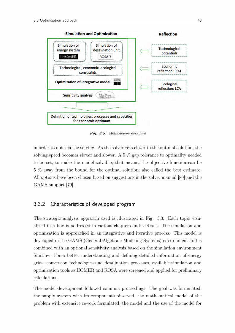
3.3 Optimization approach 43
Fig. 3.3: Methodology overview
in order to quicken the solving. As the solver gets closer to the optimal solution, thesolving speed becomes slower and slower. A 5 % gap tolerance to optimality neededto be set, to make the model solvable; that means, the objective function can be5 % away from the bound for the optimal solution, also called the best estimate.All options have been chosen based on suggestions in the solver manual [80] and theGAMS support [79].
3.3.2 Characteristics of developed program
The strategic analysis approach used is illustrated in Fig. 3.3. Each topic visu-alized in a box is addressed in various chapters and sections. The simulation andoptimization is approached in an integrative and iterative process. This model isdeveloped in the GAMS (General Algebraic Modeling Systems) environment and iscombined with an optional sensitivity analysis based on the simulation environmentSimEnv. For a better understanding and defining detailed information of energygrids, conversion technologies and desalination processes, available simulation andoptimization tools as HOMER and ROSA were screened and applied for preliminarycalculations.
The model development followed common proceedings: The goal was formulated,the supply system with its components observed, the mathematical model of theproblem with extensive rework formulated, the model and the use of the model for
44 Chapter 3 Methodology
prediction verified, suitable alternatives selected if necessary, and recommendationsimplemented, evaluated and reflected. Standard literature used for determining thebasic approach are e.g. [81] and [82]. Typical challenges in modeling and optimizingare minimizing time consumption. Adjustments of the model for minimizing timeconsumption are addressed in each section and at the end of the modeling chapter4.
The model itself is dynamic, because decision variables do involve sequences of de-cisions over multiple periods. During the construction of the model a particularattention was paid to keep the model linear. While non-linear models enable theimplementation to have more sophisticated dependencies between variables, thusallowing more complicated sub-models, this model was kept intentionally linear toenhance its speed and its convergence in respect to initial values. A non-linear pro-gram with the dimension of 8760 time steps, various energy generation technologiesand storage systems, would not be solvable. Sub-models that may have requirednon-linear structures were linearized through reasonable assumptions or turned intomodels with piecewise linear dependencies. Because most energy generation, storageand desalination units need to be switched on an off during the operation within oneyear, the integration of binary variables, responsible for switching technologies onand off, is essential. Linear programs turn into mixed integer programs. A furthercharacteristic of a model is the question, whether it is deterministic or stochastic.Although there are a number of uncertain values, as the oil price, wind and solarpotentials or demand developments, the model is designed as deterministic model.
The Mixed Integer Programming (MIP) algorithm used is an implementation of abranch-and-bound search with specific algorithmic features such as cuts and heuris-tics. The branch-and-bound algorithm discards a significant part of unused sub-systems by using upper and lower estimated bounds. The method was first proposedin 1960 for discrete programming [83]. Lagrange-multiplier can also be introduced ifrequired. The MIP optimizer within OSICplex solves large and numerically difficultMIP models [80]. Integer variables, different branchings and nodes have been de-fined. As mentioned before, OSICplex faces limitations compared to Cplex. One, forexample, is the fact, that in comparison to Cplex OSICplex does not support specialorder sets (SOS) of order 1 and 2. That means, parameters with one or two positivevariables are provided with a set of specific conditions and boundaries, in case oftwo positive variables (SOS2), the variables need to be adjacent and the adjacencyconditions are enforced by the solution algorithm. Most commercial solvers allowto specify SOS1 and SOS2, OSICplex not. Therefore alternatives need to be formu-
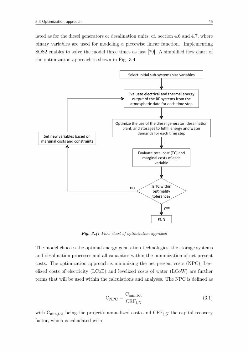
3.3 Optimization approach 45
lated as for the diesel generators or desalination units, cf. section 4.6 and 4.7, wherebinary variables are used for modeling a piecewise linear function. ImplementingSOS2 enables to solve the model three times as fast [79]. A simplified flow chart ofthe optimization approach is shown in Fig. 3.4.
Fig. 3.4: Flow chart of optimization approach
The model chooses the optimal energy generation technologies, the storage systemsand desalination processes and all capacities within the minimization of net presentcosts. The optimization approach is minimizing the net present costs (NPC). Lev-elized costs of electricity (LCoE) and levelized costs of water (LCoW) are furtherterms that will be used within the calculations and analyses. The NPC is defined as
CNPC =Cann,totCRFi,N
(3.1)
with Cann,tot being the project’s annualized costs and CRFi,N the capital recoveryfactor, which is calculated with
46 Chapter 3 Methodology
CRFir,N =ir(1 + ir)N
(1 + ir)N – 1(3.2)
whereas ir stands for the annual real interest rate and N for the projects lifetime.The inflation adjusted real interest rate is defined as
ir = in – j (3.3)
with ir labeling the real interest rate, in the nominal interest rate and j the inflationrate.
The levelized costs of energy (LCoE) are calculated as shown in Eq. 3.4, the levelizedcosts of water (LCoW) according to Eq. 3.5. Both equations use the annuity factor(Ai,N), where i is equal to 0.075 and N to 20 years (cf. Eq. 3.6).
LCoE =I0E · Ai,N + Cfuel + CO&ME
Eprim(3.4)
LCoW =I0W · Ai,N + CO&MW + CE
Wyear(3.5)
Ai,N =i · (1 + i)N
(1 + i)N – 1(3.6)
In Eq. 3.4 the initial capital costs (I0E) multiplied by the annuity factor reflect theannual capital expenditures. CO&ME stands for operation and maintenance costs ofall components per year, and Cfuel stands for annual fuel costs. All annual costs aredivided by the primary load (Eprim). The additional energy demand for desalinationis not added to the primary load in order to keep the scenarios comparable withoutminimizing the LCoE due to the increased electricity demand. To calculate theLCoW, the initial capital cost of the desalination plant I0W multiplied by the annuityfactor is added to the annual costs of the desalination plant, including operation andmaintenance costs (CO&MW) and electricity costs (CE). These are divided by theamount of potable water produced in the year (Wyear).
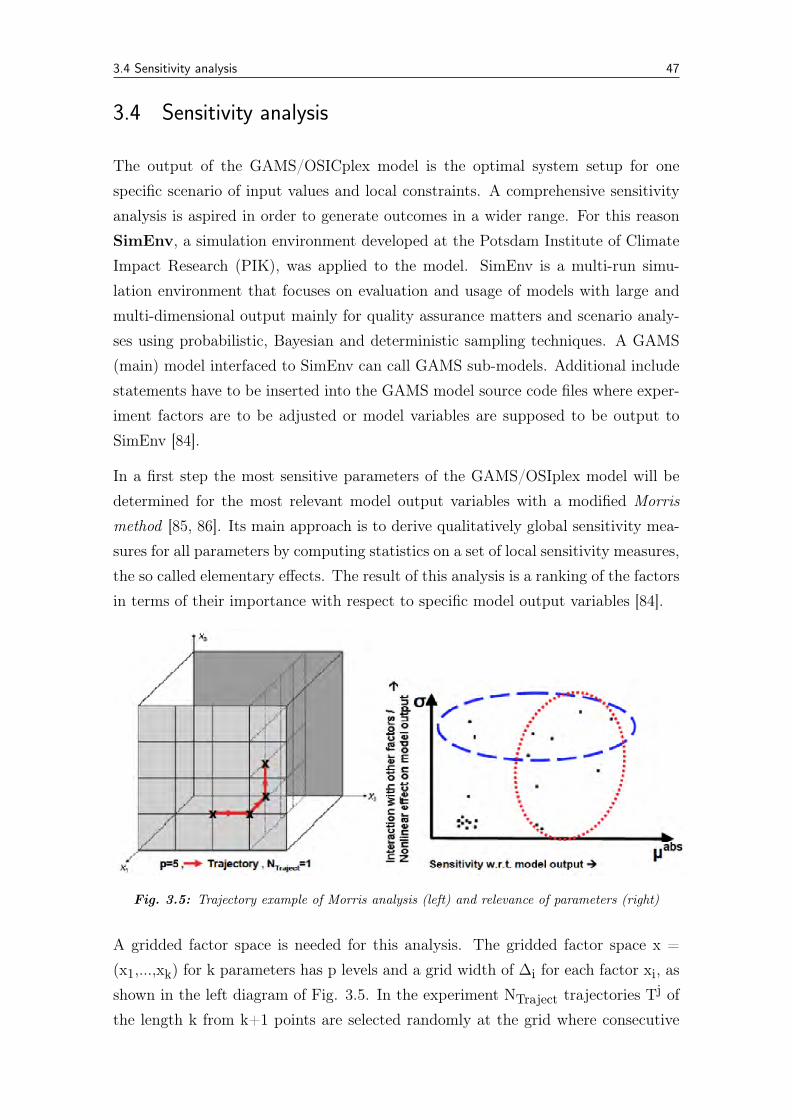
3.4 Sensitivity analysis 47
3.4 Sensitivity analysis
The output of the GAMS/OSICplex model is the optimal system setup for onespecific scenario of input values and local constraints. A comprehensive sensitivityanalysis is aspired in order to generate outcomes in a wider range. For this reasonSimEnv, a simulation environment developed at the Potsdam Institute of ClimateImpact Research (PIK), was applied to the model. SimEnv is a multi-run simu-lation environment that focuses on evaluation and usage of models with large andmulti-dimensional output mainly for quality assurance matters and scenario analy-ses using probabilistic, Bayesian and deterministic sampling techniques. A GAMS(main) model interfaced to SimEnv can call GAMS sub-models. Additional includestatements have to be inserted into the GAMS model source code files where exper-iment factors are to be adjusted or model variables are supposed to be output toSimEnv [84].
In a first step the most sensitive parameters of the GAMS/OSIplex model will bedetermined for the most relevant model output variables with a modified Morrismethod [85, 86]. Its main approach is to derive qualitatively global sensitivity mea-sures for all parameters by computing statistics on a set of local sensitivity measures,the so called elementary effects. The result of this analysis is a ranking of the factorsin terms of their importance with respect to specific model output variables [84].
Fig. 3.5: Trajectory example of Morris analysis (left) and relevance of parameters (right)
A gridded factor space is needed for this analysis. The gridded factor space x =(x1,...,xk) for k parameters has p levels and a grid width of Δi for each factor xi, asshown in the left diagram of Fig. 3.5. In the experiment NTraject trajectories Tj ofthe length k from k+1 points are selected randomly at the grid where consecutive
48 Chapter 3 Methodology
points differ only in one factor. For each trajectory Tj=(t1j ,.., tk+1j) and each
factor xi from two consecutive points an elementary effect eeij = (y(tlj+ei Δi) -y(tl+1
j)) / Δi is determined. The arrows in the left coordinate system of Fig. 3.5indicate the sequence how each trajectory is generated from sampling points [84].In a next step distribution measures from the eeij are determined (refer to [84] forfurther details) and are characterized by the sensitivity μi and variance σi. μi inthis case stands for the overall influence of xi on y, that means for the sensitivityof a factor with respect to the model output. σi shows, whether the factor xi isinvolved in interactions with other factors with respect to y or if the effect of xi ony is nonlinear. The right diagram of Fig. 3.5 gives an idea of how such a qualitativeinterpretation of sensitive parameters based on a number of elementary effects canbe visualized for one model output y. Factors within the red circle can be identifiedas most sensitive, factors bounded by the blue circle show interactions with otherfactors and/or a nonlinear effect on the model output y. Parameters can be rankednow with respect to their sensitivity. The computational cost C in terms of thenumber of single model runs of such an experiment is C = NTraject · (k + 1) [84].
After determining the most sensitive parameters and variables, a sensitivity anal-ysis is performed based on these sensitive parameters by choosing a DeterministicFactorial Design. Without going into more detail, the goal of this approach is toshow how the model behaviour changes with deterministic changes of factor values,cf. [84] for further information.
For deriving statistical conclusions concerning the distribution of energy mixes andbeneficial technology combinations, a Monte-Carlo-Analysis is undertaken for themost sensitive parameters as well. The resulting probability density function ofmodel output y can also be interpreted as a stochastic error analysis, but is used heremore for determining the relevance from different energy generation and desalinationcomponents. The detailed proceeding is documented in combination with the resultsin section 6.5.
3.5 Real option analysis
Traditionally the cost-benefit analysis [87], the net present value and the discountedcash flow methods are used to evaluate project investments. As soft evaluationmethods the cost-utility analysis and the multi-criteria analysis are most commonlyused. In the developed model the net present cost approach is employed.
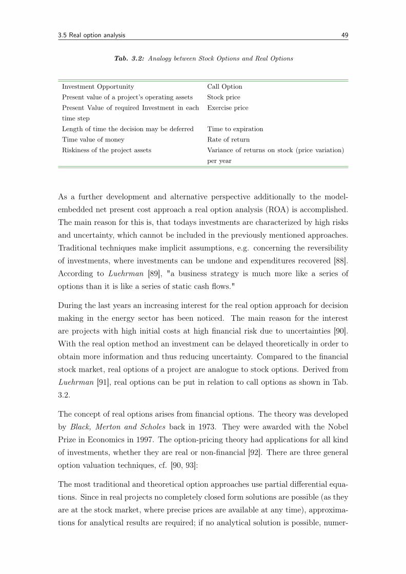
3.5 Real option analysis 49
Tab. 3.2: Analogy between Stock Options and Real Options
Investment Opportunity Call OptionPresent value of a project’s operating assets Stock pricePresent Value of required Investment in eachtime step
Exercise price
Length of time the decision may be deferred Time to expirationTime value of money Rate of returnRiskiness of the project assets Variance of returns on stock (price variation)
per year
As a further development and alternative perspective additionally to the model-embedded net present cost approach a real option analysis (ROA) is accomplished.The main reason for this is, that todays investments are characterized by high risksand uncertainty, which cannot be included in the previously mentioned approaches.Traditional techniques make implicit assumptions, e.g. concerning the reversibilityof investments, where investments can be undone and expenditures recovered [88].According to Luehrman [89], "a business strategy is much more like a series ofoptions than it is like a series of static cash flows."
During the last years an increasing interest for the real option approach for decisionmaking in the energy sector has been noticed. The main reason for the interestare projects with high initial costs at high financial risk due to uncertainties [90].With the real option method an investment can be delayed theoretically in order toobtain more information and thus reducing uncertainty. Compared to the financialstock market, real options of a project are analogue to stock options. Derived fromLuehrman [91], real options can be put in relation to call options as shown in Tab.3.2.
The concept of real options arises from financial options. The theory was developedby Black, Merton and Scholes back in 1973. They were awarded with the NobelPrize in Economics in 1997. The option-pricing theory had applications for all kindof investments, whether they are real or non-financial [92]. There are three generaloption valuation techniques, cf. [90, 93]:
The most traditional and theoretical option approaches use partial differential equa-tions. Since in real projects no completely closed form solutions are possible (as theyare at the stock market, where precise prices are available at any time), approxima-tions for analytical results are required; if no analytical solution is possible, numer-
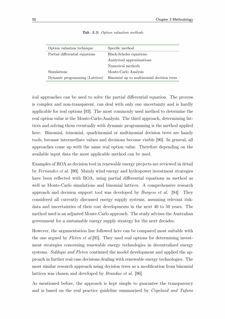
50 Chapter 3 Methodology
Tab. 3.3: Option valuation methods
Option valuation technique Specific method
Partial differential equations Black-Scholes equationsAnalytical approximationsNumerical methods
Simulations Monte-Carlo AnalysisDynamic programming (Lattices) Binomial up to multinomial decision trees
ical approaches can be used to solve the partial differential equation. The processis complex and non-transparent, can deal with only one uncertainty and is hardlyapplicable for real options [93]. The most commonly used method to determine thereal option value is the Monte-Carlo-Analysis. The third approach, determining lat-tices and solving them eventually with dynamic programming is the method appliedhere. Binomial, trinomial, quadrinomial or multinomial decision trees are handytools, because intermediate values and decisions become visible [90]. In general, allapproaches come up with the same real option value. Therefore depending on theavailable input data the most applicable method can be used.
Examples of ROA as decision tool in renewable energy projects are reviewed in detailby Fernandes et al. [90]. Mainly wind energy and hydropower investment strategieshave been reflected with ROA, using partial differential equations as method aswell as Monte-Carlo simulations and binomial lattices. A comprehensive researchapproach and decision support tool was developed by Burgess et al. [94]. Theyconsidered all currently discussed energy supply systems, assuming relevant risk-data and uncertainties of their cost developments in the next 40 to 50 years. Themethod used is an adjusted Monte-Carlo approach. The study advises the Australiangovernment for a sustainable energy supply strategy for the next decades.
However, the argumentation line followed here can be compared most suitable withthe one argued by Fleten et al.[95]. They used real options for determining invest-ment strategies concerning renewable energy technologies in decentralized energysystems. Siddiqui and Fleten continued the model development and applied the ap-proach in further real case decisions dealing with renewable energy technologies. Themost similar research approach using decision trees as a modification from binomiallattices was chosen and developed by Brandao et al. [96].
As mentioned before, the approach is kept simple to guarantee the transparencyand is based on the real practice guideline summarized by Copeland and Tufano
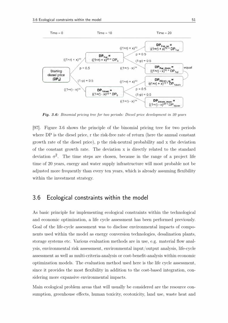
3.6 Ecological constraints within the model 51
Fig. 3.6: Binomial pricing tree for two periods: Diesel price development in 20 years
[97]. Figure 3.6 shows the principle of the binomial pricing tree for two periodswhere DP is the diesel price, r the risk-free rate of return (here the annual constantgrowth rate of the diesel price), p the risk-neutral probability and x the deviationof the constant growth rate. The deviation x is directly related to the standarddeviation σ2. The time steps are chosen, because in the range of a project lifetime of 20 years, energy and water supply infrastructure will most probable not beadjusted more frequently than every ten years, which is already assuming flexibilitywithin the investment strategy.
3.6 Ecological constraints within the model
As basic principle for implementing ecological constraints within the technologicaland economic optimization, a life cycle assessment has been performed previously.Goal of the life-cycle assessment was to disclose environmental impacts of compo-nents used within the model as energy conversion technologies, desalination plants,storage systems etc. Various evaluation methods are in use, e.g. material flow anal-ysis, environmental risk assessment, environmental input/output analysis, life-cycleassessment as well as multi-criteria-analysis or cost-benefit-analysis within economicoptimization models. The evaluation method used here is the life cycle assessment,since it provides the most flexibility in addition to the cost-based integration, con-sidering more expansive environmental impacts.
Main ecological problem areas that will usually be considered are the resource con-sumption, greenhouse effects, human toxicity, ecotoxicity, land use, waste heat and
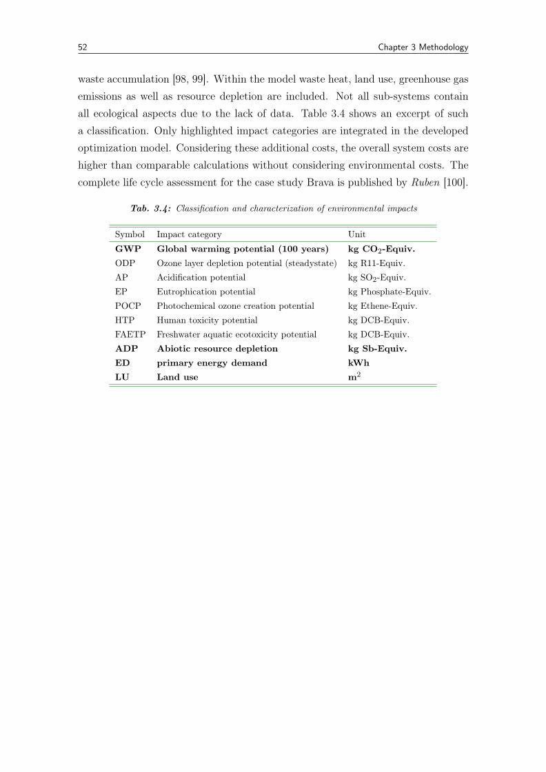
52 Chapter 3 Methodology
waste accumulation [98, 99]. Within the model waste heat, land use, greenhouse gasemissions as well as resource depletion are included. Not all sub-systems containall ecological aspects due to the lack of data. Table 3.4 shows an excerpt of sucha classification. Only highlighted impact categories are integrated in the developedoptimization model. Considering these additional costs, the overall system costs arehigher than comparable calculations without considering environmental costs. Thecomplete life cycle assessment for the case study Brava is published by Ruben [100].
Tab. 3.4: Classification and characterization of environmental impacts
Symbol Impact category Unit
GWP Global warming potential (100 years) kg CO2-Equiv.ODP Ozone layer depletion potential (steadystate) kg R11-Equiv.AP Acidification potential kg SO2-Equiv.EP Eutrophication potential kg Phosphate-Equiv.POCP Photochemical ozone creation potential kg Ethene-Equiv.HTP Human toxicity potential kg DCB-Equiv.FAETP Freshwater aquatic ecotoxicity potential kg DCB-Equiv.ADP Abiotic resource depletion kg Sb-Equiv.ED primary energy demand kWhLU Land use m2
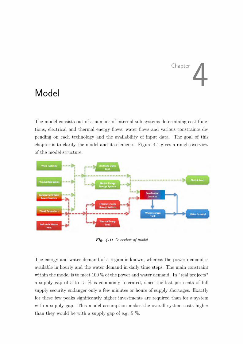
Chapter
4Model
The model consists out of a number of internal sub-systems determining cost func-tions, electrical and thermal energy flows, water flows and various constraints de-pending on each technology and the availability of input data. The goal of thischapter is to clarify the model and its elements. Figure 4.1 gives a rough overviewof the model structure.
Fig. 4.1: Overview of model
The energy and water demand of a region is known, whereas the power demand isavailable in hourly and the water demand in daily time steps. The main constraintwithin the model is to meet 100 % of the power and water demand. In "real projects"a supply gap of 5 to 15 % is commonly tolerated, since the last per cents of fullsupply security endanger only a few minutes or hours of supply shortages. Exactlyfor these few peaks significantly higher investments are required than for a systemwith a supply gap. This model assumption makes the overall system costs higherthan they would be with a supply gap of e.g. 5 %.
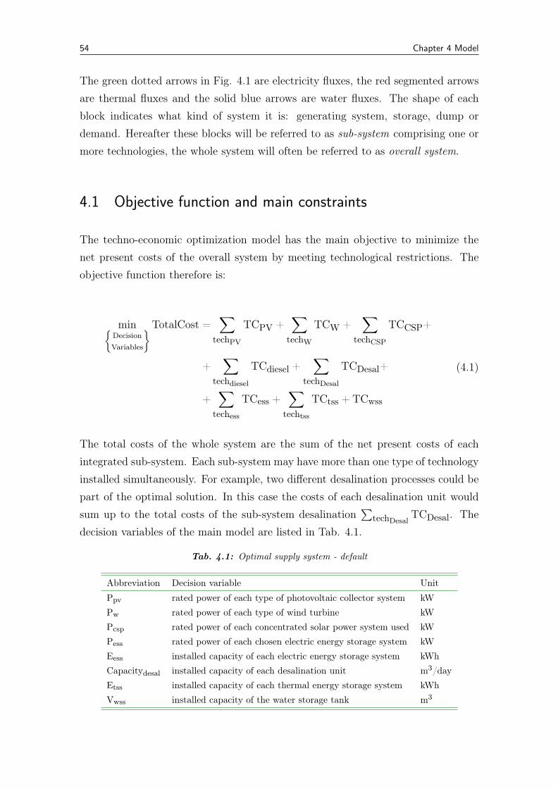
54 Chapter 4 Model
The green dotted arrows in Fig. 4.1 are electricity fluxes, the red segmented arrowsare thermal fluxes and the solid blue arrows are water fluxes. The shape of eachblock indicates what kind of system it is: generating system, storage, dump ordemand. Hereafter these blocks will be referred to as sub-system comprising one ormore technologies, the whole system will often be referred to as overall system.
4.1 Objective function and main constraints
The techno-economic optimization model has the main objective to minimize thenet present costs of the overall system by meeting technological restrictions. Theobjective function therefore is:
min{DecisionVariables
}TotalCost =∑
techPV
TCPV +∑
techW
TCW +∑
techCSP
TCCSP+
+∑
techdiesel
TCdiesel +∑
techDesal
TCDesal+
+∑
techess
TCess +∑
techtss
TCtss + TCwss
(4.1)
The total costs of the whole system are the sum of the net present costs of eachintegrated sub-system. Each sub-system may have more than one type of technologyinstalled simultaneously. For example, two different desalination processes could bepart of the optimal solution. In this case the costs of each desalination unit wouldsum up to the total costs of the sub-system desalination
∑techDesal
TCDesal. Thedecision variables of the main model are listed in Tab. 4.1.
Tab. 4.1: Optimal supply system - default
Abbreviation Decision variable Unit
Ppv rated power of each type of photovoltaic collector system kWPw rated power of each type of wind turbine kWPcsp rated power of each concentrated solar power system used kWPess rated power of each chosen electric energy storage system kWEess installed capacity of each electric energy storage system kWhCapacitydesal installed capacity of each desalination unit m3/dayEtss installed capacity of each thermal energy storage system kWhVwss installed capacity of the water storage tank m3
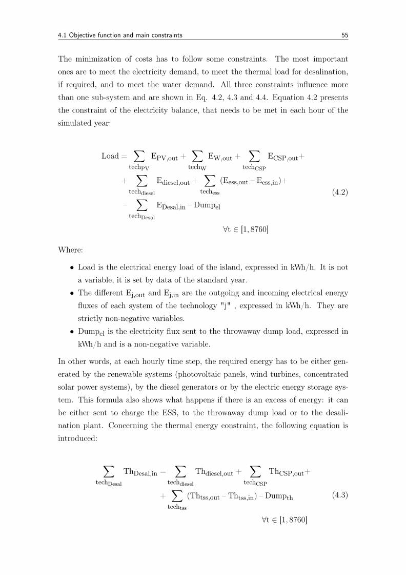
4.1 Objective function and main constraints 55
The minimization of costs has to follow some constraints. The most importantones are to meet the electricity demand, to meet the thermal load for desalination,if required, and to meet the water demand. All three constraints influence morethan one sub-system and are shown in Eq. 4.2, 4.3 and 4.4. Equation 4.2 presentsthe constraint of the electricity balance, that needs to be met in each hour of thesimulated year:
Load =∑
techPV
EPV,out +∑
techW
EW,out +∑
techCSP
ECSP,out+
+∑
techdiesel
Ediesel,out +∑
techess
(Eess,out – Eess,in)+
–∑
techDesal
EDesal,in – Dumpel
∀t ∈ [1, 8760]
(4.2)
Where:
• Load is the electrical energy load of the island, expressed in kWh/h. It is nota variable, it is set by data of the standard year.• The different Ej,out and Ej,in are the outgoing and incoming electrical energy
fluxes of each system of the technology "j" , expressed in kWh/h. They arestrictly non-negative variables.• Dumpel is the electricity flux sent to the throwaway dump load, expressed in
kWh/h and is a non-negative variable.
In other words, at each hourly time step, the required energy has to be either gen-erated by the renewable systems (photovoltaic panels, wind turbines, concentratedsolar power systems), by the diesel generators or by the electric energy storage sys-tem. This formula also shows what happens if there is an excess of energy: it canbe either sent to charge the ESS, to the throwaway dump load or to the desali-nation plant. Concerning the thermal energy constraint, the following equation isintroduced:
∑techDesal
ThDesal,in =∑
techdiesel
Thdiesel,out +∑
techCSP
ThCSP,out+
+∑
techtss
(Thtss,out – Thtss,in) – Dumpth
∀t ∈ [1, 8760]
(4.3)
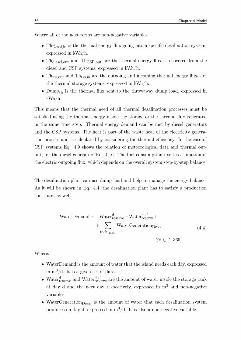
56 Chapter 4 Model
Where all of the next terms are non-negative variables:
• ThDesal,in is the thermal energy flux going into a specific desalination system,expressed in kWh/h.• Thdiesel,out and ThCSP,out are the thermal energy fluxes recovered from the
diesel and CSP systems, expressed in kWh/h.• Thtss,out and Thtss,in are the outgoing and incoming thermal energy fluxes of
the thermal storage systems, expressed in kWh/h.• Dumpth is the thermal flux sent to the throwaway dump load, expressed in
kWh/h.
This means that the thermal need of all thermal desalination processes must besatisfied using the thermal energy inside the storage or the thermal flux generatedin the same time step. Thermal energy demand can be met by diesel generatorsand the CSP systems. The heat is part of the waste heat of the electricity genera-tion process and is calculated by considering the thermal efficiency. In the case ofCSP systems Eq. 4.9 shows the relation of meteorological data and thermal out-put, for the diesel generators Eq. 4.16. The fuel consumption itself is a function ofthe electric outgoing flux, which depends on the overall system step-by-step balance.
The desalination plant can use dump load and help to manage the energy balance.As it will be shown in Eq. 4.4, the desalination plant has to satisfy a productionconstraint as well.
WaterDemand = Waterdreserve – Waterd+1reserve+
+∑
techDesal
WaterGenerationDesal
∀d ∈ [1, 365]
(4.4)
Where:
• WaterDemand is the amount of water that the island needs each day, expressedin m3/d. It is a given set of data.• Waterdreserve and Waterd+1
reserve are the amount of water inside the storage tankat day d and the next day respectively, expressed in m3 and non-negativevariables.• WaterGenerationDesal is the amount of water that each desalination system
produces on day d, expressed in m3/d. It is also a non-negative variable.
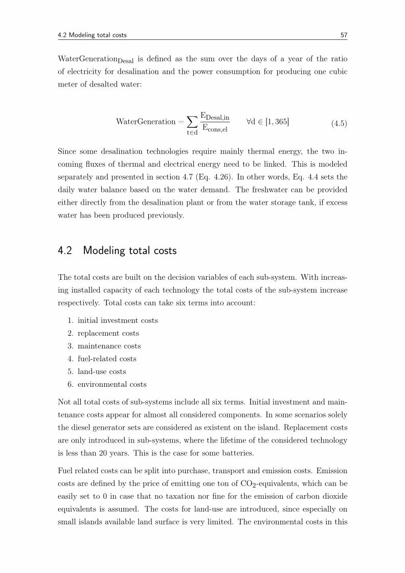
4.2 Modeling total costs 57
WaterGenerationDesal is defined as the sum over the days of a year of the ratioof electricity for desalination and the power consumption for producing one cubicmeter of desalted water:
WaterGeneration =∑t∈d
EDesal,inEcons,el
∀d ∈ [1, 365] (4.5)
Since some desalination technologies require mainly thermal energy, the two in-coming fluxes of thermal and electrical energy need to be linked. This is modeledseparately and presented in section 4.7 (Eq. 4.26). In other words, Eq. 4.4 sets thedaily water balance based on the water demand. The freshwater can be providedeither directly from the desalination plant or from the water storage tank, if excesswater has been produced previously.
4.2 Modeling total costs
The total costs are built on the decision variables of each sub-system. With increas-ing installed capacity of each technology the total costs of the sub-system increaserespectively. Total costs can take six terms into account:
1. initial investment costs2. replacement costs3. maintenance costs4. fuel-related costs5. land-use costs6. environmental costs
Not all total costs of sub-systems include all six terms. Initial investment and main-tenance costs appear for almost all considered components. In some scenarios solelythe diesel generator sets are considered as existent on the island. Replacement costsare only introduced in sub-systems, where the lifetime of the considered technologyis less than 20 years. This is the case for some batteries.
Fuel related costs can be split into purchase, transport and emission costs. Emissioncosts are defined by the price of emitting one ton of CO2-equivalents, which can beeasily set to 0 in case that no taxation nor fine for the emission of carbon dioxideequivalents is assumed. The costs for land-use are introduced, since especially onsmall islands available land surface is very limited. The environmental costs in this
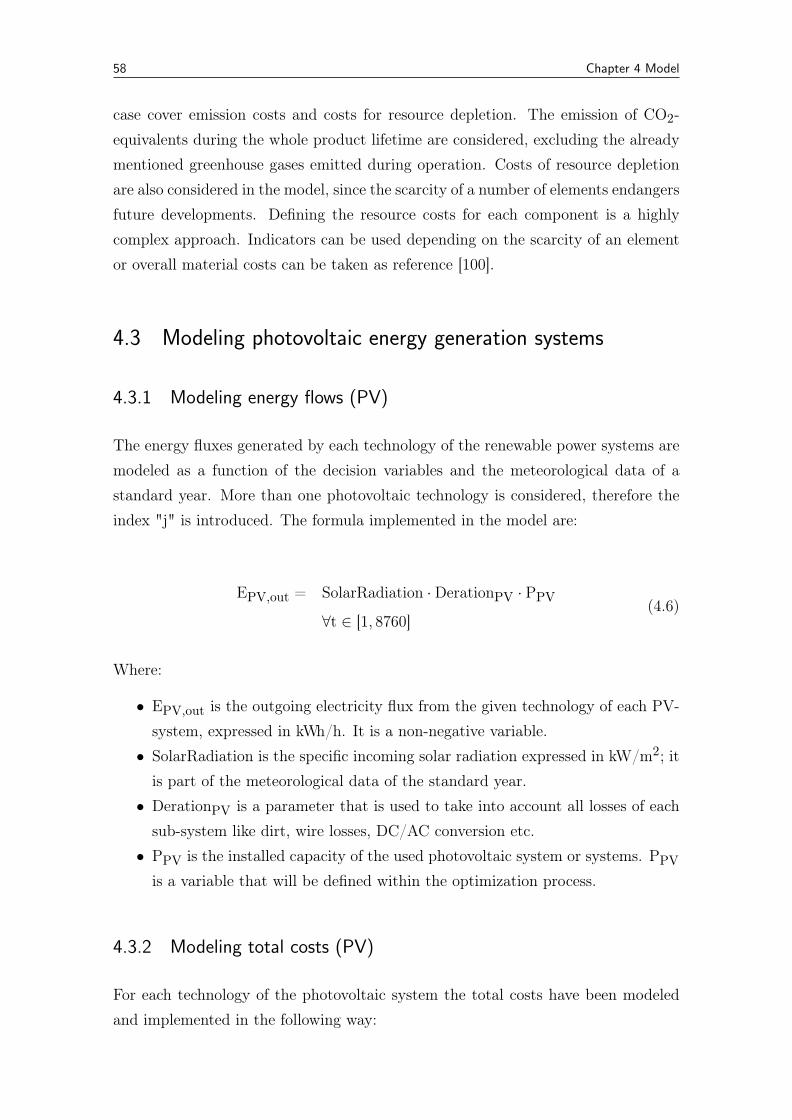
58 Chapter 4 Model
case cover emission costs and costs for resource depletion. The emission of CO2-equivalents during the whole product lifetime are considered, excluding the alreadymentioned greenhouse gases emitted during operation. Costs of resource depletionare also considered in the model, since the scarcity of a number of elements endangersfuture developments. Defining the resource costs for each component is a highlycomplex approach. Indicators can be used depending on the scarcity of an elementor overall material costs can be taken as reference [100].
4.3 Modeling photovoltaic energy generation systems
4.3.1 Modeling energy flows (PV)
The energy fluxes generated by each technology of the renewable power systems aremodeled as a function of the decision variables and the meteorological data of astandard year. More than one photovoltaic technology is considered, therefore theindex "j" is introduced. The formula implemented in the model are:
EPV,out = SolarRadiation ·DerationPV · PPV
∀t ∈ [1, 8760](4.6)
Where:
• EPV,out is the outgoing electricity flux from the given technology of each PV-system, expressed in kWh/h. It is a non-negative variable.• SolarRadiation is the specific incoming solar radiation expressed in kW/m2; it
is part of the meteorological data of the standard year.• DerationPV is a parameter that is used to take into account all losses of each
sub-system like dirt, wire losses, DC/AC conversion etc.• PPV is the installed capacity of the used photovoltaic system or systems. PPV
is a variable that will be defined within the optimization process.
4.3.2 Modeling total costs (PV)
For each technology of the photovoltaic system the total costs have been modeledand implemented in the following way:
4.4 Modeling concentrated solar power systems 59
TCPV = cPPPV
(1 + fO&M
Life∑y=1
1(1 + i)y
)+
+cland
(PPVη· kLU
)+ PPV
(cPV,CO2 + cPV,Res
) (4.7)
The investment cost is modeled as the specific power cost (cP in e/kW) times thepeak installed power of the given technology. The annual operation and maintenancecosts are included as a percentage (fO&M in y–1) of the investment cost and areactualized by the actualization factor. The cost for land use is implemented as thespecific mean land cost (cland in e/m2) on the island times the area occupied bythe system.
The net collecting area of the panels is calculated by the division of the rated powerby the conversion efficiency. The coefficient kLU takes into account the area neededfor the construction, the space between the modules and all equipment required foroperating and managing the system. This coefficient has been set to 1.5. It has beenassumed that the land area required for the system is 50% more then the collector’snet surface. The environmental costs cPV,CO2 and cPV,Res are depending on theinstalled capacity of the PV system and are put together out of the specific lifetime-emission costs and the resource costs.Replacement costs and fuel-related costs can be neglected for PV systems.
4.4 Modeling concentrated solar power systems
4.4.1 Modeling energy flows (CSP)
ECSP,out = SolarRadiation ·DerationCSP · PCSP
∀t ∈ [1, 8760](4.8)
ThCSP,out = SolarRadiation ·DerationCSP · PCSP ·ηCSP,thηCSP,el
∀t ∈ [1, 8760](4.9)
Where:
• SolarRadiation is the specific solar radiation expressed in kW/m2; it is part ofthe meteorological data of the standard year.
60 Chapter 4 Model
• DerationCSP is a parameter, that incloses all losses during energy conversionby the CSP technologies, e.g. due to dirt, wire losses, or general conversionlosses.• ηCSP,el is the electrical efficiency of each CSP technology• ηCSP,th is the thermal efficiency of each CSP technology; it represents the
recovered waste heat divided by the solar radiation. This way, the ratio ηCSP,thηCSP,el
is the amount of thermal energy recovered by generating one unit of electricalenergy.• ECSP,out is the outgoing electricity flux of each CSP technology, expressed in
kWh/h. It is a non-negative variable.• ThCSP,out is the outgoing thermal energy flux of each CSP technology, ex-
pressed in kWh/h. It is also a non-negative variable.
4.4.2 Modeling total costs (CSP)
The total cost of each CSP technology is modeled similar to the PV system:
TCCSP = cPPCSP +(cP,O&MPCSP
Life∑y=1
1(1 + i)y
)+
+cland(LUCSPPCSP) + PCSP
(cCSP,CO2 + cCSP,Res
) (4.10)
The investment cost is modeled identical to the PV systems, the operation andmaintenance cost though is given as a specific cost (cP,O&M in e/kW y) and notas a percentage of the investment cost. The reason for this is solely the availabilityof data. If needed, the formula can be rewritten as percentage, using the formulafO&M = cO&M/cP. The costs for land use are not calculated by a factor but bya specific parameter (LU in m2/kW), multiplying the specific mean land cost bythe required area. The environmental costs for emissions and resource depletion aredetermined as mentioned before for the PV systems.
4.5 Modeling wind energy generation systems
4.5.1 Modeling energy flows (wind)
As wind energy converters three technologies are considered, two with a horizontalaxis, one with a vertical one. For all following energy flow formula is valid:
4.5 Modeling wind energy generation systems 61
EW,out = SpecificOutput(WindSpeed) · PWPW,nom
∀t ∈ [1, 8760](4.11)
Where:
• SpecificOutput(WindSpeed) is the specific electrical energy output of the stan-dard wind turbine. It is a parameter depending on the wind velocity each hour,modeled with a 6th order polynomial curve that fits the power-windspeed curvegiven by manufacturers and expressed in kWh/h. Details are discussed below.• PW,nom is the nominal power of the considered wind turbine. The ratio of PW
serves as a scaling factor under the assumption that the power-wind speedcurve grows and is reduced proportionally with the rated power, maintainingthe same shape.• EW,out is the outgoing electricity flux of each wind technology, expressed in
kWh/h. It is a non-negative variable.
The wind speed is part of the meteorological data and is given at the height of themeasuring anemometer. To evaluate the velocity at hub height, which can changebetween different types of wind turbines, the following formula is used:
VHubHeight = Vanemometer
(ln(hhub/z0)
ln(hanemometer/z0)
)∀t ∈ [1, 8760] (4.12)
Where z0 is the roughness of the ground around the wind turbine and h is the height.Both are expressed in meters.
The specific output of a wind turbine depends on its power curve. The model isa linear mixed integer program. The non-linear power curve of a wind turbine canbe approximated by a polynomial and some further parameters. The power curveof the wind turbines can be fit the best by a sixth order polynomial curve, wherethe seven coefficients are named ki (with i = 1, 2..7). Additional data needed arethe cut-in and cut-off wind speeds as well as the "plateau"-speed, at which someturbines generate a constant rate of power. This is usually the case at high windspeeds before the cut-off speed is reached. The used equation is:
62 Chapter 4 Model
SpecificOutput =
0 if vwind < vcut–in or vwind > vcut–offk1v6wind + k2v5wind + k3v4wind + k4v3wind+
+k5v2wind + k6vwind + k7if vcut–in < vwind < vcut–off
Pmax,out if vwind > vflat
(4.13)
Pmax,out is not necessarily the rated power Pnom. It is much more the value of the"plateau". For wind turbines with no plateau, vflat needs to be set very high.The complete polynomials and exact coefficients are shown in detail in the modelscript in Appendix A.
4.5.2 Modeling total costs (wind)
The total cost for the wind turbine system has been modeled in a similar way to thePV system. For each technology the total cost has been implemented as:
TCW = cPPW
(1 + fO&M
Life∑y=1
1(1 + i)y
)+
+cland(LUWPW)
(4.14)
The investment cost is again modeled as the specific power cost times the ratedpower of the system and the maintenance costs are a percentage of the investmentcost. The land use cost instead is evaluated by multiplying the specific mean landcost by the used land. This land usage is calculated throw a specific land use (LUW
in m2/kW) that multiplies the system rated power PW.
4.6 Modeling diesel generator systems
4.6.1 Modeling energy flows (diesel)
Unlike the specific energy production from renewable energy sources, the energyfluxes of diesel generators are chosen by the model itself in the process of opti-mization. This technology needs also some specific constraints. One of them is the
4.6 Modeling diesel generator systems 63
definition of the maximum energy generation in each time step in relation to therated capacity of the diesel generator:
Ediesel,out ≤ Pdiesel ∀t ∈ [1, 8760] (4.15)
In other words the production of each technology of this subsystem cannot exceedthe value of the corresponding decision variable Pdiesel, that the model chooses inorder to minimize the overall costs.
A second type of constraint is the definition of the link between thermal and electricalenergy fluxes:
Thdiesel,out = Fueldiesel,in · ηth ∀t ∈ [1, 8760] (4.16)
Fueldiesel,in =Ediesel,outηel
∀t ∈ [1, 8760] (4.17)
Equation 4.16 defines the thermal flux recovered from the diesel generator. Thethermal efficiency is assumed to be constant for all loads, even in cases of part-loadoperation. Combining both equations, the proportionality of the thermal outputand the electricity output can be derived with the proportionality factor ηth
ηel. This
way by choosing one of both efficiencies, the other one is set automatically. Bothefficiencies are used in the overall balances in Eq. 4.2 and 4.3.
The load of the diesel generator is the ratio between the output power and the ratedpower: Ediesel,out
Prated,diesel. The rated power of the existing diesel generators is given (and
constant) while the output power is chosen through the optimization process andmay change at each time step.
Equation 4.17 defines the required fuel consumption for meeting the power demandin each time step. The efficiency ηel is modeled as a function of the load in orderto fit the real behaviour of a diesel generator as good as possible. This assumptioncomplicates the model because of the non-linearity of ηel. Dividing the variableEdiesel,out by a function of itself creates a non-linearity. To avoid non-linearity,a linear piecewise continuous approximation is developed, which requires furthervariables and equations:
64 Chapter 4 Model
Ediesel,out =Npts∑pts=1
Eval · λ (4.18)
Fueldiesel,in =Npts∑pts=1
Fuelval · λ (4.19)
∑Nptspts=1 λ = 1 (4.20)
λ ≤ binpts–1 + binpts|pts<Npts (4.21)∑Npts–1pts=1 bin = 1 (4.22)
(4.23)
These equations have to be met in each time step and each diesel technology (i.e.∀t ∈ [1, 8760], ∀techdiesel).The linear approximation is done by dividing the possible capacity utilization of thediesel generator (∈ [0%, 100%]) in a number of Npts points (sequences), not neces-sarily evenly spaced. For each point within these sequences a linear function is de-posited, so that the produced electricity and the fuel consumption can be calculatedin a linear environment. These Npts values of produced electricity and consumedfuel are collectively defined by the parameters Eval and Fuelval respectively.
For each point, a binary variable bin and a positive variable λ is introduced. Thebinary variable bin is used to identify the boundaries of each interpolated section,the variable λ is used as a weighting factor of the interpolated variables Ediesel,out
and Fueldiesel,in (cf. 4.18 and 4.19). The bin variable for the last point is not used,as it can be derived by equation 4.21 and 4.22. Equation 4.22 shows that onlyone bin variable can be 1 at a time, all other bins are 0. The corresponding pointto this single non-zero bin variable is the starting point of the range in which thelinear interpolation takes place. Equation 4.21 shows that λ values (∈ [0, 1]) canonly be non-zero for a non-zero bin and for bins one after the non-zero bin. In Eq.4.20 it can be seen, that the sum of the two non-zero λ values is 1, which is theobvious constraint to interpolate between the given Eval and Fuelval values of thetwo points, to obtain respectively Ediesel,out and Fueldiesel,in. The variables bin andλ are functions of the time step, of the diesel technology and of the section point ptsand are therefore basically matrices of the size t× techdiesel × pts.
This approach of linearization is suggested by the Gams Support Website [79]. Thelarge dimension of these matrices and especially the introduction of the binary vari-
4.6 Modeling diesel generator systems 65
ables in the model makes it much more time consuming to solve. In fact, by in-troducing binary values to the model the solving method passes from LP (LinearProgramming) to MIP (Mixed Integer Programming). As written in the Cplexmanual: "One frustrating aspect of the branch and bound technique for solvingMIP problems is that the solution process can continue long after the best solutionhas been found. Remember that the branch and bound tree may be as large as 2n
nodes, where n equals the number of binary variables” [80].
4.6.2 Modeling total costs (diesel)
The total cost of each diesel generator technology is modeled using the followingequation:
TCdiesel = cE,O&M
8760∑t=1
Ediesel,out
Life∑y=1
1(1 + i)y
+
+(cdiesel + cCO2kCO2)8760∑t=1
Fueldiesel,inLife∑y=1
1(1 + i)y
+
+Pdiesel(cP + LUdiesel + cdiesel,CO2 + cdiesel,Res
)(4.24)
Beginning at the end, the investment costs, costs for land-use, emission costs gener-ated during the lifecycle of the diesel generator (not considering the emissions duringoperation) and the costs for resource depletion are all cost factors depending on therated power of each diesel generator set. The total costs are additionally composedof the sum of O&M costs and the costs linked to fuel consumption. The operationand maintenance costs are based on the specific costs (cE,O&M in e/kWhy) thatneeds to be multiplied by the energy produced by the diesel generator during theyear. The variable cost terms are multiplied by the actualization factor since theyoccur each year for the whole lifetime of the system.
Two kind of fuel related costs add up: One is the price of the diesel oil itself, definedas the specific cost cdiesel (e/kWhfuel), the other one are the emission costs, deter-mined by the combination of the specific emission kCO2 (tCO2 – equivalent/kWhfuel)and the assumed cost of carbon dioxide equivalents cCO2 (e/t CO2). The sum ofthese specific costs is multiplied by the total fuel consumption of the standard year.
66 Chapter 4 Model
4.7 Modeling desalination systems
4.7.1 Modeling energy flows (Desal)
Like the energy fluxes of the diesel generators, also the ones of the desalinationsystems are variable and can be chosen by the model itself in the process of opti-mization. For this reason they need similar kind of constraints. The constraint onmaximum production in each time step is a daily production capacity limit:
WaterGeneration ≤ CapacityDesal ∀d ∈ [1, 365] (4.25)
The equation says, that the production of each desalination system cannot exceedthe capacity of the corresponding plant. This decision variable CapacityDesal willbe determined by the model optimization with the goal to minimize the total costof the overall system.
The second type of constraint is again the definition of the link between thermaland electrical energy fluxes, which can be written as:
ThDesal,inEcons,th
=EDesal,inEcons,el
∀t ∈ [1, 8760] (4.26)
As for the diesel generator, the formula states a proportionality between the incomingthermal and electrical energy fluxes with a proportionality factor Econs,th
Econs,el. Both
energy consumptions are assumed as constant. The reason for using the energyconsumption instead of its reciprocal, the efficiency, is the presence of desalinationprocesses, which do not require any thermal energy (so Econs,th = 0 or ηth = 0).From a calculation point of view, for these systems it is better to use a zero thermalenergy consumption rather than an infinite thermal efficiency.
4.8 Modeling energy and water storages 67
4.7.2 Modeling total costs (Desal)
For each desalination technology the system costs are modeled as follows:
TCdesal = Capacitydesal
(cplant + clandLUdesal + cdesal,CO2 + cdesal,Res
)+
+cw,O&M
365∑d=1
WaterProductionLife∑y=1
1(1 + i)y
(4.27)
The investment costs are defined as the product of the specific costs of each de-salination process (cplant in e/(m3/d)) and the capacity of the specific desalinationplant. The plant capacity, as mentioned before, will be chosen by the model duringthe optimization process. The land cost is introduced as the specific mean land costtimes the used land and depends on the plant capacity. Analogue to the costs forland the emission and resource depletion costs are integrated into the cost function.
The operation and maintenance costs (cw,O&M in e/m3) are variable and relatedto the water production (in m3/d) in the considered standard year, using the ana-lyzation factor for the lifetime of 20 years.
Desalination technologies requiring thermal energy in the temperature range of 60to 80 ◦C use waste heat, so that no additional fuel consumption needs to be consid-ered. Replacement costs can also be neglected, since the lifetime of the considereddesalination plants are longer than the assessed lifetime of the overall system.
4.8 Modeling energy and water storages
The water storage tank is modeled with a capacity of meeting the water demand oftwo days. Within two days no chemical additions are required for keeping water con-sumable. For irrigation purposes the compliance of these two days is not required.All kind of storage systems are a basic element of the modeled energy system. Elec-trical, thermal and water storages are all used for shifting energy or water fluxesfrom periods when surplus is available to periods when deficits occur. This impliesthat the variables linked to the fluxes are completely dependent from the dynamicsof each time step and the whole system. Variables used to fully describe the stateof the storage are basically two types: the amount of energy or water stored in each
68 Chapter 4 Model
time step and the capacity of the storage. Modeling the storages is based on theresearch work by Calvo in his Master thesis [101].
4.8.1 Modeling electricity storage systems (ESS)
Modeling energy flows (ESS)
The variable charging state of an electrical energy storage system is defined by thefollowing equation:
Storedt+1el = Storedtel(1 – Losses) – Eess,out + Eess,inη
∀t ∈ [0, 8759](4.28)
Where:
• Storedtel and Storedt+1el are the amount of electrical energy stored in time-step
t and t + 1, expressed in kWh.• Losses are the hourly parasitic losses of the system as a fraction of the energy
stored h–1.• η is the round-trip efficiency of the energy storage.
Equation 4.28 states that the energy stored in a time step is equal to the one inthe previous time step minus the losses occurred plus the incoming net electricityflux, which also considers the conversions that take place in the storage system. Theround-trip efficiency is defined as the ratio between the electrical energy comingout of the storage system and the one going into the system in case of absence ofparasitic losses, which are determined separately. A very accurate approach wouldtake two efficiencies into account: one (η′) for the conversion from electricity to thetype of energy the system uses (e.g. chemical energy) and the other one (η′′) for theopposite conversion. The product between these two efficiencies is the round-tripefficiency: {
Storedel = Einη′
Eout = Storedelη′′so
{η′η′′ = ηroundtrip
Eout = Einηroundtrip
However, usually only the roundtrip efficiency is given by manufactures. Instead ofdividing the efficiency artificially ( η′ = η′′ = √ηroundtrip ), the roundtrip efficiencyis used only by taking η′ = ηroundtrip and η′′ = 1. This approach is common in theliterature, cf. Coppez et al.[102]. Using this assumption is like slightly changing themeaning of Storedel. If, for example the storage is a chemical one, Storedel changes
4.8 Modeling energy and water storages 69
from the chemical energy stored to the possible electrical energy that the system candischarge with the current amount of chemical energy inside. The range of t in theformula reminds that in order to calculate Storedt=1
el a value for Storedt=0el is needed.
This value is set equal to the charge state of the last time-step, Storedt=8760el , giving
the time a circular shape. The reason for this assumption lays in the fact that eachyear is considered equal to the standard one, but it is also a correct condition foravoiding a non-zero energy difference between the beginning and end of the overalllife time-frame. A last comment on the formula (4.28) is on the units: They seem notto fit. In point of fact the energy fluxes and the losses are implicitly multiplied bythe time step of one hour h, which completes the dimensions. The state of charge ofthe storage system, being a positive but otherwise free variable, needs to be subjectto some physical constraints:
Storedel ≤ Eess ∀t ∈ [1, 8760] (4.29)
Storedel ≥ Eess(1 – DODlim) ∀t ∈ [1, 8760] (4.30)
These inequalities set the maximum and minimum value of energy that the energystorage can hold. Equation (4.29) states that the energy stored cannot be morethan the installed capacity of the respective system. Equation (4.30) on the otherhand sets the minimum energy that must be kept in the storage in order to pre-serve the health and correct working of the storage system itself. For a more precisesimulation, the lifetime of a storage system can be modeled by depth-of-discharge-cycles (DOD) using a lifetime prediction algorithm, as the ones suggested by Sauerand Wenzl [14] for electrochemical storages. However, since the present model takesmany technologies into account, there is no intention to reach such detailed optimiza-tions, therefore the lifetime and the minimum level of DOD are defined as constantscalars. Some constraints though still need to be defined for electrical energy storagesystems:
Eess,in ≤ Pess ∀t ∈ [1, 8760] (4.31)
Eess,out ≤ Pess ∀t ∈ [1, 8760] (4.32)
These constraints state that both, the incoming and outgoing fluxes, must be lowerthan the rated power at each time step. Some technologies improve their life timeperformance by charging the battery at a lower flux, but such characteristics are nottaken into account.
70 Chapter 4 Model
Modeling total costs (ESS)
Electricity storage systems have the most complex total cost model. It uses twodecision variables to determine costs: the rated power Pess, expressed in kW, andthe installed capacity Eess, expressed in kWh. This way the model is free to choseindependently the size of the power section and the size of the storage capacity ofthe particular storage. Some technologies, like flow batteries or storages based onhydrogen, present such a great independence between the rated power and storagecapacity, that a separation within the model seemed required for an optimal systemdefinition.
Implying these two decision variables the optimization process becomes time con-suming. In order to keep the storage model solvable in a reasonable time frame,the installed capacity is linked to specific hours of autonomy. This adjustment canbe helpful to find a good estimation of the solution but can also be removed for afurther degree of freedom. The equations describing the electrical energy storagesystems’ total cost are the following:
TCess = cPPess + cEEess+
+(crep,PPess + crep,EEess)Life–1∑y=1
1(1 + i)y
∣∣∣∣ yyrep=
[y
yrep
]+
+cO&MPess
Life∑y=1
1(1 + i)y
+
+(cfuel + cCO2kCO2)8760∑t=1
(Eess,out)ConsfuelLife∑y=1
1(1 + i)y
+
+Eess
(cland(LUess + cess,CO2 + cess,Res
)
(4.33)
As introduced before, the investment cost depends on the two decision variablesPess and Eess, both multiplied by specific costs: cP in e/kW and cE in e/kWh. Thereplacement costs are also a function of these two decision variables multiplied by thespecific costs crep,P and crep,E. Depending on how many times the storage systemneeds to be replaced during the considered time frame of 20 years, the replacementcosts incur in different loops, expressed in Life
yrep . The actualization factor needs tobe set to zero in all years without replacement, for the other years with replacement
1(1+i)y for every year "y" is true. In these cases the ratio y
yrep is equal to its own ratio.The sum of the actualization factor ends at y = Life–1, since no further replacement
4.8 Modeling energy and water storages 71
is required for the supply system. A similar approach was used by Kaldellis et al.[103], described with a more mathematical and less programming-oriented set ofequations.
The costs for operation and maintenance are assumed proportional to the ratedpower. The land cost, emission costs and costs for resource depletion are modeledsimilar to previously described sub-systems, where the specific cost is based on theenergy capacity of the system. The costs linked to the use of fuel, as needed for theCompressed Air Energy Storage system (CAES), are modeled as the ones for thediesel generators.
4.8.2 Modeling thermal energy storage systems (TSS)
Modeling energy flows (TSS)
As for the electrical storage systems, also for the thermal ones balance constraintsneed to be defined:
Storedt+1th = Storedtth(1 – Losses) – ThTS,out + ThTS,inη
∀t ∈ [0, 8759](4.34)
Where Storedtth and Storedt+1th are the amount of thermal energy stored at each
time step t and t + 1, expressed in [kWh]. Losses and the efficiency η are definedand used as the losses and efficiency in the ESS model. The round-trip efficiencyand further assumptions concerning storage behavior are valid here as well. Theintuitive constraint, which states that the stored thermal energy cannot be greaterthan the installed capacity of the storage is modeled as follows:
0 ≤ Storedth ≤ Etts ∀t ∈ [1, 8760] (4.35)
Modeling total costs (TSS)
Analogue to the electrical storages the cost equation is defined as:
TCtss = cEEtss + cO&MEtss
Life∑y=1
1(1 + i)y
+
+Etss
(cland(LUtss + ctss,CO2 + ctss,Res
) (4.36)
72 Chapter 4 Model
All single terms of the total cost are modeled along the lines of other sub-systemsintroduced before.
4.8.3 Modeling water storage systems (WSS)
Modeling water flows (WSS)
The water balance has already been introduced and discussed previously. For thewater storage tank no losses nor efficiencies are considered. For the water storagefollowing constraints are defined:
Waterreserve ≤ Vwss ∀d ∈ [1, 356] (4.37)
The equation states again, that the amount of stored water in each time step cannotexceed the water storage capacity.
Modeling total costs (WSS)
As part of a large energy and water supply system, the type and cost of water storageis not that relevant. Therefore only one type of water storage tank is considered.The costs of this sub-system add up as follows:
TCwss = cwssVwss + cland(LUwssVwss) (4.38)
The only cost units arising, are the investment cost and the cost of the land, wherethe storage is implemented. Both values are proportional to the storage volumeVwss. Operation and maintenance costs as well as environmental costs are assumedto be negligible. Additional fuel costs or replacement costs do not occur during thelifetime of the overall supply system.
4.9 Limitations of the model
A main limitation of the model is, that no electricity grid and no water pipingand pumping systems are modeled. The costs of energy and water supply systemsdepend significantly on the existent infrastructure. Costs that incur for all supplysystems, no matter which technology combination is the optimal, are not consideredwithin the optimization model. Converters and other not mentioned devices arealso either neglected or included in the costs of the corresponding sub-system, cf.previous sections. Some limitations though need to be discussed in detail.
4.9 Limitations of the model 73
4.9.1 Time discretization
One general constrain of the model is the long calculation time. Overall about3.800 single runs were calculated as multi-run simulations parallel on two serversand various clusters, mostly limited to 12 hours solver-time. The overall computingcosts were about 17 months wall clock time. (Thank to the researchers of thePotsdam Institute for Climate Impact Research, the sensitivity analysis could becalculated using their server capacity.)
A weakness of the model is the usage of a standard year for the calculation period of20 years. That means, that all meteorological data as well as the water and electricitydemand is assumed to be identical for all 20 years. Values of a specific time-stepof the year are equal to the corresponding specific time-step of all previous andfollowing years. These discretizations are thought to be a good compromise betweenthe expected output, the level of detail and the model’s calculation speed.
4.9.2 Boundaries and mutual exclusivity
Some technologies cannot be implemented in all sizes and capacities and are thereforecombined with some minimum or maximum restrictions. These technologies arescattered mainly in the sub-systems of concentrated solar power plants, electricitystorages and desalination processes. Especially large-scale power plants as someCSP-technologies, can be excluded at the very beginning of the optimization process.Such constraints are implemented in the following way:
Pi ≥ Existi ·MinPi (4.39)
Pi ≤ Existi ·MaxPi (4.40)
Where MinPi and MaxPi are the minimum and maximum bounds for the technologyof subsystem "i", Pi is the decision variable indicating the size of the system (in thiscase the power) and Existi is a binary variable that allows to decide within theoptimization process, whether or not the dimension of a technology and/or a sub-system is inside the accredited range. If not, the binary variable is set to zero andthe technology will not be installed in the optimized system.
74 Chapter 4 Model
Another set of equations that supports the model to fasten the approach towardsthe solution, is to force the mutual exclusivity of some energy fluxes. Some arebound to be mutually exclusive, but along the process of optimization they may notbe. in some cases the model would not even reach the exact optimum. That is whyan additional definition of these characteristics is required. The mutual exclusivityis set for the incoming and outgoing fluxes of the storage systems, e.g. the ESSmay either be charged or discharged, but not both simultaneously. Another mutualexclusivity is defined for the diesel generation and electrical dump load fluxes: in theoptimal solution none of the diesel electricity produced must be dumped. Followingconditions are defined:
X(t) – 1010*ξX(t) ≤ 0 ∀t ∈ [1, 8760] (4.41)
Y(t) – 1010*ξY(t) ≤ 0 ∀t ∈ [1, 8760] (4.42)
ξX(t) + ξY(t) ≤ 1 ∀t ∈ [1, 8760] (4.43)
Where X(t) and Y(t) are the non-negative variables that must be set mutually ex-clusive. ξX(t) and ξY(t) are binary variables that are used to trigger the exclusivity.The coefficient of the various ξ needs to be a very big number, so that the variables Xand Y are always smaller. In the model the coefficient is set to 1010. This approachwas applied and suggested by McCarl and Spreen [104].
4.9.3 Reduction of computational cost
In terms of computational costs, the model as it has been discussed so far, is quitetime consuming. If no adjustments are made, the starting matrix that the mixed in-teger programming (MIP) solver has to handle, consists out of 106,804 rows, 89,315columns, counting 321,735 non-zero elements. With this amount of data, the modelis solvable in three to seven days (depending mainly on the considered storage tech-nologies). This is for more than one calculation no acceptable amount of time. Oneadjustment to reduce computational cost was done in the electricity storage model.It can be applied, if more than a few calculations are planned to be executed andcalculation time (server space) is limited.
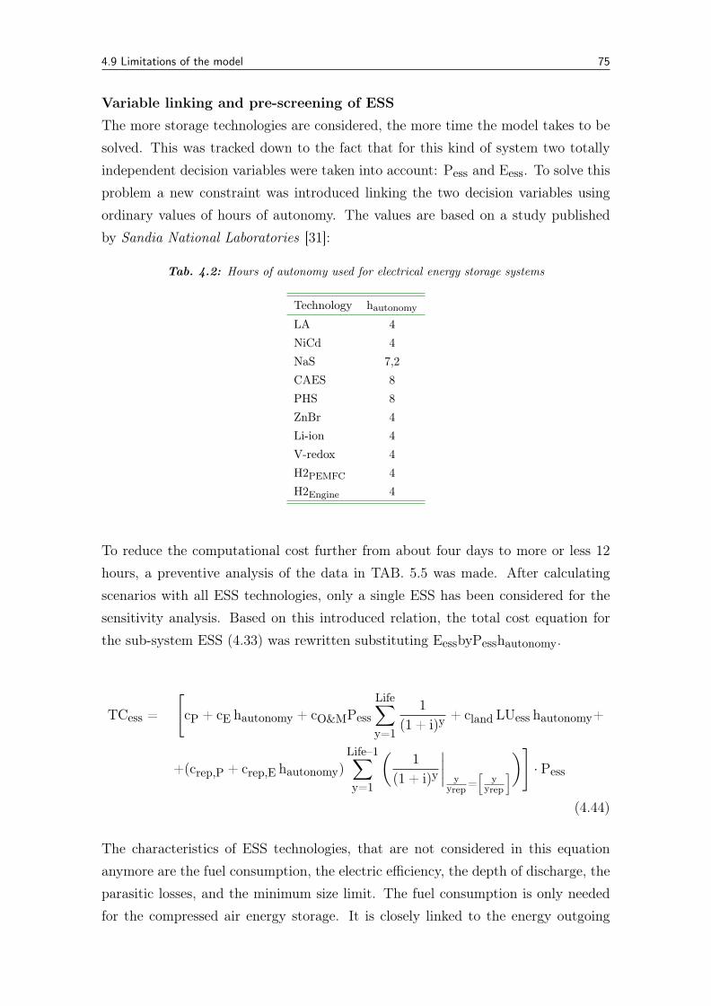
4.9 Limitations of the model 75
Variable linking and pre-screening of ESS
The more storage technologies are considered, the more time the model takes to besolved. This was tracked down to the fact that for this kind of system two totallyindependent decision variables were taken into account: Pess and Eess. To solve thisproblem a new constraint was introduced linking the two decision variables usingordinary values of hours of autonomy. The values are based on a study publishedby Sandia National Laboratories [31]:
Tab. 4.2: Hours of autonomy used for electrical energy storage systems
Technology hautonomy
LA 4NiCd 4NaS 7,2CAES 8PHS 8ZnBr 4Li-ion 4V-redox 4H2PEMFC 4H2Engine 4
To reduce the computational cost further from about four days to more or less 12hours, a preventive analysis of the data in TAB. 5.5 was made. After calculatingscenarios with all ESS technologies, only a single ESS has been considered for thesensitivity analysis. Based on this introduced relation, the total cost equation forthe sub-system ESS (4.33) was rewritten substituting EessbyPesshautonomy.
TCess =
[cP + cE hautonomy + cO&MPess
Life∑y=1
1(1 + i)y
+ cland LUess hautonomy+
+(crep,P + crep,E hautonomy)Life–1∑y=1
(1
(1 + i)y
∣∣∣∣ yyrep=
[y
yrep
])] · Pess
(4.44)
The characteristics of ESS technologies, that are not considered in this equationanymore are the fuel consumption, the electric efficiency, the depth of discharge, theparasitic losses, and the minimum size limit. The fuel consumption is only neededfor the compressed air energy storage. It is closely linked to the energy outgoing
76 Chapter 4 Model
fluxes and in case, CAES would be the optimal energy storage system, a furtheranalysis with the original model would need to be calculated, eliminating as manyother ESS technologies as possible.
The parasitic losses are very small for most technologies. They can be treated asefficiency losses, if a specific time period is set between charging and discharging.This way the losses can be eliminated from the main model and computational costscan slightly be minimized. Setting the time to 24 hours, the new efficiency can bewritten as
η* = η – Losses · 24 (4.45)
The depth of discharge affects the energy capacity of an electricity storage system.It can be lower than the rated capacity if DOD < 100%. However, from test calcu-lations it has been observed that the most important constraint for the optimizationis the rated power and not the installed capacity, so the DOD has little influence onthe choice of the storage system. Therefore neglecting the depth of discharge doesnot distort the optimal result significantly.
The pumped hydroelectric storage, the hydrogen-systems, the compressed air energysystem as well as the sodium-sulphur battery require a relatively high rated powerand are often dependent on geographical conditions, so that it needs to be decidedindividually, if they are applicable for a specific region and case or not.
4.9.4 Capacity of diesel generators
Due to the simplification requirements as previously mentioned, the diesel genera-tor sets are not free variables. There are only two options: One caterpillar dieselgenerator with a nominal capacity of 800 kWel can be in operation or two of themwith a total capacity of 1600 kWel. This static determination can distort the op-timal system design. E.g. when the demand changes in the sensitivity analysis,the model would maybe replace the diesel generator set by a larger one or installfurther ones, what is not possible in the model. A further drawback of this sim-plified approach is, that in real life projects, probably two smaller diesel generatorsets would be implemented instead of one large one. Two smaller ones can reactmore dynamic on the load curve than one large diesel generator. Most of the timethe diesel generator operates in part-load and performs not in the optimal capacity

4.9 Limitations of the model 77
range. Higher fuel consumption is the consequence and unfortunately the accuracyof the model shrinks. But to model the complex interaction between two dieselgenerators performing in their optimal capacity ratio, is beyond the scope of thismodel.
Chapter
5Case Study: A Cape Verde island
5.1 Background of Cape Verde
In this work an exemplary case study has been carried out for one of the Small IslandDeveloping States: a small island of the Cape Verde Islands named Brava. Whenlooked at from a global perspective, Cape Verde is one of the poorest countries eversince its independence from Portugal in 1975. Due to international projects andsupport, Cape Verde’s economic situation has improved during the past 30 years.
The island state Cape Verde consists of fifteen islands, nine of them inhabited, witha total land area of 4,036 km2 and a population of about 506,000. The Cape Verdeislands are volcanic and around 600 km away from the west coast of Africa (Senegal)in the Atlantic Ocean. Brava is the smallest inhabited, southernmost island of CapeVerde with a surface area of 67 km2 and about 6000 inhabitants, cf. Fig. 5.1 [105].
The islands can be divided into windward islands in the north and leeward islandsin the south (Maio, Santiago, Fogo and Brava). The capital, Praia, is locatedon Santiago, which is the largest island of Cape Verde. The island state is semi-dry to dry with relatively constant annual temperature averages from 24 to 29 ◦C.Water shortage is one of the main reasons behind its limited development. CapeVerde is highly dependent on oil imports, which are mainly used for electricitygeneration, air traffic and for daily use, e.g. cooking (kerosine or butane gas). Poweris supplied with 99 % by diesel generators. Currently the price of 1 kWh is 0.31e (forhigher consumption than 60 kWh/month) and 0.25 e/kWh respectively (for lowerconsumptions than 60 kWh/month) on Cape Verde [106]. ELECTRA provides notonly power but also water and sewerage services in Cape Verde. Water prices of2.35e/m3 (< 6 m3), 4.36e/m3 (>10 m3) and 4.93e/m3 for tourists and tourism
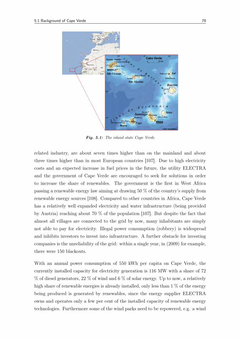
5.1 Background of Cape Verde 79
Fig. 5.1: The island state Cape Verde
related industry, are about seven times higher than on the mainland and aboutthree times higher than in most European countries [107]. Due to high electricitycosts and an expected increase in fuel prices in the future, the utility ELECTRAand the government of Cape Verde are encouraged to seek for solutions in orderto increase the share of renewables. The government is the first in West Africapassing a renewable energy law aiming at drawing 50 % of the country’s supply fromrenewable energy sources [108]. Compared to other countries in Africa, Cape Verdehas a relatively well expanded electricity and water infrastructure (being providedby Austria) reaching about 70 % of the population [107]. But despite the fact thatalmost all villages are connected to the grid by now, many inhabitants are simplynot able to pay for electricity. Illegal power consumption (robbery) is widespreadand inhibits investors to invest into infrastructure. A further obstacle for investingcompanies is the unreliability of the grid: within a single year, in (2009) for example,there were 150 blackouts.
With an annual power consumption of 550 kWh per capita on Cape Verde, thecurrently installed capacity for electricity generation is 116 MW with a share of 72% of diesel generators, 22 % of wind and 6 % of solar energy. Up to now, a relativelyhigh share of renewable energies is already installed, only less than 1 % of the energybeing produced is generated by renewables, since the energy supplier ELECTRAowns and operates only a few per cent of the installed capacity of renewable energytechnologies. Furthermore some of the wind parks need to be repowered, e.g. a wind
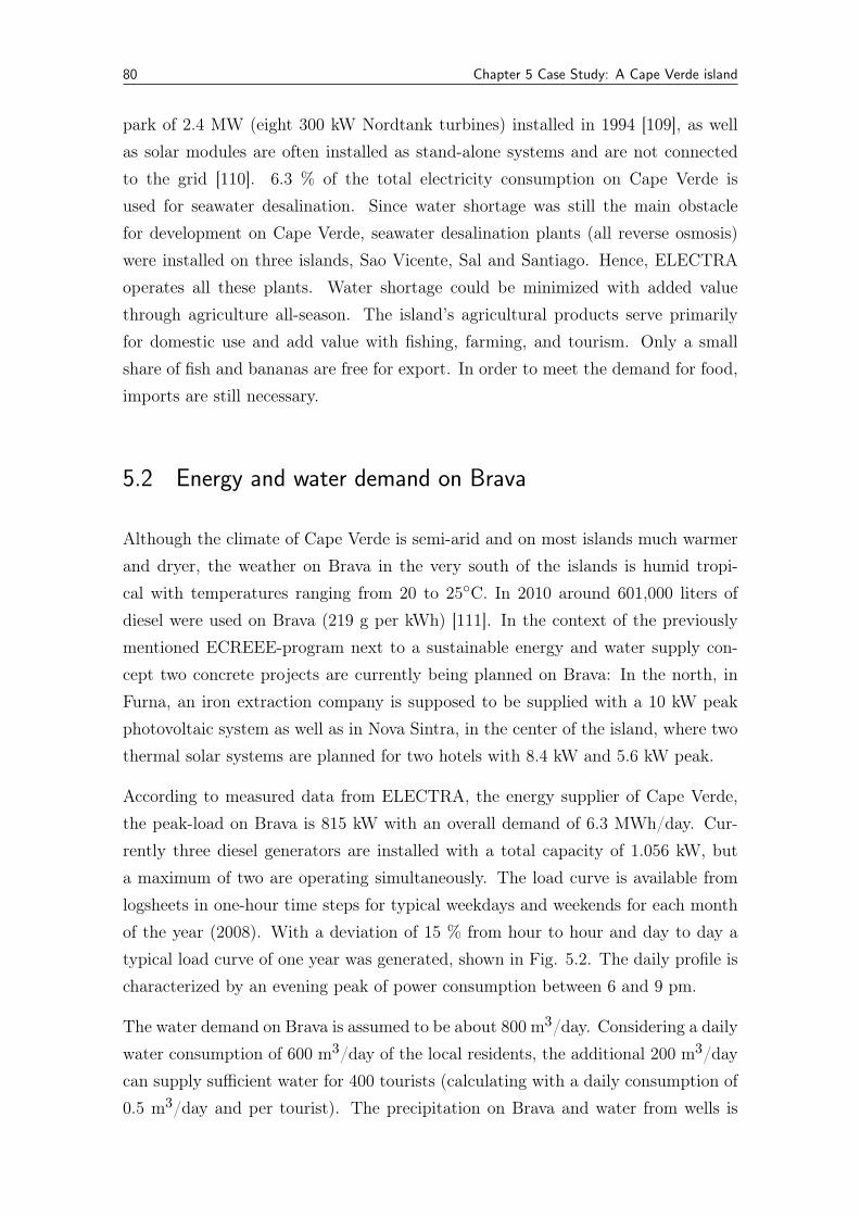
80 Chapter 5 Case Study: A Cape Verde island
park of 2.4 MW (eight 300 kW Nordtank turbines) installed in 1994 [109], as wellas solar modules are often installed as stand-alone systems and are not connectedto the grid [110]. 6.3 % of the total electricity consumption on Cape Verde isused for seawater desalination. Since water shortage was still the main obstaclefor development on Cape Verde, seawater desalination plants (all reverse osmosis)were installed on three islands, Sao Vicente, Sal and Santiago. Hence, ELECTRAoperates all these plants. Water shortage could be minimized with added valuethrough agriculture all-season. The island’s agricultural products serve primarilyfor domestic use and add value with fishing, farming, and tourism. Only a smallshare of fish and bananas are free for export. In order to meet the demand for food,imports are still necessary.
5.2 Energy and water demand on Brava
Although the climate of Cape Verde is semi-arid and on most islands much warmerand dryer, the weather on Brava in the very south of the islands is humid tropi-cal with temperatures ranging from 20 to 25◦C. In 2010 around 601,000 liters ofdiesel were used on Brava (219 g per kWh) [111]. In the context of the previouslymentioned ECREEE-program next to a sustainable energy and water supply con-cept two concrete projects are currently being planned on Brava: In the north, inFurna, an iron extraction company is supposed to be supplied with a 10 kW peakphotovoltaic system as well as in Nova Sintra, in the center of the island, where twothermal solar systems are planned for two hotels with 8.4 kW and 5.6 kW peak.
According to measured data from ELECTRA, the energy supplier of Cape Verde,the peak-load on Brava is 815 kW with an overall demand of 6.3 MWh/day. Cur-rently three diesel generators are installed with a total capacity of 1.056 kW, buta maximum of two are operating simultaneously. The load curve is available fromlogsheets in one-hour time steps for typical weekdays and weekends for each monthof the year (2008). With a deviation of 15 % from hour to hour and day to day atypical load curve of one year was generated, shown in Fig. 5.2. The daily profile ischaracterized by an evening peak of power consumption between 6 and 9 pm.
The water demand on Brava is assumed to be about 800 m3/day. Considering a dailywater consumption of 600 m3/day of the local residents, the additional 200 m3/daycan supply sufficient water for 400 tourists (calculating with a daily consumption of0.5 m3/day and per tourist). The precipitation on Brava and water from wells is
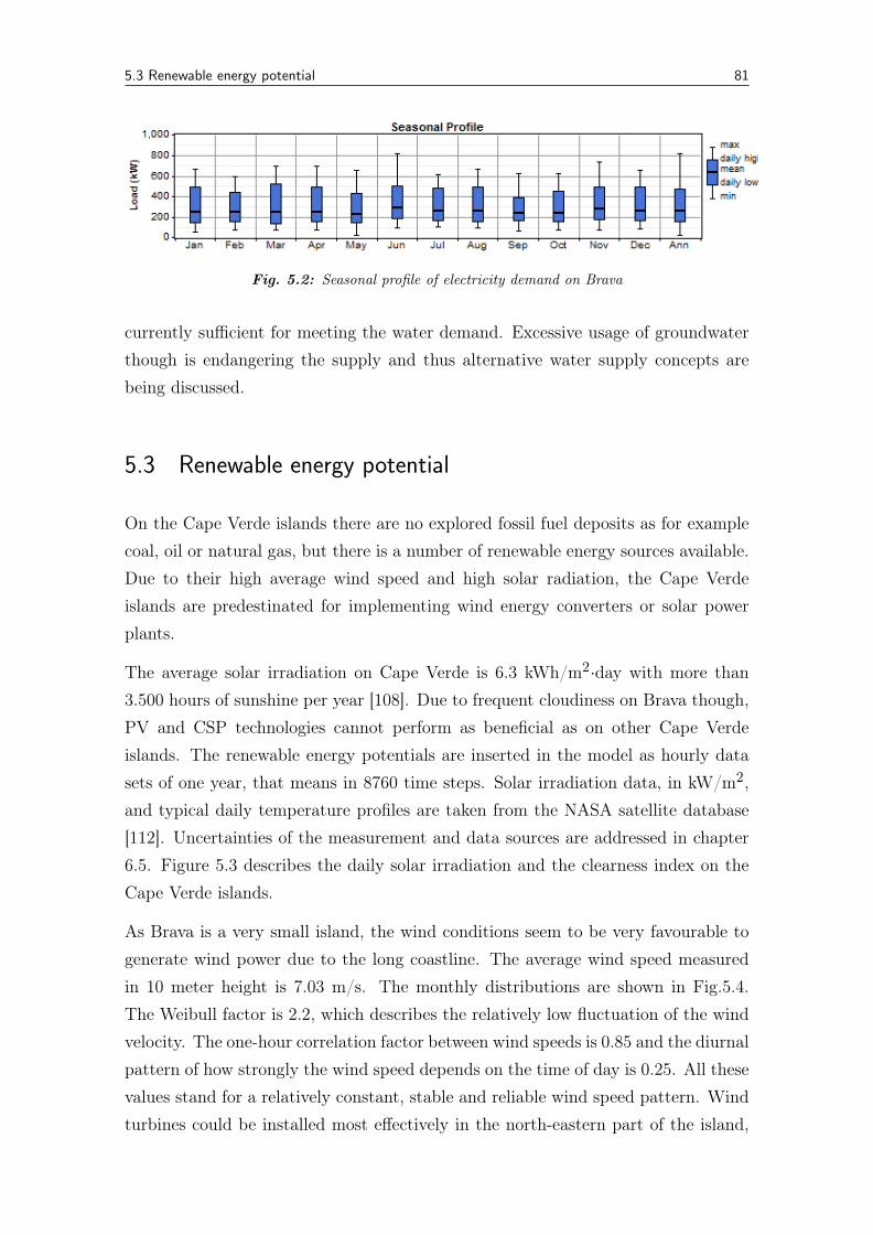
5.3 Renewable energy potential 81
Fig. 5.2: Seasonal profile of electricity demand on Brava
currently sufficient for meeting the water demand. Excessive usage of groundwaterthough is endangering the supply and thus alternative water supply concepts arebeing discussed.
5.3 Renewable energy potential
On the Cape Verde islands there are no explored fossil fuel deposits as for examplecoal, oil or natural gas, but there is a number of renewable energy sources available.Due to their high average wind speed and high solar radiation, the Cape Verdeislands are predestinated for implementing wind energy converters or solar powerplants.
The average solar irradiation on Cape Verde is 6.3 kWh/m2·day with more than3.500 hours of sunshine per year [108]. Due to frequent cloudiness on Brava though,PV and CSP technologies cannot perform as beneficial as on other Cape Verdeislands. The renewable energy potentials are inserted in the model as hourly datasets of one year, that means in 8760 time steps. Solar irradiation data, in kW/m2,and typical daily temperature profiles are taken from the NASA satellite database[112]. Uncertainties of the measurement and data sources are addressed in chapter6.5. Figure 5.3 describes the daily solar irradiation and the clearness index on theCape Verde islands.
As Brava is a very small island, the wind conditions seem to be very favourable togenerate wind power due to the long coastline. The average wind speed measuredin 10 meter height is 7.03 m/s. The monthly distributions are shown in Fig.5.4.The Weibull factor is 2.2, which describes the relatively low fluctuation of the windvelocity. The one-hour correlation factor between wind speeds is 0.85 and the diurnalpattern of how strongly the wind speed depends on the time of day is 0.25. All thesevalues stand for a relatively constant, stable and reliable wind speed pattern. Windturbines could be installed most effectively in the north-eastern part of the island,
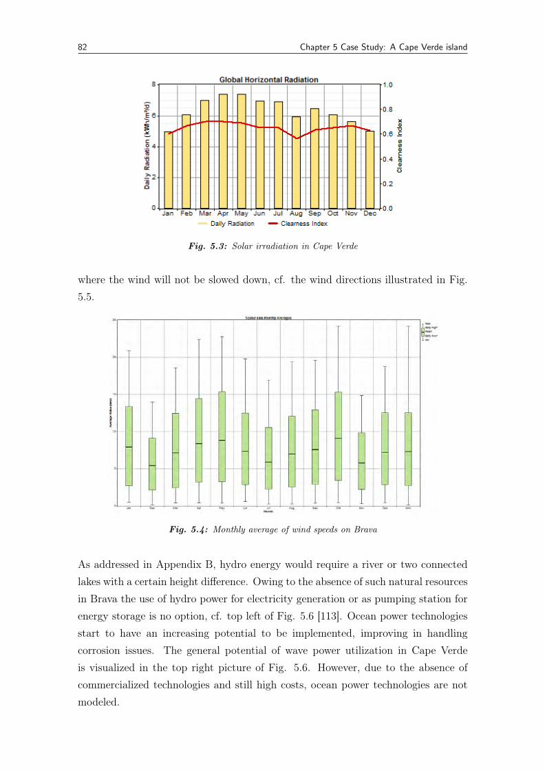
82 Chapter 5 Case Study: A Cape Verde island
Fig. 5.3: Solar irradiation in Cape Verde
where the wind will not be slowed down, cf. the wind directions illustrated in Fig.5.5.
Fig. 5.4: Monthly average of wind speeds on Brava
As addressed in Appendix B, hydro energy would require a river or two connectedlakes with a certain height difference. Owing to the absence of such natural resourcesin Brava the use of hydro power for electricity generation or as pumping station forenergy storage is no option, cf. top left of Fig. 5.6 [113]. Ocean power technologiesstart to have an increasing potential to be implemented, improving in handlingcorrosion issues. The general potential of wave power utilization in Cape Verdeis visualized in the top right picture of Fig. 5.6. However, due to the absence ofcommercialized technologies and still high costs, ocean power technologies are notmodeled.
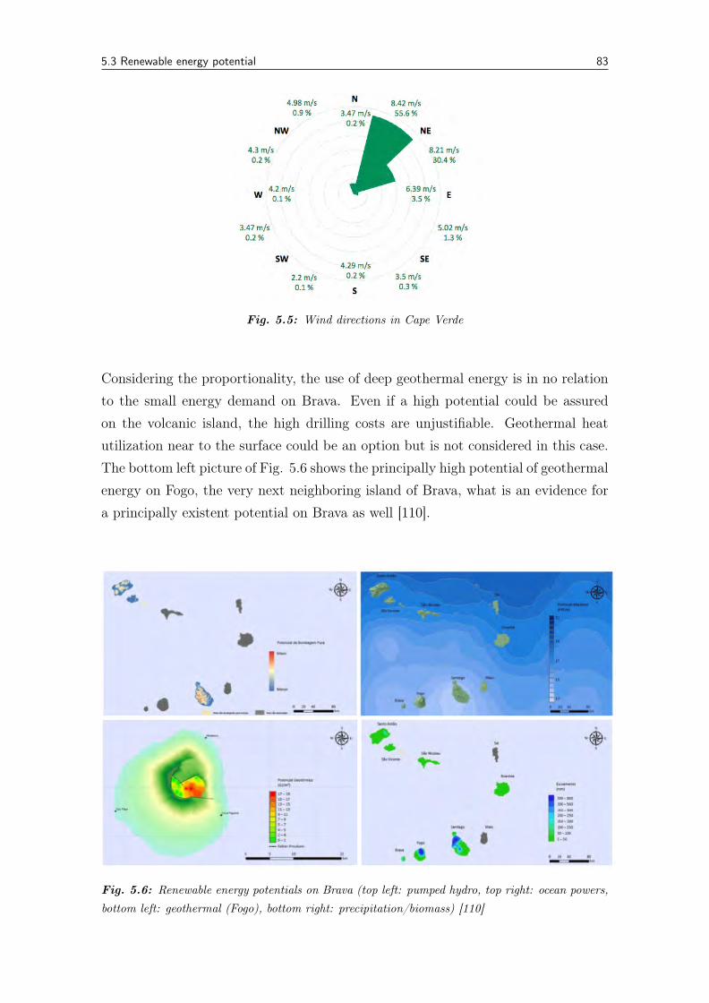
5.3 Renewable energy potential 83
Fig. 5.5: Wind directions in Cape Verde
Considering the proportionality, the use of deep geothermal energy is in no relationto the small energy demand on Brava. Even if a high potential could be assuredon the volcanic island, the high drilling costs are unjustifiable. Geothermal heatutilization near to the surface could be an option but is not considered in this case.The bottom left picture of Fig. 5.6 shows the principally high potential of geothermalenergy on Fogo, the very next neighboring island of Brava, what is an evidence fora principally existent potential on Brava as well [110].
Fig. 5.6: Renewable energy potentials on Brava (top left: pumped hydro, top right: ocean powers,bottom left: geothermal (Fogo), bottom right: precipitation/biomass) [110]
84 Chapter 5 Case Study: A Cape Verde island
Biomass as another potential energy source is neither being considered, since thenatural vegetation is not sufficient for such an utilization. Since even the agricul-tural demand for domestic use cannot be met, cultured energy crops are no option.Advancing the mass and energetic recovery of farmed algae can be a support as bio-fuel in the future, but is beyond the scope of this research. The bottom right pictureof Fig. 5.6 confirms the low precipitation and low potential of biomass utilizationon Cape Verde.
5.4 Input data in the model
5.4.1 Economic input data
The lifetime and investment period of almost all components is set to 20 years,only the energy storage systems vary significantly in their lifetimes. To evaluate theeconomic performance of the project an interest rate of 5 % is being employed. Theexchange rate between the US-Dollar and the Euro is considered with an averageof 1.3 USD = 1e. All other currencies are also converted to Euro. Fuel pricesare assumed to be constant for the whole lifetime period. The effect of varyingdiesel prices is addressed later within the scenario and real option analyses. A verymoderate diesel price of 0.07e per liter is assumed initially. In the model the unit forthe diesel price is e/kWh. Based on the heating rate, the liter-price divided by 9.7kWh/liter, results in a diesel price of 0.072e/kWh. The cost of natural gas used inthe Compressed Air Energy Storage system is amounting to 0.06e/kWh [114]. Theprice of CO2-equivalents is set to a currently unrealistically high price of 20e/t CO2.The specific emission of diesel fuel is 0,248 kg CO2/kWh, adopted from the specificvolumetric emission of diesel fuel multiplied by the volumetric energy density. Incase that the Compressed Air Energy Storage system is part of the optimal solution,the specific emission of the natural gas is 0,179 kg CO2/kWh [115]. The price forland is set to 30e/m2, which is the mean value of real estate prices on the CapeVerde islands.
5.4.2 Input data PV-systems
Three different technologies of photovoltaic panels are taken into consideration: amulti-crystalline, wafer based silicon technology (c-Si), an amorphous micro-crystallinesilicon technology (a-Si) as well as a cadmium telluride technology (CdTe). Detailed
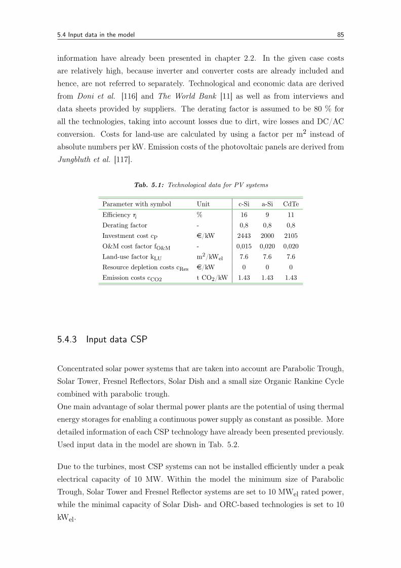
5.4 Input data in the model 85
information have already been presented in chapter 2.2. In the given case costsare relatively high, because inverter and converter costs are already included andhence, are not referred to separately. Technological and economic data are derivedfrom Doni et al. [116] and The World Bank [11] as well as from interviews anddata sheets provided by suppliers. The derating factor is assumed to be 80 % forall the technologies, taking into account losses due to dirt, wire losses and DC/ACconversion. Costs for land-use are calculated by using a factor per m2 instead ofabsolute numbers per kW. Emission costs of the photovoltaic panels are derived fromJungbluth et al. [117].
Tab. 5.1: Technological data for PV systems
Parameter with symbol Unit c-Si a-Si CdTe
Efficiency η % 16 9 11Derating factor - 0,8 0,8 0,8Investment cost cP e/kW 2443 2000 2105O&M cost factor fO&M - 0,015 0,020 0,020Land-use factor kLU m2/kWel 7.6 7.6 7.6Resource depletion costs cRes e/kW 0 0 0Emission costs cCO2 t CO2/kW 1.43 1.43 1.43
5.4.3 Input data CSP
Concentrated solar power systems that are taken into account are Parabolic Trough,Solar Tower, Fresnel Reflectors, Solar Dish and a small size Organic Rankine Cyclecombined with parabolic trough.One main advantage of solar thermal power plants are the potential of using thermalenergy storages for enabling a continuous power supply as constant as possible. Moredetailed information of each CSP technology have already been presented previously.Used input data in the model are shown in Tab. 5.2.
Due to the turbines, most CSP systems can not be installed efficiently under a peakelectrical capacity of 10 MW. Within the model the minimum size of ParabolicTrough, Solar Tower and Fresnel Reflector systems are set to 10 MWel rated power,while the minimal capacity of Solar Dish- and ORC-based technologies is set to 10kWel.
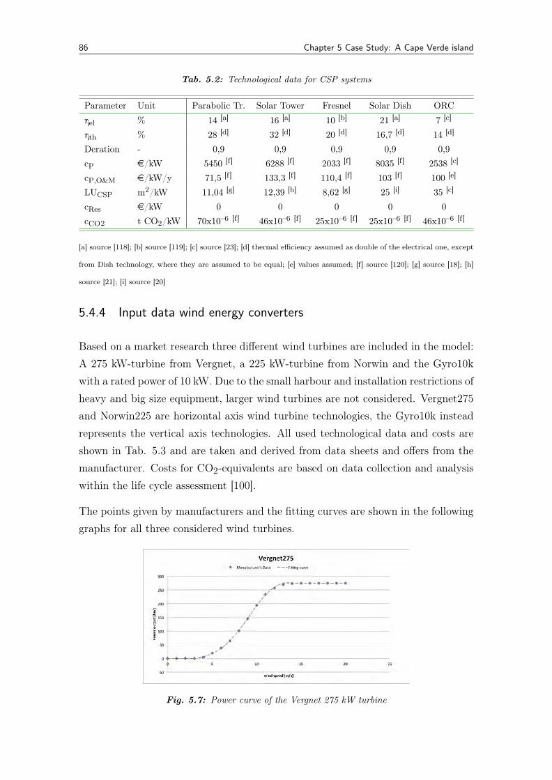
86 Chapter 5 Case Study: A Cape Verde island
Tab. 5.2: Technological data for CSP systems
Parameter Unit Parabolic Tr. Solar Tower Fresnel Solar Dish ORC
ηel % 14 [a] 16 [a] 10 [b] 21 [a] 7 [c]
ηth % 28 [d] 32 [d] 20 [d] 16,7 [d] 14 [d]
Deration - 0,9 0,9 0,9 0,9 0,9cP e/kW 5450 [f] 6288 [f] 2033 [f] 8035 [f] 2538 [c]
cP,O&M e/kW/y 71,5 [f] 133,3 [f] 110,4 [f] 103 [f] 100 [e]
LUCSP m2/kW 11,04 [g] 12,39 [h] 8,62 [g] 25 [i] 35 [c]
cRes e/kW 0 0 0 0 0cCO2 t CO2/kW 70x10–6 [f] 46x10–6 [f] 25x10–6 [f] 25x10–6 [f] 46x10–6 [f]
[a] source [118]; [b] source [119]; [c] source [23]; [d] thermal efficiency assumed as double of the electrical one, except
from Dish technology, where they are assumed to be equal; [e] values assumed; [f] source [120]; [g] source [18]; [h]
source [21]; [i] source [20]
5.4.4 Input data wind energy converters
Based on a market research three different wind turbines are included in the model:A 275 kW-turbine from Vergnet, a 225 kW-turbine from Norwin and the Gyro10kwith a rated power of 10 kW. Due to the small harbour and installation restrictions ofheavy and big size equipment, larger wind turbines are not considered. Vergnet275and Norwin225 are horizontal axis wind turbine technologies, the Gyro10k insteadrepresents the vertical axis technologies. All used technological data and costs areshown in Tab. 5.3 and are taken and derived from data sheets and offers from themanufacturer. Costs for CO2-equivalents are based on data collection and analysiswithin the life cycle assessment [100].
The points given by manufacturers and the fitting curves are shown in the followinggraphs for all three considered wind turbines.
Fig. 5.7: Power curve of the Vergnet 275 kW turbine
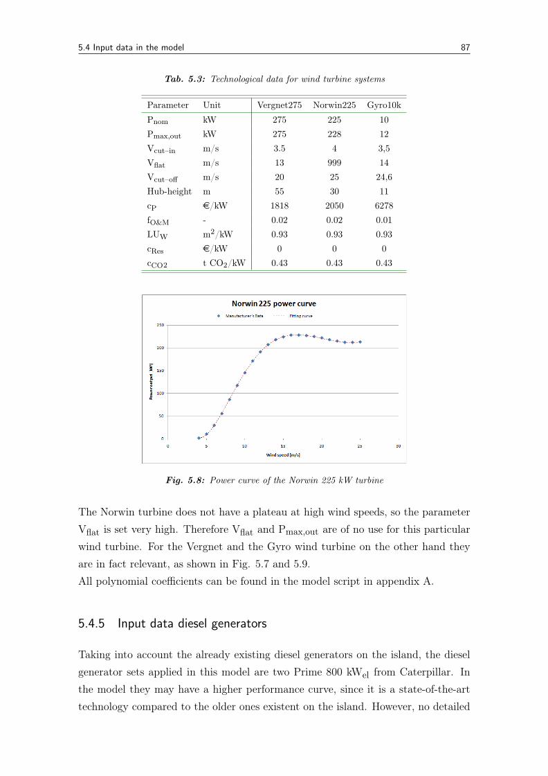
5.4 Input data in the model 87
Tab. 5.3: Technological data for wind turbine systems
Parameter Unit Vergnet275 Norwin225 Gyro10k
Pnom kW 275 225 10Pmax,out kW 275 228 12Vcut–in m/s 3.5 4 3,5Vflat m/s 13 999 14Vcut–off m/s 20 25 24,6Hub-height m 55 30 11cP e/kW 1818 2050 6278fO&M - 0.02 0.02 0.01LUW m2/kW 0.93 0.93 0.93cRes e/kW 0 0 0cCO2 t CO2/kW 0.43 0.43 0.43
Fig. 5.8: Power curve of the Norwin 225 kW turbine
The Norwin turbine does not have a plateau at high wind speeds, so the parameterVflat is set very high. Therefore Vflat and Pmax,out are of no use for this particularwind turbine. For the Vergnet and the Gyro wind turbine on the other hand theyare in fact relevant, as shown in Fig. 5.7 and 5.9.All polynomial coefficients can be found in the model script in appendix A.
5.4.5 Input data diesel generators
Taking into account the already existing diesel generators on the island, the dieselgenerator sets applied in this model are two Prime 800 kWel from Caterpillar. Inthe model they may have a higher performance curve, since it is a state-of-the-arttechnology compared to the older ones existent on the island. However, no detailed
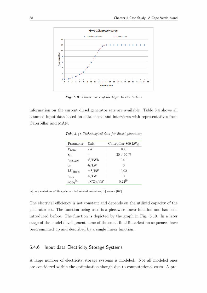
88 Chapter 5 Case Study: A Cape Verde island
Fig. 5.9: Power curve of the Gyro 10 kW turbine
information on the current diesel generator sets are available. Table 5.4 shows allassumed input data based on data sheets and interviews with representatives fromCaterpillar and MAN.
Tab. 5.4: Technological data for diesel generators
Parameter Unit Caterpillar 800 kWel
Pnom kW 800ηth - 30 / 60 %cE,O&M e/kWh 0.01cP e/kW 0LUdiesel m2/kW 0.02cRes e/kW 0cCO2
[a] t CO2/kW 0.22[b]
[a] only emissions of life cycle, no fuel related emissions; [b] source [100]
The electrical efficiency is not constant and depends on the utilized capacity of thegenerator set. The function being used is a piecewise linear function and has beenintroduced before. The function is depicted by the graph in Fig. 5.10. In a laterstage of the model development some of the small final linearization sequences havebeen summed up and described by a single linear function.
5.4.6 Input data Electricity Storage Systems
A large number of electricity storage systems is modeled. Not all modeled onesare considered within the optimization though due to computational costs. A pre-
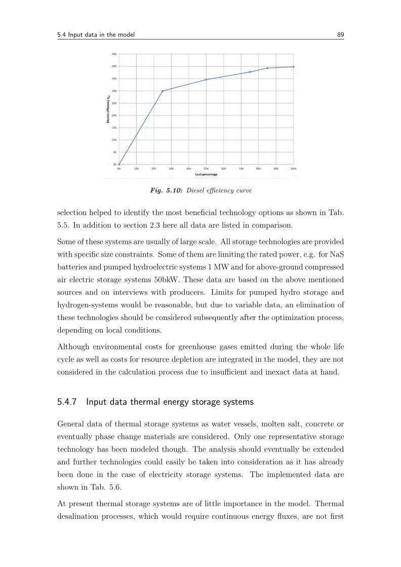
5.4 Input data in the model 89
Fig. 5.10: Diesel efficiency curve
selection helped to identify the most beneficial technology options as shown in Tab.5.5. In addition to section 2.3 here all data are listed in comparison.
Some of these systems are usually of large scale. All storage technologies are providedwith specific size constraints. Some of them are limiting the rated power, e.g. for NaSbatteries and pumped hydroelectric systems 1 MW and for above-ground compressedair electric storage systems 50bkW. These data are based on the above mentionedsources and on interviews with producers. Limits for pumped hydro storage andhydrogen-systems would be reasonable, but due to variable data, an elimination ofthese technologies should be considered subsequently after the optimization process,depending on local conditions.
Although environmental costs for greenhouse gases emitted during the whole lifecycle as well as costs for resource depletion are integrated in the model, they are notconsidered in the calculation process due to insufficient and inexact data at hand.
5.4.7 Input data thermal energy storage systems
General data of thermal storage systems as water vessels, molten salt, concrete oreventually phase change materials are considered. Only one representative storagetechnology has been modeled though. The analysis should eventually be extendedand further technologies could easily be taken into consideration as it has alreadybeen done in the case of electricity storage systems. The implemented data areshown in Tab. 5.6.
At present thermal storage systems are of little importance in the model. Thermaldesalination processes, which would require continuous energy fluxes, are not first
90 Chapter 5 Case Study: A Cape Verde island
Tab. 5.5: Technological data for electricity storage systems
Parameter Unit LA NiCd NaS CAES PHS
cP e/kW 195,97[a] 195,97[a] 130,65[a] 522,60[a] 914,54[a]
cE e/kWh 130,65[a] 522,60[a] 217,75[a] 104,52[a] 12,19[a]
η - 75%[a] 65%[a] 7%[a] 79%[a] 78%[a]
crep,P e/kW 0[a] 0[a] 0[a] 0[a] 0[a]
crep,E e/kWh 130,65[a] 522,60[a] 200,33[a] 0[a] 0[a]
yrep y 6[a] 10[a] 15[a] 30[b] 50[b]
DOD - 75%[c] 100%[c] 100%[c] 62,5%[e] 95%[e]
Consfuel - 0 0 0 1,29[d] 0cO&M e/kW/y 15[a] 25[a] 20[a] 10[a] 2,5[a]
Losses 1/h 8,33E-07[f] 1,67E-06[f] 8,34E-05[f] 0[f] 0[f]
LUess m2/kWh 0,058[h] 0,042[g] 0,037[i] 0,214[h] 0,186[h]
Parameter Unit ZnBr Li-ion V-redox H2PEMFC H2EnginecP e/kW 152,42[a] 152,42[a] 178,55[a] 1567,79[a] 261,30[a]
cE e/kWh 348,40[a] 435,50[a] 522,60[a] 13,06[a] 13,06[a]
η - 60%[a] 85%[a] 70%[a] 53%[a] 44%[a]
crep,P e/kW 0[a] 0[a] 0[a] 130,65[a] 95,81[a]
crep,E e/kWh 87,10[a] 435,50[a] 522,60[a] 0[a] 0[a]
yrep y 8[a] 10[a] 10[a] 6[a] 6[a]
DOD - 100%[c] 80%[c] 100%[d] 90%[e] 90%[e]
Consfuel - 0 0 0 0 0cO&M e/kW/y 20[a] 25[a] 20[a] 3,8[a] 2,5[a]
Losses 1/h 0[f] 8,33E-07[f] 0[f] 0[f] 0[f]
LUess m2/kWh 0,023[h] 0,010[g] 0,037[i] 0,042[h] 0,005[h]
[a] source [30], costs actualized using Consumer Price Index[121]; [b] source [29]; [c] source [102]; [d] source [122]; [e]
source [103]; [f] source [123]; [g] Manufacturer manual & environmental assessments; [h] source [31]; [i] source [124]
choice on an electrified island. Environmental and land-use costs of thermal energystorages are not considered.
5.4.8 Input data Desalination
Taking on the technological backgrounds from desalination technologies in chapter2.5, the detailed energy consumptions and costs of each considered process are com-piled in Tab. 5.7. All data are based on information from manufacturers of eachdesalination technology and are verified. However, increases in energy efficiency andcost reductions are expectable in near future due to continuous development.
5.4 Input data in the model 91
Tab. 5.6: Technological data for thermal storage systems
Parameter Unit TSS
cE e/kWh 115η - 0,9cO&M e/kWh/y 5Losses h–1 1,00E-05
Tab. 5.7: Technological data for desalination systems
Parameter Unit HDH MED MD MVC RO var-RO
Econs,th kWh/m3 100[a] 110[b] 175[c] 0[d] 0[e] 0Econs,el kWh/m3 2.4[a] 1.7[b] 0.1[c] 11[d] 4[e] variablecplant e/(m3/d) 3000[a] 3400[b] 5000[c] 2350[e] 2000[e] 2200[g]
cw,O&M e/m3 0.18[a] 0.16[b] 0.2[c] 0.29[d] 1.04[e] 1.04[g]
LUdesal m2/(m3/d) 0.3[a] 0.2[b] 0.3[c] 0.3[d] 0.3[e] 0.3[e]
[a] source [40] [b] source [76]; [c] source [46]; [d] source [47]; [e] source [54].
All technologies require electrical energy, even if some desalination processes aremainly thermally driven. Power is needed in these processes for operating waterpumps and auxiliary systems. A minimum capacity of 50 m3/d is set for all desali-nation processes, in order to avoid unrealistically small capacities. Environmentalcosts for greenhouse gases emitted during the whole life cycle of the desalinationplants as well as costs for resource depletion are modeled but set to zero due toinadequate data.
5.4.9 Input data water storage system
The considered water storage is nothing else than a water tank where water is beingstored in times of surplus freshwater production and from where it is taken fromin periods with less water production than is in fact needed. As mentioned before,only one representative type has been applied to the model. The water storage costis set to 180e/m3 and its land use factor is 0,5 m2 of surface occupied for every m3
of stored water. Both values are estimated by using the mean value of manufacturerdata.
Chapter
6Results
Energy and water supply systems were exemplary calculated and determined forvarious islands. The following results and detailed analysis though are accomplishedonly for the Cape Verde island Brava. Nevertheless, a summary of the simulationand optimization results of further islands can be found in chapter 6.7.
6.1 Validation of model
Before analyzing the results in more detail comparable parts of the GAMS model arevalidated by means of results of the commercial available energy system simulationtool HOMER. Differences between both calculation methods are, that HOMERis commonly considering a single technology in the framework of the optimization.Desalination, concentrated solar power as well as a number of energy storage systemscannot be modeled in HOMER. Usually within the optimization only one primaryselected power generation or storage technology is considered. In any case, thetechnology needs to be chosen in advance. An optimization concerning the optimalwind converter technology for a specific region e.g., cannot be calculated in HOMER.Therefore also in the GAMS model a comparable set of components is considered.(Converter costs are allocated and covered by the PV and battery costs respectively.)
For the validation common commercial multi-crystalline PV modules were consid-ered, 275 kW Vergnet wind turbines, 800 kW caterpillar diesel generators and con-ventional lead-acid batteries, in this case Hoppecke OPzS 3000 with a capacity of 6kWh. Within the GAMS model other generation and storage technologies have beenoutlined for identifying differences between the two optimization approaches. Table6.1 and 6.2 show the optimal supply systems for Brava calculated with HOMER and
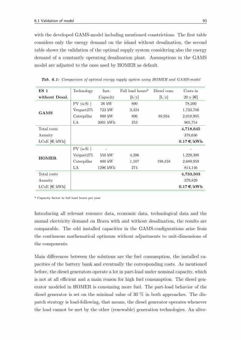
6.1 Validation of model 93
with the developed GAMS-model including mentioned constrictions. The first tableconsiders only the energy demand on the island without desalination, the secondtable shows the validation of the optimal supply system considering also the energydemand of a constantly operating desalination plant. Assumptions in the GAMSmodel are adjusted to the ones used by HOMER as default.
Tab. 6.1: Comparison of optimal energy supply system using HOMER and GAMS-model
ES 1 Technology Inst. Full load hours* Diesel cons. Costs inwithout Desal. Capacity [h/y] [L/y] 20 y [e]
GAMS
PV (a-Si ) 26 kW 890 78,200Vergnet275 723 kW 3,324 1,723,786Caterpillar 800 kW 806 88,934 2,010,905LA 2001 kWh 253 905,754
Total costs 4,718,645Annuity 378,636LCoE [e/kWh] 0.17e/kWh
HOMER
PV (a-Si ) - -Vergnet275 550 kW 4,396 1,229,398Caterpillar 800 kW 1,107 198,316 2,689,959LA 1296 kWh 274 814,146
Total costs 4,733,503Annuity 379,829LCoE [e/kWh] 0.17e/kWh
* Capacity factor in full load hours per year
Introducing all relevant resource data, economic data, technological data and theannual electricity demand on Brava with and without desalination, the results arecomparable. The odd installed capacities in the GAMS-configurations arise fromthe continuous mathematical optimum without adjustments to unit-dimensions ofthe components.
Main differences between the solutions are the fuel consumption, the installed ca-pacities of the battery bank and eventually the corresponding costs. As mentionedbefore, the diesel generators operate a lot in part-load under nominal capacity, whichis not at all efficient and a main reason for high fuel consumption. The diesel gen-erator modeled in HOMER is consuming more fuel. The part-load behavior of thediesel generator is set on the minimal value of 30 % in both approaches. The dis-patch strategy is load-following, that means, the diesel generator operates wheneverthe load cannot be met by the other (renewable) generation technologies. An alter-
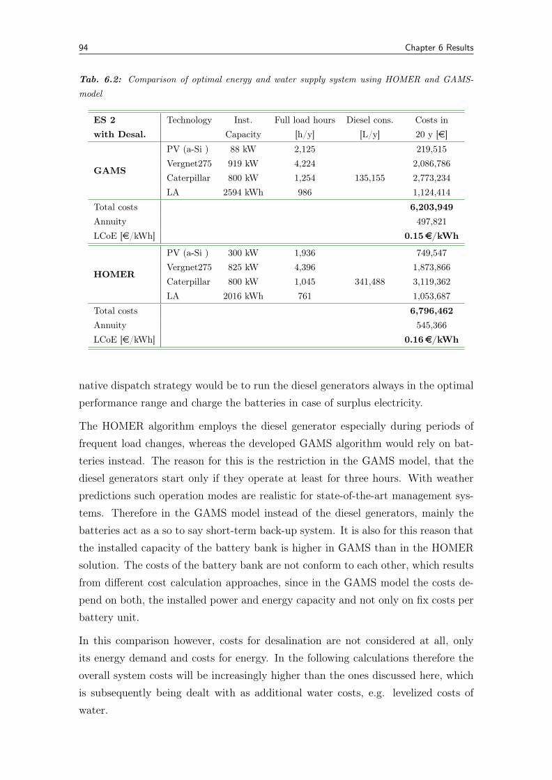
94 Chapter 6 Results
Tab. 6.2: Comparison of optimal energy and water supply system using HOMER and GAMS-model
ES 2 Technology Inst. Full load hours Diesel cons. Costs inwith Desal. Capacity [h/y] [L/y] 20 y [e]
GAMS
PV (a-Si ) 88 kW 2,125 219,515Vergnet275 919 kW 4,224 2,086,786Caterpillar 800 kW 1,254 135,155 2,773,234LA 2594 kWh 986 1,124,414
Total costs 6,203,949Annuity 497,821LCoE [e/kWh] 0.15e/kWh
HOMER
PV (a-Si ) 300 kW 1,936 749,547Vergnet275 825 kW 4,396 1,873,866Caterpillar 800 kW 1,045 341,488 3,119,362LA 2016 kWh 761 1,053,687
Total costs 6,796,462Annuity 545,366LCoE [e/kWh] 0.16e/kWh
native dispatch strategy would be to run the diesel generators always in the optimalperformance range and charge the batteries in case of surplus electricity.
The HOMER algorithm employs the diesel generator especially during periods offrequent load changes, whereas the developed GAMS algorithm would rely on bat-teries instead. The reason for this is the restriction in the GAMS model, that thediesel generators start only if they operate at least for three hours. With weatherpredictions such operation modes are realistic for state-of-the-art management sys-tems. Therefore in the GAMS model instead of the diesel generators, mainly thebatteries act as a so to say short-term back-up system. It is also for this reason thatthe installed capacity of the battery bank is higher in GAMS than in the HOMERsolution. The costs of the battery bank are not conform to each other, which resultsfrom different cost calculation approaches, since in the GAMS model the costs de-pend on both, the installed power and energy capacity and not only on fix costs perbattery unit.
In this comparison however, costs for desalination are not considered at all, onlyits energy demand and costs for energy. In the following calculations therefore theoverall system costs will be increasingly higher than the ones discussed here, whichis subsequently being dealt with as additional water costs, e.g. levelized costs ofwater.
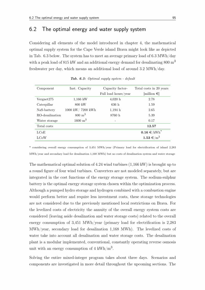
6.2 The optimal energy and water supply system 95
6.2 The optimal energy and water supply system
Considering all elements of the model introduced in chapter 4, the mathematicaloptimal supply system for the Cape Verde island Brava might look like as depictedin Tab. 6.3 below. The system has to meet an average primary load of 6.3 MWh/daywith a peak load of 815 kW and an additional energy demand for desalinating 800 m3
freshwater per day, which means an additional load of around 3.2 MWh/day.
Tab. 6.3: Optimal supply system - default
Component Inst. Capacity Capacity factor- Total costs in 20 yearsFull load hours/year [million e]
Vergnet275 1,166 kW 4,020 h 2.78Caterpillar 800 kW 636 h 1.59NaS-battery 1000 kW/ 7200 kWh 1,194 h 2.65RO-desalination 800 m3 8760 h 5.39Water storage 1600 m3 - 0.17
Total costs 12.57
LCoE 0.16 e/kWh*
LCoW 1.53 e/m3
* considering overall energy consumption of 3,451 MWh/year (Primary load for electrification of island 2,283
MWh/year and secondary load for desalination 1,168 MWh) but no costs of desalination system and water storage
The mathematical optimal solution of 4.24 wind turbines (1,166 kW) is brought up toa round figure of four wind turbines. Converters are not modeled separately, but areintegrated in the cost functions of the energy storage system. The sodium-sulphurbattery is the optimal energy storage system chosen within the optimization process.Although a pumped hydro storage and hydrogen combined with a combustion enginewould perform better and require less investment costs, these storage technologiesare not considered due to the previously mentioned local restrictions on Brava. Forthe levelized costs of electricity the annuity of the overall energy system costs areconsidered (leaving aside desalination and water storage costs) related to the overallenergy consumption of 3,451 MWh/year (primary load for electrification is 2,283MWh/year, secondary load for desalination 1,168 MWh). The levelized costs ofwater take into account all desalination and water storage costs. The desalinationplant is a modular implemented, conventional, constantly operating reverse osmosisunit with an energy consumption of 4 kWh/m3.
Solving the entire mixed-integer program takes about three days. Scenarios andcomponents are investigated in more detail throughout the upcoming sections. The

96 Chapter 6 Results
majority of the limitation controls are employed, excluding irrelevant componentsof the model and minimizing computing costs without affecting the accuracy of theresult.
6.3 Supply scenarios in comparison
Depending on the demand on an inland, in this case on the Cape Verde islandBrava, different supply scenarios can be considered. In order to understand whateffect renewable energies would have on the current system and how desalinationcould contribute to such a specific energy generation mix, several energy systemsare looked at in detail:
ES 0: Business as usual, current systemES 1: Energy supply onlyES 2: Energy and water supply with conventional operating desalination plantES 3: Energy and water supply with variable operating desalination plant
For a better understanding of the effect of desalination on the energy supply system,no installation changes on the supply side are done. The recommended nominalcapacities of energy system 1 (ES 1) are also being used for ES 2 and ES 3. Thecalculations and analyses are based on a joint research work with Pohl as publishedin Bognar et al. [57]. The scenarios are calculated with the developed model, butusing a conventional lead acid-battery as default, which has no minimal installedcapacities and can therefore be implemented more flexible.
6.3.1 Integrating renewable energies into the current supply system
Energy system zero (ES 0) stands for the current energy system using only dieselgenerators. Table 6.4 shows the optimal installed capacities and costs of relevantcomponents of each scenario.
In scenario ES 1 it is assumed, that Brava can meet its water demand by using partlygroundwater and partly desalinated water from the neighboring islands, presumingthese islands have an over-capacity. In this case expensive water imports from themainland or desalination on site are not needed. The optimal energy supply is basedon a mixture of renewable and fossil energy sources, in this case three Vergnet windturbines with a nominal capacity of 275 kW per turbine and two Caterpillar dieselgenerators with a rated power of 800 kWel respectively. Generally, a single generator
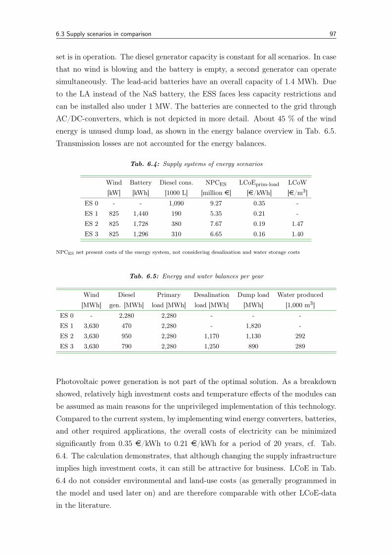
6.3 Supply scenarios in comparison 97
set is in operation. The diesel generator capacity is constant for all scenarios. In casethat no wind is blowing and the battery is empty, a second generator can operatesimultaneously. The lead-acid batteries have an overall capacity of 1.4 MWh. Dueto the LA instead of the NaS battery, the ESS faces less capacity restrictions andcan be installed also under 1 MW. The batteries are connected to the grid throughAC/DC-converters, which is not depicted in more detail. About 45 % of the windenergy is unused dump load, as shown in the energy balance overview in Tab. 6.5.Transmission losses are not accounted for the energy balances.
Tab. 6.4: Supply systems of energy scenarios
Wind Battery Diesel cons. NPCES LCoEprim-load LCoW[kW] [kWh] [1000 L] [million e] [e/kWh] [e/m3]
ES 0 - - 1,090 9.27 0.35 -ES 1 825 1,440 190 5.35 0.21 -ES 2 825 1,728 380 7.67 0.19 1.47ES 3 825 1,296 310 6.65 0.16 1.40
NPCES net present costs of the energy system, not considering desalination and water storage costs
Tab. 6.5: Energy and water balances per year
Wind Diesel Primary Desalination Dump load Water produced[MWh] gen. [MWh] load [MWh] load [MWh] [MWh] [1,000 m3]
ES 0 - 2,280 2,280 - - -ES 1 3,630 470 2,280 - 1,820 -ES 2 3,630 950 2,280 1,170 1,130 292ES 3 3,630 790 2,280 1,250 890 289
Photovoltaic power generation is not part of the optimal solution. As a breakdownshowed, relatively high investment costs and temperature effects of the modules canbe assumed as main reasons for the unprivileged implementation of this technology.Compared to the current system, by implementing wind energy converters, batteries,and other required applications, the overall costs of electricity can be minimizedsignificantly from 0.35 e/kWh to 0.21 e/kWh for a period of 20 years, cf. Tab.6.4. The calculation demonstrates, that although changing the supply infrastructureimplies high investment costs, it can still be attractive for business. LCoE in Tab.6.4 do not consider environmental and land-use costs (as generally programmed inthe model and used later on) and are therefore comparable with other LCoE-datain the literature.
98 Chapter 6 Results
Gaining increasing independence from oil imports and, therefore, stable energy pricesin the long-term represents beneficial opportunities of ES 1. There is also a clearecological benefit: by introducing renewable energy technologies to the current sup-ply system (scenario ES 1), 895,789 liter of diesel could be saved and about 2160tons of CO2-emissions cut down.
Analyzing the deviation of every hour within the one-year simulation of ES 1, aremarkable excess of electricity, generated by the wind turbines, is unused, cf. Tab.6.5. Especially in dry regions, using the dump load for water production, supple-menting existing water stocks, can be a beneficial solution.
Fig. 6.1: Desalination potential by excess wind electricity
Figure 6.1 shows the potential of water production only by wind energy surplus onthe island Brava. The light green area in the background is illustrating the excesswind energy generated in ES 1. The dark green bars in the front symbolize thepotential of freshwater production per week by the surplus wind energy, taking intoconsideration capacity constraints of an applicable desalination plant (maximumproduction rate 33 m3 freshwater per hour). The weekly freshwater demand onBrava is 5,600 m3. As it can be seen, only a few weeks this amount can be providedjust by excess wind energy, without having taken into consideration water storagetanks and alternative energy sources as back up technology. Figure 6.1 exemplifies,that excess electricity by renewable energies is able to meet a significant energy
6.3 Supply scenarios in comparison 99
demand of a desalination plant as considered here. However, it also proves that windenergy alone cannot guarantee a continuous and reliable water supply throughoutthe whole year and back up technologies are required.
6.3.2 The optimal desalination process
Motivated by the fact of excess electricity by integrated renewable energies, theintegration of desalination as additional load is looked at in more detail in scenariosES 2 and ES 3. From the five desalination processes considered in the model anddescribed in chapter 2.5 in this particular case a commonly used reverse osmosis plantis simulated for ES 2 and a variable operating reverse osmosis plant, as developedby Synlift Systems GmbH [55], for ES 3. Existing research proves that thermaldesalination processes as MED, HDH or MD cannot compete with electrical drivenprocesses in island grids as the one discussed here, cf. Bognar et al. [69]. Themajor question is whether or not a desalination process needs to be able to operatediscontinuously and in part-load for serving as deferrable and beneficial load inhybrid micro-grids. For this investigation the comparison of a conventional reverseosmosis process with a variable operating one is necessary.
ES 2: Energy supply with constantly operating desalination plant
In ES 2 a conventional reverse osmosis desalination plant is being considered as asecondary load. Desalination units, as usual in process engineering, are designed tooperate continuously and to perform as constant as possible at the plant’s nominalrate. In this scenario such a conventional reverse osmosis plant is integrated as ad-ditional load with a constant load all year round, neglecting periods of interruptionsas for maintenance. That means, this secondary load is not adjusting to the windconditions, and the diesel generators need to operate whenever wind energy cannotmeet the desalination unit’s demand. Although the supply mix would change in thiscase and further wind capacity would have been installed, the installed capacities ofwind converters and diesel generators are kept as in ES 1. In this way the dimensionof the battery bank, the fuel consumption, the costs and the energy balances arecomparable. The final system configuration of ES 2 is illustrated in the third row ofTab. 6.4. Additional to the daily average demand of 6.3 MWh/day the secondaryload for the desalination plant is 3.2 MWh/day at a constant load of 133 kW. Byintegrating the desalination unit, the amount of unused electricity can already beminimized as shown in 6.5.
100 Chapter 6 Results
ES 3: Energy supply with variable operating desalination plant
In ES 3 a variable operating reverse osmosis desalination unit is employed, that canadjust to a fluctuating energy supply. The desalination unit’s operation and thereforeits energy demand can be deferred within a given period, what gives this deferrableload its name. The deferment is usually limited by a temporary buffer storage, inthis case by the dimension of the water storage tank, here 1600 m3, covering theisland’s water demand of two days. In periods of water shortage when no excess windenergy is available, the diesel generator acts as a backup. The variable operatingdesalination unit has on average an energy consumption of 3.4 MWh/day, a peakload of 215 kW and a minimum load ratio of 17 %. In ES 3 significantly less energystorage capacity is required than in ES 1 and ES 2, cf. Tab. 6.4. What is also beingdemonstrated, are the low levelized costs of electricity (LCoE), namely 0.16 e/kWhcompared to 0.19 and 0.21 e/kWh in ES 2 and ES 1 respectively. These costsinclude only costs of the energy supply system, where no investment or operationand maintenance costs of the desalination unit are included. These costs are takenaccount of by the levelized costs of water (LCoW), shown in the last column of Tab.6.4.
The permeate production over the entire range of power consumption in ES 3 differs abit from ES 2. This is due to the fact, that the variable operated system is producingslightly less freshwater per day than the constantly operating one. Comparing allthree energy supply scenarios a number of immediate results can be seen: Althoughthe overall costs for energy generation in ES 2 and ES 3 are higher, the LCoEare lower than in ES 1. One of the reasons for that is the delivered and from aneconomic perspective sold electricity for desalination that minimizes the costs perkWh. Since the variable desalination unit (ES 3) can adjust to wind conditions,the diesel generator set reduces the hours of operation by 17.4 % compared to theconstantly operating one in ES 2. Less fuel needs to be consumed and energy costscan be kept at a low level. Accordingly the overall dump load of ES 3 is the lowestof all scenarios as well.
Further results can be drawn from this study: For the additional load of the con-stantly operating desalination unit (ES 2), the largest energy storage capacity isneeded, cf. Tab. 6.4. Storing electricity is much more expensive than storing water.In ES 2 batteries with the overall capacity of 1,728 kWh and investment costs of374,400 e are required. A battery with this capacity can store sufficient energy forproducing 432 m3 freshwater (with an energy consumption of 4kWh/m3, neglectingenergy losses of the battery). Storing freshwater is significantly cheaper, considering
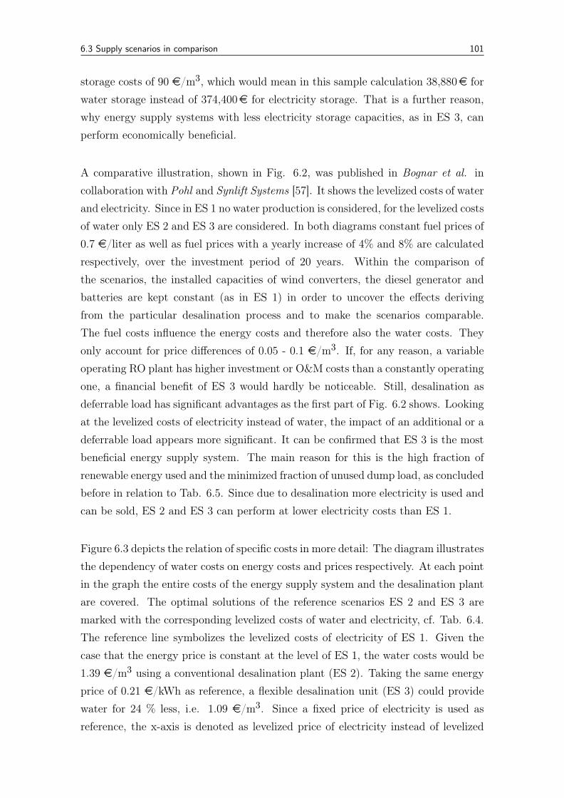
6.3 Supply scenarios in comparison 101
storage costs of 90 e/m3, which would mean in this sample calculation 38,880e forwater storage instead of 374,400e for electricity storage. That is a further reason,why energy supply systems with less electricity storage capacities, as in ES 3, canperform economically beneficial.
A comparative illustration, shown in Fig. 6.2, was published in Bognar et al. incollaboration with Pohl and Synlift Systems [57]. It shows the levelized costs of waterand electricity. Since in ES 1 no water production is considered, for the levelized costsof water only ES 2 and ES 3 are considered. In both diagrams constant fuel prices of0.7 e/liter as well as fuel prices with a yearly increase of 4% and 8% are calculatedrespectively, over the investment period of 20 years. Within the comparison ofthe scenarios, the installed capacities of wind converters, the diesel generator andbatteries are kept constant (as in ES 1) in order to uncover the effects derivingfrom the particular desalination process and to make the scenarios comparable.The fuel costs influence the energy costs and therefore also the water costs. Theyonly account for price differences of 0.05 - 0.1 e/m3. If, for any reason, a variableoperating RO plant has higher investment or O&M costs than a constantly operatingone, a financial benefit of ES 3 would hardly be noticeable. Still, desalination asdeferrable load has significant advantages as the first part of Fig. 6.2 shows. Lookingat the levelized costs of electricity instead of water, the impact of an additional or adeferrable load appears more significant. It can be confirmed that ES 3 is the mostbeneficial energy supply system. The main reason for this is the high fraction ofrenewable energy used and the minimized fraction of unused dump load, as concludedbefore in relation to Tab. 6.5. Since due to desalination more electricity is used andcan be sold, ES 2 and ES 3 can perform at lower electricity costs than ES 1.
Figure 6.3 depicts the relation of specific costs in more detail: The diagram illustratesthe dependency of water costs on energy costs and prices respectively. At each pointin the graph the entire costs of the energy supply system and the desalination plantare covered. The optimal solutions of the reference scenarios ES 2 and ES 3 aremarked with the corresponding levelized costs of water and electricity, cf. Tab. 6.4.The reference line symbolizes the levelized costs of electricity of ES 1. Given thecase that the energy price is constant at the level of ES 1, the water costs would be1.39 e/m3 using a conventional desalination plant (ES 2). Taking the same energyprice of 0.21 e/kWh as reference, a flexible desalination unit (ES 3) could providewater for 24 % less, i.e. 1.09 e/m3. Since a fixed price of electricity is used asreference, the x-axis is denoted as levelized price of electricity instead of levelized
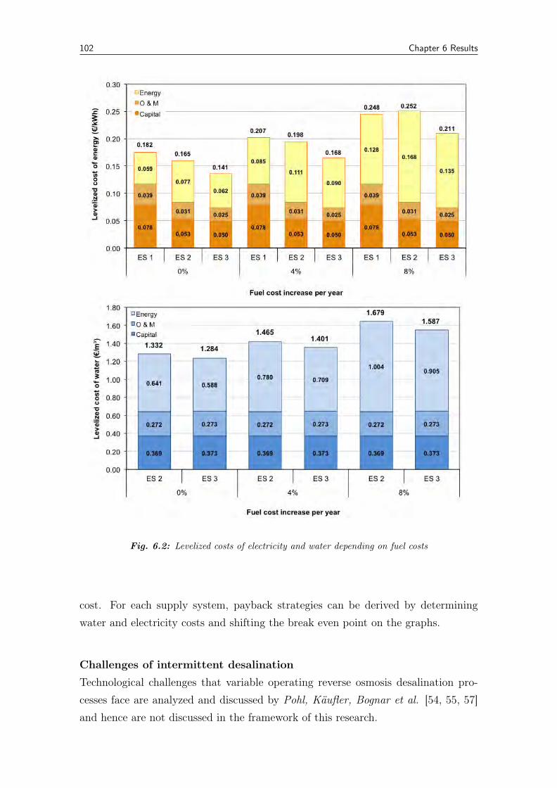
102 Chapter 6 Results
Fig. 6.2: Levelized costs of electricity and water depending on fuel costs
cost. For each supply system, payback strategies can be derived by determiningwater and electricity costs and shifting the break even point on the graphs.
Challenges of intermittent desalination
Technological challenges that variable operating reverse osmosis desalination pro-cesses face are analyzed and discussed by Pohl, Käufler, Bognar et al. [54, 55, 57]and hence are not discussed in the framework of this research.
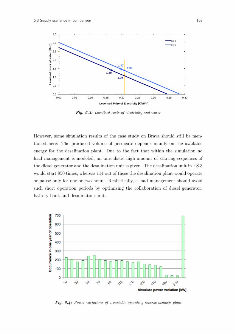
6.3 Supply scenarios in comparison 103
1.40 1.09
1.47 1.39
0.0
0.5
1.0
1.5
2.0
2.5
3.0
3.5
0.00 0.05 0.10 0.15 0.20 0.25 0.30 0.35 0.40
Leve
lised
cos
ts o
f wat
er [€
/m3 ]
Levelised Prize of Electricity [€/kWh]
ES 3
ES 2
Fig. 6.3: Levelised costs of electricity and water
However, some simulation results of the case study on Brava should still be men-tioned here: The produced volume of permeate depends mainly on the availableenergy for the desalination plant. Due to the fact that within the simulation noload management is modeled, an unrealistic high amount of starting sequences ofthe diesel generator and the desalination unit is given. The desalination unit in ES 3would start 950 times, whereas 114 out of these the desalination plant would operateor pause only for one or two hours. Realistically, a load management should avoidsuch short operation periods by optimizing the collaboration of diesel generator,battery bank and desalination unit.
Fig. 6.4: Power variations of a variable operating reverse osmosis plant
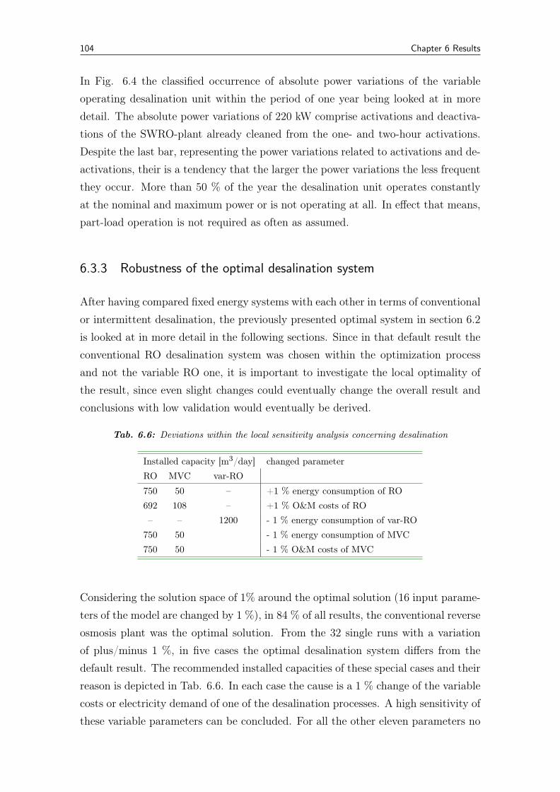
104 Chapter 6 Results
In Fig. 6.4 the classified occurrence of absolute power variations of the variableoperating desalination unit within the period of one year being looked at in moredetail. The absolute power variations of 220 kW comprise activations and deactiva-tions of the SWRO-plant already cleaned from the one- and two-hour activations.Despite the last bar, representing the power variations related to activations and de-activations, their is a tendency that the larger the power variations the less frequentthey occur. More than 50 % of the year the desalination unit operates constantlyat the nominal and maximum power or is not operating at all. In effect that means,part-load operation is not required as often as assumed.
6.3.3 Robustness of the optimal desalination system
After having compared fixed energy systems with each other in terms of conventionalor intermittent desalination, the previously presented optimal system in section 6.2is looked at in more detail in the following sections. Since in that default result theconventional RO desalination system was chosen within the optimization processand not the variable RO one, it is important to investigate the local optimality ofthe result, since even slight changes could eventually change the overall result andconclusions with low validation would eventually be derived.
Tab. 6.6: Deviations within the local sensitivity analysis concerning desalination
Installed capacity [m3/day] changed parameterRO MVC var-RO
750 50 – +1 % energy consumption of RO692 108 – +1 % O&M costs of RO– – 1200 - 1 % energy consumption of var-RO750 50 - 1 % energy consumption of MVC750 50 - 1 % O&M costs of MVC
Considering the solution space of 1% around the optimal solution (16 input parame-ters of the model are changed by 1 %), in 84 % of all results, the conventional reverseosmosis plant was the optimal solution. From the 32 single runs with a variationof plus/minus 1 %, in five cases the optimal desalination system differs from thedefault result. The recommended installed capacities of these special cases and theirreason is depicted in Tab. 6.6. In each case the cause is a 1 % change of the variablecosts or electricity demand of one of the desalination processes. A high sensitivity ofthese variable parameters can be concluded. For all the other eleven parameters no
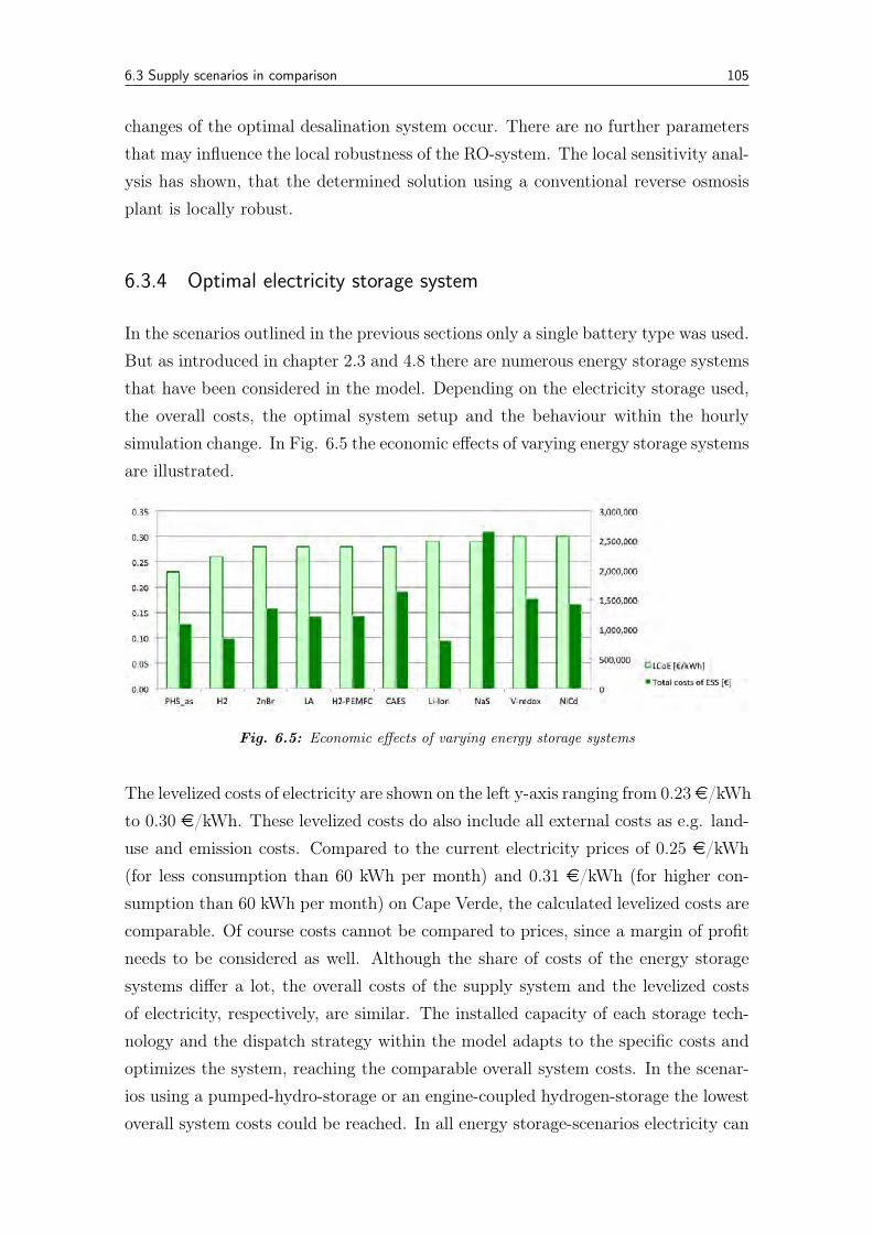
6.3 Supply scenarios in comparison 105
changes of the optimal desalination system occur. There are no further parametersthat may influence the local robustness of the RO-system. The local sensitivity anal-ysis has shown, that the determined solution using a conventional reverse osmosisplant is locally robust.
6.3.4 Optimal electricity storage system
In the scenarios outlined in the previous sections only a single battery type was used.But as introduced in chapter 2.3 and 4.8 there are numerous energy storage systemsthat have been considered in the model. Depending on the electricity storage used,the overall costs, the optimal system setup and the behaviour within the hourlysimulation change. In Fig. 6.5 the economic effects of varying energy storage systemsare illustrated.
Fig. 6.5: Economic effects of varying energy storage systems
The levelized costs of electricity are shown on the left y-axis ranging from 0.23 e/kWhto 0.30 e/kWh. These levelized costs do also include all external costs as e.g. land-use and emission costs. Compared to the current electricity prices of 0.25 e/kWh(for less consumption than 60 kWh per month) and 0.31 e/kWh (for higher con-sumption than 60 kWh per month) on Cape Verde, the calculated levelized costs arecomparable. Of course costs cannot be compared to prices, since a margin of profitneeds to be considered as well. Although the share of costs of the energy storagesystems differ a lot, the overall costs of the supply system and the levelized costsof electricity, respectively, are similar. The installed capacity of each storage tech-nology and the dispatch strategy within the model adapts to the specific costs andoptimizes the system, reaching the comparable overall system costs. In the scenar-ios using a pumped-hydro-storage or an engine-coupled hydrogen-storage the lowestoverall system costs could be reached. In all energy storage-scenarios electricity can
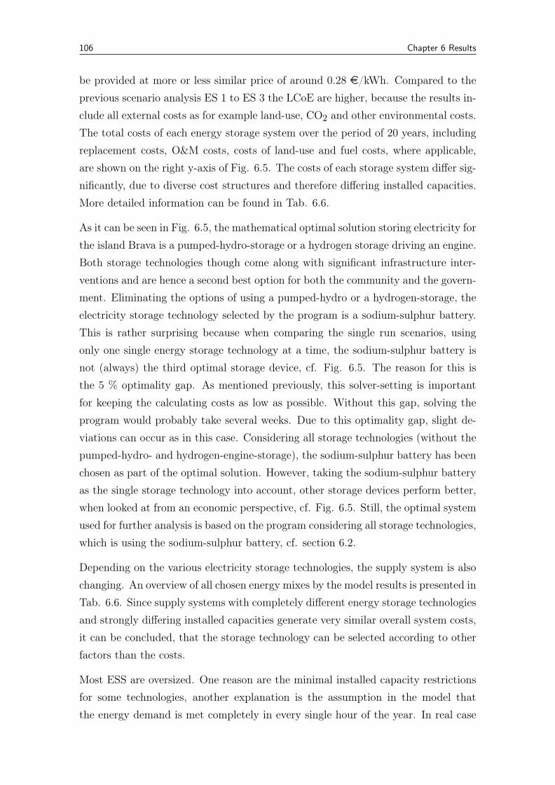
106 Chapter 6 Results
be provided at more or less similar price of around 0.28 e/kWh. Compared to theprevious scenario analysis ES 1 to ES 3 the LCoE are higher, because the results in-clude all external costs as for example land-use, CO2 and other environmental costs.The total costs of each energy storage system over the period of 20 years, includingreplacement costs, O&M costs, costs of land-use and fuel costs, where applicable,are shown on the right y-axis of Fig. 6.5. The costs of each storage system differ sig-nificantly, due to diverse cost structures and therefore differing installed capacities.More detailed information can be found in Tab. 6.6.
As it can be seen in Fig. 6.5, the mathematical optimal solution storing electricity forthe island Brava is a pumped-hydro-storage or a hydrogen storage driving an engine.Both storage technologies though come along with significant infrastructure inter-ventions and are hence a second best option for both the community and the govern-ment. Eliminating the options of using a pumped-hydro or a hydrogen-storage, theelectricity storage technology selected by the program is a sodium-sulphur battery.This is rather surprising because when comparing the single run scenarios, usingonly one single energy storage technology at a time, the sodium-sulphur battery isnot (always) the third optimal storage device, cf. Fig. 6.5. The reason for this isthe 5 % optimality gap. As mentioned previously, this solver-setting is importantfor keeping the calculating costs as low as possible. Without this gap, solving theprogram would probably take several weeks. Due to this optimality gap, slight de-viations can occur as in this case. Considering all storage technologies (without thepumped-hydro- and hydrogen-engine-storage), the sodium-sulphur battery has beenchosen as part of the optimal solution. However, taking the sodium-sulphur batteryas the single storage technology into account, other storage devices perform better,when looked at from an economic perspective, cf. Fig. 6.5. Still, the optimal systemused for further analysis is based on the program considering all storage technologies,which is using the sodium-sulphur battery, cf. section 6.2.
Depending on the various electricity storage technologies, the supply system is alsochanging. An overview of all chosen energy mixes by the model results is presented inTab. 6.6. Since supply systems with completely different energy storage technologiesand strongly differing installed capacities generate very similar overall system costs,it can be concluded, that the storage technology can be selected according to otherfactors than the costs.
Most ESS are oversized. One reason are the minimal installed capacity restrictionsfor some technologies, another explanation is the assumption in the model thatthe energy demand is met completely in every single hour of the year. In real case
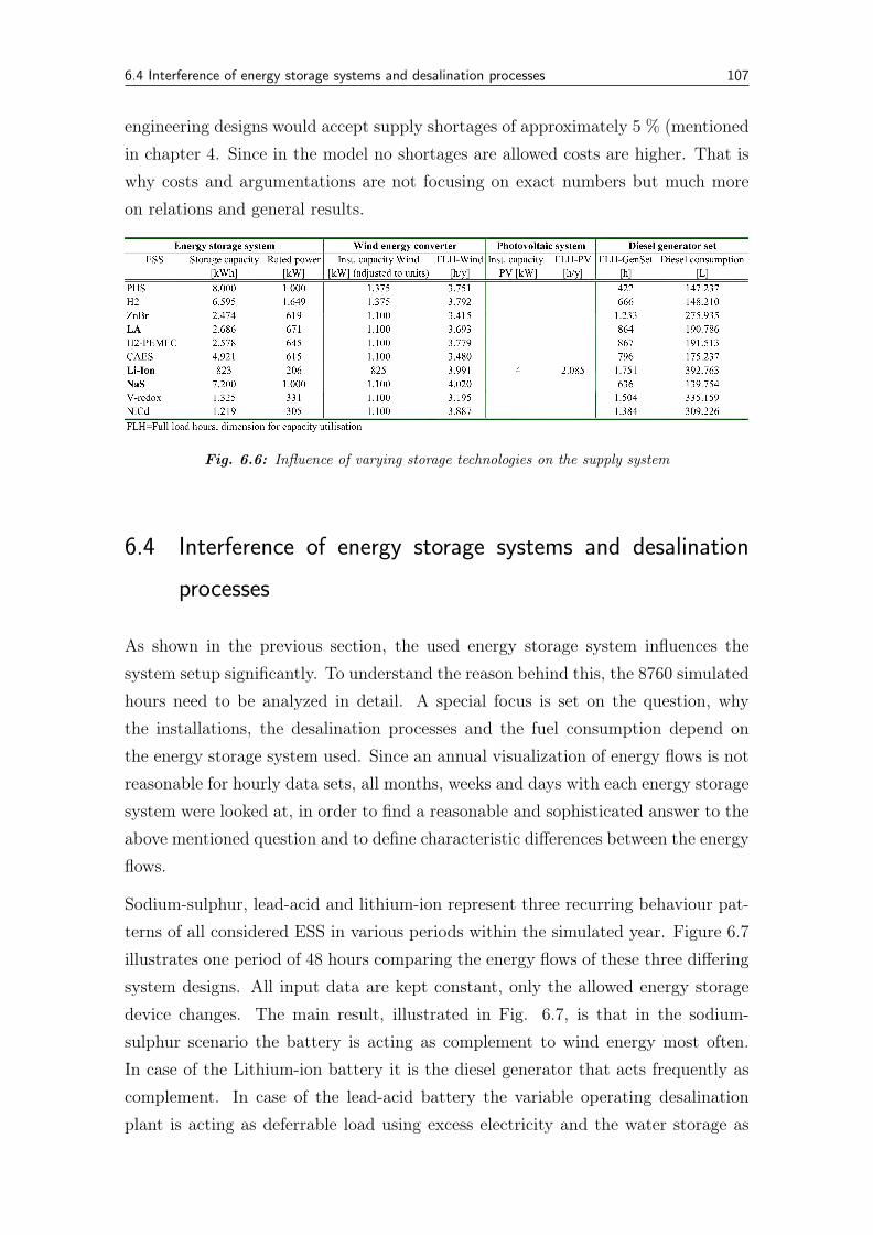
6.4 Interference of energy storage systems and desalination processes 107
engineering designs would accept supply shortages of approximately 5 % (mentionedin chapter 4. Since in the model no shortages are allowed costs are higher. That iswhy costs and argumentations are not focusing on exact numbers but much moreon relations and general results.
Fig. 6.6: Influence of varying storage technologies on the supply system
6.4 Interference of energy storage systems and desalination
processes
As shown in the previous section, the used energy storage system influences thesystem setup significantly. To understand the reason behind this, the 8760 simulatedhours need to be analyzed in detail. A special focus is set on the question, whythe installations, the desalination processes and the fuel consumption depend onthe energy storage system used. Since an annual visualization of energy flows is notreasonable for hourly data sets, all months, weeks and days with each energy storagesystem were looked at, in order to find a reasonable and sophisticated answer to theabove mentioned question and to define characteristic differences between the energyflows.
Sodium-sulphur, lead-acid and lithium-ion represent three recurring behaviour pat-terns of all considered ESS in various periods within the simulated year. Figure 6.7illustrates one period of 48 hours comparing the energy flows of these three differingsystem designs. All input data are kept constant, only the allowed energy storagedevice changes. The main result, illustrated in Fig. 6.7, is that in the sodium-sulphur scenario the battery is acting as complement to wind energy most often.In case of the Lithium-ion battery it is the diesel generator that acts frequently ascomplement. In case of the lead-acid battery the variable operating desalinationplant is acting as deferrable load using excess electricity and the water storage as
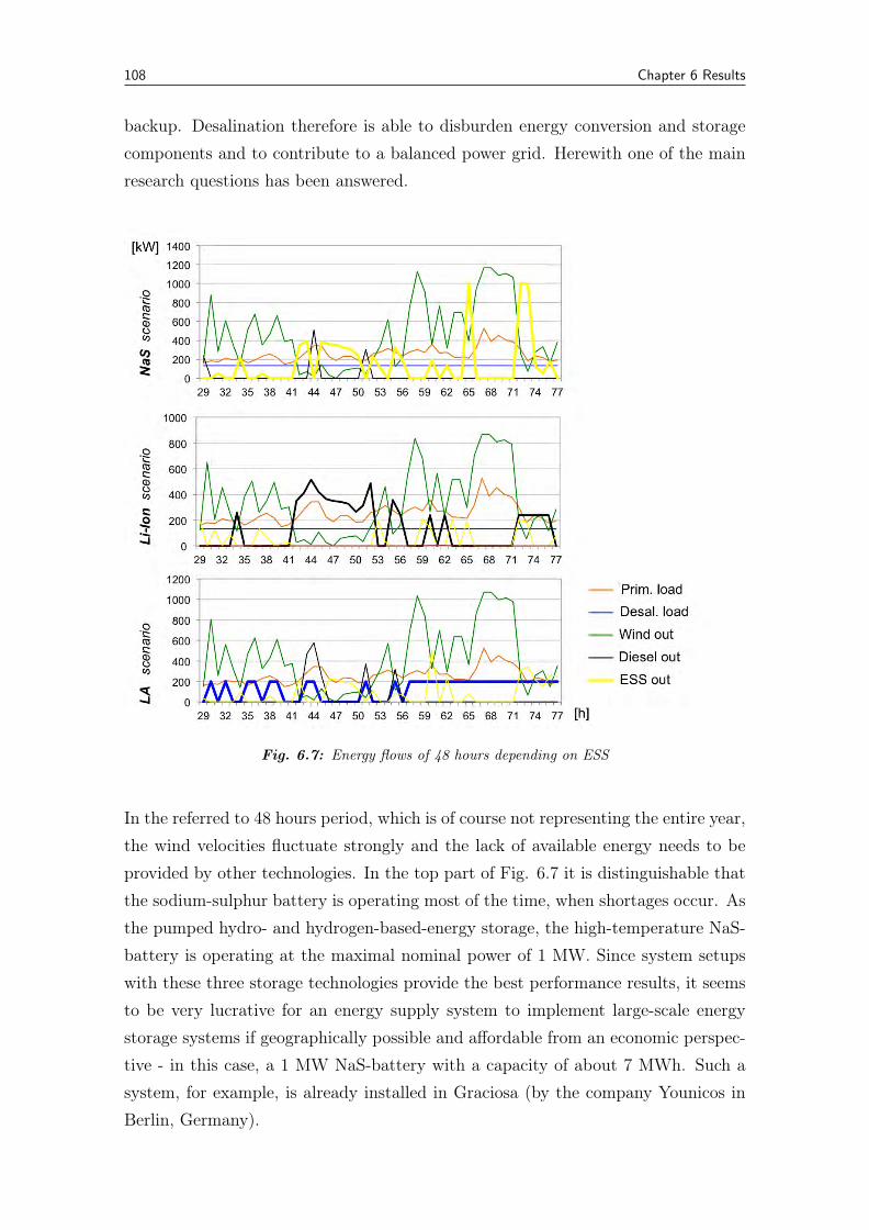
108 Chapter 6 Results
backup. Desalination therefore is able to disburden energy conversion and storagecomponents and to contribute to a balanced power grid. Herewith one of the mainresearch questions has been answered.
Fig. 6.7: Energy flows of 48 hours depending on ESS
In the referred to 48 hours period, which is of course not representing the entire year,the wind velocities fluctuate strongly and the lack of available energy needs to beprovided by other technologies. In the top part of Fig. 6.7 it is distinguishable thatthe sodium-sulphur battery is operating most of the time, when shortages occur. Asthe pumped hydro- and hydrogen-based-energy storage, the high-temperature NaS-battery is operating at the maximal nominal power of 1 MW. Since system setupswith these three storage technologies provide the best performance results, it seemsto be very lucrative for an energy supply system to implement large-scale energystorage systems if geographically possible and affordable from an economic perspec-tive - in this case, a 1 MW NaS-battery with a capacity of about 7 MWh. Such asystem, for example, is already installed in Graciosa (by the company Younicos inBerlin, Germany).
6.4 Interference of energy storage systems and desalination processes 109
The middle chart of Fig. 6.7 is showing the energy flows of the system using alithium-ion battery. Probably due to higher investment costs the installed capacityof this ESS is kept low. With 206 kW it is the smallest energy storage system,followed by the nickel-cadmium and vanadium-redox-flow battery. Most dispatchand activations have to be covered by the diesel engine, what increases the fuelconsumption and lowers its capacity factor. In this system a photovoltaic system isintegrated with a peak nominal power of 4 kW. Although its capacity is very low andthe technology is hardly contributing to the supply, it is still stabilizing the system,keeping it flexible and robust in periods of fluctuation.
In the bottom part of Fig. 6.7 the system using a lead-acid battery is shown. Herethe variable operating desalination unit is chosen within the optimization process.The battery has an installed capacity of 671 kW. Although the diesel generator isemployed more frequently than in the NaS-system, the main energetic adjustmentsare carried out by the variable operating desalination plant. Storage capacity andfuel consumption can be kept low by shifting the demand to periods when renewableexcess electricity is available. Additional to the cost-effectiveness shown in previoussections, the technological advantages of desalination as deferrable load can also beproven by investigating energy flows in hourly resolution. The energy flows withenergy storage systems as the zinc-bromine battery, the hydrogen-fuel cell and thecompressed-air-energy storage are mainly behaving as the LA-scenario with slightlyvarying characteristics.
110 Chapter 6 Results
6.5 Approach and results of a global sensitivity analysis
The motivation behind the global sensitivity analysis is to determine those factorsthat influence the respective model the most and subsequently to distinguish themfrom factors that are negligible. Contrary to a local sensitivity analysis during thisexperiment type the entire space is considered, in which factors may vary. What isnot addressed in the sensitivity analysis is the impact of volatile energy resources,such as the wind velocity and solar irradiation. A short analysis addressing thisuncertainty is presented before accomplishing the global sensitivity analysis in moredetail.
6.5.1 Impact of wind velocity and solar irradiation
All results are based on the initial data inserted in the model. The potential ofrenewable energy sources, in this case the wind velocity and the solar radiation, canunderlie various error sources. Accuracy or calibration errors of the anemometer,turbulences, climatic changes, height differences between the anemometer and theinstalled wind converter, unpredictability etc. cause deviations of the wind velocitiesused in the model compared to real wind conditions. Exact measurement uncertain-ties from calibration drift, operational uncertainties, or data gaps are unknown forground site data sets. It is assumed that quality measured data on site are moreaccurate than satellite-derived values. Nevertheless, the solar radiation data used inthe model are satellite-derived with estimated uncertainties from 6 to 12 % [112].
For both, wind and solar data, a further and decisive source for inherent errors arethe static data sets for the period of a single year. Deviations from hour to hourand day to day are included but can certainly not precisely depict real life for aninvestment period of 20 years. A sensitivity analysis can help in exemplifying theimpact of initially implemented wind velocity and insolation data.
As shown in Fig. 6.8, the optimal system setup consists out of a wind-diesel-system.The figure clarifies that for the given case the wind speed has a higher impacton the supply system than the solar irradiation. Since the measured average solarirradiation is about 6.3 kWh/m2/day and the average wind velocity 7.3 m/s (markedin Fig. 6.8), the reliability of the model output is high, even if the assumed solarand wind potentials were inaccurate. At an insulation of about 7 kWh/m2/day andan average wind velocity of under 6 m/s, the integration of photovoltaics would
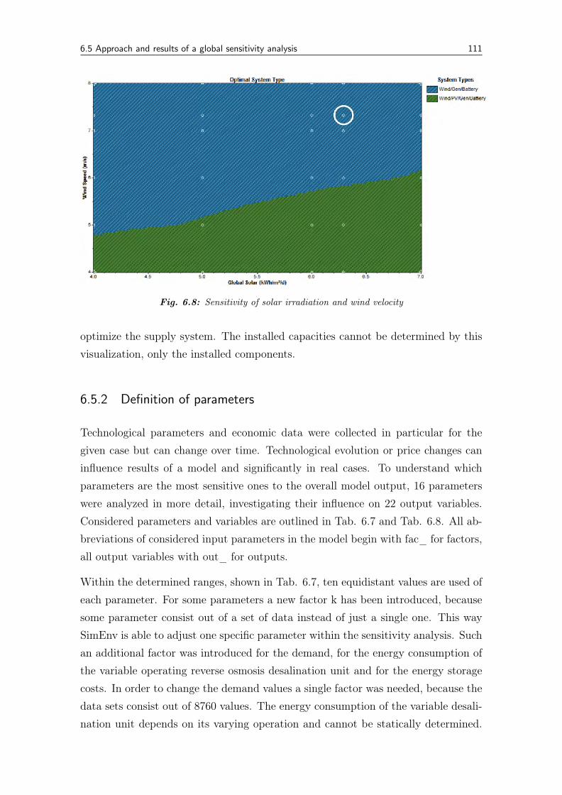
6.5 Approach and results of a global sensitivity analysis 111
Fig. 6.8: Sensitivity of solar irradiation and wind velocity
optimize the supply system. The installed capacities cannot be determined by thisvisualization, only the installed components.
6.5.2 Definition of parameters
Technological parameters and economic data were collected in particular for thegiven case but can change over time. Technological evolution or price changes caninfluence results of a model and significantly in real cases. To understand whichparameters are the most sensitive ones to the overall model output, 16 parameterswere analyzed in more detail, investigating their influence on 22 output variables.Considered parameters and variables are outlined in Tab. 6.7 and Tab. 6.8. All ab-breviations of considered input parameters in the model begin with fac_ for factors,all output variables with out_ for outputs.
Within the determined ranges, shown in Tab. 6.7, ten equidistant values are used ofeach parameter. For some parameters a new factor k has been introduced, becausesome parameter consist out of a set of data instead of just a single one. This waySimEnv is able to adjust one specific parameter within the sensitivity analysis. Suchan additional factor was introduced for the demand, for the energy consumption ofthe variable operating reverse osmosis desalination unit and for the energy storagecosts. In order to change the demand values a single factor was needed, because thedata sets consist out of 8760 values. The energy consumption of the variable desali-nation unit depends on its varying operation and cannot be statically determined.
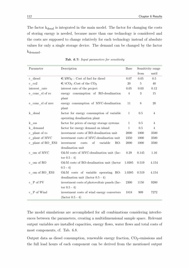
112 Chapter 6 Results
The factor kdesal is integrated in the main model. The factor for changing the costsof storing energy is needed, because more than one technology is considered andthe costs are supposed to change relatively for each technology instead of absolutevalues for only a single storage device. The demand can be changed by the factorkdemand.
Tab. 6.7: Input parameters for sensitivity
Parameter Description Base Sensitivity rangefrom until
c_diesel e/kWhf : Cost of fuel for diesel 0.07 0.05 0.5c_co2 e/tCO2 :Cost of the CO2 20 5 40interest_rate interest rate of the project 0.05 0.03 0.12e_cons_el of ro energy consumption of RO-desalination
plant4 3 15
e_cons_el of mvc energy consumption of MVC-desalinationplant
11 8 20
k_desal factor for energy consumption of variableoperating desalination plant
1 0.5 4
k_ess factor for prices of energy storage systems 1 0.5 4k_demand factor for energy demand on island 1 0.5 4c_plant of ro investment costs of RO-desalination unit 2000 1000 3500c_plant of MVC investment costs of MVC-desalination unit 2350 1000 3500c_plant of RO_ES3 investment costs of variable RO-
desalination unit2000 1000 3500
c_om of MVC O&M costs of MVC-desalination unit (fac-tor 0.5 - 4)
0.29 0.145 1.16
c_om of RO O&M costs of RO-desalination unit (factor0.5 - 4)
1.0385 0.519 4.154
c_om of RO_ES3 O&M costs of variable operating RO-desalination unit (factor 0.5 - 4)
1.0385 0.519 4.154
c_P of PV investment costs of photovoltaic panels (fac-tor 0.5 - 4)
2300 1150 9200
c_P of Wind investment costs of wind energy converters(factor 0.5 - 4)
1818 909 7272
The model simulations are accomplished for all combinations considering interfer-ences between the parameters, creating a multidimensional sample space. Relevantoutput variables are installed capacities, energy flows, water flows and total costs ofmost components, cf. Tab. 6.8.
Output data as diesel consumption, renewable energy fraction, CO2-emissions andthe full load hours of each component can be derived from the mentioned output
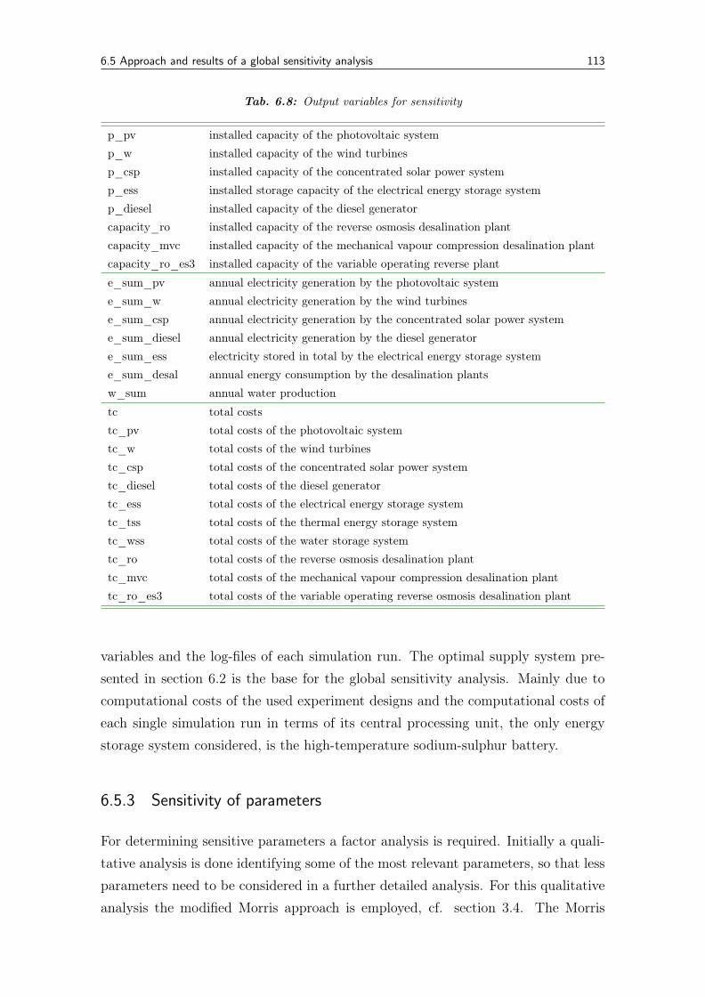
6.5 Approach and results of a global sensitivity analysis 113
Tab. 6.8: Output variables for sensitivity
p_pv installed capacity of the photovoltaic systemp_w installed capacity of the wind turbinesp_csp installed capacity of the concentrated solar power systemp_ess installed storage capacity of the electrical energy storage systemp_diesel installed capacity of the diesel generatorcapacity_ro installed capacity of the reverse osmosis desalination plantcapacity_mvc installed capacity of the mechanical vapour compression desalination plantcapacity_ro_es3 installed capacity of the variable operating reverse plant
e_sum_pv annual electricity generation by the photovoltaic systeme_sum_w annual electricity generation by the wind turbinese_sum_csp annual electricity generation by the concentrated solar power systeme_sum_diesel annual electricity generation by the diesel generatore_sum_ess electricity stored in total by the electrical energy storage systeme_sum_desal annual energy consumption by the desalination plantsw_sum annual water production
tc total coststc_pv total costs of the photovoltaic systemtc_w total costs of the wind turbinestc_csp total costs of the concentrated solar power systemtc_diesel total costs of the diesel generatortc_ess total costs of the electrical energy storage systemtc_tss total costs of the thermal energy storage systemtc_wss total costs of the water storage systemtc_ro total costs of the reverse osmosis desalination planttc_mvc total costs of the mechanical vapour compression desalination planttc_ro_es3 total costs of the variable operating reverse osmosis desalination plant
variables and the log-files of each simulation run. The optimal supply system pre-sented in section 6.2 is the base for the global sensitivity analysis. Mainly due tocomputational costs of the used experiment designs and the computational costs ofeach single simulation run in terms of its central processing unit, the only energystorage system considered, is the high-temperature sodium-sulphur battery.
6.5.3 Sensitivity of parameters
For determining sensitive parameters a factor analysis is required. Initially a quali-tative analysis is done identifying some of the most relevant parameters, so that lessparameters need to be considered in a further detailed analysis. For this qualitativeanalysis the modified Morris approach is employed, cf. section 3.4. The Morris
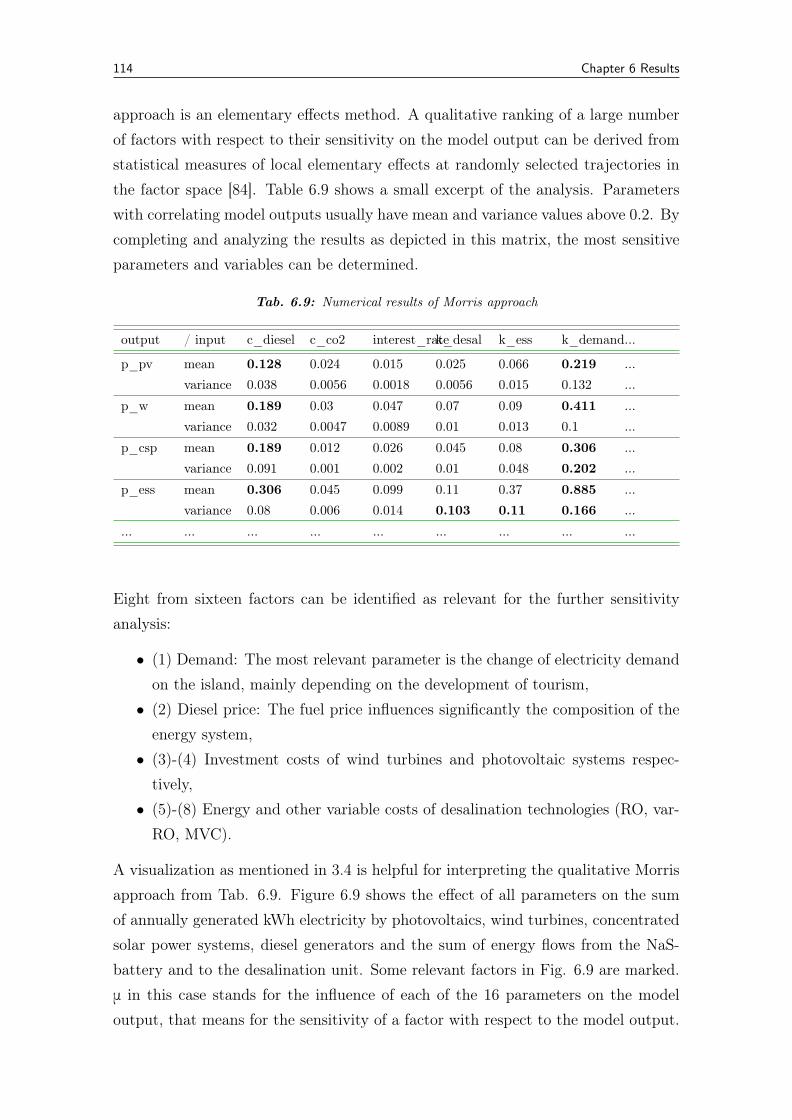
114 Chapter 6 Results
approach is an elementary effects method. A qualitative ranking of a large numberof factors with respect to their sensitivity on the model output can be derived fromstatistical measures of local elementary effects at randomly selected trajectories inthe factor space [84]. Table 6.9 shows a small excerpt of the analysis. Parameterswith correlating model outputs usually have mean and variance values above 0.2. Bycompleting and analyzing the results as depicted in this matrix, the most sensitiveparameters and variables can be determined.
Tab. 6.9: Numerical results of Morris approach
output / input c_diesel c_co2 interest_ratek_desal k_ess k_demand...
p_pv mean 0.128 0.024 0.015 0.025 0.066 0.219 ...variance 0.038 0.0056 0.0018 0.0056 0.015 0.132 ...
p_w mean 0.189 0.03 0.047 0.07 0.09 0.411 ...variance 0.032 0.0047 0.0089 0.01 0.013 0.1 ...
p_csp mean 0.189 0.012 0.026 0.045 0.08 0.306 ...variance 0.091 0.001 0.002 0.01 0.048 0.202 ...
p_ess mean 0.306 0.045 0.099 0.11 0.37 0.885 ...variance 0.08 0.006 0.014 0.103 0.11 0.166 ...
... ... ... ... ... ... ... ... ...
Eight from sixteen factors can be identified as relevant for the further sensitivityanalysis:
• (1) Demand: The most relevant parameter is the change of electricity demandon the island, mainly depending on the development of tourism,• (2) Diesel price: The fuel price influences significantly the composition of the
energy system,• (3)-(4) Investment costs of wind turbines and photovoltaic systems respec-
tively,• (5)-(8) Energy and other variable costs of desalination technologies (RO, var-
RO, MVC).
A visualization as mentioned in 3.4 is helpful for interpreting the qualitative Morrisapproach from Tab. 6.9. Figure 6.9 shows the effect of all parameters on the sumof annually generated kWh electricity by photovoltaics, wind turbines, concentratedsolar power systems, diesel generators and the sum of energy flows from the NaS-battery and to the desalination unit. Some relevant factors in Fig. 6.9 are marked.μ in this case stands for the influence of each of the 16 parameters on the modeloutput, that means for the sensitivity of a factor with respect to the model output.
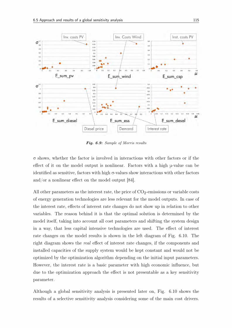
6.5 Approach and results of a global sensitivity analysis 115
Fig. 6.9: Sample of Morris results
σ shows, whether the factor is involved in interactions with other factors or if theeffect of it on the model output is nonlinear. Factors with a high μ-value can beidentified as sensitive, factors with high σ-values show interactions with other factorsand/or a nonlinear effect on the model output [84].
All other parameters as the interest rate, the price of CO2-emissions or variable costsof energy generation technologies are less relevant for the model outputs. In case ofthe interest rate, effects of interest rate changes do not show up in relation to othervariables. The reason behind it is that the optimal solution is determined by themodel itself, taking into account all cost parameters and shifting the system designin a way, that less capital intensive technologies are used. The effect of interestrate changes on the model results is shown in the left diagram of Fig. 6.10. Theright diagram shows the real effect of interest rate changes, if the components andinstalled capacities of the supply system would be kept constant and would not beoptimized by the optimization algorithm depending on the initial input parameters.However, the interest rate is a basic parameter with high economic influence, butdue to the optimization approach the effect is not presentable as a key sensitivityparameter.
Although a global sensitivity analysis is presented later on, Fig. 6.10 shows theresults of a selective sensitivity analysis considering some of the main cost drivers.
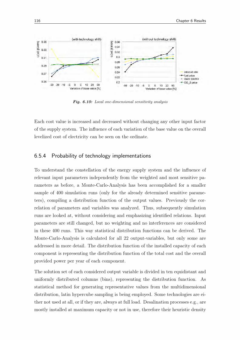
116 Chapter 6 Results
Fig. 6.10: Local one-dimensional sensitivity analysis
Each cost value is increased and decreased without changing any other input factorof the supply system. The influence of each variation of the base value on the overalllevelized cost of electricity can be seen on the ordinate.
6.5.4 Probability of technology implementations
To understand the constellation of the energy supply system and the influence ofrelevant input parameters independently from the weighted and most sensitive pa-rameters as before, a Monte-Carlo-Analysis has been accomplished for a smallersample of 400 simulation runs (only for the already determined sensitive parame-ters), compiling a distribution function of the output values. Previously the cor-relation of parameters and variables was analyzed. Thus, subsequently simulationruns are looked at, without considering and emphasizing identified relations. Inputparameters are still changed, but no weighting and no interferences are consideredin these 400 runs. This way statistical distribution functions can be derived. TheMonte-Carlo-Analysis is calculated for all 22 output-variables, but only some areaddressed in more detail. The distribution function of the installed capacity of eachcomponent is representing the distribution function of the total cost and the overallprovided power per year of each component.
The solution set of each considered output variable is divided in ten equidistant anduniformly distributed columns (bins), representing the distribution function. Asstatistical method for generating representative values from the multidimensionaldistribution, latin hypercube sampling is being employed. Some technologies are ei-ther not used at all, or if they are, always at full load. Desalination processes e.g., aremostly installed at maximum capacity or not in use, therefore their heuristic density
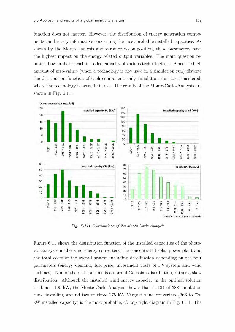
6.5 Approach and results of a global sensitivity analysis 117
function does not matter. However, the distribution of energy generation compo-nents can be very informative concerning the most probable installed capacities. Asshown by the Morris analysis and variance decomposition, these parameters havethe highest impact on the energy related output variables. The main question re-mains, how probable each installed capacity of various technologies is. Since the highamount of zero-values (when a technology is not used in a simulation run) distortsthe distribution function of each component, only simulation runs are considered,where the technology is actually in use. The results of the Monte-Carlo-Analysis areshown in Fig. 6.11.
Fig. 6.11: Distributions of the Monte Carlo Analysis
Figure 6.11 shows the distribution function of the installed capacities of the photo-voltaic system, the wind energy converters, the concentrated solar power plant andthe total costs of the overall system including desalination depending on the fourparameters (energy demand, fuel-price, investment costs of PV-system and windturbines). Non of the distributions is a normal Gaussian distribution, rather a skewdistribution. Although the installed wind energy capacity in the optimal solutionis about 1100 kW, the Monte-Carlo-Analysis shows, that in 134 of 388 simulationruns, installing around two or three 275 kW Vergnet wind converters (366 to 730kW installed capacity) is the most probable, cf. top right diagram in Fig. 6.11. The
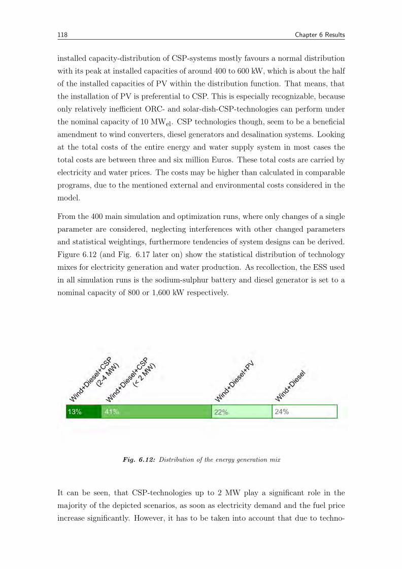
118 Chapter 6 Results
installed capacity-distribution of CSP-systems mostly favours a normal distributionwith its peak at installed capacities of around 400 to 600 kW, which is about the halfof the installed capacities of PV within the distribution function. That means, thatthe installation of PV is preferential to CSP. This is especially recognizable, becauseonly relatively inefficient ORC- and solar-dish-CSP-technologies can perform underthe nominal capacity of 10 MWel. CSP technologies though, seem to be a beneficialamendment to wind converters, diesel generators and desalination systems. Lookingat the total costs of the entire energy and water supply system in most cases thetotal costs are between three and six million Euros. These total costs are carried byelectricity and water prices. The costs may be higher than calculated in comparableprograms, due to the mentioned external and environmental costs considered in themodel.
From the 400 main simulation and optimization runs, where only changes of a singleparameter are considered, neglecting interferences with other changed parametersand statistical weightings, furthermore tendencies of system designs can be derived.Figure 6.12 (and Fig. 6.17 later on) show the statistical distribution of technologymixes for electricity generation and water production. As recollection, the ESS usedin all simulation runs is the sodium-sulphur battery and diesel generator is set to anominal capacity of 800 or 1,600 kW respectively.
Fig. 6.12: Distribution of the energy generation mix
It can be seen, that CSP-technologies up to 2 MW play a significant role in themajority of the depicted scenarios, as soon as electricity demand and the fuel priceincrease significantly. However, it has to be taken into account that due to techno-
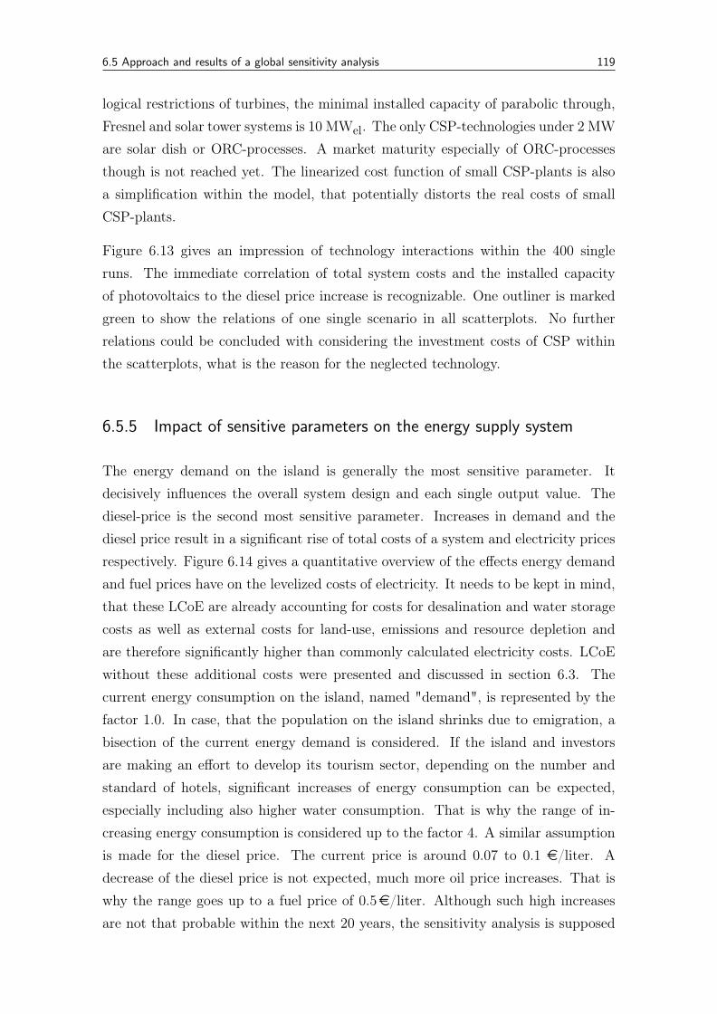
6.5 Approach and results of a global sensitivity analysis 119
logical restrictions of turbines, the minimal installed capacity of parabolic through,Fresnel and solar tower systems is 10 MWel. The only CSP-technologies under 2 MWare solar dish or ORC-processes. A market maturity especially of ORC-processesthough is not reached yet. The linearized cost function of small CSP-plants is alsoa simplification within the model, that potentially distorts the real costs of smallCSP-plants.
Figure 6.13 gives an impression of technology interactions within the 400 singleruns. The immediate correlation of total system costs and the installed capacityof photovoltaics to the diesel price increase is recognizable. One outliner is markedgreen to show the relations of one single scenario in all scatterplots. No furtherrelations could be concluded with considering the investment costs of CSP withinthe scatterplots, what is the reason for the neglected technology.
6.5.5 Impact of sensitive parameters on the energy supply system
The energy demand on the island is generally the most sensitive parameter. Itdecisively influences the overall system design and each single output value. Thediesel-price is the second most sensitive parameter. Increases in demand and thediesel price result in a significant rise of total costs of a system and electricity pricesrespectively. Figure 6.14 gives a quantitative overview of the effects energy demandand fuel prices have on the levelized costs of electricity. It needs to be kept in mind,that these LCoE are already accounting for costs for desalination and water storagecosts as well as external costs for land-use, emissions and resource depletion andare therefore significantly higher than commonly calculated electricity costs. LCoEwithout these additional costs were presented and discussed in section 6.3. Thecurrent energy consumption on the island, named "demand", is represented by thefactor 1.0. In case, that the population on the island shrinks due to emigration, abisection of the current energy demand is considered. If the island and investorsare making an effort to develop its tourism sector, depending on the number andstandard of hotels, significant increases of energy consumption can be expected,especially including also higher water consumption. That is why the range of in-creasing energy consumption is considered up to the factor 4. A similar assumptionis made for the diesel price. The current price is around 0.07 to 0.1 e/liter. Adecrease of the diesel price is not expected, much more oil price increases. That iswhy the range goes up to a fuel price of 0.5e/liter. Although such high increasesare not that probable within the next 20 years, the sensitivity analysis is supposed
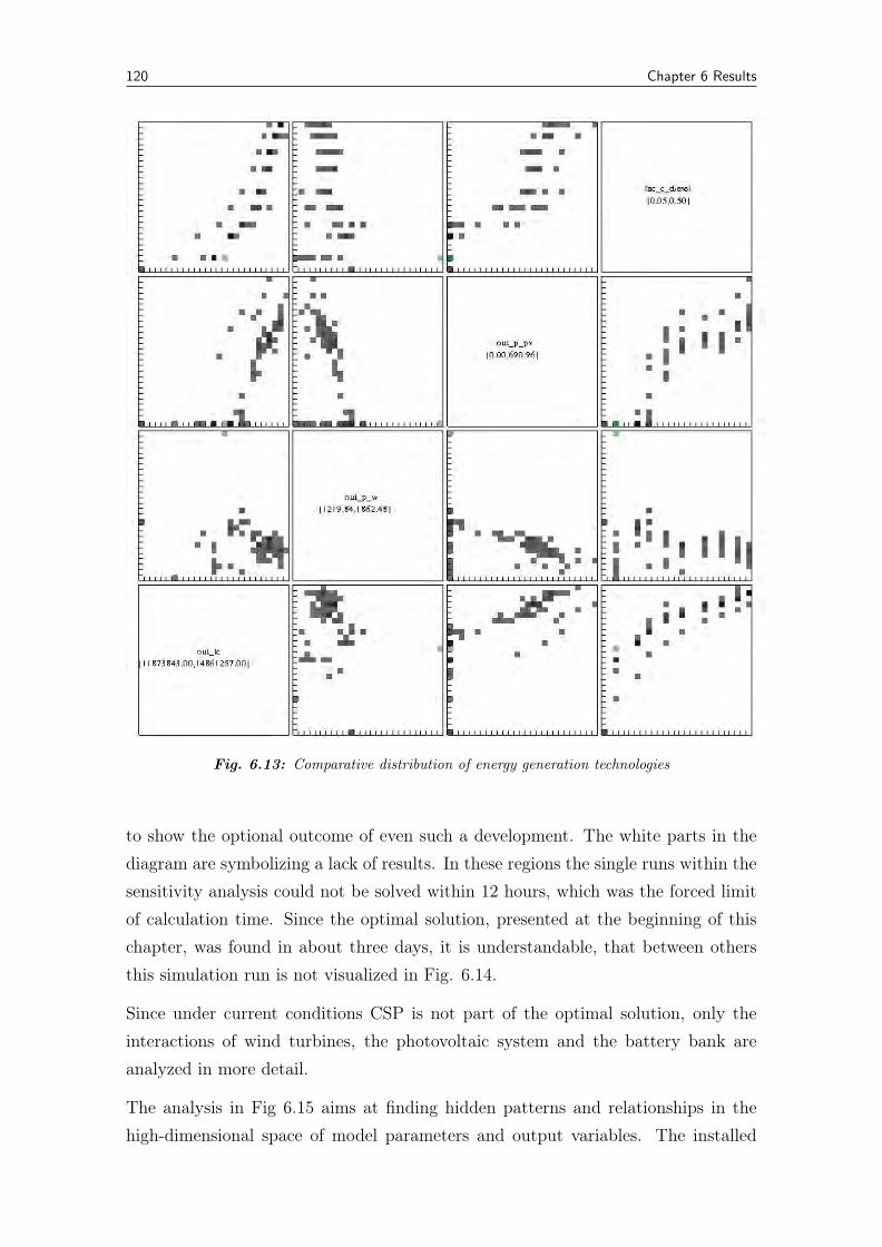
120 Chapter 6 Results
Fig. 6.13: Comparative distribution of energy generation technologies
to show the optional outcome of even such a development. The white parts in thediagram are symbolizing a lack of results. In these regions the single runs within thesensitivity analysis could not be solved within 12 hours, which was the forced limitof calculation time. Since the optimal solution, presented at the beginning of thischapter, was found in about three days, it is understandable, that between othersthis simulation run is not visualized in Fig. 6.14.
Since under current conditions CSP is not part of the optimal solution, only theinteractions of wind turbines, the photovoltaic system and the battery bank areanalyzed in more detail.
The analysis in Fig 6.15 aims at finding hidden patterns and relationships in thehigh-dimensional space of model parameters and output variables. The installed
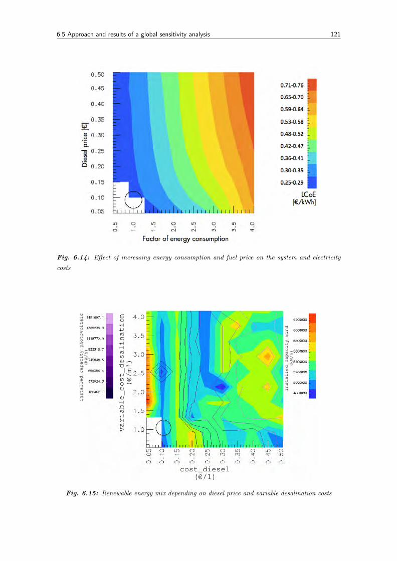
6.5 Approach and results of a global sensitivity analysis 121
Fig. 6.14: Effect of increasing energy consumption and fuel price on the system and electricitycosts
Fig. 6.15: Renewable energy mix depending on diesel price and variable desalination costs
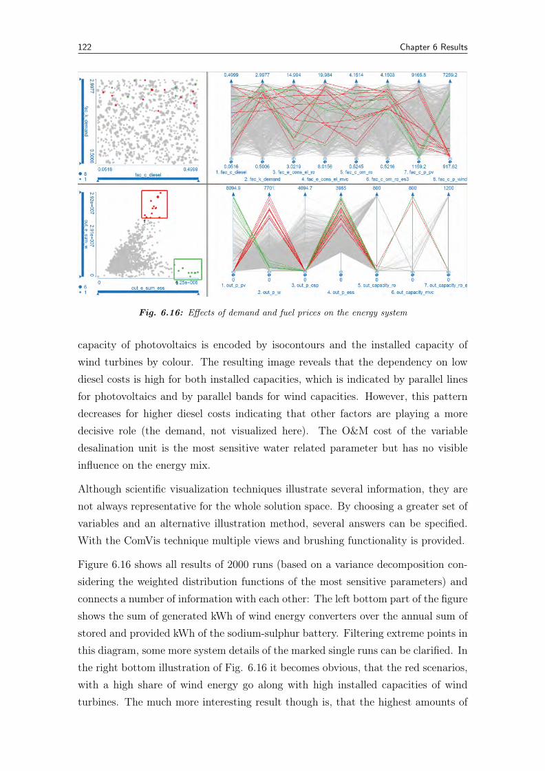
122 Chapter 6 Results
Fig. 6.16: Effects of demand and fuel prices on the energy system
capacity of photovoltaics is encoded by isocontours and the installed capacity ofwind turbines by colour. The resulting image reveals that the dependency on lowdiesel costs is high for both installed capacities, which is indicated by parallel linesfor photovoltaics and by parallel bands for wind capacities. However, this patterndecreases for higher diesel costs indicating that other factors are playing a moredecisive role (the demand, not visualized here). The O&M cost of the variabledesalination unit is the most sensitive water related parameter but has no visibleinfluence on the energy mix.
Although scientific visualization techniques illustrate several information, they arenot always representative for the whole solution space. By choosing a greater set ofvariables and an alternative illustration method, several answers can be specified.With the ComVis technique multiple views and brushing functionality is provided.
Figure 6.16 shows all results of 2000 runs (based on a variance decomposition con-sidering the weighted distribution functions of the most sensitive parameters) andconnects a number of information with each other: The left bottom part of the figureshows the sum of generated kWh of wind energy converters over the annual sum ofstored and provided kWh of the sodium-sulphur battery. Filtering extreme points inthis diagram, some more system details of the marked single runs can be clarified. Inthe right bottom illustration of Fig. 6.16 it becomes obvious, that the red scenarios,with a high share of wind energy go along with high installed capacities of windturbines. The much more interesting result though is, that the highest amounts of
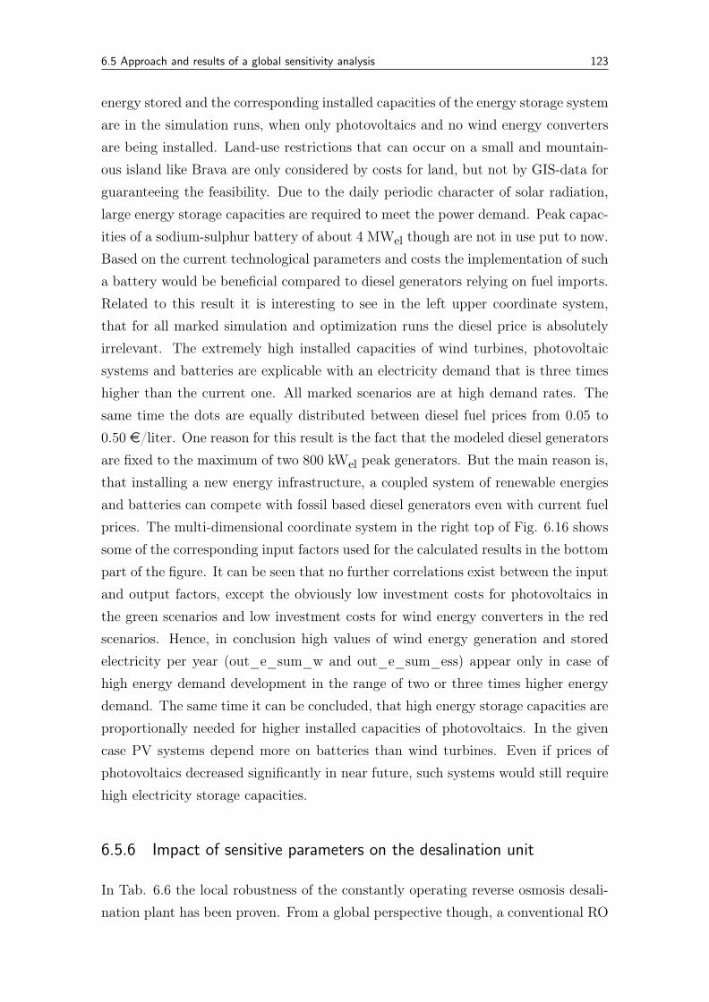
6.5 Approach and results of a global sensitivity analysis 123
energy stored and the corresponding installed capacities of the energy storage systemare in the simulation runs, when only photovoltaics and no wind energy convertersare being installed. Land-use restrictions that can occur on a small and mountain-ous island like Brava are only considered by costs for land, but not by GIS-data forguaranteeing the feasibility. Due to the daily periodic character of solar radiation,large energy storage capacities are required to meet the power demand. Peak capac-ities of a sodium-sulphur battery of about 4 MWel though are not in use put to now.Based on the current technological parameters and costs the implementation of sucha battery would be beneficial compared to diesel generators relying on fuel imports.Related to this result it is interesting to see in the left upper coordinate system,that for all marked simulation and optimization runs the diesel price is absolutelyirrelevant. The extremely high installed capacities of wind turbines, photovoltaicsystems and batteries are explicable with an electricity demand that is three timeshigher than the current one. All marked scenarios are at high demand rates. Thesame time the dots are equally distributed between diesel fuel prices from 0.05 to0.50 e/liter. One reason for this result is the fact that the modeled diesel generatorsare fixed to the maximum of two 800 kWel peak generators. But the main reason is,that installing a new energy infrastructure, a coupled system of renewable energiesand batteries can compete with fossil based diesel generators even with current fuelprices. The multi-dimensional coordinate system in the right top of Fig. 6.16 showssome of the corresponding input factors used for the calculated results in the bottompart of the figure. It can be seen that no further correlations exist between the inputand output factors, except the obviously low investment costs for photovoltaics inthe green scenarios and low investment costs for wind energy converters in the redscenarios. Hence, in conclusion high values of wind energy generation and storedelectricity per year (out_e_sum_w and out_e_sum_ess) appear only in case ofhigh energy demand development in the range of two or three times higher energydemand. The same time it can be concluded, that high energy storage capacities areproportionally needed for higher installed capacities of photovoltaics. In the givencase PV systems depend more on batteries than wind turbines. Even if prices ofphotovoltaics decreased significantly in near future, such systems would still requirehigh electricity storage capacities.
6.5.6 Impact of sensitive parameters on the desalination unit
In Tab. 6.6 the local robustness of the constantly operating reverse osmosis desali-nation plant has been proven. From a global perspective though, a conventional RO
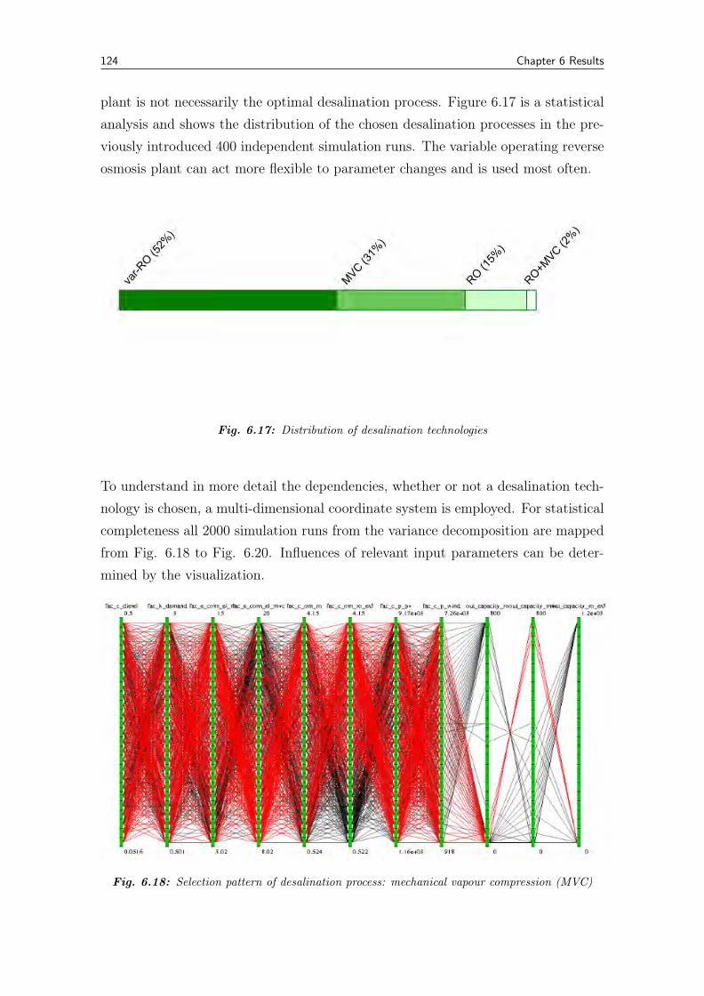
124 Chapter 6 Results
plant is not necessarily the optimal desalination process. Figure 6.17 is a statisticalanalysis and shows the distribution of the chosen desalination processes in the pre-viously introduced 400 independent simulation runs. The variable operating reverseosmosis plant can act more flexible to parameter changes and is used most often.
Fig. 6.17: Distribution of desalination technologies
To understand in more detail the dependencies, whether or not a desalination tech-nology is chosen, a multi-dimensional coordinate system is employed. For statisticalcompleteness all 2000 simulation runs from the variance decomposition are mappedfrom Fig. 6.18 to Fig. 6.20. Influences of relevant input parameters can be deter-mined by the visualization.
Fig. 6.18: Selection pattern of desalination process: mechanical vapour compression (MVC)
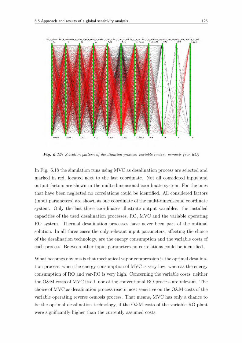
6.5 Approach and results of a global sensitivity analysis 125
Fig. 6.19: Selection pattern of desalination process: variable reverse osmosis (var-RO)
In Fig. 6.18 the simulation runs using MVC as desalination process are selected andmarked in red, located next to the last coordinate. Not all considered input andoutput factors are shown in the multi-dimensional coordinate system. For the onesthat have been neglected no correlations could be identified. All considered factors(input parameters) are shown as one coordinate of the multi-dimensional coordinatesystem. Only the last three coordinates illustrate output variables: the installedcapacities of the used desalination processes, RO, MVC and the variable operatingRO system. Thermal desalination processes have never been part of the optimalsolution. In all three cases the only relevant input parameters, affecting the choiceof the desalination technology, are the energy consumption and the variable costs ofeach process. Between other input parameters no correlations could be identified.
What becomes obvious is that mechanical vapor compression is the optimal desalina-tion process, when the energy consumption of MVC is very low, whereas the energyconsumption of RO and var-RO is very high. Concerning the variable costs, neitherthe O&M costs of MVC itself, nor of the conventional RO-process are relevant. Thechoice of MVC as desalination process reacts most sensitive on the O&M costs of thevariable operating reverse osmosis process. That means, MVC has only a chance tobe the optimal desalination technology, if the O&M costs of the variable RO-plantwere significantly higher than the currently assumed costs.
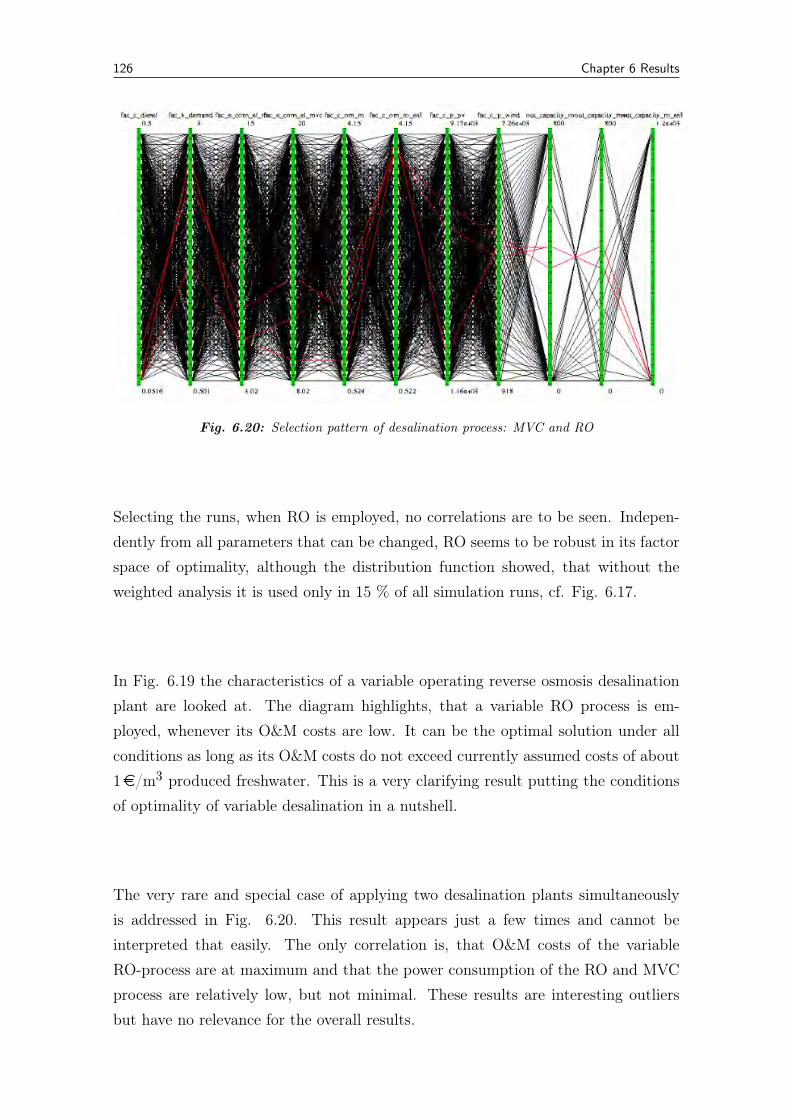
126 Chapter 6 Results
Fig. 6.20: Selection pattern of desalination process: MVC and RO
Selecting the runs, when RO is employed, no correlations are to be seen. Indepen-dently from all parameters that can be changed, RO seems to be robust in its factorspace of optimality, although the distribution function showed, that without theweighted analysis it is used only in 15 % of all simulation runs, cf. Fig. 6.17.
In Fig. 6.19 the characteristics of a variable operating reverse osmosis desalinationplant are looked at. The diagram highlights, that a variable RO process is em-ployed, whenever its O&M costs are low. It can be the optimal solution under allconditions as long as its O&M costs do not exceed currently assumed costs of about1e/m3 produced freshwater. This is a very clarifying result putting the conditionsof optimality of variable desalination in a nutshell.
The very rare and special case of applying two desalination plants simultaneouslyis addressed in Fig. 6.20. This result appears just a few times and cannot beinterpreted that easily. The only correlation is, that O&M costs of the variableRO-process are at maximum and that the power consumption of the RO and MVCprocess are relatively low, but not minimal. These results are interesting outliersbut have no relevance for the overall results.
6.6 Economic reflection: Investment strategies based on the real option approach (ROA) 127
6.6 Economic reflection: Investment strategies based on the
real option approach (ROA)
Since up to now no touristic development is planned on Brava and the main goal ofthe local government is to find ways to become more independent from fossil fuelsand to increase their share of renewable energies, the uncertainty of the future oilprice is considered by the following real option analysis. As described in the method-ology chapter 3.5, the real option analysis is an alternative economic approach forevaluating optimal supply systems considering uncertainty. The goal is to deter-mine, whether a statical optimal system still remains the optimal one, even whensensitive parameters are volatile or change significantly.
In this context a single parameter is considered separately and in more detail forguaranteeing transparency and measurability. As real option method the binomiallattice approach is chosen, without implementing it in a dynamic program, becausethis way intermediate values and decisions become visible. If the practicability canbe verified, other sensitive and uncertain parameters can be included in a dynamicprogramming approach subsequently.
Figure 6.21 shows the results of a one-dimensional sensitivity analysis consideringonly the diesel price. In some cases relevant scenarios can be derived for the binomialdecision tree approach.
Depending on various diesel price developments, for four various diesel prices optimalscenarios were identified, cf. Tab. 6.10. In all these scenarios conventional lead acidbatteries to have the highest flexibility concerning the installed storage capacity. Asanalyzed before (cf. section 6.1) the optimal energy supply system including theenergy demand of the desalination plant at current fuel prices of e0.7/liter consistsout of three 275 kW wind turbines, a small capacity of PV modules (88 kW), one800 kW diesel generator and LA batteries with a storage capacity of around 2500kWh.
Scenario BaU (Business as Usual) describes the current system with power supplyby diesel generators only. In scenario Wind1 a smaller share of wind energy isinstalled (three WECs), in Wind2 five WECs. In scenario Wind1+PV again threeWECs are implemented but also a photovoltaic system with a nominal capacity of800 kWpeak. It cannot be decided that easily, which scenario would be the mostrobust against oil price uncertainties. Each scenario is optimal for different constantfuel prices.
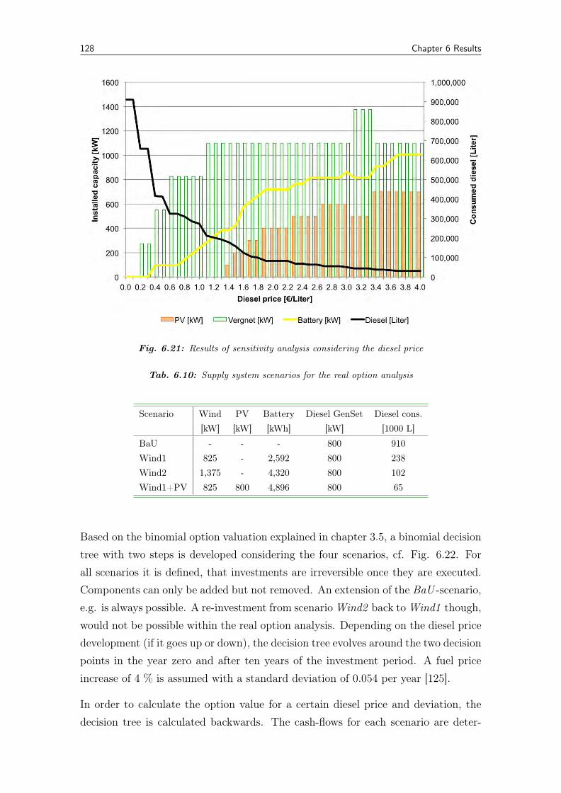
128 Chapter 6 Results
Fig. 6.21: Results of sensitivity analysis considering the diesel price
Tab. 6.10: Supply system scenarios for the real option analysis
Scenario Wind PV Battery Diesel GenSet Diesel cons.[kW] [kW] [kWh] [kW] [1000 L]
BaU - - - 800 910Wind1 825 - 2,592 800 238Wind2 1,375 - 4,320 800 102Wind1+PV 825 800 4,896 800 65
Based on the binomial option valuation explained in chapter 3.5, a binomial decisiontree with two steps is developed considering the four scenarios, cf. Fig. 6.22. Forall scenarios it is defined, that investments are irreversible once they are executed.Components can only be added but not removed. An extension of the BaU -scenario,e.g. is always possible. A re-investment from scenarioWind2 back toWind1 though,would not be possible within the real option analysis. Depending on the diesel pricedevelopment (if it goes up or down), the decision tree evolves around the two decisionpoints in the year zero and after ten years of the investment period. A fuel priceincrease of 4 % is assumed with a standard deviation of 0.054 per year [125].
In order to calculate the option value for a certain diesel price and deviation, thedecision tree is calculated backwards. The cash-flows for each scenario are deter-
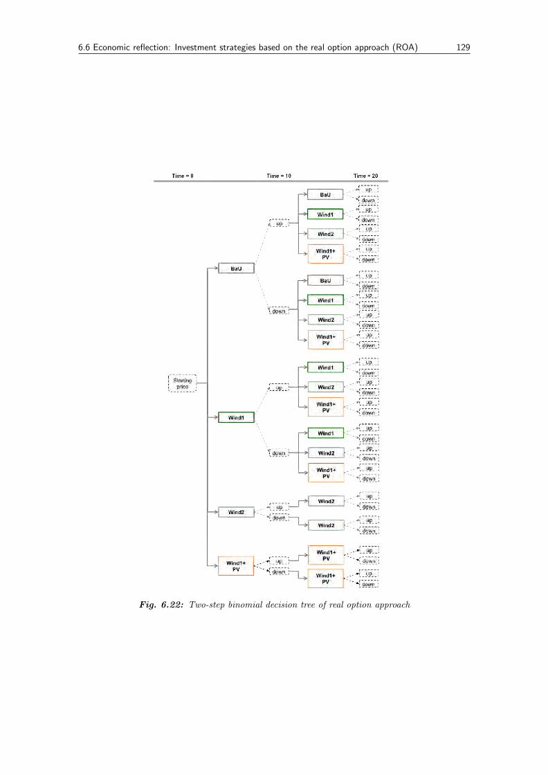
6.6 Economic reflection: Investment strategies based on the real option approach (ROA) 129
Fig. 6.22: Two-step binomial decision tree of real option approach
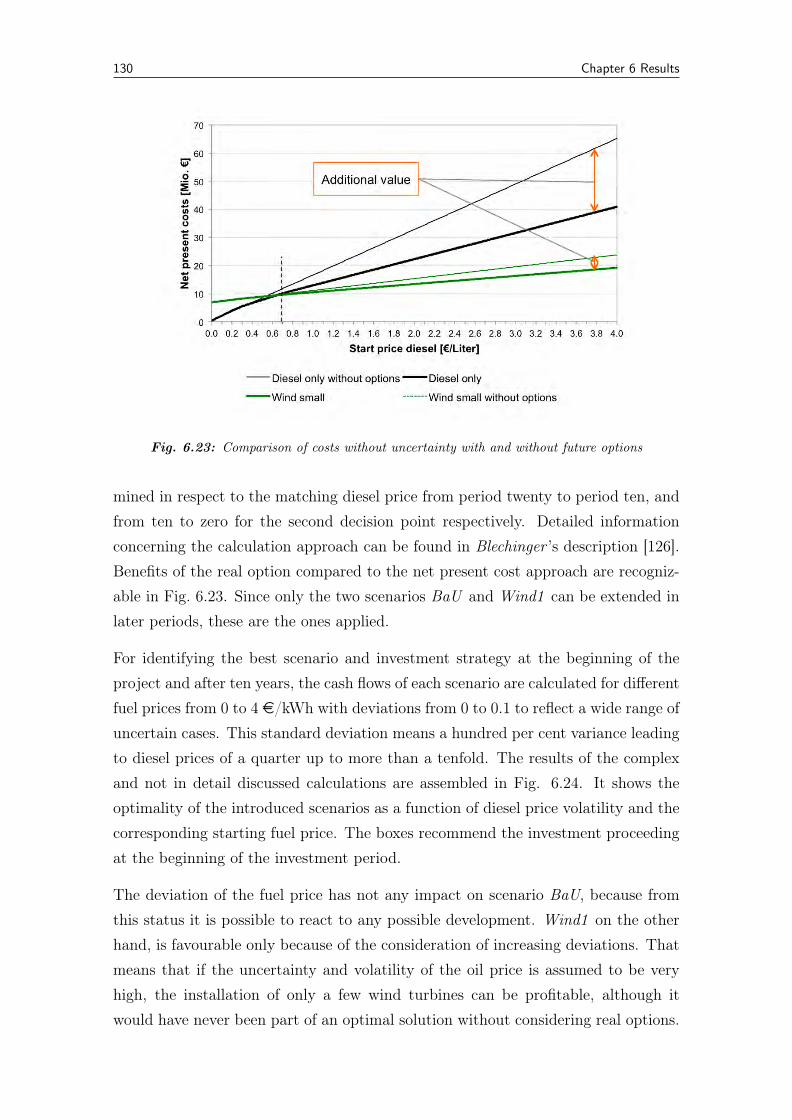
130 Chapter 6 Results
Fig. 6.23: Comparison of costs without uncertainty with and without future options
mined in respect to the matching diesel price from period twenty to period ten, andfrom ten to zero for the second decision point respectively. Detailed informationconcerning the calculation approach can be found in Blechinger ’s description [126].Benefits of the real option compared to the net present cost approach are recogniz-able in Fig. 6.23. Since only the two scenarios BaU and Wind1 can be extended inlater periods, these are the ones applied.
For identifying the best scenario and investment strategy at the beginning of theproject and after ten years, the cash flows of each scenario are calculated for differentfuel prices from 0 to 4 e/kWh with deviations from 0 to 0.1 to reflect a wide range ofuncertain cases. This standard deviation means a hundred per cent variance leadingto diesel prices of a quarter up to more than a tenfold. The results of the complexand not in detail discussed calculations are assembled in Fig. 6.24. It shows theoptimality of the introduced scenarios as a function of diesel price volatility and thecorresponding starting fuel price. The boxes recommend the investment proceedingat the beginning of the investment period.
The deviation of the fuel price has not any impact on scenario BaU, because fromthis status it is possible to react to any possible development. Wind1 on the otherhand, is favourable only because of the consideration of increasing deviations. Thatmeans that if the uncertainty and volatility of the oil price is assumed to be veryhigh, the installation of only a few wind turbines can be profitable, although itwould have never been part of an optimal solution without considering real options.
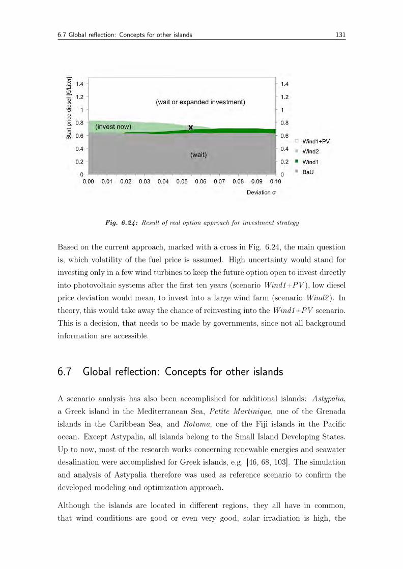
6.7 Global reflection: Concepts for other islands 131
Fig. 6.24: Result of real option approach for investment strategy
Based on the current approach, marked with a cross in Fig. 6.24, the main questionis, which volatility of the fuel price is assumed. High uncertainty would stand forinvesting only in a few wind turbines to keep the future option open to invest directlyinto photovoltaic systems after the first ten years (scenario Wind1+PV ), low dieselprice deviation would mean, to invest into a large wind farm (scenario Wind2 ). Intheory, this would take away the chance of reinvesting into the Wind1+PV scenario.This is a decision, that needs to be made by governments, since not all backgroundinformation are accessible.
6.7 Global reflection: Concepts for other islands
A scenario analysis has also been accomplished for additional islands: Astypalia,a Greek island in the Mediterranean Sea, Petite Martinique, one of the Grenadaislands in the Caribbean Sea, and Rotuma, one of the Fiji islands in the Pacificocean. Except Astypalia, all islands belong to the Small Island Developing States.Up to now, most of the research works concerning renewable energies and seawaterdesalination were accomplished for Greek islands, e.g. [46, 68, 103]. The simulationand analysis of Astypalia therefore was used as reference scenario to confirm thedeveloped modeling and optimization approach.
Although the islands are located in different regions, they all have in common,that wind conditions are good or even very good, solar irradiation is high, the
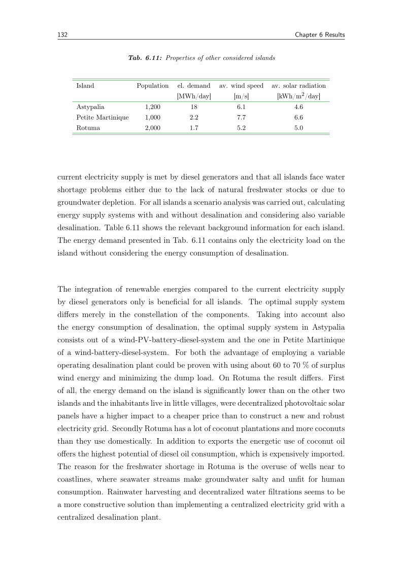
132 Chapter 6 Results
Tab. 6.11: Properties of other considered islands
Island Population el. demand av. wind speed av. solar radiation[MWh/day] [m/s] [kWh/m2/day]
Astypalia 1,200 18 6.1 4.6Petite Martinique 1,000 2.2 7.7 6.6Rotuma 2,000 1.7 5.2 5.0
current electricity supply is met by diesel generators and that all islands face watershortage problems either due to the lack of natural freshwater stocks or due togroundwater depletion. For all islands a scenario analysis was carried out, calculatingenergy supply systems with and without desalination and considering also variabledesalination. Table 6.11 shows the relevant background information for each island.The energy demand presented in Tab. 6.11 contains only the electricity load on theisland without considering the energy consumption of desalination.
The integration of renewable energies compared to the current electricity supplyby diesel generators only is beneficial for all islands. The optimal supply systemdiffers merely in the constellation of the components. Taking into account alsothe energy consumption of desalination, the optimal supply system in Astypaliaconsists out of a wind-PV-battery-diesel-system and the one in Petite Martiniqueof a wind-battery-diesel-system. For both the advantage of employing a variableoperating desalination plant could be proven with using about 60 to 70 % of surpluswind energy and minimizing the dump load. On Rotuma the result differs. Firstof all, the energy demand on the island is significantly lower than on the other twoislands and the inhabitants live in little villages, were decentralized photovoltaic solarpanels have a higher impact to a cheaper price than to construct a new and robustelectricity grid. Secondly Rotuma has a lot of coconut plantations and more coconutsthan they use domestically. In addition to exports the energetic use of coconut oiloffers the highest potential of diesel oil consumption, which is expensively imported.The reason for the freshwater shortage in Rotuma is the overuse of wells near tocoastlines, where seawater streams make groundwater salty and unfit for humanconsumption. Rainwater harvesting and decentralized water filtrations seems to bea more constructive solution than implementing a centralized electricity grid with acentralized desalination plant.

6.7 Global reflection: Concepts for other islands 133
Overall, the presented results for the Cape Verde island Brava can be confirmed byislands with comparable properties and are transferable to remote arid regions in aglobal perspective.
Chapter
7Conclusions
7.1 Summary and conclusions
Using the modeling system GAMS a model for optimizing self-sufficient energy andwater supply systems for remote regions has been developed. The central motivationof the research work has been to answer questions related to the following questions:
• How do various electricity storage technologies influence the optimal energyand water supply system?• What effect does the integration of a deferrable desalination unit have on the
system setup?• How do changes of the diesel price, the energy demand or prices of components
affect the system design?
Since no available model is able to answer these and related questions, an energysupply with integrated seawater desalination units is modeled and programmed. Themodel focuses on remote regions, where isolated island grids are in use. Basics of en-ergy engineering and water supply are introduced and the Cape Verde island Bravaidentified as case study. Hourly measured data of one year are the base for realis-tic simulation results. Energy systems considering various generation technologies,energy storages and desalination processes are calculated, compared and a sensitiv-ity analysis employed. In order to determine the robustness of a system, a globalsensitivity analysis is applied using the simulation environment SimEnv within theGAMS model.
The effects of varying desalination processes and varying energy storage systemshave been analyzed and discussed in detail. Focussing on the respective researchobjectives a number of results can be concluded:
7.1 Summary and conclusions 135
The integration of renewable energies is beneficial in considered island
grids.
The integration of renewable energy technologies to the current energy supply systemon the investigated island is beneficial from an economic as well as from an ecologicalperspective even without considering freshwater production. The optimal energysupply system (at current conditions) is a hybrid wind-diesel-battery system. In caseof increasing fuel prices and increasing energy consumption, the implementation ofphotovoltaics and concentrated solar power technologies would be beneficial, as thesensitivity analysis has shown. The current demand could be met with electricityprices of 0.21e/kWh instead of 0.31e/kWh for the investment period of twentyyears. About 1 MW wind energy capacity should be installed on the Cape Verdeisland independently from any fuel price or demand change. Depending on thedevelopment strategy of the local government, additional photovoltaic capacitiesmay be installed in case of enhancements, e.g. due to growing tourism.
The optimal energy and water supply system at current conditions is a
wind-diesel-battery system with a reverse osmosis-desalination unit.
Integrating desalination to the island grid the optimal system, cf. section 6.2, con-sists out of four 275 kW Vergnet wind turbines, a diesel generator with the capacityof 800 kWel and a sodium-sulphur battery with the peak discharge power of 1 MWand a storage capacity of 7.2 MWh. The desalination technology chosen within theoptimization process is a conventional, constantly operating reverse osmosis unitproducing 800 m3 fresh water per day with an energy consumption of 4 kWh/m3.The overall costs of the system are about 12.6 million Euros. With the assumptionof constant diesel prices electricity costs could be kept on the level of 0.16e/kWhand water costs at 1.53e/m3 for the period of twenty years.
The choice of the electricity storage system can change optimal capacities
and components.
Depending on the energy storage technology used, the installed capacities of allcomponents and the hourly dispatch behaviours change, and even PV systems canbe part of the optimal solution. The lowest overall system costs can be reached byusing pumped-hydro-storage systems or engine-coupled-hydrogen-storages. Thesetwo technologies though, are not applicable on Brava and hence the third optimalsolution is employed, which is a sodium-sulphur battery bank. However, pumped-hydro and hydrogen storage devices should be considered for comparable islandgrids, where geographical requirements are given and higher demand loads need tobe met.
136 Chapter 7 Conclusions
A variable operating desalination unit can minimize the fuel consumption,
dump load, energy storage capacity and specific electricity and water
costs within an island grid.
Key findings of the scenario analysis are that the benefits of desalination as deferrableload in an island grid are:
• better capacity utilization of the fossil fuel-powered diesel generator engine,• less fuel consumption and therefore less dependency on fuel imports,• less unused excess electricity generated by renewable energy technologies,• saving of energy storages within the micro-grid,• lower levelized costs of electricity and water.
These results can be derived depending on the considered battery and dispatchstrategy and can furthermore be proven by calculations also for the Caribbean is-land Petite Martinique [69]. Thermal desalination processes are never part of theoptimal solution for the considered Cape Verde island. Only electrical processesas reverse osmosis and mechanical vapour compression are chosen within the op-timization approach. Benefits for the energy grid could be shown by introducingthe deferrable load as energy sink. The contribution to grid stability could not beproven and is beyond the scope of the work. To highlight effects of desalination asdeferrable load in terms of frequency stabilization, an analysis with a higher tem-poral resolution (e.g. per seconds) is required. Results of such a research approachwill be available soon in the dissertation accomplished by Pohl, cf. [54].
The membranes of the variable operating reverse osmosis desalination
unit are able to tolerate occurring pressure changes.
Requirements of a flexible operating desalination plant have been determined basedon analyzing the time series of the island Brava [57]. Interruptions of the energysupply as well as pressure changes up to 0.7 bar/s can theoretically be tolerated bythe RO unit without damaging the modules and increasing operational costs. Nev-ertheless, an increase of the O&M costs above the assumed 1e/m3 makes variabledesalination inefficient, at least in the framework of this study.
Depending on the considered electricity storage system, a variable oper-
ating reverse osmosis unit is the optimal desalination process in the given
case.
Using most electricity storage systems, a variable operating desalination load isbeneficial. For the lead-acid batteries an example has been presented, how a flexi-ble RO unit disburdens diesel generators and batteries and adapts to load changes
7.1 Summary and conclusions 137
dynamically. In combination with a NaS-battery a conventional RO-system is rec-ommendable, because the battery has a very high minimal installed capacity andcan deal with most load and even frequency changes. For almost all other electric-ity storage technologies demand side management is highly recommended. Withinthe model the variable RO unit is not always the optimal desalination process, be-cause for guaranteeing the flexibility the capacity is up to 50 % higher than theone of the considered constantly operating RO plant. The higher costs due to thisovercapacity are penalizing the variable system. At the same time it needs to bementioned, that exactly this overcapacity allows more flexibility for future increasesof the water demand. A decision of whether or not desalination as deferrable loadshould be implemented, is not only a technological and economic question, but alsoa strategic one. Variable operating desalination plants lead to lower fuel consump-tions. For the current demand structure on Brava the conventional RO-desalinationsystem is the optimal solution. The local sensitivity analysis has shown, that it is arobust optimum in the proximity of one per cent of relevant parameters. Of course,the installation of a desalination plant is only the optimal solution, if freshwaterimports would be transported from the mainland. As soon as desalination capaci-ties from neighbouring islands suffice to meet the demand of Brava as well, such alow-distance-import would be the most profitable water supply option.
Demand, diesel price as well as investment costs of wind energy converters
and photovoltaic systems are the most sensitive parameters.
Next to these four parameters out of the sixteen that have been investigated inmore detail, for the choice of desalination processes the energy consumptions and theO&M costs of each process are the most sensitive parameters. Except for the thermalprocesses, all electrical driven ones are represented within the solution space. It couldbe shown, that in the given case the installation of wind energy converters is alwaysbeneficial. Depending on the demand development and fuel prices, photovoltaicsystems are the second best solution of installation. Small scale concentrated solarpower technologies are implemented by the model as well, but not in the proximityof the optimal solution.
The global sensitivity analysis has shown a number of dependencies that
were not clearly definable in advance.
Concerning the energy supply system it can be derived, that the implementationof wind converters is always beneficial, no matter how the external effects change.As long as the demand does not increase significantly aiming at keeping fuel con-sumption and energy storage capacities low, large scale PV-installations should be
138 Chapter 7 Conclusions
avoided, since the installed capacity of ESS correlates with the installed capacityof PV and/or with the diesel consumption. A decentralized implementation of PVsystems seems to be more profitable, since electricity demand can be minimizedperiodically without requiring additional centralized storage capacities. In case ofsignificant energy demand increases, the additional installation of concentrated solarpower capacity is recommendable, as can be concluded from the global sensitivityanalysis.
The real option analysis applied is able to determine the robustness of a
system facing the uncertainty of oil price developments.
The sensitivity and the real option analyses answer different questions. The globalsensitivity analysis determines the optimal supply system for a given scenario con-sidering specific impact factors, whereas the simplified real option approach appliedcan be used as decision tool between apparently indifferent supply scenarios. Theuncertainty of a single specific parameter has been taken into account. Dependingon the assumed volatility of the parameter, the most robust scenario can be deter-mined for the entire investment period by considering the option to invest later asvalue, allowing to reinvest in a later period. Real options can help as decision toolif decision makers have assumptions concerning the volatility of considered impactfactors.
The developed model is adaptive to varying input data and other case
studies.
Geographical data, renewable energy potentials, demand structures as well as alltechnological and economic data can be applied to other regions and are also ad-justable to alternative circumstances, if required. Detailed information concerningthe structure of the model can be found in Appendix A.
7.2 Recommendations for further research
Although the interest in mid-scale desalination powered by renewable energies islarge on the global market, the effects of desalination in an intermittent operationare still not available in real case projects. In theory it has been shown, that desali-nation (variable reverse osmosis) as deferrable load is beneficial in a micro-grid. Butadvantages of a variable operation depend significantly on the technical feasibility ofrealizing the presented energy consumptions and operation and maintenance costs.The question, whether seawater desalination can contribute as a deferrable load
7.2 Recommendations for further research 139
and storage technology to an electricity grid, is one that needs a confirmation bypractical research. Finally a variable operating pilot plant has to be implementedoperating load profile based on fluctuating energy sources. The company SynliftSystems GmbH is working on the installation of such an intermittent operating re-verse osmosis desalination plant, which is supposed to approve calculated operationmodes, energy consumptions and the robustness of the membranes.
It would also be interesting from an economic perspective, if volatile energy priceswould enhance deferrable load. Related to this question is, whether a deferrableload of less than ten per cent of a primary load is large enough to be of interestfor electricity systems with a high share of fluctuating renewable energy sources.Since the model simulates energy and water flows in an hourly resolution, dispatchstrategies for battery-diesel-desalination behaviour cannot be derived. More detailedanalysis in the range of minutes or even seconds would be required.
Not modeled and discussed, but decisive, is the local availability of reliable powergrids. Integrating the power grid into the model would be a beneficial further de-velopment.
Concerning environmental costs the model could be used much more as a techno-economic-ecological decision tool than it has been done in the framework of thisstudy. Although emission trading is hardly applicable to small islands, prices of CO2
equivalents, costs of land-use, data from life cycle assessments for most technologicalcomponents may be determined.
The global sensitivity analysis using SimEnv, as a somewhat oversized analysis toolfor the given case, should be applied for other cases as well. The real option anal-ysis should be developed, taking into consideration more than one of the unverifiedparameters. This could either be programmed as a quadrinomial decision tree, ifone additional input parameter is looked at, or by even larger decision trees usingan own developed or commercially available program.
Concerning the presented research work it needs to be clarified, that technologicalrestrictions, high electricity or high water costs are hardly ever the main drawbacksof investigated concepts and configurations. High initial investment costs are a sig-nificant barrier, but even if they were carried by external investors, political andadministrative aspects may inherit the implementation of new infrastructure sys-tems. Often common law, privileges, pegged territories and subventions interferewith the project plan. Limitations within the education and transportation are alsocommon difficulties realizing new energy and water supply strategies. These and

140 Chapter 7 Conclusions
further limits for implementing renewable energy supply systems in remote regionsare going to be addressed in ongoing research projects, e.g. by Blechinger.

Acknowledgement
First of all, I would like to thank the Technische Universität Berlin and the Reiner-Lemoine-Stiftung for their financial support. Many thanks to Frank Behrendt, whoalways believed in me, convinced that I would benefit his research team and be ableto accomplish this dissertation project, despite my ongoing athletic commitment. Inthe framework of Ottmar Edenhofer’s group of scientists I was being given the chanceto improve my programming skills as well as the appreciated feedback meetingsalways kept me on track. I would also like to thank Michael Flechsig and theSimEnv-Visio team for their constructive and valuable support, not to forget aboutthe enriching discussions we had.
Special thanks go to my research partners Philipp Blechinger (Reiner-Lemoine-Institute), Gabriele Calvo (Politecnico di Torino) and Robert Pohl (Synlift Systems).They were of great value to this research. Suffering together throughout the processof publishing the research results has been an unforgettable experience.
For his support and technological supervision as regards the contents of my research,the programming and data availability, I very much thank Karsten Burges (Ecofys),Armin Fügenschuh for introducing me into the mysteries of modeling languages andsolvers, as well as all appreciated partners from industry, that are Elena Franzenand Busso von Bismarck (Younicos), Nicolas Heyn and Till Schlickum (TerraWa-ter), Hendrik Müller-Holst (Fischer Group), Daniel Siegmund (Medesa), CarstenDommermuth and Josef Dorner (MAN), Kai Paulsen (Enercon), Alex de Broe andlast but not least the researchers Massimo Moser and Franz Trieb (DLR).
During the process of writing of my dissertation, I thank all the helpful angelsMaximilian Mehnert, Anne Elisabeth Ludwigs, and Ingo Zippel.
Manuel Schwardtmann, many thanks for your patience, support and tolerance duringthis long period! Accomplishing this research would not have been possible withoutthe love and support of my family. I thank you all for making this work possible!

Bibliography
[1] J. K. Kaldellis and E. M. Kondili. The water shortage problem in the aegeanarchipelago islands: cost-effective desalination prospects. Desalination, 216:123–138, 2007. doi:10.1016/j.desal.2007.01.004.
[2] International Environmental Technology Centre United Nations EnvironmentProgramme. Source book of alternative technologies for freshwater augmenta-tion in Latin America and the Caribbean. UNEP IETC Technical PublicationSeries, 1997.
[3] P. Lundsager and E.I. Baring-Gould. Isolated systems with wind power. InSweden T. Ackermann, Royal Institute of Technology Stockholm, editor, WindPower in Power Systems, chapter 14. JohnWiley & Sons, Ltd, Chichester, UK,2005. doi:10.1002/0470012684.ch14.
[4] D. Weisser. On the economics of electricity consumption in small island de-veloping states: a role for renewable energy technologies? Energy Policy, 32:127–140, 2004.
[5] I. Mitra. A renewable island life: Electricity from renewables on small islands.Refocus, 7:38–41, 2006.
[6] P.S. Moura and A.T. de Almeida. The role of demand-side managementin the grid integration of wind power. Applied Energy, 87:2581–2588, 2010.doi:10.1016/j.apenergy.2010.03.019.
[7] S. Nadel. Utility demand-side management experience and potential- a crit-ical review. Annual Review of Energy and the Environment, 17(1):507–535,1992. doi:10.1146/annurev.eg.17.110192.002451. http://www.annualreviews.
org/doi/abs/10.1146/annurev.eg.17.110192.002451.
[8] D. Livengood, F.C. Sim-Sim, C.S. Ioakimidis, and R. Larson. Re-sponsive demand in isolated energy systems. Island Sustainablity ofWIT Transactions on Ecology and the Environment, 130:197–207, 2010.doi:10.2495/ISLANDS100171. Southampton, UK, WIT Press.
[9] P.S. Moura and A.T. de Almeida. Multi-objective optimization of a mixedrenewable system with demand-side management. Renewable and SustainableEnergy Reviews, 14:1461–1468, 2010. doi:10.1016/j.rser.2010.01.004.
144 Bibliography
[10] N. Duic and M.d.G. Carvalho. Increasing renewable energy sources in islandenergy supply: case study porto santo. Renewable and Sustainable EnergyReviews, 8:383–399, 2004. doi:10.1016/j.rser.2003.11.004.
[11] World Bank Group. Technical and economic assessment of o-grid, mini-gridand grid electrification technologies. Technical report, World Bank Group,2007. study.
[12] A. Woodruff. An economic assessment of renewable energy options for ruralelectrification in pacific island countries. SOPAC Technical Report 397, PacificIslands Applied Geoscience Commission (SOPAC), Feb 2007.
[13] Deutsche Energie-Agentur GmbH. Renewable energy solutions for off-gridapplications. Federal Ministry of Economics and Technology Germany, Apr2010.
[14] D.U. Sauer, U. Rau, and M. Kaltschmitt. Photovoltaic Power Generation -Technical description, chapter 6.2, pp 238–260. Springer Verlag, 2007.
[15] H. Häberlin. Photovoltaics : system design and practice. Chichester : Wiley,2012.
[16] B. Rech. Transparent Conductive Zinc Oxide, Basics and Applications in ThinFilm Solar Cells. Number 104. Springer Series in Material Science, 2008.
[17] F. Trieb. Aqua-csp study: Concentrating solar power for seawater desalination.Technical report, German Aerospace Center (DLR), 2007.
[18] SolarPACES. Solar parabolic trough. Technical report, International EnergyAgency, 2011. http://www.solarpaces.org/CSPTechnology/docs/solartrough.
pdf.
[19] C. Philibert. Technology roadmap, concentrating solar power. Technical re-port, International Energy Agency, October 2010.
[20] SolarPACES. Solar dish engine. Technical report, International EnergyAgency, 2011. http://www.solarpaces.org/CSPTechnology/docs/solardish.
pdf.
[21] SolarPACES. Solar power tower. Technical report, International EnergyAgency, 2011. http://www.solarpaces.org/CSPTechnology/docs/solartower.
pdf.
[22] S. Quoilin, M. Orosz, H. Hemond, and V. Lemort. Performance anddesign optimization of a low-cost solar organic rankine cycle for remotepower generation. Solar Energy, 85(5):955–966, 2011. ISSN 0038-092X.doi:10.1016/j.solener.2011.02.010.
Bibliography 145
[23] H. Orosz, M. Mueller, A. Quoilin, and S. Hemond. Small scale solar orc systemfor distributed power, 2009. In: Solar PACES proceedings.
[24] R. Richter, C. Teske, and S. Short. Concentrating solar power global, 2009.outlook 09. SolarPaces.
[25] Y. Viebahn, P. Kronshage, S. Trieb, and F. Lechon. Final report on technicaldata, costs, and life cycle inventories of solar thermal power plants. TechnicalReport 502687, DLR, CIEMAT, 2008. New Energy Externalities Developmentsfor Sustainability (NEEDS).
[26] Y. Viebahn, P. Lechon, and S. Trieb. The potential role of concentratedsolar power (CSP) in africa and europe-A dynamic assessment of technologydevelopment, cost development and life cycle inventories until 2050. EnergyPolicy, 39(8):4420–4430, 2011.
[27] M. Kaltschmitt, M. Skiba, and A. Wiese. Renewable Energy. Technology,Economics and Environment. Springer Verlag, 2007. ISBN: 978-3-540-70947-3.
[28] D. Laing, C. Bahl, T. Bauer, D. Lehmann, and W.D. Steinmann. Thermalenergy storage for direct steam generation. Solar Energy, 85:627–633, 2011.doi:10.1016/j.solener.2010.08.015.
[29] K. Bradbury. Energy storage technology review. Technical report,Duke University (NC), aug 2010. http://www.duke.edu/˜kjb17/tutorials/
EnergyStorageTechnologies.pdf.
[30] S.M. Schoenung and W.V. Hassenzahl. Long- vs. short-term energy stor-age technologies analysis: A life-cycle cost study. Technical report, SandiaNational Laboratories, August 2003. A Study for the DOE Energy StorageSystems Program.
[31] S. Schoenung. Energy storage systems cost update. Technical report, SandiaNational Laboratories, April 2011. A Study for the DOE Energy StorageSystems Program.
[32] R.B. Schainker and M. Nakhamkin. Compressed-air energy storage (caes):Overview, performance and cost data for 25mw-220mw plants. Power Appa-ratus and Systems, IEEE Transactions on Volume: PAS-10(4):790–795, 1985.
[33] J.P. Deane, B.P.O. Gallachoir, and E.J. McKeogh. Techno-economic re-view of existing and new pumped hydro energy storage plant. Renewableand Sustainable Energy Reviews, 14(4):1293 – 1302, 2010. ISSN 1364-0321.doi:10.1016/j.rser.2009.11.015.
[34] R. Fioravanti and J. Enslin. Emissions comparison for a 20 mw flywheel-basedfrequency regulation power plant. Technical report, KEMA / Beacon PowerCorporation, 2007.
146 Bibliography
[35] UNICEF and World Health Organization. Progress on drinking water andsanitation, 2012.
[36] A.Y. Hoekstra, A.K. Chapagain, M.M. Aldaya, and M.M. Mekonnen. Thewater footprint assessment manual: Setting the global standard. Earthscan,2011. doi:ISBN: 978-1-84971-279-8.
[37] Worldometers. Water consumption - sources and methods, 2012. http://www.worldometers.info/water/.
[38] D. Al Gobaisi. Basic concepts of sustainability. In Integrated Power an De-salination Plants, pp 549–596. Eolss Publishers Co Ltd, 2003.
[39] J.F. Thye. Desalination: Can it be greenhouse gas free and cost competitive?Master’s thesis, Yale School of Forestry and Environmental Studies, May 2010.
[40] N. Heyn. Interview, 2011. TerraWater GmbH.
[41] ProDes Project Group. Commercial desalination products powered by renew-able energy, January 2010.
[42] S.O. Liburd. Solar-driven humidification dehumidification desalination forpotable use in haiti. Master’s thesis, Massachusetts Institute of Technology,Jun. 2010.
[43] M.M. Teoh, K. Wang, S. Bonyadi, and N.T.-S. Chung. Forward osmosis andmembrane distillation processes for freshwater production. Innovation, 8(1):8–16, 2008.
[44] J. Koschikowski, M. Wieghaus, and M. Rommel. Membrane distillation forsolar desalination. In A. Cipollina, G. Micale, and L. Rizzuti, editors, Seawa-ter Desalination: Conventional and Renewable Energy Processes, chapter 7.Springer-Verlag Berlin, 2009.
[45] F. Banat, N. Jwaied, M. Rommel, J. Koschikowski, and M. Wieghaus.Desalination by a "compact smades" autonomous solarpowered membranedistillation unit. Desalination, 217(1-3):29–37, 2007. ISSN 0011-9164.doi:10.1016/j.desal.2006.11.028.
[46] M. Papapetrou, M. Wieghaus, and C. Biercamp. Roadmap for the develop-ment of desalination powered by renewable energy. Technical report, Prodes,March 2010. http://www.prodes-project.org/.
[47] D. Siegmund. Interview, 2011. Medesa Technology GmbH.
[48] S. Lattemann. Development of an Environmental Impact Assessment and De-cision Support System for Seawater Desalination Plants. CRC Press/Balkema,2010. ISBN 9780415583268.
Bibliography 147
[49] V.J. Subiela, J.A. Cara, and J. González. The sdawes project: lessons learntfrom an innovative project. Desalination, 168:39–47, 2004.
[50] V.J. Subiela, J.A. de la Fuente, G. Piernavieja, and B. Peñate. Canary islandsinstitute of technology (itc) experiences in desalination with renewable energies(1996–2008). Desalination and Water Treatment, 7:220–235, 2009.
[51] A. Schies, J. Went, C. Heidtmann, M. Eisele, F. Kroemke, H. Schmoch, andM. Vetter. Operating control strategies and dimensioning of photovoltaic pow-ered reverse osmosis desalination plants without batteries. Desalination andWater Treatment, 21:131–137, 2010. doi:10.5004/dwt.2010.1301.
[52] K. Paulsen and F. Hensel. Design of an autarkic water and energy supplydriven by renewable energy using commercially available components. Desali-nation, 203:455–462, 2007. doi:10.1016/j.desal.2006.04.021.
[53] I. M. Alatiqi, A. H. Ghabris, and S. Ebrahim. System identification and controlof reverse osmosis desalination. Desalination, 75:119–140, 1989.
[54] R. Pohl, M. Kaltschmitt, and R. Hollaender. Investigation of different oper-ational strategies for the variable operation of a simple reverse osmosis unit.Desalination, 249:1280–1287, 2009.
[55] J. Käufler, R. Pohl, and H. Sader. Seawater desalination (ro) as a wind poweredindustrial process––technical and economical specifics. Desalination and watertreatment, pp 359–365, 2011.
[56] L. Segura, I. de la Nuez, and A. Gómez. Direct integration of a renewableenergy into a reverse osmosis process. In European Wind Energy Conference(EWEC). European Wind Energy Association, 2006. Athens.
[57] K. Bognar, R. Pohl, and F. Behrendt. Seawater reverse osmosis (swro) asdeferrable load in micro grids. Desalination and Water Treatment, 1(0):1–10,2012. doi:10.1080/19443994.2012.715093.
[58] H. Ettouney and M. Wilf. Seawater Desalination: Conventional and Renew-able Energy Processes. Springer Verlag, 2009. doi:10.1007/978-3-642-01150-4.
[59] E. Mathioulakis, V. Belessiotis, and E. Delyannis. Desalination by using al-ternative energy, review and state-of-the-art. Desalination, 203:346–365, 2007.doi:10.1016/j.desal.2006.03.531.
[60] E. Tzen and R. Morris. Renewable energy sources for desalination. SolarEnergy, 75:375–379, 2003. doi:10.1016/j.solener.2003.07.010.
[61] S.A. Kalogirou. Seawater desalination using renewable energy sources.Progress in Energy and Combustion Science, 31:242–281, 2005.doi:10.1016/j.pecs.2005.03.001.
148 Bibliography
[62] L. Garcia-Rodriguez. Seawater desalination driven by renewable energies: areview. Desalination, 143:103–113, 2002.
[63] Q. Ma and H. Lu. Wind energy technologies integrated with desalinationsystems, review and state-of-the-art. Desalination, 277:274–280, 2011.
[64] B. Peñate, F. Castellano, A. Bello, and L. García-Rodríguez. Assessment ofa stand-alone gradual capacity reverse osmosis desalination plant to adaptto wind power availability: A case study. Energy, 36:4372–4384, 2011.doi:10.1016/j.energy.2011.04.005.
[65] A. Gambier, M. Wolf, T. Miksch, A. Wellenreuther, and E. Badreddin. Opti-mal systems engineering and control co-design for water and energy produc-tion: A european project. Desalination and Water Treatment, 10:192–199,2009.
[66] I. de la Nuez Pestana, F.J. García Latorre, C. Argudo Espinoza, and A. GómezGotor. Optimization of ro desalination systems powered by renewable energies.part i: Wind energy. Desalination, 160:293–299, 2004.
[67] Water Corporation Australia. Perth seawater desalination plant, 2012. http:
//www.watercorporation.com.au.
[68] J.K. Kaldellis, K.A. Kavadias, and E. Kondili. Energy and clean water copro-duction in remote islands to face the intermittent character of wind energy.International Journal of Global Energy Issues, 25(3/4):298–312, 2006. Inder-science Enterprises Ltd.
[69] K. Bognar, P. Blechinger, and F. Behrendt. Seawater desalination in microgrids - an integrated planning approach. Energy, Sustainability and Society, 2(1):1–14, 2012. doi:10.1186/2192-0567-2-14. SpringerOpen.
[70] E. Howe, P. Blechinger, C. Cader, G. Pleßmann, and C. Breyer. Analysis of so-cioeconomic determinants of implementing photovoltaics into island electricitysystems. In International Conference on Integration of Renewable and Distri-bution Energy Resources, number 5, Berlin, Germany, December 4-6 2012.
[71] UN. Report of the global conference on the sustainable development of smallisland developing states. Technical report, United Nations, Bridgetown, Bar-bados, 25 April - 6 May 1994.
[72] L.G. Fishbone and H. Abilock. Markal, a linear-programming model forenergy systems analysis: Technical description of the bnl version. Inter-national Journal of Energy Research, 5(4):353–375, 1981. ISSN 1099-114X.doi:10.1002/er.4440050406. http://dx.doi.org/10.1002/er.4440050406.
Bibliography 149
[73] T. Bruckner, R. Morrison, C. Handley, and M. Patterson. High-resolutionmodeling of energy-services supply systems using deeco: overview and ap-plication to policy development., 121(1 - 4), 151180. Annals of OperationsResearch, 121(1-4):151–180, 2003. Kluwer Academic Publishers.
[74] T. Lambert, P. Gilman, and P. Lilienthal. Micropower system modeling withhomer. in:. In Integration of alternative sources of energy, pp 379–418. IEEEWiley-Interscience, 2006. Hoboken.
[75] A.M. El-Nashar. Validating the performance simulation program soldes usingdata from an operating solar desalination plant. Desalination, 130:235–253,2000. doi:10.1016/S0011-9164(00)00089-8.
[76] H. Mueller-Holst. Interview, 2011. Fischer eco solutions GmbH.
[77] Dow Water & Process Solutions. Rosa, 2012. http://www.
dowwaterandprocess.com/support training/design tools/rosa.htm.
[78] E.J. Hoevenaars and C.A. Crawford. Implications of temporal resolutionfor modeling renewables-based power systems. Renewable Energy, 41(0):285–293, 2012. ISSN 0960-1481. doi:10.1016/j.renene.2011.11.013. http:
//www.sciencedirect.com/science/article/pii/S096014811100615X.
[79] GAMS Development Corporation. Gams support.http://support.gams.com/doku.php, feb 2011. http://support.gams.com/
doku.php.
[80] GAMS Development Corporation. Cplex manual for gams.www.gams.com/dd/docs/solvers/cplex.pdf, 2012. www.gams.com/dd/
docs/solvers/cplex.pdf.
[81] W.L. Winston. Operations Research Applications and Algorithms. PWS-KentPub. Co., 1991.
[82] D. Bertsimas and J.N. Tsitsiklis. Introduction to linear optimization. Belmont,Mass, 1997. doi:ISBN 1-886529-19-1.
[83] A. H. Land and A. G. Doig. An automatic method of solving discrete program-ming problems. Econometrica, 28(3):497–520, 1960. doi:10.2307/1910129.
[84] C. Rachimow, M. Flechsig, U. Böhm, and T. Nocke. The Multi-Run SimulationEnvironment SimEnv. Potsdam Institute for Climate Impact Research, 3.01edition, jul 2012. http://www.pik-potsdam.de/software/simenv.
[85] M.D. Morris. Factorial sampling plans for preliminary computational experi-ments. Technometrics, 33(Issue 2):59–65, 1991.
150 Bibliography
[86] A. Saltelli, M. Ratto, T. Andres, F. Campolongo, J. Cariboni, D. Gatelli,M. Saisana, and S. Tarantola. Introduction to Sensitivity Analysis, chap-ter 1, pp 1–51. John Wiley & Sons, Ltd, 2008. ISBN 9780470725184.doi:10.1002/9780470725184.ch1. http://dx.doi.org/10.1002/9780470725184.
ch1.
[87] B. Williams. Cost-benefi t analysis. Economic & Labour Market Review, 2(12):67–70, December 2008.
[88] A.K. Dixit and R.S. Pindyck. Investment under uncertainty. Princeton Uni-versity Press, 1994. ISBN: 9780691034102.
[89] T.A. Luehrman. Strategy as a portfolio of real options. Harvard BusinessReview, Reprint 98506:89–99, September-Oktober 1998.
[90] B. Fernandes, J. Cunha, and P. Ferreira. The use of real options approachin energy sector investments. Renewable and Sustainable Energy Reviews, 15:4491–4497, 2011. doi:10.1016/j.rser.2011.07.102.
[91] T.A. Luehrman. Investment opportunities as real options: Getting startedon the numbers. Harvard Business Review, Reprint 98404:2–15, July-August1998.
[92] F. Black and M. Scholes. The pricing of options and corporate liabilities. TheJournal of Political Economy, 81(3):637–654, May 1973.
[93] P. Kodukula and C. Papudesu. Project valuation using real options: a practi-tioner’s guide. J. Ross Publishing, 2006. ISBN 1-932159-43-6.
[94] J. Burgess. Low-carbon energy: Evaluation of new energy technology choicesfor electric power generation in australia. Technical Report ISBN 978 1 92138818 7, Australian Academy of Technological Sciences and Engineering (ATSE),2010.
[95] S.E. Fleten, K.M. Maribu, and I. Wangensteen. Optimal investment strategiesin decentralized renewable power generation under uncertainty. Energy, 32:803–815, 2007. doi:10.1016/j.energy.2006.04.015.
[96] L.E. Brandão, J.S. Dyer, and W.J. Hahn. Using binomial decision trees tosolve real-option valuation problems. Decision Analysis, 2(2):69–88, June 2005.doi:10.1287/deca.1050.0040.
[97] T. Copeland and P. Tufano. A real-world way to manage real options. HarvardBusiness Review, Reprint R0403G:1–11, March 2004.
[98] J.B. Guinée. Handbook on Life Cycle Assessment: Operational Guide to theISO Standard. Kluwer Academic Publishers, 2002.
Bibliography 151
[99] GaBi Software, PE International, and University of Stuttgart. GaBi Education- Handbook for Life Cycle Assessment (LCA) - Using GaBi Education SofwarePackage. PE International, 2009.
[100] B. Ruben. Ökologische bewertung von energie- und wasserver-sorgungskonzepten auf inseln. Master’s thesis, Technische Universität Berlin,2012. ISBN 978-3-943685-18-3.
[101] G. Calvo. Techno-economic optimization model for electricity and water pro-duction on a self-sufficient island. Master’s thesis, Politecnico de Torino, 2011.
[102] G. Coppez, S. Chowdhur, and S. P. Chowdhur. Review of battery storage op-timisation in distributed generation. In Power Electronics, Drives and EnergySystems (PEDES) & 2010 Power India, pp 1–6, December 2010.
[103] J. K. Kaldellis, D. Zafirakis, and E. Kondili. Optimum sizing of photovoltaic-energy storage systems for autonomous small islands. Electrical Power andEnergy Systems, 32(1):24–36, 2010. doi:10.1016/j.ijepes.2009.06.013.
[104] B.A. McCarl and T.H. Spreen. Applied Mathematical Program-ming Using Algebraic Systems. Texas A&M University 2011, 1997.http://agecon2.tamu.edu/people/faculty/mccarl-bruce/regbook.htm.
[105] A. Bertalan. Die kapverdischen inseln, 2012. http://www.kapverdischeinseln.com/inseln/. accessed December 2012.
[106] ELECTRA utility (energy and water suuplier on Cape Verde). Tarifs, 2012.www.electra.cv/index.php/Contratacao/tarifas.html.
[107] C.M. Briceño-Garmendia and D.A. Benitez. Cape verde’s infrastructure, acontinental perspective. Technical report, The World Bank, Africa Region,2011.
[108] ECOWAS Regional Centre for Renewable Energy and Energy Efficiency(ECREEE).
[109] T.L. Jensen. Renewable energy on small islands. Technical report, Forum forEnergy and Development (FED), Denmark, August 2000.
[110] D. Vilar. Case study - cape verde islands and ecreee regional approach. InAccelerated Renewable Energy Deployment in Islands with Emphasis on thePacific Islands, Sydney, October 2011.
[111] ELECTRA SARL. Annual report: Relatório e contas 2010, uma aposta nasenergias renováveis. Technical report, ELECTRA, 2011.
[112] Responsible NASA Official: J.M. Kusterer. Nasa surface meteorology and solarenergy, 2011. http://eosweb.larc.nasa.gov/sse/global/text/global radiation.[Online; accessed 10-August-2011].
152 Bibliography
[113] ECOWAS. White paper for a regional policy. Technical report, EconomicCommunity of West African States, United Nations Development Program,French Ministry of Foreign Affairs, January 2006. www.energy4mdg.org.
[114] J. Nexant. Caribbean regional electricity generation, interconnection, and fuelssupply strategy. Technical report, United Nations EP, Jan. 2010. submittedto World Bank.
[115] F. Aube. Guide for computing CO2 emissions related to energy use. PhDthesis, CANMET Energy Diversification Research Laboratory, jun 2011.
[116] A. Doni, F. Dughiero, and A. Lorenzoni. A comparison between thin filmand c-si pv technologies for mw size applications. In Photovoltaic Special-ists Conference (PVSC), 2010 35th IEEE, pp 002380 –002385, june 2010.doi:10.1109/PVSC.2010.5614382.
[117] N. Jungbluth, M. Stucki, and R. Frischknecht. Photovoltaics - part xii. Tech-nical report, ecoinvent Centre, Swiss Centre for Life Cycle Inventories, 2009.
[118] J. Blanco. Workshop on desalination with solar energy. Plataforma Solar deAlmeria, may 2011.
[119] F. Trieb, C. Schillings, M. O’Sullivan, T. Pregger, and C. Hoyer-Klick. Globalpotential of concentrating solar power. In SolarPaces Conference Berlin, Sep.2009.
[120] C. Turchi. Parabolic trough reference plant for cost modeling with the so-lar advisor model (sam). Technical Report NREL/TP-550-47605, NationalRenewable Energy Laboratory, Jul 2010.
[121] U.S. Department of Labor. Cpi inflation calculator, 2011. http://data.bls.
gov/cgi-bin/cpicalc.pl.
[122] P. Denholm and G.L. Kulcinski. Life cycle energy requirements and greenhousegas emissions from large scale energy storage systems. Energy Conversion andManagement, 45(14):2153–2172, 2004. doi:10.1016/j.enconman.2003.10.014.
[123] H. Chen, T.N. Cong, W. Yang, C. Tan, Y. Li, and Y. Ding. Progress inelectrical energy storage system: A critical review. Natural Science, 19(3):291–312, 2009. doi:10.1016/j.pnsc.2008.07.014.
[124] D. Rastler. Energy storage technology status, apr 2011. http:
//mydocs.epri.com/docs/publicmeetingmaterials/1104/4ANZGWRJTYQ/
E23620802.RastlerEnergyStorageTechnologyStatus.pdf. Electric PowerResearch Institute.
[125] U.S. Energy Information Administration. Annual energy outlook 2013 - earlyrelease overview. Technical report, EIA, 2013. http://www.eia.gov/forecasts/aeo/er/index.cfm.
Bibliography 153
[126] P.F.H. Blechinger. Energy and water supply system for petite martinique re-garding renewable energies - A techno-economic optimization. diploma thesis,Technische Universitaet Berlin, jun 2011.
[127] K. Jorde and M. Kaltschmitt. Hydroelectric Power Generation - Technicaldescription, chapter 8.2, pp 352–384. Springer Verlag, 2007.
[128] M. Kaltschmitt. Renewable Energy. Technology, Economics and Environment.Springer Verlag, 2007. ISBN: 978-3-540-70947-3.
[129] A.S. Bahaj. 8.01 - generating electrical power from ocean resources. In Ed-itor in Chief: Ali Sayigh, editor, Comprehensive Renewable Energy, pp 1 –6. Elsevier, Oxford, 2012. ISBN 978-0-08-087873-7. doi:10.1016/B978-0-08-087872-0.00807-6.
[130] R. Jung, F. Kabus, M. Kaltschmitt, and S. Frick. Geothermal Power Genera-tion, chapter 10.3, pp 469–496. Springer Verlag, 2007.
[131] R. Bertani. Geothermal power generation in the world 2005-2010update report. Geothermics, 41:1 – 29, 2012. ISSN 0375-6505.doi:10.1016/j.geothermics.2011.10.001.
[132] J. Combs, S.K. Garg, and J.W. Pritchett. Geothermal slim holes for small off-grid power projects. Renewable Energy, 10:389 – 402, 1997. ISSN 0960-1481.doi:10.1016/0960-1481(96)00096-1.
[133] C. Koroneos, A. Dompros, and G. Roumbas. Renewable energy driven desali-nation systems modelling. Journal of Cleaner Production, 15:449–464, 2007.doi:10.1016/j.jclepro.2005.07.017.
[134] E.L Scott, A. Kootstra, J. Maarten, and J.P.M. Sanders. Perspectives onbioenergy and biofuels. In Om V. Singh and Steven P. Harvey, editors, Sus-tainable Biotechnology, pp 179–194. Springer Netherlands, 2010. ISBN 978-90-481-3294-2. doi:10.1007/978-90-481-3295-9_9.
[135] A. Kumar and S. Sharma. An evaluation of multipurpose oil seed crop forindustrial uses (jatropha curcas l.): A review. Industrial Crops and Products,28(1):1 – 10, 2008. ISSN 0926-6690. doi:10.1016/j.indcrop.2008.01.001.

Appendix
AModel Script
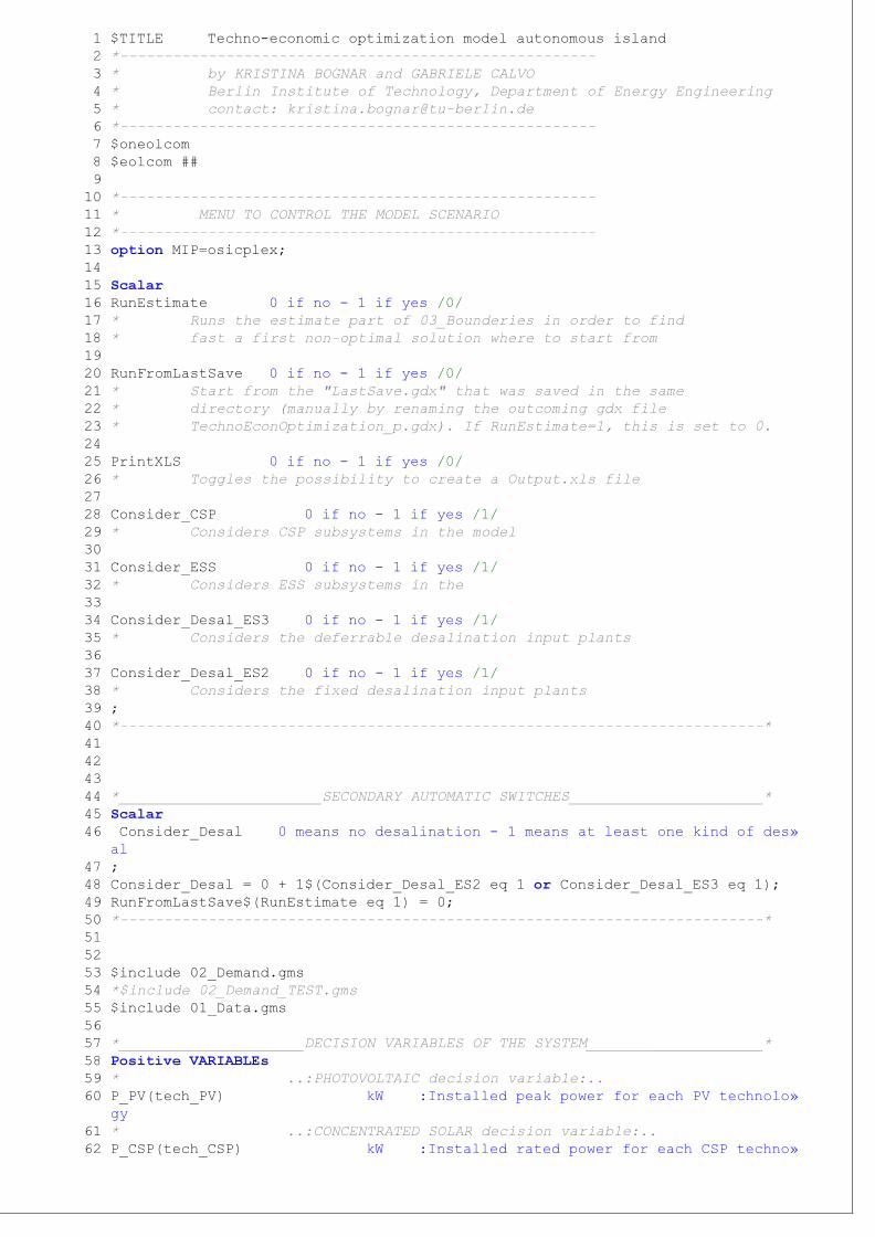
1 $TITLE Techno-economic optimization model autonomous island
2 *------------------------------------------------------
3 * by KRISTINA BOGNAR and GABRIELE CALVO
4 * Berlin Institute of Technology, Department of Energy Engineering
5 * contact: [email protected]
6 *------------------------------------------------------
7 $oneolcom
8 $eolcom ##
9
1 0 *------------------------------------------------------
1 1 * MENU TO CONTROL THE MODEL SCENARIO
1 2 *------------------------------------------------------
1 3 option MIP=osicplex;
1 4
1 5 Scalar
1 6 R u n E s t i m a t e 0 if no - 1 if yes /0/
1 7 * Runs the estimate part of 03_Bounderies in order to find
1 8 * fast a first non-optimal solution where to start from
1 9
2 0 R u n F r o m L a s t S a v e 0 if no - 1 if yes /0/
2 1 * Start from the "LastSave.gdx" that was saved in the same
2 2 * directory (manually by renaming the outcoming gdx file
2 3 * TechnoEconOptimization_p.gdx). If RunEstimate=1, this is set to 0.
2 4
2 5 P r i n t X L S 0 if no - 1 if yes /0/
2 6 * Toggles the possibility to create a Output.xls file
2 7
2 8 C o n s i d e r _ C S P 0 if no - 1 if yes /1/
2 9 * Considers CSP subsystems in the model
3 0
3 1 C o n s i d e r _ E S S 0 if no - 1 if yes /1/
3 2 * Considers ESS subsystems in the
3 3
3 4 C o n s i d e r _ D e s a l _ E S 3 0 if no - 1 if yes /1/
3 5 * Considers the deferrable desalination input plants
3 6
3 7 C o n s i d e r _ D e s a l _ E S 2 0 if no - 1 if yes /1/
3 8 * Considers the fixed desalination input plants
3 9 ;
4 0 *-------------------------------------------------------------------------*
4 1
4 2
4 3
4 4 *_______________________SECONDARY AUTOMATIC SWITCHES______________________*
4 5 Scalar
4 6 C o n s i d e r _ D e s a l 0 means no desalination - 1 means at least one kind of des»
al
4 7 ;
4 8 Consider_Desal = 0 + 1$(Consider_Desal_ES2 eq 1 or Consider_Desal_ES3 eq 1);
4 9 RunFromLastSave$(RunEstimate eq 1) = 0;
5 0 *-------------------------------------------------------------------------*
5 1
5 2
5 3 $include 02_Demand.gms
5 4 *$include 02_Demand_TEST.gms
5 5 $include 01_Data.gms
5 6
5 7 *_____________________DECISION VARIABLES OF THE SYSTEM____________________*
5 8 Positive VARIABLEs
5 9 * ..:PHOTOVOLTAIC decision variable:..
6 0 P_PV(tech_PV) kW :Installed peak power for each PV technolo»
gy
6 1 * ..:CONCENTRATED SOLAR decision variable:..
6 2 P_CSP(tech_CSP) kW :Installed rated power for each CSP techno»
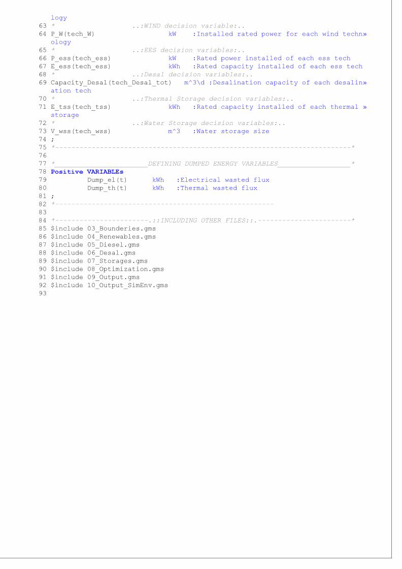
logy
6 3 * ..:WIND decision variable:..
6 4 P_W(tech_W) kW :Installed rated power for each wind techn»
ology
6 5 * ..:EES decision variables:..
6 6 P_ess(tech_ess) kW :Rated power installed of each ess tech
6 7 E_ess(tech_ess) kWh :Rated capacity installed of each ess tech
6 8 * ..:Desal decision variables:..
6 9 Capacity_Desal(tech_Desal_tot) m^3\d :Desalination capacity of each desalin»
ation tech
7 0 * ..:Thermal Storage decision variables:..
7 1 E_tss(tech_tss) kWh :Rated capacity installed of each thermal »
storage
7 2 * ..:Water Storage decision variables:..
7 3 V_wss(tech_wss) m^3 :Water storage size
7 4 ;
7 5 *-------------------------------------------------------------------------*
7 6
7 7 *_______________________DEFINING DUMPED ENERGY VARIABLES__________________*
7 8 Positive VARIABLEs
7 9 Dump_el(t) kWh :Electrical wasted flux
8 0 Dump_th(t) kWh :Thermal wasted flux
8 1 ;
8 2 *------------------------------------------------------
8 3
8 4 *-----------------------.::INCLUDING OTHER FILES::.-----------------------*
8 5 $include 03_Bounderies.gms
8 6 $include 04_Renewables.gms
8 7 $include 05_Diesel.gms
8 8 $include 06_Desal.gms
8 9 $include 07_Storages.gms
9 0 $include 08_Optimization.gms
9 1 $include 09_Output.gms
9 2 $include 10_Output_SimEnv.gms
9 3
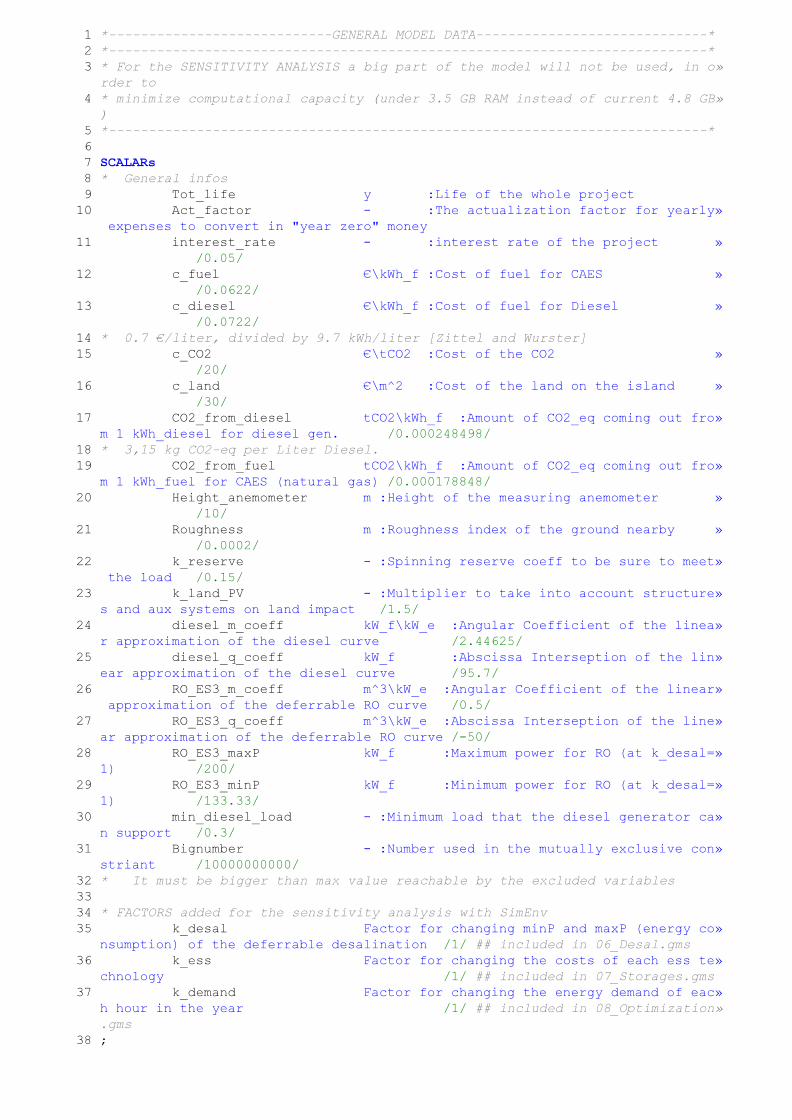
1 *----------------------------GENERAL MODEL DATA-----------------------------*
2 *---------------------------------------------------------------------------*
3 * For the SENSITIVITY ANALYSIS a big part of the model will not be used, in o»
rder to
4 * minimize computational capacity (under 3.5 GB RAM instead of current 4.8 GB»
)
5 *---------------------------------------------------------------------------*
6
7 SCALARs
8 * General infos
9 T o t _ l i f e y :Life of the whole project
1 0 A c t _ f a c t o r - :The actualization factor for yearly»
expenses to convert in "year zero" money
1 1 i n t e r e s t _ r a t e - :interest rate of the project »
/0.05/
1 2 c _ f u e l €\kWh_f :Cost of fuel for CAES »
/0.0622/
1 3 c _ d i e s e l €\kWh_f :Cost of fuel for Diesel »
/0.0722/
1 4 * 0.7 €/liter, divided by 9.7 kWh/liter [Zittel and Wurster]
1 5 c _ C O 2 €\tCO2 :Cost of the CO2 »
/20/
1 6 c _ l a n d €\m^2 :Cost of the land on the island »
/30/
1 7 C O 2 _ f r o m _ d i e s e l tCO2\kWh_f :Amount of CO2_eq coming out fro»
m 1 kWh_diesel for diesel gen. /0.000248498/
1 8 * 3,15 kg CO2-eq per Liter Diesel.
1 9 C O 2 _ f r o m _ f u e l tCO2\kWh_f :Amount of CO2_eq coming out fro»
m 1 kWh_fuel for CAES (natural gas) /0.000178848/
2 0 H e i g h t _ a n e m o m e t e r m :Height of the measuring anemometer »
/10/
2 1 R o u g h n e s s m :Roughness index of the ground nearby »
/0.0002/
2 2 k _ r e s e r v e - :Spinning reserve coeff to be sure to meet»
the load /0.15/
2 3 k _ l a n d _ P V - :Multiplier to take into account structure»
s and aux systems on land impact /1.5/
2 4 d i e s e l _ m _ c o e f f kW_f\kW_e :Angular Coefficient of the linea»
r approximation of the diesel curve /2.44625/
2 5 d i e s e l _ q _ c o e f f kW_f :Abscissa Interseption of the lin»
ear approximation of the diesel curve /95.7/
2 6 R O _ E S 3 _ m _ c o e f f m^3\kW_e :Angular Coefficient of the linear»
approximation of the deferrable RO curve /0.5/
2 7 R O _ E S 3 _ q _ c o e f f m^3\kW_e :Abscissa Interseption of the line»
ar approximation of the deferrable RO curve /-50/
2 8 R O _ E S 3 _ m a x P kW_f :Maximum power for RO (at k_desal=»
1 ) /200/
2 9 R O _ E S 3 _ m i n P kW_f :Minimum power for RO (at k_desal=»
1 ) /133.33/
3 0 m i n _ d i e s e l _ l o a d - :Minimum load that the diesel generator ca»
n support /0.3/
3 1 B i g n u m b e r - :Number used in the mutually exclusive con»
s t r i a n t /10000000000/
3 2 * It must be bigger than max value reachable by the excluded variables
3 3
3 4 * FACTORS added for the sensitivity analysis with SimEnv
3 5 k _ d e s a l Factor for changing minP and maxP (energy co»
nsumption) of the deferrable desalination /1/ ## included in 06_Desal.gms
3 6 k _ e s s Factor for changing the costs of each ess te»
c h n o l o g y /1/ ## included in 07_Storages.gms
3 7 k _ d e m a n d Factor for changing the energy demand of eac»
h hour in the year /1/ ## included in 08_Optimization»
.gms
3 8 ;
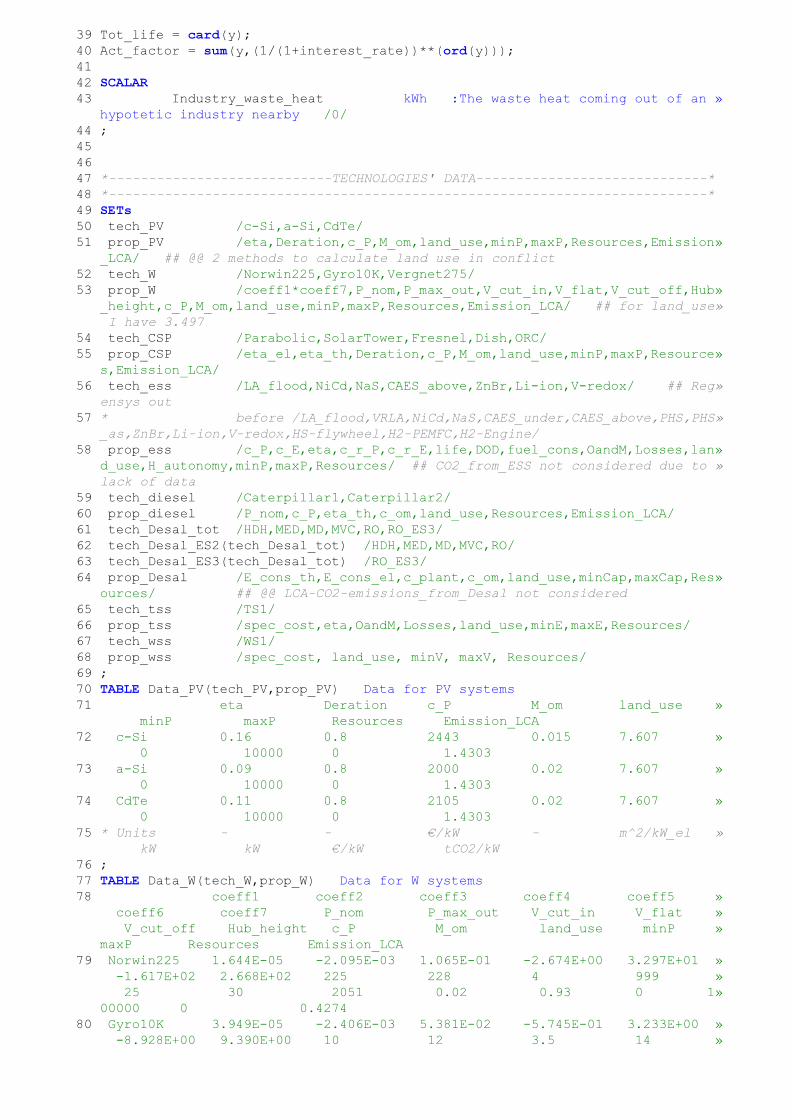
3 9 Tot_life = card(y);
4 0 Act_factor = sum(y,(1/(1+interest_rate))**(ord(y)));
4 1
4 2 SCALAR
4 3 I n d u s t r y _ w a s t e _ h e a t kWh :The waste heat coming out of an »
hypotetic industry nearby /0/
4 4 ;
4 5
4 6
4 7 *----------------------------TECHNOLOGIES' DATA-----------------------------*
4 8 *---------------------------------------------------------------------------*
4 9 SETs
5 0 t e c h _ P V /c-Si,a-Si,CdTe/
5 1 p r o p _ P V /eta,Deration,c_P,M_om,land_use,minP,maxP,Resources,Emission»
_LCA/ ## @@ 2 methods to calculate land use in conflict
5 2 t e c h _ W /Norwin225,Gyro10K,Vergnet275/
5 3 p r o p _ W /coeff1*coeff7,P_nom,P_max_out,V_cut_in,V_flat,V_cut_off,Hub»
_height,c_P,M_om,land_use,minP,maxP,Resources,Emission_LCA/ ## for land_use»
I have 3.497
5 4 t e c h _ C S P /Parabolic,SolarTower,Fresnel,Dish,ORC/
5 5 p r o p _ C S P /eta_el,eta_th,Deration,c_P,M_om,land_use,minP,maxP,Resource»
s,Emission_LCA/
5 6 t e c h _ e s s /LA_flood,NiCd,NaS,CAES_above,ZnBr,Li-ion,V-redox/ ## Reg»
ensys out
5 7 * before /LA_flood,VRLA,NiCd,NaS,CAES_under,CAES_above,PHS,PHS»
_as,ZnBr,Li-ion,V-redox,HS-flywheel,H2-PEMFC,H2-Engine/
5 8 p r o p _ e s s /c_P,c_E,eta,c_r_P,c_r_E,life,DOD,fuel_cons,OandM,Losses,lan»
d_use,H_autonomy,minP,maxP,Resources/ ## CO2_from_ESS not considered due to »
lack of data
5 9 t e c h _ d i e s e l /Caterpillar1,Caterpillar2/
6 0 p r o p _ d i e s e l /P_nom,c_P,eta_th,c_om,land_use,Resources,Emission_LCA/
6 1 t e c h _ D e s a l _ t o t /HDH,MED,MD,MVC,RO,RO_ES3/
6 2 tech_Desal_ES2(tech_Desal_tot) /HDH,MED,MD,MVC,RO/
6 3 tech_Desal_ES3(tech_Desal_tot) /RO_ES3/
6 4 p r o p _ D e s a l /E_cons_th,E_cons_el,c_plant,c_om,land_use,minCap,maxCap,Res»
ources/ ## @@ LCA-CO2-emissions_from_Desal not considered
6 5 t e c h _ t s s /TS1/
6 6 p r o p _ t s s /spec_cost,eta,OandM,Losses,land_use,minE,maxE,Resources/
6 7 t e c h _ w s s /WS1/
6 8 p r o p _ w s s /spec_cost, land_use, minV, maxV, Resources/
6 9 ;
7 0 TABLE Data_PV(tech_PV,prop_PV) Data for PV systems
7 1 eta Deration c_P M_om land_use »
minP maxP Resources Emission_LCA
7 2 c-Si 0.16 0.8 2443 0.015 7.607 »
0 10000 0 1.4303
7 3 a-Si 0.09 0.8 2000 0.02 7.607 »
0 10000 0 1.4303
7 4 CdTe 0.11 0.8 2105 0.02 7.607 »
0 10000 0 1.4303
7 5 * Units - - €/kW - m^2/kW_el »
kW kW €/kW tCO2/kW
7 6 ;
7 7 TABLE Data_W(tech_W,prop_W) Data for W systems
7 8 coeff1 coeff2 coeff3 coeff4 coeff5 »
coeff6 coeff7 P_nom P_max_out V_cut_in V_flat »
V_cut_off Hub_height c_P M_om land_use minP »
maxP Resources Emission_LCA
7 9 Norwin225 1.644E-05 -2.095E-03 1.065E-01 -2.674E+00 3.297E+01 »
-1.617E+02 2.668E+02 225 228 4 999 »
25 30 2051 0.02 0.93 0 1»
00000 0 0.4274
8 0 Gyro10K 3.949E-05 -2.406E-03 5.381E-02 -5.745E-01 3.233E+00 »
-8.928E+00 9.390E+00 10 12 3.5 14 »
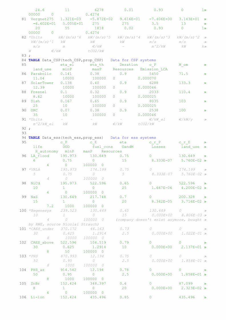
24.6 11 6278 0.01 0.93 0 1»
00000 0 0.4274
8 1 Vergnet275 1.321E-03 -5.872E-02 9.616E-01 -7.406E+00 3.143E+01 »
-6.602E+01 5.005E+01 275 275 3.5 13 »
20 55 1818 0.02 0.93 0 1»
00000 0 0.4274
8 2 *Units kW/(m/s)^6 kW/(m/s)^5 kW/(m/s)^4 kW/(m/s)^3 kW/(m/s)^2 »
kW/(m/s)^1 kW kW kW m/s m/s »
m/s m €/kW - m^2/kW kW k»
W €/kW tCO2/kW
8 3 ;
8 4 TABLE Data_CSP(tech_CSP,prop_CSP) Data for CSP systems
8 5 eta_el eta_th Deration c_P M_om »
land_use minP maxP Resources Emission_LCA
8 6 Parabolic 0.141 0.38 0.9 5450 71.5 »
11.04 10000 100000 0 0.000070
8 7 SolarTower 0.138 0.40 0.9 6288 133.3 »
12.39 10000 100000 0 0.000046
8 8 Fresnel 0.1 0.32 0.9 2033 110.4 »
8.62 10000 100000 0 0.000025
8 9 Dish 0.167 0.65 0.9 8035 103 »
25 10 100000 0 0.000025
9 0 ORC 0.07 0.38 0.9 2538 100 »
35 10 100000 0 0.000046
9 1 *Units - - - €/kW_el €/kW/y »
m^2/kW_el kW kW €/kW tCO2/kW
9 2 ;
9 3
9 4 TABLE Data_ess(tech_ess,prop_ess) Data for ess systems
9 5 c_P c_E eta c_r_P c_r_E »
life DOD fuel_cons OandM Losses land_use »
H_autonomy minP maxP Resources
9 6 LA_flood 195.973 130.649 0.75 0 130.649 »
6 0.75 0 15 8.333E-07 5.760E-02 »
4 0 100000 0
9 7 *VRLA 195.973 174.199 0.75 0 174.199 »
5 0.75 0 5 8.333E-07 5.760E-02 »
4 0 100000 0
9 8 NiCd 195.973 522.596 0.65 0 522.596 »
10 1 0 25 1.667E-06 4.200E-02 »
4 0 100000 0
9 9 NaS 130.649 217.748 0.7 0 200.328 »
15 1 0 20 8.342E-05 3.716E-02 »
7.2 1000 100000 0
1 0 0 *Regenesys 239.523 130.649 0.65 130.649 0 »
10 1 0 15 0.000E+00 8.806E-03 »
4 0 100000 0 (company doesn't exist anymore, bought »
by RWE, source Nicolai Strauch)
1 0 1 *CAES_under 370.172 46.163 0.73 0 0 »
30 0.625 1.2914 2.5 0.000E+00 1.022E-01 »
8 10000 100000 0
1 0 2 CAES_above 522.596 104.519 0.79 0 0 »
30 0.625 1.2914 10 0.000E+00 2.137E-01 »
8 50 100000 0
1 0 3 *PHS 870.993 12.194 0.75 0 0 »
50 0.95 0 2.5 0.000E+00 1.858E-01 »
8 1000 100000 0
1 0 4 PHS_as 914.542 12.194 0.78 0 0 »
50 0.95 0 2.5 0.000E+00 1.858E-01 »
8 1000 100000 0
1 0 5 ZnBr 152.424 348.397 0.6 0 87.099 »
8 1 0 20 0.000E+00 2.323E-02 »
4 0 100000 0
1 0 6 Li-ion 152.424 435.496 0.85 0 435.496 »
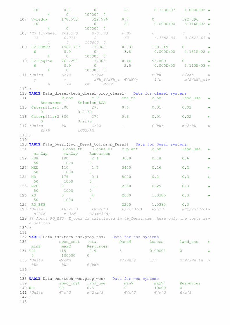
10 0.8 0 25 8.333E-07 1.000E-02 »
4 0 100000 0
1 0 7 V-redox 178.553 522.596 0.7 0 522.596 »
10 1 0 20 0.000E+00 3.716E-02 »
4 0 100000 0
1 0 8 *HS-flywheel 261.298 870.993 0.95 0 0 »
15 0.775 0 67 4.188E-04 3.252E-01 »
1 0 100000 0
1 0 9 H2-PEMFC 1567.787 13.065 0.531 130.649 0 »
6 0.9 0 3.8 0.000E+00 4.181E-02 »
4 0 100000 0
1 1 0 H2-Engine 261.298 13.065 0.44 95.809 0 »
6 0.9 0 2.5 0.000E+00 5.110E-03 »
4 0 100000 0
1 1 1 *Units €/kW €/kWh - €/kW €/kWh »
y - kWh_f/kWh_e €/kW/y 1/h m^2/kWh_el»
h kW kW €/kW
1 1 2 ;
1 1 3 TABLE Data_diesel(tech_diesel,prop_diesel) Data for diesel systems
1 1 4 P_nom c_P eta_th c_om land_use »
Resources Emission_LCA
1 1 5 Caterpillar1 800 270 0.6 0.01 0.02 »
0 0.2179
1 1 6 Caterpillar2 800 270 0.6 0.01 0.02 »
0 0.2179
1 1 7 *Units kW €/kW - €/kWh m^2/kW »
€/kW tCO2/kW
1 1 8 ;
1 1 9
1 2 0 TABLE Data_Desal(tech_Desal_tot,prop_Desal) Data for Desal systems
1 2 1 E_cons_th E_cons_el c_plant c_om land_use »
minCap maxCap Resources
1 2 2 HDH 100 2.4 3000 0.18 0.6 »
50 1000 0
1 2 3 MED 110 1.7 3400 0.16 0.2 »
50 1000 0
1 2 4 MD 175 0.1 5000 0.2 0.3 »
50 1000 0
1 2 5 MVC 0 11 2350 0.29 0.3 »
50 1000 0
1 2 6 RO 0 4 2000 1.0385 0.3 »
50 1000 0
1 2 7 RO_ES3 2200 1.0385 0.3
1 2 8 *Units kWh/m^3 kWh/m^3 €/(m^3/d) €/m^3 m^2/(m^3/d)»
m^3/d m^3/d €/(m^3/d)
1 2 9 ## About RO_ES3: E_cons is calculated in 06_Desal.gms, here only the costs ar»
e defined
1 3 0 ;
1 3 1
1 3 2 TABLE Data_tss(tech_tss,prop_tss) Data for tss systems
1 3 3 spec_cost eta OandM Losses land_use »
minE maxE Resources
1 3 4 TS1 115 0.9 5 0.00001 0 »
0 100000 0
1 3 5 *Units €/kWh - €/kWh/y 1/h m^2/kWh_th »
kWh kWh €/kWh
1 3 6 ;
1 3 7
1 3 8 TABLE Data_wss(tech_wss,prop_wss) Data for wss systems
1 3 9 spec_cost land_use minV maxV Resources
1 4 0 WS1 90 0.5 0 10000 0
1 4 1 *Units €\m^3 m^2\m^3 €/m^3 €/m^3 €/m^3
1 4 2 ;
1 4 3
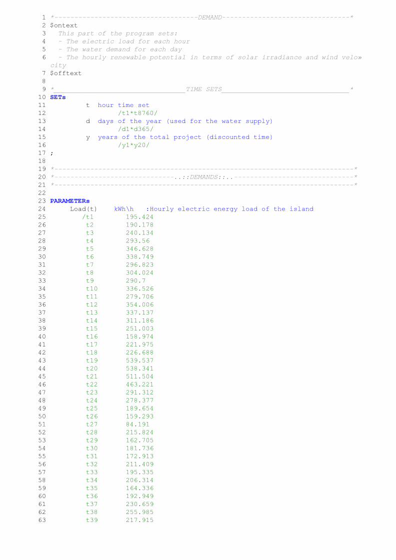
1 *------------------------------------DEMAND--------------------------------*
2 $ontext
3 This part of the program sets:
4 - The electric load for each hour
5 - The water demand for each day
6 - The hourly renewable potential in terms of solar irradiance and wind velo»
city
7 $offtext
8
9 *_________________________________TIME SETS________________________________*
1 0 SETs
1 1 t hour time set
1 2 /t1*t8760/
1 3 d days of the year (used for the water supply)
1 4 /d1*d365/
1 5 y years of the total project (discounted time)
1 6 /y1*y20/
1 7 ;
1 8
1 9 *---------------------------------------------------------------------------*
2 0 *------------------------------..::DEMANDS::..------------------------------*
2 1 *---------------------------------------------------------------------------*
2 2
2 3 PARAMETERs
2 4 Load(t) kWh\h :Hourly electric energy load of the island
2 5 /t1 195.424
2 6 t2 190.178
2 7 t3 240.134
2 8 t4 293.56
2 9 t5 346.628
3 0 t6 338.749
3 1 t7 296.823
3 2 t8 304.024
3 3 t9 290.7
3 4 t10 336.526
3 5 t11 279.706
3 6 t12 354.006
3 7 t13 337.137
3 8 t14 311.186
3 9 t15 251.003
4 0 t16 158.974
4 1 t17 221.975
4 2 t18 226.688
4 3 t19 539.537
4 4 t20 538.341
4 5 t21 511.504
4 6 t22 463.221
4 7 t23 291.312
4 8 t24 278.377
4 9 t25 189.654
5 0 t26 159.293
5 1 t27 84.191
5 2 t28 215.824
5 3 t29 162.705
5 4 t30 181.736
5 5 t31 172.913
5 6 t32 211.409
5 7 t33 195.335
5 8 t34 206.314
5 9 t35 164.336
6 0 t36 192.949
6 1 t37 230.659
6 2 t38 255.985
6 3 t39 217.915
6 4 t40 149.429
6 5 t41 166.735
6 6 t42 214.94
6 7 t43 285.186
6 8 t44 344.851
6 9 t45 342.128
7 0 t46 225.932
7 1 t47 189.405
7 2 t48 235.196
7 3 t49 233.127
7 4 t50 185.557
7 5 t51 188.626
7 6 t52 260.33
7 7 t53 278.788
7 8 t54 312.274
7 9 t55 276.516
8 0 t56 237.264
8 1 t57 277.27
8 2 t58 303.555
8 3 t59 273.142
8 4 t60 358.441
8 5 t61 268.698
8 6 t62 274.392
8 7 t63 224.468
8 8 t64 222.718
8 9 t65 214.44
9 0 t66 322.154
9 1 t67 527.342
9 2 t68 389.01
9 3 t69 453.253
9 4 t70 403.731
9 5 t71 380.326
9 6 t72 304.502
9 7 t73 182.454
9 8 t74 236.485
9 9 t75 220.288
1 0 0 t76 178.402
1 0 1 t77 194.537
1 0 2 t78 231.532
1 0 3 t79 279.736
1 0 4 t80 208.956
1 0 5 t81 213.735
1 0 6 t82 211.385
1 0 7 t83 330.49
1 0 8 t84 278.365
1 0 9 t85 234.232
1 1 0 t86 255.418
1 1 1 t87 232.148
1 1 2 t88 170.747
1 1 3 t89 135.448
1 1 4 t90 201.819
1 1 5 t91 506.667
1 1 6 t92 443.504
1 1 7 t93 352.518
1 1 8 t94 358.757
1 1 9 t95 296.324
1 2 0 t96 266.886
1 2 1 t97 145.055
1 2 2 t98 173.026
1 2 3 t99 157.388
1 2 4 t100 231.021
1 2 5 t101 184.121
1 2 6 t102 259.534
1 2 7 t103 202.608
8 7 6 8 t8744 259.624
8 7 6 9 t8745 252.764
8 7 7 0 t8746 294.054
8 7 7 1 t8747 309.254
8 7 7 2 t8748 176.248
8 7 7 3 t8749 291.225
8 7 7 4 t8750 281.174
8 7 7 5 t8751 244.528
8 7 7 6 t8752 310.246
8 7 7 7 t8753 236.526
8 7 7 8 t8754 280.518
8 7 7 9 t8755 516.816
8 7 8 0 t8756 507.19
8 7 8 1 t8757 483.84
8 7 8 2 t8758 349.617
8 7 8 3 t8759 374.79
8 7 8 4 t8760 238.389/
8 7 8 5
8 7 8 6 Water_demand(d) m^3\d :Daily water demand of the island
8 7 8 7 /set.d 800/
8 7 8 8 ;
8 7 8 9
8 7 9 0
8 7 9 1 *--------------------------------------------------------------------------*
8 7 9 2 *---------------------------..::POTENTIALS::..-----------------------------*
8 7 9 3 *--------------------------------------------------------------------------*
8 7 9 4
8 7 9 5 SET
8 7 9 6 m e t e o _ t y p e type of meteorologic data
8 7 9 7 /solar_radiation, wind_speed/
8 7 9 8 ;
8 7 9 9 TABLE
8 8 0 0 Potentials(t, meteo_type) solar and wind potentials
8 8 0 1 solar_radiation wind_speed
8 8 0 2 * [h] [kW/m2] [m/s]
8 8 0 3 t1 0 6.056
8 8 0 4 t2 0 5.2446
8 8 0 5 t3 0 4.7676
8 8 0 6 t4 0 1.603
8 8 0 7 t5 0 2.2279
8 8 0 8 t6 0 2.4148
8 8 0 9 t7 0 2.189
8 8 1 0 t8 0.03599 3.6099
8 8 1 1 t9 0.11261 3.5651
8 8 1 2 t10 0.23142 3.1687
8 8 1 3 t11 0.04872 4.9879
8 8 1 4 t12 0.0294 2.5256
8 8 1 5 t13 0.24638 2.1327
8 8 1 6 t14 0.22011 3.3471
8 8 1 7 t15 0.09044 2.5868
8 8 1 8 t16 0.05099 5.6994
8 8 1 9 t17 0.10904 6.7818
8 8 2 0 t18 0.05378 6.5577
8 8 2 1 t19 0.00555 4.1159
8 8 2 2 t20 0 6.5983
8 8 2 3 t21 0 8.0782
8 8 2 4 t22 0 6.8113
8 8 2 5 t23 0 4.2318
8 8 2 6 t24 0 4.9684
8 8 2 7 t25 0 5.6106
8 8 2 8 t26 0 5.3224
8 8 2 9 t27 0 6.492
8 8 3 0 t28 0 3.6051
8 8 3 1 t29 0 5.2886

1 *_______________________SOLVING THE MINIMUM OR 0 PROBLEM_____________________»
__*
2
3 Binary Variable ## To solve "0 or in range" problem
4 Exist_PV(tech_PV) 0 if csp not installed - 1 if installed
5 Exist_W(tech_W) 0 if csp not installed - 1 if installed
6 Exist_CSP(tech_CSP) 0 if csp not installed - 1 if installed
7 Exist_ess(tech_ess) 0 if ess not installed - 1 if installed
8 Exist_Desal(tech_Desal_ES2) 0 if Desal not installed - 1 if instal»
led
9 ;
1 0 Equations
1 1 minimumPV(tech_PV) sets the PV rated power to 0 or >= minP
1 2 maximumPV(tech_PV) sets the PV rated power to 0 or <= maxP
1 3 minimumW(tech_W) sets the CSP rated power to 0 or >= minP
1 4 maximumW(tech_W) sets the CSP rated power to 0 or <= maxP
1 5 minimumCSP(tech_CSP) sets the CSP rated power to 0 or >= minP
1 6 maximumCSP(tech_CSP) sets the CSP rated power to 0 or <= maxP
1 7 minimumEss_P(tech_ess) sets the Ess rated power to 0 or >= minP
1 8 maximumEss_P(tech_ess) sets the Ess rated power to 0 or <= maxP
1 9 minumumDesal(tech_Desal_ES2) sets the Desal capacity to 0 or >= minP
2 0 maximumDesal(tech_Desal_ES2) sets the Desal capacity to 0 or <= maxP
2 1 ;
2 2
2 3 minimumPV(tech_PV)..
2 4 P_PV(tech_PV) =g= Exist_PV(tech_PV)*Data_PV(tech_PV,'minP');
2 5 maximumPV(tech_PV)..
2 6 P_PV(tech_PV) =l= Exist_PV(tech_PV)*Data_PV(tech_PV,'maxP');
2 7 minimumW(tech_W)..
2 8 P_W(tech_W) =g= Exist_W(tech_W)*Data_W(tech_W,'minP');
2 9 maximumW(tech_W)..
3 0 P_W(tech_W) =l= Exist_W(tech_W)*Data_W(tech_W,'maxP');
3 1 minimumCSP(tech_CSP)$(Consider_CSP eq 1)..
3 2 P_CSP(tech_CSP) =g= Exist_CSP(tech_CSP)*Data_CSP(tech_CSP,'minP');
3 3 maximumCSP(tech_CSP)$(Consider_CSP eq 1)..
3 4 P_CSP(tech_CSP) =l= Exist_CSP(tech_CSP)*Data_CSP(tech_CSP,'maxP');
3 5 minimumEss_P(tech_ess)$(Consider_ESS eq 1)..
3 6 P_ess(tech_ess) =g= Exist_ess(tech_ess)*Data_ess(tech_ess,'minP');
3 7 maximumEss_P(tech_ess)$(Consider_ESS eq 1)..
3 8 P_ess(tech_ess) =l= Exist_ess(tech_ess)*Data_ess(tech_ess,'maxP');
3 9 minumumDesal(tech_Desal_ES2)$(Consider_Desal_ES2 eq 1)..
4 0 Capacity_Desal(tech_Desal_ES2) =g= Exist_Desal(tech_Desal_ES2)*Data_»
Desal(tech_Desal_ES2,'minCap');
4 1 maximumDesal(tech_Desal_ES2)$(Consider_Desal_ES2 eq 1)..
4 2 Capacity_Desal(tech_Desal_ES2) =l= Exist_Desal(tech_Desal_ES2)*Data_»
Desal(tech_Desal_ES2,'maxCap');
4 3
4 4 * Fixed water storage: 2 days autonomy
4 5 V_wss.fx('WS1')=2*Water_demand('d1'); ##To be changed if water demand not »
constant
4 6
4 7 $ontext
4 8 *No CSP
4 9 P_CSP.fx('Dish') = 0;
5 0 P_CSP.fx('ORC') = 0;
5 1
5 2 *Only RO (constant)
5 3 Capacity_Desal.fx('MVC') = 0;
5 4
5 5 *Only NaS
5 6 Exist_ess.fx('VRLA') = 0;
5 7 Exist_ess.fx('NiCd') = 0;
5 8 Exist_ess.fx('ZnBr') = 0;
5 9 Exist_ess.fx('Li-ion') = 0;
6 0 Exist_ess.fx('Li-ion') = 0;
6 1 $offtext
6 2
6 3
6 4
6 5 $ontext
6 6 *///////////////////////// RUN ESTIMATE VALUES //////////////////////
6 7 *__________ESTIMATE SCRIPT to find a first solution fast (not optimal)_______»
___
6 8 If (RunEstimate eq 1,
6 9 */////////////////////////////PHOTOVOLTAIC SYSTEM\\\\\\\\\\\\\\\\\\\\\\\\\\\\»
\\\
7 0 P_PV.fx('c-Si')=0;
7 1 P_PV.fx('a-Si')=0;
7 2 P_PV.fx('CdTe')=0;
7 3 */////////////////////////////////WIND SYSTEM\\\\\\\\\\\\\\\\\\\\\\\\\\\\\\\\»
\\\
7 4 P_W.fx('Norwin225')=0;
7 5 P_W.fx('Gyro10k')=0;
7 6 P_W.fx('Vergnet275')=1200;
7 7 *///////////////////////CONCENTRATED SOLAR POWER SYSTEM\\\\\\\\\\\\\\\\\\\\\\»
\\\
7 8 P_CSP.fx('Dish')=0;
7 9 P_CSP.fx('ORC')=0;
8 0 *///////////////////////////DESALINATION SYSTEM\\\\\\\\\\\\\\\\\\\\\\\\\\\\\\»
\\\
8 1 Exist_Desal.fx('HDH')=0; Capacity_Desal.fx('HDH')=0;
8 2 Exist_Desal.fx('MED')=0; Capacity_Desal.fx('MED')=0;
8 3 Exist_Desal.fx('MD')=0; Capacity_Desal.fx('MD')=0;
8 4 Exist_Desal.fx('MVC')=0; Capacity_Desal.fx('MVC')=0;
8 5 Exist_Desal.fx('RO')=1; Capacity_Desal.fx('RO')=800;
8 6 *////////////////////////ELECTRIC STORAGE SYSTEM\\\\\\\\\\\\\\\\\\\\\\\\\\\\\»
\\\
8 7 Exist_ess.fx('LA_flood')=0; P_ess.fx('LA_flood')=0;
8 8 Exist_ess.fx('CAES_above')=0; P_ess.fx('CAES_above')=0;
8 9 Exist_ess.fx('PHS')=1; P_ess.fx('PHS')=1000;
9 0 Exist_ess.fx('HS-flywheel')=0; P_ess.fx('HS-flywheel')=0;
9 1 Exist_ess.fx('Regenesys')=0; P_ess.fx('Regenesys')=0;
9 2 Exist_ess.fx('H2-Engine')=1; P_ess.fx('H2-Engine')=100;
9 3 *//////////////////////////THERMAL STORAGE SYSTEM\\\\\\\\\\\\\\\\\\\\\\\\\\\\»
\\\
9 4 E_tss.fx('TS1')=0;
9 5 *///////////////////////////WATER STORAGE SYSTEM\\\\\\\\\\\\\\\\\\\\\\\\\\\\\»
\\\
9 6 V_wss.l('WS1')=0;
9 7 );
9 8 $offtext
9 9
1 0 0
1 0 1 $ontext
1 0 2 *_______________________________________ESS SCREANING________________________»
__________________*
1 0 3 * If scenario = 1 all the ess' are set to 0, so no ess are taken into conside»
ration.
1 0 4 *P_ess.fx('LA_flood')$(Count_ESS eq 0) = Data_ess('LA_flood','minP'); »
Exist_ess.fx('LA_flood')$(Count_ESS eq 0)=0;
1 0 5 *P_ess.fx('Regenesys')$(Count_ESS eq 0) = Data_ess('Regenesys','minP'); »
Exist_ess.fx('Regenesys')$(Count_ESS eq 0)=0;
1 0 6 *P_ess.fx('PHS')$(Count_ESS eq 0) = Data_ess('PHS','minP'); »
Exist_ess.fx('PHS')$(Count_ESS eq 0)=0;
1 0 7 *P_ess.fx('CAES_above')$(Count_ESS eq 0) = Data_ess('CAES_above','minP'); »
Exist_ess.fx('CAES_above')$(Count_ESS eq 0)=0;
1 0 8 *P_ess.fx('HS-flywheel')$(Count_ESS eq 0) = Data_ess('HS-flywheel','minP'); »
Exist_ess.fx('HS-flywheel')$(Count_ESS eq 0)=0;
1 0 9 *P_ess.fx('H2-Engine')$(Count_ESS eq 0) = Data_ess('H2-Engine','minP'); »
Exist_ess.fx('H2-Engine')$(Count_ESS eq 0)=0;
1 1 0
1 1 1 ##Adjustments made to exclude PHS and include NaS (19/3/12)
1 1 2 *Exist_ess.fx('PHS')=0;
1 1 3 P_ess.fx('NaS')$(Count_ESS eq 0) = Data_ess('NaS','minP'); »
Exist_ess.fx('NaS')$(Count_ESS eq 0)=0;
1 1 4
1 1 5
1 1 6 *________.::ESS After prescreening::.
1 1 7 if (Prescreen_ESS eq 1 or Count_ESS eq 0,
1 1 8 P_ess.fx('VRLA') = 0; E_ess.fx('VRLA') = 0; Exist_ess.fx(»
'VRLA') =0;
1 1 9 P_ess.fx('NiCd') = 0; E_ess.fx('NiCd') = 0; Exist_ess.fx(»
'NiCd') =0;
1 2 0 *P_ess.fx('NaS') = 0; E_ess.fx('NaS') = 0; Exist_ess.fx»
('NaS') =0;
1 2 1 *P_ess.fx('CAES_under') = 0; E_ess.fx('CAES_under') = 0; Exist_ess.fx»
('CAES_under') =0;
1 2 2 *P_ess.fx('PHS_as') = 0; E_ess.fx('PHS_as') = 0; Exist_ess.fx»
('PHS_as') =0;
1 2 3 P_ess.fx('ZnBr') = 0; E_ess.fx('ZnBr') = 0; Exist_ess.fx(»
'ZnBr') =0;
1 2 4 P_ess.fx('Li-ion') = 0; E_ess.fx('Li-ion') = 0; Exist_ess.fx(»
'Li-ion') =0;
1 2 5 P_ess.fx('V-redox') = 0; E_ess.fx('V-redox') = 0; Exist_ess.fx(»
'V-redox') =0;
1 2 6 *P_ess.fx('H2-PEMFC') = 0; E_ess.fx('H2-PEMFC') = 0; Exist_ess.fx»
('H2-PEMFC') =0;
1 2 7 );
1 2 8
1 2 9 if (CountBigCSP eq 0,
1 3 0 *We already know that these techs are too big for PM
1 3 1 *P_CSP.fx('Parabolic') = 0;
1 3 2 *P_CSP.fx('SolarTower') = 0;
1 3 3 *P_CSP.fx('Fresnel') = 0;
1 3 4 )
1 3 5 */////////////////////////INITIAL_SETTINGS_end//////////////////////
1 3 6 $offtext
1 3 7
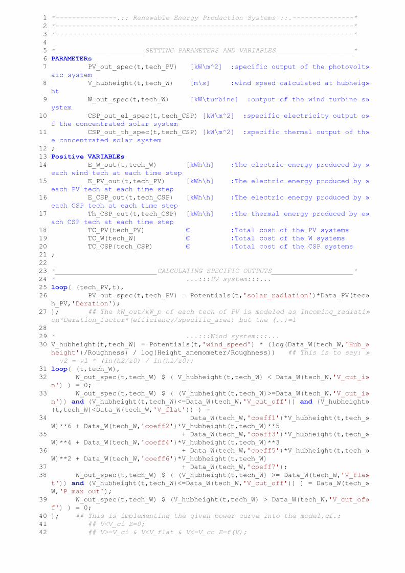
1 *---------------.:: Renewable Energy Production Systems ::.---------------*
2 *-------------------------------------------------------------------------*
3 *-------------------------------------------------------------------------*
4
5 *______________________SETTING PARAMETERS AND VARIABLES___________________*
6 PARAMETERs
7 PV_out_spec(t,tech_PV) [kW\m^2] :specific output of the photovolt»
aic system
8 V_hubheight(t,tech_W) [m\s] :wind speed calculated at hubheig»
ht
9 W_out_spec(t,tech_W) [kW\turbine] :output of the wind turbine s»
ystem
1 0 CSP_out_el_spec(t,tech_CSP) [kW\m^2] :specific electricity output o»
f the concentrated solar system
1 1 CSP_out_th_spec(t,tech_CSP) [kW\m^2] :specific thermal output of th»
e concentrated solar system
1 2 ;
1 3 Positive VARIABLEs
1 4 E_W_out(t,tech_W) [kWh\h] :The electric energy produced by »
each wind tech at each time step
1 5 E_PV_out(t,tech_PV) [kWh\h] :The electric energy produced by »
each PV tech at each time step
1 6 E_CSP_out(t,tech_CSP) [kWh\h] :The electric energy produced by »
each CSP tech at each time step
1 7 Th_CSP_out(t,tech_CSP) [kWh\h] :The thermal energy produced by e»
ach CSP tech at each time step
1 8 TC_PV(tech_PV) € :Total cost of the PV systems
1 9 TC_W(tech_W) € :Total cost of the W systems
2 0 TC_CSP(tech_CSP) € :Total cost of the CSP systems
2 1 ;
2 2
2 3 *_________________________CALCULATING SPECIFIC OUTPUTS____________________*
2 4 * ...:::PV system:::...
2 5 loop( (tech_PV,t),
2 6 PV_out_spec(t,tech_PV) = Potentials(t,'solar_radiation')*Data_PV(tec»
h_PV,'Deration');
2 7 ); ## The kW_out/kW_p of each tech of PV is modeled as Incoming_radiati»
on*Deration_factor*(efficiency/specific_area) but the (..)=1
2 8
2 9 * ...:::Wind system:::...
3 0 V_hubheight(t,tech_W) = Potentials(t,'wind_speed') * (log(Data_W(tech_W,'Hub_»
height')/Roughness) / log(Height_anemometer/Roughness)) ## This is to say: »
v2 = v1 * (ln(h2/z0) / ln(h1/z0))
3 1 loop( (t,tech_W),
3 2 W_out_spec(t,tech_W) $ ( V_hubheight(t,tech_W) < Data_W(tech_W,'V_cut_i»
n') ) = 0;
3 3 W_out_spec(t,tech_W) $ ( (V_hubheight(t,tech_W)>=Data_W(tech_W,'V_cut_i»
n')) and (V_hubheight(t,tech_W)<=Data_W(tech_W,'V_cut_off')) and (V_hubheight»
(t,tech_W)<Data_W(tech_W,'V_flat')) ) =
3 4 Data_W(tech_W,'coeff1')*V_hubheight(t,tech_»
W)**6 + Data_W(tech_W,'coeff2')*V_hubheight(t,tech_W)**5
3 5 + Data_W(tech_W,'coeff3')*V_hubheight(t,tech_»
W)**4 + Data_W(tech_W,'coeff4')*V_hubheight(t,tech_W)**3
3 6 + Data_W(tech_W,'coeff5')*V_hubheight(t,tech_»
W)**2 + Data_W(tech_W,'coeff6')*V_hubheight(t,tech_W)
3 7 + Data_W(tech_W,'coeff7');
3 8 W_out_spec(t,tech_W) $ ( (V_hubheight(t,tech_W) >= Data_W(tech_W,'V_fla»
t')) and (V_hubheight(t,tech_W)<=Data_W(tech_W,'V_cut_off')) ) = Data_W(tech_»
W,'P_max_out');
3 9 W_out_spec(t,tech_W) $ (V_hubheight(t,tech_W) > Data_W(tech_W,'V_cut_of»
f') ) = 0;
4 0 ); ## This is implementing the given power curve into the model,cf.:
4 1 ## V<V_ci E=0;
4 2 ## V>=V_ci & V<V_flat & V<=V_co E=f(V);
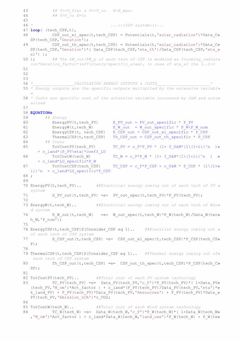
4 3 ## V>=V_flat & V<=V_co E=E_max;
4 4 ## V>V_co E=0;
4 5
4 6 * ...:::CSP system:::...
4 7 loop( (tech_CSP,t),
4 8 CSP_out_el_spec(t,tech_CSP) = Potentials(t,'solar_radiation')*Data_C»
SP(tech_CSP,'Deration');
4 9 CSP_out_th_spec(t,tech_CSP) = Potentials(t,'solar_radiation')*Data_C»
SP(tech_CSP,'Deration')*( Data_CSP(tech_CSP,'eta_th')/Data_CSP(tech_CSP,'eta_»
el') );
5 0 ); ## The kW_out/kW_p of each tech of CSP is modeled as Incoming_radiat»
ion*Deration_factor*(efficiency/specific_area), in case of eta_el the (..)=1
5 1
5 2
5 3
5 4 *_________________CALCULATING ENERGY OUTPUTS & COSTS______________________*
5 5 * Energy outputs are the specific outputs multiplied by the extensive variabl»
e
5 6 * Costs are specific cost of the extensive variable increased by O&M and actu»
alized
5 7
5 8 EQUATIONs
5 9 ## Energy
6 0 EnergyPV(t,tech_PV) E_PV_out = PV_out_specific * P_PV
6 1 EnergyW(t,tech_W) E_W_out = W_out_specific * P_W\P_W_nom
6 2 EnergyCSP(t, tech_CSP) E_CSP_out = CSP_out_el_specific * P_CSP
6 3 ThermalCSP(t,tech_CSP) Th_CSP_out = CSP_out_th_specific * P_CSP
6 4 ## Costs
6 5 TotCostPV(tech_PV) TC_PV = c_P*P_PV * (1+ f_O&M*(1\(1+i))^n )»
+ c_land*(P_PV\eta)*coeff_LU
6 6 TotCostW(tech_W) TC_W = c_P*P_W * (1+ f_O&M*(1\(1+i))^n ) »
+ c_land*LU_specific*P_W
6 7 TotCostCSP(tech_CSP) TC_CSP = c_P*P_CSP + c_O&M * P_CSP * (1\(1+»
i))^n + c_land*LU_specific*P_CSP
6 8 ;
6 9
7 0 EnergyPV(t,tech_PV).. ##Electrical energy coming out of each tech of PV »
system
7 1 E_PV_out(t,tech_PV) =e= PV_out_spec(t,tech_PV)*P_PV(tech_PV);
7 2
7 3 EnergyW(t,tech_W).. ##Electrical energy coming out of each tech of Win»
d system
7 4 E_W_out(t,tech_W) =e= W_out_spec(t,tech_W)*P_W(tech_W)/Data_W(tec»
h_W,'P_nom');
7 5
7 6 EnergyCSP(t,tech_CSP)$(Consider_CSP eq 1).. ##Electrial energy coming out »
of each tech of CSP system
7 7 E_CSP_out(t,tech_CSP) =e= CSP_out_el_spec(t,tech_CSP)*P_CSP(tech_CS»
P);
7 8
7 9 ThermalCSP(t,tech_CSP)$(Consider_CSP eq 1).. ##Thermal energy coming out of»
each tech of CSP system
8 0 Th_CSP_out(t,tech_CSP) =e= CSP_out_th_spec(t,tech_CSP)*P_CSP(tech_C»
SP);
8 1
8 2 TotCostPV(tech_PV).. ##Total cost of each PV system technology
8 3 TC_PV(tech_PV) =e= Data_PV(tech_PV,'c_P')*P_PV(tech_PV)*( 1+Data_PV»
(tech_PV,'M_om')*Act_factor ) + c_land*(P_PV(tech_PV)/Data_PV(tech_PV,'eta')*»
k_land_PV) + P_PV(tech_PV)*Data_PV(tech_PV,'Resources') + P_PV(tech_PV)*Data_»
PV(tech_PV,'Emission_LCA')*c_CO2;
8 4
8 5 TotCostW(tech_W).. ##Total cost of each Wind system technology
8 6 TC_W(tech_W) =e= Data_W(tech_W,'c_P')*P_W(tech_W)*( 1+Data_W(tech_W»
,'M_om')*Act_factor ) + c_land*Data_W(tech_W,'land_use')*P_W(tech_W) + P_W(te»

ch_W)*Data_W(tech_W,'Resources') + P_W(tech_W)*Data_W(tech_W,'Emission_LCA')*»
c_CO2;
8 7
8 8 TotCostCSP(tech_CSP)$(Consider_CSP eq 1).. ##Total cost of each CSP sys»
tem technology
8 9 TC_CSP(tech_CSP) =e= Data_CSP(tech_CSP,'c_P')*P_CSP(tech_CSP) + Dat»
a_CSP(tech_CSP,'M_om')*P_CSP(tech_CSP)*Act_factor + c_land*Data_CSP(tech_CSP»
,'land_use')*P_CSP(tech_CSP) + P_CSP(tech_CSP)*Data_CSP(tech_CSP,'Resources')»
+ P_CSP(tech_CSP)*Data_CSP(tech_CSP,'Emission_LCA')*c_CO2;
9 0
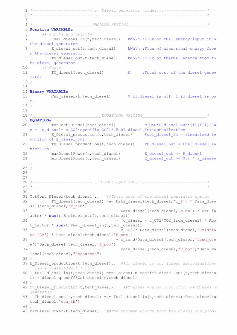
1 *-------------------------.:: Diesel generator model::.------------------*
2 *-------------------------------------------------------------------------*
3
4 *_________________________PROBLEM SETTING_________________________________*
5 Positive VARIABLEs
6 ## Inputs and outputs
7 Fuel_diesel_in(t,tech_diesel) kWh\h :Flux of fuel energy input in »
the diesel generator
8 E_diesel_out(t,tech_diesel) kWh\h :Flux of electrical energy fro»
m the diesel generator
9 Th_diesel_out(t,tech_diesel) kWh\h :Flux of thermal energy from t»
he diesel generator
1 0 ## Costs
1 1 TC_diesel(tech_diesel) € :Total cost of the diesel gene»
rator
1 2 ;
1 3
1 4 Binary VARIABLEs
1 5 Csi_diesel(t,tech_diesel) 0 if diesel is off. 1 if diesel is o»
n.
1 6 ;
1 7
1 8 *_____________________________EQUATIONS WRITING___________________________*
1 9 EQUATIONs
2 0 TotCost_Diesel(tech_diesel) c_O&M*E_diesel_out*(1\(1+i))^»
n + (c_diesel+ c_CO2*specific_CO2)*(Fuel_diesel_in)*actualization
2 1 E_Diesel_production(t,tech_diesel) Fuel_diesel_in = linearized f»
unction of E_diesel_out
2 2 Th_Diesel_production(t,tech_diesel) Th_diesel_out = Fuel_diesel_i»
n*eta_th
2 3 maxDieselPower(t,tech_diesel) E_diesel_out <= P_diesel
2 4 minDieselPower(t,tech_diesel) E_diesel_out >= 0.4 * P_diese»
l
2 5 ;
2 6
2 7
2 8 *-------------------------.::DIESEL EQUATIONS::.--------------------------*
2 9 *-------------------------------------------------------------------------*
3 0
3 1 TotCost_Diesel(tech_diesel).. ##Total cost of the diesel generator system
3 2 TC_diesel(tech_diesel) =e= Data_diesel(tech_diesel,'c_P') * Data_die»
sel(tech_diesel,'P_nom')
3 3 + Data_diesel(tech_diesel,'c_om') * Act_f»
actor * sum(t,E_diesel_out(t,tech_diesel))
3 4 + (c_diesel + c_CO2*CO2_from_diesel) * Ac»
t_factor * sum(t,Fuel_diesel_in(t,tech_diesel))
3 5 + c_CO2 * Data_diesel(tech_diesel,'Emissi»
on_LCA') * Data_diesel(tech_diesel,'P_nom')
3 6 + c_land*Data_diesel(tech_diesel,'land_us»
e')*Data_diesel(tech_diesel,'P_nom')
3 7 + Data_diesel(tech_diesel,"P_nom")*Data_d»
iesel(tech_diesel,"Resources")
3 8 ;
3 9 E_Diesel_production(t,tech_diesel).. ##If diesel is on, linear approximation»
: Fin = 2.44625*Eout + 95.7
4 0 Fuel_diesel_in(t,tech_diesel) =e= diesel_m_coeff*E_diesel_out(t,tech_diese»
l) + diesel_q_coeff*Csi_diesel(t,tech_diesel)
4 1 ;
4 2 Th_Diesel_production(t,tech_diesel).. ##Thermal energy production of diesel »
generator
4 3 Th_diesel_out(t,tech_diesel) =e= Fuel_diesel_in(t,tech_diesel)*Data_diesel(»
tech_diesel,'eta_th')
4 4 ;
4 5 maxDieselPower(t,tech_diesel).. ##The maximum energy that the diesel can prod»

uce in one hour
4 6 E_diesel_out(t,tech_diesel) =l= Csi_diesel(t,tech_diesel)* Data_diesel(tech»
_diesel,"P_nom")
4 7 ;
4 8 minDieselPower(t,tech_diesel).. ##The minimum energy load is 40%
4 9 E_diesel_out(t,tech_diesel) =g= Csi_diesel(t,tech_diesel)* min_diesel_load »
* Data_diesel(tech_diesel,"P_nom")
5 0 ;
5 1 * maxDieselPowerBasedOnConsumption(t,tech_diesel).. ##The maximum energy that»
the diesel can produce in one hour
5 2 * E_diesel_out(t,tech_diesel) =l= Csi_diesel(t,tech_diesel)* VERBRAUCH ZUM Z»
EITPUNKT T + maximale Entsalzung (Variable, die bereits definiert ist
5 3 ;
5 4
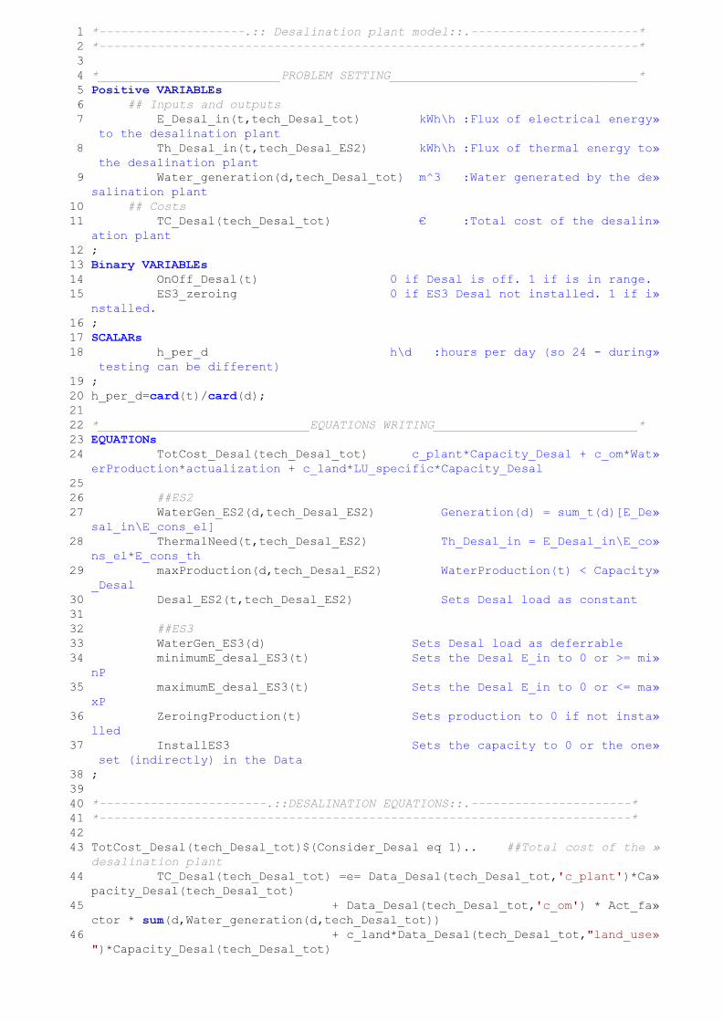
1 *--------------------.:: Desalination plant model::.-----------------------*
2 *--------------------------------------------------------------------------*
3
4 *_________________________PROBLEM SETTING__________________________________*
5 Positive VARIABLEs
6 ## Inputs and outputs
7 E_Desal_in(t,tech_Desal_tot) kWh\h :Flux of electrical energy»
to the desalination plant
8 Th_Desal_in(t,tech_Desal_ES2) kWh\h :Flux of thermal energy to»
the desalination plant
9 Water_generation(d,tech_Desal_tot) m^3 :Water generated by the de»
salination plant
1 0 ## Costs
1 1 TC_Desal(tech_Desal_tot) € :Total cost of the desalin»
ation plant
1 2 ;
1 3 Binary VARIABLEs
1 4 OnOff_Desal(t) 0 if Desal is off. 1 if is in range.
1 5 E S 3 _ z e r o i n g 0 if ES3 Desal not installed. 1 if i»
nstalled.
1 6 ;
1 7 SCALARs
1 8 h _ p e r _ d h\d :hours per day (so 24 - during»
testing can be different)
1 9 ;
2 0 h_per_d=card(t)/card(d);
2 1
2 2 *_____________________________EQUATIONS WRITING____________________________*
2 3 EQUATIONs
2 4 TotCost_Desal(tech_Desal_tot) c_plant*Capacity_Desal + c_om*Wat»
erProduction*actualization + c_land*LU_specific*Capacity_Desal
2 5
2 6 ##ES2
2 7 WaterGen_ES2(d,tech_Desal_ES2) Generation(d) = sum_t(d)[E_De»
sal_in\E_cons_el]
2 8 ThermalNeed(t,tech_Desal_ES2) Th_Desal_in = E_Desal_in\E_co»
ns_el*E_cons_th
2 9 maxProduction(d,tech_Desal_ES2) WaterProduction(t) < Capacity»
_Desal
3 0 Desal_ES2(t,tech_Desal_ES2) Sets Desal load as constant
3 1
3 2 ##ES3
3 3 WaterGen_ES3(d) Sets Desal load as deferrable
3 4 minimumE_desal_ES3(t) Sets the Desal E_in to 0 or >= mi»
nP
3 5 maximumE_desal_ES3(t) Sets the Desal E_in to 0 or <= ma»
xP
3 6 ZeroingProduction(t) Sets production to 0 if not insta»
lled
3 7 I n s t a l l E S 3 Sets the capacity to 0 or the one»
set (indirectly) in the Data
3 8 ;
3 9
4 0 *-----------------------.::DESALINATION EQUATIONS::.----------------------*
4 1 *-------------------------------------------------------------------------*
4 2
4 3 TotCost_Desal(tech_Desal_tot)$(Consider_Desal eq 1).. ##Total cost of the »
desalination plant
4 4 TC_Desal(tech_Desal_tot) =e= Data_Desal(tech_Desal_tot,'c_plant')*Ca»
pacity_Desal(tech_Desal_tot)
4 5 + Data_Desal(tech_Desal_tot,'c_om') * Act_fa»
ctor * sum(d,Water_generation(d,tech_Desal_tot))
4 6 + c_land*Data_Desal(tech_Desal_tot,"land_use»
")*Capacity_Desal(tech_Desal_tot)
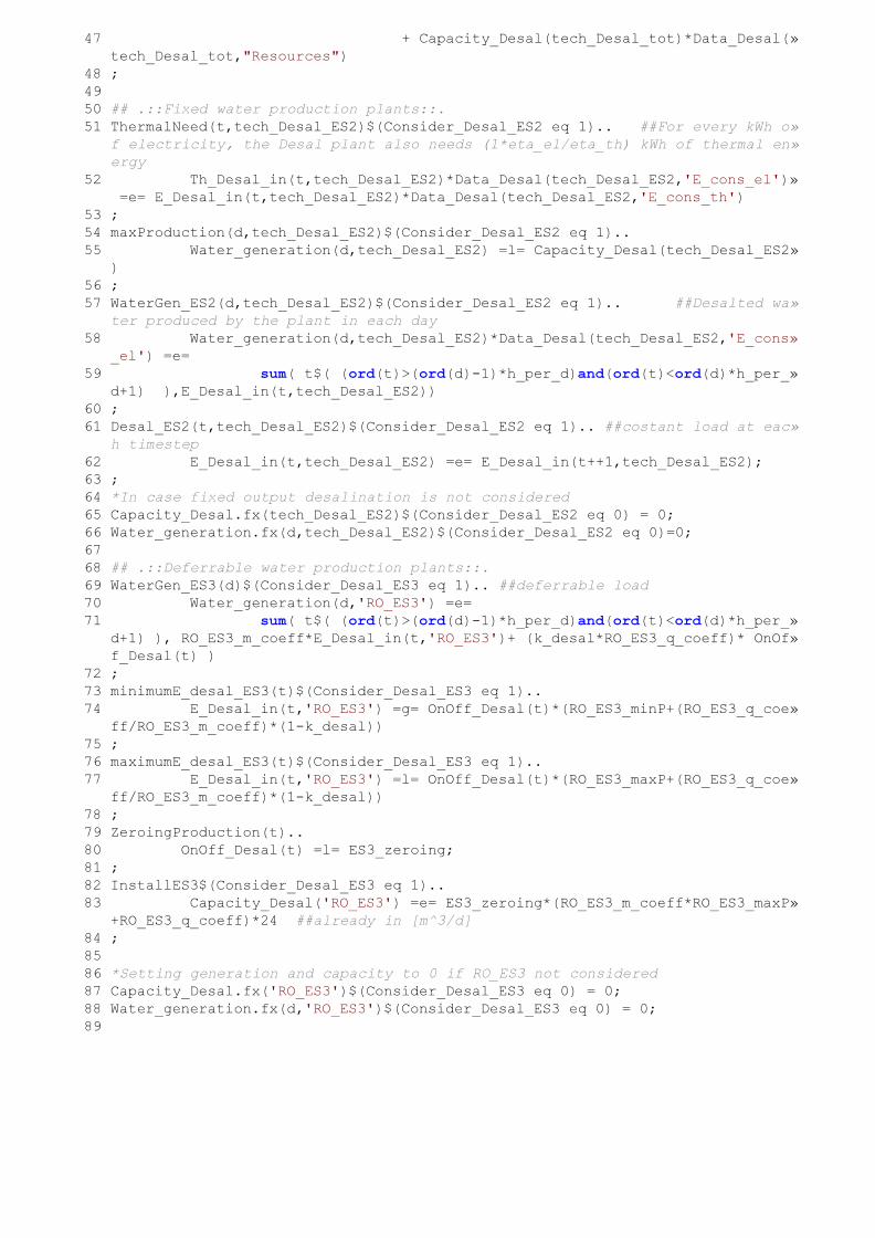
4 7 + Capacity_Desal(tech_Desal_tot)*Data_Desal(»
tech_Desal_tot,"Resources")
4 8 ;
4 9
5 0 ## .::Fixed water production plants::.
5 1 ThermalNeed(t,tech_Desal_ES2)$(Consider_Desal_ES2 eq 1).. ##For every kWh o»
f electricity, the Desal plant also needs (1*eta_el/eta_th) kWh of thermal en»
ergy
5 2 Th_Desal_in(t,tech_Desal_ES2)*Data_Desal(tech_Desal_ES2,'E_cons_el')»
=e= E_Desal_in(t,tech_Desal_ES2)*Data_Desal(tech_Desal_ES2,'E_cons_th')
5 3 ;
5 4 maxProduction(d,tech_Desal_ES2)$(Consider_Desal_ES2 eq 1)..
5 5 Water_generation(d,tech_Desal_ES2) =l= Capacity_Desal(tech_Desal_ES2»
)
5 6 ;
5 7 WaterGen_ES2(d,tech_Desal_ES2)$(Consider_Desal_ES2 eq 1).. ##Desalted wa»
ter produced by the plant in each day
5 8 Water_generation(d,tech_Desal_ES2)*Data_Desal(tech_Desal_ES2,'E_cons»
_el') =e=
5 9 sum( t$( (ord(t)>(ord(d)-1)*h_per_d)and(ord(t)<ord(d)*h_per_»
d+1) ),E_Desal_in(t,tech_Desal_ES2))
6 0 ;
6 1 Desal_ES2(t,tech_Desal_ES2)$(Consider_Desal_ES2 eq 1).. ##costant load at eac»
h timestep
6 2 E_Desal_in(t,tech_Desal_ES2) =e= E_Desal_in(t++1,tech_Desal_ES2);
6 3 ;
6 4 *In case fixed output desalination is not considered
6 5 Capacity_Desal.fx(tech_Desal_ES2)$(Consider_Desal_ES2 eq 0) = 0;
6 6 Water_generation.fx(d,tech_Desal_ES2)$(Consider_Desal_ES2 eq 0)=0;
6 7
6 8 ## .::Deferrable water production plants::.
6 9 WaterGen_ES3(d)$(Consider_Desal_ES3 eq 1).. ##deferrable load
7 0 Water_generation(d,'RO_ES3') =e=
7 1 sum( t$( (ord(t)>(ord(d)-1)*h_per_d)and(ord(t)<ord(d)*h_per_»
d+1) ), RO_ES3_m_coeff*E_Desal_in(t,'RO_ES3')+ (k_desal*RO_ES3_q_coeff)* OnOf»
f_Desal(t) )
7 2 ;
7 3 minimumE_desal_ES3(t)$(Consider_Desal_ES3 eq 1)..
7 4 E_Desal_in(t,'RO_ES3') =g= OnOff_Desal(t)*(RO_ES3_minP+(RO_ES3_q_coe»
ff/RO_ES3_m_coeff)*(1-k_desal))
7 5 ;
7 6 maximumE_desal_ES3(t)$(Consider_Desal_ES3 eq 1)..
7 7 E_Desal_in(t,'RO_ES3') =l= OnOff_Desal(t)*(RO_ES3_maxP+(RO_ES3_q_coe»
ff/RO_ES3_m_coeff)*(1-k_desal))
7 8 ;
7 9 ZeroingProduction(t)..
8 0 OnOff_Desal(t) =l= ES3_zeroing;
8 1 ;
8 2 InstallES3$(Consider_Desal_ES3 eq 1)..
8 3 Capacity_Desal('RO_ES3') =e= ES3_zeroing*(RO_ES3_m_coeff*RO_ES3_maxP»
+RO_ES3_q_coeff)*24 ##already in [m^3/d]
8 4 ;
8 5
8 6 *Setting generation and capacity to 0 if RO_ES3 not considered
8 7 Capacity_Desal.fx('RO_ES3')$(Consider_Desal_ES3 eq 0) = 0;
8 8 Water_generation.fx(d,'RO_ES3')$(Consider_Desal_ES3 eq 0) = 0;
8 9
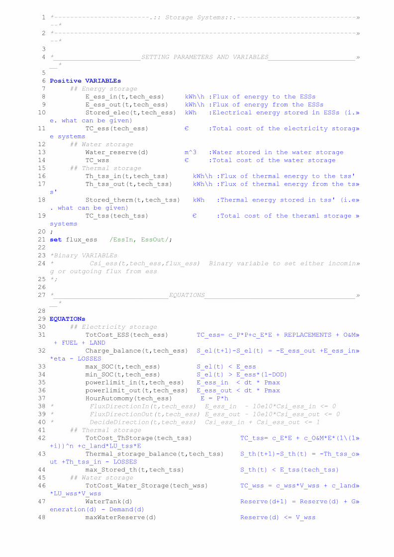
1 *------------------------.:: Storage Systems::.------------------------------»
--*
2 *----------------------------------------------------------------------------»
--*
3
4 *______________________SETTING PARAMETERS AND VARIABLES______________________»
__*
5
6 Positive VARIABLEs
7 ## Energy storage
8 E_ess_in(t,tech_ess) kWh\h :Flux of energy to the ESSs
9 E_ess_out(t,tech_ess) kWh\h :Flux of energy from the ESSs
1 0 Stored_elec(t,tech_ess) kWh :Electrical energy stored in ESSs (i.»
e. what can be given)
1 1 TC_ess(tech_ess) € :Total cost of the electricity storag»
e systems
1 2 ## Water storage
1 3 Water_reserve(d) m^3 :Water stored in the water storage
1 4 T C _ w s s € :Total cost of the water storage
1 5 ## Thermal storage
1 6 Th_tss_in(t,tech_tss) kWh\h :Flux of thermal energy to the tss'
1 7 Th_tss_out(t,tech_tss) kWh\h :Flux of thermal energy from the ts»
s'
1 8 Stored_therm(t,tech_tss) kWh :Thermal energy stored in tss' (i.e»
. what can be given)
1 9 TC_tss(tech_tss) € :Total cost of the theraml storage »
systems
2 0 ;
2 1 set f l u x _ e s s /EssIn, EssOut/;
2 2
2 3 *Binary VARIABLEs
2 4 * Csi_ess(t,tech_ess,flux_ess) Binary variable to set either incomin»
g or outgoing flux from ess
2 5 *;
2 6
2 7 *_____________________________EQUATIONS______________________________________»
__*
2 8
2 9 EQUATIONs
3 0 ## Electricity storage
3 1 TotCost_ESS(tech_ess) TC_ess= c_P*P+c_E*E + REPLACEMENTS + O&M»
+ FUEL + LAND
3 2 Charge_balance(t,tech_ess) S_el(t+1)-S_el(t) = -E_ess_out +E_ess_in»
*eta - LOSSES
3 3 max_SOC(t,tech_ess) S_el(t) < E_ess
3 4 min_SOC(t,tech_ess) S_el(t) > E_ess*(1-DOD)
3 5 powerlimit_in(t,tech_ess) E_ess_in < dt * Pmax
3 6 powerlimit_out(t,tech_ess) E_ess_out < dt * Pmax
3 7 HourAutomomy(tech_ess) E = P*h
3 8 * FluxDirectionIn(t,tech_ess) E_ess_in - 10e10*Csi_ess_in <= 0
3 9 * FluxDirectionOut(t,tech_ess) E_ess_out - 10e10*Csi_ess_out <= 0
4 0 * DecideDirection(t,tech_ess) Csi_ess_in + Csi_ess_out <= 1
4 1 ## Thermal storage
4 2 TotCost_ThStorage(tech_tss) TC_tss= c_E*E + c_O&M*E*(1\(1»
+i))^n +c_land*LU_tss*E
4 3 Thermal_storage_balance(t,tech_tss) S_th(t+1)-S_th(t) = -Th_tss_o»
ut +Th_tss_in - LOSSES
4 4 max_Stored_th(t,tech_tss) S_th(t) < E_tss(tech_tss)
4 5 ## Water storage
4 6 TotCost_Water_Storage(tech_wss) TC_wss = c_wss*V_wss + c_land»
*LU_wss*V_wss
4 7 WaterTank(d) Reserve(d+1) = Reserve(d) + G»
eneration(d) - Demand(d)
4 8 maxWaterReserve(d) Reserve(d) <= V_wss
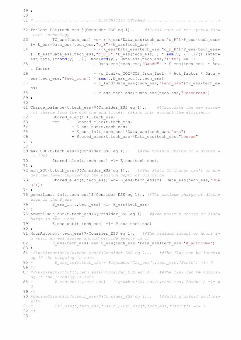
4 9 ;
5 0
5 1 *...........................ELECTRICITY STORAGE..............................»
...
5 2 TotCost_ESS(tech_ess)$(Consider_ESS eq 1).. ##Total cost of the system for»
each technology
5 3 TC_ess(tech_ess) =e= ( k_ess*Data_ess(tech_ess,"c_P")*P_ess(tech_ess»
)+ k_ess*Data_ess(tech_ess,"c_E")*E_ess(tech_ess) )
5 4 + ( k_ess*Data_ess(tech_ess,"c_r_P")*P_ess(tech_ess»
)+ k_ess*Data_ess(tech_ess,"c_r_E")*E_ess(tech_ess) ) * sum(y, ( (1/(1+inter»
est_rate))**ord(y) )$( mod(ord(y), Data_ess(tech_ess,"life"))=0 ) )
5 5 + Data_ess(tech_ess,"OandM") * P_ess(tech_ess) * Ac»
t_factor
5 6 + (c_fuel+c_CO2*CO2_from_fuel) * Act_factor * Data_»
ess(tech_ess,"fuel_cons") * sum(t,E_ess_out(t,tech_ess))
5 7 + c_land*Data_ess(tech_ess,"land_use")*E_ess(tech_e»
ss)
5 8 + P_ess(tech_ess)*Data_ess(tech_ess,"Resources")
5 9 ;
6 0
6 1 Charge_balance(t,tech_ess)$(Consider_ESS eq 1).. ##Calculate the new state»
of charge from the old one and fluxes, taking into account the efficiency
6 2 Stored_elec(t++1,tech_ess)
6 3 =e= + Stored_elec(t,tech_ess)
6 4 - E_ess_out(t,tech_ess)
6 5 + E_ess_in(t,tech_ess)*Data_ess(tech_ess,"eta")
6 6 - Stored_elec(t,tech_ess)*Data_ess(tech_ess,"Losses")
6 7 ;
6 8
6 9 max_SOC(t,tech_ess)$(Consider_ESS eq 1).. ##The maximum charge of a system »
is 100%
7 0 Stored_elec(t,tech_ess) =l= E_ess(tech_ess);
7 1 ;
7 2 min_SOC(t,tech_ess)$(Consider_ESS eq 1).. ##The State Of Charge can't go un»
der the level imposed by the maximum Depth of Discharge
7 3 Stored_elec(t,tech_ess) =g= E_ess(tech_ess)*(1-Data_ess(tech_ess,'DO»
D'));
7 4 ;
7 5 powerlimit_in(t,tech_ess)$(Consider_ESS eq 1).. ##The maximum charge or disch»
arge is the P_ess
7 6 E_ess_in(t,tech_ess) =l= P_ess(tech_ess)
7 7 ;
7 8 powerlimit_out(t,tech_ess)$(Consider_ESS eq 1).. ##The maximum charge or disc»
harge is the P_ess
7 9 E_ess_out(t,tech_ess) =l= P_ess(tech_ess)
8 0 ;
8 1 HourAutomomy(tech_ess)$(Consider_ESS eq 1).. ##The minimum amount of hours i»
n which an ess system should provide energy is 1h
8 2 E_ess(tech_ess) =e= P_ess(tech_ess)*Data_ess(tech_ess,'H_autonomy')
8 3 ;
8 4 *FluxDirectionIn(t,tech_ess)$(Consider_ESS eq 1).. ##The flux can be incomi»
ng if the outgoing is zero
8 5 * E_ess_in(t,tech_ess)- Bignumber*Csi_ess(t,tech_ess,'EssIn') =l= 0
8 6 *;
8 7 *FluxDirectionOut(t,tech_ess)$(Consider_ESS eq 1).. ##The flux can be outgoi»
ng if the incoming is zero
8 8 * E_ess_out(t,tech_ess) - Bignumber*Csi_ess(t,tech_ess,'EssOut') =l= »
0
8 9 *;
9 0 *DecideDirection(t,tech_ess)$(Consider_ESS eq 1).. ##Setting mutual exclusi»
vity
9 1 * Csi_ess(t,tech_ess,'EssIn')+Csi_ess(t,tech_ess,'EssOut') =l= 1
9 2 *;
9 3
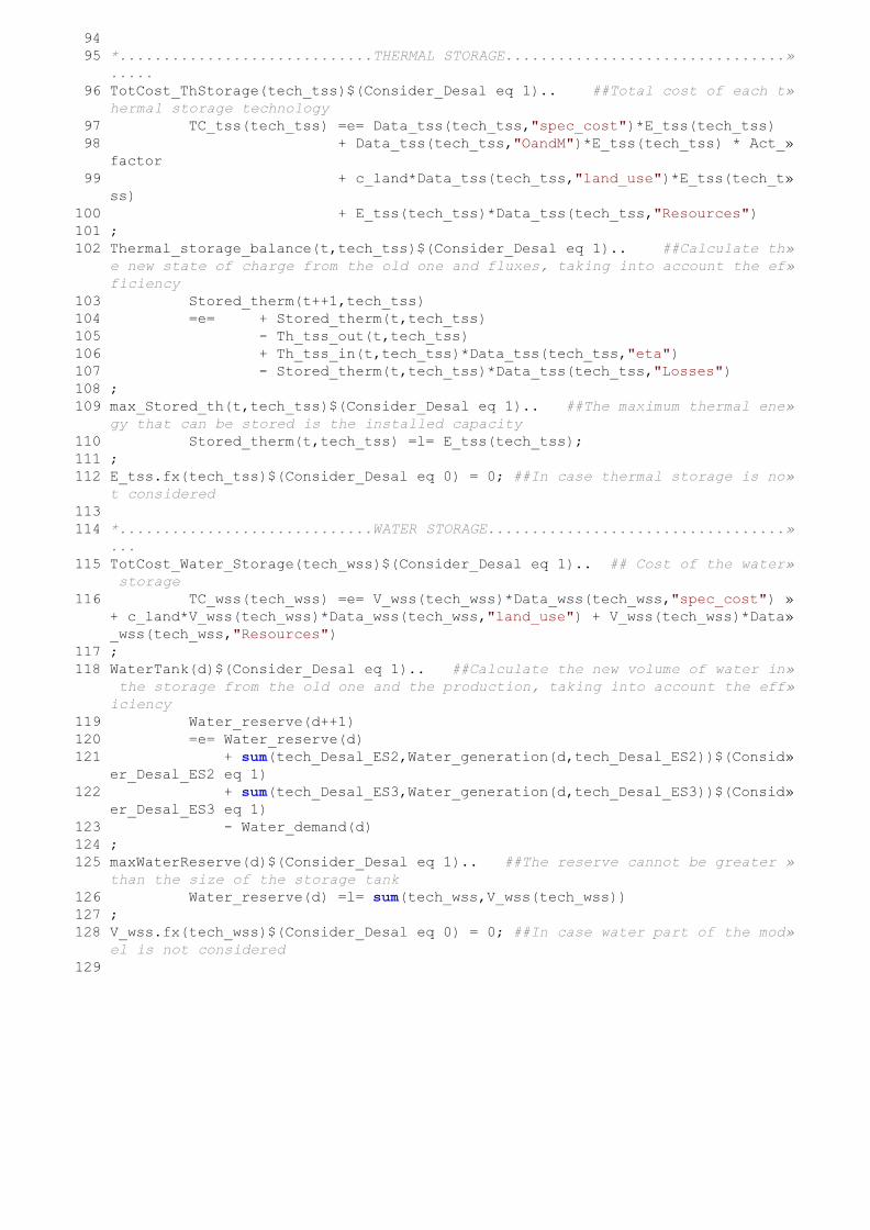
9 4
9 5 *.............................THERMAL STORAGE................................»
.....
9 6 TotCost_ThStorage(tech_tss)$(Consider_Desal eq 1).. ##Total cost of each t»
hermal storage technology
9 7 TC_tss(tech_tss) =e= Data_tss(tech_tss,"spec_cost")*E_tss(tech_tss)
9 8 + Data_tss(tech_tss,"OandM")*E_tss(tech_tss) * Act_»
factor
9 9 + c_land*Data_tss(tech_tss,"land_use")*E_tss(tech_t»
ss)
1 0 0 + E_tss(tech_tss)*Data_tss(tech_tss,"Resources")
1 0 1 ;
1 0 2 Thermal_storage_balance(t,tech_tss)$(Consider_Desal eq 1).. ##Calculate th»
e new state of charge from the old one and fluxes, taking into account the ef»
ficiency
1 0 3 Stored_therm(t++1,tech_tss)
1 0 4 =e= + Stored_therm(t,tech_tss)
1 0 5 - Th_tss_out(t,tech_tss)
1 0 6 + Th_tss_in(t,tech_tss)*Data_tss(tech_tss,"eta")
1 0 7 - Stored_therm(t,tech_tss)*Data_tss(tech_tss,"Losses")
1 0 8 ;
1 0 9 max_Stored_th(t,tech_tss)$(Consider_Desal eq 1).. ##The maximum thermal ene»
gy that can be stored is the installed capacity
1 1 0 Stored_therm(t,tech_tss) =l= E_tss(tech_tss);
1 1 1 ;
1 1 2 E_tss.fx(tech_tss)$(Consider_Desal eq 0) = 0; ##In case thermal storage is no»
t considered
1 1 3
1 1 4 *.............................WATER STORAGE..................................»
...
1 1 5 TotCost_Water_Storage(tech_wss)$(Consider_Desal eq 1).. ## Cost of the water»
s t o r a g e
1 1 6 TC_wss(tech_wss) =e= V_wss(tech_wss)*Data_wss(tech_wss,"spec_cost") »
+ c_land*V_wss(tech_wss)*Data_wss(tech_wss,"land_use") + V_wss(tech_wss)*Data»
_wss(tech_wss,"Resources")
1 1 7 ;
1 1 8 WaterTank(d)$(Consider_Desal eq 1).. ##Calculate the new volume of water in»
the storage from the old one and the production, taking into account the eff»
iciency
1 1 9 Water_reserve(d++1)
1 2 0 =e= Water_reserve(d)
1 2 1 + sum(tech_Desal_ES2,Water_generation(d,tech_Desal_ES2))$(Consid»
er_Desal_ES2 eq 1)
1 2 2 + sum(tech_Desal_ES3,Water_generation(d,tech_Desal_ES3))$(Consid»
er_Desal_ES3 eq 1)
1 2 3 - Water_demand(d)
1 2 4 ;
1 2 5 maxWaterReserve(d)$(Consider_Desal eq 1).. ##The reserve cannot be greater »
than the size of the storage tank
1 2 6 Water_reserve(d) =l= sum(tech_wss,V_wss(tech_wss))
1 2 7 ;
1 2 8 V_wss.fx(tech_wss)$(Consider_Desal eq 0) = 0; ##In case water part of the mod»
el is not considered
1 2 9
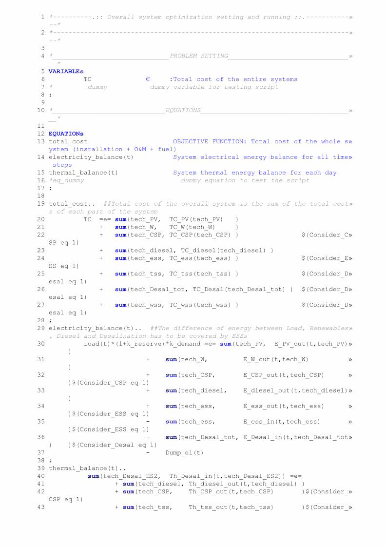
1 *----------.:: Overall system optimization setting and running ::.-----------»
--*
2 *----------------------------------------------------------------------------»
--*
3
4 *______________________________PROBLEM SETTING_______________________________»
__*
5 VARIABLEs
6 T C € :Total cost of the entire systems
7 * dummy dummy variable for testing script
8 ;
9
1 0 *_____________________________EQUATIONS______________________________________»
__*
1 1
1 2 EQUATIONs
1 3 t o t a l _ c o s t OBJECTIVE FUNCTION: Total cost of the whole s»
ystem (installation + O&M + fuel)
1 4 electricity_balance(t) System electrical energy balance for all time»
s t e p s
1 5 thermal_balance(t) System thermal energy balance for each day
1 6 *eq_dummy dummy equation to test the script
1 7 ;
1 8
1 9 total_cost.. ##Total cost of the overall system is the sum of the total cost»
s of each part of the system
2 0 TC =e= sum(tech_PV, TC_PV(tech_PV) )
2 1 + sum(tech_W, TC_W(tech_W) )
2 2 + sum(tech_CSP, TC_CSP(tech_CSP) ) $(Consider_C»
SP eq 1)
2 3 + sum(tech_diesel, TC_diesel(tech_diesel) )
2 4 + sum(tech_ess, TC_ess(tech_ess) ) $(Consider_E»
SS eq 1)
2 5 + sum(tech_tss, TC_tss(tech_tss) ) $(Consider_D»
esal eq 1)
2 6 + sum(tech_Desal_tot, TC_Desal(tech_Desal_tot) ) $(Consider_D»
esal eq 1)
2 7 + sum(tech_wss, TC_wss(tech_wss) ) $(Consider_D»
esal eq 1)
2 8 ;
2 9 electricity_balance(t).. ##The difference of energy between Load, Renewables»
, Diesel and Desalination has to be covered by ESSs
3 0 Load(t)*(1+k_reserve)*k_demand =e= sum(tech_PV, E_PV_out(t,tech_PV)»
)
3 1 + sum(tech_W, E_W_out(t,tech_W) »
)
3 2 + sum(tech_CSP, E_CSP_out(t,tech_CSP) »
)$(Consider_CSP eq 1)
3 3 + sum(tech_diesel, E_diesel_out(t,tech_diesel)»
)
3 4 + sum(tech_ess, E_ess_out(t,tech_ess) »
)$(Consider_ESS eq 1)
3 5 - sum(tech_ess, E_ess_in(t,tech_ess) »
)$(Consider_ESS eq 1)
3 6 - sum(tech_Desal_tot, E_Desal_in(t,tech_Desal_tot»
) )$(Consider_Desal eq 1)
3 7 - Dump_el(t)
3 8 ;
3 9 thermal_balance(t)..
4 0 sum(tech_Desal_ES2, Th_Desal_in(t,tech_Desal_ES2)) =e=
4 1 + sum(tech_diesel, Th_diesel_out(t,tech_diesel) )
4 2 + sum(tech_CSP, Th_CSP_out(t,tech_CSP) )$(Consider_»
CSP eq 1)
4 3 + sum(tech_tss, Th_tss_out(t,tech_tss) )$(Consider_»
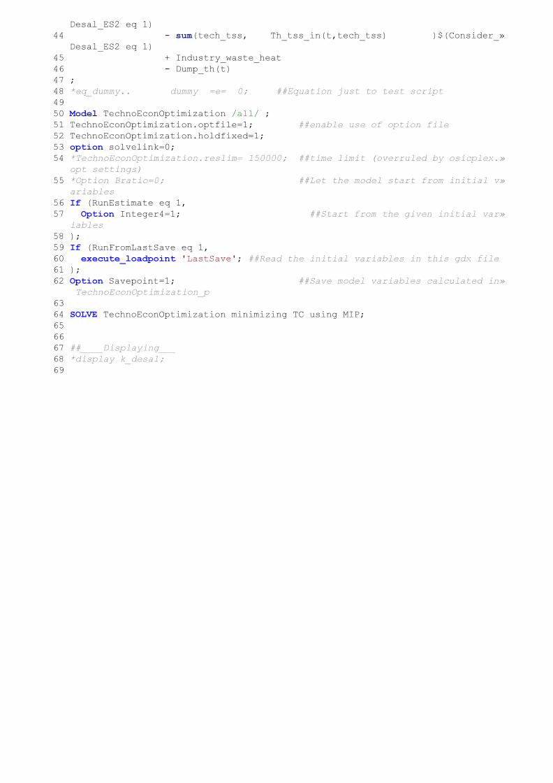
Desal_ES2 eq 1)
4 4 - sum(tech_tss, Th_tss_in(t,tech_tss) )$(Consider_»
Desal_ES2 eq 1)
4 5 + Industry_waste_heat
4 6 - Dump_th(t)
4 7 ;
4 8 *eq_dummy.. dummy =e= 0; ##Equation just to test script
4 9
5 0 Model TechnoEconOptimization /all/ ;
5 1 TechnoEconOptimization.optfile=1; ##enable use of option file
5 2 TechnoEconOptimization.holdfixed=1;
5 3 option solvelink=0;
5 4 *TechnoEconOptimization.reslim= 150000; ##time limit (overruled by osicplex.»
opt settings)
5 5 *Option Bratio=0; ##Let the model start from initial v»
ariables
5 6 If (RunEstimate eq 1,
5 7 Option Integer4=1; ##Start from the given initial var»
iables
5 8 );
5 9 If (RunFromLastSave eq 1,
6 0 execute_loadpoint 'LastSave'; ##Read the initial variables in this gdx file
6 1 );
6 2 Option Savepoint=1; ##Save model variables calculated in»
T e c h n o E c o n O p t i m i z a t i o n _ p
6 3
6 4 SOLVE TechnoEconOptimization minimizing TC using MIP;
6 5
6 6
6 7 ##____Displaying___
6 8 *display k_desal;
6 9
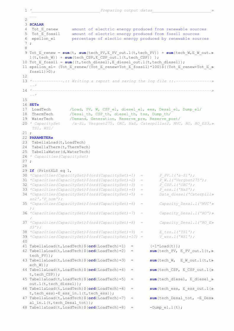
1 *_____________________________Preparing output datas_________________________»
___
2
3 SCALAR
4 T o t _ E _ r e n e w amount of electric energy produced from renewable sources
5 T o t _ E _ f o s s i l amount of electric energy produced from fossil sources
6 e p s i l o n _ e l percentage of electic energy produced by renewable sources
7 ;
8
9 Tot_E_renew = sum(t, sum(tech_PV,E_PV_out.l(t,tech_PV)) + sum(tech_W,E_W_out.»
l(t,tech_W)) + sum(tech_CSP,E_CSP_out.l(t,tech_CSP)) );
1 0 Tot_E_fossil = sum((t,tech_diesel),E_diesel_out.l(t,tech_diesel));
1 1 epsilon_el= (Tot_E_renew/(Tot_E_renew+Tot_E_fossil)*100)$((Tot_E_renew+Tot_E_»
fossil)>0);
1 2
1 3 *-------------.:: Writing a report and saving the log file ::.---------------»
--*
1 4 *----------------------------------------------------------------------------»
--*
1 5
1 6 SETs
1 7 L o a d T e c h /Load, PV, W, CSP_el, diesel_el, ees, Desal_el, Dump_el/
1 8 T h e r m T e c h /Desal_th, CSP_th, diesel_th, tss, Dump_th/
1 9 W a t e r T e c h /Demand, Generation, Reserve_pre, Reserve_post/
2 0 * CapacitySet /a-Si, Vergnet275, ORC, NaS, Caterpillar2, MVC, RO, RO_ES3,»
TS1, WS1/
2 1 ;
2 2 PARAMETERs
2 3 TabellaLoad(t,LoadTech)
2 4 TabellaTherm(t,ThermTech)
2 5 TabellaWater(d,WaterTech)
2 6 * Capacities(CapacitySet)
2 7 ;
2 8
2 9 If (PrintXLS eq 1,
3 0 *Capacities(CapacitySet)$(ord(CapacitySet)=1) = P_PV.l('a-Si');
3 1 *Capacities(CapacitySet)$(ord(CapacitySet)=2) = P_W.l('Vergnet275');
3 2 *Capacities(CapacitySet)$(ord(CapacitySet)=3) = P_CSP.l('ORC');
3 3 *Capacities(CapacitySet)$(ord(CapacitySet)=4) = P_ess.l('NaS');
3 4 *Capacities(CapacitySet)$(ord(CapacitySet)=5) = Data_diesel('Caterpill»
ar2','P_nom');
3 5 *Capacities(CapacitySet)$(ord(CapacitySet)=6) = Capacity_Desal.l('MVC'»
);
3 6 *Capacities(CapacitySet)$(ord(CapacitySet)=7) = Capacity_Desal.l('RO')»
;
3 7 *Capacities(CapacitySet)$(ord(CapacitySet)=8) = Capacity_Desal.l('RO_E»
S3');
3 8 *Capacities(CapacitySet)$(ord(CapacitySet)=9) = E_tss.l('TS1');
3 9 *Capacities(CapacitySet)$(ord(CapacitySet)=10) = V_wss.l('WS1');
4 0
4 1 TabellaLoad(t,LoadTech)$(ord(LoadTech)=1) = (-1*Load(t));
4 2 TabellaLoad(t,LoadTech)$(ord(LoadTech)=2) = sum(tech_PV, E_PV_out.l(t,»
tech_PV));
4 3 TabellaLoad(t,LoadTech)$(ord(LoadTech)=3) = sum(tech_W, E_W_out.l(t,t»
ech_W));
4 4 TabellaLoad(t,LoadTech)$(ord(LoadTech)=4) = sum(tech_CSP, E_CSP_out.l(»
t,tech_CSP));
4 5 TabellaLoad(t,LoadTech)$(ord(LoadTech)=5) = sum(tech_diesel, E_diesel_»
out.l(t,tech_diesel));
4 6 TabellaLoad(t,LoadTech)$(ord(LoadTech)=6) = sum(tech_ess, E_ess_out.l(»
t,tech_ess)-E_ess_in.l(t,tech_ess));
4 7 TabellaLoad(t,LoadTech)$(ord(LoadTech)=7) = sum(tech_Desal_tot, -E_Des»
al_in.l(t,tech_Desal_tot));
4 8 TabellaLoad(t,LoadTech)$(ord(LoadTech)=8) = -Dump_el.l(t);
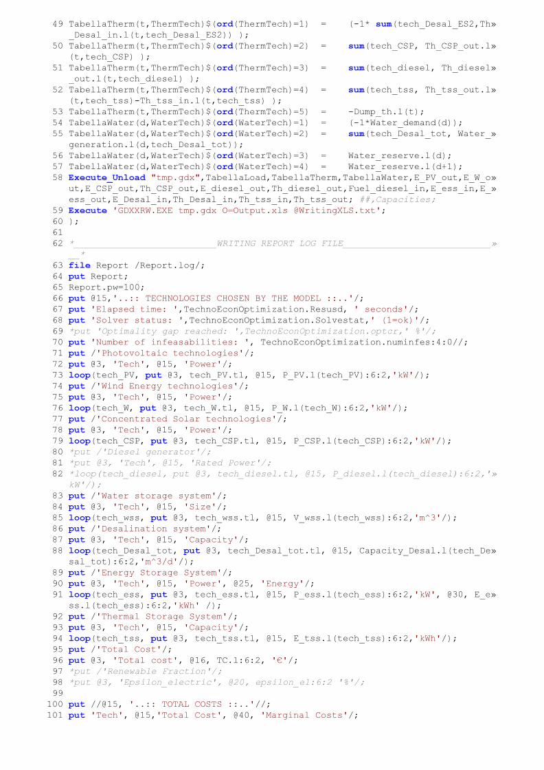
4 9 TabellaTherm(t,ThermTech)$(ord(ThermTech)=1) = (-1* sum(tech_Desal_ES2,Th»
_Desal_in.l(t,tech_Desal_ES2)) );
5 0 TabellaTherm(t,ThermTech)$(ord(ThermTech)=2) = sum(tech_CSP, Th_CSP_out.l»
(t,tech_CSP) );
5 1 TabellaTherm(t,ThermTech)$(ord(ThermTech)=3) = sum(tech_diesel, Th_diesel»
_out.l(t,tech_diesel) );
5 2 TabellaTherm(t,ThermTech)$(ord(ThermTech)=4) = sum(tech_tss, Th_tss_out.l»
(t,tech_tss)-Th_tss_in.l(t,tech_tss) );
5 3 TabellaTherm(t,ThermTech)$(ord(ThermTech)=5) = -Dump_th.l(t);
5 4 TabellaWater(d,WaterTech)$(ord(WaterTech)=1) = (-1*Water_demand(d));
5 5 TabellaWater(d,WaterTech)$(ord(WaterTech)=2) = sum(tech_Desal_tot, Water_»
generation.l(d,tech_Desal_tot));
5 6 TabellaWater(d,WaterTech)$(ord(WaterTech)=3) = Water_reserve.l(d);
5 7 TabellaWater(d,WaterTech)$(ord(WaterTech)=4) = Water_reserve.l(d+1);
5 8 Execute_Unload "tmp.gdx",TabellaLoad,TabellaTherm,TabellaWater,E_PV_out,E_W_o»
ut,E_CSP_out,Th_CSP_out,E_diesel_out,Th_diesel_out,Fuel_diesel_in,E_ess_in,E_»
ess_out,E_Desal_in,Th_Desal_in,Th_tss_in,Th_tss_out; ##,Capacities;
5 9 Execute 'GDXXRW.EXE tmp.gdx O=Output.xls @WritingXLS.txt';
6 0 );
6 1
6 2 *__________________________WRITING REPORT LOG FILE___________________________»
__*
6 3 file Report /Report.log/;
6 4 put Report;
6 5 Report.pw=100;
6 6 put @15,'..:: TECHNOLOGIES CHOSEN BY THE MODEL ::..'/;
6 7 put 'Elapsed time: ',TechnoEconOptimization.Resusd, ' seconds'/;
6 8 put 'Solver status: ',TechnoEconOptimization.Solvestat,' (1=ok)'/;
6 9 *put 'Optimality gap reached: ',TechnoEconOptimization.optcr,' %'/;
7 0 put 'Number of infeasabilities: ', TechnoEconOptimization.numinfes:4:0//;
7 1 put /'Photovoltaic technologies'/;
7 2 put @3, 'Tech', @15, 'Power'/;
7 3 loop(tech_PV, put @3, tech_PV.tl, @15, P_PV.l(tech_PV):6:2,'kW'/);
7 4 put /'Wind Energy technologies'/;
7 5 put @3, 'Tech', @15, 'Power'/;
7 6 loop(tech_W, put @3, tech_W.tl, @15, P_W.l(tech_W):6:2,'kW'/);
7 7 put /'Concentrated Solar technologies'/;
7 8 put @3, 'Tech', @15, 'Power'/;
7 9 loop(tech_CSP, put @3, tech_CSP.tl, @15, P_CSP.l(tech_CSP):6:2,'kW'/);
8 0 *put /'Diesel generator'/;
8 1 *put @3, 'Tech', @15, 'Rated Power'/;
8 2 *loop(tech_diesel, put @3, tech_diesel.tl, @15, P_diesel.l(tech_diesel):6:2,'»
kW'/);
8 3 put /'Water storage system'/;
8 4 put @3, 'Tech', @15, 'Size'/;
8 5 loop(tech_wss, put @3, tech_wss.tl, @15, V_wss.l(tech_wss):6:2,'m^3'/);
8 6 put /'Desalination system'/;
8 7 put @3, 'Tech', @15, 'Capacity'/;
8 8 loop(tech_Desal_tot, put @3, tech_Desal_tot.tl, @15, Capacity_Desal.l(tech_De»
sal_tot):6:2,'m^3/d'/);
8 9 put /'Energy Storage System'/;
9 0 put @3, 'Tech', @15, 'Power', @25, 'Energy'/;
9 1 loop(tech_ess, put @3, tech_ess.tl, @15, P_ess.l(tech_ess):6:2,'kW', @30, E_e»
ss.l(tech_ess):6:2,'kWh' /);
9 2 put /'Thermal Storage System'/;
9 3 put @3, 'Tech', @15, 'Capacity'/;
9 4 loop(tech_tss, put @3, tech_tss.tl, @15, E_tss.l(tech_tss):6:2,'kWh'/);
9 5 put /'Total Cost'/;
9 6 put @3, 'Total cost', @16, TC.l:6:2, '€'/;
9 7 *put /'Renewable Fraction'/;
9 8 *put @3, 'Epsilon_electric', @20, epsilon_el:6:2 '%'/;
9 9
1 0 0 put //@15, '..:: TOTAL COSTS ::..'//;
1 0 1 put 'Tech', @15,'Total Cost', @40, 'Marginal Costs'/;
1 0 2 loop(tech_PV, put tech_PV.tl, @15, TC_PV.l(tech_PV), '€', @35, P_PV.m(tech_»
PV):8:2, '€'/);
1 0 3 loop(tech_W, put tech_W.tl, @15, TC_W.l(tech_W), '€', @35, P_W.m(tech_W):8:»
2, '€'/);
1 0 4 loop(tech_CSP, put tech_CSP.tl, @15, TC_CSP.l(tech_CSP), '€', @35, P_CSP.m(»
tech_CSP):8:2, '€'/);
1 0 5 loop(tech_ess, put tech_ess.tl, @15, TC_ess.l(tech_ess), '€', @35, P_ess.m(»
tech_ess):8:2, '€ (P)', @50, P_ess.m(tech_ess):8:2, '€ (E)'/); ##ESS
1 0 6 *loop(tech_diesel, put tech_diesel.tl, @15, TC_diesel.l(tech_diesel), '€', @»
35, P_diesel.m(tech_diesel):8:2, '€'/);
1 0 7 loop(tech_Desal_tot, put tech_Desal_tot.tl, @15, TC_Desal.l(tech_Desal_tot),»
'€', @35, Capacity_Desal.m(tech_Desal_tot):8:2, '€'/);
1 0 8 loop(tech_wss, put tech_wss.tl, @15, TC_wss.l(tech_wss), '€', @35, V_wss.m(»
tech_wss):8:2, '€'/);
1 0 9 put '------------------------------'/;
1 1 0 put 'Total', @15, TC.l, '€'/;
1 1 1 putclose Report;
1 1 2
1 1 3
1 1 4
1 1 5
1 1 6 *__________________________COSTS REPORT LOG FILE_____________________________»
*
1 1 7 file CostReport /CostReport.log/;
1 1 8 put CostReport;
1 1 9 CostReport.pw=120;
1 2 0 put @15, '..:: ECONOMIC ANALISYS ::..'//;
1 2 1 put @4, 'Tech', @16,'IC', @28, 'O&M', @40, 'Land', @52, 'Fuel', @64, 'CO2', @»
76, 'Replac.', @88, 'Resources', @100, 'Total'/;
1 2 2
1 2 3 loop(tech_PV, put tech_PV.tl, @12, (Data_PV(tech_PV,'c_P')*P_PV.l(tech_PV)):8»
:0,'€',
1 2 4 @24, (Data_PV(tech_PV,'c_P')*P_PV.l(tech_PV)*Da»
ta_PV(tech_PV,'M_om')*Act_factor):8:0,'€',
1 2 5 @36, (c_land*P_PV.l(tech_PV)/Data_PV(tech_PV,'e»
ta')*1.5):8:0, '€',
1 2 6 @84, (P_PV.l(tech_PV)*Data_PV(tech_PV,"Resource»
s")):8:0, '€',
1 2 7 @100, TC_PV.l(tech_PV):8:0, '€'
1 2 8 /);
1 2 9 loop(tech_W, put tech_W.tl, @12, (Data_W(tech_W,'c_P')*P_W.l(tech_W)):8:0, '»
€',
1 3 0 @24, (Data_W(tech_W,'c_P')*P_W.l(tech_W)*Data_W(»
tech_W,'M_om')*Act_factor):8:0, '€',
1 3 1 @36, (c_land*Data_W(tech_W,'land_use')*P_W.l(tec»
h_W)):8:0, '€',
1 3 2 @84, (P_W.l(tech_W)*Data_W(tech_W,"Resources")):»
8:0, '€',
1 3 3 @100, TC_W.l(tech_W):8:0, '€'
1 3 4 /);
1 3 5 loop(tech_CSP, put tech_CSP.tl, @12, (Data_CSP(tech_CSP,'c_P')*P_CSP.l(tech_»
CSP)):8:0, '€',
1 3 6 @24, (Data_CSP(tech_CSP,"M_om")*P_CSP.l(tech»
_CSP)*Act_factor):8:0, '€',
1 3 7 @36, (c_land*Data_CSP(tech_CSP,'land_use')*P»
_CSP.l(tech_CSP)):8:0, '€',
1 3 8 @84, (P_CSP.l(tech_CSP)*Data_CSP(tech_CSP,"R»
esources")):8:0, '€',
1 3 9 @100, TC_CSP.l(tech_CSP):8:0, '€'
1 4 0 /);
1 4 1 loop(tech_diesel, put tech_diesel.tl, @12, (Data_diesel(tech_diesel,'c_P')*D»
ata_diesel(tech_diesel,'P_nom')):8:0, '€',
1 4 2 @24, (Data_diesel(tech_diesel,'c_om')*»
Act_factor *sum(t,E_diesel_out.l(t,tech_diesel))):8:0, '€',
1 4 3 @36, (c_land*Data_diesel(tech_diesel,'»
land_use')*Data_diesel(tech_diesel,'P_nom')):8:0, '€',
1 4 4 @48, (c_diesel * Act_factor * sum(t,Fu»
el_diesel_in.l(t,tech_diesel))):8:0, '€',
1 4 5 @60, (c_CO2*CO2_from_diesel * Act_fact»
or * sum(t,Fuel_diesel_in.l(t,tech_diesel))):8:0, '€',
1 4 6 @84, (Data_diesel(tech_diesel,"P_nom")»
*Data_diesel(tech_diesel,"Resources")):8:0, '€',
1 4 7 @100, TC_diesel.l(tech_diesel):8:0, '€'
1 4 8 /);
1 4 9 loop(tech_Desal_tot, put tech_Desal_tot.tl, @12, (Data_Desal(tech_Desal_tot,»
'c_plant')*Capacity_Desal.l(tech_Desal_tot)):8:0, '€',
1 5 0 @24, (Data_Desal(tech_Desal_tot,'c_om') »
* Act_factor * sum(d,Water_generation.l(d,tech_Desal_tot))):8:0, '€',
1 5 1 @36, (c_land*Data_Desal(tech_Desal_tot,"»
land_use")*Capacity_Desal.l(tech_Desal_tot)):8:0, '€',
1 5 2 @84, (Capacity_Desal.l(tech_Desal_tot)*D»
ata_Desal(tech_Desal_tot,"Resources")):8:0, '€',
1 5 3 @100, TC_Desal.l(tech_Desal_tot):8:0, '€'
1 5 4 /);
1 5 5 loop(tech_ess, put tech_ess.tl, @12, (Data_ess(tech_ess,'c_P')*P_ess.l(tech_»
ess)+Data_ess(tech_ess,'c_E')*E_ess.l(tech_ess)):8:0, '€',
1 5 6 @24, (Data_ess(tech_ess,'OandM')*P_ess.l(tec»
h_ess)*Act_factor):8:0, '€',
1 5 7 @36, (c_land*Data_ess(tech_ess,'land_use')*E»
_ess.l(tech_ess)):8:0, '€',
1 5 8 @48, (c_fuel*Data_ess(tech_ess,'fuel_cons')*»
Act_factor* sum(t,E_ess_out.l(t,tech_ess))):8:0, '€',
1 5 9 @60, (c_CO2*CO2_from_fuel*Data_ess(tech_ess,»
'fuel_cons')*Act_factor*sum(t,E_ess_out.l(t,tech_ess))):8:0, '€',
1 6 0 @72, ((Data_ess(tech_ess,'c_r_P')*P_ess.l(te»
ch_ess)+Data_ess(tech_ess,'c_r_E')*E_ess.l(tech_ess))*sum(y,((1/(1+interest_r»
ate))**ord(y))$(mod(ord(y),Data_ess(tech_ess,'life'))=0))):8:0, '€',
1 6 1 @84, (P_ess.l(tech_ess)*Data_ess(tech_ess,"R»
esources")):8:0, '€',
1 6 2 @100, TC_ess.l(tech_ess):8:0, '€'
1 6 3 /);
1 6 4 loop(tech_tss, put tech_tss.tl, @12, (Data_tss(tech_tss,'spec_cost')*E_tss.l»
(tech_tss)):8:0, '€',
1 6 5 @24, (Data_tss(tech_tss,'OandM')*E_tss.l(tec»
h_tss) * Act_factor):8:0, '€',
1 6 6 @36, (c_land*Data_tss(tech_tss,'land_use')*E»
_tss.l(tech_tss)):8:0, '€',
1 6 7 @84, (E_tss.l(tech_tss)*Data_tss(tech_tss,"R»
esources")):8:0, '€',
1 6 8 @100, TC_tss.l(tech_tss):8:0, '€'
1 6 9 /);
1 7 0 loop(tech_wss, put tech_wss.tl, @12, (Data_wss(tech_wss,'spec_cost')*V_wss.l»
(tech_wss)):8:0, '€',
1 7 1 @36, (c_land*Data_wss(tech_wss,'land_use')*V»
_wss.l(tech_wss)):8:0, '€',
1 7 2 @84, (V_wss.l(tech_wss)*Data_wss(tech_wss,"R»
esources")):8:0, '€',
1 7 3 @100, TC_wss.l(tech_wss):8:0, '€'
1 7 4 /);
1 7 5
1 7 6 put '------------------------------------------------------------------------»
------------------------------------'/;
1 7 7 put 'Total', @100, TC.l:8:0, '€'/;
1 7 8 putclose CostReport;
1 7 9
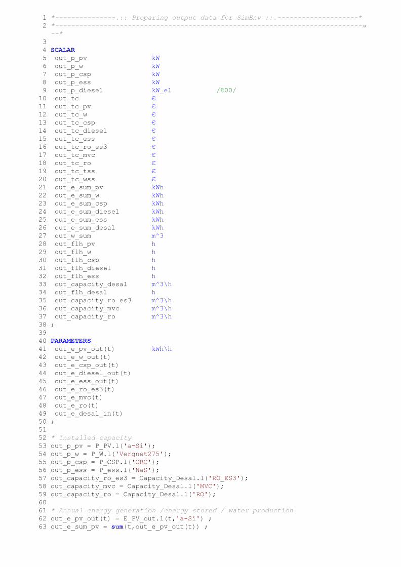
1 *---------------.:: Preparing output data for SimEnv ::.--------------------*
2 *----------------------------------------------------------------------------»
--*
3
4 SCALAR
5 o u t _ p _ p v kW
6 o u t _ p _ w kW
7 o u t _ p _ c s p kW
8 o u t _ p _ e s s kW
9 o u t _ p _ d i e s e l k W _ e l /800/
1 0 o u t _ t c €
1 1 o u t _ t c _ p v €
1 2 o u t _ t c _ w €
1 3 o u t _ t c _ c s p €
1 4 o u t _ t c _ d i e s e l €
1 5 o u t _ t c _ e s s €
1 6 o u t _ t c _ r o _ e s 3 €
1 7 o u t _ t c _ m v c €
1 8 o u t _ t c _ r o €
1 9 o u t _ t c _ t s s €
2 0 o u t _ t c _ w s s €
2 1 o u t _ e _ s u m _ p v kWh
2 2 o u t _ e _ s u m _ w kWh
2 3 o u t _ e _ s u m _ c s p kWh
2 4 o u t _ e _ s u m _ d i e s e l kWh
2 5 o u t _ e _ s u m _ e s s kWh
2 6 o u t _ e _ s u m _ d e s a l kWh
2 7 o u t _ w _ s u m m^3
2 8 o u t _ f l h _ p v h
2 9 o u t _ f l h _ w h
3 0 o u t _ f l h _ c s p h
3 1 o u t _ f l h _ d i e s e l h
3 2 o u t _ f l h _ e s s h
3 3 o u t _ c a p a c i t y _ d e s a l m^3\h
3 4 o u t _ f l h _ d e s a l h
3 5 o u t _ c a p a c i t y _ r o _ e s 3 m^3\h
3 6 o u t _ c a p a c i t y _ m v c m^3\h
3 7 o u t _ c a p a c i t y _ r o m^3\h
3 8 ;
3 9
4 0 PARAMETERS
4 1 out_e_pv_out(t) kWh\h
4 2 out_e_w_out(t)
4 3 out_e_csp_out(t)
4 4 out_e_diesel_out(t)
4 5 out_e_ess_out(t)
4 6 out_e_ro_es3(t)
4 7 out_e_mvc(t)
4 8 out_e_ro(t)
4 9 out_e_desal_in(t)
5 0 ;
5 1
5 2 * Installed capacity
5 3 out_p_pv = P_PV.l('a-Si');
5 4 out_p_w = P_W.l('Vergnet275');
5 5 out_p_csp = P_CSP.l('ORC');
5 6 out_p_ess = P_ess.l('NaS');
5 7 out_capacity_ro_es3 = Capacity_Desal.l('RO_ES3');
5 8 out_capacity_mvc = Capacity_Desal.l('MVC');
5 9 out_capacity_ro = Capacity_Desal.l('RO');
6 0
6 1 * Annual energy generation /energy stored / water production
6 2 out_e_pv_out(t) = E_PV_out.l(t,'a-Si') ;
6 3 out_e_sum_pv = sum(t,out_e_pv_out(t)) ;
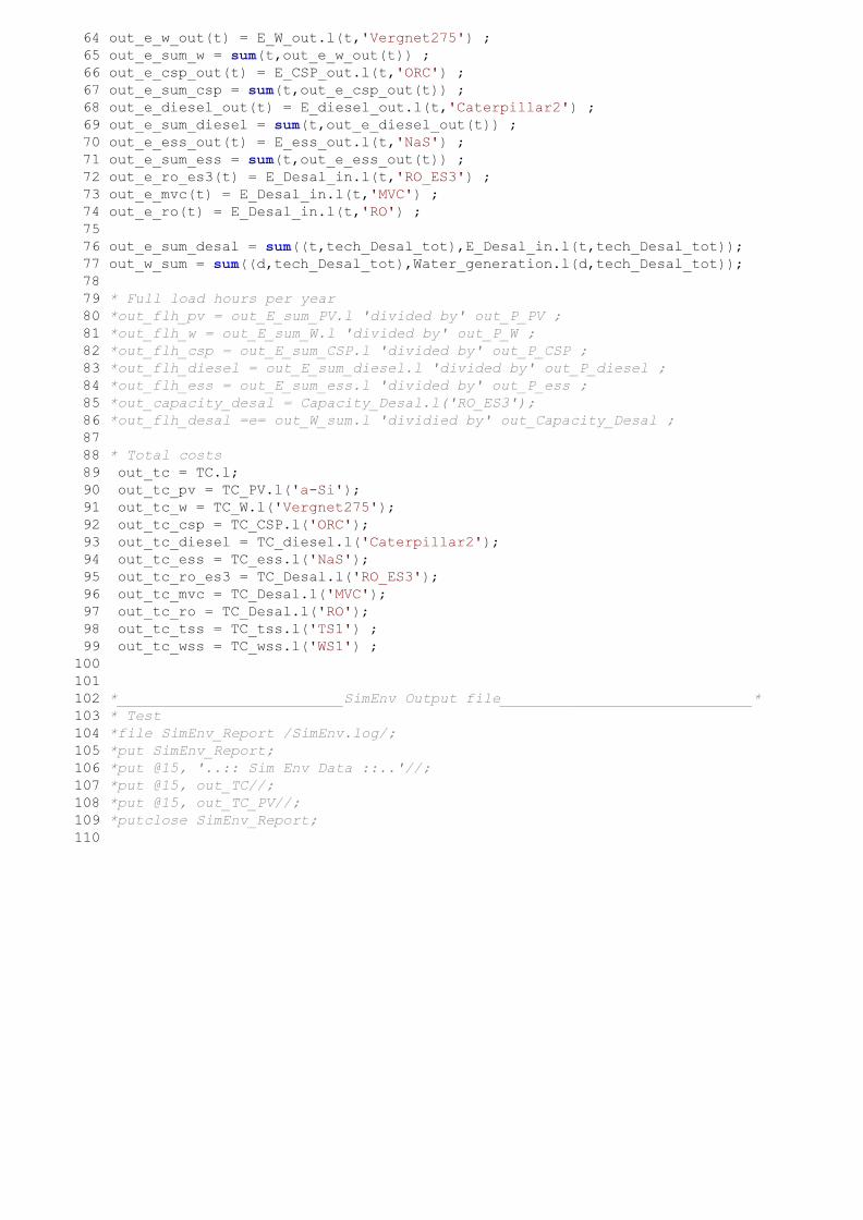
6 4 out_e_w_out(t) = E_W_out.l(t,'Vergnet275') ;
6 5 out_e_sum_w = sum(t,out_e_w_out(t)) ;
6 6 out_e_csp_out(t) = E_CSP_out.l(t,'ORC') ;
6 7 out_e_sum_csp = sum(t,out_e_csp_out(t)) ;
6 8 out_e_diesel_out(t) = E_diesel_out.l(t,'Caterpillar2') ;
6 9 out_e_sum_diesel = sum(t,out_e_diesel_out(t)) ;
7 0 out_e_ess_out(t) = E_ess_out.l(t,'NaS') ;
7 1 out_e_sum_ess = sum(t,out_e_ess_out(t)) ;
7 2 out_e_ro_es3(t) = E_Desal_in.l(t,'RO_ES3') ;
7 3 out_e_mvc(t) = E_Desal_in.l(t,'MVC') ;
7 4 out_e_ro(t) = E_Desal_in.l(t,'RO') ;
7 5
7 6 out_e_sum_desal = sum((t,tech_Desal_tot),E_Desal_in.l(t,tech_Desal_tot));
7 7 out_w_sum = sum((d,tech_Desal_tot),Water_generation.l(d,tech_Desal_tot));
7 8
7 9 * Full load hours per year
8 0 *out_flh_pv = out_E_sum_PV.l 'divided by' out_P_PV ;
8 1 *out_flh_w = out_E_sum_W.l 'divided by' out_P_W ;
8 2 *out_flh_csp = out_E_sum_CSP.l 'divided by' out_P_CSP ;
8 3 *out_flh_diesel = out_E_sum_diesel.l 'divided by' out_P_diesel ;
8 4 *out_flh_ess = out_E_sum_ess.l 'divided by' out_P_ess ;
8 5 *out_capacity_desal = Capacity_Desal.l('RO_ES3');
8 6 *out_flh_desal =e= out_W_sum.l 'dividied by' out_Capacity_Desal ;
8 7
8 8 * Total costs
8 9 out_tc = TC.l;
9 0 out_tc_pv = TC_PV.l('a-Si');
9 1 out_tc_w = TC_W.l('Vergnet275');
9 2 out_tc_csp = TC_CSP.l('ORC');
9 3 out_tc_diesel = TC_diesel.l('Caterpillar2');
9 4 out_tc_ess = TC_ess.l('NaS');
9 5 out_tc_ro_es3 = TC_Desal.l('RO_ES3');
9 6 out_tc_mvc = TC_Desal.l('MVC');
9 7 out_tc_ro = TC_Desal.l('RO');
9 8 out_tc_tss = TC_tss.l('TS1') ;
9 9 out_tc_wss = TC_wss.l('WS1') ;
1 0 0
1 0 1
1 0 2 *__________________________SimEnv Output file_____________________________*
1 0 3 * Test
1 0 4 *file SimEnv_Report /SimEnv.log/;
1 0 5 *put SimEnv_Report;
1 0 6 *put @15, '..:: Sim Env Data ::..'//;
1 0 7 *put @15, out_TC//;
1 0 8 *put @15, out_TC_PV//;
1 0 9 *putclose SimEnv_Report;
1 1 0
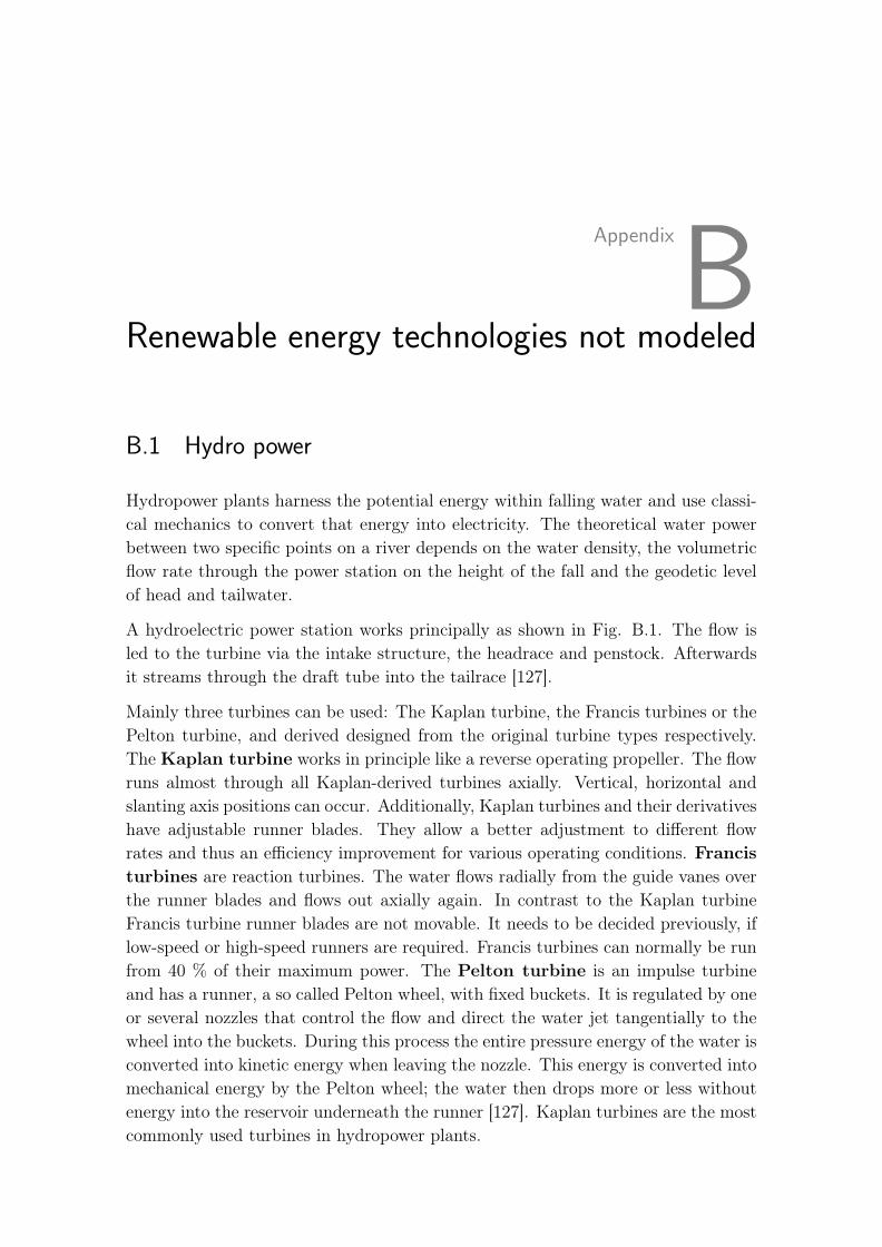
Appendix
BRenewable energy technologies not modeled
B.1 Hydro power
Hydropower plants harness the potential energy within falling water and use classi-cal mechanics to convert that energy into electricity. The theoretical water powerbetween two specific points on a river depends on the water density, the volumetricflow rate through the power station on the height of the fall and the geodetic levelof head and tailwater.
A hydroelectric power station works principally as shown in Fig. B.1. The flow isled to the turbine via the intake structure, the headrace and penstock. Afterwardsit streams through the draft tube into the tailrace [127].
Mainly three turbines can be used: The Kaplan turbine, the Francis turbines or thePelton turbine, and derived designed from the original turbine types respectively.The Kaplan turbine works in principle like a reverse operating propeller. The flowruns almost through all Kaplan-derived turbines axially. Vertical, horizontal andslanting axis positions can occur. Additionally, Kaplan turbines and their derivativeshave adjustable runner blades. They allow a better adjustment to different flowrates and thus an efficiency improvement for various operating conditions. Francisturbines are reaction turbines. The water flows radially from the guide vanes overthe runner blades and flows out axially again. In contrast to the Kaplan turbineFrancis turbine runner blades are not movable. It needs to be decided previously, iflow-speed or high-speed runners are required. Francis turbines can normally be runfrom 40 % of their maximum power. The Pelton turbine is an impulse turbineand has a runner, a so called Pelton wheel, with fixed buckets. It is regulated by oneor several nozzles that control the flow and direct the water jet tangentially to thewheel into the buckets. During this process the entire pressure energy of the water isconverted into kinetic energy when leaving the nozzle. This energy is converted intomechanical energy by the Pelton wheel; the water then drops more or less withoutenergy into the reservoir underneath the runner [127]. Kaplan turbines are the mostcommonly used turbines in hydropower plants.
186 Chapter B Renewable energy technologies not modeled
Fig. B.1: Physical correlations in a hydroelectric power station [127]
B.2 Ocean powers
Ocean energy has many forms: tides, surface waves, ocean circulation, salinity, andthermal gradients. The ocean offers a lot of intriguing energy sources. Since someplants can also be implemented in the range of one megawatt, the state-of-the-artof some oceanic power generators will be addressed briefly.
Wave powerWind-driven waves derive ultimately from solar energy. Because of its considerableenergy potential, for several decades wave energy has been investigated with regardto power generation. Waves of the height of two meters and a period of six secondsfor example, as typical for the German North Sea coast, could theoretically generateapproximately 14 kW/m and 3.6 GW in a coast length of about 250 km[128]. Onlyfor using wave energy various technologies have been developed: tapered channelsystems, float systems, oscillating water column systems, underwater turbines etc.Similar to hydroelectric dams, channel systems raise the intake water higher thansea level and let the water run down through a turbine. Float systems lay on the seasurface and waves run hydraulic pumps or pistons that power a turbine. Oscillatingwater column systems let waves enter a chamber to push air up with the same goal,to power a turbine. Underwater turbines work like wind mills. Instead of windthough, they use the water current to turn the blades in the ocean. The mostcommon energy capture methods are surface-following attenuators and oscillatingwater column buoys. The most recent plants were built and are still planned inthe United Kingdom, Australia, Belgium, Korea and China [129]. Up to now veryfew facilities of wave energy conversion to electricity operate commercially. Mostof them are publicly funded pilot plants. For economical reasons they were notcommercialized yet. Wave energy converters though could combine power generationand coastline protection (since kinetic energy is taken from the waves) and enhancethe economic attractiveness of wave energy exploitation [128].
B.2 Ocean powers 187
Tidal EnergyDriven by gravitational effects the ocean level rises and falls. Marine currents arepredictable and the change of the sea level can be exploited. Tides can be usedin two different ways for power generation: The potential energy of backwaters ormarine currents can be used by tidal power stations.
The first one works similar to the hydroelectric dam generation method, filling abay with seawater and releasing it through turbine systems. Its advantage is thesimple turbine design, its disadvantage though the relatively short time period inwhich electricity can be generated. Tidal power stations can also be designed as atwo-basin system, but are more demanding and the two basins require more space.The exploitation method based on the high and low tide stream, and thus on watermotion caused by low and high tides faces the challenge of relatively low energydensities. Savonius or Darrieus rotors are used for these slow current speeds. Up tonow, first prototypes are in operation, but projects of pure high and low tide streamexploitation have not been put into practice yet.
A tidal energy facility performs most effective, if the minimum tidal level differencebetween high and low tide is approximately 5 meters. Not many areas of the oceansmeet this requirement, therefore only few applications were implemented until now[129]. The largest tidal energy facility is at La Rance in France and has beenin operation since 1967. It has a capacity of 180 million m3 with a tidal range ofapproximately 8.5 meters and an installed capacity of 240 MW, producing 600 GWha year. This amount supplies enough energy for 250,000 households. Another smallerfacility with a capacity of 20 MW is located in Annapolis Royer, Canada, producing30 GWh yearly. The third tidal energy plant is at Kislaya Guba in Russia with0.5 MW capacity. Two further plants were constructed in China. An economicalbreakthrough could not be achieved yet [128].
Thermal gradient Ocean Thermal Energy Conversion (OTEC) is based on drivinga power conversion cycle by the temperature difference between surface seawaterand seawater at a depth of around 1000 meters or even more. In principle, thistype of thermal energy could be used for power generation by means of open orclosed Rankine processes. The warm seawater flashes in a low pressure or vacuumchamber, where after expansion it condenses through a heat exchanger, cooled bysurrounding seawater. The water temperature difference ranges from a maximumof 22 to approximately 28 ◦C and the cold deep waters of approximately 4 to 7 ◦C.These power plants can only achieve very low efficiencies of under 5 % [128]. Researchis in progress but up to date, no system has been implemented yet. Its commercialdevelopment is limited due to economic aspects.
A combination of this technology with geothermal power plants, increasing the tem-perature differences between warm areas near volcanic structures and cold oceanwater are conceivable. However, it is unlikely that this method will be put intopractice in the near future due to considerable technical problems.
188 Chapter B Renewable energy technologies not modeled
B.3 Geothermal energy
Compared to fluctuating solar, wind or oceanic energy, geothermal energy is ableto assure a constant energy supply, making it applicable as source for base load.Geothermal energy is thermal energy stored in high-pressure water zones, steam, orhot stones below the earth’s surface. It consists partly of the permanent heat flowfrom the earth’s core (about 30 %); the other part originates from natural radioac-tive decay processes taking place in the mantle. Near to the surface geothermalenergy can supply buildings with heat and warm water by earth heat collectors incombination with heat pumps in a depth of approximately 15 to 150 meters. Thetemperature in the earth’s mantle increases by around 3 ◦C every 100 meter depths[130].
For generating electricity in a direct way geothermal reservoirs above 130 ◦C arerequired. Volcanic regions or layers in great depth from 2000 to 5000 meters needusually to be found. The "coldest" geothermal power plant of the world is locatedin Germany (Neustadt-Glewe), operating at a temperature of approximately 98 ◦C.The provision of electrical energy is possible but not efficient. Currently the plant isnot in operation. Geothermal energy of temperatures above 150 ◦C is currently usedespecially in Iceland, New Zealand and Italy [131]. The first geothermal power plantwas built in 1904 in Tuscany, Italy at a place where natural steam was erupting fromthe earth.
There are different methods of collecting geothermal energy: the fluid-dominated,the vapour (steam)-dominated and the Hot-Dry-Rock (HDR) process. At the fluid-dominated system high-pressure hot water is transported through wells from deepinside the earth and converted/flashed into steam. If steam itself is found in ageothermal reservoir, it is used directly to turn generator turbines in so called drysteam plants. When the steam cools, it condenses to water and is injected backinto the ground to be used over and over again. The Hot-Dry-Rock method workssimilar: Wells are drilled into the granite layer, which has temperatures over 200 ◦C.Through one of the wells water is injected down into the granite layer where it isheated. The hot water returns back to the surface through another well, where it iskept under pressure and therefore in liquid form, in order to run a turbine system.Most geothermal power plants are flash plants. Binary power plants transfer heatfrom geothermal hot water to another liquid. The heat causes the second liquid toturn to steam, which is used to drive a generator turbine. Today production ratesup to 10 MW of thermal energy are common [131].
Although in the past approaches have been done to implement slim holes for smalloff-grid power generation [132] they could not be asserted. Geothermal power plantscan only operate effectively and beneficial as large-scale applications. Especially theexpensive drillings in the preparation-phase increase costs tremendously, becauseit is not secure, whether or not the required sediment or hydrothermal conditions
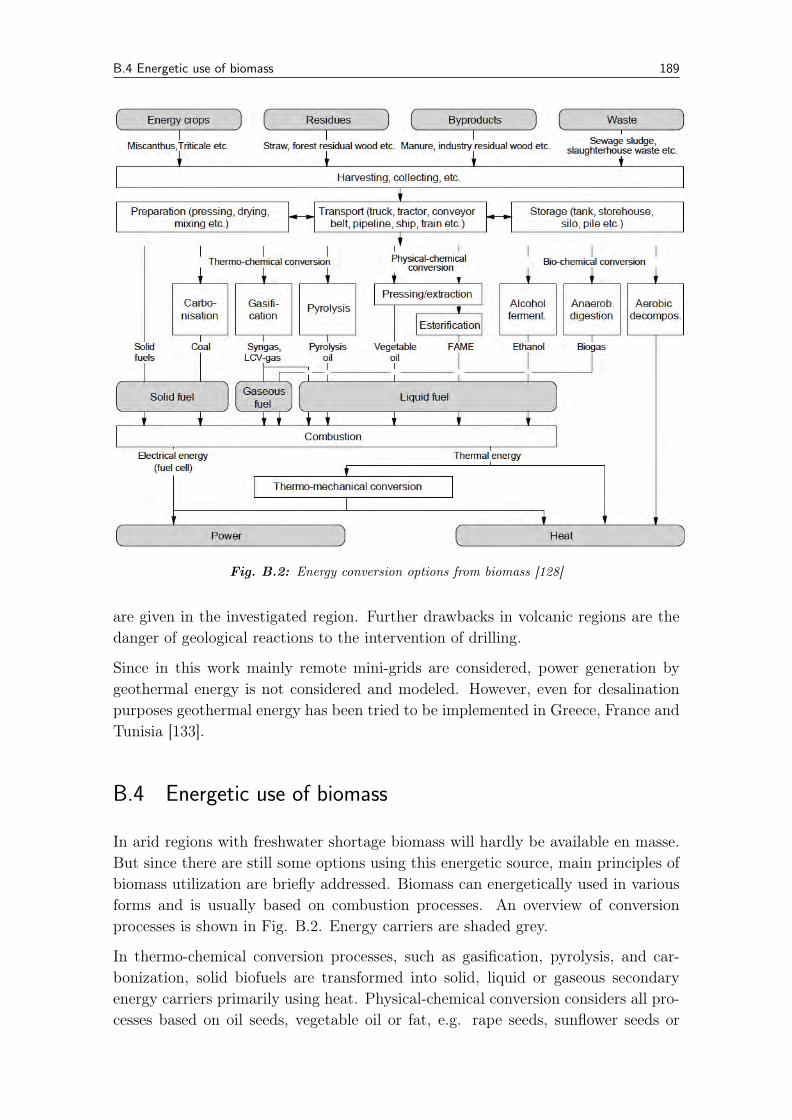
B.4 Energetic use of biomass 189
Fig. B.2: Energy conversion options from biomass [128]
are given in the investigated region. Further drawbacks in volcanic regions are thedanger of geological reactions to the intervention of drilling.
Since in this work mainly remote mini-grids are considered, power generation bygeothermal energy is not considered and modeled. However, even for desalinationpurposes geothermal energy has been tried to be implemented in Greece, France andTunisia [133].
B.4 Energetic use of biomass
In arid regions with freshwater shortage biomass will hardly be available en masse.But since there are still some options using this energetic source, main principles ofbiomass utilization are briefly addressed. Biomass can energetically used in variousforms and is usually based on combustion processes. An overview of conversionprocesses is shown in Fig. B.2. Energy carriers are shaded grey.
In thermo-chemical conversion processes, such as gasification, pyrolysis, and car-bonization, solid biofuels are transformed into solid, liquid or gaseous secondaryenergy carriers primarily using heat. Physical-chemical conversion considers all pro-cesses based on oil seeds, vegetable oil or fat, e.g. rape seeds, sunflower seeds or
190 Chapter B Renewable energy technologies not modeled
coconuts. Running through a number of separation and conversion steps, the ob-tained vegetable oil can be used as a fuel for engines and CHP plants and is ap-plied either in its pure form or after chemical conversion to Fatty Acid Methyl Ester(FAME). Bio-chemical processes use micro-organisms or bacteria to convert biomassinto secondary energy carriers or useful energy. Fermentation into alcohol, aerobicfermentation and aerobic digestion are such bio-chemical processes. The most com-mon process used in remote regions is the anaerobic digestion with biogas as finalproduct [128, 134].
The identification of applicable processes depends highly on the biomass potential inthe considered region. A collection of biomass potentials in Small Island DevelopingStates is listed in Fig. B.3. The dark marked arrays stand for high potentials, lightmarked arrays for low or no potential.
Only secondary or tertiary biomass is considered. The potentials are divided intobiomass from forestry, agriculture, animal husbandry, tourism and organic waste.
As mentioned before, remote regions with freshwater scarcity will hardly have largeamounts of surplus biomass. Some dry regions though have a good potential ofgrowing specific energy plants, whose oil can supplement diesel fuel with biofuel,such as canola, oil palm, soy or jatropha. Jatropha curcas is one of the few droughtresistant and perennial oil plants. It is a tropical plant that can be grown in dry andhumid areas. The soil conditions should be around pH 4.5. The plants have a usefullife of about 30 years and have a 30 % oil content in their seeds. Annually two to fourtons per hectare of the oily nut seeds can be harvested, resulting in approximately upto 4000 to 8000 litres biofuel. Biodiesel can be produced by extraction of the seedswith an oil mill. The properties of jatropha curcas oil are a density of 884 kg/m3
(at 15 ◦C), a phosphorus and sulphur content of less than 1 mg/kg and a cetanenumber of 60, which is a relatively high and good with respect to its usability inengines (rape oil 54) [135].
A further approach growing biomass is to use algae. Algae are an attractive wayto harvest solar energy and turn carbon dioxide into biofuel. A lot of resourcesare thus being put into the idea of turning algae into mini oil wells. Algae cangrow in salt water, freshwater or even in contaminated water at sea or in ponds.But the challenges are many. Algae use carbon dioxide to produce oil moleculesvia photosynthesis. The greatest challenge of algal biofuel is the production of oilon a much larger scale but at much lower costs. As per one estimate the scale ofproduction needs to increase at least three orders of magnitude, with a decrease in thecost of production by a factor of ten. The main distinction between algae-conceptsis the cultivation system; both open pools and closed tubular reactor systems areinvestigated. Significant research results will be needed for large scale applications.Up to now a technological breakthrough is not conceivable.
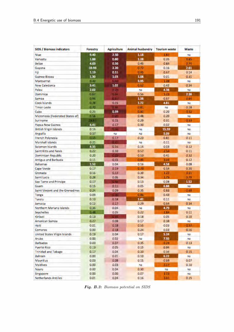
B.4 Energetic use of biomass 191
Fig. B.3: Biomass potential on SIDS
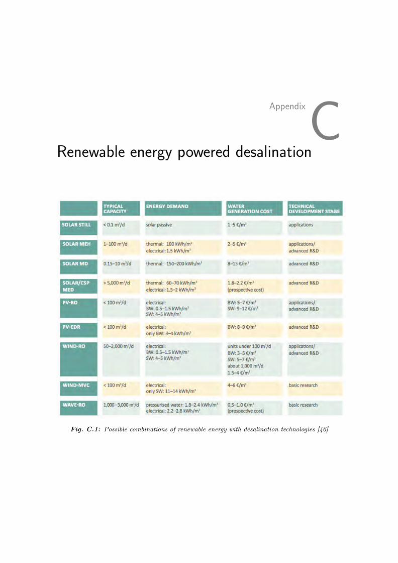
Appendix
CRenewable energy powered desalination
Fig. C.1: Possible combinations of renewable energy with desalination technologies [46]