emulated flexible manufacturing...
TRANSCRIPT

EMULATED FLEXIBLE MANUFACTURING FACILITY
By
AZIZ BATUR ALUSKAN
A THESIS PRESENTED TO THE GRADUATE SCHOOLOF THE UNIVERSITY OF FLORIDA IN PARTIAL FULFILLMENT
OF THE REQUIREMENTS FOR THE DEGREE OFMASTER OF SCIENCE
UNIVERSITY OF FLORIDA
1999

Copyright by
Aziz Batur Aluskan
1999

iii
ACKNOWLEDGMENTS
I would like to thank and acknowledge my gratefulness to my parents Gonul and Erten
Aluskan, and my sister Basak Aluskan for their never ending love and support throughout
my life. Also my sincere and deepest gratitude goes to my advisor Dr. Suleyman Tufekci,
for his true understanding, invaluable support and unique inspiration. Working with him
was a privilege that I took for granted. I would like to express my thanks to Dr. Schaub
and Dr. Bai for their feedback and constructive criticisms in completing this work.
This research was partially funded by National Science Foundation and SUCCEED
Coalition, whom I gratefully acknowledge.
I also would like to thank all my friends in the EFML Laboratory, Kursat Apan, Burak
Eksioglu, Tim Elftman, Thomas Hochreiter and Murat Yegengil. Also, I would like to
thank all the members of the Industrial and Systems Engineering Department for the very
nice atmosphere they have created.
Special thanks go to Ahmet Gokhan Guner for his lifelong friendship and support.
Last, but not the least, my sincere gratefulness to Zeynep Orhon for her priceless moral
support.

iv
TABLE OF CONTENTS
page
ACKNOWLEDGEMENTS ............................................................................................ iii
LIST OF TABLES ......................................................................................................... vi
LIST OF FIGURES....................................................................................................... vii
ABSTRACT................................................................................................................... ix
1 INTRODUCTION.......................................................................................................1
2 BACKGROUND INFORMATION .............................................................................6
2.1 Computer Simulation......................................................................................62.2 Discrete Event Simulation ..............................................................................82.3. Simulation in Manufacturing........................................................................102.4 The Concept of Virtual Factories and EFMF ................................................112.5 The EFMF Environment Architecture...........................................................132.6 Abilities of EFMF.........................................................................................15
3 GRAPHICAL USER INTERFACE AND OPERATION ...........................................17
3.1 Design Principles..........................................................................................173.2 Factory Setup Object....................................................................................183.3 Machine and Assembly Object ......................................................................283.4 Machine Wizard Objects...............................................................................333.5 Dispatch Object ............................................................................................363.6 Finished Goods Object .................................................................................403.7 Transportation Object...................................................................................423.8 Repair Object ...............................................................................................48
4 DATABASES ...........................................................................................................51
4.1 Introduction .................................................................................................514.2 Machine Library ...........................................................................................514.3 Factory Setup Object Database.....................................................................534.4 Machine and Assembly Object Database .......................................................54

v
4.5 Transportation Object Database....................................................................614.6 Finished Goods and Shipment Object Database.............................................634.7 Dispatch Object Database.............................................................................694.8 Repair Object ...............................................................................................76
5 DATABASE UTILITY TOOL ..................................................................................78
6 CONCLUSIONS.......................................................................................................84
6.1 Summary......................................................................................................846.2 Future Work.................................................................................................85
LIST OF REFERENCES...............................................................................................89
BIOGRAPHICAL SKETCH .........................................................................................90

vi
LIST OF TABLES
Table page
3.1: Color-codes for the machine object .........................................................................28
3.2 Types of edit boxes in Machine Wizard 2 .................................................................36
4.1: Machine Library, machine.db..................................................................................53
4.2: Machine library (factory.db) example. .....................................................................54
4.3: An example Setup table for a machine. ....................................................................57
4.4: Cell definitions for the setup table. ..........................................................................58
4.5: The definition for the Kanban Out field of the batch table. ......................................61
4.6: Trans.db example. ..................................................................................................62
4.7: A distances.db example. .........................................................................................63
4.8: Structure of Inset.db ...............................................................................................64
4.9: Structure of Orders.db and Osorders.db. ................................................................64
4.10: Outqueue.db .........................................................................................................64
4.11: Log1.db ................................................................................................................77
4.12: Repair.db..............................................................................................................77

vii
LIST OF FIGURES
Figure page
3.1 Factory Setup Object. ..............................................................................................19
3.2 Directory selector used for New and Save As commands. ........................................20
3.3 User interface of Stop Condition: (a) for the first two options and (b) for the lastoption. ...................................................................................................................24
3.4 Design toolbar. ........................................................................................................25
3.5 Experiment toolbar: (a) before initialization of the Kanban and CONWIP and (b) afterinitialization of the Kanban and CONWIP. .............................................................26
3.6 Termination toolbar. ................................................................................................26
3.7 Possible states. .........................................................................................................26
3.8 The user interface to access the parameter table. ......................................................27
3.9 Machine object.........................................................................................................29
3.10 Machine Wizard 1. .................................................................................................34
3.11 Machine Wizard 2. .................................................................................................34
3.12 Dispatch Object. ....................................................................................................39
3.13 The form Product Tree Constructor: (a) when adding a new product and (b) whenadding a new intermediate product or raw material (component). ..........................40
3.14 Products object. .....................................................................................................41
3.15 Transporter Object. ................................................................................................44
3.16 New Transporter object (old version). ....................................................................45
3.17 Distance Matrix .....................................................................................................45

viii
3.18 Transporter Design ................................................................................................46
3.19 DB Navigator object ..............................................................................................47
3.20 Repair object..........................................................................................................50
5.1. Database NaviGator (Mainform). ............................................................................78
5.2 The form DBaseDesigner. ........................................................................................79
5.3 The form DBNavigator at design time......................................................................80
5.4 The form DirBrowser...............................................................................................80
5.5 The form SelectWorkingDir. ....................................................................................81

ix
Abstract of Thesis Presented to the Graduate Schoolof the University of Florida in Partial Fulfillment of the
Requirements for the Degree of Master of Science
EMULATED FLEXIBLE MANUFACTURING FACILITY
By
Aziz Batur Aluskan
August 1999
Chairman: Dr. Suleyman TufekciMajor Department: Industrial and Systems Engineering
The goal of manufacturing is to improve the life of the people by creating products
that are dependable, affordable and elegant, while maintaining the highest quality and most
desired functionality. Another goal of manufacturing is to serve the purpose driving the
economy.
Today, main areas of research in manufacturing are attaining significant reductions
in manufacturing lead-time and prominent developments in matching delivery dates. Better
methods in production scheduling and planning will decrease the period of changing the
raw material and parts to finished goods, or products. In fact, real factory environment is
far from simple. In order to get a global perspective about the manufacturing facility and
how this facility would respond to the changes, manufacturing researchers have developed
countless simulation models in order to create a virtual model of the factory to emulate all
the activities that are going on.

x
Simulation can be defined as the usage of applications and methods to mimic, or
imitate the behavior of real systems, using computers and suitable software at hand. The
idea of simulation applies to many industrial and academic fields in immeasurable forms,
and with the inception of the latest developments in information technology, computers
and software are more useful than ever.
Emulated Flexible Manufacturing Facility (EFMF) is a simulation tool, where the
manufacturing facility is “built” in a virtual design environment. It is not a simulation
software; however a simulator which is specifically tailored to “emulate” the
manufacturing facility while encompassing the latest developments in the factory physics,
manufacturing and scheduling systems.
The development of EFMF is partially made possible by funding from the National
Science Foundation (NSF) and the Southeastern University and College Coalition for
Engineering Education (SUCCEED) since 1993. Windows NT are used as the operating
system and Borland Delphi 3.0 and Borland Paradox is used for application and database
utility tools respectively.

1
CHAPTER 1 INTRODUCTION
The goal of manufacturing is to make money for the company in the present as
well as in the future, and by doing so, to improve the life of the people by creating
products that are dependable, affordable and elegant, while maintaining the highest quality
and most desired functionality. A shorter description can be to meet desired customer
characteristics, quality and reliability.
Another goal of manufacturing is to serve the purpose of driving the economy.
However, the percentage of manufacturing-based employment has decreased perpetually
throughout the last century, shifting the emphasis to service industry. 1960s experienced
an economic boom, which assured that anything that is produced can essentially be sold at
a profit. As the world is turning into one big competitive marketplace, a process of
ongoing improvement is the key to a company’s survival.
According to the processing types, there are two kinds of manufacturing. The
discrete-parts manufacturing involves separate components that are clearly
distinguishable from one another. Examples include automobile tire or dining table
manufacturing. On the other hand, continuous processing manufacturing lines involve
products of steadily flowing nature. Oil refineries or other chemical industries are good
examples for continuous processing manufacturing.
Manufacturing control system development often goes on the shop floor using the
precious plant resources and time by trial-and-error method. This method results in

2
elevated production cost in the form of lost manufacturing hours during modeling and
testing stages. Plus, since the data is generated in a mind-boggling level, sifting the
information from this data ocean becomes more complex. Furthermore, with the
introduction of the variety of technical tools that are customized for departmental needs,
but not integrated company-wide, compatibility problems occur for the managers,
engineers, technicians and operators. In order to develop manufacturing capabilities, better
ways of incorporating the technological advancements into the job floor must be
pinpointed.
The information processed for a work cell within the manufacturing facility forms
the basic building blocks for the manufacturing facility itself. Plants and work cells (or
processors) process orders and compose products with the difference that the order comes
from outside the factory, where for the work cell the order comes within the factory. Also,
for a manufacturing facility the processed orders are ready to be transported to the
customers; for a work cell, the unfinished product goes to the next work cell to be worked
on.
Today, main areas of research in manufacturing are attaining significant reductions
in manufacturing lead-time and prominent developments in matching delivery dates. Better
methods in production scheduling and planning will decrease the period of changing the
raw material and parts into finished goods, or products.
Nowadays, governing scheduling principles are based either on Materials
Requirement Planning (MRP), Manufacturing Resources Planning (MRP-II), Just-in-Time
(JIT) or Theory of Constraints (TOC). MRP was designed to handle acquisition of parts
to be used in production. MRP-II was designed to also consider the available capacity,
3
lead times, changes in system, routing capabilities and purchasing. The master production
schedule is the driving force for the raw material dispatches into the system in MRP and
MRP-II. JIT evolved from the production control technique that is called Kanban. Kanban
was first implemented in Toyota Motor Company in Japan in the early 1960s. The intent
of Kanban (meaning card in Japanese) is to reduce lead time and work in process (WIP).
Kanban systems are called pull systems since they control the shop floor as opposed to the
then traditional push systems which work release orders. Eventually the Kanban paradigm
evolved into a much comprehensive managerial theory called JIT. As opposed to Kanban,
which only concentrates on the production system, JIT also involves vendors and clients
while controlling quality and work flow. Later all forms of waste elimination is added to
the overall body of the JIT paradigm which made it a powerful business philosophy as an
orchestrated production planning and control tool. Theory of Constraints is a relatively
new scheduling paradigm compared to the former three; it defines the “goal” (Goldratt,
1984) of the manufacturing enterprise as “to make money in the present as well as in the
future” (Goldratt, 1984, p.178). As a related term, bottleneck is defined as anything that
prevents the system from attaining its goal of making more money. TOC concentrates on
utili zing the bottlenecks to their fullest capacity and finding ways to elevate these
constraints to achieve that goal.
As discussed above, real factory environment is far from simple. In order to get a
global perspective about the manufacturing facili ty and how this facili ty would respond to
changes, manufacturing researchers have developed countless simulation models in order
to create a virtual model of the factory to emulate all the activities that are going on.
However, these models were far from capturing the notion of shop floor environment.

4
Simulation tools such as ARENA are too generic to reflect the latest developments in
production and scheduling systems explained above.
Simulation can be defined as the usage of applications and methods to mimic, or
imitate the behavior of real systems, using computers and suitable software at hand. The
idea of simulation applies to many industrial and academic fields in immeasurable forms,
and with the inception of the latest developments in information technology, computers
and software are more useful than ever.
Emulated Flexible Manufacturing Facility (EFMF) is a simulation tool, where the
manufacturing facility is “built” in a virtual design environment. It is not a general purpose
simulation software; however it is a simulator which is specifically tailored to “emulate”
the manufacturing facility while encompassing the latest developments in the factory
physics, manufacturing and scheduling systems. The development of EFMF is partially
made possible by funding from National Science Foundation (NSF) and the Southeastern
University and College Coalition for Engineering Education (SUCCEED) since 1993.
Windows NT is used as the operating system and Borland Delphi 3.0 and Borland
Paradox is used for application and database utility tools, respectively.
The first and foremost difference and advantage of EFMF comes from the very
nature of its working principle. The traditional simulation tools primarily operate on the
basis of next-event scheduling. That is, unlike real time, the simulation clock does not take
all the values and progress perpetually, but it jumps from the time of one event to the time
of the next event scheduled to happen. It assumes that nothing changes between events, so
there is no need to waste real time searching through simulation times that provides no
new information. Also, the simulation clock works closely with the event calendar. That is,

5
after executing each event, the event calendar’s top record is taken off from the calendar.
In contrast, EFMF moves forward in time following each simulation clock tick. Then by
using the experiment parameters, it determines if an event has occurred and performs all
the procedures associated with that event before proceeding to the next clock tick.
Because of this fundamental difference the software can aptly be called an “emulator”
instead of a “simulator”.
EFMF incorporates mouse-driven graphical user interfaces, menus and dialog
boxes into its working structure, which allows users with no previous programming
experience to build complex manufacturing models. All the available objects can be
dragged and dropped into the modeling environment. With this unique combination of
elegance, power, artistry and innovative competencies, EFMF single-handedly redefines
the next generation of high-level manufacturing simulators. Finally, with this user-friendly
aspect and real time interactivity, EFMF emerges as a powerful tool in the engineering
education as well.
In this thesis, we will present a powerful high level simulator, which is able to
simulate manufacturing lines under various production control and scheduling paradigms
such as Kanban, CONWIP, JIT, MRP and TOC. Chapter 2 presents background
information about the generic simulation concepts and links EFMF with the previous work
on this area. Chapter 3 illustrates the user interface and operation of the Software. Chapter
4 is an explicit look at the database tables that the Software uses. The information
supplementary database utility tool to create, access and modify Paradox tables is
illustrated in Chapter 5. Finally, conclusions and recommendations about future work are
given at Chapter 6.

6
CHAPTER 2 BACKGROUND INFORMATION
2.1 Computer Simulation
Kelton et al. (1998) defines computer simulation as the “methods for studying a
wide variety of models of real-world systems by numerical evaluation using software
designed to imitate the system’s operations and characteristics, often over time”. For our
purposes, simulation is planning and creating a virtual model of the studied entity for the
intent of carrying out parameter-driven experiments in order to gain insights about it.
In an increasingly competitive world, simulation came out as a puissant tool in
designing, analyzing, monitoring and scheduling of manufacturing systems.
2.1.1 Simulation Types
Although one can classify simulation models with regards to many diff erent
aspects, the following three dimensions will suffi ce for the scope of this study:
• Dynamic vs. Static: Time is a determinant factor in dynamic systems, whereas in
static systems, it is not.
• Continuous vs. Discrete: The state of the system changes continuously over time in a
dynamic system. A good example would be level of gas in a fuel tank of a car that has
been cruising on the interstate highway. The level of the tank will decrease over time,
continuously depending on the speed of the car and revolutions per minute of the
engine along with many other factors. However when the car stops at a gas station for

7
miscellaneous needs, the fuel tank will be filled. In a discrete system, the state of the
system will change in distinct points in the timeline. Almost all the manufacturing
systems are examples of discrete systems, and therefore the simulations regarding to
these systems are appropriately called Discrete Event Simulations. A theoretical
background on discrete event simulations will be given later in this chapter.
• Deterministic vs. Stochastic: Deterministic systems have no random system
parameters, whereas stochastic systems perform through random parameters. An
example to a deterministic system would be a bus operation with known arrival,
departure times and service times. However, it should be noted that almost all the
systems in the real world are stochastic. A stochastic system would be a manufacturing
system where raw material dispatches into the system and breakdown frequencies of
the machines (or processors) are randomly distributed. EFMF has the ability to create
both deterministic and stochastic inputs at the same time. In other words, arrivals into
a manufacturing system can be randomly distributed, and machine-processing times
can be constant.
2.1.2. Advantages and Disadvantages of Simulations
Simulation is quite popular due to its ability of modeling agreeably sophisticated
systems, which makes it a supreme and flexible tool. Another aspect of its popularity
comes from the recent advancements in the PC and the simulation software industry,
making computing power abundant at a cheap price.
However, simulation has some drawbacks. Real systems are generally manipulated
by random, or equivalently, stochastic input parameters, which causes the output of the
simulation models of these system to be random as well. For example, a single-product

8
manufacturing line will have random processing times, machine breakdowns and
demands, which will cause the output to be stochastic as well. In other words, a
stochastic simulation resembles a random physical experiment, such as flipping a coin or
throwing a die, the results will change over time, although they will follow a pattern in
general. As the duration of the experiment becomes bigger, the model (if controllable)
will reach to a steady state and results and variability will settle down. At times,
determining the time for the simulation to reach to the steady state becomes a formidable
task. In some occasions, such as when modeling a bus service that runs between 8 a.m. to
6 p.m., running the simulation in order to “cool” the output is not suitable.
Despite the uncertain nature of the simulation outputs, the inherent variabili ty of
the system can be reduced by the possible simplifications. Such simplifications may drain
the uncertainty completely out of the system; consequently the model may lose its validity
to represent the system being studied. Since an “good-enough” solution to the right
problem is favorable to the optimal solution to the wrong problem, one should be careful
in constructing the right model to study the given system.
2.2 Discrete Event Simulation
Parallel discrete event simulation (PDES) refers to a simulation platform
initiated by Chandy and Misra in 1979 (cited in Peng and Chen, 1996). Parallel discrete
event simulation is the decomposition of the model into different submodels, while each
submodel runs on different processors at the same time. Communication of processors to
each other is accomplished through a message passing protocol. Altough the processors

9
have local variables to reflect the dynamic changes, the message routing is accomplished
through a central processor. The concept is different from the traditional sequential
discrete event simulation, where the state of the system is described by some global
variables and the event list which contains all the events that has been scheduled but not
yet taken effect. In EFMF, the global clock denotes how far the simulation has progressed.
The system has the following properties:
• The modeled system is regarded as having numerous kinds of self-contained
processors that interact with each other at different stages of the simulation.
• The system actualization is done through a network of processors. The message object
makes the communication possible.
• Time-stamped event messages are used to model the communications between
processors. The time-stamp of the message represents the happening time of the event
in the system.
• Each processor can execute messages in two ways: sending and receiving. In sending,
the target processor identifies the departure processor for the message it intends to
send, then sends it through the global message passing medium. In receiving, the
processor receives the message from its message queue.
• Each processor has a timer tick that represents the simulation time.
Modern manufacturing systems are composed of machining equipment (e.g. NC
machine centers) and storage equipment (e.g. station shuttles), connected by a
transportation system (like AGV network) and operated by a complicated computer
control system (Peng and Chen, 1996). Similarly, EFMF also contains dispatcher that
keeps track of the raw material movement within the system. Furthermore, a repair object

10
that simulates the random breakdowns and repairs of equipment that have stochastic
nature.
2.3. Simulation in Manufacturing
After the postmodern awakening of American business, the emphasis of
optimization shifted from direct labor to overhead. This development forced the industry
to implement costly factory automation, and therefore cautiously reexamining and
reengineering its factory rules and management. Unfortunately, even those most
sophisticated, computer controlled systems are sometimes prone to failure. Examples can
be inadequate buffer space for holding the parts and therefore losing valuable bottleneck
time, not accounting for machine capacities and transporters that heap up in traffic jams as
a result of poorly designed paths. Analytical methods and traditional studies have proved
to be impotent in the analysis of flexible manufacturing systems.
Many people would associate simulation with the showy, moving images and
virtual reality environments that are commonly used by aircraft pilots for training
purposes. In fact, this flight simulator analogy helps us to understand the role of
simulation in manufacturing. Computer simulation models of present or designed (or
imaginary in that sense) manufacturing systems can be constructed on-the-fly to be tested
under various conditions. In that respect, simulation is a powerful tool as it forecasts the
behavior of complex manufacturing systems by calculating the progress and interaction of
system components. One can assess and make decisions about the operation policies, shop
floor layout and equipment selection of the system under investigation by studying the

11
flow of material through the workstations. The knowledge and know-how that is gained
by running simulation can be fed back in order to improve methods of control and design
for manufacturing systems.
While simulating flexible manufacturing systems, we study the systems in which
competition for scarce resources (such as machinery and employee) is the primary concern
for performance. Following are some of the common problems faced when trying to
model these systems:
• Determining the resources that primarily affect performance.
• Expressing the correct model that represents the resources and their interactions.
• Deciding the performance measures for the system under consideration.
2.4 The Concept of Virtual Factories and EFMF
Virtual factory is a simulation that reflects the factory operations in all dimensions
relevant to managers, from week- and month-long time buckets that epitomize today’s
planning and scheduling systems such as MRP and MRP-II, to the second- and minute-
long time buckets that epitomize dynamic real-time schedulers of shop floor operations.
The virtual factory concept goes back a considerable amount of time. The initial models
were insufficient to capture the very essence of the shop floor dynamics. Moreover, these
already incapacitated models were very rigid and difficult to modify. Some of the possible
sources for this “analysis paralysis” were as follows:
• The initial models were too poor in detail to provide answers that satisfied factorydemands, and so the concepts were abandoned. Even small events may produce largefluctuations in factory operations, and adequate models must be capable of reflectingthese subtle inferences.

12
• The simulations were too slow to provide timely answers.• The representations of the process were inaccurate, leading to wrong answers.• The user interfaces were so complicated and/or incomprehensible that they were
unusable.• There were insufficient skilled personnel to understand and apply the models
intelligently.• There were sufficient skilled experts on the factory floor to manage operations, so that
modeling and simulation considered unnecessary.• Invalid input data to simulations led to incorrect results.• Factories themselves constantly change (e.g., new or modified manufacturing
processes may be installed), and a lack of synchronization between a model and whatis actually being done in the shop floor may invalidate the model.
• Simulations may have been performed at inappropriate levels of detail for addressingproblems of interest and relevance to decision makers.
• Today’s simulation models are difficult to expand, and they present very difficultproblems in scaling up. (Information Technology for Manufacturing, ComputerScience and Telecommunications Board Commission on Physical Sciences,Mathematics, and Applications, 1995, pp.110-1)
1990s witnessed the proliferation of high-level manufacturing simulators. Dessouky
(et. al, 1996) introduces Virtual Factory Simulator – Real Time Application (VFS-RTA),
which defines virtual plant as “separation of the physical equipment model from the
simulation model and the control model. The virtual plant is an object-oriented software
map of the actual plant (Dessouky and Roberts, 1996). According to VFS-RTA objects
are classified according to their functionality: physical, experimental, and simulation.
Physical objects are defined as the system model with its dynamic parameters. Experiment
objects circumscribes the specific simulation model for the physical entities. Finally,
Simulation objects are designed to handle the generic functionality of the simulation such
as administration and communication between objects.
Correspondingly, Orady et al. (1997) talks about a Virtual reality software (VRS) for
robotics and manufacturing cells simulation that offer 3D graphics models for the
manufacturing lines, while combining the principles of VRS and discrete event simulation.

13
Especially designed for Robotics simulation, the software can model and simulate any
apparatus such as a machine tool, CMM, conveyor or gripper that has a similar
functioning to that of robot.
A major advantage of virtual factory simulators is that, the components of the system,
such as machines, repair functions, raw materials or finished goods, and the dynamic parts
of the simulated such as system production process plans and maintenance schedules, is
represented by the objects that are designed to emulate their structure and function. In this
respect, EFMF can be defined as a “Virtual Factory Emulator” as it brings the
computational power of simulators and design flexibility of the virtual-reality-driven
environments.
2.5 The EFMF Environment Architecture
The presented environment has four layers of operation: The hardware and
operating system layer, the graphical user interface layer, the application layer, and the
database layer. The following will explicate all the details about these four layers:
Layer 0: The hardware and operating system layer: The operating system and the
hardware is the major determinant in the speed and performance of the software.
Experience show that a supercomputer with many processors will be the best choice in
fulfilling these needs. However, supercomputers are quite expensive --University of
Florida has only one, so the best choice for hardware is personal computers (PC) with
their low cost, convenience, and rapid technological advancements. Consequently, the
following hardware portfolio is used in construction of EFMF:

14
• 17 IBM compatible personal computers with the processor breakdown of 6 AMD K-
6/300, 10 AMD K-6/200 and a Pentium 75. All the personal computers have either an
IDE or SCSI local bus system, a 15” or 17” color graphic monitor, and high a capacity
hard disk.
• Each computer is a part of a local area network (LAN).
• In order to create the virtual reality environment needed to effectively run the
software, each personal computer is furnished with SVGA graphics accelerator card, a
CD-ROM driver, a sound card and speakers. These peripherals make the PCs able to
display the video captures of various manufacturing operations. The digitized stereo
sound system feeds the sound of video capture.
1990s witnessed the expeditious uprising of the Microsoft Corporation, therefore
making its operating system a standard for the PC market. As its low price, availability and
abundance of third-party support tools Microsoft Windows NT is selected as the operating
system.
The Emulated Flexible Manufacturing Laboratory (EFML), where the software EFMF
was born and currently developed, is located in the Industrial and Systems Engineering
Department at the University of Florida. Currently, the laboratory is home to two Ph.D.
and five master students who are carrying on research about virtual manufacturing and
related issues. Moreover, EFML alumni enjoy successful and satisfying careers primarily
on technology consulting fields. Furthermore, EFML is utilized for engineering education
and modeling real manufacturing systems.
Layer 1: The graphical user interface layer: This layer comprises a graphical
builder module to help users to build the model by dragging and dropping icons instead of

15
writing code. The model specifications are stored in a knowledge base that can be
represented as the binary and database files. The graphical user interface also acts as a
model analyzer and verifier wherever possible, helping the user to complete the lacking
points in the model.
Layer 2: The application layer: The application layer contain the basic facilities,
where the intelligent and integrated emulation environment is built on. This layer behaves
as an interface between the user interface and the database layer. Correspondingly, the
application layer is a set of functions and procedures that together trigger the events which
in a sense create the virtual manufacturing environment.
Layer 3: The database layer: The database layer keeps the database tables and
uses Borland Database Engine, which is an application tool in Borland Delphi 3.0 that
enables the user to access and modify Paradox tables and indexes. The database tables are
discussed in detail in Chapter X.
2.6 Abilities of EFMF
Being a high level simulator, EFMF offers a great functional user-interface that allows
the user to create on-the-fly models easily with predefined objects that are specifically
tailored for a factory setting. For the sake of user-friendliness, the five predefined objects
(Machine, Transporter, Repair, Inventory and Finished Goods) are collected in a panel.
The functional abilities of EFMF include the following:
• Constituting new simulation models that emulate real manufacturing facilities in a
virtual reality setting.

16
• Testing new policies, operating procedures, decision rules, organizational structures,
information flows, by not interrupting ongoing operations.
• Testing new hypotheses about how or why particular events happen for potentiality.
• Control time: By compressing or expanding the simulation clock for a particular
circumstance that will speed it up or slow it down for study.
• Identifying bottlenecks in material, information, product flow or policy.
• Developing a greater understanding of how the studied system operates as opposed to
how everybody thinks it operates.
• Gaining insights about the most important variables on the overall performance of the
system.
• Helping to solve “what if” questions by doing scenario analyses. Hypothetical future
incidents, about which limited information may be at hand, can be tested versus
different parameters.

17
CHAPTER 3 GRAPHICAL USER INTERFACE AND OPERATION
3.1 Design Principles
A graphical user interface (GUI) is the medium by which an application
communicates with the user, and the user with the application. The user interface is the
determinant factor in the effectiveness of an application. A robust-designed GUI can
dramatically increase the speed of the human processing while reducing errors and it can
also quicken the computer processing time. Similarly, a poorly designed GUI will have
adverse effects on the performance of the software. Designing a computer system is never
easy. The development path is scattered with obstacles and traps, and Murphy is always at
work. The last two years of programming experience has allowed the author to witness
many such occurrences, which are common to many software users:
• Nobody can get it right the first time.
• Software development is full of surprises.
• Good tools are number one requirements for a successful design.
• Even if you think that you created the user-friendliest systems in existence,
everybody, from the most advanced user to a novice user, will make mistakes
while using it.
• You should think as flexible as you can if you are developing systems that are
user-oriented.

18
In order to avoid some of the above occurrences, the following guidelines,
proposed by Gould (1988), have proved to be effective in developing a graphical
user interface:
1. Understand the user and their tasks: Users have wide variety of
perceiving and evaluating things. Gender, age, education, nationality,
cultural background, motivation, personality, knowledge about the
software should be taken into account at the design time.
2. Involve the user in design: Involving the user in design will dramatically
decrease the design time, exposing the designer to the user’s knowledge
and expectations.
3. Test the system on actual users: Prototyping and acceptance testing with
actual users is an indispensabili ty and therefore it must be assembled into
the design process.
4. Improve as necessary: Software development is a process of ongoing
improvement. Consequently, system refining has to be performed until
enough number of users can use the software without consulting manuals,
experts or other helping environments.
3.2 Factory Setup Object
Factory Setup Object is responsible for supervising and monitoring of the
functioning of the software as well as collecting data of the experiments being run (see
Figure 3.1). Although this object creates experiment models, loading of the previously

19
designed models is done through another object, named AutoSetup. This object facilitates
generic experiment functions such as starting and stopping the experiment, time
synchronization etc.
Figure 3.1 Factory Setup Object.
The Factory Setup Object uses five components to accomplish the user interaction
with the software:
1. Menu bar: Being an indispensable component in Microsoft Windows applications the
menu bar items are used for functions such as building a model, loading a model from
a location, selecting the component to add into the model, setting user preferences and
parameters and terminating the program. A brief description of the menu items are
given below:
20
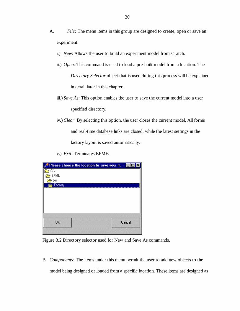
A. File: The menu items in this group are designed to create, open or save an
experiment.
i.) New: Allows the user to build an experiment model from scratch.
ii.) Open: This command is used to load a pre-built model from a location. The
Directory Selector object that is used during this process will be explained
in detail later in this chapter.
iii.) Save As: This option enables the user to save the current model into a user
specified directory.
iv.) Clear: By selecting this option, the user closes the current model. All forms
and real-time database links are closed, while the latest settings in the
factory layout is saved automatically.
v.) Exit: Terminates EFMF.
Figure 3.2 Directory selector used for New and Save As commands.
B. Components: The items under this menu permit the user to add new objects to the
model being designed or loaded from a specific location. These items are designed as

21
an alternative to the tool bar. The five menu items that represent the five different
experiment objects are listed below:
i.) Machine: By clicking on this menu item and experiment layout area
consecutively, the user can drop a new machine to the experiment layout. The
user can add a maximum of thirty four machines into the factory layout.
ii.) Transporter: By clicking on this menu item and factory layout area
consecutively, the user can add the transporter object to the factory layout.
Each modeled factory can have at most one transporter object, within this
single object different kinds of transporter units can be specified.
iii.) Repair: By clicking on this menu item and factory layout area consecutively,
the user can add the repair object to the experiment layout. Similar to the
transport object, each modeled factory can have at most one repair object.
Within the object the user can define the number of repairmen for the
experiment.
iv.) Inventory: By clicking on this menu item and the factory layout area
consecutively, the user can add the inventory object to the factory layout. Once
again, a given model will have at most one inventory object.
v.) Finished Goods: By clicking on this menu item and the factory layout area
consecutively, the user can add the finished goods object to the factory layout.
Just like Inventory object, a given model will at most have one Finished Goods
object.
C. Global: This menu option controls global commands, events and parameters such as
interest rate for cost calculations.

22
i.) Start: Starts the experiment.
ii.) Stop: Stops the experiment.
iii.) Report: Pulls up the reports window, which gives the statistical information
about the status of the model anytime through the experiment. Detailed
explanation about reports object will be given later.
iv.) Preferences: Shows the Preferences window, which is used for modifying
global parameters. Detailed information about the Preferences object will be
introduced later in this chapter.
v.) Initialize Statistics: This command is useful for initializing the statistics for all
the objects of the experiment. In experiments of stochastic nature, the statistics
that are collected in the transient period (i.e. the period before the system
reaches steady state) may have a bias. In order to “calm down” the output, the
user may trim this bias from the statistics. This command comes real handy in
such situations.
D. Options: All of the menu items but the last one under this group are utilized for
making Boolean decisions about the experiment.
i.) Bypass Transporter: This option is selected by checking on the appropriate
menu item. The option is used whenever the Transportation object is not used
in the experiment. Therefore all the batch transfers between objects happen
instantaneously. When the transportation object is added into the model, this
option is disabled.
ii.) Bypass Dispatcher: At the initialization of EFMF, this option is checked until
the dispatcher object is added to the layout. The option is used whenever the

23
model utilizes Kanban or CONWIP production system. Otherwise, the model
will not work due to the fact that there will be no raw material dispatch into
the system, hence no production.
iii.) Bypass Products Inventory: When the EFMF is started, this option is checked
until the Finished Goods object is added into the experiment. Without a
finished goods object, the experiment will work, but finished goods tracking
will be impossible.
iv.) Bypass Repair Shop: When the EFMF is started, this option is checked until
the Repair object is added into the experiment. The experiment will work
without this object; but even if a breakdown rate is specified for each machine,
there will be no breakdown, hence no repair.
v.) Routed: There are three possible path combinations for the batches that may go
through in an experiment. This and the following two options represent these
combinations. In the routed option, the batches go to the next machine as
specified in the parameter table’s Next Machine field.
vi.) Global: This option is quite useful at situations where there is more than one
machine in the production line to do the same job. By selecting this option, the
batch can go to any of the machines capable of processing that batch. The
machine that can process the next batch is specified in the Next Machine Type
field of the parameter table of the machine. The priority is given to the machine
that has the least number of batches in its input queue.

24
vii.) Sequential: If this option is selected, the batch will be routed sequentially
through the production line, i.e. the batch will go to machine one, machine
two, machine three and so on.
viii.) Stop Condition: One of the important aspects of GUIs is user interaction.
Clicking this menu item will pull up a window that is designed for establishing
a stopping condition for the emulation at a parameter-dependent instant. There
are three different options to stop an experiment:
• Stop push-pull when # produced: If a Kanban or CONWIP production
system is emulated, the machines will not demand any more batches if a
certain machine produces a certain number of products. The user defines
these two parameters.
• Stop factory when # produced: The experiment will stop when user-specified
machine processes a desired number of batches.
• Stop factory when duration completed: The experiment will stop after a user-
specified emulation period.
Figure 3.3 User interface of Stop Condition: (a) for the first two options and (b) for thelast option.
25
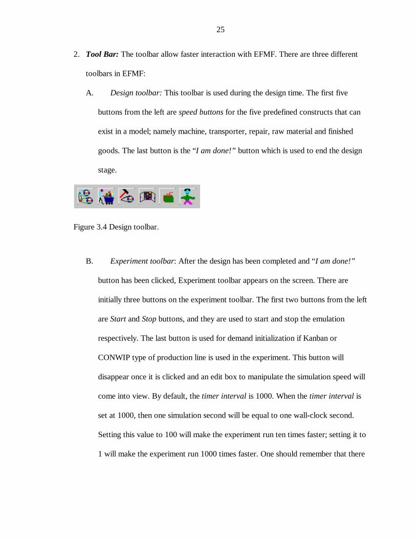
2. Tool Bar: The toolbar allow faster interaction with EFMF. There are three different
toolbars in EFMF:
A. Design toolbar: This toolbar is used during the design time. The first five
buttons from the left are speed buttons for the five predefined constructs that can
exist in a model; namely machine, transporter, repair, raw material and finished
goods. The last button is the “I am done!” button which is used to end the design
stage.
Figure 3.4 Design toolbar.
B. Experiment toolbar: After the design has been completed and “I am done!”
button has been clicked, Experiment toolbar appears on the screen. There are
initially three buttons on the experiment toolbar. The first two buttons from the left
are Start and Stop buttons, and they are used to start and stop the emulation
respectively. The last button is used for demand initialization if Kanban or
CONWIP type of production line is used in the experiment. This button will
disappear once it is clicked and an edit box to manipulate the simulation speed will
come into view. By default, the timer interval is 1000. When the timer interval is
set at 1000, then one simulation second will be equal to one wall-clock second.
Setting this value to 100 will make the experiment run ten times faster; setting it to
1 will make the experiment run 1000 times faster. One should remember that there

26
is a physical limitation on the speed of the experiment, which depends on the
hardware and operating system that EFMF resides on.
Figure 3.5 Experiment toolbar (a) before and (b) after initialization of the Kanban andCONWIP.
C. Termination toolbar (Phased out): The termination toolbar, as shown in Figure 3.6
was used in earlier versions of the software to save or clear the experiment prior to
exiting the program. In this version, the clear function is incorporated as a menu item
under File menu; and the settings and parameters are automatically saved once the
user exits EFMF.
Figure 3.6 Termination toolbar.
3. The Radio Group: As shown in Figure 3.7, this component allows the user to browse
through six states of EFMF. Explanations about these states are as follows:
Figure 3.7 Possible states.
A. Layout Adjustment: At this state, the user can drag and drop objects from the
toolbar to the layout area to design the model.

27
B. Edit Databases: This option allows the user to edit parameter tables of any
machine in the current model. When the user double-clicks on the icon that
represents the machine, a user interface that has a real-database link appears on
the screen, which is illustrated in Figure 3.8.
Figure 3.8 The user interface to access the parameter table.
C. Emulation: This state is generally used whenever EFMF runs the experiment.
Double clicking on an icon will bring the window associated with the object to
the screen. If the object window is already displayed, then EFMF will hide the
window.
D. All Visible: All object windows are made visible.
E. Hide All: This option is preferred when the speed of the experiment is the
number one priority. In that state, all object windows are hidden, which causes
to free up some memory space and to bypass some functions such as
animations.

28
F. Connect Processors: This option enables the user to connect the icons in the
experiment layout by straight lines. Currently, this function is used for cosmetic
purposes. A possible design recommendation is that the distances between
objects will be directly proportional to the length of the lines that are
connecting them.
3.3 Machine and Assembly Object
Machine and Assembly Object is used to emulate machine and assembly
operations (Figure 3.9). This is the only object that has to exist in a model. Each time the
user adds another machine into the model, a new instance of the Machine Object is created
and added to the array called Processors that resides in the Setup object. The machine
object window can take five different colors depending on the production system and state
of the machine. These colors and what they represent are shown in Table 3.1.
Table 3.1: Color-codes for the machine object
Color CodeBlue Machine is processing a MRP batchGray Machine is in the design stageGreen Machine is processing a CONWIP batchRed Machine is processing a Kanban batchYellow Machine is brokenWhite Machine is idle

29
Figure 3.9 Machine object.
Each machine has six parameter tables and one binary file to store the parameter
information and status of the machine during the experiment. Detailed information about
the six tables can be found at Chapter 4, Databases. The binary data file keeps the dynamic
information about the machine such as posted messages, current status, animation video
file name, machine ID and machine number.
The machine window provides some statistical information and current status of
the machine it emulates via the edit boxes, text boxes, tree views and gauges. Those
components are the essential part of the machine object; therefore they need to be
explained:
1. Outline component: This component provides information about the incoming and
outgoing batches of the machine object in a visually appealing fashion. There are two
levels; where the node represents the outgoing batch and the leaf denotes the incoming
batch.

30
2. “Input queue” and “Output queue” list boxes: These two list boxes show the batches
waiting in the input queue to be processed or the batches in the output queue to be
transported to the next machine, respectively. Number of batches in each queue is
shown below with a label.
3. “Batch Being Processed” Edit Box: This edit box gives information about the batch
that is currently being processed on the machine.
4. Edit Boxes for process and machine time statistics: These four edit boxes give
information about mean time and standard deviation about the process and the
machine. The Mc. mean time is the average time of processing a batch on the machine,
while Pr. Mean time also includes the time spent in the input and output queues. In
other words, Average Process Time = Average Input Queue Time + Average Machine
Time + Average Output Queue Time. The standard deviations of these two measures
are given in St. Dev edit boxes next to each one, respectively.
5. “Number produced” edit boxes: These edit boxes show the number of batches
produced.
6. “Start Time” and “Current Time” Edit Boxes: Information about the experiment start
time and current time is displayed here.
7. “Time Left” Edit Box: Remaining processing or setup time (in seconds) of the batch
currently being processed is displayed in this edit box.
8. “Throughput” Edit Box: Throughput is defined as “number of units produced in unit
time”. In EFMF, throughput is measured as the number of batches produced at one
simulation minute.

31
9. “Failure Rate” Edit Box: It shows the probability of machine breakdown at the next
simulation second. If the Bypass Repair option is checked, the value in the edit box
does not affect the operation of the machine.
10. “Status” Edit Box: Shows the current status of the machine and will display one of the
following messages:
• Blocked: This message appears when the output buffer is full and the machine
can not unload the finished product.
• Breakdown: This message appears when the machine is not working due to a
breakdown or maintenance.
• Idle: This message appears when the machine is not busy.
• Running: This message appears when the machine is processing a batch.
• Setup: This message appears when the machine setup is performed at the
moment. Note that setup times are different from the batch processing times. A
more illustrative explanation on setups can be found on Chapter 4, Databases.
11. Step Gauges Component: The machine object employs two step gauges. As shown in
Figure 3.9, the step gauges display the percent of the batch that is yet to be processed
and the percentage that has already been processed. Note that the two percentages do
not necessarily add up to 100%. The remaining portion represents the unit that is
currently being processed.
12. “Edit Dbase” Button: Opens a pull down database interface in the machine object for
parameter table, which enables the user to change some of the parameters associated
with a batch on the fly.

32
13. “Initialize Statistics” Button: Pressing this button will initialize statistics. While doing
experiments involving stochastic events, one might want to get rid of the effects of
transient period events. This option proves useful as it gets rid of the statistical bias
described above.
14. “Arrival” Button : Used for manual dispatches. This function is laying part of the
groundwork for the next phase of the software, where a supervisor object will be able
to do manual dispatching on factory being run on an another computer. This
functionality will be advantageous in situations at which the EFMF user will be
expected to respond to the unexpected changes in the current system. This option will
provide a great hand-on experience and facilitate Just-in-Time learning by creating a
real factory setting, where unexpected events always take place.
15. “K” Button : This button was used to initialize demands if Kanban or CONWIP
production system is used in the earlier versions of the EFML. It is not used in the
current version.
16. “Batch Size” button: This button is used to change the size of the outgoing batch. If
the incoming batch is selected at the product tree, the ratio of incoming batch to
outgoing batch is changed.
17. DBImage Box for Animation: This box plays the windows media file when the
animation option is enabled. Currently there are four different video files in the video
library.
The machine window also has two menu items under Options menu, which are
used to activate two functions depending on the user’s confirmation:

33
1. Keep log: By selecting this option, the machine keeps the historical information of
every batch that has been processed.
2. Animation: When this option is selected, video captures of various machining
operations are displayed on the image box of the machine window with stereo sound
to provide the virtual reality effects.
3.4 Machine Wizard Objects
In the earlier versions of the EFMF, the user modified the parameter tables by
using Database Desktop, which is a database utility program that can access Paradox
tables. In time many other simulation packages such as ARENA had completed their
migration from text-based and code-dependent user interfaces to a more user friendly
GUIs that would minimize the coding and correspondingly the design time. A need for a
more flexible user interface that would generate and modify the tables depending on the
needs of the experiment was evident. Parallel to that purpose, efforts were concentrated
on creating a set of GUIs that would create and edit all of the EFMF’s tables on-the-fly.
The first two of these GUIs are called Machine Wizard Objects and they are written
exclusively for the machine object (see Figure 3.10 and 3.11). For practical purposes,
these objects will be called Machine Wizard 1 and Machine Wizard 2.

34
Figure 3.10 Machine Wizard 1.
Figure 3.11 Machine Wizard 2.

35
Machine Wizard 1: As Figure 3.10 shows, Machine Wizard 1 object consists of a
Tree View component and four buttons and gives an overview information of the batch
processing structure of the machine. In order to increase user interactivity, a Tree View
component is used to show the product explosion. Tree View is the new version of the
Outline component that has been used in the machine object and it is one of the Windows
95 foundation classes. Descriptions about the four command buttons are as follows:
1. Add Outgoing Batch: When this button is pressed, Machine Wizard 2 is called to
add an outgoing batch into the list of outgoing batches associated with this
machine.
2. Add Incoming Batch: This button is used in order to relate an incoming batch to
one of the outgoing batches. Clicking on an outgoing batch and this button
consequently will do the job.
3. Delete: This button deletes one of the outgoing batches with its dependencies (i.e.
incoming batches) and their associated records from the parameter table.
4. Done: Closes the window and returns to the setup object. Also it launches the
procedures that prepare the setup file for the current machine.
Machine Wizard 2: This object is always launched with the command buttons in Machine
Wizard 1. In order to speed the parameter selection process, this window is decorated
with nine edit boxes and three radio groups (see Table 3.2).

36
Table 3.2 Types of edit boxes in Machine Wizard 2
Edit Box Name Description“Batch Name” Accepts a batch name.“Batch Size” Accepts the batch size.“Next Machine” If routed option is selected, this field accepts the next operation
of the batch.“Next Machine Type” If the global option is selected, this parameter accepts the next
machine type the batch will go. “# of Kanban” Accepts the number of Kanban cards this machine will use.“Unit Cost” Accepts unit cost of holding one unit at the inventory.“Mean” and “StandardDeviation” Edit Boxes
These four edit boxes are used for determining the first andsecond parameters of the distribution types used.
There are three radio group components in Machine Wizard 2. The first one
determines the production system (Kanban, MRP etc.) that is used to route the batch in
the production process and the latter two are used to determine the setup and the
processing time distribution types. Currently, four options are available in EFMF for time
distribution. They are exponential distribution, normal distribution, uniform distribution
and constant types.
3.5 Dispatch Object
The Dispatch object controls the raw materials inventory, dispatching of materials
into the system and detailed information about the product tree (see Figure 3.12). Raw
material tracking is handled through the two database grid components that allow the user
to interact with the raw material and order tables directly. In other words, the user can
change raw material inventory parameters such as number in inventory, maximum storage

37
capacity, and yellow and red alarm levels1. This kind of flexibility permits the user to
make on-the-fly decisions. Raw material ordering is achieved through two routines. In the
first routine, current inventory level is checked against auto order level. In a case when the
inventory level drops below the auto order level, new raw material is ordered according to
the order parameters that are specified by the user. In the second routine, the user
manually double clicks on the record that represents the raw material that he wishes to
order, and again, the order is placed according to the pre-specified parameters.
EFMF has the flexibility of performing two types of dispatches into the system,
namely periodic and manual. The periodic dispatch is done in every user-specified period
of time; and therefore it is deterministic. Once the user specifies the batch size and release
period for a specific batch and presses the PERIODIC button, the periodic batch
information is listed on the periodic dispatch list box that is located on the top right
corner of the window. Furthermore, the periodic dispatch remains in effect until the user
deletes it from the list with a double mouse click. For the manual dispatch, the user fills
in the manual release date and batch size by filling the appropriate edit boxes and clicks on
the MANUAL button. The user can change the periodic release parameters, which in turn
makes him capable of testing different release scenarios throughout the experiment.
Finally, the outline component on the top left portion of the window represents the
product explosion and it is a useful visual tool to see the entire product explosion.
The batch transportation from the raw material object to machines and between the
machines is done by the transporter object. If the user selects the bypass transporter
1 Detailed information about this parameter table for materials inventory (material.db) can be found atChapter 4, Databases.

38
option, the batches are immediately carried to the next station resulting a transportation
time of zero for each batch. On the bottom right portion of the window, the list box
displays the batches that are waiting in the output queue to be transported.
In the earlier versions of the software, this object had some problems with its user
interactivity in terms of building the product explosion tree and updating the raw material
tables. Since every new node on the product explosion meant a new product, related
tables from the finished goods object needed to be updated as well. Also, the times when
the finished goods object was not incorporated into the factory layout had to be accounted
for. In order to accomplish this industrious task, an attentive coding technique had to be
followed. As a result, three command buttons were selected to be the user interface to
process the tables for product explosion and the table product.db under finished goods
object database. Moreover, an object is designed to parse the user input and modify the
table product.db under raw material object database. This object is appropriately called
Product Tree Constructor (see Figure 3.13a and 3.13b).
As can be seen from Figure 3.13a and Figure 3.13b, the Product Tree Constructor
window takes two different forms depending on the type of product tree element that is
being added into the model. Adding a new product needs more parameters compared to
other options, since some of the parameters are used to refresh the finished goods tables.
An observant reader will soon realize that the four fields do not correspond to all the fields
in the finished goods table, due to the fact that some of the fields in that table are not yet
incorporated into the functionality of EFMF. However, the flexible design of the form
makes it as easy as adding a new edit box and writing a few lines of code to include the
new fields of the table, products.db.

39
While adding a new sub-component or a raw material, i.e. leaf, the edit box
“Machine number that will process this batch” is not used for a product. EFMF
automatically assumes that this number is 35, which is the ID of the finished goods object.
Figure 3.12 Dispatch Object.

40
Figure 3.13 The form Product Tree Constructor (a) when adding a new product and (b)when adding a new intermediate product or raw material (component).
3.6 Finished Goods Object
The Finished Goods object keeps track of the finished goods inventory as well as
the incoming sales orders (see Figure 3.14). By using two Database Grid components, the
Product object provides a user-friendly interface, which shows the inventory movements
and orders dynamically. The customer demand is created through a parameter-driven
process. Also the user can create a virtual random demand by double clicking on the
Products Stored Database Grid. Three kinds of orders are defined for our purposes:

41
Figure 3.14 Products object.
• Filled: The orders that were shipped on time.
• Late: The orders that were not shipped on time.
• Cancelled: The orders that are cancelled. Canceling an order in the Products object is
easy; double clicking on the Outstanding Orders Database Grid will do the job.
The Products Stored Database Grid is a component that lets the user to change
the system parameters dynamically. After finding the parameter that needs to be changed,
simply type the new value for this parameter and press enter.
In the future versions of the Products object the following functions are planned to
be incorporated into its nature:

42
1. User defined demand: With this functionality, the user will be able to define the
parameters of an order (number of units ordered, order cost, order canceling cost,
lead-time etc.). This will enable the user to react to the stochastic changes in the
system which in turn, facilitate the Just-in-Time learning.
2. Supply Chain Management: By using the add-in functionality of the TCP/IP
component of Borland Delphi 3.0, two or more factories will be able to “speak” with
each other therefore forming the individual links of the supply chain.
3.7 Transportation Object
This object is accountable for emulating the transportation of all units in the model
(Figure 3.15). Generic information about each transport unit is shown in the grid box of
the transportation window. Transportation object “listens” the commands from machine
and dispatch objects in order to execute the transportation between two processors. There
are three steps in using a transporter. First, the machine or the dispatch object requests a
transporter by sending a message to the object. Then the transporter object responds by
allocating one of the transporters found in the transporter list.
Consequently, the transporter picks up the batch, holds the batch for a specific
amount of transportation time, which is determined by the user-defined parameters, and
finally releases the batch to the destination station.
In the case of multiple transporters in the system, there are two issues regarding
their assignment to the batches. First, a machine may request a transporter and more than

43
one may be available. In that case, there are three different priority schemes to be followed
depending on the user’s selection:
1. First available: Activated by the “First Available” button. It selects the first available
unit that can transport the batch to the destination machine.
2. Fastest First: Activated by the “Fastest First” button. It selects the transporter that
can transport the batch the fastest.
3. Manual: Activated by the “Manual” button. By double clicking on the wait queue list
box, the user carries out the transportation requests manually.
Currently, the type of transporters EFMF uses can be regarded as Trail-Free
transporters. Trail-Free transporters can move freely through the system without creating
delays by reason of congestion in the system. Total transportation time for a batch
depends on the capacity, velocity and distance to be traveled.
Other than responding to the transportation messages coming from other machines
or dispatch unit, the Transportation object is independent from the rest of the simulation.

44
Figure 3.15 Transporter Object.
The transportation object embodies five tables, two of which contain parameter
information. In earlier versions of EFMF, the parameter file had to be created and
modified by using a database utility program at the user’s disposal. Although a user
interface was developed for adding a new transporter into the model, it was not
satisfactory in terms of user-friendliness and capability (see Figure 3.16). In order to solve
this problem two objects were developed and one existing object is modified to create and
edit the parameter tables as well as parse the user’s input:

45
Figure 3.16 New Transporter object (old version).
1. Distance Matrix: This user interface is developed in order to create and modify the
distance.db table, which the EFMF uses to calculate the total transportation time
(Figure 3.17). An item in the ith row and jth column represents the distance between
two objects where the departure object is i, and the destination object is j.
Figure 3.17 Distance Matrix

46
2. Transporter Design: Designed to create the file Trans.db, which holds the generic
information about each transporter and its maximum capacity to carry all the outgoing
batches in the simulation model, this object is part of the solution to the user-interface
problem of the Transporter object (see Figure 3.18). When the object first appears, it
immediately lists all the batch names in the Trans.db which represent all the batches
that can be transported from one processor to another in the simulation model. The
user can add or take away batches from the simulation model and the table is
appropriately updated as the user clicks ‘OK’ button.
Figure 3.18 Transporter Design
3. DBNavigator: As an earlier version EFML user will recall, this object originally
served as the real-time table-editing interface for machine objects. After a smart
modification, it was ready for the task of editing Trans.db, the table which shows the
generic information (speed, quantity and capacity) of each type of transporter unit

47
under Transportation object database. It is used to define the parameters and quantity
of each transportation unit.
The transporter object can also keep a log file of every transportation activity that
has taken place throughout the experiment. To activate the option, the user simply clicks
on the “Log File” check box.
In spite of having a robust design and user friendly interface, the transporter object
can be improved further. The following may have the focus areas in future versions of
EFMF:
Figure 3.19 DB Navigator object
1. Guided Transporters: As explained before in this section, EFMF uses Trail-Free
kind of transporters. However in real life, Guided Transporters have unique effects on
a plant layout because of their nature. These transporters are useful for simulating
Automated Guided Vehicle (AGV) systems or distribution center systems that employ
some kind of a moving cart on predefined path.

48
2. Additional capabilities on a schedule of a transporter: Currently, EFMF assumes
that a transporter always goes back to its initial location after it finishes the job of
transporting a batch. But alternative situations may occur, such as staying at the last
station visited, returning to a machine park, or following a looping pattern, which can
be predefined by the user.
3. Conveyors: Another type of transportation medium that is widely used in factory
settings is a conveyor. They are different from Trail-Free transporters in a sense that
they can move in a single direction with limited space.
3.8 Repair Object
The Repair object emulates all machine repairs within the model (Figure 3.20). The
object incorporates seven tables into its functionality. These tables contain the historical
data as well as the overall performance information about the individual repair objects.
The repair object must receive a repair message in order to execute a repair on the
target object. Immediately upon receipt of such message, the repair request is saved in a
queue and processed according to the first-come first-serve method. However, the user
may change the order of repairs by double clicking on an item in the list box in which the
repair requests are displayed. That will put the selected repair request on top of the wait
queue.
The progress bars provide visual aid to the user on the percent of the repair job
completed. Also, the user can find detailed information about a specific repair job on the

49
Repair Machines grid. All statistics about all repair activities are maintained in the Repair
database.
In the current version, the user can change the number of repairmen in the repair
object. This option allows the user to test the system performance against the number of
repair resources used.
The repair object is a product innovative thinking considering the fact that no other
major simulation software embodies such or a similar object in existence. Although quite
innovative, the object may benefit from further improvements. These improvements
include:
1. A more parameter-dependent repair process: Currently, the repair times are
randomly generated. Repair times can be batch-dependent and parameter driven. This
means adding a new data source to the environment, most probably a Paradox table
that will contain repair times with respect to each batch processed in the model. Also
other parameters such as lead-time for a repair or number of repairmen needed, can be
added to the functionality.
2. Priority rules: Unless the user changes the order of a repair, there is only one priority
rule for a repair, which is first-come first-serve. Many other repair allocation schemes
can be added such as
• Cyclic: Cycling through the repairmen. This option will level out the utilization of
each repairmen.
• Priority: Each machine can be assigned a priority number for a repair. A similar
field exists in the machine database for batch processing priority.

50
• Shortest repair time: The repair job is allocated according to the length of the
repair time. The shortest repair time job will get the highest priority.
• Longest repair time: The repair job is allocated according to the length of the
repair time. The longest repair time job will get the highest priority.
Figure 3.20 Repair object

51
CHAPTER 4 DATABASES
4.1 Introduction
The databases in the EFMF contain all the historical information as well as the
experiment parameters. These Paradox databases are created by using add-in
functionalities of Borland Database Engine and edited by Database NaviGator, which is
designed as part of this thesis. The structure and information about each database will be
discussed in detail in this chapter.
4.2 Machine Library
This database provides generic information about the types of machines used in the
virtual factory that is built. The database is appropriately called machine.db (Table 4.1)
and it is located in the directory “Database_Directory\factory”.
The user can add as many different machines as he wants. This will ensure that
each machine will specifically be tailored to the experiment being carried. Four example
machines are shown in Table 4.1 The explanation of each field on this database can be
seen below:
1. Machine Index: This field is the designated for the identification of the machine.
This field is keyed meaning that each machine has a unique index number.

52
2. Type: This field identifies the class this particular machine belongs to.
3. Explanation: Explanation, comments/suggestions about the machine is provided
here.
4. Value: Current dollar value of the machine is indicated here.
5. Failure Rate: Current failure rate of the machine is indicated here. This number
changes between zero and one and shows the likelihood of that machine to fail in
the next simulation second. A value of say, 0.35 indicates that the machine will
have a failure probability of 35% in the next simulation second.
6. Defective Rate: Defective percentage of products that the machine produces for
each batch.
7. Animation File Name: The audio-video (*.avi) file name of the machine is
described here. These files are located in the following directory:
“C:\efml\db\machine\avi\”.
8. Number of Man Required: Denotes the manpower required to operate the
machine.
9. Power Rating (kW.): Power consumption per unit time for each machine.
10. Width (cm.): Width of each machine. The unit is centimeters.
11. Breadth (cm.): Breadth of each machine. The unit is centimeters.
12. Height (cm.): Height of each machine. The unit is centimeters.
13. Weight (kg.): Weight of each machine.
14. Spindle Speed (rpm): Engine rotation speed for each machine in terms of
revolutions per minute.

53
Table 4.1: Machine Library, machine.db.
Machine Index 1 2 3 4
Type CA CR DS FAExplanation Controller
AssemblyCarafeAssembly
DeburringStation
FinalAssembly
Value 3000 250 2200 550Failure Rate 0.005 0.003 0.002 0.008Defective Rate 0 0 0 0.10Animation FileName
Finishing Lasercut Milling1 Turn
Number of ManRequired
1 2 1 3
Power Rating(kW.)
12 4 17 35
Width 200 300 200 200Breadth 3700 2300 5500 2100Height 5000 2700 2100 3321Weight 1000 12500 9600 500Spindle Speeds 3000 3000 3000 3000
4.3 Factory Setup Object Database
The experiment setup database, factory.db (Table 4.2) is located in the directory
“Database_Directory\factory”. The description of each field is shown below:
1. Machine ID: This is a keyed field, which ensures that each machine has a unique
ID. The messages sent to this machine, the databases, icon and the form used by
that machine use this distinct ID to separate the machine from other objects.
2. Machine #: This field is used to sort the machine in the machine library.
3. Computer #: Marks the specific computer that the machine will become active.
4. Input Buffer Size: Maximum queue length for the incoming batches.
5. Output Buffer Size: Maximum queue length for the outgoing batches.

54
6. X-Position: X-coordinate of the machine icon in the screen. The top left corner has
the coordinate of (0, 0).
7. Y-Position: Y-coordinate of the machine icon in the screen. The top left corner has
the coordinate of (0, 0).
8. Active: Indicates the status of the specific machine on a specific computer. 1 means
the machine is active, 0 means the machine is not active.
Machine and factory setup objects all possess binary data files that contain dynamic-state-
information. In other words, those binary files provide the current configuration or a
snapshot of these objects. Should the program be terminated or EFMF crashes for an
unknown reason, these binary files make it possible to recover the instance just before the
termination. These files have the extension of “*.dat” and because of their dynamic nature,
they are appropriately located in the location “Database_Directory\machine\dynamic”.
Table 4.2: Machine library (factory.db) example.
MachineID
Machine#
Computer#
InputBufferSize
OutputBufferSize
X-Position Y-Position Active
1 2 1 15 15 10 10 12 3 1 15 15 10 20 13 6 1 10 10 10 30 14 5 1 10 10 10 40 15 1 1 50 50 10 50 16 4 1 25 25 10 60 1
4.4 Machine and Assembly Object Database
The Machine and Assembly Object has six dedicated database tables. These six
tables end with the Machine ID that are defined in Machine Library, factory.db. The first

55
two tables contain the experiment parameters, while the remaining four hold the machine
information during the experiment. These files are empty at the beginning; hence they are
located at “Database_Directory\factory\machine\empties”. Here are the four tables:
1. Batchi[Machine ID].db: Holds information about the batch in progress (Table
4.3).
2. Iqueue[Machine ID].db: Holds information about the input queue (Table 4.3).
3. Oqueue[Machine ID].db: Holds information about the batches in the output queue
(Table 4.3).
4. Hist[Machine ID].db: Keeps date and time stamped information of events
occurred in the machine. Usage of this table is optional to the user.
The first three database tables that contain input queue, output queue and batch in
process information are identical in structure and have the following fields:
1. Batch: Name of the batch.
2. Batch Size: Number of parts in the batch.
3. Bad #: Number of defective parts in the batch.
4. Batch No: Number identifier of the batch.
5. Date In: Batch receiving date.
6. Time In: Batch receiving time.
7. Kanban: Production system used.
8. Cost: Present cost of the batch.
9. CONWIP Start: The first machine in the CONWIP line. This is used if the current
machine is the first in the CONWIP line.
10. SetupTime Mean: Average setup time of the batch.

56
11. Time Mean: Average processing time of the batch.
12. DueDate: Batch due date.
13. DueTime: Batch due time.
As soon as a machine receives a batch, the related data is appended to its input
queue table. As the batches are processed, the related record moves upward in the input
queue file. When the time comes to process the batch, it is transferred to the work-in-
progress. The work-in-progress table can contain at most one record, due to the fact that
a machine can and will process one batch at a time. After the entire batch is processed the
record is finally transferred to the outqueue table, where it waits to be transported to the
next processor in the production line.
The fourth table in the “Database_Directory\factory\machine\empties” directory is
the history table which has the filename structure of hist[Machine ID].db. It has the
following fields:
1. Event Type: Stores the type of event documented. There are four kinds of events:
1: Batch Arrival
2: Batch Departure
3: Machine Breakdown
4: Machine Repair
Although in the current system there are four kinds of events, it is always possible
to define more events.
2. Time: Event time.
3. Date: Event date.
4. Batch name: Name of the batch sent or received.

57
5. Batch size: Size of the batch sent or received.
6. Kanban cards: Number of Kanban cards.
7. Trigger: Trigger level of Kanban cards. A machine requests batches from the
upstream station only after the number of free cards equal to the trigger level.
8. Demands: Number of Kanban Demands when the event happened.
The two tables that contain the parameter information are called batch and setup
tables, and appropriately they have the filename formats of batch[Machine ID].db and
setup[Machine ID].db, respectively. The former file contains the batch information while
the latter is tailored for setup only. They are kept at the location
“Database_Directory\factory\machine\”.
The square matrix form of the setup database makes it possible to emulate
sequence dependent setups and clearly saves considerable amount of design time when
compared to the other simulation packages such as ARENA. The transition is from the
column batch to the row batch. An example setup table is given in Table 4.3. The cells are
in the format of [Parameter Distribution Type]/[First Parameter]/[Second Parameter].
Table 4.3: An example Setup table for a machine.
Batch 1 Batch 2 Batch 3Batch 1 C/3/3 C/4/4 C/5/5Batch 2 U/2/5 U/0/5 E/6/6Batch 3 N/7/3 N/3/1 N/9/3
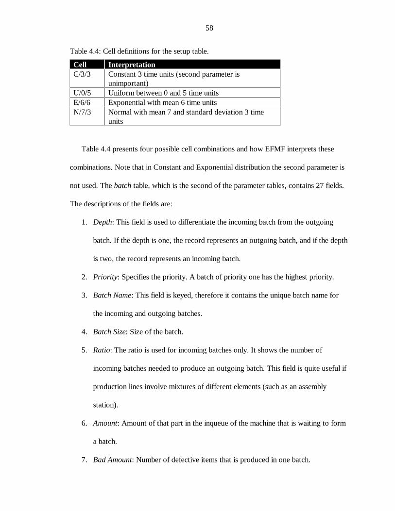
58
Table 4.4: Cell definitions for the setup table.
Cell InterpretationC/3/3 Constant 3 time units (second parameter is
unimportant)U/0/5 Uniform between 0 and 5 time unitsE/6/6 Exponential with mean 6 time unitsN/7/3 Normal with mean 7 and standard deviation 3 time
units
Table 4.4 presents four possible cell combinations and how EFMF interprets these
combinations. Note that in Constant and Exponential distribution the second parameter is
not used. The batch table, which is the second of the parameter tables, contains 27 fields.
The descriptions of the fields are:
1. Depth: This field is used to differentiate the incoming batch from the outgoing
batch. If the depth is one, the record represents an outgoing batch, and if the depth
is two, the record represents an incoming batch.
2. Priority: Specifies the priority. A batch of priority one has the highest priority.
3. Batch Name: This field is keyed, therefore it contains the unique batch name for
the incoming and outgoing batches.
4. Batch Size: Size of the batch.
5. Ratio: The ratio is used for incoming batches only. It shows the number of
incoming batches needed to produce an outgoing batch. This field is quite useful if
production lines involve mixtures of different elements (such as an assembly
station).
6. Amount: Amount of that part in the inqueue of the machine that is waiting to form
a batch.
7. Bad Amount: Number of defective items that is produced in one batch.

59
8. Next Machine: The following two fields are essential as they are used to specify
the next machine that the outgoing batch will go to. This field specifically
designates the machine by using its machine number. The experiment has to be in
routed mode.
9. Next Machine Type: The next machine is stipulated by sending the outgoing batch
to the first available machine in the desired machine group.
10. Cost: Production cost of the batch for that machine only.
11. Duedate: The date is used as a priority measure in a case where the earliest due
date priority rule is used to determine the batch processing order.
12. Pr. Time Dist. Type: This field determines the distribution type that will be used
for the processing time. Currently there are four kinds of distributions:
C: Constant processing time. Only the First Parameter field is used, which
determines the constant processing time.
E: Stands for Exponential distribution. Again only the First Parameter field is used
for the mean.
N: Denotes Normal distribution. It uses the First Parameter field as the mean and
Second Parameter field as the standard deviation.
U: Stands for Uniform distribution. First Parameter field defines the lower
boundary while the Second Parameter field defines the upper boundary.
13. First Parameter: The usage of this field is discussed in detail in Pr. Time Dist.
Type.
14. Second Parameter: The usage of this field is discussed in detail in Pr. Time Dist.
Type.

60
15. Batch No: This field keeps the batch id, which is unique for every batch.
16. L/M Ratio: Represents labor to machine ratio, which is the number of operators
needed to process the batch.
17. L/C Ratio: Stands for labor to cost ratio, unit cost of labor to process the batch.
18. Tree Level: It is used to determine the level of the batch on the product explosion
tree on the dispatch object.
19. No. Parts/Cycle: This field is used to simulate experiments where one cycle of
production produces more than one parts per cycle.
20. Acceleration Rate: This field shows the number of “real clock seconds” that one
“emulation second” correspond to. This field is one by default. Note that,
increasing the value on this field will greatly degrade accuracy. In later versions of
the software, this field is not used.
21. # of Kanban: Number of Kanban cards for this batch. This field is used for
outgoing batches only.
22. Level: Level of the Kanban card.
23. Trigger Level: Determines the level where the machine requests the incoming
batches from the preceding station.
24. Kanban Out: Designates the production system this machine obeys. Table 4.5
explains each of the possible values this field can get. Because of the devised
graphical user interface, this field is not directly accessible by the user.
25. Left Over: Used to trail surplus of the incoming parts if odd batch sizes are used.

61
26. Total Inventory Cost: Cumulative inventory cost is stored here. This field is
updated at 12:00 AM in every experiment day by using the appropriate
parameters.
Table 4.5: The definition for the Kanban Out field of the batch table.
Symbol Description Card NumberK Kanban batch User specifiedN Non-Kanban batch (MRP batch) -1NK Current machine non-Kanban, following machine
represents a Kanban line-1
SW First machine of a CONWIP line User specifiedW Intermediate machine of a CONWIP line -1EW Last machine of a CONWIP line. Following machine
represents a MRP line.-1
WK Last machine of a CONWIP line. Following machinerepresents a new CONWIP or Kanban line.
-1
KN Current batch is a Kanban batch and following machinerepresents a non-Kanban line.
User specified
NN Batch does not follow Kanban rules. -1
4.5 Transportation Object Database
The object is used to simulate any kind of transportation a batch can possibly go
through. The transportation databases are stored in “Database_Directory\factory\trans\”.
This directory contains six tables, four of which are empty initially and updated
dynamically during the emulation. Explanation about the four dynamic tables are given
below:
1. Waiting.db: Contains the list of batches that are waiting for the release messages
to be transported.
2. Log.db: This is the log file that keeps track of every transportation happened in the
experiment. It has the following fields:

62
• Batch: Name of the transported batch.
• Transporter: The transporter id.
• From: Identifier of the processor that the batch leaves.
• To: Identifier of the processor that the batch goes to.
• Arrival: Batch arrival time.
• Start: Transportation start time.
• Finish: Transportation finish time.
3. Queue.db: This table stores information about the batches that are waiting in the
input queue to be transferred.
4. Backup.db: Keeps are backup of the transports that are carried out in the
experiment.
The remaining two tables store the parameter information for the Transportation
object. Their explanations are as follows:
1. Trans.db: This table stores the information about each kind of transporter that is
used in the experiment. The associated file with this table is dynamically created
during the design time. The file contains the name of the transporter, its speed, its
quantity and finally its capacity for each batch. An example trans.db can be seen in
Table 4.6.
Table 4.6: Trans.db example.
Transporter Speed Quantity Wheel Door ChairForklift 10 2 40 50 50Trolley 20 5 25 10 20

63
2. Distances.db: Stores distances between all the objects in the experiment and
created dynamically during design time. It is not accessible during the run-time.
The numbers in the column and row headings represent the windows ID of the
objects. According to this convention, numbers 1 through 34 denote machine
numbers, while 301 denotes Dispatch, 302 denotes Transporter and 35 denotes
Finished Goods objects. An example configuration is presented in Table 4.7.
Table 4.7: A distances.db example.
Machine 1 2 35 301 3021 0 1 5 63 32 1 0 22 5 235 5 22 0 25 54301 63 5 25 0 44302 3 2 54 44 0
4.6 Finished Goods and Shipment Object Database
This object uses five tables. The files are located at
“Database_Directory\factory\products”. This object is used to track the finished goods
movement. In the current system, it serves as a counter for all the entities that leave the
modeled system. Furthermore, virtual demand tracking can be performed on this object as
well. The detailed descriptions of these five tables are as follows:
1. Inset.db: This table is used to trace the generic information about placed orders,
such as number, last order ID etc., and used as an initialization table. Detailed
information about the fields can be seen at Table 4.8.
2. Orders.db: It keeps a detailed information about every placed order and contains
statistics about the order satisfaction. For details, see Table 4.9.

64
3. Osorders.db: This table keeps track of the number orders that have not yet
reached their due date. For details, see Table 4.9.
4. Outqueue.db: This table serves to record the finished goods that have not yet
shipped. Check Table 4.10 for the detailed explanation of the fields.
Table 4.8: Structure of Inset.db
Field DefinitionTime Initial TimeDay Initial DayOrderID Last Order IDBnumber Last Batch Number
Table 4.9: Structure of Orders.db and Osorders.db.
Field DefinitionOrder ID Order identification numberMaterial Name The name of the raw material that has been orderedSupplier Name Name of the supplier that the raw material has been orderedOrder Release Date The date at which order is releasedExpected Date The date at which order is expectedJIT(YES/NO) Boolean field to determine if Just-In-Time manufacturing system
is utilized.# Units Ordered Number of units orderedOrder Status Outstanding, Delivered or CanceledTotal Order Cost Cost of the total order in dollarsUnit Cost Unit cost of material of the orderOrder Canceling Cost Order canceling penalty in dollarsLast Date to Cancel Last date to cancel the orderReal Arrival Date The date at when the order is receivedDefective Percentage Percentage of imperfections in the received batch
Table 4.10: Outqueue.db
Field DefinitionBatch The name of the batch that is waiting to be transportedSize The size of the batch that is waiting to be transportedBad Amount The number of defects in the batchNext Machine The ID of the next machine that batch will goNext Machine Type The type of the next machine that batch will goCost Current cumulative cost of the batch

65
Due Date The due date of the batchBatch No Number of the batchMessage Related transportation message of the batchTime Leaving time
5. Product.db: This table keeps the experiment parameters for the Finished Goods
object. The table Product.db has the following fields:
(1) Product name: The name of the finished good in the experiment.
(2) # in Inv: The number in the finished goods inventory.
(3) Max Storage Capacity: Maximum capacity of the storage area for the
finished good that is specified in Product name.
(4) # Outstanding Orders: The number of orders that are not yet reached to
their due date.
(5) Manufacturing Policy: This field is not currently in use, but it is designed
to reflect the changes in the manufacturing scheduling policy.
(6) # Total Orders Placed: Total number of orders taken for the finished good.
(7) # Total Orders Shipped: The number of orders that has been shipped to the
customer.
(8) # Total Orders Canceled: This field is used to track the number of orders
that are cancelled by the operator or the supervisor object. The two mentioned
objects existed in earlier versions of the software and they are not currently in
existence. Hence, this field is not used, but restored for compatibility.
(9) # Total Orders Shipped: The number of units of the finished good that was
shipped.

66
(10) Yellow Alarm Level: This field is used to warn the user that the inventory
level is getting low. It will be crucial in the future design of the Finished Goods
and Shipment Object when the inventory level will be shown in colors to improve
user interactivity.
(11) Red Alarm Level: It is used to pinpoint the critical inventory level where
intervention is necessary.
(12) Auto Production Level: This field represents the level at which raw
materials will automatically be made available for production.
(13) # Bad Units: Represents the number of finished goods that are defective or
does not reach the predetermined quality standards.
(14) # Bad Units Found: Stands for the number of bad units. The Quality
Control (QC) object in the earlier versions of the software used this field. As the
QC object was abolished, this field is not used anymore. It is kept to preserve
compatibility.
(15) # Units Controlled: This field was used by the QC object to report about
the quality control tests being performed used this field. It is not used in the
current version and kept to preserve compatibility.
(16) # Bad Units Mistaken: Represents the number of defective goods that have
been accepted as a result of the β (Type II) error. In plain English, number of bad
units that have passed the quality test.
(17) # Good Units Mistaken: Represents the number of good units that have
been rejected as a result of the α (Type I) error. Namely, number of non-defective
units that have failed the quality test.

67
(18) # Scrapped: Number of units scrapped during production process.
(19) # Returned: Number of products that are returned from the customer as a
result of some form of customer dissatisfaction.
(20) Total lead-time: Total product lead-time.
(21) Average lead-time: Total lead-time divided by number of filled orders.
(22) Unit Volume: Unit volume of each type of finished goods.
(23) Unit Weight: Weight of each unit of finished good.
(24) Volume Allocated: Total space allocated to this particular product in the
storage area of the facility.
(25) Volume Used: Current space usage for the product.
(26) Average Unit Cost: Average cost to produce one unit of the product.
(27) Total Inventory Cost: Total inventory cost of this finished good.
(28) Total Canceling Cost: Total cost for the orders that have been canceled.
(29) Total Transportation Cost: The costs that have been incurred from the
transportation of finished goods to clients.
(30) Total QC Cost: This field represented the total quality control costs. After
abolishing the Quality Control object, this field ceased to be of any use,
nevertheless it is kept to preserve compatibility.
(31) Total Holding Cost: Total cost of holding inventory in the warehouse.
(32) Total Loading Cost: Total cost of loading finished goods to the
transporters such as plane, truck or ship etc., in order to ship them to clients.
(33) Dimension 1: The width of the one unit of shipment box.
(34) Dimension 2: The height of the one unit of shipment box.

68
(35) Dimension 3: The depth of the one unit of shipment box.
(36) Image File Name (Good): This field was used during the manual quality
control process and it represented the “good” form of the product. After the
elimination of the quality control object, it is kept to only preserve compatibility.
(37) Image File Name (Bad): This field was used to identify the image file name
that would represent the “bad” form of the product. It shares the same destiny with
the previous field.
(38) Automatic Order Quantity: This field is used in specifying the automatic
order quantity.
(39) Automatic Order Interval: This is used to determine the duration between
automatic orders.
(40) Automatic DDate Interval: This field is designated for the interval from the
order date to the shipping date.
(41) Last Request Date: The date of the last request for the finished good.
(42) Setup Time: This field denotes the time to process a shipment.
(43) Gauge Image: The file name of the image that is used for the gauge level to
show the current inventory.
(44) # of Kanban: Represents the maximum number of Kanban cards that can
be used. Applicable to Kanban lines only.
(45) Demanded: Number of Kanban cards that have been demanded from the
system.
(46) Kanban Out: This field defines the type of production system the
experiment uses.

69
4.7 Dispatch Object Database
The Dispatch object has seven tables. Five of these tables are empty at the start of
the emulation and change dynamically throughout the experiment. The remaining two
contain the parameter information. They are located in
“Database_Directory\factory\dispatch”. The four tables that record the intermediate
experiment information are:
1. Inset.db: This table contains the order number and information about the current
time and day. It has the exact same structure as the Inset.db file of the Finished
Goods and Shipment object (see Table 4.8).
2. Orders.db: Holds information about the raw material orders during the emulation
process. It has the exact same structure as the Orders.db table of the Finished
Goods and Shipment object (see Table 4.9).
3. Osorders.db: This is the table that records the outstanding orders; i.e. the orders
that have not been received yet. Again, it is the replica of the table Osorders.db of
the Finished Goods object (see Table 4.9).
4. Outqueue.db: This table is functions to record the batches that are waiting to be
transported. Once again, this table is identical to the one of the Finished Goods and
Shipment object (see Table 4.9).
5. Periodic.db: This table keeps the periodic dispatches in the system. It has one
field, namely Dispatches that keeps the formatted message of the Dispatch object.

70
The Dispatch object reads, parses and updates that message during the course of
the emulation.
• Product.db: This table contains the raw materials inventory information. Some fields
of this table change at the time of the experiment to reflect the inventory changes. The
fields are defined as below:
1. Depth: This field represents the depth of the item in the product tree. If the depth
is one, it is a final product, if it is two, the node should be processed in order to
constitute the final product. As one move away from the final product, this number
increases.
2. Batch: This field represents the name of the batch in the production process.
Again, it can stand for one of the following: Raw material, intermediate product or
a finished good.
3. Size: Stands for size of the batch. This field can be altered any time during the
emulation, allowing the user to change the parameters during run time.
4. Ratio: Represents the ratio of the incoming items to the outgoing item. If four
doors are used for one car assembly, the Ratio would be four.
5. Next_mch: Used to define the next machine that the outgoing batch is sent to.
6. Cost: Cost of the batch.
7. Next machine ID: ID number of the next machine.
8. Demanded: This is field is used if a Kanban production system is in effect and
stands for the number of Kanban batches that have been demanded.

71
9. Kanban Out: This field stands for the production system used. This field is used to
distinguish the Kanban type production from the others. The possible values this
field can assume are explained in Table 4.5.
10. Batch_ID: Stores the unique ID number for the batch.
11. PWeek: Represents the number of weeks between each periodic dispatch.
12. Pday: Represents the number of days between each periodic dispatch.
13. PHour: Represents the number of hours between each periodic dispatch.
14. PMinute: Represents the number of minutes between each periodic dispatch.
15. PSecond: Represents the number of seconds between each periodic dispatch. A
user may define a dispatch period by selecting any combination of 11-15.
• Material.db: This table stores the parameter information about the raw materials in the
system. Some fields of this table such as “# in Inv” change during emulation. This
table is one of few tables that the user can directly access and modify in the middle of
the experiment. The field definitions of this table are as follows:
1. Raw material: Represents the raw material name. This field is keyed and
therefore enabling each record in this table to be unique.
2. # in Inv: Designates the number of items that are currently in stock.
3. Max Storage Capacity: Indicates the maximum space allowed for this
particular item.
4. # Outstanding Orders: Represents the number of outstanding orders that have
been placed, but not yet received.

72
5. Ordering Policy: This field stands for the policy under which raw materials
inventory control will be carried on. For example, EOQ represents the Economic
Order Quantity Model.
6. # Total Orders Placed: The total number of orders placed for this material.
7. # Total Orders Arrived: Keeps the total number of orders received for this
material.
8. # Total Orders Cancelled: Records the number of cancellations of raw material
orders by the user.
9. # Total Units Arrived: This keeps the total number of raw material units
shipped to the factory.
10. Yellow Alarm Level: This field is used in conjunction with the inventory level
indicator and determines the background color of the database edit box that shows
the current inventory level. If the inventory level is lower than the value specified
in this field and higher than the value specified in Red Alarm Level field, the
associated database edit box turns yellow.
11. Red Alarm Level: This field informs the fact that the inventory is reaching to a
critical point, where intervention might be necessary. Just like the preceding field,
this field is used to determine the color of database edit box that shows the current
inventory level for the examined raw material. If the inventory level drops below
this value, the associated database edit box turns red.
12. Auto Order Level: This is the automatic order level at which the system places
an order for the associated raw material. Typically this number is less than the Red

73
Alarm Level, so that even if the user do not place orders, the system will. Setting
this field to a negative value will disable the automatic order option.
13. # Bad Units: Represents the total number of imperfect units. The value in this
field is based on the incoming product parameters.
14. # Bad Units Found: Represents the total number of imperfect units that the
user found. The Quality Control (QC) object in earlier versions of the software
used this field. Since the QC object no longer exists in the software, this field is not
used anymore. It is kept only to preserve compatibility.
15. # Units Controlled: Number of units that the QC object inspected, this field is
not used anymore. It is kept only to preserve compatibility.
16. # Bad Units Mistaken: Stands for the defective number of products that have
been accepted as a result of the β (Type II) error. In other words, number of bad
units that have passed the quality test, this field is not used anymore. It is kept only
to preserve compatibility.
17. # Good Units Mistaken: Stands for the defective number of products that have
been accepted as a result of the α (Type I) error. In other words, number of bad
units that have passed the quality test, this field is not used anymore. It is kept only
to preserve compatibility.
18. # Scrapped: Number of units that are rejected and dumped during the
production process, this field is not used anymore. It is kept only to preserve
compatibility.

74
19. # Rejected: Number of raw material units that are rejected due to the lack of
quality and sent back to the wholesaler, this field is not used anymore. It is kept
only to preserve compatibility.
20. Total lead-time: Sum of all the historical lead times for the raw material.
21. Average lead-time: This field is calculated by dividing Total lead-time by the
number of batches received.
22. Unit Volume: Represents the volume of each unit of raw material.
23. Unit Weight: Represents the weight of each unit of raw material.
24. Volume Allocated: Presents the maximum allowable storage space for the item
in question.
25. Volume Used: The actual volume used by the current level of the raw material
inventory.
26. Average Unit Cost: Displays the average cost of one unit of raw material since
the last initialization of statistics.
27. Total Inventory Cost: Exhibits all the costs associated with holding the raw
material in the inventory such as storage, control, total cost of acquiring the
material etc.
28. Total canceling Cost: Aggregate costs of cancelled orders.
29. Total Transportation Cost: Aggregate transportation cost of the raw material
since the last initialization of statistics.
30. Total QC Cost: This field was used to reflect the sum of all costs associated
with quality. After the QC object is abandoned, this field is not used anymore, yet
preserved for compatibility reasons.

75
31. Total Holding Cost: Represents the holding costs in aggregate.
32. Total Loading Cost: Represents the total cost associated with unloading raw
materials into storage.
33. Dimension 1: This field is the width of the one shipment unit of the raw
material.
34. Dimension 2: This field is the height of the one shipment unit of the raw
material.
35. Dimension 3: This field is the depth of the one shipment unit of the raw
material.
36. Image File Name (Good): This field was used when manual quality control
was used in the system. The image shows a raw material with a satisfactory quality
level, but this field is not used anymore. It is kept only to preserve compatibility.
37. Image File Name (Bad): This field is not used anymore as the QC object was
abolished. The image represented a view of a defective raw material. The
preceding two fields are kept to preserve compatibility.
38. Automatic Order Quantity: The number of units that will be ordered
periodically where the lead-time for shipping is specified at Automatic Order
Interval.
39. Automatic Order Interval: This field designates the lead-time for the raw
material.
40. Setup Time: Represents the preparation time for a batch to be taken from the
storage area and delivered to the production area.

76
41. Gauge Image: Indicate the name of the image that is used to represent the
inventory in stock.
4.8 Repair Object
This object is used to simulate the repair and maintenance events. The tables are
located at “Database_Directory\factory\repair”. The object uses seven tables and all of
these tables are used at runtime. The only related parameters that are accessible by the
user are the breakdown rate of each machine and the number of repairmen. Here is the
explanation of the seven tables:
1. Arrival.db: Records the history of all the repair requests.
2. Interrupt.db: The software makes use of this table in two occasions. The first one
is the holding of the transitional data while the Repair object is stopped. The
second, it stores the data associated with user initiated preemptive repair.
3. Log1.db: EFMF utilizes this table to document the ongoing repair jobs. This table
proves quite advantageous in situations where EFMF is terminated for some
reason. It allows the user to continue the experiment from the point where it
stopped (see Table 4.11).
4. Log2.db: Records the current time and status of the Repair object as well as the
repair jobs that are waiting in the queue.
5. Qchist.db: Quality Control history table keeps a log of all the historical repair data
and associated costs.
6. Repair.db: Records all the repair jobs that have been performed in detail (see Table
4.12).

77
7. Start.db: Registers the starting time of any repair job that has taken place.
Table 4.11: Log1.db
Field DefinitionRepairmen Shows the number of repairmen (or repair resource generally speaking)
dedicated for the repair of a particular machine.Machine Shows the machine that is under repair. Follows the format of
Machine[Machine Number]Total Total repair timeElapsed Elapsed repair time since the start of the repairArrival Repair request time in terms of seconds after the experiment start time.
E.g., 3000 denotes that 3000 seconds after the experiment start time, therewas a request for this repair
Start Repair start time again in terms of seconds after the experiment start timeInterrupt Interrupt messageType Repair typeCost Repair costStat Statistical information about the repair being carried out
Table 4.12: Repair.db
Field DefinitionMachine Machine identifier. The field is in the format of Machine[Machine Number]Arrival Repair request time in terms of seconds after the experiment start timeRepairmen Number of repair resource (man, robots etc.) usedStart Repair start time in terms of seconds after the experiment start time. For
example, 2600 denotes the repair started 2600 simulation seconds after theexperiment start time
Interrupt Interrupt messageFinish Repair finish time in terms of seconds after the experiment start timeRepair_Type Denotes the repair typeCost Indicates the repair cost

78
CHAPTER 5 DATABASE UTILITY TOOL
5.1 Borland Paradox Engine Information and Database NaviGator
Paradox is a database application and development system available in DOS and
Windows. The Paradox Engine is a programming tool allowing C, C++, and Pascal
programmers access to Paradox database files and indexes. By using this programming
tool, a database utility software is created and appropriately named as Database NaviGator
which is designed as part of this thesis. The software enables the user to access, modify
and create new data tables depending on the needs of the experiment that he plans to carry
out.
Figure 5.1. Database NaviGator (Mainform).

79
Database NaviGator consists of five objects. The following presents the definitions
of these five objects:
1. DBaseDesigner: Used in viewing or changing the field structure of the table. There are
five parameters to define a field, namely field name, field type, size, required and key.
Altough the parameter key is defined in the index of the table; it is still a defining
characteristic of a table (see Figure 5.2).
Figure 5.2 The form DBaseDesigner.
2. DBNavigator: Having MDIChild style, this form contains a DBGrid component that
permits direct data I/O to its data source, i.e. the table. When multiple tables are
opened, multiple copies of this form are created and links pertaining to these forms are
kept at the system array MDIChildren (see Figure 5.3).

80
Figure 5.3 The form DBNavigator at design time.
3. DirBrowser: Used to mark the working directory for Database NaviGator. Because of
its robust and compatible design, it can be used as a general-purpose directory selector
dialog box (see Figure 5.4).
Figure 5.4 The form DirBrowser.

81
4. MainWindow: The main form of the software, where Database NaviGator opens with
that form and the other four forms are created and destroyed on-the-fly depending on
the user’s input. (see Figure 5.1)
5. SelectWorkingDir: The form is used in order to specify the working directory. The
user has two options:
1. Manually enter the working directory in the appropriate edit box or
2. Call the form DirBrowser and select the working directory by using the graphical
interface provided (see Figure 5.5).
Figure 5.5 The form SelectWorkingDir.
Here are the brief explanations of the menu items of the Database NaviGator:
1. File
• New: Calls DBaseDesigner and depending on the user’s input parameters a
new file is created.
• Open: Calls the open file dialog box and depending on the user’s response the
files are displayed on the screen.
• Working Directory: Calls the form SelectWorkingDir that enables the user to
select the working directory when opening or creating files.
• Exit: Terminates the program.

82
2. Table: Contains general purpose functions to create a new Paradox table or modify or
view the structure of an existing Paradox table.
• Edit Data: By default, all the tables displayed are read-only. By executing the edit
data command by clicking on this menu item, the user can globally make all the
tables editable.
• View Data: This command reverses the effects of Edit Data. It makes all the open
Paradox tables read-only.
• Info Structure: Clicking on this menu item will call the form DBaseDesigner. The
user can browse through the structural information of the fields that are contained
in the table.
• Restructure: The command executed by this menu item is similar to the one in Info
Structure with the addition that it enables the user to change the structure of a
table and to save it. Note that overwriting the existing file will cause the loss of all
the records pertaining to that table.
3. Record: All the commands linked by the following items can also be reached by hot
keys. These commands help the user in navigating through the records of the active
table.
• Next: Takes the cursor to the next record.
• Previous: Takes the cursor to the previous record.
• First: Takes the cursor to the beginning of the dataset file.
• Last: Takes the cursor to the end of the dataset file.
• Delete: Deletes the current record.
• Delete All: Deletes all the records.

83
4. Window: The menu items for window is self-explanatory.
• Tile Horizontally
• Tile Vertically
• Cascade
• Arrange Icons
5. About: Gives generic information about the software such as version, date, author etc.

84
CHAPTER 6 CONCLUSIONS
6.1 Summary
EFMF was developed to eliminate the disadvantages of conventional simulation
approaches in modeling production systems. EFMF has enabled us to compare and
evaluate different simulation methodologies in terms of certain different facets such as
model effectiveness, ease of modeling, execution performance etc. It has been proven by
many thesis work that the developed modeling technology has proven to be superior in
expressing different manufacturing systems in detail and in different aspects that are not
possible with low level, code-dependent simulation tools. The functionality and
convenience of EFMF as a discrete event simulator makes it superior tool in designing and
planning manufacturing systems.
The main advantage of EFMF comes from the fact that it does not operate on the
basis of next-event scheduling, as it is the case in the other simulation tools. In next-event
scheduling, the simulation clock jumps from the time of the current event to the time of
the next event that is scheduled to happen. In contrast, EFMF moves perpetually in time,
so that any changes that may occur between events can be simulated.
Moreover, EFMF is precisely designed to emulate different types manufacturing
systems with ease. The user selects from the five current simulation modeling objects, as
each object can emulate the characteristics and behavior of entities that can be found in a

85
factory setting. EFMF is a user-friendly emulation software which does not require any
programming skills to operate. Any novice user can create models of production systems
with great ease in a matter of minutes. In this thesis we have improved the user
friendliness and interactive capabilities of EFMF extensively. With the newly designed and
developed objects, including the NaviGator, we provided an environment where any user
may build virtual production lines without any background on any programming or
simulation languages.
6.2 Future Work
EFMF is a promising simulation modeling solution with 22 object classes and over
100 object methods in its library for emulation of different manufacturing systems. In its
current form EFMF is an invaluable research and educational tool for industrial
engineering programs. Much research has already been accomplished by using EFMF.
Furthermore, EFMF is currently used as a modeling tool in many courses in the ISE
curriculum. In spite of this fact, further improvements may be made in order to make
EFMF a world-class simulation tool and a commercial success.
Supply Chain Management (SCM) is an important issue in today’s industrial
engineering world. Supply Chain software solutions that are offered by companies such as
i2 and Manugistics are costly to implement and they do not guarantee the intended
benefits. By using a standard network protocol like socket (TCP/IP), multiple EFMFs
each on different computers can be networked together to interact with each other while
forming the individual links of the supply chain. Emulated Flexible Manufacturing

86
Laboratory at the University of Florida has the necessary technology to develop and test
such a functionality. Therefore, this can enable the Software to perform feasibility analysis
of possible SCM implementation scenarios. This will open a totally new dimension of
research to the Software.
In accordance with the SCM capabilities of the software, the Finished Goods
object may be improved further. With that in mind, a parameter-driven order generation
routine may be added to the software to appropriately reflect the changes in the finished
goods level, as the finished parts would be transported to the next link in the supply chain.
This parameter-driven order routine will be useful in situations when scenarios involving
different demand patterns is to be tested, particularly in a made-to-order manufacturing
environment.
Any developed software needs powerful documentation about its execution and
operation logic. The EFMF will benefit greatly from such a documentation manual. In my
opinion, one of the best ways to achieve this goal is to have a context-sensitive help file
that would allow search for keywords and indexes. It should be user-friendly, so that the
user can access the help needed, easily. In preparing such a manual one should keep in
mind that, users do not think in the same way as programmers do. Furthermore, most of
the time, there will not be anybody knowledgeable enough to help them solve their
problems. The documentation, in that sense, is the bridge between the user and the
software. Creating such documentation for EFMF can be a tedious and time consuming
process. However, once developed, it will help improve the commercialization of EFMF.
A user can not be deprived of his/her right of making a mistake, especially while
building a model. In the current version of EFMF, once the user drops an object into the

87
model, it is impossible to remove that object from the model, or “undo” the previous
action. Therefore, developing functions that would enable the user to remove any virtual
factory object from the model should be a high priority.
Currently, the machine uses first-come-first-serve, i.e., First In First Out (FIFO),
priority scheme to process a batch. But different priority schemes that would consider
earliest due date first, shortest processing time first, longest processing time first, biggest
batch size first, smallest batch size first etc., can be added to the machine object.
The Quality Control (QC) object, which was in existence in earlier versions, can be
re-instituted to the Software. The data fields associated with QC object still exist, so the
adaptation of this object to the current version should be relatively simple.
Transportation object is another object, which may benefit from further
improvements. The first improvement may be the inclusion of different types of
transportation mediums into the Software. First suggestion will be Guided Transporters.
Currently, the Software can only emulate Trail-Free Transporters, which can move freely
through the system without creating delays due to traffic jams in the system. Guided
Transporters, on the other hand, make it possible to simulate systems such as Automated
Guided Vehicles (AGV), which move on predefined paths, such as trains. Also, a
conveyor, which is an another type of transportation medium, may be added to the
Software. Conveyors move in a single direction with limited room available to place a
batch or unit on them. Another suggested improvement for transporters is the simulation
of the breakdowns and repairs. In order to facilitate virtual reality effects and emulate real-
world events, the transporters should randomly crash, therefore incorporating the
stochastic nature of events in real factory settings to the model.

88
In the current version of the Software, attempts to simulate a make-to-order
environment can be quite challenging. Developing a functionality that would facilitate
make-to-order will be a lucrative asset to the software. The most important issue during
the process of code-development will be facilitating the interaction between Finished
Goods and Dispatch objects.
For the Repair object, the only parameter that can be changed by the user, other
than the failure rate for each machine, is the number of repairmen. Inclusion of other
parameters such as number of repairmen needed, repair time distributions, cost of repair
etc., will make the Repair object more realistic.
89
LIST OF REFERENCES
Dessouky, Y., Roberts, C. A. “A Review and Classification of Combined Simulation.”Computers and Industrial Engineering, Vol. 32, No. 2, pp. 251-264, 1997.
Goldratt, E. The Goal: Excellence in Manufacturing. Great Barrington, MA: North RiverPress, Inc., 1984.
Gould, John D., “How to Design Usable Systems.” In Handbook of Human-ComputerInteraction, M. Helander (ed.). Amsterdam Elsevier Science Publishers B.V.(North Holland) 1988, pp. 757-789.
Kelton, W.D., Sadowski, R.P., Sadowski, D.A. Simulation with ARENA. Boston:McGraw-Hill Companies, Inc., 1998.
National Research Council, Information Technology for Manufacturing. Washington, DC:National Academy Press, 1995.
Orady, E. A., Osman, T.A., Bailo, C.P. “Virtual Reality Software for Robotics andManufacturing Cell Simulation.” Computers and Industrial Engineering Vol. 33,No. 1-2, pp.87-90, 1997.
Peng, C., Chen, F. F. “Parallel Discrete Event Simulation of Manufacturing Systems: ATechnology Survey.” Computers and Industrial Engineering, Vol. 31, No. 1/2, pp.327-330, 1996.

90
BIOGRAPHICAL SKETCH
Aziz Batur Aluskan was born in Can / Canakkale, Turkey, on March 8, 1974, to
Gonul and Erten. He received his high school degree from Istanbul Ataturk Fen Lisesi
(Istanbul Ataturk High School of Science) in 1992. In 1993, he started his undergraduate
program in Bilkent University, Ankara, Turkey. In August 1994, he transferred to the
University of Arkansas, Fayetteville, Arkansas. In August 1995, he transferred to the
University of Florida, Gainesville, Florida. He obtained a Bachelor of Science degree in
industrial and systems engineering from University of Florida on August 9, 1997. In
August 1997, he started graduate study at the University of Florida Industrial and Systems
Engineering Department. He will receive a Master of Science degree from the same
department in August 1999.