WP/15/155

IMF Working Papers describe research in progress by the author(s) and are published to elicit comments and to encourage debate. The views expressed in IMF Working Papers are those of the author(s) and do not necessarily represent the views of the IMF, its Executive Board, or IMF management.

Emerging Market Heterogeneity: Insights from Cluster and Taxonomy Analysis

by Zhongxia Zhang and Yuan Gao

© 2015 International Monetary Fund WP/15/155

IMF Working Paper

Strategy, Policy, and Review Department

Emerging Market Heterogeneity: Insights from Cluster and Taxonomy Analysis

Prepared by Zhongxia Zhang and Yuan Gao

Authorized for distribution by Luis Cubeddu

July 2015

Abstract

This paper studies growth patterns in Emerging Market Economies (EMs) from the

perspective on clusters and taxonomies. First, it documents developments over the past five

decades in EMs and uses a cluster analysis to better understand convergence and the

investment-growth nexus. Second, it looks at the performance of EMs since 2000 and

develops a taxonomy to classify countries according to their factor endowments as well as

their real and financial external linkages. The taxonomy offers insights on growth dynamics

pre and post the global financial crisis. Results highlight the high degree of heterogeneity in

EMs and the need for more granular and targeted near and long-term policy advice.

JEL Classification Numbers: E32, F43, O11, O47

Keywords: emerging markets, growth, heterogeneity, cluster analysis, taxonomy

Author’s E-Mail Address: ZZhang2@imf.org, YGao@imf.org

IMF Working Papers describe research in progress by the author(s) and are published to

elicit comments and to encourage debate. The views expressed in IMF Working Papers are

those of the author(s) and do not necessarily represent the views of the IMF, its Executive Board,

or IMF management.

3

Contents Page

Abstract ....................................................................................................................................2

I. Introduction .........................................................................................................................4

II. Long-term Development and Cluster Analysis ...............................................................5

A. Stylized Facts .................................................................................................................5

B. Cluster Methodology and Results ..................................................................................7

C. Refining Economic Convergence Classification ..........................................................14

D. Understanding Investmnet-Growth-Unemployment Nexus ........................................16

III. Recent Performance and Taxonomy of Emerging Markets .......................................17

A. Taxonomy Methodology and Results ...........................................................................17

B. Explaining the Degree of Economic Recovery ............................................................20

C. The Impact of External Factors on Growth ..................................................................21

D. The Role of Openness on Growth ................................................................................23

E. Trade Linkages and Spillover Effects ..........................................................................24

IV. Conclusions .....................................................................................................................26 Figures

1. Output as Share of World GDP (PPP-adjusted) ...................................................................6

2. GDP per Capita (PPP-adjusted) Relative to the U.S. ............................................................6

3. Clusters Measured by Real GDP Growth .............................................................................8

4. Clusters Measured by GDP Growth and Investment ..........................................................10

5. Clusters Measured by GDP Growth and Consumption ......................................................10

6. Clusters Measured by GDP and TFP Growth .....................................................................11

7. Venn Diagrams for Clusters Comparison ...........................................................................12

8. Investment Boom-Bust Cycle by External Financing Type ...............................................13

9. Convergence of EMs ...........................................................................................................14

10. Unemployment Rate vs. Real Investment Share ...............................................................16

11. Taxonomy Output of Domestic Indicators .......................................................................18

12. Taxonomy Output and Distribution of External Indicators ...............................................19

13. Growth and Recovery of EMs ..........................................................................................21

14. The Impacts of External Factors on Growths ...................................................................22

15. The Impacts on Growth from Commodity Boom and Global Imbalances Adjusted by

Openness Measures ...........................................................................................................24

16. Trade Linkages and Growth ..............................................................................................25 Table Summary Statistics of Cluster Output .......................................................................................8 Appendix ................................................................................................................................27 Figure 1. Cluster Dendrogram ................................................................................................27

Table 1. Country Classification by Economic Group .............................................................29 Table 2. Country Coverage in Cluster Analysis .....................................................................30 Table 3. Country Coverage in Taxonomy Analysis ................................................................30 Table 4. Data Source of Taxonomy Indicators .......................................................................31

Reference ...............................................................................................................................32

4

I. INTRODUCTION 1

Emerging Market Economies (EMs) 2 have played an increasingly important role in the

world stage, attracting attention from policymakers, researchers, and investors. EMs’ output

share in the global economy has doubled in the last five decades, and today represents over

50 percent of the total global output at purchasing power parity (PPP). Moreover, EMs

currently account for over half of the global population and their importance is forecasted to

increase further if their growth rates remain at a faster level than Advanced Market

Economies (AMs).

Although EMs as a group have made great achievements over the past five decades, progress

is uneven within the group. Since 1960, some EMs have seen their income levels converging

to that in the United States, others have witnessed relatively stagnant income levels. The

Global Financial Crisis (GFC) also had differential economic impacts across EMs. This study

attempts to document what makes emerging markets different. Few papers had so far looked

at the heterogeneity among EMs. Traditionally, EMs have been classified in terms of

geographic region or income level (World Bank 2013) as well as in terms of development

(e.g., Tezanos Vázqueza et al. 2013). The IMF’s 2014 April World Economic Outlook

(WEO) documented the heterogeneity across emerging market economies by ranking 16

large EMs according to six dimensions of economic and structural characteristics.

This paper takes a further step forward to examine the heterogeneity of the EMs group from

different dimensions and contributes to the literature of economic clusters and taxonomy.

First, it proposes new clusters based on EMs’ long-term development trend on growth and its

driving factors over the past five decades. The growth clusters identified in our study have

more explanatory power in understanding convergence than the traditional geographic

classification. We found an interesting relationship between long-term growth and

investment clusters: investment clusters are highly correlated with growth clusters. In

addition, Total Factor Productivity (TFP) growth and real GDP growth clusters are strongly

correlated. On the investment-growth-unemployment nexus, on average countries in the high

investment-growth group show low unemployment rates, while countries in the low

investment-growth group display high unemployment rates. Second, this paper provides a

taxonomy based on EMs’ revealed factor endowments from the domestic angle and linkages

1 This paper is part of a background paper series for IMF Staff Discussion Note 14/6 (Washington) entitled

“Emerging Markets in Transition: Growth Prospects and Challenges”. The authors thank Luis Cubeddu for his

guidance, Tamim Bayoumi, Rupa Duttagupta, Chris Papageorgiou, Ceyda Oner, Evridiki Tsounta, Ran Bi,

Ghada Fayad, and participants in the IMF Strategy, Policy, and Review Department seminar for their valuable

comments, Gillian Adu for publication assistance. All errors are our own.

2 Emerging Market is a new terminology of country group. In this study, we have included nine Newly

Industrialized Economies (Czech Rep., Estonia, Hong Kong SAR, Israel, Korea, Singapore, Slovak Rep.,

Slovenia, and Taiwan POC) in EMs group and classified countries that are eligible for the IMF PRGT (Poverty

Reduction and Growth Trust) lending program and Zimbabwe as low-income countries (see Appendix Table 1).

5

from the external angle since 2000. Results have shown that the degree of economic recovery

can be explained by our domestic angle taxonomy to the extent whether an economy is

mainly consumption-led or investment-led. The external angle taxonomy interprets growth

dynamics pre and post the GFC: the degree of economic slowdown, growth surprise, and

business cycle synchronization are all positively correlated with the degree of our external

factor index. We looked at terms of trade changes adjusted by commodity export and trade

openness measures, and cumulative current account deficits adjusted by financial openness.

Results suggest that increased openness has an amplifying effect in transmitting terms of

trade shocks and external adjustment pressure on growth. In addition, we illustrated the

spillover effects from trade linkages. One country’s growth can benefit significantly from, or

dragged by its trading partners. To the best of our knowledge, our paper is the first work that

attempts to classify the emerging markets in a systematic approach.

The remainder of the paper is structured as follows. Section II documents EMs’

developments over the past five decades, including distinct growth paths and convergence to

high-income levels. Based on the long-term trend, a number of country clusters are identified

to better understand convergence and the investment-growth-unemployment nexus. Section

III documents developments in EMs since 2000, distinguishing performance before and after

the GFC. In order to examine the heterogeneity in growth dynamics among EMs, a new

taxonomy that goes beyond geographical and income classification is proposed, and groups

EMs according to their factor endowments as well as external, real, and financial linkages.

The usefulness of our taxonomy is illustrated in explaining the degree of economic recovery

since the GFC, differentiating the impact of external factors on growth, how commodity

price booms and global imbalances affect growth through the role of openness, and spillover

effects from trade linkages. Section IV concludes.

II. LONG-TERM DEVELOPMENT AND CLUSTER ANALYSIS

A. Stylized Facts

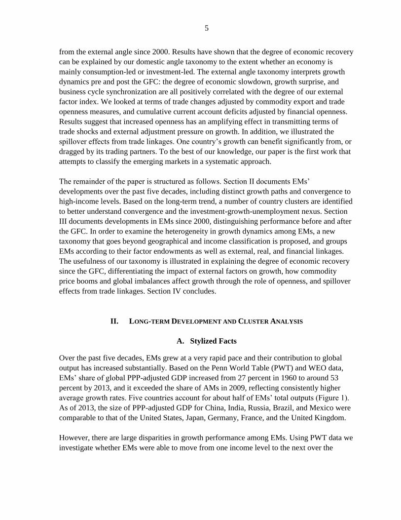
Over the past five decades, EMs grew at a very rapid pace and their contribution to global

output has increased substantially. Based on the Penn World Table (PWT) and WEO data,

EMs’ share of global PPP-adjusted GDP increased from 27 percent in 1960 to around 53

percent by 2013, and it exceeded the share of AMs in 2009, reflecting consistently higher

average growth rates. Five countries account for about half of EMs’ total outputs (Figure 1).

As of 2013, the size of PPP-adjusted GDP for China, India, Russia, Brazil, and Mexico were

comparable to that of the United States, Japan, Germany, France, and the United Kingdom.

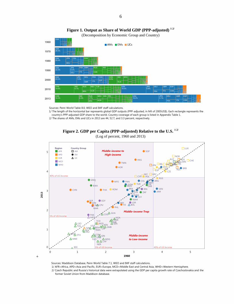
However, there are large disparities in growth performance among EMs. Using PWT data we

investigate whether EMs were able to move from one income level to the next over the

6

Figure 1. Output as Share of World GDP (PPP-adjusted) 1 2/

(Decomposition by Economic Group and Country)

Sources: Penn World Table 8.0, WEO and IMF staff calculations.

1/ The length of the horizontal bar represents global GDP outputs (PPP-adjusted, in Mil of 2005US$). Each rectangle represents the

country’s PPP-adjusted GDP share to the world. Country coverage of each group is listed in Appendix Table 1.

2/ The shares of AMs, EMs and LICs in 2013 are 44, 52.7, and 3.3 percent, respectively.

Figure 2. GDP per Capita (PPP-adjusted) Relative to the U.S. 1 2/

(Log of percent, 1960 and 2013)

+

Sources: Maddison Database, Penn World Table 7.1, WEO and IMF staff calculations.

1/ AFR=Africa, APD=Asia and Pacific, EUR=Europe, MCD=Middle East and Central Asia, WHD=Western Hemisphere.

2/ Czech Republic and Russia’s historical data were extrapolated using the GDP per capita growth rate of Czechoslovakia and the

former Soviet Union from Maddison database.

0%

20%

40%

60%

80%

100%

1960 1965 1970 1975 1980 1985 1990 1995 2000 2005 2010

Share of GDP (PPP) to World by Economy Group

AMs EMs LICs

Source: Penn World 8.0, WEO and IMF staff calculations.

1/ The sharp increases of EMs' share in 1970 and 1990 were due to the data availability changes.

2/ The shares in 2013 are 44%, 52.7% and 3.3% for AMs, EMs and LICs, respectively

7

period of 1960–2013. 3 Our analysis, which is largely consistent with the latest World Bank

classification of income groups,4 suggests that only a few EMs were able to advance to high-

income status, while many have been stuck in a middle income trap since the 1960s.

Figure 2 indicates that EMs—irrespective of geographical location—did not behave in a

consistent manner in terms of their convergence dynamics. For example, 64 percent of the

EMs, originating from all regions, are stuck in the so called “middle-income trap”, while a

few economies in Asia and Europe have successfully transformed into high-income

countries, including the “the Four Asian Tigers”.

B. Cluster Methodology and Results

The question that arises is what explains this divergent performance? To answer this question

we have applied cluster analysis to identify the patterns of economic performance among the

EM universe. A total of 25 major EMs are selected for our cluster analysis based on their

economic size, growth rate and data availability during 1980–2013.5 Using WEO 2014 data

we identify clusters for our sample using Ward’s linkage method.6 Four clusters are chosen

based on the sensitivity test.

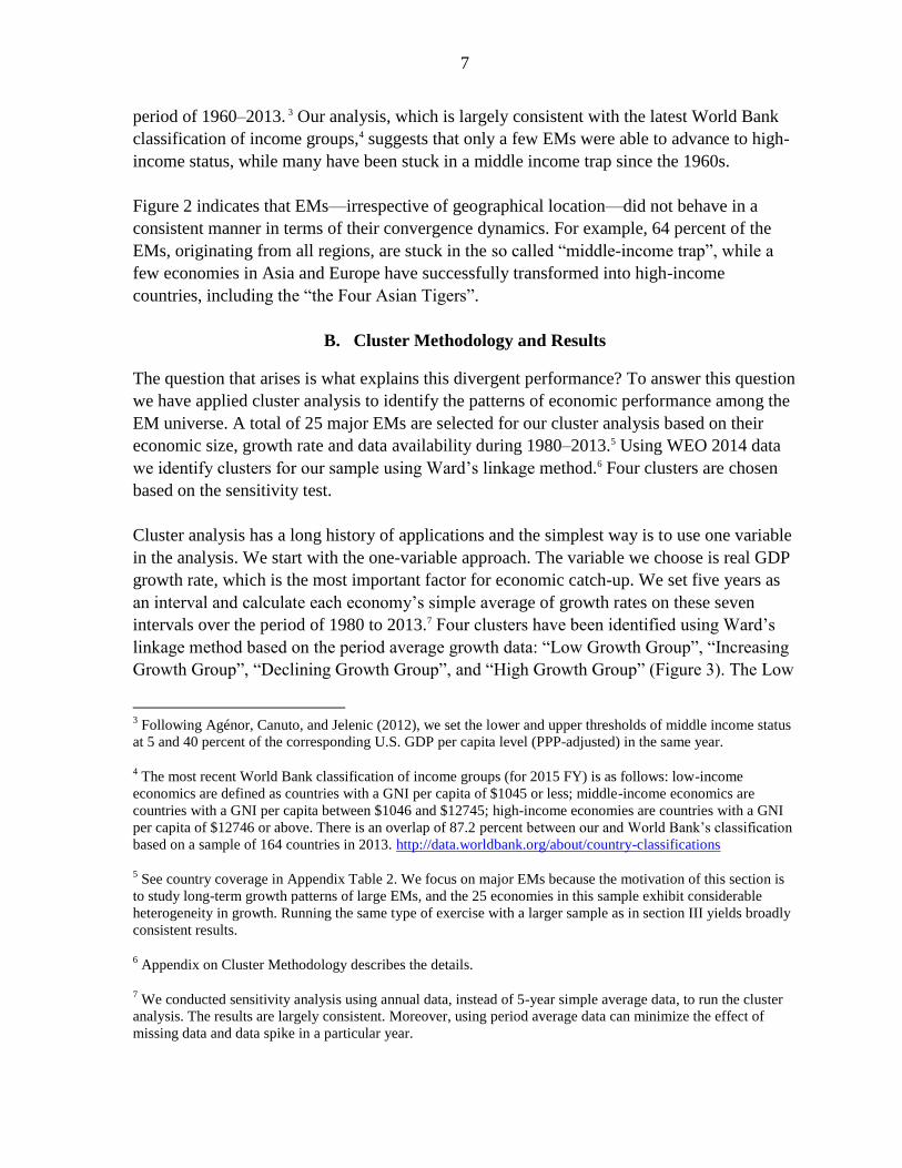
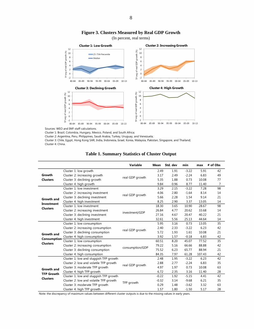
Cluster analysis has a long history of applications and the simplest way is to use one variable

in the analysis. We start with the one-variable approach. The variable we choose is real GDP

growth rate, which is the most important factor for economic catch-up. We set five years as

an interval and calculate each economy’s simple average of growth rates on these seven

intervals over the period of 1980 to 2013.7 Four clusters have been identified using Ward’s

linkage method based on the period average growth data: “Low Growth Group”, “Increasing

Growth Group”, “Declining Growth Group”, and “High Growth Group” (Figure 3). The Low

3 Following Agénor, Canuto, and Jelenic (2012), we set the lower and upper thresholds of middle income status

at 5 and 40 percent of the corresponding U.S. GDP per capita level (PPP-adjusted) in the same year.

4 The most recent World Bank classification of income groups (for 2015 FY) is as follows: low-income

economics are defined as countries with a GNI per capita of $1045 or less; middle-income economics are

countries with a GNI per capita between $1046 and $12745; high-income economies are countries with a GNI

per capita of $12746 or above. There is an overlap of 87.2 percent between our and World Bank’s classification

based on a sample of 164 countries in 2013. http://data.worldbank.org/about/country-classifications

5 See country coverage in Appendix Table 2. We focus on major EMs because the motivation of this section is

to study long-term growth patterns of large EMs, and the 25 economies in this sample exhibit considerable

heterogeneity in growth. Running the same type of exercise with a larger sample as in section III yields broadly

consistent results.

6 Appendix on Cluster Methodology describes the details.

7 We conducted sensitivity analysis using annual data, instead of 5-year simple average data, to run the cluster

analysis. The results are largely consistent. Moreover, using period average data can minimize the effect of

missing data and data spike in a particular year.

8

Figure 3. Clusters Measured by Real GDP Growth

(In percent, real terms)

Sources: WEO and IMF staff calculations. Cluster 1: Brazil, Colombia, Hungary, Mexico, Poland, and South Africa;

Cluster 2: Argentina, Peru, Philippines, Saudi Arabia, Turkey, Uruguay, and Venezuela;

Cluster 3: Chile, Egypt, Hong Kong SAR, India, Indonesia, Israel, Korea, Malaysia, Pakistan, Singapore, and Thailand;

Cluster 4: China.

Table 1. Summary Statistics of Cluster Output

Note: the discrepancy of maximum values between different cluster outputs is due to the missing values in early years.

-2

0

2

4

6

8

10

12

80-84 85-89 90-94 95-99 00-04 05-09 10-13

5Y

avg

of

real G

DP

gro

wth

(%

)

Cluster 1: Low Growth

25-75th Percentile

Median

-2

0

2

4

6

8

10

12

80-84 85-89 90-94 95-99 00-04 05-09 10-13

5Y a

vg o

f re

al G

DP g

row

th (

%)

Cluster 2: Increasing Growth

-2

0

2

4

6

8

10

12

80-84 85-89 90-94 95-99 00-04 05-09 10-13

5Y a

vg o

f re

al G

DP g

row

th (

%)

Cluster 3: Declining Growth

-2

0

2

4

6

8

10

12

80-84 85-89 90-94 95-99 00-04 05-09 10-13

5Y a

vg o

f re

al G

DP g

row

th (

%)

Cluster 4: High Growth

Variable Mean Std. dev min max # of Obs

Cluster 1: low growth 2.49 1.91 -3.22 5.91 42

Cluster 2: increasing growth 3.17 2.49 -2.24 6.83 49

Cluster 3: declining growth 5.35 1.88 0.73 10.08 77

Cluster 4: high growth 9.84 0.96 8.77 11.40 7

Cluster 1: low investment 3.29 2.15 -3.22 7.28 98

Cluster 2: increasing investment 4.06 2.80 -1.64 8.14 14

Cluster 3: declining investment 5.66 2.28 1.54 9.14 21

Cluster 4: high investment 8.25 2.90 3.37 13.05 14

Cluster 1: low investment 18.30 3.65 10.90 28.67 98

Cluster 2: increasing investment 26.84 4.77 20.62 33.68 14

Cluster 3: declining investment 27.16 4.67 20.47 40.22 21

Cluster 4: high investment 32.61 5.56 25.13 44.64 14

Cluster 1: low consumption 5.95 3.16 0.73 13.05 35

Cluster 2: increasing consumption 2.40 2.33 -3.22 6.23 42

Cluster 3: declining consumption 5.72 1.93 1.61 10.08 21

Cluster 4: high consumption 3.92 1.57 -0.18 6.83 42

Cluster 1: low consumption 60.51 8.20 45.07 77.52 35

Cluster 2: increasing consumption 79.22 5.16 66.66 88.88 42

Cluster 3: declining consumption 75.52 6.23 65.77 88.94 21

Cluster 4: high consumption 84.35 7.97 61.28 107.43 42

Cluster 1: low and sluggish TFP growth 2.48 1.95 -3.22 6.23 42

Cluster 2: low and volatile TFP growth 2.88 2.77 -2.24 6.83 35

Cluster 3: moderate TFP growth 4.97 1.97 0.73 10.08 63

Cluster 4: high TFP growth 6.72 2.35 3.16 11.40 28

Cluster 1: low and sluggish TFP growth -0.22 1.92 -5.15 4.41 42

Cluster 2: low and volatile TFP growth -0.32 3.14 -9.68 6.21 35

Cluster 3: moderate TFP growth 0.29 1.48 -3.62 3.32 63

Cluster 4: high TFP growth 1.57 1.80 -1.50 5.17 28

Growth and

TFP Growth

Clusters

real GDP growth

TFP growth

Growth

Clusters

Growth and

Investment

Clusters

Growth and

Consumption

Clusters

real GDP growth

real GDP growth

investment/GDP

real GDP growth

consumption/GDP

9

Growth Group is comprised of six countries, and they have a relatively low growth rate,

around 2.5 percent on an annual basis (Table 1). The Increasing Growth Group, which

includes seven countries, began with a slow growth pace. It has seen growth acceleration in

the later stage, although there is a large amount of variation in growth rates. In contrast, the

Declining Growth Group, which includes eleven economies, began with a fast growth pace,

then its growth declined gradually and stabilized around 4 percent on an annual basis. The

moderate shift in trend growth is accompanied by smaller dispersion in growth rates,

compared to the Increasing Growth Group. China is the only country in the High Growth

Group because China’s growth rate is exceptionally high compared to its peers through the

sample period. If we force the cluster number to be two, cluster 1 and 2 will be combined

into one group, and cluster 3 and 4 will be merged into another group.

The above results show how each group performs measured by output growth. However, it is

not clear what the driving factors are behind the fast or slow GDP growth, and whether

countries that belong to the same cluster share similarities in their growth components.

Therefore, in the second stage, we employ two measure variables in the cluster analysis. In

addition to the real GDP growth rate, we add the investment share in percent of GDP, the

consumption share in percent of GDP, and Total Factor Productivity (TFP) growth rate

separately. This enables us to understand the interaction between the total output and its main

contributing factors.8

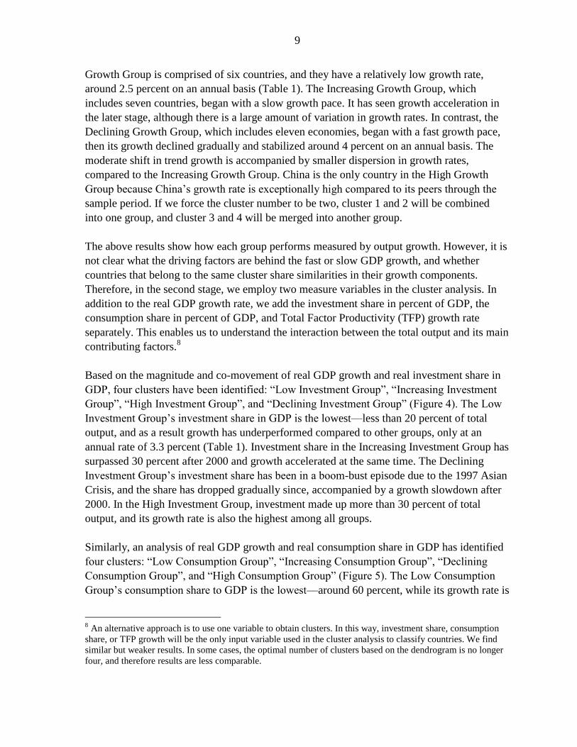
Based on the magnitude and co-movement of real GDP growth and real investment share in

GDP, four clusters have been identified: “Low Investment Group”, “Increasing Investment

Group”, “High Investment Group”, and “Declining Investment Group” (Figure 4). The Low

Investment Group’s investment share in GDP is the lowest––less than 20 percent of total

output, and as a result growth has underperformed compared to other groups, only at an

annual rate of 3.3 percent (Table 1). Investment share in the Increasing Investment Group has

surpassed 30 percent after 2000 and growth accelerated at the same time. The Declining

Investment Group’s investment share has been in a boom-bust episode due to the 1997 Asian

Crisis, and the share has dropped gradually since, accompanied by a growth slowdown after

2000. In the High Investment Group, investment made up more than 30 percent of total

output, and its growth rate is also the highest among all groups.

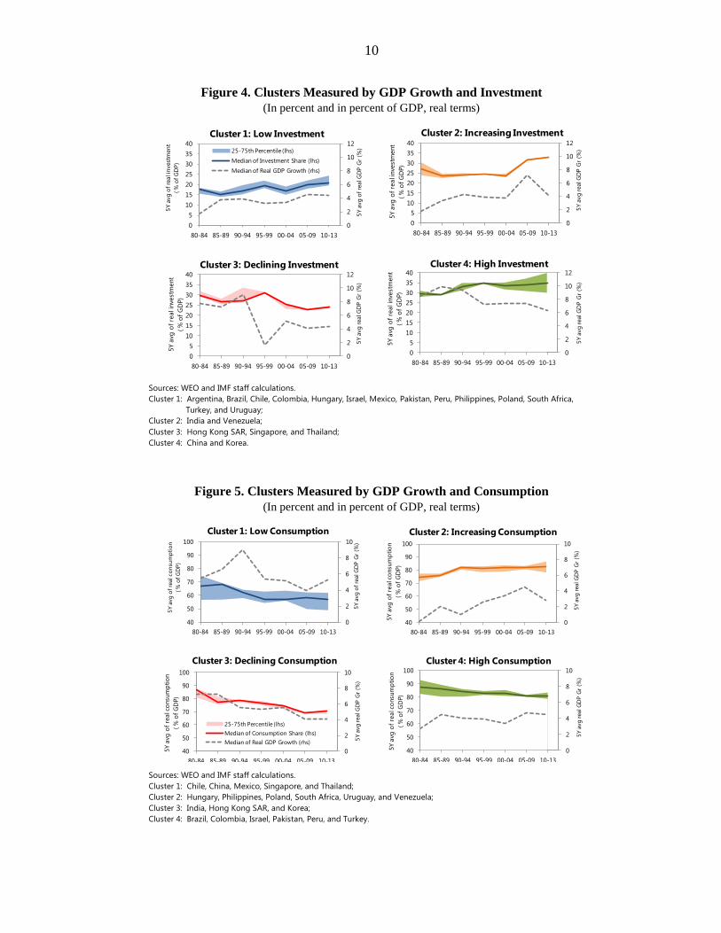
Similarly, an analysis of real GDP growth and real consumption share in GDP has identified

four clusters: “Low Consumption Group”, “Increasing Consumption Group”, “Declining

Consumption Group”, and “High Consumption Group” (Figure 5). The Low Consumption

Group’s consumption share to GDP is the lowest––around 60 percent, while its growth rate is

8 An alternative approach is to use one variable to obtain clusters. In this way, investment share, consumption

share, or TFP growth will be the only input variable used in the cluster analysis to classify countries. We find

similar but weaker results. In some cases, the optimal number of clusters based on the dendrogram is no longer

four, and therefore results are less comparable.

10

Figure 4. Clusters Measured by GDP Growth and Investment

(In percent and in percent of GDP, real terms)

Sources: WEO and IMF staff calculations.

Cluster 1: Argentina, Brazil, Chile, Colombia, Hungary, Israel, Mexico, Pakistan, Peru, Philippines, Poland, South Africa,

Turkey, and Uruguay;

Cluster 2: India and Venezuela;

Cluster 3: Hong Kong SAR, Singapore, and Thailand;

Cluster 4: China and Korea.

Figure 5. Clusters Measured by GDP Growth and Consumption

(In percent and in percent of GDP, real terms)

Sources: WEO and IMF staff calculations.

Cluster 1: Chile, China, Mexico, Singapore, and Thailand;

Cluster 2: Hungary, Philippines, Poland, South Africa, Uruguay, and Venezuela;

Cluster 3: India, Hong Kong SAR, and Korea;

Cluster 4: Brazil, Colombia, Israel, Pakistan, Peru, and Turkey.

0

2

4

6

8

10

12

0

5

10

15

20

25

30

35

40

80-84 85-89 90-94 95-99 00-04 05-09 10-13

5Y

avg

of

real G

DP

Gr

(%)

5Y

avg

of

real in

vest

men

t

( %

of

GD

P)

Cluster 1: Low Investment

25-75th Percentile (lhs)

Median of Investment Share (lhs)

Median of Real GDP Growth (rhs)

0

2

4

6

8

10

12

0

5

10

15

20

25

30

35

40

80-84 85-89 90-94 95-99 00-04 05-09 10-13

5Y

avg

real G

DP

Gr

(%)

5Y a

vg o

f re

al i

nve

stm

ent

( %

of

GD

P)

Cluster 2: Increasing Investment

0

2

4

6

8

10

12

0

5

10

15

20

25

30

35

40

80-84 85-89 90-94 95-99 00-04 05-09 10-13

5Y

avg

real G

DP

Gr

(%)

5Y a

vg o

f re

al i

nve

stm

ent

( %

of

GD

P)

Cluster 4: High Investment

0

2

4

6

8

10

12

0

5

10

15

20

25

30

35

40

80-84 85-89 90-94 95-99 00-04 05-09 10-13

5Y

avg

real G

DP

Gr

(%)

5Y a

vg o

f re

al i

nve

stm

ent

( %

of

GD

P)

Cluster 3: Declining Investment

0

2

4

6

8

10

40

50

60

70

80

90

100

80-84 85-89 90-94 95-99 00-04 05-09 10-13

5Y

avg

of

real G

DP

Gr

(%)

5Y

avg

of

real co

nsu

mp

tio

n

( %

of

GD

P)

Cluster 1: Low Consumption

0

2

4

6

8

10

40

50

60

70

80

90

100

80-84 85-89 90-94 95-99 00-04 05-09 10-13

5Y

avg

real G

DP

Gr

(%)

5Y a

vg o

f re

al c

onsu

mp

tio

n

( %

of

GD

P)

Cluster 3: Declining Consumption

25-75th Percentile (lhs)

Median of Consumption Share (lhs)

Median of Real GDP Growth (rhs)

0

2

4

6

8

10

40

50

60

70

80

90

100

80-84 85-89 90-94 95-99 00-04 05-09 10-13

5Y

avg

real G

DP

Gr

(%)

5Y a

vg o

f re

al c

onsu

mp

tio

n

( %

of

GD

P)

Cluster 2: Increasing Consumption

0

2

4

6

8

10

40

50

60

70

80

90

100

80-84 85-89 90-94 95-99 00-04 05-09 10-13

5Y

avg

real G

DP

Gr

(%)

5Y a

vg o

f re

al c

onsu

mp

tio

n

( %

of

GD

P)

Cluster 4: High Consumption

11

relatively high, especially before 2000 (Table 1). The Declining Consumption Group has

seen both consumption share and growth rate gradually decline over time. Consumption

share in the Increasing Consumption Group has risen gradually to more than 80 percent, and

growth rate has been the most disappointing though it accelerated moderately in recent years.

For the High Consumption Group, the consumption share is around 85 percent, and growth

rate remains stable around 4 percent.

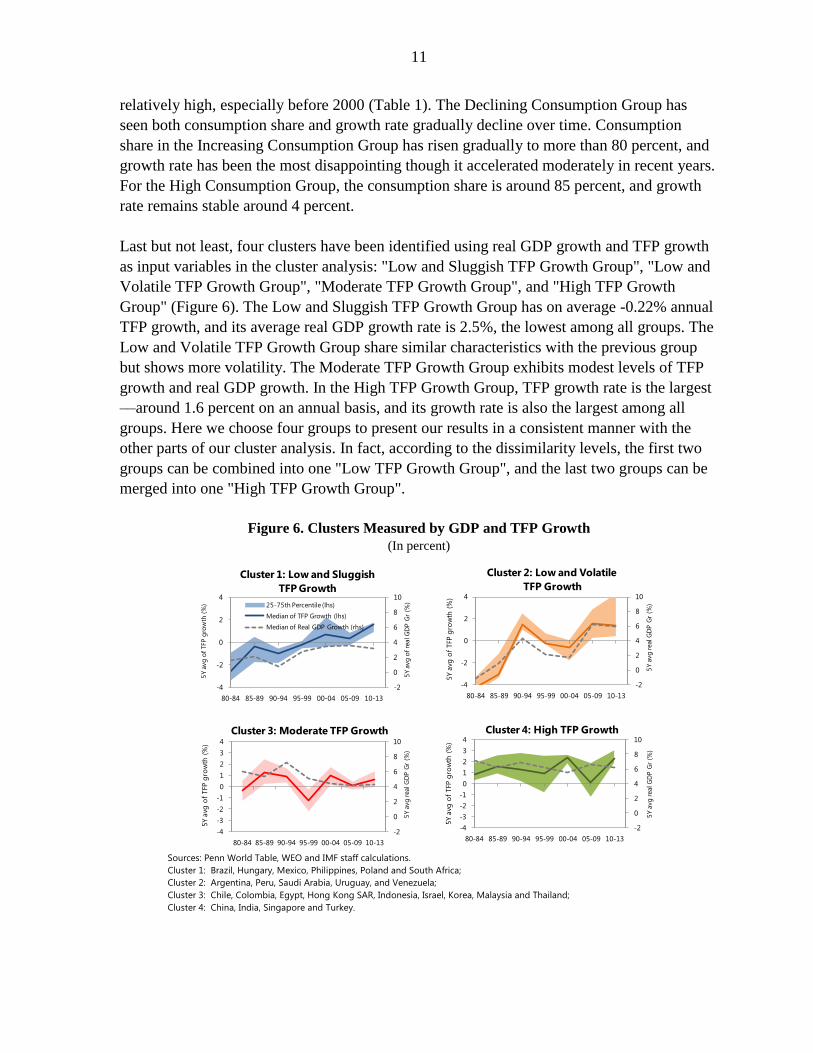
Last but not least, four clusters have been identified using real GDP growth and TFP growth

as input variables in the cluster analysis: "Low and Sluggish TFP Growth Group", "Low and

Volatile TFP Growth Group", "Moderate TFP Growth Group", and "High TFP Growth

Group" (Figure 6). The Low and Sluggish TFP Growth Group has on average -0.22% annual

TFP growth, and its average real GDP growth rate is 2.5%, the lowest among all groups. The

Low and Volatile TFP Growth Group share similar characteristics with the previous group

but shows more volatility. The Moderate TFP Growth Group exhibits modest levels of TFP

growth and real GDP growth. In the High TFP Growth Group, TFP growth rate is the largest

––around 1.6 percent on an annual basis, and its growth rate is also the largest among all

groups. Here we choose four groups to present our results in a consistent manner with the

other parts of our cluster analysis. In fact, according to the dissimilarity levels, the first two

groups can be combined into one "Low TFP Growth Group", and the last two groups can be

merged into one "High TFP Growth Group".

Figure 6. Clusters Measured by GDP and TFP Growth

(In percent)

Sources: Penn World Table, WEO and IMF staff calculations.

Cluster 1: Brazil, Hungary, Mexico, Philippines, Poland and South Africa;

Cluster 2: Argentina, Peru, Saudi Arabia, Uruguay, and Venezuela;

Cluster 3: Chile, Colombia, Egypt, Hong Kong SAR, Indonesia, Israel, Korea, Malaysia and Thailand;

Cluster 4: China, India, Singapore and Turkey.

-2

0

2

4

6

8

10

-4

-2

0

2

4

80-84 85-89 90-94 95-99 00-04 05-09 10-13

5Y

avg

of

real G

DP

Gr

(%)

5Y

avg

of

TFP

gro

wth

(%

)

Cluster 1: Low and Sluggish

TFP Growth

25-75th Percentile (lhs)

Median of TFP Growth (lhs)

Median of Real GDP Growth (rhs)

-2

0

2

4

6

8

10

-4

-2

0

2

4

80-84 85-89 90-94 95-99 00-04 05-09 10-13

5Y

avg

real G

DP

Gr

(%)

5Y a

vg o

f TFP

gro

wth

(%

)

Cluster 2: Low and Volatile

TFP Growth

-2

0

2

4

6

8

10

-4

-3

-2

-1

0

1

2

3

4

80-84 85-89 90-94 95-99 00-04 05-09 10-13

5Y

avg

real G

DP

Gr

(%)

5Y a

vg o

f TFP

gro

wth

(%

)

Cluster 4: High TFP Growth

-2

0

2

4

6

8

10

-4

-3

-2

-1

0

1

2

3

4

80-84 85-89 90-94 95-99 00-04 05-09 10-13

5Y

avg

real G

DP

Gr

(%)

5Y a

vg o

f TFP

gro

wth

(%

)

Cluster 3: Moderate TFP Growth

12

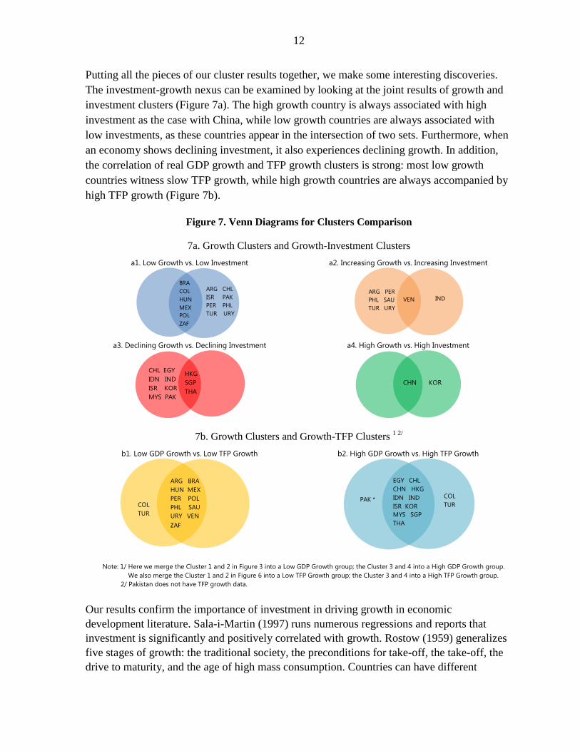
Putting all the pieces of our cluster results together, we make some interesting discoveries.

The investment-growth nexus can be examined by looking at the joint results of growth and

investment clusters (Figure 7a). The high growth country is always associated with high

investment as the case with China, while low growth countries are always associated with

low investments, as these countries appear in the intersection of two sets. Furthermore, when

an economy shows declining investment, it also experiences declining growth. In addition,

the correlation of real GDP growth and TFP growth clusters is strong: most low growth

countries witness slow TFP growth, while high growth countries are always accompanied by

high TFP growth (Figure 7b).

Figure 7. Venn Diagrams for Clusters Comparison

7a. Growth Clusters and Growth-Investment Clusters

a1. Low Growth vs. Low Investment a2. Increasing Growth vs. Increasing Investment

a3. Declining Growth vs. Declining Investment a4. High Growth vs. High Investment

7b. Growth Clusters and Growth-TFP Clusters 1 2/

b1. Low GDP Growth vs. Low TFP Growth b2. High GDP Growth vs. High TFP Growth

Note: 1/ Here we merge the Cluster 1 and 2 in Figure 3 into a Low GDP Growth group; the Cluster 3 and 4 into a High GDP Growth group.

We also merge the Cluster 1 and 2 in Figure 6 into a Low TFP Growth group; the Cluster 3 and 4 into a High TFP Growth group.

2/ Pakistan does not have TFP growth data.

Our results confirm the importance of investment in driving growth in economic

development literature. Sala-i-Martin (1997) runs numerous regressions and reports that

investment is significantly and positively correlated with growth. Rostow (1959) generalizes

five stages of growth: the traditional society, the preconditions for take-off, the take-off, the

drive to maturity, and the age of high mass consumption. Countries can have different

BRA

COL

HUN

MEX

POL

ZAF

ARG CHL

ISR PAK

PER PHL

TUR URY

VEN INDARG PER

PHL SAU

TUR URY

HKG

SGP

THA

CHL EGY

IDN IND

ISR KOR

MYS PAK

CHN KOR

COL

TUR

ARG BRA

HUN MEX

PER POL

PHL SAU

URY VEN

ZAF

COL

TUR

EGY CHL

CHN HKG

IDN IND

ISR KOR

MYS SGP

THA

PAK *

13

theoretical equilibrium positions for output and investment because they are situating in

various stages of growth, or transitioning towards new stages of growth. Based on our

results, one can check a particular country’s position in each cluster output.

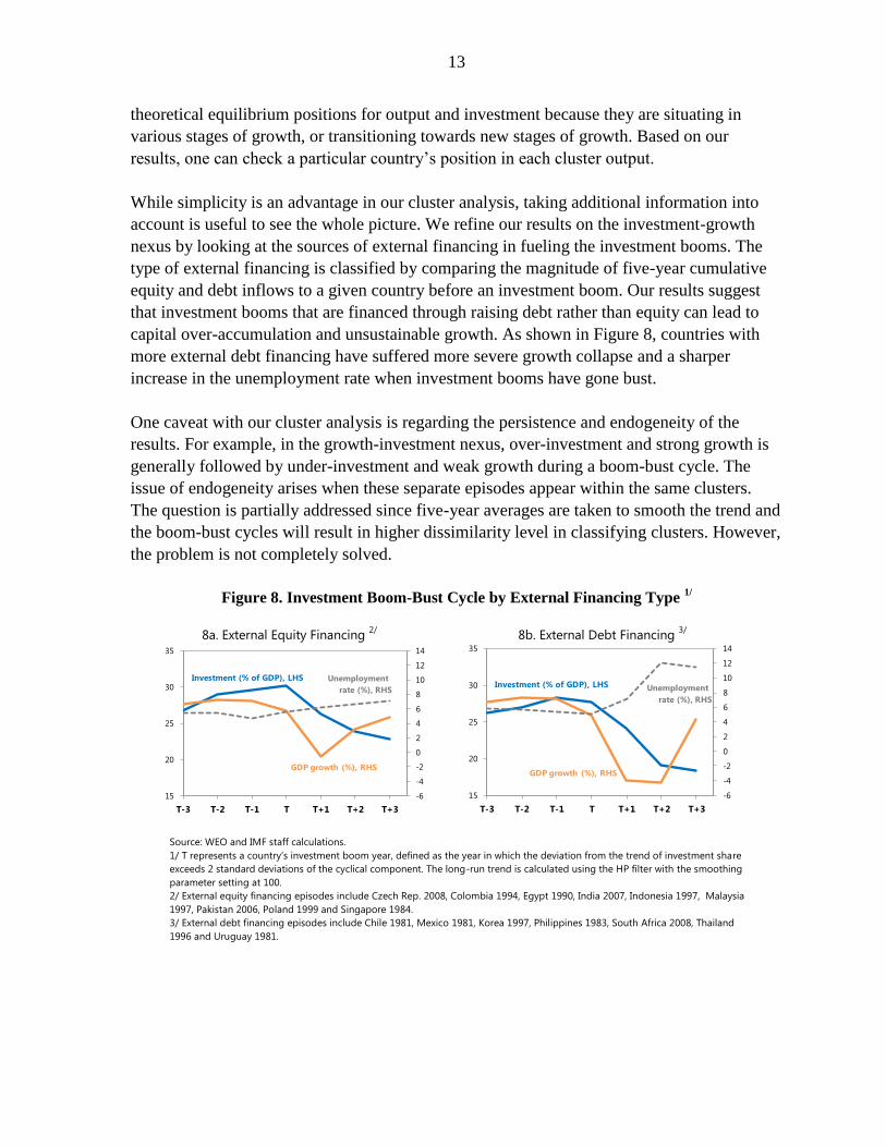
While simplicity is an advantage in our cluster analysis, taking additional information into

account is useful to see the whole picture. We refine our results on the investment-growth

nexus by looking at the sources of external financing in fueling the investment booms. The

type of external financing is classified by comparing the magnitude of five-year cumulative

equity and debt inflows to a given country before an investment boom. Our results suggest

that investment booms that are financed through raising debt rather than equity can lead to

capital over-accumulation and unsustainable growth. As shown in Figure 8, countries with

more external debt financing have suffered more severe growth collapse and a sharper

increase in the unemployment rate when investment booms have gone bust.

One caveat with our cluster analysis is regarding the persistence and endogeneity of the

results. For example, in the growth-investment nexus, over-investment and strong growth is

generally followed by under-investment and weak growth during a boom-bust cycle. The

issue of endogeneity arises when these separate episodes appear within the same clusters.

The question is partially addressed since five-year averages are taken to smooth the trend and

the boom-bust cycles will result in higher dissimilarity level in classifying clusters. However,

the problem is not completely solved.

Figure 8. Investment Boom-Bust Cycle by External Financing Type 1/

8a. External Equity Financing 2/

8b. External Debt Financing 3/

Source: WEO and IMF staff calculations.

1/ T represents a country’s investment boom year, defined as the year in which the deviation from the trend of investment share

exceeds 2 standard deviations of the cyclical component. The long-run trend is calculated using the HP filter with the smoothing

parameter setting at 100.

2/ External equity financing episodes include Czech Rep. 2008, Colombia 1994, Egypt 1990, India 2007, Indonesia 1997, Malaysia

1997, Pakistan 2006, Poland 1999 and Singapore 1984.

3/ External debt financing episodes include Chile 1981, Mexico 1981, Korea 1997, Philippines 1983, South Africa 2008, Thailand

1996 and Uruguay 1981.

-6

-4

-2

0

2

4

6

8

10

12

14

15

20

25

30

35

T-3 T-2 T-1 T T+1 T+2 T+3

Investment (% of GDP), LHS

GDP growth (%), RHS

Unemployment

rate (%), RHS

-6

-4

-2

0

2

4

6

8

10

12

14

15

20

25

30

35

T-3 T-2 T-1 T T+1 T+2 T+3

Investment (% of GDP), LHS

GDP growth (%), RHS

Unemployment

rate (%), RHS

14

C. Refining Economic Convergence Classification

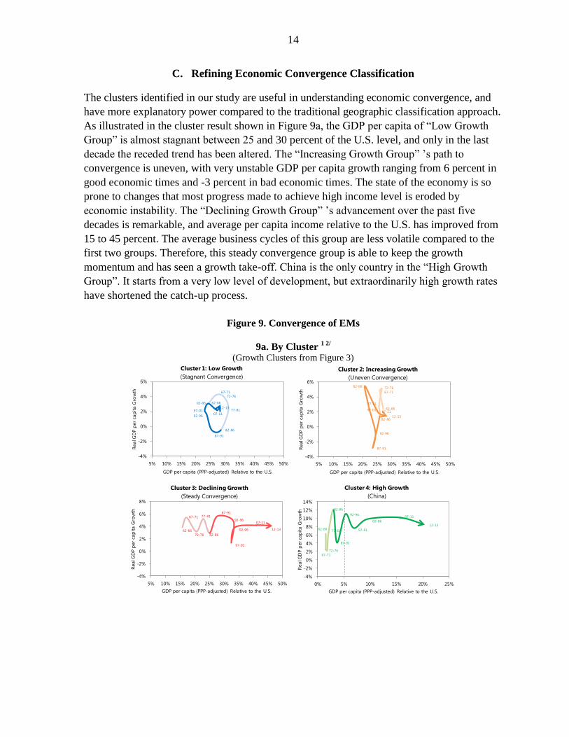
The clusters identified in our study are useful in understanding economic convergence, and

have more explanatory power compared to the traditional geographic classification approach.

As illustrated in the cluster result shown in Figure 9a, the GDP per capita of “Low Growth

Group” is almost stagnant between 25 and 30 percent of the U.S. level, and only in the last

decade the receded trend has been altered. The “Increasing Growth Group” ’s path to

convergence is uneven, with very unstable GDP per capita growth ranging from 6 percent in

good economic times and -3 percent in bad economic times. The state of the economy is so

prone to changes that most progress made to achieve high income level is eroded by

economic instability. The “Declining Growth Group” ’s advancement over the past five

decades is remarkable, and average per capita income relative to the U.S. has improved from

15 to 45 percent. The average business cycles of this group are less volatile compared to the

first two groups. Therefore, this steady convergence group is able to keep the growth

momentum and has seen a growth take-off. China is the only country in the “High Growth

Group”. It starts from a very low level of development, but extraordinarily high growth rates

have shortened the catch-up process.

Figure 9. Convergence of EMs

9a. By Cluster 1 2/

(Growth Clusters from Figure 3)

62-66

67-71

72-76

77-81

82-86

87-91

92-96

97-01

02-06

07-11

12-13

-4%

-2%

0%

2%

4%

6%

5% 10% 15% 20% 25% 30% 35% 40% 45% 50%

Real G

DP p

er

cap

ita G

row

th

GDP per capita (PPP-adjusted) Relative to the U.S.

Cluster 1: Low Growth

(Stagnant Convergence)

62-66

67-71

72-76

77-81

82-86

87-91

92-96

97-01

02-06

07-11

12-13

-4%

-2%

0%

2%

4%

6%

5% 10% 15% 20% 25% 30% 35% 40% 45% 50%

Real G

DP p

er

cap

ita G

row

th

GDP per capita (PPP-adjusted) Relative to the U.S.

Cluster 2: Increasing Growth

(Uneven Convergence)

62-66

67-71

72-76

77-81

82-86

87-91

92-96

97-01

02-06

07-11

12-13

-4%

-2%

0%

2%

4%

6%

8%

5% 10% 15% 20% 25% 30% 35% 40% 45% 50%

Real G

DP p

er

cap

ita G

row

th

GDP per capita (PPP-adjusted) Relative to the U.S.

Cluster 3: Declining Growth

(Steady Convergence)

62-66

67-71

72-76

77-81

82-86

87-91

92-96

97-01

02-06

07-11

12-13

-4%

-2%

0%

2%

4%

6%

8%

10%

12%

14%

0% 5% 10% 15% 20% 25%

Real G

DP p

er

cap

ita G

row

th

GDP per capita (PPP-adjusted) Relative to the U.S.

Cluster 4: High Growth

(China)

15

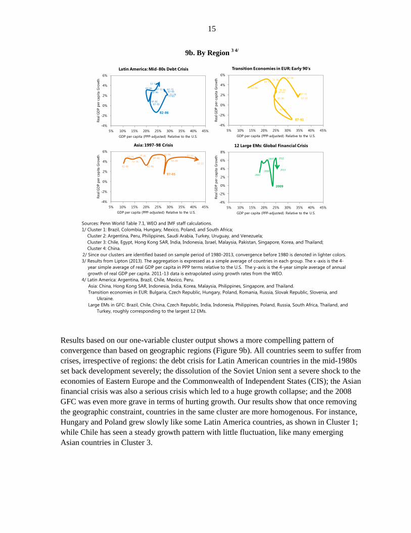
9b. By Region 3 4/

Sources: Penn World Table 7.1, WEO and IMF staff calculations.

1/ Cluster 1: Brazil, Colombia, Hungary, Mexico, Poland, and South Africa;

Cluster 2: Argentina, Peru, Philippines, Saudi Arabia, Turkey, Uruguay, and Venezuela;

Cluster 3: Chile, Egypt, Hong Kong SAR, India, Indonesia, Israel, Malaysia, Pakistan, Singapore, Korea, and Thailand;

Cluster 4: China.

2/ Since our clusters are identified based on sample period of 1980-2013, convergence before 1980 is denoted in lighter colors. 3/ Results from Lipton (2013). The aggregation is expressed as a simple average of countries in each group. The x-axis is the 4-

year simple average of real GDP per capita in PPP terms relative to the U.S. The y-axis is the 4-year simple average of annual

growth of real GDP per capita. 2011-13 data is extrapolated using growth rates from the WEO.

4/ Latin America: Argentina, Brazil, Chile, Mexico, Peru.

Asia: China, Hong Kong SAR, Indonesia, India, Korea, Malaysia, Philippines, Singapore, and Thailand.

Transition economies in EUR: Bulgaria, Czech Republic, Hungary, Poland, Romania, Russia, Slovak Republic, Slovenia, and

Ukraine.

Large EMs in GFC: Brazil, Chile, China, Czech Republic, India, Indonesia, Philippines, Poland, Russia, South Africa, Thailand, and

Turkey, roughly corresponding to the largest 12 EMs.

Results based on our one-variable cluster output shows a more compelling pattern of

convergence than based on geographic regions (Figure 9b). All countries seem to suffer from

crises, irrespective of regions: the debt crisis for Latin American countries in the mid-1980s

set back development severely; the dissolution of the Soviet Union sent a severe shock to the

economies of Eastern Europe and the Commonwealth of Independent States (CIS); the Asian

financial crisis was also a serious crisis which led to a huge growth collapse; and the 2008

GFC was even more grave in terms of hurting growth. Our results show that once removing

the geographic constraint, countries in the same cluster are more homogenous. For instance,

Hungary and Poland grew slowly like some Latin America countries, as shown in Cluster 1;

while Chile has seen a steady growth pattern with little fluctuation, like many emerging

Asian countries in Cluster 3.

62-66

67-71

72-76

77-81

82-86

87-91

92-96

97-01

02-06

07-11

12-13

-4%

-2%

0%

2%

4%

6%

5% 10% 15% 20% 25% 30% 35% 40% 45%

Real G

DP p

er

cap

ita G

row

th

GDP per capita (PPP-adjusted) Relative to the U.S.

Asia: 1997-98 Crisis

62-6667-71

72-7677-81

82-86

87-91

92-96

97-01

02-06 07-11

12-13

-4%

-2%

0%

2%

4%

6%

5% 10% 15% 20% 25% 30% 35% 40% 45%

Real G

DP p

er

cap

ita G

row

th

GDP per capita (PPP-adjusted) Relative to the U.S.

Latin America: Mid-80s Debt Crisis

62-66

67-7172-76

77-81

82-86

87-91

92-96

97-01

02-06

07-11

12-13

-4%

-2%

0%

2%

4%

6%

5% 10% 15% 20% 25% 30% 35% 40% 45%

Real G

DP p

er

cap

ita G

row

th

GDP per capita (PPP-adjusted) Relative to the U.S.

Transition Economies in EUR: Early 90's

2002

2007

2008

2009

2011

2013

-4%

-2%

0%

2%

4%

6%

8%

5% 10% 15% 20% 25% 30% 35% 40% 45%

Real G

DP p

er

cap

ita G

row

thGDP per capita (PPP-adjusted) Relative to the U.S.

12 Large EMs: Global Financial Crisis

16

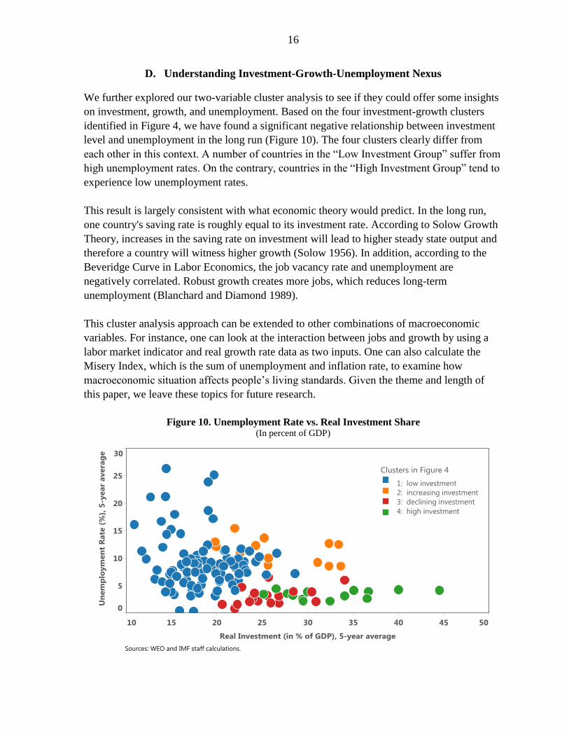
D. Understanding Investment-Growth-Unemployment Nexus

We further explored our two-variable cluster analysis to see if they could offer some insights

on investment, growth, and unemployment. Based on the four investment-growth clusters

identified in Figure 4, we have found a significant negative relationship between investment

level and unemployment in the long run (Figure 10). The four clusters clearly differ from

each other in this context. A number of countries in the “Low Investment Group” suffer from

high unemployment rates. On the contrary, countries in the “High Investment Group” tend to

experience low unemployment rates.

This result is largely consistent with what economic theory would predict. In the long run,

one country's saving rate is roughly equal to its investment rate. According to Solow Growth

Theory, increases in the saving rate on investment will lead to higher steady state output and

therefore a country will witness higher growth (Solow 1956). In addition, according to the

Beveridge Curve in Labor Economics, the job vacancy rate and unemployment are

negatively correlated. Robust growth creates more jobs, which reduces long-term

unemployment (Blanchard and Diamond 1989).

This cluster analysis approach can be extended to other combinations of macroeconomic

variables. For instance, one can look at the interaction between jobs and growth by using a

labor market indicator and real growth rate data as two inputs. One can also calculate the

Misery Index, which is the sum of unemployment and inflation rate, to examine how

macroeconomic situation affects people’s living standards. Given the theme and length of

this paper, we leave these topics for future research.

Figure 10. Unemployment Rate vs. Real Investment Share (In percent of GDP)

Sources: WEO and IMF staff calculations.

1: low investment

2: increasing investment

3: declining investment

4: high investment

17

III. RECENT PERFORMANCE AND TAXONOMY OF EMERGING MARKETS

A. Taxonomy Methodology and Results

In this section we look at the performance of emerging markets since 2000 and propose a

novel taxonomy to classify countries according to their factor endowments as well as

external, real, and financial linkages. Unlike the aforementioned cluster analysis in section II,

our taxonomy has a short-term focus and utilizes data from 2000 onwards. This also allows

us to expand our data sample to 52 economies, including 43 major EMs and 9 Newly

Industrialized Economies, covering five different regions.9 In this section, six clusters are

identified for each indicator using Ward’s linkage method, and then the cluster numbers are

reduced to three based on the authors’ judgment and sensitivity analysis results. Kernel

density estimation is used as robustness test to ensure correctness of the countries in different

clusters.

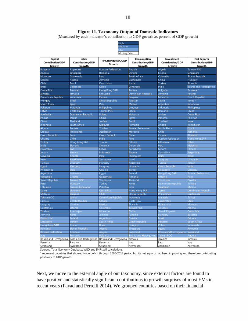
Recently, emerging markets are slowing down due to both external and domestic factors, as

shown in Cubeddu et al. (2014). This prompts us to classify the taxonomy from both

domestic and external angles. From the domestic angle of our taxonomy, we examine driving

forces of growth from the supply and demand side of the economy. From the supply side, we

decompose total real output growth into the following sources: physical capital contribution,

labor contribution, and TFP contribution. We then calculate the ratios of each component’s

contribution to total growth for each country and conduct a

cluster analysis using the median values of annual data during 2000–2013 for each country.

The taxonomy output is presented in Figure 11. The higher the rank is, the more “capital-

driven”, “labor-driven” and “technology-driven” the country is. On the demand side, we

decompose total real output growth similarly into consumption contribution, investment

contribution, and net exports contribution. We apply the same cluster methodology to

demand side indicators. The higher the rank is, the more “consumption-led”, “investment-

led” and “export-led” the country is.

9 The complete country list for taxonomy analysis is shown in Appendix Table 3. Underlying data sources are

listed in Appendix Table 4.

18

Figure 11. Taxonomy Output of Domestic Indicators (Measured by each indicator’s contribution to GDP growth as percent of GDP growth)

Sources: Total Economy Database, WEO and IMF staff calculations.

* represent countries that showed trade deficit through 2000-2012 period but its net exports had been improving and therefore contributing

positively to GDP growth.

Next, we move to the external angle of our taxonomy, since external factors are found to

have positive and statistically significant contributions to growth surprises of most EMs in

recent years (Fayad and Perrelli 2014). We grouped countries based on their financial

High

Medium

Low

Missing Data

Capital

Contribution/GDP

Growth

Labor

Contribution/GDP

Growth

TFP Contribution/GDP

Growth

Consumption

Contribution/GDP

Growth

Investment

Contribution/GDP

Growth

Net Exports

Contribution/GDP

Growth

Bulgaria Argentina Russian Federation Angola Algeria Taiwan POC

Angola Singapore Romania Ukraine Estonia Singapore

Morocco Guatemala Iraq South Africa Colombia Slovak Republic

Mexico Algeria Armenia Guatemala China Hungary

Chile Brazil Kazakhstan Jordan Turkey Slovenia

Brazil Colombia Korea Venezuela India Bosnia and Herzegovina

Costa Rica Pakistan Hong Kong SAR Tunisia Bulgaria Panama *

Jamaica Jamaica Lithuania Dominican Republic Armenia Poland

Dominican Republic Venezuela Estonia Bulgaria Morocco Czech Republic

Hungary Israel Slovak Republic Pakistan Latvia Korea *

South Africa Egypt Peru Mexico Argentina Indonesia

Pakistan Malaysia Philippines Uruguay Indonesia Philippines

Latvia Costa Rica Taiwan POC Latvia Romania China

Azerbaijan Dominican Republic Poland Malaysia Jordan Costa Rica

Poland Jordan China Egypt Panama Pakistan

China Thailand Jordan Brazil Thailand Israel

Indonesia South Africa Malaysia Romania Angola Kazakhstan

Algeria Tunisia Thailand Russian Federation South Africa Egypt

Croatia Philippines Azerbaijan Morocco Chile Armenia

Czech Republic Peru Czech Republic Chile Croatia Thailand

Ukraine Chile India Peru Russian Federation Hong Kong SAR

Turkey Hong Kong SAR Tunisia Estonia Lithuania Latvia

India Slovenia Slovenia Colombia Peru Malaysia

Colombia Iraq Latvia Kazakhstan Mexico Ukraine

Jordan Mexico Indonesia Algeria Costa Rica Argentina

Slovenia Angola Israel Philippines Brazil Brazil

Israel Kazakhstan Singapore Israel Uruguay Lithuania

Tunisia Uruguay Hungary Argentina Tunisia Jordan

Egypt Morocco Uruguay Lithuania Czech Republic India

Philippines India Ukraine Turkey Singapore Uruguay

Argentina Indonesia Egypt Poland Hong Kong SAR Russian Federation

Venezuela Croatia Guatemala Armenia Ukraine Peru

Slovak Republic Taiwan POC Venezuela Thailand Venezuela Croatia

Peru Hungary Turkey Korea Dominican Republic Tunisia

Lithuania Russian Federation Pakistan India Swaziland Mexico

Korea Lithuania Costa Rica Hong Kong SAR Korea Dominican Republic

Malaysia Bulgaria Chile Slovak Republic Philippines Guatemala

Taiwan POC Latvia Dominican Republic Indonesia Malaysia Turkey

Estonia Czech Republic Croatia Costa Rica Kazakhstan Chile

Uruguay Ukraine Mexico Slovenia Guatemala Morocco

Guatemala Estonia Colombia Taiwan POC Slovenia Algeria

Thailand Azerbaijan Morocco China Slovak Republic Colombia

Armenia Korea Jamaica Panama Hungary Bulgaria

Kazakhstan Poland Argentina Croatia Israel Estonia

Singapore Turkey South Africa Czech Republic Pakistan South Africa

Hong Kong SAR China Brazil Hungary Poland Venezuela

Romania Slovak Republic Algeria Singapore Egypt Romania

Russian Federation Armenia Angola Swaziland Bosnia and Herzegovina Swaziland

Iraq Romania Bulgaria Bosnia and Herzegovina Taiwan POC Angola

Bosnia and Herzegovina Bosnia and Herzegovina Bosnia and Herzegovina Jamaica Jamaica Jamaica

Panama Panama Panama Iraq Iraq Iraq

Swaziland Swaziland Swaziland Azerbaijan Azerbaijan Azerbaijan

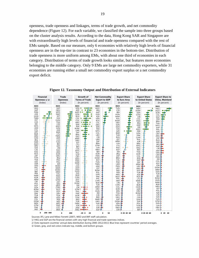
19

openness, trade openness and linkages, terms of trade growth, and net commodity

dependence (Figure 12). For each variable, we classified the sample into three groups based

on the cluster analysis results. According to the data, Hong Kong SAR and Singapore are

with extraordinarily high levels of financial and trade openness compared with the rest of

EMs sample. Based on our measure, only 6 economies with relatively high levels of financial

openness are in the top-tier in contrast to 23 economies in the bottom-tier. Distribution of

trade openness is more uniform among EMs, with about one third of economies in each

category. Distribution of terms of trade growth looks similar, but features more economies

belonging to the middle category. Only 9 EMs are large net commodity exporters, while 31

economies are running either a small net commodity export surplus or a net commodity

export deficit.

Figure 12. Taxonomy Output and Distribution of External Indicators

Sources: IFS, Lane and Milesi-Ferretti (2007), WEO and IMF staff calculation.

1/ HKG and SGP are the financial centers with very high financial and trade openness indices.

2/ Dots represent countries’ annual data distribution during 2000-2012/2013; Blue lines represent countries’ period averages.

3/ Green, grey, and red colors indicate top, middle, and bottom groups.

20

In addition, we calculated each EM's trade linkage with three major world trade partners: the

Euro area, the U.S., and China. Each taxonomy has three groups: for export to the Euro area,

cutoff points for high, medium, and low linkages are 49 percent and 29 percent; for export to

the U.S., cutoff points are 34 percent and 14 percent; for export to China, cutoff points are 12

percent and 4 percent. On average EMs have stronger trade ties with the Euro area and the

U.S. than their trade ties with China. However, this relationship is evolving as China plays an

increasingly important role in the global supply chain. We will expand this discussion later

together with Figure 16.

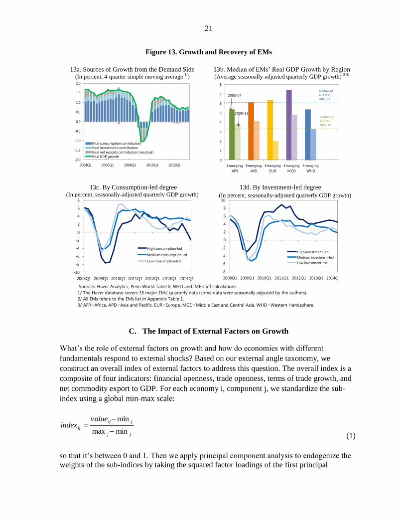
B. Explaining the Degree of Economic Recovery

Now we turn to investigate what implications our taxonomy can offer in explaining the

trends since 2000. Using our domestic angle taxonomy results, the speed and degree of

economic recovery since the GFC can be explained by our domestic angle taxonomy to the

extent whether an economy is primarily consumption-led or investment-led. When the crisis

began, EMs were hit badly, with growth rates of all output components moving towards

negative territory. This is illustrated in the growth dynamics under high frequency (Figure

13a). After global trade collapsed, EMs’ growth decomposition has shown that net exports

contributed negatively to growth for four consecutive quarters. Consumption and investment

were weak as well, adding more downward pressure on growth. The degree of EMs’

economic deteriorations were different across geographic regions (Figure 13b). Emerging

Europe had the sharpest real output decline among all regions because it has closer trade and

financial ties with AMs. Other regions were not immune to the effects of the recession.

Compared to pre-crisis growth, post-crisis growth has lowered by 4.3 percentage points for

Emerging Europe and 1.5 to 2.6 percentage points for other regions. EMs rebounded

relatively quickly overall in the post-crisis period, though recovery speed varied by

geographic region. Our taxonomy indicates that countries that are mainly consumption-led

rebounded the slowest and weakest (Figure 13c). The high consumption-led group, which

includes a set of six countries, had the deepest recession, and its recovery was the weakest

among all groups. On the other hand, countries that are mainly investment-led rebounded the

fastest and strongest (Figure 13d). The high investment-led group, which includes

another distinct set of six countries, had the mildest recession, and its recovery was the most

robust among all groups. Post-crisis growth rates of the high investment-led group have

always excelled that of the medium and low investment-led groups.10

One conjecture to

explain this phenomenon is that economic agents can adjust consumption freely based on

observed shocks, while it is more difficult to do so for investment due to capital

irreversibility and adjustment costs. Therefore investment can stabilize the economy in the

short run and promote growth in the long run.

10

We have performed robustness tests for output recovery dynamics by consumption-led and investment-led

degree in the 1980s and 1990s. The results are similar.

21

Figure 13. Growth and Recovery of EMs

13a. Sources of Growth from the Demand Side

(In percent, 4-quarter simple moving average 1/)

13b. Median of EMs’ Real GDP Growth by Region (Average seasonally-adjusted quarterly GDP growth) 2 3/

13c. By Consumption-led degree (In percent, seasonally-adjusted quarterly GDP growth)

13d. By Investment-led degree

(In percent, seasonally-adjusted quarterly GDP growth)

Sources: Haver Analytics, Penn World Table 8, WEO and IMF staff calculations.

1/ The Haver database covers 35 major EMs’ quarterly data (some data were seasonally adjusted by the authors).

2/ All EMs refers to the EMs list in Appendix Table 1.

3/ AFR=Africa, APD=Asia and Pacific, EUR=Europe, MCD=Middle East and Central Asia, WHD=Western Hemisphere.

C. The Impact of External Factors on Growth

What’s the role of external factors on growth and how do economies with different

fundamentals respond to external shocks? Based on our external angle taxonomy, we

construct an overall index of external factors to address this question. The overall index is a

composite of four indicators: financial openness, trade openness, terms of trade growth, and

net commodity export to GDP. For each economy i, component j, we standardize the sub-

index using a global min-max scale:

jj

jij

ij

valueindex

minmax

min

(1)

so that it’s between 0 and 1. Then we apply principal component analysis to endogenize the

weights of the sub-indices by taking the squared factor loadings of the first principal

-2.0

-1.5

-1.0

-0.5

0.0

0.5

1.0

1.5

2.0

2004Q1 2006Q1 2008Q1 2010Q1 2012Q1

Real consumption contribution

Real investment contribution

Real net exports contribution (residual)

Real GDP growth0

1

2

3

4

5

6

7

8

Emerging

AFR

Emerging

APD

Emerging

EUR

Emerging

MCD

Emerging

WHD

Median of EMs' Real GDP Growth By Region

(Pre v.s. Post Crisis)

1/ All EMs refers to the EM list in Annex I

Source: Penn World Table8.0 , WEO and IMF Staff Calculation

Median of

All EMs,

2008-13

2003-07

2008-13

Median of

All EMs 1/,

2003-07

-10

-8

-6

-4

-2

0

2

4

6

8

2008Q1 2009Q1 2010Q1 2011Q1 2012Q1 2013Q1 2014Q1

Growth Recovery of EMs

(Average seaonally-adjusted quarterly GDP growth)

High consumption-led

Medium consumption-led

Low consumption-led

-8

-6

-4

-2

0

2

4

6

8

10

2008Q1 2009Q1 2010Q1 2011Q1 2012Q1 2013Q1 2014Q1

Growth Recovery of EMs

(Average seaonally-adjusted quarterly GDP growth)

High investment-led

Medium investment-led

Low investment-led

22

component. Finally, a unique index will be assigned to each country by taking the weighted

averages of its four components. The higher the index is, the more the country is exposed to

the world economy. Next, we divide our sample into tertiles and examine the impact of

external factors on growth, before and after the Global Financial Crisis.

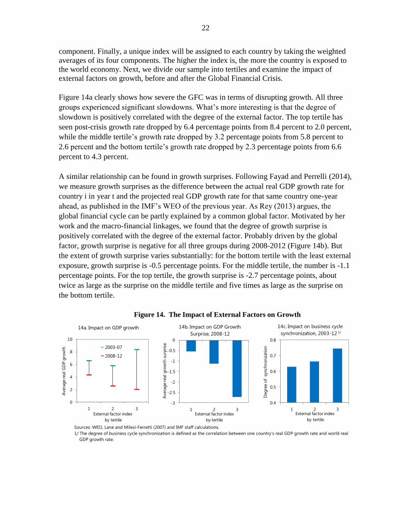
Figure 14a clearly shows how severe the GFC was in terms of disrupting growth. All three

groups experienced significant slowdowns. What’s more interesting is that the degree of

slowdown is positively correlated with the degree of the external factor. The top tertile has

seen post-crisis growth rate dropped by 6.4 percentage points from 8.4 percent to 2.0 percent,

while the middle tertile’s growth rate dropped by 3.2 percentage points from 5.8 percent to

2.6 percent and the bottom tertile’s growth rate dropped by 2.3 percentage points from 6.6

percent to 4.3 percent.

A similar relationship can be found in growth surprises. Following Fayad and Perrelli (2014),

we measure growth surprises as the difference between the actual real GDP growth rate for

country i in year t and the projected real GDP growth rate for that same country one-year

ahead, as published in the IMF’s WEO of the previous year. As Rey (2013) argues, the

global financial cycle can be partly explained by a common global factor. Motivated by her

work and the macro-financial linkages, we found that the degree of growth surprise is

positively correlated with the degree of the external factor. Probably driven by the global

factor, growth surprise is negative for all three groups during 2008-2012 (Figure 14b). But

the extent of growth surprise varies substantially: for the bottom tertile with the least external

exposure, growth surprise is -0.5 percentage points. For the middle tertile, the number is -1.1

percentage points. For the top tertile, the growth surprise is -2.7 percentage points, about

twice as large as the surprise on the middle tertile and five times as large as the surprise on

the bottom tertile.

Figure 14. The Impact of External Factors on Growth

Sources: WEO, Lane and Milesi-Ferretti (2007) and IMF staff calculations.

1/ The degree of business cycle synchronization is defined as the correlation between one country’s real GDP growth rate and world real

GDP growth rate.

0

2

4

6

8

10

1 2 3

Avera

ge r

eal

GD

P g

row

th

External factor index

by tertile

14a. Impact on GDP growth

2003-07

2008-12

-3

-2.5

-2

-1.5

-1

-0.5

0

1 2 3

Avera

ge r

eal

gro

wth

su

rpri

se

External factor index

by tertile

14b. Impact on GDP Growth

Surprise, 2008-12

0.4

0.5

0.6

0.7

0.8

1 2 3

Deg

ree o

f s

yn

ch

ron

izati

on

External factor index

by tertile

14c. Impact on business cycle

synchronization, 2003-12 1/

23

Lastly, we investigate the degree of business cycle synchronization since the assumption is

that the higher the external factor is for a given country, the more closely its business cycle

should co-move with the world economy. The result in Figure 14c supports our assumption:

the degree of business cycle synchronization is positively correlated with the degree of the

external factor. For the bottom, middle, and top tertiles, their output correlations with global

output are 0.63, 0.66, and 0.75 respectively.

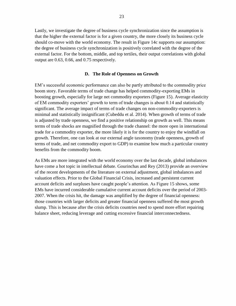
D. The Role of Openness on Growth

EM’s successful economic performance can also be partly attributed to the commodity price

boom story. Favorable terms of trade change has helped commodity-exporting EMs in

boosting growth, especially for large net commodity exporters (Figure 15). Average elasticity

of EM commodity exporters’ growth to term of trade changes is about 0.14 and statistically

significant. The average impact of terms of trade changes on non-commodity-exporters is

minimal and statistically insignificant (Cubeddu et al. 2014). When growth of terms of trade

is adjusted by trade openness, we find a positive relationship on growth as well. This means

terms of trade shocks are magnified through the trade channel: the more open in international

trade for a commodity exporter, the more likely it is for the country to enjoy the windfall on

growth. Therefore, one can look at our external angle taxonomy (trade openness, growth of

terms of trade, and net commodity export to GDP) to examine how much a particular country

benefits from the commodity boom.

As EMs are more integrated with the world economy over the last decade, global imbalances

have come a hot topic in intellectual debate. Gourinchas and Rey (2013) provide an overview

of the recent developments of the literature on external adjustment, global imbalances and

valuation effects. Prior to the Global Financial Crisis, increased and persistent current

account deficits and surpluses have caught people’s attention. As Figure 15 shows, some

EMs have incurred considerable cumulative current account deficits over the period of 2003-

2007. When the crisis hit, the damage was amplified by the degree of financial openness:

those countries with larger deficits and greater financial openness suffered the most growth

slump. This is because after the crisis deficits countries need to spend more effort repairing

balance sheet, reducing leverage and cutting excessive financial interconnectedness.

24

Figure 15. The Impacts on Growth from Commodity Boom and

Global Imbalances Adjusted by Openness Measures

Source: WDI, WEO and IMF staff calculations.

1/ Angola and Venezuela are omitted for presentation purpose given the magnitude of their x-axis variables.

2/ Hong Kong SAR and Singapore are omitted for presentation purpose given the magnitude of their financial openness.

E. Trade Linkages and Spillover Effects

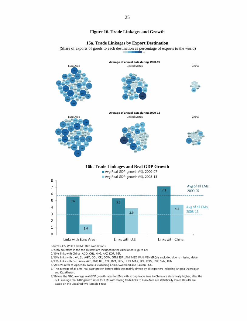
How do trading partners matter for economic growth? Figure 16a shows an increasingly

strong trade tie of EMs with China. In the 1990s, the average EMs' exports to the Euro area,

the U.S., and China as percentage of exports to the world were 27.3, 17.3, and 2.3 percent

respectively. Ten years later, average EMs' exports to the U.S., Euro area, and China became

28, 17.5, and 5.4 percent. While EMs' average export shares to Euro area and U.S. remained

strong and stable, their average export share to China has increased by 132 percent. Using the

top taxonomies which have strong trade linkages to the Euro area, the U.S., and China, we

calculated summary statistics on the simple average of real growth rates of those top

taxonomies. Results in Figure 16b indicate that countries who trade more with China on

average experienced faster growth than countries who trade more with the other two

economies. This fact was more pronounced in the post-crisis period, as the Euro area’s

trading partners have witnessed their growth almost faltering. A recent paper by Mishra et al.

(2014) has complemented our results. The authors study the market reactions of 21 emerging

markets to the U.S. Federal Reserve’s policy announcements relating to reducing its asset

purchase programs in 2013 and 2014. They find that the stronger trade linkage with China

(measured by total trade with China to its own GDP), the less market volatility a country will

experience during the Fed tapering talk, ceteris paribus.

0

2

4

6

8

10

12

-50 0 50 100 150 200

Real G

DP g

row

th

Growth of terms of trade adjusted by

net commodity export (% of GDP) 1/

0

2

4

6

8

10

12

-1,000 0 1,000 2,000

Real G

DP G

row

th

Growth of terms of trade adjusted

by trade openness

-4

-2

0

2

4

6

8

10

-20000 0 20000

Real G

DP g

row

th

Cumulative current account deficit

adjusted by financial openness 2/

(2000-10) (2000-12) (2003-07)

25

Figure 16. Trade Linkages and Growth

16a. Trade Linkages by Export Destination

(Share of exports of goods to each destination as percentage of exports to the world)

16b. Trade Linkages and Real GDP Growth

Sources: IFS, WEO and IMF staff calculations.

1/ Only countries in the top clusters are included in the calculation (Figure 12)

2/ EMs links with China: AGO, CHL, HKG, KAZ, KOR, PER

3/ EMs links with the U.S.: AGO, COL, CRI, DOM, GTM, ISR, JAM, MEX, PAN, VEN (IRQ is excluded due to missing data)

4/ EMs links with Euro Area: AZE, BGR, BIH, CZE, DZA, HRV, HUN, MAR, POL, ROM, SVK, SVN, TUN

5/ All EMs refer to Appendix Table 3, excluding China, Swaziland and Taiwan POC.

6/ The average of all EMs’ real GDP growth before crisis was mainly driven by oil exporters including Angola, Azerbaijan

and Kazakhstan.

7/ Before the GFC, average real GDP growth rates for EMs with strong trade links to China are statistically higher; after the

GFC, average real GDP growth rates for EMs with strong trade links to Euro Area are statistically lower. Results are

based on the unpaired two-sample t-test.

5.6 5.3

7.1

1.4

3.9

4.4

0

1

2

3

4

5

6

7

8

Links with Euro Area Links with U.S. Links with China

Trade Linkage and Real GDP GrowthAvg Real GDP growth (%), 2000-07

Avg Real GDP growth (%), 2008-13

Note: (1) Only countries in the top cluster are included in the calculation of growth by trade linkage(2) EMs links with China: AGO, CHL, HKG, KAZ, KOR, PER(3) EMs links with the US: AGO, COL, CRI, DOM, GTM, IRQ, ISR, JAM, MEX, PAN, VEN(4) EMs links with Euro Zone: AZE, BGR, BIH, CZE, DZA, HRV, HUN, MAR, POL, ROM, SVK, SVN, TUN(5) All EMs refer to Annex Table 3, excluding China Mainland, Swaziland and Taiwan Province of China.

Source: WEO and IMF staff calculations.

Avg of all EMs,2000-07

Avg of all EMs,2008-13

26

IV. CONCLUSIONS

Emerging market economies’ rise over the last five decades has greatly reshaped the global

economic landscape. Their contribution to world output makes them a significant economic

powerhouse that cannot be ignored. We are contributing to the literature by exploring

emerging market heterogeneity and identifying clusters and creating a simple taxonomy

based on EMs’ fundamentals. The clusters identified in our study point to four distinct

patterns of long-term economic convergence and have more explanatory power in

understanding convergence than the traditional geographic classification approach. We found

an interesting interaction between long-term growth and investment clusters: investment

clusters are highly correlated with growth clusters, and this indicates that investment is a

necessary but not sufficient condition for growth. In addition, economic growth and

productivity improvement tend to go hand in hand, according to our TFP growth and real

GDP growth clusters. On the investment-growth-unemployment nexus, on average countries

in the high investment-growth group tends to have low unemployment rates, while countries

in the low investment-growth group are likely to have high unemployment rates.

In recent years, Emerging Market Economies have seen a prolonged boom period before the

Global Financial Crisis. EMs rebounded relatively quickly overall in the post-crisis period,

but the growth has slowed recently. With the taxonomy provided in this paper, one can

examine the heterogeneity of EMs from factor endowments, external, real, and financial

linkages. Results have shown that the degree of economic recovery can be explained by the

source of growth: countries that are mainly investment-led rebounded the fastest and

strongest, while countries that are mainly consumption-led rebounded the slowest and

weakest. The external factors play an important role to explain growth dynamics pre and post

Global Financial Crisis: the degree of economic slowdown, growth surprise, and business

cycle synchronization are all positively correlated with the degree of our external factor

index. To study the impact on growth from booms in commodity prices and global

imbalances, we look at terms of trade changes adjusted by commodity export and trade

openness measures, and cumulative current account deficits adjusted by financial openness.

Results suggest that increased openness has an amplifying effect in transmitting terms of

trade shocks and external adjustment pressure on growth. In addition, we emphasized the

spillover effects from trade linkages. One country’s growth can benefit significantly from, or

dragged by its trading partners, depends on who you trade with.

Looking forward, continuing convergence to high income level for EMs will be more

challenging and is not guaranteed. Tailored policy actions are needed to take into account the

heterogeneity in the EM universe beyond the traditional geographical and income approach.

The clusters and taxonomy presented in this paper can be used as a reference to design both

near and long-term policies.

27

APPENDIX

Cluster Methodology

Ward’s method starts with n clusters (in our case n=25) of size 1 and stops when all the observations

are merged into one single cluster. In each step, the observations are combined to minimize the errors

sum of squares (or equivalently, maximize the R-square) from the group centroid. We conduct a two-

stage clustering approach in section II: in the first stage, we obtain cluster IDs for each observation

within a given country, hence a country will have a series of 7 cluster IDs in our case; in the second

stage, all the cluster IDs of each country are utilized to determine a single cluster ID for that country.

The final output is shown in the figure below. Note that the numbers of clusters is chosen at the

discretion of the dissimilarity level. We believe four is an appropriate number that distinguishes

clusters among EMs and allows good interpretation of similar characteristics within each cluster.

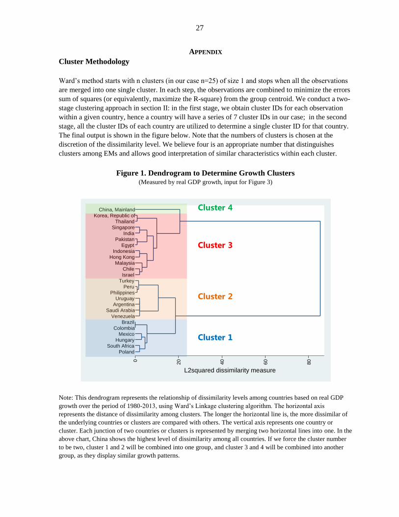
Figure 1. Dendrogram to Determine Growth Clusters (Measured by real GDP growth, input for Figure 3)

Note: This dendrogram represents the relationship of dissimilarity levels among countries based on real GDP

growth over the period of 1980-2013, using Ward’s Linkage clustering algorithm. The horizontal axis

represents the distance of dissimilarity among clusters. The longer the horizontal line is, the more dissimilar of

the underlying countries or clusters are compared with others. The vertical axis represents one country or

cluster. Each junction of two countries or clusters is represented by merging two horizontal lines into one. In the

above chart, China shows the highest level of dissimilarity among all countries. If we force the cluster number

to be two, cluster 1 and 2 will be combined into one group, and cluster 3 and 4 will be combined into another

group, as they display similar growth patterns.

Poland

South Africa

Hungary

Mexico

Colombia

Brazil

Venezuela

Saudi Arabia

Argentina

UruguayPhilippines

Peru

Turkey

Israel

Chile

Malaysia

Hong Kong

Indonesia

Egypt

Pakistan

India

Singapore

Thailand

Korea, Republic of

China, Mainland

0

20

40

60

80

L2squared dissimilarity measure

Cluster 1

Cluster 2

Cluster 3

Cluster 4

28

Taxonomy Methodology

For each domestic indicator, period medians of each country are used for the analysis, after excluding

the outliers––because the observations are very volatile, especially when GDP growth is very close to

zero. We define outliers as observations that fall out of 5th–95th percentile range of the entire cross

country sample during a 3-year crisis window. The crisis window is defined as the three years

preceding the crisis (including banking, currency and debt crises). Crisis data is from Laeven and

Valencia (2012). Based on these criteria, around 1.3 to 2.8 percent of observations are dropped for the

domestic indicators. This ensures that taxonomy result reflects a country’s overall trend in recent

years. For the supply side variables, we conduct growth accounting by assuming that output follows

the standard Cobb-Douglas function:

1

tttt LKAY (1)

where Yt, Kt, Lt, At represent period t output, physical capital stock, employed labor force, and total

factor productivity (TFP), respectively. From equation (1), we can further decompose growth in log

forms as follows:

lkay )1( (2)

Capital contribution to GDP growth is the sum of ICT (Information and Communication Technology)

and non-ICT capital contributions to GDP growth, which are directly from the Total Economy

Database (The conference board 2014). Labor contribution to GDP growth has taken into account of

the products of labor quantifies and labor quality. Total Factor Productivity (TFP) contribution to

GDP growth is a residual, which accounts for effects in total output growth not caused by labor or

capital inputs.

For the demand side variables, the contribution of a component to GDP growth is calculated as the

real growth rate of this component weighted by its share in total real GDP in the previous year.

Contribution of X to GDP growth=

(3)

Consumption and investment contributions to GDP used WEO’s annual consumption, investment and

GDP output data in real terms. Contribution of net exports is calculated by subtracting the

contributions of exports from the contribution of imports, in order to capture the net trade impact on

GDP growth (Lequiller and Blades 2006). To preserve the sign of each factor’s contribution, we take

absolute values of GDP growth.

X Contribution / GDP growth=

(4)

Different from the domestic taxonomy indicators, for each external indicator, the period simple

averages are used for clustering instead of period medians. This is because the external taxonomy

indicators’ values are quite stable across the sample period.

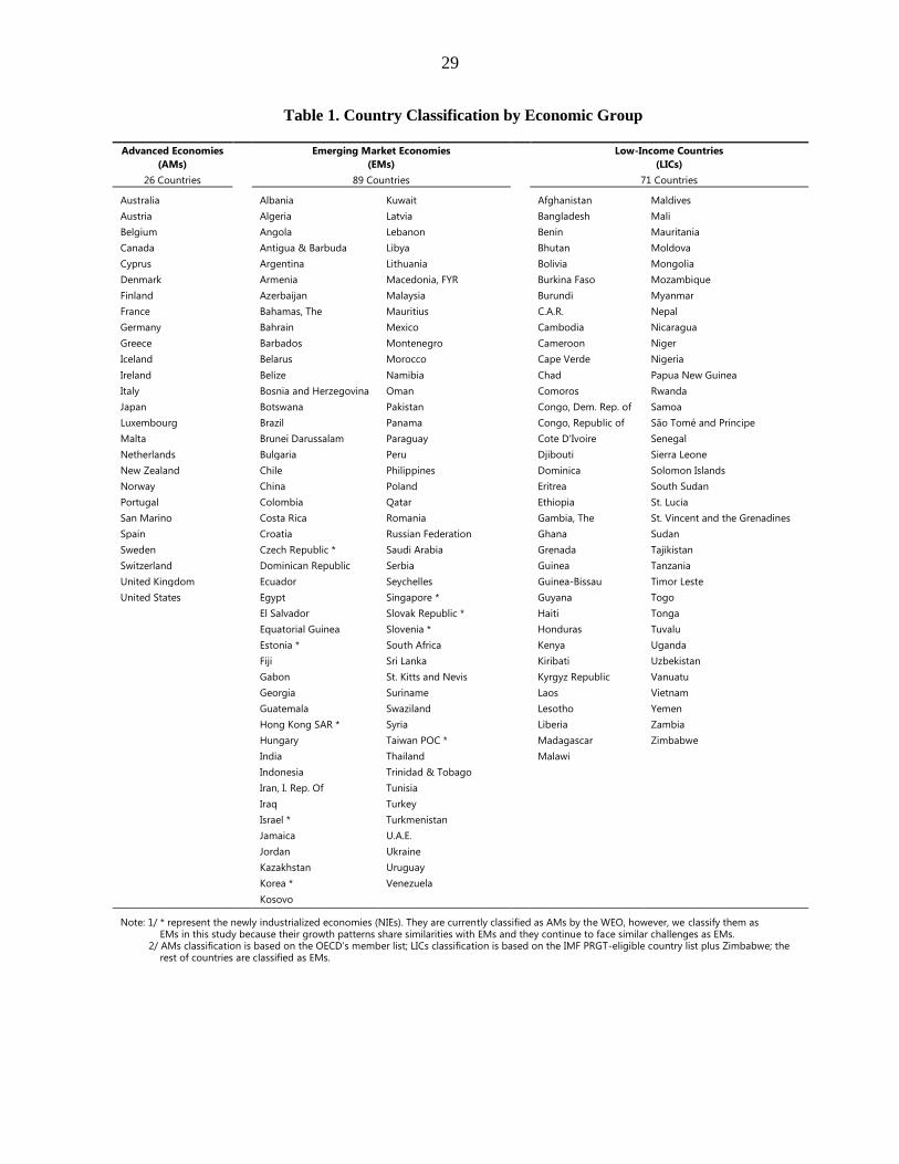
29

Table 1. Country Classification by Economic Group

Advanced Economies

(AMs)

Emerging Market Economies

(EMs)

Low-Income Countries

(LICs)

26 Countries

89 Countries

71 Countries

Australia

Albania Kuwait

Afghanistan Maldives

Austria

Algeria Latvia

Bangladesh Mali

Belgium

Angola Lebanon

Benin Mauritania

Canada

Antigua & Barbuda Libya

Bhutan Moldova

Cyprus

Argentina Lithuania

Bolivia Mongolia

Denmark

Armenia Macedonia, FYR

Burkina Faso Mozambique

Finland

Azerbaijan Malaysia

Burundi Myanmar

France

Bahamas, The Mauritius

C.A.R. Nepal

Germany

Bahrain Mexico

Cambodia Nicaragua

Greece

Barbados Montenegro

Cameroon Niger

Iceland

Belarus Morocco

Cape Verde Nigeria

Ireland

Belize Namibia

Chad Papua New Guinea

Italy

Bosnia and Herzegovina Oman

Comoros Rwanda

Japan

Botswana Pakistan

Congo, Dem. Rep. of Samoa

Luxembourg

Brazil Panama

Congo, Republic of São Tomé and Príncipe

Malta

Brunei Darussalam Paraguay

Cote D'Ivoire Senegal

Netherlands

Bulgaria Peru

Djibouti Sierra Leone

New Zealand

Chile Philippines

Dominica Solomon Islands

Norway

China Poland

Eritrea South Sudan

Portugal

Colombia Qatar

Ethiopia St. Lucia

San Marino

Costa Rica Romania

Gambia, The St. Vincent and the Grenadines

Spain

Croatia Russian Federation

Ghana Sudan

Sweden

Czech Republic * Saudi Arabia

Grenada Tajikistan

Switzerland

Dominican Republic Serbia

Guinea Tanzania

United Kingdom

Ecuador Seychelles

Guinea-Bissau Timor Leste

United States

Egypt Singapore *

Guyana Togo

El Salvador Slovak Republic *

Haiti Tonga

Equatorial Guinea Slovenia *

Honduras Tuvalu

Estonia * South Africa

Kenya Uganda

Fiji Sri Lanka

Kiribati Uzbekistan

Gabon St. Kitts and Nevis

Kyrgyz Republic Vanuatu

Georgia Suriname

Laos Vietnam

Guatemala Swaziland

Lesotho Yemen

Hong Kong SAR * Syria

Liberia Zambia

Hungary Taiwan POC * Madagascar Zimbabwe

India Thailand

Malawi

Indonesia Trinidad & Tobago

Iran, I. Rep. Of Tunisia

Iraq Turkey

Israel * Turkmenistan

Jamaica U.A.E.

Jordan Ukraine

Kazakhstan Uruguay

Korea * Venezuela

Kosovo

Note: 1/ * represent the newly industrialized economies (NIEs). They are currently classified as AMs by the WEO, however, we classify them as EMs in this study because their growth patterns share similarities with EMs and they continue to face similar challenges as EMs. 2/ AMs classification is based on the OECD’s member list; LICs classification is based on the IMF PRGT-eligible country list plus Zimbabwe; the rest of countries are classified as EMs.

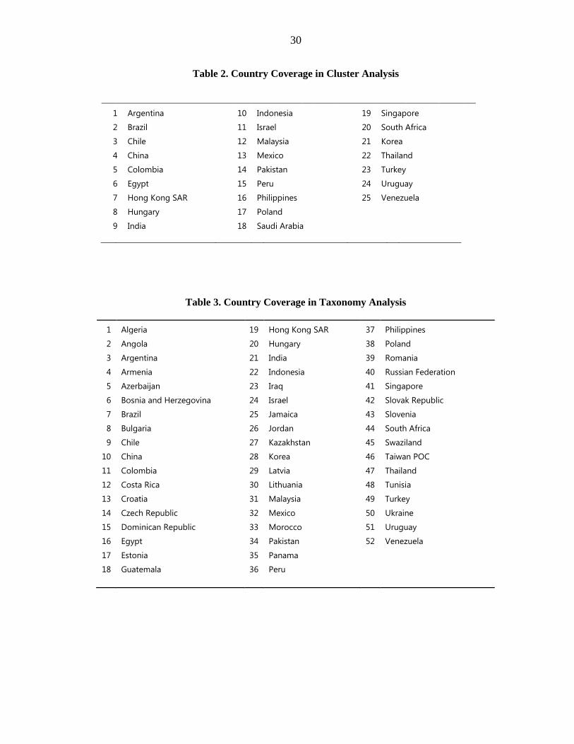
30

Table 2. Country Coverage in Cluster Analysis

1 Argentina 10 Indonesia 19 Singapore

2 Brazil 11 Israel 20 South Africa

3 Chile 12 Malaysia 21 Korea

4 China 13 Mexico 22 Thailand

5 Colombia 14 Pakistan 23 Turkey

6 Egypt 15 Peru 24 Uruguay

7 Hong Kong SAR 16 Philippines 25 Venezuela

8 Hungary 17 Poland

9 India 18 Saudi Arabia

Table 3. Country Coverage in Taxonomy Analysis

1 Algeria 19 Hong Kong SAR 37 Philippines

2 Angola 20 Hungary 38 Poland

3 Argentina 21 India 39 Romania

4 Armenia 22 Indonesia 40 Russian Federation

5 Azerbaijan 23 Iraq 41 Singapore

6 Bosnia and Herzegovina 24 Israel 42 Slovak Republic

7 Brazil 25 Jamaica 43 Slovenia

8 Bulgaria 26 Jordan 44 South Africa

9 Chile 27 Kazakhstan 45 Swaziland

10 China 28 Korea 46 Taiwan POC

11 Colombia 29 Latvia 47 Thailand

12 Costa Rica 30 Lithuania 48 Tunisia

13 Croatia 31 Malaysia 49 Turkey

14 Czech Republic 32 Mexico 50 Ukraine

15 Dominican Republic 33 Morocco 51 Uruguay

16 Egypt 34 Pakistan 52 Venezuela

17 Estonia 35 Panama

18 Guatemala 36 Peru

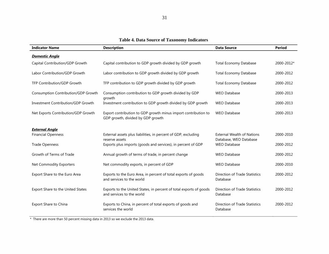
31

Table 4. Data Source of Taxonomy Indicators

Indicator Name Description Data Source Period

Domestic Angle

Capital Contribution/GDP Growth

Capital contribution to GDP growth divided by GDP growth Total Economy Database 2000-2012*

Labor Contribution/GDP Growth

Labor contribution to GDP growth divided by GDP growth Total Economy Database 2000-2012

TFP Contribution/GDP Growth

TFP contribution to GDP growth divided by GDP growth Total Economy Database 2000-2012

Consumption Contribution/GDP Growth

Consumption contribution to GDP growth divided by GDP

growth

WEO Database 2000-2013

Investment Contribution/GDP Growth

Investment contribution to GDP growth divided by GDP growth WEO Database 2000-2013

Net Exports Contribution/GDP Growth Export contribution to GDP growth minus import contribution to

GDP growth, divided by GDP growth

WEO Database 2000-2013

External Angle

Financial Openness External assets plus liabilities, in percent of GDP, excluding

reserve assets

External Wealth of Nations

Database, WEO Database

2000-2010

Trade Openness

Exports plus imports (goods and services), in percent of GDP WEO Database 2000-2012

Growth of Terms of Trade

Annual growth of terms of trade, in percent change WEO Database 2000-2012

Net Commodity Exporters

Net commodity exports, in percent of GDP WEO Database 2000-2010

Export Share to the Euro Area Exports to the Euro Area, in percent of total exports of goods

and services to the world

Direction of Trade Statistics

Database

2000-2012

Export Share to the United States

Exports to the United States, in percent of total exports of goods

and services to the world

Direction of Trade Statistics

Database

2000-2012

Export Share to China Exports to China, in percent of total exports of goods and

services the world

Direction of Trade Statistics

Database

2000-2012

* There are more than 50 percent missing data in 2013 so we exclude the 2013 data.

32

REFERENCE

Agénor, PR., O. Canuto, and M. Jelenic, 2012. "Avoiding Middle-Income Growth Traps," World

Bank - Economic Premise, issue 98 (November), pp. 1-7. (Washington: World Bank).

Blanchard, O.J. and P.A. Diamond, 1989, "The Beveridge Curve," Brookings Papers on Economic

Activity, Vol. 1, pp. 1-60.

Cubeddu, L., A. Culiuc, G. Fayad, Y. Gao, K. Kochhar, A. Kyobe, C. Oner, R. Perrelli, S. Sanya, E.

Tsounta, and Z. Zhang, 2014, “Emerging Markets in Transition: Growth Prospects and

Challenges,” Staff Discussion Note 14/6 (Washington: International Monetary Fund).

Fayad, G. and R. Perrelli, 2014, “Growth Surprises and Synchronized Slowdowns in Emerging

Markets––An Empirical Investigation,” IMF Working paper WP/14/173 (Washington:

International Monetary Fund).

Gourinchas Pierre-Olivier. and Rey, Helene, 2013, “External Adjustment, Global Imbalances, and

Valuation Effects,” NBER Working Paper No. 19240.

International Monetary Fund, 2014, “World Economic Outlook—Recovery Strengthens, Remains

Uneven,” (Washington, April 2014).

Mishra, P., K. Moriyama, P. N’Diaye, and L. Nguyen, 2014, “Impact of Fed Tapering

Announcements on Emerging Markets Affected? ” IMF Working paper WP/14/109

(Washington: International Monetary Fund).

Lane, P.R. and G.M. Milesi-Ferretti, 2007, "The External Wealth of Nations Mark II: Revised and

Extended Estimates of Foreign Assets and Liabilities, 1970–2004," Journal of International

Economics 73(November), pp. 223-250.

Lequiller, F. and D. Blades, 2006, “Understanding National Accounts,” (Paris: OECD).

Lipton, D., 2013, “Emerging Markets in Transition,” Presented at the IMF/World Bank Annual

Meetings Conference on October 8, 2013.

Rey, Helene, 2013, “Dilemma not Trilemma: The Global Financial Cycle and Monetary Policy

Independence,” Jackson Hole Conference Proceedings, Kansas City Fed..

Rostow, W. W., 1959, “The Stages of Economic Growth,” The Economic History Review, Volume

12, Issue 1, pages 1–16.

Sala-I-Martin, Xavier X., 1997, "I Just Ran Two Million Regressions," The American Economic

Review, Vol. 87, No. 2, Papers and Proceedings of the Hundred and Fourth Annual Meeting

of the American Economic Association, pp. 178-183.

33

Solow, R., 1956, "A Contribution to the Theory of Economic Growth," The Quarterly Journal of

Economics, Vol. 70, No. 1, pp. 65-94.

StataCorp, 2013, “Stata 13 Base Reference Manual—Introduction to cluster-analysis commands,”

College Station, TX: Stata Press.

The Conference Board, 2014, “Total Economy Database Methodological Notes,” (New York: The

Conference Board).

Vázqueza, S.T. and A. Sumner, 2013, "Revisiting the Meaning of Development: A Multidimensional

Taxonomy of Developing Countries," The Journal of Development Studies, Vol. 49, issue

12, pp. 1728-1745.