1

Emergency Communications during the Minneapolis Bridge Disaster:

A Technical Case Study by the Federal Communications Commission’s

Public Safety and Homeland Security Bureau’s Communications Systems Analysis Division

November 13, 2008

2

Table of Contents

1. Executive Summary .................................................................................................... 5 2. Introduction................................................................................................................. 7 3. Minneapolis Bridge Disaster....................................................................................... 9 4. Overview of Minneapolis LMR System................................................................... 13 5. Characterization of Public Safety Communications Traffic During the Disaster..... 16 6. Performance Modeling and Evaluation of Trunked LMR Systems.......................... 23

6.1. Choosing the Site with Highest System Utilization.......................................... 23 6.2. Systems Modeling............................................................................................. 24

6.2.1. System Performance ................................................................................. 25 6.2.2. Talkgroup Performance ............................................................................ 26

6.3. Analysis and Discussion of Minneapolis LMR System ................................... 26 6.3.1. Data Collection ......................................................................................... 26 Past System Performance and Calibration of Model ................................................ 26

6.4. Performance Analysis of Trunked LMR Systems ............................................ 29 6.5. Capacity Analysis of Trunked LMR Systems .................................................. 31 6.6. An Analysis on Talkgroup Performance........................................................... 34

6.6.1. Background............................................................................................... 34 6.6.2. Analysis..................................................................................................... 35

7. Potential Applications of Commercial Wireless Broadband Technologies.............. 41 7.1. Approach........................................................................................................... 41 7.2. Modeling the 4G Broadband WiMAX network ............................................... 42 7.3. Voice Analysis .................................................................................................. 44 7.4. Voice and Video Analysis ................................................................................ 46

8. Conclusions............................................................................................................... 48 9. Appendix A: LMR Performance Modeling & Analysis ........................................... 49

9.1. Systems Modeling............................................................................................. 49 9.1.1. Modeling Approach .................................................................................. 49 9.1.2. System Parameters and Performance Metrics........................................... 51

9.2. Prior Work for LMR Performance Analysis by Others .................................... 55 10. Appendix B: Baseline calculation of Voice over IP (VoIP) ................................ 58

3

Table of Figures Figure 1 – Minneapolis Bridge After Collapse................................................................... 9 Figure 2 – Minneapolis Bridge After Collapse................................................................... 9 Figure 3 – Navy Divers At the Scene ............................................................................... 11 Figure 4 – A Simulcast Group .......................................................................................... 14 Figure 5 – Roaming Among Simulcast Groups................................................................ 14 Figure 6 – Push to Talks – August 1, 2007 vs. Historical ................................................ 16 Figure 7 – Travel in Excess of Typical Peak Hour – August 1, 2007 .............................. 17 Figure 8 – Call Air Time by Occurrence – August 1, 2007.............................................. 18 Figure 9 - Call Air Time Cumulative Distribution – August 1, 2007............................... 18 Figure 10 - Total Air Seconds per Caller – August 1, 2007 ............................................. 20 Figure 11 – Cumulative Air Time per Caller – August 1, 2007 ....................................... 20 Figure 12 – Queue Time – August 1, 2007....................................................................... 21 Figure 13 – System Utilization for all Sites...................................................................... 23 Figure 14 – Cell 1 Call Requests ...................................................................................... 24 Figure 15 – Waiting Time vs. System Utilization ............................................................ 30 Figure 16 - Percentage of Calls Waiting More Than 3 Seconds vs. System Utilization .. 30 Figure 17 – Capacity Region ............................................................................................ 32 Figure 18 – Operational Region........................................................................................ 32 Figure 19 – Capacity Region ............................................................................................ 33 Figure 20 - Operational Region ........................................................................................ 34 Figure 21 - Air Seconds .................................................................................................... 36 Figure 22 - Top 20 Talk Group Usage for Site 1.............................................................. 36 Figure 23– Locally perceived User Waiting Time vs. Talkgroup Utilization .................. 37 Figure 24 – Locally Perceived User waiting Time vs. Talkgroup Utilization.................. 38 Figure 25 - WiMAX Network Diagram............................................................................ 44 Figure 26 - End to End System Model for a Trunked LMR System ................................ 49 Figure 27 – Queue Models................................................................................................ 50 Figure 28 ........................................................................................................................... 53

4

List of Tables Table 1 - System Performance for Busiest Site (N=20 voice channels) - Modeled vs. Actual................................................................................................................................ 28 Table 2 - System Performance of a Site with 20 Voice Channels and Call Duration of 5.927 sec ........................................................................................................................... 29 Table 3 - Capacity for GoS of WC =1 sec versus Offered Load and Utilization (Call Dur 5.927 sec) .......................................................................................................................... 31 Table 4 - Capacity for GOS of “2% of calls waiting more than 3 secs” versus offered load or utilization, with call duration of 1/µ=5.927 sec............................................................ 33 Table 5 – Top 20 Talkgroups for Site 1............................................................................ 36 Table 6 - System Utilization vs. Waiting Time in Central Queue .................................... 38 Table 7 – Talkgroup Utilization Threshold vs. System Utilization .................................. 40 Table 8 - WIMAX Parameters.......................................................................................... 43 Table 9 - Summary with No Commercial Traffic............................................................. 45 Table 10 - Detailed Summary Results .............................................................................. 46 Table 11 - Results for Voice and Video Analysis............................................................. 47 Table 12 - System performance for busiest site (N=20 voice channels) for 3 different times using Gamma/Lognormal distributions................................................................... 56 Table 13 - System performance for busiest site (N=20 voice channels) for 3 different times using exponential/exponential distributions............................................................ 57

5

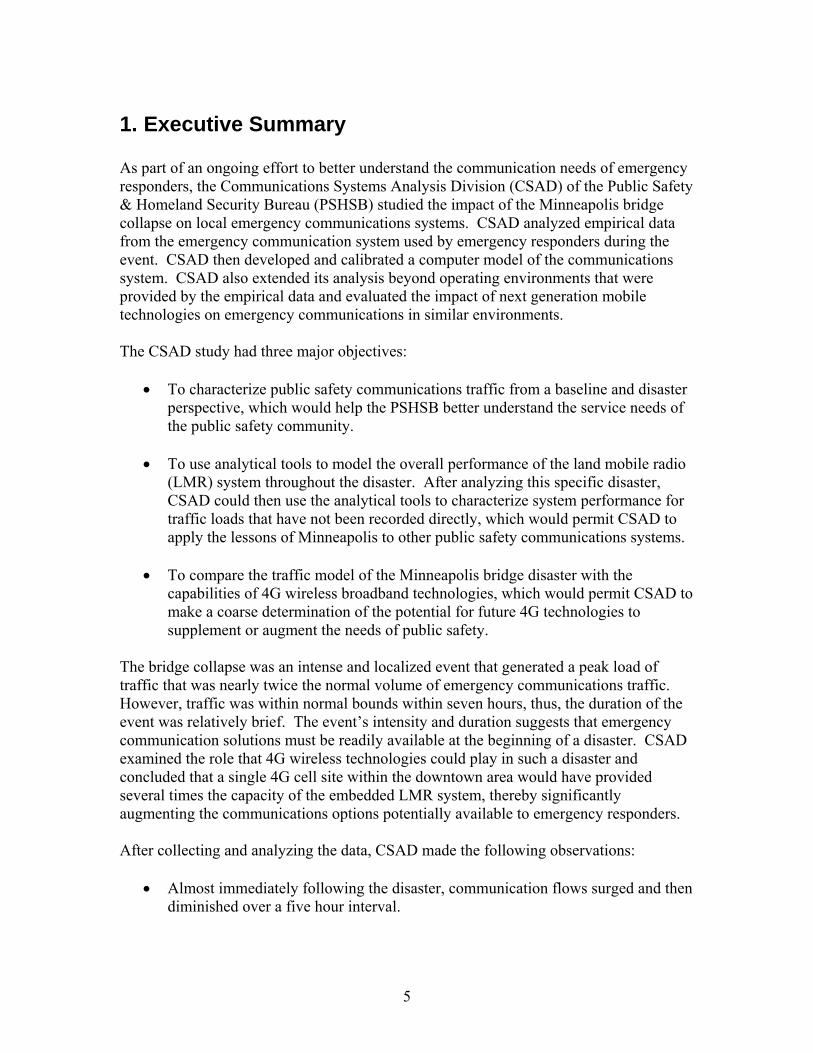
1. Executive Summary As part of an ongoing effort to better understand the communication needs of emergency responders, the Communications Systems Analysis Division (CSAD) of the Public Safety & Homeland Security Bureau (PSHSB) studied the impact of the Minneapolis bridge collapse on local emergency communications systems. CSAD analyzed empirical data from the emergency communication system used by emergency responders during the event. CSAD then developed and calibrated a computer model of the communications system. CSAD also extended its analysis beyond operating environments that were provided by the empirical data and evaluated the impact of next generation mobile technologies on emergency communications in similar environments. The CSAD study had three major objectives:

• To characterize public safety communications traffic from a baseline and disaster perspective, which would help the PSHSB better understand the service needs of the public safety community.

• To use analytical tools to model the overall performance of the land mobile radio

(LMR) system throughout the disaster. After analyzing this specific disaster, CSAD could then use the analytical tools to characterize system performance for traffic loads that have not been recorded directly, which would permit CSAD to apply the lessons of Minneapolis to other public safety communications systems.

• To compare the traffic model of the Minneapolis bridge disaster with the

capabilities of 4G wireless broadband technologies, which would permit CSAD to make a coarse determination of the potential for future 4G technologies to supplement or augment the needs of public safety.

The bridge collapse was an intense and localized event that generated a peak load of traffic that was nearly twice the normal volume of emergency communications traffic. However, traffic was within normal bounds within seven hours, thus, the duration of the event was relatively brief. The event’s intensity and duration suggests that emergency communication solutions must be readily available at the beginning of a disaster. CSAD examined the role that 4G wireless technologies could play in such a disaster and concluded that a single 4G cell site within the downtown area would have provided several times the capacity of the embedded LMR system, thereby significantly augmenting the communications options potentially available to emergency responders. After collecting and analyzing the data, CSAD made the following observations:

• Almost immediately following the disaster, communication flows surged and then diminished over a five hour interval.

6

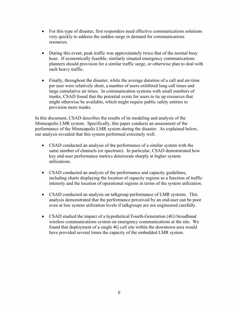
• For this type of disaster, first responders need effective communications solutions very quickly to address the sudden surge in demand for communications resources.

• During this event, peak traffic was approximately twice that of the normal busy

hour. If economically feasible, similarly situated emergency communications planners should provision for a similar traffic surge, or otherwise plan to deal with such heavy traffic.

• Finally, throughout the disaster, while the average duration of a call and air-time

per user were relatively short, a number of users exhibited long call times and large cumulative air times. In communication systems with small numbers of trunks, CSAD found that the potential exists for users to tie up resources that might otherwise be available, which might require public safety entities to provision more trunks.

In this document, CSAD describes the results of its modeling and analysis of the Minneapolis LMR system. Specifically, this paper conducts an assessment of the performance of the Minneapolis LMR system during the disaster. As explained below, our analysis revealed that this system performed extremely well.

• CSAD conducted an analysis of the performance of a similar system with the same number of channels (or spectrum). In particular, CSAD demonstrated how key end-user performance metrics deteriorate sharply at higher system utilizations.

• CSAD conducted an analysis of the performance and capacity guidelines,

including charts displaying the location of capacity regions as a function of traffic intensity and the location of operational regions in terms of the system utilization.

• CSAD conducted an analysis on talkgroup performance of LMR systems. This

analysis demonstrated that the performance perceived by an end-user can be poor even at low system utilization levels if talkgroups are not engineered carefully.

• CSAD studied the impact of a hypothetical Fourth-Generation (4G) broadband

wireless communications system on emergency communications at the site. We found that deployment of a single 4G cell site within the downtown area would have provided several times the capacity of the embedded LMR system.

7

2. Introduction As part of an ongoing effort to better understand the communication needs of emergency responders, CSAD studied the impact of the Minneapolis bridge collapse on local emergency communications systems. CSAD would like to ensure that the public safety community is informed about the evolution of communication capabilities and services. The PSHSB recently completed a congressionally-mandated study of public safety communications systems and these systems’ potential backup capabilities.1 During this study, public safety leaders provided valuable information about their communication needs and explained the mission critical role that public safety communication systems must perform. The study revealed that public safety communication systems’ technical requirements and usage differ from their commercial counterparts. More recently, CSAD examined the potential applicability of emerging technologies on the public safety communication sector. Major wireless service providers2 have recently announced that they would be deploying wireless broadband technology (commonly called 4G wireless) across the nation. In addition, the FCC recently sought comment on a tentative conclusion to require, as a license condition, that the 700 MHz D Block licensee enter into a public/private partnership for the purpose of constructing a broadband network that will operate over both D block spectrum and public safety broadband spectrum and provide broadband services to both commercial users and public safety entities.3 Further, by augmenting carriers’ emergency communication services via the Wireless Priority Service (WPS) program, the Department of Homeland Security (DHS) is enhancing the potential for future commercial service provider networks to offer advanced services.4 In order to develop mechanisms to better characterize public safety system’s performance in stress situations, CSAD studied the performance characteristics of current generation public safety wireless voice communication systems. As part of this study, CSAD examined the network performance of an LMR system during a crisis in a major metropolitan area, the Minneapolis bridge disaster. The bridge collapse was a major disaster requiring a complex response from multiple agencies. As a result, the disaster was well documented by government agencies, such as the Federal Emergency

1 See FCC Report to Congress: Vulnerability Assessment and Feasibility of Creating a Backup Emergency Communication System, available at http://www.fcc.gov/pshs/clearinghouse/case-studies.html (Jan. 30, 2008)(Vulnerability Assessment). 2 See Lynnette Luna, “Verizon, AT&T Both Plan 2010 Launch for LTE Networks, MRT Magazine, (May 1, 2007), available at http://mrtmag.com/networks_and_systems/mag/radio_verizon_att_plan/ (last visited 6/23/2008); See also Elizabeth Woyke, “Betting Billions”, Forbes.com, (Oct. 7, 2008). 3 See Service Rules for the 698-746, 747-762 and 777-792 MHz Bands, Implementing a Nationwide, Broadband, Interoperable Public Safety Network in the 700 MHz Band, WT Docket No. 06-150, PS Docket No. 06-229, Third Further Notice of Proposed Rulemaking, FCC 08-230 (Rel. Sept. 25 2008). 4 The Department of Homeland Security/National Communication System is working with industry groups to extend the National Security/Emergency Preparedness (NS/EP) Priority Telecommunication Service WPS to both WiMax and LTE and IP Multimedia Service (IMS), the control architecture defined for future wireless broadband networks.

8

Management Agency (FEMA)5 and the Homeland Security/Office of Emergency Communications (OEC).6 Moreover, the recent nature of the disaster suggested that CSAD would have readily available network data. Minneapolis public safety agencies had recently transitioned to a shared LMR system. This system performed flawlessly throughout the disaster. Because the system was able to handle the high traffic loads, CSAD believed that a complete traffic profile was likely to be available, which was confirmed by the Minneapolis public safety officials. CSAD would like to gratefully acknowledge the cooperation of Roger Laurence, Radio Communications Manager, Hennepin County, Alan Fjerstad, 800 MHz Radio Systems Administrator, Hennepin County Sheriff’s Office, King Fung (Senior Professional Engineer) and John Gundersen (Assistant Communications Manager) who provided access to the data used in this report and shared their knowledge of LMR system operation and performance. Their generosity in this regard was exceptional and made this report possible.

5Dep’t of Homeland Security, FEMA, U.S. Fire Administration/Technical Report Series, I-35 Bridge Collapse and Response, USFA-TR-166 (Aug. 2007). 6 Dep’t of Homeland Security, Office of Emergency Communications Bulletin, Successful Communications at Minnesota Bridge Collapse (October/November 2007)(FEMA Report).

9

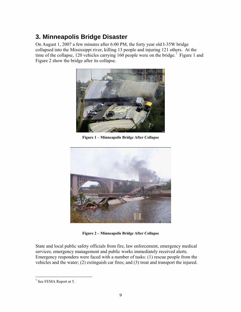
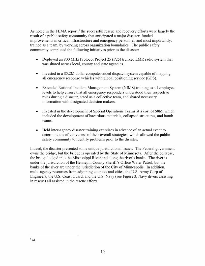
3. Minneapolis Bridge Disaster On August 1, 2007 a few minutes after 6:00 PM, the forty year old I-35W bridge collapsed into the Mississippi river, killing 13 people and injuring 121 others. At the time of the collapse, 120 vehicles carrying 160 people were on the bridge.7 Figure 1 and Figure 2 show the bridge after its collapse.

Figure 1 – Minneapolis Bridge After Collapse

Figure 2 – Minneapolis Bridge After Collapse

State and local public safety officials from fire, law enforcement, emergency medical services, emergency management and public works immediately received alerts. Emergency responders were faced with a number of tasks: (1) rescue people from the vehicles and the water; (2) extinguish car fires; and (3) treat and transport the injured.

7 See FEMA Report at 5.

10

As noted in the FEMA report,8 the successful rescue and recovery efforts were largely the result of a public safety community that anticipated a major disaster, funded improvements in critical infrastructure and emergency personnel, and most importantly, trained as a team, by working across organization boundaries. The public safety community completed the following initiatives prior to the disaster:

• Deployed an 800 MHz Protocol Project 25 (P25) trunked LMR radio system that was shared across local, county and state agencies.

• Invested in a $5.2M dollar computer-aided dispatch system capable of mapping

all emergency response vehicles with global positioning service (GPS).

• Extended National Incident Management System (NIMS) training to all employee levels to help ensure that all emergency responders understood their respective roles during a disaster, acted as a collective team, and shared necessary information with designated decision makers.

• Invested in the development of Special Operations Teams at a cost of $8M, which

included the development of hazardous materials, collapsed structures, and bomb teams.

• Held inter-agency disaster training exercises in advance of an actual event to

determine the effectiveness of their overall strategies, which allowed the public safety community to identify problems prior to the disaster.

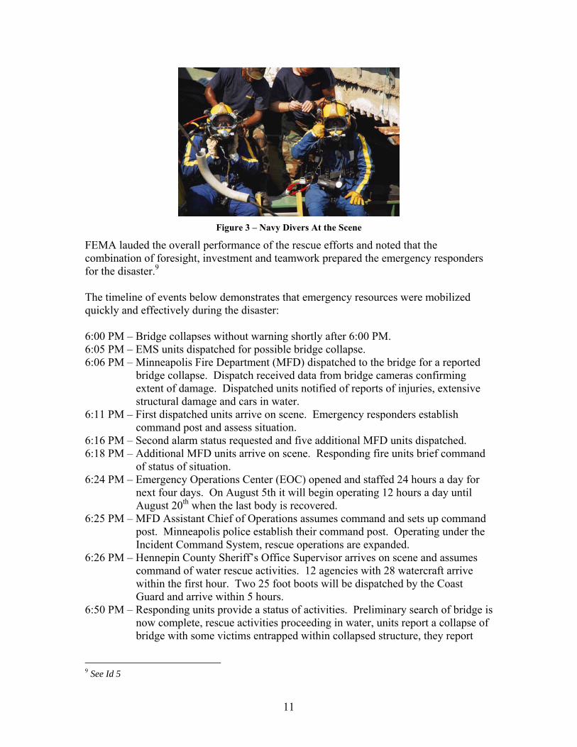
Indeed, the disaster presented some unique jurisdictional issues. The Federal government owns the bridge, but the bridge is operated by the State of Minnesota. After the collapse, the bridge lodged into the Mississippi River and along the river’s banks. The river is under the jurisdiction of the Hennepin County Sheriff’s Office Water Patrol, but the banks of the river are under the jurisdiction of the City of Minneapolis. In addition, multi-agency resources from adjoining counties and cities, the U.S. Army Corp of Engineers, the U.S. Coast Guard, and the U.S. Navy (see Figure 3, Navy divers assisting in rescue) all assisted in the rescue efforts.

8 Id.

11

Figure 3 – Navy Divers At the Scene

FEMA lauded the overall performance of the rescue efforts and noted that the combination of foresight, investment and teamwork prepared the emergency responders for the disaster.9 The timeline of events below demonstrates that emergency resources were mobilized quickly and effectively during the disaster: 6:00 PM – Bridge collapses without warning shortly after 6:00 PM. 6:05 PM – EMS units dispatched for possible bridge collapse. 6:06 PM – Minneapolis Fire Department (MFD) dispatched to the bridge for a reported

bridge collapse. Dispatch received data from bridge cameras confirming extent of damage. Dispatched units notified of reports of injuries, extensive structural damage and cars in water.

6:11 PM – First dispatched units arrive on scene. Emergency responders establish command post and assess situation.

6:16 PM – Second alarm status requested and five additional MFD units dispatched. 6:18 PM – Additional MFD units arrive on scene. Responding fire units brief command

of status of situation. 6:24 PM – Emergency Operations Center (EOC) opened and staffed 24 hours a day for

next four days. On August 5th it will begin operating 12 hours a day until August 20th when the last body is recovered.

6:25 PM – MFD Assistant Chief of Operations assumes command and sets up command post. Minneapolis police establish their command post. Operating under the Incident Command System, rescue operations are expanded.

6:26 PM – Hennepin County Sheriff’s Office Supervisor arrives on scene and assumes command of water rescue activities. 12 agencies with 28 watercraft arrive within the first hour. Two 25 foot boots will be dispatched by the Coast Guard and arrive within 5 hours.

6:50 PM – Responding units provide a status of activities. Preliminary search of bridge is now complete, rescue activities proceeding in water, units report a collapse of bridge with some victims entrapped within collapsed structure, they report

9 See Id 5

12

fires are being contained, and that an engineer is on the bridge to assess its stability.

7:00 PM – Engineers report that bridge stability is questionable. 7:27 PM – It is determined that all individuals on the bridge and next to the water have

been rescued. Rescue phase of operation is now complete. Recovery operations will officially begin at dawn on 8/2, the following day.

7:55 PM – Last live rescue victim transported from scene. 8:11 PM – 50 patients have now been transported to various hospitals by EMS. 61 units

including 31 ambulances have responded. 110 people will require treatment at hospitals or emergency clinics. 13 deaths will be reported.

Until midnight on August 2nd, the 911 call center received approximately 300 calls per hour. The public safety community conducted recovery operations until August 20th and operations associated with the removal of debris, monitoring of hazardous material, and other activities associated with the disaster continued for even more time.

13

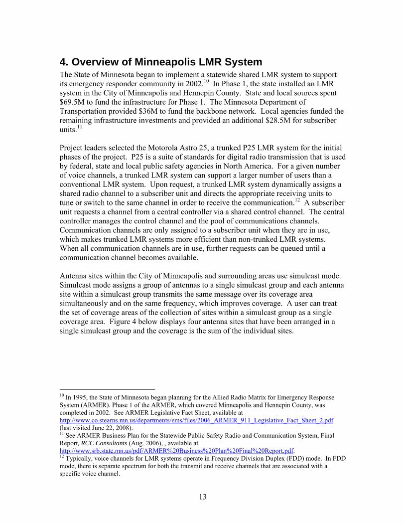
4. Overview of Minneapolis LMR System The State of Minnesota began to implement a statewide shared LMR system to support its emergency responder community in 2002.10 In Phase 1, the state installed an LMR system in the City of Minneapolis and Hennepin County. State and local sources spent $69.5M to fund the infrastructure for Phase 1. The Minnesota Department of Transportation provided $36M to fund the backbone network. Local agencies funded the remaining infrastructure investments and provided an additional $28.5M for subscriber units.11 Project leaders selected the Motorola Astro 25, a trunked P25 LMR system for the initial phases of the project. P25 is a suite of standards for digital radio transmission that is used by federal, state and local public safety agencies in North America. For a given number of voice channels, a trunked LMR system can support a larger number of users than a conventional LMR system. Upon request, a trunked LMR system dynamically assigns a shared radio channel to a subscriber unit and directs the appropriate receiving units to tune or switch to the same channel in order to receive the communication.12 A subscriber unit requests a channel from a central controller via a shared control channel. The central controller manages the control channel and the pool of communications channels. Communication channels are only assigned to a subscriber unit when they are in use, which makes trunked LMR systems more efficient than non-trunked LMR systems. When all communication channels are in use, further requests can be queued until a communication channel becomes available. Antenna sites within the City of Minneapolis and surrounding areas use simulcast mode. Simulcast mode assigns a group of antennas to a single simulcast group and each antenna site within a simulcast group transmits the same message over its coverage area simultaneously and on the same frequency, which improves coverage. A user can treat the set of coverage areas of the collection of sites within a simulcast group as a single coverage area. Figure 4 below displays four antenna sites that have been arranged in a single simulcast group and the coverage is the sum of the individual sites.

10 In 1995, the State of Minnesota began planning for the Allied Radio Matrix for Emergency Response System (ARMER). Phase 1 of the ARMER, which covered Minneapolis and Hennepin County, was completed in 2002. See ARMER Legislative Fact Sheet, available at http://www.co.stearns.mn.us/departments/ems/files/2006_ARMER_911_Legislative_Fact_Sheet_2.pdf (last visited June 22, 2008). 11 See ARMER Business Plan for the Statewide Public Safety Radio and Communication System, Final Report, RCC Consultants (Aug. 2006), , available at http://www.srb.state.mn.us/pdf/ARMER%20Business%20Plan%20Final%20Report.pdf. 12 Typically, voice channels for LMR systems operate in Frequency Division Duplex (FDD) mode. In FDD mode, there is separate spectrum for both the transmit and receive channels that are associated with a specific voice channel.

14

Figure 4 – A Simulcast Group

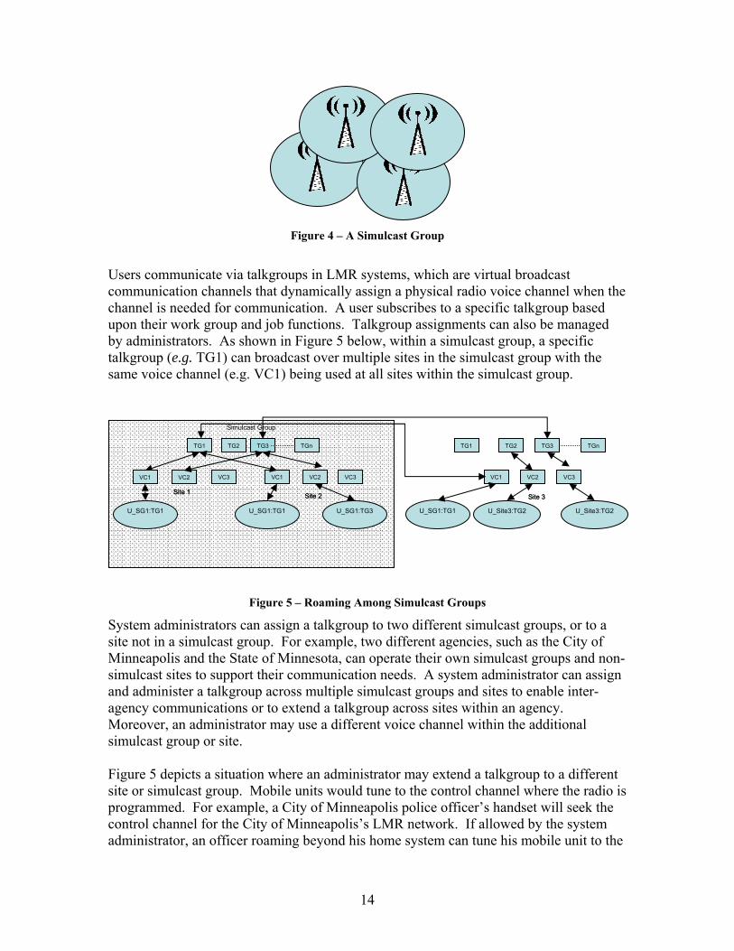
Users communicate via talkgroups in LMR systems, which are virtual broadcast communication channels that dynamically assign a physical radio voice channel when the channel is needed for communication. A user subscribes to a specific talkgroup based upon their work group and job functions. Talkgroup assignments can also be managed by administrators. As shown in Figure 5 below, within a simulcast group, a specific talkgroup (e.g. TG1) can broadcast over multiple sites in the simulcast group with the same voice channel (e.g. VC1) being used at all sites within the simulcast group.

Figure 5 – Roaming Among Simulcast Groups

System administrators can assign a talkgroup to two different simulcast groups, or to a site not in a simulcast group. For example, two different agencies, such as the City of Minneapolis and the State of Minnesota, can operate their own simulcast groups and non-simulcast sites to support their communication needs. A system administrator can assign and administer a talkgroup across multiple simulcast groups and sites to enable inter-agency communications or to extend a talkgroup across sites within an agency. Moreover, an administrator may use a different voice channel within the additional simulcast group or site. Figure 5 depicts a situation where an administrator may extend a talkgroup to a different site or simulcast group. Mobile units would tune to the control channel where the radio is programmed. For example, a City of Minneapolis police officer’s handset will seek the control channel for the City of Minneapolis’s LMR network. If allowed by the system administrator, an officer roaming beyond his home system can tune his mobile unit to the

Simulcast Group

TG1 TG2 TG3 TGn TG2 TG3 TGn

VC2 VC3 VC1 VC2 VC1 VC3

Site 1 Site 2 Site 3

U_SG1:TG1 U_SG1:TG3 U_SG1:TG1 U_Site3:TG2 U_Site3:TG2

TG1

VC1 VC3 VC2

Site 1 Site 2 Site 3

U_SG1:TG1

VC1

15

control channel of the local LMR site where the officer has roamed. This process of roaming support is called affiliation. When a subscriber’s mobile unit affiliates with a local LMR site, communications over the talkgroups where the handset is subscribed will be repeated over the local LMR site, as long as the mobile unit remains affiliated with the site. In effect, the talkgroup extends to the site when the Minneapolis police officer becomes affiliated with the site. In Figure 5, a user of Simulcast Group 1 (U_SG1) roamed to Site 3 and affiliated with the site. Thus, messages on Talkgroup 1, where the unit is assigned, will be broadcast over Site 3 and will continue as long as the user remains affiliated with the site. Simulcasting and affiliation’s flexibility come with tradeoffs. Since a single message is broadcast over multiple sites, simulcast groups reduce system capacity because talkgroups span multiple sites. Groups increase the system load because each message is rebroadcast over multiple simulcast groups and sites. Affiliated mobile units cause foreign traffic to be broadcast over the local site, as long as the affiliated mobile unit remains within the coverage area of the site. These latter two mechanisms, in effect, multiply the traffic at a local site due to the foreign traffic being injected into the local network. During the evening of the disaster, traffic analysis indicated that a portion of the messages were rebroadcast to possibly eight other foreign simulcast groups or sites. Our traffic analysis also found that, on average, a message would be broadcast to one or two other groups or sites.

16

5. Characterization of Public Safety Communications Traffic During the Disaster

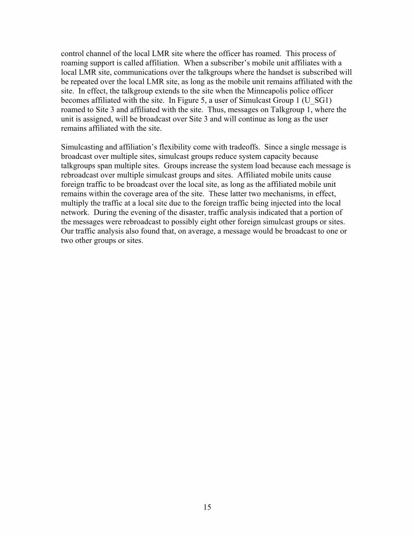
Although activities associated with this disaster continued for many days, the emergency communications system was under a heavy load for a comparatively short period of time. Figure 6 below displays the number of Push to Talks (PTTs) 13 at 15 minute intervals on the shared radio system during the event. Figure 6 also displays a comparable period from about a week prior to the event.

Push to Talks (PTT)Bridge Collapse 8/1/07

0

500

1000

1500

2000

2500

3000

3500

4000

4500

16:00

17:00

18:00

19:00

20:00

21:00

22:00

23:00

0:00

1:00

2:00

3:00

4:00

5:00

6:00

Time

Num

ber

of P

TTs

PTTs 8/1/07Bridge CollapsePTTs 7/26/07

Figure 6 – Push to Talks – August 1, 2007 vs. Historical

On August 1, 2007, at 5:00 PM, voice traffic sharply rose towards a busy period. Shortly after 6:00 PM, there was a sharp spike in voice traffic, which rose steadily until a peak at 7:30 PM. Voice traffic then began to sharply decline shortly after 8:00 PM, which corresponds with our timeline, as rescue operations were completed at 8:11 PM. By 11:30 PM, traffic is within normal levels for the system. Figure 6 displays a period of intense emergency communications during the first two hours of operation; however, after a period of only four hours communications were largely back to normal. The requirement for first responders to quickly share vital information, collaborate spontaneously with varied groups and agencies, and establish quick communication lines

13 Emergency responders use talkgroups, bridged voice circuits, to communicate. In a typical public safety system, individuals are pre-assigned to specific talkgroups that link specific collaborative communities, such as a responding fire unit. A PTT is a request by an individual to use the assigned talkgroup, in effect, a bid to make a call. PTTs represent call activity on the system.

17

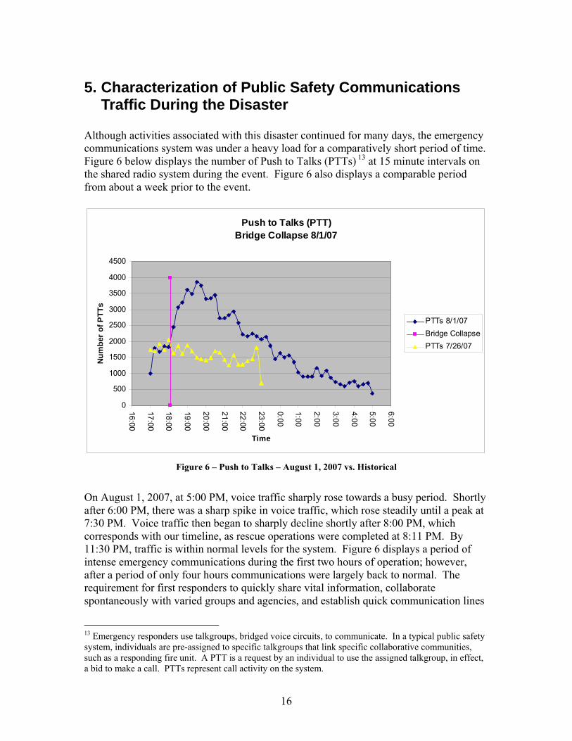
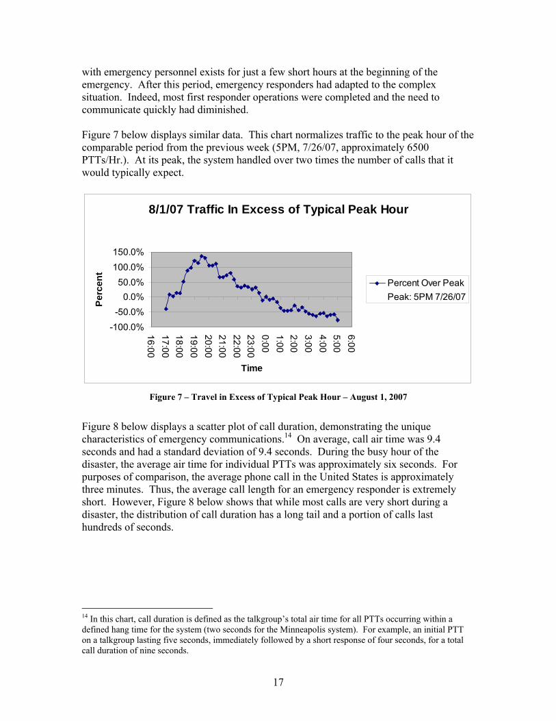
with emergency personnel exists for just a few short hours at the beginning of the emergency. After this period, emergency responders had adapted to the complex situation. Indeed, most first responder operations were completed and the need to communicate quickly had diminished. Figure 7 below displays similar data. This chart normalizes traffic to the peak hour of the comparable period from the previous week (5PM, 7/26/07, approximately 6500 PTTs/Hr.). At its peak, the system handled over two times the number of calls that it would typically expect.

8/1/07 Traffic In Excess of Typical Peak Hour

-100.0%-50.0%

0.0%50.0%

100.0%150.0%

16:0017:0018:0019:0020:0021:0022:0023:000:001:002:003:004:005:006:00

Time

Perc

ent

Percent Over PeakPeak: 5PM 7/26/07

Figure 7 – Travel in Excess of Typical Peak Hour – August 1, 2007

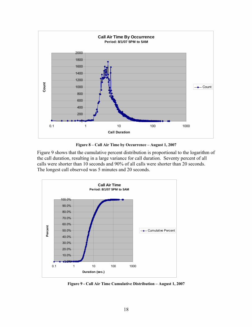
Figure 8 below displays a scatter plot of call duration, demonstrating the unique characteristics of emergency communications.14 On average, call air time was 9.4 seconds and had a standard deviation of 9.4 seconds. During the busy hour of the disaster, the average air time for individual PTTs was approximately six seconds. For purposes of comparison, the average phone call in the United States is approximately three minutes. Thus, the average call length for an emergency responder is extremely short. However, Figure 8 below shows that while most calls are very short during a disaster, the distribution of call duration has a long tail and a portion of calls last hundreds of seconds.

14 In this chart, call duration is defined as the talkgroup’s total air time for all PTTs occurring within a defined hang time for the system (two seconds for the Minneapolis system). For example, an initial PTT on a talkgroup lasting five seconds, immediately followed by a short response of four seconds, for a total call duration of nine seconds.

18

Call Air Time By OccurrencePeriod: 8/1/07 5PM to 5AM

0

200

400

600

800

1000

1200

1400

1600

1800

2000

0.1 1 10 100 1000

Call Duration

Cou

nt

Count

Figure 8 – Call Air Time by Occurrence – August 1, 2007

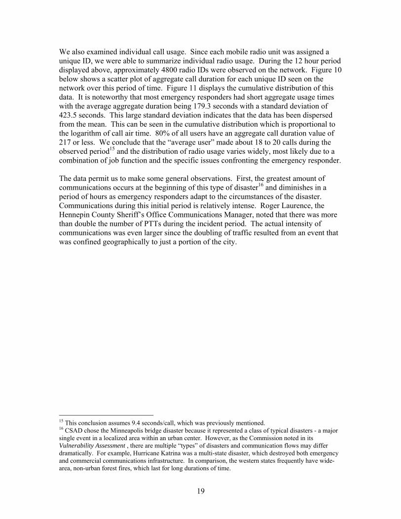
Figure 9 shows that the cumulative percent distribution is proportional to the logarithm of the call duration, resulting in a large variance for call duration. Seventy percent of all calls were shorter than 10 seconds and 90% of all calls were shorter than 20 seconds. The longest call observed was 5 minutes and 20 seconds.

Figure 9 - Call Air Time Cumulative Distribution – August 1, 2007

Call Air TimePeriod: 8/1/07 5PM to 5AM

0.0%

10.0%

20.0%

30.0%

40.0%

50.0%

60.0%

70.0%

80.0%

90.0%

100.0%

0.1 1 10 100 1000

Duration (sec.)

Perc

ent

Cumulative Percent

19

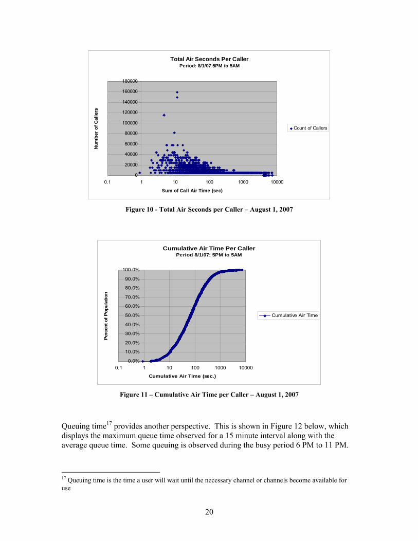
We also examined individual call usage. Since each mobile radio unit was assigned a unique ID, we were able to summarize individual radio usage. During the 12 hour period displayed above, approximately 4800 radio IDs were observed on the network. Figure 10 below shows a scatter plot of aggregate call duration for each unique ID seen on the network over this period of time. Figure 11 displays the cumulative distribution of this data. It is noteworthy that most emergency responders had short aggregate usage times with the average aggregate duration being 179.3 seconds with a standard deviation of 423.5 seconds. This large standard deviation indicates that the data has been dispersed from the mean. This can be seen in the cumulative distribution which is proportional to the logarithm of call air time. 80% of all users have an aggregate call duration value of 217 or less. We conclude that the “average user” made about 18 to 20 calls during the observed period15 and the distribution of radio usage varies widely, most likely due to a combination of job function and the specific issues confronting the emergency responder. The data permit us to make some general observations. First, the greatest amount of communications occurs at the beginning of this type of disaster16 and diminishes in a period of hours as emergency responders adapt to the circumstances of the disaster. Communications during this initial period is relatively intense. Roger Laurence, the Hennepin County Sheriff’s Office Communications Manager, noted that there was more than double the number of PTTs during the incident period. The actual intensity of communications was even larger since the doubling of traffic resulted from an event that was confined geographically to just a portion of the city.

15 This conclusion assumes 9.4 seconds/call, which was previously mentioned. 16 CSAD chose the Minneapolis bridge disaster because it represented a class of typical disasters - a major single event in a localized area within an urban center. However, as the Commission noted in its Vulnerability Assessment , there are multiple “types” of disasters and communication flows may differ dramatically. For example, Hurricane Katrina was a multi-state disaster, which destroyed both emergency and commercial communications infrastructure. In comparison, the western states frequently have wide-area, non-urban forest fires, which last for long durations of time.

20

Total Air Seconds Per CallerPeriod: 8/1/07 5PM to 5AM

0

20000

40000

60000

80000

100000

120000

140000

160000

180000

0.1 1 10 100 1000 10000

Sum of Call Air Time (sec)

Num

ber

of C

alle

rs

Count of Callers

Figure 10 - Total Air Seconds per Caller – August 1, 2007

Cumulative Air Time Per CallerPeriod 8/1/07: 5PM to 5AM

0.0%

10.0%

20.0%

30.0%

40.0%

50.0%

60.0%

70.0%

80.0%

90.0%

100.0%

0.1 1 10 100 1000 10000

Cumulative Air Time (sec.)

Perc

ent o

f Pop

ulat

ion

Cumulative Air Time

Figure 11 – Cumulative Air Time per Caller – August 1, 2007

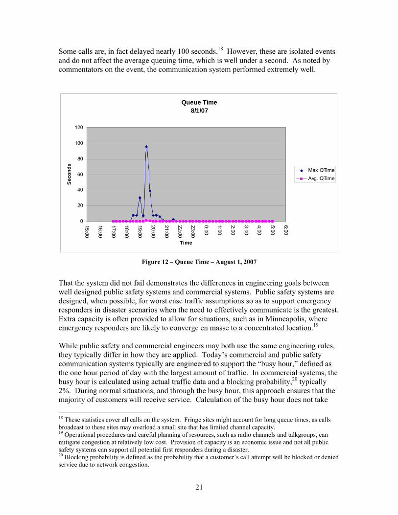
Queuing time17 provides another perspective. This is shown in Figure 12 below, which displays the maximum queue time observed for a 15 minute interval along with the average queue time. Some queuing is observed during the busy period 6 PM to 11 PM.

17 Queuing time is the time a user will wait until the necessary channel or channels become available for use

21

Some calls are, in fact delayed nearly 100 seconds.18 However, these are isolated events and do not affect the average queuing time, which is well under a second. As noted by commentators on the event, the communication system performed extremely well.

Queue Time8/1/07

0

20

40

60

80

100

120

15:00

16:00

17:00

18:00

19:00

20:00

21:00

22:00

23:00

0:00

1:00

2:00

3:00

4:00

5:00

6:00

Time

Seco

nds

Max QTimeAvg. QTime

Figure 12 – Queue Time – August 1, 2007

That the system did not fail demonstrates the differences in engineering goals between well designed public safety systems and commercial systems. Public safety systems are designed, when possible, for worst case traffic assumptions so as to support emergency responders in disaster scenarios when the need to effectively communicate is the greatest. Extra capacity is often provided to allow for situations, such as in Minneapolis, where emergency responders are likely to converge en masse to a concentrated location.19 While public safety and commercial engineers may both use the same engineering rules, they typically differ in how they are applied. Today’s commercial and public safety communication systems typically are engineered to support the “busy hour,” defined as the one hour period of day with the largest amount of traffic. In commercial systems, the busy hour is calculated using actual traffic data and a blocking probability,20 typically 2%. During normal situations, and through the busy hour, this approach ensures that the majority of customers will receive service. Calculation of the busy hour does not take 18 These statistics cover all calls on the system. Fringe sites might account for long queue times, as calls broadcast to these sites may overload a small site that has limited channel capacity. 19 Operational procedures and careful planning of resources, such as radio channels and talkgroups, can mitigate congestion at relatively low cost. Provision of capacity is an economic issue and not all public safety systems can support all potential first responders during a disaster. 20 Blocking probability is defined as the probability that a customer’s call attempt will be blocked or denied service due to network congestion.

22

into account worst case events where traffic may be generated in excess of the busy hour. In a commercial environment, worst case scenarios creating heavy traffic loads can range from car accidents (for cellular traffic), disasters such as floods or storms, or radio or TV call-in triggered events where large numbers of people direct calls to specific locations. During these abnormal call periods, calls are simply blocked. 4G commercial technologies should have the capability to assign priority access dynamically to various types of users, thereby improving emergency responders’ access to communications services during disasters. In the public safety environment a strategy of call blocking during the busy hour is not acceptable. Accordingly, LMR design parameters like busy hour load may be adjusted to reflect worst case scenarios in an attempt to engineer communications systems for traffic loads during emergency events. Thus a public safety engineer, for example, may factor into the busy hour the impact of extra units responding into the area. The use of talkgroups (basically a form of call conferencing) by public safety entities is also different from the counterpart used in the commercial world. As anyone who has used commercial conference calling understands, as a general rule the larger the number of participants on the call, the more difficult it becomes to carry on a conversation. This results from a lack of discipline and organization among the participants on most conference calls. Commercial conference calls therefore typically involve small numbers of people. Both the military and public safety entities have determined, however, that if more organizations can be brought into the conference, and if people communicate among themselves in a disciplined fashion, far larger numbers of people can be joined effectively on a single conference call. As a result, talkgroups are far larger in the public safety community than their equivalents in the commercial world. Public safety representatives have pointed out that some talkgroups support hundreds of people. Although a disciplined approach can dramatically increase the effectiveness of talkgroups, ultimately if the talkgroup is to remain interactive (as opposed to a pure broadcast channel where a dedicated speaker can talk to effectively unlimited number of people), utilization21 of the talkgroup must be low enough to allow a user to grab or bid for the talkgroup in an efficient manner. If utilization is too high, users become frustrated in attempting to communicate over the talkgroup. Roger Laurence, the Hennepin County Communications Manager, stated that they use a figure of 30% utilization as a figure of merit. Beyond this level, users believe that the talkgroup is being degraded.22

21 Utilization is defined as the percent of time that a channel is occupied. 22 Roger Laurence, Manager, Hennepin County Communications, interview with FCC staff preparing this report.

23

6. Performance Modeling and Evaluation of Trunked LMR Systems

By developing and calibrating a system model that includes appropriate parameters and performance metrics, we intended to evaluate the performance and capacity of the Minneapolis LMR system during the disaster and to analyze trunked LMR systems more generally, ultimately providing design guidelines for systems of this type.

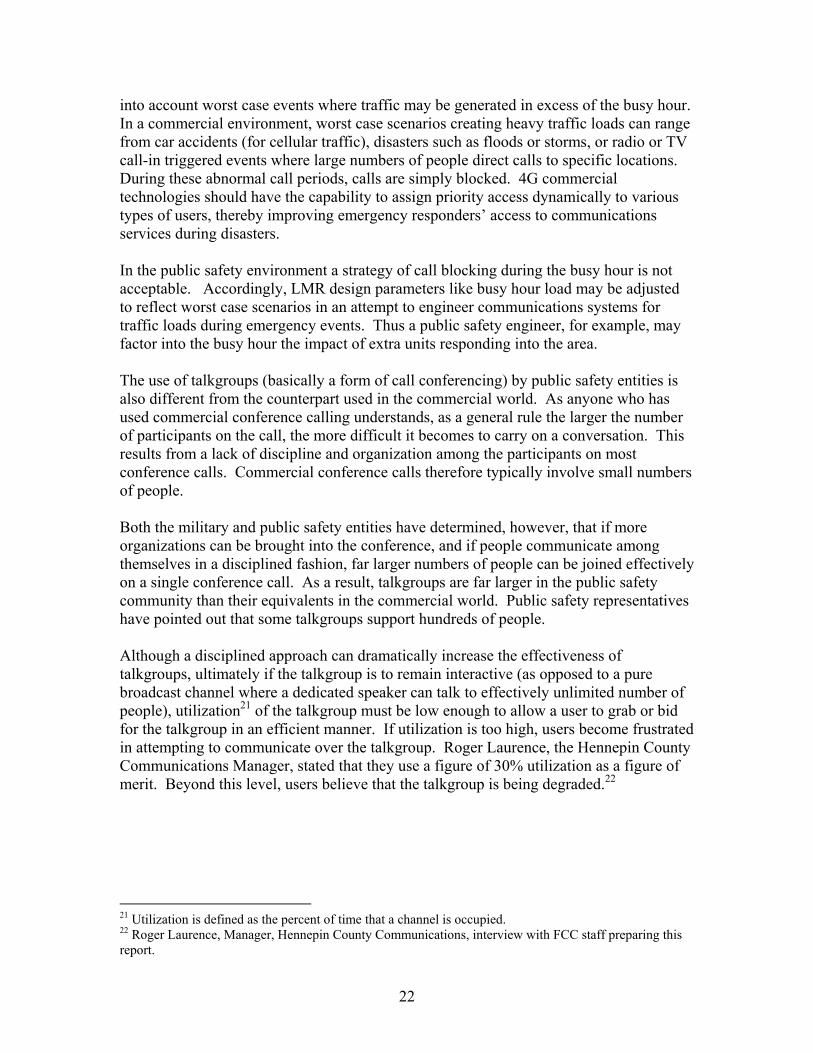
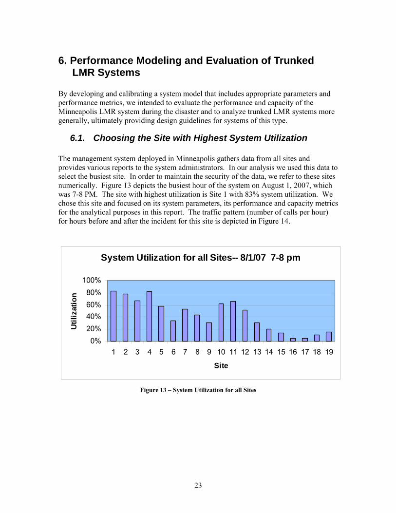
6.1. Choosing the Site with Highest System Utilization The management system deployed in Minneapolis gathers data from all sites and provides various reports to the system administrators. In our analysis we used this data to select the busiest site. In order to maintain the security of the data, we refer to these sites numerically. Figure 13 depicts the busiest hour of the system on August 1, 2007, which was 7-8 PM. The site with highest utilization is Site 1 with 83% system utilization. We chose this site and focused on its system parameters, its performance and capacity metrics for the analytical purposes in this report. The traffic pattern (number of calls per hour) for hours before and after the incident for this site is depicted in Figure 14.

System Utilization for all Sites-- 8/1/07 7-8 pm

0%20%40%60%80%

100%

1 2 3 4 5 6 7 8 9 10 11 12 13 14 15 16 17 18 19

Site

Utili

zatio

n

Figure 13 – System Utilization for all Sites

24

Site 1 Call Requests

4,512

7,852

10,077

6,803

4,6304,107

5,660

7,739

5,678

-

2,000

4,000

6,000

8,000

10,000

12,000C

all R

eque

sts

07/26/07 03:00 PM 8/1/07 5:00 PM 8/1/07 6:00 PM 8/1/07 7:00 PM 8/1/07 8:00 PM

8/1/07 9:00 PM 8/1/07 10:00 PM 8/1/07 11:00 PM 8/1/07 12:00 PM

Figure 14 – Cell 1 Call Requests

6.2. Systems Modeling LMR systems support one-to-many communications. Users are organized into talkgroups in which only one user may talk at a time while others are listening. In a conventional system, a talkgroup is assigned to a single channel in a static manner. In a trunked LMR system, a talkgroup gets access to a channel from a pool of shared channels. If a channel is not available, the talkgroup’s request for access goes into a central queue. The various approaches to model the current system architecture provide different degrees of insight and pose different analysis complexities. We chose an approach that balanced these two extremes. Appendix A documents the modeling approach and analysis process in detail. Two factors influence the end-to-end LMR performance experienced by a user: performance of the central queue, which we also refer to as the performance of the system, and performance of the talkgroup of which the user is a member.

25

6.2.1. System Performance The LMR system performance is determined by the physical queue in the control system that is used for channel assignment purposes in a simulcast group, referred to here as the “central queue.” Our performance analysis of this queue provides results for any generic trunked LMR system, including the Minneapolis system. The central queue follows an Erlang C model23 with N, the number of channels, λ, the mean rate of call arrival within a simulcast group, and 1/µ, the mean call duration. The total offered traffic load is defined to be A= λ/µ erlang. The system utilization is defined to be ρ= λ/(Nµ), which should be less than one to ensure system stability. We calibrated our model using data from the Minneapolis disaster by calculating the statistical mean of call interarrival and call duration from the empirical data. Calibration ensures that the fundamental parameters of the model are pegged to real, observed data and gives us confidence that the parameters can be altered to predict system performance under different conditions. System performance metrics based on the statistics of the central queue include waiting probability (probability of a call waiting in the queue to grab a channel), PW, and average waiting time (or queuing delay) for those calls that have to wait in the central queue, WC. The waiting probability, PW is the probability that a call upon its arrival has to wait in the central queue for channel access. Average waiting time (WC), otherwise known as queuing delay, is the average waiting time for those calls that have to wait in the central queue before being assigned a channel. This is different than the average waiting time for all calls, which also includes those that do not have to wait in the queue. WC is equal to the waiting time for all calls divided by the waiting probability, PW. The performance metrics introduced here are used to define the Grade of Service (GoS) for LMR systems. GoS sets objective thresholds for performance metrics. For example, the percentage of calls that experience queuing delays beyond a certain threshold would be a good candidate for a GoS benchmark. The hypothetical benchmark might be selected such that no more than 2% of calls experience a wait time of 3 seconds or more. Mathematically, this translates to the probability of W≥3 seconds being 0.02, which is obtained from the statistics of W that are embedded in our system model.

In this report we also discuss system design and capacity considerations for a trunked LMR system. We determine, based on a predefined GoS, the allowable region of operation, i.e., the required number of channels (or spectrum) versus system utilization. Similarly, we determine, based on a predefined GoS, the capacity regions, i.e., the required number of channels (or spectrum) versus traffic intensity (erlang).

23 A queuing system with exponential interarrival, exponential service time, and N servers – Queuing Systems, Volume 1: Theory, Leonard Kleinrock, 1975.

26

6.2.2. Talkgroup Performance While system performance is a necessary element of the quality of service perceived by a user, it is not a complete description. The quality of service perceived by a user also depends on the talkgroup to which the user is assigned. Talkgroup quality of service, for instance, can be adversely impacted for oversubscribed talkgroups, even if the overall system is lightly loaded with traffic. Under such conditions, users with desire to talk have to compete with others in the talkgroup and may have to wait long periods of time in order to talk. Long waits hamper emergency responders in their critical duties. We model such user annoyance through locally measurable waiting time of a virtual queue. In other words, the locally perceived user waiting time serves as a surrogate for user annoyance. The talkgroup utilization, which is different than the system utilization as defined earlier, is defined to be ρ= λ1/µ, where λ1 is the mean rate of call arrivals from the talkgroup members, and 1/µ is the mean call duration. When there is no delay in the central queue, there is a benchmark threshold for talkgroup utilization beyond which the talkgroup performance is not acceptable. Using the model described in Appendix A and in particular, the notion of locally perceived user waiting time, we calculate the talkgroup utilization threshold for the same system under heavy loads. This topic is further discussed in a later section.

6.3. Analysis and Discussion of Minneapolis LMR System

6.3.1. Data Collection We collected field data for the system, which is configured to maintain a log of call and system activities for up to two years. The time-stamped data contains information about the duration of call and push-to-talk (PTT) activities. The system log also contains time-stamped information about talkgroups usage, simulcast groups, sites, and radio IDs.

Past System Performance and Calibration of Model We used the system log data to analyze the performance of the system during normal operations and directly after the bridge collapse. Additionally, we used the data to calibrate the model described earlier. The calibrated model allowed us to predict the future performance of the system and provide capacity and performance design guidelines for similar systems. Using the real data as well as our model, we calculated the system’s performance for various scenarios using the simulcast group that carried the most traffic after the bridge collapse. Three sets of data were collected from the system for this site. One for a busy hour at 3 PM on July 26, 2007, one for the hour before the incident at 5 PM on August 1,

27

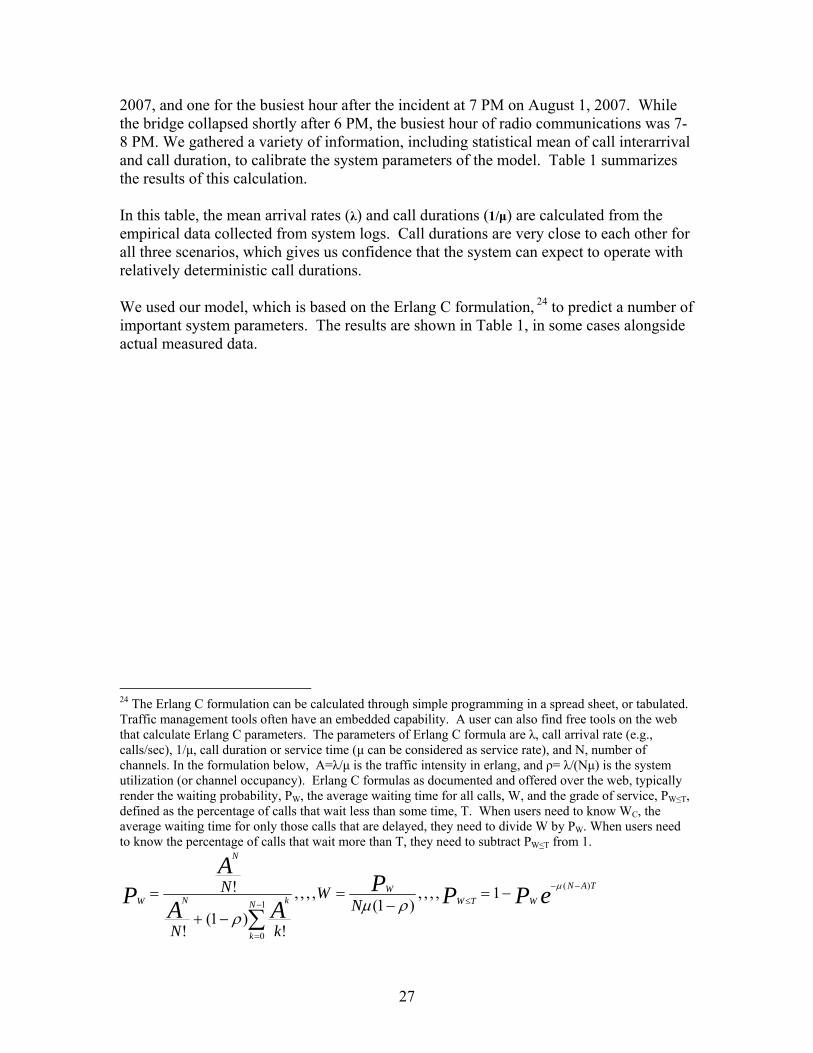
2007, and one for the busiest hour after the incident at 7 PM on August 1, 2007. While the bridge collapsed shortly after 6 PM, the busiest hour of radio communications was 7-8 PM. We gathered a variety of information, including statistical mean of call interarrival and call duration, to calibrate the system parameters of the model. Table 1 summarizes the results of this calculation. In this table, the mean arrival rates (λ) and call durations (1/µ) are calculated from the empirical data collected from system logs. Call durations are very close to each other for all three scenarios, which gives us confidence that the system can expect to operate with relatively deterministic call durations. We used our model, which is based on the Erlang C formulation, 24 to predict a number of important system parameters. The results are shown in Table 1, in some cases alongside actual measured data.

24 The Erlang C formulation can be calculated through simple programming in a spread sheet, or tabulated. Traffic management tools often have an embedded capability. A user can also find free tools on the web that calculate Erlang C parameters. The parameters of Erlang C formula are λ, call arrival rate (e.g., calls/sec), 1/µ, call duration or service time (µ can be considered as service rate), and N, number of channels. In the formulation below, A=λ/µ is the traffic intensity in erlang, and ρ= λ/(Nµ) is the system utilization (or channel occupancy). Erlang C formulas as documented and offered over the web, typically render the waiting probability, PW, the average waiting time for all calls, W, and the grade of service, PW≤T, defined as the percentage of calls that wait less than some time, T. When users need to know WC, the average waiting time for only those calls that are delayed, they need to divide W by PW. When users need to know the percentage of calls that wait more than T, they need to subtract PW≤T from 1.

ePPPAA

AP TAN

WTWW

N

k

kN

N

W NW

kN

N )(

1

0

1,,,,)1(

,,,,

!)1(

!

! −−

≤−

=

−=−

=

−+

=

∑

µ

ρµρ

28

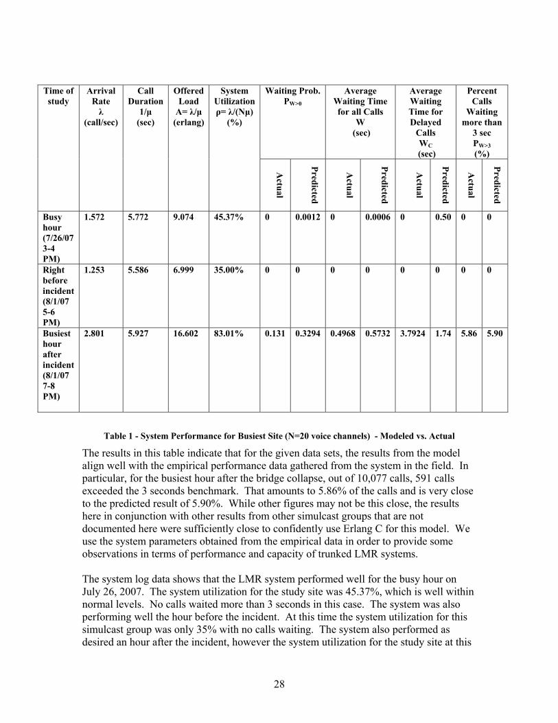
Table 1 - System Performance for Busiest Site (N=20 voice channels) - Modeled vs. Actual

The results in this table indicate that for the given data sets, the results from the model align well with the empirical performance data gathered from the system in the field. In particular, for the busiest hour after the bridge collapse, out of 10,077 calls, 591 calls exceeded the 3 seconds benchmark. That amounts to 5.86% of the calls and is very close to the predicted result of 5.90%. While other figures may not be this close, the results here in conjunction with other results from other simulcast groups that are not documented here were sufficiently close to confidently use Erlang C for this model. We use the system parameters obtained from the empirical data in order to provide some observations in terms of performance and capacity of trunked LMR systems. The system log data shows that the LMR system performed well for the busy hour on July 26, 2007. The system utilization for the study site was 45.37%, which is well within normal levels. No calls waited more than 3 seconds in this case. The system was also performing well the hour before the incident. At this time the system utilization for this simulcast group was only 35% with no calls waiting. The system also performed as desired an hour after the incident, however the system utilization for the study site at this

Waiting Prob.PW>0

Average Waiting Time for all Calls

W (sec)

Average Waiting Time for Delayed

Calls WC

(sec)

Percent Calls

Waiting more than

3 sec PW>3 (%)

Time of study

Arrival Rate λ

(call/sec)

Call Duration

1/µ (sec)

Offered Load

A= λ/µ (erlang)

System Utilization ρ= λ/(Nµ)

(%)

Actual

Predicted

Actual

Predicted

Actual

Predicted

Actual

Predicted

Busy hour (7/26/07 3-4 PM)

1.572 5.772 9.074 45.37% 0 0.0012 0 0.0006 0 0.50 0 0

Right before incident (8/1/07 5-6 PM)

1.253 5.586 6.999 35.00% 0 0 0 0 0 0 0 0

Busiest hour after incident (8/1/07 7-8 PM)

2.801 5.927 16.602 83.01% 0.131 0.3294 0.4968 0.5732 3.7924 1.74 5.86 5.90

29

time went up to 83.01%. About 5.9% of the calls also had to wait more than 3 seconds in this case, which exceeds the desired Grade of Service for normal operations but was still satisfactory according to accounts from local emergency responders considering the extraordinary nature of the incident. In fact, they claimed that they could have tolerated delays of up to 10 seconds before declaring the system critically overloaded.25 In fact, they claimed that they could have tolerated delays of up to 10 seconds before declaring the system unusable. Accordingly, for this site we set the GoS to be 2% of calls experiencing more than 10 seconds of delay. This relaxed GoS requirement permits system utilizations of as high as 90.1%.

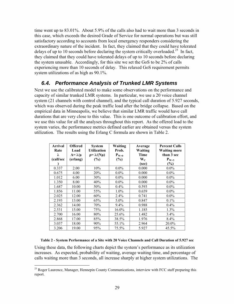
6.4. Performance Analysis of Trunked LMR Systems Next we use the calibrated model to make some observations on the performance and capacity of similar trunked LMR systems. In particular, we use a 20 voice channel system (21 channels with control channel), and the typical call duration of 5.927 seconds, which was observed during the peak traffic load after the bridge collapse. Based on the empirical data in Minneapolis, we believe that similar LMR traffic would have call durations that are very close to this value. This is one outcome of calibration effort, and we use this value for all the analyses throughout this report. As the offered load to the system varies, the performance metrics defined earlier are obtained versus the system utilization. The results using the Erlang C formula are shown in Table 2.

Table 2 - System Performance of a Site with 20 Voice Channels and Call Duration of 5.927 sec

Using these data, the following charts depict the system’s performance as its utilization increases. As expected, probability of waiting, average waiting time, and percentage of calls waiting more than 3 seconds, all increase sharply at higher system utilizations. The 25 Roger Laurence, Manager, Hennepin County Communications, interview with FCC staff preparing this report.

Arrival Rate λ

(call/sec)

Offered Load

A= λ/µ (erlang)

System Utilization ρ= λ/(Nµ)

(%)

Waiting Prob. PW>0 (%)

Average Waiting

Time WC

(sec)

Percent Calls Waiting more

than 3 sec PW>3 (%)

0.337 2.00 10% 0.0% 0.000 0.0% 0.675 4.00 20% 0.0% 0.000 0.0% 1.012 6.00 30% 0.0% 0.000 0.0% 1.350 8.00 40% 0.0% 0.000 0.0% 1.687 10.00 50% 0.4% 0.593 0.0% 1.856 11.00 55% 1.0% 0.659 0.0% 2.025 12.00 60% 2.4% 0.741 0.0% 2.193 13.00 65% 5.0% 0.847 0.1% 2.362 14.00 70% 9.4% 0.988 0.4% 2.531 15.00 75% 16.0% 1.185 1.3% 2.700 16.00 80% 25.6% 1.482 3.4% 2.868 17.00 85% 38.5% 1.976 8.4% 3.037 18.00 90% 55.1% 2.964 20.0% 3.206 19.00 95% 75.5% 5.927 45.5%

30

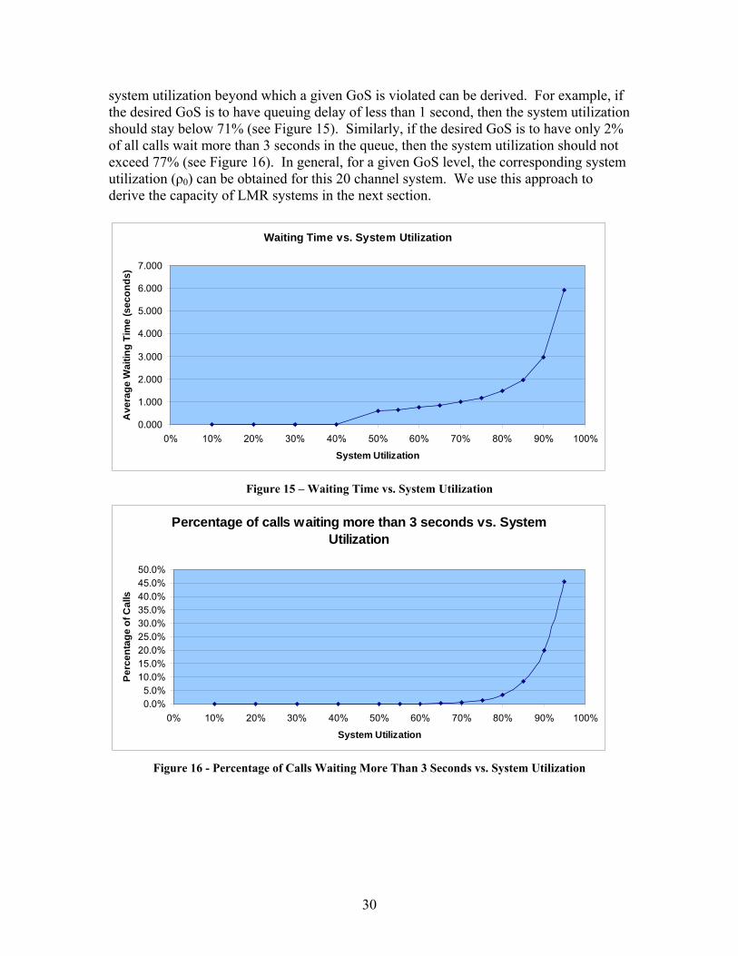
system utilization beyond which a given GoS is violated can be derived. For example, if the desired GoS is to have queuing delay of less than 1 second, then the system utilization should stay below 71% (see Figure 15). Similarly, if the desired GoS is to have only 2% of all calls wait more than 3 seconds in the queue, then the system utilization should not exceed 77% (see Figure 16). In general, for a given GoS level, the corresponding system utilization (ρ0) can be obtained for this 20 channel system. We use this approach to derive the capacity of LMR systems in the next section.

Waiting Time vs. System Utilization

0.000

1.000

2.000

3.000

4.000

5.000

6.000

7.000

0% 10% 20% 30% 40% 50% 60% 70% 80% 90% 100%

System Utilization

Ave

rage

Wai

ting

Tim

e (s

econ

ds)

Figure 15 – Waiting Time vs. System Utilization

Percentage of calls waiting more than 3 seconds vs. System Utilization

0.0%5.0%

10.0%15.0%20.0%25.0%30.0%35.0%40.0%45.0%50.0%

0% 10% 20% 30% 40% 50% 60% 70% 80% 90% 100%

System Utilization

Perc

enta

ge o

f Cal

ls

Figure 16 - Percentage of Calls Waiting More Than 3 Seconds vs. System Utilization

31

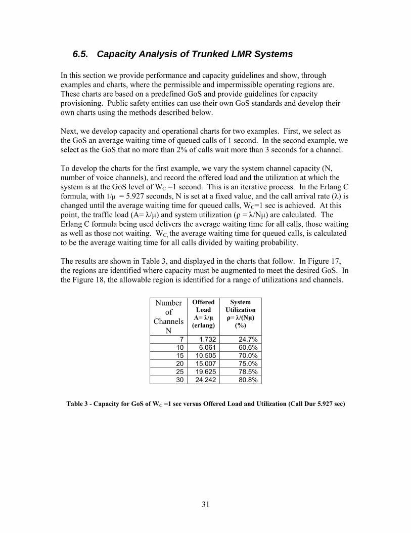
6.5. Capacity Analysis of Trunked LMR Systems In this section we provide performance and capacity guidelines and show, through examples and charts, where the permissible and impermissible operating regions are. These charts are based on a predefined GoS and provide guidelines for capacity provisioning. Public safety entities can use their own GoS standards and develop their own charts using the methods described below. Next, we develop capacity and operational charts for two examples. First, we select as the GoS an average waiting time of queued calls of 1 second. In the second example, we select as the GoS that no more than 2% of calls wait more than 3 seconds for a channel. To develop the charts for the first example, we vary the system channel capacity (N, number of voice channels), and record the offered load and the utilization at which the system is at the GoS level of WC =1 second. This is an iterative process. In the Erlang C formula, with 1/µ = 5.927 seconds, N is set at a fixed value, and the call arrival rate (λ) is changed until the average waiting time for queued calls, WC=1 sec is achieved. At this point, the traffic load (A= λ/µ) and system utilization (ρ = λ/Nµ) are calculated. The Erlang C formula being used delivers the average waiting time for all calls, those waiting as well as those not waiting. WC, the average waiting time for queued calls, is calculated to be the average waiting time for all calls divided by waiting probability. The results are shown in Table 3, and displayed in the charts that follow. In Figure 17, the regions are identified where capacity must be augmented to meet the desired GoS. In the Figure 18, the allowable region is identified for a range of utilizations and channels.

Table 3 - Capacity for GoS of WC =1 sec versus Offered Load and Utilization (Call Dur 5.927 sec)

Number of

ChannelsN

Offered Load

A= λ/µ (erlang)

System Utilization ρ= λ/(Nµ)

(%)

7 1.732 24.7%10 6.061 60.6%15 10.505 70.0%20 15.007 75.0%25 19.625 78.5%30 24.242 80.8%

32

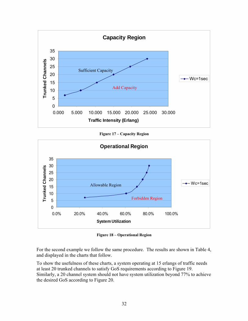
Figure 17 – Capacity Region

Figure 18 – Operational Region

For the second example we follow the same procedure. The results are shown in Table 4, and displayed in the charts that follow.

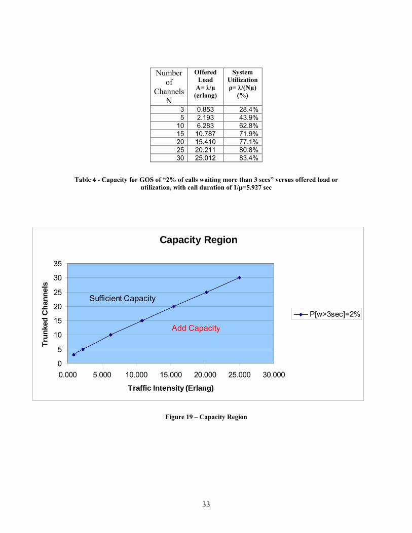
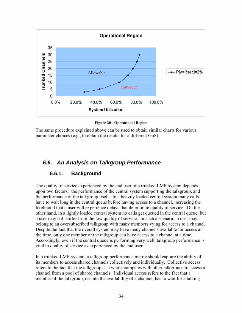
To show the usefulness of these charts, a system operating at 15 erlangs of traffic needs at least 20 trunked channels to satisfy GoS requirements according to Figure 19. Similarly, a 20 channel system should not have system utilization beyond 77% to achieve the desired GoS according to Figure 20.

Capacity Region

0

5

10

15

20

25

30

35

0.000 5.000 10.000 15.000 20.000 25.000 30.000

Traffic Intensity (Erlang)

Trun

ked

Cha

nnel

s

Wc=1sec

Add Capacity

Sufficient Capacity

Operational Region

05

1015

20253035

0.0% 20.0% 40.0% 60.0% 80.0% 100.0%

System Utilization

Trun

ked

Cha

nnel

s

Wc=1secAllowable Region

Forbidden Region

33

Table 4 - Capacity for GOS of “2% of calls waiting more than 3 secs” versus offered load or utilization, with call duration of 1/µ=5.927 sec

Figure 19 – Capacity Region

Number of

ChannelsN

Offered Load

A= λ/µ (erlang)

System Utilization ρ= λ/(Nµ)

(%)

3 0.853 28.4%5 2.193 43.9%

10 6.283 62.8%15 10.787 71.9%20 15.410 77.1%25 20.211 80.8%30 25.012 83.4%

Capacity Region

0

5

10

15

20

25

30

35

0.000 5.000 10.000 15.000 20.000 25.000 30.000

Traffic Intensity (Erlang)

Trun

ked

Cha

nnel

s

P[w>3sec]=2%

Sufficient Capacity

Add Capacity

34

Figure 20 - Operational Region

The same procedure explained above can be used to obtain similar charts for various parameter choices (e.g., to obtain the results for a different GoS).

6.6. An Analysis on Talkgroup Performance

6.6.1. Background The quality of service experienced by the end user of a trunked LMR system depends upon two factors: the performance of the central system supporting the talkgroup, and the performance of the talkgroup itself. In a heavily loaded central system many calls have to wait long in the central queue before having access to a channel, increasing the likelihood that a user will experience delays that deteriorate quality of service. On the other hand, in a lightly loaded central system no calls get queued in the central queue, but a user may still suffer from the low quality of service. In such a scenario, a user may belong to an oversubscribed talkgroup with many members vying for access to a channel. Despite the fact that the overall system may have many channels available for access at the time, only one member of the talkgroup can have access to a channel at a time. Accordingly, even if the central queue is performing very well, talkgroup performance is vital to quality of service as experienced by the end user. In a trunked LMR system, a talkgroup performance metric should capture the ability of its members to access shared channels collectively and individually. Collective access refers to the fact that the talkgroup as a whole competes with other talkgroups to access a channel from a pool of shared channels. Individual access refers to the fact that a member of the talkgroup, despite the availability of a channel, has to wait for a talking

Operational Region

05

101520253035

0.0% 20.0% 40.0% 60.0% 80.0% 100.0%

System Utilization

Trun

ked

Cha

nnel

s

P[w>3sec]=2%Allowable

Forbidden

35

member to finish talking before speaking. Such waiting time is annoying to talkgroup members and adversely impacts effective communications at times of heavy usage. In other words, even if the overall system is lightly loaded with traffic and plenty of trunked channels are available, a poor design for talkgroup arrangements (such as oversubscription) can cause performance degradation for users.

6.6.2. Analysis While we do not have a benchmark for talkgroup performance, we adopt 30% talkgroup utilization as a threshold beyond which the user perceived quality deteriorates. We have been advised that beyond this level effective communication suffers and users get annoyed.26 We can easily translate this level of utilization to delays locally perceived (or level of annoyance experienced) by a user within a talkgroup.27 We further assume that the 30% talkgroup utilization threshold is for the case in which the system utilization is low,28 and a talkgroup always has access to a channel without any delay. This equates to performance of a talkgroup operating in a conventional system in which a channel is permanently assigned to a talkgroup. Later in this section we develop a formula and calculate the talkgroup utilization threshold for higher system utilizations.

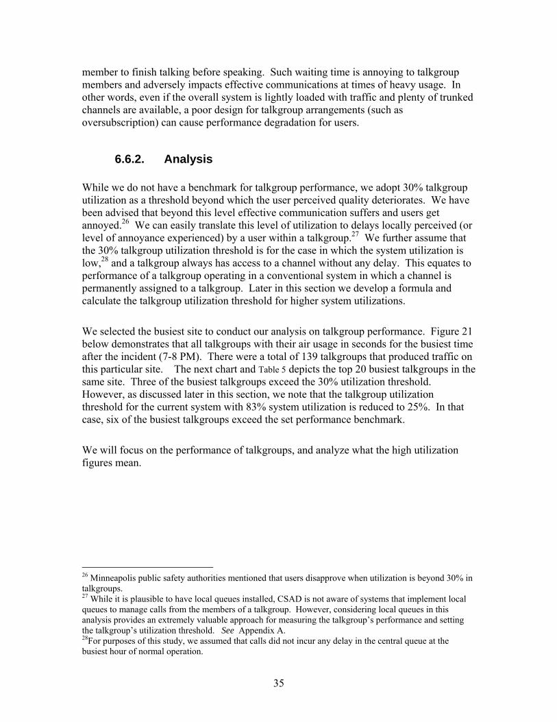
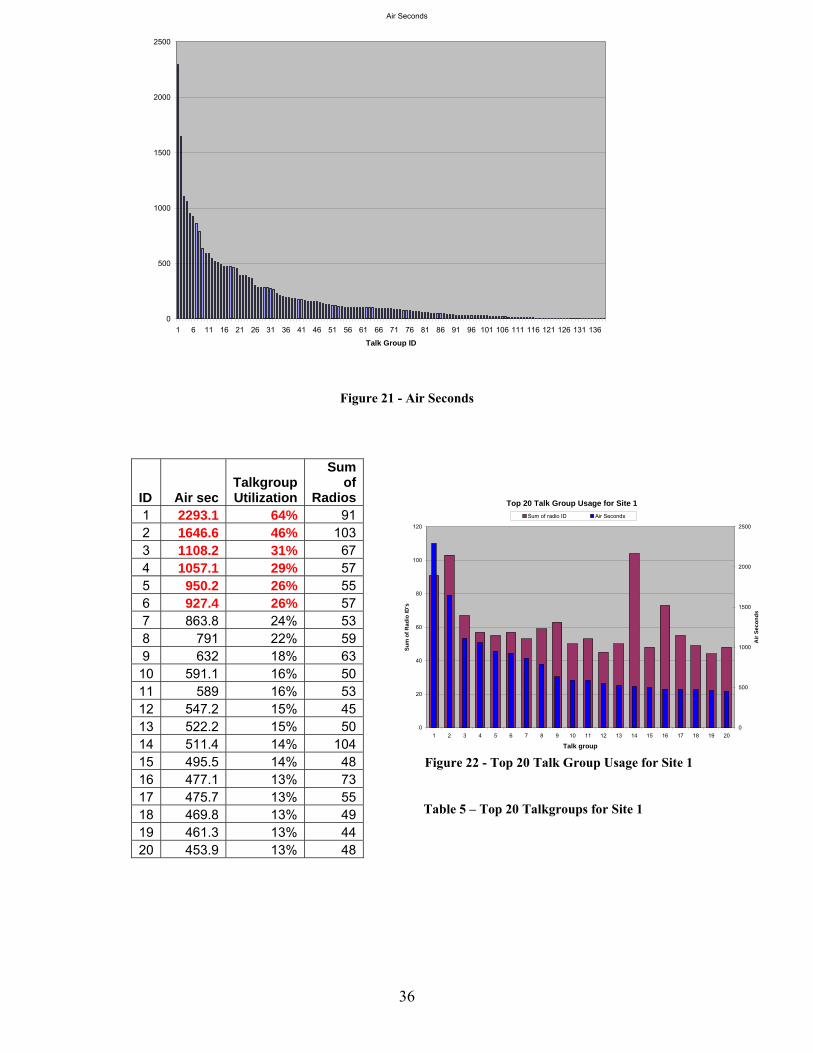
We selected the busiest site to conduct our analysis on talkgroup performance. Figure 21 below demonstrates that all talkgroups with their air usage in seconds for the busiest time after the incident (7-8 PM). There were a total of 139 talkgroups that produced traffic on this particular site. The next chart and Table 5 depicts the top 20 busiest talkgroups in the same site. Three of the busiest talkgroups exceed the 30% utilization threshold. However, as discussed later in this section, we note that the talkgroup utilization threshold for the current system with 83% system utilization is reduced to 25%. In that case, six of the busiest talkgroups exceed the set performance benchmark.

We will focus on the performance of talkgroups, and analyze what the high utilization figures mean.

26 Minneapolis public safety authorities mentioned that users disapprove when utilization is beyond 30% in talkgroups. 27 While it is plausible to have local queues installed, CSAD is not aware of systems that implement local queues to manage calls from the members of a talkgroup. However, considering local queues in this analysis provides an extremely valuable approach for measuring the talkgroup’s performance and setting the talkgroup’s utilization threshold. See Appendix A. 28For purposes of this study, we assumed that calls did not incur any delay in the central queue at the busiest hour of normal operation.

36

Figure 21 - Air Seconds

Figure 22 - Top 20 Talk Group Usage for Site 1

Table 5 – Top 20 Talkgroups for Site 1

ID Air sec Talkgroup Utilization

Sum of

Radios1 2293.1 64% 912 1646.6 46% 1033 1108.2 31% 674 1057.1 29% 575 950.2 26% 556 927.4 26% 577 863.8 24% 538 791 22% 599 632 18% 6310 591.1 16% 5011 589 16% 5312 547.2 15% 4513 522.2 15% 5014 511.4 14% 10415 495.5 14% 4816 477.1 13% 7317 475.7 13% 5518 469.8 13% 4919 461.3 13% 4420 453.9 13% 48

Air Seconds

0

500

1000

1500

2000

2500

1 6 11 16 21 26 31 36 41 46 51 56 61 66 71 76 81 86 91 96 101 106 111 116 121 126 131 136

Talk Group ID

Top 20 Talk Group Usage for Site 1

0

20

40

60

80

100

120

1 2 3 4 5 6 7 8 9 10 11 12 13 14 15 16 17 18 19 20

Talk group

Sum

of R

adio

ID's

0

500

1000

1500

2000

2500

Air

Seco

nds

Sum of radio ID Air Seconds

37

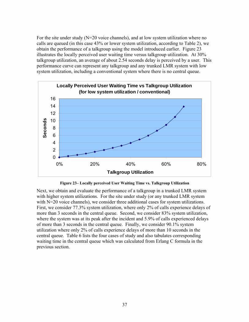
For the site under study (N=20 voice channels), and at low system utilization where no calls are queued (in this case 43% or lower system utilization, according to Table 2), we obtain the performance of a talkgroup using the model introduced earlier. Figure 23 illustrates the locally perceived user waiting time versus talkgroup utilization. At 30% talkgroup utilization, an average of about 2.54 seconds delay is perceived by a user. This performance curve can represent any talkgroup and any trunked LMR system with low system utilization, including a conventional system where there is no central queue.

Locally Perceived User Waiting Time vs Talkgroup Utilization(for low system utilization / conventional)

02468

10121416

0% 20% 40% 60% 80%

Talkgroup Utilization

Seco

nds

Figure 23– Locally perceived User Waiting Time vs. Talkgroup Utilization

Next, we obtain and evaluate the performance of a talkgroup in a trunked LMR system with higher system utilizations. For the site under study (or any trunked LMR system with N=20 voice channels), we consider three additional cases for system utilizations. First, we consider 77.3% system utilization, where only 2% of calls experience delays of more than 3 seconds in the central queue. Second, we consider 83% system utilization, where the system was at its peak after the incident and 5.9% of calls experienced delays of more than 3 seconds in the central queue. Finally, we consider 90.1% system utilization where only 2% of calls experience delays of more than 10 seconds in the central queue. Table 6 lists the four cases of study and also tabulates corresponding waiting time in the central queue which was calculated from Erlang C formula in the previous section.

38

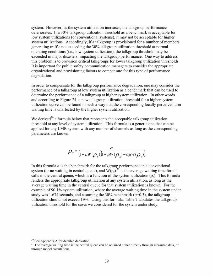
System Utilization W (waiting time for all calls in central queue), sec

Low (<43%) / Conventional 0 77.3% 0.264 83% 0.575 90.1% 1.674

Table 6 - System Utilization vs. Waiting Time in Central Queue

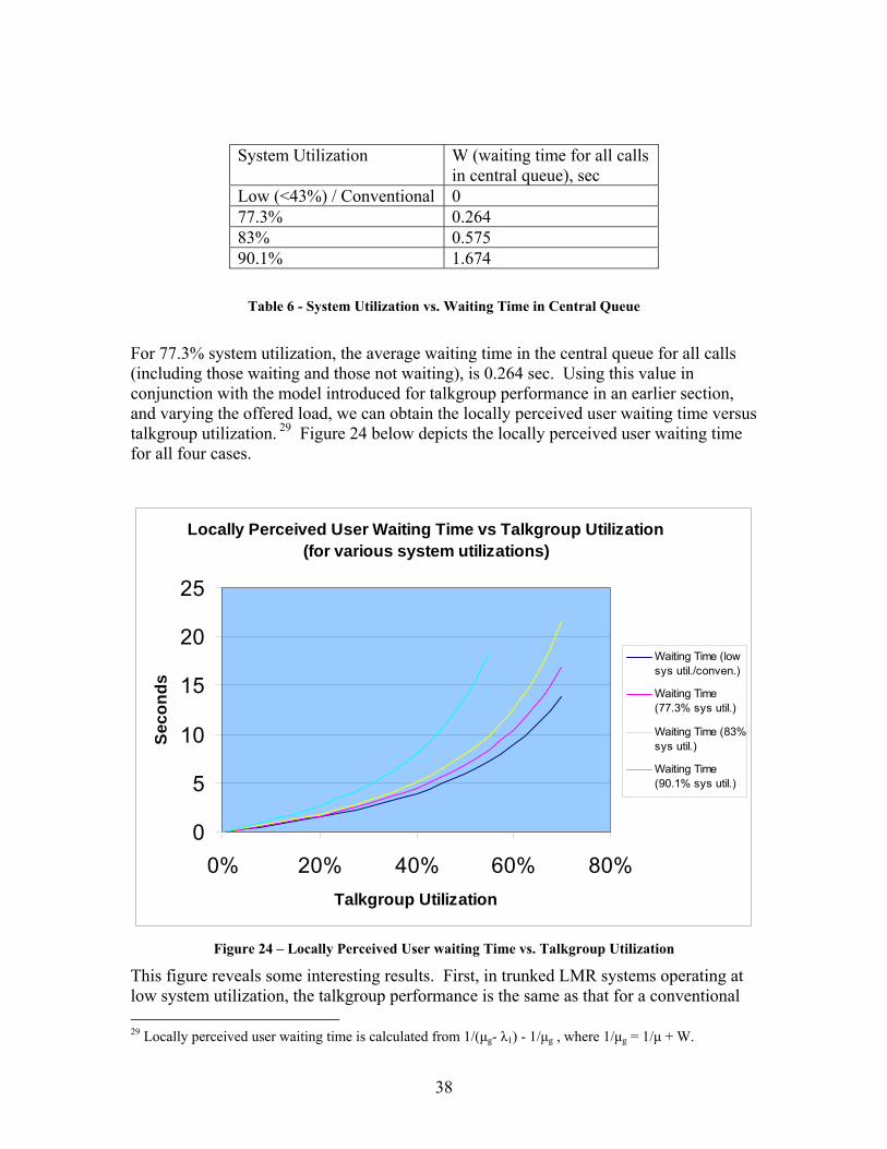
For 77.3% system utilization, the average waiting time in the central queue for all calls (including those waiting and those not waiting), is 0.264 sec. Using this value in conjunction with the model introduced for talkgroup performance in an earlier section, and varying the offered load, we can obtain the locally perceived user waiting time versus talkgroup utilization. 29 Figure 24 below depicts the locally perceived user waiting time for all four cases.

Locally Perceived User Waiting Time vs Talkgroup Utilization(for various system utilizations)

0

5

10

15

20

25

0% 20% 40% 60% 80%Talkgroup Utilization

Seco

nds

Waiting Time (lowsys util./conven.)

Waiting Time(77.3% sys util.)

Waiting Time (83%sys util.)

Waiting Time(90.1% sys util.)

Figure 24 – Locally Perceived User waiting Time vs. Talkgroup Utilization

This figure reveals some interesting results. First, in trunked LMR systems operating at low system utilization, the talkgroup performance is the same as that for a conventional 29 Locally perceived user waiting time is calculated from 1/(µg- λ1) - 1/µg , where 1/µg = 1/µ + W.

39

system. However, as the system utilization increases, the talkgroup performance deteriorates. If a 30% talkgroup utilization threshold as a benchmark is acceptable for low system utilizations (or conventional systems), it may not be acceptable for higher system utilizations. Accordingly, if a talkgroup is provisioned for a number of members generating traffic not exceeding the 30% talkgroup utilization threshold at normal operating conditions (i.e., low system utilization), the talkgroup threshold may be exceeded in major disasters, impacting the talkgroup performance. One way to address this problem is to provision critical talkgroups for lower talkgroup utilization thresholds. It is important for public safety communication managers to consider the appropriate organizational and provisioning factors to compensate for this type of performance degradation. In order to compensate for the talkgroup performance degradation, one may consider the performance of a talkgroup at low system utilization as a benchmark that can be used to determine the performance of a talkgroup at higher system utilization. In other words and according to Figure 24, a new talkgroup utilization threshold for a higher system utilization curve can be found in such a way that the corresponding locally perceived user waiting time is unaffected by the higher system utilization. We derived30 a formula below that represents the acceptable talkgroup utilization threshold at any level of system utilization. This formula is a generic one that can be applied for any LMR system with any number of channels as long as the corresponding parameters are known.

( )( ))()(1)(1 ρρρραµµµ

α

SSST WWW −++=

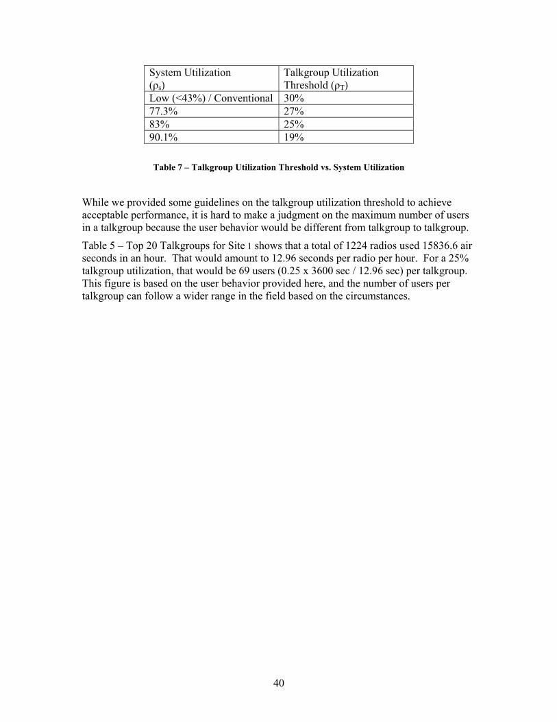
In this formula α is the benchmark for the talkgroup performance in a conventional system (or no waiting in central queue), and W(ρs) 31 is the average waiting time for all calls in the central queue, which is a function of the system utilization (ρs). This formula renders the appropriate talkgroup utilization at any system utilization, as long as the average waiting time in the central queue for that system utilization is known. For the example of 90.1% system utilization, where the average waiting time in the system under study was 1.674 seconds, and assuming the 30% benchmark (α=0.3), the talkgroup utilization should not exceed 19%. Using this formula, Table 7 tabulates the talkgroup utilization threshold for the cases we considered for the system under study.

30 See Appendix A for detailed derivation. 31 The average waiting time in the central queue can be obtained either directly through measured data, or through model calculations.

40

System Utilization (ρs)

Talkgroup Utilization Threshold (ρT)

Low (<43%) / Conventional 30% 77.3% 27% 83% 25% 90.1% 19%

Table 7 – Talkgroup Utilization Threshold vs. System Utilization

While we provided some guidelines on the talkgroup utilization threshold to achieve acceptable performance, it is hard to make a judgment on the maximum number of users in a talkgroup because the user behavior would be different from talkgroup to talkgroup.

Table 5 – Top 20 Talkgroups for Site 1 shows that a total of 1224 radios used 15836.6 air seconds in an hour. That would amount to 12.96 seconds per radio per hour. For a 25% talkgroup utilization, that would be 69 users (0.25 x 3600 sec / 12.96 sec) per talkgroup. This figure is based on the user behavior provided here, and the number of users per talkgroup can follow a wider range in the field based on the circumstances.

41

7. Potential Applications of Commercial Wireless Broadband Technologies

Our analysis of the Minneapolis bridge collapse allowed us to gauge the potential capabilities of future 4G broadband technologies to supplement or augment the capacity of existing public safety systems. 4G is a term used to describe the next evolution in wireless communications technology. This technology is expected to provide a broadband, IP-based network supporting voice, data and video services. 4G is composed of a number of foundational technologies including Multiple Input/Multiple Output (MIMO), Orthogonal Frequency Division Multiplexing (OFDM) and Advanced Channel Coding Techniques. All of these technologies were considered in our analysis. The performance differences between Worldwide Interoperability for Microwave Access (WiMAX) and Long Term Evolution (LTE) are not a dominant factor in the analysis because both are based on the core technologies listed above. WiMAX,32 which is the 4G technology modeled in our analysis, is based upon the IEEE 802.16 standard for fixed and mobile wireless connectivity. WiMAX is used herein as a surrogate for any of the leading 4G candidates such as LTE, an alternative 4G technology widely supported by the cellular industry.

The Minneapolis LMR system performed well during the bridge collapse and handled approximately twice the busy hour traffic. However, some sites were approaching saturation levels and not all public safety agencies can economically provide the same amount of surge capacity as Minneapolis. Thus, by conducting this study, we attempted to estimate the capacity of a hypothetical 4G broadband network, which may be used by public safety in the future to supplement or augment existing emergency communications systems.

7.1. Approach For this study, we chose typical WiMAX settings, along with 10 MHz of bandwidth, which is the same amount of bandwidth that was allocated for public safety broadband use in the 700 MHz band. We chose to model this by assuming that the 10 MHz of spectrum is allocated for public safety use only. Furthermore, we provided our estimates based on a mixture of voice and video traffic. To do so, we performed a two-step analysis. First, we made a baseline estimate of capacity. Second, as traffic was added, we compared this estimate with the performance of a simulated WiMAX node.33 For the simulation, we placed the hypothetical WiMAX base station at a location collocated with other existing tower structures that were located approximately 2.5

32 CSAD chose WIMAX due to its availability as a model in our simulation package. 33 See Appendix B for an explanation of baseline calculations.

42

kilometers from the I-35 Bridge and ensured that all handsets were within 3 kilometers of the base station. In a typical WiMAX deployment, the base station to base station spacing is 3 to 10 kilometers.34 Thus, the majority of handsets were placed at or near the bridge, as displayed in Figure 25, the WiMAX Network Diagram.

7.2. Modeling the 4G Broadband WiMAX network CSAD simulated a 4G broadband wireless system’s capacity with OPNET WiMAX Modeler 14.5.35 The OPNET Modeler is a discrete-event simulation tool with graphical user interface (GUI). The performance projections that we presented in this section were based on simulations with typical WiMAX Model attributes, network architecture, and equipment parameters listed in Table 8. However, it is important to note that local propagation conditions, configuration, and hardware choices may cause actual performance to differ. The advanced WiMAX systems will allow operators to modify their systems for a variety of unique services. For example, voice services require low latency and jitter unlike bandwidth-hungry data and streaming media applications. Because 4G technology tightly controls latency and jitter on links used for voice, while appropriately adjusting for various other types of data, 4G technology has the ability to deliver both voice and data services on the same network infrastructure. On the downlink, the base station directly controls the scheduling of traffic and the allocation of network resources. By dedicating a portion of the channel bandwidth, the operator can keep track of the allocated resources and transport any available packets from the appropriately classified traffic. On the uplink, there are several scheduling methods available to the operator, depending upon the Quality of Service (QoS) requirements for the service flow.36 WiMAX implements multiple QoS profiles to support multiple types of traffic. For example, each application and customer type can support a different set of requirements. In WiMAX networks, Unsolicited Grant Services (UGS) are designed to support fixed-size data packets at a constant bit rate (CBR). T1/E1 emulation, constant bit-rate, and VoIP services are all examples of applications that may use this service. Maximum sustained traffic rate, maximum latency, tolerated jitter, and request/transmission policies are all mandatory service flow parameters that define this service. Extended real-time Packet Service (ErtPS) is another service designed to support real-time applications, such as VoIP with silence suppression and Streaming Audio and Video applications that have variable data rates, but require guaranteed data rate and delay. This analysis also used UGS and ErtPS QoS profiles, due to their ability to support quality voice services. However, some QoS types that have been implemented within WIMAX will not support quality voice services, but will support data and other applications. Due to the complexities of estimating the realistic traffic loads for these QoS profiles, we did not consider these services for this report. 34 See WiMAX Forum, White Paper, 2nd Mobile Plugfest – Malaga, Spain,(February 2007). 35 See OPNET, available at www.opnet.com (last visited July 3, 2008). 36 See SR Telecom Inc., White Paper, WiMAX Capacity.

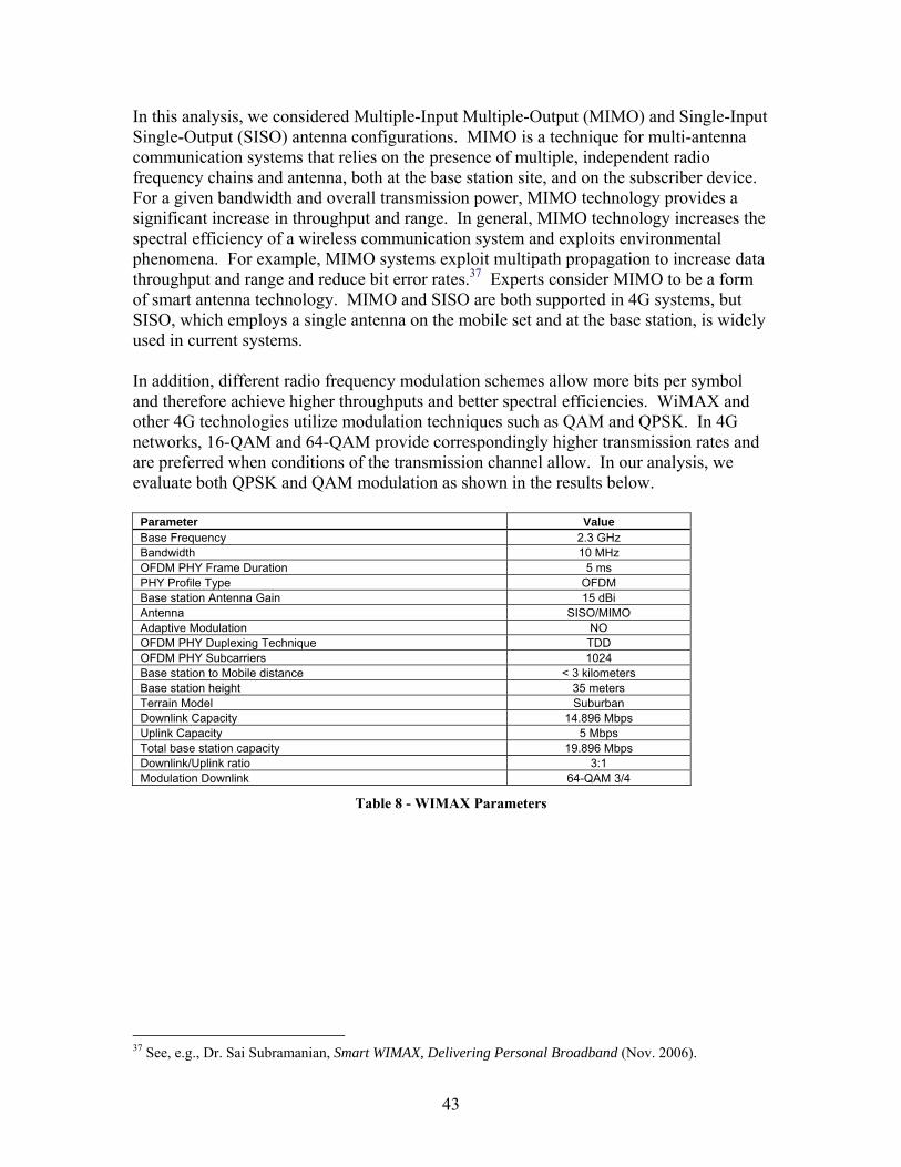
43

In this analysis, we considered Multiple-Input Multiple-Output (MIMO) and Single-Input Single-Output (SISO) antenna configurations. MIMO is a technique for multi-antenna communication systems that relies on the presence of multiple, independent radio frequency chains and antenna, both at the base station site, and on the subscriber device. For a given bandwidth and overall transmission power, MIMO technology provides a significant increase in throughput and range. In general, MIMO technology increases the spectral efficiency of a wireless communication system and exploits environmental phenomena. For example, MIMO systems exploit multipath propagation to increase data throughput and range and reduce bit error rates.37 Experts consider MIMO to be a form of smart antenna technology. MIMO and SISO are both supported in 4G systems, but SISO, which employs a single antenna on the mobile set and at the base station, is widely used in current systems. In addition, different radio frequency modulation schemes allow more bits per symbol and therefore achieve higher throughputs and better spectral efficiencies. WiMAX and other 4G technologies utilize modulation techniques such as QAM and QPSK. In 4G networks, 16-QAM and 64-QAM provide correspondingly higher transmission rates and are preferred when conditions of the transmission channel allow. In our analysis, we evaluate both QPSK and QAM modulation as shown in the results below.

Parameter Value Base Frequency 2.3 GHz Bandwidth 10 MHz OFDM PHY Frame Duration 5 ms PHY Profile Type OFDM Base station Antenna Gain 15 dBi Antenna SISO/MIMO Adaptive Modulation NO OFDM PHY Duplexing Technique TDD OFDM PHY Subcarriers 1024 Base station to Mobile distance < 3 kilometers Base station height 35 meters Terrain Model Suburban Downlink Capacity 14.896 Mbps Uplink Capacity 5 Mbps Total base station capacity 19.896 Mbps Downlink/Uplink ratio 3:1 Modulation Downlink 64-QAM 3/4

Table 8 - WIMAX Parameters

37 See, e.g., Dr. Sai Subramanian, Smart WIMAX, Delivering Personal Broadband (Nov. 2006).

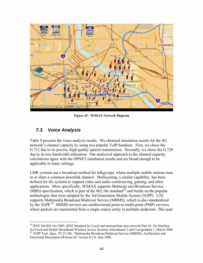
44

Figure 25 - WiMAX Network Diagram

7.3. Voice Analysis Table 9 presents the voice analysis results. We obtained simulation results for the 4G network’s channel capacity by using two popular VoIP handsets. First, we chose the G.711 due to its precise, high quality speech transmission. Secondly, we chose the G.729 due to its low bandwidth utilization. Our analytical approach to the channel capacity calculations agree with the OPNET simulation results and are broad enough to be applicable in many settings. LMR systems use a broadcast method for talkgroups, where multiple mobile stations tune to or share a common downlink channel. Multicasting, a similar capability, has been defined for 4G systems to support video and audio conferencing, gaming, and other applications. More specifically, WiMAX supports Multicast and Broadcast Service (MBS) specification, which is part of the 802.16e standard38 and builds on the popular technologies that were adopted by the 3rd Generation Mobile System (3GPP). LTE supports Multimedia Broadcast/Multicast Service (MBMS), which is also standardized by the 3GPP.39 MBMS services are unidirectional point-to-multi-point (PMP) services, where packets are transmitted from a single source entity to multiple endpoints. This type

38 IEEE Std 802.16e-2005, IEEE Standard for Local and metropolitan area network Part 16: Air Interface for Fixed and Mobile Broadband Wireless Access Systems Amendment 2 and Corrigendum 1, March 2008 39 3GPP Tech. Spec. TS 23.246, “Multimedia Broadcast/Multicast Service (MBMS); Architecture and Functional Description (Release 8)” version 8.2.0, June 2008.

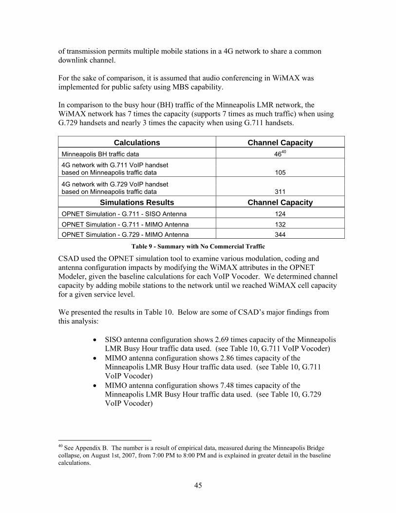
45

of transmission permits multiple mobile stations in a 4G network to share a common downlink channel. For the sake of comparison, it is assumed that audio conferencing in WiMAX was implemented for public safety using MBS capability. In comparison to the busy hour (BH) traffic of the Minneapolis LMR network, the WiMAX network has 7 times the capacity (supports 7 times as much traffic) when using G.729 handsets and nearly 3 times the capacity when using G.711 handsets.

Calculations Channel Capacity Minneapolis BH traffic data 4640

4G network with G.711 VoIP handset based on Minneapolis traffic data 105

4G network with G.729 VoIP handset based on Minneapolis traffic data 311

Simulations Results Channel Capacity OPNET Simulation - G.711 - SISO Antenna 124 OPNET Simulation - G.711 - MIMO Antenna 132 OPNET Simulation - G.729 - MIMO Antenna 344

Table 9 - Summary with No Commercial Traffic

CSAD used the OPNET simulation tool to examine various modulation, coding and antenna configuration impacts by modifying the WiMAX attributes in the OPNET Modeler, given the baseline calculations for each VoIP Vocoder. We determined channel capacity by adding mobile stations to the network until we reached WiMAX cell capacity for a given service level. We presented the results in Table 10. Below are some of CSAD’s major findings from this analysis:

• SISO antenna configuration shows 2.69 times capacity of the Minneapolis LMR Busy Hour traffic data used. (see Table 10, G.711 VoIP Vocoder)

• MIMO antenna configuration shows 2.86 times capacity of the Minneapolis LMR Busy Hour traffic data used. (see Table 10, G.711 VoIP Vocoder)

• MIMO antenna configuration shows 7.48 times capacity of the Minneapolis LMR Busy Hour traffic data used. (see Table 10, G.729 VoIP Vocoder)

40 See Appendix B. The number is a result of empirical data, measured during the Minneapolis Bridge collapse, on August 1st, 2007, from 7:00 PM to 8:00 PM and is explained in greater detail in the baseline calculations.

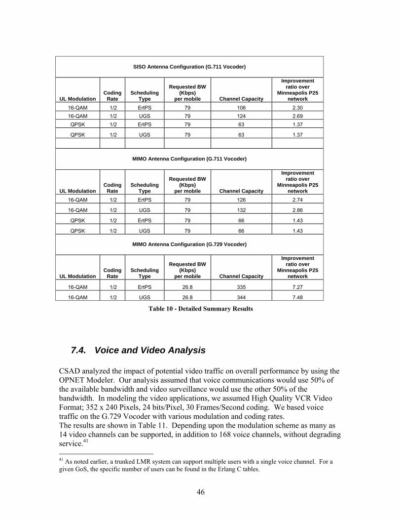
46

SISO Antenna Configuration (G.711 Vocoder)

UL Modulation Coding

Rate Scheduling

Type

Requested BW (Kbps)

per mobile Channel Capacity

Improvement ratio over

Minneapolis P25 network

16-QAM 1/2 ErtPS 79 106 2.30 16-QAM 1/2 UGS 79 124 2.69 QPSK 1/2 ErtPS 79 63 1.37

QPSK 1/2 UGS 79 63 1.37

MIMO Antenna Configuration (G.711 Vocoder)

UL Modulation Coding

Rate Scheduling

Type

Requested BW (Kbps)

per mobile Channel Capacity

Improvement ratio over

Minneapolis P25 network

16-QAM 1/2 ErtPS 79 126 2.74

16-QAM 1/2 UGS 79 132 2.86

QPSK 1/2 ErtPS 79 66 1.43

QPSK 1/2 UGS 79 66 1.43

MIMO Antenna Configuration (G.729 Vocoder)

UL Modulation Coding

Rate Scheduling

Type

Requested BW (Kbps)

per mobile Channel Capacity

Improvement ratio over

Minneapolis P25 network

16-QAM 1/2 ErtPS 26.8 335 7.27

16-QAM 1/2 UGS 26.8 344 7.48

Table 10 - Detailed Summary Results

7.4. Voice and Video Analysis

CSAD analyzed the impact of potential video traffic on overall performance by using the OPNET Modeler. Our analysis assumed that voice communications would use 50% of the available bandwidth and video surveillance would use the other 50% of the bandwidth. In modeling the video applications, we assumed High Quality VCR Video Format; 352 x 240 Pixels, 24 bits/Pixel, 30 Frames/Second coding. We based voice traffic on the G.729 Vocoder with various modulation and coding rates. The results are shown in Table 11. Depending upon the modulation scheme as many as 14 video channels can be supported, in addition to 168 voice channels, without degrading service.41 41 As noted earlier, a trunked LMR system can support multiple users with a single voice channel. For a given GoS, the specific number of users can be found in the Erlang C tables.

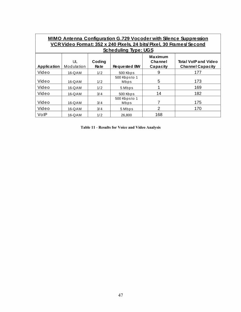
47

MIMO Antenna Configuration G.729 Vocoder with Silence Suppression VCR Video Format: 352 x 240 Pixels, 24 bits/Pixel, 30 Frames/Second

Scheduling Type: UGS

Application UL

Modulation Coding

Rate Requested BW

Maximum Channel Capacity

Total VoIP and Video Channel Capacity

Video 16-QAM 1/2 500 Kbps 9 177

Video 16-QAM 1/2 500 Kbps to 1

Mbps 5 173 Video 16-QAM 1/2 5 Mbps 1 169 Video 16-QAM 3/4 500 Kbps 14 182

Video 16-QAM 3/4 500 Kbps to 1

Mbps 7 175 Video 16-QAM 3/4 5 Mbps 2 170 VoIP 16-QAM 1/2 26,800 168

Table 11 - Results for Voice and Video Analysis

48

8. Conclusions In this analysis, CSAD obtained empirical data from the emergency communication system that was used by the public safety community to respond to the Minneapolis bridge collapse. First, CSAD used the data to calibrate a computer model of the communications system. Second, CSAD extended its analysis to other operating environments. Finally, CSAD evaluated the impact of next generation commercial mobile systems on emergency communications in similar environments. By comparing the voice traffic profiles that arose before and during the disaster, CSAD illustrated the unique nature of emergency communications: relatively short calls of approximately six seconds in duration, coupled with the use of large conferencing capabilities, otherwise known as talkgroups. Our analysis also revealed that certain elements of the Minneapolis communication system were beginning to approach their maximum effective capacity. CSAD also developed a computer simulation which demonstrated that the actual system conformed well to common traffic models. Notably, our simulation can be used by the public safety community to calculate the communications resource requirements that will be necessary to achieve their defined performance goals. For example, CSAD provided the performance bounds for the studied system. A public safety entity can also apply traffic characterizations from this study to analyze scenarios that were not presented by the Minneapolis disaster. CSAD also analyzed the impact of a hypothetical 4G broadband wireless communications systems on emergency communications at the site. 4G technologies are expected to be available over the next few years and will have operational characteristics that will allow them to supplement or augment emergency communication systems. CSAD found that a single 4G cell site within the downtown Minneapolis area would have provided several times the capacity of the embedded emergency communications systems.

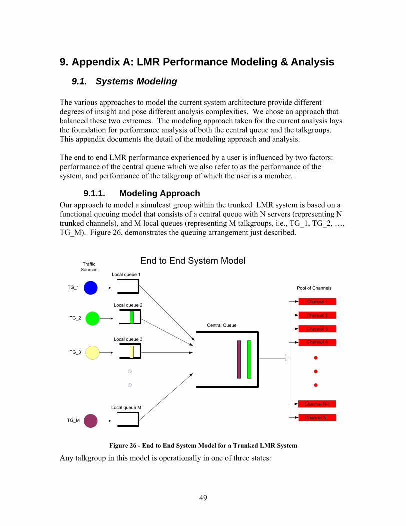
49

9. Appendix A: LMR Performance Modeling & Analysis

9.1. Systems Modeling The various approaches to model the current system architecture provide different degrees of insight and pose different analysis complexities. We chose an approach that balanced these two extremes. The modeling approach taken for the current analysis lays the foundation for performance analysis of both the central queue and the talkgroups. This appendix documents the detail of the modeling approach and analysis. The end to end LMR performance experienced by a user is influenced by two factors: performance of the central queue which we also refer to as the performance of the system, and performance of the talkgroup of which the user is a member.

9.1.1. Modeling Approach Our approach to model a simulcast group within the trunked LMR system is based on a functional queuing model that consists of a central queue with N servers (representing N trunked channels), and M local queues (representing M talkgroups, i.e., TG_1, TG_2, …, TG_M). Figure 26, demonstrates the queuing arrangement just described.

TG_1

Local queue 1

TG_3

Local queue 3

TG_M

Local queue M

TG_2

Local queue 2Channel 1

Channel N

Channel N-1

Channel 4

Channel 3

Channel 2

Central Queue

Traffic Sources

End to End System Model

Pool of Channels

Figure 26 - End to End System Model for a Trunked LMR System

Any talkgroup in this model is operationally in one of three states:

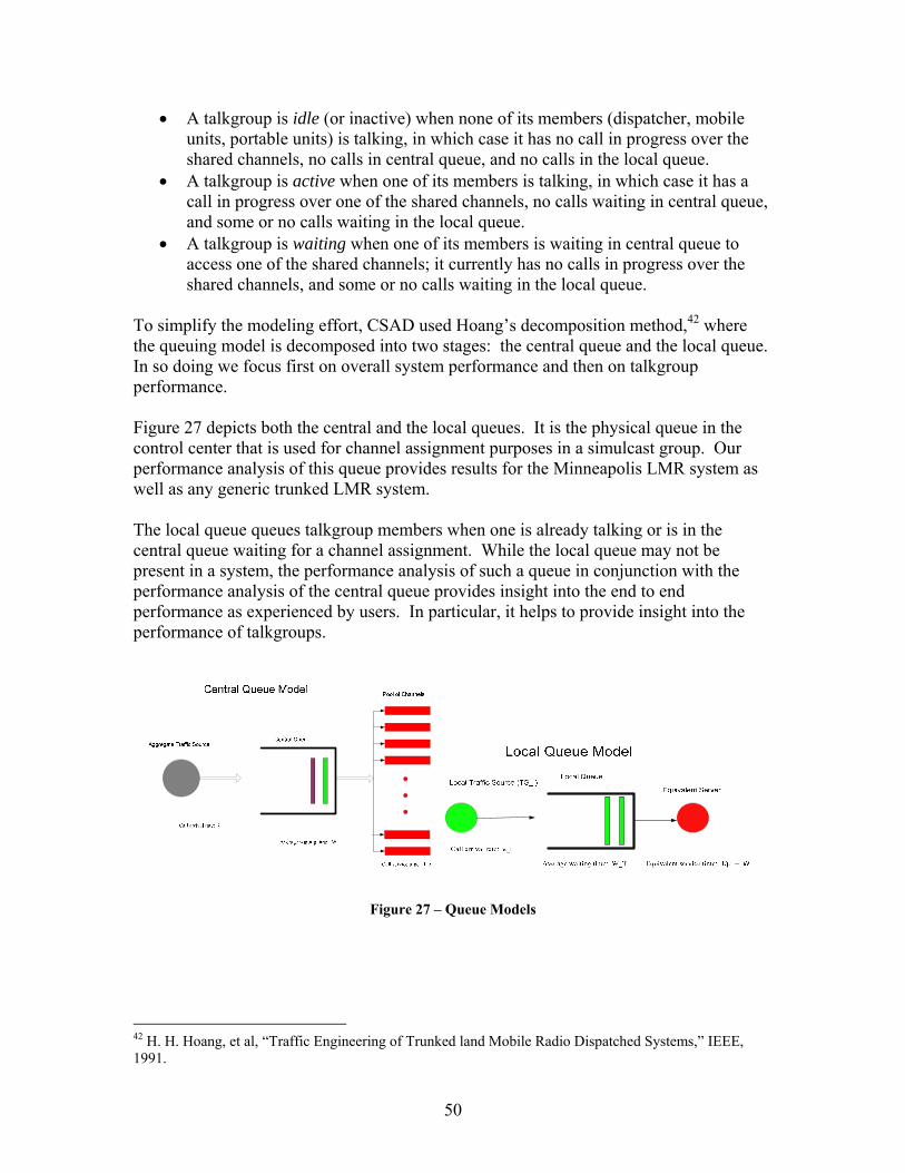
50

• A talkgroup is idle (or inactive) when none of its members (dispatcher, mobile units, portable units) is talking, in which case it has no call in progress over the shared channels, no calls in central queue, and no calls in the local queue.

• A talkgroup is active when one of its members is talking, in which case it has a call in progress over one of the shared channels, no calls waiting in central queue, and some or no calls waiting in the local queue.

• A talkgroup is waiting when one of its members is waiting in central queue to access one of the shared channels; it currently has no calls in progress over the shared channels, and some or no calls waiting in the local queue.

To simplify the modeling effort, CSAD used Hoang’s decomposition method,42 where the queuing model is decomposed into two stages: the central queue and the local queue. In so doing we focus first on overall system performance and then on talkgroup performance. Figure 27 depicts both the central and the local queues. It is the physical queue in the control center that is used for channel assignment purposes in a simulcast group. Our performance analysis of this queue provides results for the Minneapolis LMR system as well as any generic trunked LMR system. The local queue queues talkgroup members when one is already talking or is in the central queue waiting for a channel assignment. While the local queue may not be present in a system, the performance analysis of such a queue in conjunction with the performance analysis of the central queue provides insight into the end to end performance as experienced by users. In particular, it helps to provide insight into the performance of talkgroups.

Figure 27 – Queue Models

42 H. H. Hoang, et al, “Traffic Engineering of Trunked land Mobile Radio Dispatched Systems,” IEEE, 1991.

51

9.1.2. System Parameters and Performance Metrics

• Central Queue The central queue, which follows an Erlang C model, is a multi server queue with N servers (channels), and a “First-In-First-Out” (FIFO) discipline. This queuing model assumes the aggregate traffic arrival from all the sites within a simulcast group to exhibit statistics consistent with a Poisson probability distribution with a mean rate of λ calls/sec. It follows that the call interarrival time is exponentially distributed with a mean of 1/λ.43 Call duration is also exponentially distributed with a mean of 1/µ seconds. The total offered traffic load is defined to be A= λ/µ erlang. The system utilization is defined to be ρ= λ/(Nµ), which should be less than one to ensure system stability. We calibrated our model using data from the Minneapolis disaster by calculating the statistical mean of call interarrival and call duration from the empirical data. Calibration ensures that the fundamental parameters of the model are pegged to real, observed data and gives us confidence that the parameters can be altered to predict system performance under different conditions.

Performance Metrics

Most system performance metrics are based on the statistics obtained for the central queue. These include waiting probability (probability of a call waiting in the queue to grab a channel), PW, and average waiting time (or queuing delay) for those calls that have to wait in the central queue, WC. The waiting probability, PW is the probability that a call upon its arrival has to wait in the central queue for channel access. Average waiting time (WC), otherwise known as queuing delay, is the average waiting time for those calls that have to wait in the central queue before being assigned a channel. This is different than the average waiting time for all calls, which includes those that do not have to wait in the queue. WC is equal to the waiting time for all calls divided by the waiting probability, PW. The performance metrics introduced here are used to define the Grade of Service (GoS) for LMR systems. GoS uses performance metrics and sets objective thresholds for them. An example of such GoS here is the percentage of calls that experience queuing delays beyond certain threshold. For instance, we can choose 2% of calls that experience a wait time of 3 seconds or more as a benchmark for design. Mathematically, this translates to the probability of W≥3 seconds being 0.02, which is obtained from the statistics of W that are embedded in our system model.

43 Queuing Syste ms, Volume 1: Theory, Leonard Kleinrock, 1975.

52

In this report we also discuss system design and capacity considerations for a trunked LMR system. We determine, based on a predefined GoS, the allowable region of operation, i.e., the required number of channels (or spectrum) versus system utilization. Similarly, we determine, based on a predefined GoS, the capacity regions, i.e., the required number of channels (or spectrum) versus traffic intensity (erlang).

• Local Queue We use the well known M/M/1 queuing model44 to represent the local queue. The local queue is a one channel queue with “First-In-First-Out” (FIFO) traffic discipline; hence the call interarrival and call durations are both exponentially distributed. The average call arrival rate is assumed to be λ1 calls per second. The average call duration is assumed to be 1/µ sec. As part of the decomposition approach explained earlier, the performance impact of the central queue is considered in order to calculate the performance of local queue. Specifically, the equivalent service time45 for the local queue is equal to the call duration plus the average waiting time incurred by all calls in the central queue. If we assume the equivalent service time for the local queue to be 1/µg,,then 1/µg = 1/µ + W where W, the average waiting time for all calls in the central queue, is obtained from the calculations of central queue. The total offered traffic load to the local queue is defined to be A= λ1/µ erlang. The talkgroup utilization, which is different than the system utilization defined earlier, is also defined to be ρ= λ1/µ. However, the local queue utilization is λ1/µg which should be less than one for stability of the queue.46 Performance Metrics Though many performance metrics can be considered for local queue, we are interested in metrics such as total time spent in the system, waiting time in the local queue, and total waiting time in both queues. Total time spent in the system which includes waiting time in local queue, waiting time in central queue, and call duration, is calculated from 1/(µg- λ1). Waiting time in the local queue is calculated from 1/(µg- λ1) - 1/µg. Total waiting time in both queues (queuing delay) is calculated from 1/(µg- λ1) - 1/µ. For trunked LMR systems, the average delay experienced by the end-user is equivalent to the sum of the delay in the local and central queues. For LMR systems, which do not have local queues, local queue performance is merely a surrogate for the user perceived performance in accessing the channel. We use the waiting time in the local queue to derive talkgroup utilization thresholds for acceptable performance for talkgroups.

44 Queuing Systems, Volume 1: Theory, Leonard Kleinrock, 1975. 45 In queuing terminology, service time is defined as the time that a customer receives service. In regard to this case study, the equivalent service time is equal to call duration when there is no queuing delay in the central queue. 46 This formula translates to ρ< 1/(1+µW).

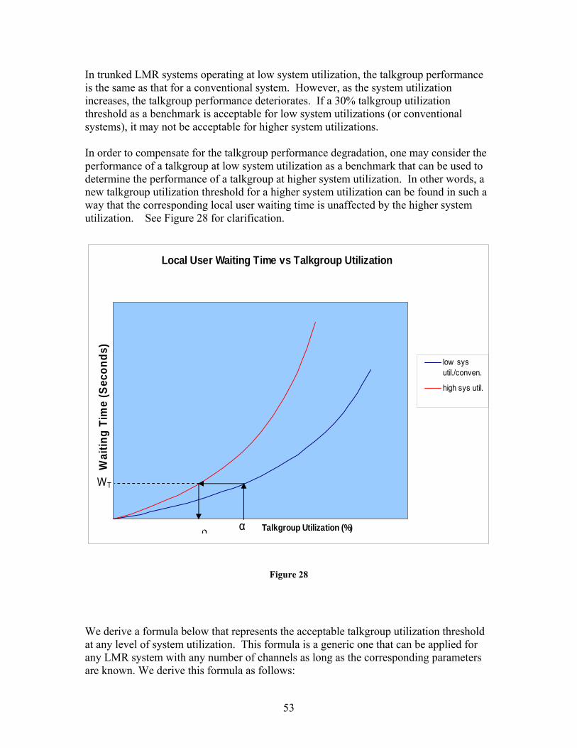
53

In trunked LMR systems operating at low system utilization, the talkgroup performance is the same as that for a conventional system. However, as the system utilization increases, the talkgroup performance deteriorates. If a 30% talkgroup utilization threshold as a benchmark is acceptable for low system utilizations (or conventional systems), it may not be acceptable for higher system utilizations. In order to compensate for the talkgroup performance degradation, one may consider the performance of a talkgroup at low system utilization as a benchmark that can be used to determine the performance of a talkgroup at higher system utilization. In other words, a new talkgroup utilization threshold for a higher system utilization can be found in such a way that the corresponding local user waiting time is unaffected by the higher system utilization. See Figure 28 for clarification.

Figure 28

We derive a formula below that represents the acceptable talkgroup utilization threshold at any level of system utilization. This formula is a generic one that can be applied for any LMR system with any number of channels as long as the corresponding parameters are known. We derive this formula as follows:

Local User Waiting Time vs Talkgroup Utilization

Talkgroup Utilization (%)

Wai

ting

Tim

e (S

econ

ds)

low sysutil./conven.

high sys util.

α

WT

ρ

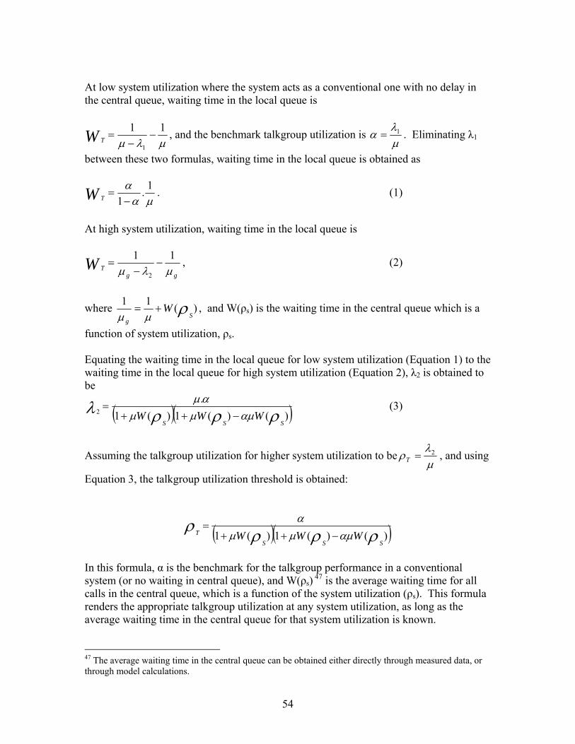
54

At low system utilization where the system acts as a conventional one with no delay in the central queue, waiting time in the local queue is

µλµ11

1

−−

=W T, and the benchmark talkgroup utilization is

µλ

α 1= . Eliminating λ1

between these two formulas, waiting time in the local queue is obtained as

µαα 1.

1−=W T . (1)

At high system utilization, waiting time in the local queue is

ggTW µλµ

11

2

−−

= , (2)

where )(11 ρµµ Sg

W+= , and W(ρs) is the waiting time in the central queue which is a

function of system utilization, ρs. Equating the waiting time in the local queue for low system utilization (Equation 1) to the waiting time in the local queue for high system utilization (Equation 2), λ2 is obtained to be

( )( ))()(1)(1.

2 ρρρλ αµµµαµ

SSSWWW −++

= (3)

Assuming the talkgroup utilization for higher system utilization to beµλ

ρ 2=T , and using

Equation 3, the talkgroup utilization threshold is obtained:

( )( ))()(1)(1 ρρρραµµµ

α

SSST WWW −++=

In this formula, α is the benchmark for the talkgroup performance in a conventional system (or no waiting in central queue), and W(ρs) 47 is the average waiting time for all calls in the central queue, which is a function of the system utilization (ρs). This formula renders the appropriate talkgroup utilization at any system utilization, as long as the average waiting time in the central queue for that system utilization is known.

47 The average waiting time in the central queue can be obtained either directly through measured data, or through model calculations.

55

9.2. Prior Work for LMR Performance Analysis by Others The Analytical work to evaluate the performance of conventional and then trunked LMR systems go back to the 1980s. The work in this area is limited in quantity. In the early 1990’s, there has been some work to model the end to end trunked LMR system, and in particular, Hoang et al,48 introduced a system model that models a central queue preceded by a group of queues representing the fleets (or talkgroups). Then they proposed an analytical approach, namely decomposition method to solve the problem.49 They applied this method to provide analytical solutions to provide performance metrics of the trunked LMR dispatch systems. They also used simulation tools to prove their approach. Recently, in 2004-2006, a group of university researchers at Simon Fraser University (Vancouver, British Columbia, Canada) addressed the performance of an LMR system using the empirical data collected from a deployed system in the south western British Columbia, very similar to the current system under study. They did extensive studies on the nature and pattern of traffic,50 and did some simulations as well.51 They made assessments, in particular, on the call interarrival and call duration patterns. They claimed that the call interarrival is best modeled by an exponential distribution while the call duration is best modeled by a Lognormal distribution.52 Later on, they claimed that the call interarrival is best modeled by both Weibull and Gamma distributions, and maintained that the call duration is best modeled by a Lognormal distribution.53 It is worth noting that exponential distribution is a special form of Gamma distribution (with parameters α (shape) and β (scale)) where its shaping factor is equal to 1. In the wake of studies in the past, we decided to do some brief research of our own, in order to decide what we should choose for our system modeling parameters. We developed a simulation model on a part of the system (Central Queue), which is a multiserver queue with FIFO discipline. We set the call interarrivals to follow a Gamma distribution and the call durations follow a Lognormal distribution. We used the empirical data for the parameters of the distributions. We also, in another scenario, set both distributions to be exponential with appropriate empirical parameters. We ran the simulations and tabulated the results in Table 12 and Table 13. We concluded that both scenarios performed almost the same, and the results were very close to the practical 48 H. H. Hoang, et al, “Traffic Engineering of Trunked land Mobile Radio Dispatched Systems”, IEEE, 1991. 49 H. H. Hoang et al, ”Communication Load and Delay in Multichannel Land Mobile Systems for Dispatch Traffic: a Queuing Model Analysis”, IEEE, 1992. 50 N. Cackov, B. Vujičić, S. Vujičić, and Lj. Trajković, “Using Network Activity Data to Model the Utilization of a Trunked Radio System,” Proc. SPECTS, San Jose, CA, July 2004, pp. 517– 524. 51 N. Cackov, J. Song, B. Vujicic, S. Vujicic, and Lj. Trajkovic, “Simulation and Performance Evaluation of a Public Safety Wireless Network: Case Study,'' Simulation, vol. 81, no. 8, pp. 571–585, Aug. 2005. 52 D. Sharp, N. Cackov, N. Lasković, Q. Shao, and Lj. Trajković, “Analysis of Public Safety Traffic on Trunked Land Mobile Radio Systems,” IEEE J. Select. Areas Commun., vol. 22, no. 7, pp. 1197–1205, Sept. 2004. 53 B. Vujičić, N. Cackov, S. Vujičić, and Lj. Trajković, “Modeling and Characterization of Traffic in Public Safety Wireless Networks,” in Proc. SPECTS 2005, Philadelphia, PA, July 2005, pp. 14–223.

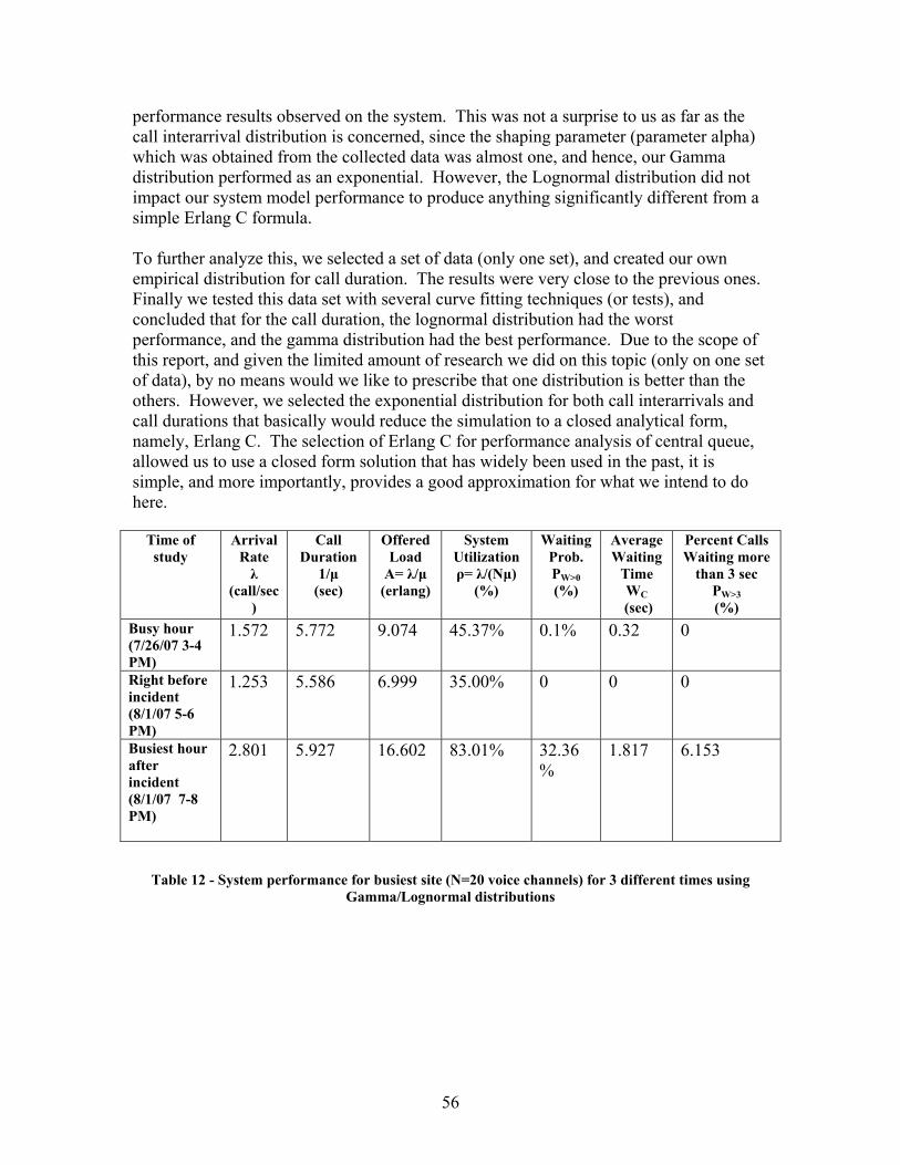
56

performance results observed on the system. This was not a surprise to us as far as the call interarrival distribution is concerned, since the shaping parameter (parameter alpha) which was obtained from the collected data was almost one, and hence, our Gamma distribution performed as an exponential. However, the Lognormal distribution did not impact our system model performance to produce anything significantly different from a simple Erlang C formula. To further analyze this, we selected a set of data (only one set), and created our own empirical distribution for call duration. The results were very close to the previous ones. Finally we tested this data set with several curve fitting techniques (or tests), and concluded that for the call duration, the lognormal distribution had the worst performance, and the gamma distribution had the best performance. Due to the scope of this report, and given the limited amount of research we did on this topic (only on one set of data), by no means would we like to prescribe that one distribution is better than the others. However, we selected the exponential distribution for both call interarrivals and call durations that basically would reduce the simulation to a closed analytical form, namely, Erlang C. The selection of Erlang C for performance analysis of central queue, allowed us to use a closed form solution that has widely been used in the past, it is simple, and more importantly, provides a good approximation for what we intend to do here.

Table 12 - System performance for busiest site (N=20 voice channels) for 3 different times using

Gamma/Lognormal distributions

Time of study

Arrival Rate λ

(call/sec)

Call Duration

1/µ (sec)

Offered Load

A= λ/µ (erlang)

System Utilization ρ= λ/(Nµ)

(%)

Waiting Prob. PW>0 (%)

Average Waiting

Time WC

(sec)

Percent Calls Waiting more

than 3 sec PW>3 (%)

Busy hour (7/26/07 3-4 PM)

1.572 5.772 9.074 45.37% 0.1% 0.32 0

Right before incident (8/1/07 5-6 PM)

1.253 5.586 6.999 35.00% 0 0 0

Busiest hour after incident (8/1/07 7-8 PM)

2.801 5.927 16.602 83.01% 32.36%

1.817 6.153

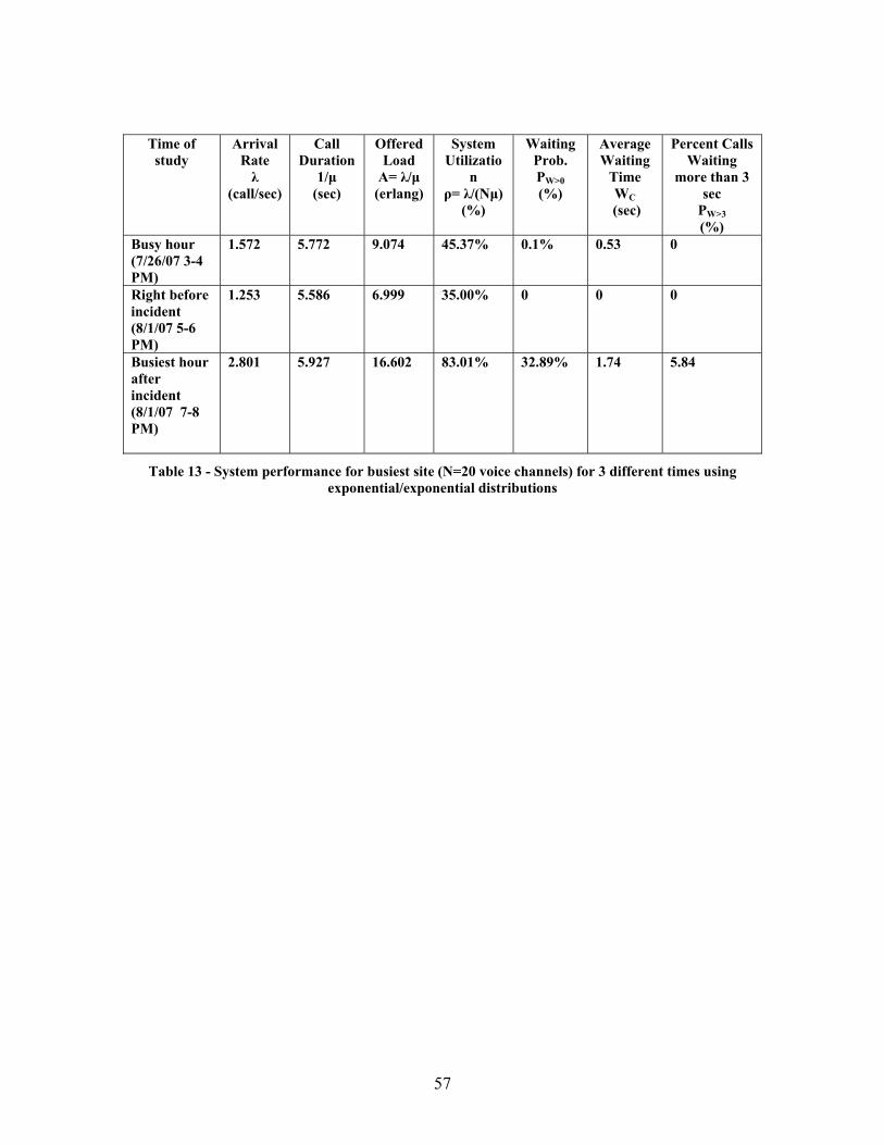
57

Table 13 - System performance for busiest site (N=20 voice channels) for 3 different times using exponential/exponential distributions

Time of study

Arrival Rate λ

(call/sec)

Call Duration

1/µ (sec)

Offered Load

A= λ/µ (erlang)

System Utilizatio

n ρ= λ/(Nµ)

(%)

Waiting Prob. PW>0 (%)

Average Waiting

Time WC

(sec)

Percent Calls Waiting

more than 3 sec

PW>3 (%)

Busy hour (7/26/07 3-4 PM)

1.572 5.772 9.074 45.37% 0.1% 0.53 0

Right before incident (8/1/07 5-6 PM)

1.253 5.586 6.999 35.00% 0 0 0

Busiest hour after incident (8/1/07 7-8 PM)

2.801 5.927 16.602 83.01% 32.89% 1.74 5.84

58

10. Appendix B: Baseline calculation of Voice over IP (VoIP)

The Minneapolis public safety users have P25 mobile voice radios with 4.4 Kbps Improved Multi-Band Excitation (IMBE) Vocoder, with 2.8 Kbps Error Correction Coding and 2.4 Kbps Embedded Signaling. This is a total signaling Rate of 9.6 Kbps. The voice IMBE Vocoder is intended to be used throughout Project 25 in any equipment that requires an analog-to-digital or digital-to-analog voice interface. Since no comparable VoIP Vocoder matches the technical characteristics and signaling rates of the P25 IMBE Vocoder mentioned above, the G.711 (64 Kbps) and G.729 (8 Kbps) VoIP Vocoder were chosen for this analysis. The G.711 codec yields the same voice quality as the public network, but requires more bandwidth because of the IP overhead added to each packet. The G.729 codec uses less bandwidth comparable to the P25 IMBE, but the voice quality is lower. Voice clarity with the G.711 is on par with the public switched telephone network (PSTN). G.711 will provide toll quality even when used in off-network applications to PSTN phones. Voice quality with the G.729 is less assured. Although G.729 requires significantly less bandwidth than the G.711, it does not provide toll quality speech in practice.54 The G.711 and G.729 are also supported by VOIP providers and the 4G WiMAX technology. Given;

• Codec G.711 – 64 kbps rate, 20 ms sample period, used with compressed RTP headers and UDP checksums, one packet is sent every 20 ms, 50 packets per second.

• Payload is 64,000 ÷ 50 = 1,280 bits. • Overhead which includes IP, UDP or link headers = 300 bits. • Total size is 1,580 bits.

Then: • Average VoIP Bandwidth required is (1,580) x 50 = 79 Kbps.

Silence Suppression or Voice Activity Detection (VAD) suppresses the transmission of data during silence periods. As only one person normally speaks at a time, this can reduce the demand for bandwidth by as much as 50 percent.55 With circuit-switched voice networks, all voice calls use 64 Kbps fixed-bandwidth links regardless of how much of the conversation is speech and how much is silence. With VOIP networks, all conversation and silence is packetized. Using VAD, packets of silence can be suppressed.56 In our calculation for silence suppression, we use a VAD factor of 40 percent bandwidth savings.

54 David A. Garbin, Voice Quality End to End, 2006. 55 Newport Networks Ltd , VoIP Bandwidth Calculation, 2005. 56 Cisco, “Cisco - Voice Over IP - Per Call Bandwidth Consumption,” 2005.

59

• Average VoIP Bandwidth (G.711 Vocoder) required with Silence Suppression = 47.4 Kbps

Given;

• Codec G.729 – 8 kbps rate, overhead and 50 packets per second. Then;

• Average VoIP Bandwidth (G.729 Vocoder) required is = 26.8 Kbps With Silence Suppression;

• Average VoIP Bandwidth (G.729 Vocoder) required with Silence Suppression is = 16.08 Kbps

Calculation of Channels required for each Vocoder In a 4G WiMAX network the Downlink (DL) to Uplink capacity ratio is typically 3:1; with the Uplink channel size for one cell site typically 5 Megabits per second (Mbps).57 Assuming the network is Uplink (UL) limited on bandwidth, then for a 5 Mbps UL capacity in a 4G WiMAX network and the above average bandwidth requirement, the total Channels required per cell would be;58

• Uplink 4G WiMAX network = 5 Mbps / 47.4 Kbps = 105 Channels per cell. (G.711 Vocoder)

• Uplink 4G WiMAX network = 5 Mbps / 16.08 Kbps = 311 Channels per cell. (G.729 Vocoder)

Calculation of Channels required with Minneapolis BH traffic data The total BH voice traffic during the Minneapolis Bridge collapse on August 1st, 2007 from 7 to 8 PM, for the two busiest sites was 30.7 Erlangs. The total traffic from two sites was used, for equivalency to the WiMAX base station to base station spacing. We used the actual traffic data to attain the BH total traffic which is the actual length of time the call was on the air, not including time spent in the busy queue. Traffic of one Erlang refers to a single resource being in continuous use, or two channels being at fifty percent use, and so on.59 For example, if an office had two telephone operators, two simultaneous users, who are both busy all the time, that would represent two Erlangs of traffic, or a radio channel that is occupied for thirty minutes during an hour is said to carry 0.5 Erlang of traffic. In turn, Channel Capacity, or an Erlang can be referenced as a simultaneous user, which occupies the continuous use of a traffic channel.

• Assuming 1% Grade of Service (GoS) the 30.7 Erlangs equates (using Erlang C traffic tables) to a requirement of 46 channels.

57 Loutfi Nuaymi, SIMPLE CAPACITY ESTIMATIONS IN WIMAX/802.16 SYSTEM, 2006 58 SR Telecom Inc., WiMAX Capacity, White Paper, (2006). 59 See Wikipedia, Erlang Unit, available at http://en.wikipedia.org/wiki/Erlang_unit (as of July 2008).

60

Capacity in a 4G WiMAX Network Assuming the rate is about 47.4 kbps from above, for a VOIP call counting all application headers overhead, then the total bandwidth required to support VOIP will therefore be:

• BW VoIP to support Minneapolis Bridge traffic = 46 Channels * 47.4 kbps = 2.1804 Mbps. (G.711 Vocoder)

• BW VoIP to support Minneapolis Bridge traffic = 46 channels * 16.08 kbps = 739.68 Kbps. (G.729 Vocoder)

Therefore, the capacity of a 4G WiMAX network compared to the Minneapolis P25 network, with the G.711 Vocoder is;

• 5 Mbps / 2.1804 Mbps = 2.29 times greater capacity in a 4G WiMAX network. With the G.729 Vocoder and bandwidth comparable to the P25 IMBE, the capacity is;

• 5 Mbps / 739.68 Kbps = 6.76 times greater capacity in a 4G WiMAX network. Therefore, the entire capacity of a 4G WiMAX network could theoretically support more than 6 times the equivalent demand of BH traffic during the Minneapolis Bridge collapse using equivalent 4G VOIP calls.

61