embedded vehicle dynamics aiding for usbl/ins underwater...

This article has been accepted for inclusion in a future issue of this journal. Content is final as presented, with the exception of pagination.

IEEE TRANSACTIONS ON CONTROL SYSTEMS TECHNOLOGY 1

Embedded Vehicle Dynamics Aiding for USBL/INS UnderwaterNavigation System

Marco Morgado, Paulo Oliveira, Carlos Silvestre, and José Fernandes Vasconcelos

Abstract— This brief presents an embedded vehicle dynamics(VD) aiding technique to enhance position, velocity, and attitudeerror estimation in low-cost inertial navigation systems (INSs),with application to underwater vehicles. The model of the VDprovides motion information that is complementary to the INSand, consequently, the fusion of both systems allows for acomprehensive improvement of the overall navigation systemperformance. In this brief, the specific VD equations of motionare directly embedded in an extended Kalman filter, as opposedto classical external vehicle models that act as secondary INSs.A tightly-coupled inverted ultrashort baseline is also adopted toenhance position and attitude estimation using measurementsof relative position of a transponder located in the vehiclemission area. The improvement of the overall navigation system isassessed in simulation using a nonlinear model of the INFANTEautonomous underwater vehicle, resorting to extensive MonteCarlo runs that implement perturbed versions of the nominaldynamics. The results show that the vehicle dynamics producerelevant performance enhancements, and that the accuracy ofthe system is robust to modeling uncertainties.

Index Terms— Inertial navigation systems, position andattitude estimation, ultrashort baseline, vehicle dynamics (VD)aiding.

NOMENCLATURE

Column vectors and matrices are denoted, respectively, byboldfaced lower-case and upper-case symbols, e.g., y andY. Scalar quantities are represented by lower-case regulartypeface symbols, e.g., y. The representation [y×] is the skew-symmetric matrix that denotes the cross product of y ∈ R

3

and u ∈ R3 such that [y × ]u = y × u. The transpose of

a vector or matrix will be indicated with the superscript T ,

Manuscript received April 18, 2011; revised December 12, 2012;accepted January 13, 2013. Manuscript received in final form Janu-ary 31, 2013. This work was supported in part by the FCT under GrantPEst-OE/EEI/LA0009/2011, and Project FCT PTDC/EEA-CRO/111197/2009—MAST/AM, and the EU Project TRIDENT under Contract 248497.The work of M. Morgado was supported by the Portuguese FCT POCTIProgramme, Ph.D. Student Scholarship, under Grant SFRH/BD/25368/2005.Recommended by Associate Editor A. Serrani.

M. Morgado and J. F. Vasconcelos are with the Laboratory of Robot-ics and Systems in Engineering and Science, Instituto Superior Técnico,Universidade Técnica de Lisboa, Lisbon 1049-001, Portugal (e-mail:[email protected]; [email protected]).

P. Oliveira is with the Department of Mechanical Engineering and with theLaboratory of Robotics and Systems in Engineering and Science, InstitutoSuperior Técnico, Universidade Técnica de Lisboa, Lisbon 1049-001, Portugal(e-mail: [email protected]).

C. Silvestre was with the Department of Electrical Engineering and Com-puters, and Laboratory of Robotics and Systems in Engineering and Science,Instituto Superior Técnico, Universidade Técnica de Lisboa, Lisbon 1049-001, Portugal. He is now with the Department of Electrical and ComputerEngineering, Faculty of Science and Technology, University of Macau, Macau100872, China (e-mail: [email protected]).

Color versions of one or more of the figures in this paper are availableonline at http://ieeexplore.ieee.org.

Digital Object Identifier 10.1109/TCST.2013.2245133

e.g., yT or YT . Leading subscripts and superscripts identifythe coordinate system of a quantity, e.g., E y is represented inthe earth-fixed coordinate frame and By is represented in thebody-fixed coordinate frame. The matrix R ∈ SO(3) is theshorthand notation for body {B} to earth {E} coordinate framesrotation matrix E

B R, that transforms the vector representationBy into E y by means of the linear operation E y = E

BRBy. Themeasurement and the estimate of quantity y are denoted byyr and y, respectively. The attitude error rotation vector δλ isdefined by R(δλ) � RRT . Position, velocity and accelerationare denoted, respectively, by p, v, and a, and the angularvelocity of the vehicle expressed in body-fixed coordinatesby ω. The position of a transponder in earth coordinates isdenoted by s, and the transponder position in body coordinateframe is represented by r. The superscripts + and − denotea priori information and corrected a posteriori quantities,respectively, e.g., s+ and s−.

I. INTRODUCTION

THE DESIGN and implementation of navigation systemsstands out as one of the most critical steps toward the

successful operation of autonomous vehicles. The quality ofposition, velocity, and attitude estimates of the navigationsystem dramatically influences the capability of the vehicles toperform precision-demanding tasks. See [1] for an interestingand detailed survey on underwater vehicle navigation and itsrelevance. Performance degradation and limitations inherent tolow-cost inertial navigation system (INSs), associated to open-loop unbounded estimation errors, unfiltered sensor noise, anduncompensated bias effects, are often tackled by merging addi-tional information sources with nonlinear filtering techniques.Among a diverse set of techniques, an extended Kalman filter(EKF) in a direct-feedback configuration [2] is commonlyadopted to estimate and compensate the INS integration errorbuildup. This brief addresses the merging of underwater VDinformation with a low-cost INS, by means of a reduced-stateinternal vehicle model, as opposed to classical fully-fledgedexternal vehicle models aiding techniques, and presents anexhaustive assessment of the achievable performance improve-ment.

Available underwater navigation aiding sensors includeDoppler velocity log (DVL), inclinometers, depth pressuresensors, magnetic compasses, whereas acoustic systems sys-tems [3], [4], such as long baseline (LBL), short baseline(SBL), and ultrashort baseline (USBL), often stand as the pri-mary choice for underwater positioning [5], [6]. Although longbaseline-based solutions offer more information and precision,key factors, such as high-cost and time-consuming procedures

1063–6536/$31.00 © 2013 IEEE


2 IEEE TRANSACTIONS ON CONTROL SYSTEMS TECHNOLOGY

for deployment and calibration, prohibit their use in low-costoperations. Hull-mounted short baseline positioning systems,in large oceanic vessels, have to actively compensate for base-line changes due to natural bending of the hull, degrading theirperformance. The fast deployment, less complex hardware, andincreasing performance of modern factory-calibrated ultrashortbaseline positioning devices makes them suitable for fasterdeployment intervention missions, when compared to longbaseline dependent solutions.

The development of the aforementioned navigation systemsstill has to bear in mind key features, such as low-cost,compactness, high performance, versatility, and robustness.The scientific community has been striving to improve low-cost navigation systems accuracy, directing much of the recentefforts toward the inclusion of VD information models inthe INS [7]–[10]. The vehicle model dynamics yield uniquedata that provides a comprehensive set of observations ofthe inertial system errors, allowing for enhanced INS errorcompensation. Moreover, the vehicle model is a softwarebased, passive information source valid for most operatingconditions, that is not subject to interference and jamming asgeneric aiding sensors are, allowing for a sustainable aidingsource when acoustic sensor outages occur, which is one of themost challenging issues in acoustic underwater positioning. Itdoes require; however, additional sensor information from thevehicle actuators, i.e., fin angles, propeller rotational speed,etc., that are, nonetheless, generally available on automatedvehicles for control purposes. Several approaches might beconsidered to include restrictions to a rigid-body motion inte-gration algorithm: full-state complex aircraft dynamics havebeen adopted in [7] and [9], whereas simple nonholonomicconstraints have been applied to wheeled vehicles, by settingvirtual zero-velocity observations in the constrained directions[11]. Recent promising results with the HUGIN autonomousunderwater vehicle (AUV) in underwater experiments val-idated the use of such VD aiding techniques in real-lifeoperation scenarios [10].

In this brief, a VD model inclusion technique for underwatervehicles is presented, inspired by the embedding methodologyrecently proposed in [12], exploiting the specificity of theVD at hand, to extract the integration error from the genericequations of motion implemented by the INS. Classical VDaiding techniques, such as the ones adopted in [7], [9],and [10], integrate the full state VD, playing the role of amore specific secondary INS unit. These types of algorithmsrequire additional VD errors to be estimated and properlycompensated in external vehicle simulators. In the solutionproposed herein, the VD are directly embedded in-the-loop, asin [12], by numerically integrating the vehicle-specific angularmotion dynamics in the EKF, and extracting the necessarycorrection terms from the rate gyros and accelerometer data.The difference between the embedded vehicle model andclassical external model aiding techniques is not addressedin this brief as this subject has been well covered in [12].This brief is the first to extensively validate the reduced-stateembedded vehicle model aiding technique presented in [12],whereas classical full-state external model techniques havebeen already extensively covered in the literature, see [7]–[10].

Fig. 1. Navigation system block diagram—a direct-feedback loop in whichan EKF dynamically estimates the INS errors and inertial sensor biases, withthe aid of external sensors and VD information—the thrusters and controlsurfaces are sensed and passed on to the VD embedded in the EKF.

Numerical simulation results are presented using a nonlinearmodel of the INFANTE AUV developed at ISR, see [13] and[14]. The performance enhancement of the proposed techniqueis evidenced through exhaustive Monte Carlo simulations, inwhich for each run the vehicle is exposed to different initialconditions, sensor noise, and the dynamics model is perturbedfrom the nominal plant. This brief follows preliminary workpresented in [15], providing not only a more efficient wayof embedding the VD as a navigation aid, but also a moredetailed description of the VD, its implementation in thenavigation system, and a more thorough performance analysisby considering vehicle model disturbances and underwatercurrents. In the considered mission scenario, the vehicle isequipped with an INS and an ultrashort baseline array inan inverted configuration [4]. For localization purposes, thevehicle interrogates transponders located in known positionsof the vehicle’s mission area, engaging in interrogations overconsiderable distances, which can vary from a few meters toseveral kilometers.

This brief is organized as follows. The main aspects of thenavigation system and the proposed architecture are reviewedin Section II. Section III describes the ultrashort baselinesystem and the integration of the sensors information intothe navigation system structure. The VD aiding technique isbrought to full detail in Section IV, and simulation resultsof the overall navigation system are presented in Section V.Finally, Section VI presents conclusions and comments onfuture work.

II. NAVIGATION SYSTEM ARCHITECTURE

This section describes the navigation system architecture,depicted in Fig. 1, without the embedded vehicle dynamics thatwill be detailed later in Section IV. The INS is the backbone


MORGADO et al.: EMBEDDED VEHICLE DYNAMICS AIDING FOR USBL/INS UNDERWATER NAVIGATION SYSTEM 3

system comprised by the hardware and algorithms that performattitude, velocity, and position numerical integration fromrate gyro and accelerometer triads data, rigidly mounted onthe vehicle structure (strap-down configuration). The nonidealinertial sensor effects due to noise and bias are dynamicallycompensated and filtered, respectively, by the EKF to enhancethe navigation system’s performance and robustness. Position,velocity, attitude and bias compensation errors are estimatedby introducing the aiding sensors data in the EKF, and arethus compensated in the INS according to the direct-feedbackconfiguration shown in Fig. 1.

The inertial sensor readings are corrupted by zero-meanwhite noise n and random walk bias, b = nb, yielding

ar = B v + ω × Bv − Bg − δba + na (1)

ωr = ω − δbω + nω (2)

where δb = b − b denotes bias compensation error, b isthe nominal bias, b is the estimated bias, and the subscriptsa and ω identify accelerometer and rate gyro quantities,respectively. For highly manoeuvrable vehicles, the INSnumerical integration must properly address the angular, veloc-ity, and position high-frequency motion effects, referred to asconing, sculling, and scrolling, respectively, to avoid estima-tion errors buildup. The INS multirate approach, based onthe work detailed in [16] and [17], computes the dynamicangular rate/acceleration effects using high-speed, low orderalgorithms, whose output is periodically fed to a moderate-speed algorithm that computes attitude/velocity resorting toexact, closed-form equations. For the particular sensors andVD at hand, the high-speed algorithm and the moderatespeed computations are processed at 100 and 50 times persecond, respectively. Applications within the scope of this briefare characterized by confined mission scenarios and limitedoperational time allowing for a simplification of the frame setto earth and body frames and the use of an invariant gravitymodel without loss of precision. For further details on thisparticular navigation system structure, the reader is referredto [18] and references therein.

A. Inertial Error Dynamics

In a standalone INS, bias and inertial sensor errors compen-sation is usually performed based on extensive off-line cali-bration procedures and data. The usage of filtering techniquesin navigation systems allows for the dynamic estimation ofinertial sensor nonidealities, bounding the INS errors. Fromthe myriad of existing filtering techniques, such as particlefilters, unscented Kalman filters (UKF), among others, theEKF is used in this brief to estimate and compensate the INSerrors. The adopted inertial error dynamics were brought tofull detail by Britting [19] and are based on perturbational rigidbody kinematics. These error dynamics are applied to localnavigation in confined mission areas by modeling the position,velocity, attitude, and bias compensation errors dynamics,

respectively

δp = δv

δv = −Rδba − [Rar × ]δλ + Rna

δλ = −Rδbω + Rnω

˙δba = −nba

˙δbω = −nbω (3)

in the EKF setup in the direct-feedback configuration shownin Fig. 1. The position and velocity linear errors are defined,respectively, by

δp = p − p (4)

δv = v − v. (5)

The attitude error rotation vector δλ, defined by R(δλ) �RRT , bears a first-order approximation

R(δλ) � I3 + [δλ×] ⇒ [δλ×] � RRT − I3 (6)

of the direction cosine matrix (DCM) form

Bk−1Bk

R(ξ k) = I3+ sin ‖ξ k‖‖ξ k‖

[ξ k×]+ 1 − cos ‖ξ k‖‖ξ k‖2 [ξk×]2 (7)

where {Bk} is the body frame at time k and Bk−1Bk

R(ξ k) isthe rotation matrix from {Bk} to {Bk−1} coordinate frames,parameterized by the rotation vector ξk that accounts for theincremental attitude update from {Bk−1} to {Bk}, as measuredfrom the high-speed computations of the INS. In particular,the underlying filter error model (3) includes the sensor’snoise characteristics directly in the covariance matrices of theEKF and allows for attitude estimation using an unconstrained,locally linear and nonsingular attitude parameterization. Oncecomputed, the EKF error estimates are fed into the INS errorcorrection routines as depicted in Fig. 1. The attitude estimate,R−

k , is compensated using the rotation error matrix R(δλ)

definition, which yields R+k = RT

k (δλk)R−k , where RT

k (δλk)

is parameterized by the rotation error vector δλk accordingto (7). The remaining state variables are linearly compensatedusing

p+k = p−

k − δpk, v+k = v−

k − δvk

b+a k = b−

a k − δba k, b+ω k = b−

ω k − δbω k .

After the error correction procedure is completed, the EKFerror estimates are reset. Therefore, linearization assumptionsare kept valid and the attitude error rotation vector is storedin the R+

k matrix, preventing attitude error estimates to fall insingular configurations. At the start of the next computationcycle (t = tk+1), the INS attitude and velocity/position updatesare performed on the corrected estimates (λ

+k , v+

k , p+k ).

III. SENSOR-BASED AIDING

In order to tackle INS error buildup, the EKF relies onobservations from external aiding sensors to accurately esti-mate the INS errors and correct them relying on the directfeedback mechanism presented herein. This section intro-duces an external aiding technique based on the ranges andrange-difference-of-arrival (RDOA) measured by an ultrashort



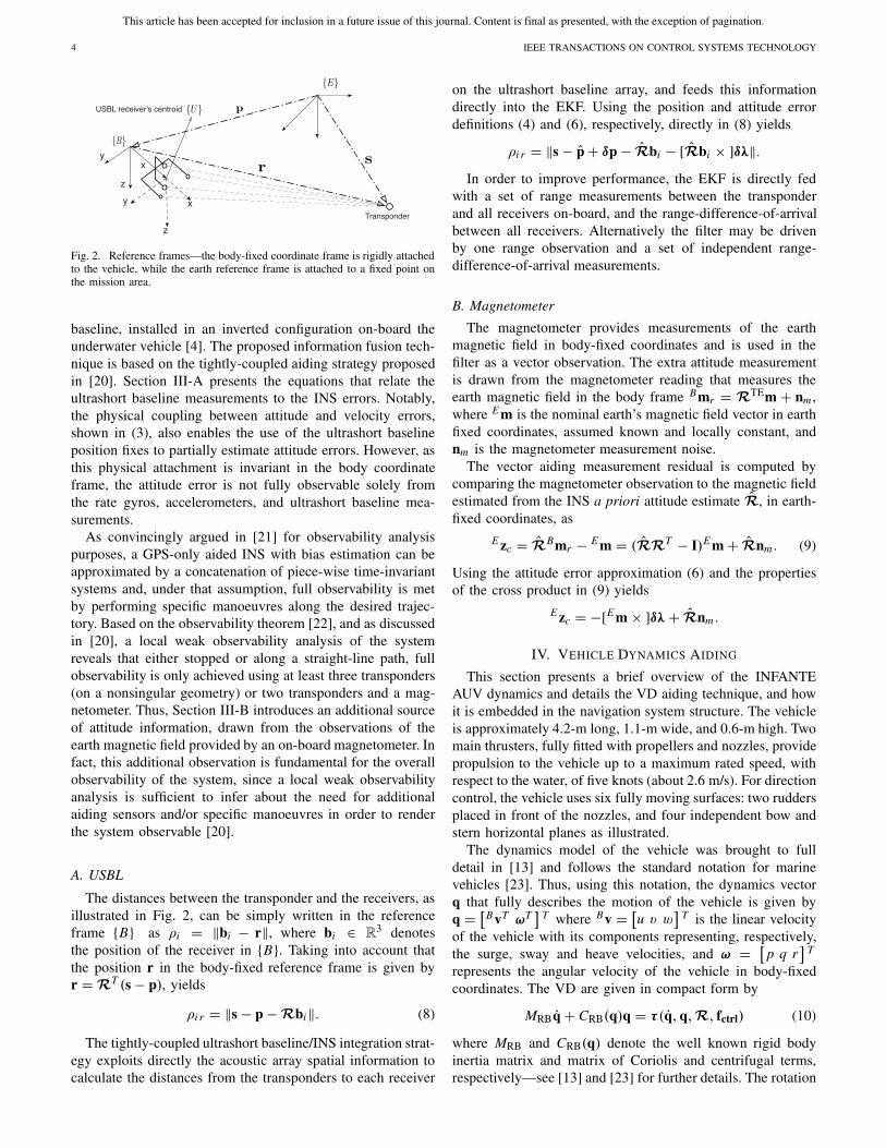
Fig. 2. Reference frames—the body-fixed coordinate frame is rigidly attachedto the vehicle, while the earth reference frame is attached to a fixed point onthe mission area.

baseline, installed in an inverted configuration on-board theunderwater vehicle [4]. The proposed information fusion tech-nique is based on the tightly-coupled aiding strategy proposedin [20]. Section III-A presents the equations that relate theultrashort baseline measurements to the INS errors. Notably,the physical coupling between attitude and velocity errors,shown in (3), also enables the use of the ultrashort baselineposition fixes to partially estimate attitude errors. However, asthis physical attachment is invariant in the body coordinateframe, the attitude error is not fully observable solely fromthe rate gyros, accelerometers, and ultrashort baseline mea-surements.

As convincingly argued in [21] for observability analysispurposes, a GPS-only aided INS with bias estimation can beapproximated by a concatenation of piece-wise time-invariantsystems and, under that assumption, full observability is metby performing specific manoeuvres along the desired trajec-tory. Based on the observability theorem [22], and as discussedin [20], a local weak observability analysis of the systemreveals that either stopped or along a straight-line path, fullobservability is only achieved using at least three transponders(on a nonsingular geometry) or two transponders and a mag-netometer. Thus, Section III-B introduces an additional sourceof attitude information, drawn from the observations of theearth magnetic field provided by an on-board magnetometer. Infact, this additional observation is fundamental for the overallobservability of the system, since a local weak observabilityanalysis is sufficient to infer about the need for additionalaiding sensors and/or specific manoeuvres in order to renderthe system observable [20].

A. USBL

The distances between the transponder and the receivers, asillustrated in Fig. 2, can be simply written in the referenceframe {B} as ρi = ‖bi − r‖, where bi ∈ R

3 denotesthe position of the receiver in {B}. Taking into account thatthe position r in the body-fixed reference frame is given byr = RT (s − p), yields

ρi r = ‖s − p − Rbi‖. (8)

The tightly-coupled ultrashort baseline/INS integration strat-egy exploits directly the acoustic array spatial information tocalculate the distances from the transponders to each receiver

on the ultrashort baseline array, and feeds this informationdirectly into the EKF. Using the position and attitude errordefinitions (4) and (6), respectively, directly in (8) yields

ρi r = ‖s − p + δp − Rbi − [Rbi × ]δλ‖.In order to improve performance, the EKF is directly fed

with a set of range measurements between the transponderand all receivers on-board, and the range-difference-of-arrivalbetween all receivers. Alternatively the filter may be drivenby one range observation and a set of independent range-difference-of-arrival measurements.

B. Magnetometer

The magnetometer provides measurements of the earthmagnetic field in body-fixed coordinates and is used in thefilter as a vector observation. The extra attitude measurementis drawn from the magnetometer reading that measures theearth magnetic field in the body frame Bmr = RTEm + nm ,where E m is the nominal earth’s magnetic field vector in earthfixed coordinates, assumed known and locally constant, andnm is the magnetometer measurement noise.

The vector aiding measurement residual is computed bycomparing the magnetometer observation to the magnetic fieldestimated from the INS a priori attitude estimate R, in earth-fixed coordinates, as

E zc = RBmr − E m = (RRT − I)E m + Rnm . (9)

Using the attitude error approximation (6) and the propertiesof the cross product in (9) yields

E zc = −[E m × ]δλ + Rnm .

IV. VEHICLE DYNAMICS AIDING

This section presents a brief overview of the INFANTEAUV dynamics and details the VD aiding technique, and howit is embedded in the navigation system structure. The vehicleis approximately 4.2-m long, 1.1-m wide, and 0.6-m high. Twomain thrusters, fully fitted with propellers and nozzles, providepropulsion to the vehicle up to a maximum rated speed, withrespect to the water, of five knots (about 2.6 m/s). For directioncontrol, the vehicle uses six fully moving surfaces: two ruddersplaced in front of the nozzles, and four independent bow andstern horizontal planes as illustrated.

The dynamics model of the vehicle was brought to fulldetail in [13] and follows the standard notation for marinevehicles [23]. Thus, using this notation, the dynamics vectorq that fully describes the motion of the vehicle is given byq = [

BvT ωT]

T where Bv = [u v w

]T is the linear velocity

of the vehicle with its components representing, respectively,the surge, sway and heave velocities, and ω = [

p q r]

T

represents the angular velocity of the vehicle in body-fixedcoordinates. The VD are given in compact form by

MRBq + CRB(q)q = τ (q, q,R, fctrl) (10)

where MRB and CRB(q) denote the well known rigid bodyinertia matrix and matrix of Coriolis and centrifugal terms,respectively—see [13] and [23] for further details. The rotation



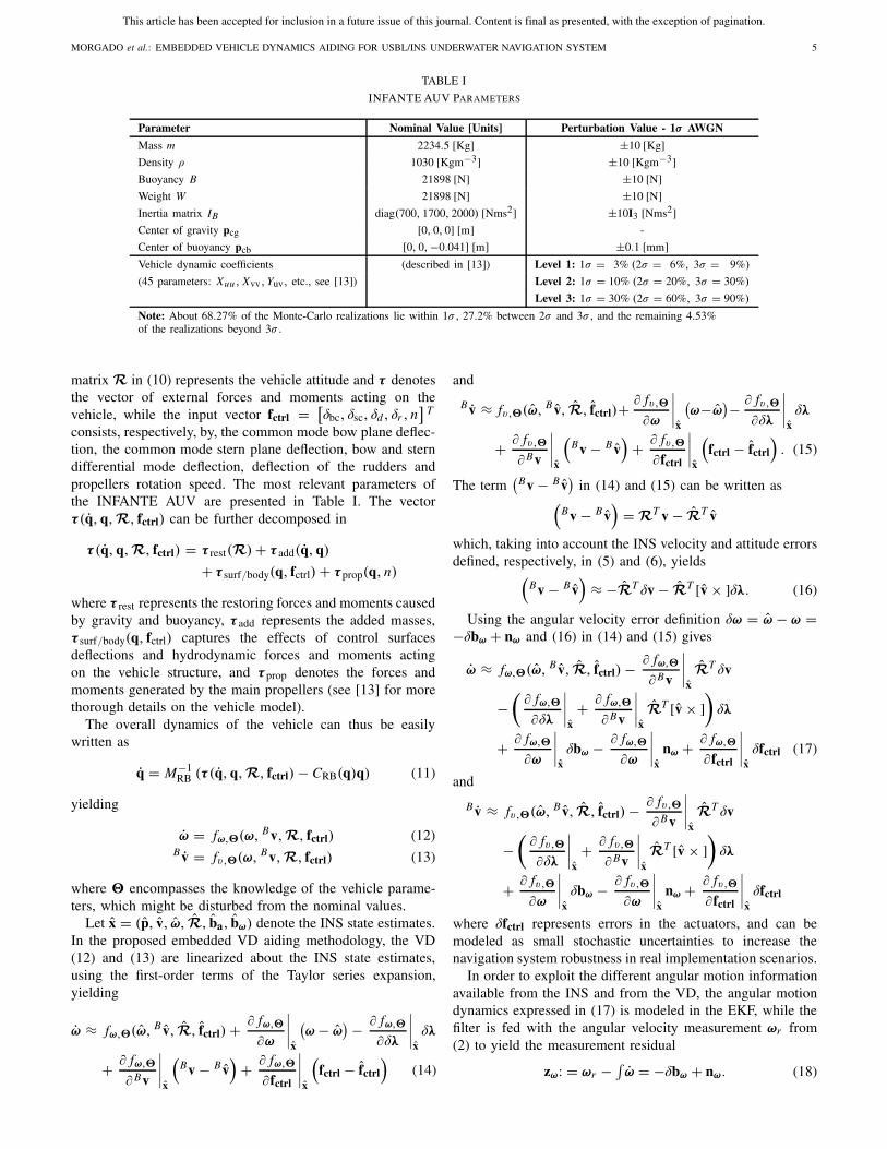
TABLE I

INFANTE AUV PARAMETERS

Parameter Nominal Value [Units] Perturbation Value - 1σ AWGN

Mass m 2234.5 [Kg] ±10 [Kg]

Density ρ 1030 [Kgm−3] ±10 [Kgm−3]

Buoyancy B 21898 [N] ±10 [N]

Weight W 21898 [N] ±10 [N]

Inertia matrix IB diag(700, 1700, 2000) [Nms2] ±10I3 [Nms2]

Center of gravity pcg [0, 0, 0] [m] -

Center of buoyancy pcb [0, 0,−0.041] [m] ±0.1 [mm]

Vehicle dynamic coefficients (described in [13]) Level 1: 1σ = 3% (2σ = 6%, 3σ = 9%)

(45 parameters: Xuu , Xvv, Yuv, etc., see [13]) Level 2: 1σ = 10% (2σ = 20%, 3σ = 30%)

Level 3: 1σ = 30% (2σ = 60%, 3σ = 90%)

Note: About 68.27% of the Monte-Carlo realizations lie within 1σ , 27.2% between 2σ and 3σ , and the remaining 4.53%of the realizations beyond 3σ .

matrix R in (10) represents the vehicle attitude and τ denotesthe vector of external forces and moments acting on thevehicle, while the input vector fctrl = [

δbc, δsc, δd , δr , n]

T

consists, respectively, by, the common mode bow plane deflec-tion, the common mode stern plane deflection, bow and sterndifferential mode deflection, deflection of the rudders andpropellers rotation speed. The most relevant parameters ofthe INFANTE AUV are presented in Table I. The vectorτ (q, q,R, fctrl) can be further decomposed in

τ (q, q,R, fctrl) = τ rest(R) + τ add(q, q)

+ τ surf/body(q, fctrl) + τ prop(q, n)

where τ rest represents the restoring forces and moments causedby gravity and buoyancy, τ add represents the added masses,τ surf/body(q, fctrl) captures the effects of control surfacesdeflections and hydrodynamic forces and moments actingon the vehicle structure, and τ prop denotes the forces andmoments generated by the main propellers (see [13] for morethorough details on the vehicle model).

The overall dynamics of the vehicle can thus be easilywritten as

q = M−1RB (τ (q, q,R, fctrl) − CRB(q)q) (11)

yielding

ω = fω,�(ω, Bv,R, fctrl) (12)B v = fv,�(ω, Bv,R, fctrl) (13)

where � encompasses the knowledge of the vehicle parame-ters, which might be disturbed from the nominal values.

Let x = (p, v, ω, R, ba, bω) denote the INS state estimates.In the proposed embedded VD aiding methodology, the VD(12) and (13) are linearized about the INS state estimates,using the first-order terms of the Taylor series expansion,yielding

ω ≈ fω,�(ω, B v, R, fctrl) + ∂ fω,�

∂ω

∣∣∣∣x

(ω − ω

) − ∂ fω,�

∂δλ

∣∣∣∣xδλ

+ ∂ fω,�

∂ Bv

∣∣∣∣x

(Bv − B v

)+ ∂ fω,�

∂fctrl

∣∣∣∣x

(fctrl − fctrl

)(14)

and

B v ≈ fv,�(ω, B v, R, fctrl)+ ∂ fv,�

∂ω

∣∣∣∣x

(ω−ω

)− ∂ fv,�

∂δλ

∣∣∣∣xδλ

+ ∂ fv,�

∂ Bv

∣∣∣∣x

(Bv − B v

)+ ∂ fv,�

∂fctrl

∣∣∣∣x

(fctrl − fctrl

). (15)

The term(

Bv − B v)

in (14) and (15) can be written as(

Bv − B v)

= RT v − RT v

which, taking into account the INS velocity and attitude errorsdefined, respectively, in (5) and (6), yields

(Bv − B v

)≈ −RT δv − RT [v × ]δλ. (16)

Using the angular velocity error definition δω = ω − ω =−δbω + nω and (16) in (14) and (15) gives

ω ≈ fω,�(ω, B v, R, fctrl) − ∂ fω,�

∂ Bv

∣∣∣∣xRT δv

−(

∂ fω,�

∂δλ

∣∣∣∣x+ ∂ fω,�

∂ Bv

∣∣∣∣xRT [v × ]

)δλ

+ ∂ fω,�

∂ω

∣∣∣∣xδbω − ∂ fω,�

∂ω

∣∣∣∣x

nω + ∂ fω,�

∂fctrl

∣∣∣∣xδfctrl (17)

and

B v ≈ fv,�(ω, B v, R, fctrl) − ∂ fv,�

∂ Bv

∣∣∣∣xRT δv

−(

∂ fv,�

∂δλ

∣∣∣∣x+ ∂ fv,�

∂ Bv

∣∣∣∣xRT [v × ]

)δλ

+ ∂ fv,�

∂ω

∣∣∣∣xδbω − ∂ fv,�

∂ω

∣∣∣∣x

nω + ∂ fv,�

∂fctrl

∣∣∣∣xδfctrl

where δfctrl represents errors in the actuators, and can bemodeled as small stochastic uncertainties to increase thenavigation system robustness in real implementation scenarios.

In order to exploit the different angular motion informationavailable from the INS and from the VD, the angular motiondynamics expressed in (17) is modeled in the EKF, while thefilter is fed with the angular velocity measurement ωr from(2) to yield the measurement residual

zω: = ωr − ∫ω = −δbω + nω. (18)



TABLE II

SENSORS AWGN CHARACTERISTICS

Sensor Bias 1σ STD

Accelerometer (Crossbow CXL02TG3) 12 mg 0.6 mg

Rate gyro (Silicon Sensing CRS03) 5 deg/s 0.05 deg/s

Magnetometer (Crossbow CXM113) - 60 μGauss

USBL range - 0.3 m

USBL RDOA - 6 mm

USBL elevation and azimuth - 0.4 deg

TABLE III

INITIAL ESTIMATES ERROR CHARACTERISTICS

Initial estimate 1σ STD

Position 5 m

Velocity 0.5 m/s

Attitude 1 deg

where∫ω is numerically integrated in the EKF, from (12)

evaluated at the estimated state (ω, B v, R, fctrl).The dynamics of Bv expressed in (13) are used to feed the

filter with the measurement residual

zv: = fv,�(ω, B v, R, fctrl) − B ˙v (19)

where B ˙v is drawn from the accelerometer measurements (1)and allows for (19) to be rewritten [12] as

zv =(

[ω × ] + ∂ fv,�

∂ Bv

∣∣∣∣x

)RT δv− ∂ fv,�

∂fctrl

∣∣∣∣xδfctrl + δba − na

+(

[ω × ][B v × ] − [B g × ]

+∂ fv,�

∂δλ

∣∣∣∣xR + ∂ fv,�

∂ Bv

∣∣∣∣x[B v × ]

)RT δλ

+(

[B v × ]− ∂ fv,�

∂ω

∣∣∣∣x

)δbω+

(∂ fv,�

∂ω

∣∣∣∣x−[B v × ]

)nω.

(20)

Remark 1 (Implementation Remark): Special care must betaken in the implementation of the VD aiding techniqueoutlined herein, since the observation noise present in theVD measurement residuals (18) and (20) is correlated to thestate noise in (3). Thus, this information about the correlationbetween the state and observation noise must be included inthe filter implementation using modified algebraic equationsfor the update cycle of the EKF, as described in [24], with noadditional states necessary.

V. NUMERICAL RESULTS AND PERFORMANCE

EVALUATION

The performance of the proposed VD aiding techniquewas assessed with the model of the INFANTE AUV. Thefiltering setup is exposed to extensive Monte Carlo simula-tions, with different initial conditions and multiple sensorsnoise sequences (disturbances characteristics are described inTable II and initial estimates deviations in Table III). Thissection presents the simulation setup, including the underwater

USBL outage[90, 110] s

USBL outage[160, 180] s

Underwater current

[125, 185] sIntensity = 0.1 m/s

Direction = 110 degHorizontal plane

Fig. 3. Vehicle trajectory—the vehicle starts moving forward at a depth ofabout 10 m, and then needs to go slightly up to pitch down and dive at aconstant rate while performing a snake-like trajectory.

current disturbance description, and the results analysis anddiscussion.

A. Simulation Setup

The vehicle follows the trajectory depicted in Fig. 3. Attime t = 125 s, an underwater current with an intensityof 0.1 m/s, is introduced flowing in the horizontal planefrom a direction of 110 deg for 60 s. The simulation time is200 s, which was found sufficient for the filters to achievea steady-state behavior, that is representative of long-termoperating conditions. Two 20 s periods of ultrashort baselinesensor outages are included at the intervals t = [90, 110] sand t = [160, 180] s. The vehicle aiding measurements andcomputations are processed at the same rate of the moderatespeed INS computations rate, which is set to 50 Hz. Thehigh-speed INS computations are executed at a higher rateof 100 Hz. The ultrashort baseline receiving array providesmeasurements once per second and is composed of fourreceivers that are installed on the vehicle, 30 cm awayfrom the strap-down inertial measurement unit (IMU) setup(along the x-axis of the body-fixed coordinate frame {B}).Thus, the positions of the receivers with respect to {B} aregiven by b1 = [0.2 − 0.15 0]T m, b2 = [0.2 0.15 0]T m,b3 = [0.4 0 0.15]T m, and b4 = [0.4 0 − 0.15]T m. Thetransponder is located in local inertial coordinates at E pt =[0 200 0]T m.

The sensors noise characteristics are summarized in Table II.The inertial sensors and magnetometers parameters are basedon realistic commercially available sensor packages, and theinverted ultrashort baseline positioning system was fully devel-oped in-house. The triaxial inertial sensors data is gener-ated in simulation by adding the bias and additive whiteGaussian noise (AWGN) described in Table II, to the datagenerated by the nominal VD model, and according to(1) and (2). A triaxial magnetometer is also used in the pro-posed solution, as described in Section III-B, which is assumedcalibrated for bias, scale factors, and nonorthogonality of theinput axis. The simulated magnetometer data is generatedby adding the described additive white Gaussian noise to



the nominal magnetic field vector represented in the bodycoordinate frame (obtained as described in Section III-B andusing the nominal vehicle model). Even with the addition ofthe external magnetic field vector observation, using only onetransponder is not sufficient to obtain full state observabilityduring straight line manoeuvres, as carefully discussed in[20]. Hence, the need for turning/diving manoeuvres built intothe nominal trajectory, which is of paramount importance forobservability enhancement purposes, and especially during theinitial alignment phase.

Adding the corresponding additive white Gaussian noise tothe nominal ranges and range-difference-of-arrival generatesthe ultrashort baseline data. All sensor data is generated insimulation using the vehicle model with the nominal parameterset (represented by � in Fig. 1), corrupted by noise and bias.The embedded models (nonnominal or perturbed) generate theVD aiding information inside the EKF using the perturbed(nonnominal) parameter set (represented by � in Fig. 1 andin Section IV). Sensor modeling errors can be compensated inthe filters using inflated noise [25], among other techniques,that are beyond the scope of this brief and should be assessedin experimental applications of the navigation system.

B. Underwater Current Disturbance

The underwater current that disturbs the trajectory of thevehicle is assumed irrotational, such that each infinitesimalfluid element has zero angular velocity or spin (even if thiscurrent moves along a circle, i.e., changes direction over time)[10]. Under the irrotational current assumption, the vehiclemodel described in (11) is also valid considering water-relativevelocity components [10, Property 2], that is

qr = M−1RB (τ (qr , qr ,R, fctrl) − CRB(qr )qr ) (21)

where qr represents the linear and angular velocities of thevehicle relative to an irrotational underwater current withvelocity vc ∈ R

3, such that

qr = q + [vcT R 01×3]T .

Note that the current velocity components related to theangular velocities of q are null, due to the irrotational currentassumption. The expression in (21) is also valid for the zero-current case, for which vc = 03×1 and qr = q. Thus, theabove-mentioned underwater current disturbance in simulationis added by setting a nonzero underwater current velocity vc onthe right side of (21), and according to Fig. 1 before generatingthe simulated inertial sensors data. As illustrated in Fig. 1, theperturbed VD models that are embedded in the EKF, do notconsider the underwater current disturbance.

C. Results Discussion

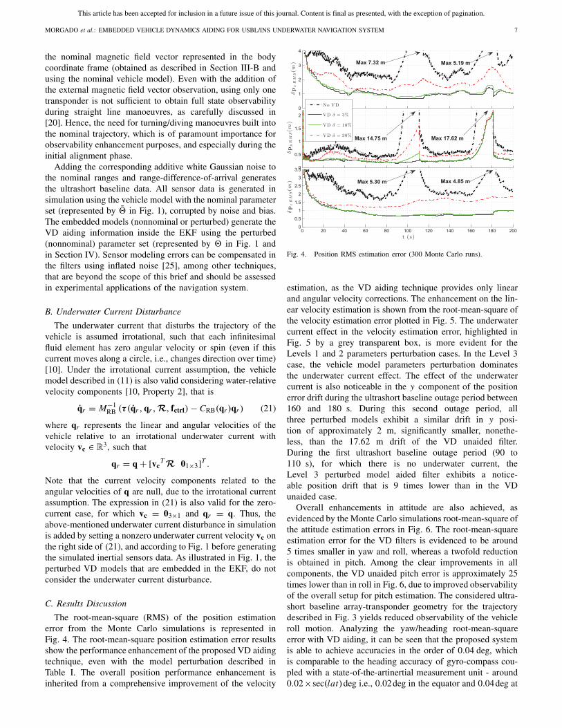
The root-mean-square (RMS) of the position estimationerror from the Monte Carlo simulations is represented inFig. 4. The root-mean-square position estimation error resultsshow the performance enhancement of the proposed VD aidingtechnique, even with the model perturbation described inTable I. The overall position performance enhancement isinherited from a comprehensive improvement of the velocity

Fig. 4. Position RMS estimation error (300 Monte Carlo runs).

estimation, as the VD aiding technique provides only linearand angular velocity corrections. The enhancement on the lin-ear velocity estimation is shown from the root-mean-square ofthe velocity estimation error plotted in Fig. 5. The underwatercurrent effect in the velocity estimation error, highlighted inFig. 5 by a grey transparent box, is more evident for theLevels 1 and 2 parameters perturbation cases. In the Level 3case, the vehicle model parameters perturbation dominatesthe underwater current effect. The effect of the underwatercurrent is also noticeable in the y component of the positionerror drift during the ultrashort baseline outage period between160 and 180 s. During this second outage period, allthree perturbed models exhibit a similar drift in y posi-tion of approximately 2 m, significantly smaller, nonethe-less, than the 17.62 m drift of the VD unaided filter.During the first ultrashort baseline outage period (90 to110 s), for which there is no underwater current, theLevel 3 perturbed model aided filter exhibits a notice-able position drift that is 9 times lower than in the VDunaided case.

Overall enhancements in attitude are also achieved, asevidenced by the Monte Carlo simulations root-mean-square ofthe attitude estimation errors in Fig. 6. The root-mean-squareestimation error for the VD filters is evidenced to be around5 times smaller in yaw and roll, whereas a twofold reductionis obtained in pitch. Among the clear improvements in allcomponents, the VD unaided pitch error is approximately 25times lower than in roll in Fig. 6, due to improved observabilityof the overall setup for pitch estimation. The considered ultra-short baseline array-transponder geometry for the trajectorydescribed in Fig. 3 yields reduced observability of the vehicleroll motion. Analyzing the yaw/heading root-mean-squareerror with VD aiding, it can be seen that the proposed systemis able to achieve accuracies in the order of 0.04 deg, whichis comparable to the heading accuracy of gyro-compass cou-pled with a state-of-the-artinertial measurement unit - around0.02×sec(lat)deg i.e., 0.02 deg in the equator and 0.04deg at



Fig. 5. Velocity RMS estimation error (300 Monte Carlo runs).

Fig. 6. Attitude RMS estimation error (300 Monte Carlo runs).

Fig. 7. Vehicle model numerically integrated linear velocity RMS error(300 Monte Carlo runs). The VD model aiding technique presented in thisbrief does not use this quantity, using directly linear acceleration observationsdrawn from the inertial sensor measurements and the linear accelerationprovided by the VD model.

a latitude of ±60 deg. Despite the lack of a gyro-compassin the solution proposed herein, that level of performanceis achievable due to the combination of a low-cost inertialmeasurement unit and three additional sources of information:

Fig. 8. Vehicle model provided linear acceleration RMS error (300 MonteCarlo runs).

Fig. 9. Vehicle model provided angular velocity RMS error (300 MonteCarlo runs).

velocity readings from the VD model, earth magnetic fieldvector from the triaxial magnetometers, and ultrashort baselineposition fixes. The combination of these sensors in a fullyintegrated package ultimately yields improved observabilityand attitude accuracy comparable to state-of-the-art IMU andgyro-compasses.

The linear velocity output root-mean-square error, from theconsidered VD perturbed models, is represented in Fig. 7,illustrating the difference between the nominal model out-put (with the underwater current disturbance included) andthe outputs from the perturbed vehicle models. Interestinglyenough, linear velocity corrections are fed directly to the filteras observations of linear acceleration drawn from the inertialsensor measurements, as given by (19), and no integrationmethods for the VD velocity are adopted as in classicalexternal VD aiding techniques. Consequently, the integrationof velocity aiding requires no more computational resourcesthan those of a state update. Nonetheless, the numericalintegration of the angular velocity dynamics is easily exe-cuted with an explicit fourth-order Runge–Kutta integrationalgorithm, making it suitable for implementation in low-powerconsumption hardware. The root-mean-square of the linearacceleration observations that are fed to the filters is illustratedin Fig. 8, which includes a zoom to better visualize thedifference between the output root-mean-square errors of thethree perturbation levels. The model-aided filter also uses thenumerically integrated angular velocity from the perturbed VDmodels, using (18) and whose observations root-mean-squareerrors are illustrated in Fig. 9 for each of the VD parametersperturbation level. The information provided in Figs. 8 and 9allows for assessing the discrepancy between the informationprovided by VD perturbed models and from the ground-truthinformation (of the nominal model) available from the on-



board sensors. Note that the filter did not diverge in any of theMonte Carlo runs, evidencing the robustness of the proposedtechnique under vehicle modeling errors. The performanceenhancement is evident not only from the steady-state responseof the filters, but also during the initial convergence phase fromerroneous initial conditions.

VI. CONCLUSION

An embedded VD inclusion technique was successfullyadopted in this brief to enhance position, velocity, and attitudeestimates of low-cost INS. The performance of the proposedVD aiding technique was assessed with the dynamics modelof the INFANTE AUV, designed, and developed at IST/ISRin Lisbon, resorting to extensive Monte Carlo simulations inwhich the filtering setup is exposed to different initial condi-tions and all the sensors to different noise sequences. Fromthe thorough results analysis of 300 Monte Carlo runs, theproposed VD aiding technique was shown to yield significantlyimproved performance compared to the VD unaided solution,in the presence of realistic sensor noise. The navigation systemalso exhibited robustness to disturbances on the vehicle model,which is a desirable feature on the practical design of naviga-tion systems. The overall improvements in position estimationcan be summarized as follows: for parameter perturbation withstandard deviations of 3% and 10%, position estimation erroris 2.5 times lower than in the VD unaided case, whereasfor perturbations with a standard deviation of 30% the erroris around 1.5 times lower than in the VD unaided case.During ultrashort baseline outages and without underwatercurrent, the filters only revealed noticeable position drift forthe perturbation Level 3, nonetheless 9 times smaller thanin the VD unaided case. With the presence of underwatercurrents, position estimate drifts are not evident until anultrashort baseline drop-out occurs, during which the positionerror drift is in line with the integration of the underwatercurrent but still nine times less than in the VD unaided case.Enhancements in attitude estimation were likewise achievedwith twofold error reduction for pitch angle estimation andfivefold for yaw and roll angles. None of the Monte Carlo runsrevealed divergence of the filter, emphasizing the robustnessof the proposed technique under vehicle model parametererrors (three disturbance levels with up to 1σ perturbationvalues of 30% in the vehicle model parameter errors). Theexplicit estimation of the underwater current disturbance wasnot addressed in this brief, in which the main contributionis centered on the validation of the embedded VD modelaiding technique for underwater vehicles. Note that, on onehand, modeling the underwater current in the filter couldimprove filter robustness, but, on the other, it could intro-duce filter divergence due to modeling errors, and potentialnonobservability of the augmented state space. Future workwill focus on this subject and on the implementation and real-world validation of the proposed technique with an underwatervehicle.

REFERENCES

[1] J. Kinsey, R. Eustice, and L. Whitcomb, “A survey of underwater vehiclenavigation: Recent advances and new challenges,” in Proc. 7th IFACConf. Manoeuvr. Control Marine Craft, 2006, pp. 1–12.

[2] R. Brown and P. Hwang, Introduction to Random Signals and AppliedKalman Filtering, 3rd ed. New York, USA: Wiley, 1997.

[3] P. H. Milne, Underwater Acoustic Positioning Systems. Houston, TX,USA: Gulf, 1983.

[4] K. Vickery, “Acoustic positioning systems. new concepts—The future,”in Proc. Workshop Auto. Underwater Veh., Aug. 1998, pp. 103–110.

[5] X. Lurton and N. Millard, “The feasibility of a very-long baselineacoustic positioning system for AUVs,” in Proc. IEEE Oceans Eng.Today’s Technol. Tomorrow’s Preservat. Conf., vol. 3. Sep. 1994,pp. 403–408.

[6] S. Smith and D. Kronen, “Experimental results of an inexpensive shortbaseline acoustic positioning system for AUV navigation,” in Proc.MTS/IEEE Oceans Conf., vol. 1. Oct. 1997, pp. 714–720.

[7] M. Koifman and I. Y. Bar-Itzhack, “Inertial navigation system aided byaircraft dynamics,” IEEE Trans. Control Syst. Technol., vol. 7, no. 4,pp. 487–493, Jul. 1999.

[8] S. J. Julier and H. F. Durrant-Whyte, “On The role of process modelsin autonomous land vehicle navigation systems,” IEEE Trans. Robot.Autom., vol. 19, no. 1, pp. 1–14, Feb. 2003.

[9] M. Bryson and S. Sukkarieh, “Vehicle model aided inertial navigation fora UAV using low-cost sensors,” in Proc. Austral. Conf. Robot. Autom.,Dec. 2004, pp. 1–9.

[10] O. Hegrenaes and O. Hallingstad, “Model-aided INS withsea current estimation for robust underwater navigation,”IEEE J. Ocean. Eng., vol. 36, no. 2, pp. 316–337,Apr. 2011.

[11] G. Dissanayake and S. Sukkarieh, “The aiding of a low-cost strap-down inertial measurement unit using vehicle model constraints forland vehicle application,” IEEE Trans. Robot. Autom., vol. 17, no. 5,pp. 731–747, Oct. 2001. X

[12] J. F. Vasconcelos, C. Silvestre, P. Oliveira, and B. Guerreiro, “Embed-ded UAV model and LASER aiding techniques for inertial navigationsystems,” Control Eng. Pract., vol. 18, no. 3, pp. 262–278, Mar. 2010.

[13] C. Silvestre and A. Pascoal, “Control of the INFANTE AUV using gainscheduled static output feedback,” Control Eng. Pract., vol. 12, no. 12,pp. 1501–1509, Dec. 2004.

[14] C. Silvestre, R. Cunha, N. Paulino, and A. Pascoal, “A bottom-following preview controller for autonomous underwater vehicles,”IEEE Trans. Control Syst. Technol., vol. 17, no. 2, pp. 257–266,Mar. 2009.

[15] M. Morgado, P. Oliveira, C. Silvestre, and J. F. Vasconcelos, “Vehi-cle dynamics aiding technique for USBL/INS underwater navigationsystem,” in Proc. IFAC Conf. Control Appl. Marine Syst., Sep. 2007,pp. 1–6.

[16] P. Savage, “Strapdown inertial navigation integration algorithm designpart 1: Attitude algorithms,” J. Guid. Control Dyn., vol. 21, no. 1,pp. 19–28, Jan.–Feb. 1998.

[17] P. G. Savage, “Strapdown inertial navigation integration algorithm designpart 2: Velocity and position algorithms,” J. Guid. Control Dyn, vol. 21,no. 2, pp. 208–221, Mar.–Apr. 1998.

[18] J. F. Vasconcelos, C. Silvestre, and P. Oliveira, “INS/GPS aided by fre-quency contents of vector observations with application to autonomoussurface crafts,” IEEE. J. Ocean. Eng., vol. 36, no. 2, pp. 347–363,Apr. 2011.

[19] K. R. Britting, Inertial Navigation Systems Analysis. New York, USA:Wiley, 1971.

[20] M. Morgado, P. Oliveira, C. Silvestre, and J. F. Vasconcelos, “USBL/INStightly-coupled integration technique for underwater vehicles,” in Proc.9th Int. Conf. Inf. Fusion, Jul. 2006, pp. 1–8.

[21] D. Goshen-Meskin and I. Y. Bar-Itzhack, “Observability analysis ofpiece-wise constant systems—Part II: Application to inertial navigationin-flight alignment,” IEEE Trans. Aerosp. Electron. Syst., vol. 28, no. 4,pp. 1068–1075, Oct. 1992.

[22] W. Rugh, Linear System Theory, 2nd ed. Englewood Cliffs, NJ, USA:Prentice-Hall, 1996.

[23] T. Fossen, Guidance and Control of Ocean Vehicles. New York, USA:Wiley, 1994.

[24] A. Gelb, Applied Optimal Estimation. Cambridge, MA, USA: MITPress, 1974.

[25] A. H. Jazwinski, Stochastic Processes and Filtering Theory, vol. 64.New York, USA: Academic, 1970.

embedded vehicle dynamics aiding for usbl/ins underwater...

Documents