embedded linux primer: a practical real-world approach
TRANSCRIPT


Embedded Linux Primer: A Practical, Real-World Approach
By Christopher Hallinan
...............................................
Publisher: Prentice Hall
Pub Date: September 18, 2006
Print ISBN-10: 0-13-167984-8
Print ISBN-13: 978-0-13-167984-9
Pages: 576
Table of Contents | Index
Comprehensive Real-World Guidance for Every Embedded Developer and Engineer
This book brings together indispensable knowledge for building efficient, high-value, Linux-basedembedded products: information that has never been assembled in one place before. Drawing onyears of experience as an embedded Linux consultant and field application engineer, ChristopherHallinan offers solutions for the specific technical issues you're most likely to face, demonstrateshow to build an effective embedded Linux environment, and shows how to use it as productively aspossible.
Hallinan begins by touring a typical Linux-based embedded system, introducing key concepts andcomponents, and calling attention to differences between Linux and traditional embeddedenvironments. Writing from the embedded developer's viewpoint, he thoroughly addresses issuesranging from kernel building and initialization to bootloaders, device drivers to file systems.
Hallinan thoroughly covers the increasingly popular BusyBox utilities; presents a step-by-stepwalkthrough of porting Linux to custom boards; and introduces real-time configuration viaCONFIG_RT--one of today's most exciting developments in embedded Linux. You'll find especiallydetailed coverage of using development tools to analyze and debug embedded systems--includingthe art of kernel debugging.
Compare leading embedded Linux processors
Understand the details of the Linux kernel initialization process
Learn about the special role of bootloaders in embedded Linux systems, with specific emphasison U-Boot
Use embedded Linux file systems, including JFFS2--with detailed guidelines for building Flash-resident file system images
Understand the Memory Technology Devices subsystem for flash (and other) memory devices
Master gdb, KGDB, and hardware JTAG debugging
Learn many tips and techniques for debugging within the Linux kernel

Maximize your productivity in cross-development environments
Prepare your entire development environment, including TFTP, DHCP, and NFS target servers
Configure, build, and initialize BusyBox to support your unique requirements
About the Author
Christopher Hallinan, field applications engineer at MontaVista software, has worked for more than20 years in assignments ranging from engineering and engineering management to marketing andbusiness development. He spent four years as an independent development consultant in theembedded Linux marketplace. His work has appeared in magazines, including TelecommunicationsMagazine, Fiber Optics Magazine, and Aviation Digest.

Embedded Linux Primer: A Practical, Real-World Approach
By Christopher Hallinan
...............................................
Publisher: Prentice Hall
Pub Date: September 18, 2006
Print ISBN-10: 0-13-167984-8
Print ISBN-13: 978-0-13-167984-9
Pages: 576
Table of Contents | Index
Copyright
Prentice Hall Open Source Software Development Series
Foreword
Preface
Acknowledgments
About the Author
Chapter 1. Introduction
Section 1.1. Why Linux?
Section 1.2. Embedded Linux Today
Section 1.3. Open Source and the GPL
Section 1.4. Standards and Relevant Bodies
Section 1.5. Chapter Summary
Chapter 2. Your First Embedded Experience
Section 2.1. Embedded or Not?
Section 2.2. Anatomy of an Embedded System
Section 2.3. Storage Considerations
Section 2.4. Embedded Linux Distributions
Section 2.5. Chapter Summary
Chapter 3. Processor Basics
Section 3.1. Stand-alone Processors
Section 3.2. Integrated Processors: Systems on Chip
Section 3.3. Hardware Platforms
Section 3.4. Chapter Summary
Chapter 4. The Linux KernelA Different Perspective
Section 4.1. Background
Section 4.2. Linux Kernel Construction
Section 4.3. Kernel Build System
Section 4.4. Obtaining a Linux Kernel
Section 4.5. Chapter Summary
Chapter 5. Kernel Initialization
Section 5.1. Composite Kernel Image: Piggy and Friends
Section 5.2. Initialization Flow of Control

Section 5.3. Kernel Command Line Processing
Section 5.4. Subsystem Initialization
Section 5.5. The init Thread
Section 5.6. Chapter Summary
Chapter 6. System Initialization
Section 6.1. Root File System
Section 6.2. Kernel's Last Boot Steps
Section 6.3. The Init Process
Section 6.4. Initial RAM Disk
Section 6.5. Using initramfs
Section 6.6. Shutdown
Section 6.7. Chapter Summary
Chapter 7. Bootloaders
Section 7.1. Role of a Bootloader
Section 7.2. Bootloader Challenges
Section 7.3. A Universal Bootloader: Das U-Boot
Section 7.4. Porting U-Boot
Section 7.5. Other Bootloaders
Section 7.6. Chapter Summary
Chapter 8. Device Driver Basics
Section 8.1. Device Driver Concepts
Section 8.2. Module Utilities
Section 8.3. Driver Methods
Section 8.4. Bringing It All Together
Section 8.5. Device Drivers and the GPL
Section 8.6. Chapter Summary
Chapter 9. File Systems
Section 9.1. Linux File System Concepts
Section 9.2. ext2
Section 9.3. ext3
Section 9.4. ReiserFS
Section 9.5. JFFS2
Section 9.6. cramfs
Section 9.7. Network File System
Section 9.8. Pseudo File Systems
Section 9.9. Other File Systems
Section 9.10. Building a Simple File System
Section 9.11. Chapter Summary
Chapter 10. MTD Subsystem
Section 10.1. Enabling MTD Services
Section 10.2. MTD Basics
Section 10.3. MTD Partitions
Section 10.4. MTD Utilities
Section 10.5. Chapter Summary
Chapter 11. BusyBox
Section 11.1. Introduction to BusyBox

Section 11.2. BusyBox Configuration
Section 11.3. BusyBox Operation
Section 11.4. Chapter Summary
Chapter 12. Embedded Development Environment
Section 12.1. Cross-Development Environment
Section 12.2. Host System Requirements
Section 12.3. Hosting Target Boards
Section 12.4. Chapter Summary
Chapter 13. Development Tools
Section 13.1. GNU Debugger (GDB)
Section 13.2. Data Display Debugger
Section 13.3. cbrowser/cscope
Section 13.4. Tracing and Profiling Tools
Section 13.5. Binary Utilities
Section 13.6. Miscellaneous Binary Utilities
Section 13.7. Chapter Summary
Chapter 14. Kernel Debugging Techniques
Section 14.1. Challenges to Kernel Debugging
Section 14.2. Using KGDB for Kernel Debugging
Section 14.3. Debugging the Linux Kernel
Section 14.4. Hardware-Assisted Debugging
Section 14.5. When It Doesn't Boot
Section 14.6. Chapter Summary
Chapter 15. Debugging Embedded Linux Applications
Section 15.1. Target Debugging
Section 15.2. Remote (Cross) Debugging
Section 15.3. Debugging with Shared Libraries
Section 15.4. Debugging Multiple Tasks
Section 15.5. Additional Remote Debug Options
Section 15.6. Chapter Summary
Chapter 16. Porting Linux
Section 16.1. Linux Source Organization
Section 16.2. Custom Linux for Your Board
Section 16.3. Platform Initialization
Section 16.4. Putting It All Together
Section 16.5. Chapter Summary
Chapter 17. Linux and Real Time
Section 17.1. What Is Real Time?
Section 17.2. Kernel Preemption
Section 17.3. Real-Time Kernel Patch
Section 17.4. Debugging the Real-Time Kernel
Section 17.5. Chapter Summary
Appendix A. GNU Public License
Preamble
Terms and Conditions for Copying, Distribution and Modification
No Warranty

Appendix B. U-Boot Configurable Commands
Appendix C. BusyBox Commands
Appendix D. SDRAM Interface Considerations
Section D.1. SDRAM Basics
Section D.2. Clocking
Section D.3. SDRAM Setup
Section D.4. Summary
Appendix E. Open Source Resources
Source Repositories and Developer Information
Mailing Lists
Linux News and Developments
Open Source Insight and Discussion
Appendix F. Sample BDI-2000 Configuration File
Index

CopyrightMany of the designations used by manufacturers and sellers to distinguish their products are claimedas trademarks. Where those designations appear in this book, and the publisher was aware of atrademark claim, the designations have been printed with initial capital letters or in all capitals.
The author and publisher have taken care in the preparation of this book but make no expressed orimplied warranty of any kind and assume no responsibility for errors or omissions. No liability isassumed for incidental or consequential damages in connection with or arising out of the use of theinformation or programs contained herein.
The publisher offers excellent discounts on this book when ordered in quantity for bulk purchases orspecial sales, which may include electronic versions and/or custom covers and content particular toyour business, training goals, marketing focus, and branding interests. For more information, pleasecontact:
U.S. Corporate and Government Sales(800) [email protected]
For sales outside the United States, please contact:
International [email protected] us on the Web: www.prenhallprofessional.com
Copyright © 2007 Pearson Education, Inc.
All rights reserved. Printed in the United States of America. This publication is protected by copyright,and permission must be obtained from the publisher prior to any prohibited reproduction, storage in aretrieval system, or transmission in any form or by any means, electronic, mechanical, photocopying,recording, or likewise. For information regarding permissions, write to:
Pearson Education, Inc.Rights and Contracts DepartmentOne Lake StreetUpper Saddle River, NJ 07458Fax: (201) 236-3290
Text printed in the United States on recycled paper at R.R. Donnelley in Crawfordsville, Indiana.First printing, September, 2006

Library of Congress Cataloging-in-Publication Data:Hallinan, Christopher. Embedded Linux primer : a practical, real-world approach / Christopher Hallinan.
p.cm.
Includes bibliographical references.
ISBN 0-13-167984-8 (pbk. : alk. paper) 1. Linux. 2. Operating systems (Computers) 3. Embedded computer systems Programming. I. Title.
QA76.76.O63H34462 2006
005.4'32dc22
2006012886
Dedication
To my mother Edythe, whose courage, confidence, and grace have been an inspiration to us all.

Prentice Hall Open Source SoftwareDevelopment Series
Arnold Series Editor Robbins
"Real world code from real world applications"
Open Source technology has revolutionized the computing world. Many large-scale projects are inproduction use worldwide, such as Apache, MySQL, and Postgres, with programmers writingapplications in a variety of languages including Perl, Python, and PHP. These technologies are in useon many different systems, ranging from proprietary systems, to Linux systems, to traditional UNIXsystems, to mainframes.
The Prentice Hall Open Source Software Development Series is designed to bring you the bestof these Open Source technologies. Not only will you learn how to use them for your projects, butyou will learn from them. By seeing real code from real applications, you will learn the best practicesof Open Source developers the world over.
Titles currently in the series include:
Linux® Debugging and Performance Tuning: Tips and TechniquesSteve Best0131492470, Paper, ©2006
Understanding AJAX: Using JavaScript to Create Rich Internet ApplicationsJoshua Eichorn0132216353, Paper, ©2007
Embedded Linux PrimerChristopher Hallinan0131679848, Paper, ©2007
SELinux by ExampleFrank Mayer, David Caplan, Karl MacMillan0131963694, Paper, ©2007
UNIX to Linux® PortingAlfredo Mendoza, Chakarat Skawratananond, Artis Walker0131871099, Paper, ©2006
Linux Programming by Example: The FundamentalsArnold Robbins0131429647, Paper, ©2004
The Linux® Kernel Primer: A Top-Down Approach for x86 and PowerPC ArchitecturesClaudia Salzberg, Gordon Fischer, Steven Smolski

0131181637, Paper, ©2006

ForewordComputers are everywhere.
This fact, of course, is not a surprise to anyone who hasn't been living in a cave during the past 25years or so. And you probably know that computers aren't just on our desktops, in our kitchens, and,increasingly, in our living rooms holding our music collections. They're also in our microwave ovens,our regular ovens, our cellphones, and our portable digital music players.
And if you're holding this book, you probably know a lot, or are interested in learning more about,these embedded computer systems.
Until not too long ago, embedded systems were not very powerful, and they ran special-purpose,proprietary operating systems that were very different from industry-standard ones. (Plus, they weremuch harder to develop for.) Today, embedded computers are as powerful as, if not more than, amodern home computer. (Consider the high-end gaming consoles, for example.)
Along with this power comes the capability to run a full-fledged operating system such as Linux.Using a system such as Linux for an embedded product makes a lot of sense. A large community ofdevelopers are making it possible. The development environment and the deployment environmentcan be surprisingly similar, which makes your life as a developer much easier. And you have both thesecurity of a protected address space that a virtual memory-based system gives you, and the powerand flexibility of a multiuser, multiprocess system. That's a good deal all around.
For this reason, companies all over the world are using Linux on many devices such as PDAs, homeentertainment systems, and even, believe it or not, cellphones!
I'm excited about this book. It provides an excellent "guide up the learning curve" for the developerwho wants to use Linux for his or her embedded system. It's clear, well-written, and well-organized;Chris's knowledge and understanding show through at every turn. It's not only informative andhelpfulit's also enjoyable to read.
I hope you both learn something and have fun at the same time. I know I did.
Arnold Robbins
Series Editor

PrefaceAlthough many good books cover Linux, none brings together so many dimensions of information andadvice specifically targeted to the embedded Linux developer. Indeed, there are some very goodbooks written about the Linux kernel, Linux system administration, and so on. You will find referencesright here in this book to many of the ones that I consider to be at the top of their categories.
Much of the material presented in this book is motivated by questions I've received over the yearsfrom development engineers, in my capacity as an embedded Linux consultant and my present roleas a Field Application Engineer for Monta Vista Software, the leading vendor of embedded Linuxdistributions.
Embedded Linux presents the experienced software engineer with several unique challenges. First,those with many years of experience with legacy real-time operating systems (RTOSes) find itdifficult to transition their thinking from those environments to Linux. Second, experiencedapplication developers often have difficulty understanding the relative complexities of a cross-development environment.
Although this is a primer, intended for developers new to embedded Linux, I am confident that evendevelopers who are experienced in embedded Linux will find some useful tips and techniques that Ihave learned over the years.
Practical Advice for the Practicing Embedded Developer
This book contains my view of what an embedded engineer needs to know to get up to speed fast inan embedded Linux environment. Instead of focusing on Linux kernel internals, the kernel chapter inthis book focuses on the project nature of the kernel and leaves the internals to the other excellenttexts on the subject. You will learn the organization and layout of the kernel source tree. You willdiscover the binary components that make up a kernel image, and how they are loaded and whatpurpose they serve on an embedded system. One of my favorite figures in the book is Figure 5-1,which schematically illustrates the build process of a composite kernel image.
In the pages of this book, you will learn how the build system works and how to incorporate into theLinux kernel your own custom changes that are required for your own projects. You will discover themechanism used to drive the configuration of different architectures and features within the Linuxkernel source tree and, more important, how to modify this system to customize it to your ownrequirements. We also cover in detail the kernel command-line mechanism. You will learn how itworks, how to configure the kernel's runtime behavior for your requirements, and how to extend thisfunctionality to your own project. You will learn how to navigate the kernel source code and how toconfigure the kernel for specific tasks related to an embedded system. You will learn many useful tipsand tricks for your embedded project, from bootloaders, system initialization, file systems, and Flashmemory to advanced kernel- and application-debugging techniques.

Intended Audience
This book is intended for programmers with a working knowledge of programming in C. I assumethat you have a rudimentary understanding of local area networks and the Internet. You shouldunderstand and recognize an IP address and how it is used on a simple local area network. I alsoassume that you have an understanding of hexadecimal and octal numbering systems, and theircommon usage in a text such as this.
Several advanced concepts related to C compiling and linking are explored, so you will benefit fromhaving at least a cursory understanding of the role of the linker in ordinary C programming.Knowledge of the GNU make operation and semantics will also prove beneficial.
What This Book Is Not
This book is not a detailed hardware tutorial. One of the difficulties the embedded developer faces isthe huge variety of hardware devices in use today. The user manual for a modern 32-bit processorwith some integrated peripherals can easily exceed 1,000 pages. There are no shortcuts. If you needto understand a hardware device from a programmer's point of view, you will need to spend plenty ofhours in your favorite reading chair with hardware data sheets and reference guides, and many morehours writing and testing code for these hardware devices!
This is also not a book about the Linux kernel or kernel internals. In this book, you won't learn aboutthe intricacies of the Memory Management Unit (MMU) used to implement Linux's virtual memory-management policies and procedures; there are already several good books on this subject. You areencouraged to take advantage of the "Suggestions for Additional Reading" section found at the end ofevery chapter.
Conventions Used
Filenames and code statements are presented in Courier. Commands issued by the reader areindicated in bold Courier. New terms or important concepts are presented in italics.
When you see a pathname preceded with three dots, this references a well-known but unspecifiedtop-level directory. The top-level directory is context dependent but almost universally refers to atop-level Linux source directory. For example, .../arch/ppc/kernel/setup.c refers to the setup.c filelocated in the architecture branch of a Linux source tree. The actual path might be something like~/sandbox/linux.2.6.14/arch/ppc/kernel/setup.c.
Organization of the Book
Chapter 1, "Introduction," provides a brief look at the factors driving the rapid adoption of Linux inthe embedded environment. Several important standards and organizations relevant to embeddedLinux are introduced.
Chapter 2, "Your First Embedded Experience," introduces the reader to many concepts related to

embedded Linux upon which we build in later chapters.
In Chapter 3, "Processor Basics," we present a high-level look at the more popular processors andplatforms that are being used to build embedded Linux systems. We examine selected products frommany of the major processor manufacturers. All of the major architecture families are represented.
Chapter 4, "The Linux Kernel: A Different Perspective," examines the Linux kernel from a slightlydifferent perspective. Instead of kernel theory or internals, we look at its structure, layout, and buildconstruction so you can begin to learn your way around this large software project and, moreimportant, learn where your own customization efforts must be focused. This includes detailedcoverage of the kernel build system.
Chapter 5, "Kernel Initialization," details the Linux kernel's initialization process. You will learn howthe architecture- and bootloader-specific image components are concatenated to the image of thekernel proper for downloading to Flash and booting by an embedded bootloader. The knowledgegained here will help you customize the Linux kernel to your own embedded applicationrequirements.
Chapter 6, "System Initialization," continues the detailed examination of the initialization process.When the Linux kernel has completed its own initialization, application programs continue theinitialization process in a predetermined manner. Upon completing Chapter 6, you will have thenecessary knowledge to customize your own userland application startup sequence.
Chapter 7, "Bootloaders," is dedicated to the booloader and its role in an embedded Linux system.We examine the popular open-source bootloader U-Boot and present a porting example. We brieflyintroduce additional bootloaders in use today so you can make an informed choice about yourparticular requirements.
Chapter 8, "Device Driver Basics," introduces the Linux device driver model and provides enoughbackground to launch into one of the great texts on device drivers, listed as "Suggestions forAdditional Reading" at the end of the chapter.
Chapter 9, "File Systems," presents the more popular file systems being used in embedded systemstoday. We include coverage of the JFFS2, an important embedded file system used on Flash memorydevices. This chapter includes a brief introduction on building your own file system image, one of themore difficult tasks the embedded Linux developer faces.
Chapter 10, "MTD Subsystem," explores the Memory Technology Devices (MTD) subsystem. MTD isan extremely useful abstraction layer between the Linux file system and hardware memory devices,primarily Flash memory.
Chapter 11, "BusyBox," introduces BusyBox, one of the most useful utilities for building smallembedded systems. We describe how to configure and build BusyBox for your particularrequirements, along with detailed coverage of system initialization unique to a BusyBox environment.Appendix C, "BusyBox Commands," lists the available BusyBox commands from a recent BusyBoxrelease.
Chapter 12, "Embedded Development Environment," takes a detailed look at the unique requirementsof a typical cross-development environment. Several techniques are presented to enhance yourproductivity as an embedded developer, including the powerful NFS root mount developmentconfiguration.
Chapter 13, "Development Tools," examines many useful development tools. Debugging with gdb is

introduced, including coverage of core dump analysis. Many more tools are presented and explained,with examples including strace, ltrace, top, and ps, and the memory profilers mtrace and dmalloc.The chapter concludes with an introduction to the more important binary utilities, including thepowerful readelf utility.
Chapter 14, "Kernel Debugging Techniques," provides a detailed examination of many debuggingtechniques useful for debugging inside the Linux kernel. We introduce the use of the kernel debuggerKGDB, and present many useful debugging techniques using the combination of gdb and KGDB asdebugging tools. Included is an introduction to using hardware JTAG debuggers and some tips foranalyzing failures when the kernel won't boot.
Chapter 15, "Debugging Embedded Linux Applications," moves the debugging context from the kernelto your application programs. We continue to build on the gdb examples from the previous twochapters, and we present techniques for multithreaded and multiprocess debugging.
Chapter 16, "Porting Linux," introduces the issues related to porting Linux to your custom board. Wewalk through a simple example and highlight the steps taken to produce a working Linux kernel on acustom PowerPC board. Several important concepts are presented that have trapped manynewcomers to Linux kernel porting. Together with the techniques presented in Chapters 13 and 14,you should be ready to tackle your own custom board port after reading this chapter.
Chapter 17, "Linux and Real Time," provides an introduction to one of the more excitingdevelopments in embedded Linux: configuring for real time via the CONFIG_RT option. We cover thefeatures available with RT and how they can be used in a design. We also present techniques formeasuring latency in your application configuration.
The appendixes cover the GNU Public License, U-Boot Configurable Commands, BusyBox Commands,SDRAM Interface Considerations, resources for the open source developer, and a sampleconfiguration file for one of the more popular hardware JTAG debuggers, the BDI-2000.
Follow Along
You will benefit most from this book if you can divide your time between the pages of this book andyour favorite Linux workstation. Grab an old x86 computer to experiment on an embedded system.Even better, if you have access to a single-board computer based on another architecture, use that.You will benefit from learning the layout and organization of a very large code base (the Linuxkernel), and you will gain significant knowledge and experience as you poke around the kernel andlearn by doing.
Look at the code and try to understand the examples produced in this book. Experiment withdifferent settings, configuration options, and hardware devices. Much can be gained in terms ofknowledge, and besides, it's loads of fun!
GPL Copyright Notice
Portions of open-source code reproduced in this book are copyrighted by a large number of individualand corporate contributors. The code reproduced here has been licensed under the terms of the GNUPublic License or GPL.

Appendix A contains the text of the GNU General Public License.

AcknowledgmentsI am constantly amazed by the graciousness of open source developers. I am humbled by the talentin our community that often far exceeds my own. During the course of this project, I reached out tomany people in the Linux and open source community with questions. Most often my questions werequickly answered and with encouragement. In no particular order, I'd like to express my gratitude tothe following members of the Linux and open source community who have contributed answers to myquestions:
Dan Malek provided inspiriation for some of the contents of Chapter 2, "Your First EmbeddedExperience."
Dan Kegel and Daniel Jacobowitz patiently answered my toolchain questions.
Scott Anderson provided the original ideas for the gdb macros presented in Chapter 14, "KernelDebugging Techniques."
Brad Dixon continues to challenge and expand my technical vision through his own.
George Davis answered my ARM questions.
Jim Lewis provided comments and suggestions on the MTD coverage.
Cal Erickson answered my gdb use questions.
John Twomey advised on Chapter 3, "Processor Basics."
Lee Revell, Sven-Thorsten Dietrich, and Daniel Walker advised on real time Linux content.
Many thanks to AMCC, Embedded Planet, Ultimate Solutions, and United Electronic Industries forproviding hardware for the examples. Many thanks to my employer, Monta Vista Software, fortolerating the occasional distraction and for providing software for some of the examples. Manyothers contributed ideas, encouragement, and support over the course of the project. To them I amalso grateful.
I wish to acknowledge my sincere appreciation to my primary review team, who promptly read eachchapter and provided excellent feedback, comments, and ideas. Thank you Arnold Robbins, SandyTerrace, Kurt Lloyd, and Rob Farber. Many thanks to Arnold for helping this newbie learn the ropes ofwriting a technical book. While every attempt has been made to eliminate mistakes, those thatremain are solely my own.
I want to thank Mark L. Taub for bringing this project to fruition and for his encouragement andinfinite patience! I wish to thank the production team including Kristy Hart, Jennifer Cramer, KristaHansing, and Cheryl Lenser.
And finally, a very special and heartfelt thank you to Cary Dillman who read each chapter as it waswritten, and for her constant encouragement and her occasional sacrifice throughout the project.

Chris Hallinan

About the AuthorChristopher Hallinan is currently field applications engineer for Monta Vista Software, living andworking in Massachusetts. Chris has spent more than 25 years in the networking andcommunications marketplace mostly in various product development roles, where he developed astrong background in the space where hardware meets software. Prior to joining Monta Vista, Chrisspent four years as an independent Linux consultant providing custom Linux board ports, devicedrivers, and bootloaders. Chris's introduction to the open source community was throughcontributions to the popular U-Boot bootloader. When not messing about with Linux, he is often foundsinging and playing a Taylor or Martin.

Chapter 1. IntroductionIn this chapter
Why Linux? page 2
Embedded Linux Today page 3
Open Source and the GPL page 3
Standards and Relevant Bodies page 5
Chapter Summary page 7
The move away from proprietary operating systems is causing quite a stir in the corporateboardrooms of many traditional embedded operating system (OS) companies. For many well-foundedreasons, Linux is being adopted as the operating system in many products beyond its traditionalstronghold in server applications. Examples of these embedded systems include cellular phones, DVDplayers, video games, digital cameras, network switches, and wireless networking gear. It is quitepossible that Linux is already in your home or your automobile.

1.1. Why Linux?
Because of the numerous economic and technical benefits, we are seeing strong growth in theadoption of Linux for embedded devices. This trend has crossed virtually all markets andtechnologies. Linux has been adopted for embedded products in the worldwide public switchedtelephone network, global data networks, wireless cellular handsets, and the equipment that operatesthese networks. Linux has enjoyed success in automobile applications, consumer products such asgames and PDAs, printers, enterprise switches and routers, and many other products. The adoptionrate of embedded Linux continues to grow, with no end in sight.
Some of the reasons for the growth of embedded Linux are as follows:
Linux has emerged as a mature, high-performance, stable alternative to traditional proprietaryembedded operating systems.
Linux supports a huge variety of applications and networking protocols.
Linux is scalable, from small consumer-oriented devices to large, heavy-iron, carrier-classswitches and routers.
Linux can be deployed without the royalties required by traditional proprietary embeddedoperating systems.
Linux has attracted a huge number of active developers, enabling rapid support of newhardware architectures, platforms, and devices.
An increasing number of hardware and software vendors, including virtually all the top-tiermanufacturers and ISVs, now support Linux.
For these and other reasons, we are seeing an accelerated adoption rate of Linux in many commonhousehold items, ranging from high-definition television sets to cellular handsets.

1.2. Embedded Linux Today
It might come as no surprise that Linux has experienced significant growth in the embedded space.Indeed, the fact that you are reading this book indicates that it has touched your own life. It isdifficult to estimate the market size because many companies still build their own embedded Linuxdistributions.
LinuxDevices.com, the popular news and information portal founded by Rich Lehrbaum, conducts anannual survey of the embedded Linux market. In its latest survey, they report that Linux hasemerged as the dominant operating system used in thousands of new designs each year. In fact,nearly half of respondents reported using Linux in an embedded design, while the nearest competingoperating system was reportedly used by only about one in every eight respondents. Commercialoperating systems that once dominated the embedded market were reportedly used by fewer thanone in ten respondents. Even if you find reason to dispute these results, no one can ignore themomentum in the embedded Linux marketplace today.

1.3. Open Source and the GPL
One of the fundamental factors driving the adoption of Linux is the fact that it is open source. TheLinux kernel is licensed under the terms of the GNU GPL[1] (General Public License), which leads tothe popular myth that Linux is free.[2] In fact, the second paragraph of the GNU GPL declares: "Whenwe speak of free software, we are referring to freedom, not price." The GPL license is remarkablyshort and easy to read. Among the most important key characteristics:
[1] See Appendix A, "GNU Public License," for the complete text of the license.
[2] Most professional development managers agree: You can download Linux without charge, but there is a cost (often a
substantial one) for development and deployment of any OS on an embedded platform. See Section 1.3.1, "Free Versus
Freedom," for a discussion of cost elements.
The license is self-perpetuating.
The license grants the user freedom to run the program.
The license grants the user the right to study and modify the source code.
The license grants the user permission to distribute the original code or his modifications.
The license grants these same rights to anyone to whom you distribute GPL software.
When a software work is released under the terms of the GPL, it must forever carry that license.[3]
Even if the code is highly modified, which is allowed and even encouraged by the license, the GPLmandates that it must be released under the same license. The intent of this feature is to guaranteeaccess to everyone, even of modified versions of the software (or derived works, as they arecommonly called).
[3] If all the copyright holders agreed, the software could, in theory, be released under a new license, a very unlikely scenario
indeed!
No matter how the software was obtained, the GPL grants the licensee unlimited distribution rights,without the obligation to pay royalties or per-unit fees. This does not mean that a vendor can'tcharge for the GPL softwarethis is a very reasonable common business practice. It means that oncein possession of GPL software, it is permissible to modify and redistribute it, whether it is a derived(modified) work or not. However, as defined by the GPL license, the author(s) of the modified workare obligated to release the work under the terms of the GPL if they decide to do so. Any distributionof a derived work, such as shipment to a customer, triggers this obligation.
For a fascinating and insightful look at the history and culture of the open source movement, readEric S. Raymond's book referenced at the end of this chapter.
1.3.1. Free Versus Freedom

Two popular phrases are often repeated in the discussion about the free nature of open source: "freeas in freedom" and "free as in beer." (The author is particularly fond of the latter.) The GPL licenseexists to guarantee "free as in freedom" of a particular body of software. It guarantees your freedomto use it, study it, and change it. It also guarantees these freedoms for anyone to whom youdistribute your modified code. This concept has become fairly widely understood.
One of the misconceptions frequently heard is that Linux is "free as in beer." Sure, you can obtainLinux free of cost. You can download a Linux kernel in a few minutes. However, as any professionaldevelopment manager understands, certain costs are associated with any software to beincorporated into a design. These include the costs of acquisition, integration, modification,maintenance, and support. Add to that the cost of obtaining and maintaining a properly configuredtoolchain, libraries, application programs, and specialized cross-development tools compatible withyour chosen architecture, and you can quickly see that it is a nontrivial exercise to develop theneeded software components to deploy your embedded Linux-based system.
1.4. Standards and Relevant Bodies
As Linux continues to gain market share in the desktop, enterprise, and embedded market segments,new standards and organizations are emerging to help influence the use and acceptance of Linux.This section serves as a resource to introduce the standards that you might want to familiarizeyourself with.
1.4.1. Linux Standard Base
Probably the single most relevant standard is the Linux Standard Base (LSB). The goal of the LSB isto establish a set of standards designed to enhance the interoperability of applications amongdifferent Linux distributions. Currently, the LSB spans several architectures, including IA32/64,PowerPC 32- and 64-bit, AMD64, and others. The standard is broken down into a core componentand the individual architecture components.
The LSB specifies common attributes of a Linux distribution, including object format, standard libraryinterfaces, minimum set of commands and utilities and their behavior, file system layout, systeminitialization, and so on.
You can learn more about the LSB at the link given in Section 1.5.1, "Suggestions for AdditionalReading," section at the end of this chapter.
1.4.2. Open Source Development Labs
Open Source Development Labs (OSDL) was formed to help accelerate the acceptance of Linux in thegeneral marketplace. According to its mission statement, OSDL currently provides enterprise-classtesting facilities and other technical support to the Linux community. Of significance, OSDL hassponsored several working groups to define standards and participate in the development of featurestargeting three important market segments. The next three sections introduce these initiatives.
1.4.2.1. OSDL: Carrier Grade Linux
A significant number of the world's largest networking and telecommunications equipmentmanufacturers are either developing or shipping carrier-class equipment running Linux as theoperating system. Significant features of carrier-class equipment include high reliability, highavailability, and rapid serviceability. These vendors design products using redundant, hot-swaparchitectures, fault-tolerant features, clustering, and often real-time performance.
The OSDL Carrier Grade Linux working group has produced a specification defining a set ofrequirements for carrier-class equipment. The current version of the specification covers sevenfunctional areas:

Availability Requirements that provide enhanced availability, including online maintenanceoperations, redundancy, and status monitoring
Clusters Requirements that facilitate redundant services, such as cluster membershipmanagement and data checkpointing
Serviceability Requirements for remote servicing and maintenance, such as SNMP anddiagnostic monitoring of fans and power supplies
Performance Requirements to define performance and scalability, symmetric multiprocessing,latencies, and more
Standards Requirements that define standards to which CGL-compliant equipment shallconform
Hardware Requirements related to high-availability hardware, such as blade servers andhardware-management interfaces
Security Requirements to improve overall system security from various threats
1.4.2.2. OSDL: Mobile Linux Initiative
As this book is written, several mobile handsets (cellular phones) are available on the worldwidemarket that have been built around embedded Linux. It has been widely reported that millions ofhandsets have been shipped based on Linux. The only certainty is that more are coming. Thispromises to be one of the most explosive market segments for what was formerly the role of aproprietary real-time operating system. This speaks volumes about the readiness of Linux forcommercial embedded applications.
The OSDL sponsors a working group called Mobile Linux Initiative. Its purpose is to accelerate theadoption of Linux on next-generation mobile handsets and other converged voice/data portabledevices, according to the OSDL website. The areas of focus for this working group includedevelopment tools, I/O and networking, memory management, multimedia, performance, powermanagement, security, and storage.
1.4.2.3. Service Availability Forum
If you are engaged in building products for environments in which high reliability, availability, andserviceability (RAS) are important, you should be aware of the Service Availability Forum (SAForum). This organization is playing a leading role in defining a common set of interfaces for use incarrier-grade and other commercial equipment for system management. The SA Forum website iswww.saforum.org.

1.5. Chapter Summary
Adoption of Linux among developers and manufacturers of embedded products continues toaccelerate.
Use of Linux in embedded devices continues to grow at an exciting pace.
In this chapter, we present many of the factors driving the growth of Linux in the embeddedmarket.
Several standards and relevant organizations influencing embedded Linux were presented inthis chapter.
1.5.1. Suggestions for Additional Reading
The Cathedral and the BazaarEric S. RaymondO'Reilly Media, Inc., 2001
Linux Standard Base Projectwww.linuxbase.org
Open Source Development Labs, Inc.www.osdl.org

Chapter 2. Your First EmbeddedExperienceIn this chapter
Embedded or Not? page 10
Anatomy of an Embedded System page 12
Storage Considerations page 19
Embedded Linux Distributions page 32
Chapter Summary page 34
Often the best path to understanding a given task is to have a good grasp of the big picture. Manyfundamental concepts can present challenges to the newcomer to embedded systems development.This chapter takes you on a tour of a typical embedded system and the development environment,with specific emphasis on the concepts and components that make developing these systems uniqueand often challenging.

2.1. Embedded or Not?
Several key attributes are usually associated with embedded systems. We wouldn't necessarily callour desktop PC an embedded system. But consider a desktop PC hardware platform in a remote datacenter that is performing a critical monitoring and alarm task. Assume that this data center isnormally not staffed. This imposes a different set of requirements on this hardware platform. Forexample, if power is lost and then restored, we would expect this platform to resume its dutieswithout operator intervention.
Embedded systems come in a variety of shapes and sizes, from the largest multiple-rack datastorage or networking powerhouses to tiny modules such as your personal MP3 player or your cellularhandset. Some of the usual characteristics of embedded systems include these:
Contain a processing engine, such as a general-purpose microprocessor
Typically designed for a specific application or purpose
Includes a simple (or no) user interfacean automotive engine ignition controller, for example
Often is resource limitedfor example, has a small memory footprint and no hard drive
Might have power limitations, such as a requirement to operate from batteries
Usually is not used as a general-purpose computing platform
Generally has application software built in, not user selected
Ships with all intended application hardware and software preintegrated
Often is intended for applications without human intervention
Most commonly, embedded systems are resource constrained compared to the typical desktop PC.Embedded systems often have limited memory, small or no hard drives, and sometimes no externalnetwork connectivity. Frequently, the only user interface is a serial port and some LEDs. These andother issues can present challenges to the embedded system developer.
2.1.1. BIOS Versus Bootloader
When power is first applied to the desktop computer, a software program called the BIOSimmediately takes control of the processor. (Historically, BIOS was an acronym meaning BasicInput/Output Software, but the acronym has taken on a meaning of its own because the functions itperforms have become much more complex than the original implementations.) The BIOS mightactually be stored in Flash memory (described shortly), to facilitate field upgrade of the BIOSprogram itself.
The BIOS is a complex set of system-configuration software routines that have knowledge of the low-

level details of the hardware architecture. Most of us are unaware of the extent of the BIOS and itsfunctionality, but it is a critical piece of the desktop computer. The BIOS first gains control of theprocessor when power is applied. Its primary responsibility is to initialize the hardware, especially thememory subsystem, and load an operating system from the PC's hard drive.
In a typical embedded system (assuming that it is not based on an industry-standard x86 PChardware platform) a bootloader is the software program that performs these same functions. Inyour own custom embedded system, part of your development plan must include the development ofa bootloader specific to your board. Luckily, several good open source bootloaders are available thatyou can customize for your project. These are introduced in Chapter 7, "Bootloaders."
Some of the more important tasks that your bootloader performs on power-up are as follows:
Initializes critical hardware components, such as the SDRAM controller, I/O controllers, andgraphics controllers
Initializes system memory in preparation for passing control to the operating system
Allocates system resources such as memory and interrupt circuits to peripheral controllers, asnecessary
Provides a mechanism for locating and loading your operating system image
Loads and passes control to the operating system, passing any required startup informationthat might be required, such as total memory size clock rates, serial port speeds and other low-level hardware specific configuration data
This is a very simplified summary of the tasks that a typical embedded-system bootloader performs.The important point to remember is this: If your embedded system will be based on a custom-designed platform, these bootloader functions must be supplied by you, the system designer. If yourembedded system is based on a commercial off-the-shelf (COTS) platform such as an ATCAchassis,[1] typically the bootloader (and often the Linux kernel) is included on the board. Chapter 7discusses bootloaders in detail.
[1] ATCA platforms are introduced in Chapter 3, "Processor Basics."

2.2. Anatomy of an Embedded System
Figure 2-1 shows a block diagram of a typical embedded system. This is a very simple example of ahigh-level hardware architecture that might be found in a wireless access point. The system iscentered on a 32-bit RISC processor. Flash memory is used for nonvolatile program and datastorage. Main memory is synchronous dynamic random-access memory (SDRAM) and might containanywhere from a few megabytes to hundreds of megabytes, depending on the application. A real-time clock module, often backed up by battery, keeps the time of day (calendar/wall clock, includingdate). This example includes an Ethernet and USB interface, as well as a serial port for consoleaccess via RS-232. The 802.11 chipset implements the wireless modem function.
Figure 2-1. Example embedded system
Often the processor in an embedded system performs many functions beyond the traditional CPU.The hypothetical processor in Figure 2-1 contains an integrated UART for a serial interface, andintegrated USB and Ethernet controllers. Many processors contain integrated peripherals. We look atseveral examples of integrated processors in Chapter 3, "Processor Basics."
2.2.1. Typical Embedded Linux Setup
Often the first question posed by the newcomer to embedded Linux is, just what does one need to

begin development? To answer that question, we look at a typical embedded Linux developmentsetup (see Figure 2-2).
Figure 2-2. Embedded Linux development setup
Here we show a very common arrangement. We have a host development system, running yourfavorite desktop Linux distribution, such as Red Hat or SuSE or Debian Linux. Our embedded Linuxtarget board is connected to the development host via an RS-232 serial cable. We plug the targetboard's Ethernet interface into a local Ethernet hub or switch, to which our development host is alsoattached via Ethernet. The development host contains your development tools and utilities along withtarget filesnormally obtained from an embedded Linux distribution.
For this example, our primary connection to the embedded Linux target is via the RS-232 connection.A serial terminal program is used to communicate with the target board. Minicom is one of the mostcommonly used serial terminal applications and is available on virtually all desktop Linuxdistributions.
2.2.2. Starting the Target Board
When power is first applied, a bootloader supplied with your target board takes immediate control ofthe processor. It performs some very low-level hardware initialization, including processor andmemory setup, initialization of the UART controlling the serial port, and initialization of the Ethernetcontroller. Listing 2-1 displays the characters received from the serial port, resulting from powerbeing applied to the target. For this example, we have chosen a target board from AMCC, the

PowerPC 440EP Evaluation board nicknamed Yosemite. This is basically a reference design containingthe AMCC 440EP embedded processor. It ships from AMCC with the U-Boot bootloader preinstalled.
Listing 2-1. Initial Bootloader Serial Output
U-Boot 1.1.4 (Mar 18 2006 - 20:36:11)
AMCC PowerPC 440EP Rev. BBoard: Yosemite - AMCC PPC440EP Evaluation Board VCO: 1066 MHz CPU: 533 MHz PLB: 133 MHz OPB: 66 MHz EPB: 66 MHz PCI: 66 MHzI2C: readyDRAM: 256 MBFLASH: 64 MBPCI: Bus Dev VenId DevId Class IntIn: serialOut: serialErr: serialNet: ppc_4xx_eth0, ppc_4xx_eth1
=>
When power is applied to the Yosemite board, U-Boot performs some low-level hardwareinitialization, which includes configuring a serial port. It then prints a banner line, as shown in the firstline of Listing 2-1. Next the processor name and revision are displayed, followed by a text stringidentifying the board type. This is a literal string entered by the developer in the U-Boot source code.
U-Boot then displays the internal clock configuration (which was configured before any serial outputwas displayed). When this is complete, U-Boot configures any hardware subsystems as directed byits static configuration. Here we see I2C, DRAM, FLASH, PCI, and Network subsystems beingconfigured by U-Boot. Finally, U-Boot waits for input from the console over the serial port, asindicated by the => prompt.
2.2.3. Booting the Kernel
Now that U-Boot has initialized the hardware, serial port, and Ethernet network interface, it has onlyone job left in its short but useful lifespan: to load and boot the Linux kernel. All bootloaders have acommand to load and execute an operating system image. Listing 2-2 presents one of the morecommon ways U-Boot is used to manually load and boot a Linux kernel.
Listing 2-2. Loading the Linux Kernel

=> tftpboot 200000 uImage-440epENET Speed is 100 Mbps - FULL duplex connectionUsing ppc_4xx_eth0 deviceTFTP from server 192.168.1.10; our IP address is 192.168.1.139Filename 'uImage-amcc'.Load address: 0x200000Loading: #################################################### ######################################doneBytes transferred = 962773 (eb0d5 hex)
=> bootm 200000## Booting image at 00200000 ... Image Name: Linux-2.6.13 Image Type: PowerPC Linux Kernel Image (gzip compressed) Data Size: 962709 Bytes = 940.1 kB Load Address: 00000000 Entry Point: 00000000 Verifying Checksum ... OK Uncompressing Kernel Image ... OKLinux version 2.6.13 (chris@junior) (gcc version 4.0.0 (DENX ELDK 4.0 4.0.0)) #2 Thu Feb 16 19:30:13 EST 2006AMCC PowerPC 440EP Yosemite Platform...
< Lots of Linux kernel boot messages, removed for clarity >...
amcc login: <<< This is a Linux kernel console command prompt
The tftpboot command instructs U-Boot to load the kernel image uImage-440ep into memory overthe network using the TFTP[2] protocol. The kernel image, in this case, is located on the developmentworkstation (usually the same machine that has the serial port connected to the target board). Thetftpboot command is passed an address that is the physical address in the target board's memorywhere the kernel image will be loaded. Don't worry about the details now; we cover U-Boot in muchgreater detail in Chapter 7.
[2] This and other servers you will be using are covered in detail in Chapter 12, "Embedded Development Environment."
Next, the bootm (boot from memory image) command is issued, to instruct U-Boot to boot the kernelwe just loaded from the address specified by the bootm command. This command transfers control tothe Linux kernel. Assuming that your kernel is properly configured, this results in booting the Linuxkernel to a console command prompt on your target board, as shown by the login prompt.
Note that the bootm command is the death knell for U-Boot. This is an important concept. Unlike theBIOS in a desktop PC, most embedded systems are architected in such a way that when the Linuxkernel takes control, the bootloader ceases to exist. The kernel claims any memory and systemresources that the bootloader previously used. The only way to pass control back to the bootloader isto reboot the board.
One final observation is worth noting. All the serial output in Listing 2-2 up to and including this line isproduced by the U-Boot bootloader:

Uncompressing Kernel Image ... OK
The rest of the boot messages are produced by the Linux kernel. We'll have much more to say aboutthis later, but it is worth noting where U-Boot leaves off and where the Linux kernel image takesover.
2.2.4. Kernel Initialization: Overview
When the Linux kernel begins execution, it spews out numerous status messages during its rathercomprehensive boot process. In the example being discussed here, the Linux kernel spit out morethan 100 lines before it issued the login prompt. (We omitted them from the listing, for clarity of thepoint being discussed.) Listing 2-3 reproduces the last several lines of output before the login prompt.The goal of this exercise is not to delve into the details of the kernel initialization (this is covered inChapter 5, "Kernel Initialization"), but to gain a high-level understanding of what is happening andwhat components are required to boot a Linux kernel on an embedded system.
Listing 2-3. Linux Final Boot Messages
...Looking up port of RPC 100003/2 on 192.168.0.9Looking up port of RPC 100005/1 on 192.168.0.9VFS: Mounted root (nfs filesystem).Freeing init memory: 232KINIT: version 2.78 booting...
coyote login:
Shortly before issuing a login prompt on our serial terminal, Linux mounts a root file system. InListing 2-3, Linux goes through the steps required to mount its root file system remotely (viaEthernet) from an NFS[3] server on a machine with the IP address 192.168.0.9. Usually, this is yourdevelopment workstation. The root file system contains the application programs, system libraries,and utilities that make up a GNU/Linux system.
[3] We cover NFS and other required servers in Chapter 12.
The important point in this discussion should not be understated: Linux requires a file system. Manylegacy embedded operating systems did not require a file system, and this is a frequent surprise toengineers making the transition from legacy embedded OSs to embedded Linux. A file systemconsists of a predefined set of system directories and files in a specific layout on a hard drive or othermedium that the Linux kernel mounts as its root file system.
Note that there are other devices from which Linux can mount a root file system. The most common,of course, is to mount a partition from a hard drive as the root file system, as is done on your Linuxworkstation. Indeed, NFS is pretty useless when you ship your embedded Linux widget out the doorand away from your development environment. However, as you progress through this book, you will

come to appreciate the power and flexibility of NFS root mounting as a development environment.
2.2.5. First User Space Process: init
One more important point should be made before moving on. Notice in Listing 2-3 this line:
INIT: version 2.78 booting.
Until this point, the kernel itself was executing code, performing the numerous initialization steps in acontext known as kernel context. In this operational state, the kernel owns all system memory andoperates with full authority over all system resources. The kernel has access to all physical memoryand to all I/O subsystems.
When the Linux kernel has completed its internal initialization and mounted its root file system, thedefault behavior is to spawn an application program called init. When the kernel starts init, it issaid to be running in user space or user space context. In this operational mode, the user spaceprocess has restricted access to the system and must use kernel system calls to request kernelservices such as device and file I/O. These user space processes, or programs, operate in a virtualmemory space picked at random[4] and managed by the kernel. The kernel, in cooperation withspecialized memory-management hardware in the processor, performs virtual-to-physical addresstranslation for the user space process. The single biggest benefit of this architecture is that an errorin one process can't trash the memory space of another, which is a common pitfall in legacyembedded OSs and can lead to bugs that are difficult to track down.
[4] It's not actually random, but for purposes of this discussion, it might as well be. This topic will be covered in more detail later.
Don't be alarmed if these concepts seem foreign. The objective of this section is to paint a broadpicture from which you will develop more detailed knowledge as you progress through the book.These and other concepts are covered in great detail in later chapters.

2.3. Storage Considerations
One of the most challenging aspects of embedded systems is that most embedded systems havelimited physical resources. Although the Pentium 4 machine on your desktop might have 180GB ofhard drive space, it is not uncommon to find embedded systems with a fraction of that amount. Inmany cases, the hard drive is typically replaced by smaller and less expensive nonvolatile storagedevices. Hard drives are bulky, have rotating parts, are sensitive to physical shock, and requiremultiple power supply voltages, which makes them unsuitable for many embedded systems.
2.3.1. Flash Memory
Nearly everyone is familiar with CompactFlash modules[5] used in a wide variety of consumerdevices, such as digital cameras and PDAs (both great examples of embedded systems). Thesemodules can be thought of as solid-state hard drives, capable of storing many megabytesand evengigabytesof data in a tiny footprint. They contain no moving parts, are relatively rugged, and operateon a single common power supply voltage.
[5] See www.compactflash.org.
Several manufacturers of Flash memory exist. Flash memory comes in a variety of physical packagesand capacities. It is not uncommon to see embedded systems with as little as 1MB or 2MB ofnonvolatile storage. More typical storage requirements for embedded Linux systems range from 4MBto 256MB or more. An increasing number of embedded Linux systems have nonvolatile storage intothe gigabyte range.
Flash memory can be written to and erased under software control. Although hard drive technologyremains the fastest writable media, Flash writing and erasing speeds have improved considerablyover the course of time, though flash write and erase time is still considerably slower. Somefundamental differences exist between hard drive and Flash memory technology that you mustunderstand to properly use the technology.
Flash memory is divided into relatively large erasable units, referred to as erase blocks. One of thedefining characteristics of Flash memory is the way in which data in Flash is written and erased. In atypical Flash memory chip, data can be changed from a binary 1 to a binary 0 under software control,1 bit/word at a time, but to change a bit from a zero back to a one, an entire block must be erased.Blocks are often called erase blocks for this reason.
A typical Flash memory device contains many erase blocks. For example, a 4MB Flash chip mightcontain 64 erase blocks of 64KB each. Flash memory is also available with nonuniform erase blocksizes, to facilitate flexible data-storage layout. These are commonly referred to as boot block or bootsector Flash chips. Often the bootloader is stored in the smaller blocks, and the kernel and otherrequired data are stored in the larger blocks. Figure 2-3 illustrates the block size layout for a typicaltop boot Flash.

Figure 2-3. Boot block flash architecture
To modify data stored in a Flash memory array, the block in which the modified data resides must becompletely erased. Even if only 1 byte in a block needs to be changed, the entire block must beerased and rewritten.[6] Flash block sizes are relatively large, compared to traditional hard-drivesector sizes. In comparison, a typical high-performance hard drive has writable sectors of 512 or1024 bytes. The ramifications of this might be obvious: Write times for updating data in Flashmemory can be many times that of a hard drive, due in part to the relatively large quantity of datathat must be written back to the Flash for each update. These write cycles can take several seconds,in the worst case.
[6] Remember, you can change a 1 to a 0 a byte at a time, but you must erase the entire block to change any bit from a 0 back to
a 1.
Another limitation of Flash memory that must be considered is Flash memory cell write lifetime. AFlash memory cell has a limited number of write cycles before failure. Although the number of cyclesis fairly large (100K cycles typical per block), it is easy to imagine a poorly designed Flash storagealgorithm (or even a bug) that can quickly destroy Flash devices. It goes without saying that youshould avoid configuring your system loggers to output to a Flash-based device.
2.3.2. NAND Flash
NAND Flash is a relatively new Flash technology. When NAND Flash hit the market, traditional Flashmemory such as that described in the previous section was referred to as NOR Flash. Thesedistinctions relate to the internal Flash memory cell architecture. NAND Flash devices improve uponsome of the limitations of traditional (NOR) Flash by offering smaller block sizes, resulting in fasterand more efficient writes and generally more efficient use of the Flash array.

NOR Flash devices interface to the microprocessor in a fashion similar to many microprocessorperipherals. That is, they have a parallel data and address bus that are connected directly[7] to themicroprocessor data/address bus. Each byte or word in the Flash array can be individually addressedin a random fashion. In contrast, NAND devices are accessed serially through a complex interfacethat varies among vendors. NAND devices present an operational model more similar to that of atraditional hard drive and associated controller. Data is accessed in serial bursts, which are farsmaller than NOR Flash block size. Write cycle lifetime for NAND Flash is an order of magnitudegreater than for NOR Flash, although erase times are significantly smaller.
[7] Directly in the logical sense. The actual circuitry may contain bus buffers or bridge devices, etc.
In summary, NOR Flash can be directly accessed by the microprocessor, and code can even beexecuted directly out of NOR Flash (though, for performance reasons, this is rarely done, and thenonly on systems in which resources are extremely scarce). In fact, many processors cannot cacheinstruction accesses to Flash like they can with DRAM. This further impacts execution speed. Incontrast, NAND Flash is more suitable for bulk storage in file system format than raw binaryexecutable code and data storage.
2.3.3. Flash Usage
An embedded system designer has many options in the layout and use of Flash memory. In thesimplest of systems, in which resources are not overly constrained, raw binary data (perhapscompressed) can be stored on the Flash device. When booted, a file system image stored in Flash isread into a Linux ramdisk block device, mounted as a file system and accessed only from RAM. This isoften a good design choice when the data in Flash rarely needs to be updated, and any data thatdoes need to be updated is relatively small compared to the size of the ramdisk. It is important torealize that any changes to files in the ramdisk are lost upon reboot or power cycle.
Figure 2-4 illustrates a common Flash memory organization that is typical of a simple embeddedsystem in which nonvolatile storage requirements of dynamic data are small and infrequent.
Figure 2-4. Example Flash memory layout

The bootloader is often placed in the top or bottom of the Flash memory array. Following thebootloader, space is allocated for the Linux kernel image and the ramdisk file system image,[8] whichholds the root file system. Typically, the Linux kernel and ramdisk file system images arecompressed, and the bootloader handles the decompression task during the boot cycle.
[8] We discuss ramdisk file systems in much detail in Chapter 9, "File Systems."
For dynamic data that needs to be saved between reboots and power cycles, another small area ofFlash can be dedicated, or another type of nonvolatile storage[9] can be used. This is a typicalconfiguration for embedded systems with requirements to store configuration data, as might befound in a wireless access point aimed at the consumer market, for example.
[9] Real-time clock modules often contain small amounts of nonvolatile storage, and Serial EEPROMs are another common
choice for nonvolatile storage of small amounts of data.
2.3.4. Flash File Systems
The limitations of the simple Flash layout scheme described in the previous paragraphs can beovercome by using a Flash file system to manage data on the Flash device in a manner similar to howdata is organized on a hard drive. Early implementations of file systems for Flash devices consisted ofa simple block device layer that emulated the 512-byte sector layout of a common hard drive. Thesesimple emulation layers allowed access to data in file format rather than unformatted bulk storage,but they had some performance limitations.
One of the first enhancements to Flash file systems was the incorporation of wear leveling. Asdiscussed earlier, Flash blocks are subject to a finite write lifetime. Wear-leveling algorithms are usedto distribute writes evenly over the physical erase blocks of the Flash memory.
Another limitation that arises from the Flash architecture is the risk of data loss during a powerfailure or premature shutdown. Consider that the Flash block sizes are relatively large and thataverage file sizes being written are often much smaller relative to the block size. You learned

previously that Flash blocks must be written one block at a time. Therefore, to write a small 8KB file,you must erase and rewrite an entire Flash block, perhaps 64KB or 128KB in size; in the worst case,this can take tens of seconds to complete. This opens a significant window of risk of data loss due topower failure.
One of the more popular Flash file systems in use today is JFFS2, or Journaling Flash File System 2. Ithas several important features aimed at improving overall performance, increasing Flash lifetime, andreducing the risk of data loss in case of power failure. The more significant improvements in thelatest JFFS2 file system include improved wear leveling, compression and decompression to squeezemore data into a given Flash size, and support for Linux hard links. We cover this in detail in Chapter9, "File Systems," and again in Chapter 10, "MTD Subsystem," when we discuss the MemoryTechnology Device (MTD) subsystem.
2.3.5. Memory Space
Virtually all legacy embedded operating systems view and manage system memory as a single large,flat address space. That is, a microprocessor's address space exists from 0 to the top of its physicaladdress range. For example, if a microprocessor had 24 physical address lines, its top of memorywould be 16MB. Therefore, its hexadecimal address would range from 0x00000000 to 0x00ffffff.Hardware designs commonly place DRAM starting at the bottom of the range, and Flash memoryfrom the top down. Unused address ranges between the top of DRAM and bottom of FLASH would beallocated for addressing of various peripheral chips on the board. This design approach is oftendictated by the choice of microprocessor. Figure 2-5 is an example of a typical memory layout for asimple embedded system.
Figure 2-5. Typical embedded system memory map

In traditional embedded systems based on legacy operating systems, the OS and all the tasks[10]
had equal access rights to all resources in the system. A bug in one process could wipe out memorycontents anywhere in the system, whether it belonged to itself, the OS, another task, or even ahardware register somewhere in the address space. Although this approach had simplicity as its mostvaluable characteristic, it led to bugs that could be difficult to diagnose.
[10] In this discussion, the word task is used to denote any thread of execution, regardless of the mechanism used to spawn,
manage, or schedule it.
High-performance microprocessors contain complex hardware engines called Memory ManagementUnits (MMUs) whose purpose is to enable an operating system to exercise a high degree ofmanagement and control over its address space and the address space it allocates to processes. Thiscontrol comes in two primary forms: access rights and memory translation. Access rights allow anoperating system to assign specific memory-access privileges to specific tasks. Memory translationallows an operating system to virtualize its address space, which has many benefits.
The Linux kernel takes advantage of these hardware MMUs to create a virtual memory operatingsystem. One of the biggest benefits of virtual memory is that it can make more efficient use ofphysical memory by presenting the appearance that the system has more memory than is physicallypresent. The other benefit is that the kernel can enforce access rights to each range of systemmemory that it allocates to a task or process, to prevent one process from errantly accessingmemory or other resources that belong to another process or to the kernel itself.
Let's look at some details of how this works. A tutorial on the complexities of virtual memory systemsis beyond the scope of this book.[11] Instead, we examine the ramifications of a virtual memorysystem as it appears to an embedded systems developer.
[11] Many good books cover the details of virtual memory systems. See Section 2.5.1, "Suggestions for Additional Reading," at the
end of this chapter, for recommendations.
2.3.6. Execution Contexts
One of the very first chores that Linux performs when it begins to run is to configure the hardwarememory management unit (MMU) on the processor and the data structures used to support it, and toenable address translation. When this step is complete, the kernel runs in its own virtual memoryspace. The virtual kernel address selected by the kernel developers in recent versions defaults to0xC0000000. In most architectures, this is a configurable parameter.[12] If we were to look at thekernel's symbol table, we would find kernel symbols linked at an address starting with 0xC0xxxxxx.As a result, any time the kernel is executing code in kernel space, the instruction pointer of theprocessor will contain values in this range.
[12] However, there is seldom a good reason to change it.
In Linux, we refer to two distinctly separate operational contexts, based on the environment in whicha given thread[13] is executing. Threads executing entirely within the kernel are said to be operatingin kernel context, while application programs are said to operate in user space context. A user spaceprocess can access only memory it owns, and uses kernel system calls to access privileged resourcessuch as file and device I/O. An example might make this more clear.
[13] The term thread here is used in the generic sense to indicate any sequential flow of instructions.

Consider an application that opens a file and issues a read request (see Figure 2-6). The readfunction call begins in user space, in the C library read() function. The C library then issues a readrequest to the kernel. The read request results in a context switch from the user's program to thekernel, to service the request for the file's data. Inside the kernel, the read request results in a hard-drive access requesting the sectors containing the file's data.
Figure 2-6. Simple file read request
Usually the hard-drive read is issued asynchronously to the hardware itself. That is, the request isposted to the hardware, and when the data is ready, the hardware interrupts the processor. Theapplication program waiting for the data is blocked on a wait queue until the data is available. Later,when the hard disk has the data ready, it posts a hardware interrupt. (This description is intentionallysimplified for the purposes of this illustration.) When the kernel receives the hardware interrupt, itsuspends whatever process was executing and proceeds to read the waiting data from the drive. Thisis an example of a thread of execution operating in kernel context.
To summarize this discussion, we have identified two general execution contexts, user space andkernel space. When an application program executes a system call that results in a context switchand enters the kernel, it is executing kernel code on behalf of a process. You will often hear thisreferred to as process context within the kernel. In contrast, the interrupt service routine (ISR)handling the IDE drive (or any other ISR, for that matter) is kernel code that is not executing onbehalf of any particular process. Several limitations exist in this operational context, including thelimitation that the ISR cannot block (sleep) or call any kernel functions that might result in blocking.For further reading on these concepts, consult Section 2.5.1, "Suggestions for Additional Reading," atthe end of this chapter.

2.3.7. Process Virtual Memory
When a process is spawnedfor example, when the user types ls at the Linux command promptthekernel allocates memory for the process and assigns a range of virtual-memory addresses to theprocess. The resulting address values bear no fixed relationship to those in the kernel, nor to anyother running process. Furthermore, there is no direct correlation between the physical memoryaddresses on the board and the virtual memory as seen by the process. In fact, it is not uncommonfor a process to occupy multiple different physical addresses in main memory during its lifetime as aresult of paging and swapping.
Listing 2-4 is the venerable "Hello World," as modified to illustrate the previous concepts. The goalwith this example is to illustrate the address space that the kernel assigns to the process. This codewas compiled and run on the AMCC Yosemite board, described earlier in this chapter. The boardcontains 256MB of DRAM memory.
Listing 2-4. Hello World, Embedded Style
#include <stdio.h>
int bss_var; /* Uninitialized global variable */
int data_var = 1; /* Initialized global variable */
int main(int argc, char **argv){ void *stack_var; /* Local variable on the stack */
stack_var = (void *)main; /* Don't let the compiler */ /* optimize it out */
printf("Hello, World! Main is executing at %p\n", stack_var); printf("This address (%p) is in our stack frame\n", &stack_var);
/* bss section contains uninitialized data */ printf("This address (%p) is in our bss section\n", &bss_var);
/* data section contains initializated data */ printf("This address (%p) is in our data section\n", &data_var);
return 0;}
Listing 2-5 shows the console output that this program produces. Notice that the process called hellothinks it is executing somewhere in high RAM just above the 256MB boundary (0x10000418). Noticealso that the stack address is roughly halfway into a 32-bit address space, well beyond our 256MB ofRAM (0x7ff8ebb0). How can this be? DRAM is usually contiguous in systems like these. To the casualobserver, it appears that we have nearly 2GB of DRAM available for our use. These virtual addresses

were assigned by the kernel and are backed by physical RAM somewhere within the 256MB range ofavailable memory on the Yosemite board.
Listing 2-5. Hello Output
root@amcc:~# ./helloHello, World! Main is executing at 0x10000418This address (0x7ff8ebb0) is in our stack frameThis address (0x10010a1c) is in our bss sectionThis address (0x10010a18) is in our data sectionroot@amcc:~#
One of the characteristics of a virtual memory system is that when available physical RAM goes belowa designated threshold, the kernel can swap memory pages out to a bulk storage medium, usually ahard disk drive. The kernel examines its active memory regions, determines which areas in memoryhave been least recently used, and swaps these memory regions out to disk, to free them up for thecurrent process. Developers of embedded systems often disable swapping on embedded systemsbecause of performance or resource constraints. For example, it would be ridiculous in most cases touse a relatively slow Flash memory device with limited write life cycles as a swap device. Without aswap device, you must carefully design your applications to exist within the limitations of youravailable physical memory.
2.3.8. Cross-Development Environment
Before we can develop applications and device drivers for an embedded system, we need a set oftools (compiler, utilities, and so on) that will generate binary executables in the proper format for thetarget system. Consider a simple application written on your desktop PC, such as the traditional"Hello World" example. After you have created the source code on your desktop, you invoke thecompiler that came with your desktop system (or that you purchased and installed) to generate abinary executable image. That image file is properly formatted to execute on the machine on which itwas compiled. This is referred to as native compilation. That is, using compilers on your desktopsystem, you generate code that will execute on that desktop system.
Note that native does not imply an architecture. Indeed, if you have a toolchain that runs on yourtarget board, you can natively compile applications for your target's architecture. In fact, one greatway to test a new kernel and custom board is to repeatedly compile the Linux kernel on it.
Developing software in a cross-development environment requires that the compiler running on yourdevelopment host output a binary executable that is incompatible with the desktop developmentworkstation on which it was compiled. The primary reason these tools exist is that it is oftenimpractical or impossible to develop and compile software natively on the embedded system becauseof resource (typically memory and CPU horsepower) constraints.
Numerous hidden traps to this approach often catch the unwary newcomer to embeddeddevelopment. When a given program is compiled, the compiler often knows how to find include files,and where to find libraries that might be required for the compilation to succeed. To illustrate theseconcepts, let's look again at the "Hello World" program. The example reproduced in Listing 2-4 above
was compiled with the following command line:
gcc -Wall -o hello hello.c
From Listing 2-4, we see an include the file stdio.h. This file does not reside in the same directory asthe hello.c file specified on the gcc command line. So how does the compiler find them? Also, theprintf() function is not defined in the file hello.c. Therefore, when hello.c is compiled, it willcontain an unresolved reference for this symbol. How does the linker resolve this reference at linktime?
Compilers have built-in defaults for locating include files. When the reference to the include file isencountered, the compiler searches its default list of locations to locate the file. A similar processexists for the linker to resolve the reference to the external symbol printf(). The linker knows bydefault to search the C library (libc-*) for unresolved references. Again, this default behavior is builtinto the toolchain.
Now consider that you are building an application targeting a PowerPC embedded system. Obviously,you will need a cross-compiler to generate binary executables compatible with the PowerPC processorarchitecture. If you issue a similar compilation command using your cross-compiler to compile thehello.c example above, it is possible that your binary executable could end up being accidentallylinked with an x86 version of the C library on your development system, attempting to resolve thereference to printf(). Of course, the results of running this bogus hybrid executable, containing amix of PowerPC and x86 binary instructions[14] are predictable: crash!
[14] In fact, it wouldn't even compile or link, much less run.
The solution to this predicament is to instruct the cross-compiler to look in nonstandard locations topick up the header files and target specific libraries. We cover this topic in much more detail inChapter 12, "Embedded Development Environment." The intent of this example was to illustrate thedifferences between a native development environment, and a development environment targeted atcross-compilation for embedded systems. This is but one of the complexities of a cross-developmentenvironment. The same issue and solutions apply to cross-debugging, as you will see starting inChapter 14, "Kernel Debugging Techniques." A proper cross-development environment is crucial toyour success and involves much more than just compilers, as we shall soon see in Chapter 12,"Embedded Development Environment."

2.4. Embedded Linux Distributions
What exactly is a distribution anyway? After the Linux kernel boots, it expects to find and mount aroot file system. When a suitable root file system has been mounted, startup scripts launch a numberof programs and utilities that the system requires. These programs often invoke other programs todo specific tasks, such as spawn a login shell, initialize network interfaces, and launch a user'sapplications. Each of these programs has specific requirements of the system. Most Linux applicationprograms depend on one or more system libraries. Other programs require configuration and logfiles, and so on. In summary, even a small embedded Linux system needs many dozens of filespopulated in an appropriate directory structure on a root file system.
Full-blown desktop systems have many thousands of files on the root file system. These files comefrom packages that are usually grouped by functionality. The packages are typically installed andmanaged using a package manager. Red Hat's Package Manager (rpm) is a popular example and iswidely used for installing, removing, and updating packages on a Linux system. If your Linuxworkstation is based on Red Hat, including the Fedora Core series, typing rpm -qa at a commandprompt lists all the packages installed on your system.
A package can consist of many files; indeed, some packages contain hundreds of files. A completeLinux distribution can contain hundreds or even thousands of packages. These are some examples ofpackages that you might find on an embedded Linux distribution, and their purpose:
initscripts Contains basic system startup and shutdown scripts.
apache Implements the popular Apache web server.
telnet-server Contains files necessary to implement telnet server functionality, which allowsyou to establish Telnet sessions to your embedded target.
glibc Standard C library
busybox Compact versions of dozens of popular command line utilities commonly found onUNIX/Linux systems.[15]
[15] This package is important enough to warrant its own chapter. Chapter 11, "BusyBox," covers BusyBox in detail.
This is the purpose of a Linux distribution as the term has come to be used. A typical Linuxdistribution comes with several CD-ROMs full of useful programs, libraries, tools, utilities, anddocumentation. Installation of a distribution typically leaves the user with a fully functional systembased on a reasonable set of default configuration options, which can be tailored to suit a particularset of requirements. You may be familiar with one of the popular desktop Linux distributions, such asRedHat or Suse.
A Linux distribution for embedded targets differs in several significant ways. First, the executabletarget binaries from an embedded distribution will not run on your PC, but are targeted to thearchitecture and processor of your embedded system. (Of course, if your embedded Linux distributiontargets the x86 architecture, this statement does not apply.) A desktop Linux distribution tends to

have many GUI tools aimed at the typical desktop user, such as fancy graphical clocks, calculators,personal time-management tools, email clients and more. An embedded Linux distribution typicallyomits these components in favor of specialized tools aimed at developers, such as memory analysistools, remote debug facilities, and many more.
Another significant difference between desktop and embedded Linux distributions is that anembedded distribution typically contains cross-tools, as opposed to native tools. For example, the gcctoolchain that ships with an embedded Linux distribution runs on your x86 desktop PC, but producesbinary code that runs on your target system. Many of the other tools in the toolchain are similarlyconfigured: They run on the development host (usually an x86 PC) but operate on foreignarchitectures such as ARM or PowerPC.
2.4.1. Commercial Linux Distributions
There are several vendors of commercial embedded Linux distributions. The leading embedded Linuxvendors have been shipping embedded Linux distributions for some years. Linuxdevices.com, apopular embedded Linux news and information portal, has compiled a comprehensive list ofcommercially available embedded Linux distributions. It is somewhat dated but is still a very usefulstarting point. You can find their compilation at www.linuxdevices.com/articles/AT9952405558.html.
2.4.2. Do-It-Yourself Linux Distributions
You can choose to assemble all the components you need for your embedded project on your own.You will have to decide whether the risks are worth the effort. If you find yourself involved withembedded Linux purely for the pleasure of it, such as for a hobby or college project, this approachmight be a good one. However, plan to spend a significant amount of time assembling all the toolsand utilities your project needs, and making sure they all interoperate together.
For starters, you will need a toolchain. Gcc and binutils are available from www.fsf.org and othermirrors around the world. Both are required to compile the kernel and user-space applications foryour project. These are distributed primarily in source code form, and you must compile the tools tosuit your particular cross-development environment. Patches are often required to the most recent"stable" source trees of these utilities, especially when they will be used beyond the x86/IA32architecture. The patches can usually be found at the same location as the base packages. Thechallenge is to discover which patch you need for your particular problem and/or architecture.

2.5. Chapter Summary
This chapter covered many subjects in a broad-brush fashion. Now you have a proper perspective forthe material to follow in subsequent chapters. In later chapters, this perspective will be expanded todevelop the skills and knowledge required to be successful in your next embedded project.
Embedded systems share some common attributes. Often resources are limited, and userinterfaces are simple or nonexistent, and are often designed for a specific purpose.
The bootloader is a critical component of a typical embedded system. If your embedded systemis based on a custom-designed board, you must provide a bootloader as part of your design.Often this is just a porting effort of an existing bootloader.
Several software components are required to boot a custom board, including the bootloader andthe kernel and file system image.
Flash memory is widely used as a storage medium in embedded Linux systems. We introducedthe concept of Flash memory and expand on this coverage in Chapters 9 and 10.
An application program, also called a process, lives in its own virtual memory space assigned bythe kernel. Application programs are said to run in user space.
A properly equipped and configured cross-development environment is crucial to the embeddeddeveloper. We devote an entire chapter to this important subject in Chapter 12.
You need an embedded Linux distribution to begin development of your embedded target.Embedded distributions contain many components, compiled and optimized for your chosenarchitecture.
2.5.1. Suggestions for Additional Reading
Linux Kernel Development, 2nd EditionRobert LoveNovell Press, 2005
Understanding the Linux KernelDaniel P. Bovet & Marco CesatiO'Reilly & Associates, Inc., 2002
Understanding the Linux Virtual Memory ManagerBruce PerensPrentice Hall, 2004

Chapter 3. Processor BasicsIn this chapter
Stand-alone Processors page 38
Integrated Processors: Systems on Chip page 43
Hardware Platforms page 61
Chapter Summary page 62
In this chapter, we present some basic information to help you navigate the huge sea of embeddedprocessor choices. We look at some of the processors on the market and the types of features theycontain. Stand-alone processors are highlighted first. These tend to be the most powerful processorsand require external chipsets to form complete systems. Next we present some of the manyintegrated processors that are supported under Linux. Finally, we look at some of the commonhardware platforms in use today.
Literally dozens of embedded processors are available to choose from in a given embedded design.For the purposes of this chapter, we limit the available discussion to those that contain a hardwarememory-management unit and, of course, to those that are supported under Linux. One of thefundamental architectural design aspects of Linux is that it is a virtual memory operating system.[1]
Employing Linux on a processor that does not contain an MMU gives up one of the more valuablearchitectural features of the kernel and is beyond the scope of this book.
[1] Linux has support for some basic processors that do not contain MMUs, but this is not considered a mainstream use of Linux.

3.1. Stand-alone Processors
Stand-alone processors refer to processor chips that are dedicated solely to the processing function.As opposed to integrated processors, stand-alone processors require additional support circuitry fortheir basic operation. In many cases, this means a chipset or custom logic surrounding the processorto handle functions such as DRAM controller, system bus addressing configuration, and externalperipheral devices such as keyboard controllers and serial ports. Stand-alone processors often offerthe highest overall CPU performance.
Numerous processors exist in both 32-bit and 64-bit implementations[2] that have seen widespreaduse in embedded systems. These include the IBM PowerPC 970FX, the Intel Pentium M, and theFreescale MPC74xx Host Processors, among others.
[2] 32-bit and 64-bit refer to the native width of the processor's main facilities, such as its execution units, register file and address
bus.
Here we present a sample from each of the major manufactures of stand-alone processors. Theseprocessors are well supported under Linux and have been used in many embedded Linux designs.
3.1.1. IBM 970FX
The IBM 970FX processor core is a high-performance 64-bit capable stand-alone processor. The970FX is a superscalar architecture. This means the core is capable of fetching, issuing, and obtainingresults from more than one instruction at a time. This is done through a pipelining architecture, whichprovides the effect of multiple streams of instruction simultaneously. The IBM 970FX contains up to25 stages of pipelining, depending on the instruction stream and operations contained therein.
Some of the key features of the 970FX are as follows:
A 64-bit implementation of the popular PowerPC architecture
Deeply pipelined design, for very-high-performance computing applications
Static and dynamic power-management features
Multiple sleep modes, to minimize power requirements and maximize battery life
Dynamically adjustable clock rates, supporting lower-power modes
Optimized for high-performance, low-latency storage management
The IBM 970FX has been incorporated into a number of high-end server blades and computingplatforms, including IBM's own Blade Server platform.

3.1.2. Intel Pentium M
Certainly one of the most popular architectures, x86 in both 32- and 64-bit flavors (more properlycalled IA32 and IA64, respectively) has been employed for embedded devices in a variety ofapplications. In the most common form, these platforms are based on a variety of commercial off-the-shelf (COTS) hardware implementations. Numerous manufacturers supply x86 single-boardcomputers and complete platforms in a variety of form factors. See Section 3.2, "IntegratedProcessors: Systems on Chip," later in this chapter for a discussion of the more common platforms inuse today.
The Intel Pentium M has been used in a wide variety of laptop computers and has found a niche inembedded products. Like the IBM 970FX processor, the Pentium M is a superscalar architecture.These characteristics make it attractive in embedded applications:
The Pentium M is based on the popular x86 architecture, and thus is widely supported by a largeecosystem of hardware and software vendors.
It consumes less power than other x86 processors.
Advanced power-management features enable low-power operating modes and multiple sleepmodes.
Dynamic clock speed capability enhances battery-powered operations such as standby.
On chip thermal monitoring enables automatic transition to lower power modes, to reducepower consumption in overtemperature conditions.
Multiple frequency and voltage operating points (dynamically selectable) are designed tomaximize battery life in portable equipment.
Many of these features are especially useful for embedded applications. It is not uncommon forembedded products to require portable or battery-powered configurations. The Pentium M hasenjoyed popularity in this application space because of its power- and thermal-management features.
3.1.3. Freescale MPC7448
The Freescale MPC7448 contains what is referred to as a fourth-generation PowerPC core, commonlycalled G4.[3] This high-performance 32-bit processor is commonly found in networking andtelecommunications applications. Several companies manufacture blades that conform to anindustry-standard platform specification, including this and other similar stand-alone Freescaleprocessors. We examine these platforms in Section 3.3, "Hardware Platforms," later in this chapter.
[3] Freescale literature now refers to the G4 core as the e600 core.
The MPC7448 has enjoyed popularity in a wide variety of signal-processing and networkingapplications because of the advanced feature set highlighted here:
Operating clock rates in excess of 1.5GHz

1MB onboard L2 cache
Advanced power-management capabilities, including multiple sleep modes
Advanced AltiVec vector-execution unit
Voltage scaling for reduced-power configurations
The MPC7448 contains a Freescale technology called AltiVec to enable very fast algorithmiccomputations and other data-crunching applications. The AltiVec unit consists of a register filecontaining 32 very wide (128-bit) registers. Each value within one of these AltiVec registers can beconsidered a vector of multiple elements. AltiVec defines a set of instructions to manipulate thisvector data effectively in parallel with core CPU instruction processing. AltiVec operations include suchcomputations as sum-across, multiply-sum, simultaneous data distribute (store), and data gather(load) instructions.
Programmers have used the AltiVec hardware to enable very fast software computations commonlyfound in signal-processing and network elements. Examples include fast Fourier Transform, digitalsignal processing such as filtering, MPEG video coding and encoding, and fast generation ofencryption protocols such as DES, MD5, and SHA1.
Other chips in the Freescale lineup of stand-alone processors include the MPC7410, MPC7445,MPC7447, MPC745x, and MPC7xx family.
3.1.4. Companion Chipsets
Stand-alone processors such as those just described require support logic to connect to and enableexternal peripheral devices such as main system memory (DRAM), ROM or Flash memory, systembusses such as PCI, and other peripherals, such as keyboard controllers, serial ports, IDE interfaces,and the like. This support logic is often accomplished by companion chipsets, which may even bepurpose-designed specifically for a family of processors.
For example, the Pentium M is supported by one such chipset, called the 855GM. The 855GM chipsetis the primary interface to graphics and memorythus, the suffix-GM. The 855GM has been optimizedas a companion to the Pentium M. Figure 3-1 illustrates the relationship between the processor andchipsets in this type of hardware design.
Figure 3-1. Processor/chipset relationship

Note the terminology that has become common for describing these chipsets. The Intel 855GM is anexample of what is commonly referred to as a northbridge chip because it is directly connected to theprocessor's high-speed front side bus (FSB). Another companion chip that provides I/O and PCI busconnectivity is similarly referred to as the southbridge chip because of its position in the architecture.The southbridge chip (actually, an I/O controller) in these hardware architectures is responsible forproviding interfaces such as those shown in Figure 3-1, including Ethernet, USB, IDE, audio,keyboard, and mouse controllers.
On the PowerPC side, the Tundra Tsi110 Host Bridge for PowerPC is an example of a chipset thatsupports the stand-alone PowerPC processors. The Tsi110 supports several interface functions formany common stand-alone PowerPC processors. The Tundra chip supports the Freescale MPC74xxand the IBM PPC 750xx family of processors. The Tundra chip can be used by these processors toprovide direct interfaces to the following peripherals:
DDR DRAM, integrated memory controller
Ethernet (the Tundra provides four gigabit Ethernet ports)
PCI Express (supports 2 PCI Express ports)
PCI/X (PCI 2.3, PCI-X, and Compact PCI [cPCI])
Serial ports

I2C
Programmable interrupt controller
Parallel port
Many manufacturers of chipsets exist, including VIA Technologies, Marvell, Tundra, nVidia, Intel, andothers. Marvell and Tundra primarily serve the PowerPC market, whereas the others specialize inIntel architectures. Hardware designs based on one of the many stand-alone processors, such asIntel x86, IBM, or Freescale PowerPC, need to have a companion chipset to interface to systemdevices.
One of the advantages of Linux as an embedded OS is rapid support of new chipsets. Linux currentlyhas support for those chipsets mentioned here, as well as many others. Consult the Linux sourcecode and configuration utility for information on your chosen chipset.

3.2. Integrated Processors: Systems on Chip
In the previous section, we highlighted stand-alone processors. Although they are used for manyapplications, including some high-horsepower processing engines, the vast majority of embeddedsystems employ some type of integrated processor, or system on chip (SOC). Literally scores, if nothundreds, exist to choose from. We examine a few from the industry leaders and look at some of thefeatures that set each group apart. As in the section on stand-alone processors, we focus only onthose integrated processors with strong Linux support.
Several major processor architectures exist, and each architecture has examples of integrated SOCs.PowerPC has been a traditional leader in many networking- and telecommunications-relatedembedded applications, while MIPS might have the market lead in lower-end consumer-gradeequipment.[4] ARM is used in many cellular phones. These represent the major architectures inwidespread use in embedded Linux systems. However, as you will see in Chapter 4, "The LinuxKernel: A Different Perspective," Linux supports more than 20 different hardware architectures today.
[4] These are the author's own opinions based on market observation and not based on any scientific data.
3.2.1. PowerPC
PowerPC is a Reduced Instruction Set Computer (RISC) architecture jointly designed by engineersfrom Apple, IBM, and Motorola's semiconductor division (now an independent entity spun off asFreescale Semiconductor). Many good documents describe the PowerPC architecture in great detail.Consult the "Suggestions for Additional Reading" at the end of this chapter as a starting point.
PowerPC processors have found their way into embedded products of every description. Fromautomotive, consumer, and networking applications to the largest data and telecommunicationsswitches, PowerPC is one of the most popular architectures for embedded applications. Because ofthis popularity, there exists a large array of hardware and software solutions from numerousmanufacturers targeted at PowerPC.
3.2.2. AMCC PowerPC
Some of the examples later in this book are based on the AMCC PowerPC 440EP EmbeddedProcessor. The 440EP is a popular integrated processor found in many networking andcommunications products. The following list highlights some of the features of the 440EP:
On-chip dual-data-rate (DDR) SDRAM controller
Integrated NAND Flash controller
PCI bus interface

Dual 10/100Mbps Ethernet ports
On-chip USB 2.0 interface
Up to four user-configurable serial ports
Dual I2C controllers
Programmable Interrupt Controller
Serial Peripheral Interface (SPI) controller
Programmable timers
JTAG interface for debugging
This is indeed a complete system on chip (SOC). Figure 3-2 is a block diagram of the AMCC PowerPC440EP Embedded Processor. With the addition of memory chips and physical I/O hardware, acomplete high-end embedded system can be built around this integrated microprocessor withminimal interface circuitry required.
Figure 3-2. AMCC PPC 440EP Embedded Processor (Courtesy AMCCCorporation)
[View full size image]
Many manufacturers offer reference hardware platforms to enable a developer to explore thecapabilities of the processor or other hardware. The examples later in this book (Chapters 14, "Kernel

Debugging Techniques"; and 15, "Debugging Embedded Linux Applications") were executed on theAMCC Yosemite board, which is the company's reference platform containing the 440EP shown inFigure 3-2.
Numerous product configurations are available with PowerPC processors. As demonstrated in Figure3-2, the AMCC 440EP contains sufficient I/O interfaces for many common products, with very littleadditional circuitry. Because this processor contains an integrated floating-point unit (FPU), it isideally suited for products such as network-attached imaging systems, general industrial control, andnetworking equipment.
AMCC's PowerPC product lineup includes several configurations powered by two proven cores. Their405 core products are available in configurations with and without Ethernet controllers. All 405 coreconfigurations include integrated SDRAM controllers, dual UARTs for serial ports, I2C for low-levelonboard management communications, general-purpose I/O pins, and integral timers. The AMCC 405core integrated processors provide economical performance on a proven core for a wide range ofapplications that do not require a hardware FPU.
The AMCC 440-based core products raise the performance level and add peripherals. The 440EPfeatured in some of our examples includes a hardware FPU. The 440GX adds two triple-speed10/100/1000MB Ethernet interfaces (in addition to the two 10/100Mbps Ethernet ports) and TCP/IPhardware acceleration for high-performance networking applications. The 440SP adds hardwareacceleration for RAID 5/6 applications. All these processors have mature Linux support. Table 3-1summarizes the highlights of the AMCC 405xx family.
Table 3-1. AMCC PowerPC 405xx Highlights Summary
Feature 405CR 405EP 405GP 405GPr
Core/speeds PowerPC 405 PowerPC 405 PowerPC 405 PowerPC 405
133-266MHz 133-333MHz 133-266MHz 266-400MHz
DRAM controller SDRAM/133 SDRAM/133 SDRAM/133 SDRAM/133
Ethernet 10/100 N 2 1 1
GPIO lines 23 32 24 24
UARTs 2 2 2 2
DMA controller 4 channel 4 channel 4 channel 4 channel
I2C controller Y Y Y Y
PCI hostcontroller
N Y Y Y
Interruptcontroller
Y Y Y Y
See the AMCC website, at www.amcc.com/embedded, for complete details.

Table 3-2 summarizes the features of the AMCC 440xx family of processors.
Table 3-2. AMCC PowerPC 440xx Highlights Summary
Feature 440EP 440GP 440GX 440SP
Core/speeds PowerPC 440 PowerPC 440 PowerPC 440 PowerPC 440
333-667MHz 400-500MHz 533-800MHz 533-667MHz
DRAM controller DDR DDR DDR DDR
Ethernet 10/100 2 2 2 via GigE
Gigabit Ethernet N N 2 1
GPIO lines 64 32 32 32
UARTs 4 2 2 3
DMA controller 4 channel 4 channel 4 channel 3 channel
I2C controller 2 2 2 2
PCI hostcontroller
Y PCI-X PCI-X three PCI-X
SPI controller Y N N N
Interruptcontroller
Y Y Y Y
3.2.3. Freescale PowerPC
Freescale Semiconductor has a large range of PowerPC processors with integrated peripherals. Themanufacturer is currently advertising its PowerPC product portfolio centered on three broad vertical-market segments: networking, automotive, and industrial. Freescale PowerPC processors haveenjoyed enormous success in the networking market segment. This lineup of processors has wideappeal in a large variety of network equipment, from the low end to the high end of the productspace.
In a recent press release, Freescale Semiconductor announced that it had shipped more than 200million integrated communications processors.[5] Part of this success is based around the company'sPowerQUICC product line. The PowerQUICC architecture has been shipping for more than a decade.It is based on a PowerPC core integrated with a QUICC engine (also called a communicationsprocessor module or CPM in the Freescale literature). The QUICC engine is an independent RISCprocessor designed to offload the communications processing from the main PowerPC core, thusfreeing up the PowerPC core to focus on control and management applications. The QUICC engine isa complex but highly flexible communications peripheral controller.
[5] On the Freescale website, navigate to Media Center, Press Releases. This one was dated 10/31/2005 from Austin, Texas.

In its current incarnation, PowerQUICC encompasses four general families. For convenience, as wediscuss these PowerQUICC products, we refer to it as PQ.
The PQ I family includes the original PowerPC-based PowerQUICC implementations and consists ofthe MPC8xx family of processors. These integrated communications processors operate at 50-133MHz and feature the embedded PowerPC 8xx core. The PQ I family has been used for ATM andEthernet edge devices such as routers for the home and small office (SOHO) market, residentialgateways, ASDL and cable modems, and similar applications.
The CPM or QUICC engine incorporates two unique and powerful communications controllers. TheSerial Communication Controller (SCC) is a flexible serial interface capable of implementing manyserial-based communications protocols, including Ethernet, HDLC/SDLC, AppleTalk, synchronous andasynchronous UARTs, IrDA, and other bit stream data.
The Serial Management Controller (SMC) is a module capable of similar serial-communicationsprotocols, and includes support for ISDN, serial UART, and SPI protocols.
Using a combination of these SCCs and SMCs, it is possible to create very flexible I/O combinations.An internal time-division multiplexer even allows these interfaces to implement channelizedcommunications such as T1 and E1 I/O.
Table 3-3 summarizes a small sampling of the PQ I product line.
Table 3-3. Freescale Select PowerQUICC I Highlights
Feature MPC850 MPC860 MPC875 MPC885
Core/speeds PowerPC 8xx PowerPC 8xx PowerPC 8xx PowerPC 8xx
Up to 80MHz Up to 80MHz Up to 133MHz Up to 133MHz
DRAM controller Y Y Y Y
USB Y N Y Y
SPI controller Y Y Y Y
I2C controller Y Y Y Y
SCC controllers 2 4 1 3
SMC controllers 2 2 1 1
Security engine N N Y Y
Dedicated FastEthernetcontroller
N N 2 2
The next step up in the Freescale PowerPC product line is PowerQUICC II. PQ II incorporates thecompany's G2 PowerPC core derived from the 603e embedded PowerPC core. These integratedcommunications processors operate at 133-450MHz and feature multiple 10/100Mbps Ethernet

interfaces, security engines, and ATM and PCI support, among many others. The PQ II encompassesthe MPC82xx products.
PQ II adds two new types of controllers to the QUICC engine. The FCC is a full-duplex fast serialcommunications controller. The FCC supports high-speed communications such as 100Mbps Ethernetand T3/E3 up to 45Mbps. The MCC is a multichannel controller capable of 128KB x 64KB channelizeddata.
Table 3-4 summarizes the highlights of selected PowerQUICC II processors.
Table 3-4. Freescale Select PowerQUICC II Highlights
Feature MPC8250 MPC8260 MPC8272 MPC8280
Core/speeds G2/603e G2/603e G2/603e G2/603e
150-200MHz 100-300MHz 266-400MHz 266-400MHz
DRAMcontroller
Y Y Y Y
USB N N Y Via SCC4
SPIcontroller
Y Y Y Y
I2Ccontroller
Y Y Y Y
SCCcontrollers
4 4 3 4
SMCcontrollers
2 2 2 2
FCCcontrollers
3 3 2 3
MCCcontrollers
1 2 0 2
Based on the Freescale PowerPC e300 core (evolved from the G2/603e), the PowerQUICC II Profamily operates at 266-667MHz and features support for Gigabit Ethernet, dual data rate (DDR)SDRAM controllers, PCI, high-speed USB, security acceleration, and more. These are the MPC83xxfamily of processors. The PQ II and PQ II Pro families of processors have been designed into a widevariety of equipment, such as LAN and WAN switches, hubs and gateways, PBX systems, and manyother systems with similar complexity and performance requirements.
The PowerQUICC II Pro contains three family members without the QUICC engine, and two that arebased on an updated version of the QUICC engine. The MPC8358E and MPC8360E both add a newUniversal Communications Controller, which supports a variety of protocols.

Table 3-5 summarizes the highlights of select members of the PQ II Pro family.
Table 3-5. Freescale Select PowerQUICC II Pro Highlights
Feature MPC8343E MPC8347E MPC8349E MPC8360E
Core/speeds e300 e300 e300 e300
266-400MHz 266-667MHz 400-667MHz 266-667MHz
DRAM controller Y-DDR Y-DDR Y-DDR Y-DDR
USB Y 2 2 Y
SPI controller Y Y Y Y
I2C controller 2 2 2 2
Ethernet10/100/1000
2 2 2 Via UCC
UART 2 2 2 2
PCI controller Y Y Y Y
Security engine Y Y Y Y
MCC 0 0 0 1
UCC 0 0 0 8
At the top of the PowerQUICC family are the PQ III processors. These operate between 600MHz and1.5GHz. They are based on the e500 core and support Gigabit Ethernet, DDR SDRAM, RapidIO, PCIand PCI/X, ATM, HDLC, and more. This family incorporates the MPC85xx product line. Theseprocessors have found their way into high-end products such as wireless base station controllers,optical edge switches, central office switches, and similar equipment.
Table 3-6 highlights some of the PQ III family members.
Table 3-6. Freescale Select PowerQUICC III Highlights
Feature MPC8540 MPC8548E MPC8555E MPC8560
Core/speeds e500 e500 e500 e500
Up to 1.0GHz Up to 1.5GHz Up to 1.0GHz Up to 1.0GHz
DRAMcontroller
Y-DDR Y-DDR Y-DDR Y-DDR
USB N N Via SCC N

Feature MPC8540 MPC8548E MPC8555E MPC8560
SPI controller N N Y Y
I2C controller Y Y Y Y
Ethernet10/100
1 Via GigE Via SCC Via SCC
GigabitEthernet
2 4 2 2
UART 2 2 2 Via SCC
PCI controller PCI/PCI-X PCI/PCI-X PCI PCI/PCI-X
Rapid IO Y Y N Y
Securityengine
N Y Y N
SCC 3 4
FCC 2 3
SMC 2 0
MCC 0 2
3.2.4. MIPS
You might be surprised to learn that 32-bit processors based on the MIPS architecture have beenshipping for more than 20 years. The MIPS architecture was designed in 1981 by a StanfordUniversity engineering team led by Dr. John Hennessey, who later went on to form MIPS ComputerSystems, Inc. That company has morphed into the present-day MIPS Technologies, whose primaryrole is the design and subsequent licensing of MIPS architecture and cores.
The MIPS core has been licensed by many companies, several of which have become powerhouses inthe embedded processor market. MIPS is a Reduced Instruction Set Computing (RISC) architecturewith both 32-bit and 64-bit implementations shipping in many popular products. MIPS processors arefound in a large variety of products, from high-end to consumer devices. It is public knowledge thatMIPS processors power many popular well-known consumer products, such as Sony high definitiontelevision sets, Linksys wireless access points, and the popular Sony PlayStation 2 game console.[6]
[6] Source: www.mips.com/content/PressRoom/PressReleases/2003-12-22
The MIPS Technology website lists 73 licensees who are currently engaged in manufacturing productsusing MIPS processor cores. Some of these companies are household names, as with Sony, TexasInstruments, Cisco's Scientific Atlanta (a leading manufacturer of cable TV set-top boxes), Motorola,and others. Certainly, one of the largest and most successful of these is Broadcom Corporation.
3.2.5. Broadcom MIPS

Broadcom is a leading supplier of SOC solutions for markets such as cable TV set-top boxes, cablemodems, HDTV, wireless networks, Gigabit Ethernet, and Voice over IP (VoIP). Broadcom's SOCshave been very popular in these markets. We mentioned earlier that you likely have Linux in yourhome even if you don't know it. Chances are, if you do, it is running on a Broadcom MIPS-basedSOC.
In 2000, Broadcom acquired SiByte Inc., which resulted in the communications processor productlineup the company is currently marketing. These processors currently ship in single-core, dual-core,and quad-core configurations. The company still refers to them as SiByte processors.
The single-core SiByte processors include the BCM1122 and BCM1125H. They are both based on theMIPS64 core and operate at clock speeds at 400-900MHz. They include on-chip peripheral controllerssuch as DDR SDRAM controller, 10/100Mbps Ethernet, and PCI host controller. Both include SMBusserial configuration interface, PCMCIA, and two UARTs for serial port connections. The BCM1125Hincludes a triple-speed 10/100/1000Mbps Ethernet controller. One of the more striking features ofthese processors is their power dissipation. Both feature a 4W operating budget at 400MHz operation.
The dual-core SiByte processors include the BCM1250, BCM1255, and BCM1280. Also based on theMIPS64 core, these processors operate at clock rates from 600MHz (BCM1250) to as high as 1.2GHz(BCM1255 and BCM1280). These dual-core chips include integrated peripheral controllers such asDDR SDRAM controllers, various combinations of Gigabit Ethernet controllers, 64-bit PCI-X interfaces,and SMBus, PCMCIA, and multiple UART interfaces. Like their single-core cousins, these dual-coreimplementations also feature low power dissipation. For example, the BCM1255 features a 13Wpower budget at 1GHz operation.
The quad-core SiByte processors include the BCM1455 and BCM1480 communications processors. Aswith the other SiByte processors, these are based on the MIPS64 core. The cores can be run from800MHz to 1.2GHz. These SOCs include integrated DDR SDRAM controllers, four separate GigabitEthernet MAC controllers, and 64-bit PCI-X host controllers, and also contain SMBus, PCMCIA, andfour serial UARTs.
Table 3-7 summarizes select Broadcom SiByte processors.
Table 3-7. Broadcom Select SiByte Processor Highlights
Feature BCM1125H BCM1250 BCM1280 BCM1480
Core/speeds SB-1 Dual SB-1 Dual SB-1 Quad SB-1
MIPS64 MIPS64 MIPS64 MIPS64
400-900MHz 600-1000MHz 800-1200MHz 800-1200MHz
DRAM controller Y-DDR Y-DDR Y-DDR Y-DDR
Serial interface 2-55Mbps 2-55Mbps 4 UART 4 UART
SMBus interface 2 2 2 2
PCMCIA Y Y Y Y
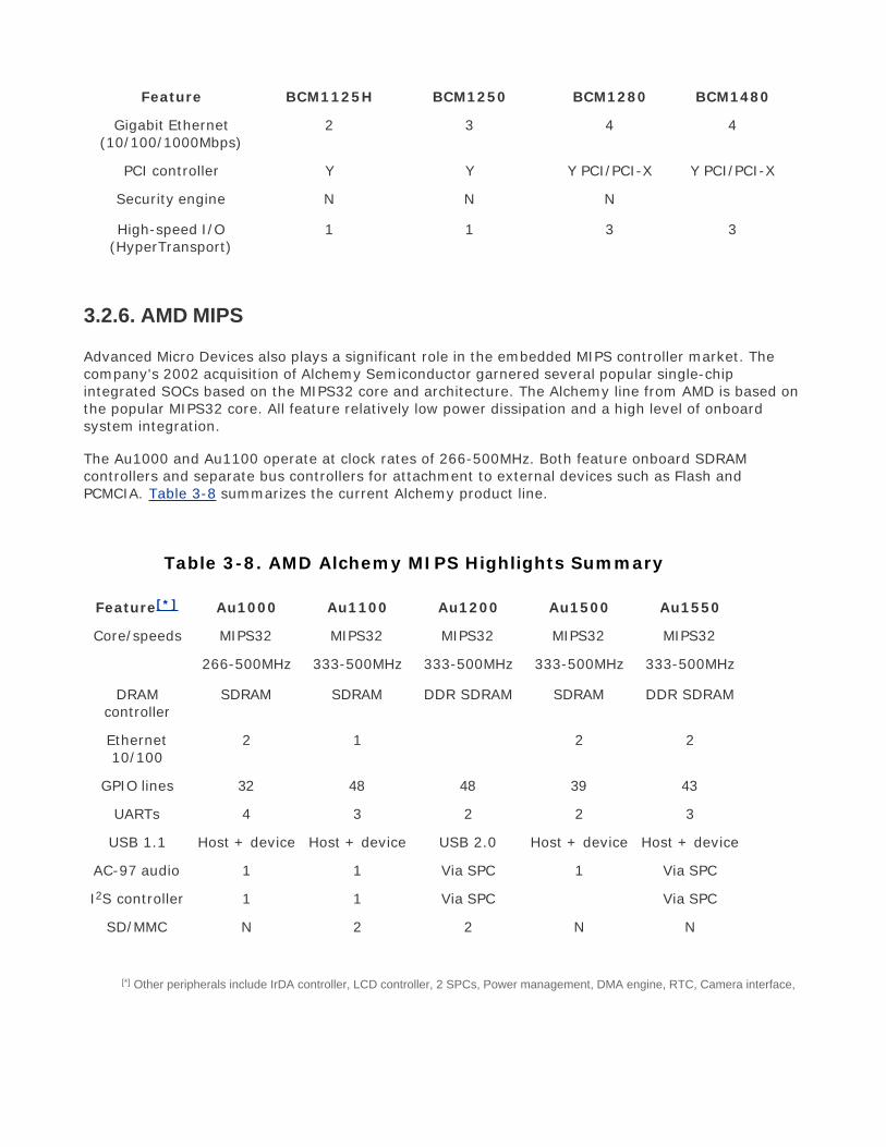
Feature BCM1125H BCM1250 BCM1280 BCM1480
Gigabit Ethernet(10/100/1000Mbps)
2 3 4 4
PCI controller Y Y Y PCI/PCI-X Y PCI/PCI-X
Security engine N N N
High-speed I/O(HyperTransport)
1 1 3 3
3.2.6. AMD MIPS
Advanced Micro Devices also plays a significant role in the embedded MIPS controller market. Thecompany's 2002 acquisition of Alchemy Semiconductor garnered several popular single-chipintegrated SOCs based on the MIPS32 core and architecture. The Alchemy line from AMD is based onthe popular MIPS32 core. All feature relatively low power dissipation and a high level of onboardsystem integration.
The Au1000 and Au1100 operate at clock rates of 266-500MHz. Both feature onboard SDRAMcontrollers and separate bus controllers for attachment to external devices such as Flash andPCMCIA. Table 3-8 summarizes the current Alchemy product line.
Table 3-8. AMD Alchemy MIPS Highlights Summary
Feature[*] Au1000 Au1100 Au1200 Au1500 Au1550
Core/speeds MIPS32 MIPS32 MIPS32 MIPS32 MIPS32
266-500MHz 333-500MHz 333-500MHz 333-500MHz 333-500MHz
DRAMcontroller
SDRAM SDRAM DDR SDRAM SDRAM DDR SDRAM
Ethernet10/100
2 1 2 2
GPIO lines 32 48 48 39 43
UARTs 4 3 2 2 3
USB 1.1 Host + device Host + device USB 2.0 Host + device Host + device
AC-97 audio 1 1 Via SPC 1 Via SPC
I2S controller 1 1 Via SPC Via SPC
SD/MMC N 2 2 N N
[*] Other peripherals include IrDA controller, LCD controller, 2 SPCs, Power management, DMA engine, RTC, Camera interface,

LCD controller, h/w hardware acceleration of encryption/decryption, PCI host controller, 4 SPCs, and Security engine.
3.2.7. Other MIPS
As we pointed out earlier, nearly 100 current MIPS licensees are shown on the MIPS Technologieslicensees web page, at www.mips.com/content/Licensees/ProductCatalog/licensees. Unfortunately, itis not possible in the space provided here to cover them all. Start your search at the MIPStechnologies website for a good cross-section of the MIPS processor vendors.
For example, ATI Technologies uses a MIPS core in its Xilleon set-top box family of chipsets. CaviumNetwork's Octeon family uses MIPS64 cores in a variety of multicore processor implementations.Integrated Device Technology, Inc., (IDT) has a family of integrated communications processorscalled Interprise, based on the MIPS architecture. PMC-Sierra, NEC, Toshiba, and others haveintegrated processors based on MIPS. All of these and more are well supported under Linux.
3.2.8. ARM
The ARM architecture has achieved a very large market share in the consumer electronicsmarketplace. Many popular and now ubiquitous products contain ARM cores. Some well-knownexamples include the Sony PlayStation Portable (PSP), Apple iPod Nano,[7] Nintendo Game Boy Microand DS, TomTom GO 300 GPS, and the Motorola E680i Mobile Phone, which features embeddedLinux. Processors containing ARM cores power a majority of the world's digital cellular phones,according to the ARM Corporate Backgrounder at www.arm.com/miscPDFs/3822.pdf.
[7] Reported by ARM to be the top-selling toy during the Christmas 2005 shopping season in the United States.
The ARM architecture is developed by ARM Holdings, plc and licensed to semiconductormanufacturers around the globe. Many of the world's leading semiconductor companies have licensedARM technology and are currently shipping integrated processors based on one of the several ARMcores.
3.2.9. TI ARM
Texas Instruments uses ARM cores in the OMAP family of integrated processors. These processorscontain many integrated peripherals intended to be used as single-chip solutions for variousconsumer products, such as cellular handsets, PDAs, and similar multimedia platforms. In addition tothe interfaces commonly found on integrated processors, such as UARTs and I2C, the OMAP devicescontain a wide range of special-purpose interfaces, including the following:
LCD screen and backlight controllers
Buzzer driver
Camera interface
MMC/SD card controller

Battery-management hardware
USB client/host interfaces
Radio modem interface logic
Integrated 2D or 3D graphics accelerators
Integrated security accelerator
S-Video outputs
IrDA controller
DACs for direct TV (PAL/NTSC) video output
Integrated DSPs for video and audio processing
Many popular cellular handsets and PDA devices have been marketed based on the TI OMAPplatform. Because they are based on an ARM core, these processors are supported by Linux today.Table 3-9 compares some of the more recent members of the TI OMAP family.
Table 3-9. TI ARM OMAP Highlights Summary
Feature OMAP1710 OMAP2420 OMAP2430 OMAP3430
Core/speeds ARM926 TEJ ARM11 ARM1136 ARM Cortex A8
Up to 200MHz 330MHz 330MHz 550MHz
DRAM controller Y Y Y Y
UARTs Y Y Y Y
USB Client + host Client + host Client + host Client + host
I2C controller Y Y Y Y
MMC-SD interface Y Y Y Y
Keypad controller Y Y Y Y
Camera interface Y Y Y Y
Graphicsaccelerator
2D 2D/3D 2D/3D Y
Integrated DSP TM320C55x TM320C55x N N
Video accelerationhardware
N Imaging VideoAccelerator (IVA)
Imaging VideoAccelerator (IVA
2)
Imaging VideoAccelerator (IVA 2
+)
Securityaccelerator
Y Y Y Y

Feature OMAP1710 OMAP2420 OMAP2430 OMAP3430
Audio codecsupport
Y Y Y Y
Bluetooth & RFmodem support
interface
Y Y Y Y
LCD controller Y Y Y Y
Display controllers N PAL/NTSCVGA/QVGA
PAL/NTSCVGA/QVGA
PAL/NTSCQVGA/XGA
3.2.10. Freescale ARM
The success of the ARM architecture is made more evident by the fact that leading manufacturers ofcompeting architectures have licensed ARM technology. As a prime example, FreescaleSemiconductor has licensed ARM technology for its line of i.MX application processors. These popularARM-based integrated processors have achieved widespread industry success in multimediaconsumer devices such as portable game platforms, PDAs, and cellular handsets.
The Freescale ARM product portfolio includes the i.MX21 and i.MX31 application processors. Thei.MX21 features an ARM9 core, and the i.MX31 has an ARM11 core. Like their TI counterparts, theseSOCs contain many integrated peripherals required by portable consumer electronics devices withmultimedia requirements. The i.MX21/31 contain some of the following integrated interfaces:
Graphics accelerator
MPEG-4 encoder
Keypad and LCD controllers
Camera interface
Audio multiplexer
IrDA infrared I/O
SD/MMC interface
Numerous external I/O, such as PCMCIA, USB, DRAM controllers, and UARTs for serial portconnection
3.2.11. Intel ARM XScale
Intel manufactures and markets several integrated processors based on the ARM v5TE architecture.Intel uses the XScale name for the architecture. These products are grouped into several applicationcategories. Table 3-10 summarizes the XScale families by application type.

Table 3-10. Intel XScale Processor Summary
Category Application Example Processors
Application processors Cellular handsets and PDAs PXA27x, PXA29x
I/O processors High-speed data processing used instorage, printing, telematics, and soon
IOP331/332/333
Network processors Networking and communications dataplane processing, fast packetprocessing, and so on
IXP425, IXP465 IXP2350,IXP2855
Many consumer and networking products have been developed using Intel XScale architectureprocessors. Some well-known examples include the GPS iQue M5 from Garmin, the iPAQ by Hewlett-Packard, smart phones from Palm (Treo) and Motorola (A760), and many others. Linux currentlysupports all these processors.
Intel's network processors are found in high-performance networking equipment where requirementsexist for fast data-path processing. Examples include deep packet inspection, dataencryption/decryption, packet filtering, and signal processing. These network processors each containan ARM core coupled with one or more dedicated processing engines, called a network processingengine (NPE). These NPEs are dedicated to specific data-path manipulation in real time at wirespeeds. The NPE is a microprocessor, in the sense that it can execute microcoded algorithms inparallel with the thread of execution in the ARM core. Refer to the Intel website, at www.intel.com,for additional information on this powerful family of integrated processors.
3.2.12. Other ARM
More than 100 semiconductor companies are developing integrated solutions based on ARMtechnologyfar too many to list here. Many offer specialized application processors serving verticalmarkets such as the handset market, storage area networking, network processing, and theautomotive market, as well as many more. These companies include Altera, PMC-Sierra, SamsungElectronics, Philips Semiconductor, Fujitsu, and more. See the ARM Technologies website atwww.arm.com for additional ARM licensees and information.
3.2.13. Other Architectures
We have covered the major architectures in widespread use in embedded Linux systems. However,for completeness, you should be aware of other architectures for which support exists in Linux. Arecent Linux snapshot revealed 25 architecture branches (subdirectories). In some instances, the 64-bit implementation of an architecture is separated from its 32-bit counterpart. In other cases, portsare not current or are no longer maintained.
The Linux source tree contains ports for Sun Sparc and Sparc64, the Xtensa from Tensilica, and the

v850 from NEC, to name a few. Spend a few minutes looking through the architecture branches ofthe Linux kernel to see the range of architectures for which Linux has been ported. Beware, however,that not all these architectures might be up-to-date in any given snapshot. You can be reasonablycertain that the major architectures are fairly current, but the only way to be certain is to follow thedevelopment in the Linux community or consult with your favorite embedded Linux vendor. AppendixE, "Open Source Resources," contains a list of resources you can consult to help you stay currentwith Linux developments.

3.3. Hardware Platforms
The idea of a common hardware reference platform is not new. The venerable PC/104 and VMEbusare two examples of hardware platforms that have withstood the test of time in the embeddedmarket.[8] More recent successful platforms include CompactPCI and its derivatives.
[8] VMEbus isn't really a hardware reference platform, per se, but based on Eurocard physical standards, the level of compatibility
among multiple vendors qualifies it for the label.
3.3.1. CompactPCI
The CompactPCI (cPCI) hardware platform is based on PCI electrical standards and Eurocard physicalspecifications. cPCI has the following general features:
Vertical cards of 3U or 6U heights
Latch system for securing and ejecting cards
Front- or rear-panel I/O connections supported
High-density backplane connector
Staggered power pins for hot-swap support
Support by many vendors
Compatibility with standard PCI chipsets
You can view highlights of and obtain specifications for the cPCI architecture at the PCI IndustrialComputer Manufacturers Group (PICMG) cPCI web page, at www.picmg.org/compactpci.stm.
3.3.2. ATCA
A successor to the successful cPCI, Advanced Telecommunications Computing Architecture is thename given to the architecture and platforms designed around the PICMG 3.x series of specifications.Many top-tier hardware manufacturers are shipping or developing new ATCA-based platforms. Theprimary applications for ATCA platforms are carrier-class telecommunications switching and transportequipment, and high-end data-center server and storage equipment.
ATCA platforms are leading the industry trend away from in-house proprietary hardware andsoftware platforms. Many of the largest equipment manufacturers in the telecommunications andnetworking markets have been slowly moving away from the custom, in-house-designed hardwareplatforms. This trend is also evident in the software platforms, from operating systems to so-calledmiddleware such as high-availability and protocol stack solutions. Downsizing and time-to-market

pressures are two key factors driving this trend.
ATCA is defined by several PICMG specifications. Table 3-11 summarizes these specifications.
Table 3-11. ATCA PICMG 3.x Specification Summary
Specification Summary
PICMG 3.0 Mechanical specifications, including interconnects, power,cooling, and base system management
PICMG 3.1 Ethernet and Fiber Channel switching fabric interface
PICMG 3.2 Infiniband switching fabric interface
PICMG 3.3 StarFabric interface
PICMG 3.4 PCI Express interface
PICMG 3.5 RapidIO Interface
The platforms described in this section are the most relevant in any discussion of embedded Linuxplatforms today. Especially with ATCA, the industry is increasingly moving toward commercial off-the-shelf (COTS) technology. Both ATCA and Linux play increasingly important roles in this industrytrend.

3.4. Chapter Summary
Many stand-alone processors are supported under Linux. The most widely supported of theseare IA32/IA64 and PowerPC architectures. These stand-alone processors are used as buildingblocks to build very-high-performance computing engines. We presented several examples fromIntel, IBM, and Freescale.
Integrated processors, or systems on chip (SOCs), dominate the embedded Linux landscape.Many vendors and several popular architectures are used in embedded Linux designs. Several ofthe most popular are presented in this chapter by architecture and manufacturer.
An increasingly popular trend is to move away from proprietary hardware and softwareplatforms, toward commercial off-the-shelf (COTS) solutions. Two popular platforms inwidespread use in embedded Linux systems: cPCI and ATCA.
3.4.1. Suggestions For Additional Reading
PowerPC 32-bit architecture reference manual:
Programming Environments Manual for 32-Bit Implementations of the PowerPC
ArchitectureRevision 2
Freescale Semiconductor, Inc.
www.freescale.com/files/product/doc/MPCFPE32B.pdf
PowerPC 64-bit architecture reference:
The Programming Environments Manual for 64-Bit MicroprocessorsVersion 3.0
International Business Machines, Inc.
Short summary of PowerPC architecture:
A Developer's Guide to the POWER Architecture
Brett Olsson, Processor Architect, IBM Corp.
Anthony Marsala, Software Engineer, IBM Corp.
www-128.ibm.com/developerworks/linux/library/l-powarch/
Intel XScale summary page
www.intel.com/design/intelxscale/


Chapter 4. The Linux KernelA DifferentPerspectiveIn this chapter
Background page 66
Linux Kernel Construction page 70
Kernel Build System page 79
Obtaining a Linux Kernel page 96
Chapter Summary page 97
If you want to learn about kernel internals, many good books are available on kernel design andoperation. Several are presented in Section 4.5.1, "Suggestions for Additional Reading," in this andother chapters throughout the book. However, very little has been written about how the kernel isorganized and structured from a project perspective. What if you're looking for the right place to addsome custom support for your new embedded project? How do you know which files are importantfor your architecture?
At first glance, it might seem an almost impossible task to understand the Linux kernel and how toconfigure it for a specific platform or application. In a recent Linux kernel snapshot, the Linux kernelsource tree consists of more than 20,000 files that contain more than six million linesand that's justthe beginning. You still need tools, a root file system, and many Linux applications to make a usablesystem.
This chapter introduces the Linux kernel and covers how the kernel is organized and how the sourcetree is structured. We then examine the components that make up the kernel image and discuss thekernel source tree layout. Following this, we present the details of the kernel build system and thefiles that drive the kernel configuration and build system. This chapter concludes by examining whatis required for a complete embedded Linux system.

4.1. Background
Linus Torvalds wrote the original version of Linux while he was a student at the University of Helsinkiin Finland. His work began in 1991. In August of that year, Linus posted this now-famousannouncement on comp.os.minix:
From: [email protected] (Linus Benedict Torvalds)Newsgroups: comp.os.minixSubject: What would you like to see most in minix?Summary: small poll for my new operating systemMessage-ID: <[email protected]>Date: 25 Aug 91 20:57:08 GMTOrganization: University of Helsinki
Hello everybody out there using minix -I'm doing a (free) operating system (just a hobby, won't be big and professionallike gnu) for 386(486) AT clones. This has been brewing since april, and isstarting to get ready. I'd like any feedback on things people like/dislike inminix, as my OS resembles it somewhat(same physical layout of the file-system(due to practical reasons)among other things).
I've currently ported bash(1.08) and gcc(1.40), and things seem to work. Thisimplies that I'll get something practical within a few months, and I'dlike toknow what features most people would want. Any suggestions are welcome, but Iwon't promise I'll implement them :-)
Linus ([email protected])
PS. Yes - it's free of any minix code, and it has a multi-threaded fs.It is NOT protable (uses 386 task switching etc), and it probably neverwill support anything other than AT-harddisks, as that's all I have :-(.
Since that initial release, Linux has matured into a full-featured operating system with robustness,reliability, and high-end features that rival those of the best commercial operating systems. By someestimates, more than half of the Internet servers on the Web are powered by Linux servers. It is nosecret that the online search giant Google uses a large collection of low-cost PCs running a fault-tolerant version of Linux to implement its popular search engine.
4.1.1. Kernel Versions
You can obtain the source code for a Linux kernel and complementary components in numerousplaces. Your local bookstore might have several versions as companion CD-ROMs in books about
Linux. You also can download the kernel itself or even complete Linux distributions from numerouslocations on the Internet. The official home for the Linux kernel is found at www.kernel.org. You willoften hear the terms mainline source or mainline kernel referring to the source trees found atkernel.org.
As this book is being written, Linux Version 2.6 is the current version. Early in the development cycle,the developers chose a numbering system designed to differentiate between kernel source treesintended for development and experimentation and source trees intended to be stable, production-ready kernels. The numbering scheme contains a major version number, a minor version number,and then a sequence number. Before Linux Version 2.6, if the minor version number is even, itdenotes a production kernel; if it is odd, it denotes a development kernel. For example:
Linux 2.4.x Production kernel
Linux 2.5.x Experimental (development)
Linux 2.6.x Production kernel
Currently, there is no separate development branch of the Linux 2.6 kernel. All new features,enhancements, and bug fixes are funneled through a series of gatekeepers who ultimately filter andpush changes up to the top-level Linux source trees maintained by Andrew Morton and LinusTorvalds.
It is easy to tell what kernel version you are working with. The first few lines of the top-levelmakefile[1] in a kernel source tree detail the exact kernel version represented by a given instance. Itlooks like this for the 2.6.14 production kernel:
[1] We talk about the kernel build system and makefiles shortly.
VERSION = 2PATCHLEVEL = 6SUBLEVEL = 14EXTRAVERSION =NAME=Affluent Albatross
Later in the same makefile, these macros are used to form a version-level macro, like this:
KERNELRELEASE=$(VERSION).$(PATCHLEVEL).$(SUBLEVEL)$(EXTRAVERSION)
This macro is used in several places in the kernel source tree to indicate the kernel version. In fact,version information is used with sufficient frequency that the kernel developers have dedicated a setof macros derived from the version macros in the makefile. These macros are found in…/include/linux/version.h[2] in the Linux kernel source tree. They are reproduced here as Listing 4-1.
[2] Throughout this book, three dots preceding any path are used to indicate whatever path it might take on your system to reach
the top-level Linux source tree.
Listing 4-1. Kernel include File:…/include/linux/version.h

#define UTS_RELEASE "2.6.14"#define LINUX_VERSION_CODE 132622#define KERNEL_VERSION(a,b,c) (((a) << 16) + ((b) << 8) + (c))
You can check the kernel version from a command prompt on a running Linux system like this:
$ cat /proc/versionLinux version 2.6.13 (chris@pluto) (gcc version 4.0.0 (DENX ELDK 4.0 4.0.0)) #2Thu Feb 16 19:30:13 EST 2006
One final note about kernel versions: You can make it easy to keep track of the kernel version in yourown kernel project by customizing the EXtrAVERSION field.
For example, if you were developing enhancements for some new kernel feature, you might setEXtrAVERSION to something like this:
EXTRAVERSION=-foo
Later, when you use cat /proc/version, you would see Linux version 2.6.13-foo, and this wouldhelp you distinguish between development versions of your own kernel.
4.1.2. Kernel Source Repositories
The official home for the kernel source code is www.kernel.org. There you can find both current andhistorical versions of the Linux kernel, as well as numerous patches. The primary FTP repositoryfound at ftp.kernel.org contains subdirectories going all the way back to Linux Version 1.0. This siteis the primary focus for the ongoing development activities within the Linux kernel.
If you download a recent Linux kernel from kernel.org, you will find files in the source tree for 25different architectures and subarchitectures. Several other development trees support the majorarchitectures. One of the reasons is simply the sheer volume of developers and changes to thekernel. If every developer on every architecture submitted patches to kernel.org, the maintainerswould be inundated with changes and patch management, and would never get to do any featuredevelopment. As anyone involved with kernel development will tell you, it's already very busy!
Several other public source trees exist outside the mainline kernel.org source, mostly forarchitecture-specific development. For example, a developer working on the MIPS architecture mightfind a suitable kernel at www.linux-mips.org. Normally, work done in an architecture tree iseventually submitted to the kernel.org kernel. Most architecture developers try to sync up to themainline kernel often, to keep up with new developments whenever possible. However, it is notalways straightforward to get one's patches included in the mainline kernel, and there will always bea lag. Indeed, differences in the architecture kernel trees exist at any given point in time.
If you are wondering how to find a kernel for your particular application, the best way to proceed isto obtain the latest stable Linux source tree. Check to see if support for your particular processorexists, and then search the Linux kernel mailing lists for any patches or issues related to your

application. Also find the mailing list that most closely matches your interest, and search that archivealso.
Appendix E, "Open Source Resources," contains several good references and sources of informationrelated to kernel source repositories, mailing lists, and more.

4.2. Linux Kernel Construction
In the next few sections, we explore the layout, organization, and construction of the Linux kernel.Armed with this knowledge, you will find it much easier to navigate this large, complex source codebase. Over time, there have been significant improvements in the organization of the source tree,especially in the architecture branch, which contains support for numerous architectures and specificmachines. As this book is being written, an effort is underway to collapse the ppc and ppc64architecture branches into a single common powerpc branch. When the dust settles, there will bemany improvements, including elimination of duplicate code, better organization of files, andpartitioning of functionality.
4.2.1. Top-Level Source Directory
We make frequent reference to the top-level source directory throughout the book. In every case, weare referring to the highest-level directory contained in the kernel source tree. On any givenmachine, it might be located anywhere, but on a desktop Linux workstation, it is often found in/usr/src/linux-x.y.z, where x.y.z represents the kernel version. Throughout the book, we use theshorthand .../ to represent the top-level kernel source directory.
The top-level kernel source directory contains the following subdirectories. (We have omitted thenondirectory entries in this listing, as well as directories used for source control for clarity andbrevity.)
arch crypto Documentation drivers fs includeinit ipc kernel lib mm netscripts security sound usr
Many of these subdirectories contain several additional levels of subdirectories containing sourcecode, makefiles, and configuration files. By far the largest branch of the Linux kernel source tree isfound under .../drivers. Here you can find support for Ethernet network cards, USB controllers, andthe numerous hardware devices that the Linux kernel supports. As you might imagine, the .../archsubdirectory is the next largest, containing support for more than 20 unique processor architectures.
Additional files found in the top-level Linux subdirectory include the top-level makefile, a hiddenconfiguration file (dot-config, introduced in Section 4.3.1, "The Dot-Config") and various otherinformational files not involved in the build itself. Finally, two important build targets are found in thetop-level kernel source tree after a successful build: System.map and the kernel proper, vmlinux. Bothare described shortly.
4.2.2. Compiling the Kernel
Understanding a large body of software such as Linux can be a daunting task. It is too large to simply

"step through" the code to follow what is happening. Multithreading and preemption add to thecomplexity of analysis. In fact, even locating the entry point (the first line of code to be executedupon entry to the kernel) can be challenging. One of the more useful ways to understand thestructure of a large binary image is to examine its built components.
The output of the kernel build system produces several common files, as well as one or morearchitecture-specific binary modules. Common files are always built regardless of the architecture.Two of the common files are System.map and vmlinux, introduced earlier. The former is useful duringkernel debug and is particularly interesting. It contains a human-readable list of the kernel symbolsand their respective addresses. The latter is an architecture-specific ELF[3] file in executable format.It is produced by the top-level kernel makefile for every architecture. If the kernel was compiled withsymbolic debug information, it will be contained in the vmlinux image. In practice, although it is anELF executable, this file is usually never booted directly, as you will see shortly.
[3] Executable and Linking Format, a de-facto standard format for binary executable files.
Listing 4-2 is a snippet of output resulting from executing make in a recent kernel tree configured forthe ARM XScale architecture. The kernel source tree was configured for the ADI Engineering Coyotereference board based on the Intel IXP425 network processor using the following command:
make ARCH=arm CROSS_COMPILE=xscale_be- ixp4xx_defconfig
This command does not build the kernel; it prepares the kernel source tree for the XScalearchitecture including an initial default configuration for this architecture and processor. It builds adefault configuration (the dot-config file) that drives the kernel build, based on the defaults found inthe ixp4xx_defconfig file. We have more to say about the configuration process later, in Section 4.3,"Kernel Build System."
Listing 4-2 shows the command that builds the kernel. Only the first few and last few lines of thebuild output are shown for this discussion.
Listing 4-2. Kernel Build Output
$ make ARCH=arm CROSS_COMPILE=xscale_be- zImage CHK include/linux/version.h HOSTCC scripts/basic/fixdep . . <hundreds of lines of output omitted here> . LD vmlinux SYSMAP System.map SYSMAP .tmp_System.map OBJCOPY arch/arm/boot/Image Kernel: arch/arm/boot/Image is ready AS arch/arm/boot/compressed/head.o GZIP arch/arm/boot/compressed/piggy.gz AS arch/arm/boot/compressed/piggy.o CC arch/arm/boot/compressed/misc.o AS arch/arm/boot/compressed/head-xscale.o AS arch/arm/boot/compressed/big-endian.o

LD arch/arm/boot/compressed/vmlinux OBJCOPY arch/arm/boot/zImage Kernel: arch/arm/boot/zImage is ready Building modules, stage 2. ...
To begin, notice the invocation of the build. Both the desired architecture (ARCH=arm) and thetoolchain (CROSS_COMPILE=xscale_be-) were specified on the command line. This forces make to usethe XScale toolchain to build the kernel image and to use the arm-specific branch of the kernel sourcetree for architecture-dependent portions of the build. We also specify a target called zImage. Thistarget is common to many architectures and is described in Chapter 5, "Kernel Initialization."
The next thing you might notice is that the actual commands used for each step have been hiddenand replaced with a shorthand notation. The motivation behind this was to clean up the build outputto draw more attention to intermediate build issues, particularly compiler warnings. In earlier kernelsource trees, each compilation or link command was output to the console verbosely, which oftenrequired several lines for each step. The end result was virtually unreadable, and compiler warningsslipped by unnoticed in the noise. The new system is definitely an improvement because any anomalyin the build process is easily spotted. If you want or need to see the complete build step, you canforce verbose output by defining V=1 on the make command line.
We have omitted most of the actual compilation and link steps in Listing 4-2, for clarity. (Thisparticular build has more than 900 individual compile and link commands in the build. That wouldhave made for a long listing, indeed.) After all the intermediate files and library archives have beenbuilt and compiled, they are put together in one large ELF build target called vmlinux. Although it isarchitecture specific, this vmlinux target is a common targetit is produced for all supported Linuxarchitectures.
4.2.3. The Kernel Proper: vmlinux
Notice this line in Listing 4-2:
LD /arch/arm/boot/compressed/vmlinux
The vmlinux file is the actual kernel proper. It is a fully stand-alone, monolithic image. No unresolvedexternal references exist within the vmlinux binary. When caused to execute in the proper context(by a bootloader designed to boot the Linux kernel), it boots the board on which it is running, leavinga completely functional kernel.
In keeping with the philosophy that to understand a system one must first understand its parts, let'slook at the construction of the vmlinux kernel object.Listing 4-3 reproduces the actual link stage ofthe build process that resulted in the vmlinux ELF object. We have formatted it with line breaks(indicated by the UNIX line-continuation character, '\') to make it more readable, but otherwise it isthe exact output produced by the vmlinux link step in the build process from Listing 4-2. If you werebuilding the kernel by hand, this is the link command you would issue from the command line.
Listing 4-3. Link Stage: vmlinux
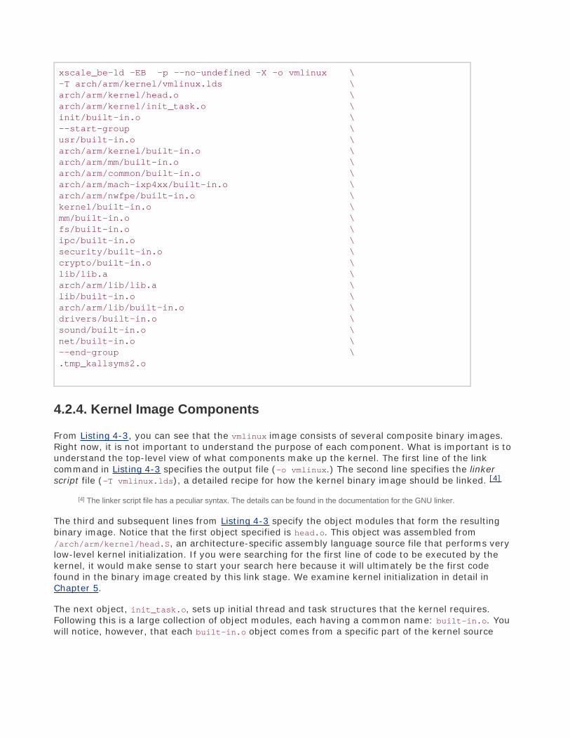
xscale_be-ld -EB -p --no-undefined -X -o vmlinux \-T arch/arm/kernel/vmlinux.lds \arch/arm/kernel/head.o \arch/arm/kernel/init_task.o \init/built-in.o \--start-group \usr/built-in.o \arch/arm/kernel/built-in.o \arch/arm/mm/built-in.o \arch/arm/common/built-in.o \arch/arm/mach-ixp4xx/built-in.o \arch/arm/nwfpe/built-in.o \kernel/built-in.o \mm/built-in.o \fs/built-in.o \ipc/built-in.o \security/built-in.o \crypto/built-in.o \lib/lib.a \arch/arm/lib/lib.a \lib/built-in.o \arch/arm/lib/built-in.o \drivers/built-in.o \sound/built-in.o \net/built-in.o \--end-group \.tmp_kallsyms2.o
4.2.4. Kernel Image Components
From Listing 4-3, you can see that the vmlinux image consists of several composite binary images.Right now, it is not important to understand the purpose of each component. What is important is tounderstand the top-level view of what components make up the kernel. The first line of the linkcommand in Listing 4-3 specifies the output file (-o vmlinux.) The second line specifies the linkerscript file (-T vmlinux.lds), a detailed recipe for how the kernel binary image should be linked. [4]
[4] The linker script file has a peculiar syntax. The details can be found in the documentation for the GNU linker.
The third and subsequent lines from Listing 4-3 specify the object modules that form the resultingbinary image. Notice that the first object specified is head.o. This object was assembled from/arch/arm/kernel/head.S, an architecture-specific assembly language source file that performs verylow-level kernel initialization. If you were searching for the first line of code to be executed by thekernel, it would make sense to start your search here because it will ultimately be the first codefound in the binary image created by this link stage. We examine kernel initialization in detail inChapter 5.
The next object, init_task.o, sets up initial thread and task structures that the kernel requires.Following this is a large collection of object modules, each having a common name: built-in.o. Youwill notice, however, that each built-in.o object comes from a specific part of the kernel source

tree, as indicated by the path component preceding the built-in.o object name. These are thebinary objects that are included in the kernel image. An illustration might make this clearer.
Figure 4-1 illustrates the binary makeup of the vmlinux image. It contains a section for each line ofthe link stage. It's not to scale because of space considerations, but you can see the relative sizes ofeach functional component.
Figure 4-1. vmlinux image components

It might come as no surprise that the three largest binary components are the file system code, thenetwork code, and all the built-in drivers. If you take the kernel code and the architecture-specifickernel code together, this is the next-largest binary component. Here you find the scheduler, processand thread management, timer management, and other core kernel functionality. Naturally, thekernel contains some architecture-specific functionality, such as low-level context switching,hardware-level interrupt and timer processing, processor exception handling, and more. This is foundin .../arch/arm/kernel.
Bear in mind that we are looking at a specific example of a kernel build. In this particular example,we are building a kernel specific to the ARM XScale architecture and, more specifically, the IntelIXP425 network processor on the ADI Engineering reference board. You can see the machine-specificbinary components in Figure 4-1 as arch/arm/mach-ixp4xx. Each architecture and machine type(processor/reference board) has different elements in the architecture-specific portions of the kernel,so the makeup of the vmlinux image is slightly different. When you understand one example, you willfind it easy to navigate others.
To help you understand the breakdown of functionality in the kernel source tree, Table 4-1 lists eachcomponent in Figure 4-1, together with a short description of each binary element that makes up thevmlinux image.
Table 4-1. vmlinux Image Components Description
Component Description
arch/arm/kernel/head.o Kernel architecture-specific startup code.
init_task.o Initial thread and task structs required by kernel.
init/built-in.o Main kernel-initialization code. See Chapter 5.
usr/built-in.o Built-in initramfs image. See Chapter 5.
arch/arm/kernel/built-in.o Architecture-specific kernel code.
arch/arm/mm/built-in.o Architecture-specific memory-management code.
arch/arm/common/built-in.o Architecture-specific generic code. Varies byarchitecture.
arch/arm/mach-ixp4xx/built-in.o Machine-specific code, usually initialization.
arch/arm/nwfpe/built-in.o Architecture-specific floating point-emulation code.
kernel/built-in.o Common components of the kernel itself.
mm/built-in.o Common components of memory-management code.
ipc/built-in.o Interprocess communications, such as SysV IPC.
security/built-in.o Linux security components.
lib/lib.a Archive of miscellaneous helper functions.
arch/arm/lib/lib.a Architecture-specific common facilities. Varies byarchitecture.

Component Description
lib/built-in.o Common kernel helper functions.
drivers/built-in.o All the built-in driversnot loadable modules.
sound/built-in.o Sound drivers.
net/built-in.o Linux networking.
.tmp_kallsyms2.o Symbol table.
When we speak of the kernel proper, this vmlinux image is being referenced. As mentioned earlier,very few platforms boot this image directly. For one thing, it is almost universally compressed. At abare minimum, a bootloader must decompress the image. Many platforms require some type of stubbolted onto the image to perform the decompression. Later in Chapter 5, you will learn how thisimage is packaged for different architectures, machine types, and bootloaders, and the requirementsfor booting it.
4.2.5. Subdirectory Layout
Now that you've seen how the build system controls the kernel image, let's take a look at arepresentative kernel subdirectory. Listing 4-4 details the contents of the mach-ixp425 subdirectory.This directory exists under the .../arch/arm architecture-specific branch of the source tree.
Listing 4-4. Kernel Subdirectory
$ ls -l linux-2.6/arch/arm/mach-ixp425total 92-rw-rw-r-- 1 chris chris 11892 Oct 10 14:53 built-in.o-rw-rw-r-- 1 chris chris 6924 Sep 29 15:39 common.c-rw-rw-r-- 1 chris chris 3525 Oct 10 14:53 common.o-rw-rw-r-- 1 chris chris 13062 Sep 29 15:39 common-pci.c-rw-rw-r-- 1 chris chris 7504 Oct 10 14:53 common-pci.o-rw-rw-r-- 1 chris chris 1728 Sep 29 15:39 coyote-pci.c-rw-rw-r-- 1 chris chris 1572 Oct 10 14:53 coyote-pci.o-rw-rw-r-- 1 chris chris 2118 Sep 29 15:39 coyote-setup.c-rw-rw-r-- 1 chris chris 2180 Oct 10 14:53 coyote-setup.o-rw-rw-r-- 1 chris chris 2042 Sep 29 15:39 ixdp425-pci.c-rw-rw-r-- 1 chris chris 3656 Sep 29 15:39 ixdp425-setup.c-rw-rw-r-- 1 chris chris 2761 Sep 29 15:39 Kconfig-rw-rw-r-- 1 chris chris 259 Sep 29 15:39 Makefile-rw-rw-r-- 1 chris chris 3102 Sep 29 15:39 prpmc1100-pci.c
The directory contents in Listing 4-4 have common components found in many kernel sourcesubdirectories: Makefile and Kconfig. These two files drive the kernel configuration-and-buildprocess. Let's look at how that works.


4.3. Kernel Build System
The Linux kernel configuration and build system is rather complicated, as one would expect ofsoftware projects containing more than six million lines of code! In this section, we cover thefoundation of the kernel build system for developers who need to customize the build environment.
A recent Linux kernel snapshot showed more than 800 makefiles[5] in the kernel source tree. Thismight sound like a large number, but it might not seem so large when you understand the structureand operation of the build system. The Linux kernel build system has been significantly updated sincethe days of Linux 2.4 and earlier. For those of you familiar with the older kernel build system, we'resure you will find the new Kbuild system to be a huge improvement. We limit our discussion in thissection to this and later kernel versions based on Kbuild.
[5] Not all these makefiles are directly involved in building the kernel. Some, for example, build documentation files.
4.3.1. The Dot-Config
Introduced earlier, the dot-config file is the configuration blueprint for building a Linux kernel image.You will likely spend significant effort at the start of your Linux project building a configuration that isappropriate for your embedded platform. Several editors, both text based and graphical, aredesigned to edit your kernel configuration. The output of this configuration exercise is written to aconfiguration file named .config, located in the top-level Linux source directory that drives the kernelbuild.
You have likely invested significant time perfecting your kernel configuration, so you will want toprotect it. Several make commands delete this configuration file without warning. The most common ismake mrproper. This make target is designed to return the kernel source tree to its pristine,unconfigured state. This includes removing all configuration data from the source treeand, yes, itdeletes your .config.
As you might know, any filename in Linux preceded by a dot is a hidden file in Linux. It is unfortunatethat such an important file is marked hidden; this has brought considerable grief to more than onedeveloper. If you execute make mrproper without having a backup copy of your .config file, you, too,will share our grief. (You have been warnedback up your .config file!)
The .config file is a collection of definitions with a simple format. Listing 4.5 shows a snippet of a.config from a recent Linux kernel release.
Listing 4-5. Snippet from Linux 2.6 .config

...# USB support#CONFIG_USB=m# CONFIG_USB_DEBUG is not set
# Miscellaneous USB options#CONFIG_USB_DEVICEFS=y# CONFIG_USB_BANDWIDTH is not set# CONFIG_USB_DYNAMIC_MINORS is not set
# USB Host Controller Drivers#CONFIG_USB_EHCI_HCD=m# CONFIG_USB_EHCI_SPLIT_ISO is not set# CONFIG_USB_EHCI_ROOT_HUB_TT is not setCONFIG_USB_OHCI_HCD=mCONFIG_USB_UHCI_HCD=m...
To understand the .config file, you need to understand a fundamental aspect of the Linux kernel.Linux has a monolithic structure. That is, the entire kernel is compiled and linked as a single staticallylinked executable. However, it is possible to compile and incrementally link[6] a set of sources into asingle object module suitable for dynamic insertion into a running kernel. This is the usual method forsupporting most common device drivers. In Linux, these are called loadable modules. They are alsogenerically called device drivers. After the kernel is booted, a special application program is invokedto insert the loadable module into a running kernel.
[6] Incremental linking is a technique used to generate an object module that is intended to be linked again into another object. In
this way, unresolved symbols that remain after incremental linking do not generate errorsthey are resolved at the next link stage.
Armed with that knowledge, let's look again at Listing 4-5. This snippet of the configuration file(.config) shows a portion of the USB subsystem configuration. The first configuration option,CONFIG_USB=m, declares that the USB subsystem is to be included in this kernel configuration and thatit will be compiled as a dynamically loadable module(=m), to be loaded sometime after the kernel hasbooted. The other choice would have been =y, in which case the USB module would be compiled andstatically linked as part of the kernel image itself. It would end up in the .../drivers/built-in.ocomposite binary that you saw in Listing 4-3 and Figure 4-1. The astute reader will realize that if adriver is configured as a loadable module, its code is not included in the kernel proper, but ratherexists as a stand-alone object module, a loadable module, to be inserted into the running kernel afterboot.
Notice in Listing 4-5 the CONFIG_USB_DEVICEFS=y declaration. This configuration option behaves in aslightly different manner. In this case, USB_DEVICEFS (as configuration options are commonlyabbreviated) is not a stand-alone module, but rather a feature to be enabled or disabled in the USBdriver. It does not necessarily result in a module that is compiled into the kernel proper (=y); instead,it enables one or more features, often represented as additional object modules to be included in theoverall USB device driver module. Usually, the help text in the configuration editor, or the hierarchypresented by the configuration editor, makes this distinction clear.

4.3.2. Configuration Editor(s)
Early kernels used a simple command line driven script to configure the kernel. This was cumbersomeeven for early kernels, in which the number of configuration parameters was much smaller. Thiscommand line style interface is still supported, but using it is tedious, to say the least. A typicalconfiguration from a recent kernel requires answering more than 600 questions from the commandline, entering your choice followed by the Enter key for each query from the script. Furthermore, ifyou make a mistake, there is no way to back up; you must start from the beginning again. That canbe profoundly frustrating if you make a mistake on the 599th entry!
In some situations, such as building a kernel on an embedded system without graphics, using thecommand line configuration utility is unavoidable, but this author would go to great lengths to find away around it.
The kernel-configuration subsystem uses several graphical front ends. In fact, a recent Linux kernelrelease included 10 such configuration targets. They are summarized here, from text taken directlyfrom the output of make help:
config Update current config using a line-oriented program
menuconfig Update current config using a menu-based program
xconfig Update current config using a QT-based front end
gconfig Update current config using a GTK-based front end
oldconfig Update current config using a provided .config as the base
randconfig New config with random answer to all options
defconfig New config with default answer to all options
allmodconfig New config that selects modules, when possible
allyesconfig New config in which all options are accepted with yes
allnoconfig New minimal config
The first four of these makefile configuration targets invoke a form of configuration editor, asdescribed in the list. Because of space considerations, we focus our discussion in this chapter andothers only on the GTK-based graphical front end. Realize that you can use the configuration editor ofyour choice with the same results.
The configuration editor is invoked by entering the command make gconfig from the top-level kerneldirectory.[7] Figure 4-2 shows the top-level configuration menu presented to the developer whengconfig is run. From here, every available configuration parameter can be accessed to generate acustom kernel configuration.
[7] As mentioned, you can use the configuration editor of your choice, such as make xconfig or make menuconfig.

Figure 4-2. Top-level kernel configuration
[View full size image]
When the configuration editor is exited, you are prompted to save your changes. If you elect to saveyour changes, the global configuration file .config is updated (or created, if it does not alreadyexist). This .config file, introduced earlier, drives the kernel build via the top-level makefile. You willnotice in this makefile that the .config file is read directly by an include statement.
Most kernel software modules also read the configuration indirectly via the .config file as follows.During the build process, the .config file is processed into a C header file found in the.../include/linux directory, called autoconf.h. This is an automatically generated file and shouldnever be edited directly because edits are lost each time a configuration editor is run. Many kernelsource files include this file directly using the #include preprocessor directive. Listing 4-6 reproducesa section of this header file that corresponds to the earlier USB example above. Note that, for eachentry in the .config file snippet in Listing 4-5, a corresponding entry is created in autoconf.h. This ishow the source files in the kernel source tree reference the kernel configuration.
Listing 4-6. Linux autoconf.h

/* * USB support */#define CONFIG_USB_MODULE 1#undef CONFIG_USB_DEBUG
/* * Miscellaneous USB options */#define CONFIG_USB_DEVICEFS 1#undef CONFIG_USB_BANDWIDTH#undef CONFIG_USB_DYNAMIC_MINORS
/* * USB Host Controller Drivers */#define CONFIG_USB_EHCI_HCD_MODULE 1#undef CONFIG_USB_EHCI_SPLIT_ISO#undef CONFIG_USB_EHCI_ROOT_HUB_TT#define CONFIG_USB_OHCI_HCD_MODULE 1#define CONFIG_USB_UHCI_HCD_MODULE 1
If you haven't already done so, execute make gconfig in your top-level kernel source directory, andpoke around this configuration utility to see the large number of subsections and configurationoptions available to the Linux developer. As long as you don't explicitly save your changes, they arelost upon exiting the configuration editor and you can safely explore without modifying your kernelconfiguration.[8] Many configuration parameters contain helpful explanation text, which can add toyour understanding of the different configuration options.
[8] Better yet, make a backup copy of your .config file.
4.3.3. Makefile Targets
If you type make help at the top-level Linux source directory, you are presented with a list of targetsthat can be generated from the source tree. The most common use of make is to specify no target.This generates the kernel ELF file vmlinux and is the default binary image for your chosenarchitecture (for example, bzImage for x86). Specifying make with no target also builds all the device-driver modules (kernel-loadable modules) specified by the configuration.
Many architectures and machine types require binary targets specific to the architecture andbootloader in use. One of the more common architecture specific targets is zImage. In manyarchitectures, this is the default target image that can be loaded and run on the target embeddedsystem. One of the common mistakes that newcomers make is to specify bzImage as the make target.The bzImage target is specific to the x86/PC architecture. Contrary to popular myth, the bzImage isnot a bzip2-compressed image. It is a big zImage. Without going into the details of legacy PCarchitecture, it is enough to know that a bzImage is suitable only for PC-compatible machines with anindustry-standard PC-style BIOS.
Listing 4-7 contains the output from make help from a recent Linux kernel. You can see from the

listing that many targets are available in the top-level Linux kernel makefile. Each is listed along witha short description of its use. It is important to realize that even the help make target (as in makehelp) is architecture specific. You get a different list of architecture-specific targets depending on thearchitecture you pass on the make invocation. Listing 4-7 illustrates an invocation that specifies theARM architecture, as you can see from the make command line.
Listing 4-7. Makefile Targets
$ make ARCH=arm helpCleaning targets: clean - remove most generated files but keep the config mrproper - remove all generated files + config + various backup files
Configuration targets: config - Update current config utilising a line-oriented program menuconfig - Update current config utilising a menu based program xconfig - Update current config utilising a QT based front-end gconfig - Update current config utilising a GTK based front-end oldconfig - Update current config utilising a provided .config as base randconfig - New config with random answer to all options defconfig - New config with default answer to all options allmodconfig - New config selecting modules when possible allyesconfig - New config where all options are accepted with yes allnoconfig - New minimal config
Other generic targets: all - Build all targets marked with [*]* vmlinux - Build the bare kernel* modules - Build all modules modules_install - Install all modules dir/ - Build all files in dir and below dir/file.[ois] - Build specified target only dir/file.ko - Build module including final link rpm - Build a kernel as an RPM package tags/TAGS - Generate tags file for editors cscope - Generate cscope index kernelrelease - Output the release version string
Static analysers buildcheck - List dangling references to vmlinux discarded sections and init sections from non-init sections checkstack - Generate a list of stack hogs namespacecheck - Name space analysis on compiled kernel
Kernel packaging: rpm-pkg - Build the kernel as an RPM package binrpm-pkg - Build an rpm package containing the compiled kernel and modulesdeb-pkg - Build the kernel as an deb package tar-pkg - Build the kernel as an uncompressed tarball

targz-pkg - Build the kernel as a gzip compressed tarball tarbz2-pkg - Build the kernel as a bzip2 compressed tarball
Documentation targets: Linux kernel internal documentation in different formats: xmldocs (XML DocBook), psdocs (Postscript), pdfdocs (PDF) htmldocs (HTML), mandocs (man pages, use installmandocs to install)
Architecture specific targets (arm):* zImage - Compressed kernel image (arch/arm/boot/zImage) Image - Uncompressed kernel image (arch/arm/boot/Image)* xipImage - XIP kernel image, if configured (arch/arm/boot/xipImage) bootpImage - Combined zImage and initial RAM disk (supply initrd image via make variable INITRD=<path>) install - Install uncompressed kernel zinstall - Install compressed kernel Install using (your) ~/bin/installkernel or (distribution) /sbin/installkernel or install to $(INSTALL_PATH) and run lilo assabet_defconfig - Build for assabet badge4_defconfig - Build for badge4 bast_defconfig - Build for bast cerfcube_defconfig - Build for cerfcube clps7500_defconfig - Build for clps7500 collie_defconfig - Build for collie corgi_defconfig - Build for corgi ebsa110_defconfig - Build for ebsa110 edb7211_defconfig - Build for edb7211 enp2611_defconfig - Build for enp2611 ep80219_defconfig - Build for ep80219 epxa10db_defconfig - Build for epxa10db footbridge_defconfig - Build for footbridge fortunet_defconfig - Build for fortunet h3600_defconfig - Build for h3600 h7201_defconfig - Build for h7201 h7202_defconfig - Build for h7202 hackkit_defconfig - Build for hackkit integrator_defconfig - Build for integrator iq31244_defconfig - Build for iq31244 iq80321_defconfig - Build for iq80321 iq80331_defconfig - Build for iq80331 iq80332_defconfig - Build for iq80332 ixdp2400_defconfig - Build for ixdp2400 ixdp2401_defconfig - Build for ixdp2401 ixdp2800_defconfig - Build for ixdp2800 ixdp2801_defconfig - Build for ixdp2801 ixp4xx_defconfig - Build for ixp4xx jornada720_defconfig - Build for jornada720 lart_defconfig - Build for lart lpd7a400_defconfig - Build for lpd7a400 lpd7a404_defconfig - Build for lpd7a404

lubbock_defconfig - Build for lubbocklusl7200_defconfig - Build for lusl7200 mainstone_defconfig - Build for mainstone mx1ads_defconfig - Build for mx1ads neponset_defconfig - Build for neponset netwinder_defconfig - Build for netwinder omap_h2_1610_defconfig - Build for omap_h2_1610 pleb_defconfig - Build for pleb poodle_defconfig - Build for poodle pxa255-idp_defconfig - Build for pxa255-idp rpc_defconfig - Build for rpc s3c2410_defconfig - Build for s3c2410 shannon_defconfig - Build for shannon shark_defconfig - Build for shark simpad_defconfig - Build for simpad smdk2410_defconfig - Build for smdk2410 spitz_defconfig - Build for spitz versatile_defconfig - Build for versatile
make V=0|1 [targets] 0 => quiet build (default), 1 => verbose build make O=dir [targets] Locate all output files in "dir", including .config make C=1 [targets] Check all c source with $CHECK (sparse) make C=2 [targets] Force check of all c source with $CHECK (sparse)
Execute "make" or "make all" to build all targets marked with [*]For further info see the ./README file
Many of these targets you might never use. However, it is useful to know that they exist. As you cansee from Listing 4-7, the targets listed with an asterisk are built by default. Notice the numerousdefault configurations, listed as *_defconfig. Recall from Section 4.2.2, "Compiling the Kernel," thecommand we used to preconfigure a pristine kernel source tree: We invoked make with anarchitecture and a default configuration. The default configuration was ixp4xx_defconfig, whichappears in this list of ARM targets. This is a good way to discover all the default configurationsavailable for a particular kernel release and architecture.
4.3.4. Kernel Configuration
Kconfig (or a file with a similar root followed by an extension, such as Kconfig.ext) exists in almost300 kernel subdirectories. Kconfig drives the configuration process for the features contained withinits subdirectory. The contents of Kconfig are parsed by the configuration subsystem, which presentsconfiguration choices to the user, and contains help text associated with a given configurationparameter.
The configuration utility (such as gconf, presented earlier) reads the Kconfig files starting from thearch subdirectory's Kconfig file. It is invoked from the Kconfig makefile with an entry that looks likethis:
gconfig: $(obj)/gconf

$< arch/$(ARCH)/Kconfig
Depending on which architecture you are building, gconf reads this architecture-specific Kconfig asthe top-level configuration definition. Contained within Kconfig are a number of lines that look likethis:
source "drivers/pci/Kconfig"
This directive tells the configuration editor utility to read in another Kconfig file from another locationwithin the kernel source tree. Each architecture contains many such Kconfig files; taken together,these determine the complete set of menu options presented to the user when configuring the kernel.Each Kconfig file is free to source additional Kconfig files in different parts of the source tree. Theconfiguration utilitygconf, in this case, recursively reads the Kconfig file chain and builds theconfiguration menu structure.
Listing 4-8 is a partial tree view of the Kconfig files associated with the ARM architecture. In a recentLinux 2.6 source tree from which this example was taken, the kernel configuration was defined by170 separate Kconfig files. This listing omits most of those, for the sake of space and claritythe ideais to show the overall structure. To list them all in this tree view would take several pages of thistext.
Listing 4-8. Partial Listing of Kconfig for ARM Architecture
arch/arm/Kconfig <<<<<< (top level Kconfig)|-> init/Kconfig| ...|-> arch/arm/mach-iop3xx/Kconfig|-> arch/arm/mach-ixp4xx/Kconfig| ...|-> net/Kconfig| |-> net/ipv4/Kconfig| | |-> net/ipv4/ipvs/Kconfig| ...|-> drivers/char/Kconfig| |-> drivers/serial/Kconfig| ...|-> drivers/usb/Kconfig| |-> drivers/usb/core/Kconfig| |-> drivers/usb/host/Kconfig| ...|-> lib/Kconfig
Looking at Listing 4-8, the file arch/arm/Kconfig would contain a line like this:
source "net/Kconfig"

The file net/Kconfig would contain a line like this:
source "net/ipv4/Kconfig"
…and so on.
As mentioned earlier, these Kconfig files taken together determine the configuration menu structureand configuration options presented to the user during kernel configuration. Figure 4-3 is an exampleof the configuration utility (gconf) for the ARM architecture compiled from the example in Listing 4-8.
Figure 4-3. gconf configuration screen
[View full size image]
4.3.5. Custom Configuration Options
Many embedded developers add feature support to the Linux kernel to support their particularcustom hardware. One of the most common examples of this is multiple versions of a given hardwareplatform, each of which requires some compile-time options to be configured in the kernel sourcetree. Instead of having a separate version of the kernel source tree for each hardware version, adeveloper can add configuration options to enable his custom features.
The configuration management architecture described in the previous paragraphs makes it easy to

customize and add features. A quick peek into a typical Kconfig file shows the structure of theconfiguration script language. As an example, assume that you have two hardware platforms basedon the IXP425 network processor, and that your engineering team had dubbed them Vega andConstellation. Each board has specialized hardware that must be initialized early during the kernelboot phase. Let's see how easy it is to add these configuration options to the set of choices presentedto the developer during kernel configuration. Listing 4-9 is a snippet from the top-level ARM Kconfigfile.
Listing 4-9. Snippet from …/arch/arm/Kconfig
source "init/Kconfig"
menu "System Type"
choice prompt "ARM system type" default ARCH_RPC
config ARCH_CLPS7500 bool "Cirrus-CL-PS7500FE"
config ARCH_CLPS711X bool "CLPS711x/EP721x-based"
...
source "arch/arm/mach-ixp4xx/Kconfig
In this Kconfig snippet taken from the top-level ARM architecture Kconfig, you see the menu itemSystem Type being defined. After the ARM System type prompt, you see a list of choices related to theARM architecture. Later in the file, you see the inclusion of the IXP4xx-specific Kconfig definitions. Inthis file, you add your custom configuration switches. Listing 4-10 reproduces a snippet of this file.Again, for readability and convenience, we've omitted irrelevant text, as indicated by the ellipsis.
Listing 4-10. File Snippet: arch/arm/mach-ixp4xx/Kconfig

menu "Intel IXP4xx Implementation Options"
comment "IXP4xx Platforms"
config ARCH_AVILA bool "Avila" help Say 'Y' here if you want your kernel to support...
config ARCH_ADI_COYOTE bool "Coyote" help Say 'Y' here if you want your kernel to support the ADI Engineering Coyote...
# (These are our new custom options) config ARCH_VEGA bool "Vega" help Select this option for "Vega" hardware support
config ARCH_CONSTELLATION bool "Constellation" help Select this option for "Constellation" hardware support ...
Figure 4-4 illustrates the result of these changes as it appears when running the gconf utility (viamake ARCH=arm gconfig). As a result of these simple changes, the configuration editor now includesoptions for our two new hardware platforms.[9] Shortly, you'll see how you can use this configurationinformation in the source tree to conditionally select objects that contain support for your newboards.
[9] We have intentionally removed many options under ARM system type and Intel IXP4 xx Implementation Options to fit the
picture on the page.
Figure 4-4. Custom configuration options
[View full size image]

After the configuration editor (gconf, in these examples) is run and you select support for one of yourcustom hardware platforms, the .config file introduced earlier contains macros for your new options.As with all kernel-configuration options, each is preceded with CONFIG_ to identify it as a kernel-configuration option. As a result, two new configuration options have been defined, and their statehas been recorded in the .config file. Listing 4-11 shows the new .config file with your newconfiguration options.
Listing 4-11. Customized .config File Snippet
...## IXP4xx Platforms## CONFIG_ARCH_AVILA is not set# CONFIG_ARCH_ADI_COYOTE is not setCONFIG_ARCH_VEGA=y# CONFIG_ARCH_CONSTELLATION is not set# CONFIG_ARCH_IXDP425 is not set# CONFIG_ARCH_PRPMC1100 is not set...
Notice two new configuration options related to your Vega and Constellation hardware platforms. Asillustrated in Figure 4-4, you selected support for Vega; in the .config file, you can see the newCONFIG_ option representing that the Vega board is selected and set to the value 'y'. Notice also that

the CONFIG_ option related to Constellation is present but not selected.
4.3.6. Kernel Makefiles
When building the kernel, the Makefiles scan the configuration and decide what subdirectories todescend into and what source files to compile for a given configuration. To complete the example ofadding support for two custom hardware platforms, Vega and Constellation, let's look at the makefilethat would read this configuration and take some action based on customizations.
Because you're dealing with hardware specific options in this example, assume that thecustomizations are represented by two hardware-setup modules called vega_setup.c andconstellation_setup.c. We've placed these C source files in the .../arch/arm/mach-ixp4xxsubdirectory of the kernel source tree. Listing 4-12 contains the complete makefile for this directoryfrom a recent Linux release.
Listing 4-12. Makefile from …/arch/arm/mach-ixp4xx KernelSubdirectory
## Makefile for the linux kernel.#
obj-y += common.o common-pci.o
obj-$(CONFIG_ARCH_IXDP4XX) += ixdp425-pci.o ixdp425-setup.oobj-$(CONFIG_MACH_IXDPG425) += ixdpg425-pci.o coyote-setup.oobj-$(CONFIG_ARCH_ADI_COYOTE) += coyote-pci.o coyote-setup.oobj-$(CONFIG_MACH_GTWX5715) += gtwx5715-pci.o gtwx5715-setup.o
You might be surprised by the simplicity of this makefile. Much work has gone into the developmentof the kernel build system for just this reason. For the average developer who simply needs to addsupport for his custom hardware, the design of the kernel build system makes these kinds ofcustomizations very straightforward.[10]
[10] In actuality, the kernel build system is very complicated, but most of the complexity is cleverly hidden from the average
developer. As a result, it is relatively easy to add, modify, or delete configurations without having to be an expert.
Looking at this makefile, it might be obvious what must be done to introduce new hardware setuproutines conditionally based on your configuration options. Simply add the following two lines at thebottom of the makefile, and you're done:
obj-$(CONFIG_ARCH_VEGA) += vega_setup.oobj-$(CONFIG_ARCH_CONSTELLATION) += costellation_setup.o
These steps complete the simple addition of setup modules specific to the hypothetical example

custom hardware. Using similar logic, you should now be able to make your own modifications to thekernel configuration/build system.
4.3.7. Kernel Documentation
A wealth of information is available in the Linux source tree itself. It would be difficult indeed to readit all because there are nearly 650 documentation files in 42 subdirectories in the .../Documentationdirectory. Be cautious in reading this material: Given the rapid pace of kernel development andrelease, this documentation tends to become outdated quickly. Nonetheless, it often provides a greatstarting point from which you can form a foundation on a particular kernel subsystem or concept.
Do not neglect the Linux Documentation Project, found at www.tldp.org, where you might find themost up-to-date version of a particular document or man page.[11] The list of suggested reading atthe end of this chapter duplicates the URL for the Linux Documentation Project, for easy reference. Ofparticular interest to the previous discussion is the Kbuild documentation found in the kernel.../Documentation/kbuild subdirectory.
[11] Always assume that features advance faster than the corresponding documentation, so treat the docs as a guide rather than
indisputable facts.
No discussion of Kernel documentation would be complete without mentioning Google. One day soon,Googling will appear in Merriam Webster's as a verb! Chances are, many problems and questions youmight ask have already been asked and answered before. Spend some time to become proficient insearching the Internet for answers to questions. You will discover numerous mailing lists and otherinformation repositories full of useful information related to your specific project or problem.Appendix E contains a useful list of open-source resources.

4.4. Obtaining a Linux Kernel
In general, you can obtain an embedded Linux kernel for your hardware platform in three ways: Youcan purchase a suitable commercial embedded Linux distribution; you can download a free embeddeddistribution, if you can find one suitable for your particular architecture and processor; or you canfind the closest open-source Linux kernel to your application and port it yourself. We discuss Linuxporting in Chapter 16, "Porting Linux."
Although porting an open source kernel to your custom board is not necessarily difficult, it representsa significant investment in engineering/development resources. This approach gives you access tofree software, but deploying Linux in your development project is far from free, as we discussed inChapter 1, "Introduction." Even for a small system with minimal application requirements, you needmany more components than just a Linux kernel.
4.4.1. What Else Do I Need?
This chapter has focused on the layout and construction of the Linux kernel itself. As you might havealready discovered, Linux is only a small component of an embedded system based on Linux. Inaddition to the Linux kernel, you need the following components to develop, test, and launch yourembedded Linux widget:
Bootloader ported to and configured for your specific hardware platform
Cross-compiler and associated toolchain for your chosen architecture
File system containing many packagesbinary executables and libraries compiled for your nativehardware architecture/processor
Device drivers for any custom devices on your board
Development environment, including host tools and utilities
Linux kernel source tree enabled for your particular processor and board
These are the components of an embedded Linux distribution.

4.5. Chapter Summary
The Linux kernel is more than 10 years old and has become a mainstream, well-supportedoperating system for many architectures.
The Linux open source home is found at www.kernel.org. Virtually every release version of thekernel is available there, going all the way back to Linux 1.0.
We leave it to other great books to describe the theory and operation of the Linux kernel. Herewe discussed how it is built and identified the components that make up the image. Breaking upthe kernel into understandable pieces is the key to learning how to navigate this large softwareproject.
This chapter covered the kernel build system and the process of modifying the build system tofacilitate modifications.
Several kernel configuration editors exist. We chose one and examined how it is driven and howto modify the menus and menu items within. These concepts apply to all the graphical frontends.
The kernel itself comes with an entire directory structure full of useful kernel documentation.This is a helpful resource for understanding and navigating the kernel and its operation.
This chapter concluded with a brief introduction to the options available for obtaining anembedded Linux distribution.
4.5.1. Suggestions for Additional Reading
Linux Kernel HOWTO:www.tldp.org/HOWTO/Kernel-HOWTO
Kernel Kbuild documentation:http://sourceforge.net/projects/kbuild/
The Linux Documentation Project:www.tldp.org/
Tool Interface Standard (TIS) Executable and Linking Format (ELF) Specification,Version 1.2TIS Committee, May 1995
Linux kernel source tree:…/Documentation/kbuild/makefiles.txt
Linux kernel source tree:…/Documentation/kbuild/kconfig-language.txt

Linux Kernel Development, 2nd EditionRovert LoveNovell Press, 2005

Chapter 5. Kernel InitializationIn this chapter
Composite Kernel Image: Piggy and Friends page 100
Initialization Flow of Control page 109
Kernel Command Line Processing page 114
Subsystem Initialization page 121
The init Thread page 123
Chapter Summary page 128
When the power is applied to an embedded Linux system, a complex sequence of events is started.After a few seconds, the Linux kernel is operational and has spawned a series of application programsas specified by the system init scripts. A significant portion of these activities are governed by systemconfiguration and are under the control of the embedded developer.
This chapter examines the initial sequence of events in the Linux kernel. We take a detailed look atthe mechanisms and processes used during kernel initialization. We describe the Linux kernelcommand line and its use to customize the Linux environment on startup. With this knowledge, youwill be able to customize and control the initialization sequence to meet the requirements of yourparticular embedded system.

5.1. Composite Kernel Image: Piggy and Friends
At power-on, the bootloader in an embedded system is first to get processor control. After thebootloader has performed some low-level hardware initialization, control is passed to the Linuxkernel. This can be a manual sequence of events to facilitate the development process (for example,the user types interactive load/boot commands at the bootloader prompt), or an automated startupsequence typical of a production environment. We have dedicated Chapter 7 , "Bootloaders," to thissubject, so we defer any detailed bootloader discussion to that chapter.
In Chapter 4 , "The Linux Kernel: A Different Perspective," we examined the components that makeup the Linux kernel image. Recall that one of the common files built for every architecture is the ELFbinary named vmlinux . This binary file is the monolithic kernel itself, or what we have been callingthe kernel proper . In fact, when we looked at its construction in the link stage of vmlinux , wepointed out where we might look to see where the first line of code might be found. In mostarchitectures, it is found in an assembly language source file called head.S or similar. In the PowerPC(ppc ) branch of the kernel, several versions of head.S are present, depending on the processor. Forexample, the AMCC 440 series processors are initialized from a file called head_44x.S .
Some architectures and bootloaders are capable of directly booting the vmlinux kernel image. Forexample, platforms based on PowerPC architecture and the U-Boot bootloader can usually boot thevmlinux image directly[1] (after conversion from ELF to binary, as you will shortly see). In othercombinations of architecture and bootloader, additional functionality might be needed to set up theproper context and provide the necessary utilities for loading and booting the kernel.
[1] The kernel image is nearly always stored in compressed format, unless boot time is a critical issue. In this case, the image
might be called uImage, a compressed vmlinux file with a U-Boot header. See Chapter 7 ,"Bootloaders."
Listing 5-1 details the final sequence of steps in the kernel build process for a hardware platformbased on the ADI Engineering Coyote Reference Platform, which contains an Intel IXP425 networkprocessor. This listing uses the quiet form of output from the kernel build system, which is thedefault. As pointed out in Chapter 4 , it is a useful shorthand notation, allowing more focus on errorsand warnings during the build.
Listing 5-1. Final Kernel Build Sequence: ARM/IXP425 (Coyote)
$ make ARCH=arm CROSS_COMPILE=xscale_be- zImage
... < many build steps omitted for clarity> LD vmlinux SYSMAP System.map OBJCOPY arch/arm/boot/Image Kernel: arch/arm/boot/Image is ready AS arch/arm/boot/compressed/head.o GZIP arch/arm/boot/compressed/piggy.gz AS arch/arm/boot/compressed/piggy.o CC arch/arm/boot/compressed/misc.o AS arch/arm/boot/compressed/head-xscale.o

AS arch/arm/boot/compressed/big-endian.o LD arch/arm/boot/compressed/vmlinux OBJCOPY arch/arm/boot/zImage Kernel: arch/arm/boot/zImage is ready Building modules, stage 2....
In the third line of Listing 5-1 , the vmlinux image (the kernel proper) is linked. Following that, anumber of additional object modules are processed. These include head.o , piggy.o ,[2] and thearchitecture-specific head-xscale.o , among others. (The tags identify what is happening on eachline. For example, AS indicates that the assembler is invoked, GZIP indicates compression, and soon.) In general, these object modules are specific to a given architecture (ARM/XScale, in thisexample) and contain low-level utility routines needed to boot the kernel on this particulararchitecture. Table 5-1 details the components from Listing 5-1 .
[2] The term piggy was originally used to describe a "piggy-back" concept. In this case, the binary kernel image is piggy-backed
onto the bootstrap loader to produce the composite kernel image.
vmlinux
Kernel proper, in ELF format, including symbols, comments, debug info (if compiled with -g ) andarchitecture-generic components.
System.map
Text-based kernel symbol table for vmlinux module .
Image
Binary kernel module, stripped of symbols, notes, and comments.
head.o
ARM-specific startup code generic to ARM processors. It is this object that is passed control by thebootloader.
piggy.gz
The file Image compressed with gzip.
piggy.o
The file piggy.gz in assembly language format so it can be linked with a subsequent object, misc.o(see the text).
misc.o
Routines used for decompressing the kernel image (piggy.gz ), and the source of the familiar bootmessage: "Uncompressing Linux … Done" on some architectures.
head-xscale.o
Processor initialization specific to the XScale processor family.

big-endian.o
Tiny assembly language routine to switch the XScale processor into big-endian mode.
vmlinux
Composite kernel image. Note this is an unfortunate choice of names, because it duplicates the namefor the kernel proper; the two are not the same. This binary image is the result when the kernelproper is linked with the objects in this table. See the text for an explanation.
zImage
Final composite kernel image loaded by bootloader. See the following text.
Table 5-1. ARM/XScale Low-Level Architecture Objects
Component Function/Description
An illustration will help you understand this structure and the following discussion. Figure 5-1 showsthe image components and their metamorphosis during the build process leading up to a bootablekernel image. The following sections describe the components and process in detail.
Figure 5-1. Composite kernel image construction

5.1.1. The Image Object
After the vmlinux kernel ELF file has been built, the kernel build system continues to process thetargets described in Table 5-1 . The Image object is created from the vmlinux object. Image is basicallythe vmlinux ELF file stripped of redundant sections (notes and comments) and also stripped of anydebugging symbols that might have been present. The following command is used for this:
xscale_be-objcopy -O binary -R .note -R .comment -S \vmlinux arch/arm/boot/Image
In the previous objcopy command, the -O option tells objcopy to generate a binary file, the -R optionremoves the ELF sections named .note and .comment , and the -S option is the flag to stripdebugging symbols. Notice that objcopy takes the vmlinux ELF image as input and generates thetarget binary file called Image . In summary, Image is nothing more than the kernel proper in binaryform stripped of debug symbols and the .note and .comment ELF sections.
5.1.2. Architecture Objects
Following the build sequence further, a number of small modules are compiled. These include severalassembly language files (head.o , head-xscale.o , and so on) that perform low-level architecture andprocessor-specific tasks. Each of these objects is summarized in Table 5-1 . Of particular note is thesequence creating the object called piggy.o . First, the Image file (binary kernel image) is compressedusing this gzip command:
gzip -f -9 < Image > piggy.gz
This creates a new file called piggy.gz , which is simply a compressed version of the binary kernelImage . You can see this graphically in Figure 5-1 . What follows next is rather interesting. Anassembly language file called piggy.S is assembled, which contains a reference to the compressedpiggy.gz . In essence, the binary kernel image is being piggybacked into a low-level assemblylanguage bootstrap loader .[3] This bootstrap loader initializes the processor and required memoryregions, decompresses the binary kernel image, and loads it into the proper place in system memorybefore passing control to it. Listing 5-2 reproduces .../arch/arm/boot/compressed/piggy.S in itsentirety.
[3] Not to be confused with the bootloader, a bootstrap loader can be considered a second-stage loader, where the bootloader
itself can be thought of as a first-stage loader.
Listing 5-2. Assembly File Piggy.S
.section .piggydata,#alloc .globl input_datainput_data: .incbin "arch/arm/boot/compressed/piggy.gz" .globl input_data_endinput_data_end:
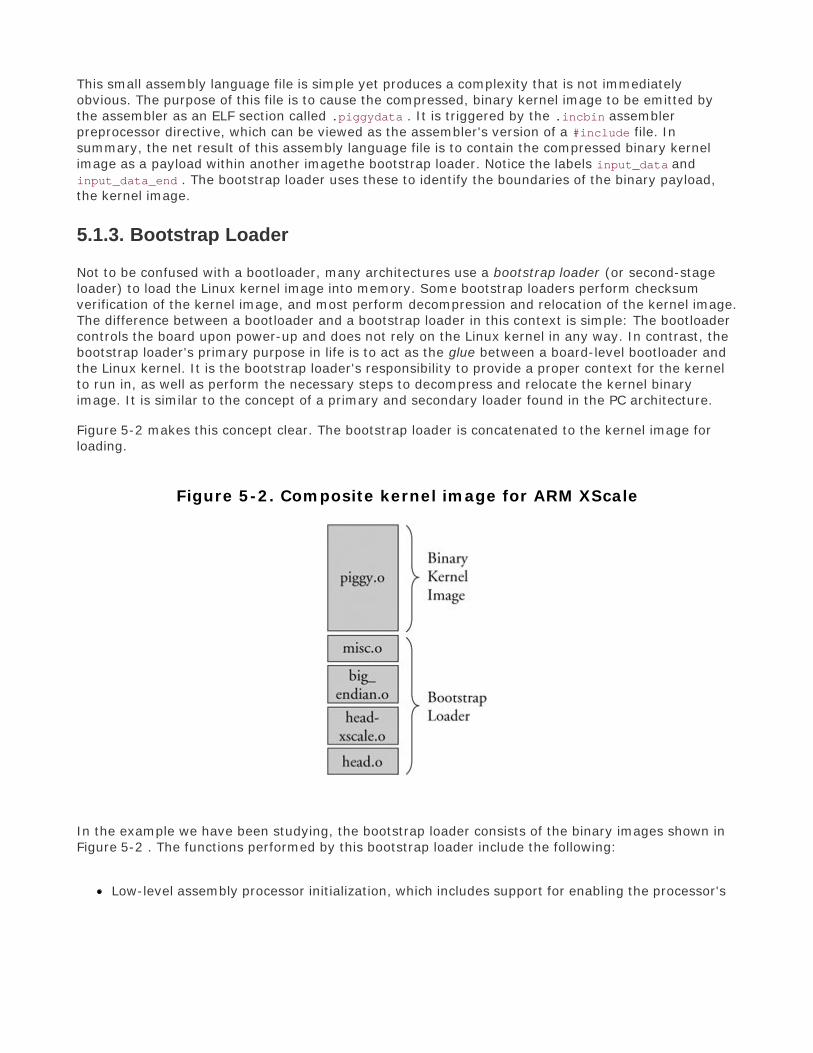
This small assembly language file is simple yet produces a complexity that is not immediatelyobvious. The purpose of this file is to cause the compressed, binary kernel image to be emitted bythe assembler as an ELF section called .piggydata . It is triggered by the .incbin assemblerpreprocessor directive, which can be viewed as the assembler's version of a #include file. Insummary, the net result of this assembly language file is to contain the compressed binary kernelimage as a payload within another imagethe bootstrap loader. Notice the labels input_data andinput_data_end . The bootstrap loader uses these to identify the boundaries of the binary payload,the kernel image.
5.1.3. Bootstrap Loader
Not to be confused with a bootloader, many architectures use a bootstrap loader (or second-stageloader) to load the Linux kernel image into memory. Some bootstrap loaders perform checksumverification of the kernel image, and most perform decompression and relocation of the kernel image.The difference between a bootloader and a bootstrap loader in this context is simple: The bootloadercontrols the board upon power-up and does not rely on the Linux kernel in any way. In contrast, thebootstrap loader's primary purpose in life is to act as the glue between a board-level bootloader andthe Linux kernel. It is the bootstrap loader's responsibility to provide a proper context for the kernelto run in, as well as perform the necessary steps to decompress and relocate the kernel binaryimage. It is similar to the concept of a primary and secondary loader found in the PC architecture.
Figure 5-2 makes this concept clear. The bootstrap loader is concatenated to the kernel image forloading.
Figure 5-2. Composite kernel image for ARM XScale
In the example we have been studying, the bootstrap loader consists of the binary images shown inFigure 5-2 . The functions performed by this bootstrap loader include the following:
Low-level assembly processor initialization, which includes support for enabling the processor's

internal instruction and data caches, disabling interrupts, and setting up a C runtimeenvironment. These include head.o and head-xscale.o .
Decompression and relocation code, embodied in misc.o .
Other processor-specific initialization, such as big-endian.o , which enables the big endianmode for this particular processor.
It is worth noting that the details we have been examining in the preceding sections are specific tothe ARM/XScale kernel implementation. Each architecture has different details, although the conceptsare similar. Using a similar analysis to that presented here, you can learn the requirements of yourown architecture.
5.1.4. Boot Messages
Perhaps you've seen a PC workstation booting a desktop Linux distribution such as Red Hat or SUSELinux. After the PC's own BIOS messages, you see a flurry of console messages being displayed byLinux as it initializes the various kernel subsystems. Significant portions of the output are commonacross disparate architectures and machines. Two of the more interesting early boot messages arethe kernel version string and the kernel command line , which is detailed shortly. Listing 5-3reproduces the kernel boot messages for the ADI Engineering Coyote Reference Platform bootingLinux on the Intel XScale IXP425 processor. The listing has been formatted with line numbers foreasy reference.
Listing 5-3. Linux Boot Messages on IPX425
[View full width]
1 Uncompressing Linux... done, booting the kernel.2 Linux version 2.6.14-clh (chris@pluto) (gcc version 3.4.3 (MontaVista 3.4.3-25.0.30.0501131 2005-07-23)) #11 Sat Mar 25 11:16:33 EST 20063 CPU: XScale-IXP42x Family [690541c1] revision 1 (ARMv5TE)4 Machine: ADI Engineering Coyote5 Memory policy: ECC disabled, Data cache writeback6 CPU0: D VIVT undefined 5 cache7 CPU0: I cache: 32768 bytes, associativity 32, 32 byte lines, 32 sets8 CPU0: D cache: 32768 bytes, associativity 32, 32 byte lines, 32 sets9 Built 1 zonelists10 Kernel command line: console=ttyS0,115200 ip=bootp root=/dev/nfs11 PID hash table entries: 512 (order: 9, 8192 bytes)12 Console: colour dummy device 80x3013 Dentry cache hash table entries: 16384 (order: 4, 65536 bytes)14 Inode-cache hash table entries: 8192 (order: 3, 32768 bytes)15 Memory: 64MB = 64MB total16 Memory: 62592KB available (1727K code, 339K data, 112K init)17 Mount-cache hash table entries: 51218 CPU: Testing write buffer coherency: ok19 softlockup thread 0 started up.20 NET: Registered protocol family 1621 PCI: IXP4xx is host22 PCI: IXP4xx Using direct access for memory space23 PCI: bus0: Fast back to back transfers enabled

24 dmabounce: registered device 0000:00:0f.0 on pci bus25 NetWinder Floating Point Emulator V0.97 (double precision)26 JFFS2 version 2.2. (NAND) (C) 2001-2003 Red Hat, Inc.27 Serial: 8250/16550 driver $Revision: 1.90 $ 2 ports, IRQ sharing disabled28 ttyS0 at MMIO 0xc8001000 (irq = 13) is a XScale29 io scheduler noop registered30 io scheduler anticipatory registered31 io scheduler deadline registered32 io scheduler cfq registered33 RAMDISK driver initialized: 16 RAM disks of 8192K size 1024 blocksize34 loop: loaded (max 8 devices)35 eepro100.c:v1.09j-t 9/29/99 Donald Becker http://www.scyld.com/network/eepro100.html36 eepro100.c: $Revision: 1.36 $ 2000/11/17 Modified by Andrey V. Savochkin <[email protected]> and others37 eth0: 0000:00:0f.0, 00:0E:0C:00:82:F8, IRQ 28.38 Board assembly 741462-016, Physical connectors present: RJ4539 Primary interface chip i82555 PHY #1.40 General self-test: passed.41 Serial sub-system self-test: passed.42 Internal registers self-test: passed.43 ROM checksum self-test: passed (0x8b51f404).44 IXP4XX-Flash.0: Found 1 x16 devices at 0x0 in 16-bit bank45 Intel/Sharp Extended Query Table at 0x003146 Using buffer write method47 cfi_cmdset_0001: Erase suspend on write enabled48 Searching for RedBoot partition table in IXP4XX-Flash.0 at offset 0xfe000049 5 RedBoot partitions found on MTD device IXP4XX-Flash.050 Creating 5 MTD partitions on "IXP4XX-Flash.0":51 0x00000000-0x00060000 : "RedBoot"52 0x00100000-0x00260000 : "MyKernel"53 0x00300000-0x00900000 : "RootFS"54 0x00fc0000-0x00fc1000 : "RedBoot config"55 mtd: partition "RedBoot config" doesn't end on an erase block -- force read-only0x00fe0000-0x01000000 : "FIS directory"56 NET: Registered protocol family 257 IP route cache hash table entries: 1024 (order: 0, 4096 bytes)58 TCP established hash table entries: 4096 (order: 2, 16384 bytes)59 TCP bind hash table entries: 4096 (order: 2, 16384 bytes)60 TCP: Hash tables configured (established 4096 bind 4096)61 TCP reno registered62 TCP bic registered63 NET: Registered protocol family 164 Sending BOOTP requests . OK65 IP-Config: Got BOOTP answer from 192.168.1.10, my address is 192.168.1.14166 IP-Config: Complete:67 device=eth0, addr=192.168.1.141, mask=255.255.255.0, gw=255.255.255.255,68 host=192.168.1.141, domain=, nis-domain=(none),69 bootserver=192.168.1.10, rootserver=192.168.1.10, rootpath=/home/chris/sandbox/coyote-target70 Looking up port of RPC 100003/2 on 192.168.1.1071 Looking up port of RPC 100005/1 on 192.168.1.10

72 VFS: Mounted root (nfs filesystem).73 Freeing init memory: 112K74 Mounting proc75 Starting system loggers76 Configuring lo77 Starting inetd78 / #
The kernel produces much useful information during startup, as shown in Listing 5-3 . We study thisoutput in some detail in the next few sections. Line 1 is produced by the bootstrap loader wepresented earlier in this chapter. This message was produced by the decompression loader found in…/arch/arm/boot/compressed/misc.c .
Line 2 of Listing 5-3 is the kernel version string. It is the first line of output from the kernel itself. Oneof the first lines of C code executed by the kernel (in .../init/main.c ) upon entering start_kernel()is as follows:
printk(linux_banner);
This line produces the output just describedthe kernel version string, Line 2 of Listing 5-3 . Thisversion string contains a number of pertinent data points related to the kernel image:
Kernel version: Linux version 2.6.10-clh
Username/machine name where kernel was compiled
Toolchain info: gcc version 3.4.3, supplied by MontaVista Software
Build number
Date and time compiled
This is useful information both during development and later in production. All but one of the entriesare self-explanatory. The build number is simply a tool that the developers added to the versionstring to indicate that something more substantial than the date and time changed from one build tothe next. It is a way for developers to keep track of the build in a generic and automatic fashion. Youwill notice in this example that this was the eleventh build in this series, as indicated by the #11 online 2 of Listing 5-3 . The version string is stored in a hidden file in the top-level Linux directory and iscalled .version . It is automatically incremented by a build script found in .../scripts/mkversion andby the top-level makefile. In short, it is a version string that is automatically incremented wheneveranything substantial in the kernel is rebuilt.

5.2. Initialization Flow of Control
Now that we have an understanding of the structure and components of the composite kernel image,let's examine the flow of control from the bootloader to the kernel in a complete boot cycle. As wediscussed in Chapter 2, "Your First Embedded Experience," the bootloader is the low-level componentresident in system nonvolatile memory (Flash or ROM) that takes control immediately after the powerhas been applied. It is typically a small, simple set of routines designed primarily to do low-levelinitialization, boot image loading, and system diagnostics. It might contain memory dump and fillroutines for examining and modifying the contents of memory. It might also contain low-level boardself-test routines, including memory and I/O tests. Finally, a bootloader contains logic for loading andpassing control to another program, usually an operating system such as Linux.
The ARM XScale platform used as a basis for the examples in this chapter contains the Redbootbootloader. When power is first applied, this bootloader is invoked and proceeds to load the operatingsystem (OS). When the bootloader locates and loads the OS image (which could be resident locally inFlash, on a hard drive, or via a local area network or other device), control is passed to that image.
On this particular XScale platform, the bootloader passes control to our head.o module at the labelStart in the bootstrap loader. This is illustrated in Figure 5-3.
Figure 5-3. ARM boot control flow
As detailed earlier, the bootstrap loader prepended to the kernel image has a single primaryresponsibility: to create the proper environment to decompress and relocate the kernel, and passcontrol to it. Control is passed from the bootstrap loader directly to the kernel proper, to a modulecalled head.o for most architectures. It is an unfortunate historical artifact that both the bootstraploader and the kernel proper contain a module called head.o because it is a source of confusion to thenew embedded Linux developer. The head.o module in the bootstrap loader might be moreappropriately called kernel_bootstrap_loader_head.o, although I doubt that the kernel developers

would accept this patch. In fact, a recent Linux 2.6 source tree contains no fewer than 37 source filesnamed head.S. This is another reason why you need to know your way around the kernel source tree.
Refer back to Figure 5-3 for a graphical view of the flow of control. When the bootstraploader hascompleted its job, control is passed to the kernel proper's head.o, and from there to start_kernel()in main.c.
5.2.1. Kernel Entry Point: head.o
The intention of the kernel developers was to keep the architecture-specific head.o module verygeneric, without any specific machine[4] dependencies. This module, derived from the assemblylanguage file head.S, is located at .../arch/<ARCH>/kernel/head.S, where <ARCH> is replaced by thegiven architecture. The examples in this chapter are based on the ARM/XScale, as you have seen,with <ARCH>=arm.
[4] The term machine as used here refers to a specific hardware reference platform.
The head.o module performs architecture- and often CPU-specific initialization in preparation for themain body of the kernel. CPU-specific tasks are kept as generic as possible across processor families.Machine-specific initialization is performed elsewhere, as you will discover shortly. Among other low-level tasks, head.o performs the following tasks:
Checks for valid processor and architecture
Creates initial page table entries
Enables the processor's memory management unit (MMU)
Establishes limited error detection and reporting
Jumps to the start of the kernel proper, main.c
These functions contain some hidden complexities. Many novice embedded developers have tried tosingle-step through parts of this code, only to find that the debugger becomes hopelessly lost.Although a discussion of the complexities of assembly language and the hardware details of virtualmemory is beyond the scope of this book, a few things are worth noting about this complicatedmodule.
When control is first passed to the kernel's head.o from the bootstrap loader, the processor isoperating in what we used to call real mode in x86 terminology. In effect, the logical addresscontained in the processor's program counter[5] (or any other register, for that matter) is the actualphysical address driven onto the processor's electrical memory address pins. Soon after theprocessor's registers and kernel data structures are initialized to enable memory translation, theprocessor's memory management unit (MMU) is turned on. Suddenly, the address space as seen bythe processor is yanked from beneath it and replaced by an arbitrary virtual addressing schemedetermined by the kernel developers. This creates a complexity that can really be understood only bya detailed analysis of both the assembly language constructs and logical flow, as well as a detailedknowledge of the CPU and its hardware address translation mechanism. In short, physical addressesare replaced by logical addresses the moment the MMU is enabled. That's why a debugger can'tsingle-step through this portion of code as with ordinary code.

[5] Often called Instruction Pointer, the register which holds the address of the next machine instruction in memory.
The second point worth noting is the limited available mapping at this early stage of the kernel bootprocess. Many developers have stumbled into this limitation while trying to modify head.o for theirparticular platform.[6] One such scenario might go like this. Let's say you have a hardware devicethat needs a firmware load very early in the boot cycle. One possible solution is to compile thenecessary firmware statically into the kernel image and then reference it via a pointer to download itto your device. However, because of the limited memory mapping done at this point, it is quitepossible that your firmware image will exist beyond the range that has been mapped at this earlystage in the boot cycle. When your code executes, it generates a page fault because you haveattempted to access a memory region for which no valid mapping has been created inside theprocessor. Worse yet, a page fault handler has not yet been installed at this early stage, so all youget is an unexplained system crash. At this early stage in the boot cycle, you are pretty muchguaranteed not to have any error messages to help you figure out what's wrong.
[6] Modifying head.S for your custom platform is highly discouraged. There is almost always a better way. See Chapter 16,
"Porting Linux," for additional information.
You are wise to consider delaying any custom hardware initialization until after the kernel has booted,if at all possible. In this manner, you can rely on the well-known device driver model for access tocustom hardware instead of trying to customize the much more complicated assembly languagestartup code. Numerous undocumented techniques are used at this level. One common example ofthis is to work around hardware errata that may or may not be documented. A much higher price willbe paid in development time, cost, and complexity if you must make changes to the early startupassembly language code. Hardware and software engineers should discuss these facts during earlystages of hardware development, when often a minor hardware change can lead to significantsavings in software development time.
It is important to recognize the constraints placed upon the developer in a virtual memoryenvironment. Many experienced embedded developers have little or no experience in thisenvironment, and the scenario presented earlier is but one small example of the pitfalls that awaitthe developer new to virtual memory architectures. Nearly all modern 32-bit and largermicroprocessors have memory-management hardware used to implement virtual memoryarchitectures. One of the most significant advantages of virtual memory machines is that they helpseparate teams of developers write large complex applications, while protecting other softwaremodules, and the kernel itself, from programming errors.
5.2.2. Kernel Startup: main.c
The final task performed by the kernel's own head.o module is to pass control to the primary kernelstartup file written in C. We spend a good portion of the rest of this chapter on this important file.
For each architecture, there is a different syntax and methodology, but every architecture's head.omodule has a similar construct for passing control to the kernel proper. For the ARM architecture itlooks as simple as this:
b start_kernel
For PowerPC, it looks similar to this:

lis r4,start_kernel@h ori r4,r4,start_kernel@l lis r3,MSR_KERNEL@h ori r3,r3,MSR_KERNEL@l mtspr SRR0,r4 mtspr SRR1,r3 rfi
Without going into details of the specific assembly language syntax, both of these examples result inthe same thing. Control is passed from the kernel's first object module (head.o) to the C languageroutine start_kernel() located in .../init/main.c. Here the kernel begins to develop a life of itsown.
The file main.c should be studied carefully by anyone seeking a deeper understanding of the Linuxkernel, what components make it up, and how they are initialized and/or instantiated. main.c does allthe startup work for the Linux kernel, from initializing the first kernel thread all the way to mountinga root file system and executing the very first user space Linux application program.
The function start_kernel() is by far the largest function in main.c. Most of the Linux kernelinitialization takes place in this routine. Our purpose here is to highlight those particular elementsthat will prove useful in the context of embedded systems development. It is worth repeating:Studying main.c is a great way to spend your time if you want to develop a better understanding ofthe Linux kernel as a system.
5.2.3. Architecture Setup
Among the first few things that happen in .../init/main.c in the start_kernel() function is the callto setup_arch(). This function takes a single parameter, a pointer to the kernel command lineintroduced earlier and detailed in the next section.
setup_arch(&command_line);
This statement calls an architecture-specific setup routine responsible for performing initializationtasks common across each major architecture. Among other functions, setup_arch() calls functionsthat identify the specific CPU and provides a mechanism for calling high-level CPU-specificinitialization routines. One such function, called directly by setup_arch(), is setup_processor(), foundin .../arch/arm/kernel/setup.c. This function verifies the CPU ID and revision, calls CPU-specificinitialization functions, and displays several lines of information on the console during boot.
An example of this output can be found in Listing 5-3, lines 3 through 8. Here you can see the CPUtype, ID string, and revision read directly from the processor core. This is followed by details of theprocessor cache type and size. In this example, the IXP425 has a 32KB I (instruction) cache and32KB D (data) cache, along with other implementation details of the internal processor cache.
One of the final actions of the architecture setup routines is to perform any machine-dependentinitialization. The exact mechanism for this varies across different architectures. For ARM, you willfind machine-specific initialization in the .../arch/arm/mach-* series of directories, depending on yourmachine type. MIPS architecture also contains directories specific to supported reference platforms.For PowerPC, there is a machine-dependent structure that contains pointers to many common setup

functions. We examine this in more detail in Chapter 16, "Porting Linux."

5.3. Kernel Command Line Processing
Following the architecture setup, main.c performs generic early kernel initialization and then displaysthe kernel command line. Line 10 of Listing 5-3 is reproduced here for convenience.
Kernel command line: console=ttyS0,115200 ip=bootp root=/dev/nfs
In this simple example, the kernel being booted is instructed to open a console device on serial portdevice ttyS0 (usually the first serial port) at a baud rate of 115Kbps. It is being instructed to obtainits initial IP address information from a BOOTP server and to mount a root file system via the NFSprotocol. (We cover BOOTP later in Chapter 12 , "Embedded Development Environment," and NFS inChapters 9 , "File Systems," and 12 . For now, we limit the discussion to the kernel command linemechanism.)
Linux is typically launched by a bootloader (or bootstrap loader) with a series of parameters thathave come to be called the kernel command line . Although we don't actually invoke the kernel usinga command prompt from a shell, many bootloaders can pass parameters to the kernel in a fashionthat resembles this well-known model. On some platforms whose bootloaders are not Linux aware,the kernel command line can be defined at compile time and becomes hard coded as part of thekernel binary image. On other platforms (such as a desktop PC running Red Hat Linux), thecommand line can be modified by the user without having to recompile the kernel. The bootstraploader (Grub or Lilo in the desktop PC case) builds the kernel command line from a configuration fileand passes it to the kernel during the boot process. These command line parameters are a bootmechanism to set initial configuration necessary for proper boot on a given machine.
Numerous command line parameters are defined throughout the kernel. The .../Documentationsubdirectory in the kernel source contains a file called kernel-parameters.txt containing a list ofkernel command line parameters in dictionary order. Remember the previous warning about kerneldocumentation: The kernel changes far faster than the documentation. Use this file as a guide, butnot a definitive reference. More than 400 distinct kernel command line parameters are documented inthis file, and it cannot be considered a comprehensive list. For that, you must refer directly to thesource code.
The basic syntax for kernel command line parameters is fairly simple and mostly evident from theexample in line 10 of Listing 5-3 . Kernel command line parameters can be either a single text word,a key=value pair, or a key= value1, value2, …. key and multivalue format. It is up to the consumerof this information to process the data as delivered. The command line is available globally and isprocessed by many modules as needed. As noted earlier, setup_arch() in main.c is called with thekernel command line as its only argument. This is to pass architecture-specific parameters andconfiguration directives to the relevant portions of architecture- and machine-specific code.
Device driver writers and kernel developers can add additional kernel command-line parameters fortheir own specific needs. Let's take a look at the mechanism. Unfortunately, some complications areinvolved in using and processing kernel command line parameters. The first of these is that theoriginal mechanism is being deprecated in favor of a much more robust implementation. The second

complication is that we need to comprehend the complexities of a linker script file to fully understandthe mechanism.[7]
[7] It's not necessarily all that complex, but most of us never need to understand a linker script file. The embedded engineer does.
It is well documented in the GNU LD manual referenced at the end of this chapter.
5.3.1. The __setup Macro
As an example of the use of kernel command line parameters, consider the specification of theconsole device. We want this device to be initialized early in the boot cycle so that we have adestination for console messages during boot. This initialization takes place in a kernel object calledprintk.o . The C source file for this module is found in .../kernel/printk.c . The consoleinitialization routine is called console_setup() and takes the kernel command line parameter string asits only argument.
The challenge is to communicate the console parameters specified on the kernel command line to thesetup and device driver routines that require this data in a modular and general fashion. Furthercomplicating the issue is that typically the command line parameters are required early, before (or intime for) those modules that need them. The startup code in main.c , where the main processing ofthe kernel command line takes place, cannot possibly know the destination functions for each ofhundreds of kernel command line parameters without being hopelessly polluted with knowledge fromevery consumer of these parameters. What is needed is a flexible and generic way to pass thesekernel command line parameters to their consumers.
In Linux 2.4 and earlier kernels, developers used a simple macro to generate a not-so-simplesequence of code. Although it is being deprecated, the __setup macro is still in widespread usethroughout the kernel. We next use the kernel command line from Listing 5-3 to demonstrate howthe __setup macro works.
From the previous kernel command line (line 10 of Listing 5-3 ), this is the first complete commandline parameter passed to the kernel:
console=ttyS0,115200
For the purposes of this example, the actual meaning of the parameters is irrelevant. Our goal here isto illustrate the mechanism, so don't be concerned if you don't understand the argument or itsvalues.
Listing 5-4 is a snippet of code from .../kernel/printk.c . The body of the function has beenstripped because it is not relevant to the discussion. The most relevant part of Listing 5-4 is the lastline, the invocation of the __setup macro. This macro expects two arguments; in this case, it ispassed a string literal and a function pointer. It is no coincidence that the string literal passed to the__setup macro is the same as the first eight characters of the kernel command line related to theconsole: console= .
Listing 5-4. Console Setup Code Snippet
/* * Setup a list of consoles. Called from init/main.c */

static int __init console_setup(char *str){ char name[sizeof(console_cmdline[0].name)]; char*s, *options; int idx;
/* * Decode str into name, index, options. */
return 1;}
__setup("console=", console_setup);
You can think of this macro as a registration function for the kernel command-line consoleparameter. In effect, it says: When the console= string is encountered on the kernel command line,invoke the function represented by the second __setup macro argumentin this case, theconsole_setup() function. But how is this information communicated to the early setup code, outsidethis module, which has no knowledge of the console functions? The mechanism is both clever andsomewhat complicated, and relies on lists built by the linker.
The details are hidden in a set of macros designed to conceal the syntactical tedium of adding sectionattributes (and other attributes) to a portion of object code. The objective is to build a static list ofstring literals associated with function pointers. This list is emitted by the compiler in a separatelynamed ELF section in the final vmlinux ELF image. It is important to understand this technique; it isused in several places within the kernel for special-purpose processing.
Let's now examine how this is done for the __setup macro case. Listing 5-5 is a portion of code fromthe header file .../include/linux/init.h defining the __setup family of macros.
Listing 5-5. Family of __setup Macro Definitions from init.h
...#define __setup_param(str, unique_id, fn, early) \ static char __setup_str_##unique_id[] __initdata = str; \ static struct obs_kernel_param __setup_##unique_id \ __attribute_used__ \ __attribute__((__section__(".init.setup"))) \ __attribute__((aligned((sizeof(long))))) \ = { __setup_str_##unique_id, fn, early }
#define __setup_null_param(str, unique_id) \ __setup_param(str, unique_id, NULL, 0)
#define __setup(str, fn\ __setup_param(str, fn, fn, 0)...

Listing 5-5 is the author's definition of syntactical tedium! Recall from Listing 5-4 that our invocationof the original __setup macro looked like this:
__setup("console=", console_setup);
With some slight simplification, here is what the compiler's preprocessor produces after macroexpansion:
static char __setup_str_console_setup[] __initdata = "console="; static struct obs_kernel_param __setup_console_setup \ __attribute__((__section__(".init.setup")))= {__setup_str_console_setup, console_setup, 0};
To make this more readable, we have split the second and third lines, as indicated by the UNIX line-continuation character \.
We have intentionally left out two compiler attributes whose description does not add any insight tothis discussion. Briefly, the __attribute_used__ (itself a macro hiding further syntactical tedium) tellsthe compiler to emit the function or variable, even if the optimizer determines that it is unused.[8]
The __attribute__ (aligned) tells the compiler to align the structures on a specific boundary, in thiscase sizeof(long) .
[8] Normally, the compiler will complain if a variable is defined static and never referenced in the compilation unit. Because these
variables are not explicitly referenced, the warning would be emitted without this directive.
What we have left after simplification is the heart of the mechanism. First, the compiler generates anarray of characters called __setup_str_console_ setup[] initialized to contain the string console= .Next, the compiler generates a structure that contains three members: a pointer to the kernelcommand line string (the array just declared), the pointer to the setup function itself, and a simpleflag. The key to the magic here is the section attribute attached to the structure. This attributeinstructs the compiler to emit this structure into a special section within the ELF object module, called.init.setup . During the link stage, all the structures defined using the __setup macro are collectedand placed into this .init .setup section, in effect creating an array of these structures. Listing 5-6 ,a snippet from .../init/main.c , shows how this data is accessed and used.
Listing 5-6. Kernel Command Line Processing
1 extern struct obs_kernel_param __setup_start[], __setup_end[];23 static int __init obsolete_checksetup(char *line)4 {5 struct obs_kernel_param *p;67 p = __setup_start;8 do {9 int n = strlen(p->str);10 if (!strncmp(line, p->str, n)) {11 if (p->early) {12 /* Already done in parse_early_param? (Needs13 * exact match on param part) */

14 if (line[n] == '\0' || line[n] == '=')15 return 1;16 } else if (!p->setup_func) {17 printk(KERN_WARNING "Parameter %s is obsolete,"18 " ignored\n", p->str);19 return 1;20 } else if (p->setup_func(line + n))21 return 1;22 }23 p++;24 } while (p < __setup_end);25 return 0;26 }
Examination of this code should be fairly straightforward, with a couple of explanations. The functionis called with a single command line argument, parsed elsewhere within main.c . In the examplewe've been discussing, line would point to the string console=ttyS0 ,115200 , which is onecomponent from the kernel command line. The two external structure pointers __setup_start and__setup_end are defined in a linker script file, not in a C source or header file. These labels mark thestart and end of the array of obs_kernel_param structures that were placed in the .init.setup sectionof the object file.
The code in Listing 5-6 scans all these structures via the pointer p to find a match for this particularkernel command line parameter. In this case, the code is searching for the string console= and findsa match. From the relevant structure, the function pointer element returns a pointer to theconsole_setup() function, which is called with the balance of the parameter (the string ttyS0 ,115200) as its only argument. This process is repeated for every element in the kernel command line untilthe kernel command line has been completely exhausted.
The technique just described, collecting objects into lists in uniquely named ELF sections, is used inmany places in the kernel. Another example of this technique is the use of the __init family ofmacros to place one-time initialization routines into a common section in the object file. Its cousin__initdata , used to mark one-time-use data items, is used by the __setup macro. Functions anddata marked as initialization using these macros are collected into a specially named ELF section.Later, after these one-time initialization functions and data objects have been used, the kernel freesthe memory occupied by these items. You might have seen the familiar kernel message near the finalpart of the boot process saying, "Freeing init memory: 296K." Your mileage may vary, but a third ofa megabyte is well worth the effort of using the __init family of macros. This is exactly the purposeof the __initdata macro in the earlier declaration of __setup_str_console_setup[] .
You might have been wondering about the use of symbol names preceded with obsolete_ . This isbecause the kernel developers are replacing the kernel command line processing mechanism with amore generic mechanism for registering both boot time and loadable module parameters. At thepresent time, hundreds of parameters are declared with the __setup macro. However, newdevelopment is expected to use the family of functions defined by the kernel header file.../include/linux/moduleparam.h , most notably, the family of module_param* macros. These areexplained in more detail in Chapter 8 , "Device Driver Basics," when we introduce device drivers.
The new mechanism maintains backward compatibility by including an unknown function pointerargument in the parsing routine. Thus, parameters that are unknown to the module_param*infrastructure are considered unknown, and the processing falls back to the old mechanism under

control of the developer. This is easily understood by examining the well-written code in.../kernel/params.c and the parse_args() calls in .../init/main.c .
The last point worth mentioning is the purpose of the flag member of the obs_kernel_param structurecreated by the __setup macro. Examination of the code in Listing 5-6 should make it clear. The flag inthe structure, called early , is used to indicate whether this particular command line parameter wasalready consumed earlier in the boot process. Some command line parameters are intended forconsumption very early in the boot process, and this flag provides a mechanism for an early parsingalgorithm. You will find a function in main.c called do_early_param() that traverses the linker-generated array of __setup- generated structures and processes each one marked for earlyconsumption. This gives the developer some control over when in the boot process this processing isdone.

5.4. Subsystem Initialization
Many kernel subsystems are initialized by the code found in main.c. Some are initialized explicitly, aswith the calls to init_timers() and console_init(), which need to be called very early. Others areinitialized using a technique very similar to that described earlier for the __setup macro. In short, thelinker builds lists of function pointers to various initialization routines, and a simple loop is used toexecute each in turn. Listing 5-7 shows how this works.
Listing 5-7. Example Initialization Routine
static int __init customize_machine(void){ /* customizes platform devices, or adds new ones */ if (init_machine) init_machine(); return 0;}arch_initcall(customize_machine);
This code snippet comes from .../arch/arm/kernel/setup.c. It is a simple routine designed toprovide a customization hook for a particular board.
5.4.1. The *__initcall Macros
Notice two important things about the initialization routine in Listing 5-7. First, it is defined with the__init macro. As we saw earlier, this macro applies the section attribute to declare that this functiongets placed into a section called .init.text in the vmlinux ELF file. Recall that the purpose of placingthis function into a special section of the object file is so the memory space that it occupies can bereclaimed when it is no longer needed.
The second thing to notice is the macro immediately following the definition of the function:arch_initcall(customize_machine). This macro is part of a family of macros defined in.../include/linux/init.h. These macros are reproduced here as Listing 5-8.
Listing 5-8. initcall Family of Macros

#define __define_initcall(level,fn) \ static initcall_t __initcall_##fn __attribute_used__ \ __attribute__((__section__(".initcall" level ".init"))) = fn
#define core_initcall(fn) __define_initcall("1",fn)#define postcore_initcall(fn) __define_initcall("2",fn)#define arch_initcall(fn) __define_initcall("3",fn)#define subsys_initcall(fn) __define_initcall("4",fn)#define fs_initcall(fn) __define_initcall("5",fn)#define device_initcall(fn) __define_initcall("6",fn)#define late_initcall(fn) __define_initcall("7",fn)
In a similar fashion to the __setup macro previously detailed, these macros declare a data item basedon the name of the function, and use the section attribute to place this data item into a uniquelynamed section of the vmlinux ELF file. The benefit of this approach is that main.c can call an arbitraryinitialization function for a subsystem that it has no knowledge of. The only other option, asmentioned earlier, is to pollute main.c with knowledge of every subsystem in the kernel.
As you can see from Listing 5-8, the name of the section is .initcallN.init, where N is the leveldefined between 1 and 7. The data item is assigned the address of the function being named in themacro. In the example defined by Listings 5-7 and 5-8, the data item would be as follows (simplifiedby omitting the section attribute):
static initcall_t __initcall_customize_machine = customize_machine;
This data item is placed in the kernel's object file in a section called .initcall1.init.
The level (N) is used to provide an ordering of initialization calls. Functions declared using thecore_initcall() macro are called before all others. Functions declared using thepostcore_initcall() macros are called next, and so on, while those declared with late_initcall()are the last initialization functions to be called.
In a fashion similar to the __setup macro, you can think of this family of *_initcall macros asregistration functions for kernel subsystem initialization routines that need to be run once at kernelstartup and then never used again. These macros provide a mechanism for causing the initializationroutine to be executed during system startup, and a mechanism to discard the code and reclaim thememory after the routine has been executed. The developer is also provided up to seven levels ofwhen to perform the initialization routines. Therefore, if you have a subsystem that relies on anotherbeing available, you can enforce this ordering using these levels. If you grep the kernel for the string[a-z]*_initcall, you will see that this family of macros is used extensively.
One final note about the *_initcall family of macros: The use of multiple levels was introducedduring the development of the 2.6 kernel series. Earlier kernel versions used the __initcall() macrofor this purpose. This macro is still in widespread use, especially in device drivers. To maintainbackward compatibility, this macro has been defined to device_initcall(), which has been definedas a level 6 initcall.

5.5. The init Thread
The code found in .../init/main.c is responsible for bringing the kernel to life. After start_kernel()performs some basic kernel initialization, calling early initialization functions explicitly by name, thevery first kernel thread is spawned. This thread eventually becomes the kernel thread called init(),with a process id (PID) of 1. As you will learn, init() becomes the parent of all Linux processes inuser space. At this point in the boot sequence, two distinct threads are running: that represented bystart_kernel() and now init(). The former goes on to become the idle process, having completedits work. The latter becomes the init process. This can be seen in Listing 5-9.
Listing 5-9. Creation of Kernel init THRead
static void noinline rest_init(void) __releases(kernel_lock){ kernel_thread(init, NULL, CLONE_FS | CLONE_SIGHAND); numa_default_policy(); unlock_kernel(); preempt_enable_no_resched();
/* * The boot idle thread must execute schedule() * at least one to get things moving: */ schedule();
cpu_idle();}
The start_kernel() function calls rest_init(), reproduced in Listing 5-9. The kernel's init process isspawned by the call to kernel_thread().init goes on to complete the rest of the systeminitialization, while the thread of execution started by start_kernel() loops forever in the call tocpu_idle().
The reason for this structure is interesting. You might have noticed that start_kernel(), a relativelylarge function, was marked with the __init macro. This means that the memory it occupies will bereclaimed during the final stages of kernel initialization. It is necessary to exit this function and theaddress space that it occupies before reclaiming its memory. The answer to this was forstart_kernel() to call rest_init(), shown in Listing 5-9, a much smaller piece of memory thatbecomes the idle process.
5.5.1. Initialization via initcalls

When init() is spawned, it eventually calls do_initcalls(), which is the function responsible forcalling all the initialization functions registered with the *_initcall family of macros. The code isreproduced in Listing 5-10 in simplified form.
Listing 5-10. Initialization via initcalls
static void __init do_initcalls(void){ initcall_t *call;
for( call = &__initcall_start; call < &__initcall_end; call++) {
if (initcall_debug) { printk(KERN_DEBUG "Calling initcall 0x%p", *call); print_symbol(":%s()", (unsigned long) *call); printk("\n"); }
(*call)();
}
This code is self-explanatory, except for the two labels marking the loop boundaries:__initcall_start and __initcall_end. These labels are not found in any C source or header file.They are defined in the linker script file used during the link stage of vmlinux. These labels mark thebeginning and end of the list of initialization functions populated using the *_initcall family ofmacros. You can see each of the labels by looking at the System.map file in the top-level kerneldirectory. They all begin with the string __initcall, as described in Listing 5-8.
In case you were wondering about the debug print statements in do_initcalls(), you can watchthese calls being executed during bootup by setting the kernel command line parameterinitcall_debug. This command line parameter enables the printing of the debug information shownin Listing 5-10. Simply start your kernel with the kernel command line parameter initcall_debug toenable this diagnostic output.[9]
[9] You might have to lower the default loglevel on your system to see these debug messages. This is described in many
references about Linux system administration. In any case, you should see them in the kernel log file.
Here is an example of what you will see when you enable these debug statements:
...Calling initcall 0xc00168f4: tty_class_init+0x0/0x3c()Calling initcall 0xc000c32c: customize_machine+0x0/0x2c()Calling initcall 0xc000c4f0: topology_init+0x0/0x24()Calling initcall 0xc000e8f4: coyote_pci_init+0x0/0x20()PCI: IXP4xx is hostPCI: IXP4xx Using direct access for memory space

...
Notice the call to customize_machine(), the example of Listing 5-7. The debug output includes thevirtual kernel address of the function (0xc000c32c, in this case) and the size of the function (0x2chere.) This is a useful way to see the details of kernel initialization, especially the order in whichvarious subsystems and modules get called. Even on a modestly configured embedded system,dozens of these initialization functions are invoked in this manner. In this example taken from anARM XScale embedded target, there are 92 such calls to various kernel-initialization routines.
5.5.2. Final Boot Steps
Having spawned the init() thread and all the various initialization calls have completed, the kernelperforms its final steps in the boot sequence. These include freeing the memory used by theinitialization functions and data, opening a system console device, and starting the first userspaceprocess. Listing 5-11 reproduces the last steps in the kernel's init() from main.c.
Listing 5-11. Final Kernel Boot Steps from main.c
if (execute_command) { run_init_process(execute_command); printk(KERN_WARNING "Failed to execute %s. Attempting " "defaults...\n", execute_command);}
run_init_process("/sbin/init");run_init_process("/etc/init");run_init_process("/bin/init");run_init_process("/bin/sh");
panic("No init found. Try passing init= option to kernel.");
Notice that if the code proceeds to the end of the init() function, a kernel panic results. If you'vespent any time experimenting with embedded systems or custom root file systems, you'veundoubtedly encountered this very common error message as the last line of output on your console.It is one of the most frequently asked questions (FAQs) on a variety of public forums related to Linuxand embedded systems.
One way or another, one of these run_init_process() commands must proceed without error. Therun_init_process() function does not return on successful invocation. It overwrites the callingprocess with the new one, effectively replacing the current process with the new one. It uses thefamiliar execve() system call for this functionality. The most common system configurations spawn/sbin/init as the userland[10] initialization process. We study this functionality in depth in the nextchapter.
[10] Userland is an often-used term for any program, library, script, or anything else in user space.

One option available to the embedded system developer is to use a custom userland initializationprogram. That is the purpose of the conditional statement in the previous code snippet. Ifexecute_command is non-null, it points to a string containing a custom user-supplied command to beexecuted in user space. The developer specifies this command on the kernel command line, and it isset via the __setup macro we examined earlier in this chapter. An example kernel command lineincorporating several concepts discussed in this chapter might look like this:
initcall_debug init=/sbin/myinit console=ttyS1,115200 root=/dev/hda1
This kernel command line instructs the kernel to display all the initialization routines as encountered,configures the initial console device as /dev/ttyS1 at 115 kbps, and executes a custom user spaceinitialization process called myinit, located in the /sbin directory on the root file system. It directsthe kernel to mount its root file system from the device /dev/hda1, which is the first IDE hard drive.Note that, in general, the order of parameters given on the kernel command line is irrelevant. Thenext chapter covers the details of user space system initialization.

5.6. Chapter Summary
The Linux kernel project is large and complex. Understanding the structure and composition ofthe final image is key to learning how to customize your own embedded project.
Many architectures concatenate an architecture-specific bootstrap loader onto the kernel binaryimage to set up the proper execution environment required by the Linux kernel. We presentedthe bootstrap loader build steps to differentiate this functionality from the kernel proper.
Understanding the initialization flow of control will help deepen your knowledge of the Linuxkernel and provide insight into how to customize for your particular set of requirements.
We found the kernel entry point in head.o and followed the flow of control into the first kernel Cfile, main.c. We looked at a booting system and the messages it produced, along with anoverview of many of the important initialization concepts.
The kernel command line processing and the mechanisms used to declare and process kernelcommand line parameters was presented. This included a detailed look at some advancedcoding techniques for calling arbitrary unknown setup routines using linker-produced tables.
The final kernel boots steps produce the first userspace processes. Understanding thismechanism and its options will enable you to customize and troubleshoot embedded Linuxstartup issues.
5.6.1. Suggestions for Additional Reading
GNU Compiler Collection documentation:
http://gcc.gnu.org/onlinedocs/gcc[11]
[11] Especially the sections on function attributes, type attributes, and variable attributes.
Using LD, the GNU linker
http://www.gnu.org/software/binutils/manual/ld-2.9.1/ld.html
Kernel documentation:
.../Documentation/kernel-parameters.txt

Chapter 6. System InitializationIn this chapter
Root File System page 130
Kernel's Last Boot Steps page 136
The Init Process page 139
Initial RAM Disk page 145
Using initramfs page 152
Shutdown page 153
Chapter Summary page 154
In Chapter 2, "Your First Embedded Experience," we pointed out that the Linux kernel itself is but asmall part of any embedded Linux system. After the kernel has initialized itself, it must mount a rootfile system and execute a set of developer-defined initialization routines. In this chapter, we examinethe details of post-kernel system initialization.
We begin by looking at the root file system and its layout. Next we develop and study a minimalsystem configuration. Later in this chapter, we add functionality to the minimal system configurationto produce useful example embedded system configurations. We complete the coverage of systeminitialization by introducing the initial ramdisk, or initrd, and its operation and use. The chapterconcludes with a brief look at Linux shutdown logic.

6.1. Root File System
In Chapter 5, "Kernel Initialization," we examined the Linux kernel's behavior during the initializationprocess. We made several references to mounting a root file system. Linux, like many otheradvanced operating systems, requires a root file system to realize the benefits of its services.Although it is certainly possible to use Linux in an environment without a file system, it makes littlesense because most of the features and value of Linux would be lost. It would be similar to puttingyour entire system application into an overbloated device driver or kernel thread.
The root file system refers to the file system mounted at the base of the file system hierarchy,designated simply as /. As you will discover in Chapter 9, "File Systems," even a small embeddedLinux system typically mounts several file systems on different locations in the file system hierarchy.The proc file system, introduced in Chapter 9, is an example. It is a special-purpose file systemmounted at /proc under the root file system. The root file system is simply the first file systemmounted at the base of the file system hierarchy.
As you will shortly see, the root file system has special requirements for a Linux system. Linuxexpects the root file system to contain programs and utilities to boot a system, initialize services suchas networking and a system console, load device drivers, and mount additional file systems.
6.1.1. FHS: File System Hierarchy Standard
Several kernel developers authored a standard governing the organization and layout of a UNIX filesystem. The File System Hierarchy Standard (FHS) establishes a minimum baseline of compatibilitybetween Linux distributions and application programs. You'll find a reference to this standard inSection 6.7.1 "Suggestions for Additional Reading" at the end of this chapter. You are encouraged toreview the FHS standard for a better background on the layout and rationale of UNIX file systemorganization.
Many Linux distributions have directory layouts closely matching that described in the FHS standard.The standard exists to provide one element of a common base between different UNIX and Linuxdistributions. The FHS standard allows your application software (and developers) to predict wherecertain system elements, including files and directories, can be found on the file system.
6.1.2. File System Layout
Where space is a concern, many embedded systems developers create a very small root file systemon a bootable device (such as Flash memory) and later mount a larger file system from anotherdevice, perhaps a hard disk or network NFS server. In fact, it is not uncommon to mount a largerroot file system right on top of the original small one. You'll see an example of that when we examinethe initial ramdisk (initrd) later in this chapter.
A simple Linux root file system might contain the following top-level directory entries:

.
|
|--bin
|--dev
|--etc
|--lib
|--sbin
|--usr
|--var
|--tmp
Table 6-1 details the most common contents of each of these root directory entries.
Table 6-1. Top-Level Directories
Directory Contents
bin Binary executables, usable by all users on the system[1]
dev Device nodes (see Chapter 8, "Device Driver Basics")
etc Local system-configuration files
lib System libraries, such as the standard C library and many others
sbin Binary executables usually reserved for superuser accounts on thesystem
usr A secondary file system hierarchy for application programs, usually read-only
var Contains variable files, such as system logs and temporary configurationfiles
tmp Temporary files
[1] Often embedded systems do not have user accounts other than a single root user.
The very top of the Linux file system hierarchy is referenced by the forward slash character (/) byitself. For example, to list the contents of the root directory, one would type this:
$ ls /

This produces a listing similar to the following:
root@coyote:/# ls /bin dev etc home lib mnt opt proc root sbin tmp usr varroot@coyote:/#
This directory listing contains directory entries for additional functionality, including /mnt and /proc.Notice that we reference these directory entries preceded by the forward slash, indicating that thepath to these top-level directories starts from the root directory.
6.1.3. Minimal File System
To illustrate the requirements of the root file system, we have created a minimal root file system.This example was produced on the ADI Engineering Coyote Reference board using an XScaleprocessor. Listing 6-1 is the output from the TRee command on this minimal root file system.
Listing 6-1. Contents of Minimal Root File System
.|-- bin|| |-- busybox|| '-- sh -> busybox|-- dev|| '-- console|-- etc|| '-- init.d|| '-- rcS'-- lib |-- ld-2.3.2.so |-- ld-linux.so.2 -> ld-2.3.2.so |-- libc-2.3.2.so '-- libc.so.6 -> libc-2.3.2.so
5 directories, 8 files
This root configuration makes use of busybox, a popular and aptly named toolkit for embeddedsystems. In short, busybox is a stand-alone binary that provides support for many common Linuxcommand line utilities. busybox is so pertinent for embedded systems that we devote Chapter 11,"BusyBox," to this flexible utility.
Notice in our example minimum file system in Listing 6-1 that there are only eight files in five

directories. This tiny root file system boots and provides the user with a fully functional commandprompt on the serial console. Any commands that have been enabled in busybox[2] are available tothe user.
[2] BusyBox commands are covered in Chapter 11.
Starting from /bin, we have the busybox executable and a soft link called sh pointing back to busybox.You will see shortly why this is necessary. The file in /dev is a device node[3] required to open aconsole device for input and output. Although it is not strictly necessary, the rcS file in the/etc/init.d directory is the default initialization script processed by busybox on startup. Including rcSsilences the warning message issued by busybox if rcS is missing.
[3] Device nodes are explained in detail in Chapter 8.
The final directory entry and set of files required are the two libraries, GLIBC (libc-2.3.2.so) andthe Linux dynamic loader (ld-2.3.2.so). GLIBC contains the standard C library functions, such asprintf() and many others that most application programs depend on. The Linux dynamic loader isresponsible for loading the binary executable into memory and performing the dynamic linkingrequired by the application's reference to shared library functions. Two additional soft links areincluded, ld-linux.so.2 pointing back to ld-2.3.2.so and libc.so.6 referencing libc-2.3.2.so.These links provide version immunity and backward compatibility for the libraries themselves, andare found on all Linux systems.
This simple root file system produces a fully functional system. On the ARM/XScale board on whichthis was tested, the size of this small root file system was about 1.7MB. It is interesting to note thatmore than 80 percent of that size is contained within the C library itself. If you need to reduce its sizefor your embedded system, you might want to investigate the Library Optimizer Tool athttp://libraryopt.sourceforge.net/.
6.1.4. The Root FS Challenge
The challenge of a root file system for an embedded device is simple to explain. It is not so simple toovercome. Unless you are lucky enough to be developing an embedded system with a reasonablylarge hard drive or large Flash storage on board, you might find it difficult to fit your applications andutilities onto a single Flash memory device. Although costs continue to come down for Flash storage,there will always be competitive pressure to reduce costs and speed time to market. One of thesingle largest reasons Linux continues to grow in popularity as an embedded OS is the huge andgrowing body of Linux application software.
Trimming a root file system to fit into a given storage space requirement can be daunting. Manypackages and subsystems consist of dozens or even hundreds of files. In addition to the applicationitself, many packages include configuration files, libraries, configuration utilities, icons, documentationfiles, locale files related to internationalization, database files, and more. The Apache web server fromthe Apache Software Foundation is an example of a popular application often found in embeddedsystems. The base Apache package from one popular embedded Linux distribution contains 254different files. Furthermore, they aren't all simply copied into a single directory on your file system.They need to be populated in several different locations on the file system for the Apache applicationto function without modification.
These concepts are some of the fundamental aspects of distribution engineering, and they can bequite tedious. Linux distribution companies such as Red Hat (in the desktop and enterprise market

segments) and Monta Vista Software (in the embedded market segment) spend considerableengineering resources on just this: packaging a collection of programs, libraries, tools, utilities, andapplications that together make up a Linux distribution. By necessity, building a root file systememploys elements of distribution engineering on a smaller scale.
6.1.5. Trial-and-Error Method
Until recently, the only way to populate the contents of your root file system was to use the trial-and-error method. Perhaps the process can be automated by creating a set of scripts for this purpose, butthe knowledge of which files are required for a given functionality still had to come from thedeveloper. Tools such as Red Hat Package Manager (rpm) can be used to install packages on yourroot file system. rpm has reasonable dependency resolution within given packages, but it is complexand involves a steep learning curve. Furthermore, using rpm does not lend itself easily to buildingsmall root file systems because it has limited capability to strip unnecessary files from the installation,such as documentation and unused utilities in a given package.
6.1.6. Automated File System Build Tools
The leading vendors of embedded Linux distributions ship very capable tools designed to automatethe task of building root file systems in Flash or other devices. These tools are usually graphical innature, enabling the developer to select files by application or functionality. They have features tostrip unnecessary files such as documentation and other unneeded files from a package, and manyhave the capability to select at the individual file level. These tools can produce a variety of filesystem formats for later installation on your choice of device. Contact your favorite embedded Linuxdistribution vendor for details on these powerful tools.
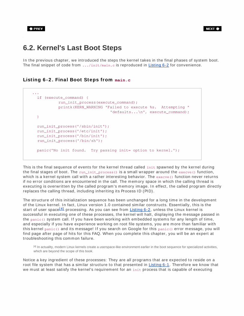
6.2. Kernel's Last Boot Steps
In the previous chapter, we introduced the steps the kernel takes in the final phases of system boot.The final snippet of code from .../init/main.c is reproduced in Listing 6-2 for convenience.
Listing 6-2. Final Boot Steps from main.c
... if (execute_command) { run_init_process(execute_command); printk(KERN_WARNING "Failed to execute %s. Attempting " "defaults...\n", execute_command); }
run_init_process("/sbin/init"); run_init_process("/etc/init"); run_init_process("/bin/init"); run_init_process("/bin/sh");
panic("No init found. Try passing init= option to kernel.");
This is the final sequence of events for the kernel thread called init spawned by the kernel duringthe final stages of boot. The run_init_process() is a small wrapper around the execve() function,which is a kernel system call with a rather interesting behavior. The execve() function never returnsif no error conditions are encountered in the call. The memory space in which the calling thread isexecuting is overwritten by the called program's memory image. In effect, the called program directlyreplaces the calling thread, including inheriting its Process ID (PID).
The structure of this initialization sequence has been unchanged for a long time in the developmentof the Linux kernel. In fact, Linux version 1.0 contained similar constructs. Essentially, this is thestart of user space[4] processing. As you can see from Listing 6-2, unless the Linux kernel issuccessful in executing one of these processes, the kernel will halt, displaying the message passed inthe panic() system call. If you have been working with embedded systems for any length of time,and especially if you have experience working on root file systems, you are more than familiar withthis kernel panic() and its message! If you search on Google for this panic() error message, you willfind page after page of hits for this FAQ. When you complete this chapter, you will be an expert attroubleshooting this common failure.
[4] In actuality, modern Linux kernels create a userspace-like environment earlier in the boot sequence for specialized activities,
which are beyond the scope of this book.
Notice a key ingredient of these processes: They are all programs that are expected to reside on aroot file system that has a similar structure to that presented in Listing 6-1. Therefore we know thatwe must at least satisfy the kernel's requirement for an init process that is capable of executing

within its own environment.
In looking at Listing 6-2, this means that at least one of the run_init_process() function calls mustsucceed. You can see that the kernel tries to execute one of four programs in the order in which theyare encountered. As you can see from the listing, if none of these four programs succeeds, thebooting kernel issues the dreaded panic() function call and dies right there. Remember, this snippetof code from .../init/main.c is executed only once on bootup. If it does not succeed, the kernel cando little but complain and halt, which it does through the panic() function call.
6.2.1. First User Space Program
On most Linux systems, /sbin/init is spawned by the kernel on boot. This is why it is attempted firstfrom Listing 6-2. Effectively, this becomes the first user space program to run. To review, this is thesequence:
1. Mount the root file system
2. Spawn the first user space program, which, in this discussion, becomesinit
In our example minimal root file system from Listing 6-2, the first three attempts at spawning a userspace process would fail because we did not provide an executable file called init anywhere on thefile system. Recall from Listing 6-1 that we had a soft link called sh that pointed back to busybox. Youshould now realize the purpose for that soft link: It causes busybox to be executed by the kernel asthe initial process, while also satisfying the common requirement for a shell executable fromuserspace.[5]
[5] When busybox is invoked via the sh symbolic link, it spawns a shell. We cover this in detail in Chapter 11.
6.2.2. Resolving Dependencies
It is not sufficient to simply include an executable such as init on your file system and expect it toboot. For every process you place on your root file system, you must also satisfy its dependencies.Most processes have two categories of dependencies: those that are needed to resolve unresolvedreferences within a dynamically linked executable, and external configuration or data files that anapplication might need. We have a tool to find the former, but the latter can be supplied only by atleast a cursory understanding of the application in question.
An example will help make this clear. The init process is a dynamically linked executable. To runinit, we need to satisfy its library dependencies. A tool has been developed for this purpose: ldd. Tounderstand what libraries a given application requires, simply run your cross-version of ldd on thebinary:
$ ppc_4xxFP-ldd init libc.so.6 => /opt/eldk/ppc_4xxFP/lib/libc.so.6 ld.so.1 => /opt/eldk/ppc_4xxFP/lib/ld.so.1 $

From this ldd output, we can see that the PowerPC init executable in this example is dependent ontwo libraries. These are the standard C library (libc.so.6) and the Linux dynamic loader (ld.so.1).
To satisfy the second category of dependencies for an executable, the configuration and data filesthat it might need, there is little substitute for some knowledge about how the subsystem works. Forexample, init expects to read its operational configuration from a data file called inittab located on/etc. Unless you are using a tool that has this knowledge built in, such as those described in theearlier Section 6.1.6, "Automated File System Build Tools," you must supply that knowledge.
6.2.3. Customized Initial Process
It is worth noting that the developer can control which initial process is executed at startup. This isdone by a kernel command line parameter. It is hinted at in Listing 6-2 by the text contained withinthe panic() function call. Building on our kernel command line from Chapter 5, here is how it mightlook with a developer-specified init process:
console=ttyS0,115200 ip=bootp root=/dev/nfs init=/sbin/myinit
Specifying init= in the kernel command line in this way, you must provide a binary executable onyour root file system in the /sbin directory called myinit. This would be the first process to gaincontrol at the completion of the kernel's boot process.

6.3. The Init Process
Unless you are doing something highly unusual, you will never need to provide a customized initialprocess because the capabilities of the standard init process are very flexible. The init program,together with a family of startup scripts that we examine shortly, implement what is commonly calledSystem V Init, from the original UNIX System V that used this schema. We now examine thispowerful system configuration and control utility.
We saw in the previous section that init is the first user space process spawned by the kernel aftercompletion of the boot process. As you will learn, every process in a running Linux system has achild-parent relationship with another process running in the system. init is the ultimate parent of alluser space processes in a Linux system. Furthermore, init provides the default set of environmentparameters for all other processes to inherit, including such things as PATH and CONSOLE.
Its primary role is to spawn additional processes under the direction of a special configuration file.This configuration file is usually stored as /etc/inittab. init has the concept of a runlevel. A runlevelcan be thought of as a system state. Each runlevel is defined by the services enabled and programsspawned upon entry to that runlevel.
init can exist in a single runlevel at any given time. Runlevels used by init include runlevels from 0to 6 and a special runlevel called S. Runlevel 0 instructs init to halt the system, while runlevel 6results in a system reboot. For each run-level, a set of startup and shutdown scripts is usuallyprovided that define the action a system should take for each runlevel. Actions to perform for a givenrunlevel are determined by the /etc/inittab configuration file, described shortly.
Several of the runlevels have been reserved for specific purposes in many distributions. Table 6-2details the runlevels and their purpose in common use in many Linux distributions.
Table 6-2. Runlevels
Runlevel Purpose
0 System shutdown (halt)
1 Single-user system configurationfor maintenance
2 User defined
3 General purpose multiuserconfiguration
4 User defined
5 Multiuser with graphical userinterface on startup

Runlevel Purpose
6 System restart (reboot)
The runlevel scripts are commonly found under a directory called /etc/rc.d/init.d. Here you willfind most of the scripts that enable and disable individual services. Services can be configuredmanually, by invoking the script and passing one of the appropriate arguments to the script, such asstart, stop, or restart. Listing 6-3 displays an example of restarting the nfs service.
Listing 6-3. NFS Restart
$ /etc/rc.d/init.d/nfs restartShutting down NFS mountd: [ OK ]Shutting down NFS daemon: [ OK ]Shutting down NFS quotas: [ OK ]Shutting down NFS services: [ OK ]Starting NFS services: [ OK ]Starting NFS quotas: [ OK ]Starting NFS daemon: [ OK ]Starting NFS mountd: [ OK ]
If you have spent any time with a desktop Linux distribution such as Red Hat or Fedora, you haveundoubtedly seen lines like this during system startup.
A runlevel is defined by the services that are enabled at that runlevel. Most Linux distributionscontain a directory structure under /etc that contains symbolic links to the service scripts in/etc/rc.d/init.d. These runlevel directories are typically rooted at /etc/rc.d. Under this directory,you will find a series of runlevel directories that contain startup and shutdown specifications for eachrunlevel. init simply executes these scripts upon entry and exit from a runlevel. The scripts definethe system state, and inittab instructs init on which scripts to associate with a given runlevel.Listing 6-4 contains the directory structure beneath /etc/rc.d that drives the runlevel startup andshutdown behavior upon entry to or exit from the specified runlevel, respectively.
Listing 6-4. Runlevel Directory Structure

$ ls -l /etc/rc.dtotal 96drwxr-xr-x 2 root root 4096 Oct 20 10:19 init.d-rwxr-xr-x 1 root root 2352 Mar 16 2004 rcdrwxr-xr-x 2 root root 4096 Mar 22 2005 rc0.ddrwxr-xr-x 2 root root 4096 Mar 22 2005 rc1.ddrwxr-xr-x 2 root root 4096 Mar 22 2005 rc2.ddrwxr-xr-x 2 root root 4096 Mar 22 2005 rc3.ddrwxr-xr-x 2 root root 4096 Mar 22 2005 rc4.ddrwxr-xr-x 2 root root 4096 Mar 22 2005 rc5.ddrwxr-xr-x 2 root root 4096 Mar 22 2005 rc6.d-rwxr-xr-x 1 root root 943 Dec 31 16:36 rc.local-rwxr-xr-x 1 root root 25509 Jan 11 2005 rc.sysinit
Each of the runlevels is defined by the scripts contained in the rcN.d, where N is the runlevel. Insideeach rcN.d directory, you will find numerous symlinks arranged in a specific order. These symboliclinks start with either a K or an S. Those beginning with S point to service scripts, which are invokedwith startup instructions; those starting with a K point to service scripts that are invoked withshutdown instructions. An example with a very small number of services might look like Listing 6-5.
Listing 6-5. Example Runlevel Directory
lrwxrwxrwx 1 root root 17 Nov 25 2004 S10network -> ../init.d/networklrwxrwxrwx 1 root root 16 Nov 25 2004 S12syslog -> ../init.d/sysloglrwxrwxrwx 1 root root 16 Nov 25 2004 S56xinetd -> ../init.d/xinetdlrwxrwxrwx 1 root root 16 Nov 25 2004 K50xinetd -> ../init.d/xinetdlrwxrwxrwx 1 root root 16 Nov 25 2004 K88syslog -> ../init.d/sysloglrwxrwxrwx 1 root root 17 Nov 25 2004 K90network -> ../init.d/network
In this example, we are instructing the startup scripts to start three services upon entry to thisfictitious runlevel: network, syslog, and xinetd. Because the S* scripts are ordered with a numerictag, they will be started in this order. In a similar fashion, when exiting this runlevel, three serviceswill be terminated: xinetd, syslog, and network. In a similar fashion, these services will beterminated in the order presented by the two-digit number following the K in the symlink filename. Inan actual system, there would undoubtedly be many more entries. You can include your own entriesfor your own custom applications, too.
The top-level script that executes these service startup and shutdown scripts is defined in the initconfiguration file, which we now examine.
6.3.1. inittab
When init is started, it reads the system configuration file /etc/inittab. This file contains directivesfor each runlevel, as well as directives that apply to all run-levels. This file and init's behavior arewell documented in man pages on most Linux workstations, as well as by several books covering

system administration. We do not attempt to duplicate those works; we focus on how a developermight configure inittab for an embedded system. For a detailed explanation of how inittab andinit work together, view the man page on most Linux workstations by typing man init and maninittab.
Let's take a look at a typical inittab for a simple embedded system. Listing 6-6 contains a simpleinittab example for a system that supports a single runlevel as well as shutdown and reboot.
Listing 6-6. Simple Example inittab
# /etc/inittab
# The default runlevel (2 in this example) id:2:initdefault:
# This is the first process (actually a script) to be run. si::sysinit:/etc/rc.sysinit
# Execute our shutdown script on entry to runlevel 0 l0:0:wait:/etc/init.d/sys.shutdown
# Execute our normal startup script on entering runlevel 2 l2:2:wait:/etc/init.d/runlvl2.startup
# This line executes a reboot script (runlevel 6) l6:6:wait:/etc/init.d/sys.reboot
# This entry spawns a login shell on the console # Respawn means it will be restarted each time it is killed con:2:respawn:/bin/sh
This very simple[6] inittab script describes three individual runlevels. Each run-level is associatedwith a script, which must be created by the developer for the desired actions in each runlevel. Whenthis file is read by init, the first script to be executed is /etc/rc.sysinit. This is denoted by thesysinit tag. Then init enters runlevel 2, and executes the script defined for runlevel 2. From thisexample, this would be /etc/init.d/runlvl2.startup. As you might guess from the :wait: tag inListing 6-6, init waits until the script completes before continuing. When the runlevel 2 scriptcompletes, init spawns a shell on the console (through the /bin/sh symbolic link), as shown in thelast line of Listing 6-6. The respawn keyword instructs init to restart the shell each time it detectsthat it has exited. Listing 6-7 shows what it looks like during boot.
[6] This inittab is a nice example of a small, purpose-built embedded system.
Listing 6-7. Example Startup Messages

...VFS: Mounted root (nfs filesystem).Freeing init memory: 304KINIT: version 2.78 bootingThis is rc.sysinitINIT: Entering runlevel: 2This is runlvl2.startup
#
The startup scripts in this example do nothing except announce themselves for illustrative purposes.Of course, in an actual system, these scripts enable features and services that do useful work! Giventhe simple configuration in this example, you would enable the services and applications for yourparticular widget in the /etc/init.d/runlvl2.startup script and do the reversedisable yourapplications, services, and devicesin your shutdown and/or reboot scripts. In the next section, welook at some typical system configurations and the required entries in the startup scripts to enablethese configurations.
6.3.2. Example Web Server Startup Script
Although simple, this example startup script is designed to illustrate the mechanism and guide you indesigning your own system startup and shutdown behavior. This example is based on busybox, whichhas a slightly different initialization behavior than init. These differences are covered in detail inChapter 11.
In a typical embedded appliance that contains a web server, we might want several servers availablefor maintenance and remote access. In this example, we enable servers for HTTP and Telnet access(via inetd). Listing 6-8 contains a simple rc.sysinit script for our hypothetical web server appliance.
Listing 6-8. Web Server rc.sysinit
#!/bin/sh
echo "This is rc.sysinit"
busybox mount -t proc none /proc
# Load the system loggers syslogd klogd
# Enable legacy PTY support for telnetd busybox mkdir /dev/pts busybox mknod /dev/ptmx c 5 2 busybox mount -t devpts devpts /dev/pts

In this simple initialization script, we first enable the proc file system. The details of this usefulsubsystem are covered in Chapter 9. Next we enable the system loggers so that we can capturesystem information during operation. This is especially useful when things go wrong. The last entriesenable support for the UNIX PTY subsystem, which is required for the implementation of the Telnetserver used for this example.
Listing 6-9 contains the commands in the runlevel 2 startup script. This script contains the commandsto enable any services we want to have operational for our appliance.
Listing 6-9. Example Runlevel 2 Startup Script
#!/bin/sh
echo "This is runlvl2.startup"
echo "Starting Internet Superserver" inetd
echo "Starting web server" webs &
Notice how simple this runlevel 2 startup script actually is. First we enable the so-called Internetsuperserver inetd, which intercepts and spawns services for common TCP/IP requests. In ourexample, we enabled Telnet services through a configuration file called /etc/inetd.conf. Then weexecute the web server, here called webs. That's all there is to it. Although minimal, this is a workingconfiguration for Telnet and web services.
To complete this configuration, you might supply a shutdown script (refer back to Listing 6-6), which,in this case, would terminate the web server and the Internet superserver before system shutdown.In our example scenario, that is sufficient for a clean shutdown.

6.4. Initial RAM Disk
The Linux kernel contains a mechanism to mount an early root file system to perform certain startup-related system initialization and configuration. This mechanism is known as the initial RAM disk, orsimply initrd. Support for this functionality must be compiled into the kernel. This kernel configurationoption is found under Block Devices, RAM disk support in the kernel configuration utility. Figure 6-1shows an example of the configuration for initrd.
Figure 6-1. Linux kernel configuration utility
[View full size image]
6.4.1. Initial RAM Disk Purpose
The initial RAM disk is a small self-contained root file system that usually contains directives to loadspecific device drivers before the completion of the boot cycle. In Linux workstation distributions suchas Red Hat and Fedora Core, an initial RAM disk is used to load the device drivers for the EXT3 filesystem before mounting the real root file system. An initrd is frequently used to load a device driver

that is required in order to access the real root file system.
6.4.2. Booting with initrd
To use the initrd functionality, the bootloader gets involved on most architectures to pass theinitrd image to the kernel. A common scenario is that the bootloader loads a compressed kernelimage into memory and then loads an initrd image into another section of available memory. Indoing so, it becomes the bootloader's responsibility to pass the load address of the initrd image tothe kernel before passing control to it. The exact mechanism differs depending on the architecture,bootloader, and platform implementation. However, the kernel must know where the initrd image islocated so it can load it.
Some architectures and platforms construct a single composite binary image. This scheme is usedwhen the bootloader does not have specific Linux support for loading initrd images. In this case, thekernel and initrd image are simply concatenated together. You will find reference to this type ofcomposite image in the kernel makefiles as bootpImage. Presently, this is used only for armarchitecture.
So how does the kernel know where to find the initrd image? Unless there is some special magic inthe bootloader, it is usually sufficient simply to pass the initrd image start address and size to thekernel via the kernel command line. Here is an example of a kernel command line for a popular ARM-based reference board containing the TI OMAP 5912 processor.
console=ttyS0,115200 root=/dev/nfs \ nfsroot=192.168.1.9:/home/chris/sandbox/omap-target \ initrd=0x10800000,0x14af47
The previous kernel command line has been separated into several lines to fit in the space provided.In actual practice, it is a single line, with the individual elements separated by spaces. This kernelcommand line defines the following kernel behavior:
Specify a single console on device ttyS0 at 115 kilobaud
Mount a root file system via NFS, the network file system
Find the NFS root file system on host 192.168.1.9
(from directory /home/chris/sandbox/omap-target)
Load and mount an initial ramdisk from physical memory location
0x10800000, which has a size of 0x14AF47 (1,355,591 bytes)
One additional note regarding this example: Almost universally, the initrd image is compressed. Thesize specified on the kernel command line is the size of the compressed image.
6.4.3. Bootloader Support for initrd

Let's look at a simple example based on the popular U-Boot bootloader running on an ARM processor.This bootloader has been designed with Linux kernel support. Using U-Boot, it is easy to include aninitrd image with the kernel image. Listing 6-10 examines a typical boot sequence containing aninitial ramdisk image.
Listing 6-10. Booting Kernel with Ramdisk Support
# tftpboot 0x10000000 kernel-uImage...Load address: 0x10000000Loading: ############################ doneBytes transferred = 1069092 (105024 hex)
# tftpboot 0x10800000 initrd-uboot...Load address: 0x10800000Loading: ########################################### doneBytes transferred = 282575 (44fcf hex)
# bootm 0x10000000 0x10800040Uncompressing kernel.................done....RAMDISK driver initialized: 16 RAM disks of 16384K size 1024 blocksize...RAMDISK: Compressed image found at block 0VFS: Mounted root (ext2 filesystem).Greetings: this is linuxrc from Initial RAMDiskMounting /proc filesystem
BusyBox v1.00 (2005.03.14-16:37+0000) Built-in shell (ash)Enter 'help' for a list of built-in commands.
# (<<<< Busybox command prompt)
Here in Listing 6-10, we get a glimpse of the U-Boot bootloader, which we examine in more detail inthe next chapter. The tftpboot command causes U-Boot to download the kernel image from a tftpserver. The kernel image is downloaded and placed into the base of this target system's memory atthe 256MB address (0x10000000 hex[7]). Then a second image, the initial ramdisk image, isdownloaded from a tftp server into memory at a higher memory address (256MB + 8MB, in thisexample). Finally, we issue the U-Boot bootm command, which is the "boot from memory" command.The bootm command takes two arguments: the address of the Linux kernel image, optionally followedby an address representing the location of the initial ramdisk image.
[7] It just so happens that on this particular board, our physical SDRAM starts at 256MB.
Take special note of one feature of the U-Boot bootloader. It fully supports loading kernel andramdisk images over an Ethernet connection. This is a very useful development configuration. Youcan get a kernel and ramdisk image onto your board in other ways as well. You can flash them intoyour Flash memory using a hardware-based flash programming tool, or you can use a serial port and

download the kernel and file system images via RS-232. However, because these images are typicallylarge (a kernel can be about a megabyte, and a ramdisk can be tens of megabytes), you will save asignificant amount of engineering time if you invest in this Ethernet-based tftp download method.Whatever bootloader you choose, make sure it supports network download of development images.
6.4.4. initrd Magic: linuxrc
When the kernel boots, it detects the presence of the initrd image, and copies the compressedbinary file from the specified physical location in RAM into a proper kernel ramdisk and mounts it asthe root file system. The magic of the initrd comes from the contents of a special file within theinitrd image. When the kernel mounts the initial ramdisk, it looks for a specific file called linuxrc. Ittreats this file as a script file and proceeds to execute the commands contained therein. Thismechanism enables the system designer to specify the behavior of initrd. Listing 6-11 contains asample linuxrc file.
Listing 6-11. Example linuxrc File
#!/bin/sh
echo 'Greetings: this is 'linuxrc' from Initial Ramdisk'echo 'Mounting /proc filesystem'mount -t proc /proc /proc
busybox sh
In practice, this file would contain directives required before we mount the real root file system. Oneexample might be to load CompactFlash drivers to obtain a real root file system from a CompactFlashdevice. For purposes of this example, we simply spawn a busybox shell and halt the boot process forexamination. You can see the # command prompt from Listing 6-10 resulting from this busybox shell.If one were to type the exit command here, the kernel would continue its boot process untilcomplete.
After the kernel copies the ramdisk from physical memory into a kernel ramdisk, it returns thisphysical memory back to the available memory pool. You can think of this as transferring the initrdimage from physical memory at the hard-coded address into the kernel's own virtual memory (in theform of a kernel ramdisk device).
One last comment about Listing 6-11: The mount command in which the /proc file system is mountedseems redundant in its use of the word proc. This command would also work:
mount -t proc none /proc
Notice that the device field of the mount command has been changed to none. The mount commandignores the device field because no physical device is associated with the proc file system. The -tproc is enough to instruct mount to mount the /proc file system on the /proc mount point. I use theformer invocation as a mental reminder that we are actually mounting the kernel pseudo device (the

/proc file system) on /proc. The mount command ignores this argument. Use the method that youprefer.
6.4.5. The initrd Plumbing
As part of the Linux boot process, the kernel must locate and mount a root file system. Late in theboot process, the kernel decides what and where to mount in a function called prepare_namespace().If initrd support is enabled in the kernel, as illustrated in Figure 6-1, and the kernel command line isso configured, the kernel decompresses the compressed initrd image from physical memory andeventually copies the contents of this file into a ramdisk device (/dev/ram). At this point, we have aproper file system on a kernel ramdisk. After the file system has been read into the ramdisk, thekernel effectively mounts this ramdisk device as its root file system. Finally, the kernel spawns akernel thread to execute the linuxrc file on the initrd image.[8]
[8] Out of necessity (space), this is a very simplified description of the sequence of events. The actual mechanism is similar in
concept, but several significant details are omitted for clarity. You are encouraged to consult the kernel source code for more
details. See .../init/main.c and .../init/do_mounts*.c.
When the linuxrc script has completed execution, the kernel unmounts the initrd and proceeds withthe final stages of system boot. If the real root device has a directory called /initrd, Linux mountsthe initrd file system on this path (in this context, called a mount point). If this directory does notexist in the final root file system, the initrd image is simply discarded.
If the kernel command line contains a root= parameter specifying a ramdisk (root=/dev/ram0, forexample), the previously described initrd behavior changes in two important ways. First, theprocessing of the linuxrc executable is skipped. Second, no attempt is made to mount another filesystem as root. This means that you can have a Linux system with initrd as the only root filesystem. This is useful for minimal system configurations in which the only root file system is theramdisk. Placing /dev/ram0 on the kernel command line allows the full system initialization tocomplete with the initrd as the final root file system.
6.4.6. Building an initrd Image
Constructing a suitable root file system image is one of the more challenging aspects of embeddedsystems. Creating a proper initrd image is even more challenging because it needs to be small andspecialized. For this section, we examine initrd requirements and file system contents.
Listing 6-12 was produced by running the tree utility on our example initrd image from this chapter.
Listing 6-12. Contents of Example initrd

.|-- bin| |-- busybox| |-- echo -> busybox| |-- mount -> busybox| '-- sh -> busybox|-- dev| |-- console| |-- ram0| '-- ttyS0|-- etc|-- linuxrc'-- proc
4 directories, 8 files
As you can see, it is very small indeed; it takes up a little more than 500KB in uncompressed form.Since it is based on busybox, it has many capabilities. Because busybox is statically linked, it has nodependencies on any system libraries. You will learn more about busybox in Chapter 11.

6.5. Using initramfs
initramfs is a relatively new (Linux 2.6) mechanism for executing early user space programs. It isconceptually similar to initrd, as described in the previous section. Its purpose is also similar: toenable loading of drivers that might be required before mounting the real root file system. However,it differs in significant ways from the initrd mechanism.
The technical implementation details differ significantly between initrd and initramfs. For example,initramfs is loaded before the call to do_basic_setup(),[9] which provides a mechanism for loadingfirmware for devices before its driver has been loaded. For more details, the Linux kerneldocumentation for this subsystem is relatively up-to-date. See
[9] do_basic_setup is called from .../init/main.c and calls do_initcalls(). This causes driver module initialization
routines to be called. This was described in detail in Chapter 5 and shown in Listing 5-10.
.../Documentation/filesystems/ramfs-rootfs-initramfs.txt.
From a practical perspective, initramfs is much easier to use. initramfs is a cpio archive, whereasinitrd is a gzipped file system image. This simple difference contributes to the easy of use ofinitramfs. It is integrated into the Linux kernel source tree and is built automatically when you buildthe kernel image. Making changes to it is far easier than building and loading a new initrd image.Listing 6-13 shows the contents of the Linux kernel .../usr directory, where the initramfs image isbuilt. The contents of Listing 6-13 are shown after a kernel has been built.
Listing 6-13. Kernel initramfs Build Directory
$ ls -ltotal 56-rw-rw-r-- 1 chris chris 834 Mar 25 11:13 built-in.o-rwxrwxr-x 1 chris chris 11512 Mar 25 11:13 gen_init_cpio-rw-rw-r-- 1 chris chris 10587 Oct 27 2005 gen_init_cpio.c-rw-rw-r-- 1 chris chris 512 Mar 25 11:13 initramfs_data.cpio-rw-rw-r-- 1 chris chris 133 Mar 25 11:13 initramfs_data.cpio.gz-rw-rw-r-- 1 chris chris 786 Mar 25 11:13 initramfs_data.o-rw-rw-r-- 1 chris chris 1024 Oct 27 2005 initramfs_data.S-rw-rw-r-- 1 chris chris 113 Mar 25 11:13 initramfs_list-rw-rw-r-- 1 chris chris 1619 Oct 27 2005 Kconfig-rw-rw-r-- 1 chris chris 2048 Oct 27 2005 Makefile
The file initramfs_list contains a list of files that will be included in the initramfs archive. Thedefault for recent Linux kernels looks like this:
dir /dev 0755 0 0

nod /dev/console 0600 0 0 c 5 1dir /root 0700 0 0
This produces a small default directory structure containing the /root and /dev top-level directories,as well as a single device node representing the console. Add to this file to build your own initramfs.You can also specify a source for your initramfs files via the kernel-configuration facility. EnableINITRAMFS_SOURCE in your kernel configuration and point it to a location on your developmentworkstation; the kernel build system will use those files as the source for your initramfs image.
The final output of this build directory is the initramfs_data_cpio.gz file. This is a compressedarchive containing the files you specified (either through the initramfs_list or via theINITRAMFS_SOURCE kernel-configuration option). This archive is linked into the final kernel image. Thisis another advantage of initramfs over initrd: There is no need to load a separate initrd image atboot time, as is the case with initrd.

6.6. Shutdown
Orderly shutdown of an embedded system is often overlooked in a design. Improper shutdown canaffect startup times and can even corrupt certain file system types. One of the more commoncomplaints using the EXT2 file system (the default in many desktop Linux distributions for severalyears) is the time it takes for an fsck (file system check) on startup after unplanned power loss.Servers with large disk systems can take on the order of hours to properly fsck through a collectionof large EXT2 partitions.
Each embedded project will likely have its own shutdown strategy. What works for one might ormight not work for another. The scale of shutdown can range from a full System V shutdown scheme,to a simple script to halt or reboot. Several Linux utilities are available to assist in the shutdownprocess, including the shutdown, halt, and reboot commands. Of course, these must be available foryour chosen architecture.
A shutdown script should terminate all userspace processes, which results in closing any open filesused by those processes. If init is being used, issuing the command init 0 halts the system. Ingeneral, the shutdown process first sends all processes the SIGTERM signal, to notify them that thesystem is shutting down. A short delay ensures that all processes have the opportunity to performtheir shutdown actions, such as closing files, saving state, and so on. Then all processes are sent theSIGKILL signal, which results in their termination. The shutdown process should attempt to unmountany mounted file systems and call the architecture-specific halt or reboot routines. The Linuxshutdown command in conjunction with init exhibits this behavior.

6.7. Chapter Summary
A root file system is required for all Linux systems. They can be difficult to build from scratchbecause of complex dependencies by each application.
The File System Hierarchy standard provides guidance to developers for laying out a file systemfor maximum compatibility and flexibility.
We presented a minimal file system as an example of how root file systems are created.
The Linux kernel's final boot steps define and control a Linux system's startup behavior. Severalmechanisms are available depending on your embedded Linux system's requirements.
The init process was presented in detail. This powerful system-configuration and control utilitycan serve as the basis for your own embedded Linux system. System initialization based oninit was presented, along with example startup script configurations.
Initial ramdisk is a Linux kernel feature to allow further startup behavior customization beforemounting a final root file system and spawning init. We presented the mechanism and exampleconfiguration for using this powerful feature.
initramfs simplifies the initial ramdisk mechanism, while providing similar early startupfacilities. It is easier to use, does not require loading a separate image, and is builtautomatically during each kernel build.
6.7.1. Suggestions for Additional Reading
File System Hierarchy StandardMaintained by freestandards.orgwww.pathname.com/fhs/
Boot Process, Init and ShutdownLinux Documentation Projecthttp://tldp.org/LDP/intro-linux/html/sect_04_02.html
Init man pageLinux Documentation Projecthttp://tldp.org/LDP/sag/html/init.html
A brief description of System V inithttp://docs.kde.org/en/3.3/kdeadmin/ksysv/what-is-sysv-init.html
Booting Linux: The History and the FutureWerner Almesbergerwww.almesberger.net/cv/papers/ols2k-9.ps


Chapter 7. BootloadersIn this chapter
Role of a Bootloader page 158
Bootloader Challenges page 159
A Universal Bootloader: Das U-Boot page 164
Porting U-Boot page 172
Other Bootloaders page 183
Chapter Summary page 186
Previous chapters have made reference to and even provided examples of bootloader operations. Acritical component of an embedded system, the bootloader provides the foundation from which theother system software is spawned. This chapter starts by examining the bootloader's role in asystem. We follow this with an introduction to some common features of bootloaders. Armed with thisbackground, we take a detailed look at a popular bootloader used for embedded systems. Weconclude this chapter by introducing a few of the more popular bootloaders.
Numerous bootloaders are in use today. It would be impractical in the given space to cover muchdetail on even the most popular ones. Therefore, we have chosen to explain concepts and useexamples based on one of the more popular bootloaders in the open source community for PowerPC,MIPS, ARM, and other architectures: the U-Boot bootloader.

7.1. Role of a Bootloader
When power is first applied to a processor board, many elements of hardware must be initializedbefore even the simplest program can run. Each architecture and processor has a set of predefinedactions and configurations, which include fetching some initialization code from an on-board storagedevice (usually Flash memory). This early initialization code is part of the bootloader and isresponsible for breathing life into the processor and related hardware components.
Most processors have a default address from which the first bytes of code are fetched uponapplication of power and release of reset. Hardware designers use this information to arrange thelayout of Flash memory on the board and to select which address range(s) the Flash memoryresponds to. This way, when power is first applied, code is fetched from a well-known and predictableaddress, and software control can be established.
The bootloader provides this early initialization code and is responsible for initializing the board sothat other programs can run. This early initialization code is almost always written in the processor'snative assembly language. This fact alone presents many challenges, some of which we examinehere.
Of course, after the bootloader has performed this basic processor and platform initialization, itsprimary role becomes booting a full-blown operating system. It is responsible for locating, loading,and passing execution to the primary operating system. In addition, the bootloader might haveadvanced features, such as the capability to validate an OS image, the capability to upgrade itself oran OS image, and the capability to choose from among several OS images based on a developer-defined policy. Unlike the traditional PC-BIOS model, when the OS takes control, the bootloader isoverwritten and ceases to exist.[1]
[1] Some embedded designs protect the bootloader and provide callbacks to bootloader routines, but this is almost never a good
design approach. Linux is far more capable than bootloaders, so there is often little point in doing so.

7.2. Bootloader Challenges
Even a simple "Hello World" program written in C requires significant hardware and softwareresources. The application developer does not need to know or care much about these detailsbecause the C runtime environment transparently provides this infrastructure. A bootloaderdeveloper has no such luxury. Every resource that a bootloader requires must be carefully initializedand allocated before it is used. One of the most visible examples of this is Dynamic Random AccessMemory (DRAM).
7.2.1. DRAM Controller
DRAM chips cannot be directly read from or written to like other microprocessor bus resources. Theyrequire specialized hardware controllers to enable read and write cycles. To further complicatematters, DRAM must be constantly refreshed or the data contained within will be lost. Refresh isaccomplished by sequentially reading each location in DRAM in a systematic manner and within thetiming specifications set forth by the DRAM manufacturer. Modern DRAM chips support many modesof operation, such as burst mode and dual data rate for high-performance applications. It is theDRAM controller's responsibility to configure DRAM, keep it refreshed within the manufacturer'stiming specifications, and respond to the various read and write commands from the processor.
Setting up a DRAM controller is the source of much frustration for the newcomer to embeddeddevelopment. It requires detailed knowledge of DRAM architecture, the controller itself, the specificDRAM chips being used, and the overall hardware design. Though this is beyond the scope of thisbook, the interested reader can learn more about this important concept by referring to thereferences at the end of this chapter. Appendix D, "SDRAM Interface Considerations," provides morebackground on this important topic.
Very little can happen in an embedded system until the DRAM controller and DRAM itself have beenproperly initialized. One of the first things a bootloader must do is to enable the memory subsystem.After it is initialized, memory can be used as a resource. In fact, one of the first actions manybootloaders perform after memory initialization is to copy themselves into DRAM for faster execution.
7.2.2. Flash Versus RAM
Another complexity inherent in bootloaders is that they are required to be stored in nonvolatilestorage but are usually loaded into RAM for execution. Again, the complexity arises from the level ofresources available for the bootloader to rely on. In a fully operational computer system running anoperating system such as Linux, it is relatively easy to compile a program and invoke it fromnonvolatile storage. The runtime libraries, operating system, and compiler work together to createthe infrastructure necessary to load a program from nonvolatile storage into memory and passcontrol to it. The aforementioned "Hello World" program is a perfect example. When compiled, it canbe loaded into memory and executed simply by typing the name of the executable (hello) on thecommand line (assuming, of course, that the executable exists somewhere on your PATH).

This infrastructure does not exist when a bootloader gains control upon power-on. Instead, thebootloader must create its own operational context and move itself, if required, to a suitable locationin RAM. Furthermore, additional complexity is introduced by the requirement to execute from a read-only medium.
7.2.3. Image Complexity
As application developers, we do not need to concern ourselves with the layout of a binary executablefile when we develop applications for our favorite platform. The compiler and binary utilities arepreconfigured to build a binary executable image containing the proper components needed for agiven architecture. The linker places startup (prologue) and shutdown (epilogue) code into the image.These objects set up the proper execution context for your application, which typically starts atmain() in your application.
This is absolutely not the case with a typical bootloader. When the bootloader gets control, there isno context or prior execution environment. In a typical system, there might not be any DRAM untilthe bootloader initializes the processor and related hardware. Consider what this means. In a typicalC function, any local variables are stored on the stack, so a simple function like the one in Listing 7-1is unusable.
Listing 7-1. Simple C function
int setup_memory_controller(board_info_t *p) { unsigned int *dram_controller_register = p->dc_reg;...
When a bootloader gains control on power-on, there is no stack and no stack pointer. Therefore, asimple C function similar to Listing 7-1 will likely crash the processor because the compiler willgenerate code to create and initialize the pointer dram_controller_register on the stack, which doesnot yet exist. The bootloader must create this execution context before any C functions are called.
When the bootloader is compiled and linked, the developer must exercise complete control over howthe image is constructed and linked. This is especially true if the bootloader is to relocate itself fromFlash to RAM. The compiler and linker must be passed a handful of parameters defining thecharacteristics and layout of the final executable image. Two primary characteristics conspire to addcomplexity to the final binary executable image.
The first characteristic that presents complexity is the need to organize the startup code in a formatcompatible with the processor's boot sequence. The first bytes of executable code must be at apredefined location in Flash, depending on the processor and hardware architecture. For example, theAMCC PowerPC 405GP processor seeks its first machine instructions from a hard-coded address of0xFFFF_FFFC. Other processors use similar methods with different details. Some processors areconfigurable at power-on to seek code from one of several predefined locations, depending onhardware configuration signals.
How does a developer specify the layout of a binary image? The linker is passed a linker description

file, also called a linker command script. This special file can be thought of as a recipe forconstructing a binary executable image. Listing 7-2 contains a snippet from an existing linkerdescription file in use in a popular bootloader, which we discuss shortly.
Listing 7-2. Linker Command ScriptReset Vector Placement
SECTIONS{ .resetvec 0xFFFFFFFC : { *(.resetvec) } = 0xffff...
A complete description of linker command scripts syntax is beyond the scope of this book. Theinterested reader is directed to the GNU LD manual referenced at the end of this chapter. Looking atListing 7-2, we see the beginning of the definition for the output section of the binary ELF image. Itdirects the linker to place the section of code called .resetvec at a fixed address in the output image,starting at location 0xFFFF_FFFC. Furthermore, it specifies that the rest of this section shall be filledwith all ones (0xFFFF.) This is because an erased Flash memory array contains all ones. Thistechnique not only saves wear and tear on the Flash memory, but it also significantly speeds upprogramming of that sector.
Listing 7-3 is the complete assembly language file from a recent U-Boot distribution that defines the.resetvec code section. It is contained in an assembly language file called.../cpu/ppc4xx/resetvec.S. Notice that this code section cannot exceed 4 bytes in length in amachine with only 32 address bits. This is because only a single instruction is defined in this section,no matter what configuration options are present.
Listing 7-3. Source Definition of .resetvec
/* Copyright MontaVista Software Incorporated, 2000 */#include <config.h> .section .resetvec, "ax"#if defined(CONFIG_440) b _start_440#else#if defined(CONFIG_BOOT_PCI) && defined(CONFIG_MIP405) b _start_pci#else b _start#endif#endif
This assembly language file is very easy to understand, even if you have no assembly language

programming experience. Depending on the particular configuration (as specified by the CONFIG_*macros), an unconditional branch instruction (b in PowerPC assembler syntax) is generated to theappropriate start location in the main body of code. This branch location is a 4-byte PowerPCinstruction, and as we saw in the snippet from the linker command script in Listing 7-2, this simplebranch instruction is placed in the absolute Flash address of 0xFFFF_FFFC in the output image. Asmentioned earlier, the PPC 405GP processor fetches its first instruction from this hard-coded address.This is how the first sequence of code is defined and provided by the developer for this particulararchitecture and processor combination.
7.2.4. Execution Context
The other primary reason for bootloader image complexity is the lack of execution context. When thesequence of instructions from Listing 7-3 starts executing (recall that these are the first machineinstructions after power-on), the resources available to the running program are nearly zero. Defaultvalues designed into the hardware ensure that fetches from Flash memory work properly and thatthe system clock has some default values, but little else can be assumed.[2] The reset state of eachprocessor is usually well defined by the manufacturer, but the reset state of a board is defined by thehardware designers.
[2] The details differ, depending upon architecture, processor, and details of the hardware design.
Indeed, most processors have no DRAM available at startup for temporary storage of variables or,worse, for a stack that is required to use C program calling conventions. If you were forced to write a"Hello World" program with no DRAM and, therefore, no stack, it would be quite different from thetraditional "Hello World" example.
This limitation places significant challenges on the initial body of code designed to initialize thehardware. As a result, one of the first tasks the bootloader performs on startup is to configureenough of the hardware to enable at least some minimal amount of RAM. Some processors designedfor embedded use have small amounts of on-chip static RAM available. This is the case with the PPC405GP we've been discussing. When RAM is available, a stack can be allocated using part of thatRAM, and a proper context can be constructed to run higher-level languages such as C. This allowsthe rest of the processor and platform initialization to be written in something other than assemblylanguage.

7.3. A Universal Bootloader: Das U-Boot
Many open-source and commercial bootloaders are available, and many more one-of-a-kind home-grown designs are in widespread use today. Most of these have some level of commonality offeatures. For example, all of them have some capability to load and execute other programs,particularly an operating system. Most interact with the user through a serial port. Support forvarious networking subsystems (such as Ethernet) is less common but a very powerful feature.
Many bootloaders are specific to a particular architecture. The capability of a bootloader to support awide variety of architectures and processors can be an important feature to larger developmentorganizations. It is not uncommon for a single development organization to have multiple processorsspanning more than one architecture. Investing in a single bootloader across multiple platformsultimately results in lower development costs.
In this section, we study an existing bootloader that has become very popular in the embedded Linuxcommunity. The official name for this bootloader is Das U-Boot. It is maintained by Wolfgang Denkand hosted on SourceForge at http://u-boot.sourceforge.net/. U-Boot has support for multiplearchitectures and has a large following of embedded developers and hardware manufacturers whohave adopted it for use in their projects and have contributed to its development.
7.3.1. System Configuration: U-Boot
For a bootloader to be useful across many processors and architectures, some method of configuringthe bootloader is necessary. As with the Linux kernel itself, configuration of a bootloader is done atcompile time. This method significantly reduces the complexity of the bootloader, which, in itself, isan important characteristic.
In the case of U-Boot, board-specific configuration is driven by a single header file specific to thetarget platform, and a few soft links in the source tree that select the correct subdirectories based ontarget board, architecture, and CPU. When configuring U-Boot for one of its supported platforms,issue this command:
$ make <platform>_config
Here, platform is one of the many platforms supported by U-Boot. These platform-configurationtargets are listed in the top level U-Boot makefile. For example, to configure for the Spectrum DigitalOSK, which contains a TI OMAP 5912 processor, issue this command:
$ make omap5912osk_config
This configures the U-Boot source tree with the appropriate soft links to select ARM as the targetarchitecture, the ARM926 core, and the 5912 OSK as the target platform.

The next step in configuring U-Boot for this platform is to edit the configuration file specific to thisboard. This file is found in the U-Boot ../include/configs subdirectory and is called omap5912osk.h.The README file that comes with the U-Boot distribution describes the details of configuration and isthe best source for this information.
Configuration of U-Boot is done using configuration variables defined in a board-specific header file.Configuration variables have two forms. Configuration options are selected using macros in the formof CONFIG_XXXX. Configuration settings are selected using macros in the form of CFG_XXXX. In general,configuration options (CONFIG_XXX) are user configurable and enable specific U-Boot operationalfeatures. Configuration settings (CFG_XXX) are usually hardware specific and require detailedknowledge of the underlying processor and/or hardware platform. Board-specific U-Boot configurationis driven by a header file dedicated to that specific platform that contains configuration options andsettings appropriate for the underlying platform. The U-Boot source tree includes a directory wherethese board-specific configuration header files reside. They can be found in .../include/configsfrom the top-level U-Boot source directory.
Numerous features and modes of operation can be selected by adding definitions to the board-configuration file. Listing 7-4 contains a partial configuration header file for a fictitious board based onthe PPC 405GP processor.
Listing 7-4. Partial U-Boot Board-Configuration Header File
#define CONFIG_405GP /* Processor definition */#define CONFIG_4XX /* Sub-arch specification, 4xx family */
#define CONFIG_SYS_CLK_FREQ 33333333 /* PLL Frequency */#define CONFIG_BAUDRATE 9600#define CONFIG_PCI /* Enable support for PCI */...#define CONFIG_COMMANDS (CONFIG_CMD_DFL | CFG_CMD_DHCP)...#define CFG_BASE_BAUD 691200
/* The following table includes the supported baudrates */#define CFG_BAUDRATE_TABLE \ {1200, 2400, 4800, 9600, 19200, 38400, 57600, 115200, 230400}
#define CFG_LOAD_ADDR 0x100000 /* default load address */.../* Memory Bank 0 (Flash Bank 0) initialization */#define CFG_EBC_PB0AP 0x9B015480#define CFG_EBC_PB0CR 0xFFF18000
#define CFG_EBC_PB1AP 0x02815480#define CFG_EBC_PB1CR 0xF0018000...
Listing 7-4 gives an idea of how U-Boot itself is configured for a given board. An actual board-configuration file can contain hundreds of lines similar to those found here. In this example, you can
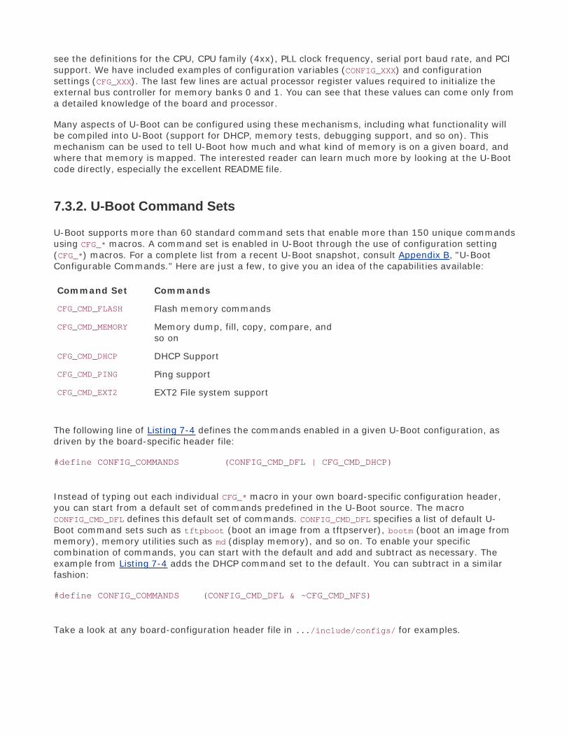
see the definitions for the CPU, CPU family (4xx), PLL clock frequency, serial port baud rate, and PCIsupport. We have included examples of configuration variables (CONFIG_XXX) and configurationsettings (CFG_XXX). The last few lines are actual processor register values required to initialize theexternal bus controller for memory banks 0 and 1. You can see that these values can come only froma detailed knowledge of the board and processor.
Many aspects of U-Boot can be configured using these mechanisms, including what functionality willbe compiled into U-Boot (support for DHCP, memory tests, debugging support, and so on). Thismechanism can be used to tell U-Boot how much and what kind of memory is on a given board, andwhere that memory is mapped. The interested reader can learn much more by looking at the U-Bootcode directly, especially the excellent README file.
7.3.2. U-Boot Command Sets
U-Boot supports more than 60 standard command sets that enable more than 150 unique commandsusing CFG_* macros. A command set is enabled in U-Boot through the use of configuration setting(CFG_*) macros. For a complete list from a recent U-Boot snapshot, consult Appendix B, "U-BootConfigurable Commands." Here are just a few, to give you an idea of the capabilities available:
Command Set Commands
CFG_CMD_FLASH Flash memory commands
CFG_CMD_MEMORY Memory dump, fill, copy, compare, andso on
CFG_CMD_DHCP DHCP Support
CFG_CMD_PING Ping support
CFG_CMD_EXT2 EXT2 File system support
The following line of Listing 7-4 defines the commands enabled in a given U-Boot configuration, asdriven by the board-specific header file:
#define CONFIG_COMMANDS (CONFIG_CMD_DFL | CFG_CMD_DHCP)
Instead of typing out each individual CFG_* macro in your own board-specific configuration header,you can start from a default set of commands predefined in the U-Boot source. The macroCONFIG_CMD_DFL defines this default set of commands. CONFIG_CMD_DFL specifies a list of default U-Boot command sets such as tftpboot (boot an image from a tftpserver), bootm (boot an image frommemory), memory utilities such as md (display memory), and so on. To enable your specificcombination of commands, you can start with the default and add and subtract as necessary. Theexample from Listing 7-4 adds the DHCP command set to the default. You can subtract in a similarfashion:
#define CONFIG_COMMANDS (CONFIG_CMD_DFL & ~CFG_CMD_NFS)
Take a look at any board-configuration header file in .../include/configs/ for examples.

7.3.3. Network Operations
Many bootloaders include support for Ethernet interfaces. In a development environment, this is ahuge time saver. Loading even a modest kernel image over a serial port can take minutes versus afew seconds over a 10Mbps Ethernet link. Furthermore, serial links are more prone to errors frompoorly behaved serial terminals.
Some of the more important features to look for in a bootloader include support for the BOOTP,DHCP, and TFTP protocols. For those unfamiliar with these, BOOTP (Bootstrap Protocol) and DHCP(Dynamic Host Control Protocol) are protocols that enable a target device with an Ethernet port toobtain an IP address and other network-related configuration information from a central server. TFTP(Trivial File Transfer Protocol) allows the target device to download files (such as a Linux kernelimage) from a TFTP server. References to these protocol specifications are listed at the end of thischapter. Servers for these services are described in Chapter 12", "Embedded DevelopmentEnvironment."
Figure 7-1 illustrates the flow of information between the target device and a BOOTP server. Theclient (U-Boot, in this case) initiates a broadcast packet searching for a BOOTP server. The serverresponds with a reply packet that includes the client's IP address and other information. The mostuseful data includes a filename used to download a kernel image.
Figure 7-1. BOOTP client/server handshake
In practice, dedicated BOOTP servers no longer exist as stand-alone servers. DHCP servers included

with your favorite Linux distribution also support BOOTP protocol packets.
The DHCP protocol builds upon BOOTP. It can supply the target with a wide variety of configurationinformation. In practice, the information exchange is often limited by the target/bootloader DHCPclient implementation. Listing 7-5 contains an example of a DHCP server configuration blockidentifying a single target device. This is a snippet from a DHCP configuration file from the FedoraCore 2 DHCP implementation.
Listing 7-5. DHCP Target Specification
host coyote { hardware ethernet 00:0e:0c:00:82:f8; netmask 255.255.255.0; fixed-address 192.168.1.21; server-name 192.168.1.9; filename "coyote-zImage"; option root-path "/home/chris/sandbox/coyote-target";}...
When this DHCP server receives a packet from a device matching the hardware Ethernet addresscontained in Listing 7-5, it responds by sending that device the parameters in this targetspecification. Table 7-1 describes the fields in the target specification.
Table 7-1. DHCP Target Parameters
DHCP Target Parameter Purpose Comments
host Hostname Symbolic label from DHCP configurationfile
hardware ethernet Ethernet hardware address Low-level Ethernet hardware address ofthe target's Ethernet interface
fixed-address Target IP address The IP address that the target willassume
netmask Target netmask The IP netmask that the target willassume
server-name TFTP server IP address The IP address to which the target willdirect requests for file transfers, rootfile system, and so on
filename TFTP filename The filename that the bootloader canuse to boot a secondary image (usuallya Linux kernel)

When the bootloader on the target board has completed the BOOTP or DHCP exchange, theparameters described previously are used for further configuration. For example, the bootloader usesthe target IP address to bind its Ethernet port with this IP address. The bootloader then uses theserver-name field as a destination IP address to request the file contained in the filename field, which,in most cases, represents a Linux kernel image. Although this is the most common use, this samescenario could be used to download and execute manufacturing test and diagnostics firmware.
It should be noted that the DHCP protocol supports many more parameters than those detailed inTable 7-1. These are simply the more common parameters you might encounter for embeddedsystems. See the DHCP specification referenced at the end of this chapter for complete details.
7.3.4. Storage Subsystems
Many bootloaders support the capability of booting images from a variety of nonvolatile storagedevices in addition to the usual Flash memory. The difficulty in supporting these types of devices isthe relative complexity in both hardware and software. To access data on a hard drive, for example,the bootloader must have device driver code for the IDE controller interface, as well as knowledge ofthe underlying partition scheme and file system. This is not trivial and is one of the tasks more suitedto full-blown operating systems.
Even with the underlying complexity, methods exist for loading images from this class of device. Thesimplest method is to support the hardware only. In this scheme, no knowledge of the file system isassumed. The bootloader simply raw-loads from absolute sectors on the device. This scheme can beused by dedicating an unformatted partition from sector 0 on an IDE-compatible device (such asCompactFlash) and loading the data found there without any structure imposed on the data. This isan ideal configuration for loading a kernel image or other binary image. Additional partitions on thedevice can be formatted for a given file system and can contain complete file systems. After thekernel boots, device drivers can be used to access the additional partitions.
U-Boot can load an image from a specified raw partition or from a partition with a file systemstructure. Of course, the board must have a supported hardware device (an IDE subsystem) and U-Boot must be so configured. Adding CFG_CMD_IDE to the board-specific configuration file enablessupport for an IDE interface, and adding CFG_CMD_BOOTD enables support for booting from a rawpartition. If you are porting U-Boot to a custom board, you will have to modify U-Boot to understandyour particular hardware.
7.3.5. Booting from Disk: U-Boot
As described in the previous section, U-Boot supports several methods for booting a kernel imagefrom a disk subsystem. This simple command illustrates one of the supported methods:
=> diskboot 0x400000 0:0
To understand this syntax, you must first understand how U-Boot numbers disk devices. The 0:0 inthis example specifies the device and partition. In this simple example, U-Boot performs a raw binaryload of the image found on the first IDE device (IDE device 0) from the first partition found on thisdevice. The image is loaded into system memory at physical address 0x400000.

After the kernel image has been loaded into memory, the U-Boot bootm command (boot frommemory) is used to boot the kernel:
=> bootm 0x400000

7.4. Porting U-Boot
One of the reasons U-Boot has become so popular is the ease in which new platforms can besupported. Each board port must supply a subordinate makefile that supplies board-specificdefinitions to the build process. These files are all given the name config.mk and exist in the.../board/xxx subdirectory under the U-Boot top-level source directory, where xxx specifies aparticular board.
As of a recent U-Boot 1.1.4 snapshot, more than 240 different board configuration files are namedconfig.mk under the .../boards subdirectory. In this same U-Boot version, 29 different CPUconfigurations are supported (counted in the same manner). Note that, in some cases, the CPUconfiguration covers a family of chips, such as ppc4xx, which has support for several processors in thePowerPC 4xx family. U-Boot supports a large variety of popular CPUs and CPU families in use today,and a much larger collection of reference boards based on these processors.
If your board contains one of the supported CPUs, porting U-Boot is quite straightforward. If youmust add a new CPU, plan on significantly more effort. The good news is that someone before youhas probably done the bulk of the work. Whether you are porting to a new CPU or a new board basedon an existing CPU, study the existing source code for specific guidance. Determine what CPU isclosest to yours, and clone the functionality found in that CPU-specific directory. Finally, modify theresulting sources to add the specific support for your new CPU's requirements.
7.4.1. EP405 U-Boot Port
The same logic applies to porting U-Boot to a new board. Let's look at an example. We will use theEmbedded Planet EP405 board, which contains the AMCC PowerPC 405GP processor. The particularboard used for this example was provided courtesy of Embedded Planet and came with 64MB ofSDRAM and 16MB of on-board Flash. Numerous other devices complete the design.
The first step is to see how close we can come to an existing board. Many boards in the U-Bootsource tree support the 405GP processor. A quick grep of the board-configuration header filesnarrows the choices to those that support the 405GP processor:
$ cd .../u-boot/include/configs$ grep -l CONFIG_405GP *
In a recent U-Boot snapshot, 25 board configuration files are configured for 405GP. After examining afew, the AR405.h configuration is chosen as a baseline. It contains support for the LXT971 Ethernettransceiver, which is also on the EP405. The goal is to minimize any development work by borrowingfrom others in the spirit of open source. Let's tackle the easy steps first. Copy the board-configuration file to a new file with a name appropriate for your board. We'll call ours EP405.h. Thesecommands are issued from the top-level U-Boot source tree.
$ cp .../include/configs/AR405.h .../include/configs/EP405.h

Then create the board-specific directory and make a copy of the AR405 board files. We don't knowyet whether we need all of them. That step comes later. After copying the files to your new boarddirectory, edit the filenames appropriately for your board name.
$ cd board <<< from top level U-Boot source directory$ mkdir ep405$ cp esd/ar405/* ep405
Now comes the hard part. Jerry Van Baren, a developer and U-Boot contributor, detailed a humorousthough realistic process for porting U-Boot in an e-mail posting to the U-Boot mailing list. Hiscomplete process, documented in C, can be found in the U-Boot README file. The following summarizesthe hard part of the porting process in Jerry's style and spirit:
while (!running) { do { Add / modify source code } until (compiles); Debug;...}
Jerry's process, as summarized here, is the simple truth. When you have selected a baseline fromwhich to port, you must add, delete, and modify source code until it compiles, and then debug it untilit is running without error! There is no magic formula. Porting any bootloader to a new board requiresknowledge of many areas of hardware and software. Some of these disciplines, such as setting upSDRAM controllers, are rather specialized and complex. Virtually all of this work involves a detailedknowledge of the underlying hardware. The net result: Be prepared to spend many entertaininghours poring over your processor's hardware reference manual, along with the data sheets ofnumerous other components that reside on your board.
7.4.2. U-Boot Makefile Configuration Target
Now that we have a code base to start from, we must make some modifications to the top-level U-Boot makefile to add the configuration steps for our new board. Upon examining this makefile, wefind a section for configuring the U-Boot source tree for the various supported boards. We now addsupport for our new one so we can build it. Because we derived our board from the ESD AR405, wewill use that rule as the template for building our own. If you follow along in the U-Boot source code,you will see that these rules are placed in the makefile in alphabetical order of their configurationname. We shall be good open-source citizens and follow that lead. We call our configuration targetEP405_config, again in concert with the U-Boot conventions.
EBONY_config: unconfig @./mkconfig $(@:_config=) ppc ppc4xx ebony
+EP405_config: unconfig

+ @./mkconfig $(@:_config=) ppc ppc4xx ep405+ERIC_config: unconfig @./mkconfig $(@:_config=) ppc ppc4xx eric
Our new configuration rule has been inserted as shown in the three lines preceded with the +character (unified diff format).
Upon completing the steps just described, we have a U-Boot source tree that represents a startingpoint. It probably will not even compile cleanly, and that should be our first step. At least thecompiler can give us some guidance on where to start.
7.4.3. EP405 Processor Initialization
The first task that your new U-Boot port must do correctly is to initialize the processor and thememory (DRAM) subsystems. After reset, the 405GP processor core is designed to fetch instructionsstarting from 0xFFFF_FFFC. The core attempts to execute the instructions found here. Because this isthe top of the memory range, the instruction found here must be an unconditional branch instruction.
This processor core is also hard-coded to configure the upper 2MB memory region so that it isaccessible without programming the external bus controller, to which Flash memory is usuallyattached. This forces the requirement to branch to a location within this address space because theprocessor is incapable of addressing memory anywhere else until our bootloader code initializesadditional memory regions. We must branch to somewhere at or above 0xFFE0_0000. How did weknow all this? Because we read the 405GP user's manual!
The behavior of the 405GP processor core, as described in the previous paragraph, placesrequirements on the hardware designer to ensure that, on power-up, nonvolatile memory (Flash) ismapped to the required upper 2MB memory region. Certain attributes of this initial memory regionassume default values on reset. For example, this upper 2MB region will be configured for 256 waitstates, three cycles of address-to-chip select delay, three cycles of chip select to output enable delay,and seven cycles of hold time.[3] This allows maximum freedom for the hardware designer to selectappropriate devices or methods of getting instruction code to the processor directly after reset.
[3] This data was taken directly from the 405GP user's manual, referenced at the end of this chapter.
We've already seen how the reset vector is installed to the top of Flash in Listing 7-2. Whenconfigured for the 405GP, our first lines of code will be found in the file .../cpu/ppc4xx/start.S. TheU-Boot developers intended this code to be processor generic. In theory, there should be no need forboard-specific code in this file. You will see how this is accomplished.
We don't need to understand PowerPC assembly language in any depth to understand the logical flowin start.S. Many frequently asked questions (FAQs) have been posted to the U-Boot mailing listabout modifying low-level assembly code. In nearly all cases, it is not necessary to modify this code ifyou are porting to one of the many supported processors. It is mature code, with many successfulports running on it. You need to modify the board-specific code (at a bare minimum) for your port. Ifyou find yourself troubleshooting or modifying the early startup assembler code for a processor thathas been around for a while, you are most likely heading down the wrong road.
Listing 7-6 reproduces a portion of start.S for the 4xx architecture.

Listing 7-6. U-Boot 4xx startup code
...#if defined(CONFIG_405GP) || defined(CONFIG_405CR) || defined(CONFIG_405) || defined(CONFIG_405EP) /*--------------------------------- *//* Clear and set up some registers. *//*--------------------------------- */addi r4,r0,0x0000mtspr sgr,r4mtspr dcwr,r4mtesr r4 /* clear Exception Syndrome Reg */mttcr r4 /* clear Timer Control Reg */mtxer r4 /* clear Fixed-Point Exception Reg */mtevpr r4 /* clear Exception Vector Prefix Reg */addi r4,r0,0x1000 /* set ME bit (Machine Exceptions) */oris r4,r4,0x0002 /* set CE bit (Critical Exceptions) */mtmsr r4 /* change MSR */addi r4,r0,(0xFFFF-0x10000) /* set r4 to 0xFFFFFFFF (status in the */ /* dbsr is cleared by setting bits to 1) */mtdbsr r4 /* clear/reset the dbsr */
/*---------------------------------- *//* Invalidate I and D caches. Enable I cache for defined memory regions *//* to speed things up. Leave the D cache disabled for now. It will be *//* enabled/left disabled later based on user selected menu options. *//* Be aware that the I cache may be disabled later based on the menu *//* options as well. See miscLib/main.c. *//*------------------------------------- */bl invalidate_icachebl invalidate_dcache
/*-------------------------------------- *//* Enable two 128MB cachable regions. *//*----------------------------------- */addis r4,r0,0x8000addi r4,r4,0x0001mticcr r4 /* instruction cache */isync
addis r4,r0,0x0000addi r4,r4,0x0000mtdccr r4 /* data cache */
The first code to execute in start.S for the 405GP processor starts about a third of the way into thesource file, where a handful of processor registers are cleared or set to sane initial values. Theinstruction and data caches are then invalidated, and the instruction cache is enabled to speed up theinitial load. Two 128MB cacheable regions are set up, one at the high end of memory (the Flash

region) and the other at the bottom (normally the start of system DRAM). U-Boot eventually is copiedto RAM in this region and executed from there. The reason for this is performance: Raw reads fromRAM are an order of magnitude (or more) faster than reads from Flash. However, for the 4xx CPU,there is another subtle reason for enabling the instruction cache, as we shall soon discover.
7.4.4. Board-Specific Initialization
The first opportunity for any board-specific initialization comes in .../cpu/ppc4xx/start.S just afterthe cacheable regions have been initialized. Here we find a call to an external assembler languageroutine called ext_bus_cntlr_init.
bl ext_bus_cntlr_init /* Board specific bus cntrl init */
This routine is defined in .../board/ep405/init.S, in the new board-specific directory for our board.It provides a hook for very early hardware-based initialization. This is one of the files that has beencustomized for our EP405 platform. This file contains the board-specific code to initialize the 405GP'sexternal bus controller for our application. Listing 7-7 contains the meat of the functionality from thisfile. This is the code that initializes the 405GP's external bus controller.
Listing 7-7. External Bus Controller Initialization
.globl ext_bus_cntlr_initext_bus_cntlr_init: mflr r4 /* save link register */ bl ..getAddr..getAddr: mflr r3 /* get _this_ address */ mtlr r4 /* restore link register */ addi r4,0,14 /* prefetch 14 cache lines... */ mtctr r4 /* ...to fit this function */ /* cache (8x14=112 instr) */..ebcloop: icbt r0,r3 /* prefetch cache line for [r3] */ addi r3,r3,32 /* move to next cache line */ bdnz ..ebcloop /* continue for 14 cache lines */
/*--------------------------------------------------- */ /* Delay to ensure all accesses to ROM are complete */ /* before changing bank 0 timings */ /* 200usec should be enough. */ /* 200,000,000 (cycles/sec) X .000200 (sec) = */ /* 0x9C40 cycles */ /*--------------------------------------------------- */
addis r3,0,0x0 ori r3,r3,0xA000 /* ensure 200usec have passed t */ mtctr r3

..spinlp: bdnz ..spinlp /* spin loop */
/*----------------------------------------------------*/ /* Now do the real work of this function */ /* Memory Bank 0 (Flash and SRAM) initialization */ /*----------------------------------------------------*/
addi r4,0,pb0ap /* *ebccfga = pb0ap; */ mtdcr ebccfga,r4 addis r4,0,EBC0_B0AP@h /* *ebccfgd = EBC0_B0AP; */ ori r4,r4,EBC0_B0AP@l mtdcr ebccfgd,r4
addi r4,0,pb0cr /* *ebccfga = pb0cr; */ mtdcr ebccfga,r4 addis r4,0,EBC0_B0CR@h /* *ebccfgd = EBC0_B0CR; */ ori r4,r4,EBC0_B0CR@l mtdcr ebccfgd,r4
/*----------------------------------------------------*/ /* Memory Bank 4 (NVRAM & BCSR) initialization */ /*----------------------------------------------------*/
addi r4,0,pb4ap /* *ebccfga = pb4ap; */ mtdcr ebccfga,r4 addis r4,0,EBC0_B4AP@h /* *ebccfgd = EBC0_B4AP; */ ori r4,r4,EBC0_B4AP@l mtdcr ebccfgd,r4
addi r4,0,pb4cr /* *ebccfga = pb4cr; */ mtdcr ebccfga,r4 addis r4,0,EBC0_B4CR@h /* *ebccfgd = EBC0_B4CR; */ ori r4,r4,EBC0_B4CR@l mtdcr ebccfgd,r4
blr /* return */
The example in Listing 7-7 was chosen because it is typical of the subtle complexities involved in low-level processor initialization. It is important to realize the context in which this code is running. It isexecuting from Flash, before any DRAM is available. There is no stack. This code is preparing to makefundamental changes to the controller that governs access to the very Flash it is executing from. It iswell documented for this particular processor that executing code from Flash while modifying theexternal bus controller to which the Flash is attached can lead to errant reads and a resultingprocessor crash.
The solution is shown in this assembly language routine. Starting at the label ..getAddr, and for thenext seven assembly language instructions, the code essentially prefetches itself into the instructioncache, using the icbt instruction. When the entire subroutine has been successfully read into theinstruction cache, it can proceed to make the required changes to the external bus controller without

fear of a crash because it is executing directly from the internal instruction cache. Subtle, but clever!This is followed by a short delay to make sure all the requested i-cache reads have completed.
When the prefetch and delay have completed, the code proceeds to configure Memory Bank 0 andMemory Bank 4 appropriately for our board. The values come from a detailed knowledge of theunderlying components and their interconnection on the board. The interested reader can consult the"Suggestions for Additional Reading" at the end of the chapter for all the details of PowerPCassembler and the 405GP processor from which this example was derived.
Consider making a change to this code without a complete understanding of what is happening here.Perhaps you added a few lines and increased its size beyond the range that was prefetched into thecache. It would likely crash (worse, it might crash only sometimes), but stepping through this codewith a debugger would not yield a single clue as to why.
The next opportunity for board-specific initialization comes after a temporary stack has beenallocated from the processor's data cache. This is the branch to initialize the SDRAM controller aroundline 727 of .../cpu/ppc4xx/start.S:
bl sdram_init
The execution context now includes a stack pointer and some temporary memory for local datastoragethat is, a partial C context, allowing the developer to use C for the relatively complex task ofsetting up the system SDRAM controller and other initialization tasks. In our EP405 port, thesdram_init() code resides in .../board/ep405/ep405.c and was customized for this particular boardand DRAM configuration. Because this board does not use a commercially available memory SIMM, itis not possible to determine the configuration of the DRAM dynamically, like so many other boardssupported by U-Boot. It is hard-coded in sdram_init.
Many off-the-shelf memory DDR modules have a SPD (Serial Presence Detect) PROM containingparameters defining the memory module. These parameters can be read under program control viaI2C and can be used as input to determine proper parameters for the memory controller. U-Boot hassupport for this technique but might need to be modified to work with your specific board. Manyexamples of its use can be found in the U-Boot source code. The configuration optionCONFIG_SPD_EEPROM enables this feature. You can grep for this option to find examples of its use.
7.4.5. Porting Summary
By now, you can appreciate some of the difficulties of porting a bootloader to a hardware platform.There is simply no substitute for a detailed knowledge of the underlying hardware. Of course, we'dlike to minimize our investment in time required for this task. After all, we usually are not paid basedon how well we understand every hardware detail of a given processor, but rather on our ability todeliver a working solution in a timely manner. Indeed, this is one of the primary reasons open sourcehas flourished. We just saw how easy it was to port U-Boot to a new hardware platformnot becausewe're world-class experts on the processor, but because many before us have done the bulk of thehard work already.
Listing 7-8 is the complete list of new or modified files that complete the basic EP405 port for U-Boot.Of course, if there had been new hardware devices for which no support exists in U-Boot, or if wewere porting to a new CPU that is not yet supported in U-Boot, this would have been a much moresignificant effort. The point to be made here, at the risk of sounding redundant, is that there is simplyno substitute for a detailed knowledge of both the hardware (CPU and subsystems) and the

underlying software (U-Boot) to complete a port successfully in a reasonable time frame. If you startthe project from that frame of mind, you will have a successful outcome.
Listing 7-8. New or Changed Files for U-Boot EP405 Port
$ diff -purN u-boot u-boot-ep405/ | grep ++++++ u-boot-ep405/board/ep405/config.mk+++ u-boot-ep405/board/ep405/ep405.c+++ u-boot-ep405/board/ep405/ep405.h+++ u-boot-ep405/board/ep405/flash.c+++ u-boot-ep405/board/ep405/init.S+++ u-boot-ep405/board/ep405/Makefile+++ u-boot-ep405/board/ep405/u-boot.lds+++ u-boot-ep405/include/config.h+++ u-boot-ep405/include/config.mk+++ u-boot-ep405/include/configs/EP405.h+++ u-boot-ep405/include/ppc405.h+++ u-boot-ep405/Makefile
Recall that we derived all the files in the .../board/ep405 directory from another directory. Indeed,we didn't create any files from scratch for this port. We borrowed from the work of others andcustomized where necessary to achieve our goals.
7.4.6. U-Boot Image Format
Now that we have a working bootloader for our EP405 board, we can load and run programs on it.Ideally, we want to run an operating system such as Linux. To do this, we need to understand theimage format that U-Boot requires. U-Boot expects a small header on the image file that identifiesseveral attributes of the image. U-Boot uses the mkimage tool (part of the U-Boot source code) tobuild this image header.
Recent Linux kernel distributions have built-in support for building images directly bootable by U-Boot. Both the ARM and PPC branches of the kernel source tree have support for a target calleduImage. Let's look at the PPC case. The following snippet from the Linux kernel PPC makefile.../arch/ppc/boot/images/Makefile contains the rule for building the U-Boot target called uImage:
quiet_cmd_uimage = UIMAGE $@ cmd_uimage = $(CONFIG_SHELL) $(MKIMAGE) -A ppc \ -O linux -T kernel -C gzip -a 00000000 -e 00000000 \ -n 'Linux-$(KERNELRELEASE)' -d $< $@
Ignoring the syntactical complexity, understand that this rule calls a shell script identified by thevariable $(MKIMAGE). The shell script executes the U-Boot mkimage utility with the parameters shown.The mkimage utility creates the U-Boot header and prepends it to the supplied kernel image. Theparameters are defined as follows:

-A Specifies the target image architecture
-O Species the target image OSin this case, Linux
-T Specifies the target image typea kernel, in this case
-C Specifies the target image compression typehere, gzip
-a Sets the U-Boot loadaddress to the value specifiedin this case, 0
-e Sets the U-Boot image entry point to the supplied value
-n A text field used to identify the image to the human user
-d The executable image file to which the header is prepended
Several U-Boot commands use this header data both to verify the integrity of the image (U-Boot alsoputs a CRC signature in the header) and to instruct various commands what to do with the image. U-Boot has a command called iminfo that reads the image header and displays the image attributesfrom the target image. Listing 7-9 contains the results of loading a uImage (bootable Linux kernelimage formatted for U-Boot) to the EP405 board via U-Boot's tftpboot command and executing theiminfo command on the image.
Listing 7-9. U-Boot iminfo Command
=> tftpboot 400000 uImage-ep405ENET Speed is 100 Mbps - FULL duplex connectionTFTP from server 192.168.1.9; our IP address is 192.168.1.33Filename 'uImage-ep405'.Load address: 0x400000Loading: ########## doneBytes transferred = 891228 (d995c hex)=> iminfo
## Checking Image at 00400000 ... Image Name: Linux-2.6.11.6 Image Type: PowerPC Linux Kernel Image (gzip compressed) Data Size: 891164 Bytes = 870.3 kB Load Address: 00000000 Entry Point: 00000000 Verifying Checksum ... OK=>

7.5. Other Bootloaders
Here we introduce the more popular bootloaders, describe where they might be used, and give asummary of their features. This is not intended to be a thorough tutorial because to do so wouldrequire a book of its own. The interested reader can consult the "Suggestions for Additional Reading"at the end of this chapter for further study.
7.5.1. Lilo
The Linux Loader, or Lilo, was widely used in commercial Linux distributions for desktop PCplatforms; as such, it has its roots in the Intel x86/IA32 architecture. Lilo has several components. Ithas a primary bootstrap program that lives on the first sector of a bootable disk drive.[4] The primaryloader is limited to a disk sector size, usually 512 bytes. Therefore, its primary purpose is simply toload and pass control to a secondary loader. The secondary loader can span multiple partitions anddoes most of the work of the bootloader.
[4] This is mostly for historical reasons. From the early days of PCs, BIOS programs loaded only the first sector of a disk drive and
passed control to it.
Lilo is driven by a configuration file and utility that is part of the lilo executable. This configurationfile can be read or written to only under control of the host operating system. That is, theconfiguration file is not referenced by the early boot code in either the primary or secondary loaders.Entries in the configuration file are read and processed by the lilo configuration utility during systeminstallation or administration. Listing 7-10 is an example of a simple lilo.conf configuration filedescribing a typical dual-boot Linux and Windows installation.
Listing 7-10. Example Lilo Configuration: lilo.conf

# This is the global lilo configuration section# These settings apply to all the "image" sections
boot = /dev/hdatimeout=50default=linux# This describes the primary kernel boot image# Lilo will display it with the label 'linux'image=/boot/myLinux-2.6.11.1 label=linux initrd=/boot/myInitrd-2.6.11.1.img read-only append="root=LABEL=/"
# This is the second OS in a dual-boot configuration# This entry will boot a secondary image from /dev/hda1other=/dev/hda1 optional label=that_other_os
This configuration file instructs the Lilo configuration utility to use the master boot record of the firsthard drive (/dev/hda). It contains a delay instruction to wait for the user to press a key before thetimeout (5 seconds, in this case). This gives the system operator the choice to select from a list of OSimages to boot. If the system operator presses the Tab key before the timeout, Lilo presents a list tochoose from. Lilo uses the label tag as the text to display for each image.
The images are defined with the image tag in the configuration file. In the example presented inListing 7-10, the primary (default) image is a Linux kernel image with a file name of myLinux-2.6.11.1. Lilo loads this image from the hard drive. It then loads a second file to be used as an initialramdisk. This is the file myInitrd-2.6.11.1.img. Lilo constructs a kernel command line containing thestring "root=LABEL=/" and passes this to the Linux kernel upon execution. This instructs Linux whereto get its root file system after boot.
7.5.2. GRUB
Many current commercial Linux distributions now ship with the GRUB bootloader. GRUB, or GRandUnified Bootloader, is a GNU project. It has many enhanced features not found in Lilo. The biggestdifference between GRUB and Lilo is GRUB's capability to understand file systems and kernel imageformats. Furthermore, GRUB can read and modify its configuration at boot time. GRUB also supportsbooting across a network, which can be a tremendous asset in an embedded environment. GRUBoffers a command line interface at boot time to modify the boot configuration.
Like Lilo, GRUB is driven by a configuration file. Unlike Lilo's static configuration however, the GRUBbootloader reads this configuration at boot time. This means that the configured behavior can bemodified at boot time for different system configurations.
Listing 7-11 is an example GRUB configuration file. This is the configuration file from the PC on whichthis manuscript is being written. The GRUB configuration file is called grub.conf and is usually placedin a small partition dedicated to storing boot images. On the machine from which this example is
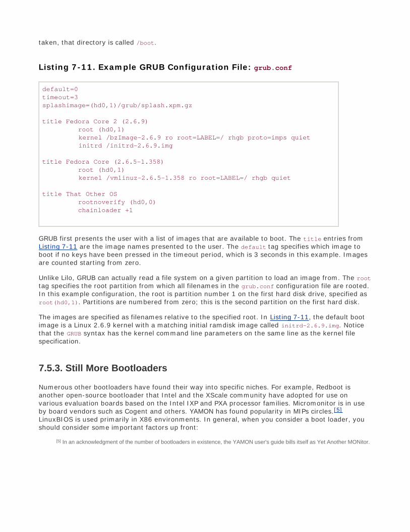
taken, that directory is called /boot.
Listing 7-11. Example GRUB Configuration File: grub.conf
default=0timeout=3splashimage=(hd0,1)/grub/splash.xpm.gz
title Fedora Core 2 (2.6.9) root (hd0,1) kernel /bzImage-2.6.9 ro root=LABEL=/ rhgb proto=imps quiet initrd /initrd-2.6.9.img
title Fedora Core (2.6.5-1.358) root (hd0,1) kernel /vmlinuz-2.6.5-1.358 ro root=LABEL=/ rhgb quiet
title That Other OS rootnoverify (hd0,0) chainloader +1
GRUB first presents the user with a list of images that are available to boot. The title entries fromListing 7-11 are the image names presented to the user. The default tag specifies which image toboot if no keys have been pressed in the timeout period, which is 3 seconds in this example. Imagesare counted starting from zero.
Unlike Lilo, GRUB can actually read a file system on a given partition to load an image from. The roottag specifies the root partition from which all filenames in the grub.conf configuration file are rooted.In this example configuration, the root is partition number 1 on the first hard disk drive, specified asroot(hd0,1). Partitions are numbered from zero; this is the second partition on the first hard disk.
The images are specified as filenames relative to the specified root. In Listing 7-11, the default bootimage is a Linux 2.6.9 kernel with a matching initial ramdisk image called initrd-2.6.9.img. Noticethat the GRUB syntax has the kernel command line parameters on the same line as the kernel filespecification.
7.5.3. Still More Bootloaders
Numerous other bootloaders have found their way into specific niches. For example, Redboot isanother open-source bootloader that Intel and the XScale community have adopted for use onvarious evaluation boards based on the Intel IXP and PXA processor families. Micromonitor is in useby board vendors such as Cogent and others. YAMON has found popularity in MIPs circles.[5]
LinuxBIOS is used primarily in X86 environments. In general, when you consider a boot loader, youshould consider some important factors up front:
[5] In an acknowledgment of the number of bootloaders in existence, the YAMON user's guide bills itself as Yet Another MONitor.

Does it support my chosen processor?
Has it been ported to a board similar to my own?
Does it support the features I need?
Does it support the hardware devices I intend to use?
Is there a large community of users where I might get support?
Are there any commercial vendors from which I can purchase support?
These are some of the questions you must answer when considering what bootloader to use in yourembedded project. Unless you are doing something on the "bleeding edge" of technology using abrand-new processor, you are likely to find that someone has already done the bulk of the hard workin porting a bootloader to your chosen platform. Use the resources at the end of this chapter to helpmake your final decisions.

7.6. Chapter Summary
The bootloader's role in an embedded system cannot be overstated. It is the first piece ofsoftware that takes control upon applying power.
This chapter examined the role of the bootloader and discovered the limited execution contextin which a bootloader must exist.
Das U-Boot has become a popular universal bootloader for many processor architectures. Itsupports a large number of processors, reference hardware platforms, and custom boards.
U-Boot is configured using a series of configuration variables in a board-specific header file.Appendix B, contains a list of all the standard U-Boot command sets supported in a recent U-Boot release.
Porting U-Boot to a new board based on a supported processor is relatively straightforward. Inthis chapter, we walked through the steps of a typical port to a board with similar support in U-Boot.
There is no substitute for detailed knowledge of your processor and hardware platform whenbootloader modification or porting must be accomplished.
We briefly introduced additional bootloaders in use today so you can make an informed choicefor your particular requirements.
7.6.1. Suggestions for Additional Reading
Application Note: Introduction to Synchronous DRAMMaxwell Technologieswww.maxwell.com/pdf/me/app_notes/Intro_to_SDRAM.pdf
Using LD, the GNU linkerFree Software Foundationwww.gnu.org/software/binutils/manual/ld-2.9.1/ld.html
The DENX U-Boot and Linux Guide (DLUG) for TQM8xxLWolfgang Denx et al., Denx Software Engineeringwww.denx.de/twiki/bin/view/DULG/Manual
RFC 793, "Trivial File Transfer Protocol"The Internet Engineering Task Forcewww.ietf.org/rfc/rfc793.txt
RFC 951, "Bootstrap Protocol"The Internet Engineering Task Force

www.ietf.org/rfc/rfc951.txt
RFC 1531, "Dynamic Host Control Protocol"The Internet Engineering Task Forcewww.ietf.org/rfc/rfc1531.txt
PowerPC 405GP Embedded Processor user's manualInternational Business Machines, Inc.
Programming Environments Manual for 32-bit Implementationsof the PowerPC ArchitectureFreescale Semiconductor, Inc.
Lilo Bootloaderwww.tldp.org/HOWTO/LILO.html
GRUB Bootloader www.gnu.org/software/grub/

Chapter 8. Device Driver BasicsIn this chapter
Device Driver Concepts page 190
Module Utilities page 199
Driver Methods page 205
Bringing It All Together page 209
Device Drivers and the GPL page 211
Chapter Summary page 211
One of the more challenging aspects of system design is partitioning functionality in a rationalmanner. The familiar device driver model found in UNIX and Linux provides a natural partitioning offunctionality between your application code and hardware or kernel devices. In this chapter, wedevelop an understanding of this model and the basics of Linux device driver architecture. Afterreading this chapter, you will have a solid foundation for continuing your study of device drivers usingone of the excellent texts listed at the end of this chapter.
This chapter begins by presenting Linux device driver concepts and the build system for drivers withinthe kernel source tree. We examine the Linux device driver architecture and present a simple workingexample driver. We introduce the user space utilities for loading and unloading kernel modules.[1] Wepresent a simple application to illustrate the interface between applications and device drivers. Weconclude this chapter with a discussion of device drivers and the GNU Public License.
[1] The terms module and device driver are used here interchangeably.

8.1. Device Driver Concepts
Many experienced embedded developers struggle at first with the concepts of device drivers in avirtual memory operating system. This is because many popular legacy real-time operating systemsdo not have a similar architecture. The introduction of virtual memory and kernel space versus userspace frequently introduces complexity that is not familiar to experienced embedded developers.
One of the fundamental purposes of a device driver is to isolate the user's programs from readyaccess to critical kernel data structures and hardware devices. Furthermore, a well-written devicedriver hides the complexity and variability of the hardware device from the user. For example, aprogram that wants to write data to the hard disk need not care if the disk drive uses 512-byte or1024-byte sectors. The user simply opens a file and issues a write command. The device driverhandles the details and isolates the user from the complexities and perils of hardware deviceprogramming. The device driver provides a consistent user interface to a large variety of hardwaredevices. It provides the basis for the familiar UNIX/Linux convention that everything must berepresented as a file.
8.1.1. Loadable Modules
Unlike some other operating systems, Linux has the capability to add and remove kernel componentsat runtime. Linux is structured as a monolithic kernel with a well-defined interface for adding andremoving device driver modules dynamically after boot time. This feature not only adds flexibility tothe user, but it has proven invaluable to the device driver development effort. Assuming that yourdevice driver is reasonably well behaved, you can insert and remove the device driver from a runningkernel at will during the development cycle instead of rebooting the kernel every time a changeoccurs.
Loadable modules have particular importance to embedded systems. Loadable modules enhance fieldupgrade capabilities; the module itself can be updated in a live system without the need for a reboot.Modules can be stored on media other than the root (boot) device, which can be space constrained.
Of course, device drivers can also be statically compiled into the kernel, and, for many drivers, this iscompletely appropriate. Consider, for example, a kernel configured to mount a root file system froma network-attached NFS server. In this scenario, you configure the network-related drivers (TCP/IPand the network interface card driver) to be compiled into the main kernel image so they areavailable during boot for mounting the remote root file system. You can use the initial ramdiskfunctionality as described in Chapter 6, "System Initialization," as an alternative to having thesedrivers compiled statically as part of the kernel proper. In this case, the necessary modules and ascript to load them would be included in the initial ramdisk image.
Loadable modules are installed after the kernel has booted. Startup scripts can load device drivermodules, and modules can also be "demand loaded" when needed. The kernel has the capability torequest a module when a service is requested that requires a particular module.
Terminology has never been standardized when discussing kernel modules. Many terms have been

and continue to be used interchangeably when discussing loadable kernel modules. Throughout thisand later chapters, the terms device driver, loadable kernel module (LKM), loadable module, andmodule are all used to describe a loadable kernel device driver module.
8.1.2. Device Driver Architecture
The basic Linux device driver model is familiar to UNIX/Linux system developers. Although the devicedriver model continues to evolve, some fundamental constructs have remained nearly constant overthe course of UNIX/Linux evolution. Device drivers are broadly classified into two basic categories:character devices and block devices. Character devices can be thought of as serial streams ofsequential data. Examples of character devices include serial ports and keyboards. Block devices arecharacterized by the capability to read and write blocks of data to and from random locations on anaddressable medium. Examples of block devices include hard drives and floppy disk drives.
8.1.3. Minimal Device Driver Example
Because Linux supports loadable device drivers, it is relatively easy to demonstrate a simple devicedriver skeleton. Listing 8-1 illustrates a loadable device driver module that contains the bareminimum structure to be loaded and unloaded by a running kernel.
Listing 8-1. Minimal Device Driver
/* Example Minimal Character Device Driver */#include <linux/module.h>
static int __init hello_init(void){ printk("Hello Example Init\n");
return 0;}
static void __exit hello_exit(void){ printk("Hello Example Exit\n");}
module_init(hello_init);module_exit(hello_exit);
MODULE_AUTHOR("Chris Hallinan");MODULE_DESCRIPTION("Hello World Example");

MODULE_LICENSE("GPL");
The skeletal driver in Listing 8-1 contains enough structure for the kernel to load and unload thedriver, and to invoke the initialization and exit routines. Let's look at how this is done because itillustrates some important high-level concepts that are useful for device driver development.
A device driver is a special kind of binary module. Unlike a stand-alone binary executable application,a device driver cannot be simply executed from a command prompt. The 2.6 kernel series requiresthat the binary be in a special "kernel object" format. When properly built, the device driver binarymodule contains a .ko suffix. The build steps and compiler options required to create the .ko moduleobject can be quite complex. Here we outline a set of steps to harness the power of the Linux kernelbuild system without requiring you to become an expert in it, which is beyond the scope of this book.
8.1.4. Module Build Infrastructure
A device driver must be compiled against the kernel on which it will execute. Although it is possible toload and execute kernel modules built against a different kernel version, it is risky to do so unlessyou are certain that the module does not rely on any features of your new kernel. The easiest way todo this is to build the module within the kernel's own source tree. This ensures that as the developerchanges the kernel configuration, his custom driver is automatically rebuilt with the correct kernelconfiguration. It is certainly possible to build your drivers outside of the kernel source tree. However,in this case, you are responsible for making sure that your device driver build configuration stays insync with the kernel you want to run your driver on. This typically includes compiler switches,location of kernel header files, and kernel configuration options.
For the example driver introduced in Listing 8-1, the following changes were made to the stock Linuxkernel source tree to enable building this example driver. We explain each step in detail.
1. Starting from the top-level Linux source directory, create a directory under .../drivers/charcalled examples.
2. Add a menu item to the kernel configuration to enable building examples and to specify built-inor loadable kernel module.
3. Add the new examples subdirectory to the .../drivers/char/Makefile conditional on the menuitem created in step 2.
4. Create a makefile for the new examples directory, and add the hello1.o module object to becompiled conditional on the menu item created in step 2.
5. Finally, create the driver hello1.c source file from Listing 8.1.
Adding the examples directory under the .../drivers/char subdirectory is self-explanatory. After thisdirectory is created, two files are created in this directory: the module source file itself from Listing 8-1 and the makefile for the examples directory. The makefile for examples is quite trivial. It will containthis single line:

obj-$(CONFIG_EXAMPLES) += hello1.o
Adding the menu item to the kernel configuration utility is a little more involved. Listing 8-2 containsa patch that, when applied to the .../drivers/char/Kconfig file from a recent Linux release, addsthe configuration menu item to enable our examples configuration option. For those readers notfamiliar with the diff/patch format, each line in Listing 8-1 preceded by a single plus (+) character isinserted in the file between the indicated lines (those without the leading + character).
Listing 8-2. Kconfig Patch for Examples
diff -u ~/base/linux-2.6.14/drivers/char/Kconfig./drivers/char/Kconfig--- ~/base/linux-2.6.14/drivers/char/Kconfig+++ ./drivers/char/Kconfig@@ -4,6 +4,12 @@
menu "Character devices"
+config EXAMPLES + tristate "Enable Examples" + default M + ---help--- + Enable compilation option for driver examples + config VT bool "Virtual terminal" if EMBEDDED select INPUT
When applied to Kconfig in the .../drivers/char subdirectory of a recent Linux kernel, this patchresults in a new kernel configuration option called CONFIG_EXAMPLES. As a reminder from ourdiscussion on building the Linux kernel in Chapter 4, "The Linux KernelA Different Perspective," theconfiguration utility is invoked as follows (this example assumes the ARM architecture):
$ make ARCH=ARM CROSS_COMPILE=xscale_be- gconfig
After the configuration utility is invoked using a command similar to the previous one, our new EnableExamples configuration option appears under the Character devices menu, as indicated in the patch.Because it is defined as type tristate, the kernel developer can choose from three choices:
(N) No. Do not compile examples.
(Y) Yes. Compile examples and link with final kernel image.
(M) Module. Compile examples as dynamically loadable module.
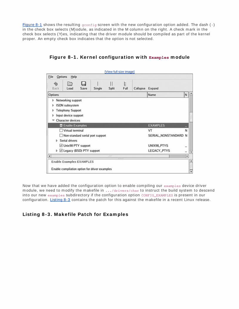
Figure 8-1 shows the resulting gconfig screen with the new configuration option added. The dash (-)in the check box selects (M)odule, as indicated in the M column on the right. A check mark in thecheck box selects (Y)es, indicating that the driver module should be compiled as part of the kernelproper. An empty check box indicates that the option is not selected.
Figure 8-1. Kernel configuration with Examples module
[View full size image]
Now that we have added the configuration option to enable compiling our examples device drivermodule, we need to modify the makefile in .../drivers/char to instruct the build system to descendinto our new examples subdirectory if the configuration option CONFIG_EXAMPLES is present in ourconfiguration. Listing 8-3 contains the patch for this against the makefile in a recent Linux release.
Listing 8-3. Makefile Patch for Examples

diff -u ~/base/linux-2.6.14/drivers/char/Makefile./drivers/char/Makefile--- ~/base/linux-2.6.14/drivers/char/Makefile+++ ./drivers/char/Makefile@@ -88,6 +88,7 @@ obj-$(CONFIG_DRM) += drm/ obj-$(CONFIG_PCMCIA) += pcmcia/ obj-$(CONFIG_IPMI_HANDLER) += ipmi/+obj-$(CONFIG_EXAMPLES) += examples/
obj-$(CONFIG_HANGCHECK_TIMER) += hangcheck-timer.o
The patch in Listing 8-3 adds the single line (preceded by the + character) to the makefile found in.../drivers/char. The additional lines of context are there so that the patch utility can determinewhere to insert the new line. Our new examples directory was added to the end of the list ofdirectories already being searched in this makefile, which seemed like a logical place to put it. Otherthan for consistency and readability, the location is irrelevant.
Having completed the steps in this section, the infrastructure is now in place to build the exampledevice driver. The beauty of this approach is that the driver is built automatically whenever a kernelbuild is invoked. As long as the configuration option defined in Listing 8-3 is selected (either M or Y),the driver module is included in the build.
Building for an arbitrary ARM system, the command line for building modules might look like this:
$ make ARCH=arm CROSS_COMPILE=xscale_be- modules
Listing 8-4 shows the build output after a typical editing session on the module (all other moduleshave already been built in this kernel source tree.)
Listing 8-4. Module Build Output
$ make ARCH=arm CROSS_COMPILE=xscale_be- modules CHK include/linux/version.hmake[1]: 'arch/arm/kernel/asm-offsets.s' is up to date.make[1]: 'include/asm-arm/mach-types.h' is up to date. CC [M] drivers/char/examples/hello1.o Building modules, stage 2. MODPOST LD [M] drivers/char/examples/hello1.ko
8.1.5. Installing Your Device Driver
Now that this driver is built, we can load and unload it on a running kernel to observe its behavior.Before we can load the module, we need to copy it to an appropriate location on our target system.

Although we could put it anywhere we want, a convention is in place for kernel modules and wherethey are populated on a running Linux system. As with module compilation, it is easiest to let thekernel build system do that for us. The makefile target modules_install automatically places modulesin the system in a logical layout. You simply need to supply the desired location as a prefix to thedefault path.
In a standard Linux workstation installation, you might already know that the device driver moduleslive in /lib/modules/<kernel-version>/... ordered in a manner similar to the device driver directoryhierarchy in the Linux kernel tree.[2] The <kernel-version> string is produced by executing thecommand uname -r on your target Linux system. If you do not provide an installation prefix to thekernel build system, by default, your modules are installed in your own workstation's/lib/modules/... directory. This is probably not what you had intended. You can point to atemporary location in your home directory and manually copy the modules to your target's filesystem. Alternatively, if your target embedded system uses NFS root mount to a directory on yourlocal development workstation, you can install the modules directly to the target file system. Thefollowing example assumes the latter.
[2] This path is used by Red Hat and Fedora distributions, and is also required by the File System Hierarchy Standard referenced
at the end of this chapter. Other distributions might use different locations in the file system for kernel modules.
$ make ARCH=arm CROSS_COMPILE=xscale_be- \ INSTALL_MOD_PATH=/home/chris/sandbox/coyote-target \ modules_install
This places all your modules in the directory coyote-target, which on this example system isexported via NFS and mounted as root on the target system.[3]
[3] Hosting a target board and NFS root mount are covered in detail in Chapter 12, "Embedded Development Environment".
8.1.6. Loading Your Module
Having completed all the steps necessary, we are now in a position to load and test the device drivermodule. Listing 8-5 shows the output resulting from loading and subsequently unloading the devicedriver on the embedded system.
Listing 8-5. Loading and Unloading a Module
$ modprobe hello1 <<< Load the driverHello Example Init$ modprobe -r hello1 <<< Unload the driverHello Example Exit$
You should be able to correlate the output with our device driver source code found in Listing 8-1.The module does no work other than printing messages to the kernel log system via printk(), whichwe see on our console.[4] When the module is loaded, the module-initialization function is called. Wespecify the initialization function that will be executed on module insertion using the module_init()

macro. We declared it as follows:
[4] If you don't see the messages on the console, either disable your syslogd logger or lower the console loglevel. We describe
how to do this in Chapter 14, "Kernel Debugging Techniques".
module_init(hello_init);
In our initialization function, we simply print the obligatory hello message and return. In a real devicedriver, this is where you would perform any initial resource allocation and hardware deviceinitialization. In a similar fashion, when we unload the module (using the modprobe -r command), ourmodule exit routine is called. As shown in Listing 8-1, the exit routine is specified using themodule_exit() macro.
That's all there is to a skeletal device driver capable of live insertion in an actual kernel. In thesections to follow, we introduce additional functionality to our loadable device driver module thatillustrates how a user space program would interact with a device driver module.

8.2. Module Utilities
We had a brief introduction to module utilities in Listing 8-5. There we used the module utilitymodprobe to insert and remove a device driver module from a Linux kernel. A number of small utilitiesare used to manage device driver modules. This section introduces them. You are encouraged torefer to the man page for each utility, for complete details. In fact, those interested in a greaterknowledge of Linux loadable modules should consult the source code for these utilities. Section 8.6.1,"Suggestions for Additional Reading" at the end of this chapter contains a reference for where theycan be found.
8.2.1. insmod
The insmod utility is the simplest way to insert a module into a running kernel. You supply a completepathname, and insmod does the work. For example:
$ insmod /lib/modules/2.6.14/kernel/drivers/char/examples/hello1.ko
This loads the module hello1.ko into the kernel. The output would be the same as shown in Listing8-5namely, the Hello message. The insmod utility is a simple program that does not require oraccept any options. It requires a full pathname because it has no logic for searching for the module.Most often, you will use modprobe, described shortly, because it has many more features andcapabilities.
8.2.2. Module Parameters
Many device driver modules can accept parameters to modify their behavior. Examples includeenabling debug mode, setting verbose reporting, or specifying module-specific options. The insmodutility accepts parameters (also called options in some contexts) by specifying them after the modulename. Listing 8-6 shows our modified hello1.c example, adding a single module parameter to enabledebug mode.
Listing 8-6. Example Driver with Parameter
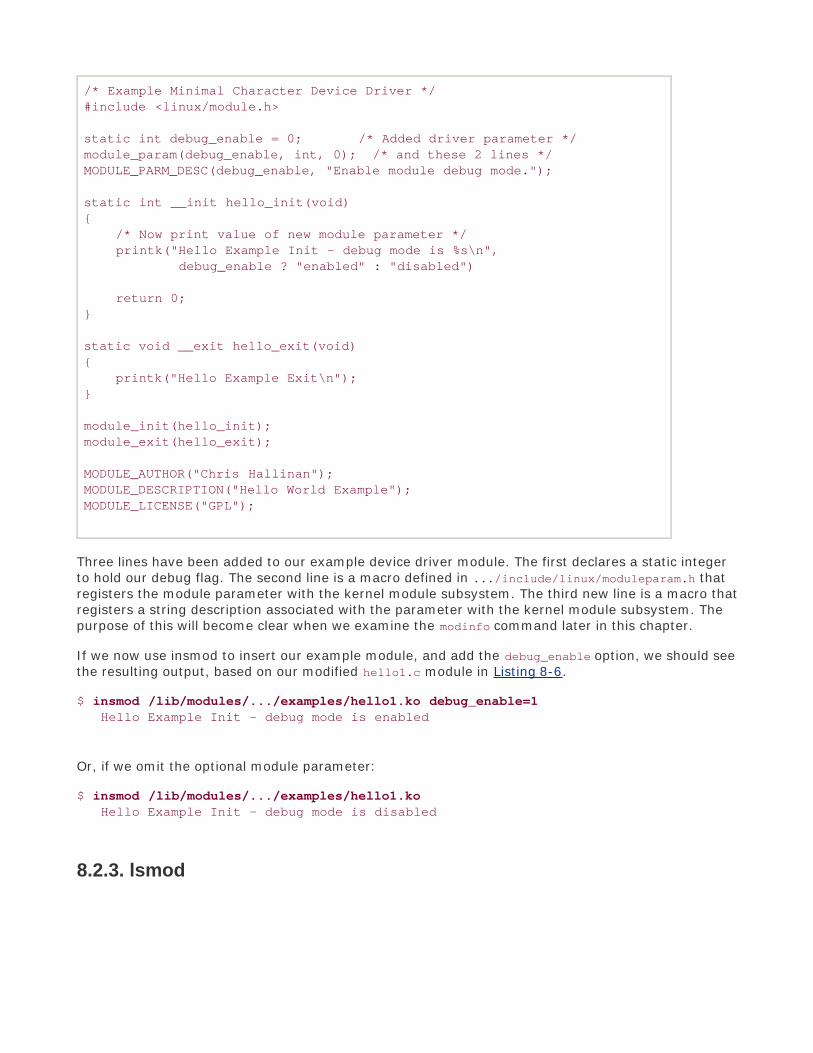
/* Example Minimal Character Device Driver */#include <linux/module.h>
static int debug_enable = 0; /* Added driver parameter */module_param(debug_enable, int, 0); /* and these 2 lines */MODULE_PARM_DESC(debug_enable, "Enable module debug mode.");
static int __init hello_init(void){ /* Now print value of new module parameter */ printk("Hello Example Init - debug mode is %s\n", debug_enable ? "enabled" : "disabled")
return 0;}
static void __exit hello_exit(void){ printk("Hello Example Exit\n");}
module_init(hello_init);module_exit(hello_exit);
MODULE_AUTHOR("Chris Hallinan");MODULE_DESCRIPTION("Hello World Example");MODULE_LICENSE("GPL");
Three lines have been added to our example device driver module. The first declares a static integerto hold our debug flag. The second line is a macro defined in .../include/linux/moduleparam.h thatregisters the module parameter with the kernel module subsystem. The third new line is a macro thatregisters a string description associated with the parameter with the kernel module subsystem. Thepurpose of this will become clear when we examine the modinfo command later in this chapter.
If we now use insmod to insert our example module, and add the debug_enable option, we should seethe resulting output, based on our modified hello1.c module in Listing 8-6.
$ insmod /lib/modules/.../examples/hello1.ko debug_enable=1 Hello Example Init - debug mode is enabled
Or, if we omit the optional module parameter:
$ insmod /lib/modules/.../examples/hello1.ko Hello Example Init - debug mode is disabled
8.2.3. lsmod

The lsmod utility is also quite trivial. It simply displays a formatted list of the modules that areinserted into the kernel. Recent versions take no parameters and simply format the output of/proc/modules.[5] Listing 8-7 is an example of the output from lsmod.
[5] /proc/modules is part of the proc file system, which is introduced in Chapter 9, "File Systems".
Listing 8-7. lsmod Example Output Format
$ lsmodModule Size Used byext3 121096 0jbd 49656 1 ext3loop 12712 0hello1 1412 0$
Notice the rightmost column labeled Used by. This column indicates that the device driver module isin use and shows the dependency chain. In this example, the jbd module (journaling routines forjournaling file systems) is being used by the ext3 module, the default journaling file system for manypopular Linux desktop distributions. This means that the ext3 device driver depends on the presenceof jbd.
8.2.4. modprobe
This is where the cleverness of modprobe comes into play. In Listing 8-7, we see the relationshipbetween the ext3 and jbd modules. The ext3 module depends on the jbd module. The modprobeutility can discover this relationship and load the dependent modules in the proper order. Thefollowing command loads both the jbd.ko and ext3.ko driver modules:
$ modprobe ext3
The modprobe utility has several command line options that control its behavior. As we saw earlier,modprobe can be used to remove modules, including the modules upon which a given moduledepends. Here is an example of module removal that removes both jbd.ko and ext3.ko:
$ modprobe -r ext3
The modprobe utility is driven by a configuration file called modprobe.conf. This enables a systemdeveloper to associate devices with device drivers. For a simple embedded system, modprobe.confmight be empty or might contain very few lines. The modprobe utility is compiled with a set of defaultrules that establish the defaults in the absence of a valid modprobe.conf. Invoking modprobe withonly the -c option displays the set of default rules used by modprobe.
Listing 8-8 represents a typical modprobe.conf, which might be found on a system containing twoEthernet interfaces; one is a wireless adapter based on the Prism2 chipset, and the other is a typical

PCI Ethernet card. This system also contains a sound subsystem based on an integrated Intel soundchipset.
Listing 8-8. Typical modprobe.conf File
$ cat /etc/modprobe.confalias eth1 orinoci_pcioptions eth1 orinoco_debug=9alias eth0 e100alias snd-card-0 snd-intel8x0options snd-card-0 index=0$
When the kernel boots and discovers the wireless chipset, this configuration file instructs modprobeto load the orinoco_pci device driver, bound to kernel device eth1, and pass the optional moduleparameter orinoco_debug=9 to the device driver. The same action is taken upon discovery of thesound card hardware. Notice the optional parameters associated with the sound driver snd-intel8x0.
8.2.5. depmod
How does modprobe know about the dependencies of a given module? The depmod utility plays a keyrole in this process. When modprobe is executed, it searches for a file called modules.dep in the samelocation where the modules are installed. The depmod utility creates this module-dependency file.
This file contains a list of all the modules that the kernel build system is configured for, along withdependency information for each. It is a simple file format: Each device driver module occupies oneline in the file. If the module has dependencies, they are listed in order following the module name.For example, from Listing 8-7, we saw that the ext3 module had a dependency on the jbd module.The dependency line in modules.dep would look like this:
ext3.ko: jbd.ko
In actual practice, each module name is preceded by its absolute path in the file system, to avoidambiguity. We have omitted the path information for readability. A more complicated dependencychain, such as sound drivers, might look like this:
snd-intel8x0.ko: snd-ac97-codec.ko snd-pcm.ko snd-timer.ko \ snd.ko soundcore.ko snd-page-alloc.ko
Again, we have removed the leading path components for readability. Each module filename in themodules.dep file is an absolute filename, with complete path information, and exists on a single line.The previous example has been truncated to two lines, to fit in the space on this page.
Normally, depmod is run automatically during a kernel build. However, in a cross-developmentenvironment, you must have a cross-version of depmod that knows how to read the modules that

are compiled in the native format of your target architecture. Alternatively, most embeddeddistributions have a method and init script entries to run depmod on each boot, to guarantee thatthe module dependencies are kept up-to-date.
8.2.6. rmmod
This utility is also quite trivial. It simply removes a module from a running kernel. Pass it the modulename as a parameter. There is no need to include a pathname or file extension. For example:
$ rmmod hello1 Hello Example Exit
The only interesting point to understand here is that when you use rmmod, it executes the module's*_exit() function, as shown in the previous example, from our hello1.c example of Listings 8-1 and8-6.
It should be noted that, unlike modprobe, rmmod does not remove dependent modules. Usemodprobe -r for this.
8.2.7. modinfo
You might have noticed the last three lines of the skeletal driver in Listing 8-1, and later in Listing 8-6. These macros are there to place tags in the binary module to facilitate their administration andmanagement. Listing 8-9 is the result of modinfo executed on our hello1.ko module.
Listing 8-9. modinfo Output
$ modinfo hello1filename: /lib/modules/.../char/examples/hello1.koauthor: Chris Hallinandescription: Hello World Examplelicense: GPLvermagic: 2.6.14 ARMv5 gcc-3.3depends:parm: debug_enable:Enable module debug mode. (int)$
The first field is obvious: It is the full filename of the device driver module. For readability in thislisting, we have truncated the path again. The next lines are a direct result of the descriptive macrosfound at the end of Listing 8-6namely, the filename, author, and license information. These aresimply tags for use by the module utilities and do not affect the behavior of the device driver itself.You can learn more about modinfo from its man page and the modinfo source itself.
One very useful feature of modinfo is to learn what parameters the module supports. From Listing 8-

9, you can see that this module supports just one parameter. This was the one we added in Listing 8-6, debug_enable. The listing gives the name, type (in this case, an int), and descriptive text field weentered with the MODULE_PARM_DESC() macro. This can be very handy, especially for modules in whichyou might not have easy access to the source code.

8.3. Driver Methods
We've covered much ground in our short treatment of module utilities. In the remaining sections ofthis chapter, we describe the basic mechanism for communicating with a device driver from a userspace program (your application code).
We have introduced the two fundamental methods responsible for one-time initialization and exitprocessing of the module. Recall from Listing 8-1 that these are module_init() and module_exit().We discovered that these routines are invoked at the time the module is inserted into or removedfrom a running kernel. Now we need some methods to interface with our device driver from ourapplication program. After all, two of the more important reasons we use device drivers are to isolatethe user from the perils of writing code in kernel space and to present a unified method tocommunicate with hardware or kernel-level devices.
8.3.1. Driver File System Operations
After the device driver is loaded into a live kernel, the first action we must take is to prepare thedriver for subsequent operations. The open() method is used for this purpose. After the driver hasbeen opened, we need routines for reading and writing to the driver. A release() routine is providedto clean up after operations when complete (basically, a close call). Finally, a special system call isprovided for nonstandard communication to the driver. This is called ioctl(). Listing 8-10 adds thisinfrastructure to our example device driver.
Listing 8-10. Adding File System Ops to Hello.c
#include <linux/module.h>#include <linux/fs.h>
#define HELLO_MAJOR 234
static int debug_enable = 0;module_param(debug_enable, int, 0);MODULE_PARM_DESC(debug_enable, "Enable module debug mode.");
struct file_operations hello_fops;
static int hello_open(struct inode *inode, struct file *file){

printk("hello_open: successful\n"); return 0;}
static int hello_release(struct inode *inode, struct file *file){
printk("hello_release: successful\n"); return 0;}
static ssize_t hello_read(struct file *file, char *buf, size_t count, loff_t *ptr){
printk("hello_read: returning zero bytes\n"); return 0;}
static ssize_t hello_write(struct file *file, const char *buf, size_t count, loff_t * ppos){
printk("hello_read: accepting zero bytes\n"); return 0;}
static int hello_ioctl(struct inode *inode, struct file *file, unsigned int cmd, unsigned long arg){
printk("hello_ioctl: cmd=%ld, arg=%ld\n", cmd, arg); return 0;}
static int __init hello_init(void){ int ret; printk("Hello Example Init - debug mode is %s\n", debug_enable ? "enabled" : "disabled"); ret = register_chrdev(HELLO_MAJOR, "hello1", &hello_fops); if (ret < 0) { printk("Error registering hello device\n"); goto hello_fail1; } printk("Hello: registered module successfully!\n");

/* Init processing here... */
return 0;
hello_fail1: return ret;}
static void __exit hello_exit(void){ printk("Hello Example Exit\n");}
struct file_operations hello_fops = { owner: THIS_MODULE, read: hello_read, write: hello_write, ioctl: hello_ioctl, open: hello_open, release: hello_release,};
module_init(hello_init);module_exit(hello_exit);
MODULE_AUTHOR("Chris Hallinan");MODULE_DESCRIPTION("Hello World Example");MODULE_LICENSE("GPL");
This expanded device driver example includes many new lines. From the top, we've had to add a newkernel header file to get the definitions for the file system operations. We've also defined a majornumber for our device driver. (Note to device driver authors: This is not the proper way to allocate anumber for our device driver. (Note to device driver authors: This is not the proper way to allocate adevice driver major number. Refer to the Linux kernel documentation(.../Documentation/devices.txt) or one of the excellent texts on device drivers for guidance on theallocation of major device numbers. For this simple example, we simply choose one that we knowisn't in use on our system.)
Next we see definitions for four new functions, our open, close, read, and write methods. In keepingwith good coding practices, we've adopted a consistent naming scheme that will not collide with anyother subsystems in the kernel. Our new methods are called hello_open(), hello_release(),hello_read(), and hello_write(), respectively. For purposes of this simple exercise, they are do-nothing functions that simply print a message to the kernel log subsystem.
Notice that we've also added a new function call to our hello_init() routine. This line registers our

device driver with the kernel. With that registration call, we pass a structure containing pointers tothe required methods. The kernel uses this structure, of type struct file_operations, to bind ourspecific device functions with the appropriate requests from the file system. When an applicationopens a device represented by our device driver and requests a read() operation, the file systemassociates that generic read() request with our module's hello_read() function. The followingsections examine this process in detail.
8.3.2. Device Nodes and mknod
To understand how an application binds its requests to a specific device represented by our devicedriver, we must understand the concept of a device node. A device node is a special file type in Linuxthat represents a device. Virtually all Linux distributions keep device nodes in a common location(specified by the Filesystem Hierarchy Standard [6]), in a directory called /dev. A dedicated utility isused to create a device node on a file system. This utility is called mknod.
[6] Reference to this standard is found in the "Suggestions for Additional Reading," at the end of this chapter.
An example of node creation is the best way to illustrate its functionality and the information itconveys. In keeping with our simple device driver example, let's create the proper device node toexercise it:
$ mknod /dev/hello1 c 234 0
After executing this command on our target embedded system, we end up with a new file called/dev/hello1 that represents our device driver module. If we list this file to the console, it looks likethis:
$ ls -l /dev/hello1crw-r--r-- 1 root root 234, 0 Jul 14 2005 /dev/hello1
The parameters we passed to mknod include the name, type, and major and minor numbers for ourdevice driver. The name we chose, of course, was hello1. Because we are demonstrating the use ofa character driver, we use c to indicate that. The major number is 234, the number we chose for thisexample, and the minor number is 0.
By itself, the device node is just another file on our file system. However, because of its special statusas a device node, we use it to bind to an installed device driver. If an application process issues anopen() system call with our device node as the path parameter, the kernel searches for a valid devicedriver registered with a major number that matches the device nodein our case, 234. This is themechanism by which the kernel associates our particular device to the device node.
As most C programmers know, the open() system call, or any of its variants, returns a reference (filedescriptor) that our applications use to issue subsequent file system operations, such as read, write,and close. This reference is then passed to the various file system operations, such as read, write, ortheir variants.
For those curious about the purpose of the minor number, it is a mechanism for handling multipledevices or subdevices with a single device driver. It is not used by the operating system; it is simplypassed to the device driver. The device driver can use the minor number in any way it sees fit. As an

example, with a multiport serial card, the major number would specify the driver. The minor numbermight specify one of the multiple ports handled by the same driver on the multiport card. Interestedreaders are encouraged to consult one of the excellent texts on device drivers for further details.

8.4. Bringing It All Together
Now that we have a skeletal device driver, we can load it and exercise it. Listing 8-11 is a simple userspace application that exercises our device driver. We've already seen how to load the driver. Simplycompile it and issue the make modules_install command to place it on your file system, as previouslydescribed.
Listing 8-11. Exercising Our Device Driver
#include <stdio.h>#include <stdlib.h>#include <sys/types.h>#include <sys/stat.h>#include <fcntl.h>#include <unistd.h>
int main(int argc, char **argv){ /* Our file descriptor */ int fd; int rc = 0; char *rd_buf[16];
printf("%s: entered\n", argv[0]);
/* Open the device */ fd = open("/dev/hello1", O_RDWR); if ( fd == -1 ) { perror("open failed"); rc = fd; exit(-1); } printf("%s: open: successful\n", argv[0]); /* Issue a read */ rc = read(fd, rd_buf, 0); if ( rc == -1 ) { perror("read failed"); close(fd); exit(-1); } printf("%s: read: returning %d bytes!\n", argv[0], rc);

close(fd); return 0;}
This simple file, compiled on an ARM XScale system, demonstrates the binding of application todevice driver, through the device node. Like the device driver, it doesn't do any useful work, but itdoes demonstrate the concepts as it exercises some of the methods we introduced in the devicedriver of Listing 8-10.
First we issue an open() system call [7] on our device node created earlier. If the open succeeds, weindicate that with a message to the console. Next we issue a read() command and again print amessage to the console on success. Notice that a read of 0 bytes is perfectly acceptable as far as thekernel is concerned and, in actual practice, indicates an end-of-file or out-of-data condition. Yourdevice driver defines that special condition. When complete, we simply close the file and exit. Listing8-12 captures the output of running this example application on an ARM XScale target:
[7] Actually, the open() call is a C library wrapper function around the Linux sys_open() system call.
Listing 8-12. Using the Example Driver
$ modprobe hello1Hello Example Init - debug mode is disabledHello: registered module successfully!$ ./use-hello./use-hello: entered./use-hello: open: successful./use-hello: read: returning zero bytes!$

8.5. Device Drivers and the GPL
Much discussion and debate surrounds the issue of device drivers and how the terms of the GNUPublic License apply to device drivers. The first test is well understood: If your device driver (or anysoftware, for that matter) is based, even in part, on existing GPL software, it is called a derived work.For example, if you start with a current Linux device driver and modify it to suit your needs, this iscertainly considered a derived work, and you are obligated to license this modified device driverunder the terms of the GPL, observing all its requirements.
This is where the debate comes in. First, the disclaimer. This is not a legal opinion, and the author isnot a lawyer. Some of these concepts have not been tested in court as of this writing. The prevailingopinion of the legal and open source communities is that if a work can be proven [8] to beindependently derived, and a given device driver does not assume "intimate knowledge" of the Linuxkernel, the developers are free to license it in any way they see fit. If modifications are made to thekernel to accommodate a special need of the driver, it is considered a derived work and, therefore, issubject to the GPL.
[8] This practice is not unique to open source. Copyright and patent infringement is an ongoing concern for all developers.
A large and growing body of information exists in the open source community regarding these issues.It seems likely that, at some point in the future, these concepts will be tested in a court of law andprecedent will be established. How long that might take is anyone's guess. If you are interested ingaining a better understanding of the legal issues surrounding Linux and open source, you mightenjoy www.open-bar.org.

8.6. Chapter Summary
This chapter presented a high-level overview of device driver basics and how they fit into thearchitecture of a Linux system. Armed with the basics, readers new to device drivers can jump intoone of the excellent texts devoted to device driver writers. Consult Section 8.6.1 for references.
Device drivers enforce a rational separation between unprivileged user applications and criticalkernel resources such as hardware and other devices, and present a well-known unifiedinterface to applications.
The minimum infrastructure to load a device driver is only a few lines of code. We presentedthis minimum infrastructure and built on the concepts to a simple shell of a driver module.
Device drivers configured as loadable modules can be inserted into and removed from a runningkernel after kernel boot.
Module utilities are used to manage the insertion, removal, and listing of device driver modules.We covered the details of the module utilities used for these functions.
Device nodes on your file system provide the glue between your userspace application and thedevice driver.
Driver methods implement the familiar open, read, write, and close functionality commonlyfound in UNIX/Linux device drivers. This mechanism was explained by example, including asimple user application to exercise these driver methods.
We concluded this chapter with an introduction to the relationship between kernel device driversand the Open Source GNU Public License.
8.6.1. Suggestions for Additional Reading
Linux Device Drivers, 3rd EditionAlessandro Rubini and Jonathan CorbetO'Reilly Publishing, 2005
Filesystem Hierarchy StandardEdited by Rusty Russel, Daniel Quinlan, and Christopher YeohThe File Systems Hierarchy Standards Groupwww.pathname.com/fhs/
Rusty's Linux Kernel PageModule Utilities for 2.6Rusty Russellhttp://kernel.org/pub/linux/kernel/people/rusty/


Chapter 9. File SystemsIn this chapter
Linux File System Concepts page 214
ext2 page 216
ext3 page 221
ReiserFS page 224
JFFS2 page 225
cramfs page 228
Network File System page 230
Pseudo File Systems page 234
Other File Systems page 240
Building a Simple File System page 242
Chapter Summary page 243
Perhaps one of the most important decisions an embedded developer makes is which file system(s)to deploy. Some file systems optimize for performance, whereas others optimize for size. Still othersoptimize for data recovery after device or power failure. This chapter introduces the major filesystems in use on Linux systems and examines the characteristics of each as they apply toembedded designs. It is not the intent of this chapter to examine the internal technical details of eachfile system. Instead, this chapter examines the operational characteristics and development issuesrelated to each file system presented. References in Section 9.11.1, "Suggestions for AdditionalReading," are provided at the end of the chapter for the interested reader.
Starting with the most popular file system in use on earlier Linux desktop distributions, we introduceconcepts using the Second Extended File System (ext2) to lay some foundation for further discussion.Next we look at its successor, the Third Extended File System (ext3), which is the default file systemfor many popular desktop Linux distributions being shipped today.
After introducing some fundamentals, we examine a variety of specialized file systems, includingthose optimized for data recovery and for storage space, and those designed for use on Flashmemory devices. The Network File System (NFS) is presented, followed by a discussion of the moreimportant Pseudo File Systems, including the proc file system and sysfs.

9.1. Linux File System Concepts
Before delving into the details of the individual file systems, let's look at the big picture of how data isstored on a Linux system. In our study of device drivers in Chapter 8, "Device Driver Basics," welooked at the structure of a character device. In general, character devices store and retrieve data inserial streams. The most basic example of a character device is a serial port or magnetic tape drive.In contrast, block devices store and retrieve data in equal-sized chucks of data at a time. Forexample, a typical IDE hard disk controller can transfer 512 bytes of data at a time to and from aspecific, addressable location on the physical media. File systems are based on block devices.
9.1.1. Partitions
Before we begin our discussion of file systems, we start by introducing partitions, the logical divisionof a physical device upon which a file system exists. At the highest level, data is stored on physicaldevices in partitions. A partition is a logical division of the physical medium (hard disk, Flashmemory) whose data is organized following the specifications of a given partition type. A physicaldevice can have a single partition covering all its available space, or it can be divided into multiplepartitions to suit a particular task. A partition can be thought of as a logical disk onto which acomplete file system can be written.
Figure 9-1 shows the relationship between partitions and file systems.
Figure 9-1. Partitions and file systems

Linux uses a utility called fdisk to manipulate partitions on block devices. A recent fdisk utility foundon many Linux distributions has knowledge of more than 90 different partition types. In practice, onlya few are commonly used on Linux systems. Some common partition types include Linux, FAT32, andLinux Swap.
Listing 9-1 displays the output of the fdisk utility targeting a CompactFlash device connected to aUSB port. On this particular target system, the USB subsystem assigned the CompactFlash physicaldevice to the device node /dev/sdb.
Listing 9-1. Displaying Partition Information Using fdisk
# fdisk /dev/sdbCommand (m for help): pDisk /dev/sdb: 49 MB, 49349120 bytes4 heads, 32 sectors/track, 753 cylindersUnits = cylinders of 128 * 512 = 65536 bytes
Device Boot Start End Blocks Id System/dev/sdb1 * 1 180 11504 83 Linux/dev/sdb2 181 360 11520 83 Linux/dev/sdb3 361 540 11520 83 Linux/dev/sdb4 541 753 13632 83 Linux
For this discussion, we have created four partitions on the device using the fdisk utility. One of themis marked bootable, as indicated by the asterisk in the column labeled Boot. This is simply the settingof a flag in the data structure that represents the partition table on the device. As you can see fromthe listing, the logical unit of storage used by fdisk is a cylinder.[1] On this device, a cylinder contains64KB. On the other hand, Linux represents the smallest unit of storage as a logical block. You candeduce from this listing that a block is a unit of 1024 bytes.
[1] The term cylinder was borrowed from the unit of storage on a rotational media. It consists of the data under a group of heads
on a given sector of a disk device. Here it is used for compatibility purposes with the existing file system utilities.
After the CompactFlash has been partitioned in this manner, each device representing a partition canbe formatted with a file system of your choice. When a partition is formatted with a given file systemtype, Linux can mount the corresponding file system from that partition.

9.2. ext2
Building on the example of Listing 9-1, we need to format the partitions created with fdisk. To do so,we use the Linux mke2fs utility. mke2fs is similar to the familiar DOS format command. This utilitymakes a file system of type ext2 on the specified partition. mke2fs is specific to the ext2 file system;other file systems have their own versions of these utilities. Listing 9-2 captures the output of thisprocess.
Listing 9-2. Formatting a Partition Using mke2fs
# mke2fs /dev/sdb1 -L CFlash_Boot_Volmke2fs 1.37 (21-Mar-2005)Filesystem label=CFlash_Boot_VolOS type: LinuxBlock size=1024 (log=0)Fragment size=1024 (log=0)2880 inodes, 11504 blocks575 blocks (5.00%) reserved for the super userFirst data block=1Maximum filesystem blocks=117964802 block groups8192 blocks per group, 8192 fragments per group1440 inodes per groupSuperblock backups stored on blocks: 8193
Writing inode tables: doneWriting superblocks and filesystem accounting information: done
This filesystem will be automatically checked every 39 mounts or180 days, whichever comes first. Use tune2fs -c or -i to override.#
Listing 9-2 contains a great deal of detail relating to the ext2 file system and provides an excellentway to begin to understand its operational characteristics. Note that this partition was formatted astype ext2 with a volume label of CFlash_Boot_Vol. It was created on a Linux partition (OS Type:) witha block size of 1024 bytes. Space was allocated for 2,880 inodes, occupying 11,504 blocks. An inodeis the fundamental data structure representing a single file. For more detailed information about theinternal structure of the ext2 file system, the reader is directed to Section 9.11.1 at the end of thischapter.
Looking at the output of mke2fs in Listing 9-2, we can ascertain certain characteristics of how the

storage device is organized. We already know that the block size is 1024 bytes. If necessary for yourparticular application, mke2fs can be instructed to format an ext2 file system with different blocksizes. Current implementations allow block sizes of 1,024, 2,048, and 4,096 blocks.
Block size is always a compromise for best performance. On one hand, large block sizes waste morespace on disks with many files because each file must fit into an integral number of blocks. Anyleftover fragment above block_size * n must occupy another full block, even if only 1 byte. On theother hand, very small block sizes increase the file system overhead of managing the metadata thatdescribes the block-to-file mapping. Benchmark testing on your particular hardware implementationis the only way to be sure you have selected an optimum block size.
9.2.1. Mounting a File System
After a file system has been created, we can mount that file system on a running Linux system,provided that we have access to the hardware device and that the kernel has been compiled withsupport for our particular file system type, either as a compiled-in module or a dynamically loadablemodule. The following command mounts the previously created ext2 file system on a mount pointthat we specify:
# mount /dev/sdb1 /mnt/flash
This example assumes that we have a directory created on our target Linux machine called/mnt/flash. This is called the mount point because we are installing (mounting) the file systemrooted at this point in our file system hierarchy. We are mounting the Flash device described earlierthat the kernel assigned to the device /dev/sdb1. On a typical Linux desktop (development) machine,we need to have root privileges to execute this command.[2] The mount point is any place on yourfile system that you decide, which becomes the top level (root) of your newly mounted device. In theprevious example, to reference any files on your Flash device, you must prefix the path with/mnt/flash.
[2] File systems can be made mountable by nonroot users, as with cdrom.
The mount command is a powerful command, with many options. Many of the options that mountaccepts depend on the target file system type of the mount operation. Most of the time, mount candetermine the type of file system on a properly formatted file system known to the kernel. Weprovide additional usage examples for the mount command as we proceed through this chapter.
Listing 9-3 displays the directory contents of a Flash device configured for an arbitrary embeddedsystem.
Listing 9-3. Flash Device Listing

$ ls -l /mnt/flashtotal 24drwxr-xr-x 2 root root 1024 Jul 18 20:18 bindrwxr-xr-x 2 root root 1024 Jul 18 20:18 bootdrwxr-xr-x 2 root root 1024 Jul 18 20:18 devdrwxr-xr-x 2 root root 1024 Jul 18 20:18 etcdrwxr-xr-x 2 root root 1024 Jul 18 20:18 homedrwxr-xr-x 2 root root 1024 Jul 18 20:18 libdrwx------ 2 root root 12288 Jul 17 13:02 lost+founddrwxr-xr-x 2 root root 1024 Jul 18 20:18 procdrwxr-xr-x 2 root root 1024 Jul 18 20:18 rootdrwxr-xr-x 2 root root 1024 Jul 18 20:18 sbindrwxr-xr-x 2 root root 1024 Jul 18 20:18 tmpdrwxr-xr-x 2 root root 1024 Jul 18 20:18 usrdrwxr-xr-x 2 root root 1024 Jul 18 20:18 var$
Listing 9-3 is an example of what an embedded systems root file system might look like at the top(root) level. Chapter 6, "System Initialization," provides guidance and examples for how to determinethe contents of the root file system.
9.2.2. Checking File System Integrity
The e2fsck command is used to check the integrity of an ext2 file system. A file system can becomecorrupted for several reasons, but by far the most common reason is an unexpected power failure orintentional power-down without first closing all open files and unmounting the file systems. Linuxdistributions perform these operations during the shutdown sequence (assuming an orderly shutdownof the system). However, when we are dealing with embedded systems, unexpected power-downsare common, and we need to provide some defensive measures against these cases. e2fsck is ourfirst line of defense for unexpected power-down using the ext2 file system.
Listing 9.4 shows the output of e2fsck run on our CompactFlash from the previous examples. It hasbeen formatted and properly unmounted; there should be no errors.
Listing 9-4. Clean File System Check
# e2fsck /dev/sdb1e2fsck 1.37 (21-Mar-2005)CFlash_Boot_Vol: clean, 23/2880 files, 483/11504 blocks#
The e2fsck utility checks several aspects of the file system for consistency. If no issues are found,e2fsck issues a message similar to that shown in Listing 9-4. Note that e2fsck should be run only onan unmounted file system. Although it is possible to run it on a mounted file system, doing so cancause significant damage to internal file system structures on the disk or Flash device.

To create a more interesting example, Listing 9-5 was created by pulling the CompactFlash deviceout of its socket while still mounted. We intentionally created a file and editing session on that filebefore removing it from the system. This can result in corruption of the data structures describing thefile, as well as the actual data blocks containing the file's data.
Listing 9-5. Corrupted File System Check
# e2fsck -y /dev/sdb1e2fsck 1.37 (21-Mar-2005)/dev/sdb1 was not cleanly unmounted, check forced.Pass 1: Checking inodes, blocks, and sizesInode 13, i_blocks is 16, should be 8. Fix? yes
Pass 2: Checking directory structurePass 3: Checking directory connectivityPass 4: Checking reference countsPass 5: Checking group summary information
/dev/sdb1: ***** FILE SYSTEM WAS MODIFIED *****/dev/sdb1: 25/2880 files (4.0% non-contiguous), 488/11504 blocks#
From Listing 9-5, you can see that e2fsck detected that the CompactFlash was not cleanlyunmounted. Furthermore, you can see the processing on the file system during e2fsck checking. Thee2fsck utility makes five passes over the file system, checking various elements of the internal filesystem's data structures. An error associated with a file, identified by inode [3] 13, was automaticallyfixed because the -y flag was included on the e2fsck command line.
[3] A file on a file system is represented by an internal ext2 data structure called an inode.
Of course, in a real system, you might not be this lucky. Some types of file system errors are notrepairable using e2fsck. Moreover, the embedded system designer should understand that if powerhas been removed without proper shutdown, the boot cycle can be delayed by the length of time ittakes to scan your boot device and repair any errors. Indeed, if these errors are not repairable, thesystem boot is halted and manual intervention is indicated. Furthermore, it should be noted that ifyour file system is large, the file system check (fsck) can take minutes or even hours for largemultigigabyte file systems.
Another defense against file system corruption is to ensure that writes are committed to diskimmediately when written. The sync utility can be used to force all queued I/O requests to becommitted to their respective devices. One strategy to minimize the window of vulnerability for datacorruption from unexpected power loss or drive failure is to issue the sync command after every filewrite or strategically as needed by your application requirements. The trade-off here is, of course, aperformance penalty. Deferring disk writes is a performance optimization used in all modernoperating systems. Using sync effectively defeats this optimization.
The ext2 file system has matured as a fast, efficient, and robust file system for Linux systems.However, if you need the additional reliability of a journaling file system, or if boot time after uncleanshutdown is an issue in your design, you should consider the ext3 file system.


9.3. ext3
The ext3 file system has become a powerful, high-performance, and robust journaling file system. Itis currently the default file system for many popular desktop Linux distributions such as Red Hat andthe Fedora Core series.
The ext3 file system is basically an extension of the ext2 file system with added journaling capability.Journaling is a technique in which each change to the file system is logged in a special file so thatrecovery is possible from known journaling points. One of the primary advantages of the ext3 filesystem is its capability to be mounted directly after an unclean shutdown. As stated in the previoussection, when a system shuts down unexpectedly, such as during a power failure, the system forcesa file system consistency check, which can be a lengthy operation. With ext3 file systems, there is noneed for a consistency check because the journal can simply be played back to ensure consistency ofthe file system.
Without going into design details that are beyond the scope of this book, it is worth a quickexplanation of how a journaling file system works. A journaling file system contains a special file,often hidden from the user, that is used to store file system metadata [4] and file data itself. Thisspecial file is referred to as the journal. Whenever the file system is subject to a change (such as awrite operation) the changes are first written to the journal. The file system drivers make sure thatthis write is committed to the journal before the actual changes are posted and committed to thestorage media (disk or Flash, for example). After the changes have been logged in the journal, thedriver posts the changes to the actual file and metadata on the media. If a power failure occursduring the media write and a reboot occurs, all that is necessary to restore consistency to the filesystem is to replay the changes in the journal.
[4] Metadata is data about the file, as opposed to the file's data itself. Examples include a file's date, time, size, blocks used, and
so on.
One of the most significant design goals for the ext3 file system was that it be both backward andforward compatible with the ext2 file system. It is possible to convert an ext2 file system to ext3 filesystem and back again without reformatting or rewriting all the data on the disk. Let's see how this isdone.[5] Listing 9-6 details the procedure.
[5] Converting a file system in this manner should be considered a development activity only.
Listing 9-6. Converting ext2 File System to ext3 File System

# mount /dev/sdb1 /mnt/flash <<< Mount the ext2 file system# tune2fs -j /dev/sdb1 <<< Create the journaltune2fs 1.37 (21-Mar-2005)Creating journal inode: doneThis filesystem will be automatically checked every 23 mounts or180 days, whichever comes first. Use tune2fs -c or -i to override.#
Notice that we first mounted the file system on /mnt/flash for illustrative purposes only. Normally,we would execute this command on an unmounted ext2 partition. The design behavior for tune2fswhen the file system is mounted is to create the journal file called .journal, a hidden file. A file inLinux preceded with the period (.) is considered a hidden file; most Linux command line file utilitiessilently ignore files of this type. From Listing 9-7, we can see that the ls command was invoked withthe -a flag, which tells the ls utility to list all files.
Listing 9-7. ext3 Journal File
$ ls -al /mnt/flashtotal 1063drwxr-xr-x 15 root root 1024 Aug 25 19:25 .drwxrwxrwx 5 root root 4096 Jul 18 19:49 ..drwxr-xr-x 2 root root 1024 Aug 14 11:27 bindrwxr-xr-x 2 root root 1024 Aug 14 11:27 bootdrwxr-xr-x 2 root root 1024 Aug 14 11:27 devdrwxr-xr-x 2 root root 1024 Aug 14 11:27 etcdrwxr-xr-x 2 root root 1024 Aug 14 11:27 home-rw------- 1 root root 1048576 Aug 25 19:25 .journaldrwxr-xr-x 2 root root 1024 Aug 14 11:27 libdrwx------ 2 root root 12288 Aug 14 11:27 lost+founddrwxr-xr-x 2 root root 1024 Aug 14 11:27 procdrwxr-xr-x 2 root root 1024 Aug 14 11:27 rootdrwxr-xr-x 2 root root 1024 Aug 14 11:27 sbindrwxr-xr-x 2 root root 1024 Aug 14 11:27 tmpdrwxr-xr-x 2 root root 1024 Aug 14 11:27 usrdrwxr-xr-x 2 root root 1024 Aug 14 11:27 var
Now that we have created the journal file on our Flash module, it is effectively formatted as an ext3file system. The next time the system is rebooted or the e2fsck utility is run on the partitioncontaining the newly created ext3 file system, the journal file is automatically made invisible. Itsmetadata is stored in a reserved inode set aside for this purpose. As long as you can see the.journal file, it is dangerous to modify or delete this file.
It is possible and sometimes advantageous to create the journal file on a different device. Forexample, if you have more than one physical device on your system, you can place your ext3journaling file system on the first drive and have the journal file on the second drive. This methodworks regardless of whether your physical storage is based on Flash or rotational media. To createthe journaling file system from an existing ext2 file system with the journal file in a separate

partition, invoke tune2fs in the following manner:
# tune2fs -J device=/dev/sda1 -j /dev/sdb1
For this to work, you must have already formatted the device where the journal is to reside with ajournal fileit must be an ext3 file system.

9.4. ReiserFS
The ReiserFS file system has enjoyed popularity among some desktop distributions such as SuSE andGentoo. As of this writing, Reiser4 is the current incarnation of this journaling file system. Like theext3 file system, ReiserFS guarantees that either a given file system operation completes in itsentirety or none of it completes. Unlike ext3, Reiser4 has introduced an API for system programmersto guarantee the atomicity of a file system transaction. Consider the following example:
A database program is busy updating records in the database. Several writes are issued to the filesystem. Power is lost after the first write but before the last one has completed. A journaling filesystem guarantees that the metadata changes have been stored to the journal file so that whenpower is again applied to the system, the kernel can at least establish a consistent state of the filesystem. That is, if file A was reported has having 16KB before the power failure, it will be reported ashaving 16KB afterward, and the directory entry representing this file (actually, the inode) properlyrecords the size of the file. This does not mean, however, that the file data was properly written tothe file; it indicates only that there are no errors on the file system. Indeed, it is likely that data waslost by the database program in the previous scenario, and it would be up to the database logic torecover the lost data if recovery is to occur at all.
Reiser4 implements high-performance "atomic" file system operations designed to protect both thestate of the file system (its consistency) and the data involved in a file system operation. Reiser4provides a user-level API to enable programs such as database managers to issue a file system writecommand that is guaranteed to either succeed in its entirety or fail in a similar manner, thusguaranteeing not only that file system consistency is maintained, but that no partial data or garbagedata remains in files after system crash.
For more details and the actual software for ReiserFS, visit the home page referenced in Section9.11.1 at the end of this chapter.

9.5. JFFS2
Flash memory has been used extensively in embedded products. Because of the nature of Flashmemory technology, it is inherently less efficient and more prone to data corruption caused by powerloss from much larger write times. The inefficiency stems from the block size. Block sizes of Flashmemory devices are often measured in the tens or hundreds of kilobytes. Flash memory can beerased only a block at a time, although writes can usually be executed 1 byte or word at a time. Toupdate a single file, an entire block must be erased and rewritten.
It is well known that the distribution of file sizes on any given Linux machine (or other OS) containsmany more smaller files than larger files. The histogram in Figure 9-2, generated with gnuplot,illustrates the distribution of file sizes on a typical Linux development system.
Figure 9-2. File sizes in bytes
[View full size image]
From Figure 9-2, we can see that the bulk of the file sizes are well below approximately 10KB. Thespike at 4096 represents directories. Directory entries (also files themselves) are exactly 4096 bytesin length, and there are many of them. The spike above 40,000 bytes is an artifact of the

measurement. It is a count of the number of files greater than approximately 40KB, the end of themeasurement quantum. It is interesting to note that the vast majority of files are very small.
Small file sizes present a unique challenge to the Flash file system designer. Because Flash memorymust be erased one entire block at a time, and the size of a Flash block is often many multiples of thesmaller file sizes, Flash is subject to time-consuming block rewriting. For example, assume that a128KB block of Flash is being used to hold a couple dozen files of 4096 bytes or less. Now assumethat one of those files needs to be modified. This causes the Flash file system to invalidate the entire128KB block and rewrite every file in the block to a newly erased block. This can be a time-consuming process.
Because Flash writes can be time-consuming (much slower than hard disk writes), this increases thewindow where data corruption can occur due to sudden loss of power. Unexpected power loss is acommon occurrence in embedded systems. For instance, if power is lost during the rewrite of the128KB data block referenced in the previous paragraph, all of the couple dozen files could potentiallybe lost.
Enter JFFS2. These issues just discussed and other problems have been largely reduced or eliminatedby the design of the second-generation Journaling Flash File System, or JFFS2. The original JFFS wasdesigned by Axis Communications AB of Sweden and was targeted specifically at the commonlyavailable Flash memory devices at the time. The JFFS had knowledge of the Flash architecture and,more important, architectural limitations imposed by the devices.
Another problem with Flash file systems is that Flash memory has a limited lifetime. Typical Flashmemory devices are specified for a minimum of 100,000 write cycles, and, more recently, 1,000,000-cycle devices have become common. This specification is applicable to each block of the Flash device.This unusual limitation imposes the requirement to spread the writes evenly across the blocks of aFlash memory device. JFFS2 uses a technique called wear leveling to accomplish this function.
Building a JFFS2 image is relatively straightforward. As always, you must ensure that your kernel hassupport for JFFS2 and that your development workstation contains a compatible version of themkfs.jffs2 utility. JFFS2 images are built from a directory that contains the desired files on the filesystem image. Listing 9-8 shows a typical directory structure for a Flash device designed to be usedas a root file system.
Listing 9-8. Directory Layout for JFFS2 File System

$ ls -ltotal 44drwxr-xr-x 2 root root 4096 Aug 14 11:27 bindrwxr-xr-x 2 root root 4096 Aug 14 11:27 devdrwxr-xr-x 2 root root 4096 Aug 14 11:27 etcdrwxr-xr-x 2 root root 4096 Aug 14 11:27 homedrwxr-xr-x 2 root root 4096 Aug 14 11:27 libdrwxr-xr-x 2 root root 4096 Aug 14 11:27 procdrwxr-xr-x 2 root root 4096 Aug 14 11:27 rootdrwxr-xr-x 2 root root 4096 Aug 14 11:27 sbindrwxr-xr-x 2 root root 4096 Aug 14 11:27 tmpdrwxr-xr-x 2 root root 4096 Aug 14 11:27 usrdrwxr-xr-x 2 root root 4096 Aug 14 11:27 var$
When suitably populated with runtime files, this directory layout can be used as a template for themkfs.jffs2 command. The mkfs.jffs2 command produces a properly formatted JFFS2 file systemimage from a directory tree such as that in Listing 9-8. Command line parameters are used to passmkfs.jffs2 the directory location as well as the name of the output file to receive the JFFS2 image.The default is to create the JFFS2 image from the current directory. Listing 9-9 shows the commandfor building the JFFS2 image.
Listing 9-9. mkfs.jffs2 Command Example
# mkfs.jffs2 -d ./jffs2-image-dir -o jffs2.bin# ls -ltotal 4772-rw-r--r-- 1 root root 1098640 Sep 17 22:03 jffs2.bindrwxr-xr-x 13 root root 4096 Sep 17 22:02 jffs2-image-dir#
The directory structure and files from Listing 9-8 are in the jffs2-image-dir directory in ourexample. We arbitrarily execute the mkfs.jffs2 command from the directory above our file systemimage. Using the -d flag, we tell the mkfs.jffs2 command where the file system template is located.We use the -o flag to name the output file to which the resulting JFFS2 image is written. The resultingimage, jffs2.bin, is used in Chapter 10, "MTD Subsystem," when we examine the JFFS2 filetogether with the MTD subsystem.
It should be pointed out that any Flash-based file system that supports write operations is subject toconditions that can lead to premature failure of the underlying Flash device. For example, enablingsystem loggers (syslogd and klogd) configured to write their data to Flash-based file systems caneasily overwhelm a Flash device with continuous writes. Some categories of program errors can alsolead to continuous writes. Care must be taken to limit Flash writes to values within the lifetime ofFlash devices.

9.6. cramfs
From the README file in the cramfs project, the goal of cramfs is to "cram a file system into a smallROM." The cramfs file system is very useful for embedded systems that contain a small ROM orFLASH memory that holds static data and programs. Borrowing again from the cramfs README file,"cramfs is designed to be simple and small, and compress things well."
The cramfs file system is read only. It is created with a command line utility called mkcramfs. If youdon't have it on your development workstation, you can download it from the link at the end of thischapter. As with JFFS2, mkcramfs builds a file system image from a directory specified on thecommand line. Listing 9-10 details the procedure for building a cramfs image. We use the same filesystem structure from Listing 9-8 that we used to build the JFFS2 image.
Listing 9-10. mkcramfs Command Example
# mkcramfsusage: mkcramfs [-h] [-v] [-b blksize] [-e edition] [-i file] [-n name]dirname outfile -h print this help -E make all warnings errors (non-zero exit status) -b blksize use this blocksize, must equal page size -e edition set edition number (part of fsid) -i file insert a file image into the filesystem (requires >= 2.4.0) -n name set name of cramfs filesystem -p pad by 512 bytes for boot code -s sort directory entries (old option, ignored) -v be more verbose -z make explicit holes (requires >= 2.3.39) dirname root of the directory tree to be compressed outfile output file
## mkcramfs . ../cramfs.imagewarning: gids truncated to 8 bits (this may be a security concern)# ls -l ../cramfs.image-rw-rw-r-- 1 chris chris 1019904 Sep 19 18:06 ../cramfs.image
The mkcramfs command was initially issued without any command line parameters to reproduce theusage message. Because there is no man page for this utility, this is the best way to understand itsusage. We subsequently issued the command specifying the current directory, ., as the source of thefiles for the cramfs file system, and a file called cramfs.image as the destination. Finally, we listed thefile just created, and we see a new file called cramfs.image.
Note that if your kernel is configured with cramfs support, you can mount this file system image on

your Linux development workstation and examine its contents. Of course, because it is a read-onlyfile system, you cannot modify it. Listing 9-11 demonstrates mounting the cramfs file system on amount point called /mnt/flash.
Listing 9-11. Examining the cramfs File System
# mount -o loop cramfs.image /mnt/flash# ls -l /mnt/flashtotal 6drwxr-xr-x 1 root root 704 Dec 31 1969 bindrwxr-xr-x 1 root root 0 Dec 31 1969 devdrwxr-xr-x 1 root root 416 Dec 31 1969 etcdrwxr-xr-x 1 root root 0 Dec 31 1969 homedrwxr-xr-x 1 root root 172 Dec 31 1969 libdrwxr-xr-x 1 root root 0 Dec 31 1969 procdrws------ 1 root root 0 Dec 31 1969 rootdrwxr-xr-x 1 root root 272 Dec 31 1969 sbindrwxrwxrwt 1 root root 0 Dec 31 1969 tmpdrwxr-xr-x 1 root root 124 Dec 31 1969 usrdrwxr-xr-x 1 root root 212 Dec 31 1969 var#
You might have noticed the warning message regarding group ID (GID) when the mkcramfs commandwas executed. The cramfs file system uses very terse metadata to reduce file system size andincrease the speed of execution. One of the "features" of the cramfs file system is that it truncatesthe group ID field to 8 bits. Linux uses 16-bit group ID field. The result is that files created with groupIDs greater than 255 are truncated with the warning issued in Listing 9-10.
Although somewhat limited in terms of maximum file sizes, maximum number of files, and so on, thecramfs file system is ideal for boot ROMS, in which read-only operation and fast compression areideally suited.

9.7. Network File System
Those of you who have developed in the UNIX environment will undoubtedly be familiar with theNetwork File System, or simply NFS. Properly configured, NFS enables you to export a directory onan NFS server and mount that directory on a remote client machine as if it were a local file system.This is useful in general for large networks of UNIX/Linux machines, and it can be a panacea to theembedded developer. Using NFS on your target board, an embedded developer can have access to ahuge number of files, libraries, tools, and utilities during development and debugging, even if thetarget embedded system is resource constrained.
As with the other file systems, your kernel must be configured with NFS support, for both the server-side functionality and the client side. NFS server and client functionality is independently configured inthe kernel configuration.
Detailed instructions for configuring and tuning NFS are beyond the scope of this book, but a shortintroduction helps to illustrate how useful NFS can be in the embedded environment. See Section9.11.1 at the end of this chapter for a pointer to detailed information about NFS, including thecomplete NFS-Howto.
On your development workstation with NFS enabled, a file contains the names of each directory thatyou want to export via the Network File System. On Red Hat and other distributions, this file islocated in the /etc directory and is named exports. Listing 9-12 illustrates a sample /etc/exportssuch as might be found on a development workstation used for embedded development.
Listing 9-12. Contents of /etc/exports
$ cat /etc/exports# /etc/exports/home/chris/sandbox/coyote-target *(rw,sync,no_root_squash)/home/chris/workspace *(rw,sync,no_root_squash)$
This file contains the names of two directories on a Linux development workstation. The first directorycontains a target file system for an ADI Engineering Coyote reference board. The second directory isa general workspace that contains projects targeted for an embedded system. This is arbitrary; youcan set things up any way you choose.
On an embedded system with NFS enabled, the following command mounts the .../workspacedirectory exported by the NFS server on a mount point of our choosing:
$ mount -t nfs pluto:/home/chris/workspace /workspace
Notice some important points about this command. We are instructing the mount command to mount

a remote directory (on a machine named pluto) onto a local mount point called /workspace. For thissyntax to work, two requirements must be met on the embedded target. First, for the target torecognize the symbolic machine name pluto, it must be capable of resolving the symbolic name. Theeasiest way to do this is to place an entry in the /etc/hosts file on the target. This allows thenetworking subsystem to resolve the symbolic name to its corresponding IP address. The entry in thetarget's /etc/hosts file would look like this:
192.168.10.9 pluto
The second requirement is that the embedded target must have a directory in its root directory called/workspace. This is called a mount point. The previous mount command causes the contents of theNFS server's /home/chris/workspace directory to be available on the embedded system's /workspacepath.
This is quite useful, especially in a cross-development environment. Let's say that you are working ona large project for your embedded device. Each time you make changes to the project, you need tomove that application to your target so you can test and debug it. Using NFS in the manner justdescribed, assuming that you are working in the NFS exported directory on your host, the changesare immediately available on your target embedded system without the need to upload the newlycompiled project files. This can speed development considerably.
9.7.1. Root File System on NFS
Mounting your project workspace on your target embedded system is very useful for developmentand debugging because it facilitates rapid access to changes and source code for source-leveldebugging. This is especially useful when the target system is severely resource constrained. NFSreally shines as a development tool when you mount your embedded system's root file systementirely from an NFS server. From Listing 9-12, notice the coyote-target enTRy. This directory onyour development workstation could contain hundreds or thousands of files compatible with yourtarget architecture.
The leading embedded Linux distributions targeted at embedded systems ship tens of thousands offiles compiled and tested for the chosen target architecture. To illustrate this, Listing 9-13 contains adirectory listing of the coyote-target directory referenced in Listing 9-12.
Listing 9-13. Target File System Example Summary

$ du -h --max-depth=1724M ./usr4.0K ./opt39M ./lib12K ./dev27M ./var4.0K ./tmp3.6M ./boot4.0K ./workspace1.8M ./etc4.0K ./home4.0K ./mnt8.0K ./root29M ./bin32M ./sbin4.0K ./proc64K ./share855M .$$ find -type f | wc -l29430
This target file system contains just shy of a gigabyte worth of binary files targeted at the ARMarchitecture. As you can see from the listing, this is more than 29,000 binary, configuration anddocumentation files. This would hardly fit on the average Flash device found on an embeddedsystem!
This is the power of an NFS root mount. For development purposes, it can only increase productivityif your embedded system is loaded with all the tools and utilities you are familiar with on a Linuxworkstation. Indeed, likely dozens of command line tools and development utilities that you havenever seen can help you shave time off your development schedule. You will learn more about someof these useful tools in Chapter 13, "Development Tools."
To enable your embedded system to mount its root file system via NFS at boot time is relativelystraightforward. First, you must configure your target's kernel for NFS support. There is also aconfiguration option to enable root mounting of an NFS remote directory. This is illustrated in Figure9-3.
Figure 9-3. NFS kernel configuration
[View full size image]

Notice that the NFS file system support has been selected, along with support for "Root file systemon NFS." After these kernel-configuration parameters have been selected, all that remains is tosomehow feed information to the kernel so that it knows where to look for the NFS server. Severalmethods can be used for this, and some depend on the chosen target architecture and choice ofbootloader. At a minimum, the kernel can be passed the proper parameters on the kernel commandline to configure its IP port and server information on power-up. A typical kernel command line mightlook like this:
console=ttyS0,115200 ip=bootp root=/dev/nfs
This tells the kernel to expect a root file system via NFS and to obtain the relevant parameters(server name, server IP address, and root directory to mount) from a BOOTP server. This is acommon and tremendously useful configuration during the development phase of a project. If youare statically configuring your target's IP address, your kernel command line might look like this:
console=ttyS0,115200 \ip=192.168.1.139:192.168.1.1:192.168.1.1:255.255.255.0:coyote1:eth0:off \ nfsroot=192.168.1.1:/home/chris/sandbox/coyote-target \ root=/dev/nfs
Of course, this would all be on one line. The ip= parameter is defined in .../net/ipv4/ipconfig.cand has the following syntax, all on one line:
ip=<client-ip>:<server-ip>:<gw-ip>:<netmask>:<hostname>:<device>:<PROTO>
Here, client-ip is the target's IP address; server-ip is the address of the NFS server; gw-ip is thegateway (router), in case the server-ip is on a different subnet; and netmask defines the class of IP

addressing. hostname is a string that is passed as the target hostname; device is the Linux devicename, such as eth0; and PROTO defines the protocol used to obtain initial IP parameters.

9.8. Pseudo File Systems
A number of file systems fall under the category of Pseudo File Systems in the kernel-configurationmenu. Together they provide a range of facilities useful in a wide range of applications. For additionalinformation, especially on the proc file system, spend an afternoon poking around this useful systemfacility. Where appropriate, references to additional reading material can be found in Section 9.11.1,at the end of this chapter.
9.8.1. Proc File System
The /proc file system took its name from its original purpose, an interface that allows the kernel tocommunicate information about each running process on a Linux system. Over the course of time, ithas grown and matured to provide much more than process information. We introduce the highlightshere; a complete tour of the /proc file system is left as an exercise for the reader.
The /proc file system has become a virtual necessity for all but the simplest of Linux systems, evenembedded ones. Many user-level functions rely on the contents of the /proc file system to do theirjob. For example, the mount command, issued without any parameters, lists all the currently activemount points on a running system, from the information delivered by /proc/mounts. If the /proc filesystem is not available, the mount command silently returns. Listing 9-14 illustrates this on the ADIEngineering Coyote board.
Listing 9-14. Mount Dependency on /proc
# mountrootfs on / type rootfs (rw)/dev/root on / type nfs(rw,v2,rsize=4096,wsize=4096,hard,udp,nolock,addr=192.168.1.19)tmpfs on /dev/shm type tmpfs (rw)/proc on /proc type proc (rw,nodiratime)
< Now unmount proc and try again ...>
# umount /proc# mount#
Notice in Listing 9-14 that /proc itself is listed as a mounted file system, as type proc mounted on/proc. This is not doublespeak; your system must have a mount point called /proc at the top-leveldirectory tree as a destination for the /proc file system to be mounted on.[6] To mount the /proc filesystem, use the mount command as with any other file system:
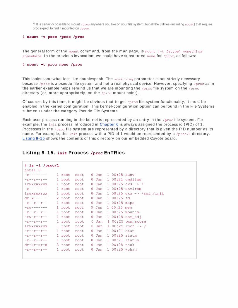
[6] It is certainly possible to mount /proc anywhere you like on your file system, but all the utilities (including mount) that require
proc expect to find it mounted on /proc.
$ mount -t proc /proc /proc
The general form of the mount command, from the man page, is mount [-t fstype] somethingsomewhere. In the previous invocation, we could have substituted none for /proc, as follows:
$ mount -t proc none /proc
This looks somewhat less like doublespeak. The something parameter is not strictly necessarybecause /proc is a pseudo file system and not a real physical device. However, specifying /proc as inthe earlier example helps remind us that we are mounting the /proc file system on the /procdirectory (or, more appropriately, on the /proc mount point).
Of course, by this time, it might be obvious that to get /proc file system functionality, it must beenabled in the kernel configuration. This kernel-configuration option can be found in the File Systemssubmenu under the category Pseudo File Systems.
Each user process running in the kernel is represented by an entry in the /proc file system. Forexample, the init process introduced in Chapter 6 is always assigned the process id (PID) of 1.Processes in the /proc file system are represented by a directory that is given the PID number as itsname. For example, the init process with a PID of 1 would be represented by a /proc/1 directory.Listing 9-15 shows the contents of this directory on our embedded Coyote board.
Listing 9-15. init Process /proc EnTRies
# ls -l /proc/1total 0-r-------- 1 root root 0 Jan 1 00:25 auxv-r--r--r-- 1 root root 0 Jan 1 00:21 cmdlinelrwxrwxrwx 1 root root 0 Jan 1 00:25 cwd -> /-r-------- 1 root root 0 Jan 1 00:25 environlrwxrwxrwx 1 root root 0 Jan 1 00:25 exe -> /sbin/initdr-x------ 2 root root 0 Jan 1 00:25 fd-r--r--r-- 1 root root 0 Jan 1 00:25 maps-rw------- 1 root root 0 Jan 1 00:25 mem-r--r--r-- 1 root root 0 Jan 1 00:25 mounts-rw-r--r-- 1 root root 0 Jan 1 00:25 oom_adj-r--r--r-- 1 root root 0 Jan 1 00:25 oom_scorelrwxrwxrwx 1 root root 0 Jan 1 00:25 root -> /-r--r--r-- 1 root root 0 Jan 1 00:21 stat-r--r--r-- 1 root root 0 Jan 1 00:25 statm-r--r--r-- 1 root root 0 Jan 1 00:21 statusdr-xr-xr-x 3 root root 0 Jan 1 00:25 task-r--r--r-- 1 root root 0 Jan 1 00:25 wchan

These entries, which are present in the /proc file system for each running process, contain muchuseful information, especially for analyzing and debugging a process. For example, the cmdline entrycontains the complete command line used to invoke the process, including any arguments. The cwdand root directories contain the processes' view of the current working directory and the current rootdirectory.
One of the more useful entries for system debugging is the maps entry. This contains a list of eachvirtual memory segment assigned to the program, along with attributes about each. Listing 9-16 isthe output from /proc/1/maps in our example of the init process.
Listing 9-16. init Process Memory Segments from /proc
# cat /proc/1/maps00008000-0000f000 r-xp 00000000 00:0a 9537567 /sbin/init00016000-00017000 rw-p 00006000 00:0a 9537567 /sbin/init00017000-0001b000 rwxp 00017000 00:00 040000000-40017000 r-xp 00000000 00:0a 9537183 /lib/ld-2.3.2.so40017000-40018000 rw-p 40017000 00:00 04001f000-40020000 rw-p 00017000 00:0a 9537183 /lib/ld-2.3.2.so40020000-40141000 r-xp 00000000 00:0a 9537518 /lib/libc-2.3.2.so40141000-40148000 ---p 00121000 00:0a 9537518 /lib/libc-2.3.2.so40148000-4014d000 rw-p 00120000 00:0a 9537518 /lib/libc-2.3.2.so4014d000-4014f000 rw-p 4014d000 00:00 0befeb000-bf000000 rwxp befeb000 00:00 0#
The usefulness of this information is readily apparent. You can see the program segments of the initprocess itself in the first two entries. You can also see the memory segments used by the sharedlibrary objects being used by the init process. The format is as follows:
vmstart-vmend attr pgoffset devname inode filename
Here, vmstart and vmend are the starting and ending virtual memory addresses, respectively; attrindicates memory region attributes, such as read, write, and execute, and tells whether this region isshareable; pgoffset is the page offset of the region (a kernel virtual memory parameter); anddevname, displayed as xx:xx, is a kernel representation of the device ID associated with this memoryregion. The memory regions that are not associated with a file are also not associated with a device,thus the 00:00. The final two entries are the inode and file associated with the given memory region.Of course, if there is no file, there is no inode associated with it, and it displays with a zero. These areusually data segments.
Other useful entries are listed for each process. The status entry contains useful status informationabout the running process, including items such as the parent PID, user and group IDs, virtualmemory usage stats, signals, and capabilities. More details can be obtained from the references atthe end of the chapter.
Some frequently used /proc enTRies are cpuinfo, meminfo, and version. The cpuinfo enTRy listsattributes that the kernel discovers about the processor(s) running on the system. The meminfo

enTRy provides statistics on the total system memory. The version entry mirrors the Linux kernelversion string, together with information on what compiler and machine were used to build thekernel.
Many more useful /proc entries are provided by the kernel; we have only scratched the surface ofthis useful subsystem. Many utilities have been designed for extracting and reporting informationcontained with the /proc file system. Two popular examples are top and ps, which every embeddedLinux developer should be intimately familiar with. These are introduced in Chapter 13. Other utilitiesuseful for interfacing with the /proc file system include free, pkill, pmap, and uptime. See the procpspackage for more details.
9.8.2. sysfs
Like the /proc file system, sysfs is not representative of an actual physical device. Instead, sysfsmodels specific kernel objects such as physical devices and provides a way to associate devices withdevice drivers. Some agents in a typical Linux distribution depend on the information on sysfs.
We can get some idea of what kinds of objects are exported by looking directly at the directorystructure exported by sysfs. Listing 9-17 shows the top-level /sys directory on our Coyote board.
Listing 9-17. Top-Level /sys Directory Contents
# dir /systotal 0drwxr-xr-x 21 root root 0 Jan 1 00:00 blockdrwxr-xr-x 6 root root 0 Jan 1 00:00 busdrwxr-xr-x 10 root root 0 Jan 1 00:00 classdrwxr-xr-x 5 root root 0 Jan 1 00:00 devicesdrwxr-xr-x 2 root root 0 Jan 1 00:00 firmwaredrwxr-xr-x 2 root root 0 Jan 1 00:00 kerneldrwxr-xr-x 5 root root 0 Jan 1 00:00 moduledrwxr-xr-x 2 root root 0 Jan 1 00:00 power#
As you can see, sysfs provides a subdirectory for each major class of system device, including thesystem buses. For example, under the block subdirectory, each block device is represented by asubdirectory entry. The same holds true for the other directories at the top level.
Most of the information stored by sysfs is in a format more suitable for machines than humans toread. For example, to discover the devices on the PCI bus, one could look directly at the/sys/bus/pci subdirectory. On our Coyote board, which has a single PCI device attached (an Ethernetcard), the directory looks like this:
# ls /sys/bus/pci/devices/0000:00:0f.0 -> ../../../devices/pci0000:00/0000:00:0f.0

This entry is actually a symbolic link pointing to another node in the sysfs directory tree. We haveformatted the output of ls here to illustrate this, while still fitting in a single line. The name of thesymbolic link is the kernel's representation of the PCI bus, and it points to a devices subdirectorycalled pci0000:00 (the PCI bus representation), which contains a number of subdirectories and filesrepresenting attributes of this specific PCI device. As you can see, the data is rather difficult todiscover and parse.
A useful utility exists to browse the sysfs file system directory structure. Called systool, it comesfrom the sysfsutils package found on sourceforge.net. Here is how systool would display the PCI busfrom the previous discussion:
$ systool -b pci Bus = "pci" 0000:00:0f.0 8086:1229
Again we see the kernel's representation of the bus and device (0f), but this time the tool displaysthe vendor ID (8086 = Intel) and device ID (1229 = eepro100 Ethernet card) obtained from the/sys/devices/pci0000:00 branch of /sys where these attributes are kept. Executed with noparameters, systool displays the top-level system hierarchy. Listing 9-18 is an example from ourCoyote board.
Listing 9-18. Output from systool
$ systoolSupported sysfs buses: i2c ide pci platformSupported sysfs classes: block i2c-adapter i2c-dev input mem misc net pci_bus ttySupported sysfs devices: pci0000:00 platform system
You can see from this listing the variety of system information available from sysfs. Many utilities usethis information to determine the characteristics of system devices or to enforce system policies, suchas power management and hot-plug capability.


9.9. Other File Systems
Numerous file systems are supported under Linux. Space does not permit coverage of all of them.However, you should be aware of some other important file systems frequently found in embeddedsystems.
The ramfs file system is best considered from the context of the Linux source code module thatimplements it. Listing 9-19 reproduces the first several lines of that file.
Listing 9-19. Linux ramfs Source Module Comments
/* * Resizable simple ram filesystem for Linux. * * Copyright (C) 2000 Linus Torvalds. * 2000 Transmeta Corp. * * Usage limits added by David Gibson, Linuxcare Australia. * This file is released under the GPL. */
/* * NOTE! This filesystem is probably most useful * not as a real filesystem, but as an example of * how virtual filesystems can be written. * * It doesn't get much simpler than this. Consider * that this file implements the full semantics of * a POSIX-compliant read-write filesystem.
This module was written primarily as an example of how virtual file systems can be written. One ofthe primary differences between this file system and the ramdisk facility found in modern Linuxkernels is its capability to shrink and grow according to its use. A ramdisk does not have thisproperty. This source module is compact and well written. It is presented here for its educationalvalue. You are encouraged to study this good example.
The tmpfs file system is similar to and related to rams. Like ramfs, everything in tmpfs is stored inkernel virtual memory, and the contents of tmpfs are lost on power-down or reboot. The tmpfs filesystem is useful for fast temporary storage of files. I use tmpfs mounted on /tmp in a midi/audioapplication to speed up the creation and deletion of temporary objects required by the audiosubsystem. This is also a great way to keep your /tmp directory cleanits contents are lost on everyreboot. Mounting tmpfs is similar to any other virtual file system:
# mount -t tmpfs /tmpfs /tmp

As with other virtual file systems such as /proc, the first /tmpfs parameter in the previous mountcommand is a "no-op"that is, it could be the word none and still function. However, it is a goodreminder that you are mounting a virtual file system called tmpfs.

9.10. Building a Simple File System
It is straightforward to build a simple file system image. Here we demonstrate the use of the Linuxkernel's loopback device. The loopback device enables the use of a regular file as a block device. Inshort, we build a file system image in a regular file and use the Linux loopback device to mount thatfile in the same way any other block device is mounted.
To build a simple root file system, start with a fixed-sized file containing all zeros:
# dd if=/dev/zero of=./my-new-fs-image bs=1k count=512
This command creates a file of 512KB containing nothing but zeros. We fill the file with zeros to aid incompression later and to have a consistent data pattern for uninitialized data blocks within the filesystem. Use caution with the dd command. Executing dd with no boundary (count=) or with animproper boundary can fill up your hard drive and possibly crash your system. dd is a powerful tool;use it with the respect it deserves. Simple typos in commands such as dd, executed as root, havedestroyed countless file systems.
When we have the new image file, we actually format the file to contain the data structures definedby a given file system. In this example, we build an ext2 file system. Listing 9-20 details theprocedure.
Listing 9-20. Creating an ext2 File System Image
# /sbin/mke2fs ./my-new-fs-imagemke2fs 1.35 (28-Feb-2004)./my-new-fs-image is not a block special device.Proceed anyway? (y,n) yFilesystem label=OS type: LinuxBlock size=1024 (log=0)Fragment size=1024 (log=0)64 inodes, 512 blocks25 blocks (4.88%) reserved for the super userFirst data block=11 block group8192 blocks per group, 8192 fragments per group64 inodes per group
Writing inode tables: doneWriting superblocks and filesystem accounting information: done
This filesystem will be automatically checked every 24 mounts or180 days, whichever comes first. Use tune2fs -c or -i to override.

#
As with dd, the mke2fs command can destroy your system, so use it with care. In this example, weasked mke2fs to format a file rather than a hard drive partition (block device) for which it wasintended. As such, mke2fs detected that fact and asked us to confirm the operation. After confirming,mke2fs proceeded to write an ext2 superblock and file system data structures into the file. We thencan mount this file like any block device, using the Linux loopback device:
# mount -o loop ./my-new-fs-image /mnt/flash
This command mounts the file my-new-fs-image as a file system on the mount point named/mnt/flash. The mount point name is not important; you can mount it wherever you want, as long asthe mount point exists. Use mkdir to create your mount point.
After the newly created image file is mounted as a file system, we are free to make changes to it. Wecan add and delete directories, make device nodes, and so on. We can use tar to copy files into orout of it. When the changes are complete, they are saved in the file, assuming that you didn't exceedthe size of the device. Remember, using this method, the size is fixed at creation time and cannot bechanged.

9.11. Chapter Summary
Partitions are the logical division of a physical device. Numerous partition types are supportedunder Linux.
A file system is mounted on a mount point in Linux. The root file system is mounted at the rootof the file system hierarchy and referred to as /.
The popular ext2 file system is mature and fast, and is often found on embedded and otherLinux systems such as Red Hat and the Fedora Core series.
The ext3 file system adds journaling on top of the ext2 file system, for better data integrity andsystem reliability.
ReiserFS is another popular and high-performance journaling file system found on manyembedded and other Linux systems.
JFFS2 is a journaling file system optimized for use with Flash memory. It contains Flash-friendlyfeatures such as wear leveling for longer Flash memory lifetime.
cramfs is a read-only file system perfect for small-system boot ROMs and other read-onlyprograms and data.
NFS is one of the most powerful development tools for the embedded developer. It can bringthe power of a workstation to your target device. Learn how to use NFS as your embeddedtarget's root file system. The convenience and time savings will be worth the effort.
Many pseudo file systems are available on Linux. A few of the more important ones arepresented here, including the proc file system and sysfs.
The RAM-based tmpfs file system has many uses for embedded systems. Its most significantimprovement over traditional ramdisks is the capability to resize itself dynamically to meetoperational requirements.
9.11.1. Suggestions for Additional Reading
"Design and Implementation of the Second Extended Filesystem"Rémy Card, Theodore Ts'o, and Stephen TweedieFirst published in the Proceedings of the First DutchInternational Symposium on LinuxAvailable on http://e2fsprogs.sourceforge.net/ext2intro.html
"A Non-Technical Look Inside the EXT2 File System"Randy Appletonwww.linuxgazette.com/issue21/ext2.html

Whitepaper: Red Hat's New Journaling File System: ext3Michael K. Johnsonwww.redhat.com/support/wpapers/redhat/ext3/
ReiserFS Home Pagewww.namesys.com/
"JFFS: The Journaling Flash File System"David Woodhousehttp://sources.redhat.com/jffs2/jffs2.pdf
README file from cramfs projectUnsigned (assumed to be the project author)http://sourceforge.net/projects/cramfs/
NFS home pagehttp://nfs.sourceforge.net
The /proc file system documentationwww.tldp.org/LDP/lkmpg/2.6/html/c712.htm
File System Performance: The Solaris OS, UFS, Linux ext3, and ReiserFSA technical whitepaperDominic Kaywww.sun.com/software/whitepapers/solaris10/fs_performance.pdf

Chapter 10. MTD SubsystemIn this chapter
Enabling MTD Services page 248
MTD Basics page 251
MTD Partitions page 253
MTD Utilities page 265
Chapter Summary page 270
The Memory Technology Devices (MTD) subsystem grew out of the need to support a wide variety ofmemory-like devices such as Flash memory chips. Many different types of Flash chips are available,along with numerous methods to program them, partly because of the many specialized and high-performance modes that are supported. The MTD layer architecture enables the separation of thelow-level device complexities from the higher-layer data organization and storage formats that usememory devices.
In this chapter, we introduce the MTD subsystem and provide some simple examples of its use. Firstwe look at what is required of the kernel to support MTD services. We introduce some simpleoperations on a development workstation with MTD enabled, as a means to understand the basics ofthis subsystem. In this chapter, we integrate MTD and the JFFS2 file system.
We next introduce the concept of partitions as they relate to the MTD layer. We examine the detailsof building partitions from a bootloader and how they are detected by the Linux kernel. The chaptercontinues with a brief introduction to the MTD utilities. We conclude by putting it all together andbooting a target board using an in-Flash JFFS2 file system image.

10.1. Enabling MTD Services
To use MTD services, your kernel must be configured with MTD enabled. Many configuration optionsexist for MTD, some of which can be confusing. The best way to understand the myriad choices issimply to begin working with them. To illustrate the mechanics of the MTD subsystem and how it fitsin with the system, we begin with some very simple examples that you can perform on your Linuxdevelopment workstation. Figure 10-1 shows the kernel configuration (invoked per the usual makeARCH=<arch> gconfig) necessary to enable the bare-minimum MTD functionality. Listing 10-1 displaysthe .config file entries resulting from the selections shown in Figure 10-1.
Listing 10-1. Basic MTD Configuration from .config
CONFIG_MTD=yCONFIG_MTD_CHAR=yCONFIG_MTD_BLOCK=yCONFIG_MTD_MTDRAM=mCONFIG_MTDRAM_TOTAL_SIZE=8192CONFIG_MTDRAM_ERASE_SIZE=128
The MTD subsystem is enabled via the first configuration option, which is selected via the first checkbox shown in Figure 10-1, Memory Technology Device (MTD) Support. The next two entries from theconfiguration shown in Figure 10-1 enable special device-level access to the MTD devices, such asFlash memory, from user space. The first one (CONFIG_MTD_CHAR) enables character device modeaccess, essentially a sequential access characterized by byte-at-a-time sequential read and writeaccess. The second (CONFIG_MTD_BLOCK) enables access to the MTD device in block device mode, theaccess method used for disk drives, in which blocks of multiple bytes of data are read or written at atime. These access modes allow the use of familiar Linux commands to read and write data to theFlash memory, as you shall shortly see.
Figure 10-1. MTD configuration
[View full size image]

The CONFIG_MTD_MTDRAM element enables a special test driver that enables us to examine the MTDsubsystem even if we don't have any MTD devices (such as Flash memory) available. Coupled withthis configuration selection are two parameters associated with the RAM-based test driver: the devicesize and the erase size. For this example, we have specified 8192KB total size and 128KB erase size.The objective of this test driver is to emulate a Flash device, primarily to facilitate MTD subsystemtesting and development. Because Flash memory is architected using fixed-size erase blocks, the testdriver also contains the concept of erase blocks. You will see how these parameters are used shortly.
10.1.1. Building MTD
MTD is included in any recent snapshot of the Linux kernel. However, if you need to take advantageof MTD features that have been added since your kernel version was released, you must downloadand build the MTD drivers and utilities. Because the MTD package contains both kernel componentsand user space programs, it is useful to keep the MTD package in a separate project directory andconnect it to your kernel source tree. The simplest way to integrate the MTD and your kernel sourcetree(s) is to use the scripts provided by the MTD package.
Download the MTD package from the location given at the end of this chapter. Unpack the archiveinto a directory of your choice using the tar utility. Enter the directory and run the patchkernel.shscript. This script provides several options. Execute the script with no parameters for a detailedusage. Listing 10-2 shows how to install the kernel components.
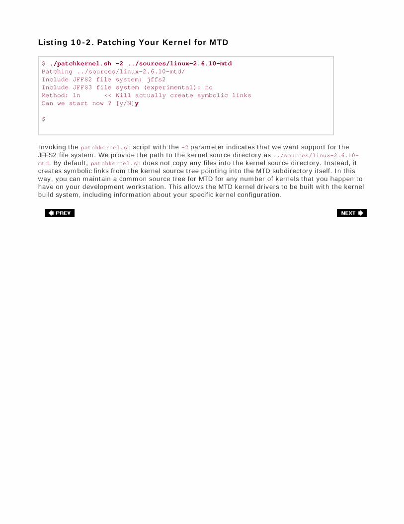
Listing 10-2. Patching Your Kernel for MTD
$ ./patchkernel.sh -2 ../sources/linux-2.6.10-mtdPatching ../sources/linux-2.6.10-mtd/Include JFFS2 file system: jffs2Include JFFS3 file system (experimental): noMethod: ln << Will actually create symbolic linksCan we start now ? [y/N]y
$
Invoking the patchkernel.sh script with the -2 parameter indicates that we want support for theJFFS2 file system. We provide the path to the kernel source directory as ../sources/linux-2.6.10-mtd. By default, patchkernel.sh does not copy any files into the kernel source directory. Instead, itcreates symbolic links from the kernel source tree pointing into the MTD subdirectory itself. In thisway, you can maintain a common source tree for MTD for any number of kernels that you happen tohave on your development workstation. This allows the MTD kernel drivers to be built with the kernelbuild system, including information about your specific kernel configuration.
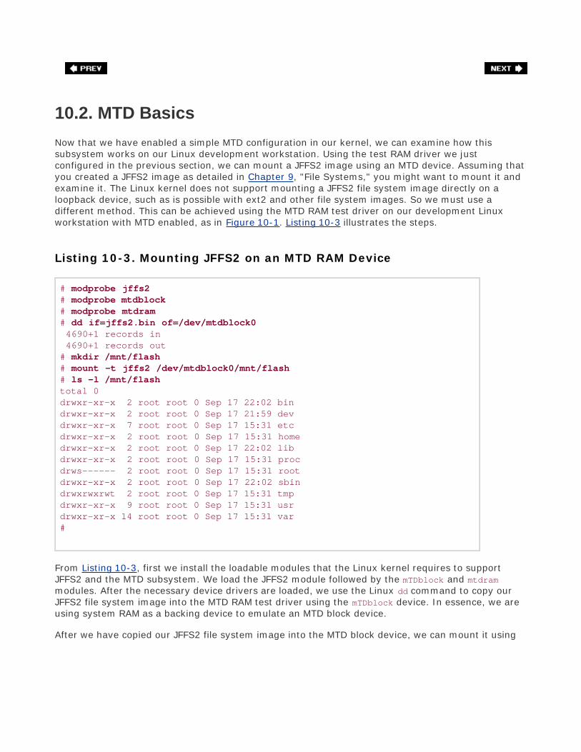
10.2. MTD Basics
Now that we have enabled a simple MTD configuration in our kernel, we can examine how thissubsystem works on our Linux development workstation. Using the test RAM driver we justconfigured in the previous section, we can mount a JFFS2 image using an MTD device. Assuming thatyou created a JFFS2 image as detailed in Chapter 9, "File Systems," you might want to mount it andexamine it. The Linux kernel does not support mounting a JFFS2 file system image directly on aloopback device, such as is possible with ext2 and other file system images. So we must use adifferent method. This can be achieved using the MTD RAM test driver on our development Linuxworkstation with MTD enabled, as in Figure 10-1. Listing 10-3 illustrates the steps.
Listing 10-3. Mounting JFFS2 on an MTD RAM Device
# modprobe jffs2# modprobe mtdblock# modprobe mtdram# dd if=jffs2.bin of=/dev/mtdblock0 4690+1 records in 4690+1 records out# mkdir /mnt/flash# mount -t jffs2 /dev/mtdblock0/mnt/flash# ls -l /mnt/flashtotal 0drwxr-xr-x 2 root root 0 Sep 17 22:02 bindrwxr-xr-x 2 root root 0 Sep 17 21:59 devdrwxr-xr-x 7 root root 0 Sep 17 15:31 etcdrwxr-xr-x 2 root root 0 Sep 17 15:31 homedrwxr-xr-x 2 root root 0 Sep 17 22:02 libdrwxr-xr-x 2 root root 0 Sep 17 15:31 procdrws------ 2 root root 0 Sep 17 15:31 rootdrwxr-xr-x 2 root root 0 Sep 17 22:02 sbindrwxrwxrwt 2 root root 0 Sep 17 15:31 tmpdrwxr-xr-x 9 root root 0 Sep 17 15:31 usrdrwxr-xr-x 14 root root 0 Sep 17 15:31 var#
From Listing 10-3, first we install the loadable modules that the Linux kernel requires to supportJFFS2 and the MTD subsystem. We load the JFFS2 module followed by the mTDblock and mtdrammodules. After the necessary device drivers are loaded, we use the Linux dd command to copy ourJFFS2 file system image into the MTD RAM test driver using the mTDblock device. In essence, we areusing system RAM as a backing device to emulate an MTD block device.
After we have copied our JFFS2 file system image into the MTD block device, we can mount it using

the mount command, in the manner shown in Listing 10-3. After the MTD pseudo-device has beenmounted, we can work with the JFFS2 file system image in any way we choose. The only limitationusing this method is that we can't enlarge the image. The size of the image is limited by two factors.First, when we configured the MTD RAM test device, we gave it a maximum size of 8MB.[1] Second,when we created the JFFS2 image, we fixed the size of the image using the mkfs.jffs2 utility. Theimage size was determined by the contents of the directory we specified when we created it. Referback to Listing 9-9, in Chapter 9, to recall how our jffs2.bin image was built.
[1] The size was fixed in the kernel configuration when we enabled the MTD RAM test device in the Linux kernel configuration.
It is important to realize the limitations of using this method to examine the contents of a JFFS2 filesystem. Consider what we did: We copied the contents of a file (the JFFS2 file system binary image)into a kernel block device (/dev/mtdblock0). Then we mounted the kernel block device(/dev/mtdblock) as a JFFS2 file system. After we did this, we could use all the traditional file systemutilities to examine and even modify the file system. Tools such as ls,df,dh,mv,rm, and cp can all beused to examine and modify the file system. However, unlike the loopback device, there is noconnection between the file we copied and the mounted JFFS2 file system image. Therefore, if weunmount the file system after making changes, the changes will be lost. If you want to save thechanges, you must copy them back into a file. One such method is the following:
# dd if=/dev/mtdblock0 of=./your-modified-fs-image.bin
This command creates a file called your-modified-fs-image.bin that is the same size as themtdblock0 device which was specified during configuration. In our example, it would be 8MB. Lackingsuitable JFFS2 editing facilities, this is a perfectly valid way to examine and modify a JFFS2 filesystem. More important, it illustrates the basics of the MTD subsystem on our development systemwithout real Flash memory. Now let's look at some hardware that contains Flash physical devices.
10.2.1. Configuring MTD
To use MTD with the Flash memory on your board, you must have MTD configured correctly. Thefollowing list contains the requirements that must be satisfied to configure MTD for your board, Flash,and Flash layout.
Specify the partitioning on your Flash device
Specify the type of Flash and location
Configure the proper Flash driver for your chosen chip
Configure the kernel with the appropriate driver(s)
Each of these steps is explored in the following sections.

10.3. MTD Partitions
Most Flash devices on a given hardware platform are divided into several sections, called partitions,similar to the partitions found on a typical desktop workstation hard drive. The MTD subsystemprovides support for such Flash partitions. The MTD subsystem must be configured for MTDpartitioning support. Figure 10-2 illustrates the configuration options for MTD partitioning support.
Figure 10-2. Kernel configuration for MTD partitioning support
[View full size image]

Several methods exist for communicating the partition data to the Linux kernel. The followingmethods are currently supported. You can see the configuration options for each in Figure 10-2 underMTD Partitioning Support.
Redboot partition table parsing
Kernel command-line partition table definition
Board-specific mapping drivers
MTD also allows configurations without partition data. In this case, MTD simply treats the entire Flashmemory as a single device.
10.3.1. Redboot Partition Table Partitioning
One of the more common methods of defining and detecting MTD partitions stems from one of theoriginal implementations: Redboot partitions. Redboot is a bootloader found on many embeddedboards, especially ARM XScale boards such as the ADI Engineering Coyote Reference Platform.
The MTD subsystem defines a method for storing partition information on the Flash device itself,similar in concept to a partition table on a hard disk. In the case of the Redboot partitions, thedeveloper reserves and specifies a Flash erase block that holds the partition definitions. A mappingdriver is selected that calls the partition parsing functions during boot to detect the partitions on theFlash device. Figure 10-2 shows the mapping driver for our example board; it is the final highlightedentry defining CONFIG_MTD_IXP4xx.
As usual, taking a detailed look at an example helps to illustrate these concepts. We start by lookingat the information provided by the Redboot bootloader for the Coyote platform. Listing 10-4 capturessome of the output of the Redboot bootloader upon power-up.
Listing 10-4. Redboot Messages on Power-Up
Platform: ADI Coyote (XScale)IDE/Parallel Port CPLD Version: 1.0Copyright (C) 2000, 2001, 2002, Red Hat, Inc.
RAM: 0x00000000-0x04000000, 0x0001f960-0x03fd1000 availableFLASH: 0x50000000 - 0x51000000, 128 blocks of 0x00020000 bytes each....
This tells us that RAM on this board is physically mapped starting at address 0x00000000 and thatFlash is mapped at physical address 0x50000000 through 0x51000000. We can also see that theFlash has 128 blocks of 0x00020000 (128KB) each.
Redboot contains a command to create and display partition information on the Flash. Listing 10-5

contains the output of the fis list command, part of the Flash Image System family of commandsavailable in the Redboot bootloader.
Listing 10-5. Redboot Flash Partition List
RedBoot> fis listName FLASH addr Mem addr Length Entry pointRedBoot 0x50000000 0x50000000 0x00060000 0x00000000RedBoot config 0x50FC0000 0x50FC0000 0x00001000 0x00000000FIS directory 0x50FE0000 0x50FE0000 0x00020000 0x00000000RedBoot>
From Listing 10-5, we see that the Coyote board has three partitions defined on the Flash. Thepartition named RedBoot contains the executable Redboot bootloader image. The partition namedRedBoot config contains the configuration parameters maintained by the bootloader. The finalpartition named FIS directory holds information about the partition table itself.
When properly configured, the Linux kernel can detect and parse this partition table and create MTDpartitions representing the physical partitions on Flash. Listing 10-6 reproduces a portion of the bootmessages that are output from the aforementioned ADI Engineering Coyote board, booting a Linuxkernel configured with support for detecting Redboot partitions.
Listing 10-6. Detecting Redboot Partitions on Linux Boot
...IXP4XX-Flash0: Found 1 x16 devices at 0x0 in 16-bit bank Intel/Sharp Extended Query Table at 0x0031Using buffer write methodcfi_cmdset_0001: Erase suspend on write enabledSearching for RedBoot partition table in IXP4XX-Flash0 at offset 0xfe00003 RedBoot partitions found on MTD device IXP4XX-Flash0Creating 3 MTD partitions on "IXP4XX-Flash0":0x00000000-0x00060000: "RedBoot"0x00fc0000-0x00fc1000: "RedBoot config"0x00fe0000-0x01000000: "FIS directory"...
The first message in Listing 10-6 is printed when the Flash chip is detected, via the Common FlashInterface (CFI) driver, enabled via CONFIG_MTD_CFI. CFI is an industry-standard method fordetermining the Flash chip's characteristics, such as manufacturer, device type, total size, and eraseblock size. See Section 10.5.1, "Suggestions for Additional Reading," at the end of this chapter for apointer to the CFI specification.
CFI is enabled via the kernel-configuration utility under the Memory Technology Devices (MTD) top-level menu. Select Detect flash chips by Common Flash Interface (CFI) probe under

RAM/ROM/Flash chip drivers, as illustrated in Figure 10-3.
Figure 10-3. Kernel configuration for MTD CFI support
[View full size image]
As shown in Listing 10-6, the Flash chip is detected via the CFI interface. Because we also enabledCONFIG_MTD_REDBOOT_PARTS (see Figure 10-2), MTD scans for the Redboot partition table on the Flashchip. Notice also that the chip has been enumerated with the device name IXP4XX-Flash0. You cansee from Listing 10-6 that the Linux kernel has detected three partitions on the Flash chip, asenumerated previously using the fis list command in Redboot.
When the infrastructure is in place as described here, the Linux kernel automatically detects andcreates kernel data structures representing the three Flash partitions. Evidence of these can be foundin the /proc file system when the kernel has completed initialization, as shown in Listing 10-7.
Listing 10-7. Kernel MTD Flash Partitions

root@coyote:~# cat /proc/mtddev: size erasesize namemtd0: 00060000 00020000 "RedBoot"mtd1: 00001000 00020000 "RedBoot config"mtd2: 00020000 00020000 "FIS directory"#
We can easily create a new Redboot partition. We use the Redboot FIS commands for this example,but we do not detail the Redboot commands in this book. However, the interested reader can consultthe Redboot user documentation listed in Section 10.5.1 at the end of this chapter. Listing 10-8shows the details of creating a new Redboot partition.
Listing 10-8. Creating a New Redboot Partition
RedBoot> load -r -v -b 0x01008000 coyote-40-zImageUsing default protocol (TFTP)Raw file loaded 0x01008000-0x0114dccb, assumed entry at 0x01008000RedBoot> fis create -b 0x01008000 -l 0x145cd0 -f 0x50100000 MyKernel... Erase from 0x50100000-0x50260000: .............. Program from 0x01008000-0x0114dcd0 at 0x50100000: .............. Unlock from 0x50fe0000-0x51000000: .... Erase from 0x50fe0000-0x51000000: .... Program from 0x03fdf000-0x03fff000 at 0x50fe0000: .... Lock from 0x50fe0000-0x51000000: .
First, we load the image we will use to create the new partition. We will use our kernel image for theexample. We load it to memory address 0x01008000. Then we create the new partition using theRedboot fis create command. We have instructed Redboot to create the new partition in an area ofFlash starting at 0x50100000. You can see the action as Redboot first erases this area of Flash andthen programs the kernel image. In the final sequence, Redboot unlocks its directory area andupdates the FIS Directory with the new partition information. Listing 10-9 shows the output of fislist with the new partition. Compare this with the output in Listing 10-5.
Listing 10-9. New Redboot Partition List
RedBoot> fis listName FLASH addr Mem addr Length Entry pointRedBoot 0x50000000 0x50000000 0x00060000 0x00000000RedBoot config 0x50FC0000 0x50FC0000 0x00001000 0x00000000FIS directory 0x50FE0000 0x50FE0000 0x00020000 0x00000000MyKernel 0x50100000 0x50100000 0x00160000 0x01008000
Of course, when we boot the Linux kernel, it discovers the new partition and we can operate on it as

we see fit. The astute reader might have realized the other benefit of this new partition: We can nowboot the kernel from Flash instead of having to load it via tftp every time. The command isillustrated next. Simply pass the Redboot exec command the Flash starting address of the partitionand the length of the image to transfer into RAM.
RedBoot> exec -b 0x50100000 -l 0x145cd0 Uncompressing Linux........... done, booting the kernel....
10.3.2. Kernel Command Line Partitioning
As detailed in Section 10.3, "MTD Partitions," the raw Flash partition information can becommunicated to the kernel using other methods. Indeed, possibly the most straightforward, thoughperhaps not the simplest method is to manually pass the partition information directly on the kernelcommand line. Of course, as we have already learned, some bootloaders make that easy (forexample U-Boot), whereas others do not have a facility to pass a kernel command line to the kernelupon boot. In these cases, the kernel command line must be configured at compile time and,therefore, is more difficult to change, requiring a recompile of the kernel itself each time thepartitions are modified.
To enable command-line partitioning in the MTD subsystem, your kernel must be configured for thissupport. You can see this configuration option in Figure 10-2 under MTD partitioning support. Selectthe option for command-line partition table parsing, which defines the CONFIG_MTD_CMDLINE_PARTSoption.
Listing 10-10 shows the format for defining a partition on the kernel command line (taken from.../drivers/mtd/cmdlinepart.c).
Listing 10-10. Kernel Command-Line MTD Partition Format
mtdparts=<mtddef>[;<mtddef] *<mtddef> := <mtd-id>:<partdef>[,<partdef>] *<partdef> := <size>[@offset][<name>][ro] *<mtd-id> := unique name used in mapping driver/device (mtd->name) *<size> := std linux memsize OR "-" to denote all remaining space *<name> := '(' NAME ')'
Each mtddef parameter passed on the kernel command line defines a separate partition. As shown isListing 10-10, each mtddef definition contains multiple parts. You can specify a unique ID, partitionsize, and offset from the start of the Flash. You can also pass the partition a name and, optionally,the read-only attribute. Referring back to our Redboot partition definitions in Listing 10-5, we couldstatically define these on the kernel command line as follows:
mtdparts=MainFlash:384K(Redboot),4K(config),128K(FIS),-(unused)
With this definition, the kernel would instantiate four MTD partitions, with an MTD ID of MainFlash,

containing the sizes and layout matching that found in Listing 10-5.
10.3.3. Mapping Driver
The final method for defining your board-specific Flash layout is to use a dedicated board-specificmapping driver. The Linux kernel source tree contains many examples of mapping drivers, located in.../drivers/mtd/maps. Any one of these will provide good examples for how to create your own. Theimplementation details vary by architecture.
The mapping driver is a proper kernel module, complete with module_init() and module_exit() calls,as described in Chapter 8, "Device Driver Basics." A typical mapping driver is small and easy tonavigate, often containing fewer than a couple dozen lines of C.
Listing 10-11 reproduces a section of .../drivers/mtd/maps/pq2fads. This mapping driver defines theFlash device on a Freescale PQ2FADS evaluation board that supports the MPC8272 and otherprocessors.
Listing 10-11. PQ2FADs Flash Mapping Driver
...static struct mtd_partition pq2fads_partitions[] = { {#ifdef CONFIG_ADS8272 .name = "HRCW", .size = 0x40000, .offset = 0, .mask_flags= MTD_WRITEABLE, /* force read-only */ }, { .name = "User FS", .size = 0x5c0000, .offset = 0x40000,#else .name = "User FS", .size = 0x600000, .offset = 0,#endif }, { .name = "uImage", .size = 0x100000, .offset = 0x600000, .mask_flags = MTD_WRITEABLE, /* force read-only */ }, { .name = "bootloader", .size = 0x40000, .offset = 0x700000, .mask_flags = MTD_WRITEABLE, /* force read-only */ }, { .name = "bootloader env", .size = 0x40000,

.offset = 0x740000, .mask_flags = MTD_WRITEABLE, /* force read-only */ }};/* pointer to MPC885ADS board info data */extern unsigned char __res[];
static int __init init_pq2fads_mtd(void){ bd_t *bd = (bd_t *)__res; physmap_configure(bd->bi_flashstart, bd->bi_flashsize, PQ2FADS_BANK_WIDTH, NULL);
physmap_set_partitions(pq2fads_partitions, sizeof (pq2fads_partitions) / sizeof (pq2fads_partitions[0])); return 0;}
static void __exit cleanup_pq2fads_mtd(void){}module_init(init_pq2fads_mtd);module_exit(cleanup_pq2fads_mtd);...
This simple but complete Linux device driver communicates the PQ2FADS Flash mapping to the MTDsubsystem. Recall from Chapter 8 that when a function in a device driver is declared with themodule_init() macro, it is automatically invoked during Linux kernel boot at the appropriate time. Inthis PQ2FADS mapping driver, the module initialization function init_pq2fads_mtd() performs justtwo simple calls:
physmap_configure() passes to the MTD subsystem the Flash chip's physical address, size,and bank width, along with any special setup function required to access the Flash.
physmap_set_partitions() passes the board's unique partition information to the MTDsubsystem from the partition table defined in the pq2fads_partitions[] array found at thestart of this mapping driver.
Following this simple example, you can derive a mapping driver for your own board.
10.3.4. Flash Chip Drivers
MTD has support for a wide variety of Flash chips and devices. Chances are very good that yourchosen chip has also been supported. The most common Flash chips support the Common FlashInterface (CFI) mentioned earlier. Older Flash chips might have JEDEC support, which is an olderFlash compatibility standard. Figure 10-4 shows the kernel configuration from a recent Linux kernelsnapshot. This version supports many Flash types.

Figure 10-4. Flash device support
[View full size image]
If your Flash chip is not supported, you must provide a device file yourself. Using one of the manyexamples in .../drivers/mtd/chips as a starting point, customize or create your own Flash devicedriver. Better yet, unless the chip was just introduced with some newfangled interface, chances aregood that someone has already produced a driver.
10.3.5. Board-Specific Initialization

Along with a mapping driver, your board-specific (platform) setup must provide the underlyingdefinitions for proper MTD Flash system operation. Listing 10-12 reproduces the relevant portions of.../arch/arm/mach-ixp4xx/coyote-setup.c.
Listing 10-12. Coyote-Specific Board Setup
static struct flash_platform_data coyote_flash_data = { .map_name = "cfi_probe", .width = 2,};
static struct resource coyote_flash_resource = { .start = COYOTE_FLASH_BASE, .end = COYOTE_FLASH_BASE + COYOTE_FLASH_SIZE - 1, .flags = IORESOURCE_MEM,};
static struct platform_device coyote_flash = { .name = "IXP4XX-Flash", .id = 0, .dev = { .platform_data = &coyote_flash_data, }, .num_resources = 1, .resource = &coyote_flash_resource,};
...
static struct platform_device *coyote_devices[] __initdata = { &coyote_flash, &coyote_uart};
static void __init coyote_init(void){ ...
platform_add_devices(coyote_devices, ARRAY_SIZE(coyote_devices));}...
In Listing 10-12, only the relevant portions of the coyote-setup.c platform initialization file arereproduced. Starting from the bottom, the coyote_init() function calls platform_add_devices(),specifying the Coyote-specific devices defined earlier in this file. You'll notice that two devices aredefined just above the coyote_init() routine. The one we're interested in for this discussion iscoyote_flash. This structure of type struct platform_device contains all the important detailsneeded by the Linux kernel and MTD subsystem.

The .name member of the coyote_flash structure binds our platform-specific Flash resource to amapping driver with the same name. You can see this in the mapping driver file.../drivers/mtd/maps/ixp4xx.c. The .resource member communicates the base address of the Flashon the board. The .dev member, which contains a .platform_data member, ties our Flash setup to achip driver. In this case, we have specified that our board will use the CFI probe method, specified inthe kernel configuration as CONFIG_MTD_CFI. You can see this configuration selection in Figure 10-4.
Depending on your own architecture and board, you can use a method similar to this to define theFlash support for your own board.
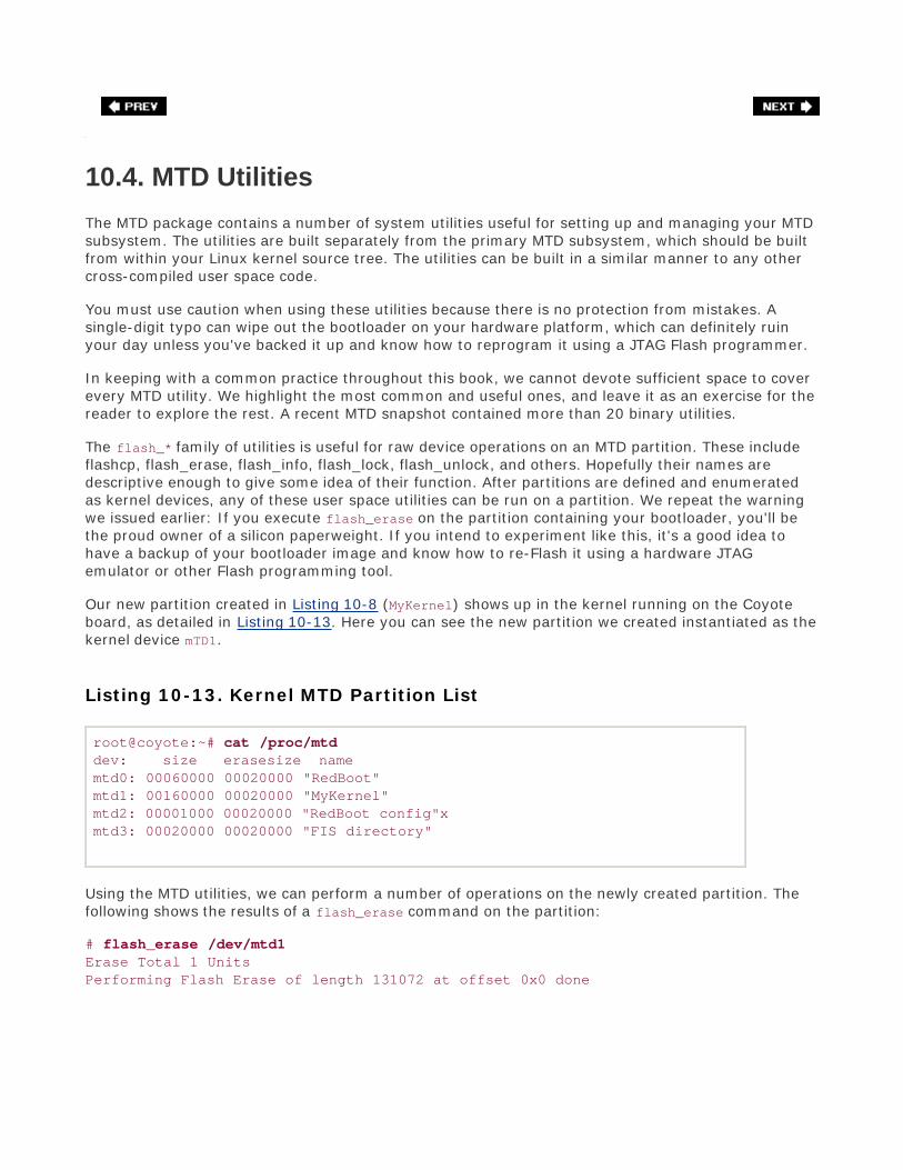
10.4. MTD Utilities
The MTD package contains a number of system utilities useful for setting up and managing your MTDsubsystem. The utilities are built separately from the primary MTD subsystem, which should be builtfrom within your Linux kernel source tree. The utilities can be built in a similar manner to any othercross-compiled user space code.
You must use caution when using these utilities because there is no protection from mistakes. Asingle-digit typo can wipe out the bootloader on your hardware platform, which can definitely ruinyour day unless you've backed it up and know how to reprogram it using a JTAG Flash programmer.
In keeping with a common practice throughout this book, we cannot devote sufficient space to coverevery MTD utility. We highlight the most common and useful ones, and leave it as an exercise for thereader to explore the rest. A recent MTD snapshot contained more than 20 binary utilities.
The flash_* family of utilities is useful for raw device operations on an MTD partition. These includeflashcp, flash_erase, flash_info, flash_lock, flash_unlock, and others. Hopefully their names aredescriptive enough to give some idea of their function. After partitions are defined and enumeratedas kernel devices, any of these user space utilities can be run on a partition. We repeat the warningwe issued earlier: If you execute flash_erase on the partition containing your bootloader, you'll bethe proud owner of a silicon paperweight. If you intend to experiment like this, it's a good idea tohave a backup of your bootloader image and know how to re-Flash it using a hardware JTAGemulator or other Flash programming tool.
Our new partition created in Listing 10-8 (MyKernel) shows up in the kernel running on the Coyoteboard, as detailed in Listing 10-13. Here you can see the new partition we created instantiated as thekernel device mTD1.
Listing 10-13. Kernel MTD Partition List
root@coyote:~# cat /proc/mtddev: size erasesize namemtd0: 00060000 00020000 "RedBoot"mtd1: 00160000 00020000 "MyKernel"mtd2: 00001000 00020000 "RedBoot config"xmtd3: 00020000 00020000 "FIS directory"
Using the MTD utilities, we can perform a number of operations on the newly created partition. Thefollowing shows the results of a flash_erase command on the partition:
# flash_erase /dev/mtd1Erase Total 1 UnitsPerforming Flash Erase of length 131072 at offset 0x0 done

To copy a new kernel image to this partition, use the flashcp command:
root@coyote:~# flashcp /workspace/coyote-40-zImage /dev/mtd1
It gets a bit more interesting working with a root file system partition. We have the option of usingthe bootloader or the Linux kernel to place the initial image on the Redboot flash partition. First, weuse Redboot to create the new partition that will hold our root file system. The following commandcreates a new partition on the Flash called RootFS starting at physical memory 0x50300000, with alength of 30 blocks. Remember, a block, generically called an erase unit, is 128KB on this Flash chip.
RedBoot> fis create -f 0x50300000 -l 0x600000 -n RootFS
Next, we boot the kernel and copy the root file system image into the new partition we have namedRootFS. This is accomplished with the following command from a Linux command prompt on yourtarget board. Note that this assumes you have already placed your file system image in a directoryaccessible to your board. As mentioned many times throughout this book, NFS is your best choice fordevelopment.
root@coyote:~# flashcp /rootfs.ext2/dev/mtd2
The file system can be anywhere from a couple megabytes up to the largest size we have allowed onthis partition, so this can take some time. Remember, this operation involves programming(sometimes called flashing) the image into the Flash memory. After copying, we can mount thepartition as a file system. Listing 10-14 displays the sequence.
Listing 10-14. Mounting MTD Flash Partition as ext2 File System
root@coyote:~# mount -t ext2/dev/mtdblock2 /mnt/remote roroot@coyote:~# ls -l /mnt/remote/total 16drwxr-xr-x 2 root root 1024 Nov 19 2005 bindrwxr-xr-x 2 root root 1024 Oct 26 2005 bootdrwxr-xr-x 2 root root 1024 Nov 19 2005 devdrwxr-xr-x 5 root root 1024 Nov 19 2005 etcdrwxr-xr-x 2 root root 1024 Oct 26 2005 homedrwxr-xr-x 3 root root 1024 Nov 19 2005 libdrwxr-xr-x 3 root root 1024 Nov 19 2005 mntdrwxr-xr-x 2 root root 1024 Oct 26 2005 optdrwxr-xr-x 2 root root 1024 Oct 26 2005 procdrwxr-xr-x 2 root root 1024 Oct 26 2005 rootdrwxr-xr-x 2 root root 1024 Nov 19 2005 sbindrwxr-xr-x 2 root root 1024 Oct 26 2005 srvdrwxr-xr-x 2 root root 1024 Oct 26 2005 sysdrwxr-xr-x 2 root root 1024 Oct 26 2005 tmpdrwxr-xr-x 6 root root 1024 Oct 26 2005 usrdrwxr-xr-x 2 root root 1024 Nov 19 2005 var

root@coyote:~#
Listing 10-14 has two important subtleties. Notice that we have specified /dev/mtdblock2 on themount command line. This is the MTD block driver that enables us to access the MTD partition as ablock device. Using /dev/mtd2 as a specifier instructs the kernel to use the MTD character driver. Boththe mtdchar and mtdblock are pseudodrivers used to provide either character-based or block-orientedaccess to the underlying Flash partition. Because mount expects a block device, you must use theblock-device specifier. Figure 10-1 shows the kernel configuration that enables these access methods.The respective kernel configuration macros are CONFIG_MTD_CHAR and CONFIG_MTD_BLOCK.
The second subtlety is the use of the read-only (ro) command-line switch on the mount command. Itis perfectly acceptable to mount an ext2 image from Flash using the MTD block emulation driver forread-only purposes. However, there is no support for writing to an ext2 device using the mtdblockdriver. This is because ext2 has no knowledge of Flash erase blocks. For write access to a Flash-based file system, we need to use a file system with Flash knowledge, such as JFFS2.
10.4.1. JFFS2 Root File System
Creating a JFFS2 root file system is a straightforward process. In addition to compression, JFFS2supports wear leveling, a feature designed to increase Flash lifetime by fairly distributing the writecycles across the blocks of the device. As pointed out in Chapter 9, Flash memory is subject to alimited number of write cycles. Wear leveling should be considered a mandatory feature in any Flash-based file system you employ. As mentioned elsewhere in this book, you should consider Flashmemory as a write-occasional medium. Specifically, you should avoid allowing any processes thatrequire frequent writes to target the Flash file system. Be especially aware of any logging programs,such as syslogd.
We can build a JFFS2 image on our development workstation using the ext2 image we used on ourRedboot RootFS partition. The compression benefits will be immediately obvious. The image we usedin the previous RootFS example was an ext2 file system image. Here is the listing in long (-l) format:
# ls -l rootfs.ext2-rw-r--r-- 1 root root 6291456 Nov 19 16:21 rootfs.ext2
Now let's convert this file system image to JFFS2 using the mkfs.jffs2 utility found in the MTDpackage. Listing 10-15 shows the command and results.
Listing 10-15. Converting RootFS to JFFS2
# mount -o loop rootfs.ext2/mnt/flash/# mkfs.jffs2 -r /mnt/flash -e 128 -b -o rootfs.jffs2# ls -l rootfs.jffs2-rw-r--r-- 1 root root 2401512 Nov 20 10:08 rootfs.jffs2#

First we mount the ext2 file system image on a loopback device on an arbitrary mount point on ourdevelopment workstation. Next we invoke the MTD utility mkfs.jffs2 to create the JFFS2 file systemimage. The -r flag tells mkfs.jffs2 where the root file system image is located. The -e instructsmkfs.jffs2 to build the image while assuming a 128KB block size. The default is 64KB. JFFS2 does notexhibit its most efficient behavior if the Flash device contains a different block size than the block sizeof the image. Finally, we display a long listing and discover that the resulting JFFS2 root file systemimage has been reduced in size by more than 60 percent. When you are working with limited Flashmemory, this is a substantial reduction in precious Flash resource usage.
Take note of an important command-line flag passed to mkfs.jffs2 in Listing 10-15. The -b flag is the-big-endian flag. This instructs the mkfs.jffs2 utility to create a JFFS2 Flash image suitable for use ona big-endian target. Because we are targeting the ADI Engineering Coyote board, which contains anIntel IXP425 processor running in big-endian mode, this step is crucial for proper operation. If you failto specify big endian, you will get several screens full of complaints from the kernel as it tries tonegotiate the superblock of a JFFS2 file system that is essentially gibberish.[2] Anyone care to guesshow I remembered this important detail?
[2] The kernel can be configured to operate with a wrong-endian MTD file system, at the cost of reduced performance. In some
configurations (such as multiprocessor designs), this can be a useful feature.
In a similar manner to the previous example, we can copy this image to our Redboot RootFS Flashpartition using the flashcp utility. Then we can boot the Linux kernel using a JFFS2 root file system.Listing 10-16 provides the details, running the MTD utilities on our target hardware.
Listing 10-16. Copying JFFS2 to RootFS Partition
root@coyote:~# cat /proc/mtddev: size erasesize namemtd0: 00060000 00020000 "RedBoot"mtd1: 00160000 00020000 "MyKernel"mtd2: 00600000 00020000 "RootFS"mtd3: 00001000 00020000 "RedBoot config"mtd4: 00020000 00020000 "FIS directory"root@coyote:~# flash_erase /dev/mtd2Erase Total 1 UnitsPerforming Flash Erase of length 131072 at offset 0x0 doneroot@coyote:~# flashcp /rootfs.jffs2 /dev/mtd2root@coyote:~#
It is important to note that you must have the JFFS2 file system enabled in your kernel configuration.Execute make ARCH=<arch> gconfig and select JFFS2 under File Systems, Miscellaneous File Systems.Another useful hint is to use the -v (verbose) flag on the MTD utilities. This provides progressupdates and other useful information during the Flash operations.
We have already seen how to boot a kernel with the Redboot exec command. Listing 10-17 detailsthe sequence of commands to load and boot the Linux kernel with our new JFFS2 file system as root.
Listing 10-17. Booting with JFFS2 as Root File System

RedBoot> load -r -v -b 0x01008000 coyote-zImageUsing default protocol (TFTP)Raw file loaded 0x01008000-0x0114decb, assumed entry at 0x01008000RedBoot> exec -c "console=ttyS0,115200 rootfstype=jffs2 root=/dev/mtdblock2"Using base address 0x01008000 and length 0x00145eccUncompressing Linux...... done, booting the kernel....

10.5. Chapter Summary
The Memory Technology Devices (MTD) subsystem provides support for memory devices suchas Flash memory in the Linux kernel.
MTD must be enabled in your Linux kernel configuration. Several figures in this chapter detailedthe configuration options.
As part of the MTD kernel configuration, the proper Flash driver(s) for your Flash chips must beselected. Figure 10-4 presented the collection of chip drivers supported in a recent Linux kernelsnapshot.
Your Flash memory device can be managed as a single large device or can be divided intomultiple partitions.
Several methods are available for communicating the partition information to the Linux kernel.These include Redboot partition information, kernel command-line parameters, and mappingdrivers.
A mapping driver, together with definitions supplied by your architecture-specific board support,defines your Flash configuration to the kernel.
MTD comes with a number of user space utilities to manage the images on your Flash devices.
The Journaling Flash File System 2 (JFFS2) is a good companion to the MTD subsystem forsmall, efficient Flash-based file systems. In this chapter, we built a JFFS2 image and mounted itas root on our target device.
10.5.1. Suggestions for Additional Reading
MTD Linux home pagewww.linux-mtd.infradead.org/
Redboot user documentationhttp://ecos.sourceware.org/ecos/docs-latest/redboot/redboot-guide.html
Common Flash Memory Interface SpecificationAMD Corporationwww.amd.com/us-en/assets/content_type/DownloadableAssets/cfi_r20.pdf

Chapter 11. BusyBoxIn this chapter
Introduction to BusyBox page 274
BusyBox Configuration page 275
BusyBox Operation page 278
Chapter Summary page 288
The man page for BusyBox declares that BusyBox is "The Swiss Army Knife of Embedded Linux." Thisis a fitting description, for BusyBox is a small and efficient replacement for a large collection ofstandard Linux command line utilities. It often serves as the foundation for a resource-limitedembedded platform. This chapter introduces BusyBox and provides a good starting point forcustomizing your own BusyBox installation.
We previously alluded to BusyBox in multiple locations. In this chapter, we present the details of thisuseful package. After a brief introduction to BusyBox, we explore the BusyBox configuration utility.This is used to tailor BusyBox to your particular requirements. We then discuss the requirements forcross-compiling the BusyBox package.
BusyBox operational issues are considered, including how it is used in an embedded system. Weexamine the BusyBox initialization sequence and explain how this departs from the standard SystemV initialization. In this section, we also present an example initialization script. After seeing the stepsfor installing BusyBox on a target system, you will learn about some of the BusyBox commands andtheir limitations.

11.1. Introduction to BusyBox
BusyBox has gained tremendous popularity in the embedded Linux community. It is remarkably easyto configure, compile, and use, and it has the potential to significantly reduce the overall systemresources required to support a wide collection of common Linux utilities. BusyBox provides compactreplacements for many traditional full-blown utilities found on most desktop and embedded Linuxdistributions. Examples include the file utilities such as ls, cat, cp, dir, head, and tail; generalutilities such as dmesg, kill, halt, fdisk, mount, umount; and many more. BusyBox also providessupport for more complex operations, such as ifconfig, netstat, route, and other network utilities.
BusyBox is modular and highly configurable, and can be tailored to suit your particular requirements.The package includes a configuration utility similar to that used to configure the Linux kernel and will,therefore, seem quite familiar.
The commands in BusyBox are generally simpler implementations than their full-blown counterparts.In some cases, only a subset of the usual command line options is supported. In practice, however,you will find that the BusyBox subset of command functionality is more than sufficient for mostgeneral embedded requirements.
11.1.1. BusyBox is Easy
If you are able to configure and build the Linux kernel, you will find BusyBox very straightforward toconfigure, build, and install. The steps are similar:
Execute a configuration utility and enable your choice of features1.
Run make dep to build a dependency tree2.
Run make to build the package3.
Install the binary and a series of symbolic links[1] on your target system
[1] We cover the details of symbolic links shortly.
4.
You can build and install BusyBox on your development workstation or your target embeddedsystem. BusyBox works equally well in both environments. However, you must take care wheninstalling on your development workstation that you keep it isolated in a working directory, to avoidoverwriting your system's startup files or primary utilities.

11.2. BusyBox Configuration
To initiate the BusyBox configuration, the command is the same as that used with the Linux kernelfor the ncurses library-based configuration utility:
$ make menuconfig
Figure 11-1 shows the top-level BusyBox configuration.
Figure 11-1. Top-Level BusyBox Configuration menu
[View full size image]

Space does not permit coverage of each configuration option. However, some of the options deservemention. Some of the more important BusyBox configuration options are found under Build Options.Here you will find configuration options necessary to cross-compile the BusyBox application. Listing11-1 details the options found under BuildOptions in a recent BusyBox snapshot. Select Build Optionsfrom the top-level BusyBox configuration utility to navigate to this screen.
Listing 11-1. BusyBox Build Options
[ ] Build BusyBox as a static binary (no shared libs)[ ] Build with Large File Support (for accessing files > 2 GB)[ ] Do you want to build BusyBox with a Cross Compiler?() Any extra CFLAGS options for the compiler?
The first option is useful for building very minimal embedded systems. It allows BusyBox to becompiled and linked statically so that no dynamically loaded libraries (libc-2.3.3.so, for example)are required at runtime on the target system. Without this option, BusyBox requires some libraries soit can run. We can easily determine what libraries BusyBox (or any other binary) requires on ourtarget system by using the ldd command. Listing 11-2 contains the output as displayed on mydesktop Linux workstation.
Listing 11-2. BusyBox Library Dependencies
$ ldd busybox linux-gate.so.1 => (0xffffe000) libc.so.6=> /lib/tls/libc.so.6 (0x42c70000) /lib/ld-linux.so.2=> /lib/ld-linux.so.2 (0x42c57000)
Notice that the BusyBox utility, as compiled using the default configuration, requires the three sharedlibraries in Listing 11-2. Had we elected to build BusyBox as a static binary, ldd would simply issue amessage telling us that the BusyBox binary is not a dynamic executable. In other words, it requiresno shared libraries to resolve any unresolved dependencies in the executable. Static linking yields asmaller footprint on a root file system because no shared libraries are required. However, building anembedded application without shared libraries means that you have none of the familiar C libraryfunctions available to your applications.
We cover the other options from Listing 11-1 in the next section.
11.2.1. Cross-Compiling BusyBox
As mentioned at the beginning of the chapter, the authors of BusyBox intended the package to beused in a cross-development environment, so building BusyBox in such an environment is quite easy.In most cases, the only requirement is to specify the prefix to the cross-compiler on yourdevelopment workstation. This is specified in Build Options in the BusyBox configuration utility byselecting the option to build BusyBox with a cross-compiler. You then are presented with an option to

enter the cross-compiler prefix. The prefix you enter depends on your cross-developmentenvironment. Some examples include xscale_be- or ppc-linux-. We cover this in more detail in thenext chapter when we examine the embedded development environment.
The final option in Listing 11-1 is for any extra flags you might want to include on the compilercommand line. These might include options for generating debug information (-g), options for settingthe optimization level (-O2, for example), and other compiler options that might be unique to yourparticular installation and target system.

11.3. BusyBox Operation
When you build BusyBox, you end up with a binary called, you guessed it, busybox. BusyBox can beinvoked from the binary name itself, but it is more usually launched via a symlink. When BusyBox isinvoked without command line parameters, it produces a list of the functions that were enabled viathe configuration. Listing 11-3 shows such an output (it has been formatted slightly to fit the pagewidth).
Listing 11-3. BusyBox Usage
root@coyote # ./busyboxBusyBox v1.01 (2005.12.03-18:00+0000) multi-call binary
Usage: busybox [function] [arguments]... or: [function] [arguments]...
BusyBox is a multi-call binary that combines many common Unix utilities into a single executable. Most people will create a link to busybox for each function they wish to use and BusyBox will act like whatever it was invoked as!
Currently defined functions: [, ash, basename, bunzip2, busybox, bzcat, cat, chgrp, chmod, chown, chroot, chvt, clear, cmp, cp, cut, date, dd, deallocvt, df, dirname, dmesg, du, echo, egrep, env, expr, false, fgrep, find, free, grep, gunzip, gzip, halt, head, hexdump, hostname, id, ifconfig, init, install, kill, killall, klogd, linuxrc, ln, logger, ls, mkdir, mknod, mktemp, more, mount, mv, openvt, pidof, ping, pivot_root, poweroff, ps, pwd, readlink, reboot, reset, rm, rmdir, route, sed, sh, sleep, sort, strings, swapoff, swapon, sync, syslogd, tail, tar, tee, test, time, touch, tr, true, tty, umount, uname, uniq, unzip, uptime, usleep, vi, wc, wget, which, whoami, xargs, yes, zcat
From Listing 11-3, you can see the list of functions that are enabled in this BusyBox build. They arelisted in alphabetical order from ash (a shell optimized for small memory footprint) to zcat, a utilityused to decompress the contents of a compressed file. This is the default set of utilities enabled inthis particular BusyBox snapshot.
To invoke a particular function, execute busybox with one of the defined functions passed on thecommand line. Thus, to display a listing of files in the current directory, execute this command:
[root@coyote]# ./busybox ls

Another important message from the BusyBox usage message in Listing 11-3 is the short descriptionof the program. It describes BusyBox as a multicall binary, combining many common utilities into asingle executable. This is the purpose of the symlinks mentioned earlier. BusyBox was intended to beinvoked by a symlink named for the function it will perform. This removes the burden of having totype a two-word command to invoke a given function, and it presents the user with a set of familiarcommands for the similarly named utilities. Listings 11-4 and 11-5 should make this clear.
Listing 11-4. BusyBox Symlink StructureTop Level
[root@coyote]$ ls -l /total 12drwxrwxr-x 2 root root 4096 Dec 3 13:38 binlrwxrwxrwx 1 root root 11 Dec 3 13:38 linuxrc -> bin/busyboxdrwxrwxr-x 2 root root 4096 Dec 3 13:38 sbindrwxrwxr-x 4 root root 4096 Dec 3 13:38 usr
Listing 11-4 shows the target directory structure as built by the BusyBox package via the makeinstall command. The executable busybox file is found in the /bin directory, and symlinks have beenpopulated throughout the rest of the structure pointing back to /bin/busybox. Listing 11-5 expandson the directory structure of Listing 11-4.
Listing 11-5. BusyBox Symlink StructureTree Detail
[root@coyote]$ tree.|-- bin| |-- ash -> busybox| |-- busybox| |-- cat -> busybox| |-- cp -> busybox| |-- ...| '-- zcat -> busybox|-- linuxrc -> bin/busybox|-- sbin| |-- halt -> ../bin/busybox| |-- ifconfig -> ../bin/busybox| |-- init -> ../bin/busybox| |-- klogd -> ../bin/busybox| |-- ...| '-- syslogd -> ../bin/busybox'-- usr |-- bin | |-- [ -> ../../bin/busybox | |-- basename -> ../../bin/busybox |-- ...
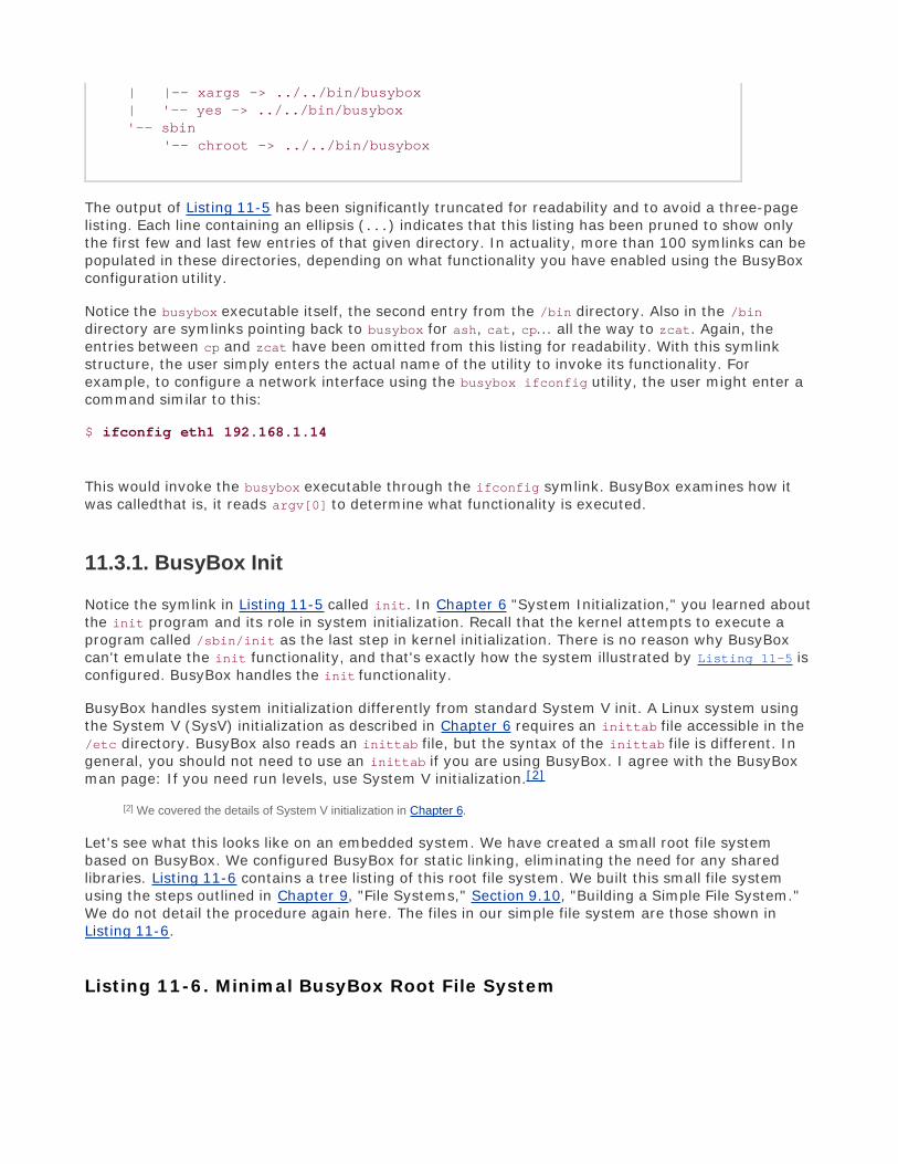
| |-- xargs -> ../../bin/busybox | '-- yes -> ../../bin/busybox '-- sbin '-- chroot -> ../../bin/busybox
The output of Listing 11-5 has been significantly truncated for readability and to avoid a three-pagelisting. Each line containing an ellipsis (...) indicates that this listing has been pruned to show onlythe first few and last few entries of that given directory. In actuality, more than 100 symlinks can bepopulated in these directories, depending on what functionality you have enabled using the BusyBoxconfiguration utility.
Notice the busybox executable itself, the second entry from the /bin directory. Also in the /bindirectory are symlinks pointing back to busybox for ash, cat, cp... all the way to zcat. Again, theentries between cp and zcat have been omitted from this listing for readability. With this symlinkstructure, the user simply enters the actual name of the utility to invoke its functionality. Forexample, to configure a network interface using the busybox ifconfig utility, the user might enter acommand similar to this:
$ ifconfig eth1 192.168.1.14
This would invoke the busybox executable through the ifconfig symlink. BusyBox examines how itwas calledthat is, it reads argv[0] to determine what functionality is executed.
11.3.1. BusyBox Init
Notice the symlink in Listing 11-5 called init. In Chapter 6 "System Initialization," you learned aboutthe init program and its role in system initialization. Recall that the kernel attempts to execute aprogram called /sbin/init as the last step in kernel initialization. There is no reason why BusyBoxcan't emulate the init functionality, and that's exactly how the system illustrated by Listing 11-5 isconfigured. BusyBox handles the init functionality.
BusyBox handles system initialization differently from standard System V init. A Linux system usingthe System V (SysV) initialization as described in Chapter 6 requires an inittab file accessible in the/etc directory. BusyBox also reads an inittab file, but the syntax of the inittab file is different. Ingeneral, you should not need to use an inittab if you are using BusyBox. I agree with the BusyBoxman page: If you need run levels, use System V initialization.[2]
[2] We covered the details of System V initialization in Chapter 6.
Let's see what this looks like on an embedded system. We have created a small root file systembased on BusyBox. We configured BusyBox for static linking, eliminating the need for any sharedlibraries. Listing 11-6 contains a tree listing of this root file system. We built this small file systemusing the steps outlined in Chapter 9, "File Systems," Section 9.10, "Building a Simple File System."We do not detail the procedure again here. The files in our simple file system are those shown inListing 11-6.
Listing 11-6. Minimal BusyBox Root File System

$ tree.|-- bin| |-- busybox| |-- cat -> busybox| |-- dmesg -> busybox| |-- echo -> busybox| |-- hostname -> busybox| |-- ls -> busybox| |-- ps -> busybox| |-- pwd -> busybox| '-- sh -> busybox|-- dev| '-- console|-- etc'-- proc4 directories, 10 files
This BusyBox-based root file system occupies little more than the size needed for busybox itself. Inthis configuration, using static linking and supporting nearly 100 utilities, the BusyBox executablecame in at less than 1MB:
# ls -l /bin/busybox-rwxr-xr-x 1 root root 824724 Dec 3 2005 /bin/busybox
Now let's see how this system behaves. Listing 11-7 captures the console output on power-up on thisBusyBox-based embedded system.
Listing 11-7. BusyBox Default Startup
...Looking up port of RPC 100003/2 on 192.168.1.9Looking up port of RPC 100005/1 on 192.168.1.9VFS: Mounted root (nfs filesystem).Freeing init memory: 96KBummer, could not run '/etc/init.d/rcS': No such file or directory
Please press Enter to activate this console.
BusyBox v1.01 (2005.12.03-19:09+0000) Built-in shell (ash)Enter 'help' for a list of built-in commands.
-sh: can't access tty; job control turned off/ #

The example of Listing 11-7 was run on an embedded board configured for NFS root mount. Weexport a directory on our workstation that contains the simple file system image detailed in Listing11-6. As oneof the final steps in the boot process, the Linux kernel on our target board mounts a rootfile system via NFS. When the kernel attempts to execute /sbin/init, it fails because there is no/sbin/init on our file system. However, as we have seen, the kernel also attempts to execute/bin/sh. In our BusyBox-configured target, this succeeds, and busybox is launched via the symlink/bin/sh on our root file system.
The first thing BusyBox displays is the complaint that it can't find /etc/init.d/rcS. This is the defaultinitialization script that BusyBox searches for. Instead of using inittab, this is the preferred methodto initialize an embedded system based on BusyBox.
When it has completed initialization, BusyBox displays a prompt asking the user to press Enter toactivate a console. When it detects the Enter key, it executes an ash shell session waiting for userinput. The final message about job control is a result of the fact that we are creating the systemconsole on a serial terminal. The Linux kernel contains code to disable job control if it detects theconsole on a serial terminal.
This example produced a working system, with nearly 100 Linux utilities available, including coreutilities, file utilities, network support, and a reasonably capable shell. You can see that this simplepackage provides a powerful platform upon which to build your own system applications. Of course, itshould be noted that without any support for libc and other system libraries, you would face aformidable task implementing your applications. You would have to provide support for all the usualsystem calls and other library functions that a typical C program relies on. Alternatively, you couldstatically link your applications against the libraries it depends on, but if you have more than a coupleapplications using this method, your applications will likely exceed the combined size of linkingdynamically and having the shared libraries on your target.
11.3.2. Example rcS Initialization Script
Before BusyBox spawns an interactive shell, it tries to execute commands from a script called/etc/init.d/rcS, as shown in Listing 11-7. It is here where your applications come to life in aBusyBox system. A simple rcS initialization script is provided in Listing 11-8.
Listing 11-8. Simple rcS BusyBox Startup Script

#!/bin/sh
echo "Mounting proc"mount -t proc /proc /proc
echo "Starting system loggers"syslogdklogd
echo "Configuring loopback interface"ifconfig lo 127.0.0.1
echo "Starting inetd"xinetd
# start a shellbusybox sh
This simple script is mostly self-explanatory. First, it is important to mount the /proc file system onits reserved mount point, /proc. This is because many utilities get their information from the /procfile system. This is explained more fully in Chapter 9. Next we launch the system loggers as early aspossible, to capture any startup problems. Following the system log daemons, we configure the localloopback interface for the system. Again, a number of traditional Linux facilities assume that aloopback interface is present, and if your system has support for sockets configured, you shouldenable this pseudo interface. The last thing we do before starting a shell is launch the Internetsuperserver xinetd. This program sits in the background listening for network requests on anyconfigured network interfaces. For example, to initiate a telnet session to the board, xinetdintercepts the request for telnet connection and spawns a telnet server to handle the session.
Instead of starting a shell, your own applications can be launched from this rcS initialization script.Listing 11-8 is a simple example of a Telnet-enabled target board running basic services such assystem and kernel loggers.
11.3.3. BusyBox Target Installation
The discussion of BusyBox installation can proceed only when you understand the use and purpose ofsymlinks. The BusyBox makefile contains a target called install. Executing make install creates adirectory structure containing the busybox executable and a symlink tree. This environment needs tobe migrated to your target embedded system's root directory, complete with the symlink tree. Thesymlink tree eliminates the need to type busybox command for each command. Instead, to see a listingof files in a given directory, the user need only type ls. The symlink executes busybox as describedpreviously and invokes the ls functionality. Review Listing 11-4 and Listing 11-5 to see the symlinktree. Note that the BusyBox build system creates links only for the functionality that you haveenabled via the configuration utility.
The easiest way to populate your root file system with the necessary symlink farm is to let theBusyBox build system do it for you. Simply mount your root file system on your developmentworkstation and pass a PREFIX to the BusyBox makefile. Listing 11-9 shows the procedure.

Listing 11-9. Installing BusyBox on Root File System
$ mount -o loop bbrootfs.ext2 /mnt/remote$ make PREFIX=/mnt/remote install/bin/sh applets/install.sh /mnt/remote /mnt/remote/bin/ash -> busybox /mnt/remote/bin/cat -> busybox /mnt/remote/bin/chgrp -> busybox /mnt/remote/bin/chmod -> busybox /mnt/remote/bin/chown -> busybox... /mnt/remote/usr/bin/xargs -> ../../bin/busybox /mnt/remote/usr/bin/yes -> ../../bin/busybox /mnt/remote/usr/sbin/chroot -> ../../bin/busybox
-------------------------------------------------- You will probably need to make your busybox binary setuid root to ensure all configured applets will work properly. --------------------------------------------------
$ chmod +s /mnt/remote/bin/busybox$ ls -l /mnt/remote/bin/busybox-rwsr-sr-x 1 root root 863188 Dec 4 15:54 /mnt/remote/bin/busybox
First we mount the root file system binary image on our desired mount pointin this case,/mnt/remote, a favorite of mine. Then we invoke the BusyBox make install command, passing it aPREFIX specifying where we want the symlink tree and busybox executable file to be placed. As youcan see from the listing, the makefile invokes a script called applets/install.sh to do the bulk of thework. The script walks through a file containing all the enabled BusyBox applets and creates asymlink for each one on the path we have specified using the PREFIX. The script is very chatty; itoutputs a line for each symlink created. For brevity, only the first few and last few symlinkannouncements are displayed. The ellipsis in the listing represents those we have eliminated.
The message about setuid is also displayed by the install script, to remind you that it might benecessary to make your busybox executable setuid root. This is to allow BusyBox functions thatrequire root access to function properly even when invoked by a nonroot user. This is not strictlynecessary, especially in an embedded Linux environment, where it is common to have only a rootaccount on a system. If this is necessary for your installation, the required command (chmod +s) isshown in Listing 11-9.
The result of this installation step is that the busybox binary and symlink tree are installed on ourtarget root file system. The end result looks very similar to Listing 11-4.
It is useful to note that BusyBox also has an option to enable creation of this symlink tree on thetarget system at runtime. This option is enabled in the BusyBox configuration and is invoked atruntime by executing busybox with the -install option. You must have the /proc file systemmounted on your target system for this support to work.

11.3.4. BusyBox Commands
In a recent BusyBox snapshot, 197 commands (also called applets) were documented in the manpage. There is sufficient support for reasonably complex shell scripts, including support for Bash shellscripting. BusyBox has support for awk and sed, frequently found in Bash scripts. BusyBox supportsnetwork utilities such as ping, ifconfig, TRaceroute, and netstat. Some commands are specificallyincluded for scripting support, including true, false, and yes.
Spend a few moments perusing Appendix C, "BusyBox Commands," where you can find a summaryof each BusyBox command. After you have done so, you will have a better appreciation for thecapabilities of BusyBox and how it might be applicable to your own embedded Linux project.
As mentioned at the beginning of this chapter, many of the BusyBox commands contain a limitedsubset of features and options compared to their full-featured counterparts. In general, you can gethelp on any given BusyBox command at runtime by invoking the command with the --help option.This produces a usage message with a brief description of each supported command option. TheBusyBox gzip applet is a useful example of a BusyBox command that has support for a limited set ofoptions. Listing 11-10 displays the output from gzip-help on a BusyBox target.
Listing 11-10. BusyBox gzip Applet Usage
/ # gzip --helpBusyBox v1.01 (2005.12.01-21:11+0000) multi-call binary
Usage: gzip [OPTION]... [FILE]...
Compress FILE(s) with maximum compression.When FILE is '-' or unspecified, reads standard input. Implies -c.
Options: -c Write output to standard output instead of FILE.gz -d Decompress -f Force write when destination is a terminal
The BusyBox version of gzip supports just three command line options. Its full-featured counterpartcontains support for more than 15 different command line options. For example, the full-featuredgzip utility supports a --list option that produces compression statistics for each file on thecommand line. No such support exists for BusyBox gzip. This is usually not a significant limitation forembedded systems. We present this information so you can make an informed choice when decidingon BusyBox. When the full capabilities of a utility are needed, the solution is simple: Delete supportfor that particular utility in the BusyBox configuration and add the standard Linux utility to yourtarget system.

11.4. Chapter Summary
BusyBox is a powerful tool for embedded systems that replaces many common Linux utilities ina single multicall binary.
BusyBox can significantly reduce the size of your root file system image.
BusyBox is easy to use and has many useful features.
Configuring BusyBox is straightforward, using an interface similar to that used for Linuxconfiguration.
BusyBox can be configured as a statically or dynamically linked application, depending on yourparticular requirements.
System initialization is somewhat different with BusyBox; those differences were covered in thischapter.
BusyBox has support for many commands. Appendix C itemizes all the available BusyBoxcommands from a recent release.
11.4.1. Suggestions for Additional Reading
BusyBox Project homewww.busybox.net/
BusyBox man pagewww.busybox.net/downloads/BusyBox.html

Chapter 12. Embedded DevelopmentEnvironmentIn this chapter
Cross-Development Environment page 290
Host System Requirements page 295
Hosting Target Boards page 296
Chapter Summary page 306
The configuration and services enabled on your host development system can have a huge impact onyour success as an embedded developer. This chapter examines the unique requirements of a cross-development environment and some of the tools and techniques that an embedded developer needsto know to be productive.
We begin by examining a typical cross-development environment. Using the familiar "hello world"example, we detail the important differences between host-based applications and those targeted atembedded systems. We also look at differences in the toolchains for native versus embeddedapplication development. We then present host system requirements and detail the use of someimportant elements of your host system. We conclude this chapter with an example of a target boardbeing hosted by a network-based host.

12.1. Cross-Development Environment
Developers new to embedded development often struggle with the concepts and differences betweennative and cross-development environments. Indeed, there are often three compilers and three (ormore) versions of standard header files such as stdlib.h . Debugging an application on your targetembedded system can be difficult without the right tools and host-based utilities. You must manageand separate the files and utilities designed to run on your host system from those you intend to useon your target.
When we use the term host in this context, we are referring to the development workstation that issitting on your desktop and running your favorite Linux desktop distribution.[1] Conversely, when weuse the term target we are referring to your embedded hardware platform. Therefore, nativedevelopment denotes the compilation and building of applications on and for your host system.Cross-development denotes the compilation and building of applications on the host system that willbe run on the embedded system. Keeping these definitions in mind will help you stay on trackthrough this chapter.
[1] Webster's defines nonsense as "an idea that is absurd or contrary to good sense." It is my opinion that developing embedded
Linux platforms on a non-Linux/UNIX host is nonsensical.
Figure 12-1 shows the layout of a typical cross-development environment. A host PC is connected toa target board via one or more physical connections. It is most convenient if both serial and Ethernetports are available on the target. Later when we discuss kernel debugging, you will realize that asecond serial port can be a very valuable asset.
Figure 12-1. Cross-development setup
In the most common scenario, the developer has a serial terminal on the host connected to the RS-232 serial port, possibly one or more Telnet terminal sessions to the target board, and potentially oneor more debug sessions using Ethernet as the connection medium. This cross-development setupprovides a great deal of flexibility. The basic idea is that the host system provides the horsepower to

run the compilers, debuggers, editors, and other utilities, while the target executes only theapplications designed for it. Yes, you can certainly run compilers and debuggers on the targetsystem, but we assume that your host system contains more resources, including RAM, disk storage,and Internet connectivity. In fact, it is not uncommon for a target embedded board to have nohuman-input devices or output displays.
12.1.1. "Hello World"Embedded
A properly configured cross-development system hides a great deal of complexity from the averageapplication developer. Looking at a simple example will help uncover and explain some of themystery. When we compile a simple "hello world" program, the toolchain (compiler, linker, andassociated utilities) makes many assumptions about the host system we are building on and theprogram we are compiling. Actually, they are not assumptions, but a collection of rules that thecompiler references to build a proper binary.
Listing 12-1 reproduces a simple "hello world" program.
Listing 12-1. Hello World Again
#include <stdio.h>
int main(int argc, char **argv){ printf("Hello World\n"); return 0;}
Even the casual application developer will realize some important points about this C source file. First,the function printf() is referenced but not defined in this file. If we omit the #include directivecontaining the prototype for the printf() function, the compiler emits the familiar message:
hello.c:5: warning: implicit declaration of function 'printf'
This introduces some interesting questions:
Where is the file stdio.h located, and how is it found?
Where does the printf() function live, and how is this reference resolved in the binaryexecutable?
Somehow it seems that the compiler just knows how to put together a proper binary file that isexecutable from the command line. To further complicate matters, the final executable containsstartup and shutdown prologue code that we never see but that the linker automatically includes.This prologue deals with details such as the environment and arguments passed to your program,startup and shutdown housekeeping, exit handling, and more.
To build the "hello world" application, we can use a simple command line invocation of the compiler,similar to this:

$ gcc -o hello hello.c
This produces the binary executable file called hello , which we can execute directly from thecommand line. Defaults referenced by the compiler provide guidance on where include files will befound. In a similar fashion, the linker knows how to resolve the reference to the printf() function byincluding a reference to the library where it is defined. This, of course, is the standard C library.
We can query the toolchain to see some of the defaults that were used. Listing 12-2 is a partial listingof the output from cpp when passed the -v flag. You might already know that cpp is the Cpreprocessor component of the gcc toolchain. We have added some formatting (whitespace only) toimprove the readability.
Listing 12-2. Default Native cpp Search Directories
[View full width]
$ cpp -vReading specs from /usr/lib/gcc-lib/i386-redhat-linux/3.3.3/specsConfigured with: ../configure --prefix=/usr --mandir=/usr/share/man --infodir=/usr/share/info --enable-shared --enable-threads=posix --disable-checking --disable-libunwind-exceptions --with-system-zlib --enable-__cxa_atexit -host=i386-redhat-linux
Thread model: posixgcc version 3.3.3 20040412 (Red Hat Linux 3.3.3-7) /usr/lib/gcc-lib/i386-redhat-linux/3.3.3/cc1 -E -quiet -v -ignoring nonexistent directory "/usr/i386-redhat-linux/include"
#include "..." search starts here:#include <...> search starts here: /usr/local/include /usr/lib/gcc-lib/i386-redhat-linux/3.3.3/include /usr/includeEnd of search list./usr/lib/
This simple query produces some very useful information. First, we can see how the compiler wasconfigured using the familiar ./configure utility. The default thread model is posix , whichdetermines the thread library your application gets linked against if you employ threading functions.Finally, you see the default search directories for #include directives.
But what if we want to build hello.c for a different architecture, such as PowerPC? When we compilean application program for a PowerPC target using a cross-compiler on our host machine, we mustmake sure that the compiler does not use the default host include directories or library paths. Usinga properly configured cross-compiler is the first step, and having a well designed cross-developmentenvironment is the second.
Listing 12-3 is the output from a popular open-source cross-development toolchain known as theEmbedded Linux Development Kit (ELDK), assembled and maintained by Denx Software Engineering.This particular installation was configured for the PowerPC 82xx toolchain. Again, we have added

some whitespace to the output for readability.
Listing 12-3. Default Cross-Search Directories
[View full width]
$ ppc_82xx-cpp -vReading specs from /opt/eldk/usr/bin/.. /lib/gcc-lib/ppc-linux/3.3.3/specs
Configured with: ../configure --prefix=/usr --mandir=/usr/share/man --infodir=/usr/share/info --enable-shared --enable-threads=posix --disable-checking --with-system-zlib --enable-__cxa_atexit --with-newlib --enable-languages=c,c++ --disable-libgcj --host=i386-redhat-linux -target=ppc-linux
Thread model: posix
gcc version 3.3.3 (DENX ELDK 3.1.1 3.3.3-10) /opt/eldk/usr/bin/../lib/gcc-lib/ppc-linux/3.3.3/cc1 -E -quiet -v -iprefix /opt/eldk/usr/bin/.. /lib/gcc-lib/ppc-linux/3.3.3/ -D__unix__ -D__gnu_linux__ -D__linux__ -Dunix -D__unix -Dlinux -D__linux -Asystem=unix -Asystem=posix - -mcpu=603
ignoring nonexistent directory "/opt/eldk/usr/ppc-linux/sys-include"ignoring nonexistent directory "/opt/eldk/usr/ppc-linux/include"#include "..." search starts here:
#include <...> search starts here: /opt/eldk/usr/lib/gcc-lib/ppc-linux/3.3.3/include /opt/eldk/ppc_82xx/usr/include
End of search list.
Here you can see that the default search paths for include directories are now adjusted to point toyour cross versions instead of the native include directories. This seemingly obscure detail is criticalto being able to develop applications and compile open-source packages for your embedded system.It is one of the most confusing topics to even experienced application developers who are new toembedded systems.

12.2. Host System Requirements
Your development workstation must include several important components and systems. Of course,you need a properly configured cross toolchain. You can download and compile one yourself or obtainone of the many commercial toolchains available. Building one yourself is beyond the scope of thisbook, although there are several good references available. See Section 12.4.1, "Suggestions forAdditional Reading," at the end of this chapter for recommendations.
The next major item you need is a Linux distribution targeted for your embedded systemarchitecture. This includes hundreds to potentially thousands of files that will populate yourembedded system's file systems. Again, the choices are to build your own or to obtain one of thecommercial ones. One of the more popular embedded system distributions available on the Internetis the aforementioned ELDK. The ELDK is available for some PowerPC and other embedded targets.Building an embedded Linux distribution from scratch would require a book of this size in itself and,therefore, is beyond the scope of our discussions here.
In summary, your development host requires four separate and distinct capabilities:
Cross toolchain and libraries
Target system packages, including programs, utilities, and libraries
Host tools such as editors, debuggers, and utilities
Servers for hosting your target board, covered in the next section
If you install a ready-built embedded Linux development environment on your workstation, either acommercial variety or one freely available in the open source community, the toolchain andcomponents have already been preconfigured to work together. For example, the toolchain has beenconfigured with default directory search paths that match the location of the target header files andsystem libraries on your development workstation. The situation becomes much more complex if yourrequirements include having support for multiple architectures and processors on your developmentworkstation. This is the reason that embedded Linux distributions exist.
12.2.1. Hardware Debug Probe
In addition to the components listed previously, you should consider some type of hardware-assisteddebugging. This consists of a hardware probe connected to your host (often via Ethernet) andconnected to your target via a debug connector on the board. Many solutions are on the markettoday. We cover this topic in detail in Chapter 14, "Kernel Debugging Techniques."

12.3. Hosting Target Boards
Referring back to Figure 12-1 , you will notice an Ethernet connection from the target-embeddedboard to the host-development system. This is not strictly necessary, and, indeed, some smallerembedded devices do not have an Ethernet interface. However, this is the exception rather than therule. Having an Ethernet connection available on your target board is worth its cost in silicon!
While developing the kernel, you will compile and download kernels to your embedded board manytimes. Many embedded development systems and bootloaders have support for TFTP and assumethat the developer will use it. TFTP is a lightweight protocol for moving files between a TFTP serverand TFTP client, similar to FTP.
Using TFTP from your bootloader to load the kernel will save you countless hours waiting for serialdownloads even at higher serial baud rates. And loading your ramdisk can take much longer becauseramdisk images can grow to many tens of megabytes and more, depending on your requirements.The investment in your time to configure and use TFTP will surely pay off and is highly recommended.There are very few designs that can't afford the real estate to include an Ethernet port duringdevelopment, even if it is depopulated for production.
12.3.1. TFTP Server
Configuring TFTP on your Linux development host is not difficult. Of course, the details might vary,depending on which Linux distribution you choose for your development workstation. The guidelinespresented here are based on Red Hat and Fedora Core Linux distributions.
TFTP is a TCP/IP service that must be enabled on your workstation. To enable TFTP service, you mustinstruct your server to respond to incoming TFTP packets and spawn your TFTP server. On manyLinux distributions, this is done by editing a configuration file used by the xinetd Internetsuperserver. For example, on the Red Hat and Fedora desktop Linux distributions, this file is/etc/xinetd.d/tftp . Listing 12-4 contains a TFTP configuration from a Fedora Core 2 developmentworkstation to enable the TFTP service. It has been slightly rearranged to fit the page.
Listing 12-4. TFTP Configuration
# default: off # description: The tftp server serves files using the trivial # file transfer protocol. The tftp protocol is often used to # boot diskless workstations, download configuration files to # network-aware printers, and to start the installation process # for some operating systems.
service tftp { socket_type = dgram

protocol = udp wait = yes user = root server = /usr/sbin/in.tftpd server_args = -c -s /tftpboot disable = no per_source = 11 cps = 100 2 flags = IPv4 }
In this typical setup, the TFTP service has been enabled (disable = no ) and configured to serve fileslocated in this workstation's /tftpboot directory. When the xinetd Internet superserver receives anincoming TFTP request, it consults this configuration and spawns the server specified(/usr/sbin/in.tftpd ). The command line arguments specified by server_args are passed to thein.tftpd process. In this case, the -s switch tells in.tftpd to switch to the specified directory(/tftpboot ), and the -c flag allows the creation of new files. This is useful to write files to the serverfrom the target.
Consult the documentation that came with your desktop distribution for details specific to yourenvironment.
12.3.2. BOOTP/DHCP Server
Having a DHCP server on your development host simplifies the configuration management for yourembedded target. We have already established the reasons why an Ethernet interface on your targethardware is a good idea. When Linux boots on your target board, it needs to configure the Ethernetinterface before the interface will be useful. Moreover, if you are using an NFS root mountconfiguration on your target board, Linux needs to configure your target's Ethernet interface beforethe boot process can complete. We covered NFS in detail in Chapter 9 , "File Systems."
In general, Linux can use two methods to initialize its Ethernet/IP interface during boot:
Hard-code the Ethernet interface parameters either on the Linux kernel command line or in thedefault configuration
Configure the kernel to automatically detect the network settings at boot time
For obvious reasons, the latter choice is the most flexible. DHCP or BOOTP is the protocol your targetand server use to accomplish the automatic detection of network settings. For details of the DHCP orBOOTP protocols, see Section 12.4.1 at the end of this chapter.
A DHCP server controls the IP address assignments for IP subnets for which it has been configured,and for DHCP or BOOTP clients that have been configured to participate. A DHCP server listens forrequests from a DHCP client (such as your target board), and assigns addresses and other pertinentinformation to the client as part of the boot process. A typical DHCP exchange (see Listing 12-5 ) canbe examined by starting your DHCP server with the -d debug switch and observing the output when atarget machine requests configuration.

Listing 12-5. Typical DHCP Exchange
tgt> DHCPDISCOVER from 00:09:5b:65:1d:d5 via eth0 svr> DHCPOFFER on 192.168.0.9 to 00:09:5b:65:1d:d5 via eth0 tgt> DHCPREQUEST for 192.168.0.9 (192.168.0.1) from \ 00:09:5b:65:1d:d5 via eth0 svr> DHCPACK on 192.168.0.9 to 00:09:5b:65:1d:d5 via eth0
The sequence starts with the client (target) transmitting a broadcast frame attempting to discover aDHCP server. This is shown by the DHCPDISCOVER message shown. The server responds (if it has beenso configured and enabled) by offering an IP address for the client. This is evidenced by theDHCPOFFER message. The client then responds by testing this IP address locally. The testing includessending the DHCPREQUEST packet to the DHCP server, as shown. Finally, the server responds byacknowledging the IP address assignment to the client, thus completing the automatic targetconfiguration.
It is interesting to note that a properly configured client will remember the last address it wasassigned by a DHCP server. The next time it boots, it will skip the DHCPDISCOVER stage and proceeddirectly to the DHCPREQUEST stage, assuming that it can reuse the same IP address that the serverpreviously assigned. A booting Linux kernel does not have this capability and emits the samesequence every time it boots.
Configuration of your host's DHCP server is not difficult. As usual, our advice is to consult thedocumentation that came with your desktop Linux distribution. On a Red Hat or Fedora Coredistribution, the configuration entry for a single target might look like Listing 12-6 .
Listing 12-6. Example DHCP Server Configuration
# Example DHCP Server configuration allow bootp;
subnet 192.168.1.0 netmask 255.255.255.0 { default-lease-time 1209600; # two weeks option routers 192.168.1.1; option domain-name-servers 1.2.3.4; group { host pdna1 { hardware ethernet 00:30:bd:2a:26:1f; fixed-address 192.168.1.68; filename "uImage-pdna"; option root-path "/home/chris/sandbox/pdna-target"; } } }
This is a simple example, meant only to show the kind of information you can pass to your targetsystem. There is a one-to-one mapping of the target MAC address to its assigned IP address. Inaddition to its fixed IP address, you can pass other information to your target. In this example, thedefault router and DNS server addresses are passed to your target, along with the filename of a file

of your choice, and a root path for your kernel to mount an NFS root mount from. The filename mightbe used by your bootloader to load a kernel image from your TFTP server. You can also configureyour DHCP server to hand out IP addresses from a predefined range, but it is very convenient to usea fixed address such as that shown in Listing 12-6 .
You must enable the DHCP server on your Linux development workstation. This is typically donethrough your main menu or via the command line. Consult the documentation for your own Linuxdistribution for details suitable for your environment. For example, to enable the DHCP server on aFedora Core 2 Linux distribution, simply type the following command from a root command prompt:
$ /etc/init.d/dhcpd start (or restart)
You must do this each time you start your development workstation, unless you configure it to startautomatically.
Many nuances are involved with installing a DHCP server, so unless your server is on a privatenetwork, it is advisable to check with your system administrator before going live with your own. Ifyou coexist with a corporate LAN, it is very possible that you will interfere with its own DHCP service.
12.3.3. NFS Server
Using an NFS root mount for your target board is a very powerful development tool. Some of theadvantages of this configuration for development are:
Your root file system is not size-restricted by your board's own limited resources, such as Flashmemory.
Changes made to your application files during development are immediately available to yourtarget system.
You can debug and boot your kernel before developing and debugging your root file system.
Setting up an NFS server varies depending on the desktop Linux distribution you are using. As withthe other services described in this chapter, you must consult the documentation for your own Linuxdistribution for the details appropriate to your configuration. The NFS service must be started fromeither your startup scripts, a graphical menu, or the command line. For example, the command tostart NFS services from a root command prompt for a Fedora Core 2 Linux desktop is as follows:
$ /etc/init.d/nfs start (or restart)
You must do this each time you start your desktop Linux workstation. (This and other services can bestarted automatically on bootingconsult the documentation for your desktop Linux distribution.) Inaddition to enabling the service, your kernel must be compiled with support for NFS. Although DHCPand TFTP are both user space utilities, NFS requires kernel support. This is true on both yourdevelopment workstation and your target board. Figure 12-2 illustrates the configuration options forNFS in the kernel. Notice that there are configuration options for both NFS server and client support.Note also the option for root file system on NFS. Your target kernel must have this option configuredfor NFS root mount operation.

Figure 12-2. NFS kernel configuration
[View full size image]
The NFS server gets its instructions from an exports file located on your server. It is commonly foundin /etc/exports . Listing 12-7 is an example of a simple exports entry.
Listing 12-7. Simple NFS exports File
$ cat /etc/exports # /etc/exports /home/chris/sandbox/coyote-target *(rw,sync,no_root_squash) /home/chris/sandbox/pdna-target *(rw,sync,no_root_squash) /home/chris/workspace *(rw,sync,no_root_squash)
These entries on my workstation allow a client to remotely mount any of the three directories shown.The attributes following the directory specification instruct the NFS server to allow connections fromany IP address (*) and to mount the respective directories with the given attributes (read/write withno_root_squash ). The latter attribute enables a client with root privileges to exercise those privilegeson the given directory. It is usually required when working with embedded systems because theyoften have only root accounts.
You can test your NFS configuration right from your workstation. Assuming that you have NFSservices enabled (requires both NFS server and client components enabled), you can mount a localNFS export as you would mount any other file system:
# mount -t nfs localhost:/home/chris/workspace /mnt/remote

If this command succeeds and the files in .../workspace are available on /mnt/remote , your NFSserver configuration is working.
12.3.4. Target NFS Root Mount
Mounting your target via NFS root mount is not difficult, and, as mentioned elsewhere, it is a veryuseful development configuration. However, a set of details must be correct before it will work. Thesteps required are as follows:
Configure your NFS server and export a proper target file system for your architecture.1.
Configure your target kernel with NFS client services and root file system on NFS.2.
Enable kernel-level autoconfiguration of your target's Ethernet interface.3.
Provide your target Ethernet IP configuration via the kernel command line or static kernelconfiguration option.
4.
Provide a kernel command line enabled for NFS.5.
We presented the kernel configuration in Figure 12-2 when we explained the NFS serverconfiguration. You must make sure that your target kernel configuration has NFS client servicesenabled, and, in particular, you must enable the option for Root file system on NFS. Specifically,make sure that your kernel has CONFIG_NFS_FS=y and CONFIG_ROOT_NFS=y . Obviously, you cannotconfigure NFS as loadable modules if you intend to boot NFS root mount.
Kernel-level autoconfiguration is a TCP/IP configuration option found under the Networking tab in thekernel configuration utility. Enable CONFIG_IP_PNP on your target kernel. When selected, you arepresented with several options for automatic configuration. Select either BOOTP or DHCP, asdescribed earlier. Figure 12-3 illustrates the kernel configuration for kernel-level autoconfiguration.
Figure 12-3. Kernel-level autoconfiguration
[View full size image]

When your server and target kernel are configured, you need to provide your target Ethernetconfiguration via one of the methods described earlier. If your bootloader supports a kernel commandline, that is the easiest method. Here is what a kernel command line might look like to support NFSroot mount:
console=ttyS0,115200 root=/dev/nfs rw ip=dhcp \ nfsroot=192.168.1.9:/home/chris/sandbox/pdna-target
12.3.5. U-Boot NFS Root Mount Example
U-Boot is a good example of a bootloader that supports a configurable kernel command line. Using U-Boot's nonvolatile environment feature, we can store our kernel command line in a parameterspecially named for this purpose. To enable the NFS command line in U-Boot, we do the following (allon one line in our serial terminal):
setenv bootargs console=ttyS0,115200 root=/dev/nfs rw \ ip=dhcp nfsroot=192.168.1.9:/home/chris/sandbox/pdna-target
Then we load a kernel via our TFTP server. Listing 12-8 shows what this might look like on a PowerPCembedded target.
Listing 12-8. Loading Kernel via TFTP Server
=> tftpboot 200000 uImage-pdna <<< Entered at U-Boot prompt Using FEC ETHERNET device TFTP from server 192.168.1.9; our IP address is 192.168.1.68

Filename 'uImage-pdna'. Load address: 0x200000 Loading: ################################################## ################################################## ######################################### done Bytes transferred = 911984 (dea70 hex) =>
When we boot the kernel, we see specific evidence of our NFS root mount configuration. Listing 12-9reproduces selected output from the kernel boot messages to demonstrate this. This output has beenformatted (many lines omitted and whitespace added) for readability.
Listing 12-9. Booting with NFS Root Mount
[View full width]
Uncompressing Kernel Image ... OK Linux version 2.6.14 (chris@pluto) (gcc version 3.3.3 (DENX ELDK 3.1.1 3.3.3-10)) #1 Mon Jan 2 11:58:48 EST 2006 . . Kernel command line: console=ttyS0,115200 root=/dev/nfs rw nfsroot=192.168.1.9:/home/chris/sandbox/pdna-target ip=dhcp . . Sending DHCP requests ... OK IP-Config: Got DHCP answer from 192.168.1.9, my address is 192.168.1.68 IP-Config: Complete: device=eth0, addr=192.168.1.68, mask=255.255.255.0, gw=255.255.255.255, host=192.168.1.68, domain=, nis-domain=(none), bootserver=192.168.1.9, rootserver=192.168.1.9, rootpath=/home/chris/sandbox/pdna-target . . Looking up port of RPC 100003/2 on 192.168.1.9 Looking up port of RPC 100005/1 on 192.168.1.9 VFS: Mounted root (nfs filesystem). . .
BusyBox v0.60.5 (2005.06.07-07:03+0000) Built-in shell (msh) Enter 'help' for a list of built-in commands.
#
From Listing 12-9 , first we see the kernel banner followed by the kernel command line. We specified

four items in this kernel command line:
Console device (/dev/console )
Root device (/dev/nfs )
NFS root path (/home/chris/sandbox/pdna-target )
IP kernel-level autoconfiguration method (dhcp )
Shortly thereafter, we see the kernel attempting kernel-level autoconfiguration via DHCP. When theserver responds and the DHCP exchange completes, the kernel displays the detected configuration inthe following lines. You can see from this listing that the DHCP server has assigned the target the IPaddress 192.168.1.68. Compare the detected settings with those specified in Listing 12-6 . That wassimilar to the DHCP server configuration that resulted in this configuration.
When the kernel has completed the IP autoconfiguration, it is capable of mounting the root filesystem using the supplied parameters. You can see this from the three lines ending with the VFS(virtual file subsystem) message announcing that it has mounted the root NFS file system. After theNFS root file system has been mounted, initialization completes as described in Chapter 5 , "KernelInitialization."
It is also possible to pass target IP settings to the kernel in a static fashion instead of having thekernel obtain IP settings from a DHCP or BOOTP server. IP settings can be passed via the kernelcommand line directly. In this case, the kernel command line might look similar to this:
[View full width]console=console=ttyS0,115200 \ ip=192.168.1.68:192.168.1.9::255.255.255.0:pdna:eth0:off \ root=/dev/nfs rw nfsroot=192.168.1.9:/home/chris/pdna-target

12.4. Chapter Summary
Many features of a development environment greatly facilitate efficiency for embedded cross-development. Most of these fall under the category of tools and utilities. We cover this aspect indetail in the next chapter, where we cover development tools.
A properly configured development host is a critical asset for the embedded developer.
Toolchains employed for cross-development must be properly configured to match your hostsystem's target Linux environment.
Your development host must have target components installed that your toolchain and binaryutilities can reference. These components include target header files, libraries, target binaries,and their associated configuration files. In short, you need to assemble or obtain an embeddedLinux distribution.
Configuring target servers such as TFTP, DHCP, and NFS will greatly increase your productivityas an embedded Linux developer. This chapter introduced configuration examples for each.
12.4.1. Suggestions for Additional Reading
GCC online documentationhttp://gcc.gnu.org/onlinedocs/
Building and testing gcc/glibc cross toolchainshttp://kegel.com/crosstool/
The TFTP Protocol, Version 2RFC 1350www.ietf.org/rfc/rfc1350.txt?number=1350
Bootstrap Protocol (BOOTP)RFC 951www.ietf.org/rfc/rfc0951.txt?number=951
Dynamic Host Configuration ProtocolRFC 2131www.ietf.org/rfc/rfc2131.txt?number=2131

Chapter 13. Development ToolsIn this chapter
GNU Debugger (GDB) page 310
Data Display Debugger page 317
cbrowser/cscope page 319
Tracing and Profiling Tools page 321
Binary Utilities page 340
Miscellaneous Binary Utilities page 346
Chapter Summary page 349
A typical embedded Linux distribution includes many useful tools. Some are complex and require agreat deal of proficiency to master. Others are simple and have been all but ignored by developers ofembedded systems. Some tools might require customization for a particular environment. Many willrun "right out of the box" and provide the developer with useful information without much effort. Thischapter presents a cross-section of the most important (and frequently neglected) tools available tothe embedded Linux engineer.
It is impossible to provide complete details on the tools and utilities presented in this chapter. Thatwould take an entire book by itself! Rather than provide a complete reference, our goal is to providean introduction on the basic usage of each one. You are encouraged to pursue additional study onthese and other important development tools. The man page (or other documentation) for each toolis a great place to start.
The GNU Debugger (GDB) is introduced first, followed by a brief look at the Data Display Debugger, agraphical front end for GDB. Next we introduce a series of utilities designed to give the developer alook at the behavior of programs and the system as a whole. These include strace, ltrace, top,and ps, often overlooked by inexperienced Linux developers. We then present some crash dump andmemory-analysis tools. The chapter concludes by introducing some of the more useful binary utilities.

13.1. GNU Debugger (GDB)
If you spend much time developing Linux applications, you will undoubtedly spend many hoursgetting to know the GNU Debugger. GDB is arguably the most important tool in the developer'stoolbox. It has a long history, and its capabilities have blossomed to include low-level hardware-specific debugging support for a wide variety of architectures and microprocessors. It should be notedthat the user manual for GDB is nearly as large as this book. Our intention here is to introduce GDBto get you started. You are encouraged to study the user manual referenced later under Section13.7.1 , "Suggestions for Additional Reading."
Because this is a book about embedded Linux development, we use a version of GDB that has beencompiled as a cross-debugger. That is, the debugger itself runs on your development host, but itunderstands binary executables in the architecture for which it was configured at compile time. In thenext few examples, we use GDB compiled for a Red Hat Linux-compatible development host, and anXScale (ARM) target processor. Although we use the short name gdb , we are presenting examplesbased on the XScale-enabled cross-gdb from the Monta Vista embedded Linux distribution for ARMXScale. The binary is called xscale_be-gdb . It is still GDB, simply configured for a cross-developmentenvironment.
The GDB debugger is a complex program with many configuration options during the build process. Itis not our intention to provide guidance on building gdb that has been covered in other literature. Forthe purposes of this chapter, we assume that you have obtained a working GDB configured for thearchitecture and host development environment you will be using.
13.1.1. Debugging a Core Dump
One of the most common reasons to drag GDB out of the toolbox is to evaluate a core dump . It isquick and easy, and often leads to immediate identification of the offending code. A core dumpresults when an application program generates a fault, such as accessing a memory location that itdoes not own. Many conditions can trigger a core dump,[1] but SIGSEGV (segmentation fault) is byfar the most common. A SIGSEGV is a Linux kernel signal that is generated on illegal memoryaccesses by a user process. When this signal is generated, the kernel terminates the process. Thekernel then dumps a core image, if so enabled.
[1] See SIG_KERNEL_COREDUMP_MASK in .../kernel/signal.c for a definition of which signals generate a core dump.
To enable generation of a core dump, your process must have the resource limits to enable a coredump. This is achieved by setting the process's resource limits using the setrlimit() function call, orfrom a BASH or BusyBox shell command prompt, using ulimit . It is not uncommon to find thefollowing line in the initialization scripts of an embedded system to enable the generation of coredumps on process errors:
$ ulimit -c unlimited

This BASH built-in command is used to set the size limit of a core dump. In the previous instance, thesize is set to unlimited.
When an application program generates a segmentation fault (for example, by writing to a memoryaddress outside its permissible range), Linux terminates the process and generates a core dump, ifso enabled. The core dump is a snapshot of the running process at the time the segmentation faultoccurred.
It helps to have debugging symbols enabled in your binary. GDB produces much more useful outputwith debugging symbols (gcc -g ) enabled during the build. However, it is still possible to determinethe sequence of events leading to the segmentation fault, even if the binary was compiled withoutdebugging symbols. You might need to do a bit more investigative work without the aid of debuggingsymbols. You must manually correlate virtual addresses to locations within your program.
Listing 13-1 shows the results of a core dump analysis session using GDB. The output has beenreformatted slightly to fit the page. We have used some demonstration software to intentionallyproduce a segmentation fault. Here is the output of the process (called webs ) that generated thesegmentation fault:
root@coyote:/workspace/websdemo# ./webs Segmentation fault (core dumped)
Listing 13-1. Core Dump Analysis Using GDB
$ xscale_be-gdb webs coreGNU gdb 6.3 (MontaVista 6.3-20.0.22.0501131 2005-07-23)Copyright 2004 Free Software Foundation, Inc.GDB is free software, covered by the GNU General PublicLicense, and you are welcome to change it and/or distribute cop-ies of it under certain conditions.Type "show copying" to see the conditions.There is absolutely no warranty for GDB. Type "show warranty"for details.This GDB was configured as "--host=i686-pc-linux-gnu -target=armv5teb-montavista-linuxeabi"...
Core was generated by './webs'.Program terminated with signal 11, Segmentation fault.Reading symbols from /opt/montavista/pro/.../libc.so.6...done.Loaded symbols for /opt/montavista/pro/.../libc.so.6Reading symbols from /opt/montavista/pro/.../ld-linux.so.3...done.Loaded symbols for /opt/montavista/pro/.../ld-linux.so.3#0 0x00012ac4 in ClearBlock (RealBigBlockPtr=0x0, l=100000000) at led.c:4343 *ptr = 0;
(gdb) l3839 static int ClearBlock(char * BlockPtr, int l)40 {41 char * ptr;42 for (ptr = BlockPtr; (ptr - BlockPtr) < l; ptr++)

43 *ptr = 0;44 return 0;45 }46 static int InitBlock(char * ptr, int n)47 {(gdb) p ptr$1 = 0x0(gdb)
13.1.2. Invoking GDB
The first line of Listing 13-1 shows how GDB was invoked from the command line. Because we aredoing cross-debugging, we need the cross-version of GDB that has been compiled for our host andtarget system. We invoke our version of cross-gdb as shown and pass xscale_be-gdb the name of thebinary followed by the name of the core dump filein this case, simply core . After GDB prints severalbanner lines describing its configuration and other information, it prints the reason for thetermination: signal 11, the indication of a segmentation fault.[2] Several lines follow as GDB loads thebinary, the libraries it depends on, and the core file. The last line printed upon GDB startup is thecurrent location of the program when the fault occurred. The line preceded by the #0 string indicatesthe stack frame (stack frame zero in a function called ClearBlock() at virtual address 0x00012ac4).The following line preceded by 43 is the line number of the offending source line from a file calledled.c . From there, GDB displays its command prompt and waits for input.
[2] Signals and their associated numbers are defined in .../asm-<arch>/signal.h in your Linux kernel source tree.
To provide some context, we enter the gdb list command, using its abbreviated form l . GDBrecognizes command abbreviations where there is no ambiguity. Here the program error begins topresent itself. The offending line, according to GDB's analysis of the core dump is:
43 *ptr = 0;
Next we issue the gdb print command on the ptr variable, again abbreviated as p . As you can seefrom Listing 13-1 , the value of the pointer ptr is 0 . So we conclude that the reason for thesegmentation fault is the dereference of a null pointer, a common programming error. From here, wecan elect to use the backtrace command to see the call chain leading to this error, which might leadus back to the actual source of the error. Listing 13-2 displays these results.
Listing 13-2. Backtrace Command
(gdb) bt#0 0x00012ac4 in ClearBlock (RealBigBlockPtr=0x0, l=100000000) at led.c:43#1 0x00012b08 in InitBlock (ptr=0x0, n=100000000) at led.c:48#2 0x00012b50 in ErrorInHandler (wp=0x325c8, urlPrefix=0x2f648 "/Error", webDir=0x2f660 "", arg=0, url=0x34f30 "/Error", path=0x34d68 "/Error", query=0x321d8 "") at led.c:61#3 0x000126cc in websUrlHandlerRequest (wp=0x325c8) at handler.c:273#4 0x0001f518 in websGetInput (wp=0x325c8, ptext=0xbefffc40, pnbytes=0xbefffc38) at webs.c:664#5 0x0001ede0 in websReadEvent (wp=0x325c8) at webs.c:362

#6 0x0001ed34 in websSocketEvent (sid=1, mask=2, iwp=206280) at webs.c:319#7 0x00019740 in socketDoEvent (sp=0x34fc8) at sockGen.c:903#8 0x00019598 in socketProcess (sid=1) at sockGen.c:845#9 0x00012be8 in main (argc=1, argv=0xbefffe14) at main.c:99(gdb)
The backtrace displays the call chain all the way back to main() , the start of the user's program. Astack frame number precedes each line of the backtrace. You can switch to any given stack frameusing the gdb frame command. Listing 13-3 is an example of this. Here we switch to stack frame 2and display the source code in that frame. As in the previous examples, the lines preceded with (gdb) are the commands we issue to GDB, and the other lines are the GDB output.
Listing 13-3. Moving Around Stack Frames in GDB
(gdb) frame 2#2 0x00012b50 in ErrorInHandler (wp=0x325c8, urlPrefix=0x2f648 "/Error", webDir=0x2f660 "", arg=0, url=0x34f30 "/Error", path=0x34d68 "/Error", query=0x321d8 "") at led.c:6161 return InitBlock(p, siz);(gdb) l5657 siz = 10000 * sizeof(BigBlock);5859 p = malloc(siz);60 /* if (p) */61 return InitBlock(p, siz);62 /* else return (0); */63 }6465(gdb)
As you can see, with a little help from the source code available using the list command, it wouldnot be difficult to trace the code back to the source of the errant null pointer. In fact, the astutereader will notice the source of the segmentation fault we have produced for this example. FromListing 13-3 , we see that the check of the return value in the call to malloc() has been commentedout. In this example, the malloc() call failed, leading to the operation on a null pointer two frameslater in the call chain. Although this example is both contrived and trivial, many crashes of this typeare remarkably easy to track down using a similar method with GDB and core dumps. You can alsosee the null pointer by looking at the parameter values in the function call. This often leads youdirectly to the frame where the null pointer originated.
13.1.3. Debug Session in GDB
We conclude this introduction to GDB by showing a typical debug session. In the previousdemonstration of a program crash, we could have elected to step through the code to narrow downthe cause of the failure. Of course, if you get a core dump, you should always start there. However,in other situations, you might want to set breakpoints and step through running code. Listing 13-4

details how we start GDB in preparation for a debug session. Note that the program must have beencompiled with the debug flag enabled in the gcc command line for GDB to be useful in this context.Refer back to Figure 12-1 in Chapter 12 , "Embedded Development Environment"; this is a cross-debug session with GDB running on your development host, debugging a program running on yourtarget. We cover complete details of remote application debugging in Chapter 15 , "DebuggingEmbedded Linux Applications."
Listing 13-4. Initiating a GDB Debug Session
$ xscale_be-gdb -silent webs
(gdb) target remote 192.168.1.21:20010x40000790 in ?? ()(gdb) b mainBreakpoint 1 at 0x12b74: file main.c, line 78.(gdb) cContinuing.
Breakpoint 1, main (argc=1, argv=0xbefffe04) at main.c:7878 bopen(NULL, (60 * 1024), B_USE_MALLOC);(gdb) b ErrorInHandlerBreakpoint 2 at 0x12b30: file led.c, line 57.(gdb) cContinuing.
Breakpoint 2, ErrorInHandler (wp=0x311a0, urlPrefix=0x2f648 "/Error", webDir=0x2f660 "", arg=0, url=0x31e88 "/Error", path=0x31918 "/Error", query=0x318e8 "") at led.c:5757 siz = 10000 * sizeof(BigBlock);(gdb) next59 p = malloc(siz);(gdb) next61 return InitBlock(p, siz);(gdb) p p$1 =(unsigned char *) 0x0(gdb) p siz$2 = 100000000(gdb)
Following through this simple debug session, first we connect to our target board using the gdbtarget command. We cover remote debugging in more detail in Chapter 15 . When we are connectedto our target hardware, we set a breakpoint at main() using the gdb break (abbreviated b )command. Then we issue the gdb continue (abbreviated c ) command to resume execution of theprogram. If we had any program arguments, we could have issued them on the command line whenwe invoked GDB.
We hit the breakpoint set at main() , and set another one at ErrorInHandler() , followed by thecontinue command, again abbreviated. When this new breakpoint is hit, we begin to step through the

code using the next command. There we encounter the call to malloc() . Following the malloc() call,we examine the return value and discover the failure as indicated by the null return value. Finally, weprint the value of the parameter in the malloc() call and see that a very large memory region (100million bytes) is being requested, which fails.
Although trivial, the GDB examples in this section should enable the newcomer to becomeimmediately productive with GDB. Few of us have really mastered GDBit is very complex and hasmany capabilities. Later in Section 13.2 , "Data Display Debugger," we introduce a graphical front endto GDB that can ease the transition for those unfamiliar with GDB.
One final note about GDB: No doubt you have noticed the many banner lines GDB displays on theconsole when it is first invoked, as in Listing 13-1 . In these examples, as stated earlier, we used across-gdb from the Monta Vista embedded Linux distribution. The banner lines contain a vital piece ofinformation that the embedded developer must be aware of: GDB's host and target specifications.From Listing 13-1 , we saw the following output when GDB was invoked:
This GDB was configured as "--host=i686-pc-linux-gnu - target=armv5teb-montavista-linuxeabi"
In this instance, we were invoking a version of GDB that was compiled to execute from a LinuxPCspecifically, an i686 running the GNU/Linux operating system. Equally critical, this instance of GDBwas compiled to debug ARM binary code generated from the armv5teb big endian toolchain.
One of the most common mistakes made by newcomers to embedded development is to use thewrong GDB while trying to debug target executables. If something isn't working right, you shouldimmediately check your GDB configuration to make sure that it makes sense for your environment.You cannot use your native GDB to debug target code!

13.2. Data Display Debugger
The Data Display Debugger (DDD) is a graphical front end to GDB and other command linedebuggers. DDD has many advanced features beyond simply viewing source code and steppingthrough a debug session. Figure 13-1 is a screen shot of the DDD's main screen.
Figure 13-1. Data Display Debugger
[View full size image]

DDD is invoked as follows:
$ ddd --debugger xscale_be-gdb webs
Without the --debugger flag, DDD would attempt to invoke the native GDB on your developmenthost, which is not what you want if you are planning to debug an application on your target system.The second argument on the DDD command line is the program you will be debugging. See the manpage for DDD for additional details.
Using the command tool as shown in Figure 13-1, you can step through your program. You can setbreakpoints either graphically or via the GDB console window at the bottom of the DDD screen. Fortarget debugging, you must first connect your debugger to the target system as we did in Listing 13-

4, using the target command. This command is issued in the GDB window of the ddd main screen.
When you are connected to the target, you can execute similar commands to the sequence describedin the previous example to isolate the program failure. Figure 13-2 shows the DDD display during thelater phase of this debugging session.
Figure 13-2. Debug session in DDD
[View full size image]
Notice that in Figure 13-2 we have initiated the display of some important program variables that canhelp us narrow the cause of the segmentation fault. We can watch these variables as we stepthrough the program using the command tool shown in the figure.
DDD is a powerful graphical front end for GDB. It is relatively easy to use and widely supported formany development hosts. Consult Section 13.7.1 at the end of this chapter for a link to the GNU DDDdocumentation.

13.3. cbrowser/cscope
We mention cbrowser here because support for this handy tool has found its way into the Linuxkernel source tree.[3] cbrowser is a simple source-code browsing tool that makes it easy to bouncearound a large source tree following symbols.
[3] Actually, support for the underlying engine that cbrowser uses is in the Linux build system.
The Linux kernel makefile supports building the database that cbrowser uses. Here is an exampleinvocation from a recent Linux kernel snapshot:
$ make ARCH=ppc CROSS_COMPILE=ppc_82xx- cscope
This produces the cscope symbol database that cbrowser uses. cscope is the engine; cbrowser is thegraphical user interface. You can use cscope on its own if you want. It is command line driven andvery powerful, but not quite as quick or easy for navigating a large source tree in this point-and-clickera. If vi is still your favorite editor, cscope might be just for you!
To invoke cbrowser, enter the directory that contains your cscope database, and simply type thecbrowser command without arguments. Figure 13-3 shows an example session. You can read moreabout both of these useful tools in the references listed in Section 13.7.1 at the end of this chapter.
Figure 13-3. cbrowser in action
[View full size image]


13.4. Tracing and Profiling Tools
Many useful tools can provide you with various views of the system. Some tools offer a high-levelperspective, such as what processes are running on your system and which processes are consumingthe most CPU bandwidth. Other tools can provide detailed analysis, such as where memory is beingallocated or, even more useful, where it is being leaked. The next few sections introduce the mostimportant tools and utilities in this category. We have space for only a cursory introduction to thesetools; references are provided where appropriate if you want more details.
13.4.1. strace
This useful system trace utility is found in virtually all Linux distributions. strace captures anddisplays useful information for every kernel system call executed by a Linux application program.strace is especially handy because it can be run on programs for which no source code is available. Itis not necessary to compile the program with debug symbols as it is with GDB. Furthermore, stracecan be a very insightful educational tool. As the man page states, "Students, hackers and the overly-curious will find that a great deal can be learned about a system and its system calls by tracing evenordinary programs."
While preparing the example software for the GDB section earlier in this chapter, I decided to use asoftware project unfamiliar to me, an early version of the GoAhead web server. The first attempt atcompiling and linking the project led to an interesting example for strace . Starting the applicationfrom the command line silently returned control back to the console. No error messages wereproduced, and a look into the system logs also produced no clues! It simply would not run.
strace quickly identified the problem. The output from invoking strace on this software package isproduced in Listing 13-5 . Many lines from this output have been deleted due to space considerations.The unedited output is over one hundred lines long.
Listing 13-5. [4] strace Output: GoAhead Web Demo
[View full width]
01 root@coyote:/home/websdemo$ strace ./websdemo02 execve("./websdemo", ["./websdemo"], [/* 14 vars */]) = 003 uname({sys="Linux", node="coyote", ...}) = 004 brk(0) = 0x1003105005 open("/etc/ld.so.preload", O_RDONLY) = -1 ENOENT (No such file or directory)06 open("/etc/ld.so.cache", O_RDONLY) = -1 ENOENT (No such file or directory)07 open("/lib/libc.so.6", O_RDONLY) = 308 read(3, "\177ELF\1\2\1\0\0\0\0\0\0\0\0\0\0\3\0\24\0\0\0\1\0\1\322"..., 1024) = 102409 fstat64(0x3, 0x7fffefc8) = 010 mmap(0xfe9f000, 1379388, PROT_READ|PROT_EXEC, MAP_PRIVATE, 3, 0) = 0xfe9f00011 mprotect(0xffd8000, 97340, PROT_NONE) = 012 mmap(0xffdf000, 61440, PROT_READ|PROT_WRITE|PROT_EXEC,MAP_PRIVATE|MAP_FIXED, 3,

0x130000) = 0xffdf00013 mmap(0xffee000, 7228, PROT_READ|PROT_WRITE|PROT_EXEC, MAP_PRIVATE|MAP_FIXED|MAP_ANONYMOUS, -1, 0) = 0xffee00014 close(3) = 015 brk(0) = 0x1003105016 brk(0x10032050) = 0x1003205017 brk(0x10033000) = 0x1003300018 brk(0x10041000) = 0x1004100019 rt_sigaction(SIGPIPE, {SIG_IGN}, {SIG_DFL}, 8) = 020 stat("./umconfig.txt", 0x7ffff9b8) = -1 ENOENT (No such file or directory)21 uname({sys="Linux", node="coyote", ...}) = 022 gettimeofday({3301, 178955}, NULL) = 023 getpid() = 15624 open("/etc/resolv.conf", O_RDONLY) = 325 fstat64(0x3, 0x7fffd7f8) = 026 mmap(NULL, 4096, PROT_READ|PROT_WRITE, MAP_PRIVATE|MAP_ANONYMOUS, -1, 0) = 0x3001700027 read(3, "#\n# resolv.conf This file is th"..., 4096) = 8328 read(3, "", 4096) = 029 close(3) = 0
... <<< Lines 30-81 removed for brevity82 socket(PF_INET, SOCK_DGRAM, IPPROTO_IP) = 383 connect(3, {sa_family=AF_INET, sin_port=htons(53), sin_addr=inet_addr("0.0.0.0")}, 28) = 084 send(3, "\267s\1\0\0\1\0\0\0\0\0\0\6coyotea\0\0\1\0\1", 24, 0) = 2485 gettimeofday({3301, 549664}, NULL) = 086 poll([{fd=3, events=POLLIN, revents=POLLERR}], 1, 5000) = 187 ioctl(3, 0x4004667f, 0x7fffe6a8) = 088 recvfrom(3, 0x7ffff1f0, 1024, 0, 0x7fffe668, 0x7fffe6ac) = -1 ECONNREFUSED (Connection refused)89 close(3) = 090 socket(PF_INET, SOCK_DGRAM, IPPROTO_IP) = 391 connect(3, {sa_family=AF_INET, sin_port=htons(53), sin_addr=inet_addr("0.0.0.0")}, 28) = 092 send(3, "\267s\1\0\0\1\0\0\0\0\0\0\6coyote\0\0\1\0\1", 24, 0) = 2493 gettimeofday({3301, 552839}, NULL) = 094 poll([{fd=3, events=POLLIN, revents=POLLERR}], 1, 5000) = 195 ioctl(3, 0x4004667f, 0x7fffe6a8) = 096 recvfrom(3, 0x7ffff1f0, 1024, 0, 0x7fffe668, 0x7fffe6ac) = -1 ECONNREFUSED (Connection refused)97 close(3) = 098 exit(-1) = ?99 root@coyote:/home/websdemo#
[4] See man ldconfig for details on creating a linker cache for your target system.
Line numbers have been added to the output produced by strace to make this listing more readable.Invocation of the command is found on line number 01. In its simplest form, simply add the stracecommand directly in front of the program you want to examine. This is how the output in Listing 13-5was produced.
Each line of this trace represents the websdemo process making a system call into the kernel. We don'tneed to analyze and understand each line of the trace, although it is quite instructive to do so. Weare looking for any anomalies that might help pinpoint why the program won't run. In the first

several lines, Linux is setting up the environment in which the program will execute. We see severalopen() system calls to /etc/ld.so.* , which are the Linux dynamic linker-loader (ld.so ) doing itsjob. In fact, line 06 was my clue that this example embedded board had not been properlyconfigured. There should be a linker cache produced by running ldconfig . (The linker cachesubstantially speeds up searching for shared library references.) This was subsequently resolved byrunning ldconfig on the target.
Down through line 19 is more basic housekeeping, mostly by the loader and libc initializing. Notice inline 20 that the program is looking for a configuration file but did not find one. That could be animportant issue when we get the software running. Starting with line 24, the program begins to setup and configure the appropriate networking resources that it needs. Lines 24 through 29 open andread a Linux system file containing instructions for the DNS service to resolve hostnames. Localnetwork configuration activity continues through line 81. Most of this activity consists of networksetup and configuration necessary to build the networking infrastructure for the program itself. Thisportion of the listing has been removed for brevity and clarity.
Notice especially the network activity starting with line 82. Here we have the program trying toestablish a TCP/IP connection to an IP address of all zeros. Line 82 is reproduced here forconvenience:
socket(PF_INET, SOCK_DGRAM, IPPROTO_IP) = 3
A couple points about Listing 13-5 are worth noting. We might not know all the details of everysystem call, but we can get a general idea of what is happening. The socket() system call is similarto a file system open() call. The return value, indicated by the = sign, in this case, represents a Linuxfile descriptor. Knowing this, we can associate the activity from line 82 through the close() systemcall in line 89 with file descriptor 3.
We are interested in this group of related system calls because we see an error message in line 88:"Connection refused." At this point, we still don't know why the program won't run, but this appearsabnormal. Let's investigate. Line 82, the system call to socket() , establishes an endpoint for IPcommunication. Line 83 is quite curious because it tries to establish a connection to a remoteendpoint (socket) containing an IP address of all zeros. We don't have to be network experts tosuspect that this might be causing trouble.[5] Line 83 provides another important clue: The portparameter is set to 53. A quick Google search for TCP/IP port numbers reveals that port 53 is theDomain Name Service, or DNS.
[5] Sometimes an all-zeros address is appropriate in this context. However, we are investigating why the program bailed
abnormally, so we should consider this suspect.
Line 84 provides yet another clue. Our board has a hostname of coyote . This can be seen as part ofthe command prompt in line 01 of Listing 13-5. It appears that this activity is a DNS lookup for ourboard's hostname, which is failing. As an experiment, we add an entry in our target system's/etc/hosts [6] file to associate our locally defined hostname with the board's IP locally assigned IPaddress, as follows:
[6] See man hosts for details of this system administration file.
Coyote 192.168.1.21 #The IP address we assigned
Voilà: Our program begins to function normally. Although we might not know exactly why this would

lead to a program failure (TCP/IP networking experts might), our strace output led us to the factthat a DNS lookup for our board name was failing. When we corrected that, the program started uphappily and began serving web pages. To recap, this was a program for which we had no source codeto reference, and it had no symbols compiled into its binary image. Using strace, we were able todetermine the cause of the program failure, and implement a solution.
13.4.2. strace Variations
The strace utility has many command line options. One of the more useful includes the capability toselect a subset of system calls for tracing. For example, if you want to see only the network-relatedactivity of a given process, issue the command as follows:
$ strace -e trace=network process_name
This produces a trace of all the network-related system calls, such as socket() , connect() ,recvfrom() , and send() . This is a powerful way to view the network activity of a given program.Several other subsets are available. For example, you can view only the file-related activities of aprogram, with open() , close() , read() , write() , and so on. Additional subsets include process-related system calls, signal-related system calls, and IPC-related system calls.
It is worth noting that strace is capable of dealing with tracing programs that spawn additionalprocesses. Invoking strace with the -f option instructs strace to follow child processes that arecreated using the fork() system call. Numerous possibilities exist with the strace command. The bestway to become proficient with this powerful utility is to use it. Make it a point with this and all thetools we present to seek out and read the latest open-source documentation. In this case, man straceon most Linux hosts will produce enough material to keep you experimenting for an afternoon!
One very useful way to employ strace is using the -c option. This option produces a high-levelprofiling of your application. Using the -c option, strace accumulates statistics on each system call,how many times it was encountered, how many times errors were returned, and the time spent ineach system call. Listing 13-6 is an example of running strace -c on the webs demo from theprevious example.
Listing 13-6. Profiling Using strace
root@coyote$ strace -c ./webs% time seconds usecs/call calls errors syscall------ ----------- ----------- --------- --------- -------- 29.80 0.034262 189 181 send 18.46 0.021226 1011 21 10 open 14.11 0.016221 130 125 read 11.87 0.013651 506 27 8 stat64 5.88 0.006762 193 35 select 5.28 0.006072 76 80 fcntl64 3.47 0.003994 65 61 time 2.79 0.003205 3205 1 execve 1.71 0.001970 90 22 3 recv 1.62 0.001868 85 22 close 1.61 0.001856 169 11 shutdown

1.38 0.001586 144 11 accept 0.41 0.000470 94 5 mmap2 0.26 0.000301 100 3 mprotect 0.24 0.000281 94 3 brk 0.17 0.000194 194 1 1 access 0.13 0.000150 150 1 lseek 0.12 0.000141 47 3 uname 0.11 0.000132 132 1 listen 0.11 0.000128 128 1 socket 0.09 0.000105 53 2 fstat64 0.08 0.000097 97 1 munmap 0.06 0.000064 64 1 getcwd 0.05 0.000063 63 1 bind 0.05 0.000054 54 1 setsockopt 0.04 0.000048 48 1 rt_sigaction 0.04 0.000046 46 1 gettimeofday 0.03 0.000038 38 1 getpid------ ----------- ----------- --------- --------- -----------100.00 0.114985 624 22 total
This is a very useful way to get a high-level view of where your application is consuming time andwhere errors are occurring. Some errors might be a normal part of your application's operation, butothers might be consuming time that you hadn't intended. From Listing 13-6 , we can see that thesyscall with the longest duration was the execve() , which is the call that the shell used to spawn theapplication. As you can see, it was called only once. Another interesting observation is that thesend() system call was the most frequently used syscall. This makes sensethe application is a smallweb server.
Bear in mind that, like the other tools we have been discussing here, strace must be compiled foryour target architecture. strace is executed on your target board, not your development host. Youmust use a version that is compatible with your architecture. If you purchase a commercialembedded Linux distribution, you should make sure that this utility is included for your chosenarchitecture.
13.4.3. ltrace
The ltrace and strace utilities are closely related. The ltrace utility does for library calls what stracedoes for system calls. It is invoked in a similar fashion: Precede the program to be traced by thetracer utility, as follows:
$ ltrace ./example
Listing 13-7 reproduces the output of ltrace on a small example program that executes a handful ofstandard C library calls.
Listing 13-7. Example ltrace Output
$ ltrace ./example__libc_start_main(0x8048594, 1, 0xbffff944, 0x80486b4, 0x80486fc <unfinished ...>

malloc(256) = 0x804a008getenv("HOME") = "/home/chris"strncpy(0x804a008, "/home", 5) = 0x804a008fopen("foo.txt", "w") = 0x804a110printf("$HOME = %s\n", "/home/chris"$HOME = /home/chris) = 20fprintf(0x804a110, "$HOME = %s\n", "/home/chris") = 20fclose(0x804a110) = 0remove("foo.txt") = 0free(0x804a008) = <void>+++ exited (status 0) +++$
For each library call, the name of the call is displayed, along with varying portions of the parametersto the call. Similar to strace , the return value of the library call is then displayed. As with strace ,this tool can be used on programs for which source code is not available.
As with strace , a variety of switches affect the behavior of ltrace . You can display the value of theprogram counter at each library call, which can be helpful in understanding your application'sprogram flow. As with strace , you can use -c to accumulate and report count, error, and timestatistics, making a useful simple profiling tool. Listing 13-8 displays the results of our simpleexample program using the -c option.
Listing 13-8. Profiling Using ltrace
$ ltrace -c ./example$HOME = /home/chris% time seconds usecs/call calls function------ ----------- ----------- --------- ---------------- 24.16 0.000231 231 1 printf 16.53 0.000158 158 1 fclose 16.00 0.000153 153 1 fopen 13.70 0.000131 131 1 malloc 10.67 0.000102 102 1 remove 9.31 0.000089 89 1 fprintf 3.35 0.000032 32 1 getenv 3.14 0.000030 30 1 free 3.14 0.000030 30 1 strncpy------ ----------- ----------- --------- ----------------100.00 0.000956 9 total
The ltrace tool is available only for programs that have been compiled to use dynamically linkedshared library objects. This is the usual default, so unless you explicitly specify -static whencompiling, you can use ltrace on the resulting binary. Again similar to strace , you must use anltrace binary that has been compiled for your target architecture. These utilities are run on thetarget, not the host development system.
13.4.4. ps

With the possible exception of strace and ltrace , no tools are more often neglected by theembedded systems developer than top and ps . Given the myriad options available for each utility,we could easily devote an entire chapter to these useful system-profiling tools. They are almostuniversally available in embedded Linux distributions.
Both of these utilities make use of the /proc file system, as described in Chapter 9 , "File Systems."Much of the information they convey can be learned from the /proc file system if you know what tolook for and how to parse the resulting information. These tools present that information in aconvenient human-readable form.
The ps utility lists all the running processes on a machine. However, it is very flexible and can betailored to provide much useful data on the state of a running machine and the processes running onit. For example, ps can display the scheduling policy of each process. This is particularly useful forsystems that employ real-time processes.
Without any options, ps displays all processes with the same user ID as the user who invoked thecommand, and only those processes associated with the terminal on which the command was issued.This is useful when many jobs have been spawned by that user and terminal.
Passing options to ps can be confusing because ps supports a wide variety of standards (as in POSIXversus UNIX) and three distinct options styles: BSD, UNIX, and GNU. In general, BSD options aresingle or multiple letters, with no dash. UNIX options are the familiar dash-letter combinations, andGNU uses long argument formats preceded by double dashes. Refer to the man page for details ofyour ps implementation.
Everyone who uses ps likely has a favorite invocation. One particularly useful general-purposeinvocation is ps aux . This displays every process on the system. Listing 13-9 is an example from arunning embedded target board.
Listing 13-9. Process Listing
$ ps auxUSER PID %CPU %MEM VSZ RSS TTY STAT START TIME COMMANDroot 1 0.0 0.8 1416 508 ? S 00:00 0:00 init [3]root 2 0.0 0.0 0 0 ? S< 00:00 0:00 [ksoftirqd/0]root 3 0.0 0.0 0 0 ? S< 00:00 0:00 [desched/0]root 4 0.0 0.0 0 0 ? S< 00:00 0:00 [events/0]root 5 0.0 0.0 0 0 ? S< 00:00 0:00 [khelper]root 10 0.0 0.0 0 0 ? S< 00:00 0:00 [kthread]root 21 0.0 0.0 0 0 ? S< 00:00 0:00 [kblockd/0]root 62 0.0 0.0 0 0 ? S 00:00 0:00 [pdflush]root 63 0.0 0.0 0 0 ? S 00:00 0:00 [pdflush]root 65 0.0 0.0 0 0 ? S< 00:00 0:00 [aio/0]root 36 0.0 0.0 0 0 ? S 00:00 0:00 [kapmd]root 64 0.0 0.0 0 0 ? S 00:00 0:00 [kswapd0]root 617 0.0 0.0 0 0 ? S 00:00 0:00 [mtdblockd]root 638 0.0 0.0 0 0 ? S 00:00 0:00 [rpciod]bin 834 0.0 0.7 1568 444 ? Ss 00:00 0:00 /sbin/portmaproot 861 0.0 0.0 0 0 ? S 00:00 0:00 [lockd]root 868 0.0 0.9 1488 596 ? Ss 00:00 0:00 /sbin/syslogd -rroot 876 0.0 0.7 1416 456 ? Ss 00:00 0:00 /sbin/klogd -x

root 884 0.0 1.1 1660 700 ? Ss 00:00 0:00 /usr/sbin/rpc.statdroot 896 0.0 0.9 1668 584 ? Ss 00:00 0:00 /usr/sbin/inetdroot 909 0.0 2.2 2412 1372 ? Ss+ 00:00 0:00 -bashtelnetd 953 0.3 1.1 1736 732 ? S 05:58 0:00 in.telnetdroot 954 0.2 2.1 2384 1348 pts/0 Ss 05:58 0:00 -bashroot 960 0.0 1.2 2312 772 pts/0 R+ 05:59 0:00 ps aux
This is but one of the many ways to view output data using ps . The columns are explained in thefollowing text.
The USER and process ID (PID ) fields should be self-explanatory.
The %CPU field expresses the percent of CPU utilization since the beginning of the process'slifetime; thus, CPU usage will virtually never add up to 100 percent.
The %MEM field indicates the ratio of the process's resident memory footprint to the totalavailable physical memory.
The VSZ field is the virtual memory size of the process in kilobytes.
RSS is resident set size and indicates the nonswapped physical memory that a process has used,also in kilobytes.
TTY is the controlling terminal of the process.
Most of the processes in this example are not associated with a controlling terminal. The ps commandthat generated Listing 13-9 was issued from a Telnet session, which is indicated by the pts/0terminal device.
The STAT field describes the state of the process at the time this snapshot was produced. Here, Smeans that the process is sleeping, waiting on an event of some type, often I/O. R means that theprocess is in a runnable state (that is, the scheduler is free to give it control of the CPU if nothing of ahigher priority is waiting). The left bracket next to the state letter is an indication that this processhas a higher priority.
The final column is the command name. Those listed in brackets are kernel threads. Many moresymbols and options are available; refer to the man page for ps for complete details.
13.4.5. top
Whereas ps is a one-time snapshot of the current system, top takes periodic snapshots of the stateof the system and its processes. Similar to ps , top has numerous command line and configurationoptions. It is interactive and can be reconfigured while operating to customize the display to yourparticular needs.
Entered without options, top displays all running processes in a fashion very similar to the ps auxcommand presented in Listing 13-9 , updated every 3 seconds. Of course, this and many otheraspects of top are user configurable. The first few lines of the top screen display system information,also updated every 3 seconds. This includes the system uptime, the number of users, information onthe number of processes and their state, and much more.

Listing 13-10 shows top in its default configuration, resulting from executing top from the commandline without parameters.
Listing 13-10. top
top - 06:23:14 up 6:23, 2 users, load average: 0.00, 0.00, 0.00Tasks: 24 total, 1 running, 23 sleeping, 0 stopped, 0 zombieCpu(s): 0.0% us, 0.3% sy, 0.0% ni, 99.7% id, 0.0% wa, 0.0% hi, 0.0% siMem: 62060k total, 17292k used, 44768k free, 0k buffersSwap: 0k total, 0k used, 0k free, 11840k cached
PID USER PR NI VIRT RES SHR S %CPU %MEM TIME+ COMMAND 978 root 16 0 1924 952 780 R 0.3 1.5 0:01.22 top 1 root 16 0 1416 508 452 S 0.0 0.8 0:00.47 init 2 root 5 -10 0 0 0 S 0.0 0.0 0:00.00 ksoftirqd/0 3 root 5 -10 0 0 0 S 0.0 0.0 0:00.00 desched/0 4 root -2 -5 0 0 0 S 0.0 0.0 0:00.00 events/0 5 root 10 -5 0 0 0 S 0.0 0.0 0:00.09 khelper 10 root 18 -5 0 0 0 S 0.0 0.0 0:00.00 kthread 21 root 20 -5 0 0 0 S 0.0 0.0 0:00.00 kblockd/0 62 root 20 0 0 0 0 S 0.0 0.0 0:00.00 pdflush 63 root 15 0 0 0 0 S 0.0 0.0 0:00.00 pdflush 65 root 19 -5 0 0 0 S 0.0 0.0 0:00.00 aio/0 36 root 25 0 0 0 0 S 0.0 0.0 0:00.00 kapmd 64 root 25 0 0 0 0 S 0.0 0.0 0:00.00 kswapd0 617 root 25 0 0 0 0 S 0.0 0.0 0:00.00 mtdblockd 638 root 15 0 0 0 0 S 0.0 0.0 0:00.34 rpciod 834 bin 15 0 1568 444 364 S 0.0 0.7 0:00.00 portmap 861 root 20 0 0 0 0 S 0.0 0.0 0:00.00 lockd 868 root 16 0 1488 596 504 S 0.0 1.0 0:00.11 syslogd 876 root 19 0 1416 456 396 S 0.0 0.7 0:00.00 klogd 884 root 18 0 1660 700 612 S 0.0 1.1 0:00.02 rpc.statd 896 root 16 0 1668 584 504 S 0.0 0.9 0:00.00 inetd 909 root 15 0 2412 1372 1092 S 0.0 2.2 0:00.34 bash 953 telnetd 16 0 1736 736 616 S 0.0 1.2 0:00.27 in.telnetd 954 root 15 0 2384 1348 1096 S 0.0 2.2 0:00.16 bash
The default columns from Listing 13-10 are the PID, the user, the process priority, the process nicevalue, the virtual memory used by the process, the resident memory footprint, the amount of sharedmemory used by the task, and other fields that are identical to those described in the previous psexample.
Space permits only a cursory introduction to these useful utilities. You are encouraged to spend anafternoon with the man pages for top and ps to explore the richness of their capabilities.
13.4.6. mtrace
The mtrace package is a simple utility that analyzes and reports on calls to malloc() , realloc() ,and free() in your application. It is easy to use and can potentially help spot trouble in your

application. As with other userland tools we have been describing in this chapter, you must have themtrace package configured and compiled for your architecture. mtrace is a malloc replacement librarythat is installed on your target. Your application enables it with a special function call. Your embeddedLinux distribution should contain the mtrace package.
To demonstrate this utility, we created a simple program that creates dynamic data on a simplelinked list. Each list item was dynamically generated, as was each data item we placed on the list.Listing 13-11 reproduces the simple list structure.
Listing 13-11. Simple Linear Linked List
struct blist_s { struct blist_s *next; char *data_item; int item_size; int index;};
Each list item was dynamically created using malloc() as follows and subsequently placed at the endof the linked list:
struct blist_s *p = malloc( sizeof(struct blist_s) );
Each variable-sized data item in the list was also dynamically generated and added to the list itembefore being placed at the end of the list. This way, every list item was created using two calls tomalloc() , one for the list item itself, represented by struct blist_s just shown, and one for thevariable data item. We then generated 10,000 records on the list containing variable string data,resulting in 20,000 calls to malloc() .
To use mtrace , tHRee conditions must be satisfied:
A header file, mcheck.h , must be included in the source file.
The application must call mTRace() to install the handlers.
The environment variable MALLOC_TRACE must specify the name of a writeable file to which thetrace data is written.
When these conditions are satisfied, each call to one of the traced functions generates a line in theraw trace file defined by MALLOC_TRACE . The trace data looks like this:
@ ./mt_ex:[0x80486ec] + 0x804a5f8 0x10
The @ sign signals that the trace line contains an address or function name. In the previous example,the program was executing at the address in square brackets, 0x80486ec . Using binary utilities or adebugger, we could easily associate this address with a function. The plus sign (+ ) indicates that thisis a call to allocate memory. A call to free() would be indicated by a minus sign. The next fieldindicates the virtual address of the memory location being allocated or freed. The last field is the size,

which is included in every call to allocate memory.
This data format is not very user friendly. For this reason, the mtrace package includes a utility[7]
that analyzes the raw trace data and reports on any inconsistencies. In the simplest case, the Perlscript simply prints a single line with the message "No memory leaks". Listing 13-12 contains theoutput when memory leaks are detected.
[7] The analysis utility is a Perl script supplied with the mTRace package.
Listing 13-12. mtrace Error Report
$ mtrace ./mt_ex mtrace.log
Memory not freed:----------------- Address Size Caller0x0804aa70 0x0a at /home/chris/temp/mt_ex.c:640x0804abc0 0x10 at /home/chris/temp/mt_ex.c:260x0804ac60 0x10 at /home/chris/temp/mt_ex.c:260x0804acc8 0x0a at /home/chris/temp/mt_ex.c:64
As you can see, this simple tool can help you spot trouble before it happens, as well as find it when itdoes. Notice that the Perl script has displayed the filename and line number of each call to malloc()that does not have a corresponding call to free() for the given memory location . This requiresdebugging information in the executable file generated by passing the -g flag to the compiler. If nodebugging information is found, the script simply reports the address of the function calling malloc().
13.4.7. dmalloc
dmalloc picks up where mTRace leaves off. The mtrace package is a simple, relatively nonintrusivepackage most useful for simple detection of malloc /free unbalance conditions. The dmalloc packageenables the detection of a much wider range of dynamic memory-management errors. Compared tomTRace , dmalloc is highly intrusive. Depending on the configuration, dmalloc can slow yourapplication to a crawl. It is definitely not the right tool if you suspect memory errors due to raceconditions or other timing issues. dmalloc (and mtrace , to a lesser extent) will definitely change thetiming of your application.
dmalloc is a very powerful dynamic memory-analysis tool. It is highly configurable and, therefore,somewhat complex. It takes some time to learn and master this tool. However, from QA testing tobug squashing, it could become one of your favorite development tools.
dmalloc is a debug malloc library replacement. These conditions must be satisfied to use dmalloc :
Application code must include the dmalloc.h header file.
The application must be linked against the dmalloc library.

The dmalloc library and utility must be installed on your embedded target.
Certain environment variables that the dmalloc library references must be defined beforerunning your application on the target.
Although it is not strictly necessary, you should include dmalloc.h in your application program. Thisallows dmalloc to include file and line number information in the output.
Link your application against the dmalloc library of your choice. The dmalloc package can beconfigured to generate several different libraries, depending on your selections during packageconfiguration. In the examples to follow, we have chosen to use the libdmalloc.so shared libraryobject. Place the library (or a symlink to it) in a path where your compiler can find it. The commandto compile your application might look something like this:
$ ppc_82xx-gcc -g -Wall -o mtest_ex -L../dmalloc-5.4.2/ \ -ldmalloc mtest_ex.c
This command line assumes that you've placed the dmalloc library (libdmalloc.so ) in a locationsearched by the -L switch on the command linenamely, the ../dmalloc-5.4.2 directly just above thecurrent directory.
To install the dmalloc library on your target, place it in your favorite location (perhaps/usr/local/lib ). You might need to configure your system to find this library. On our examplePowerPC system, we added the path /usr/local/lib to the /etc/ld.so.conf file and invoked theldconfig utility to update the library search cache.
The last step in preparation is to set an environment variable that the dmalloc library uses todetermine the level of debugging that will be enabled. The environment variable contains a debug bitmask that concatenates a number of features into a single convenient variable. Yours might looksomething like this:
DMALLOC_OPTIONS=debug=0x4f4ed03,inter=100,log=dmalloc.log
Here, debug is the debug-level bit mask, and inter sets an interval count at which the dmalloc libraryperforms extensive checks on itself and the heap. The dmalloc library writes its log output to the fileindicated by the log variable.
The dmalloc package comes with a utility to generate the DMALLOC_OPTIONS environment variablebased on flags passed to it. The previous example was generated with the following dmallocinvocation. The documentation in the dmalloc package details this quite thoroughly, so we shall notreproduce that here.
$ dmalloc -p check-fence -l dmalloc.log -i 100 high
When these steps are complete, you should be able to run your application against the dmalloc debuglibrary.
dmalloc produces a quite detailed output log. Listing 13-13 reproduces a sample dmalloc log outputfor an example program that intentionally generates some memory leaks.

Listing 13-13. dmalloc Log Output
2592: 4002: Dmalloc version '5.4.2' from 'http://dmalloc.com/'2592: 4002: flags = 0x4f4e503, logfile 'dmalloc.log'2592: 4002: interval = 100, addr = 0, seen # = 0, limit = 02592: 4002: starting time = 25922592: 4002: process pid = 4422592: 4002: Dumping Chunk Statistics:2592: 4002: basic-block 4096 bytes, alignment 8 bytes2592: 4002: heap address range: 0x30015000 to 0x3004f000, 237568 bytes2592: 4002: user blocks: 18 blocks, 73652 bytes (38%)2592: 4002: admin blocks: 29 blocks, 118784 bytes (61%)2592: 4002: total blocks: 47 blocks, 192512 bytes2592: 4002: heap checked 412592: 4002: alloc calls: malloc 2003, calloc 0, realloc 0, free 19992592: 4002: alloc calls: recalloc 0, memalign 0, valloc 02592: 4002: alloc calls: new 0, delete 02592: 4002: current memory in use: 52 bytes (4 pnts)2592: 4002: total memory allocated: 27546 bytes (2003 pnts)2592: 4002: max in use at one time: 27546 bytes (2003 pnts)2592: 4002: max alloced with 1 call: 376 bytes2592: 4002: max unused memory space: 37542 bytes (57%)2592: 4002: top 10 allocations:2592: 4002: total-size count in-use-size count source2592: 4002: 16000 1000 32 2 mtest_ex.c:362592: 4002: 10890 1000 20 2 mtest_ex.c:742592: 4002: 256 1 0 0 mtest_ex.c:1542592: 4002: 27146 2001 52 4 Total of 32592: 4002: Dumping Not-Freed Pointers Changed Since Start:2592: 4002: not freed: '0x300204e8|s1' (10 bytes) from 'mtest_ex.c:74'2592: 4002: not freed: '0x30020588|s1' (16 bytes) from 'mtest_ex.c:36'2592: 4002: not freed: '0x30020688|s1' (16 bytes) from 'mtest_ex.c:36'2592: 4002: not freed: '0x300208a8|s1' (10 bytes) from 'mtest_ex.c:74'2592: 4002: total-size count source2592: 4002: 32 2 mtest_ex.c:362592: 4002: 20 2 mtest_ex.c:742592: 4002: 52 4 Total of 22592: 4002: ending time = 2592, elapsed since start = 0:00:00
It is important to note that this log is generated upon program exit. (dmalloc has many options andmodes of operation; it is possible to configure dmalloc to print output lines when errors aredetected.)
The first half of the output log reports high-level statistics about the heap and the overall memoryusage of the application. Totals are produced for each of the malloc library calls, such as malloc() ,free() , and realloc() . Interestingly, this default log reports on the top 10 allocations and thesource location where they occurred. This can be very useful for overall system-level profiling.
Toward the end of the log, we see evidence of memory leaks in our application. You can see that thedmalloc library detected four instances of memory that was allocated that was apparently neverfreed. Because we included dmalloc.h and compiled with debug symbols, the source location where

the memory was allocated is indicated in the log.
As with the other tools we've covered in this chapter, space permits only a brief introduction of thisvery powerful debug tool. dmalloc can detect many other conditions and limits. For example, dmalloccan detect when a freed pointer has been written. It can tell whether a pointer was used to accessdata outside its bounds but within the application's permissible address range. In fact, dmalloc can beconfigured to log almost any memory transaction through the malloc family of calls. dmalloc is a toolthat is sure to pay back many times the effort taken to become proficient with it.
13.4.8. Kernel Oops
Although not strictly a tool, a kernel oops contains much useful information to help you troubleshootthe cause. A kernel oops results from a variety of kernel errors from simple memory errors producedby a process (fully recoverable, in most cases) to a hard kernel panic. Recent Linux kernels supportdisplay of symbolic information in addition to the raw hexadecimal address values. Listing 13-14reproduces a kernel oops from a PowerPC target.
Listing 13-14. Kernel Oops
$ modprobe loopOops: kernel access of bad area, sig: 11 [#1]NIP: C000D058 LR: C0085650 SP: C7787E80 REGS: c7787dd0 TRAP: 0300 Not taintedMSR: 00009032 EE: 1 PR: 0 FP: 0 ME: 1 IR/DR: 11DAR: 00000000, DSISR: 22000000TASK = c7d187b0[323] 'modprobe' THREAD: c7786000Last syscall: 128GPR00: 0000006C C7787E80 C7D187B0 00000000 C7CD25CC FFFFFFFF 00000000 80808081GPR08: 00000001 C034AD80 C036D41C C034AD80 C0335AB0 1001E3C0 00000000 00000000GPR16: 00000000 00000000 00000000 100170D8 100013E0 C9040000 C903DFD8 C9040000GPR24: 00000000 C9040000 C9040000 00000940 C778A000 C7CD25C0 C7CD25C0 C7CD25CCNIP [c000d058] strcpy+0x10/0x1cLR [c0085650] register_disk+0xec/0xf0Call trace: [c00e170c] add_disk+0x58/0x74 [c90061e0] loop_init+0x1e0/0x430 [loop] [c002fc90] sys_init_module+0x1f4/0x2e0 [c00040a0] ret_from_syscall+0x0/0x44Segmentation fault
Notice that the register dump includes symbolic information, where appropriate. Your kernel musthave KALLSYSMS enabled for this symbolic information to be available. Figure 13-4 shows theconfiguration options under the General Setup main menu.
Figure 13-4. Symbol support for oops
[View full size image]

Much of the information in a kernel oops message is directly related to the processor. Having someknowledge of the underlying architecture is necessary to fully understand the oops message.
Analyzing the oops in Listing 13-14 , we see right away that the oops was generated due to a "kernelaccess of bad area, sig: 11". We already know from previous examples in this chapter that signal 11is a segmentation fault.
The first section is a summary showing the reason for the oops, a few important pointers, and theoffending task. In Listing 13-14 , NIP is the next instruction pointer, which is decoded later in theoops message. This points to the offending code that led to the oops. LR is a PowerPC register andusually indicates the return address for the currently executing subroutine. SP is the stack pointer.REGS indicates the kernel address for the data structure containing the register dump data, and TRAPindicates the type of exception that this oops message relates to. Referring to the PowerPCarchitecture reference manual referenced at the end of Chapter 7 , "Bootloaders," we see that a TRAP0300 is the PowerPC Data Storage Interrupt, which is triggered by a data memory access error.
On the third line of the oops message, we see additional PowerPC machine registers, such as MSR(machine state register) and a decode of some of its bits. On the next line, we see the DAR (dataaccess register), which often contains the offending memory address. The DSISR register contentscan be used in conjunction with the PowerPC architecture reference to discover much detail about thespecific reason for the exception.
An oops message also contains the task pointer and the decoded task name to quickly determinewhat task or thread was running at the time of the oops. We also see a detailed processor registerdump, which can be used for additional clues. Again, we need knowledge of the architecture andcompiler register usage to make sense of the clues from the register values. For example, thePowerPC architecture uses the r3 register for return values from C functions.
The last part of the oops message provides a stack backtrace with symbol decode if symbols areenabled in the kernel. Using this information, we can construct a sequence of events that led to theoffending condition.
In this simple example, we have learned a great deal of information from this oops message. Weknow that it was a PowerPC Data Storage Exception, caused by an error in a data memory access (asopposed to an instruction fetch memory access). The DAR register tells us that the data address that

generated this exception was 0x0000_0000. We know that the modprobe process produced the error.From the backtrace and NIP (next instruction pointer), we know that it was in a call to strcpy() thatcan be traced directly back to the loop_init() function in the loop.ko module, which modprobe wastrying to insert at the time of the exception. Given this information, tracking down the source of thiserrant null pointer dereference should be quite trivial.

13.5. Binary Utilities
Binary utilities, or binutils, are a critical component of any toolchain. Indeed, to build a compiler,you must first have successfully built binutils. In this section, we briefly introduce the more usefultools that the embedded developer needs to know about. As with most of the other tools in thischapter, these are cross-utilities and must be built to execute on your development host whileoperating on binary files targeted to your chosen architecture. Alternatively, you could compile orobtain versions of these to run on your target, but we assume a cross-development environment forthese examples.
13.5.1. readelf
The readelf utility examines the composition of your target ELF binary file. This is particularly usefulfor building images targeted for ROM or Flash memory where explicit control of the image layout isrequired. It is also a great tool for learning how your toolchain builds images and for understandingthe ELF file format.
For example, to display the symbol table in an ELF image, use this command:
$ readelf -s <elf-image>
To discover and display all the sections in your ELF image, use this command:
$ readelf -e <elf-image>
Use the -S flag to list the section headers in your ELF image. You might be surprised to learn thateven a simple seven-line "hello world" program contains 38 separate sections. Some of them will befamiliar to you, such as the .text and .data sections. Listing 13-15 contains a partial listing ofsections from our "hello world" example. For simplicity, we have listed only those sections that arelikely to be familiar or relevant to the embedded developer.
Listing 13-15. readelf Section Headers

$ ppc_82xx-readelf -S hello-exThere are 38 section headers, starting at offset 0x32f4:
Section Headers:[ Nr] Name Type Addr Off Size ES Flg Lk Inf Al... [11] .text PROGBITS 100002f0 0002f0 000568 00 AX 0 0 4... [13] .rodata PROGBITS 10000878 000878 000068 00 A 0 0 4... [15] .data PROGBITS 100108e0 0008e0 00000c 00 WA 0 0 4... [22] .sdata PROGBITS 100109e0 0009e0 00001c 00 WA 0 0 4 [23] .sbss NOBITS 100109fc 0009fc 000000 00 WA 0 0 1... [25] .bss NOBITS 10010a74 0009fc 00001c 00 WA 0 0 4...
The .text section contains the executable program code. The .rodata section contains constant datain your program. The .data section generally contains initialized global data used by the C libraryprologue code and can contain large initialized data items from your application. The .sdata section isused for smaller initialized global data items and exists only on some architectures. Some processorarchitectures can make use of optimized data access when the attributes of the memory area areknown. The .sdata and .sbss sections enable these optimizations. The .bss and .sbss sectionscontain uninitialized data in your program. These sections occupy no space in the program imagetheirmemory space is allocated and initialized to zero on program startup by C library prologue code.
We can dump any of these sections and display the contents. Given this line in your C programdeclared outside of any function, we can examine how it is placed in the .rodata section:
char *hello_rodata = "This is a read-only data string\n";
Issue the readelf command specifying the section number we want to dump from Listing 13-15:
$ ppc_82xx-readelf -x 13 hello-exHex dump of section '.rodata': 0x10000878 100189e0 10000488 1000050c 1000058c ................ 0x10000888 00020001 54686973 20697320 61207265 ....This is a read- 0x10000898 61642d6f 6e6c7920 64617461 20737472 only data string 0x100008a8 696e670a 00000000 54686973 20697320 .....This is 0x100008b8 73746174 69632064 6174610a 00000000 static data..... 0x100008c8 48656c6c 6f20456d 62656464 65640a00 Hello Embedded.. 0x100008d8 25730a00 25780a00 %s..%x..
We see that the initialized global variable that we declared is represented in the .rodata section,together with all the constant strings defined in the program.

13.5.2. Examining Debug Info Using readelf
One of the more useful features of readelf is to display the debug information contained in an ELFfile. When the -g compiler flag is issued during a compilation, the compiler generates debuginformation in a series of sections within the resulting ELF file. We can use readelf to display theseELF section headers within the ELF file:
$ ppc-linux-readelf -S ex_sync | grep debug [28] .debug_aranges PROGBITS 00000000 000c38 0000b8 00 0 0 8 [29] .debug_pubnames PROGBITS 00000000 000cf0 00007a 00 0 0 1 [30] .debug_info PROGBITS 00000000 000d6a 00079b 00 0 0 1 [31] .debug_abbrev PROGBITS 00000000 001505 000207 00 0 0 1 [32] .debug_line PROGBITS 00000000 00170c 000354 00 0 0 1 [33] .debug_frame PROGBITS 00000000 001a60 000080 00 0 0 4 [34] .debug_str PROGBITS 00000000 001ae0 00014d 00 0 0 1
Using readelf with the --debug-dump option, we can display the contents of any one of these.debug_* sections. You will see how this information can be useful in Chapter 14, "Kernel DebuggingTechniques," when we discuss the challenge of debugging optimized kernel code.
Debug information can be very large. Displaying all the debug information in the Linux kernel ELF filevmlinux produces more than six million lines of output. However daunting it might appear, having atleast a familiarity with debug information will make you a better embedded engineer.
Listing 13-16 is a partial listing of the contents of the .debug_info section from a small exampleapplication. For space considerations, we have shown only a few records.
Listing 13-16. Partial Debug Info Dump
$ ppc-linux-readelf -debug-dump=info ex_sync1 The section .debug_info contains:23 Compilation Unit @ 0:4 Length: 1095 Version: 26 Abbrev Offset: 07 Pointer Size: 48 <0><b>: Abbrev Number: 1 (DW_TAG_compile_unit)9 DW_AT_stmt_list : 010 DW_AT_low_pc : 0x1000036811 DW_AT_high_pc : 0x1000038c12 DW_AT_name :../sysdeps/powerpc/powerpc32/elf/start.S13 DW_AT_comp_dir : /var/tmp/BUILD/glibc-2.3.3/csu14 DW_AT_producer : GNU AS 2.15.9415 DW_AT_language : 32769 (MIPS assembler)...394 <1><5a1>: Abbrev Number: 14 (DW_TAG_subprogram)395 DW_AT_sibling : <5fa>

396 DW_AT_external : 1397 DW_AT_name : main398 DW_AT_decl_file : 1399 DW_AT_decl_line : 9400 DW_AT_prototyped : 1401 DW_AT_type : <248>402 DW_AT_low_pc : 0x100004b8403 DW_AT_high_pc : 0x10000570404 DW_AT_frame_base : 1 byte block: 6f (DW_OP_reg31)...423 <2><5e9>: Abbrev Number: 16 (DW_TAG_variable)424 DW_AT_name : mybuf425 DW_AT_decl_file : 1426 DW_AT_decl_line : 11427 DW_AT_type : <600>428 DW_AT_location : 2 byte block: 91 20 (DW_OP_fbreg: 32)...
The first record identified by the Dwarf2[8] tag DW_TAG_compile_unit identifies the first compilationunit of this PowerPC executable. It is a file called start.S, which provides startup prologue for a Cprogram. The next record identified by DW_TAG_subprogram identifies the start of the user program,the familiar function main(). This Dwarf2 debug record contains a reference to the file and linenumber where main() is found. The final record in Listing 13-16 identifies a local variable in themain() routine called mybuf. Again, the line number and file are provided by this record. You candeduce from this information that main() is at line 9, and mybuf is at line 11 of the source file. Otherdebug records in the ELF file correlate the filename via the Dwarf2 DW_AT_decl_file attribute.
[8] A reference for the Dwarf2 Debug Information Specification is provided at the end of this chapter.
You can discover all the details of the Dwarf2 debug information format via the reference given inSection 13.7.1 at the end of this chapter.
13.5.3. objdump
The objdump utility has considerable overlap with the readelf tool. However, one of the more usefulfeatures of objdump is its capability to display disassembled object code. Listing 13-17 provides anexample of disassembly of the .text section of the simple "hello world" PowerPC version. We includeonly the main() routine, to save space. The entire dump, including C library prologue and epilogue,would consume many pages.
Listing 13-17. Disassembly Using objdump

$ ppc_82xx-objdump -S -m powerpc:common -j .text hello...10000488 <main>:10000488: 94 21 ff e0 stwu r1,-32(r1)1000048c: 7c 08 02 a6 mflr r010000490: 93 e1 00 1c stw r31,28(r1)10000494: 90 01 00 24 stw r0,36(r1)10000498: 7c 3f 0b 78 mr r31,r11000049c: 90 7f 00 08 stw r3,8(r31)100004a0: 90 9f 00 0c stw r4,12(r31)100004a4: 3d 20 10 00 lis r9,4096100004a8: 38 69 08 54 addi r3,r9,2132100004ac: 4c c6 31 82 crclr 4*cr1+eq100004b0: 48 01 05 11 bl 100109c0
<__bss_start+0x60>100004b4: 38 00 00 00 li r0,0100004b8: 7c 03 03 78 mr r3,r0100004bc: 81 61 00 00 lwz r11,0(r1)100004c0: 80 0b 00 04 lwz r0,4(r11)100004c4: 7c 08 03 a6 mtlr r0100004c8: 83 eb ff fc lwz r31,-4(r11)100004cc: 7d 61 5b 78 mr r1,r11100004d0: 4e 80 00 20 blr...
Much of the code from the simple main() routine is stack frame creation and destruction. The actualcall to printf() is represented by the branch link (bl) instruction near the center of the listing ataddress 0x100004b0. This is a PowerPC function call. Because this program was compiled as adynamically linked object, we will not have an address for the printf() function until runtime, whenit is linked with the shared library printf() routine. Had we compiled this as a statically linked object,we would see the symbol and corresponding address for the call to printf().
13.5.4. objcopy
objcopy formats and, optionally, converts the format of a binary object file. This utility is quite usefulfor generating code for ROM or Flash resident images. The U-Boot bootloader introduced in Chapter 7makes use of objcopy to produce binary and s-record[9] output formats from the final ELF file. Thisexample usage illustrates the capabilities of objcopy and its use to build Flash images.
[9] S-record files are an ASCII representation of a binary file, used by many device programmers and software binary utilities.
$ ppc_82xx-objcopy --gap-fill=0xff -O binary u-boot u-boot.bin
This objcopy invocation shows how an image might be prepared for Flash memory. The input fileu-boot, in this exampleis the complete ELF U-Boot image, including symbols and relocation information.The objcopy utility takes only the relevant sections containing program code and data and places theimage in the output file, specified here as u-boot.bin.

Flash memory contains all ones in its erased state. Therefore, filling gaps in a binary image with allones improves programming efficiency and prolongs the life of the Flash memory, which today haslimited write cycles. This is done with the --gap-fill parameter to objcopy.
This is but one simple example usage of objcopy. This utility can be used to generate s-records andconvert from one format to another. See the man page for complete details.

13.6. Miscellaneous Binary Utilities
Your toolchain contains several additional useful utilities. Learning to use these utilities isstraightforward. You will find many uses for these helpful tools.
13.6.1. strip
The strip utility can be used to remove symbols and debug information from a binary. This isfrequently used to save space on an embedded device. In the cross-development model, it isconvenient to place stripped binaries on the target system and leave the unstripped version on yourdevelopment host. Using this method, symbols are available for cross-debugging on yourdevelopment host while saving space on the target. strip has many options, which are described inthe man page.
13.6.2. addr2line
When we highlighted mtrace in Listing 13-12, you saw that the output from the mtrace analysis scriptcontained file and line number information. The mTRace Perl script used the addr2line utility to readthe debug information contained in the executable ELF file and display a line number correspondingto the address. Using the same mtrace example executable, we can find a filename and line numberfor a virtual address:
$ addr2line -f -e mt_ex 0x80487c6 put_data /home/chris/examples/mt_ex.c:64
Notice that the function put_data() is also listed together with the file and line number. This says thatthe address 0x80487c6 is on line 64 of the mt_ex.c file, in the put_data() function. This is even moreuseful in larger binaries consisting of multiple filenames, such as the Linux kernel:
$ ppc_82xx-addr2line -f -e vmlinux c000d95c mpc52xx_restart arch/ppc/syslib/mpc52xx_setup.c:41
This particular example highlights one of the points repeated throughout this chapter: This is anarchitecture-specific tool. You must use a tool configured and compiled to match the architecture ofthe target binary that you are using. As with the cross-compiler, addr2line is a cross-tool and part ofthe binary utilities package.
13.6.3. strings
The strings utility examines ASCII string data in binary files. This is especially useful for examiningmemory dumps when source code or debug symbols might not be available. You might often discoverthat you can narrow the cause of a crash by tracing the strings back to the offending binary.Although strings does have a few command line options, it is easy to learn and use. See the manpage for further details.
13.6.4. ldd
Although not strictly a binary utility, the ldd script is another useful tool for the embedded developer.It is part of the C library package and exists on virtually every Linux distribution. ldd lists the sharedobject library dependencies for a given object file or files. We introduced ldd in Chapter 11,"BusyBox." See Listing 11-2 for an example usage. The ldd script is particularly useful duringdevelopment of ramdisk images. One of the most common failures asked about on the variousembedded Linux mailing lists is a kernel panic after mounting root:
VFS: Mounted root (nfs filesystem).Freeing unused kernel memory: 96k initKernel panic - not syncing: No init found. Try passing init=option to kernel.
One of the most common causes is that the root file system image (be it ramdisk, Flash, or NFS rootfile system) does not have the supporting libraries for the binaries that the kernel is trying toexecute. Using ldd, you can determine which libraries each of your binaries requires and make surethat you include them in your ramdisk or other root file system image. In the previous examplekernel panic, init was indeed on the file system, but the Linux dynamic loader, ld.so.1, wasmissing. Using ldd is quite straightforward:
$ xscale_be-ldd init libc.so.6 => /opt/mvl/.../lib/libc.so.6 (0xdead1000) ld-linux.so.3 => /opt/mvl/.../lib/ld-linux.so.3 (0xdead2000)
This simple example demonstrates that the init binary requires two dynamic library objects: libc andld-linux. Both must be on your target and must be accessible to your init binarythat is, they mustbe readable and executable.
13.6.5. nm
The nm utility displays symbols from an object file. This can be useful for a variety of tasks. Forexample, when cross-compiling a large application, you encounter unresolved symbols. You can usenm to find which object module contains those symbols and then modify your build environment toinclude it.
The nm utility provides attributes for each symbol. For example, you can discover whether this symbolis local or global, or whether it is defined or referenced only in a particular object module. Listing 13-18 reproduces several lines from the output of nm run on the U-Boot ELF image u-boot.

Listing 13-18. Displaying Symbols Using nm
$ ppc_85xx-nm u-boot...fff23140 b base_addressfff24c98 B BootFilefff06d64 T BootpRequestfff00118 t boot_warmfff21010 d borderfff23000 A __bss_start...
Notice the link addresses of these U-Boot symbols. They were linked for a Flash device that lives inthe highest portion of the memory map on this particular board. This listing contains only a fewexample symbols, for discussion purposes. The middle column is the symbol type. A capitalized letterindicates a global symbol, and lower case indicates a local symbol. B indicates that the symbol islocated in the .bss section. T indicates that the symbol is located in the .text section. D indicates thatthe symbol is located in the .data section. A indicates that this address is absolute and is not subjectto modification by an additional link stage. This absolute symbol indicates the start of the .bsssection and is used by the code that clears the .bss on startup, as required for a C executionenvironment.
13.6.6. prelink
The prelink utility is often used in systems in which startup time is important. A dynamically linkedELF executable must be linked at runtime when the program is first loaded. This can take significanttime in a large application. prelink prepares the shared libraries and the object files that depend onthem to provide a-priori knowledge of the unresolved library references. In effect, this can reduce thestartup time of a given application. The man page has complete details on the use of this handyutility.

13.7. Chapter Summary
The GNU Debugger (GDB) is a complex and powerful debugger with many capabilities. Wepresented the basics to get you started.
The DDD graphical front end for GDB integrates source code and data display with the power ofGDB command line interface capabilities.
cbrowser is a useful aid for understanding large projects. It uses the cscope database to rapidlyfind and display symbols and other elements of C source code.
Linux is supported by many profiling and trace tools. We presented several, including strace,ltrace, top, and ps, and the memory profilers mtrace and dmalloc.
Embedded developers often need to build custom images such as those required for bootloadersand firmware images. For these tasks, knowledge of binutils is indispensable. We presentedmany of the utilities found in binutils, including readelf, objdump, objcopy, and several others.
13.7.1. Suggestions for Additional Reading
GDB: The GNU Project Debugger:www.gnu.org/software/gdb/gdb.html
GDB Pocket ReferenceArnold RobbinsO'Reilly Media, 2005
Data Display Debugger:www.gnu.org/software/ddd/
cbrowser home page:http://cbrowser.sourceforge.net/
cscope home page:http://cscope.sourceforge.net/index.html
dmallocDebug Malloc Library:http://dmalloc.com/
Tool Interface Standard (TIS) Executable and Linking Format (ELF)SpecificationVersion 1.2TIS Committee, May 1995
Tool interface standards:

DWARF Debugging Information Format SpecificationVersion 2.0TIS Committee, May 1995

Chapter 14. Kernel Debugging TechniquesIn this chapter
Challenges to Kernel Debugging page 352
Using KGDB for Kernel Debugging page 353
Debugging the Linux Kernel page 360
Hardware-Assisted Debugging page 385
When It Doesn't Boot page 392
Chapter Summary page 397
Often the pivotal factor in achieving development timetables comes down to one's efficiency in findingand fixing bugs. Debugging inside the Linux kernel can be quite challenging. No matter how youapproach it, kernel debugging will always be complex. This chapter examines some of thecomplexities and presents ideas and methods to improve your debugging skills inside the kernel anddevice drivers.
14.1. Challenges to Kernel Debugging
Debugging a modern operating system involves many challenges. Virtual memory operating systemspresent their own unique challenges. Gone are the days when we could replace a processor with anin-circuit emulator. Processors have become far too fast and complex. Moreover, pipelinearchitectures hide important code-execution details, partly because memory accesses on the bus canbe ordered differently from code execution, and particularly because of internal caching of instructionstreams. It is not always possible to correlate external bus activity to internal processor instructionexecution, except at a rather coarse level.
Some of the challenges you will encounter while debugging Linux kernel code are:
Linux kernel code is highly optimized for speed of execution in many areas.
Compilers use optimization techniques that complicate the correlation of C source to actualmachine instruction flow. Inline functions are a good example of this.
Single-stepping through compiler optimized code often produces unusual and unexpectedresults.
Virtual memory isolates user space memory from kernel memory and can make variousdebugging scenarios especially difficult.
Some code cannot be stepped through with traditional debuggers.
Startup code can be especially difficult because of its proximity to the hardware and the limitedresources available (for example, no console, limited memory mapping, and so on).
The Linux kernel has matured into a very high-performance operating system capable of competingwith the best commercial operating systems. Many areas within the kernel do not lend themselves toeasy analysis by simply reading the source code. Knowledge of the architecture and detailed designare often necessary to understand the code flow in a particular area. Several good books areavailable that describe the kernel design in detail. Refer to Section 14.6.1, "Suggestions for AdditionalReading," for recommendations.
GCC is an optimizing compiler. By default, the Linux kernel is compiled with the -O2 compiler flag.This enables many optimization algorithms that can change the fundamental structure and order ofyour code.[1] For example, the Linux kernel makes heavy use of inline functions. Inline functions aresmall functions declared with the inline keyword, which results in the function being included directlyin the execution thread instead of generating a function call and the associated overhead.[2] Inlinefunctions require a minimum of -O1 optimization level. Therefore, you cannot turn off optimization,which would be desirable for easier debugging.
[1] See the GCC manual referenced at the end of this chapter in Section 14.6.1, "Suggestions for Additional Reading" for details
on the optimization levels.
[2] Inline functions are like macros, but with the advantage of compile-time type checking.

In many areas within the Linux kernel, single-stepping through code is difficult or impossible. Themost obvious examples are code paths that modify the virtual memory settings. When yourapplication makes a system call that results in entry into the kernel, this results in a change inaddress space as seen by the process. In fact, any transition that involves a processor exceptionchanges the operational context and can be difficult or impossible to single-step through.
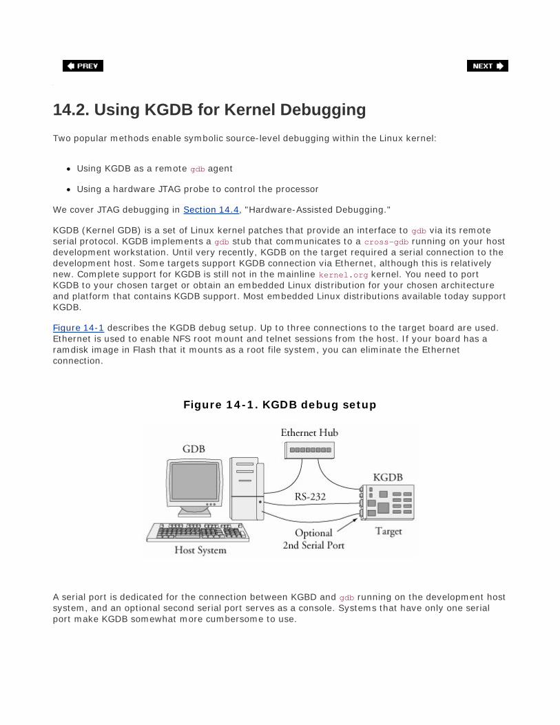
14.2. Using KGDB for Kernel Debugging
Two popular methods enable symbolic source-level debugging within the Linux kernel:
Using KGDB as a remote gdb agent
Using a hardware JTAG probe to control the processor
We cover JTAG debugging in Section 14.4, "Hardware-Assisted Debugging."
KGDB (Kernel GDB) is a set of Linux kernel patches that provide an interface to gdb via its remoteserial protocol. KGDB implements a gdb stub that communicates to a cross-gdb running on your hostdevelopment workstation. Until very recently, KGDB on the target required a serial connection to thedevelopment host. Some targets support KGDB connection via Ethernet, although this is relativelynew. Complete support for KGDB is still not in the mainline kernel.org kernel. You need to portKGDB to your chosen target or obtain an embedded Linux distribution for your chosen architectureand platform that contains KGDB support. Most embedded Linux distributions available today supportKGDB.
Figure 14-1 describes the KGDB debug setup. Up to three connections to the target board are used.Ethernet is used to enable NFS root mount and telnet sessions from the host. If your board has aramdisk image in Flash that it mounts as a root file system, you can eliminate the Ethernetconnection.
Figure 14-1. KGDB debug setup
A serial port is dedicated for the connection between KGBD and gdb running on the development hostsystem, and an optional second serial port serves as a console. Systems that have only one serialport make KGDB somewhat more cumbersome to use.

As you can see in Figure 14-1, the debugger (your cross-version of gdb) runs on your developmenthost system. KGDB is part of the kernel running on your target system. KGDB implements the hooksrequired to interface gdb with your target board to enable features such as setting breakpoints,examining memory, and enabling single-step program execution.
14.2.1. KGDB Kernel Configuration
KGDB is a kernel feature and must be enabled in your kernel. KGDB is selected from the KernelHacking menu, as shown in Figure 14-2. As part of the configuration, you must select the serial portfor KGDB to use. Notice also from Figure 14-2 that we enabled the option to compile the kernel withdebug information. This adds the -g compiler flag to the build process to enable symbolic debugging.
Figure 14-2. Kernel configuration for KGDB
[View full size image]

14.2.2. Target Boot with KGDB Support
After your kernel is built with KGDB support, it must be enabled. Unfortunately, the method to enableit is not yet uniform across all architectures and implementations. In general, KGDB is enabled bypassing a command line switch to the kernel via the kernel command line. If KGDB support iscompiled into the kernel but not enabled via a command line switch, it does nothing. When KGDB isenabled, the kernel stops at a KGDB-enabled breakpoint very early in the boot cycle to allow you toconnect to the target using gdb. Figure 14-3 shows the logic for generating an initial breakpoint whenKGDB is enabled.
Figure 14-3. KGDB logic
KGDB requires a serial port for connection to the host.[3] The first step in setting up KGDB is toenable a serial port very early in the boot process. In many architectures, the hardware UART mustbe mapped into kernel memory before access. After the address range is mapped, the serial port isinitialized. Debug trap handlers are installed to allow processor exceptions to trap into the debugger.
[3] Notwithstanding the comments made earlier about KGDB over Ethernet.
Listing 14-1 displays the terminal output when booting with KGDB enabled. This example is based onthe AMCC 440EP Evaluation Kit (Yosemite board), which ships with the U-Boot bootloader.

Listing 14-1. Booting with KGDB Enabled Using U-Boot
=> sete bootargs console=ttyS1,115200 root=/dev/nfs rw ip=dhcp gdb=> bootm 200000## Booting image at 00200000 ... Image Name: Linux-2.6.13 Image Type: PowerPC Linux Kernel Image (gzip compressed) Data Size: 1064790 Bytes = 1 MB Load Address: 00000000 Entry Point: 00000000 Verifying Checksum ... OK Uncompressing Kernel Image ... OK$T0440:c000ae5c;01:c0205fa0;#d9 <<< See text
Most of the boot sequence is familiar from our coverage of U-Boot in Chapter 7, "Bootloaders." Thiskernel boot sequence has two unique features: the command-line parameter to enable KGDB and theodd-looking text string after the kernel is uncompressed.
Recall from Chapter 7 that the kernel command line is defined by the U-Boot bootargs environmentvariable. Notice that we have added the gdb parameter, which instructs the kernel to force an earlybreakpoint and wait for the host debugger (your cross-gdb) to connect.
As diagrammed in Figure 14-3, the kernel detects the presence of the gdb parameter and attempts topass control to the remote (host-based) debugger. This is evidenced by the sequence of ASCIIcharacters dumped to the serial port in Listing 14-1. If you are curious about this gdb remote serialprotocol, it is documented in the gdb manual cited at the end of this chapter. In this example, KGDB issending a Stop Reply packet reporting the breakpoint trap to the remote gdb session on the host. Thetwo 32-bit parameters indicate the location of the program and the stack frame.
Now that the kernel is set up and waiting for the host debugger, we can begin our debugging session.We invoke cross-gdb from our host development workstation and connect to the target via gdb'sremote protocol. In this example, we are sharing the serial port, so we must disconnect the terminalemulator from the target before trying to connect with gdb. Listing 14-2 highlights the gdb connectionprocess. This assumes that we have already exited our terminal emulator and freed the serial port forgdb to use.
Listing 14-2. Connecting to KGDB

$ ppc_4xx-gdb --silent vmlinux(gdb) target remote /dev/ttyS0Remote debugging using /dev/ttyS0breakinst () at arch/ppc/kernel/ppc-stub.c:825825 }(gdb) l820 return;821 }822823 asm(" .globl breakinst \n\824 breakinst: .long 0x7d821008");825 }826827 #ifdef CONFIG_KGDB_CONSOLE828 /* Output string in GDB O-packet format if GDB has connected.If nothing829 output, returns 0 (caller must then handle output). */(gdb)
Here we have performed three actions:
Invoked gdb, passing it the kernel ELF file vmlinux
Connected to the target using the target remote command within gdb
Issued the list command, using its abbreviated form to display our location in the source code
At the risk of pointing out the obvious, the vmlinux image that we pass to gdb must be from the samekernel build that produced the target kernel binary. It also must have been compiled with the -gcompiler flag to contain debug information.
When we issued the target remote command, gdb responded by displaying the location of theprogram counter (PC). In this example, the kernel is stopped at the breakpoint defined by the inlineassembler statement at line 823 in file .../arch/ppc/kernel/ppc-stub.c. When we issue thecontinue (c) command, execution resumes starting at line 825, as indicated.
14.2.3. Useful Kernel Breakpoints
We have now established a debug connection with the kernel on our target board. When we issue thegdb continue (c) command, the kernel proceeds to boot, and if there are no problems, the bootprocess completes. There is one minor limitation of using KGDB on many architectures andprocessors. An engineering trade-off was made between the need to support very early kerneldebugging (for example, before a full-blown interrupt-driven serial port driver is installed) and thedesire to keep the complexity of the KGDB debug engine itself very simple and, therefore, robust andportable. KGDB uses a simple polled serial driver that has zero overhead when the kernel is running.As a drawback to this implementation, the traditional Ctl-C or Break sequence on the serial port willhave no effect. Therefore, it will be impossible to stop execution of the running kernel unless abreakpoint or other fault is encountered.

For this reason, it has become common practice to define some system-wide breakpoints, whichprovide the capability to halt the current thread of execution. Two of the most common arehighlighted in Listing 14-3.
Listing 14-3. Common Kernel Breakpoints
(gdb) b panicBreakpoint 1 at 0xc0016b18: file kernel/panic.c, line 74.(gdb) b sys_syncBreakpoint 2 at 0xc005a8c8: file fs/buffer.c, line 296.(gdb)
Using the gdb breakpoint command, again using its abbreviated version, we enter two breakpoints.One is at panic() and the other is at the sync system call entry sys_sync(). The former allows thedebugger to be invoked if a later event generates a panic. This enables examination of the systemstate at the time of the panic. The second is a useful way to halt the kernel and trap into thedebugger from user space by entering the sync command from a terminal running on your targethardware.
We are now ready to proceed with our debugging session. We have a KGDB-enabled kernel runningon our target, paused at a KGDB-defined early breakpoint. We established a connection to the targetwith our host-based cross debuggerin this case, invoked as ppc_4xx-gdband we have entered a pair ofuseful system breakpoints. Now we can direct our debugging activities to the task at hand.
One caveat: By definition, we cannot use KGDB for stepping through code before the breakpoint()function in .../arch/ppc/setup.c used to establish the connection between a KGDB-enabled kerneland cross-gdb on our host. Figure 14-3 is a rough guide to the code that executes before KGDB gainscontrol. Debugging this early code requires the use of a hardware-assisted debug probe. We coverthis topic shortly in Section 14.4, "Hardware-Assisted Debugging."

14.3. Debugging the Linux Kernel
One of the more common reasons you might find yourself stepping through kernel code is to modifyor customize the platform-specific code for your custom board. Let's see how this might be doneusing the AMCC Yosemite board. We place a breakpoint at the platform-specific architecture setupfunction and then continue until that breakpoint is encountered. Listing 14-4 shows the sequence.
Listing 14-4. Debugging Architecture-Setup Code
(gdb) b yosemite_setup_arch Breakpoint 3 at 0xc021a488: file arch/ppc/platforms/4xx/yosemite.c, line 308.(gdb) cContinuing.Can't send signals to this remote system. SIGILL not sent.
Breakpoint 3, yosemite_setup_arch () at arch/ppc/platforms/4xx/yosemite.c:308308 yosemite_set_emacdata();(gdb) l303 }304305 static void __init306 yosemite_setup_arch(void)307 {308 yosemite_set_emacdata();309310 ibm440gx_get_clocks(&clocks, YOSEMITE_SYSCLK, 6 * 1843200);311 ocp_sys_info.opb_bus_freq = clocks.opb;312 (gdb)
When the breakpoint at yosemite_setup_arch() is encountered, control passes to gdb at line 308 ofyosemite.c . The list (l ) command displays the source listing centered on the breakpoint at line308. The warning message displayed by gdb after the continue (c ) command can be safely ignored.It is part of gdb 's way of testing the capabilities of the remote system. It first sends a remotecontinue_with_signal command to the target. The KGDB implementation for this target board doesnot support this command; therefore, it is NAK 'd by the target. gdb responds by displaying thisinformational message and issuing the standard remote continue command instead.
14.3.1. gdb Remote Serial Protocol
gdb includes a debug switch that enables us to observe the remote protocol being used between gdb

on your development host and the target. This can be very useful for understanding the underlyingprotocol, as well as troubleshooting targets that exhibit unusual or errant behavior. To enable thisdebug mode, issue the following command:
(gdb) set debug remote 1
With remote debugging enabled, it is instructive to observe the continue command in action and thesteps taken by gdb . Listing 14-5 illustrates the use of the continue command with remote debuggingenabled.
Listing 14-5. continue Remote Protocol Example
(gdb) cContinuing.Sending packet: $mc0000000,4#80...AckPacket received: c022d200Sending packet: $Mc0000000,4:7d821008#68...AckPacket received: OKSending packet: $mc0016de8,4#f8...AckPacket received: 38600001Sending packet: $Mc0016de8,4:7d821008#e0...AckPacket received: OKSending packet: $mc005bd5c,4#23...AckPacket received: 38600001Sending packet: $Mc005bd5c,4:7d821008#0b...AckPacket received: OKSending packet: $mc021a488,4#c8...AckPacket received: 4bfffbadSending packet: $Mc021a488,4:7d821008#b0...AckPacket received: OKSending packet: $c#63...Ack <<< program running, gdb waiting for event
Although it might look daunting at first, what is happening here is easily understood. In summary,gdb is restoring all its breakpoints on the target. Recall from Listing 14-3 that we entered twobreakpoints, one at panic() and one at sys_sync() . Later in Listing 14-4 , we added a thirdbreakpoint at yosemite_setup_arch() . Thus, there are three active user-specified breakpoints. Thesecan be displayed by issuing the gdb info breakpoints command. As usual, we use the abbreviatedversion.
[View full width](gdb) i bNum Type Disp Enb Address What1 breakpoint keep y 0xc0016de8 in panic at kernel/panic.c:742 breakpoint keep y 0xc005bd5c in sys_sync at fs/buffer.c:2963 breakpoint keep y 0xc021a488 in yosemite_setup_arch at arch/ppc/platforms/4xx/yosemite.c:308 breakpoint already hit 1 time(gdb)

Now compare the previous breakpoint addresses with the addresses in the gdb remote $m packet inListing 14-5 . The $m packet is a "read target memory" command, and the $M packet is a "write targetmemory" command. Once for each breakpoint, the address of the breakpoint is read from targetmemory, stored away locally on the host by gdb (so it can be restored later), and replaced with thePowerPC TRap instruction twge r2, r2 (0x7d821008 ), which results in control passing back to thedebugger. Figure 14-4 illustrates this action.
Figure 14-4. gdb inserting target memory breakpoints
You might have noticed that gdb is updating four breakpoints, whereas we entered only three. Thefirst one at target memory location 0xc000_0000 is put there by gdb automatically upon startup. Thislocation is the base address of the linked kernel image from the ELF fileessentially, _start . It isequivalent to a breakpoint at main() for user space debugging and is done by gdb automatically. Theother three breakpoints are the ones we entered earlier.
The same thing happens in reverse when an event occurs that returns control to gdb . Listing 14-6details the action when our breakpoint at yosemite_setup_arch() is encountered.
Listing 14-6. Remote Protocol: Breakpoint Hit
Packet received: T0440:c021a488;01:c020ff90;Sending packet: $mc0000000,4#80...Ack <<< Read memory @c0000000Packet received: 7d821008Sending packet: $Mc0000000,4:c022d200#87...Ack <<< Write memoryPacket received: OKSending packet: $mc0016de8,4#f8...Ack

Packet received: 7d821008Sending packet: $Mc0016de8,4:38600001#a4...AckPacket received: OKSending packet: $mc005bd5c,4#23...AckPacket received: 7d821008Sending packet: $Mc005bd5c,4:38600001#cf...AckPacket received: OKSending packet: $mc021a488,4#c8...AckPacket received: 7d821008Sending packet: $Mc021a488,4:4bfffbad#d1...AckPacket received: OK
Sending packet: $mc021a484,c#f3...AckPacket received: 900100244bfffbad3fa0c022Breakpoint 3, yosemite_setup_arch () at arch/ppc/platforms/4xx/yosemite.c:308308 yosemite_set_emacdata();(gdb)
The $T packet is a gdb Stop Reply packet. It is sent by the target to gdb when a breakpoint isencountered. In our example, the $T packet returned the value of the program counter and registerr1 .[4] The rest of the activity is the reverse of that in Listing 14-5 . The PowerPC trap breakpointinstructions are removed, and gdb restores the original instructions to their respective memorylocations.
[4] As pointed out earlier, the gdb remote protocol is detailed in the gdb manual cited at the end of this chapter in Section 14.6.1 ,
"Suggestions for Additional Reading."
14.3.2. Debugging Optimized Kernel Code
At the start of this chapter, we said that one of the challenges identified in debugging kernel coderesults from compiler optimization. We noted that the Linux kernel is compiled by default withoptimization level -O2 . In the examples up to this point, we used -O1 optimization to simplify thedebugging task. Here we illustrate one of the many ways optimization can complicate debugging.
The related Internet mail lists are strewn with questions related to what appear to be broken tools.Sometimes the poster reports that his debugger is single-stepping backward or that his line numbersdo not line up with his source code. Here we present an example to illustrate the complexities thatoptimizing compilers bring to source-level debugging. In this example, the line numbers that gdbreports when a breakpoint is hit do not match up with the line numbers in our source file due tofunction inlining .
For this demonstration, we use the same debug code snippet as shown in Listing 14-4 . However, forthis example, we have compiled the kernel with the compiler optimization flag -O2 . This is the defaultfor the Linux kernel. Listing 14-7 shows the results of this debugging session.
Listing 14-7. Optimized Architecture-Setup Code
$ ppc_44x-gdb --silent vmlinux(gdb) target remote /dev/ttyS0Remote debugging using /dev/ttyS0
breakinst () at arch/ppc/kernel/ppc-stub.c:825825 }(gdb) b panicBreakpoint 1 at 0xc0016b18: file kernel/panic.c, line 74.(gdb) b sys_syncBreakpoint 2 at 0xc005a8c8: file fs/buffer.c, line 296.(gdb) b yosemite_setup_archBreakpoint 3 at 0xc020f438: file arch/ppc/platforms/4xx/yosemite.c, line 116.(gdb) cContinuing.
Breakpoint 3, yosemite_setup_arch () at arch/ppc/platforms/4xx/yosemite.c:116
116 def = ocp_get_one_device(OCP_VENDOR_IBM, OCP_FUNC_EMAC, 0);(gdb) l111 struct ocp_def *def;112 struct ocp_func_emac_data *emacdata;113114 /* Set mac_addr and phy mode for each EMAC */115116 def = ocp_get_one_device(OCP_VENDOR_IBM, OCP_FUNC_EMAC, 0);117 emacdata = def->additions;118 memcpy(emacdata->mac_addr, __res.bi_enetaddr, 6);119 emacdata->phy_mode = PHY_MODE_RMII;120(gdb) p yosemite_setup_arch$1 = {void (void)} 0xc020f41c <yosemite_setup_arch>
Referring back to Listing 14-4 , notice that the function yosemite_setup_arch() actually falls on line306 of the file yosemite.c . Compare that with Listing 14-7 . We hit the breakpoint, but gdb reportsthe breakpoint at file yosemite.c line 116. It appears at first glance to be a mismatch of line numbersbetween the debugger and the corresponding source code. Is this a gdb bug? First let's confirm whatthe compiler produced for debug information. Using the readelf [5] tool described in Chapter 13 ,"Development Tools," we can examine the debug information for this function produced by thecompiler.
[5] Remember to use your cross-version of readelffor example, ppc_44x-readelf for the PowerPC 44x architecture.
$ ppc_44x-readelf --debug-dump=info vmlinux | grep -u6 \ yosemite_setup_arch | tail -n 7 DW_AT_name : (indirect string, offset: 0x9c04): yosemite_setup_arch DW_AT_decl_file : 1 DW_AT_decl_line : 307 DW_AT_prototyped : 1 DW_AT_low_pc : 0xc020f41c DW_AT_high_pc : 0xc020f794 DW_AT_frame_base : 1 byte block: 51 (DW_OP_reg1)
We don't have to be experts at reading DWARF2 debug records[6] to recognize that the function in

question is reported at line 307 in our source file. We can confirm this using the addr2line utility, alsointroduced in Chapter 13 . Using the address derived from gdb in Listing 14-7 :
[6] A reference for the Dwarf debug specification appears at the end of this chapter in Section 14.6.1 , "Suggestions for Additional
Reading."
$ ppc_44x-addr2line -e vmlinux 0xc020f41c
arch/ppc/platforms/4xx/yosemite.c:307
At this point, gdb is reporting our breakpoint at line 116 of the yosemite.c file. To understand what ishappening, we need to look at the assembler output of the function as reported by gdb . Listing 14-8is the output from gdb after issuing the disassemble command on the yosemite_setup_arch()function.
Listing 14-8. Disassemble Function yosemite_setup_arch
(gdb) disassemble yosemite_setup_arch0xc020f41c <yosemite_setup_arch+0>: mflr r00xc020f420 <yosemite_setup_arch+4>: stwu r1,-48(r1)0xc020f424 <yosemite_setup_arch+8>: li r4,5120xc020f428 <yosemite_setup_arch+12>: li r5,00xc020f42c <yosemite_setup_arch+16>: li r3,41160xc020f430 <yosemite_setup_arch+20>: stmw r25,20(r1)0xc020f434 <yosemite_setup_arch+24>: stw r0,52(r1)0xc020f438 <yosemite_setup_arch+28>: bl 0xc000d344<ocp_get_one_device>0xc020f43c <yosemite_setup_arch+32>: lwz r31,32(r3)0xc020f440 <yosemite_setup_arch+36>: lis r4,-163500xc020f444 <yosemite_setup_arch+40>: li r28,20xc020f448 <yosemite_setup_arch+44>: addi r4,r4,214600xc020f44c <yosemite_setup_arch+48>: li r5,60xc020f450 <yosemite_setup_arch+52>: lis r29,-163500xc020f454 <yosemite_setup_arch+56>: addi r3,r31,480xc020f458 <yosemite_setup_arch+60>: lis r25,-163500xc020f45c <yosemite_setup_arch+64>: bl 0xc000c708<memcpy>0xc020f460 <yosemite_setup_arch+68>: stw r28,44(r31)0xc020f464 <yosemite_setup_arch+72>: li r4,5120xc020f468 <yosemite_setup_arch+76>: li r5,10xc020f46c <yosemite_setup_arch+80>: li r3,41160xc020f470 <yosemite_setup_arch+84>: addi r26,r25,151040xc020f474 <yosemite_setup_arch+88>: bl 0xc000d344<ocp_get_one_device>0xc020f478 <yosemite_setup_arch+92>: lis r4,-163500xc020f47c <yosemite_setup_arch+96>: lwz r31,32(r3)0xc020f480 <yosemite_setup_arch+100>: addi r4,r4,215340xc020f484 <yosemite_setup_arch+104>: li r5,60xc020f488 <yosemite_setup_arch+108>: addi r3,r31,480xc020f48c <yosemite_setup_arch+112>: bl 0xc000c708<memcpy>

0xc020f490 <yosemite_setup_arch+116>: lis r4,10170xc020f494 <yosemite_setup_arch+120>: lis r5,1680xc020f498 <yosemite_setup_arch+124>: stw r28,44(r31)0xc020f49c <yosemite_setup_arch+128>: ori r4,r4,165540xc020f4a0 <yosemite_setup_arch+132>: ori r5,r5,491520xc020f4a4 <yosemite_setup_arch+136>: addi r3,r29,-153800xc020f4a8 <yosemite_setup_arch+140>: addi r29,r29,-153800xc020f4ac <yosemite_setup_arch+144>: bl 0xc020e338<ibm440gx_get_clocks>0xc020f4b0 <yosemite_setup_arch+148>: li r0,00xc020f4b4 <yosemite_setup_arch+152>: lis r11,-163520xc020f4b8 <yosemite_setup_arch+156>: ori r0,r0,500000xc020f4bc <yosemite_setup_arch+160>: lwz r10,12(r29)0xc020f4c0 <yosemite_setup_arch+164>: lis r9,-163520xc020f4c4 <yosemite_setup_arch+168>: stw r0,8068(r11)0xc020f4c8 <yosemite_setup_arch+172>: lwz r0,84(r26)0xc020f4cc <yosemite_setup_arch+176>: stw r10,8136(r9)0xc020f4d0 <yosemite_setup_arch+180>: mtctr r00xc020f4d4 <yosemite_setup_arch+184>: bctrl0xc020f4d8 <yosemite_setup_arch+188>: li r5,640xc020f4dc <yosemite_setup_arch+192>: mr r31,r30xc020f4e0 <yosemite_setup_arch+196>: lis r4,-42880xc020f4e4 <yosemite_setup_arch+200>: li r3,00xc020f4e8 <yosemite_setup_arch+204>: bl 0xc000c0f8<ioremap64>End of assembler dump.(gdb)
Once again, we need not be PowerPC assembly language experts to understand what is happeninghere. Notice the labels associated with the PowerPC bl instruction. This is a function call in PowerPCmnemonics. The symbolic function labels are the important data points. After a cursory analysis, wesee several function calls near the start of this assembler listing:
Address
Function
0xc020f438
ocp_get_one_device()
0xc020f45c
memcpy()
0xc020f474
ocp_get_one_device()
0xc020f48c

memcpy()
0xc020f4ac
ibm440gx_get_clocks()
Listing 14-9 reproduces portions of the source file yosemite.c . Correlating the functions we found inthe gdb disassemble output, we see those labels occurring in the function yosemite_set_emacdata() ,around the line numbers reported by gdb when the breakpoint at yosemite_setup_arch() wasencountered. The key to understanding the anomaly is to notice the subroutine call at the very startof yosemite_setup_arch() . The compiler has inlined the call to yosemite_set_emacdata() instead ofgenerating a function call, as would be expected by simple inspection of the source code. This inliningproduced the mismatch in the line numbers when gdb hit the breakpoint. Even though theyosemite_set_emacdata() function was not declared using the inline keyword, GCC inlined thefunction as a performance optimization.
Listing 14-9. Portions of Source File yosemite.c
109 static void __init yosemite_set_emacdata(void)110 {111 struct ocp_def *def;112 struct ocp_func_emac_data *emacdata;113114 /* Set mac_addr and phy mode for each EMAC */115116 def = ocp_get_one_device(OCP_VENDOR_IBM, OCP_FUNC_EMAC, 0);117 emacdata = def->additions;118 memcpy(emacdata->mac_addr, __res.bi_enetaddr, 6);119 emacdata->phy_mode = PHY_MODE_RMII;120121 def = ocp_get_one_device(OCP_VENDOR_IBM, OCP_FUNC_EMAC, 1);122 emacdata = def->additions;123 memcpy(emacdata->mac_addr, __res.bi_enet1addr, 6);124 emacdata->phy_mode = PHY_MODE_RMII;125 }126...304305 static void __init306 yosemite_setup_arch(void)307 {308 yosemite_set_emacdata();309310 ibm440gx_get_clocks(&clocks, YOSEMITE_SYSCLK, 6 * 1843200);311 ocp_sys_info.opb_bus_freq = clocks.opb;312313 /* init to some ~sane value until calibrate_delay() runs */314 loops_per_jiffy = 50000000/HZ;315316 /* Setup PCI host bridge */
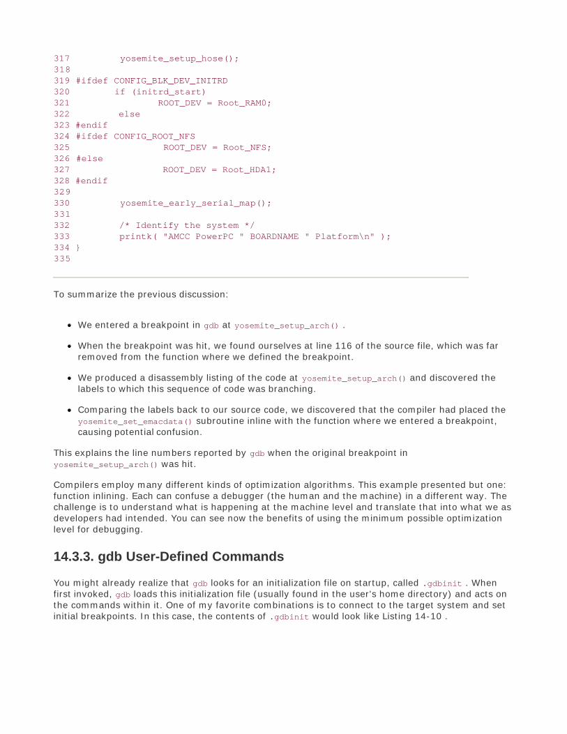
317 yosemite_setup_hose();318319 #ifdef CONFIG_BLK_DEV_INITRD320 if (initrd_start)321 ROOT_DEV = Root_RAM0;322 else323 #endif324 #ifdef CONFIG_ROOT_NFS325 ROOT_DEV = Root_NFS;326 #else327 ROOT_DEV = Root_HDA1;328 #endif329330 yosemite_early_serial_map();331332 /* Identify the system */333 printk( "AMCC PowerPC " BOARDNAME " Platform\n" );334 }335
To summarize the previous discussion:
We entered a breakpoint in gdb at yosemite_setup_arch() .
When the breakpoint was hit, we found ourselves at line 116 of the source file, which was farremoved from the function where we defined the breakpoint.
We produced a disassembly listing of the code at yosemite_setup_arch() and discovered thelabels to which this sequence of code was branching.
Comparing the labels back to our source code, we discovered that the compiler had placed theyosemite_set_emacdata() subroutine inline with the function where we entered a breakpoint,causing potential confusion.
This explains the line numbers reported by gdb when the original breakpoint inyosemite_setup_arch() was hit.
Compilers employ many different kinds of optimization algorithms. This example presented but one:function inlining. Each can confuse a debugger (the human and the machine) in a different way. Thechallenge is to understand what is happening at the machine level and translate that into what we asdevelopers had intended. You can see now the benefits of using the minimum possible optimizationlevel for debugging.
14.3.3. gdb User-Defined Commands
You might already realize that gdb looks for an initialization file on startup, called .gdbinit . Whenfirst invoked, gdb loads this initialization file (usually found in the user's home directory) and acts onthe commands within it. One of my favorite combinations is to connect to the target system and setinitial breakpoints. In this case, the contents of .gdbinit would look like Listing 14-10 .

Listing 14-10. Simple gdb Initialization File
$ cat ~/.gdbinitset history save onset history filename ~/.gdb_historyset output-radix 16
define connect# target remote bdi:2001 target remote /dev/ttyS0 b panic b sys_syncend
This simple .gdbinit file enables the storing of command history in a user-specified file and sets thedefault output radix for printing of values. Then it defines a gdb user-defined command called connect. (User-defined commands are also often called macros.) When issued at the gdb command prompt,gdb connects to the target system via the desired method and sets the system breakpoints atpanic() and sys_sync() . One method is commented out; we discuss this method shortly in Section14.4 .
There is no end to the creative use of gdb user-defined commands. When debugging in the kernel, itis often useful to examine global data structures such as task lists and memory maps. Here wepresent several useful gdb user-defined commands capable of displaying specific kernel data that youmight need to access during your kernel debugging.
14.3.4. Useful Kernel gdb Macros
During kernel debugging, it is often useful to view the processes that are running on the system, aswell as some common attributes of those processes. The kernel maintains a linked list of tasksdescribed by struct task_struct . The address of the first task in the list is contained in the kernelglobal variable init_task , which represents the initial task spawned by the kernel during startup.Each task contains a struct list_head , which links the tasks in a circular linked list. These twoubiquitous kernel structures are described in the following header files:
struct task_struct .../include/linux/sched.hstruct list_head .../include/linux/list.h
Using gdb macros, we can traverse the task list and display useful information about the tasks. It iseasy to modify the macros to extract the data you might be interested in. It is also a very useful toolfor learning the details of kernel internals.
The first macro we examine (in Listing 14-11 ) is a simple one that searches the kernel's linked list oftask_struct structures until it finds the given task. If it is found, it displays the name of the task.
Listing 14-11. gdb find_task Macro

1 # Helper function to find a task given a PID or the 2 # address of a task_struct. 3 # The result is set into $t 4 define find_task 5 # Addresses greater than _end: kernel data... 6 # ...user passed in an address 7 if ((unsigned)$arg0 > (unsigned)&_end) 8 set $t=(struct task_struct *)$arg0 9 else10 # User entered a numeric PID11 # Walk the task list to find it12 set $t=&init_task13 if (init_task.pid != (unsigned)$arg0)14 find_next_task $t15 while (&init_task!=$t && $t->pid != (unsigned)$arg0)16 find_next_task $t17 end18 if ($t == &init_task)19 printf "Couldn't find task; using init_task\n"20 end21 end22 end23 printf "Task \"%s\":\n", $t->comm24 end
Place this text into your .gdbinit file and restart gdb , or source[7] it using gdb's source command.(We explain the find_next_task macro later in Listing 14-15 .) Invoke it as follows:
[7] A helpful shortcut for macro development is the gdb source command. This command opens and reads a source file
containing macro definitions.
(gdb) find_task 910 Task "syslogd":
or
(gdb) find_task 0xCFFDE470 Task "bash":
Line 4 defines the macro name. Line 7 decides whether the input argument is a PID (numeric entrystarting at zero and limited to a few million) or a task_struct address that must be greater than theend of the Linux kernel image itself, defined by the symbol _end .[8] If it's an address, the only actionrequired is to cast it to the proper type to enable dereferencing the associated task_struct . This isdone at line 8. As the comment in line 3 states, this macro returns a gdb convenience variabletypecasted to a pointer to a struct task_struct .
[8] The symbol _end is defined in the linker script file during the final link.
If the input argument is a numeric PID, the list is traversed to find the matching task_struct . Lines12 and 13 initialize the loop variables (gdb does not have a for statement in its macro command

language), and lines 15 through 17 define the search loop. The find_next_task macro is used toextract the pointer to the next task_struct in the linked list. Finally, if the search fails, a sane returnvalue is set (the address of init_task ) so that it can be safely used in other macros.
Building on the find_task macro in Listing 14-11 , we can easily create a simple ps command thatdisplays useful information about each process running on the system.
Listing 14-12 defines a gdb macro that displays interesting information from a running process,extracted from the struct task_struct for the given process. It is invoked like any other gdbcommand, by typing its name followed by any required input parameters. Notice that this user-defined command requires a single argument, either a PID or the address of a task_struct .
Listing 14-12. gdb Macro: Print Process Information
1 define ps 2 # Print column headers 3 task_struct_header 4 set $t=&init_task 5 task_struct_show $t 6 find_next_task $t 7 # Walk the list 8 while &init_task!=$t 9 # Display useful info about each task10 task_struct_show $t11 find_next_task $t12 end13 end1415 document ps16 Print points of interest for all tasks17 end
This ps macro is similar to the find_task macro, except that it requires no input arguments and itadds a macro (task_struct_show ) to display the useful information from each task_struct . Line 3prints a banner line with column headings. Lines 4 through 6 set up the loop and display the firsttask. Lines 8 through 11 loop through each task, calling the task_struct_show macro for each.
Notice also the inclusion of the gdb document command. This allows the gdb user to get help byissuing the help ps command from the gdb command prompt as follows:
(gdb) help ps Print points of interest for all tasks
Listing 14-13 displays the output of this macro on a target board running only minimal services.
Listing 14-13. gdb ps Macro Output
(gdb) psAddress PID State User_NIP Kernel-SP device comm

0xC01D3750 0 Running 0xC0205E90 (none) swapper0xC04ACB10 1 Sleeping 0x0FF6E85C 0xC04FFCE0 (none) init0xC04AC770 2 Sleeping 0xC0501E90 (none) ksoftirqd/00xC04AC3D0 3 Sleeping 0xC0531E30 (none) events/00xC04AC030 4 Sleeping 0xC0533E30 (none) khelper0xC04CDB30 5 Sleeping 0xC0535E30 (none) kthread0xC04CD790 23 Sleeping 0xC06FBE30 (none) kblockd/00xC04CD3F0 45 Sleeping 0xC06FDE50 (none) pdflush0xC04CD050 46 Sleeping 0xC06FFE50 (none) pdflush0xC054B7B0 48 Sleeping 0xC0703E30 (none) aio/00xC054BB50 47 Sleeping 0xC0701E20 (none) kswapd00xC054B410 629 Sleeping 0xC0781E60 (none) kseriod0xC054B070 663 Sleeping 0xCFC59E30 (none) rpciod/00xCFFDE0D0 675 Sleeping 0x0FF6E85C 0xCF86DCE0 (none) udevd0xCF95B110 879 Sleeping 0x0FF0BE58 0xCF517D80 (none) portmap0xCFC24090 910 Sleeping 0x0FF6E85C 0xCF61BCE0 (none) syslogd0xCF804490 918 Sleeping 0x0FF66C7C 0xCF65DD70 (none) klogd0xCFE350B0 948 Sleeping 0x0FF0E85C 0xCF67DCE0 (none) rpc.statd0xCFFDE810 960 Sleeping 0x0FF6E85C 0xCF5C7CE0 (none) inetd
0xCFC24B70 964 Sleeping 0x0FEEBEAC 0xCF64FD80 (none) mvltd0xCFE35B90 973 Sleeping 0x0FF66C7C 0xCFEF7CE0 ttyS1 getty0xCFE357F0 974 Sleeping 0x0FF4B85C 0xCF6EBCE0 (none) in.telnetd0xCFFDE470 979 Sleeping 0x0FEB6950 0xCF675DB0 ttyp0 bash0xCFFDEBB0 982<Running 0x0FF6EB6C 0xCF7C3870 ttyp0 sync(gdb)
The bulk of the work done by this ps macro is performed by the task_struct_show macro. As shownin Listing 14-13 , the task_struct_show macro displays the following fields from each task_struct :
Address Address of the task_struct for the process
PID Process ID
State Current state of the process
User_NIP Userspace Next Instruction Pointer
Kernel_SP Kernel Stack Pointer
device Device associated with this process
comm Name of the process (or command)
It is relatively easy to modify the macro to show the items of interest for your particular kerneldebugging task. The only complexity is in the simplicity of the macro language. Because functionequivalents such as strlen do not exist in gdb 's user-defined command language, screen formattingmust be done by hand.
Listing 14-14 reproduces the task_struct_show macro that produced the previous listing.

Listing 14-14. gdb task_struct_show Macro
1 define task_struct_show 2 # task_struct addr and PID 3 printf "0x%08X %5d", $arg0, $arg0->pid 4 5 # Place a '<' marker on the current task 6 # if ($arg0 == current) 7 # For PowerPC, register r2 points to the "current" task 8 if ($arg0 == $r2) 9 printf "<"10 else11 printf " "12 end1314 # State15 if ($arg0->state == 0)16 printf "Running "17 else18 if ($arg0->state == 1)19 printf "Sleeping "20 else21 if ($arg0->state == 2)22 printf "Disksleep "23 else24 if ($arg0->state == 4)25 printf "Zombie "26 else27 if ($arg0->state == 8)28 printf "sTopped "29 else30 if ($arg0->state == 16)31 printf "Wpaging "32 else33 printf "%2d ", $arg0->state34 end35 end36 end37 end38 end39 end4041 # User NIP42 if ($arg0->thread.regs)43 printf "0x%08X ", $arg0->thread.regs->nip44 else45 printf " "46 end4748 # Display the kernel stack pointer49 printf "0x%08X ", $arg0->thread.ksp50

51 # device52 if ($arg0->signal->tty)53 printf "%s ", $arg0->signal->tty->name54 else55 printf "(none) "56 end5758 # comm59 printf "%s\n", $arg0->comm60 end
Line 3 displays the address of the task_struct . Lines 8 through 12 display the process ID. If this isthe current process (the process that was currently running on this CPU at the time the breakpointwas hit), it is marked with a < character.
Lines 14 through 39 decode and display the state of the process. This is followed by displaying theuser process next instruction pointer (NIP) and the kernel stack pointer (SP). Finally, the deviceassociated with the process is displayed, followed by the name of the process (stored in the ->commelement of the task_struct .)
It is important to note that this macro is architecture dependent, as shown in lines 7 and 8. Ingeneral, macros such as these are highly architecture- and version-dependent. Any time a change inthe underlying structure is made, macros such as these must be updated. However, if you spend alot of time debugging the kernel using gdb , the payback is often worth the effort.
For completeness, we present the find_next_task macro. Its implementation is less than obvious anddeserves explanation. (It is assumed that you can easily deduce the task_struct_header thatcompletes the series necessary for the ps macro presented in this section. It is nothing more than asingle line arranging the column headers with the correct amount of whitespace.) Listing 14-15presents the find_next_task macro used in our ps and find_task macros.
Listing 14-15. gdb find_next_task Macro
define find_next_task # Given a task address, find the next task in the linked list set $t = (struct task_struct *)$arg0 set $offset=( (char *)&$t->tasks - (char *)$t) set $t=(struct task_struct *)( (char *)$t->tasks.next- (char *)$offset)end
The function performed by this macro is simple. The implementation is slightly less thanstraightforward. The goal is to return the ->next pointer, which points to the next task_struct on thelinked list. However, the task_struct structures are linked by the address of the struct list_headmember called tasks , as opposed to the common practice of being linked by the starting address ofthe task_struct itself. Because the ->next pointer points to the address of the task structure elementin the next task_struct on the list, we must subtract to get the address of the top of the task_structitself. The value we subtract from the ->next pointer is the offset from that pointer's address to thetop of task_struct . First we calculate the offset and then we use that offset to adjust the ->nextpointer to point to the top of task_struct . Figure 14-5 should make this clear.

Figure 14-5. Task structure list linking
Now we present one final macro that will be useful in the next section when we discuss debuggingloadable modules. Listing 14-16 is a simple macro that displays the kernel's list of currently installedloadable modules.
Listing 14-16. gdb List Modules Macro
1 define lsmod2 printf "Address\t\tModule\n"3 set $m=(struct list_head *)&modules4 set $done=05 while ( !$done )6 # list_head is 4-bytes into struct module7 set $mp=(struct module *)((char *)$m->next - (char *)4)8 printf "0x%08X\t%s\n", $mp, $mp->name9 if ( $mp->list->next == &modules)10 set $done=111 end12 set $m=$m->next13 end14 end1516 document lsmod17 List the loaded kernel modules and their start addresses18 end

This simple loop starts with the kernel's global variable module . This variable is a struct list_headthat marks the start of the linked list of loadable modules. The only complexity is the same as thatdescribed in Listing 14-15 . We must subtract an offset from the struct list_head pointer to point tothe top of the struct module . This is performed in line 7. This macro produces a simple listing ofmodules containing the address of the struct module and the module's name. Here is an example ofits use:
(gdb) lsmodAddress Module0xD1012A80 ip_conntrack_tftp0xD10105A0 ip_conntrack0xD102F9A0 loop(gdb) help lsmodList the loaded kernel modules and their start addresses(gdb)
Macros such as the ones presented here are very powerful debugging aids. You can create macros ina similar fashion to display anything in the kernel that lends itself to easy access, especially the majordata structures maintained as linked lists. Examples include process memory map information,module information, file system information, and timer lists and so on. The information presentedhere should get you started.
14.3.5. Debugging Loadable Modules
The most common reason for using KGDB is to debug loadable kernel modules, that is, devicedrivers. One of the more convenient features of loadable modules is that, under most circumstances,it is not necessary to reboot the kernel for each new debugging session. You can start a debuggingsession, make some changes, recompile, and reload the module without the hassle and delay of acomplete kernel reboot.
The complication associated with debugging loadable modules is in gaining access to the symbolicdebug information contained in the module's object file. Because loadable modules are dynamicallylinked when they are loaded into the kernel, the symbolic information contained in the object file isuseless until the symbol table is adjusted.
Recall from our earlier examples how we invoke gdb for a kernel debugging session:
$ ppc_4xx-gdb vmlinux
This launches a gdb debugging session on your host, and reads the symbol information from theLinux kernel ELF file vmlinux . Of course, you will not find symbols for any loadable modules in thisfile. Loadable modules are separate compilation units and are linked as individual standalone ELFobjects. Therefore, if we intend to perform any source-level debugging on a loadable module, weneed to load its debug symbols from the ELF file. gdb provides this capability in its add-symbol-filecommand.
The add-symbol-file command loads symbols from the specified object file, assuming that the

module itself has already been loaded. However, we are faced with the chicken-and-egg syndrome.We don't have any symbol information until the loadable module has been loaded into the kernel andthe add-symbol-file command is issued to read in the module's symbol information. However, afterthe module has been loaded, it is too late to set breakpoints and debug the module's *_init andrelated functions because they have already executed.
The solution to this dilemma is to place a breakpoint in the kernel code that is responsible for loadingthe module, after it has been linked but before its initialization function has been called. This work isdone by .../kernel/module.c . Listing 14-17 reproduces the relevant portions of module.c .
Listing 14-17. module.c : Module Initialization
...1901 down(¬ify_mutex);1902 notifier_call_chain(&module_notify_list, MODULE_STATE_COMING, mod);1903 up(¬ify_mutex);19041905 /* Start the module */1906 if (mod->init != NULL)1907 ret = mod->init();1908 if (ret < 0) {1909 /* Init routine failed: abort. Try to protect us from1910 buggy refcounters. */1911 mod->state = MODULE_STATE_GOING;...
We load the module using the modprobe utility, which was demonstrated in Listing 8-5 in Chapter 8 ,"Device Driver Basics," and looks like this:
$ modprobe loop
This command issues a special system call that directs the kernel to load the module. The moduleloading begins at sys_init_module() in module.c . After the module has been loaded into kernelmemory and dynamically linked, control is passed to the module's _init function. This is shown inlines 1906 and 1907 of Listing 14-17 . We place our breakpoint here. This enables us to add thesymbol file to gdb and subsequently set breakpoints in the module. We demonstrate this processusing the Linux kernel's loopback driver called loop.ko . This module has no dependencies on othermodules and is reasonably easy to demonstrate.
Listing 14-18 shows the gdb commands to initiate this debugging session on loop.ko .
Listing 14-18. Initiate Module Debug Session: loop.ko
1 $ ppc-linux-gdb --silent vmlinux2 (gdb) connect3 breakinst () at arch/ppc/kernel/ppc-stub.c:8254 825 }5 Breakpoint 1 at 0xc0016b18: file kernel/panic.c, line 74.6 Breakpoint 2 at 0xc005a8c8: file fs/buffer.c, line 296.

7 (gdb) b module.c:19078 Breakpoint 3 at 0xc003430c: file kernel/module.c, line 1907.9 (gdb) c10 Continuing.11 >>>> Here we let the kernel finish booting12 and then load the loop.ko module on the target1314 Breakpoint 3, sys_init_module (umod=0x30029000, len=0x2473e,15 uargs=0x10016338 "") at kernel/module.c:190716 1907 ret = mod->init();17 (gdb) lsmod18 Address Module19 0xD102F9A0 loop20 (gdb) set $m=(struct module *)0xD102F9A0.21 (gdb) p $m->module_core22 $1 = (void *) 0xd102c00023 (gdb) add-symbol-file ./drivers/block/loop.ko 0xd102c00024 add symbol table from file "./drivers/block/loop.ko" at25 .text_addr = 0xd102c00026 (y or n) y27 Reading symbols from /home/chris/sandbox/linux-2.6.13-amcc/drivers/block /loop.ko...done.
Starting with line 2, we use the gdb user-defined macro connect created earlier in Listing 14-10 toconnect to the target board and set our initial breakpoints. We then add the breakpoint in module.c ,as shown in line 7, and we issue the continue command (c) . Now the kernel completes the bootprocess and we establish a telnet session into the target and load the loop.ko module (not shown).When the loopback module is loaded, we immediately hit breakpoint #3. gdb then displays theinformation shown in lines 14 through 16.
At this point, we need to discover the address where the Linux kernel linked our module's .textsection. Linux stores this address in the module information structure struct module in themodule_core element. Using the lsmod macro we defined in Listing 14-16 , we obtain the address ofthe struct module associated with our loop.ko module. This is shown in lines 17 through 19. Now weuse this structure address to obtain the module's .text address from the module_core structuremember. We pass this address to the gdb add-symbol-file command, and gdb uses this address toadjust its internal symbol table to match the actual addresses where the module was linked into thekernel. From there, we can proceed in the usual manner to set breakpoints in the module, stepthrough code, examine data, and so on.
We conclude this section with a demonstration of placing a breakpoint in the loopback module'sinitialization function so that we can step through the module's initialization code. The complicationhere is that the kernel loads the module's initialization code into a separately allocated portion ofmemory so that it can be freed after use. Recall from Chapter 5 , "Kernel Initialization," ourdiscussion of the __init macro. This macro expands into a compiler attribute that directs the linker toplace the marked portion of code into a specially named ELF section. In essence, any function definedwith this attribute is placed in a separate ELF section named .init.text . Its use is similar to thefollowing:
static int __init loop_init(void){...}

This invocation would place the compiled loop_init() function into the .init.text section of theloop.ko object module. When the module is loaded, the kernel allocates a chunk of memory for themain body of the module, which is pointed to by the struct module member named module_core . Itthen allocates a separate chunk of memory to hold the .init.text section. After the initializationfunction is called, the kernel frees the memory that contained the initialization function. Because theobject module is split like this, we need to inform gdb of this addressing scheme to be able to usesymbolic data for debugging the initialization function.[9] Listing 14-19 demonstrates these steps.
[9] As of this writing, there is a bug in gdb that prevents this technique from working properly. Hopefully, by the time you read this,
it will be fixed.
Listing 14-19. Debugging Module init Code
$ ppc_4xx-gdb -slient vmlinux(gdb) target remote /dev/ttyS0Remote debugging using /dev/ttyS0breakinst () at arch/ppc/kernel/ppc-stub.c:825825 }<< Place a breakpoint before calling module init >>(gdb) b module.c:1907Breakpoint 1 at 0xc0036418: file kernel/module.c, line 1907.(gdb) cContinuing.
Breakpoint 1, sys_init_module (umod=0xd102ef40, len=0x23cb3, uargs=0x10016338 "")at kernel/module.c:19071907 ret = mod->init();
<< Discover init addressing from struct module >>(gdb) lsmodAddress Module0xD102EF40 loop(gdb) set $m=(struct module *)0xD102EF40(gdb) p $m->module_core$1 = (void *) 0xd102b000(gdb) p $m->module_init$2 = (void *) 0xd1031000<< Now load a symbol file using the core and init addrs >>(gdb) add-symbol-file ./drivers/block/loop.ko 0xd102b000 -s .init.text 0xd1031000add symbol table from file "./drivers/block/loop.ko" at .text_addr = 0xd102b000 .init.text_addr = 0xd1031000(y or n) yReading symbols from /home/chris/sandbox/linux-2.6.13-amcc/drivers/block/loop.ko...done.(gdb) b loop_initBreakpoint 3 at 0xd1031000: file drivers/block/loop.c, line 1244.(gdb) cContinuing.<< Breakpoint hit, proceed to debug module init function >>Breakpoint 3, 0xd1031000 in loop_init () file drivers/block/loop.c, line 12441244 if (max_loop < 1 || max_loop > 256) {

(gdb)
14.3.6. printk Debugging
Debugging kernel and device driver code using printk is a popular technique, mostly because printkhas evolved into a very robust method. You can call printk from almost any context, including frominterrupt handlers. printk is the kernel's version of the familiar printf() C library function. printk isdefined in .../kernel/printk.c .
It is important to understand the limitations of using printk for debugging. First, printk requires aconsole device. Moreover, although the console device is configured as early as possible during kernelinitialization, there are many calls to printk before the console device has been initialized. Wepresent a method to cope with this limitation later, in Section 14.5 , "When It Doesn't Boot."
The printk function allows the addition of a string marker that identifies the level of severity of agiven message. The header file .../include/linux/kernel.h defines eight levels:
#define KERN_EMERG "<0>" /* system is unusable */#define KERN_ALERT "<1>" /* action must be taken immediately */#define KERN_CRIT "<2>" /* critical conditions */#define KERN_ERR "<3>" /* error conditions */#define KERN_WARNING "<4>" /* warning conditions */#define KERN_NOTICE "<5>" /* normal but significant condition */#define KERN_INFO "<6>" /* informational */#define KERN_DEBUG "<7>" /* debug-level messages */
A simple printk message might look like this:
printk("foo() entered w/ %s\n", arg);
If the severity string is omitted, the kernel assigns a default severity level, which is defined inprintk.c . In recent kernels, this is set at severity level 4, KERN_WARNING . Specifying printk with aseverity level might look something like this:
printk(KERN_CRIT "vmalloc failed in foo()\n");
By default, all printk messages below a predefined loglevel are displayed on the system consoledevice. The default loglevel is defined in printk.c . In recent Linux kernels, it has the value 7 . Thismeans that any printk message that is greater in importance than KERN_DEBUG will be displayed onthe console.
You can set the default kernel loglevel in a variety of ways. At boot time, you can specify the defaultloglevel on your target board by passing the appropriate kernel command line parameters to thekernel at boot time. Three kernel command line options defined in main.c affect the default loglevel:
debug Sets the console loglevel to 10

quiet Sets the console loglevel to 4
loglevel= Sets the console loglevel to your choice of value
Using debug effectively displays every printk message. Using quiet displays all printk messages ofseverity KERN_ERR or higher.
printk messages can be logged to files on your target or via the network. Use klogd (kernel logdaemon) and syslogd (system log daemon) to control the logging behavior of printk messages.These popular utilities are described in man pages and many Linux references, and are not describedhere.
14.3.7. Magic SysReq Key
This useful debugging aid is invoked through a series of special predefined key sequences that sendmessages directly to the kernel. For many target architectures and boards, you use a simple terminalemulator on a serial port as a system console. For these architectures, the Magic SysReq key isdefined as a break character followed by a command character. Consult the documentation on theterminal emulator you use for how to send a break character. Many Linux developers use the minicomterminal emulator. For minicom , the break character is sent by typing Ctl-A F . After sending thebreak in this manner, you have 5 seconds to enter the command character before the commandtimes out.
This useful kernel tool can be very helpful for development and debugging, but it can also cause dataloss and system corruption. Indeed, the b command immediately reboots your system without anynotification or preparation. Open files are not closed, disks are not synced, and file systems are notunmounted. When the reboot (b ) command is issued, control is immediately passed to the resetvector of your architecture in a most abrupt and stunning manner. Use this powerful tool at your ownperil!
This feature is well documented in the Linux kernel documentation subdirectory in a file calledsysrq.txt . There you find the details for many architectures and the description of availablecommands.
For example, another way to set the kernel loglevel just discussed is to use the Magic SysReq key.The command is a number from 0 through 9, which results in the default loglevel being set to thenumber of the command. From minicom, press Ctl-A F followed by a number, such as 9. Here is howit looks on the terminal:
$ SysRq : Changing Loglevel Loglevel set to 9
Commands can be used to dump registers, shut down your system, reboot your system, dump a listof processes, dump current memory information to your console, and more. See the documentationfile in any recent Linux kernel for the details.
This feature is most commonly used when something causes your system to lock up. Often the MagicSysReq key provides a way to learn something from an otherwise dead system.


14.4. Hardware-Assisted Debugging
By now you've probably realized that you cannot debug very early kernel-startup code with KGDB.This is because KGDB is not initialized until after most of the low-level hardware-initialization codehas executed. Furthermore, if you are assigned the task of bringing up a brand-new board designand porting a bootloader and the Linux kernel, having a hardware-debug probe is without a doubt themost efficient means of debugging problems in these early stages of board porting.
You can choose from a wide variety of hardware-debug probes. For the examples in this section, weuse a unit manufactured by Abatron called the BDI-2000 (see www.abatron.ch). These units areoften called JTAG probes because they use a low-level communications method that was firstemployed for boundary scan testing of integrated circuits defined by the Joint Test Action Group(JTAG).
A JTAG probe contains a small connector designed for connection to your target board. It is often asimple square-pin header and ribbon cable arrangement. Most modern high-performance CPUscontain a JTAG interface that is designed to provide this software debugging capability. The JTAGprobe connects to this CPU JTAG interface. The other side of the JTAG probe connects to your hostdevelopment system usually via Ethernet, USB, or a parallel port. Figure 14-6 details the setup forthe Abatron unit.
Figure 14-6. Hardware JTAG probe debugging
JTAG probes can be complicated to set up. This is a direct result of the complexity of the CPU towhich it is connected. When power is applied to a target board and its CPU comes out of reset, almostnothing is initialized. In fact, many processors need at least a small amount of initialization beforethey can do anything. Many methods are available for getting this initial configuration into the CPU.Some CPUs read a hardware-configuration word or initial values of specific pins to learn their power-

on configuration. Others rely on reading a default location in a simple nonvolatile storage device suchas Flash. When using a JTAG probe, especially for bringing up a new board design, a minimum levelof CPU and board initialization must be performed before anything else can be done. Many JTAGprobes rely on a configuration file for this initialization.
The Abatron unit uses a configuration file to initialize the target hardware it is connected to, as wellas to define other operational parameters of the debugger. This configuration file contains directivesthat initialize the CPU, memory system, and other necessary board-level hardware. It is thedeveloper's responsibility to customize this configuration file with the proper directives for his ownboard. The details on the configuration command syntax can be found in the JTAG probe'sdocumentation. However, only the embedded developer can create the unique configuration filerequired for a given board design. This requires detailed knowledge of the CPU and board-level designfeatures. Much like creating a custom Linux port for a new board, there is no shortcut or substitutefor this task.
Appendix F, "Sample BDI-2000 Configuration File," contains a sample Abatron configuration file for acustom board based on the Freescale Semiconductor MPC5200 embedded controller. In thatappendix, you can see the necessary setup for a custom board. Notice the liberal use of commentsdescribing various registers and initialization details. This makes it easier to update and maintain overtime, and it can help you to get it right the first time.
Hardware probes are generally used in two ways. Most have a user interface of some type thatenables the developer to use features of the probe. Examples of this are to program Flash ordownload binary images. The second usage is as a front end to gdb or other source-level debuggers.We demonstrate both usage scenarios.
14.4.1. Programming Flash Using a JTAG Probe
Many hardware probes include the capability to program a wide variety of Flash memory chips. TheAbatron BDI-2000 is no exception. The BDI-2000 configuration file includes a [FLASH] section todefine the characteristics of the target Flash. Refer to Appendix F for a sample. The [FLASH] sectiondefines attributes of the Flash chip as used in a particular design, such as the chip type, the size ofthe device, and its data bus width. Also defined are the location in memory and some way to describethe chip's storage organization.
When updating one portion of the Flash, you often want to preserve the contents of other portions ofthe same Flash. In this case, your hardware probe must have some way to limit the sectors that areerased. In the case of the Abatron unit, this is done by adding a line starting with the keyword ERASEfor each sector to be erased. When the erase command is issued to the Abatron unit via its telnetuser interface, all sectors defined with an ERASE specification are erased. Listing 14-20 demonstrateserasing a portion of Flash on a target board and subsequently programming a new U-Boot bootloaderimage.
Listing 14-20. Erase and Program Flash

$ telnet bdiTrying 192.168.1.129...Connected to bdi (192.168.1.129).Escape character is '^]'.BDI Debugger for Embedded PowerPC=================================... (large volume of help text)
uei> eraseErasing flash at 0xfff00000Erasing flash at 0xfff10000Erasing flash at 0xfff20000Erasing flash at 0xfff30000Erasing flash at 0xfff40000Erasing flash passeduei> prog 0xfff00000 u-boot.bin BINProgramming u-boot.bin , please wait ....Programming flash passeduei>
First we establish a telnet session to the Abatron BDI-2000. After some initialization, we arepresented with a command prompt. When the erase command is issued, the Abatron displays a lineof output for each section defined in the configuration file. With the configuration shown in AppendixF, we defined five erase sectors. This reserves up to 256KB of space for the U-Boot bootloaderbinary.
The prog command is shown with all three of its optional parameters. These specify the location inmemory where the new image is to be loaded, the name of the image file, and the format of the fileinthis case, a binary file. You can specify these parameters in the BDI-2000 configuration file. In thiscase, the command reduces to simply prog without parameters.
This example only scratches the surface of these two BDI-2000 commands. Many more combinationsof usage and capabilities are supported. Each hardware JTAG probe has its own way to specify Flasherasure and programming capabilities. Consult the documentation for your particular device for thespecifics.
14.4.2. Debugging with a JTAG Probe
Instead of interfacing directly with a JTAG probe via its user interface, many JTAG probes caninterface with your source-level debugger. By far the most popular debugger supported by hardwareprobes is the gdb debugger. In this usage scenario, gdb is instructed to begin a debug session withthe target via an external connection, usually an Ethernet connection. Rather than communicatedirectly with the JTAG probe via a user interface, the debugger passes commands back and forthbetween itself and the JTAG probe. In this model, the JTAG probe uses the gdb remote protocol tocontrol the hardware on behalf of the debugger. Refer again to Figure 14-6 for connection details.
JTAG probes are especially useful for source-level debugging of bootloader and early startup code. Inthis example, we demonstrate the use of gdb and an Abatron BDI-2000 for debugging portions of theU-Boot bootloader on a PowerPC target board.
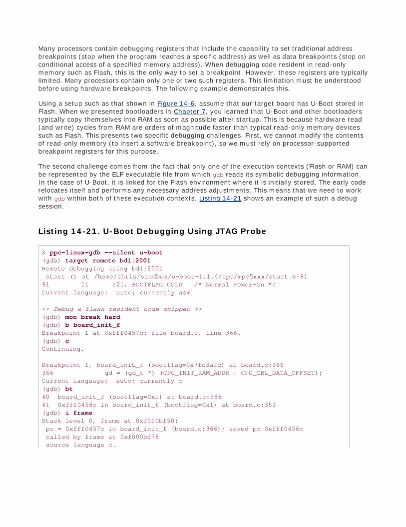
Many processors contain debugging registers that include the capability to set traditional addressbreakpoints (stop when the program reaches a specific address) as well as data breakpoints (stop onconditional access of a specified memory address). When debugging code resident in read-onlymemory such as Flash, this is the only way to set a breakpoint. However, these registers are typicallylimited. Many processors contain only one or two such registers. This limitation must be understoodbefore using hardware breakpoints. The following example demonstrates this.
Using a setup such as that shown in Figure 14-6, assume that our target board has U-Boot stored inFlash. When we presented bootloaders in Chapter 7, you learned that U-Boot and other bootloaderstypically copy themselves into RAM as soon as possible after startup. This is because hardware read(and write) cycles from RAM are orders of magnitude faster than typical read-only memory devicessuch as Flash. This presents two specific debugging challenges. First, we cannot modify the contentsof read-only memory (to insert a software breakpoint), so we must rely on processor-supportedbreakpoint registers for this purpose.
The second challenge comes from the fact that only one of the execution contexts (Flash or RAM) canbe represented by the ELF executable file from which gdb reads its symbolic debugging information.In the case of U-Boot, it is linked for the Flash environment where it is initially stored. The early coderelocates itself and performs any necessary address adjustments. This means that we need to workwith gdb within both of these execution contexts. Listing 14-21 shows an example of such a debugsession.
Listing 14-21. U-Boot Debugging Using JTAG Probe
$ ppc-linux-gdb --silent u-boot(gdb) target remote bdi:2001Remote debugging using bdi:2001_start () at /home/chris/sandbox/u-boot-1.1.4/cpu/mpc5xxx/start.S:9191 li r21, BOOTFLAG_COLD /* Normal Power-On */Current language: auto; currently asm
<< Debug a flash resident code snippet >>(gdb) mon break hard(gdb) b board_init_fBreakpoint 1 at 0xfff0457c: file board.c, line 366.(gdb) cContinuing.
Breakpoint 1, board_init_f (bootflag=0x7fc3afc) at board.c:366366 gd = (gd_t *) (CFG_INIT_RAM_ADDR + CFG_GBL_DATA_OFFSET);Current language: auto; currently c(gdb) bt#0 board_init_f (bootflag=0x1) at board.c:366#1 0xfff0456c in board_init_f (bootflag=0x1) at board.c:353(gdb) i frameStack level 0, frame at 0xf000bf50: pc = 0xfff0457c in board_init_f (board.c:366); saved pc 0xfff0456c called by frame at 0xf000bf78 source language c.

Arglist at 0xf000bf50, args: bootflag=0x1 Locals at 0xf000bf50, Previous frame's sp is 0x0
<< Now debug a memory resident code snippet after relocation >>(gdb) del 1(gdb) symbol-fileDiscard symbol table from '/home/chris/sandbox/u-boot-1.1.4-powerdna/u-boot'?(y or n) yNo symbol file now.(gdb) add-symbol-file u-boot 0x7fa8000add symbol table from file "u-boot" at .text_addr = 0x7fa8000(y or n) yReading symbols from u-boot...done.(gdb) b board_init_rBreakpoint 2 at 0x7fac6c0: file board.c, line 608.(gdb) cContinuing.Breakpoint 2, board_init_r (id=0x7f85f84, dest_addr=0x7f85f84) at board.c:608608 gd = id; /* initialize RAM version of global data */(gdb) i frameStack level 0, frame at 0x7f85f38: pc = 0x7fac6c0 in board_init_r (board.c:608); saved pc 0x7fac6b0 called by frame at 0x7f85f68 source language c. Arglist at 0x7f85f38, args: id=0x7f85f84, dest_addr=0x7f85f84 Locals at 0x7f85f38, Previous frame's sp is 0x0(gdb) mon break soft(gdb)
Study this example carefully. Some subtleties are definitely worth taking the time to understand.First, we connect to the Abatron BDI-2000 using the target remote command. The IP address in thiscase is that of the Abatron unit, represented by the symbolic name bdi.[10] The Abatron BDI-2000uses port 2001 for its remote gdb protocol connection.
[10] An entry in the host system's /etc/hosts file enables the symbolic IP address reference.
Next we issue a command to the BDI-2000 using the gdb mon command. The mon command tells gdbto pass the rest of the command directly to the remote hardware device. Therefore, mon break hardsets the BDI-2000 into hardware breakpoint mode.
We then set a hardware breakpoint at board_init_f. This is a routine that executes while still runningout of Flash memory at address 0xfff0457c. After the breakpoint is defined, we issue the continue ccommand to resume execution. Immediately, the breakpoint at board_init_f is encountered, and weare free to do the usual debugging activities, including stepping through code and examining data.You can see that we have issued the bt command to examine the stack backtrace and the i framecommand to examine the details of the current stack frame.
Now we continue execution again, but this time we know that U-Boot copies itself to RAM andresumes execution from its copy in RAM. So we need to change the debugging context while keepingthe debugging session alive. To accomplish this, we discard the current symbol table (symbol-file

command with no arguments) and load in the same symbol file again using the add-symbol-filecommand. This time, we instruct gdb to offset the symbol table to match where U-Boot has relocateditself to memory. This ensures that our source code and symbolic debugging information match theactual memory resident image.
After the new symbol table is loaded, we can add a breakpoint to a location that we know will residein RAM when it is executed. This is where one of the subtle complications is exposed. Because weknow that U-Boot is currently running in Flash but is about to move itself to RAM and jump to itsRAM-based copy, we must still use a hardware breakpoint. Consider what happens at this point if weuse a software breakpoint. gdb dutifully writes the breakpoint opcode into the specified memorylocation, but U-Boot overwrites it when it copies itself to RAM. The net result is that the breakpoint isnever hit, and we begin to suspect that our tools are broken. After U-Boot has entered the RAM copyand our symbol table has been updated to reflect the RAM-based addresses, we are free to use RAM-based breakpoints. This is reflected by the last command in Listing 14-21 setting the Abatron unitback to soft breakpoint mode.
Why do we care about using hardware versus software breakpoints? If we had unlimited hardwarebreakpoint registers, we wouldn't. But this is never the case. Here is what it looks like when you runout of processor-supported hardware breakpoint registers during a debug session:
(gdb) b flash_initBreakpoint 3 at 0x7fbebe0: file flash.c, line 70.(gdb) cContinuing.warning: Cannot insert breakpoint 3:Error accessing memory address 0x7fbebe0: Unknown error 4294967295.
Because we are debugging remotely, we aren't told about the resource constraint until we try toresume after entering additional breakpoints. This is because of the way gdb handles breakpoints.When a breakpoint is hit, gdb restores all the breakpoints with the original opcodes for that particularmemory location. When it resumes execution, it restores the breakpoint opcodes at the specifiedlocations. You can observe this behavior by enabling gdb's remote debug mode:
(gdb) set debug remote 1
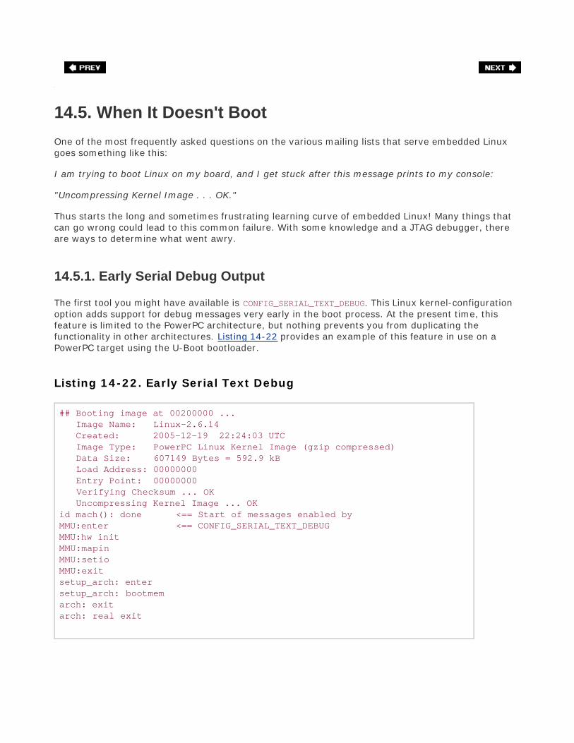
14.5. When It Doesn't Boot
One of the most frequently asked questions on the various mailing lists that serve embedded Linuxgoes something like this:
I am trying to boot Linux on my board, and I get stuck after this message prints to my console:
"Uncompressing Kernel Image . . . OK."
Thus starts the long and sometimes frustrating learning curve of embedded Linux! Many things thatcan go wrong could lead to this common failure. With some knowledge and a JTAG debugger, thereare ways to determine what went awry.
14.5.1. Early Serial Debug Output
The first tool you might have available is CONFIG_SERIAL_TEXT_DEBUG. This Linux kernel-configurationoption adds support for debug messages very early in the boot process. At the present time, thisfeature is limited to the PowerPC architecture, but nothing prevents you from duplicating thefunctionality in other architectures. Listing 14-22 provides an example of this feature in use on aPowerPC target using the U-Boot bootloader.
Listing 14-22. Early Serial Text Debug
## Booting image at 00200000 ... Image Name: Linux-2.6.14 Created: 2005-12-19 22:24:03 UTC Image Type: PowerPC Linux Kernel Image (gzip compressed) Data Size: 607149 Bytes = 592.9 kB Load Address: 00000000 Entry Point: 00000000 Verifying Checksum ... OK Uncompressing Kernel Image ... OKid mach(): done <== Start of messages enabled byMMU:enter <== CONFIG_SERIAL_TEXT_DEBUGMMU:hw initMMU:mapinMMU:setioMMU:exitsetup_arch: entersetup_arch: bootmemarch: exitarch: real exit

Using this feature, you can often tell where your board is getting stuck during the boot process. Ofcourse, you can add your own early debug messages in other places in the kernel. Here is anexample of its usage found in .../arch/ppc/mm/init.c:
/* Map in all of RAM starting at KERNELBASE */ if (ppc_md.progress) ppc_md.progress("MMU:mapin", 0x301); mapin_ram();
The AMCC Yosemite platform is an excellent example of this infrastructure. Consult the following filesin the Linux source tree[11] for details of how this debugging system is implemented:
[11] All these filenames are unique, so they can be found without full pathname references.
File Function Purpose
gen550_dbg.c gen550_init Serial port setup, called by yosemite.c platform-initialization file
gen550_dbg.c gen550_progress Low-level serial output routine
ibm44x_common.c ibm44x_platform_init Binds platform-specific progress routine to genericppc machine-dependent infrastructure
14.5.2. Dumping the printk Log Buffer
When we discussed printk debugging in Section 14.3.6, we pointed out some of the limitations of thismethod. printk itself is a very robust implementation. One of its shortcomings is that you can't seeany printk messages until later in the boot sequence when the console device has been initialized.Very often, when your board hangs on boot, quite a few messages are stuck in the printk buffer. Ifyou know where to find them, you can often pinpoint the exact problem that is causing the boot tohang. Indeed, many times you will discover that the kernel has encountered an error that led to a callto panic(). The output from panic() has likely been dumped into the printk buffer, and you canoften pinpoint the exact line of offending code.
This is best accomplished with a JTAG debugger, but it is still possible to use a bootloader and itsmemory dump capability to display the contents of the printk buffer after a reset. Some corruptionof memory contents might occur as a result of the reset, but log buffer text is usually very readable.
The actual buffer where printk stores its message text is declared in the printk source file.../kernel/printk.c.
static char __log_buf[__LOG_BUF_LEN];
We can easily determine the linked location of this buffer from the Linux kernel map file System.map.
$ grep __log_buf System.map c022e5a4 b __log_buf

Now if the system happens to hang upon booting, right after displaying the "Uncompressing KernelImage . . . OK" message, reboot and use the bootloader to examine the buffer. Because therelationship between kernel virtual memory and physical memory is fixed and constant on a givenarchitecture, we can do a simple conversion. The address of __log_buf shown earlier is a kernelvirtual address; we must convert it to a physical address. On this particular PowerPC architecture,that conversion is a simple subtraction of the constant KERNELBASE address, 0xc0000000. This is wherewe probe in memory to read the contents, if any, of the printk log buffer.
Listing 14-23 is an example of the listing as displayed by the U-Boot memory dump command.
Listing 14-23. Dump of Raw printk Log Buffer
=> md 22e5a40022e5a4: 3c353e4c 696e7578 20766572 73696f6e <5>Linux version0022e5b4: 20322e36 2e313320 28636872 6973406a 2.6.13 (chris@0022e5c4: 756e696f 72292028 67636320 76657273 junior) (gcc0022e5d4: 696f6e20 332e342e 3320284d 6f6e7461 version 3.4.3 (Monta0022e5e4: 56697374 6120332e 342e332d 32352e30 Vista 3.4.3-25.00022e5f4: 2e37302e 30353031 39363120 32303035 .70.0501961 20050022e604: 2d31322d 31382929 20233131 20547565 -12-18)) #11 Tue0022e614: 20466562 20313420 32313a30 353a3036 Feb 14 21:05:060022e624: 20455354 20323030 360a3c34 3e414d43 EST 2006.<4>AMC0022e634: 4320506f 77657250 43203434 30455020 C PowerPC 440EP0022e644: 596f7365 6d697465 20506c61 74666f72 Yosemite Platform.0022e654: 6d0a3c37 3e4f6e20 6e6f6465 20302074 <7>On node 00022e664: 6f74616c 70616765 733a2036 35353336 totalpages: 655360022e674: 0a3c373e 2020444d 41207a6f 6e653a20 .<7> DMA zone:0022e684: 36353533 36207061 6765732c 204c4946 65536 pages, LIF0022e694: 4f206261 7463683a 33310a3c 373e2020 O batch:31.<7>=>0022e6a4: 4e6f726d 616c207a 6f6e653a 20302070 Normal zone: 00022e6b4: 61676573 2c204c49 464f2062 61746368 pages, LIFO batch0022e6c4: 3a310a3c 373e2020 48696768 4d656d20 :1.<7> HighMemzone:0022e6d4: 7a6f6e65 3a203020 70616765 732c204c 0 pages,0022e6e4: 49464f20 62617463 683a310a 3c343e42 LIFO batch:1.<4>0022e6f4: 75696c74 2031207a 6f6e656c 69737473 Built 1 zonelists0022e704: 0a3c353e 4b65726e 656c2063 6f6d6d61 .<5>Kernel command0022e714: 6e64206c 696e653a 20636f6e 736f6c65 line: console0022e724: 3d747479 53302c31 31353230 3020726f =ttyS0,1152000022e734: 6f743d2f 6465762f 6e667320 72772069 root=/dev/nfs rw0022e744: 703d6468 63700a3c 343e5049 44206861 ip=dhcp.<4>PID0022e754: 73682074 61626c65 20656e74 72696573 hash table entries0022e764: 3a203230 34382028 6f726465 723a2031 : 2048 (order:0022e774: 312c2033 32373638 20627974 6573290a 11, 32768 bytes).0022e784: 00000000 00000000 00000000 00000000 ................0022e794: 00000000 00000000 00000000 00000000 ................=>

It's not very pretty to read, but the data is there. We can see in this particular example that thekernel crashed someplace after initializing the PID hash table entries. With some additional use ofprintk messages, we can begin to close in on the actual source of the crash.
As shown in this example, this is a technique that can be used with no additional tools. You can seethe importance of some kind of early serial port output during boot if you are working on a new boardport.
14.5.3. KGDB on Panic
If KGDB is enabled, the kernel attempts to pass control back to KGDB upon error exceptions. In somecases, the error itself will be readily apparent. To use this feature, a connection must already beestablished between KGDB and gdb. When the exception condition occurs, KGDB emits a Stop Replypacket to gdb, indicating the reason for the trap into the debug handler, as well as the address wherethe trap condition occurred. Listing 14-24 illustrates the sequence.
Listing 14-24. Trapping Crash on Panic Using KGDB
$ ppc-_4xx-gdb --silent vmlinux(gdb) target remote /dev/ttyS0Remote debugging using /dev/ttyS0Malformed response to offset query, qOffsets(gdb) target remote /dev/ttyS0Remote debugging using /dev/ttyS0breakinst () at arch/ppc/kernel/ppc-stub.c:825825 }(gdb) cContinuing.<< KGDB gains control from panic() on crash >>Program received signal SIGSEGV, Segmentation fault.0xc0215d6c in pcibios_init () at arch/ppc/kernel/pci.c:12631263 *(int *)-1 = 0;(gdb) bt#0 0xc0215d6c in pcibios_init () at arch/ppc/kernel/pci.c:1263#1 0xc020e728 in do_initcalls () at init/main.c:563#2 0xc020e7c4 in do_basic_setup () at init/main.c:605#3 0xc0001374 in init (unused=0x20) at init/main.c:677#4 0xc00049d0 in kernel_thread ()Previous frame inner to this frame (corrupt stack?)(gdb)
The crash in this example was contrived by a simple write to an invalid memory location (all ones).We first establish a connection from gdb to KGDB and allow the kernel to continue to boot. Noticethat we didn't even bother to set breakpoints. When the crash occurs, we see the line of offendingcode and get a nice backtrace to help us determine its cause.


14.6. Chapter Summary
Linux kernel debugging presents many complexities, especially in a cross-developmentenvironment. Understanding how to navigate these complexities is the key to successful kerneldebugging.
KGDB is a very useful kernel-level gdb stub that enables direct symbolic source-level debugginginside the Linux kernel and device drivers. It uses the gdb remote protocol to communicate toyour host-based cross-gdb.
Understanding (and minimizing) compiler optimizations helps make sense of seemingly strangedebugger behavior when stepping through compiler-optimized code.
gdb supports user-defined commands, which can be very useful for automating tediousdebugging tasks such as iterating kernel linked lists and accessing complex variables.
Kernel-loadable modules present their own challenges to source-level debugging. The module'sinitialization routine can be debugged by placing a breakpoint in module.c at the call to module->init().
printk and the Magic SysReq key provide additional tools to help isolate problems during kerneldevelopment and debugging.
Hardware-assisted debugging via a JTAG probe enables debugging Flash or ROM resident codewhere other debugging methods can be cumbersome or otherwise impossible.
Enabling CONFIG_SERIAL_TEXT_DEBUG on architectures where this feature is supported is apowerful tool for debugging a new kernel port.
Examining the printk log_buf often leads to the cause of a silent kernel crash on boot.
KGDB passes control to gdb on a kernel panic, enabling you to examine a backtrace and isolatethe cause of the kernel panic.
14.6.1. Suggestions for Additional Reading
Linux Kernel Development, 2nd EditionRobert LoveNovell Press, 2005
The Linux Kernel PrimerClaudia Salzberg Rodriguez et al.Prentice Hall, 2005
"Using the GNU Compiler Collection"

Richard M. Stallman and the GCC Developer CommunityGNU Press, a division of Free Software Foundationhttp://gcc.gnu.org/onlinedocs/
KGDB Sourceforge home pagehttp://sourceforge.net/projects/KGDB
Debugging with GDBRichard Stallman, Roland Pesch, Stan Shebs, et al.Free Software Foundationwww.gnu.org/software/gdb/documentation/
Tool Interface StandardsDWARF Debugging Information Format SpecificationVersion 2.0TIS Committee, May 1995

Chapter 15. Debugging Embedded LinuxApplicationsIn this chapter
Target Debugging page 400
Remote (Cross) Debugging page 400
Debugging with Shared Libraries page 405
Debugging Multiple Tasks page 411
Additional Remote Debug Options page 417
Chapter Summary page 419
In the previous chapter, we explored the use of GDB for debugging kernel code and code resident inFlash, such as bootloader code. In this chapter, we continue our coverage of GDB for debuggingapplication code in user space. We extend our coverage of remote debugging and the tools andtechniques used for this peculiar debugging environment.

15.1. Target Debugging
We already explored several important debugging tools in Chapter 13, "Development Tools." straceand ltrace can be used to observe and characterize a process's behavior and often isolate problems.dmalloc can help isolate memory leaks and profile memory usage. ps and top are both useful forexamining the state of processes. These relatively small tools are designed to run directly on thetarget hardware.
Debugging Linux application code on an embedded system has its own unique challenges. Resourceson your embedded target are often limited. RAM and nonvolatile storage limitations might preventyou from running target-based development tools. You might not have an Ethernet port or otherhigh-speed connection. Your target embedded system might not have a graphical display, keyboard,or mouse.
This is where your cross-development tools and an NFS root mount environment can yield largedividends. Many tools, especially GDB, have been architected to execute on your development hostwhile actually debugging code on a remote target. GDB can be used to interactively debug yourtarget code or to perform a postmortem analysis of a core file generated by an application crash. Wecovered the details of application core dump analysis in Chapter 13.

15.2. Remote (Cross) Debugging
Cross-development tools were developed primarily to overcome the resource limitations of embeddedplatforms. A modest-size application compiled with symbolic debug information can easily exceedseveral megabytes. With cross-debugging, the heavy lifting can be done on your development host.When you invoke your cross-version of GDB on your development host, you pass it an ELF filecompiled with symbolic debug information. On your target, there is no reason you can't strip [1] theELF file of all unnecessary debugging info to keep the resulting image to its minimum size.
[1] Remember to use your cross-version of strip, for example ppc_82xx-strip.
We introduced the readelf utility in Chapter 13. In Chapter 14, "Kernel Debugging Techniques," weused it to examine the debug information in an ELF file compiled with symbolic debugginginformation. Listing 15-1 contains the output of readelf for a relatively small web server applicationcompiled for the ARM architecture.
Listing 15-1. ELF File Debug Info for Example Program
$ xscale_be-readelf -S websdemoThere are 39 section headers, starting at offset 0x3dfd0:
Section Headers:[Nr] Name Type Addr Off Size ES Flg Lk Inf Al[ 0] NULL 00000000 000000 000000 00 0 0 0[ 1] .interp PROGBITS 00008154 000154 000013 00 A 0 0 1[ 2] .note.ABI-tag NOTE 00008168 000168 000020 00 A 0 0 4[ 3] .note.numapolicy NOTE 00008188 000188 000074 00 A 0 0 4[ 4] .hash HASH 000081fc 0001fc 00022c 04 A 5 0 4[ 5] .dynsym DYNSYM 00008428 000428 000460 10 A 6 1 4[ 6] .dynstr STRTAB 00008888 000888 000211 00 A 0 0 1[ 7] .gnu.version VERSYM 00008a9a 000a9a 00008c 02 A 5 0 2[ 8] .gnu.version_r VERNEED 00008b28 000b28 000020 00 A 6 1 4[ 9] .rel.plt REL 00008b48 000b48 000218 08 A 5 11 4[10] .init PROGBITS 00008d60 000d60 000018 00 AX 0 0 4[11] .plt PROGBITS 00008d78 000d78 000338 04 AX 0 0 4[12] .text PROGBITS 000090b0 0010b0 019fe4 00 AX 0 0 4[13] .fini PROGBITS 00023094 01b094 000018 00 AX 0 0 4[14] .rodata PROGBITS 000230b0 01b0b0 0023d0 00 A 0 0 8[15] .ARM.extab PROGBITS 00025480 01d480 000000 00 A 0 0 1[16] .ARM.exidx ARM_EXIDX 00025480 01d480 000008 00 AL 12 0 4[17] .eh_frame_hdr PROGBITS 00025488 01d488 00002c 00 A 0 0 4[18] .eh_frame PROGBITS 000254b4 01d4b4 00007c 00 A 0 0 4[19] .init_array INIT_ARRAY 0002d530 01d530 000004 00 WA 0 0 4[20] .fini_array FINI_ARRAY 0002d534 01d534 000004 00 WA 0 0 4[21] .jcr PROGBITS 0002d538 01d538 000004 00 WA 0 0 4

[22] .dynamic DYNAMIC 0002d53c 01d53c 0000d0 08 WA 6 0 4[23] .got PROGBITS 0002d60c 01d60c 000118 04 WA 0 0 4[24] .data PROGBITS 0002d728 01d728 0003c0 00 WA 0 0 8[25] .bss NOBITS 0002dae8 01dae8 0001c8 00 WA 0 0 4[26] .comment PROGBITS 00000000 01dae8 000940 00 0 0 1[27] .debug_aranges PROGBITS 00000000 01e428 0004a0 00 0 0 8[28] .debug_pubnames PROGBITS 00000000 01e8c8 001aae 00 0 0 1[29] .debug_info PROGBITS 00000000 020376 013d27 00 0 0 1[30] .debug_abbrev PROGBITS 00000000 03409d 002ede 00 0 0 1[31] .debug_line PROGBITS 00000000 036f7b 0034a2 00 0 0 1[32] .debug_frame PROGBITS 00000000 03a420 003380 00 0 0 4[33] .debug_str PROGBITS 00000000 03d7a0 000679 00 0 0 1[34] .note.gnu.arm.ide NOTE 00000000 03de19 00001c 00 0 0 1[35] .debug_ranges PROGBITS 00000000 03de35 000018 00 0 0 1[36] .shstrtab STRTAB 00000000 03de4d 000183 00 0 0 1[37] .symtab SYMTAB 00000000 03e5e8 004bd0 10 38 773 4[38] .strtab STRTAB 00000000 0431b8 0021bf 00 0 0 1Key to Flags:W (write), A (alloc), X (execute), M (merge), S (strings)I (info), L (link order), G (group), x (unknown)O (extra OS processing required) o (OS specific), p (processor specific)$
You can see from Listing 15-1 that there are many sections containing debug information. There isalso a .comment section that contains more than 2KB (0x940) of information that is not necessary forthe application to function. The size of this example file, including debug information, is more than275KB.
$ ls -l websdemo-rwxrwxr-x 1 chris chris 283511 Nov 8 18:48 websdemo
If we strip this file using the strip utility, we can minimize its size to preserve resources on ourtarget system. Listing 15-2 shows the results.
Listing 15-2. Strip Target Application
$ xscale_be-strip -s -R .comment -o websdemo-stripped websdemo$ ls -l websdemo*-rwxrwxr-x 1 chris chris 283491 Apr 9 09:19 websdemo-rwxrwxr-x 1 chris chris 123156 Apr 9 09:21 websdemo-stripped$
Here we strip both the symbolic debug information and the .comment section from the executable file.We specify the name of the stripped binary using the -o command line switch. You can see that theresulting size of the stripped binary is less than half of its original size. Of course, for largerapplications, this space savings can be even more significant. A recent Linux kernel compiled with

debug information was larger than 18MB. After stripping as in Listing 15-2, the resulting binary wasslightly larger than 2MB!
For debugging in this fashion, you place the stripped version of the binary on your target system andkeep a local unstripped copy on your development workstation containing symbolic informationneeded for debugging. You use gdbserver on your target board to provide an interface back to yourdevelopment host where you run the full-blown version of GDB on your nonstripped binary.
15.2.1. gdbserver
Using gdbserver allows you to run GDB from a development workstation rather than on the targetembedded Linux platform. This configuration has obvious benefits. For starters, it is common thatyour development workstation has far more CPU power, memory, and hard-drive storage than theembedded platform. In addition, it is common for the source code for your application under debug toexist on the development workstation and not on the embedded platform.
gdbserver is a small program that runs on the target board and allows remote debugging of aprocess on the board. It is invoked on the target board specifying the program to be debugged, aswell as an IP address and port number on which it will listen for connection requests from GDB.Listing 15-3 shows the startup sequence on the target board.
Listing 15-3. Starting gdbserver on Target Board
$ gdbserver localhost:2001 websdemo-strippedProcess websdemo-stripped created; pid = 197Listening on port 2001
This particular example starts gdbserver configured to listen for an Ethernet TCP/IP connection onport 2001, ready to debug our stripped binary program called websdemo-stripped.
From our development workstation, we launch GDB, passing it the name of the binary executablecontaining symbolic debug information that we want to debug as an argument. After GDB starts up,we issue a command to connect to the remote target board. Listing 15-4 shows this sequence.
Listing 15-4. Starting Remote GDB Session

$ xscale_be-gdb -q websdemo(gdb) target remote 192.168.1.141:2001Remote debugging using 192.168.1.141:20010x40000790 in ?? ()(gdb) p main <<<< display address of main function$1 = {int (int, char **)} 0x12b68 <main>(gdb) b main <<<< Place breakpoint at main()Breakpoint 1 at 0x12b80: file main.c, line 72.(gdb)
The sequence in Listing 15-4 invokes cross-gdb on your development host. When GDB is running, weissue the gdb target remote command. This command causes GDB to initiate a TCP/IP connectionfrom your development workstation to your target board, with the indicated IP address on port 2001.When gdbserver accepts the connection request, it prints a line similar to this:
Remote debugging from host 192.168.0.10
Now GDB is connected to the target board's gdbserver process, ready to accept commands fromGDB. The rest of the session is exactly the same as if you were debugging an application locally. Thisis a powerful tool, allowing you to use the power of your development workstation for the debugsession, leaving only a small, relatively unobtrusive GDB stub and your program being debugged onthe target board. In case you were wondering, gdbserver for this particular ARM target is only 54KB.
root@coyote:~# ls -l /usr/bin/gdbserver-rwxr-xr-x 1 root root 54344 Jul 23 2005 /usr/bin/gdbserver
There is one caveat, and it is the subject of a frequently asked question (FAQ) on many mailing lists.You must be using a GDB on your development host that was configured as a cross-debugger. It is abinary program that runs on your development workstation but understands binary executableimages compiled for another architecture. This is an important and frequently overlooked fact. Youcannot debug a PowerPC target with a native GDB such as that found in a typical Red Hat Linuxinstallation. You must have a GDB configured for your host and target combination.
When GDB is invoked, it displays a banner consisting of several lines of information and then displaysits compiled configuration. Listing 15-5 is an example of the GDB used for some examples in thisbook, which is part of an embedded Linux distribution provided by MontaVista Software configured forPowerPC cross-development.
Listing 15-5. Invocation of cross-gdb

$ ppc_82xx-gdbGNU gdb 6.0 (MontaVista 6.0-8.0.4.0300532 2003-12-24)Copyright 2003 Free Software Foundation, Inc.GDB is free software, covered by the GNU General Public License, andyou are welcome to change it and/or distribute copies of it undercertain conditions. Type "show copying" to see the conditions.There is absolutely no warranty for GDB. Type "show warranty" fordetails.This GDB was configured as "--host=i686-pc-linux-gnu--target=powerpc-hardhat-linux".(gdb)
Notice the last lines of this GDB startup message. This is the configuration compiled into this versionof GDB. It was compiled to execute on a Pentium (i686) PC host running GNU/Linux and to debugbinary programs compiled for a PowerPC processor running GNU/Linux. This is specified by the --host and --target variables displayed by the banner text, and is also a part of the configurationstring passed to ./configure when building GDB.

15.3. Debugging with Shared Libraries
Now that you understand how to invoke a remote debug session using GDB on the host andgdbserver on the target, we turn our attention to the complexities of shared libraries and debugsymbols. Unless your application is a statically linked executable (linked with the -static linkercommand line switch), many symbols in your application will reference code outside your application.Obvious examples include the use of standard C library routines such as fopen,printf,malloc, andmemcpy. Less obvious examples might include calls to application-specific functions, such asjack_transport_locate() (a routine from the JACK low-latency audio server), which calls a libraryfunction outside the standard C libraries.
To have symbols from these routines available, you must satisfy two requirements for GDB:
You must have debug versions of the libraries available.
GDB must know where to find them.
If you don't have debug versions of the libraries available, you can still debug your application; youjust won't have any debug information available for library routines called by your application. Oftenthis is perfectly acceptable, unless, of course, you are developing a shared library object as part ofyour embedded project.
Look back at Listing 15-4, where we invoked GDB on a remote target. After GDB connected via thetarget remote command, GDB issued a two-line response:
Remote debugging using 192.168.1.141:20010x40000790 in ?? ()
This confirms that GDB connected to our target at the indicated IP address and port. GDB thenreports the location of the program counter as 0x40000790. Why do we get question marks insteadof a symbolic location? Because this is the Linux dynamic loader (ld-x.y.z.so), and on this particularplatform, we do not have debug symbols available for this shared library. How do we know this?
Recall our introduction of the /proc file system from Chapter 9, "File Systems." One of the moreuseful entries was the maps enTRy (see Listing 9-16, in Chapter 9) in the per-process directorystructure. We know the process ID (PID) of our target application from the gdbserver output inListing 15-3. Our process was assigned PID 197. Given that, we can see the memory segments in useright after process startup, as shown in Listing 15-6.
Listing 15-6. Initial Target Memory Segment Mapping

root@coyote:~# cat /proc/197/maps00008000-00026000 r-xp 00000000 00:0e 4852444 ./websdemo-stripped0002d000-0002e000 rw-p 0001d000 00:0e 4852444 ./websdemo-stripped40000000-40017000 r-xp 00000000 00:0a 4982583 /lib/ld-2.3.3.so4001e000-40020000 rw-p 00016000 00:0a 4982583 /lib/ld-2.3.3.sobedf9000-bee0e000 rwxp bedf9000 00:00 0 [stack]root@coyote:~#
Here we see the target websdemo-stripped application occupying two memory segments. The first isthe read-only executable segment at 0x8000, and the second is a read-write data segment at0x2d000. The third memory segment is the one of interest. It is the Linux dynamic linker'sexecutable code segment. Notice that it starts at address 0x40000000. If we investigate further, wecan confirm that GDB is actually sitting at the first line of code for the dynamic linker, before anycode from our own application has been executed. Using our cross version of readelf, we can confirmthe starting address of the linker as follows:
# xscale_be-readelf -S ld-2.3.3.so | grep \.text[ 9] .text PROGBITS 00000790 000790 012c6c 00 AX 0 0 16
From this data, we conclude that the address GDB reports on startup is the first instruction from ld-2.3.3.so, the Linux dynamic linker/loader. You can use this technique to get rough ideas of whereyour code is if you don't have symbolic debug information for a process or shared library.
Remember that we are executing this cross readelf command on our development host. Therefore,the ld-2.3.3.so file, itself an XScale binary object, must be accessible to your development host.Most typically, this file resides on your development host, and is a component of your embeddedLinux distribution installed on your host.
15.3.1. Shared Library Events in GDB
GDB can alert you to shared library events. This can be useful for understanding your application'sbehavior or the behavior of the Linux loader, or for setting breakpoints in shared library routines youwant to debug or step through. Listing 15-7 illustrates this technique. Normally, the complete path tothe library is displayed. This listing has been edited for better readability.
Listing 15-7. Stopping GDB on Shared Library Events

$ xscale_be-gdb -q websdemo(gdb) target remote 192.168.1.141:2001Remote debugging using 192.168.1.141:20010x40000790 in ?? ()(gdb) i shared <<<Display loaded shared libsNo shared libraries loaded at this time.(gdb) b main <<<Break at mainBreakpoint 1 at 0x12b80: file main.c, line 72.(gdb) cContinuing.
Breakpoint 1, main (argc=0x1, argv=0xbec7fdc4) at main.c:7272 int localvar = 9;(gdb) i sharedFrom To Syms Read Shared Object Library0x40033300 0x4010260c Yes /opt/mvl/.../lib/tls/libc.so.60x40000790 0x400133fc Yes /opt/mvl/.../lib/ld-linux.so.3(gdb) set stop-on-solib-events 1(gdb) cContinuing.Stopped due to shared library event(gdb) i sharedFrom To Syms Read Shared Object Library0x40033300 0x4010260c Yes /opt/mvl/.../lib/tls/libc.so.60x40000790 0x400133fc Yes /opt/mvl/.../lib/ld-linux.so.30x4012bad8 0x40132104 Yes /opt/mvl/.../libnss_files.so.2(gdb)
When the debug session is first started, of course, no shared libraries are loaded. You can see thiswith the first i shared command. This command displays the shared libraries that are currentlyloaded. Setting a breakpoint at our application's main() function, we see that two shared libraries arenow loaded. These are the Linux dynamic linker/loader and the standard C library component libc.
From here, we issue the set stop-on-solib-event command and continue program execution. Whenthe application tries to execute a function from another shared library, that library is loaded. In caseyou are wondering, the gethostbyname() function is encountered and causes the next shared objectload.
This example illustrates an important cross-development concept. The binary application (ELF image)running on the target contains information on the libraries it needs to resolve its external references.We can view this information easily using the ldd command introduced in Chapter 11, "BusyBox,"and detailed in Chapter 13. Listing 15-8 shows the output of ldd invoked from the target board.
Listing 15-8. ldd Executed on Target Board

root@coyote:/workspace# ldd websdemo libc.so.6 => /lib/tls/libc.so.6 (0x40020000) /lib/ld-linux.so.3 (0x40000000)root@coyote:/workspace#
Notice that the paths to the shared libraries on the target are absolute paths starting at /lib on theroot file system. But GDB running on your host development workstation cannot use these paths tofind the libraries. You should realize that to do so would result in your host GDB loading libraries fromthe wrong architecture. Your host is likely x86, whereas, in this example, the target is ARM XScale.
If you invoke your cross version of ldd, you will see the paths that were preconfigured into yourtoolchain. Your toolchain must have knowledge of where these files exist on your host developmentsystem.[2] Listing 15-9 illustrates this. Again, we have edited the listing for readability; long pathshave been abbreviated.
[2] It is certainly possible to pass these locations to your compiler, linker, and debugger for every invocation, but any good
embedded Linux distribution will configure these defaults into the toolchain as a convenience to the developer.
Listing 15-9. ldd Executed on Development Host
$ xscale_be-ldd websdemo libc.so.6 => /opt/mvl/.../xscale_be/target/lib/libc.so.6 (0xdead1000) ld-linux.so.3 => /opt/mvl/.../xscale_be/target/lib/ld-linux.so.3 (0xdead2000)$
Your cross toolchain should be preconfigured with these library locations. Not only does your hostGDB need to know where they are located, but, of course, your compiler and linker also need thisknowledge.[3] GDB can tell you where it is configured to look for these libraries using the showsolib-absolute-prefix command:
[3] Of course, your compiler also needs to know the location of target files such as architecture-specific system and library header
files.
(gdb) show solib-absolute-prefixPrefix for loading absolute shared library symbol files is"/opt/mvl/pro/devkit/arm/xscale_be/target".(gdb)
You can set or change where GDB searches for shared libraries using the GDB commands set solib-absolute-prefix and set solib-search-path. If you are developing your own shared library modulesor have custom library locations on your system, you can use solib-search-path to instruct GDBwhere to look for your libraries. For more details about these and other GDB commands, consult theonline GDB manual referenced at the end of this chapter in Section 15.6.1, "Suggestions forAdditional Reading."
One final note about ldd. You might have noticed the addresses from Listing 15-8 and 15-9associated with the libraries. ldd displays the load address for the start of these code segments as

they would be if the program were loaded by the Linux dynamic linker/loader. Executed on thetarget, the addresses in Listing 15-5 make perfect sense, and we can correlate these with the/proc/<pid>/maps listing of the running process on the target. Listing 15-10 displays the memorysegments for this target process after it is completely loaded and running.
Listing 15-10. Memory Segments from /proc/<pid>/maps on Target
root@coyote:~# cat /proc/197/maps00008000-00026000 r-xp 00000000 00:0e 4852444 /workspace/websdemo-stripped0002d000-0002e000 rw-p 0001d000 00:0e 4852444 /workspace/websdemo-stripped0002e000-0005e000 rwxp 0002e000 00:00 0 [heap]40000000-40017000 r-xp 00000000 00:0a 4982583 /lib/ld-2.3.3.so40017000-40019000 rw-p 40017000 00:00 04001e000-4001f000 r--p 00016000 00:0a 4982583 /lib/ld-2.3.3.so4001f000-40020000 rw-p 00017000 00:0a 4982583 /lib/ld-2.3.3.so40020000-4011d000 r-xp 00000000 00:0a 4982651 /lib/tls/libc-2.3.3.so4011d000-40120000 ---p 000fd000 00:0a 4982651 /lib/tls/libc-2.3.3.so40120000-40124000 rw-p 000f8000 00:0a 4982651 /lib/tls/libc-2.3.3.so40124000-40126000 r--p 000fc000 00:0a 4982651 /lib/tls/libc-2.3.3.so40126000-40128000 rw-p 000fe000 00:0a 4982651 /lib/tls/libc-2.3.3.so40128000-4012a000 rw-p 40128000 00:00 04012a000-40133000 r-xp 00000000 00:0a 4982652 /lib/tls/libnss_files-2.3.3.so40133000-4013a000 ---p 00009000 00:0a 4982652 /lib/tls/libnss_files-2.3.3.so4013a000-4013b000 r--p 00008000 00:0a 4982652 /lib/tls/libnss_files-2.3.3.so4013b000-4013c000 rw-p 00009000 00:0a 4982652 /lib/tls/libnss_files-2.3.3.sobecaa000-becbf000 rwxp becaa000 00:00 0 [stack]root@coyote:~#
Notice the correlation of the target ldd output from Listing 15-8 to the memory segments displayedin the /proc file system for this process. The start (beginning of .text segment) of the Linux loader is0x40000000 and the start of libc is at 0x40020000. These are the virtual addresses where theseportions of the application have been loaded, and are reported by the target invocation of ldd.However, the load addresses reported by the cross version of ldd in Listing 15-9 (0xdead1000 and0xdead2000) are there to remind you that these libraries cannot be loaded on your host system (theyare ARM architecture binaries), and the load addresses are simply placeholders.

15.4. Debugging Multiple Tasks
Generally the developer is presented with two different debugging scenarios when dealing withmultiple threads of execution. Processes can exist in their own address space or can share an addressspace (and other system resources) with other threads of execution. The former (independentprocesses not sharing common address space) must be debugged using separate independent debugsessions. Nothing prevents you from using gdbserver on multiple processes on your target system,and using a separate invocation of GDB on your development host to coordinate a debug session formultiple cooperating but independent processes.
15.4.1. Debugging Multiple Processes
When a process being debugged under GDB uses the fork() system call [4] to spawn a new process,GDB can take two courses of action. It can continue to control and debug the parent process, or itcan stop debugging the parent process and attach to the newly formed child process. You can controlthis behavior using the set follow-fork-mode command. The two modes are follow parent and followchild. The default behavior is for GDB to follow the parent. In this case, the child process executesimmediately upon a successful fork.
[4] We will use the term system call, but fork() in this context is actually the C library function which in turn calls the Linux
sys_fork() system call.
Listing 15-11 reproduces a snippet of a simple program that forks multiple processes from its main()routine.
Listing 15-11. Using fork() to Spawn a Child Process
... for( i=0; i<MAX_PROCESSES; i++ ) { /* Creating child process */ pid[i] = fork(); /* Parent gets non-zero PID */ if ( pid[i] == -1 ) { perror("fork failed"); exit(1); } if ( pid[i] == 0 ) { /* Indicates child's code path */ worker_process(); /* The forked process calls this */ } }
/* Parent's main control loop */ while ( 1 ) {... }

This simple loop creates MAX_THREADS new processes using the fork() system call. Each newlyspawned process executes a body of code defined by the function worker_process(). When run underGDB in the default mode, GDB detects the creation of the new threads of execution (processes) butremains attached to the parent's thread of execution. Listing 15-12 illustrates this GDB session.
Listing 15-12. GDB in follow-fork-mode = parent
(gdb) target remote 192.168.1.141:20010x40000790 in ?? ()(gdb) b mainBreakpoint 1 at 0x8888: file forker.c, line 104.(gdb) cContinuing.[New Thread 356][Switching to Thread 356]
Breakpoint 1, main (argc=0x1, argv=0xbe807dd4) at forker.c:104104 time(&start_time);(gdb) b worker_processBreakpoint 2 at 0x8784: file forker.c, line 45.(gdb) cContinuing.Detaching after fork from child process 357.Detaching after fork from child process 358.Detaching after fork from child process 359.Detaching after fork from child process 360.Detaching after fork from child process 361.Detaching after fork from child process 362.Detaching after fork from child process 363.Detaching after fork from child process 364.
Notice that eight child processes were spawned, with PID values from 357 to 364. The parent processwas instantiated with PID 356. When the breakpoint in main() was hit, we entered a breakpoint atthe worker_process() routine, which each child process executes upon fork(). Letting the programcontinue from main, we see each of the new processes spawned and detached by the debugger. Theynever hit the breakpoint because GDB is attached to the main process, which never executes theworker_process() routine.
If you need to debug each process, you must execute a separate independent GDB session andattach to the child process after it is forked(). The GDB documentation referenced at the end of thischapter outlines a useful technique to place a call to sleep() in the child process, giving you time toattach a debugger to the new process. Attaching to a new process is explained in Section 15.5.2,"Attaching to a Running Process."
If you simply need to follow the child process, set the follow-fork-mode to follow child before yourparent reaches the fork() system call. Listing 15-13 shows this.

Listing 15-13. GDB in follow-fork-mode = child
(gdb) target remote 192.168.1.141:20010x40000790 in ?? ()(gdb) set follow-fork-mode child(gdb) b worker_processBreakpoint 1 at 0x8784: file forker.c, line 45.(gdb) cContinuing.[New Thread 401]Attaching after fork to child process 402.[New Thread 402][Switching to Thread 402]
Breakpoint 1, worker_process () at forker.c:4545 int my_pid = getpid();(gdb) cContinuing.
Here we see the parent process being instantiated as PID 401. When the first child is spawned by thefork() system call, GDB detaches silently from the parent thread of execution and attaches to thenewly spawned child process having PID 402. GDB is now in control of the first child process andhonors the breakpoint set at worker_process(). Notice, however, that the other child processesspawned by the code snippet from Listing 15-11 are not debugged and continue to run to their owncompletion.
In summary, using GDB in this fashion, you are limited to debugging a single process at a time. Youcan debug through the fork() system call, but you have to decide which thread of execution to followthrough the fork() call, either the parent or the child. As mentioned in the introduction to thissection, you can use multiple independent GDB sessions if you must debug more than onecooperating process at a time.
15.4.2. Debugging Multithreaded Applications
If your application uses the POSIX thread library for its threading functions, GDB has additionalcapabilities to handle concurrent debugging of a multithreaded application. The Native Posix ThreadLibrary (NPTL) has become the de facto standard thread library in use on Linux systems, includingembedded Linux systems. The rest of this discussion assumes that you are using this thread library.
For this section, we use a demonstration program that spawns a number of threads using thepthread_create() library function in a simple loop. After the threads are spawned, the main() routinesimply waits for keyboard input to terminate the application. Each thread displays a short messageon the screen and sleeps for a predetermined time. Listing 15-14 shows the startup sequence on thetarget board.
Listing 15-14. Target Threads Demo Startup

root@coyote:/workspace # gdbserver localhost:2001 ./tdemoProcess ./tdemo created; pid = 671Listening on port 2001Remote debugging from host 192.168.1.10 ^^^^^ Previous three lines displayed by gdbserver
tdemo main() entered: My pid is 671Starting worker thread 0Starting worker thread 1Starting worker thread 2Starting worker thread 3
As in our previous examples, gdbserver prepares the application for running and waits for aconnection from our host-based cross-gdb. When GDB connects, gdbserver reports the connectionwith the Remote debugging... message. Now we start GDB on the host and connect. Listing 15-15reproduces this half of the session.
Listing 15-15. Host GDB Connecting to Target Threads Demo
$ xscale_be-gdb -q tdemo(gdb) target remote 192.168.1.141:20010x40000790 in ?? ()(gdb) b tdemo.c:97Breakpoint 1 at 0x88ec: file tdemo.c, line 97.(gdb) cContinuing.[New Thread 1059][New Thread 1060][New Thread 1061][New Thread 1062][New Thread 1063][Switching to Thread 1059]
Breakpoint 1, main (argc=0x1, argv=0xbefffdd4) at tdemo.c:9898 int c = getchar();(gdb)
Here we connect to the target (resulting in the "Remote debugging..." message in Listing 15-14), seta breakpoint just past the loop where we spawned the new threads, and continue. When the newthread is created, GDB displays a notice along with the thread ID. Thread 1059 is the TDemoapplication, doing its work directly from the main() function. Threads 1060 through 1063 are the newthreads created from the call to pthread_create().
When GDB hits the breakpoint, it displays the message [Switching to Thread 1059], indicating thatthis was the thread of execution that encountered the breakpoint. It is the active thread for thedebugging session, referred to as the current thread in the GDB documentation.

GDB enables us to switch between threads and perform the usual debugging operations such assetting additional breakpoints, examining data, displaying a backtrace, and working with theindividual stack frames within the current thread. Listing 15-16 provides examples of theseoperations, continuing directly with our debugging session started in Listing 15-15.
Listing 15-16. GDB Operations on Threads
...(gdb) cContinuing. <<< Ctl-C to interrupt program executionProgram received signal SIGINT, Interrupt.0x400db9c0 in read () from /opt/mvl/.../lib/tls/libc.so.6(gdb) i threads 5 Thread 1063 0x400bc714 in nanosleep () from /opt/mvl/.../lib/tls/libc.so.6 4 Thread 1062 0x400bc714 in nanosleep () from /opt/mvl/.../lib/tls/libc.so.6 3 Thread 1061 0x400bc714 in nanosleep () from /opt/mvl/.../lib/tls/libc.so.6 2 Thread 1060 0x400bc714 in nanosleep () from /opt/mvl/.../lib/tls/libc.so.6* 1 Thread 1059 0x400db9c0 in read () from /opt/mvl/.../lib/tls/libc.so.6(gdb) thread 4 <<< Make Thread 4 the current thread[Switching to thread 4 (Thread 1062)]#0 0x400bc714 in nanosleep () from /opt/mvl/.../lib/tls/libc.so.6(gdb) bt#0 0x400bc714 in nanosleep () from /opt/mvl/.../lib/tls/libc.so.6#1 0x400bc4a4 in __sleep (seconds=0x0) at sleep.c:137#2 0x00008678 in go_to_sleep (duration=0x5) at tdemo.c:18#3 0x00008710 in worker_2_job (random=0x5) at tdemo.c:36#4 0x00008814 in worker_thread (threadargs=0x2) at tdemo.c:67#5 0x40025244 in start_thread (arg=0xfffffdfc) at pthread_create.c:261#6 0x400e8fa0 in clone () at../sysdeps/unix/sysv/linux/arm/clone.S:82#7 0x400e8fa0 in clone () at../sysdeps/unix/sysv/linux/arm/clone.S:82(gdb) frame 3#3 0x00008710 in worker_2_job (random=0x5) at tdemo.c:3636 go_to_sleep(random);
(gdb) l <<< Generate listing of where we are31 }3233 static void worker_2_job(int random)34 {35 printf("t2 sleeping for %d\n", random);36 go_to_sleep(random);

37 }3839 static void worker_3_job(int random)40 {(gdb)
A few points are worth mentioning. GDB assigns its own integer value to each thread and uses thesevalues to reference the individual threads. When a breakpoint is hit in a thread, all threads within theprocess are halted for examination. GDB marks the current thread with an asterisk (*). You can setunique breakpoints within each threadassuming, of course, that they exist in a unique context. If youset a breakpoint in a common portion of code where all threads execute, the thread that hits thebreakpoint first is arbitrary.
The GDB user documentation referenced at the end of this chapter contains more useful informationrelated to debugging in a multithreaded environment.
15.4.3. Debugging Bootloader/Flash Code
Debugging Flash resident code presents its own unique challenges. The most obvious limitation is theway in which GDB and gdbserver cooperate in setting target breakpoints. When we discussed theGDB remote serial protocol in Chapter 14, you learned how breakpoints are inserted into anapplication.[5] GDB replaces the opcode at the breakpoint location with an architecture-specificopcode that passes control to the debugger. However, in ROM or Flash, GDB cannot overwrite theopcode, so this method of setting breakpoints is useless.
[5] Refer back to Listing 14-5 in Chapter 14.
Most modern processors contain some number of debug registers that can be used to get around thislimitation. These capabilities must be supported by architecture-and processor-specific hardwareprobes or stubs. The most common technique for debugging Flash and ROM resident code is to useJTAG hardware probes. These probes support the setting of processor-specific hardware breakpoints.This topic was covered in detail in Chapter 14. Refer back to Section 14.4.2, "Debugging with a JTAGProbe," for details.

15.5. Additional Remote Debug Options
Sometimes you might want to use a serial port for remote debugging. For other tasks, you might findit useful to attach the debugger to a process that is already running. These simple but usefuloperations are detailed here.[6]
[6] Refer back to Listing 14-5 in Chapter 13
15.5.1. Debugging via Serial Port
Debugging via serial port is quite straightforward. Of course, you must have a serial port available onyour target that is not being used by another process, such as a serial console. The same limitationapplies to your host. A serial port must be available. If both of these conditions can be met, simplyreplace the IP:Port specification passed to gdbserver with a serial port specification. Use the sametechnique when connecting to your target from your host-based GDB.
On your target:
root@coyote:/workspace # gdbserver /dev/ttyS0 ./tdemoProcess ./tdemo created; pid = 698Remote debugging using /dev/ttyS0
From your host:
$ xscale_be-gdb -q tdemo(gdb) target remote /dev/ttyS1Remote debugging using /dev/ttyS10x40000790 in ?? ()
15.5.2. Attaching to a Running Process
It is often advantageous to connect to a process to examine its state while it is running instead ofkilling the process and starting it again. With gdbserver, it is trivial:
root@coyote:/workspace # ps ax | grep tdemo 1030 pts/0 Sl+ 0:00 ./tdemoroot@coyote:/workspace # gdbserver localhost:2001 --attach 1030Attached; pid = 1030Listening on port 2001
When you are finished examining the process under debug, you can issue the gdb detach command.This detaches the gdbserver from the application on the target and terminates the debug session.

The application continues where it left off. This is a very useful technique for examining a runningprogram. Be aware, though, that when you attach to the process, it halts, waiting for instructionsfrom you. It will not resume execution until instructed to do so, using either the continue commandor the detach command. Also note that you can use the detach command at almost any time to endthe debug session and leave the application running on the target.

15.6. Chapter Summary
Remote (cross) debugging enables symbolic debugging using host development workstationresources for the heavy lifting, preserving often scarce target resources.
gdbserver runs on the target system and acts as the glue between the cross-gdb running on adevelopment host and the process being debugged on the target.
GDB on the host typically uses IP connections via Ethernet to send and receive commands togdbserver running on the target. The GDB remote serial protocol is used between GDB andgdbserver.
GDB can halt on shared library events and can automatically load shared library symbols whenavailable. Your toolchain should be configured for the default paths on your cross-developmentsystem. Alternatively, you can use GDB commands to set the search paths for shared libraryobjects.
GDB can be used to debug multiple independent processes via multiple concurrent GDBsessions.
GDB can be configured to follow a forked process on a fork() system call. Its default mode is tocontinue to debug the parentthat is, the caller of fork().
GDB has features to facilitate debugging multithreaded applications written to POSIX threadAPIs. The current default Linux thread library is the Native Posix Threads Library (NPTL).
GDB supports attaching to and detaching from an already running process.
15.6.1. Suggestions for Additional Reading
GDB: The GNU Project DebuggerOnline Documentationhttp://sourceware.org/gdb/onlinedocs/
GDB Pocket ReferenceArnold RobbinsO'Reilly Media, 2005

Chapter 16. Porting LinuxIn this chapter
Linux Source Organization page 422
Custom Linux for Your Board page 424
Platform Initialization page 431
Putting It All Together page 439
Chapter Summary page 442
It is not difficult to port Linux to a new hardware platform. The Linux source tree contains ports fornumerous boards spanning more than 20 architectures and many more individual processors.Knowing where to start is often the hardest part.
This chapter covers the basics of porting Linux to a custom board providing support for basicEthernet and serial console operation. We examine the organization of the Linux source code from anarchitectural and platform perspective. We then delve into the early kernel initialization code tounderstand the mechanisms provided for platform initialization. Finally, we look at a typical portingeffort to a custom PowerPC hardware platform.

16.1. Linux Source Organization
Not too long ago, there were numerous homes[1] for the various versions of Linux. There was adedicated place for the PowerPC version of Linux, one for the ARM version, and so on. This wasn'tnecessarily by design, but by necessity. It took time to merge the various architecture infrastructureand features into the mainline kernel, and having a separate source tree meant quicker access to thelatest features in a given architecture.
[1] By "homes," we mean a public source code repository, such as a web server on the Internet.
The kernel developers have gone to great lengths to unify the Linux kernel source code to bringtogether the disparate architectures under one common source tree. With few exceptions, this is thecase today with the Linux 2.6 source. It is possible to download and compile working kernels for avariety of processors and industry-standard reference boards directly from www.kernel.org.
16.1.1. The Architecture Branch
In Chapter 4, "The Linux Kernel: A Different Perspective," we introduced the overall structure of theLinux kernel source tree. We spend the majority of this chapter examining the architecture-specificbranch of the Linux kernel sources. Listing 16-1 shows the contents of .../arch from a recent kernelsnapshot. As we pointed out in Chapter 4, the .../arch subdirectory is the second largest in terms ofsize, and in a recent Linux release, the largest in terms of file count (excluding the .../includedirectory). Only the .../drivers subdirectory is larger in size.
Listing 16-1. Linux Kernel .../arch Directory Listing
[chris@pluto linux]$ ls ./archalpha cris i386 m68k parisc s390 sparc v850arm frv ia64 m68knommu ppc sh sparc64 x86_64arm26 h8300 m32r mips ppc64 sh64 um xtensa
From this listing, you can see support for 24 separate architectures within the Linux kernel. We referto each as an architecture branch to facilitate our discussions.
Each architecture branch has some common components. For example, each top-level architecturebranch contains a Kconfig file. You will recall from Chapter 4 that Kconfig drives the kernelconfiguration utility. Of course, each top-level architecture branch also has a corresponding makefile.All the top-level architectures contain a kernel subdirectory because a number of kernel features arearchitecture dependent. All but two contain an mm subdirectory. This is where the architecture-dependent memory management code is found.
Many top-level architecture branches contain a boot subdirectory, which is used to build (through its

own makefile) a specific bootable target for that architecture. Many also contain mach-*subdirectories. These are used to hold code for specific machines or hardware platforms. Anothersubdirectory that appears frequently in the architecture branch is configs. This subdirectory exists formany of the more popular architectures and contains default configurations for each supportedhardware platform.
Throughout the rest of this chapter, we focus our discussion and examples on the PowerPCarchitecture. It is one of the most popular, with support for many processors and boards. Listing 16-2shows the contents of the configs directory for the .../arch/ppc PowerPC branch of a recent Linuxkernel release.
Listing 16-2. PowerPC configs Directory Contents
[chris@pluto linux]$ ls ./arch/ppc/configs/ads8272_defconfig IVMS8_defconfig prpmc750_defconfigapus_defconfig katana_defconfig prpmc800_defconfigbamboo_defconfig lite5200_defconfig radstone_defconfigbseip_defconfig lopec_defconfig redwood5_defconfigbubinga_defconfig luan_defconfig redwood6_defconfigchestnut_defconfig mbx_defconfig rpx8260_defconfigcommon_defconfig mpc834x_sys_defconfig rpxcllf_defconfigcpci405_defconfig mpc8540_ads_defconfig rpxlite_defconfigcpci690_defconfig mpc8548_cds_defconfig sandpoint_defconfigebony_defconfig mpc8555_cds_defconfig spruce_defconfigep405_defconfig mpc8560_ads_defconfig stx_gp3_defconfigest8260_defconfig mpc86x_ads_defconfig sycamore_defconfigev64260_defconfig mpc885ads_defconfig TQM823L_defconfigev64360_defconfig mvme5100_defconfig TQM8260_defconfigFADS_defconfig ocotea_defconfig TQM850L_defconfiggemini_defconfig pmac_defconfig TQM860L_defconfighdpu_defconfig power3_defconfig walnut_defconfigibmchrp_defconfig pplus_defconfig
Each one of these entries in the configs directory of the PowerPC architecture branch represents aspecific port to a hardware platform. For example, walnut_defconfig defines the default configurationfor the AMCC Walnut PPC405 evaluation platform. The mpc8540_ads_defconfig file represents thedefault configuration for the Freescale MPC8540 ADS evaluation board. As described in Chapter 4, tobuild a kernel for these reference platforms you first configure your kernel source tree with theseconfiguration defaults, as follows:
$ make ARCH=ppc CROSS_COMPILE=ppc_85xx- mpc8540_ads_defconfig
This invocation of make (from the top-level Linux directory) configures the kernel source tree with adefault configuration for the Freescale MPC8540 ADS evaluation board.
One aspect of the Linux kernel source tree that has not achieved significant unification is the way inwhich each architecture handles platform-specific files. In the PowerPC branch, you find a platformsdirectory that contains platform-specific code. Looking through this directory, you will see many

source files named after the respective hardware platform. There are also a few subdirectories under.../arch/ppc/platforms for specific PowerPC variants.
In contrast, the ARM branch contains a series of mach-* directories, each representing a specifichardware platform, while the MIPS branch has a set of subdirectories named for a specific platform.

16.2. Custom Linux for Your Board
When we ported U-Boot to a new hardware platform in Chapter 7, "Bootloaders," we found theconfiguration that most closely matched our new board and borrowed from that port. We use asimilar technique to port Linux to our new board. We assume that the chosen CPU is alreadysupported in the kernel. Porting to a new CPU is significantly more challenging and beyond the scopeof this book.
We have chosen to port Linux to a custom controller board based on the Freescale MPC5200 32-bitembedded PowerPC processor. Looking through the default configurations from a recent Linuxrelease (as depicted in Listing 16-2), we find one that contains the MPC5200 CPU. Because it appearsthat this is the only configuration that supports this processor, we use it as our baseline.
The hardware platform that we use for this exercise was supplied courtesy of United ElectronicIndustries. The board is called the PowerDNA Controller. It has a simple block diagram, containingonboard Flash memory, dynamic RAM, a serial port, and a variety of I/O devices, mostly integratedinto the MPC5200 processor. Figure 16-1 is the block diagram of the PowerDNA Controller.
Figure 16-1. UEI PowerDNA Controller board

16.2.1. Prerequisites and Assumptions
The Linux kernel makes some fundamental assumptions when it is passed control from a bootloader.Most important among them is that the bootloader must have initialized the DRAM controller. Linuxdoes not participate in chip-level SDRAM controller setup. Linux assumes that system RAM is presentand fully functional. The PowerDNA Controller we are targeting contains the U-Boot bootloader, whichhas initialized the CPU, DRAM, and other related hardware required for minimal system operation.
The bootloader should also initialize the system memory map. This is usually done via a set ofprocessor registers that define what chip select signals are active within a given memory addressrange. Chapter 3 in the Freescale MPC5200 User's Guide describes the registers used for this task.
The bootloader might have additional hardware-related initialization tasks. On some boards, thekernel assumes that the serial port is configured. This makes it possible to display early kernel bootmessages to the serial port, long before the kernel's own serial driver has been installed. Somearchitectures and hardware platforms contain functions such as *_serial_putc(), which can sendstrings to a serial port that has been preconfigured by the bootloader or by some simple early kernelsetup code. You can find examples of this in the PowerPC architecture branch using grep andsearching for CONFIG_SERIAL_TEXT_DEBUG.
In summary, the fundamental prerequisite for porting Linux to our new board is that a bootloader hasbeen ported and installed on our board, and any board-specific low-level hardware initialization hasbeen completed. It is not necessary to initialize devices for which Linux has direct device driversupport, such as Ethernet controllers or I2C controllers; the kernel handles these.
It is a good idea to configure and build your Linux kernel for the board closest to your own. Thisprovides you with a known good starting pointa Linux kernel source tree configured for your boardthat compiles without error. Recall from Chapter 5, "Kernel Initialization," the command to compile aLinux 2.6 kernel:
$ make ARCH=ppc CROSS_COMPILE=ppc_82xx- uImage
This command line results in a Linux bootable image compatible with the U-Boot bootloader. TheuImage target specifies this.
16.2.2. Customizing Kernel Initialization
Now that we have a baseline kernel source tree from which to start, let's determine where to begincustomizing for our particular board. We discovered that for the PowerPC architecture, the board-specific files reside in a directory called .../arch/ppc/platforms. Of course, this is not strictlynecessary, but if you ever intend to submit your patches to the Linux kernel development communityfor consideration, proper form and consistency matter!
We find in the platforms directory a file called lite5200.c. It's a fairly simple file, containing twodata structures and five functions. Listing 16-3 presents the functions from this file.
Listing 16-3. Functions from 5200 Platform File

lite5200_show_cpuinfo() /* Prints user specified text string */lite5200_map_irq() /* Sets h/w specific INT logic routing */lite5200_setup_cpu() /* CPU specific initialization */lite5200_setup_arch() /* Arch. specific initialization */platform_init() /* Machine or board specific init */
Let's look at how these functions are used. We briefly examined the low-level kernel initialization inChapter 5. Here we look at the details for a particular architecture. Details differ betweenarchitectures, but when you can navigate one, the others will be easier to learn.
From Chapter 5, we saw the early flow of control on power-up. The bootloader passed control to thekernel's bootstrap loader, which then passed control to the Linux kernel via the kernel's head.omodule. Here the platform-specific initialization begins. Listing 16-4 reproduces the pertinent linesfrom .../arch/ppc/kernel/head.S.
Listing 16-4. Calling Early Machine Initialization
.../* * Do early bootinfo parsing, platform-specific initialization, * and set up the MMU. */ mr r3,r31 mr r4,r30 mr r5,r29 mr r6,r28 mr r7,r27 bl machine_init bl MMU_init ...
Here you can see the assembly language call to machine_init. Of particular significance is the setupof the registers r3 through r7. These registers are expected to contain well-known values, which youwill see momentarily. They were stored away very early in the boot sequence to the PowerPCgeneral-purpose registers r27 tHRough r31. Here they are reloaded from these stored values.
The machine_init() function is defined in a C file called setup.c, in the same architecture-specifickernel directory: .../arch/ppc/kernel/setup.c. The start of this routine is reproduced here in Listing16-5.
Listing 16-5. Function machine_init() in setup.c

void __initmachine_init(unsigned long r3, unsigned long r4, unsigned long r5, unsigned long r6, unsigned long r7){#ifdef CONFIG_CMDLINE strlcpy(cmd_line, CONFIG_CMDLINE, sizeof(cmd_line));#endif /* CONFIG_CMDLINE */
#ifdef CONFIG_6xx ppc_md.power_save = ppc6xx_idle;#endif#ifdef CONFIG_POWER4 ppc_md.power_save = power4_idle;#endif
platform_init(r3, r4, r5, r6, r7);
if (ppc_md.progress) ppc_md.progress("id mach(): done", 0x200);}
There is some very useful knowledge in this simple function. First, notice that the parameters tomachine_init() represent the PowerPC general-purpose registers r3 through r7.[2] You saw that theywere initialized just before the machine language call to machine_init. As you can see from Listing16-5, these register values are passed unmodified to platform_init(). We need to modify thisfunction for our platform. (We have more to say about that in a moment.)
[2] By convention, parameters in C are passed in these PowerPC registers.
Listing 16-5 also contains some machine-specific calls for power-management functions. If yourkernel is configured for PowerPC 6xx support (CONFIG_6xx defined in your .config file), a pointer to amachine-specific power-management function (ppc6xx_idle) is stored in a structure. Similarly, if yourkernel is configured for a PowerPC G5 core (CONFIG_POWER4), a pointer to its machine-specific power-management routine is stored in the same structure member. This structure is described in Section16.3.3, "Machine-Dependent Calls."
16.2.3. Static Kernel Command Line
One of the more interesting operations in the machine_init() function reproduced in Listing 16-5 isto store the default kernel command line. This operation is enabled if CONFIG_CMDLINE is enabled inyour kernel configuration. On some platforms, the bootloader does not supply the kernel commandline. In these cases, the kernel command line can be statically compiled into the kernel. Figure 16-2illustrates the configuration options for this.

Figure 16-2. Default kernel command line
[View full size image]
Enable "Default bootloader kernel arguments" in the configuration in Figure 16-2 and edit the "Initialkernel command string" as shown. This results in a set of entries in the .config file, as shown inListing 16-6.
Listing 16-6. Configuration for Default Kernel Command Line
...CONFIG_CMDLINE_BOOL=yCONFIG_CMDLINE="console=ttyS0 root=/dev/ram0 rw"...
The ellipses in Listing 16-6 indicate that we have taken only a small snippet of the .config file. Whenthese configuration symbols are processed by the kernel build system, they become entries in the.../include/linux/autoconf.h file, as detailed in Listing 16-7.
Listing 16-7. File autoconf.h Entries for Default Kernel Command Line
... #define CONFIG_CMDLINE_BOOL 1 #define CONFIG_CMDLINE "console=ttyS0 root=/dev/ram0 rw"...

Now referring back to Listing 16-5, we have the following line:
strlcpy(cmd_line, CONFIG_CMDLINE, sizeof(cmd_line));
You can see that this kernel-based string-copy function copies the string defined by CONFIG_CMDLINEinto a global kernel variable called cmd_line. This is important because many functions and devicedrivers might need to examine the kernel command line early in the boot sequence. The globalvariable cmd_line is hidden away at the start of the .data section, defined in the assembler file.../arch/ppc/kernel/head.S.
A subtle detail is worth mentioning here. Looking back at Listing 16-4, we see that the machine_initassembly language call is made before the call to MMU_init. That means that any code we are able torun from machine_init is executed in a context with limited support for accessing memory. Many oftoday's processors that contain an MMU cannot access any memory without some initial mapping viahardware registers in the processor.[3] Typically, a small amount of memory is made available atboot time to accommodate loading and decompressing the kernel and a ramdisk image. Trying toaccess code or data beyond these early limits will fail. Each architecture and platform might havedifferent early limits for accessing memory. Values on the order of 8 to 16MB are not untypical. Wemust remember that any code we execute from machine_init, including our platform initialization,takes place in this context. If you encounter data access errors (PowerPC DSI exception[4]) whiledebugging your new kernel port, you should immediately suspect that you have not properly mappedthe memory region your code is trying to access.
[3] The AMCC PPC405 is a perfect example of this. The interested reader is encouraged to examine the BAT registers in this
processor.
[4] Refer to the Programming Environments Manual referenced at the end of this chapter for details of the PowerPC DSI
exception.

16.3. Platform Initialization
Following is a quick review of the code flow during early initialization. Figure 16-3 shows the flow ofexecution from the bootloader or bootstrap loader to your platform-initialization code.
Figure 16-3. Platform initialization flow of control
The files head.S and setup.c are both found in the .../arch/ppc/kernel directory for the PowerPCarchitecture. Our custom platform-initialization file will be placed in the .../arch/ppc/platformsdirectory. In Figure 16-3, it is represented by the file myplat.c. We are now in a position to examinethe platform-specific initialization file in detail.
In Listing 16-3, we listed the functions in the lite5200.c platform-initialization file. Every functionexcept platform_init() is declared as static. Therefore, as shown in Figure 16-3, this is the entrypoint for the platform-initialization file. The rest of the functions in the file are referenced only fromwithin the file itself.
Let's examine the entry function platform_init(). Listing 16-8 reproduces the platform_init()function from the lite5200.c file.
Listing 16-8. Lite5200 platform_init Function
void __initplatform_init(unsigned long r3, unsigned long r4, unsigned long r5, unsigned long r6, unsigned long r7){ /* Generic MPC52xx platform initialization */ /* TODO Create one and move a max of stuff in it. Put this init in the syslib */

struct bi_record *bootinfo = find_bootinfo();
if (bootinfo) parse_bootinfo(bootinfo); else { /* Load the bd_t board info structure */ if (r3) memcpy((void*)&__res,(void*)(r3+KERNELBASE), sizeof(bd_t));
#ifdef CONFIG_BLK_DEV_INITRD /* Load the initrd */ if (r4) { initrd_start = r4 + KERNELBASE; initrd_end = r5 + KERNELBASE; }#endif
/* Load the command line */ if (r6) { *(char *)(r7+KERNELBASE) = 0; strcpy(cmd_line, (char *)(r6+KERNELBASE)); } }
/* PPC Sys identification */ identify_ppc_sys_by_id(mfspr(SPRN_SVR));
/* BAT setup */ mpc52xx_set_bat();
/* No ISA bus by default */ isa_io_base = 0; isa_mem_base = 0;
/* Powersave */ /* This is provided as an example on how to do it. But you need to be aware that NAP disable bus snoop and that may be required for some devices to work properly, like USB ... */ /* powersave_nap = 1; */

/* Setup the ppc_md struct */ ppc_md.setup_arch = lite5200_setup_arch; ppc_md.show_cpuinfo = lite5200_show_cpuinfo; ppc_md.show_percpuinfo = NULL; ppc_md.init_IRQ = mpc52xx_init_irq; ppc_md.get_irq = mpc52xx_get_irq;
#ifdef CONFIG_PCI ppc_md.pci_map_irq = lite5200_map_irq;#endif
ppc_md.find_end_of_memory = mpc52xx_find_end_of_memory; ppc_md.setup_io_mappings = mpc52xx_map_io;
ppc_md.restart = mpc52xx_restart; ppc_md.power_off = mpc52xx_power_off; ppc_md.halt = mpc52xx_halt;
/* No time keeper on the LITE5200 */ ppc_md.time_init = NULL; ppc_md.get_rtc_time = NULL; ppc_md.set_rtc_time = NULL;
ppc_md.calibrate_decr = mpc52xx_calibrate_decr;#ifdef CONFIG_SERIAL_TEXT_DEBUG
ppc_md.progress = mpc52xx_progress;#endif}
This function contains much of the customizing that is required for this particular platform. It startsby searching for board-specific data supplied by the bootloader. We defer discussion of the details ofthis until Section 16.3.2, "Board Information Structure."
Following this, if your kernel is configured for an initial ramdisk (initrd),[5] the start and endaddresses of the ramdisk image are saved. Notice that they are passed in the PowerPC general-purpose registers r4 and r5 by convention. It is the bootloader's responsibility to pass the initrdaddresses in these registers. Later, the kernel will use these addresses to load the initrd image fromraw memory (where the bootloader placed it, or a nonvolatile Flash image) into an internal kernelramdisk structure.
[5] The initial ramdisk, or initrd, was introduced in Chapter 6.

Next we see code to store the kernel command line, whose address is passed into platform_init()via registers r6 and r7, marking the start and end addresses, respectively. This differs from themethod described earlier for storing a static kernel command line in one specific detail: this kernelcommand line was passed to platform_init() from the bootloader, as opposed to being compiledinto the kernel.
Copying the initrd and kernel command line is very straightforward. Basically, the registers passedin from the bootloader contain the memory addresses where these data structures reside. There isone minor subtlety, however. You may have already wondered about the purpose of the constantKERNELBASE. Understanding this is key to grasping one of the more complex parts of the bootsequence.
The addresses the bootloader provides are physical addresses. This means they are the realhardware addresses where the data resides in the memory chips. The bootloader typically operateswithout support for virtual memory. However, the kernel itself is statically linked to a well-known,user-configured base address. This address is KERNELBASE. (The value itself is not relevant to thediscussionit is user configurable but virtually never changed from its default value of 0xC0000000.)
This sets up an interesting situation in head.S. When the kernel is decompressed and relocated toRAM (usually to location 0), all of its code and data symbols are linked at the kernel's virtual address,KERNELBASE. This can be seen by examining the kernel symbol map file, produced during the kernelbuild process, System.map.[6] However, the execution context prior to enabling the MMU is such thatphysical addresses are real hardware addresses. This means that all the code prior to enabling theMMU and virtual memory mapping must be relocatable, and access to symbols must be fixed up. Thisinvolves adding an offset to the symbol's address to access it. An example will make this clear.
[6] We introduced the System.map file in Chapter 4.
16.3.1. Early Variable Access
Let's assume that a code segment very early in the boot process needs to access the variablecmd_lineso early that we're executing in 1:1 real to physical mapping. As pointed out earlier, thisvariable is defined in head.S and will end up in the .data section when the kernel is linked. From theLinux kernel's System.map file, you can find the linked addresses for cmd_line:
$ cat System.map | grep cmd_line c0115000 D cmd_line
If we were running in real = physical mode (MMU disabled) and accessed this variable using itssymbol, we would be trying to read or write to an address greater than 3GB. Most smaller embeddedsystems don't have any RAM in this region, and the results would be undefined or would result in acrash. Even if we had physical RAM at that address, it is unlikely that it would be mapped andaccessible this early in the boot process. So we have to adjust our reference to this variable to accessit.
Listing 16-9 reproduces a code snippet from head.S that does just that.
Listing 16-9. Variable Reference Fixup

relocate_kernel: addis r9,r26,klimit@ha /* fetch klimit */ lwz r25,klimit@l(r9) addis r25,r25,-KERNELBASE@h
This code snippet from the PowerPC head.S is a good example of the issue we are describing. Thevariable klimit represents the end of the kernel image. It is defined elsewhere as char *klimit.Therefore, it is a pointerit is an address that contains an address. In Listing 16-9, we fetch theaddress of klimit, sum it with a previously calculated offset that is passed in r26, and deposit theresulting value in register r9. Register r9 now contains the high-order 16 bits of the adjusted addressof klimit, with the low-order bits zeroed.[7] It was adjusted by the offset value previously calculatedand passed in register r26.
[7] For details of PPC assembly language syntax, see Section 16.5.1, "Suggestions for Additional Reading" at the end of this
chapter.
In the next line, the lwz instruction uses register r9 together with the offset of klimit (the lower 16bits of the klimit address) as an effective address from which to load register r25. (Remember,klimit is a pointer, and we are interested in the value that klimit points to.) Register r25 now holdsthe pointer that was stored in the variable klimit. In the final line of Listing 16-9, we subtract thekernel's linked base address (KERNELBASE) from r25 to adjust the pointer to our actual physicaladdress. In C, it would look like this:
unsigned int *tmp; /* represents r25 */ tmp = *klimit; tmp -= KERNELBASE;
In summary, we referenced a pointer stored in klimit and adjusted its value to our real (physical)address so we can use its contents. When the kernel enables the MMU and virtual addressing, we nolonger have to worry about thisthe kernel will be running at the address where it was linked,regardless of where in physical memory it is actually located.
16.3.2. Board Information Structure
Many bootloaders are used for PowerPC platforms, but there is still no unified way to pass in board-specific data such as serial port baud rate, memory size, and other low-level hardware parametersthat the bootloader has configured. The platform-initialization file from Listing 16-8 supports twodifferent methods, data stored as struct bi_record and data stored as struct bd_info.[8] Bothmethods provide similar results: hardware-specific data is passed from the bootloader to the kernelin these structures.
[8] Each method has its own roots. The struct bd_info originated in U-Boot, and struct bi_record was an attempt to unify
across all platforms. Both are supported by many platforms.
From Listing 16-8, here is the code snippet that saves the bootloader-supplied hardwareconfiguration:
struct bi_record *bootinfo = find_bootinfo();

if (bootinfo) parse_bootinfo(bootinfo); else { /* Load the bd_t board info structure */ if (r3) memcpy((void*)&__res,(void*)(r3+KERNELBASE), sizeof(bd_t));
First, we search for a special tag that identifies the data structure as a struct bi_record. If that isfound, the bootinfo pointer is set to the address of the start of the bootinfo records. From there, therecords are parsed and the hardware related data is gathered. This can be seen by inspecting.../arch/ppc/kernel/setup.c. Currently, bi_records can contain the kernel command line, the startand end address of the initrd image, the machine type, and the size of the memory. Of course, youcan extend this for your own requirements.
If no bi_record data is found, the PowerPC architecture expects this data in the form of U-Boot boardinformation structure, or bd_info. It is the bootloader's responsibility to construct this data structureand pass the address in register r3. Currently, many bits of hardware information are available in thebd_info structure, including information on DRAM, FLASH, SRAM, processor clock rates, busfrequencies, serial port baud rate setting, and more.
The bi_record structure can be examined in .../include/asm-ppc/bootinfo.h, and the bd_infostructure can be found in .../include/asm-ppc/ppcboot.h.
It is the responsibility of the platform-initialization routines to make use of any of the data that mightbe necessary to complete the hardware setup, or to communicate it to the kernel. For example,platform_init() sets up a pointer to a function whose name reveals its purpose. The code fromListing 16-8 is reproduced here:
ppc_md.find_end_of_memory = mpc52xx_find_end_of_memory;
Looking at the function mpc52xx_find_end_of_memory(), which is found in.../arch/ppc/syslib/mpc52xx_setup.c, we find the following:
u32 ramsize = __res.bi_memsize;
if (ramsize == 0) { ... /* Find it another way */ }
return ramsize;
The __res data structure above is the board information structure, whose address was passed to usfrom the bootloader in register r3 above. As you can see, the generic setup code stored the residualdata (as it is often called) passed in by the bootloader, but it's up to the machine or platform-specificcode to make use of it.

16.3.3. Machine-Dependent Calls
Many common routines that the kernel needs either for initialization or for operation are architectureand machine (CPU) dependent. From the platform_init() function reproduced in Listing 16-8, wesaw the following:
... /* Setup the ppc_md struct */ ppc_md.setup_arch = lite5200_setup_arch; ppc_md.show_cpuinfo = lite5200_show_cpuinfo; ppc_md.show_percpuinfo = NULL; ppc_md.init_IRQ = mpc52xx_init_irq; ppc_md.get_irq = mpc52xx_get_irq;
#ifdef CONFIG_PCI ppc_md.pci_map_irq = lite5200_map_irq;#endif
ppc_md.find_end_of_memory = mpc52xx_find_end_of_memory; ppc_md.setup_io_mappings = mpc52xx_map_io;
ppc_md.restart = mpc52xx_restart; ppc_md.power_off = mpc52xx_power_off; ppc_md.halt = mpc52xx_halt;...
Lines similar to these make up the rest of the platform_init() function. Here the bulk of theplatform-specific needs are communicated to the Linux kernel. The global variable ppc_md, of typestruct machdep_calls, provides the hooks to easily customize the Linux kernel for a PowerPCplatform. This variable is declared in .../arch/ppc/kernel/setup.c. Many places in the PowerPC-specific kernel branch call functions indirectly through this structure. For example, Listing 16-10reproduces a portion of .../arch/ppc/kernel/setup.c, which contains support for the restart, power-off, and halt functions:
Listing 16-10. Generic PowerPC Machine Functions

void machine_restart(char *cmd){#ifdef CONFIG_NVRAM nvram_sync();#endif ppc_md.restart(cmd);}
void machine_power_off(void){#ifdef CONFIG_NVRAM nvram_sync();#endif ppc_md.power_off();}
void machine_halt(void){#ifdef CONFIG_NVRAM nvram_sync();#endif ppc_md.halt();}
These functions are called via the ppc_md structure and contain the machine- or platform-specificvariants of these functions. You can see that some of these functions are machine specific and comefrom mpc52xx_* variants of the functions. Examples of these include mpc52xx_restart andmpc52xx_map_io. Others are specific to the hardware platform. Examples of platform-specific routinesinclude lite5200_map_irq and lite5200_setup_arch.

16.4. Putting It All Together
Now that we have a reference from which to proceed, we can create the necessary files and functionsfor our own custom board. We copy the Lite5200 platform files for our baseline and modify them forour custom PowerPC platform. We'll call our new platform PowerDNA. The steps we will perform forthis custom port are as follows:
1. Add a new configuration option to ...arch/ppc/Kconfig.
2. Copy lite5200.* to powerdna.* as a baseline.
3. Edit new powerdna.* files as appropriate for our platform.
4. Edit .../arch/ppc/Makefile to conditionally includepowerdna.o.
5. Compile, load, and debug!
You learned how to add a configuration option to Kconfig in Chapter 4. The configuration option forour new PowerDNA port is detailed in Listing 16-11.
Listing 16-11. Configuration Option for PowerDNA
config POWERDNA bool "United Electronics Industries PowerDNA" select PPC_MPC52xx help Support for the UEI PowerDNA board
This Kconfig entry is added just below the entry for LITE5200 because they are related.[9] Figure 16-4 illustrates the results when the configuration utility is invoked.
[9] To preserve space, we temporarily removed many machine types in Figure 16-4 prior to LITE5200.
Figure 16-4. Machine type option for PowerDNA
[View full size image]

Notice that when the user selects POWERDNA, two important actions are performed:
1. The CONFIG_PPC_MPC52xx configuration option is automatically selected. This is accomplished bythe select keyword in Listing 16-11.
2. A new configuration option, CONFIG_POWERDNA, is defined that will drive the configuration for ourbuild.
The next step is to copy the files closest to our platform as the basis of our new platform-initializationfiles. We have already decided that the Lite5200 platform fits the bill. Copy lite5200.c to powerdna.c,and lite5200.h to powerdna.h. The difficult part comes next. Using the hardware specifications,schematics, and any other data you have on the hardware platform, edit the new powerdna.* files asappropriate for your hardware. Get the code to compile, and then proceed to boot and debug yournew kernel. There is no shortcut here, nor any substitute for experience. It is the hard work ofporting, but now at least you know where to start. Many tips and techniques for kernel debugging arepresented in Chapter 14, "Kernel Debugging Techniques."
To summarize our porting effort, Listing 16-12 details the files that have been added or modified toget Linux running on the PowerDNA board.
Listing 16-12. PowerDNA New or Modified Kernel Files

linux-2.6.14/arch/ppc/configs/powerdna_defconfiglinux-2.6.14/arch/ppc/Kconfiglinux-2.6.14/arch/ppc/platforms/Makefilelinux-2.6.14/arch/ppc/platforms/powerdna.clinux-2.6.14/arch/ppc/platforms/powerdna.hlinux-2.6.14/drivers/net/fec_mpc52xx/fec.clinux-2.6.14/drivers/net/fec_mpc52xx/fec.hlinux-2.6.14/drivers/net/fec_mpc52xx/fec_phy.hlinux-2.6.14/include/asm-ppc/mpc52xx.h
The first file is the default configuration, which enables a quick kernel configuration based on defaults.It is enabled by invoking make as follows:
$ make ARCH=ppc CROSS_COMPILE=<cross-prefix> powerdna_defconfig
We've already discussed the changes to the Kconfig file. Modification to the makefile is trivialthepurpose is to add support for the new kernel configuration based on CONFIG_POWERDNA. The changeconsists of adding a single line:
obj-$(CONFIG_POWERDNA) += powerdna.o
The heart of the changes come in the powerdna.[c|h] files and changes to the FEC (Fast EthernetController) layer. There were minor differences between powerdna.c and lite5200.c, the file fromwhich it was derived. Two primary issues required changes. First, PCI was disabled because it is notused in the PowerDNA design. This required some minor tweaking. Second, the PowerDNA designincorporates an unmanaged Ethernet physical-layer chip that required slight changes in the hardwaresetup and the FEC layer. This work constituted the majority of the porting effort. The patch fileconsists of 1120 lines, but the bulk of those lines are the default configuration, which is only aconvenience for the developer and is not strictly necessary. Removing that, the patch reduces to 411lines.
16.4.1. Other Architectures
We examined the details of how a given platform fits into the kernel, and the facilities that exist forporting to a new board. Our reference for this chapter and the discussions within came from thePowerPC architecture branch of the kernel. The other architectures differ in many detailed aspects ofhow various hardware platforms are incorporated, but the concepts are similar. When you havelearned how to navigate a single architecture, you have the knowledge and tools to learn the detailsof the other architectures.

16.5. Chapter Summary
Porting Linux to a custom board based on a Linux-supported CPU can be relativelystraightforward. There is no substitute for experience and knowledge of the Linux code base andyour hardware platform.
Starting from a working reference configuration based on a hardware platform alreadysupported provides an excellent basis for your own modifications.
Understanding the flow of initialization code is the key to an easy porting effort. We made everyeffort to leave all generic kernel code untouched and to modify only those files necessary for theplatform itself. A significant part of this chapter is devoted to this early flow of control related toplatform initialization.
Make doubly certain that your low-level hardware platform initialization is correct beforeproceeding. If you find yourself debugging in some obscure part of the Linux slab allocator, forexample, it's a good bet you've messed something up with your hardware memory initialization.
This chapter focused primarily on the PowerPC architecture branch of the Linux kernel. Learningthe details of one architecture paves the way for understanding the rest.
16.5.1. Suggestions for Additional Reading
Programming Environments Manual for 32-Bit Implementations of thePowerPC ArchitectureMPCFPE32B/AD 12/2001 REV 2Freescale Semiconductor, Inc.
MPC5200 User's GuideMPC5200UG Rev 3 01/22005Freescale Semiconductor, Inc.

Chapter 17. Linux and Real TimeIn this chapter
What Is Real Time? page 446
Kernel Preemption page 449
Real-Time Kernel Patch page 453
Debugging the Real-Time Kernel page 460
Chapter Summary page 467
When Linux began life on an Intel i386 processor, no one ever expected the success Linux wouldenjoy in server applications. That success has led to Linux being ported to many differentarchitectures and used by developers for embedded systems from cellular handsets totelecommunications switches. Not long ago, if your application had real-time requirements, you mightnot have included Linux among the choices for your operating system. That has all changed with thedevelopments in real-time Linux driven, in large part, by audio and multimedia applications.
In this chapter, we start with a brief look at the historical development of real-time Linux features.Then we look at the facilities available to the real-time programmer and how these facilities are used.

17.1. What Is Real Time?
Ask five people what "real time" means, and, chances are, you will get five different answers. Somemight even cite some numbers. For the purposes of the discussion to follow, we discuss somescenarios and then propose a definition. Many requirements might be said to be soft real time, whileothers are called hard real time.
17.1.1. Soft Real Time
Most agree that soft real time means that the operation has a deadline, but if the deadline is missed,the quality of the experience could be diminished (but not fatal). Your desktop workstation is aperfect example of soft real-time requirements. When you are editing a document, you expect to seethe results of your keystrokes immediately on the screen. When playing your favorite .mp3 file, youexpect to have high-quality audio without any clicks, pops, or gaps in the music.
In general terms, humans cannot see or hear delays below a few tens of milliseconds. Of course, themusicians in the crowd will tell you that music can be colored by delays smaller than that. If adeadline is missed by these so-called soft real-time events, the results may be undesirable, leading toa lower level of "quality" of the experience, but not catastrophic.
17.1.2. Hard Real Time
Hard real time is characterized by the results of a missed deadline. In a hard real-time system, if adeadline is missed, the results are often catastrophic. Of course, catastrophic is a relative term. Ifyour embedded device is controlling the fuel flow to a jet aircraft engine, missing a deadline torespond to pilot input or a change in operational characteristics can lead to disastrous results.
Note that the duration of the deadline has no bearing on the real-time characteristic. Servicing thetick on an atomic clock is such an example. As long as the tick is processed within the 1-secondwindow before the next tick, the data remains valid. Missing the processing on a tick might throw offour global positioning systems by feet or even miles!
With this in mind, we draw on a commonly used set of definitions for soft and hard real time. For softreal-time systems, the value of a computation or result is diminished if a deadline is missed. For hardreal-time systems, if a single deadline is missed, the system is considered to have failed, and mighthave catastrophic consequences.
17.1.3. Linux Scheduling
UNIX and Linux were both designed for fairness in their process scheduling. That is, the schedulertries its best to allocate available resources across all processes that need the CPU and guaranteeeach process that they can make progress. This very design objective is counter to the requirement

for a real-time process. A real-time process must run as soon as possible after it is ready to run. Realtime means having predictable and repeatable latency.
17.1.4. Latency
Real-time processes are often associated with a physical event, such as an interrupt arriving from aperipheral device. Figure 17-1 illustrates the latency components in a Linux system. Latencymeasurement begins upon receipt of the interrupt we want to process. This is indicated by time t0 inFigure 17-1. Sometime later, the interrupt is taken and control is passed to the Interrupt ServiceRoutine (ISR). This is indicated by time t1. This interrupt latency is almost entirely dictated by themaximum interrupt off time[1]the time spent in a thread of execution that has hardware interruptsdisabled.
[1] We neglect the context switching time for interrupt processing because it is often negligible compared to interrupt off time.
Figure 17-1. Latency components
It is considered good design practice to minimize the processing done in the actual interrupt serviceroutine. Indeed, this execution context is limited in capability (for example, an ISR cannot call ablocking function, one that might sleep), so it is desirable to simply service the hardware device andleave the data processing to a Linux bottom half,[2] also called softIRQs.
[2] Robert Love explains bottom-half processing in great detail in his book Linux Kernel Development. See Section 17.5.1,
"Suggestions for Additional Reading," at the end of this chapter for the reference.
When the ISR/bottom half has finished its processing, the usual case is to wake up a user spaceprocess that is waiting for the data. This is indicated by time t2 in Figure 17-1. At some point in timelater, the real-time process is selected by the scheduler to run and is given the CPU. This is indicatedby time t3 in Figure 17-1. Scheduling latency is affected primarily by the number of processes waitingfor the CPU and the priorities among them. Setting the Real Time attribute on a process gives it

higher priority over normal Linux processes and allows it to be the next process selected to run,assuming that it is the highest priority real-time process waiting for the CPU. The highest-priorityreal-time process that is ready to run (not blocked on I/O) will always run. You'll see how to set thisattribute shortly.

17.2. Kernel Preemption
In the early Linux days of Linux 1.x, there was no kernel preemption. This meant that when a userspace process requested kernel services, no other task could be scheduled to run until that processeither blocked (goes to sleep) waiting on something (usually I/O), or until the kernel request iscompleted. Making the kernel preemptable[3] means that while one process is running in the kernel,another process can preempt the first and be allowed to run even though the first process had notcompleted its in-kernel processing. Figure 17-2 illustrates this.
[3] Interestingly, there is much debate on the correct spelling of preemptable! I defer to the survey done by Rick Lehrbaum on
www.linuxdevices.com/articles/AT5136316996.html.
Figure 17-2. Kernel preemption
In this figure, Process A has entered the kernel via a system call. Perhaps it was a call to write() to adevice such as the console or a file. While executing in the kernel on behalf of Process A, Process Bwith higher priority is woken up by an interrupt. The kernel preempts Process A and assigns the CPUto Process B, even though Process A had neither blocked nor completed its kernel processing.
17.2.1. Impediments to Preemption
The challenge in making the kernel fully preemptable is to identify all the places in the kernel thatmust be protected from preemption. These are the critical sections within the kernel where

preemption cannot be allowed to occur. For example, assume that Process A in Figure 17-2 isexecuting in the kernel performing a file system operation. At some point, the code might need towrite to an in-kernel data structure representing a file on the file system. To protect that datastructure from corruption, the process must lock out all other processes from accessing the shareddata structure. Listing 17-1 illustrates this concept using C syntax.
Listing 17-1. Locking Critical Sections
... preempt_disable(); ... /* Critical section */ update_shared_data(); ... preempt_enable();...
If we did not protect shared data in this fashion, the process updating the shared data structure couldbe preempted in the middle of the update. If another process attempted to update the same shareddata, corruption of the data would be virtually certain. The classic example is when two processes areoperating directly on common variables and making decisions on their values. Figure 17-3 illustratessuch a case.
Figure 17-3. Shared data concurrency error
In Figure 17-3, Process A is interrupted after updating the shared data but before it makes a decisionbased on it. By design, Process A cannot detect that it has been preempted. Process B changes the

value of the shared data before Process A gets to run again. As you can see, Process A will be makinga decision based on a value determined by Process B. If this is not the behavior you seek, you mustdisable preemption in Process A around the shared datain this case, the operation and decision on thevariable count.
17.2.2. Preemption Models
The first solution to kernel preemption was to place checks at strategic locations within the kernelcode where it was known to be safe to preempt the current thread of execution. These locationsincluded entry and exit to system calls, release of certain kernel locks, and return from interruptprocessing. At each of these points, code similar to Listing 17-2 was used to perform preemption.
Listing 17-2. Check for Preemption a la Linux 2.4 + Preempt Patch
... /* * This code is executed at strategic locations within * the Linux kernel where it is known to be safe to * preempt the current thread of execution */ if (kernel_is_preemptable() && current->need_resched) preempt_schedule();...
/* * This code is in .../kernel/sched.c and is invoked from * those strategic locations as above */ #ifdef CONFIG_PREEMPT asmlinkage void preempt_schedule(void) { while (current->need_resched) { ctx_sw_off(); current->state |= TASK_PREEMPTED; schedule(); current->state &= ~TASK_PREEMPTED; ctx_sw_on_no_preempt(); } } #endif...
The first snippet of code in Listing 17-2 (simplified from the actual code) is invoked at those strategiclocations described earlier, where it is known that the kernel is safe to preempt. The second snippetof code in Listing 17-2 is the actual code from an early Linux 2.4 kernel with the preempt patchapplied. This interesting while loop causes a context switch via the call to schedule() until allrequests for preemption have been satisfied.

Although this approach led to reduced latencies in the Linux system, it was not ideal. The developersworking on low-latency soon realized the need to "flip the logic." With earlier preemption models, wehad this:
The Linux kernel was fundamentally nonpreemptable.
Preemption checks were sprinkled around the kernel at strategic locations known to be safe forpreemption.
Preemption was enabled only at these known-safe points.
To achieve a further significant reduction in latency, we want this in a preemptable kernel:
The Linux kernel is fully preemptable everywhere.
Preemption is disabled only around critical sections.
This is where the kernel developers have been heading since the original preemptable kernel patchseries. However, this is no easy task. It involves poring over the entire kernel source code base,analyzing exactly what data must be protected from concurrency, and disabling preemption at onlythose locations. The method used for this has been to instrument the kernel for latencymeasurements, find the longest latency code paths, and fix them. The more recent Linux 2.6 kernelscan be configured for very low-latency applications because of the effort that has gone into this "lock-breaking" methodology.
17.2.3. SMP Kernel
It is interesting to note that much of the work involved in creating an efficient multiprocessorarchitecture also benefits real time. The SMP challenge is more complex than the uniprocessorchallenge because there is an additional element of concurrency to protect against. In theuniprocessor model, only a single task can be executing in the kernel at a time. Protection fromconcurrency involves only protection from interrupt or exception processing. In the SMP model,multiple threads of execution in the kernel are possible in addition to the threat from interrupt andexception processing.
SMP has been supported from early Linux 2.x kernels. A Big Kernel Lock (BKL) was used to protectagainst concurrency in the transition from uniprocessor to SMP operation. The BKL is a globalspinlock, which prevents any other tasks from executing in the kernel. In his excellent book LinuxKernel Development (Novell Press, 2005), Robert Love characterized the BKL as the "redheadedstepchild of the kernel." In describing the characteristics of the BKL, Robert jokingly added "evil" toits list of attributes!
Early implementations of the SMP kernel based on the BKL led to significant inefficiencies inscheduling. It was found that one of the CPUs could be kept idle for long periods of time. Much of thework that led to an efficient SMP kernel also directly benefited real-time applicationsprimarily loweredlatency. Replacing the BKL with smaller-grained locking surrounding only the actual shared data to beprotected led to significantly reduced preemption latency.

17.2.4. Sources of Preemption Latency
A real-time system must be capable of servicing its real-time tasks within a specified upper boundaryof time. Achieving consistently low preemption latency is critical to a real-time system. The two singlelargest contributors to preemption latency are interrupt-context processing and critical sectionprocessing where interrupts are disabled. You have already learned that a great deal of effort hasbeen targeted at reducing the size (and thus, duration) of the critical sections. This leaves interrupt-context processing as the next challenge. This was answered with the Linux 2.6 real-time patch.

17.3. Real-Time Kernel Patch
Support for hard real time is not in the mainline kernel.org source tree. To enable hard real time, apatch must be applied. The real-time kernel patch is the cumulative result of several initiatives toreduce Linux kernel latency. The patch had many contributors, and it is currently maintained by IngoMolnar; you can find it at http://people.redhat.com/~mingo/realtime-preempt. The soft real-timeperformance of the 2.6 Linux kernel has improved significantly since the early 2.6 kernel releases.When 2.6 was first released, the 2.4 Linux kernel was substantially better in soft real-timeperformance. Since about Linux 2.6.12, soft real-time performance in the single-digit milliseconds ona reasonably fast x86 processor is readily achieved. To get repeatable performance beyond thisrequires the real-time patch.
The real-time patch adds several important features to the Linux kernel. Figure 17-4 displays theconfiguration options for Preemption mode when the real-time patch has been applied.
Figure 17-4. Preemption modes with real-time patch
[View full size image]

The real-time patch adds a fourth preemption mode called PREEMPT_RT, or Preempt Real Time. Thefour preemption modes are as follows:
PREEMPT_NONE: No forced preemption. Overall latency is, on average, good, but there can besome occasional long delays. Best suited for applications for which overall throughput is the topdesign criteria.
PREEMPT_VOLUNTARY: First stage of latency reduction. Additional explicit preemption points areplaced at strategic locations in the kernel to reduce latency. Some loss of overall throughput istraded for lower latency.
PREEMPT_DESKTOP: This mode enables preemption everywhere in the kernel except whenprocessing within critical sections. This mode is useful for soft real-time applications such asaudio and multimedia. Overall throughput is traded for further reductions in latency.
PREEMPT_RT: Features from the real-time patch are added, including replacing spinlocks withpreemptable mutexes. This enables involuntary preemption everywhere within the kernel exceptfor those areas protected by preempt_disable(). This mode significantly smoothes out thevariation in latency (jitter) and allows a low and predictable latency for time-critical real-timeapplications.
If kernel preemption is enabled in your kernel configuration, it can be disabled at boot time by addingthe following kernel parameter to the kernel command line:
preempt=0
17.3.1. Real-Time Features
Several new Linux kernel features are enabled with CONFIG_PREEMPT_RT. From Figure 17-4, we seeseveral new configuration settings. These and other features of the real-time Linux kernel patch aredescribed here.
17.3.1.1. Spinlock Converted to Mutex
The real-time patch converts most spinlocks in the system to mutexes. This reduces overall latencyat the cost of slightly reduced throughput. The benefit of converting spinlocks to mutexes is that theycan be preempted. If Process A is holding a lock, and Process B at a higher priority needs the samelock, Process A can preempt Process B in the case where it is holding a mutex.
17.3.1.2. ISRs as Kernel Tasks
With CONFIG_PREEMPT_HARDIRQ selected, interrupt service routines[4] (ISRs) are forced to run inprocess context. This gives the developer control over the priority of ISRs because they becomeschedulable entities. As such, they also become preemptable to allow higher-priority hardwareinterrupts to be handled first.
[4] Also called HARDIRQs.

This is a powerful feature. Some hardware architectures do not enforce interrupt priorities. Thosethat do might not enforce the priorities consistent with your specified real-time design goals. UsingCONFIG_PREEMPT_HARDIRQ, you are free to define the priorities at which each IRQ will run.
Conversion of ISRs to threads can be disabled at runtime through the /proc file system or at boottime by entering a parameter on the kernel command line. When enabled in the configuration, unlessyou specify otherwise, ISR threading is enabled by default.
To disable ISR threading at runtime, issue the following command as root:
# echo '0' >/proc/sys/kernel/hardirq_preemption
To verify the setting, display it as follows:
# cat /proc/sys/kernel/hardirq_preemption1
To disable ISR threading at boot time, add the following parameter to the kernel command line:
hardirq-preempt=0
17.3.1.3. Preemptable Softirqs
CONFIG_PREEMPT_SOFTIRQ reduces latency by running softirqs within the context of the kernel'ssoftirq daemon (ksoftirqd). ksoftirqd is a proper Linux task (process). As such, it can beprioritized and scheduled along with other tasks. If your kernel is configured for real time, andCONFIG_PREEMPT_SOFTIRQ is enabled, the ksoftirqd kernel task is elevated to real-time priority tohandle the softirq processing.[5] Listing 17-3 shows the code responsible for this from a recent Linuxkernel, found in .../kernel/softirq.c.
[5] See Linux Kernel Development, referenced at the end of this chapter, to learn more about softirqs.
Listing 17-3. Promoting ksoftirq to Real-Time Status

static int ksoftirqd(void * __bind_cpu){ struct sched_param param = { .sched_priority = 24 };
printk("ksoftirqd started up.\n");
#ifdef CONFIG_PREEMPT_SOFTIRQS printk("softirq RT prio: %d.\n", param.sched_priority); sys_sched_setscheduler(current->pid, SCHED_FIFO, ¶m);#else set_user_nice(current, -10);#endif...
Here we see that if CONFIG_PREEMPT_SOFTIRQS is enabled in the kernel configuration, the ksoftirqdkernel task is promoted to a real-time task (SCHED_FIFO) at a real-time priority of 24 using thesys_sched_setscheduler() kernel function.
SoftIRQ threading can be disabled at runtime through the /proc file system, as well as through thekernel command line at boot time. When enabled in the configuration, unless you specify otherwise,SoftIRQ threading is enabled by default. To disable SoftIRQ threading at runtime, issue the followingcommand as root:
# echo '0' >/proc/sys/kernel/softirq_preemption
To verify the setting, display it as follows:
# cat /proc/sys/kernel/softirq_preemption1
To disable SoftIRQ threading at boot time, add the following parameter to the kernel command line:
softirq-preempt=0
17.3.1.4. Preempt RCU
RCU (Read-Copy-Update)[6] is a special form of synchronization primitive in the Linux kerneldesigned for data that is read frequently but updated infrequently. You can think of RCU as anoptimized reader lock. The real-time patch adds CONFIG_PREEMPT_RCU, which improves latency bymaking certain RCU sections preemptable.
[6] See www.rdrop.com/users/paulmck/RCU/ for an in-depth discussion of RCU.
17.3.2. O(1) Scheduler

The O(1) scheduler has been around since the days of Linux 2.5. It is mentioned here because it is acritical component of a real-time solution. The O(1) scheduler is a significant improvement over theprevious Linux scheduler. It scales better for systems with many processes and helps produce loweroverall latency.
In case you are wondering, O(1) is a mathematical designation for a system of the first order. In thiscontext, it means that the time it takes to make a scheduling decision is not dependent on thenumber of processes on a given runqueue. The old Linux scheduler did not have this characteristic,and its performance degraded with the number of processes.[7]
[7] We refer you again to Robert Love's book for an excellent discussion of the O(1) scheduler, and a delightful diatribe on
algorithmic complexity, from which the notation O(1) derives.
17.3.3. Creating a Real-Time Process
You can designate a process as real time by setting a process attribute that the scheduler uses aspart of its scheduling algorithm. Listing 17-4 shows the general method.
Listing 17-4. Creating a Real-Time Process
#include <sched.h>
#define MY_RT_PRIORITY MAX_USER_RT_PRIO /* Highest possible */
int main(int argc, char **argv){ ... int rc, old_scheduler_policy; struct sched_param my_params; ...
/* Passing zero specifies caller's (our) policy */ old_scheduler_policy = sched_getscheduler(0); my_params.sched_priority = MY_RT_PRIORITY; /* Passing zero specifies callers (our) pid */ rc = sched_setscheduler(0, SCHED_RR, &my_params); if ( rc == -1 ) handle_error(); ...}
This code snippet does two things in the call to sched_setscheduler(). It changes the schedulingpolicy to SCHED_RR and raises its priority to the maximum possible on the system. Linux supportsthree scheduling policies:
SCHED_OTHER: Normal Linux process, fairness scheduling

SCHED_RR: Real-time process with a time slicethat is, if it does not block, it is allowed to run for agiven period of time determined by the scheduler
SCHED_FIFO: Real-time process that runs until it either blocks or explicitly yields the processor,or until another higher-priority SCHED_FIFO process becomes runnable
The man page for sched_setscheduler provides more detail on the three different scheduling policies.
17.3.4. Critical Section Management
When writing kernel code, such as a custom device driver, you will encounter data structures thatyou must protect from concurrent access. The easiest way to protect critical data is to disablepreemption around the critical section. Keep the critical path as short as possible to maintain a lowmaximum latency for your system. Listing 17-5 shows an example.
Listing 17-5. Protecting Critical Section in Kernel Code
.../* * Declare and initialize a global lock for your * critical data */DEFINE_SPINLOCK(my_lock);...
int operate_on_critical_data(){ ... spin_lock(&my_lock); ... /* Update critical/shared data */ ... spin_unlock(&my_lock); ...}
When a task successfully acquires a spinlock, preemption is disabled and the task that acquired thespinlock is allowed into the critical section. No task switches can occur until a spin_unlock operationtakes place. The spin_lock() function is actually a macro that has several forms, depending on thekernel configuration. They are defined at the top level (architecture-independent definitions) in.../include/linux/spinlock.h. When the kernel is patched with the real-time patch, these spinlocksare promoted to mutexes to allow preemption of higher-priority processes when a spinlock is held.
Because the real-time patch is largely transparent to the device driver and kernel developer, thefamiliar constructs can be used to protect critical sections, as described in Listing 17-5. This is amajor advantage of the real-time patch for real-time applications; it preserves the well-knownsemantics for locking and interrupt service routines.

Using the macro DEFINE_SPINLOCK as in Listing 17-5 preserves future compatibility. These macros aredefined in .../include/linux/spinlock_types.h.

17.4. Debugging the Real-Time Kernel
Several configuration options facilitate debugging and performance analysis of the real-time patchedkernel. They are detailed in the following subsections.
17.4.1. Soft Lockup Detection
To enable soft lockup detection, enable CONFIG_DETECT_SOFTLOCKUP in the kernel configuration. Thisfeature enables the detection of long periods of running in kernel mode without a context switch. Thisfeature exists in non-real-time kernels but is useful for detecting very high latency paths or softdeadlock conditions. To use it, simply enable the feature and watch for any reports on the console orsystem log. Reports will be emitted similar to this:
BUG: soft lockup detected on CPU0
When this message is emitted by the kernel, it is usually accompanied by a backtrace and otherinformation such as the process name and PID. It will look similar to a kernel oops message completewith processor registers. See .../kernel/softlockup.c for details. This information can be used tohelp track down the source of the lockup condition.
17.4.2. Preemption Debugging
To enable preemption debugging, enable CONFIG_DEBUG_PREEMPT in the kernel configuration. Thisdebug feature enables the detection of unsafe use of preemption semantics such as preemption countunderflows and attempts to sleep while in an invalid context. To use it, simply enable the feature andwatch for any reports on the console or system log. Here is just a small sample of reports possiblewhen preemption debugging is enabled:
BUG: <me> <mypid>, possible wake_up race on <proc> <pid> BUG: lock recursion deadlock detected! <more info> BUG: nonzero lock count <n> at exit time?
Many more messages are possiblethese are just a few examples of the kinds of problems that can bedetected. These messages will help you avoid deadlocks and other erroneous or dangerousprogramming semantics when using real-time kernel features. For more details on the messages andconditions under which they are emitted, browse the Linux kernel source file .../kernel/rt-debug.c.
17.4.3. Debug Wakeup Timing
To enable wakeup timing, enable CONFIG_WAKEUP_TIMING in the kernel configuration. This debug option

enables measurement of the time taken from waking up a high-priority process to when it isscheduled on a CPU. Using it is simple. When configured, measurement is disabled. To enable themeasurement, do the following as root:
# echo '0' >/proc/sys/kernel/preempt_max_latency
When this /proc file is set to zero, each successive maximum wakeup timing result is written to thisfile. To read the current maximum, simply display the value:
# cat /proc/sys/kernel/preempt_max_latency84
As long as any of the latency-measurement modes are enabled in the kernel configuration,preempt_max_latency will always be updated with the maximum latency value. It cannot be disabled.Writing 0 to this /proc variable simply resets the maximum to zero to restart the cumulativemeasurement.
17.4.4. Wakeup Latency History
To enable wakeup latency history, enable CONFIG_WAKEUP_LATENCY_HIST while CONFIG_WAKEUP_TIMING isalso enabled. This option dumps all the wakeup timing measurements enabled byCONFIG_WAKEUP_TIMING into a file for later analysis. An example of this file and its contents ispresented shortly when we examine interrupt off history.
CRITICAL_PREEMPT_TIMING: Measures the time spent in critical sections with preempt disabled.
PREEMPT_OFF_HIST: Similar to WAKEUP_LATENCY_HIST. Gathers preempt off timing measurementsinto a bin for later analysis.
17.4.5. Interrupt Off Timing
To enable measurement of maximum interrupt off timing, configure your kernel withCRITICAL_IRQSOFF_TIMING enabled. This option measures time spent in critical sections with irqsdisabled. This feature works in the same way as wakeup latency timing. To enable the measurement,do the following as root:
# echo '0' >/proc/sys/kernel/preempt_max_latency
When this /proc file is set to zero, each successive maximum interrupt off timing result is written tothis file. To read the current maximum, simply display the value:
# cat /proc/sys/kernel/preempt_max_latency97

You will notice that the latency measurements for both wakeup latency and interrupt off latency areenabled and displayed using the same /proc file. This means, of course, that only one measurementcan be configured at a time, or the results might not be valid. Because these measurements addsignificant runtime overhead, it isn't wise to enable them all at once anyway.
17.4.6. Interrupt Off History
Enabling INTERRUPT_OFF_HIST provides functionality similar to that with WAKEUP_LATENCY_HIST. Thisoption gathers interrupt off timing measurements into a file for later analysis. This data is formattedas a histogram, with bins ranging from 0 microseconds to just over 10,000 microseconds. In theexample just given, we saw that the maximum latency was 97 microseconds from that particularsample. Therefore, we can conclude that the latency data in histogram form will not contain anyuseful information beyond the 97-microsecond bin.
History data is obtained by reading a special /proc file. This output is redirected to a regular file foranalysis or plotting as follows:
# cat /proc/latency_hist/interrupt_off_latency/CPU0 > hist_data.txt
Listing 17-6 displays the first 10 lines of the history data.
Listing 17-6. Interrupt Off Latency History (Head)
$ cat /proc/latency_hist/interrupt_off_latency/CPU0 | head#Minimum latency: 0 microseconds.#Average latency: 1 microseconds.#Maximum latency: 97 microseconds.#Total samples: 60097595#There are 0 samples greater or equal than 10240 microseconds#usecs samples 0 13475417 1 38914907 2 2714349 3 442308...
From Listing 17-6 we can see the minimum and maximum values, the average of all the values, andthe total number of samples. In this case, we accumulated slightly more than 60 million samples. Thehistogram data follows the summary and contains up to around 10,000 bins. We can easily plot thisdata using gnuplot as shown in Figure 17-5.
Figure 17-5. Interrupt off latency data

17.4.7. Latency Tracing
The LATENCY_TRACE configuration option enables generation of kernel trace data associated with thelast maximum latency measurement. It is also made available through the /proc file system. Alatency trace can help you isolate the longest-latency code path. For each new maximum latencymeasurement, an associated trace is generated that facilitates tracing the code path of theassociated maximum latency.
Listing 17-7 reproduces an example trace for a 78-microsecond maximum. As with the othermeasurement tools, enable the measurement by writing a 0 to/proc/sys/kernel/preempt_max_latency.
Listing 17-7. Interrupt Off Maximum Latency Trace

$ cat /proc/latency_tracepreemption latency trace v1.1.5 on 2.6.14-rt-intoff-tim_trace------------------------------------------------------------- latency: 78 us, #50/50, CPU#0 | (M:rt VP:0, KP:0, SP:1 HP:1) ----------------- | task: softirq-timer/0-3 (uid:0 nice:0 policy:1 rt_prio:1) -----------------
_------=> CPU# / _-----=> irqs-off | / _----=> need-resched || / _---=> hardirq/softirq ||| / _--=> preempt-depth |||| / ||||| delay cmd pid ||||| time | caller \ / ||||| \ | / cat-6637 0D... 1us : common_interrupt ((0)) cat-6637 0D.h. 2us : do_IRQ (c013d91c 0 0) cat-6637 0D.h1 3us+: mask_and_ack_8259A (__do_IRQ) cat-6637 0D.h1 10us : redirect_hardirq (__do_IRQ) cat-6637 0D.h. 12us : handle_IRQ_event (__do_IRQ) cat-6637 0D.h. 13us : timer_interrupt (handle_IRQ_event) cat-6637 0D.h. 15us : handle_tick_update (timer_interrupt) cat-6637 0D.h1 16us : do_timer (handle_tick_update) ... <we're in the timer interrupt function> cat-6637 0D.h. 22us : run_local_timers (update_process_times) cat-6637 0D.h. 22us : raise_softirq (run_local_timers) cat-6637 0D.h. 23us : wakeup_softirqd (raise_softirq) ... <softirq work pending - need to preempt is signaled> cat-6637 0Dnh. 34us : wake_up_process (wakeup_softirqd) cat-6637 0Dnh. 35us+: rcu_pending (update_process_times) cat-6637 0Dnh. 39us : scheduler_tick (update_process_times) cat-6637 0Dnh. 39us : sched_clock (scheduler_tick) cat-6637 0Dnh1 41us : task_timeslice (scheduler_tick) cat-6637 0Dnh. 42us+: preempt_schedule (scheduler_tick) cat-6637 0Dnh1 45us : note_interrupt (__do_IRQ) cat-6637 0Dnh1 45us : enable_8259A_irq (__do_IRQ) cat-6637 0Dnh1 47us : preempt_schedule (enable_8259A_irq) cat-6637 0Dnh. 48us : preempt_schedule (__do_IRQ) cat-6637 0Dnh. 48us : irq_exit (do_IRQ) cat-6637 0Dn.. 49us : preempt_schedule_irq (need_resched) cat-6637 0Dn.. 50us : __schedule (preempt_schedule_irq) ... <here is the context switch to softirqd-timer thread> <...>-3 0D..2 74us+: __switch_to (__schedule) <...>-3 0D..2 76us : __schedule <cat-6637> (74 62) <...>-3 0D..2 77us : __schedule (schedule) <...>-3 0D..2 78us : trace_irqs_on (__schedule) ... <output truncated here for brevity>

We have trimmed this listing significantly for clarity, but the key elements of this trace are obvious.This trace resulted from a timer interrupt. In the hardirq thread, little is done beyond queuing upsome work for later in a softirq context. This is seen by the wakeup_softirqd() function at 23microseconds and is typical for interrupt processing. This triggers the need_resched flag, as shown inthe trace by the n in the third column of the second field. At 49 microseconds, after some processingin the timer softirq, the scheduler is invoked for preemption. At 74 microseconds, control is passedto the actual softirqd-timer/0 thread running in this particular kernel as PID 3. (The process namewas truncated to fit the field width and is shown as <...>.)
Most of the fields of Listing 17-7 have obvious meanings. The irqs-off field contains a D for sectionsof code where interrupts are off. Because this latency trace is an interrupts off trace, we see thisindicated throughout the trace. The need_resched field mirrors the state of the kernel's need_reschedflag. An n indicates that the scheduler should be run at the soonest opportunity, and a period (.)means that this flag is not active. The hardirq/softirq field indicates a thread of execution inhardirq context with h, and softirq context with s. The preempt-depth field indicates the value ofthe kernel's preempt_count variable, an indicator of nesting level of locks within the kernel.Preemption can occur only when this variable is at zero.
17.4.8. Debugging Deadlock Conditions
The DEBUG_DEADLOCKS kernel configuration option enables detection and reporting of deadlockconditions associated with the semaphores and spinlocks in the kernel. When enabled, potentialdeadlock conditions are reported in a fashion similar to this:
==========================================
[ BUG: lock recursion deadlock detected! |
------------------------------------------ ...
Much information is displayed after the banner line announcing the deadlock detection, including thelock descriptor, lock name (if available), lock file and name (if available), lock owner, who is currentlyholding the lock, and so on. Using this debug tool, it is possible to immediately determine theoffending processes. Of course, fixing it might not be so easy!
17.4.9. Runtime Control of Locking Mode
The DEBUG_RT_LOCKING_MODE option enables a runtime control to switch the real-time mutex back intoa nonpreemptable mode, effectively changing the behavior of the real-time (spinlocks as mutexes)kernel back to a spinlock-based kernel. As with the other configuration options we have coveredhere, this tool should be considered a development aid to be used only in a developmentenvironment.
It does not make sense to enable all of these debug modes at once. As you might imagine, most ofthese debug modes add size and significant processing overhead to the kernel. They are meant to beused as development aids and should be disabled for production code.


17.5. Chapter Summary
Linux is increasingly being used in systems where real-time performance is required. Examplesinclude multimedia applications and robot, industrial, and automotive controllers.
Real-time systems are characterized by deadlines. When a missed deadline results ininconvenience or a diminished customer experience, we refer to this as soft real time. Incontrast, hard real-time systems are considered failed when a deadline is missed.
Kernel preemption was the first significant feature in the Linux kernel that addressed system-wide latency.
Recent Linux kernels support several preemption modes, ranging from no preemption to fullreal-time preemption.
The real-time patch adds several key features to the Linux kernel, resulting in reliable lowlatencies.
The real-time patch includes several important measurement tools to aid in debugging andcharacterizing a real-time Linux implementation.
17.5.1. Suggestions for Additional Reading
Linux Kernel Development, 2nd EditionRobert LoveNovell Press, 2005

Appendix A. GNU Public LicenseThis is an exact reproduction of the GLP license as authored and published by the Free SoftwareFoundation. An electronic copy can be obtained at www.fsf.org.
Version 2, June 1991
Copyright © 1989, 1991 Free Software Foundation, Inc.
51 Franklin Street, Fifth Floor, Boston, MA 02110-1301, USA
Everyone is permitted to copy and distribute verbatim copies of this license document, but changingit is not allowed.

Preamble
The licenses for most software are designed to take away your freedom to share and change it. Bycontrast, the GNU General Public License is intended to guarantee your freedom to share and changefree softwareto make sure the software is free for all its users. This General Public License applies tomost of the Free Software Foundation's software and to any other program whose authors commit tousing it. (Some other Free Software Foundation software is covered by the GNU Lesser General PublicLicense instead.) You can apply it to your programs, too.
When we speak of free software, we are referring to freedom, not price. Our General Public Licensesare designed to make sure that you have the freedom to distribute copies of free software (andcharge for this service if you wish), that you receive source code or can get it if you want it, that youcan change the software or use pieces of it in new free programs; and that you know you can dothese things.
To protect your rights, we need to make restrictions that forbid anyone to deny you these rights or toask you to surrender the rights. These restrictions translate to certain responsibilities for you if youdistribute copies of the software, or if you modify it.
For example, if you distribute copies of such a program, whether gratis or for a fee, you must givethe recipients all the rights that you have. You must make sure that they, too, receive or can get thesource code. And you must show them these terms so they know their rights.
We protect your rights with two steps: (1) copyright the software, and (2) offer you this licensewhich gives you legal permission to copy, distribute and/or modify the software.
Also, for each author's protection and ours, we want to make certain that everyone understands thatthere is no warranty for this free software. If the software is modified by someone else and passedon, we want its recipients to know that what they have is not the original, so that any problemsintroduced by others will not reflect on the original authors' reputations.
Finally, any free program is threatened constantly by software patents. We wish to avoid the dangerthat redistributors of a free program will individually obtain patent licenses, in effect making theprogram proprietary. To prevent this, we have made it clear that any patent must be licensed foreveryone's free use or not licensed at all.
The precise terms and conditions for copying, distribution and modification follow.

Terms and Conditions for Copying, Distribution andModification
This License applies to any program or other work which contains a notice placed by thecopyright holder saying it may be distributed under the terms of this General Public License. The"Program", below, refers to any such program or work, and a "work based on the Program"means either the Program or any derivative work under copyright law: that is to say, a workcontaining the Program or a portion of it, either verbatim or with modifications and/ortranslated into another language. (Hereinafter, translation is included without limitation in theterm "modification".) Each licensee is addressed as "you".
Activities other than copying, distribution and modification are not covered by this License; theyare outside its scope. The act of running the Program is not restricted, and the output from theProgram is covered only if its contents constitute a work based on the Program (independent ofhaving been made by running the Program). Whether that is true depends on what the Programdoes.
1.
You may copy and distribute verbatim copies of the Program's source code as you receive it, inany medium, provided that you conspicuously and appropriately publish on each copy anappropriate copyright notice and disclaimer of warranty; keep intact all the notices that refer tothis License and to the absence of any warranty; and give any other recipients of the Program acopy of this License along with the Program.
You may charge a fee for the physical act of transferring a copy, and you may at your optionoffer warranty protection in exchange for a fee.
2.
You may modify your copy or copies of the Program or any portion of it, thus forming a workbased on the Program, and copy and distribute such modifications or work under the terms ofSection 1 above, provided that you also meet all of these conditions:
You must cause the modified files to carry prominent notices stating that you changed thefiles and the date of any change.
a.
You must cause any work that you distribute or publish, that in whole or in part containsor is derived from the Program or any part thereof, to be licensed as a whole at no chargeto all third parties under the terms of this License.
b.
If the modified program normally reads commands interactively when run, you must causeit, when started running for such interactive use in the most ordinary way, to print ordisplay an announcement including an appropriate copyright notice and a notice that thereis no warranty (or else, saying that you provide a warranty) and that users mayredistribute the program under these conditions, and telling the user how to view a copy ofthis License. (Exception: if the Program itself is interactive but does not normally print
c.
3.

such an announcement, your work based on the Program is not required to print anannouncement.)
These requirements apply to the modified work as a whole. If identifiable sections of that workare not derived from the Program, and can be reasonably considered independent and separateworks in themselves, then this License, and its terms, do not apply to those sections when youdistribute them as separate works. But when you distribute the same sections as part of awhole which is a work based on the Program, the distribution of the whole must be on the termsof this License, whose permissions for other licensees extend to the entire whole, and thus toeach and every part regardless of who wrote it.
Thus, it is not the intent of this section to claim rights or contest your rights to work writtenentirely by you; rather, the intent is to exercise the right to control the distribution of derivativeor collective works based on the Program.
In addition, mere aggregation of another work not based on the Program with the Program (orwith a work based on the Program) on a volume of a storage or distribution medium does notbring the other work under the scope of this License.
You may copy and distribute the Program (or a work based on it, under Section 2) in objectcode or executable form under the terms of Sections 1 and 2 above provided that you also doone of the following:
Accompany it with the complete corresponding machine-readable source code, which mustbe distributed under the terms of Sections 1 and 2 above on a medium customarily usedfor software interchange; or,
a.
Accompany it with a written offer, valid for at least three years, to give any third party, fora charge no more than your cost of physically performing source distribution, a completemachine-readable copy of the corresponding source code, to be distributed under theterms of Sections 1 and 2 above on a medium customarily used for software interchange;or,
b.
Accompany it with the information you received as to the offer to distribute correspondingsource code. (This alternative is allowed only for noncommercial distribution and only ifyou received the program in object code or executable form with such an offer, in accordwith Subsection b above.)
c.
The source code for a work means the preferred form of the work for making modifications to it.For an executable work, complete source code means all the source code for all modules itcontains, plus any associated interface definition files, plus the scripts used to controlcompilation and installation of the executable. However, as a special exception, the source codedistributed need not include anything that is normally distributed (in either source or binaryform) with the major components (compiler, kernel, and so on) of the operating system onwhich the executable runs, unless that component itself accompanies the executable.
If distribution of executable or object code is made by offering access to copy from a designatedplace, then offering equivalent access to copy the source code from the same place counts asdistribution of the source code, even though third parties are not compelled to copy the source
4.
5.

along with the object code.
You may not copy, modify, sublicense, or distribute the Program except as expressly providedunder this License. Any attempt otherwise to copy, modify, sublicense or distribute the Programis void, and will automatically terminate your rights under this License. However, parties whohave received copies, or rights, from you under this License will not have their licensesterminated so long as such parties remain in full compliance.
5.
You are not required to accept this License, since you have not signed it. However, nothing elsegrants you permission to modify or distribute the Program or its derivative works. These actionsare prohibited by law if you do not accept this License. Therefore, by modifying or distributingthe Program (or any work based on the Program), you indicate your acceptance of this Licenseto do so, and all its terms and conditions for copying, distributing or modifying the Program orworks based on it.
6.
Each time you redistribute the Program (or any work based on the Program), the recipientautomatically receives a license from the original licensor to copy, distribute or modify theProgram subject to these terms and conditions. You may not impose any further restrictions onthe recipients' exercise of the rights granted herein. You are not responsible for enforcingcompliance by third parties to this License.
7.
If, as a consequence of a court judgment or allegation of patent infringement or for any otherreason (not limited to patent issues), conditions are imposed on you (whether by court order,agreement or otherwise) that contradict the conditions of this License, they do not excuse youfrom the conditions of this License. If you cannot distribute so as to satisfy simultaneously yourobligations under this License and any other pertinent obligations, then as a consequence youmay not distribute the Program at all. For example, if a patent license would not permit royalty-free redistribution of the Program by all those who receive copies directly or indirectly throughyou, then the only way you could satisfy both it and this License would be to refrain entirelyfrom distribution of the Program.
If any portion of this section is held invalid or unenforceable under any particular circumstance,the balance of the section is intended to apply and the section as a whole is intended to apply inother circumstances.
It is not the purpose of this section to induce you to infringe any patents or other property rightclaims or to contest validity of any such claims; this section has the sole purpose of protectingthe integrity of the free software distribution system, which is implemented by public licensepractices. Many people have made generous contributions to the wide range of softwaredistributed through that system in reliance on consistent application of that system; it is up tothe author/donor to decide if he or she is willing to distribute software through any othersystem and a licensee cannot impose that choice.
This section is intended to make thoroughly clear what is believed to be a consequence of therest of this License.
8.
If the distribution and/or use of the Program is restricted in certain countries either by patentsor by copyrighted interfaces, the original copyright holder who places the Program under thisLicense may add an explicit geographical distribution limitation excluding those countries, sothat distribution is permitted only in or among countries not thus excluded. In such case, thisLicense incorporates the limitation as if written in the body of this License.
9.
The Free Software Foundation may publish revised and/or new versions of the General Public10.

License from time to time. Such new versions will be similar in spirit to the present version, butmay differ in detail to address new problems or concerns.
Each version is given a distinguishing version number. If the Program specifies a versionnumber of this License which applies to it and "any later version", you have the option offollowing the terms and conditions either of that version or of any later version published by theFree Software Foundation. If the Program does not specify a version number of this License,you may choose any version ever published by the Free Software Foundation.
10.
If you wish to incorporate parts of the Program into other free programs whose distributionconditions are different, write to the author to ask for permission. For software which iscopyrighted by the Free Software Foundation, write to the Free Software Foundation; wesometimes make exceptions for this. Our decision will be guided by the two goals of preservingthe free status of all derivatives of our free software and of promoting the sharing and reuse ofsoftware generally.
11.

No Warranty
BECAUSE THE PROGRAM IS LICENSED FREE OF CHARGE, THERE IS NO WARRANTY FOR THEPROGRAM, TO THE EXTENT PERMITTED BY APPLICABLE LAW. EXCEPT WHEN OTHERWISESTATED IN WRITING THE COPYRIGHT HOLDERS AND/OR OTHER PARTIES PROVIDE THEPROGRAM "AS IS" WITHOUT WARRANTY OF ANY KIND, EITHER EXPRESSED OR IMPLIED,INCLUDING, BUT NOT LIMITED TO, THE IMPLIED WARRANTIES OF MERCHANTABILITY ANDFITNESS FOR A PARTICULAR PURPOSE. THE ENTIRE RISK AS TO THE QUALITY ANDPERFORMANCE OF THE PROGRAM IS WITH YOU. SHOULD THE PROGRAM PROVE DEFECTIVE,YOU ASSUME THE COST OF ALL NECESSARY SERVICING, REPAIR OR CORRECTION.
12.
IN NO EVENT UNLESS REQUIRED BY APPLICABLE LAW OR AGREED TO IN WRITING WILL ANYCOPYRIGHT HOLDER, OR ANY OTHER PARTY WHO MAY MODIFY AND/OR REDISTRIBUTE THEPROGRAM AS PERMITTED ABOVE, BE LIABLE TO YOU FOR DAMAGES, INCLUDING ANYGENERAL, SPECIAL, INCIDENTAL OR CONSEQUENTIAL DAMAGES ARISING OUT OF THE USEOR INABILITY TO USE THE PROGRAM (INCLUDING BUT NOT LIMITED TO LOSS OF DATA ORDATA BEING RENDERED INACCURATE OR LOSSES SUSTAINED BY YOU OR THIRD PARTIES ORA FAILURE OF THE PROGRAM TO OPERATE WITH ANY OTHER PROGRAMS), EVEN IF SUCHHOLDER OR OTHER PARTY HAS BEEN ADVISED OF THE POSSIBILITY OF SUCH DAMAGES
13.

Appendix B. U-Boot ConfigurableCommandsU-Boot has more than 60 configurable commands. These are summarized here in Table B-1 from arecent U-Boot snapshot. In addition to these are a large number of nonstandard commands, some ofwhich depend on specific hardware or are experimental. For the complete and up-to-date listing,consult the source code. The commands are defined in the .../include/cmd_confdefs.h header filefrom the top-level U-Boot source directory.
Table B-1. U-Boot Configurable Commands
Command Set Commands
CFG_CMD_BDI bdinfo
CFG_CMD_LOADS loads
CFG_CMD_LOADB loadb
CFG_CMD_IMI iminfo
CFG_CMD_CACHE icache, dcache
CFG_CMD_FLASH flinfo, erase, protect
CFG_CMD_MEMORY md, mm, nm, mw, cp, cmp, crc, base, loop, mtest
CFG_CMD_NET bootp, tftpboot, rarpboot
CFG_CMD_ENV saveenv
CFG_CMD_KGDB kgdb
CFG_CMD_PCMCIA PCMCIA support
CFG_CMD_IDE IDE hard disk support
CFG_CMD_PCI pciinfo
CFG_CMD_IRQ irqinfo
CFG_CMD_BOOTD bootd
CFG_CMD_CONSOLE coninfo
CFG_CMD_EEPROM EEPROM read/write support
CFG_CMD_ASKENV ask for environment variable
CFG_CMD_RUN run command in environment variable
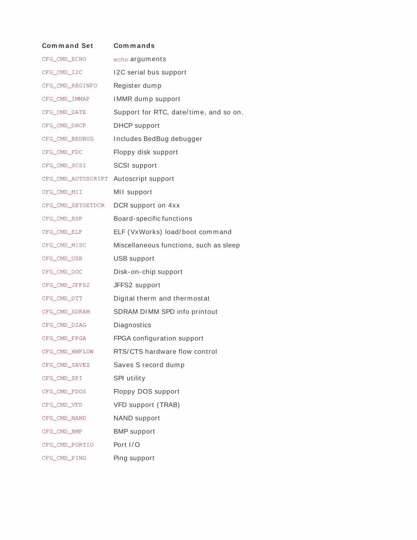
Command Set Commands
CFG_CMD_ECHO echo arguments
CFG_CMD_I2C I2C serial bus support
CFG_CMD_REGINFO Register dump
CFG_CMD_IMMAP IMMR dump support
CFG_CMD_DATE Support for RTC, date/time, and so on.
CFG_CMD_DHCP DHCP support
CFG_CMD_BEDBUG Includes BedBug debugger
CFG_CMD_FDC Floppy disk support
CFG_CMD_SCSI SCSI support
CFG_CMD_AUTOSCRIPT Autoscript support
CFG_CMD_MII MII support
CFG_CMD_SETGETDCR DCR support on 4xx
CFG_CMD_BSP Board-specific functions
CFG_CMD_ELF ELF (VxWorks) load/boot command
CFG_CMD_MISC Miscellaneous functions, such as sleep
CFG_CMD_USB USB support
CFG_CMD_DOC Disk-on-chip support
CFG_CMD_JFFS2 JFFS2 support
CFG_CMD_DTT Digital therm and thermostat
CFG_CMD_SDRAM SDRAM DIMM SPD info printout
CFG_CMD_DIAG Diagnostics
CFG_CMD_FPGA FPGA configuration support
CFG_CMD_HWFLOW RTS/CTS hardware flow control
CFG_CMD_SAVES Saves S record dump
CFG_CMD_SPI SPI utility
CFG_CMD_FDOS Floppy DOS support
CFG_CMD_VFD VFD support (TRAB)
CFG_CMD_NAND NAND support
CFG_CMD_BMP BMP support
CFG_CMD_PORTIO Port I/O
CFG_CMD_PING Ping support

Command Set Commands
CFG_CMD_MMC MMC support
CFG_CMD_FAT FAT support
CFG_CMD_IMLS Lists all found images
CFG_CMD_ITEST Integer (and string) test
CFG_CMD_NFS NFS support
CFG_CMD_REISER Reiserfs support
CFG_CMD_CDP Cisco Discovery Protocol
CFG_CMD_XIMG Loads part of multi-image
CFG_CMD_UNIVERSE Tundra Universe support
CFG_CMD_EXT2 EXT2 support
CFG_CMD_SNTP SNTP support
CFG_CMD_DISPLAY Display support

Appendix C. BusyBox CommandsBusyBox has many useful commands. Here is a list of the commands documented in a recentBusyBox snapshot.
[Pages 485 - 490]
addgroup Adds a group to the system
adduser Adds a user to the system
adjtimex Reads and optionally sets system timebase parameters
ar Extracts or lists files from an ar archive
arping Pings hosts by ARP requests/replies
ash The ash shell (command interpreter)
awk Pattern-scanning and -processing language
basename Strips directory path and suffixes from files
bunzip2 Uncompresses a file (or standard input if no input file specified)
bzcat Uncompresses to stdout
cal Displays a calendar
cat Concatenates file(s) and prints them to stdout
chgrp Changes the group membership of each file
chmod Changes file access permissions
chown Changes the owner and/or group of file(s)
chroot Runs the command with root directory set to new root
chvt Changes the foreground virtual terminal to /dev/ttyN
clear Clears screen
cmp Compares files
cp Copies files
cpio Extracts or lists files from a cpio archive
crond BusyBox's version of cron daemon

crontab Manages crontab control file
cut Prints selected fields from each input file to standard output
date Displays or sets the system time
dc Tiny RPN calculator
dd Copies a file, converting and formatting according to options
deallocvt Deallocates unused virtual terminal /dev/ttyN
delgroup Deletes a group from the system
deluser Deletes a user from the system
devfsd Obsolete daemon for managing devfs permissions and old device namesymlinks
df Prints the file system space used and space available
dirname Strips a nondirectory suffix from a filename
dmesg Prints or controls the kernel ring buffer
dos2unix Converts a file from DOS format to UNIX format
dpkg Utility to install, remove, and manage Debian packages
dpkg-deb Performs actions on Debian packages (debs)
du Summarizes disk space used for each file and/or directory
dumpkmap Prints a binary keyboard-translation table to standard output
dumpleases Displays the DHCP leases granted by udhcpd
echo Prints the specified ARGs to stdout
env Prints the current environment or runs a program after setting
expr Prints the value of an expression to standard output
false Returns an exit code of FALSE (1)
fbset Shows and modifies frame buffer settings
fdflush Forces floppy disk drive to detect disk change
fdformat Low-level-formats a floppy disk
fdisk Changes partition table
find Searches for files in a directory hierarchy
fold Wraps input lines in each file
free Displays the amount of free and used system memory
freeramdisk Frees all memory used by the specified ramdisk

fsckminix Performs a consistency check for MINIX file systems
ftpget Retrieves a remote file via FTP
ftpput Stores a local file on a remote machine via FTP
getopt Parses command options
getty Opens a tty, prompts for a login name, and then invokes /bin/login
grep Searches for PATTERN in each file or standard input
gunzip Uncompresses file (or standard input)
gzip Compresses file(s) with maximum compression
halt Halts the system
hdparm Gets/sets hard disk parameters
head Prints first 10 lines of each file to standard output
hexdump Dumps files in user-specified binary, octal, hex, character, or decimal format
hostid Prints a unique 32-bit identifier for the machine
hostname Gets or sets the hostname
httpd Listens for incoming http server requests
hwclock Queries and sets the hardware clock (RTC)
id Prints information for USERNAME or the current user
ifconfig Configures a network interface
ifdown Deconfigures an interface
ifup Configure an interface
inetd Listenss for network connections and launches programs
init BusyBox version of init
insmod Loads the specified kernel modules into the kernel
install Copies files and sets attributes
ip TCP/IP configuration utility
ipaddr Manipulates interface addresses
ipcalc Calculates IP network settings from an IP address
iplink Manipulates interface settings
iproute Displays/sets routing table entries
iptunnel BusyBox iptunnel utility
kill Sends a signal (default is SIGTERM) to the specified process(es)

killall Sends a signal (default is SIGTERM) to the specified process(es)
klogd Kernel logger
lash The BusyBox LAme SHell (command interpreter)
last Shows a listing of the last users who logged into the system
length Prints the length of the specified STRING
ln Creates a link named LINK_NAME or DIRECTORY to the specified TARGET
loadfont Loads a console font from standard input
loadkmap Loads a binary keyboard-translation table from standard input
logger Writes MESSAGE to the system log
login Begins a new session on the system
logname Prints the name of the current user
logread Shows the messages from syslogd
losetup Associates LOOPDEVICE with file
ls Lists directory contents
lsmod Lists the currently loaded kernel modules
makedevs Creates a range of block or character special files
md5sum Prints or checks MD5 checksums
mesg mesg controls write access to your terminal
mkdir Creates directory entries
mkfifo Creates a named pipe (identical to mknod name p)
mkfsminix Makes a MINIX file system
mknod Creates a special file (block, character, or pipe)
mkswap Prepares a disk partition to be used as a swap partition
mktemp Creates a temporary file with its name based on TEMPLATE
modprobe Used for high-level module loading and unloading
more Filter for viewing files one screenful at a time
mount Mounts a file system
mt Controls magnetic tape drive operation
mv Renames and/or moves files
nameif Renames a network interface while in the down state
nc Netcat opens a pipe to IP:port

netstat Netstat displays Linux networking information
nslookup Queries the nameserver for the IP address of the given host
od Dumps files in octal and other formats
openvt Starts a command on a new virtual terminal
passwd Changes a user password
patch BusyBox implementation of patch
pidof Gets PID of named process
ping Sends ICMP ECHO_REQUEST packets to network hosts
ping6 Sends ICMP ECHO_REQUEST packets to network hosts
pivot_root Changes the root file system
poweroff Halts the system and requests that the kernel shut off the power
printf Formats and prints arguments according to user format
ps Reports process status
pwd Prints the full filename of the current working directory
rdate Gets and possibly sets the system date and time from a remote HOST
readlink Displays the value of a symbolic link
realpath Returns the absolute pathnames of a given argument
reboot Reboots the system
renice Changes priority of running processes in allowed priorities range
reset Resets the screen
rm Removes (unlink) file(s)
rmdir Removes directory(ies), if they are empty
rmmod Unloads the specified kernel modules from the kernel
route Edits the kernel's routing tables
rpm Manipulates RPM packages
rpm2cpio Outputs a cpio archive of the rpm file
run-parts Runs a bunch of scripts in a directory
rx Receives a file using the xmodem protocol
sed Busybox Stream Editor implementation
seq Prints a range of numbers to standard output
setkeycodes Sets entries into the kernel's scancode-to-keycode map

sha1sum Prints or checks SHA1 checksums
sleep Delay for specified amount of time
sort Sorts lines of text in the specified files
start-stop-daemon Program to start and stop services
strings Displays printable strings in a binary file
stty Displays and modifies terminal settings
su Changes user ID or become root
sulogin Single user login
swapoff Disables virtual memory page swapping
swapon Enables virtual memory page swapping
sync Writes all buffered file system blocks to disk
sysctl Configures kernel parameters at runtime
syslogd Linux system and kernel-logging utility
tail Prints last 10 lines of each file to standard output
tar Creates, extracts, or lists files from a tar file
tee Copies standard input to each file and also to standard output
telnet BusyBox Telnet client implementation
telnetd BusyBox Telnet server implementation
test Checks file types and compares values, returning an exit
tftp Transfers a file using TFTP protocol
time Measures time used by a program
top Provides a view of processor activity in real time
touch Updates the last-modified date on the given FILE[s]
tr Translates, squeezes, and/or deletes characters
traceroute Traces the route IP packets follow
true Returns an exit code of trUE (0)
tty Prints the filename of the terminal connected to standard input
udhcpc BusyBox DHCP client implementation
udhcpd BusyBox DHCP server implementation
umount Unmount file systems
uname Prints certain system information

uncompress Uncompresses Z file(s)
uniq Discards all but one of successive identical lines from INPUT
unix2dos Converts file from UNIX format to DOS format
unzip Extracts files from ZIP archives
uptime Displays the time since the last boot
usleep Pauses for n microseconds
uudecode Uudecodes a file that is uuencoded
uuencode Uuencodes a file
vconfig Lets you create and remove virtual Ethernet devices
vi BusyBox vi editor
vlock Locks a virtual terminal and requires a password to unlock it
watch Executes a program periodically
watchdog Periodically writes to a specified watchdog device
wc Prints line, word, and byte counts for each file
wget Retrieves files via HTTP or FTP
which Locates a command on the current path
who Prints the current usernames and related information
whoami Prints the username associated with the current effective user ID
xargs Executes a command on every item given by standard input
yes Repeatedly outputs a line with all specified STRING(s), or y
zcat Uncompresses to stdout


Appendix D. SDRAM InterfaceConsiderationsIn this appendix
SDRAM Basics page 492
Clocking page 494
SDRAM Setup page 495
Summary page 500
At first glance, programming an SDRAM controller can seem like a formidable task. Indeed, numerousSynchronous Dynamic Random Access Memory (DRAM) technologies have been developed. In anever-ending quest for performance and density, many different architectures and modes ofoperation have been developed.
We examine the AMCC PowerPC 405GP processor for this discussion of SDRAM interfaceconsiderations. You might want to have a copy of the user manual to reference while we explore theissues related to SDRAM interfacing. This document is referenced in Section D.4.1, "Suggestions forAdditional Reading."

D.1. SDRAM Basics
To understand SDRAM setup, it is necessary to understand the basics of how an SDRAM deviceoperates. Without going into the details of the hardware design, an SDRAM device is organized as amatrix of cells, with a number of address bits dedicated to row addressing and a number dedicated tocolumn addressing. Figure D-1 illustrates this.
Figure D-1. Simplified SDRAM block diagram
Inside the memory matrix, the circuitry is quite complex. A simplified example of a read operation isas follows: A given memory location is referenced by placing a row address on the row address linesand then placing a column address on the column address lines. After some time has passed, thedata stored at the location addressed by the row and column inputs are made available to theprocessor on the data bus.
The processor outputs a row address on the SDRAM address bus and asserts its Row Address Select(RAS) signal. After a short preprogrammed delay to allow the SDRAM circuitry to capture the row

address, the processor outputs a column address and asserts its Column Address Select (CAS) signal.The SDRAM controller translates the actual physical memory address into row and column addresses.Many SDRAM controllers can be configured with the row and column width sizes; the PPC405GP isone of those examples. Later you will see that this must be configured as part of the SDRAMcontroller setup.
This example is much simplified, but the concepts are the same. A burst read, for example, whichreads four memory locations at once, outputs a single RAS and CAS cycle, and the internal SDRAMcircuitry automatically increments the column address for the subsequent three locations of the burstread, eliminating the need for the processor to issue four separate CAS cycles. This is but oneexample of performance optimization. The best way to understand this is to absorb the details of anactual memory chip. An example of a well-written data sheet is included in Section D.4.1,"Suggestions for Additional Reading."
D.1.1. SDRAM Refresh
An SDRAM is composed of a single transistor and a capacitor. The transistor supplies the charge, andthe capacitor's job is to retain (store) the value of the individual cell. For reasons beyond the scope ofthis discussion, the capacitor can hold the value for only a small duration. One of the fundamentalconcepts of dynamic memory is that the capacitors representing each cell must be periodicallyrecharged to maintain their value. This is referred to as SDRAM refresh.
A refresh cycle is a special memory cycle that neither reads nor writes data to the memory. It simplyperforms the required refresh cycle. One of the primary responsibilities of an SDRAM controller is toguarantee that refresh cycles are issued in time to meet the chip's requirements.
The chip manufacturers specify minimum refresh intervals, and it is the designer's job to guaranteeit. Usually the SDRAM controller can be configured directly to select the refresh interval. The PowerPC405GP presented here has a register specifically for this purpose. We will see this shortly.

D.2. Clocking
The term synchronous implies that the data read and write cycles of an SDRAM device coincide withthe clock signal from the CPU. SDR SDRAM is read and written on each SDRAM clock cycle. DDRSDRAM is read and written twice on each clock cycle, once on the rising edge of the clock and onceon the falling edge.
Modern processors have complex clocking subsystems. Many have multiple clock rates that are usedfor different parts of the system. A typical processor uses a relatively low-frequency crystal-generated clock source for its primary clock signal. A phase locked loop internal to the processorgenerates the CPU's primary clock (the clock rate we speak of when comparing processor speeds).Because the CPU typically runs much faster than the memory subsystem, the processor generates asubmultiple of the main CPU clock to feed to the SDRAM subsystem. You need to configure thisclocking ratio for your particular CPU and SDRAM combination.
The processor and memory subsystem clocks must be correctly configured for your SDRAM to workproperly. Your processor manual contains a section on clock setup and management, and you mustconsult this to properly set up your particular board design.
The AMCC 405GP is typical of processors of its feature set. It takes a single crystal-generated clockinput source and generates several internal and external clocks required of its subsystems. Itgenerates clocks for the CPU, PCI interface, Onboard Peripheral Bus (OPB), Processor Local Bus(PLB), Memory Clock (MemClk), and several internal clocks for peripherals such as timer and UARTblocks. A typical configuration might look like those in Table D-1.
Table D-1. Typical PPC405GP Clock Configuration
Clock Rate Comments
Crystal reference 33MHz Fundamental reference supplied to processor
CPU clock 133MHz Derived from processor's internal PLL, controlled byhardware pin strapping and register settings.
PLB clock 66MHz Derived from CPU clock and configured viahardware pin strapping and register settings. Usedfor internal processor local bus data interchangeamong its high-speed modules.
OPB clock 66MHz Derived from PLB clock and configured via registersettings. Used for internal connection of peripheralsthat do not need high-speed connection.
PCI clock 33MHz Derived from PLB clock and configured via registersettings.

Clock Rate Comments
MemClk 100MHz Drives the SDRAM chips directly. Derived from CPUclock and configured via register settings.
Decisions about clock setup normally must be made at hardware design time. Pin strapping optionsdetermine initial clock configurations upon application of power to the processor. Some control overderived clocks is often available by setting divider bits accessible through processor internal registersdedicated to clock and subsystem control. In the example we present here based on the 405GP, finalclock configuration is determined by pin strapping and firmware configuration. It is the bootloader'sresponsibility to set the initial dividers and any other clock options configurable via processor registerbits very early after power is applied.

D.3. SDRAM Setup
After the clocks have been configured, the next step is to configure the SDRAM controller. Controllersvary widely from processor to processor, but the end result is always the same: You must providethe correct clocking and timing values to enable and optimize the performance of the SDRAMsubsystem.
As with other material in this book, there is no substitute for detailed knowledge of the hardware youare trying to configure. This is especially so for SDRAM. It is beyond the scope of this appendix toexplore the design of SDRAM, but some basics must be understood. Many manufacturers' data sheetson SDRAM devices contain helpful technical descriptions. You are urged to familiarize yourself withthe content of these data sheets. You don't need a degree in hardware engineering to understandwhat must be done to properly configure your SDRAM subsystem, but you need to invest in somelevel of understanding.
Here we examine how the SDRAM controller is configured on the 405GP processor as configured bythe U-Boot bootloader we covered in Chapter 7 , "Bootloaders." Recall from Chapter 7 that U-Bootprovides a hook for SDRAM initialization from the assembly language startup code found in start.S inthe 4xx-specific cpu directory. Refer back to Section 7.4.4 "Board-Specific Initialization" in Chapter 7 .Listing D-1 reproduces the sdram_init() function from U-Boot's .../cpu/ppc4xx/sdram.c file.
Listing D. ppc4xx sdram_init() from U-Boot
01 void sdram_init(void)02{03 ulong sdtr1;04 ulong rtr;05 int i;06
07 /*08 * Support for 100MHz and 133MHz SDRAM09 */10 if (get_bus_freq(0) > 100000000) {11 /*12

* 133 MHz SDRAM13 */14 sdtr1 = 0x01074015;15 rtr = 0x07f00000;16 } else {17 /*18 * default: 100 MHz SDRAM19 */20 sdtr1 = 0x0086400d;21 rtr = 0x05f00000;22 }23
24 for (i=0; i<N_MB0CF; i++) {25 /*26 * Disable memory controller.27 */28 mtsdram0(mem_mcopt1, 0x00000000);29
30 /*31 * Set MB0CF for bank 0.32 */33 mtsdram0(mem_mb0cf, mb0cf[i].reg);34 mtsdram0(mem_sdtr1, sdtr1);35 mtsdram0(mem_rtr, rtr);36
37 udelay(200);38

39 /*40 * Set memory controller options reg, MCOPT1.41 * Set DC_EN to '1' and BRD_PRF to '01' for 16 byte PLB Burst42 * read/prefetch.43 */44 mtsdram0(mem_mcopt1, 0x80800000);45
46 udelay(10000);47
48 if (get_ram_size(0, mb0cf[i].size) == mb0cf[i].size) {49 /*50 * OK, size detected -> all done51 */52 return;53 }54 }55}
The first action reads the pin strapping on the 405GP processor to determine the design value for theSDRAM clock. In this case, we can see that two possible values are accommodated: 100MHz and133MHz. Based on this choice, constants are chosen that will be used later in the function to set theappropriate register bits in the SDRAM controller.
Starting on line 24, a loop is used to set the parameters for each of up to five predefined memorysizes. Currently, U-Boot has logic to support a single bank of memory sized at 4MB, 16MB, 32MB,64MB, or 128MB. These sizes are defined in a table called mb0cf in .../cpu/ppc4xx/sdram.c . Thetable associates a constant with each of these memory sizes, based on the value required in the405GP memory bank configuration register. The loop does this:
for (i = each possible memory bank size, largest first) { select timing constant based on SDRAM clock speed; disable SDRAM memory controller; configure bank 0 with size[i], timing constants[i] re-enable SDRAM memory controller;

run simple memory test to dynamically determine size; /* This is done using get_ram_size() */ if ( tested size == configured size ) done;}
This simple logic simply plugs in the correct timing constants in the SDRAM controller based onSDRAM clock speed and configured memory bank size from the hard-coded table in U-Boot. Usingthis explanation, you can easily correlate the bank configuration values using the 405GP referencemanual. For a 64MB DRAM size, the memory bank control register is set as follows:
Memory Bank 0 Control Register = 0x000a4001
The PowerPC 405GP User's Manual describes the fields in Table D-2 for the memory bank 0 controlregister.
Bank Address (BA)
0x00
Starting memory address of this bank.
Size (SZ)
0x4
Size of this memory bankin this case, 64MB.
Addressing Mode (AM)
0x2
Determines the organization of memory, including the number of row and column bits. In this case,Mode 2 = 12 row address bits, and either 9 or 10 column address bits, and up to four internal SDRAMbanks. This data is provided in a table in the 405GP user's manual.
Bank Enable (BE)
0x1
Enable bit for the bank configured by this register. There are four of these memory bankconfiguration registers in the 405GP.
Table D-2. 405GP Memory Bank 0-3 Configuration RegisterFields
Field Value Comments

The values in this table must be determined by the designer, based on the choice of memory modulein use on the board.
Let's look at a timing example for more detail on the timing requirements of a typical SDRAMcontroller. Assuming a 100MHz SDRAM clock speed and 64MB memory size, the timing constantsselected by the sdram_init() function in Listing D-1 are selected as follows:
SDRAM Timing Register = 0x0086400dRefresh Timing Register = 0x05f00000
The PowerPC 405GP User's Manual describes the fields in Table D-3 for the SDRAM Timing Register.
CAS Latency (CASL)
0x1
SDRAM CAS Latency. This value comes directly from the SDRAM chip specifications. It is the delay inclock cycles required by the chip between issuance of the read command (CAS signal) until the datais available on the data bus. In this case, the 0x1 represents two clock cycles, as seen from the405GP user's manual.
Precharge Command to Next Activate (PTA)
0x1
The SDRAM Precharge command deactivates a given row. In contrast, the Activate commandenables a given row for subsequent access, such as during a burst cycle. This timing parameterenforces the minimum time between Precharge to a subsequent Activate cycle and is dictated by theSDRAM chip. The correct value must be obtained from the SDRAM chip specification. In this case, 0x1represents two clock cycles, as determined from the 405GP user's manual.
Read/Write to Precharge Command Minimum (CTP)
0x2
This timing parameter enforces the minimum time delay between a given SDRAM read or writecommand to a subsequent Precharge command. The correct value must be obtained from the SDRAMchip specification. In this case, 0x2 represents three clock cycles, as determined from the 405GPuser's manual.
SDRAM Command Leadoff (LDF)
0x1
This timing parameter enforces the minimum time delay between assertion of address or commandcycle to bank select cycle. The correct value must be obtained from the SDRAM chip specification. Inthis case, 0x1 represents two clock cycles, as determined from the 405GP user's manual.
Table D-3. 405GP SDRAM Timing Register Fields

Field Value Comments
The final timing parameter configured by the U-Boot example in Listing D-1 is the refresh timingregister value. This register requires a single field that determines the refresh interval enforced bythe SDRAM controller. The field representing the interval is treated as a simple counter running at theSDRAM clock frequency. In the example here, we assumed 100MHz as the SDRAM clock frequency.The value programmed into this register in our example is 0x05f0_0000. From the PowerPC 405GPUser's Manual, we determine that this will produce a refresh request every 15.2 microseconds. Aswith the other timing parameters, this value is dictated by the SDRAM chip specifications.
A typical SDRAM chip requires one refresh cycle for each row. Each row must be refreshed in theminimum time specified by the manufacturer. In the chip referenced in Section D.4.1 , "Suggestionsfor Additional Reading," the manufacturer specifies that 8,192 rows must be refreshed every 64milliseconds. This requires generating a refresh cycle every 7.8 microseconds to meet thespecifications for this particular device.

D.4. Summary
SDRAM devices are quite complex. This appendix presented a very simple example to help younavigate the complexities of SDRAM controller setup. The SDRAM controllers perform a criticalfunction and must be properly set up. There is no substitute to diving into a specification anddigesting the information presented. The two example documents referenced in this appendix areexcellent starting points.
D.4.1. Suggestions for Additional Reading
AMCC 405GP Embedded Processor User's ManualAMCC Corporationwww.amcc.com/Embedded/
Micron Technology, Inc.Synchronous DRAM MT48LC64M4A2 Data Sheethttp://download.micron.com/pdf/datasheets/dram/sdram/256MSDRAM.pdf

Appendix E. Open Source ResourcesSource Repositories and Developer Information
Mailing Lists
Linux News and Developments
Open Source Insight and Discussion

Source Repositories and Developer Information
Several locations on the Web focus on Linux development. Here is a list of the most importantwebsites for the various architectures and projects:
Primary kernel source tree
www.kernel.org
Primary kernel GIT repository
www.kernel.org/git
PowerPC-related development and mailing lists
http://ozlabs.org/
MIPS-related developments
www.linux-mips.org
ARM-related Linux development
www.arm.linux.org.uk
Primary home for a huge collection of open-source projects
http://sourceforge.net

Mailing Lists
Hundreds, if not thousands, of mailing lists cater to every aspect of Linux and open-sourcedevelopment. Here are a few to consider. Make sure you familiarize yourself with mailing listetiquette before posting to these lists.
Most of these lists maintain archives that are searchable. This is the first place that you shouldconsult. In a great majority of the cases, your question has already been asked and answered. Startyour reading here, for advice on how to best use the public mail lists:
The Linux Kernel Mailing List FAQ
www.tux.org/lkml
List server serving various Linux kernel-related mail lists
http://vger.kernel.org
Linux Kernel Mailingvery high volume, kernel development only
http://vger.kernel.org/vger-lists.html#linux-kernel

Linux News and Developments
Many news sites are worth browsing occasionally. Some of the more popular are listed here.
LinuxDevices.com
www.linuxdevices.com
PowerPC News and other information
http://penguinppc.org
General Linux News and Developments
www.lwn.net

Open Source Insight and Discussion
The following public website contains useful information and education focusing on legal issuesaround open source.
www.open-bar.org

Appendix F. Sample BDI-2000Configuration File
; bdiGDB configuration file for the UEI PPC 5200 Board; Revision 1.0; Revision 1.1 (Added serial port setup); -----------------------------------------------------------; 4 MB Flash (Am29DL323); 128 MB Micron DDR DRAM;[INIT]; init core registerWREG MSR 0x00003002 ;MSR : FP,ME,RIWM32 0x80000000 0x00008000 ;MBAR : internal registers at 0x80000000 ; Default after RESET, MBAR sits at 0x80000000 ; because it's POR value is 0x0000_8000 (!)
WSPR 311 0x80000000 ; MBAR : save internal register offset ; SPR311 is the MBAR in G2_LE
WSPR 279 0x80000000 ;SPRG7: save internal memory offsetReg: 279
; Init CDM (Clock Distribution Module); Hardware Reset config {; ppc_pll_cfg[0..4] = 01000b: XLB:Core -> 1:3: Core:f(VCO) -> 1:2: XLB:f(VCO) -> 1:6;; xlb_clk_sel = 0 -> XLB_CLK=f(sys) / 4 = 132 MHz;; sys_pll_cfg_1 = 0 -> NOP; sys_pll_cfg_0 = 0 -> f(sys) = 16x SYS_XTAL_IN = 528 MHz; };; CDM Configuration RegisterWM32 0x8000020c 0x01000101 ; enable DDR Mode ; ipb_clk_sel = 1 -> XLB_CLK / 2 (ipb_clk = 66 MHz) ; pci_clk_sel = 01 -> IPB_CLK/2
; CS0 FlashWM32 0x80000004 0x0000ff00 ;CS0 start = 0xff000000 - Flash memory is on

CS0WM32 0x80000008 0x0000ffff ;CS0 stop = 0xffffffff
; IPBI Register and Wait State EnableWM32 0x80000054 0x00050001 ;CSE: enable CS0, disable CSBOOT, ;Wait state enable\ ; CS2 also enabled
WM32 0x80000300 0x00045d30 ;BOOT ctrl ; bits 0-7: WaitP (try 0xff) ; bits 8-15: WaitX (try 0xff) ; bit 16: Multiplex or non-mux'ed (0x0 = non-muxed) ; bit 17: reserved (Reset value = 0x1, keep it) ; bit 18: Ack Active (0x0) ; bit 19: CE (Enable) 0x1 ; bits 20-21: Address Size (0x11 = 25/6 bits) ; bits 22:23: Data size field (0x01 = 16-bits) ; bits 24:25: Bank bits (0x00) ; bits 26-27: WaitType (0x11) ; bits 28: Write Swap (0x0 = no swap) ; bits 29: Read Swap (0x0 = no swap) ; bit 30: Write Only (0x0 = read enable) ; bit 31: Read Only (0x0 = write enable)
; CS2 Logic RegistersWM32 0x80000014 0x0000e00eWM32 0x80000018 0x0000efff
; LEDS:; LED1 - bits 0-7; LED2 - bits 8-15; LED3 - bits 16-23; LED4 - bits 24-31; off = 0x01; on = 0x02; mm 0xe00e2030 0x02020202 1 (all on); mm 0xe00e2030 0x01020102 1 (2 on, 2 off)
WM32 0x80000308 0x00045b30 ; CS2 Configuration Register ; bits 0-7: WaitP (try 0xff) ; bits 8-15: WaitX (try 0xff) ; bit 16: Multiplex or non-mux'ed (0x0 =non-muxed) ; bit 17: reserved (Reset value = 0x1, keep it) ; bit 18: Ack Active (0x0) ; bit 19: CE (Enable) 0x1 ; bits 20-21: Address Size (0x10 = 24 bits) ; bits 22:23: Data size field (0x11 = 32-bits) ; bits 24:25: Bank bits (0x00) ; bits 26-27: WaitType (0x11) ; bits 28: Write Swap (0x0 = no swap) ; bits 29: Read Swap (0x0 = no swap)

; bit 30: Write Only (0x0 = read enable) ; bit 31: Read Only (0x0 = write enable)
WM32 0x80000318 0x01000000 ; Master LPC Enable
;; init SDRAM controller;; For the UEI PPC 5200 Board,; Micron 46V32M16-75E (8 MEG x 16 x 4 banks); 64 MB per Chip, for a total of 128 MB; arranged as a single "space" (i.e 1 CS); with the following configuration:; 8 Mb x 16 x 4 banks; Refresh count 8K; Row addressing: 8K (A0..12) 13 bits; Column addressing: 1K (A0..9) 10 bits; Bank Addressing: 4 (BA0..1) 2 bits; Key Timing Parameters: (-75E); Clockrate (CL=2) 133 MHz; DO Window 2.5 ns; Access Window: +/- 75 ns; DQS - DQ Skew: +0.5 ns; t(REFI): 7.8 us MAX;; Initialization Requirements (General Notes); The memory Mode/Extended Mode registers must be; initialized during the system boot sequence. But before; writing to the controller Mode register, the mode_en and; cke bits in the Control register must be set to 1. After; memory initialization is complete, the Control register; mode_en bit should be cleared to prevent subsequent access; to the controller Mode register.
; SDRAM init sequence; 1) Setup and enable chip selects; 2) Setup config registers; 3) Setup TAP Delay
; Setup and enable SDRAM CSWM32 0x80000034 0x0000001a ;SDRAM CS0, 128MB @ 0x00000000WM32 0x80000038 0x08000000 ;SDRAM CS1, disabled @ 0x08000000
WM32 0x80000108 0x73722930 ;SDRAM Config 1 Samsung ; Assume CL=2 ; bits 0-3: srd2rwp: in clocks (0x6) ; bits 507: swt2rwp: in clocks -> Data sheet suggests ; 0x3 for DDR (0x3) ; bits 8-11: rd_latency -> for DDR 0x7 ; bits 13-15: act2rw -> 0x2 ; bit 16: reserved ; bits 17-19: pre2act -> 0x02

; bits 20-23: ref2act -> 0x09 ; bits 25-27: wr_latency -> for DDR 0x03 ; bits 28-31: Reserved
WM32 0x8000010c 0x46770000 ;SDRAM Config 2 Samsung ; bits 0-3: brd2rp -> for DDR 0x4 ; bits 4-7: bwt2rwp -> for DDR 0x6 ; bits 8-11: brd2wt -> 0x6 ; bits 12-15: burst_length -> 0x07 (bl - 1) ; bits 16-13: Reserved; Setup initial Tap delayWM32 0x80000204 0x18000000 ; Start in the end of the range (24 = 0x18)Samsung
WM32 0x80000104 0xf10f0f00 ;SDRAM Control (was 0xd14f0000) ; bit 0: mode_en (1=write) ; bit 1: cke (MEM_CLK_EN) ; bit 2: ddr (DDR mode on) ; bit 3: ref_en (Refresh enable) ; bits 4-6: Reserved ; bit 7: hi_addr (XLA[4:7] as row/col ; must be set to '1' 'cuz we need 13 RA bits ; for the Micron chip above ; bit 8: reserved ; bit 9: drive_rule - 0x0 ; bit 10-15: ref_interval, see UM 0x0f ; bits 16-19: reserved ; bits 20-23: dgs_oe[3:0] (not sure) ; but I think this is req'd for DDR 0xf ; bits 24-28: Resv'd ; bit 29: 1 = soft refresh ; bit 30 1 = soft_precharge ; bit 31: reserved
WM32 0x80000104 0xf10f0f02 ;SDRAM Control: precharge allWM32 0x80000104 0xf10f0f04 ;SDRAM Control: refreshWM32 0x80000104 0xf10f0f04 ;SDRAM Control: refresh
WM32 0x80000100 0x018d0000 ; SDRAM Mode Samsung ; bits 0-1: MEM_MBA - selects std or extended MODE reg 0x0 ; bits 2-13: MEM_MA (see DDR DRAM Data sheet) ; bits 2-7: Operating Mode -> 0x0 = normal ; bits 8-10: CAS Latency (CL) -> Set to CL=2 forDDR (0x2) ; bit 11: Burst Type: Sequential for PMC5200 ->0x0 ; bits 12-14: Set to 8 for MPC5200 -> 0x3 ; bit 15: cmd = 1 for MODE REG WRITE
WM32 0x80000104 0x710f0f00 ;SDRAM Control: Lock Mode Register (was0x514f0000)
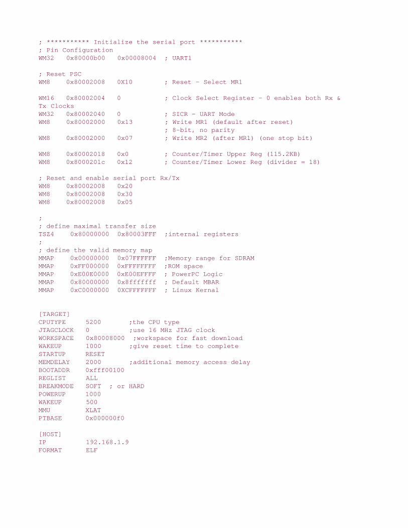
; *********** Initialize the serial port ***********; Pin ConfigurationWM32 0x80000b00 0x00008004 ; UART1
; Reset PSCWM8 0x80002008 0X10 ; Reset - Select MR1
WM16 0x80002004 0 ; Clock Select Register - 0 enables both Rx &Tx ClocksWM32 0x80002040 0 ; SICR - UART ModeWM8 0x80002000 0x13 ; Write MR1 (default after reset) ; 8-bit, no parityWM8 0x80002000 0x07 ; Write MR2 (after MR1) (one stop bit)
WM8 0x80002018 0x0 ; Counter/Timer Upper Reg (115.2KB)WM8 0x8000201c 0x12 ; Counter/Timer Lower Reg (divider = 18)
; Reset and enable serial port Rx/TxWM8 0x80002008 0x20WM8 0x80002008 0x30WM8 0x80002008 0x05
;; define maximal transfer sizeTSZ4 0x80000000 0x80003FFF ;internal registers;; define the valid memory mapMMAP 0x00000000 0x07FFFFFF ;Memory range for SDRAMMMAP 0xFF000000 0xFFFFFFFF ;ROM spaceMMAP 0xE00E0000 0xE00EFFFF ; PowerPC LogicMMAP 0x80000000 0x8fffffff ; Default MBARMMAP 0xC0000000 0XCFFFFFFF ; Linux Kernal
[TARGET]CPUTYPE 5200 ;the CPU typeJTAGCLOCK 0 ;use 16 MHz JTAG clockWORKSPACE 0x80008000 ;workspace for fast downloadWAKEUP 1000 ;give reset time to completeSTARTUP RESETMEMDELAY 2000 ;additional memory access delayBOOTADDR 0xfff00100REGLIST ALLBREAKMODE SOFT ; or HARDPOWERUP 1000WAKEUP 500MMU XLATPTBASE 0x000000f0
[HOST]IP 192.168.1.9FORMAT ELF

LOAD MANUAL ;load code MANUAL or AUTO after resetPROMPT uei>
[FLASH]CHIPTYPE AM29BX16 ;Flash type (AM29F | AM29BX8 | AM29BX16 | I28BX8 |I28BX16)CHIPSIZE 0x00400000 ;The size of one flash chip in bytesBUSWIDTH 16 ;The width of the flash memory bus in bits (8 | 16 |32)WORKSPACE 0x80008000 ;workspace in internal SRAMFILE u-boot.binFORMAT BIN 0xFFF00000ERASE 0xFFF00000 ;erase a sector of flashERASE 0xFFF10000 ;erase a sector of flashERASE 0xFFF20000 ;erase a sector of flashERASE 0xFFF30000 ;erase a sector of flashERASE 0xFFF40000 ;erase a sector of flash
[REGS]FILE $reg5200.def

Index
[SYMBOL] [A] [B] [C] [D] [E] [F] [G] [H] [I] [J] [K] [L] [M] [N] [O] [P] [Q] [R] [S] [T] [U] [V] [W] [X] [Z]

Index
[SYMBOL] [A] [B] [C] [D] [E] [F] [G] [H] [I] [J] [K] [L] [M] [N] [O] [P] [Q] [R] [S] [T] [U] [V] [W] [X] [Z]
+ (plus sign)
. (period)
/ (forward slash)
$T packet
32-bit
64-bit
855GM chipset

Index
[SYMBOL] [A] [B] [C] [D] [E] [F] [G] [H] [I] [J] [K] [L] [M] [N] [O] [P] [Q] [R] [S] [T] [U] [V] [W] [X] [Z]
access rights
add-symbol-file command
addr2line
address breakpoints
address space
Advanced Telecommunications Computing Architecture (ATCA) platform
Alchemy processors
AltiVec hardware
AMCC PowerPC processors
AMD MIPS processors
apache package
applets
applications
debugging
attaching to running processes
via serial ports
Flash resident code, debugging
with multiple processes, debugging
multithreaded applications, debugging
with shared libraries, debugging
target applications
debugging
debugging with gdbserver
stripping
/arch subdirectory, porting Linux 2nd
architecture branches, porting Linux
architecture objects, composite kernel image
architectures
hardware architecture example (embedded systems)
initialization flow of control
Linux-supported architectures
ARM processors 2nd
Freescale ARM processors
Intel ARM XScale processors
TI ARM processors
@ (at sign)
at sign (@)
ATCA platform

Index
[SYMBOL] [A] [B] [C] [D] [E] [F] [G] [H] [I] [J] [K] [L] [M] [N] [O] [P] [Q] [R] [S] [T] [U] [V] [W] [X] [Z]
backtrace command
BDI-2000 sample configuration file [See also JTAG probes.]
bd_info structure
Big Kernel Lock (BKL)
bin directory
binary utilities
addr2line
ldd
nm
objcopy
objdump
prelink
readelf
strings
strip
binutils
BIOS, bootloaders versus
bi_record structure
BKL (Big Kernel Lock)
block devices
block sizes
board-specific information, porting Linux
board-specific initialization
MTD
U-Boot porting example
boards [See hardware platforms; CPUs, porting U-Boot.]
boot block Flash chips
boot messages
booting [See also build system (kernel); initialization.]
debugging boot process
dumping printk log buffer
serial debug output
trapping crashes with KGDB
from disk with U-Boot
initrd
with KGDB enabled
bootloaders
BIOS versus
booting kernel
bootstrap loaders versus
DRAM controller setup

execution context
GRUB 2nd
image compiling and linking
initialization flow of control
architecture setup
head.o module
main.c module
initrd and
Lilo
memory addresses
nonvolatile storage versus RAM
porting Linux prerequisites
role of
selecting
starting target board
U-Boot
booting from disk
booting with KGDB enabled
command sets
configurable commands
configuration
debugging with JTAG probe
image format
initrd support
kernel, booting
network protocols
NFS root mount example
nonvolatile storage
porting
target board, starting
bootm command
BOOTP (Bootstrap Protocol), U-Boot network operations
BOOTP server, hosting target boards
bootstrap loaders
bottom-half processing
breakpoints
hardware versus software breakpoints
with KGDB
remote debugging
types of
Broadcom MIPS processors
browsing sysfs file system
build numbers
build output (kernel)
build system (kernel)
composite kernel image
architecture objects
boot messages
bootstrap loaders
Image object
configuration editors
dot-config file

Kconfig files
makefile targets
makefiles
building
device drivers
file systems
cramfs
JFFS2
initrd image
MTD (Memory Technology Devices) services
root file system
BusyBox
commands 2nd
configuring
cross-compiling
defined
example rcS initialization script
executables
init
operations
root file system
target installation
busybox package
bzImage target

Index
[SYMBOL] [A] [B] [C] [D] [E] [F] [G] [H] [I] [J] [K] [L] [M] [N] [O] [P] [Q] [R] [S] [T] [U] [V] [W] [X] [Z]
carrier grade Linux, standards for
cbrowser
CFI (Common Flash Interface) drivers
character devices
child processes, debugging
chipsets
clocking SDRAM
command line, kernel command line
command sets, U-Boot
command-line partitioning (MTD)
commands
backtrace
BusyBox 2nd
configurable commands, U-Boot
continue
fis list
gdb frame
gdb print
mkfs.jffs2
user-defined commands
.gdbinit file
list of
module_init( )
commercial embedded Linux distributions
Common Flash Interface (CFI) drivers
CompactFlash modules
CompactPCI platform
compilers, cross-development environment
compiling
bootloader images
kernel
optimization during
composite kernel image
architecture objects
boot messages
bootstrap loaders
Image object
.config file [See also configuration files; configuration.]
MTD (Memory Technology Devices) configuration
configurable commands, U-Boot
configuration

BusyBox
KGDB
of kernel, Kconfig files
MTD (Memory Technology Devices) services
MTD (Memory Technology Devices) subsystem
U-Boot
configuration editors
configuration files
BDI-2000 sample configuration file
JTAG probes
configuration rules, U-Boot porting example
CONFIG_MTD_CHAR element (MTD configuration)
CONFIG_SERIAL_TEXT_DEBUG
connections
to KGDB
JTAG probes
contexts [See execution contexts.]
continue command
remote debugging
controllers (SDRAM), setup
controllers boards [See hardware platforms.]
converting
ext2 file system to ext3 file system
spinlocks to mutexes
core dumps, debugging
Coyote, board-specific MTD initialization
coyote_init( ) function
cPCI platform
cpuinfo entry (/proc file system)
CPUs, porting U-Boot [See CPUs, porting U-Boot.]
cramfs file system
creating
directory structure
crashes, trapping with KGDB
critical sections
management in real-time kernel patch
preventing kernel preemption
cross-compiling BusyBox
cross-debugging [See remote debugging.]
cross-development environment 2nd
hello world (embedded)
cscope
custom configuration options
customizing
kernel initialization
platform-specific code
cylinders

Index
[SYMBOL] [A] [B] [C] [D] [E] [F] [G] [H] [I] [J] [K] [L] [M] [N] [O] [P] [Q] [R] [S] [T] [U] [V] [W] [X] [Z]
Das U-Boot [See U-Boot.]
data breakpoints
dd utility
DDD (Data Display Debugger)
deadlock conditions, debugging
debug sessions
DDD
GDB
debug statements in initcalls
debugging
applications
attaching to running processes
Flash resident code
with multiple processes
with multiple threads
remote debugging
via serial ports
with shared libraries
target applications
core dumps
hardware-assisted debugging
kernel
challenges of
customizing platform-specific code
dumping the printk log buffer
.gdbinit file
with JTAG probes
with KGDB 2nd
loadable modules, debugging
macros, list of
with Magic SysReq key
optimization and
with printk function
remote debugging
serial debug output
real-time kernel
deadlock conditions
interrupt off history
interrupt off timing
latency tracing
preemption debugging

runtime control of locking mode
soft lockup detection
wakeup latency history
wakeup timing
default kernel command line
deleting .config file
Denk, Wolfgang
dependencies
depmod utility
resolving
depmod utility
derived works
detach command
detecting Redboot partitions
dev directory
development setup example (embedded Linux)
device drivers [See also loadable modules.]
block devices
build infrastructure
character devices
device nodes
exercising
GPL and
installing
loading and unloading
major numbers
methods
minimal device driver example
minor numbers
purpose of
utilities
depmod
insmod
lsmod
mknod
modinfo
modprobe
parameters for
rmmod
device nodes
DHCP (Dynamic Host Control Protocol), U-Boot network operations
DHCP server, hosting target boards
directories
installing device drivers
subdirectories in kernel
top-level source directory
disk subsystem, booting from with U-Boot
distribution engineering
distributions
dmalloc 2nd
do-it-yourself embedded Linux distributions
documentation of kernel

dot-config file [See also configuration files; configuration.]
MTD (Memory Technology Devices) configuration
DRAM controllers, setup
drivers [See also device drivers.]
CFI (Common Flash Interface) drivers
MTD Flash chip drivers
MTD mapping drivers
Dynamic Host Control Protocol (DHCP), U-Boot network operations
Dynamic Random Access Memory (DRAM) controllers, setup
dynamically loadable modules

Index
[SYMBOL] [A] [B] [C] [D] [E] [F] [G] [H] [I] [J] [K] [L] [M] [N] [O] [P] [Q] [R] [S] [T] [U] [V] [W] [X] [Z]
e2fsck utility
clean file system check
corrupted file system check
e600 core
early serial debug output
early variable access
ELDK (Embedded Linux Development Kit)
embedded Linux [See also embedded systems; Linux.]
advantages of
components needed
development setup example
distributions
usage statistics
Embedded Linux Development Kit (ELDK)
embedded systems
BIOS versus bootloaders
characteristics of
cross-development environment
hardware architecture example
kernel
booting
initializing
user space processes
processors [See processors.]
storage in
address space
execution contexts
Flash file systems
Flash memory
NAND Flash memory
process virtual memory
target board, starting
enabling
KGDB
MTD (Memory Technology Devices) services
remote debugging
environments, cross-development environments
EP405 board (U-Boot porting example)
board-specific initialization
makefile configuration rule
processor initialization

erase blocks (Flash memory)
/etc/exports file
etc directory
/etc/exports file
events, shared library events in GDB
executables, BusyBox
execution contexts
bootloaders
execve( ) function
exercising device drivers
exports file (/etc directory)
ext2 file system (Second Extended File System)
checking integrity of
clean file system check
corrupted file system check
converting to ext3
inodes
mounting
mounting MTD Flash partitions as
partitions, formatting 2nd
ext3 file system (Third Extended File System)
converting ext2 file systems to
definition of
journal files

Index
[SYMBOL] [A] [B] [C] [D] [E] [F] [G] [H] [I] [J] [K] [L] [M] [N] [O] [P] [Q] [R] [S] [T] [U] [V] [W] [X] [Z]
fdisk utility
FHS (File System Hierarchy Standard)
file system operation methods for device drivers
file systems
building
cramfs
creating
directory structure
ext2 (Second Extended File System)
checking integrity of
converting to ext3
mounting
mounting MTD Flash partitions as
partition formatting
ext3 (Third Extended File System)
converting ext2 file systems to
definition of
journal files
Flash file systems
hard disk partitions
block sizes
definition of
displaying information about
formatting
types of
inodes
JFFS2 (Journaling Flash File System)
building
creating on MTD subsystem
directory structure
mounting on MTD subsystem
journaling file systems
NFS (Network File System)
/etc/exports file
kernel configuration
mounting
root file system
/proc
cpuinfo entry
init process
maps entry

mount dependency
mounting
ramfs
ReiserFS
root file system
building
defined
distribution engineering
FHS (File System Hierarchy Standard)
minimal file system
mounting 2nd
top-level directories
sysfs
browsing
top-level directory
tmpfs
files
dot-config file
MTD (Memory Technology Devices) configuration
ext3 journal files
hidden files
listing
find_next_task macro
find_task macro
fis list command
Flash chip drivers (MTD)
Flash file systems
Flash Image System commands
Flash memory
NAND Flash
usage
Flash programming with JTAG probes
Flash resident code, debugging
flashcp utility (MTD)
flash_* utilities (MTD)
flash_erase utility (MTD)
flow of control (initialization)
architecture setup
head.o module
main.c module
fork( ) system call, debugging multiple processes
formatting partitions
forward slash (/)
free, freedom versus
freedom, free versus
Freescale ARM processors
Freescale MPC7448 processors
Freescale PowerPC processors
functions
coyote_init( )
init_pq2fads_mtd( )
inline functions

kernel debugging and
physmap_configure( )

Index
[SYMBOL] [A] [B] [C] [D] [E] [F] [G] [H] [I] [J] [K] [L] [M] [N] [O] [P] [Q] [R] [S] [T] [U] [V] [W] [X] [Z]
G4 core, Freescale MPC7448 processors
GCC, optimization
GDB (GNU Debugger) [See also debugging.]
core dumps
as cross-debugger
debug sessions
interfacing with JTAG probes
invoking
KGDB (Kernel GDB)
booting with KGDB enabled
breakpoints
kernel configuration
trapping crashes
shared library events in
gdb frame command
gdb print command
.gdbinit file
gdbserver
attaching to running processes
General Public License [See GPL (General Public License).]
glibc package
GNU Debugger [See GDB (GNU Debugger).]
GNU public license (GPL)
GPL (General Public License)
device drivers and
GPL (GNU public license)
GRUB (GRand Unified Bootloader)

Index
[SYMBOL] [A] [B] [C] [D] [E] [F] [G] [H] [I] [J] [K] [L] [M] [N] [O] [P] [Q] [R] [S] [T] [U] [V] [W] [X] [Z]
hard disks
cylinders
partitions
block sizes
definition of
displaying information about
formatting
types of
hard real time
hardware architecture example (embedded systems)
hardware breakpoints
software breakpoints versus
hardware platforms
ATCA
board-specific initialization
MTD
U-Boot porting example
CompactPCI
porting Linux to
board-specific information
customizing kernel initialization
default kernel command line
early variable access
final steps
machine-dependent calls
platform initialization
prerequisites
hardware-assisted debugging
hardware-debug probes, kernel debugging with
gdb interfaces with JTAG probes
programming Flash
head.o module, initialization flow of control
hello world (embedded), cross-development environments
Hennessey, John
hidden files
host system requirements
hosting target boards
BOOTP server
DHCP server
NFS server
target NFS root mount

TFTP server
U-Boot NFS root mount

Index
[SYMBOL] [A] [B] [C] [D] [E] [F] [G] [H] [I] [J] [K] [L] [M] [N] [O] [P] [Q] [R] [S] [T] [U] [V] [W] [X] [Z]
IBM 970FX processors
image (kernel) [See vmlinux (kernel proper).]
image format for U-Boot
Image object, composite kernel image
images, bootloader images, compiling and linking
include files, cross-development environment
incremental linking
__init macros
init process
BusyBox
in kernel boot process
inittab
/proc file system
runlevels
startup script example
user space processes
init thread
final boot steps
initcalls and
__initcall macros
initcalls, initialization via
initial RAM disk [See initrd.]
initialization
board-specific initialization, U-Boot porting example
init thread
final boot steps
initcalls and
kernel initialization [See kernel.]
platform initialization, porting Linux
processor initialization, U-Boot porting example
subsystem initialization
system initialization [See system initialization.]
with JTAG probes
initialization code, debugging loadable modules
initialization files, gdb
initialization flow of control
architecture setup
head.o module
main.c module
initramfs
initrd

booting
building image of
initramfs versus
linuxrc file and
mounting root file system
initscripts package
inittab system configuration file
init_pq2fads_mtd( ) function
init_task global variable
inline functions
kernel debugging and
inodes
insmod utility
installing
BusyBox
on root file system
target installation
device drivers
integrated processors
AMCC PowerPC
AMD MIPS
ARM 2nd
Broadcom MIPS
Freescale ARM
Freescale PowerPC
Intel ARM XScale
Linux-supported architectures
MIPS 2nd
PowerPC
TI ARM
integrity of file systems, ext2 file system
clean file system check
corrupted file system check
Intel ARM XScale processors
Intel Pentium M processors
interrupt off history, enabling
interrupt off timing, enabling
interrupt service routine (ISR) 2nd
interrupts, latency and real time
invoking GDB
ioctl( ) method (device drivers)
ISR (interrupt service routine) 2nd
ISR threading

Index
[SYMBOL] [A] [B] [C] [D] [E] [F] [G] [H] [I] [J] [K] [L] [M] [N] [O] [P] [Q] [R] [S] [T] [U] [V] [W] [X] [Z]
JEDEC support
JFFS2 (Journaling Flash File System 2) 2nd
building
creating on MTD subsystem
directory structure
mounting on MTD subsystem
journal files (ext3)
journaling file systems
ext3
converting ext2 file systems to
definition of
journal files
JFFS2 (Journaling Flash File System 2) 2nd
building
creating on MTD subsystem
directory structure
mounting on MTD subsystem
ReiserFS
Journaling Flash File System 2 [See JFFS2 (Journaling Flash File System 2).]
JTAG probes
BDI-2000 sample configuration file
kernel debugging with
gdb interfaces with JTAG probes
programming Flash

Index
[SYMBOL] [A] [B] [C] [D] [E] [F] [G] [H] [I] [J] [K] [L] [M] [N] [O] [P] [Q] [R] [S] [T] [U] [V] [W] [X] [Z]
Kbuild [See build system (kernel).]
Kconfig files
custom options
kernel
architecture branches, porting Linux
booting
build system
composite kernel image
configuration editors
dot-config file
Kconfig files
makefile targets
makefiles
configuration
MTD (Memory Technology Devices) subsystem
NFS (Network File System)
debugging
challenges of
customizing platform-specific code
dumping printk log buffer
.gdbinit file
with JTAG probes
with KGDB
loadable modules debugging
macros, list of
with Magic SysReq key
optimization and
with printk function
remote debugging
serial debug output
with KGDB
default kernel command line
documentation
init process
init thread
final boot steps
initcalls and
initialization
customizing
initialization flow of control
architecture setup

head.o module
main.c module
mounting root file system
obtaining
organization of
build output
subdirectories
top-level source directory
vmlinux (kernel proper)
real-time kernel, debugging
deadlock conditions
interrupt off history
interrupt off timing
latency tracing
preemption debugging
runtime control of locking mode
soft lockup detection
wakeup latency history
wakeup timing
real-time kernel patch
converting spinlocks to mutexes
creating real-time processes
critical section management
ISR threading
O(1) scheduler
RCU (Read-Copy-Update)
SoftIRQ threading
source repositories
subsystem initialization
user space processes
versions of
kernel command line
kernel context 2nd
Kernel GDB [See KGDB (Kernel GDB).]
kernel oops
kernel preemption
models for
preventing
kernel proper (vmlinux)
components of
composite kernel image
architecture objects
boot messages
bootstrap loaders
Image object
kernel-level autoconfiguration
KERNELBASE constant
KGDB (Kernel GDB)
booting with KGDB enabled
breakpoints
kernel configuration
trapping crashes

ksoftirqd task

Index
[SYMBOL] [A] [B] [C] [D] [E] [F] [G] [H] [I] [J] [K] [L] [M] [N] [O] [P] [Q] [R] [S] [T] [U] [V] [W] [X] [Z]
latency [See also real time.]
kernel preemption models
preemption latency, source of
real time and
latency tracing, enabling
ldd command
shared library events
lib directory
libraries, debugging shared libraries
licensing device drivers
Lilo
line numbers, mismatched during debugging
linker command scripts
linker script file
linking bootloader images
Linux [See also embedded Linux.]
distributions
GPL (General Public License) and
initial announcement of
standards
Linux Standard Base (LSB)
Open Source Development Labs (OSDL)
Linux Documentation Project
Linux Kernel Development (Love)
Linux kernel [See kernel.]
Linux Loader (Lilo)
Linux scheduling, real time and
Linux Standard Base (LSB)
Linux-supported architectures
linuxrc file, initrd and
listing files
listings
…/arch/arm/Kconfig snippet
adding file system ops to hello.c
arch/arm/mach-ixp4xx/Kconfig file snippet
assembly file piggy.s
autoconf.h entries for default kernel command line
backtrace command
basic MTD configuration from .config
booting kernel with ramdisk support
booting with JFFS2 as root file system

booting with KGDB enabling using U-Boot
booting with NFS Root Mount
BusyBox build options
BusyBox default startup
BusyBox gzip applet usage
BusyBox library dependencies
BusyBox Symlink StructureTop Level
BusyBox Symlink StructureTree Detail
BusyBox usage
calling early machine initialization
check for preemption a la Linux 2.4 + preempt patch
clean file system check
common kernel breakpoints
configuration for default kernel command line
configuration option for PowerDNA
connecting to KGDB
console setup code snippet
continue remote protocol example
converting ext2 file system to ext3 file system
converting RootFS to JFFS2
copying JFFS2 to RootFS partition
core dump analysis using GDB
corrupted file system check
Coyote-specific board setup
creating real-time processes
creation of kernel init thread
customized .config file snippet
debugging architecture-setup code
debugging module init code
default cross-search directories
default native cpp search directories
detecting Redboot partitions on Linux boot
DHCP target specification
directory layout for JFFS2 file system
disassemble function yosemite_setup_arch
disassembly using objdump
displaying partition information using fdisk
displaying symbols using nm
dmalloc log output
dump of raw printk log buffer
early serial text debug
ELF file debug info for example program
erase and program Flash
/etc/exports contents
examining cramfs file system
example DHCP server configuration
example driver usage
example driver with parameter
example ltrace output
exercising our device driver
ext2 file system image creation
ext3 journal file

external bus controller initialization
family of __setup macro definitions from init.h
final boot steps from main.c
final kernel boot steps from main.c
final kernel build sequence: ARM/IXP425
Flash device listing
formatting partitions using mke2fs
functions from 5200 platform file
gdb find_next_task macro
gdb find_task macro
GDB in follow-fork-mode = child
GDB in follow-fork-mode = parent
gdb list modules macro
gdb macro: print process information
GDB operations on threads
gdb ps macro output
gdb task_struct_show macro
generic PowerPC machine functions
grub.conf example configuration file
Hello output
Hello World, embedded style
Hello, World Again
host GDB connecting to target threads demo
init process /proc entries
init process memory segments from /proc
initcall family of macros
initial bootloader serial output
initial target memory segment mapping
initialization routine example
initialization via initcalls
initiate module debug session: loop.ko
Initiating a GDB Debug Session
initrd example contents
inittab simple example
Installing BusyBox on Root File System
interrupt off latency history (head)
interrupt off maximum latency trace
invocation of cross-gdb
Kconfig for ARM architecture partial listing
Kconfig patch for examples
kernel build output
kernel command-line MTD partition format
kernel command-line processing
kernel include file: …include/linux/version.h
kernel initramfs build directory
kernel MTD Flash partitions
kernel MTD partition list
Kernel Oops
kernel subdirectory
ldd executed on development host
ldd executed on target board
lilo.conf example configuration

link stage: vmlinux
linker command scriptreset vector placement
linux 2.6 .config snippet
linux autoconf.h
Linux boot messages on IPX425
Linux final boot messages
Linux kernel /arch directory listing
Linux ramfs source module comments
linuxrc file example
Lite5200 platform_init function
loading and unloading a module
loading kernel via TFTP Server
loading the Linux kernel
locking critical sections
lsmod example output format
makefile from …/arch/arm/mach-ixp4xx kernel subdirectory
makefile patch for examples
makefile targets
memory segments from /proc/<pid>/maps on target
minimal BusyBox root file system
minimal device driver
minimal root file system contents
mkcramfs command example
mkfs.jffs2 command example
modinfo output
modprobe.conf file
module build output
module.c: module initialization
mount dependency on /proc
mounting JFFS2 on MTD RAM device
mounting MTD Flash partition as ext2 file system
moving around stack frames in GDB
mtrace Error Report
new Redboot partition list
NFS restart
optimized architecture-setup code
partial debug info dump
partial U-Boot board-configuration header file
patching your kernel for MTD
portions of source file yosemite.c
PowerDNA new or modified kernel files
ppc4xx sdram_init( ) from U-Boot
PQ2FADs Flash mapping driver
process listing
profiling using ltrace
profiling using strace
promoting ksoftirq to real-time status
protecting critical section in kernel code
readelf section headers
Redboot Flash partition list
Redboot messages on power-up
Redboot partition creation

remote protocol: breakpoint hit
runlevel 2 startup script example
runlevel directory example
runlevel directory structure
simple C function
simple gdb initialization file
simple linear linked list
simple NFS exports file
simple rcS BusyBox startup script
source definition of .resetvec
spawning a child process with fork( )
starting gdbserver on target board
startup messages example
stopping GDB on shared library events
strace output: GoAhead web demo
strip target application
systool output
tapping crash on panic using KGDB
target file system example summary
target threads demo startup
TFTP Configuration
top
top-level /sys directory contents
typical DHCP Exchange
U-Boot 4xx startup code
U-Boot debugging using JTAG probe
U-Boot EP405 port new or changed files
U-Boot iminfo command
variable reference fixup
web server rc.sysinit
list_head (struct)
LKM (loadable kernel module) [See device drivers.]
loadable modules [See also device drivers.]
debugging
defined
lsmod macro
loading device drivers
locking mode, runtime control of
locking out processes
log files, dumping log buffer
logging, kernel debugging with
locking, BKL (Big Kernel Lock) [See also real time.]
loop.ko, debugging
Love, Robert
ls utility
LSB (Linux Standard Base)
lsmod macro 2nd
ltrace 2nd

Index
[SYMBOL] [A] [B] [C] [D] [E] [F] [G] [H] [I] [J] [K] [L] [M] [N] [O] [P] [Q] [R] [S] [T] [U] [V] [W] [X] [Z]
machine-dependent calls, porting Linux
machine_init( ) function
macros
list of
.gdbinit file
module_init( )
Magic SysReq key, kernel debugging with
main.c module, initialization flow of control
mainline kernel [See kernel.]
major numbers for device drivers
make commands, deleting .config file
makefile configuration rules, U-Boot porting example
makefile targets
makefiles, kernel build system
malloc( )
mapping drivers (MTD)
maps entry (/proc file system)
memory [See storage in embedded systems; SDRAM (Synchronous Dynamic Random Access Memory).]
memory addresses from bootloader
Memory Management Units (MMUs)
processors
memory mapping, porting Linux
memory space
Memory Technology Devices subsystem [See MTD (Memory Technology Devices) subsystem.]
memory translation
messages, boot messages
metadata
methods, device driver methods
minimal device driver example
minimal root file systems
minor numbers for device drivers
MIPS processors
AMD MIPS
Broadcom MIPS
mkcramfs utility
mke2fs utility 2nd
mkfs.jffs2 command
mkimage tool, U-Boot image format
mknod utility
MMUs (Memory Management Units)
processors

mobile Linux, standards for
modinfo utility
modprobe utility
modules [See device drivers; loadable modules.]
module_init( ) macro
mount command in linuxrc file
mount points
mount utility
ext2 file system
NFS (Network File System)
/proc file system
tmpfs file system
mounting file systems
ext2 file system
JFFS2
NFS (Network File System)
/proc file system
root file system 2nd 3rd
tmpfs
MTD (Memory Technology Devices) subsystem
board-specific initialization
building
CFI (Common Flash Interface) drivers
configuring
creating
detecting
enabling
Flash chip drivers
Flash partitions
JFFS2 root file systems, creating
kernel command-line partitioning
mapping drivers
mounting as ext2 file system
mounting JFFS2 on
Redboot partitions
fis list command
messages on power-up
utilities
mtrace
multiple processes, debugging
multithreaded applications, debugging
mutexes, converting spinlocks to

Index
[SYMBOL] [A] [B] [C] [D] [E] [F] [G] [H] [I] [J] [K] [L] [M] [N] [O] [P] [Q] [R] [S] [T] [U] [V] [W] [X] [Z]
NAND Flash memory
native compilation
native development
Native Posix Thread Library (NPTL)
Network File System [See NFS (Network File System).]
network protocols, U-Boot and
NFS (Network File System)
/etc/exports file
kernel configuration
mounting
root file system
NFS server, hosting target boards
nm command
nodes
nonvolatile storage
RAM versus
U-Boot and
NOR Flash memory [See Flash memory.]
northbridge chips
NPTL (Native Posix Thread Library)

Index
[SYMBOL] [A] [B] [C] [D] [E] [F] [G] [H] [I] [J] [K] [L] [M] [N] [O] [P] [Q] [R] [S] [T] [U] [V] [W] [X] [Z]
O(1) scheduler
objcopy
objdump
Open Source Development Labs (OSDL)
open source, defined
open( ) method (device drivers) 2nd
optimization
kernel debugging and
when compiling
options [See parameters.]
organization of source code, porting Linux
OSDL (Open Source Development Labs)

Index
[SYMBOL] [A] [B] [C] [D] [E] [F] [G] [H] [I] [J] [K] [L] [M] [N] [O] [P] [Q] [R] [S] [T] [U] [V] [W] [X] [Z]
packages
panic( ) system call
parameters
for device drivers
kernel command line
parent processes, debugging
partitions
block sizes
definition of
displaying information about
formatting
MTD (Memory Technology Devices) partitions
board-specific initialization
Flash chip drivers
kernel command-line partitioning
mapping drivers
mounting as ext file system
Redboot partitions
types of
patching kernel
patchkernel.sh script, building MTD (Memory Technology Devices) subsystem
period (.)
physmap_configure( ) function
PICMG specifications
platform-specific code, customizing
platform-specific files
platforms [See hardware platforms.]
platform_init( ) function 2nd
plus sign (+)
porting
Linux
architecture branches
board-specific information
customizing kernel initialization
default kernel command line
early variable access
final steps
machine-dependent calls
platform initialization
prerequisites
source code organization

U-Boot
board-specific initialization
EP405 example
makefile configuration rule
processor initialization
PowerPC processors
AMCC PowerPC
configs directory
Freescale PowerPC
PowerQUICC architecture (Freescale PowerPC processors)
PQ2FADs Flash mapping drivers
preemption debugging
preemption latency, sources of
preemption modes, real-time kernel patch
preemption of kernel [See also real time.]
models for
preventing
PREEMPT_DESKTOP preemption mode
PREEMPT_NONE preemption mode
PREEMPT_RT preemption mode
PREEMPT_VOLUNTARY preemption mode
prelink
prerequisites
of host systems
for porting Linux
preventing kernel preemption
printf( ) function
printk function
dumping log buffer
kernel debugging with
/proc file system 2nd
cpuinfo entry 2nd
init process 2nd
maps entry 2nd
mount dependency 2nd
mounting 2nd
process context
process virtual memory
processes
multiple processes, debugging
real-time processes, creating
running processes, attaching to
processor initialization, U-Boot porting example
processors
hardware platforms
ATCA
CompactPCI
integrated processors
AMCC PowerPC
AMD MIPS
ARM 2nd
Broadcom MIPS

Freescale ARM
Freescale PowerPC
Intel ARM XScale
Linux-supported architectures
MIPS
PowerPC
TI ARM
stand-alone processors
chipsets
Freescale MPC7448
IBM 970FX
Intel Pentium M
profiling
ltrace
strace
programming Flash with JTAG probes
ps macro 2nd 3rd
pseudo file systems
/proc file system
cpuinfo entry
init process
maps entry
mount dependency
mounting
sysfs file system
browsing
top-level directory

Index
[SYMBOL] [A] [B] [C] [D] [E] [F] [G] [H] [I] [J] [K] [L] [M] [N] [O] [P] [Q] [R] [S] [T] [U] [V] [W] [X] [Z]
QUICC engine (Freescale PowerPC processors)

Index
[SYMBOL] [A] [B] [C] [D] [E] [F] [G] [H] [I] [J] [K] [L] [M] [N] [O] [P] [Q] [R] [S] [T] [U] [V] [W] [X] [Z]
RAM, nonvolatile storage versus
ramdisk [See initrd.]
ramfs file system
rcS initialization script, BusyBox
RCU (Read-Copy-Update)
read( ) method (device drivers)
readelf
examining debug info
real time
debugging real-time kernel
deadlock conditions
interrupt off history
interrupt off timing
latency tracing
preemption debugging
runtime control of locking mode
soft lockup detection
wakeup latency history
wakeup timing
hard real time
kernel preemption
models for
preventing
latency and
Linux scheduling and
preemption latency sources
real-time kernel patch
converting spinlocks to mutexes
creating real-time processes
critical section management
ISR threading
O(1) scheduler
RCU (Read-Copy-Update)
SoftIRQ threading
SMP kernel and
soft real time
real-time kernel, debugging
deadlock conditions
interrupt off history
interrupt off timing
latency tracing

preemption debugging
runtime control of locking mode
soft lockup detection
wakeup latency history
wakeup timing
real-time kernel patch
converting spinlocks to mutexes
creating real-time processes
critical section management
ISR threading
O(1) scheduler
RCU (Read-Copy-Update)
SoftIRQ threading
real-time processes, creating
Red Hat Package Manager (rpm)
Redboot partitions (MTD)
CFI (Common Flash Interface) drivers
creating
detecting
fis list command
Flash partitions
messages on power-up
refresh cycles, SDRAM
ReiserFS file system
release( ) method (device drivers)
remote debugging
enabling
GDB configured for
with gdbserver
stripping target applications
requirements
of host systems
for porting Linux
rmmod utility
root file system
building
BusyBox
defined
distribution engineering
FHS (File System Hierarchy Standard)
minimal file system
mounting 2nd 3rd
NFS (Network File System)
top-level directories
rpm (Red Hat Package Manager)
runlevels
running processes, attaching to
runtime control of locking mode

Index
[SYMBOL] [A] [B] [C] [D] [E] [F] [G] [H] [I] [J] [K] [L] [M] [N] [O] [P] [Q] [R] [S] [T] [U] [V] [W] [X] [Z]
SA Forum (Service Availability Forum)
sample BDI-2000 configuration file
sbin directory
SCC (Serial Communication Controller)
scheduling, real time and
scheduling policies
SCHED_FIFO scheduling policy
SCHED_OTHER scheduling policy
SCHED_RR scheduling policy
SDRAM (Synchronous Dynamic Random Access Memory)
clocking
controller setup
operational overview
refresh cycles
Second Extended File System [See ext2 file system (Second Extended File System).]
selecting bootloaders
Serial Communication Controller (SCC)
serial debug output
Serial Management Controller (SMC)
serial ports, debugging applications
Service Availability Forum (SA Forum)
__setup macro
shared libraries, debugging
shared library events in GDB
shutdown process
SiByte processors
single-stepping through code
SMC (Serial Management Controller)
SMP kernel, real time and
SOC (system on chip) [See integrated processors.]
soft lockup detection
soft real time
SoftIRQ threading
software breakpoints, hardware breakpoints versus
source code organization, porting Linux
source command
source repositories for Linux kernel
southbridge chips
spin_lock( ) function
spinlocks, converting to mutexes
stack frames, moving around in GDB

stand-alone processors
chipsets
Freescale MPC7448
IBM 970FX
Intel Pentium M
standards
Linux Standard Base (LSB)
Open Source Development Labs (OSDL)
starting remote GDB session
startup scripts, web server startup script example
static kernel command line
storage in embedded systems
address space
execution contexts
Flash file systems
Flash memory
NAND Flash memory
process virtual memory
requirements for embedded root file systems
storage subsystems, U-Boot and
strace 2nd
strings
strip
stripping target applications
structures
subdirectories
in kernel
of top-level source directory
subsystems, initialization
superscalar architecture
swapping
symbolic information, debugging loadable modules
symbolic links in runlevel directories
symlink
sync utility
Synchronous Dynamic Random Access Memory [See SDRAM (Synchronous Dynamic Random Access Memory).]
syscall
sysfs file system
browsing
top-level directory
system initialization
init process
inittab
runlevels
startup script example
initramfs
initrd
booting
building image of
linuxrc file and
mounting root file system
kernel init process

root file system
building
defined
distribution engineering
FHS (File System Hierarchy Standard)
minimal file system
top-level directories
system on chip (SOC) [See integrated processors.]
System V Init
systems, host system requirements
systool utility

Index
[SYMBOL] [A] [B] [C] [D] [E] [F] [G] [H] [I] [J] [K] [L] [M] [N] [O] [P] [Q] [R] [S] [T] [U] [V] [W] [X] [Z]
target applications
debugging
with gdbserver
stripping
target boards
hosting
BOOTP server
DHCP server
NFS server
target NFS root mount
TFTP server
U-Boot NFS root mount
starting
target installation, BusyBox
target NFS root mount, hosting target boards
task_struct macro
task_struct_show macro
telnet-server package
Texas Instruments ARM processors
TFTP (Trivial File Transfer Protocol), U-Boot network operations
TFTP server, hosting target boards
tftpboot command
Third Extended File System [See ext3 file system (Third Extended File System).]
threads
init thread
final boot steps
initcalls and
ISR threading
multithreaded applications, debugging
SoftIRQ threading
TI ARM processors
timing register (SDRAM)
tmp directory
tmpfs file system
top 2nd
top-level directories
top-level source directory
Torvalds, Linus
tracing tools
dmalloc
kernel oops

ltrace
mtrace
ps
strace
top
trapping crashes with KGDB
Trivial File Transfer Protocol [See TFTP (Trivial File Transfer Protocol), U-Boot network operations.]
Tundra Tsi110 Host Bridge for PowerPC chipset
tune2fs utility

Index
[SYMBOL] [A] [B] [C] [D] [E] [F] [G] [H] [I] [J] [K] [L] [M] [N] [O] [P] [Q] [R] [S] [T] [U] [V] [W] [X] [Z]
U-Boot
booting from disk
booting with KGDB enabled
command sets
configurable commands
configuration
debugging with JTAG probe
image format
initrd support
kernel, booting
network protocols
NFS root mount example
nonvolatile storage
porting
board-specific initialization
EP405 example
makefile configuration rule
processor initialization
target board, starting
U-Boot NFS root mount, hosting target boards
unloading device drivers
user space context
user space processes
user-defined commands [See macros.]
usr directory
utilities
binary utilities
addr2line
ldd
nm
objcopy
objdump
prelink
readelf
strings
strip
dd
device driver utilities
depmod
insmod
lsmod

mknod
modinfo
modprobe
parameters for
rmmod
e2fsck
clean file system check
corrupted file system check
fdisk
ls
mkcramfs
mke2fs 2nd
mount
ext2 file system
NFS (Network File System)
/proc file system
tmpfs file system
MTD (Memory Technology Devices) subsystem
sync
systool
tune2fs

Index
[SYMBOL] [A] [B] [C] [D] [E] [F] [G] [H] [I] [J] [K] [L] [M] [N] [O] [P] [Q] [R] [S] [T] [U] [V] [W] [X] [Z]
Van Baren, Jerry
var directory
variables, early variable access
virtual memory
execution contexts
process virtual memory
vmlinux (kernel proper)
components of
composite kernel image
architecture objects
boot messages
bootstrap loaders
Image object

Index
[SYMBOL] [A] [B] [C] [D] [E] [F] [G] [H] [I] [J] [K] [L] [M] [N] [O] [P] [Q] [R] [S] [T] [U] [V] [W] [X] [Z]
wakeup latency history, enabling
wakeup timing, enabling
wear leveling
web server startup script example
/workspace directory, mounting 2nd
write process, committing to disk immediately

Index
[SYMBOL] [A] [B] [C] [D] [E] [F] [G] [H] [I] [J] [K] [L] [M] [N] [O] [P] [Q] [R] [S] [T] [U] [V] [W] [X] [Z]
x86 processors, Intel Pentium M

Index
[SYMBOL] [A] [B] [C] [D] [E] [F] [G] [H] [I] [J] [K] [L] [M] [N] [O] [P] [Q] [R] [S] [T] [U] [V] [W] [X] [Z]
zImage target