1

Elementary Statistics and Inference

1

22S:025 or 7P:025

Lecture 4

Elementary Statistics and Inference

2

22S:025 or 7P:025

Chapter 4

5.) Chapter Four

A. Introduction

The histogram provides a general description of where the scores are located, the “shape” of the density distribution but not a good description of

3

distribution, but not a good description of “spread/variation” of the scores, or the location/concentration of the scores.

2

5.) Chapter Four (cont.)

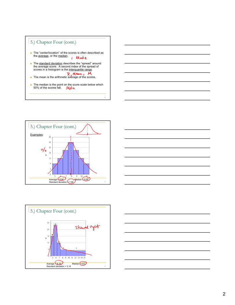
The “center/location” of the scores is often described as the average, or the median.

The standard deviation describes the “spread” around the average score. A second index of the spread of

4

g pscores in a histogram is the interquartile range.

The mean is the arithmetic average of the scores.

The median is the point on the score scale below which 50% of the scores fall.

5.) Chapter Four (cont.)Examples:

1 6

2 0

2 4

2 8

5

0

4

8

1 2

1 6%

5 6 7 8 9 10 11

Average = 8.00 Median = 8.00Standard deviation = 1.66

5.) Chapter Four (cont.)

1 8

2 4

3 0

18

28

6

0

6

1 2

%

5 6 7 8 9 10 11 12 13 14 15

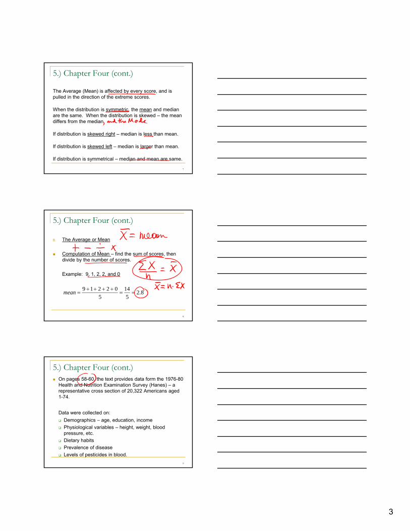
Average = 8.19 Median = 6.8Standard deviation = 3.14

12

6 5

3

5.) Chapter Four (cont.)

The Average (Mean) is affected by every score, and is pulled in the direction of the extreme scores.

When the distribution is symmetric, the mean and median are the same. When the distribution is skewed – the mean

7

differs from the median.

If distribution is skewed right – median is less than mean.

If distribution is skewed left – median is larger than mean.

If distribution is symmetrical – median and mean are same.

5.) Chapter Four (cont.)

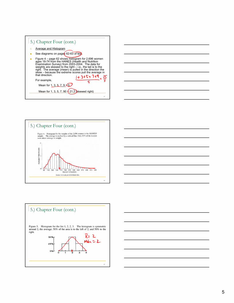
B. The Average or Mean

Computation of Mean – find the sum of scores, then divide by the number of scores.

8

Example: 9, 1, 2, 2, and 0

8.25

145

02219==

++++=mean

5.) Chapter Four (cont.)On pages 58-60, the text provides data form the 1976-80 Health and Nutrition Examination Survey (Hanes) – a representative cross section of 20,322 Americans aged 1-74.

Data were collected on:

9

Data were collected on:Demographics – age, education, incomePhysiological variables – height, weight, blood pressure, etc. Dietary habitsPrevalence of diseaseLevels of pesticides in blood.

4

5.) Chapter Four (cont.)

The plots of the average heights and weights by age in years for the 2003-04 survey are shown in Figure 3 (page 59).

10

A symbol for the average or the mean is commonly reported as , and the sum of scores is represented by

.

So, = which means to find the sum of all the scores, and then divide the sum by the total number of scores.

ΣΧx

nx /ΣΧ=

5.) Chapter Four (cont.)

11

5.) Chapter Four (cont.)

Exercise Set A – pp. 60-61 assign 1, 3, 8#4 N=10 avg=5 ft and 6 inches or 66 inches

This means the sum of their heights is 660 inches.

The 11th person is 6 feet 5 inches or 77 inches

12

The 11th person is 6 feet 5 inches or 77 inches.

The new sum would be 660 + 77 = 737 inches

The new mean would be inches or 5 feet and 7 inches.

6711737

=

5

5.) Chapter Four (cont.)C. Average and Histogram

See diagrams on pages 62-63 of text.

Figure 4 – page 62 shows histogram for 2,696 women ages 18-74 from the HANES (Health and Nutrition Examination Survey) from 2003-2004. The data for weights are skewed to the right – i e the tail is to the

13

weights are skewed to the right i.e., the tail is to the right. The average (mean) is pulled in the direction the skew – because the extreme scores pull the average in that direction.

For example,

Mean for 1, 3, 5, 7, 9 = 5

Mean for 1, 3, 5, 7, 90 = 21.2 (skewed right)

5.) Chapter Four (cont.)

14

5.) Chapter Four (cont.)

15

6

5.) Chapter Four (cont.)If the data for a histogram are skewed to the left (tail is at lower end of the histogram), the mean is pulled to the left.

Mean for 10, 12, 14, 16, 18 = 14

16

Mean for 1, 5, 14, 16, 18 = 10.8

The Mean is the point of balance in a distribution of scores – that is, the sum of the scores above the mean is equal to the sum of scores below the mean – the mean is a centroid.

( ) 0=−Σ xx

5.) Chapter Four (cont.)The sum of the differences between each score and the mean is always equal to zero.Example:

1, 3, 5, 7, 9

55

25ΣΧ

===

=ΣΧ

xmean

17

5( ) ( ) ( ) ( ) ( ) ( )( )( ) 0

)4()2()0()2()4(5957555351

=−Σ+++−+−=−Σ

−+−+−+−+−=−Σ

xxxxxx

The centroid (mean) for a seesaw (page 64) is such that it can be balanced by two persons of different weights by their distance from the centroid.

5.) Chapter Four (cont.)

18

7

5.) Chapter Four (cont.)

Median – as shown in histograms on page 64, the median has 50% of the scores (area) below the median, and 50% of the scores (area) above the median.

Symmetrical histogram – mean is same as median

19

y g

Skewed Right histogram – median is less than mean

Skewed Left histogram – median is greater than mean

See Exercise Set B (page 65) – 1, 2, 3, 4

5.) Chapter Four (cont.)

Computing mean in a Histogram

x f f · x19 1 1918 2 36

20

17 3 5116 4 6415 5 7514 6 8413 4 5212 3 3611 2 22

N=30 Sum=439

63.14=x

5.) Chapter Four (cont.)

Note: Again we assume each score has value of the midpoint of score interval.

21

For example: the 3 scores of 17 would be evenly distributed across the interval between 16.5 and 17.5

8

5.) Chapter Four (cont.)Computing mean in a grouped distribution –HISTOGRAM

x x midpt f f · x midpt18-20 19 2 3815-17 16 3 4812-14 13 4 52 227

=scoresofnumber

scoresofsumx

22

9-11 10 6 606-8 7 3 213-5 4 2 8

N=20 Sum ≈227

35.11

35.1120

227

≈

=≈

x

x

Assume: Scores in an interval evenly distributed throughout the score interval

f · midpt ≈ sum of scores in interval

5.) Chapter Four (cont.)

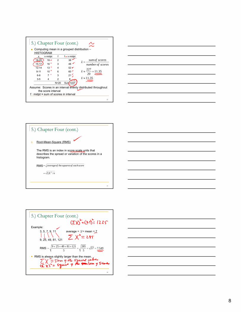
D. Root-Mean-Square (RMS)

The RMS is an index in score scale units that describes the spread or variation of the scores in a

23

histogram.

RMS scoreeachofsquarestheofaverage=

nX /2Σ=

5.) Chapter Four (cont.)

Example:3, 5, 7, 9, 11 average = = mean = 7

9, 25, 49, 81, 121

x

24

RMS

RMS is always slightly larger than the mean.

549.7575

2855

1218149259===

++++=