elementary linear algebra - mgmp matematika satap … › ... · elementary linear algebra k. r....
TRANSCRIPT
ELEMENTARY
LINEAR ALGEBRA
K. R. MATTHEWS
DEPARTMENT OF MATHEMATICS
UNIVERSITY OF QUEENSLAND
Corrected Version, 10th February 2010
Comments to the author at [email protected]
Contents
1 LINEAR EQUATIONS 1
1.1 Introduction to linear equations . . . . . . . . . . . . . . . . . 1
1.2 Solving linear equations . . . . . . . . . . . . . . . . . . . . . 5
1.3 The Gauss–Jordan algorithm . . . . . . . . . . . . . . . . . . 8
1.4 Systematic solution of linear systems. . . . . . . . . . . . . . 9
1.5 Homogeneous systems . . . . . . . . . . . . . . . . . . . . . . 16
1.6 PROBLEMS . . . . . . . . . . . . . . . . . . . . . . . . . . . 17
2 MATRICES 23
2.1 Matrix arithmetic . . . . . . . . . . . . . . . . . . . . . . . . . 23
2.2 Linear transformations . . . . . . . . . . . . . . . . . . . . . . 27
2.3 Recurrence relations . . . . . . . . . . . . . . . . . . . . . . . 31
2.4 PROBLEMS . . . . . . . . . . . . . . . . . . . . . . . . . . . 33
2.5 Non–singular matrices . . . . . . . . . . . . . . . . . . . . . . 36
2.6 Least squares solution of equations . . . . . . . . . . . . . . . 47
2.7 PROBLEMS . . . . . . . . . . . . . . . . . . . . . . . . . . . 49
3 SUBSPACES 55
3.1 Introduction . . . . . . . . . . . . . . . . . . . . . . . . . . . . 55
3.2 Subspaces of Fn . . . . . . . . . . . . . . . . . . . . . . . . . 55
3.3 Linear dependence . . . . . . . . . . . . . . . . . . . . . . . . 58
3.4 Basis of a subspace . . . . . . . . . . . . . . . . . . . . . . . . 61
3.5 Rank and nullity of a matrix . . . . . . . . . . . . . . . . . . 63
3.6 PROBLEMS . . . . . . . . . . . . . . . . . . . . . . . . . . . 67
4 DETERMINANTS 71
4.1 PROBLEMS . . . . . . . . . . . . . . . . . . . . . . . . . . . 84
i
5 COMPLEX NUMBERS 895.1 Constructing the complex numbers . . . . . . . . . . . . . . . 895.2 Calculating with complex numbers . . . . . . . . . . . . . . . 915.3 Geometric representation of C . . . . . . . . . . . . . . . . . . 955.4 Complex conjugate . . . . . . . . . . . . . . . . . . . . . . . . 965.5 Modulus of a complex number . . . . . . . . . . . . . . . . . 995.6 Argument of a complex number . . . . . . . . . . . . . . . . . 1035.7 De Moivre’s theorem . . . . . . . . . . . . . . . . . . . . . . . 1075.8 PROBLEMS . . . . . . . . . . . . . . . . . . . . . . . . . . . 111
6 EIGENVALUES AND EIGENVECTORS 1156.1 Motivation . . . . . . . . . . . . . . . . . . . . . . . . . . . . 1156.2 Definitions and examples . . . . . . . . . . . . . . . . . . . . . 1186.3 PROBLEMS . . . . . . . . . . . . . . . . . . . . . . . . . . . 124
7 Identifying second degree equations 1297.1 The eigenvalue method . . . . . . . . . . . . . . . . . . . . . . 1297.2 A classification algorithm . . . . . . . . . . . . . . . . . . . . 1417.3 PROBLEMS . . . . . . . . . . . . . . . . . . . . . . . . . . . 147
8 THREE–DIMENSIONAL GEOMETRY 1498.1 Introduction . . . . . . . . . . . . . . . . . . . . . . . . . . . . 1498.2 Three–dimensional space . . . . . . . . . . . . . . . . . . . . . 1548.3 Dot product . . . . . . . . . . . . . . . . . . . . . . . . . . . . 1568.4 Lines . . . . . . . . . . . . . . . . . . . . . . . . . . . . . . . . 1618.5 The angle between two vectors . . . . . . . . . . . . . . . . . 1668.6 The cross–product of two vectors . . . . . . . . . . . . . . . . 1728.7 Planes . . . . . . . . . . . . . . . . . . . . . . . . . . . . . . . 1768.8 PROBLEMS . . . . . . . . . . . . . . . . . . . . . . . . . . . 185
9 FURTHER READING 189
ii
List of Figures
1.1 Gauss–Jordan algorithm . . . . . . . . . . . . . . . . . . . . . 10
2.1 Reflection in a line . . . . . . . . . . . . . . . . . . . . . . . . 29
2.2 Projection on a line . . . . . . . . . . . . . . . . . . . . . . . 30
4.1 Area of triangle OPQ. . . . . . . . . . . . . . . . . . . . . . . 72
5.1 Complex addition and subtraction . . . . . . . . . . . . . . . 96
5.2 Complex conjugate . . . . . . . . . . . . . . . . . . . . . . . . 97
5.3 Modulus of a complex number . . . . . . . . . . . . . . . . . 99
5.4 Apollonius circles . . . . . . . . . . . . . . . . . . . . . . . . . 101
5.5 Argument of a complex number . . . . . . . . . . . . . . . . . 103
5.6 Argument examples . . . . . . . . . . . . . . . . . . . . . . . 105
5.7 The nth roots of unity. . . . . . . . . . . . . . . . . . . . . . . 108
5.8 The roots of zn = a. . . . . . . . . . . . . . . . . . . . . . . . 109
6.1 Rotating the axes . . . . . . . . . . . . . . . . . . . . . . . . . 116
7.1 An ellipse example . . . . . . . . . . . . . . . . . . . . . . . . 135
7.2 ellipse: standard form . . . . . . . . . . . . . . . . . . . . . . 137
7.3 hyperbola: standard forms . . . . . . . . . . . . . . . . . . . . 138
7.4 parabola: standard forms (i) and (ii) . . . . . . . . . . . . . . 138
7.5 parabola: standard forms (iii) and (iv) . . . . . . . . . . . . . 139
7.6 1st parabola example . . . . . . . . . . . . . . . . . . . . . . . 140
7.7 2nd parabola example . . . . . . . . . . . . . . . . . . . . . . 141
8.1 Equality and addition of vectors . . . . . . . . . . . . . . . . 150
8.2 Scalar multiplication of vectors. . . . . . . . . . . . . . . . . . 151
8.3 Representation of three–dimensional space . . . . . . . . . . . 155
8.4 The vector-
AB. . . . . . . . . . . . . . . . . . . . . . . . . . . 155
8.5 The negative of a vector. . . . . . . . . . . . . . . . . . . . . . 157
iii
8.6 (a) Equality of vectors; (b) Addition and subtraction of vectors.1578.7 Position vector as a linear combination of i, j and k. . . . . . 1588.8 Representation of a line. . . . . . . . . . . . . . . . . . . . . . 1628.9 The line AB. . . . . . . . . . . . . . . . . . . . . . . . . . . . 1628.10 The cosine rule for a triangle. . . . . . . . . . . . . . . . . . . 1678.11 Pythagoras’ theorem for a right–angled triangle. . . . . . . . 1688.12 Distance from a point to a line. . . . . . . . . . . . . . . . . . 1698.13 Projecting a segment onto a line. . . . . . . . . . . . . . . . . 1718.14 The vector cross–product. . . . . . . . . . . . . . . . . . . . . 1748.15 Vector equation for the plane ABC. . . . . . . . . . . . . . . 1778.16 Normal equation of the plane ABC. . . . . . . . . . . . . . . 1788.17 The plane ax + by + cz = d. . . . . . . . . . . . . . . . . . . . 1798.18 Line of intersection of two planes. . . . . . . . . . . . . . . . . 1828.19 Distance from a point to the plane ax + by + cz = d. . . . . . 184
iv
Chapter 1
LINEAR EQUATIONS
1.1 Introduction to linear equations
A linear equation in n unknowns x1, x2, · · · , xn is an equation of the form
a1x1 + a2x2 + · · · + anxn = b,
where a1, a2, . . . , an, b are given real numbers.
For example, with x and y instead of x1 and x2, the linear equation2x + 3y = 6 describes the line passing through the points (3, 0) and (0, 2).
Similarly, with x, y and z instead of x1, x2 and x3, the linear equa-tion 2x + 3y + 4z = 12 describes the plane passing through the points(6, 0, 0), (0, 4, 0), (0, 0, 3).
A system of m linear equations in n unknowns x1, x2, · · · , xn is a familyof linear equations
a11x1 + a12x2 + · · · + a1nxn = b1
a21x1 + a22x2 + · · · + a2nxn = b2
...
am1x1 + am2x2 + · · · + amnxn = bm.
We wish to determine if such a system has a solution, that is to findout if there exist numbers x1, x2, · · · , xn which satisfy each of the equationssimultaneously. We say that the system is consistent if it has a solution.Otherwise the system is called inconsistent.
1
2 CHAPTER 1. LINEAR EQUATIONS
Note that the above system can be written concisely as
n∑
j=1
aijxj = bi, i = 1, 2, · · · , m.
The matrix
a11 a12 · · · a1n
a21 a22 · · · a2n...
...am1 am2 · · · amn
is called the coefficient matrix of the system, while the matrix
a11 a12 · · · a1n b1
a21 a22 · · · a2n b2...
......
am1 am2 · · · amn bm
is called the augmented matrix of the system.
Geometrically, solving a system of linear equations in two (or three)unknowns is equivalent to determining whether or not a family of lines (orplanes) has a common point of intersection.
EXAMPLE 1.1.1 Solve the equation
2x + 3y = 6.
Solution. The equation 2x + 3y = 6 is equivalent to 2x = 6 − 3y orx = 3 − 3
2y, where y is arbitrary. So there are infinitely many solutions.
EXAMPLE 1.1.2 Solve the system
x + y + z = 1
x − y + z = 0.
Solution. We subtract the second equation from the first, to get 2y = 1and y = 1
2 . Then x = y − z = 12 − z, where z is arbitrary. Again there are
infinitely many solutions.
EXAMPLE 1.1.3 Find a polynomial of the form y = a0+a1x+a2x2+a3x
3
which passes through the points (−3, −2), (−1, 2), (1, 5), (2, 1).
1.1. INTRODUCTION TO LINEAR EQUATIONS 3
Solution. When x has the values −3, −1, 1, 2, then y takes correspondingvalues −2, 2, 5, 1 and we get four equations in the unknowns a0, a1, a2, a3:
a0 − 3a1 + 9a2 − 27a3 = −2
a0 − a1 + a2 − a3 = 2
a0 + a1 + a2 + a3 = 5
a0 + 2a1 + 4a2 + 8a3 = 1,
with unique solution a0 = 93/20, a1 = 221/120, a2 = −23/20, a3 = −41/120.So the required polynomial is
y =93
20+
221
120x − 23
20x2 − 41
120x3.
In [26, pages 33–35] there are examples of systems of linear equationswhich arise from simple electrical networks using Kirchhoff’s laws for elec-trical circuits.
Solving a system consisting of a single linear equation is easy. However ifwe are dealing with two or more equations, it is desirable to have a systematicmethod of determining if the system is consistent and to find all solutions.
Instead of restricting ourselves to linear equations with rational or realcoefficients, our theory goes over to the more general case where the coef-ficients belong to an arbitrary field. A field F is a set F which possessesoperations of addition and multiplication which satisfy the familiar rules ofrational arithmetic. There are ten basic properties that a field must have:
THE FIELD AXIOMS.
1. (a + b) + c = a + (b + c) for all a, b, c in F ;
2. (ab)c = a(bc) for all a, b, c in F ;
3. a + b = b + a for all a, b in F ;
4. ab = ba for all a, b in F ;
5. there exists an element 0 in F such that 0 + a = a for all a in F ;
6. there exists an element 1 in F such that 1a = a for all a in F ;
7. to every a in F , there corresponds an additive inverse −a in F , satis-fying
a + (−a) = 0;
4 CHAPTER 1. LINEAR EQUATIONS
8. to every non–zero a in F , there corresponds a multiplicative inverse
a−1 in F , satisfying
aa−1 = 1;
9. a(b + c) = ab + ac for all a, b, c in F ;
10. 0 6= 1.
With standard definitions such as a − b = a + (−b) anda
b= ab−1 for
b 6= 0, we have the following familiar rules:
−(a + b) = (−a) + (−b), (ab)−1 = a−1b−1;
−(−a) = a, (a−1)−1 = a;
−(a − b) = b − a, (a
b)−1 =
b
a;
a
b+
c
d=
ad + bc
bd;
a
b
c
d=
ac
bd;
ab
ac=
b
c,
a(
bc
) =ac
b;
−(ab) = (−a)b = a(−b);
−(a
b
)
=−a
b=
a
−b;
0a = 0;
(−a)−1 = −(a−1).
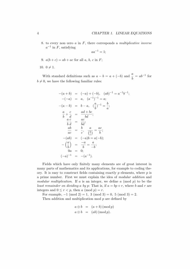
Fields which have only finitely many elements are of great interest inmany parts of mathematics and its applications, for example to coding the-ory. It is easy to construct fields containing exactly p elements, where p isa prime number. First we must explain the idea of modular addition andmodular multiplication. If a is an integer, we define a (mod p) to be theleast remainder on dividing a by p: That is, if a = bp + r, where b and r areintegers and 0 ≤ r < p, then a (mod p) = r.
For example, −1 (mod 2) = 1, 3 (mod 3) = 0, 5 (mod 3) = 2.
Then addition and multiplication mod p are defined by
a ⊕ b = (a + b) (mod p)
a ⊗ b = (ab) (mod p).
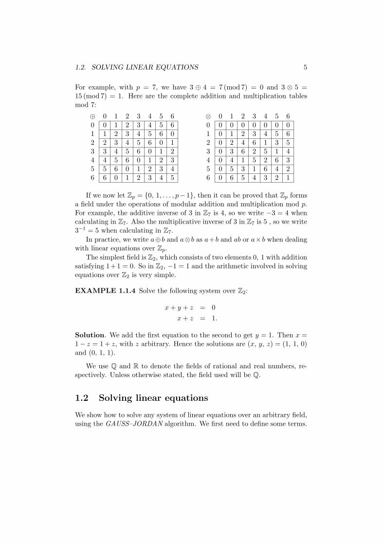
1.2. SOLVING LINEAR EQUATIONS 5
For example, with p = 7, we have 3 ⊕ 4 = 7 (mod 7) = 0 and 3 ⊗ 5 =15 (mod 7) = 1. Here are the complete addition and multiplication tablesmod 7:
⊕ 0 1 2 3 4 5 60 0 1 2 3 4 5 61 1 2 3 4 5 6 02 2 3 4 5 6 0 13 3 4 5 6 0 1 24 4 5 6 0 1 2 35 5 6 0 1 2 3 46 6 0 1 2 3 4 5
⊗ 0 1 2 3 4 5 60 0 0 0 0 0 0 01 0 1 2 3 4 5 62 0 2 4 6 1 3 53 0 3 6 2 5 1 44 0 4 1 5 2 6 35 0 5 3 1 6 4 26 0 6 5 4 3 2 1
If we now let Zp = {0, 1, . . . , p− 1}, then it can be proved that Zp formsa field under the operations of modular addition and multiplication mod p.For example, the additive inverse of 3 in Z7 is 4, so we write −3 = 4 whencalculating in Z7. Also the multiplicative inverse of 3 in Z7 is 5 , so we write3−1 = 5 when calculating in Z7.
In practice, we write a⊕b and a⊗b as a+b and ab or a×b when dealingwith linear equations over Zp.
The simplest field is Z2, which consists of two elements 0, 1 with additionsatisfying 1+1 = 0. So in Z2, −1 = 1 and the arithmetic involved in solvingequations over Z2 is very simple.
EXAMPLE 1.1.4 Solve the following system over Z2:
x + y + z = 0
x + z = 1.
Solution. We add the first equation to the second to get y = 1. Then x =1− z = 1 + z, with z arbitrary. Hence the solutions are (x, y, z) = (1, 1, 0)and (0, 1, 1).
We use Q and R to denote the fields of rational and real numbers, re-spectively. Unless otherwise stated, the field used will be Q.
1.2 Solving linear equations
We show how to solve any system of linear equations over an arbitrary field,using the GAUSS–JORDAN algorithm. We first need to define some terms.
6 CHAPTER 1. LINEAR EQUATIONS
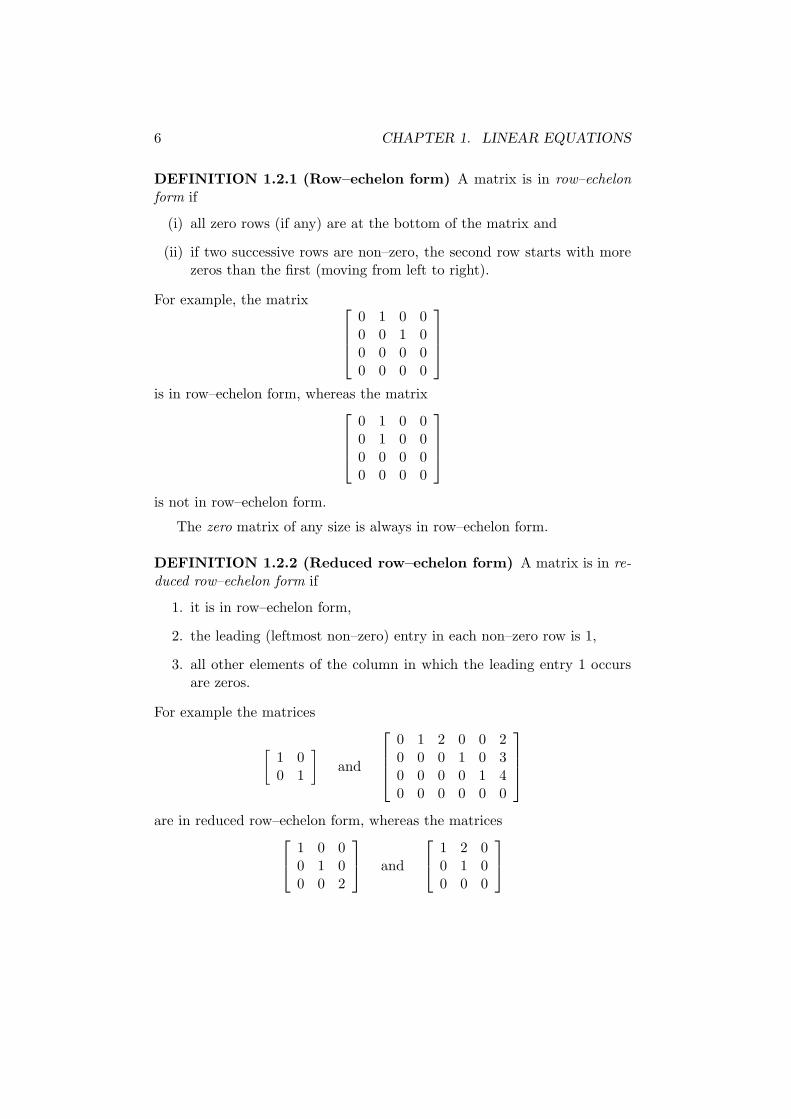
DEFINITION 1.2.1 (Row–echelon form) A matrix is in row–echelon
form if
(i) all zero rows (if any) are at the bottom of the matrix and
(ii) if two successive rows are non–zero, the second row starts with morezeros than the first (moving from left to right).
For example, the matrix
0 1 0 00 0 1 00 0 0 00 0 0 0
is in row–echelon form, whereas the matrix
0 1 0 00 1 0 00 0 0 00 0 0 0
is not in row–echelon form.
The zero matrix of any size is always in row–echelon form.
DEFINITION 1.2.2 (Reduced row–echelon form) A matrix is in re-
duced row–echelon form if
1. it is in row–echelon form,
2. the leading (leftmost non–zero) entry in each non–zero row is 1,
3. all other elements of the column in which the leading entry 1 occursare zeros.
For example the matrices
[
1 00 1
]
and
0 1 2 0 0 20 0 0 1 0 30 0 0 0 1 40 0 0 0 0 0
are in reduced row–echelon form, whereas the matrices
1 0 00 1 00 0 2
and
1 2 00 1 00 0 0
1.2. SOLVING LINEAR EQUATIONS 7
are not in reduced row–echelon form, but are in row–echelon form.
The zero matrix of any size is always in reduced row–echelon form.
Notation. If a matrix is in reduced row–echelon form, it is useful to denotethe column numbers in which the leading entries 1 occur, by c1, c2, . . . , cr,with the remaining column numbers being denoted by cr+1, . . . , cn, wherer is the number of non–zero rows. For example, in the 4 × 6 matrix above,we have r = 3, c1 = 2, c2 = 4, c3 = 5, c4 = 1, c5 = 3, c6 = 6.
The following operations are the ones used on systems of linear equationsand do not change the solutions.
DEFINITION 1.2.3 (Elementary row operations) Three types of el-
ementary row operations can be performed on matrices:
1. Interchanging two rows:
Ri ↔ Rj interchanges rows i and j.
2. Multiplying a row by a non–zero scalar:
Ri → tRi multiplies row i by the non–zero scalar t.
3. Adding a multiple of one row to another row:
Rj → Rj + tRi adds t times row i to row j.
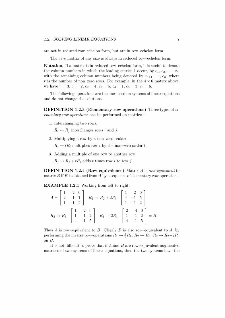
DEFINITION 1.2.4 (Row equivalence) Matrix A is row–equivalent tomatrix B if B is obtained from A by a sequence of elementary row operations.
EXAMPLE 1.2.1 Working from left to right,
A =
1 2 02 1 11 −1 2
R2 → R2 + 2R3
1 2 04 −1 51 −1 2
R2 ↔ R3
1 2 01 −1 24 −1 5
R1 → 2R1
2 4 01 −1 24 −1 5
= B.
Thus A is row–equivalent to B. Clearly B is also row–equivalent to A, byperforming the inverse row–operations R1 → 1
2R1, R2 ↔ R3, R2 → R2−2R3
on B.It is not difficult to prove that if A and B are row–equivalent augmented
matrices of two systems of linear equations, then the two systems have the
8 CHAPTER 1. LINEAR EQUATIONS
same solution sets – a solution of the one system is a solution of the other.For example the systems whose augmented matrices are A and B in theabove example are respectively
x + 2y = 02x + y = 1x − y = 2
and
2x + 4y = 0x − y = 2
4x − y = 5
and these systems have precisely the same solutions.
1.3 The Gauss–Jordan algorithm
We now describe the GAUSS–JORDAN ALGORITHM. This is a processwhich starts with a given matrix A and produces a matrix B in reduced row–echelon form, which is row–equivalent to A. If A is the augmented matrixof a system of linear equations, then B will be a much simpler matrix thanA from which the consistency or inconsistency of the corresponding systemis immediately apparent and in fact the complete solution of the system canbe read off.
STEP 1.Find the first non–zero column moving from left to right, (column c1)
and select a non–zero entry from this column. By interchanging rows, ifnecessary, ensure that the first entry in this column is non–zero. Multiplyrow 1 by the multiplicative inverse of a1c1 thereby converting a1c1 to 1. Foreach non–zero element aic1 , i > 1, (if any) in column c1, add −aic1 timesrow 1 to row i, thereby ensuring that all elements in column c1, apart fromthe first, are zero.
STEP 2. If the matrix obtained at Step 1 has its 2nd, . . . , mth rows allzero, the matrix is in reduced row–echelon form. Otherwise suppose thatthe first column which has a non–zero element in the rows below the first iscolumn c2. Then c1 < c2. By interchanging rows below the first, if necessary,ensure that a2c2 is non–zero. Then convert a2c2 to 1 and by adding suitablemultiples of row 2 to the remaing rows, where necessary, ensure that allremaining elements in column c2 are zero.
The process is repeated and will eventually stop after r steps, eitherbecause we run out of rows, or because we run out of non–zero columns. Ingeneral, the final matrix will be in reduced row–echelon form and will haver non–zero rows, with leading entries 1 in columns c1, . . . , cr, respectively.
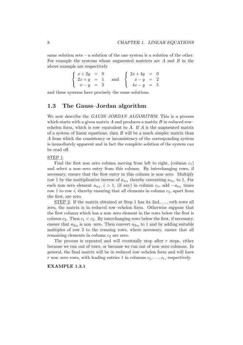
EXAMPLE 1.3.1
1.4. SYSTEMATIC SOLUTION OF LINEAR SYSTEMS. 9
0 0 4 02 2 −2 55 5 −1 5
R1 ↔ R2
2 2 −2 50 0 4 05 5 −1 5
R1 → 12R1
1 1 −1 52
0 0 4 05 5 −1 5
R3 → R3 − 5R1
1 1 −1 52
0 0 4 00 0 4 −15
2
R2 → 14R2
1 1 −1 52
0 0 1 00 0 4 −15
2
{
R1 → R1 + R2
R3 → R3 − 4R2
1 1 0 52
0 0 1 00 0 0 −15
2
R3 → −215 R3
1 1 0 52
0 0 1 00 0 0 1
R1 → R1 − 52R3
1 1 0 00 0 1 00 0 0 1
The last matrix is in reduced row–echelon form.
REMARK 1.3.1 It is possible to show that a given matrix over an ar-bitrary field is row–equivalent to precisely one matrix which is in reducedrow–echelon form.
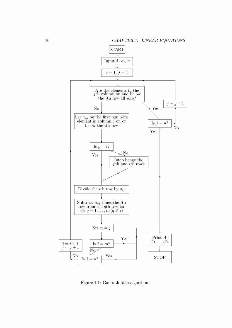
A flow–chart for the Gauss–Jordan algorithm, based on [1, page 83] is pre-sented in figure 1.1 below.
1.4 Systematic solution of linear systems.
Suppose a system of m linear equations in n unknowns x1, · · · , xn has aug-mented matrix A and that A is row–equivalent to a matrix B which is inreduced row–echelon form, via the Gauss–Jordan algorithm. Then A and Bare m × (n + 1). Suppose that B has r non–zero rows and that the leadingentry 1 in row i occurs in column number ci, for 1 ≤ i ≤ r. Then
1 ≤ c1 < c2 < · · · , < cr ≤ n + 1.
Also assume that the remaining column numbers are cr+1, · · · , cn+1, where
1 ≤ cr+1 < cr+2 < · · · < cn ≤ n + 1.
Case 1: cr = n + 1. The system is inconsistent. For the last non–zerorow of B is [0, 0, · · · , 1] and the corresponding equation is
0x1 + 0x2 + · · · + 0xn = 1,
10 CHAPTER 1. LINEAR EQUATIONS
START
?InputA, m, n
?i = 1, j = 1
?- ¾
?Are the elements in the
jth column on and belowthe ith row all zero?
j = j + 1@@
@@@
R YesNo?
Is j = n?
YesNo
-
6
Let apj be the first non–zeroelement in column j on or
below the ith row
?Is p = i?
Yes
?
PPPPPq No
Interchange thepth and ith rows
©©©©©©©
¼
Divide the ith row by aij
?Subtract aqj times the ithrow from the qth row forfor q = 1, . . . , m (q 6= i)
?Set ci = j
?Is i = m?
´´
+Is j = n?¾
i = i + 1j = j + 1
6
No
No
Yes
Yes -
-6
?
Print A,c1, . . . , ci
?
STOP
Figure 1.1: Gauss–Jordan algorithm.
1.4. SYSTEMATIC SOLUTION OF LINEAR SYSTEMS. 11
which has no solutions. Consequently the original system has no solutions.
Case 2: cr ≤ n. The system of equations corresponding to the non–zerorows of B is consistent. First notice that r ≤ n here.
If r = n, then c1 = 1, c2 = 2, · · · , cn = n and
B =
1 0 · · · 0 d1
0 1 · · · 0 d2...
...0 0 · · · 1 dn
0 0 · · · 0 0...
...0 0 · · · 0 0
.
There is a unique solution x1 = d1, x2 = d2, · · · , xn = dn.
If r < n, there will be more than one solution (infinitely many if thefield is infinite). For all solutions are obtained by taking the unknownsxc1 , · · · , xcr as dependent unknowns and using the r equations correspond-ing to the non–zero rows of B to express these unknowns in terms of theremaining independent unknowns xcr+1 , . . . , xcn , which can take on arbi-trary values:
xc1 = b1 n+1 − b1cr+1xcr+1 − · · · − b1cnxcn
...
xcr = br n+1 − brcr+1xcr+1 − · · · − brcnxcn .
In particular, taking xcr+1 = 0, . . . , xcn−1 = 0 and xcn = 0, 1 respectively,produces at least two solutions.
EXAMPLE 1.4.1 Solve the system
x + y = 0
x − y = 1
4x + 2y = 1.
Solution. The augmented matrix of the system is
A =
1 1 01 −1 14 2 1
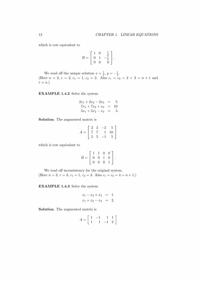
12 CHAPTER 1. LINEAR EQUATIONS
which is row equivalent to
B =
1 0 12
0 1 −12
0 0 0
.
We read off the unique solution x = 12 , y = −1
2 .
(Here n = 2, r = 2, c1 = 1, c2 = 2. Also cr = c2 = 2 < 3 = n + 1 andr = n.)
EXAMPLE 1.4.2 Solve the system
2x1 + 2x2 − 2x3 = 57x1 + 7x2 + x3 = 105x1 + 5x2 − x3 = 5.
Solution. The augmented matrix is
A =
2 2 −2 57 7 1 105 5 −1 5
which is row equivalent to
B =
1 1 0 00 0 1 00 0 0 1
.
We read off inconsistency for the original system.
(Here n = 3, r = 3, c1 = 1, c2 = 3. Also cr = c3 = 4 = n + 1.)
EXAMPLE 1.4.3 Solve the system
x1 − x2 + x3 = 1
x1 + x2 − x3 = 2.
Solution. The augmented matrix is
A =
[
1 −1 1 11 1 −1 2
]
1.4. SYSTEMATIC SOLUTION OF LINEAR SYSTEMS. 13
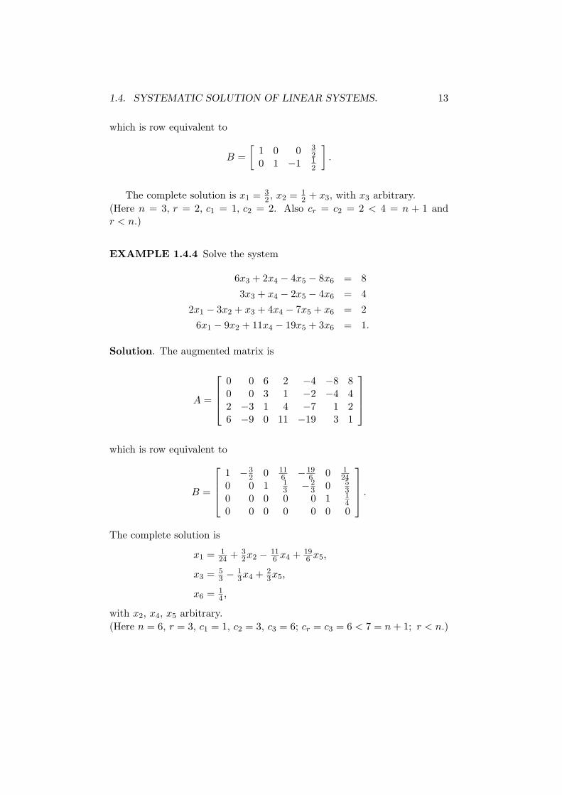
which is row equivalent to
B =
[
1 0 0 32
0 1 −1 12
]
.
The complete solution is x1 = 32 , x2 = 1
2 + x3, with x3 arbitrary.
(Here n = 3, r = 2, c1 = 1, c2 = 2. Also cr = c2 = 2 < 4 = n + 1 andr < n.)
EXAMPLE 1.4.4 Solve the system
6x3 + 2x4 − 4x5 − 8x6 = 8
3x3 + x4 − 2x5 − 4x6 = 4
2x1 − 3x2 + x3 + 4x4 − 7x5 + x6 = 2
6x1 − 9x2 + 11x4 − 19x5 + 3x6 = 1.
Solution. The augmented matrix is
A =
0 0 6 2 −4 −8 80 0 3 1 −2 −4 42 −3 1 4 −7 1 26 −9 0 11 −19 3 1
which is row equivalent to
B =
1 −32 0 11
6 −196 0 1
240 0 1 1
3 −23 0 5
30 0 0 0 0 1 1
40 0 0 0 0 0 0
.
The complete solution is
x1 = 124 + 3
2x2 − 116 x4 + 19
6 x5,
x3 = 53 − 1
3x4 + 23x5,
x6 = 14 ,
with x2, x4, x5 arbitrary.
(Here n = 6, r = 3, c1 = 1, c2 = 3, c3 = 6; cr = c3 = 6 < 7 = n + 1; r < n.)

14 CHAPTER 1. LINEAR EQUATIONS
EXAMPLE 1.4.5 Find the rational number t for which the following sys-tem is consistent and solve the system for this value of t.
x + y = 2
x − y = 0
3x − y = t.
Solution. The augmented matrix of the system is
A =
1 1 21 −1 03 −1 t
which is row–equivalent to the simpler matrix
B =
1 1 20 1 10 0 t − 2
.
Hence if t 6= 2 the system is inconsistent. If t = 2 the system is consistentand
B =
1 1 20 1 10 0 0
→
1 0 10 1 10 0 0
.
We read off the solution x = 1, y = 1.
EXAMPLE 1.4.6 For which rationals a and b does the following systemhave (i) no solution, (ii) a unique solution, (iii) infinitely many solutions?
x − 2y + 3z = 4
2x − 3y + az = 5
3x − 4y + 5z = b.
Solution. The augmented matrix of the system is
A =
1 −2 3 42 −3 a 53 −4 5 b
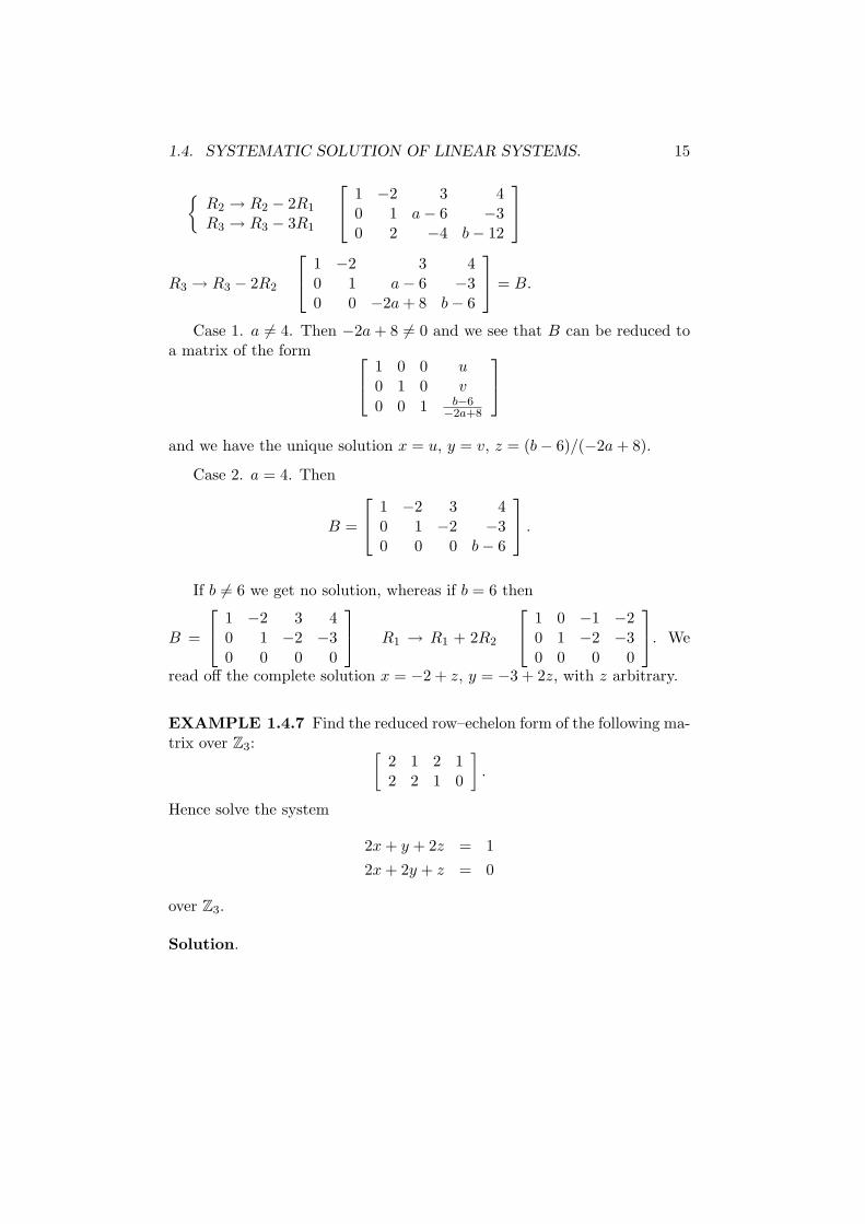
1.4. SYSTEMATIC SOLUTION OF LINEAR SYSTEMS. 15
{
R2 → R2 − 2R1
R3 → R3 − 3R1
1 −2 3 40 1 a − 6 −30 2 −4 b − 12
R3 → R3 − 2R2
1 −2 3 40 1 a − 6 −30 0 −2a + 8 b − 6
= B.
Case 1. a 6= 4. Then −2a + 8 6= 0 and we see that B can be reduced toa matrix of the form
1 0 0 u0 1 0 v
0 0 1 b−6−2a+8
and we have the unique solution x = u, y = v, z = (b − 6)/(−2a + 8).
Case 2. a = 4. Then
B =
1 −2 3 40 1 −2 −30 0 0 b − 6
.
If b 6= 6 we get no solution, whereas if b = 6 then
B =
1 −2 3 40 1 −2 −30 0 0 0
R1 → R1 + 2R2
1 0 −1 −20 1 −2 −30 0 0 0
. We
read off the complete solution x = −2 + z, y = −3 + 2z, with z arbitrary.
EXAMPLE 1.4.7 Find the reduced row–echelon form of the following ma-trix over Z3:
[
2 1 2 12 2 1 0
]
.
Hence solve the system
2x + y + 2z = 1
2x + 2y + z = 0
over Z3.
Solution.
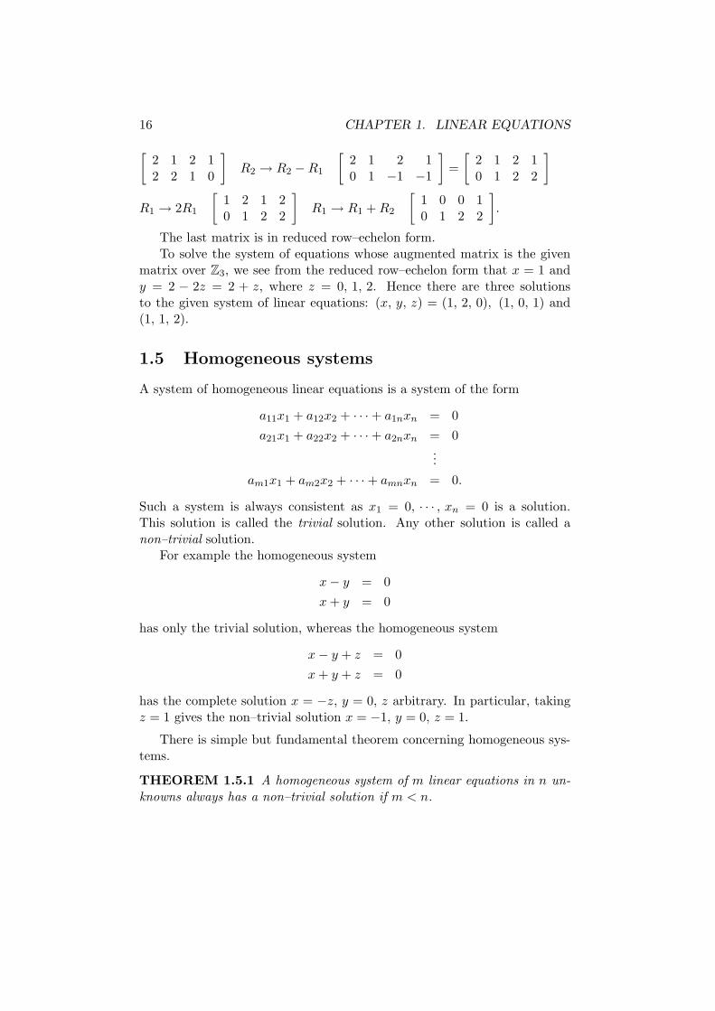
16 CHAPTER 1. LINEAR EQUATIONS
[
2 1 2 12 2 1 0
]
R2 → R2 − R1
[
2 1 2 10 1 −1 −1
]
=
[
2 1 2 10 1 2 2
]
R1 → 2R1
[
1 2 1 20 1 2 2
]
R1 → R1 + R2
[
1 0 0 10 1 2 2
]
.
The last matrix is in reduced row–echelon form.To solve the system of equations whose augmented matrix is the given
matrix over Z3, we see from the reduced row–echelon form that x = 1 andy = 2 − 2z = 2 + z, where z = 0, 1, 2. Hence there are three solutionsto the given system of linear equations: (x, y, z) = (1, 2, 0), (1, 0, 1) and(1, 1, 2).
1.5 Homogeneous systems
A system of homogeneous linear equations is a system of the form
a11x1 + a12x2 + · · · + a1nxn = 0
a21x1 + a22x2 + · · · + a2nxn = 0...
am1x1 + am2x2 + · · · + amnxn = 0.
Such a system is always consistent as x1 = 0, · · · , xn = 0 is a solution.This solution is called the trivial solution. Any other solution is called anon–trivial solution.
For example the homogeneous system
x − y = 0
x + y = 0
has only the trivial solution, whereas the homogeneous system
x − y + z = 0
x + y + z = 0
has the complete solution x = −z, y = 0, z arbitrary. In particular, takingz = 1 gives the non–trivial solution x = −1, y = 0, z = 1.
There is simple but fundamental theorem concerning homogeneous sys-tems.
THEOREM 1.5.1 A homogeneous system of m linear equations in n un-
knowns always has a non–trivial solution if m < n.
1.6. PROBLEMS 17
Proof. Suppose that m < n and that the coefficient matrix of the systemis row–equivalent to B, a matrix in reduced row–echelon form. Let r be thenumber of non–zero rows in B. Then r ≤ m < n and hence n − r > 0 andso the number n − r of arbitrary unknowns is in fact positive. Taking oneof these unknowns to be 1 gives a non–trivial solution.
REMARK 1.5.1 Let two systems of homogeneous equations in n un-knowns have coefficient matrices A and B, respectively. If each row of B isa linear combination of the rows of A (i.e. a sum of multiples of the rowsof A) and each row of A is a linear combination of the rows of B, then it iseasy to prove that the two systems have identical solutions. The converse istrue, but is not easy to prove. Similarly if A and B have the same reducedrow–echelon form, apart from possibly zero rows, then the two systems haveidentical solutions and conversely.
There is a similar situation in the case of two systems of linear equations(not necessarily homogeneous), with the proviso that in the statement ofthe converse, the extra condition that both the systems are consistent, isneeded.
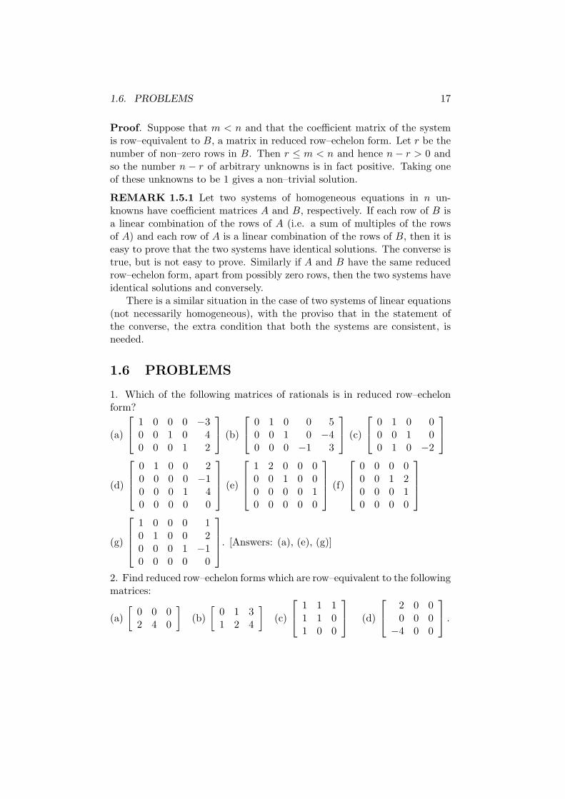
1.6 PROBLEMS
1. Which of the following matrices of rationals is in reduced row–echelonform?
(a)
1 0 0 0 −30 0 1 0 40 0 0 1 2
(b)
0 1 0 0 50 0 1 0 −40 0 0 −1 3
(c)
0 1 0 00 0 1 00 1 0 −2
(d)
0 1 0 0 20 0 0 0 −10 0 0 1 40 0 0 0 0
(e)
1 2 0 0 00 0 1 0 00 0 0 0 10 0 0 0 0
(f)
0 0 0 00 0 1 20 0 0 10 0 0 0
(g)
1 0 0 0 10 1 0 0 20 0 0 1 −10 0 0 0 0
. [Answers: (a), (e), (g)]
2. Find reduced row–echelon forms which are row–equivalent to the followingmatrices:
(a)
[
0 0 02 4 0
]
(b)
[
0 1 31 2 4
]
(c)
1 1 11 1 01 0 0
(d)
2 0 00 0 0
−4 0 0
.
18 CHAPTER 1. LINEAR EQUATIONS
[Answers:
(a)
[
1 2 00 0 0
]
(b)
[
1 0 −20 1 3
]
(c)
1 0 00 1 00 0 1
(d)
1 0 00 0 00 0 0
.]
3. Solve the following systems of linear equations by reducing the augmentedmatrix to reduced row–echelon form:
(a) x + y + z = 2 (b) x1 + x2 − x3 + 2x4 = 102x + 3y − z = 8 3x1 − x2 + 7x3 + 4x4 = 1
x − y − z = −8 −5x1 + 3x2 − 15x3 − 6x4 = 9
(c) 3x − y + 7z = 0 (d) 2x2 + 3x3 − 4x4 = 12x − y + 4z = 1
2 2x3 + 3x4 = 4x − y + z = 1 2x1 + 2x2 − 5x3 + 2x4 = 4
6x − 4y + 10z = 3 2x1 − 6x3 + 9x4 = 7
[Answers: (a) x = −3, y = 194 , z = 1
4 ; (b) inconsistent;
(c) x = −12 − 3z, y = −3
2 − 2z, with z arbitrary;
(d) x1 = 192 − 9x4, x2 = −5
2 + 174 x4, x3 = 2 − 3
2x4, with x4 arbitrary.]
4. Show that the following system is consistent if and only if c = 2a − 3band solve the system in this case.
2x − y + 3z = a
3x + y − 5z = b
−5x − 5y + 21z = c.
[Answer: x = a+b5 + 2
5z, y = −3a+2b5 + 19
5 z, with z arbitrary.]
5. Find the value of t for which the following system is consistent and solvethe system for this value of t.
x + y = 1
tx + y = t
(1 + t)x + 2y = 3.
[Answer: t = 2; x = 1, y = 0.]
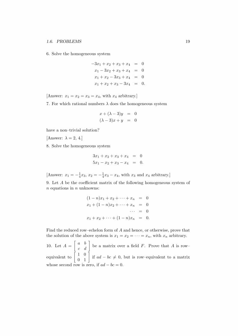
1.6. PROBLEMS 19
6. Solve the homogeneous system
−3x1 + x2 + x3 + x4 = 0
x1 − 3x2 + x3 + x4 = 0
x1 + x2 − 3x3 + x4 = 0
x1 + x2 + x3 − 3x4 = 0.
[Answer: x1 = x2 = x3 = x4, with x4 arbitrary.]
7. For which rational numbers λ does the homogeneous system
x + (λ − 3)y = 0
(λ − 3)x + y = 0
have a non–trivial solution?
[Answer: λ = 2, 4.]
8. Solve the homogeneous system
3x1 + x2 + x3 + x4 = 0
5x1 − x2 + x3 − x4 = 0.
[Answer: x1 = −14x3, x2 = −1
4x3 − x4, with x3 and x4 arbitrary.]
9. Let A be the coefficient matrix of the following homogeneous system ofn equations in n unknowns:
(1 − n)x1 + x2 + · · · + xn = 0
x1 + (1 − n)x2 + · · · + xn = 0
· · · = 0
x1 + x2 + · · · + (1 − n)xn = 0.
Find the reduced row–echelon form of A and hence, or otherwise, prove thatthe solution of the above system is x1 = x2 = · · · = xn, with xn arbitrary.
10. Let A =
[
a bc d
]
be a matrix over a field F . Prove that A is row–
equivalent to
[
1 00 1
]
if ad − bc 6= 0, but is row–equivalent to a matrix
whose second row is zero, if ad − bc = 0.

20 CHAPTER 1. LINEAR EQUATIONS
11. For which rational numbers a does the following system have (i) nosolutions (ii) exactly one solution (iii) infinitely many solutions?
x + 2y − 3z = 4
3x − y + 5z = 2
4x + y + (a2 − 14)z = a + 2.
[Answer: a = −4, no solution; a = 4, infinitely many solutions; a 6= ±4,exactly one solution.]
12. Solve the following system of homogeneous equations over Z2:
x1 + x3 + x5 = 0
x2 + x4 + x5 = 0
x1 + x2 + x3 + x4 = 0
x3 + x4 = 0.
[Answer: x1 = x2 = x4 + x5, x3 = x4, with x4 and x5 arbitrary elements ofZ2.]
13. Solve the following systems of linear equations over Z5:
(a) 2x + y + 3z = 4 (b) 2x + y + 3z = 44x + y + 4z = 1 4x + y + 4z = 13x + y + 2z = 0 x + y = 3.
[Answer: (a) x = 1, y = 2, z = 0; (b) x = 1 + 2z, y = 2 + 3z, with z anarbitrary element of Z5.]
14. If (α1, . . . , αn) and (β1, . . . , βn) are solutions of a system of linear equa-tions, prove that
((1 − t)α1 + tβ1, . . . , (1 − t)αn + tβn)
is also a solution.
15. If (α1, . . . , αn) is a solution of a system of linear equations, prove thatthe complete solution is given by x1 = α1 + y1, . . . , xn = αn + yn, where(y1, . . . , yn) is the general solution of the associated homogeneous system.
1.6. PROBLEMS 21
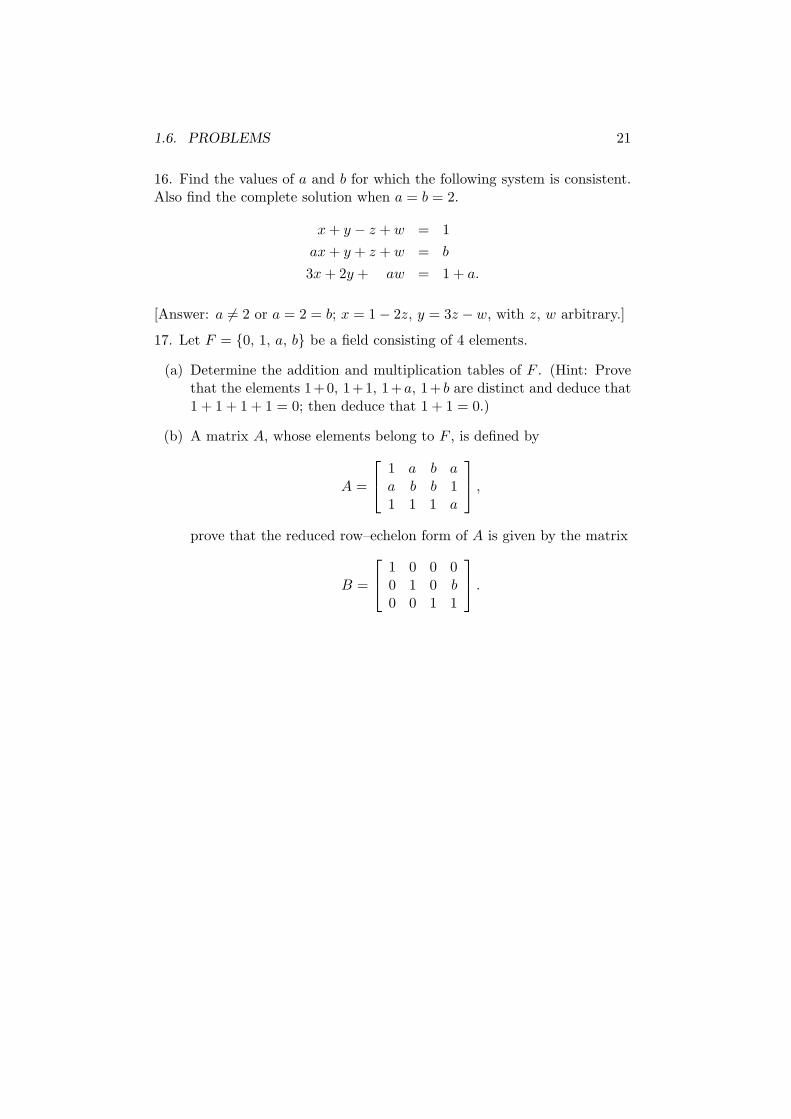
16. Find the values of a and b for which the following system is consistent.Also find the complete solution when a = b = 2.
x + y − z + w = 1
ax + y + z + w = b
3x + 2y + aw = 1 + a.
[Answer: a 6= 2 or a = 2 = b; x = 1 − 2z, y = 3z − w, with z, w arbitrary.]
17. Let F = {0, 1, a, b} be a field consisting of 4 elements.
(a) Determine the addition and multiplication tables of F . (Hint: Provethat the elements 1+0, 1+1, 1+a, 1+ b are distinct and deduce that1 + 1 + 1 + 1 = 0; then deduce that 1 + 1 = 0.)
(b) A matrix A, whose elements belong to F , is defined by
A =
1 a b aa b b 11 1 1 a
,
prove that the reduced row–echelon form of A is given by the matrix
B =
1 0 0 00 1 0 b0 0 1 1
.
22 CHAPTER 1. LINEAR EQUATIONS
Chapter 2
MATRICES
2.1 Matrix arithmetic
A matrix over a field F is a rectangular array of elements from F . The sym-bol Mm×n(F ) denotes the collection of all m× n matrices over F . Matriceswill usually be denoted by capital letters and the equation A = [aij ] meansthat the element in the i–th row and j–th column of the matrix A equalsaij . It is also occasionally convenient to write aij = (A)ij . For the present,all matrices will have rational entries, unless otherwise stated.
EXAMPLE 2.1.1 The formula aij = 1/(i + j) for 1 ≤ i ≤ 3, 1 ≤ j ≤ 4defines a 3 × 4 matrix A = [aij ], namely
A =
12
13
14
15
13
14
15
16
14
15
16
17
.
DEFINITION 2.1.1 (Equality of matrices) Matrices A, B are said tobe equal if A and B have the same size and corresponding elements areequal; i.e., A and B ∈ Mm×n(F ) and A = [aij ], B = [bij ], with aij = bij for1 ≤ i ≤ m, 1 ≤ j ≤ n.
DEFINITION 2.1.2 (Addition of matrices) Let A = [aij ] and B =[bij ] be of the same size. Then A + B is the matrix obtained by addingcorresponding elements of A and B; that is
A + B = [aij ] + [bij ] = [aij + bij ].
23
24 CHAPTER 2. MATRICES
DEFINITION 2.1.3 (Scalar multiple of a matrix) Let A = [aij ] andt ∈ F (that is t is a scalar). Then tA is the matrix obtained by multiplyingall elements of A by t; that is
tA = t[aij ] = [taij ].
DEFINITION 2.1.4 (Additive inverse of a matrix) Let A = [aij ] .Then −A is the matrix obtained by replacing the elements of A by theiradditive inverses; that is
−A = −[aij ] = [−aij ].
DEFINITION 2.1.5 (Subtraction of matrices) Matrix subtraction isdefined for two matrices A = [aij ] and B = [bij ] of the same size, in theusual way; that is
A − B = [aij ] − [bij ] = [aij − bij ].
DEFINITION 2.1.6 (The zero matrix) For each m, n the matrix inMm×n(F ), all of whose elements are zero, is called the zero matrix (of sizem × n) and is denoted by the symbol 0.
The matrix operations of addition, scalar multiplication, additive inverseand subtraction satisfy the usual laws of arithmetic. (In what follows, s andt will be arbitrary scalars and A, B, C are matrices of the same size.)
1. (A + B) + C = A + (B + C);
2. A + B = B + A;
3. 0 + A = A;
4. A + (−A) = 0;
5. (s + t)A = sA + tA, (s − t)A = sA − tA;
6. t(A + B) = tA + tB, t(A − B) = tA − tB;
7. s(tA) = (st)A;
8. 1A = A, 0A = 0, (−1)A = −A;
9. tA = 0 ⇒ t = 0 or A = 0.
Other similar properties will be used when needed.
2.1. MATRIX ARITHMETIC 25
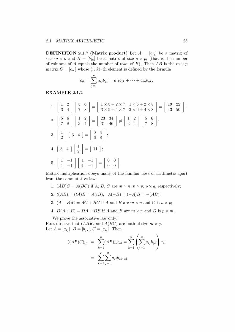
DEFINITION 2.1.7 (Matrix product) Let A = [aij ] be a matrix ofsize m × n and B = [bjk] be a matrix of size n × p; (that is the numberof columns of A equals the number of rows of B). Then AB is the m × pmatrix C = [cik] whose (i, k)–th element is defined by the formula
cik =n
∑
j=1
aijbjk = ai1b1k + · · · + ainbnk.
EXAMPLE 2.1.2
1.
[
1 23 4
] [
5 67 8
]
=
[
1 × 5 + 2 × 7 1 × 6 + 2 × 83 × 5 + 4 × 7 3 × 6 + 4 × 8
]
=
[
19 2243 50
]
;
2.
[
5 67 8
] [
1 23 4
]
=
[
23 3431 46
]
6=[
1 23 4
] [
5 67 8
]
;
3.
[
12
]
[
3 4]
=
[
3 46 8
]
;
4.[
3 4]
[
12
]
=[
11]
;
5.
[
1 −11 −1
] [
1 −11 −1
]
=
[
0 00 0
]
.
Matrix multiplication obeys many of the familiar laws of arithmetic apartfrom the commutative law.
1. (AB)C = A(BC) if A, B, C are m × n, n × p, p × q, respectively;
2. t(AB) = (tA)B = A(tB), A(−B) = (−A)B = −(AB);
3. (A + B)C = AC + BC if A and B are m × n and C is n × p;
4. D(A + B) = DA + DB if A and B are m × n and D is p × m.
We prove the associative law only:First observe that (AB)C and A(BC) are both of size m × q.Let A = [aij ], B = [bjk], C = [ckl]. Then
((AB)C)il =
p∑
k=1
(AB)ikckl =
p∑
k=1
n∑
j=1
aijbjk
ckl
=
p∑
k=1
n∑
j=1
aijbjkckl.
26 CHAPTER 2. MATRICES
Similarly
(A(BC))il =n
∑
j=1
p∑
k=1
aijbjkckl.
However the double summations are equal. For sums of the form
n∑
j=1
p∑
k=1
djk and
p∑
k=1
n∑
j=1
djk
represent the sum of the np elements of the rectangular array [djk], by rowsand by columns, respectively. Consequently
((AB)C)il = (A(BC))il
for 1 ≤ i ≤ m, 1 ≤ l ≤ q. Hence (AB)C = A(BC).
The system of m linear equations in n unknowns
a11x1 + a12x2 + · · · + a1nxn = b1
a21x1 + a22x2 + · · · + a2nxn = b2
...
am1x1 + am2x2 + · · · + amnxn = bm
is equivalent to a single matrix equation
a11 a12 · · · a1n
a21 a22 · · · a2n...
...am1 am2 · · · amn
x1
x2...
xn
=
b1
b2...
bm
,
that is AX = B, where A = [aij ] is the coefficient matrix of the system,
X =
x1
x2...
xn
is the vector of unknowns and B =
b1
b2...
bm
is the vector of
constants.Another useful matrix equation equivalent to the above system of linear
equations is
x1
a11
a21...
am1
+ x2
a12
a22...
am2
+ · · · + xn
a1n
a2n...
amn
=
b1
b2...
bm
.
2.2. LINEAR TRANSFORMATIONS 27
EXAMPLE 2.1.3 The system
x + y + z = 1
x − y + z = 0.
is equivalent to the matrix equation
[
1 1 11 −1 1
]
xyz
=
[
10
]
and to the equation
x
[
11
]
+ y
[
1−1
]
+ z
[
11
]
=
[
10
]
.
2.2 Linear transformations
An n–dimensional column vector is an n × 1 matrix over F . The collectionof all n–dimensional column vectors is denoted by Fn.
Every matrix is associated with an important type of function called alinear transformation.
DEFINITION 2.2.1 (Linear transformation) We can associate withA ∈ Mm×n(F ), the function TA : Fn → Fm, defined by TA(X) = AX for allX ∈ Fn. More explicitly, using components, the above function takes theform
y1 = a11x1 + a12x2 + · · · + a1nxn
y2 = a21x1 + a22x2 + · · · + a2nxn
...
ym = am1x1 + am2x2 + · · · + amnxn,
where y1, y2, · · · , ym are the components of the column vector TA(X).
The function just defined has the property that
TA(sX + tY ) = sTA(X) + tTA(Y ) (2.1)
for all s, t ∈ F and all n–dimensional column vectors X, Y . For
TA(sX + tY ) = A(sX + tY ) = s(AX) + t(AY ) = sTA(X) + tTA(Y ).
28 CHAPTER 2. MATRICES
REMARK 2.2.1 It is easy to prove that if T : Fn → Fm is a functionsatisfying equation 2.1, then T = TA, where A is the m × n matrix whosecolumns are T (E1), . . . , T (En), respectively, where E1, . . . , En are the n–dimensional unit vectors defined by
E1 =
10...0
, . . . , En =
00...1
.
One well–known example of a linear transformation arises from rotatingthe (x, y)–plane in 2-dimensional Euclidean space, anticlockwise through θradians. Here a point (x, y) will be transformed into the point (x1, y1),where
x1 = x cos θ − y sin θ
y1 = x sin θ + y cos θ.
In 3–dimensional Euclidean space, the equations
x1 = x cos θ − y sin θ, y1 = x sin θ + y cos θ, z1 = z;
x1 = x, y1 = y cos φ − z sinφ, z1 = y sinφ + z cos φ;
x1 = x cos ψ − z sinψ, y1 = y, z1 = x sinψ + z cos ψ;
correspond to rotations about the positive z, x and y axes, anticlockwisethrough θ, φ, ψ radians, respectively.
The product of two matrices is related to the product of the correspond-ing linear transformations:
If A is m×n and B is n×p, then the function TATB : F p → Fm, obtainedby first performing TB, then TA is in fact equal to the linear transformationTAB. For if X ∈ F p, we have
TATB(X) = A(BX) = (AB)X = TAB(X).
The following example is useful for producing rotations in 3–dimensionalanimated design. (See [27, pages 97–112].)
EXAMPLE 2.2.1 The linear transformation resulting from successivelyrotating 3–dimensional space about the positive z, x, y–axes, anticlockwisethrough θ, φ, ψ radians respectively, is equal to TABC , where
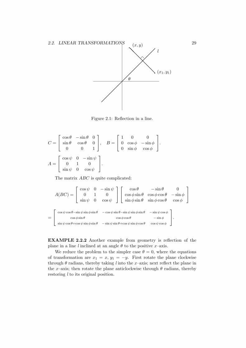
2.2. LINEAR TRANSFORMATIONS 29
θ
l
(x, y)
(x1, y1)
¡¡
¡¡
¡¡
¡¡
¡¡
¡¡
¡
@@
@@
@@
@
Figure 2.1: Reflection in a line.
C =
cos θ − sin θ 0sin θ cos θ 0
0 0 1
, B =
1 0 00 cos φ − sinφ0 sinφ cos φ
.
A =
cos ψ 0 − sinψ0 1 0
sinψ 0 cos ψ
.
The matrix ABC is quite complicated:
A(BC) =
cos ψ 0 − sinψ0 1 0
sin ψ 0 cos ψ
cos θ − sin θ 0cos φ sin θ cos φ cos θ − sinφsin φ sin θ sin φ cos θ cos φ
=
cos ψ cos θ−sin ψ sin φ sin θ − cos ψ sin θ−sin ψ sin φ sin θ − sin ψ cos φ
cos φ sin θ cos φ cos θ − sin φ
sin ψ cos θ+cos ψ sin φ sin θ − sin ψ sin θ+cos ψ sin φ cos θ cos ψ cos φ
.
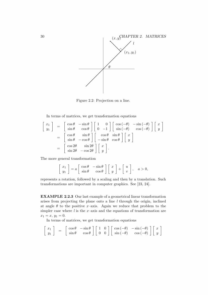
EXAMPLE 2.2.2 Another example from geometry is reflection of theplane in a line l inclined at an angle θ to the positive x–axis.
We reduce the problem to the simpler case θ = 0, where the equationsof transformation are x1 = x, y1 = −y. First rotate the plane clockwisethrough θ radians, thereby taking l into the x–axis; next reflect the plane inthe x–axis; then rotate the plane anticlockwise through θ radians, therebyrestoring l to its original position.
30 CHAPTER 2. MATRICES
θ
l
(x, y)
(x1, y1)
¡¡
¡¡
¡¡
¡¡
¡¡
¡¡
¡
@@
@
Figure 2.2: Projection on a line.
In terms of matrices, we get transformation equations
[
x1
y1
]
=
[
cos θ − sin θsin θ cos θ
] [
1 00 −1
] [
cos (−θ) − sin (−θ)sin (−θ) cos (−θ)
] [
xy
]
=
[
cos θ sin θsin θ − cos θ
] [
cos θ sin θ− sin θ cos θ
] [
xy
]
=
[
cos 2θ sin 2θsin 2θ − cos 2θ
] [
xy
]
.
The more general transformation
[
x1
y1
]
= a
[
cos θ − sin θsin θ cos θ
] [
xy
]
+
[
uv
]
, a > 0,
represents a rotation, followed by a scaling and then by a translation. Suchtransformations are important in computer graphics. See [23, 24].
EXAMPLE 2.2.3 Our last example of a geometrical linear transformationarises from projecting the plane onto a line l through the origin, inclinedat angle θ to the positive x–axis. Again we reduce that problem to thesimpler case where l is the x–axis and the equations of transformation arex1 = x, y1 = 0.
In terms of matrices, we get transformation equations
[
x1
y1
]
=
[
cos θ − sin θsin θ cos θ
] [
1 00 0
] [
cos (−θ) − sin (−θ)sin (−θ) cos (−θ)
] [
xy
]
2.3. RECURRENCE RELATIONS 31
=
[
cos θ 0sin θ 0
] [
cos θ sin θ− sin θ cos θ
] [
xy
]
=
[
cos2 θ cos θ sin θsin θ cos θ sin2 θ
] [
xy
]
.
2.3 Recurrence relations
DEFINITION 2.3.1 (The identity matrix) The n × n matrix In =[δij ], defined by δij = 1 if i = j, δij = 0 if i 6= j, is called the n × n identity
matrix of order n. In other words, the columns of the identity matrix oforder n are the unit vectors E1, · · · , En, respectively.
For example, I2 =
[
1 00 1
]
.
THEOREM 2.3.1 If A is m × n, then ImA = A = AIn.
DEFINITION 2.3.2 (k–th power of a matrix) If A is an n×n matrix,we define Ak recursively as follows: A0 = In and Ak+1 = AkA for k ≥ 0.
For example A1 = A0A = InA = A and hence A2 = A1A = AA.
The usual index laws hold provided AB = BA:
1. AmAn = Am+n, (Am)n = Amn;
2. (AB)n = AnBn;
3. AmBn = BnAm;
4. (A + B)2 = A2 + 2AB + B2;
5. (A + B)n =n
∑
i=0
(
ni
)
AiBn−i;
6. (A + B)(A − B) = A2 − B2.
We now state a basic property of the natural numbers.
AXIOM 2.3.1 (MATHEMATICAL INDUCTION) If Pn denotes a
mathematical statement for each n ≥ 1, satisfying
(i) P1 is true,
32 CHAPTER 2. MATRICES
(ii) the truth of Pn implies that of Pn+1 for each n ≥ 1,
then Pn is true for all n ≥ 1.
EXAMPLE 2.3.1 Let A =
[
7 4−9 −5
]
. Prove that
An =
[
1 + 6n 4n−9n 1 − 6n
]
if n ≥ 1.
Solution. We use the principle of mathematical induction.
Take Pn to be the statement
An =
[
1 + 6n 4n−9n 1 − 6n
]
.
Then P1 asserts that
A1 =
[
1 + 6 × 1 4 × 1−9 × 1 1 − 6 × 1
]
=
[
7 4−9 −5
]
,
which is true. Now let n ≥ 1 and assume that Pn is true. We have to deducethat
An+1 =
[
1 + 6(n + 1) 4(n + 1)−9(n + 1) 1 − 6(n + 1)
]
=
[
7 + 6n 4n + 4−9n − 9 −5 − 6n
]
.
Now
An+1 = AnA
=
[
1 + 6n 4n−9n 1 − 6n
] [
7 4−9 −5
]
=
[
(1 + 6n)7 + (4n)(−9) (1 + 6n)4 + (4n)(−5)(−9n)7 + (1 − 6n)(−9) (−9n)4 + (1 − 6n)(−5)
]
=
[
7 + 6n 4n + 4−9n − 9 −5 − 6n
]
,
and “the induction goes through”.
The last example has an application to the solution of a system of re-
currence relations:
2.4. PROBLEMS 33
EXAMPLE 2.3.2 The following system of recurrence relations holds forall n ≥ 0:
xn+1 = 7xn + 4yn
yn+1 = −9xn − 5yn.
Solve the system for xn and yn in terms of x0 and y0.
Solution. Combine the above equations into a single matrix equation[
xn+1
yn+1
]
=
[
7 4−9 −5
] [
xn
yn
]
,
or Xn+1 = AXn, where A =
[
7 4−9 −5
]
and Xn =
[
xn
yn
]
.
We see that
X1 = AX0
X2 = AX1 = A(AX0) = A2X0
...
Xn = AnX0.
(The truth of the equation Xn = AnX0 for n ≥ 1, strictly speakingfollows by mathematical induction; however for simple cases such as theabove, it is customary to omit the strict proof and supply instead a fewlines of motivation for the inductive statement.)
Hence the previous example gives[
xn
yn
]
= Xn =
[
1 + 6n 4n−9n 1 − 6n
] [
x0
y0
]
=
[
(1 + 6n)x0 + (4n)y0
(−9n)x0 + (1 − 6n)y0
]
,
and hence xn = (1+6n)x0 +4ny0 and yn = (−9n)x0 +(1−6n)y0, for n ≥ 1.
2.4 PROBLEMS
1. Let A, B, C, D be matrices defined by
A =
3 0−1 2
1 1
, B =
1 5 2−1 1 0−4 1 3
,
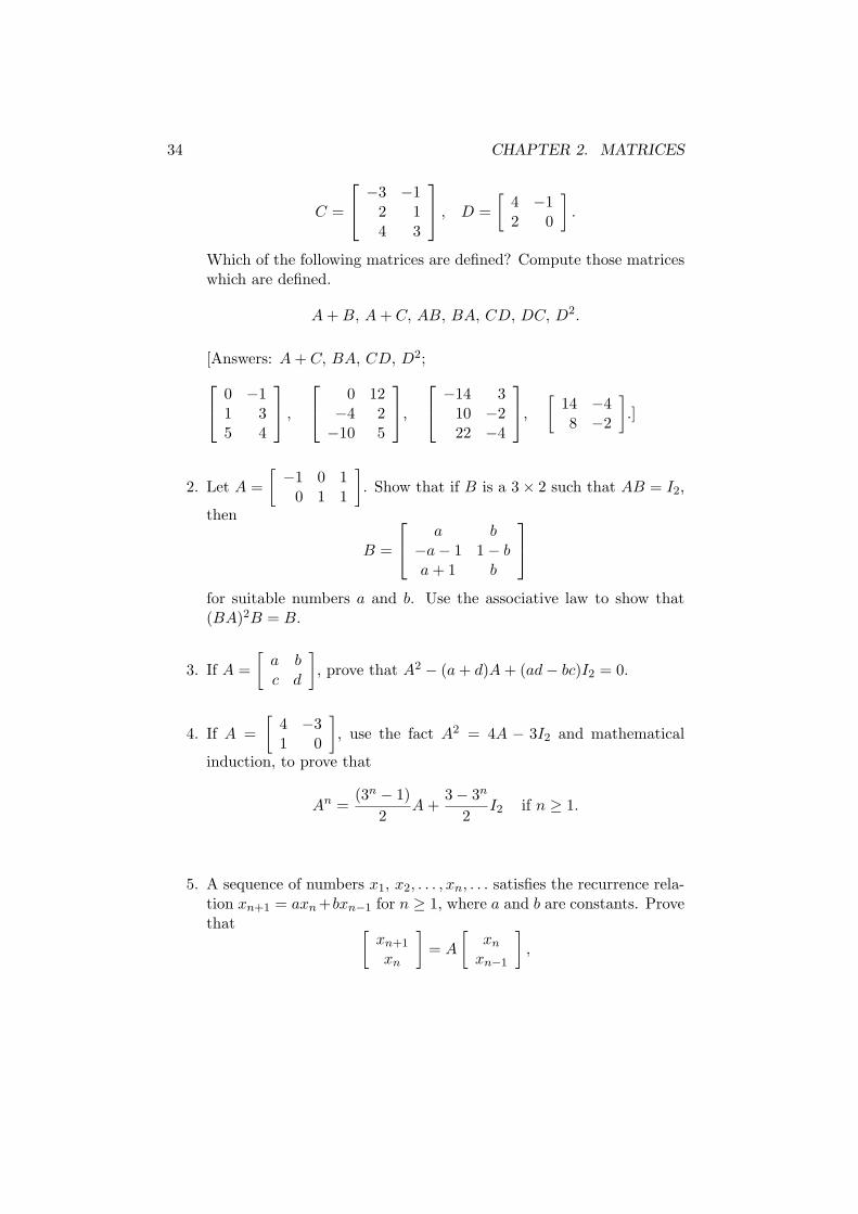
34 CHAPTER 2. MATRICES
C =
−3 −12 14 3
, D =
[
4 −12 0
]
.
Which of the following matrices are defined? Compute those matriceswhich are defined.
A + B, A + C, AB, BA, CD, DC, D2.
[Answers: A + C, BA, CD, D2;
0 −11 35 4
,
0 12−4 2−10 5
,
−14 310 −222 −4
,
[
14 −48 −2
]
.]
2. Let A =
[
−1 0 10 1 1
]
. Show that if B is a 3 × 2 such that AB = I2,
then
B =
a b−a − 1 1 − ba + 1 b
for suitable numbers a and b. Use the associative law to show that(BA)2B = B.
3. If A =
[
a bc d
]
, prove that A2 − (a + d)A + (ad − bc)I2 = 0.
4. If A =
[
4 −31 0
]
, use the fact A2 = 4A − 3I2 and mathematical
induction, to prove that
An =(3n − 1)
2A +
3 − 3n
2I2 if n ≥ 1.
5. A sequence of numbers x1, x2, . . . , xn, . . . satisfies the recurrence rela-tion xn+1 = axn +bxn−1 for n ≥ 1, where a and b are constants. Provethat
[
xn+1
xn
]
= A
[
xn
xn−1
]
,
2.4. PROBLEMS 35
where A =
[
a b1 0
]
and hence express
[
xn+1
xn
]
in terms of
[
x1
x0
]
.
If a = 4 and b = −3, use the previous question to find a formula forxn in terms of x1 and x0.
[Answer:
xn =3n − 1
2x1 +
3 − 3n
2x0.]
6. Let A =
[
2a −a2
1 0
]
.
(a) Prove that
An =
[
(n + 1)an −nan+1
nan−1 (1 − n)an
]
if n ≥ 1.
(b) A sequence x0, x1, . . . , xn, . . . satisfies xn+1 = 2axn − a2xn−1 forn ≥ 1. Use part (a) and the previous question to prove thatxn = nan−1x1 + (1 − n)anx0 for n ≥ 1.
7. Let A =
[
a bc d
]
and suppose that λ1 and λ2 are the roots of the
quadratic polynomial x2−(a+d)x+ad−bc. (λ1 and λ2 may be equal.)
Let kn be defined by k0 = 0, k1 = 1 and for n ≥ 2
kn =
n∑
i=1
λn−i1 λi−1
2 .
Prove thatkn+1 = (λ1 + λ2)kn − λ1λ2kn−1,
if n ≥ 1. Also prove that
kn =
{
(λn1 − λn
2 )/(λ1 − λ2) if λ1 6= λ2,
nλn−11 if λ1 = λ2.
Use mathematical induction to prove that if n ≥ 1,
An = knA − λ1λ2kn−1I2,
[Hint: Use the equation A2 = (a + d)A − (ad − bc)I2.]
36 CHAPTER 2. MATRICES
8. Use Question 7 to prove that if A =
[
1 22 1
]
, then
An =3n
2
[
1 11 1
]
+(−1)n−1
2
[
−1 11 −1
]
if n ≥ 1.
9. The Fibonacci numbers are defined by the equations F0 = 0, F1 = 1and Fn+1 = Fn + Fn−1 if n ≥ 1. Prove that
Fn =1√5
((
1 +√
5
2
)n
−(
1 −√
5
2
)n)
if n ≥ 0.
10. Let r > 1 be an integer. Let a and b be arbitrary positive integers.Sequences xn and yn of positive integers are defined in terms of a andb by the recurrence relations
xn+1 = xn + ryn
yn+1 = xn + yn,
for n ≥ 0, where x0 = a and y0 = b.
Use Question 7 to prove that
xn
yn→ √
r as n → ∞.
2.5 Non–singular matrices
DEFINITION 2.5.1 (Non–singular matrix) A matrix A ∈ Mn×n(F )is called non–singular or invertible if there exists a matrix B ∈ Mn×n(F )such that
AB = In = BA.
Any matrix B with the above property is called an inverse of A. If A doesnot have an inverse, A is called singular.
THEOREM 2.5.1 (Inverses are unique) If A has inverses B and C,then B = C.
2.5. NON–SINGULAR MATRICES 37
Proof. Let B and C be inverses of A. Then AB = In = BA and AC =In = CA. Then B(AC) = BIn = B and (BA)C = InC = C. Hence becauseB(AC) = (BA)C, we deduce that B = C.
REMARK 2.5.1 If A has an inverse, it is denoted by A−1. So
AA−1 = In = A−1A.
Also if A is non–singular, it follows that A−1 is also non–singular and
(A−1)−1 = A.
THEOREM 2.5.2 If A and B are non–singular matrices of the same size,then so is AB. Moreover
(AB)−1 = B−1A−1.
Proof.
(AB)(B−1A−1) = A(BB−1)A−1 = AInA−1 = AA−1 = In.
Similarly(B−1A−1)(AB) = In.
REMARK 2.5.2 The above result generalizes to a product of m non–singular matrices: If A1, . . . , Am are non–singular n × n matrices, then theproduct A1 . . . Am is also non–singular. Moreover
(A1 . . . Am)−1 = A−1m . . . A−1
1 .
(Thus the inverse of the product equals the product of the inverses in the
reverse order.)
EXAMPLE 2.5.1 If A and B are n × n matrices satisfying A2 = B2 =(AB)2 = In, prove that AB = BA.
Solution. Assume A2 = B2 = (AB)2 = In. Then A, B, AB are non–singular and A−1 = A, B−1 = B, (AB)−1 = AB.
But (AB)−1 = B−1A−1 and hence AB = BA.
EXAMPLE 2.5.2 A =
[
1 24 8
]
is singular. For suppose B =
[
a bc d
]
is an inverse of A. Then the equation AB = I2 gives[
1 24 8
] [
a bc d
]
=
[
1 00 1
]
38 CHAPTER 2. MATRICES
and equating the corresponding elements of column 1 of both sides gives thesystem
a + 2c = 1
4a + 8c = 0
which is clearly inconsistent.
THEOREM 2.5.3 Let A =
[
a bc d
]
and ∆ = ad − bc 6= 0. Then A is
non–singular. Also
A−1 = ∆−1
[
d −b−c a
]
.
REMARK 2.5.3 The expression ad − bc is called the determinant of A
and is denoted by the symbols detA or
∣
∣
∣
∣
a bc d
∣
∣
∣
∣
.
Proof. Verify that the matrix B = ∆−1
[
d −b−c a
]
satisfies the equation
AB = I2 = BA.
EXAMPLE 2.5.3 Let
A =
0 1 00 0 15 0 0
.
Verify that A3 = 5I3, deduce that A is non–singular and find A−1.
Solution. After verifying that A3 = 5I3, we notice that
A
(
1
5A2
)
= I3 =
(
1
5A2
)
A.
Hence A is non–singular and A−1 = 15A2.
THEOREM 2.5.4 If the coefficient matrix A of a system of n equationsin n unknowns is non–singular, then the system AX = B has the uniquesolution X = A−1B.
Proof. Assume that A−1 exists.
2.5. NON–SINGULAR MATRICES 39
1. (Uniqueness.) Assume that AX = B. Then
(A−1A)X = A−1B,
InX = A−1B,
X = A−1B.
2. (Existence.) Let X = A−1B. Then
AX = A(A−1B) = (AA−1)B = InB = B.
THEOREM 2.5.5 (Cramer’s rule for 2 equations in 2 unknowns)The system
ax + by = e
cx + dy = f
has a unique solution if ∆ =
∣
∣
∣
∣
a bc d
∣
∣
∣
∣
6= 0, namely
x =∆1
∆, y =
∆2
∆,
where
∆1 =
∣
∣
∣
∣
e bf d
∣
∣
∣
∣
and ∆2 =
∣
∣
∣
∣
a ec f
∣
∣
∣
∣
.
Proof. Suppose ∆ 6= 0. Then A =
[
a bc d
]
has inverse
A−1 = ∆−1
[
d −b−c a
]
and we know that the system
A
[
xy
]
=
[
ef
]
has the unique solution[
xy
]
= A−1
[
ef
]
=1
∆
[
d −b−c a
] [
ef
]
=1
∆
[
de − bf−ce + af
]
=1
∆
[
∆1
∆2
]
=
[
∆1/∆∆2/∆
]
.
Hence x = ∆1/∆, y = ∆2/∆.
40 CHAPTER 2. MATRICES
COROLLARY 2.5.1 The homogeneous system
ax + by = 0
cx + dy = 0
has only the trivial solution if ∆ =
∣
∣
∣
∣
a bc d
∣
∣
∣
∣
6= 0.
EXAMPLE 2.5.4 The system
7x + 8y = 100
2x − 9y = 10
has the unique solution x = ∆1/∆, y = ∆2/∆, where
∆=
˛
˛
˛
˛
˛
˛
7 82 −9
˛
˛
˛
˛
˛
˛
=−79, ∆1=
˛
˛
˛
˛
˛
˛
100 810 −9
˛
˛
˛
˛
˛
˛
=−980, ∆2=
˛
˛
˛
˛
˛
˛
7 1002 10
˛
˛
˛
˛
˛
˛
=−130.
So x = 98079 and y = 130
79 .
THEOREM 2.5.6 Let A be a square matrix. If A is non–singular, thehomogeneous system AX = 0 has only the trivial solution. Equivalently,if the homogenous system AX = 0 has a non–trivial solution, then A issingular.
Proof. If A is non–singular and AX = 0, then X = A−10 = 0.
REMARK 2.5.4 If A∗1, . . . , A∗n denote the columns of A, then the equa-tion
AX = x1A∗1 + . . . + xnA∗n
holds. Consequently theorem 2.5.6 tells us that if there exist x1, . . . , xn, not
all zero, such that
x1A∗1 + . . . + xnA∗n = 0,
that is, if the columns of A are linearly dependent, then A is singular. Anequivalent way of saying that the columns of A are linearly dependent is thatone of the columns of A is expressible as a sum of certain scalar multiplesof the remaining columns of A; that is one column is a linear combination
of the remaining columns.
2.5. NON–SINGULAR MATRICES 41
EXAMPLE 2.5.5
A =
1 2 31 0 13 4 7
is singular. For it can be verified that A has reduced row–echelon form
1 0 10 1 10 0 0
and consequently AX = 0 has a non–trivial solution x = −1, y = −1, z = 1.
REMARK 2.5.5 More generally, if A is row–equivalent to a matrix con-taining a zero row, then A is singular. For then the homogeneous systemAX = 0 has a non–trivial solution.
An important class of non–singular matrices is that of the elementary
row matrices.
DEFINITION 2.5.2 (Elementary row matrices) To each of the threetypes of elementary row operation, there corresponds an elementary row
matrix, denoted by Eij , Ei(t), Eij(t):
1. Eij , (i 6= j) is obtained from the identity matrix In by interchangingrows i and j.
2. Ei(t), (t 6= 0) is obtained by multiplying the i–th row of In by t.
3. Eij(t), (i 6= j) is obtained from In by adding t times the j–th row ofIn to the i–th row.
EXAMPLE 2.5.6 (n = 3.)
E23 =
1 0 00 0 10 1 0
, E2(−1) =
1 0 00 −1 00 0 1
, E23(−1) =
1 0 00 1 −10 0 1
.
The elementary row matrices have the following distinguishing property:
THEOREM 2.5.7 If a matrix A is pre–multiplied by an elementary rowmatrix, the resulting matrix is the one obtained by performing the corre-sponding elementary row–operation on A.
42 CHAPTER 2. MATRICES
EXAMPLE 2.5.7
E23
a bc de f
=
1 0 00 0 10 1 0
a bc de f
=
a be fc d
.
COROLLARY 2.5.2 Elementary row–matrices are non–singular. Indeed
1. E−1ij = Eij ;
2. E−1i (t) = Ei(t
−1);
3. (Eij(t))−1 = Eij(−t).
Proof. Taking A = In in the above theorem, we deduce the followingequations:
EijEij = In
Ei(t)Ei(t−1) = In = Ei(t
−1)Ei(t) if t 6= 0
Eij(t)Eij(−t) = In = Eij(−t)Eij(t).
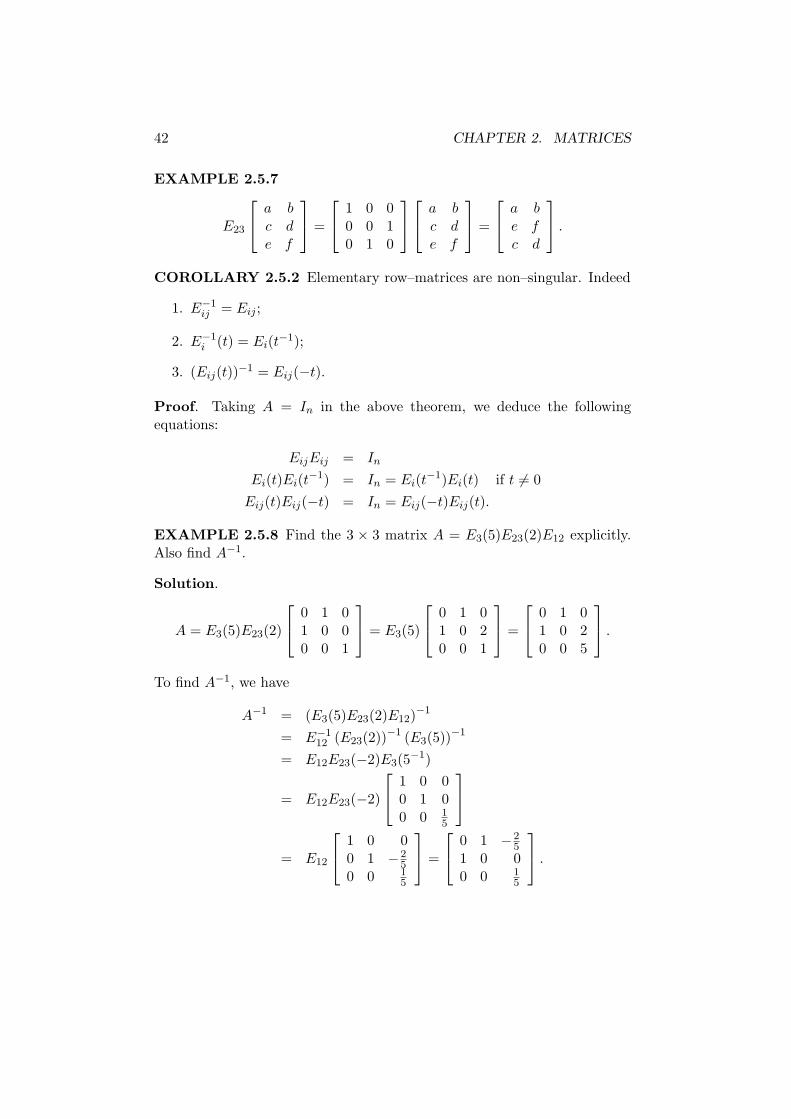
EXAMPLE 2.5.8 Find the 3 × 3 matrix A = E3(5)E23(2)E12 explicitly.Also find A−1.
Solution.
A = E3(5)E23(2)
0 1 01 0 00 0 1
= E3(5)
0 1 01 0 20 0 1
=
0 1 01 0 20 0 5
.
To find A−1, we have
A−1 = (E3(5)E23(2)E12)−1
= E−112 (E23(2))−1 (E3(5))−1
= E12E23(−2)E3(5−1)
= E12E23(−2)
1 0 00 1 00 0 1
5
= E12
1 0 00 1 −2
50 0 1
5
=
0 1 −25
1 0 00 0 1
5
.
2.5. NON–SINGULAR MATRICES 43
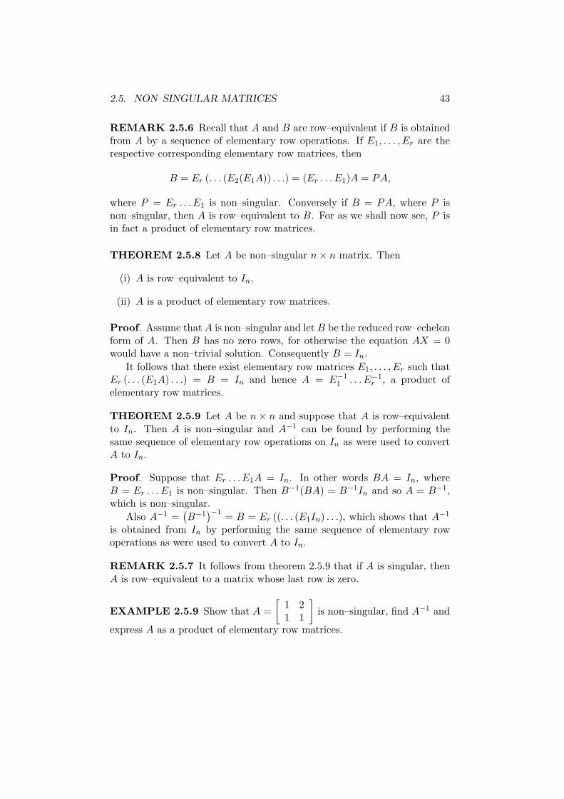
REMARK 2.5.6 Recall that A and B are row–equivalent if B is obtainedfrom A by a sequence of elementary row operations. If E1, . . . , Er are therespective corresponding elementary row matrices, then
B = Er (. . . (E2(E1A)) . . .) = (Er . . . E1)A = PA,
where P = Er . . . E1 is non–singular. Conversely if B = PA, where P isnon–singular, then A is row–equivalent to B. For as we shall now see, P isin fact a product of elementary row matrices.
THEOREM 2.5.8 Let A be non–singular n × n matrix. Then
(i) A is row–equivalent to In,
(ii) A is a product of elementary row matrices.
Proof. Assume that A is non–singular and let B be the reduced row–echelonform of A. Then B has no zero rows, for otherwise the equation AX = 0would have a non–trivial solution. Consequently B = In.
It follows that there exist elementary row matrices E1, . . . , Er such thatEr (. . . (E1A) . . .) = B = In and hence A = E−1
1 . . . E−1r , a product of
elementary row matrices.
THEOREM 2.5.9 Let A be n × n and suppose that A is row–equivalentto In. Then A is non–singular and A−1 can be found by performing thesame sequence of elementary row operations on In as were used to convertA to In.
Proof. Suppose that Er . . . E1A = In. In other words BA = In, whereB = Er . . . E1 is non–singular. Then B−1(BA) = B−1In and so A = B−1,which is non–singular.
Also A−1 =(
B−1)−1
= B = Er ((. . . (E1In) . . .), which shows that A−1
is obtained from In by performing the same sequence of elementary rowoperations as were used to convert A to In.
REMARK 2.5.7 It follows from theorem 2.5.9 that if A is singular, thenA is row–equivalent to a matrix whose last row is zero.
EXAMPLE 2.5.9 Show that A =
[
1 21 1
]
is non–singular, find A−1 and
express A as a product of elementary row matrices.
44 CHAPTER 2. MATRICES
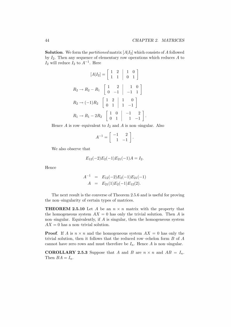
Solution. We form the partitioned matrix [A|I2] which consists of A followedby I2. Then any sequence of elementary row operations which reduces A toI2 will reduce I2 to A−1. Here
[A|I2] =
[
1 2 1 01 1 0 1
]
R2 → R2 − R1
[
1 2 1 00 −1 −1 1
]
R2 → (−1)R2
[
1 2 1 00 1 1 −1
]
R1 → R1 − 2R2
[
1 0 −1 20 1 1 −1
]
.
Hence A is row–equivalent to I2 and A is non–singular. Also
A−1 =
[
−1 21 −1
]
.
We also observe that
E12(−2)E2(−1)E21(−1)A = I2.
Hence
A−1 = E12(−2)E2(−1)E21(−1)
A = E21(1)E2(−1)E12(2).
The next result is the converse of Theorem 2.5.6 and is useful for provingthe non–singularity of certain types of matrices.
THEOREM 2.5.10 Let A be an n × n matrix with the property thatthe homogeneous system AX = 0 has only the trivial solution. Then A isnon–singular. Equivalently, if A is singular, then the homogeneous systemAX = 0 has a non–trivial solution.
Proof. If A is n × n and the homogeneous system AX = 0 has only thetrivial solution, then it follows that the reduced row–echelon form B of Acannot have zero rows and must therefore be In. Hence A is non–singular.
COROLLARY 2.5.3 Suppose that A and B are n × n and AB = In.Then BA = In.
2.5. NON–SINGULAR MATRICES 45
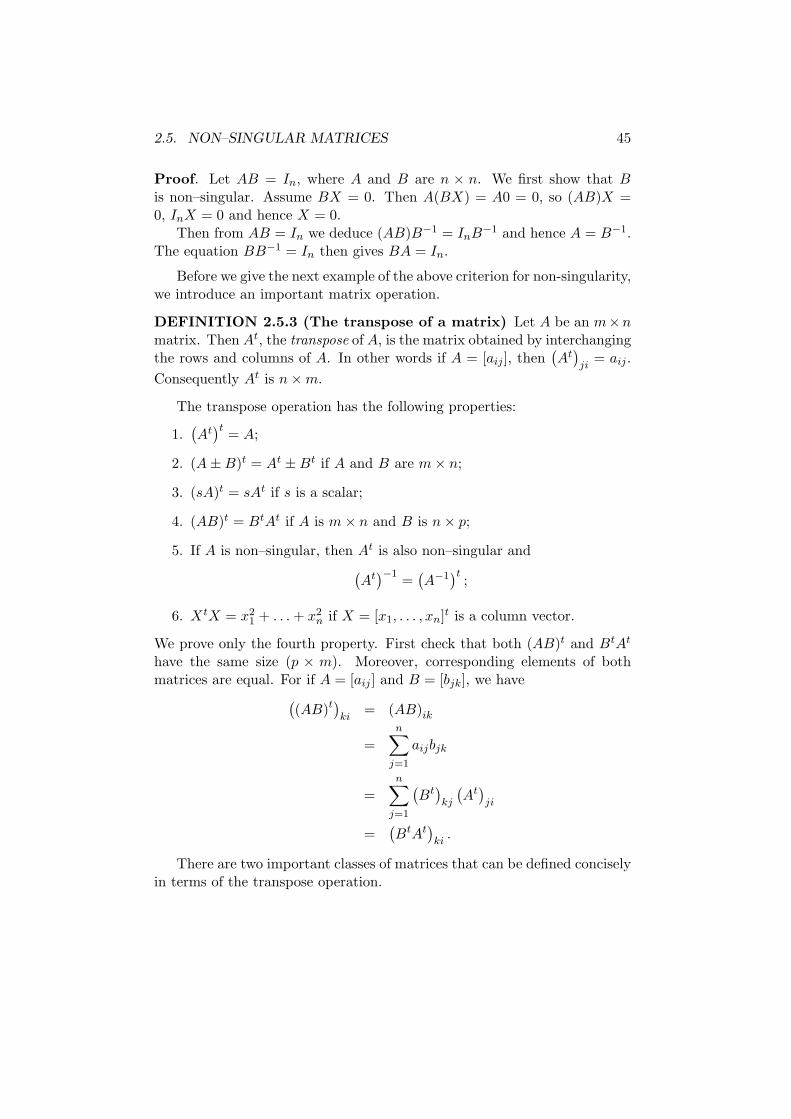
Proof. Let AB = In, where A and B are n × n. We first show that Bis non–singular. Assume BX = 0. Then A(BX) = A0 = 0, so (AB)X =0, InX = 0 and hence X = 0.
Then from AB = In we deduce (AB)B−1 = InB−1 and hence A = B−1.The equation BB−1 = In then gives BA = In.
Before we give the next example of the above criterion for non-singularity,we introduce an important matrix operation.
DEFINITION 2.5.3 (The transpose of a matrix) Let A be an m×nmatrix. Then At, the transpose of A, is the matrix obtained by interchangingthe rows and columns of A. In other words if A = [aij ], then
(
At)
ji= aij .
Consequently At is n × m.
The transpose operation has the following properties:
1.(
At)t
= A;
2. (A ± B)t = At ± Bt if A and B are m × n;
3. (sA)t = sAt if s is a scalar;
4. (AB)t = BtAt if A is m × n and B is n × p;
5. If A is non–singular, then At is also non–singular and
(
At)−1
=(
A−1)t
;
6. XtX = x21 + . . . + x2
n if X = [x1, . . . , xn]t is a column vector.
We prove only the fourth property. First check that both (AB)t and BtAt
have the same size (p × m). Moreover, corresponding elements of bothmatrices are equal. For if A = [aij ] and B = [bjk], we have
(
(AB)t)
ki= (AB)ik
=n
∑
j=1
aijbjk
=n
∑
j=1
(
Bt)
kj
(
At)
ji
=(
BtAt)
ki.
There are two important classes of matrices that can be defined conciselyin terms of the transpose operation.
46 CHAPTER 2. MATRICES
DEFINITION 2.5.4 (Symmetric matrix) A matrix A is symmetric ifAt = A. In other words A is square (n × n say) and aji = aij for all1 ≤ i ≤ n, 1 ≤ j ≤ n. Hence
A =
[
a bb c
]
is a general 2 × 2 symmetric matrix.
DEFINITION 2.5.5 (Skew–symmetric matrix) A matrix A is calledskew–symmetric if At = −A. In other words A is square (n × n say) andaji = −aij for all 1 ≤ i ≤ n, 1 ≤ j ≤ n.
REMARK 2.5.8 Taking i = j in the definition of skew–symmetric matrixgives aii = −aii and so aii = 0. Hence
A =
[
0 b−b 0
]
is a general 2 × 2 skew–symmetric matrix.
We can now state a second application of the above criterion for non–singularity.
COROLLARY 2.5.4 Let B be an n × n skew–symmetric matrix. ThenA = In − B is non–singular.
Proof. Let A = In − B, where Bt = −B. By Theorem 2.5.10 it suffices toshow that AX = 0 implies X = 0.
We have (In − B)X = 0, so X = BX. Hence XtX = XtBX.
Taking transposes of both sides gives
(XtBX)t = (XtX)t
XtBt(Xt)t = Xt(Xt)t
Xt(−B)X = XtX
−XtBX = XtX = XtBX.
Hence XtX = −XtX and XtX = 0. But if X = [x1, . . . , xn]t, then XtX =x2
1 + . . . + x2n = 0 and hence x1 = 0, . . . , xn = 0.
2.6. LEAST SQUARES SOLUTION OF EQUATIONS 47
2.6 Least squares solution of equations
Suppose AX = B represents a system of linear equations with real coeffi-cients which may be inconsistent, because of the possibility of experimentalerrors in determining A or B. For example, the system
x = 1
y = 2
x + y = 3.001
is inconsistent.It can be proved that the associated system AtAX = AtB is always
consistent and that any solution of this system minimizes the sum r21 + . . .+
r2m, where r1, . . . , rm (the residuals) are defined by
ri = ai1x1 + . . . + ainxn − bi,
for i = 1, . . . , m. The equations represented by AtAX = AtB are called thenormal equations corresponding to the system AX = B and any solutionof the system of normal equations is called a least squares solution of theoriginal system.
EXAMPLE 2.6.1 Find a least squares solution of the above inconsistentsystem.
Solution. Here A =
1 00 11 1
, X =
[
xy
]
, B =
12
3.001
.
Then AtA =
[
1 0 10 1 1
]
1 00 11 1
=
[
2 11 2
]
.
Also AtB =
[
1 0 10 1 1
]
12
3.001
=
[
4.0015.001
]
.
So the normal equations are
2x + y = 4.001
x + 2y = 5.001
which have the unique solution
x =3.001
3, y =
6.001
3.
48 CHAPTER 2. MATRICES
EXAMPLE 2.6.2 Points (x1, y1), . . . , (xn, yn) are experimentally deter-mined and should lie on a line y = mx + c. Find a least squares solution tothe problem.
Solution. The points have to satisfy
mx1 + c = y1
...
mxn + c = yn,
or Ax = B, where
A =
x1 1...
...xn 1
, X =
[
mc
]
, B =
y1...
yn
.
The normal equations are given by (AtA)X = AtB. Here
AtA =
[
x1 . . . xn
1 . . . 1
]
x1 1...
...xn 1
=
[
x21 + . . . + x2
n x1 + . . . + xn
x1 + . . . + xn n
]
Also
AtB =
[
x1 . . . xn
1 . . . 1
]
y1...
yn
=
[
x1y1 + . . . + xnyn
y1 + . . . + yn
]
.
It is not difficult to prove that
∆ = det (AtA) =∑
1≤i<j≤n
(xi − xj)2,
which is positive unless x1 = . . . = xn. Hence if not all of x1, . . . , xn areequal, AtA is non–singular and the normal equations have a unique solution.This can be shown to be
m =1
∆
∑
1≤i<j≤n
(xi − xj)(yi − yj), c =1
∆
∑
1≤i<j≤n
(xiyj − xjyi)(xi − xj).
REMARK 2.6.1 The matrix AtA is symmetric.
2.7. PROBLEMS 49
2.7 PROBLEMS
1. Let A =
[
1 4−3 1
]
. Prove that A is non–singular, find A−1 and
express A as a product of elementary row matrices.
[Answer: A−1 =
[
113 − 4
13313
113
]
,
A = E21(−3)E2(13)E12(4) is one such decomposition.]
2. A square matrix D = [dij ] is called diagonal if dij = 0 for i 6= j. (Thatis the off–diagonal elements are zero.) Prove that pre–multiplicationof a matrix A by a diagonal matrix D results in matrix DA whoserows are the rows of A multiplied by the respective diagonal elementsof D. State and prove a similar result for post–multiplication by adiagonal matrix.
Let diag (a1, . . . , an) denote the diagonal matrix whose diagonal ele-ments dii are a1, . . . , an, respectively. Show that
diag (a1, . . . , an)diag (b1, . . . , bn) = diag (a1b1, . . . , anbn)
and deduce that if a1 . . . an 6= 0, then diag (a1, . . . , an) is non–singularand
(diag (a1, . . . , an))−1 = diag (a−11 , . . . , a−1
n ).
Also prove that diag (a1, . . . , an) is singular if ai = 0 for some i.
3. Let A =
0 0 21 2 63 7 9
. Prove that A is non–singular, find A−1 and
express A as a product of elementary row matrices.
[Answers: A−1 =
−12 7 −292 −3 112 0 0
,
A = E12E31(3)E23E3(2)E12(2)E13(24)E23(−9) is one such decompo-sition.]
50 CHAPTER 2. MATRICES
4. Find the rational number k for which the matrix A =
1 2 k3 −1 15 3 −5
is singular. [Answer: k = −3.]
5. Prove that A =
[
1 2−2 −4
]
is singular and find a non–singular matrix
P such that PA has last row zero.
6. If A =
[
1 4−3 1
]
, verify that A2 − 2A + 13I2 = 0 and deduce that
A−1 = − 113(A − 2I2).
7. Let A =
1 1 −10 0 12 1 2
.
(i) Verify that A3 = 3A2 − 3A + I3.
(ii) Express A4 in terms of A2, A and I3 and hence calculate A4
explicitly.
(iii) Use (i) to prove that A is non–singular and find A−1 explicitly.
[Answers: (ii) A4 = 6A2 − 8A + 3I3 =
−11 −8 −412 9 420 16 5
;
(iii) A−1 = A2 − 3A + 3I3 =
−1 −3 12 4 −10 1 0
.]
8. (i) Let B be an n×n matrix such that B3 = 0. If A = In−B, provethat A is non–singular and A−1 = In + B + B2.
Show that the system of linear equations AX = b has the solution
X = b + Bb + B2b.
(ii) If B =
0 r s0 0 t0 0 0
, verify that B3 = 0 and use (i) to determine
(I3 − B)−1 explicitly.
2.7. PROBLEMS 51
[Answer:
1 r s + rt0 1 t0 0 1
.]
9. Let A be n × n.
(i) If A2 = 0, prove that A is singular.
(ii) If A2 = A and A 6= In, prove that A is singular.
10. Use Question 7 to solve the system of equations
x + y − z = a
z = b
2x + y + 2z = c
where a, b, c are given rationals. Check your answer using the Gauss–Jordan algorithm.
[Answer: x = −a − 3b + c, y = 2a + 4b − c, z = b.]
11. Determine explicitly the following products of 3 × 3 elementary rowmatrices.
(i) E12E23 (ii) E1(5)E12 (iii) E12(3)E21(−3) (iv) (E1(100))−1
(v) E−112 (vi) (E12(7))−1 (vii) (E12(7)E31(1))−1.
[Answers: (i)
2
4
0 0 11 0 00 1 0
3
5 (ii)
2
4
0 5 01 0 00 0 1
3
5 (iii)
2
4
−8 3 0−3 1 0
0 0 1
3
5
(iv)
2
4
1/100 0 00 1 00 0 1
3
5 (v)
2
4
0 1 01 0 00 0 1
3
5 (vi)
2
4
1 −7 00 1 00 0 1
3
5 (vii)
2
4
1 −7 00 1 0
−1 7 1
3
5.]
12. Let A be the following product of 4 × 4 elementary row matrices:
A = E3(2)E14E42(3).
Find A and A−1 explicitly.
[Answers: A =
2
6
6
4
0 3 0 10 1 0 00 0 2 01 0 0 0
3
7
7
5
, A−1 =
2
6
6
4
0 0 0 10 1 0 00 0 1/2 01 −3 0 0
3
7
7
5
.]
52 CHAPTER 2. MATRICES
13. Determine which of the following matrices over Z2 are non–singularand find the inverse, where possible.
(a)
2
6
6
4
1 1 0 10 0 1 11 1 1 11 0 0 1
3
7
7
5
(b)
2
6
6
4
1 1 0 10 1 1 11 0 1 01 1 0 1
3
7
7
5
. [Answer: (a)
2
6
6
4
1 1 1 11 0 0 11 0 1 01 1 1 0
3
7
7
5
.]
14. Determine which of the following matrices are non–singular and findthe inverse, where possible.
(a)
2
4
1 1 1−1 1 0
2 0 0
3
5 (b)
2
4
2 2 41 0 10 1 0
3
5 (c)
2
4
4 6 −30 0 70 0 5
3
5
(d)
2
4
2 0 00 −5 00 0 7
3
5 (e)
2
6
6
4
1 2 4 60 1 2 00 0 1 20 0 0 2
3
7
7
5
(f)
2
4
1 2 34 5 65 7 9
3
5.
[Answers: (a)
2
4
0 0 1/20 1 1/21 −1 −1
3
5 (b)
2
4
−1/2 2 10 0 1
1/2 −1 −1
3
5 (d)
2
4
1/2 0 00 −1/5 00 0 1/7
3
5
(e)
2
6
6
4
1 −2 0 −30 1 −2 20 0 1 −10 0 0 1/2
3
7
7
5
.]
15. Let A be a non–singular n × n matrix. Prove that At is non–singularand that (At)−1 = (A−1)t.
16. Prove that A =
[
a bc d
]
has no inverse if ad − bc = 0.
[Hint: Use the equation A2 − (a + d)A + (ad − bc)I2 = 0.]
17. Prove that the real matrix A =
2
4
1 a b−a 1 c−b −c 1
3
5 is non–singular by prov-
ing that A is row–equivalent to I3.
18. If P−1AP = B, prove that P−1AnP = Bn for n ≥ 1.
2.7. PROBLEMS 53
19. Let A =
[
2/3 1/41/3 3/4
]
, P =
[
1 3−1 4
]
. Verify that P−1AP =[
5/12 00 1
]
and deduce that
An =1
7
[
3 34 4
]
+1
7
(
5
12
)n [
4 −3−4 3
]
.
20. Let A =
[
a bc d
]
be a Markov matrix; that is a matrix whose elements
are non–negative and satisfy a+c = 1 = b+d. Also let P =
[
b 1c −1
]
.
Prove that if A 6= I2 then
(i) P is non–singular and P−1AP =
[
1 00 a + d − 1
]
,
(ii) An → 1
b + c
[
b bc c
]
as n → ∞, if A 6=[
0 11 0
]
.
21. If X =
1 23 45 6
and Y =
−134
, find XXt, XtX, Y Y t, Y tY .
[Answers:
5 11 1711 25 3917 39 61
,
[
35 4444 56
]
,
1 −3 −4−3 9 12−4 12 16
, 26.]
22. Prove that the system of linear equations
x + 2y = 4x + y = 5
3x + 5y = 12
is inconsistent and find a least squares solution of the system.
[Answer: x = 6, y = −7/6.]
23. The points (0, 0), (1, 0), (2, −1), (3, 4), (4, 8) are required to lie on aparabola y = a + bx + cx2. Find a least squares solution for a, b, c.Also prove that no parabola passes through these points.
[Answer: a = 15 , b = −2, c = 1.]
54 CHAPTER 2. MATRICES
24. If A is a symmetric n×n real matrix and B is n×m, prove that BtABis a symmetric m × m matrix.
25. If A is m × n and B is n × m, prove that AB is singular if m > n.
26. Let A and B be n × n. If A or B is singular, prove that AB is alsosingular.
Chapter 3
SUBSPACES
3.1 Introduction
Throughout this chapter, we will be studying Fn, the set of n–dimensionalcolumn vectors with components from a field F . We continue our studyof matrices by considering an important class of subsets of Fn called sub-
spaces. These arise naturally for example, when we solve a system of mlinear homogeneous equations in n unknowns.
We also study the concept of linear dependence of a family of vectors.This was introduced briefly in Chapter 2, Remark 2.5.4. Other topics dis-cussed are the row space, column space and null space of a matrix over F ,the dimension of a subspace, particular examples of the latter being the rank
and nullity of a matrix.
3.2 Subspaces of Fn
DEFINITION 3.2.1 A subset S of Fn is called a subspace of Fn if
1. The zero vector belongs to S; (that is, 0 ∈ S);
2. If u ∈ S and v ∈ S, then u + v ∈ S; (S is said to be closed undervector addition);
3. If u ∈ S and t ∈ F , then tu ∈ S; (S is said to be closed under scalarmultiplication).
EXAMPLE 3.2.1 Let A ∈ Mm×n(F ). Then the set of vectors X ∈ Fn
satisfying AX = 0 is a subspace of Fn called the null space of A and isdenoted here by N(A). (It is sometimes called the solution space of A.)
55
56 CHAPTER 3. SUBSPACES
Proof. (1) A0 = 0, so 0 ∈ N(A); (2) If X, Y ∈ N(A), then AX = 0 andAY = 0, so A(X + Y ) = AX + AY = 0 + 0 = 0 and so X + Y ∈ N(A); (3)If X ∈ N(A) and t ∈ F , then A(tX) = t(AX) = t0 = 0, so tX ∈ N(A).
For example, if A =
[
1 00 1
]
, then N(A) = {0}, the set consisting of
just the zero vector. If A =
[
1 22 4
]
, then N(A) is the set of all scalar
multiples of [−2, 1]t.
EXAMPLE 3.2.2 Let X1, . . . , Xm ∈ Fn. Then the set consisting of alllinear combinations x1X1 + · · · + xmXm, where x1, . . . , xm ∈ F , is a sub-space of Fn. This subspace is called the subspace spanned or generated byX1, . . . , Xm and is denoted here by 〈X1, . . . , Xm〉. We also call X1, . . . , Xm
a spanning family for S = 〈X1, . . . , Xm〉.
Proof. (1) 0 = 0X1 + · · · + 0Xm, so 0 ∈ 〈X1, . . . , Xm〉; (2) If X, Y ∈〈X1, . . . , Xm〉, then X = x1X1 + · · · + xmXm and Y = y1X1 + · · · + ymXm,so
X + Y = (x1X1 + · · · + xmXm) + (y1X1 + · · · + ymXm)
= (x1 + y1)X1 + · · · + (xm + ym)Xm ∈ 〈X1, . . . , Xm〉.
(3) If X ∈ 〈X1, . . . , Xm〉 and t ∈ F , then
X = x1X1 + · · · + xmXm
tX = t(x1X1 + · · · + xmXm)
= (tx1)X1 + · · · + (txm)Xm ∈ 〈X1, . . . , Xm〉.
For example, if A ∈ Mm×n(F ), the subspace generated by the columns of Ais an important subspace of Fm and is called the column space of A. Thecolumn space of A is denoted here by C(A). Also the subspace generatedby the rows of A is a subspace of Fn and is called the row space of A and isdenoted by R(A).
EXAMPLE 3.2.3 For example Fn = 〈E1, . . . , En〉, where E1, . . . , En arethe n–dimensional unit vectors. For if X = [x1, . . . , xn]t ∈ Fn, then X =x1E1 + · · · + xnEn.
EXAMPLE 3.2.4 Find a spanning family for the subspace S of R3 definedby the equation 2x − 3y + 5z = 0.
3.2. SUBSPACES OF FN 57
Solution. (S is in fact the null space of [2, −3, 5], so S is indeed a subspaceof R3.)
If [x, y, z]t ∈ S, then x = 32y − 5
2z. Then
xyz
=
32y − 5
2zyz
= y
3210
+ z
−52
01
and conversely. Hence [32 , 1, 0]t and [−52 , 0, 1]t form a spanning family for
S.The following result is easy to prove:
LEMMA 3.2.1 Suppose each of X1, . . . , Xr is a linear combination ofY1, . . . , Ys. Then any linear combination of X1, . . . , Xr is a linear combi-nation of Y1, . . . , Ys.
As a corollary we have
THEOREM 3.2.1 Subspaces 〈X1, . . . , Xr〉 and 〈Y1, . . . , Ys〉 are equal ifeach of X1, . . . , Xr is a linear combination of Y1, . . . , Ys and each of Y1, . . . , Ys
is a linear combination of X1, . . . , Xr.
COROLLARY 3.2.1 〈X1, . . . , Xr, Z1, . . . , Zt〉 and 〈X1, . . . , Xr〉 are equalif each of Z1, . . . , Zt is a linear combination of X1, . . . , Xr.
EXAMPLE 3.2.5 If X and Y are vectors in Rn, then
〈X, Y 〉 = 〈X + Y, X − Y 〉.
Solution. Each of X + Y and X − Y is a linear combination of X and Y .Also
X =1
2(X + Y ) +
1
2(X − Y ) and Y =
1
2(X + Y ) − 1
2(X − Y ),
so each of X and Y is a linear combination of X + Y and X − Y .
There is an important application of Theorem 3.2.1 to row equivalentmatrices (see Definition 1.2.4):
THEOREM 3.2.2 If A is row equivalent to B, then R(A) = R(B).
Proof. Suppose that B is obtained from A by a sequence of elementary rowoperations. Then it is easy to see that each row of B is a linear combinationof the rows of A. But A can be obtained from B by a sequence of elementaryoperations, so each row of A is a linear combination of the rows of B. Henceby Theorem 3.2.1, R(A) = R(B).
58 CHAPTER 3. SUBSPACES
REMARK 3.2.1 If A is row equivalent to B, it is not always true thatC(A) = C(B).
For example, if A =
[
1 11 1
]
and B =
[
1 10 0
]
, then B is in fact the
reduced row–echelon form of A. However we see that
C(A) =
⟨[
11
]
,
[
11
]⟩
=
⟨[
11
]⟩
and similarly C(B) =
⟨[
10
]⟩
.
Consequently C(A) 6= C(B), as
[
11
]
∈ C(A) but
[
11
]
6∈ C(B).
3.3 Linear dependence
We now recall the definition of linear dependence and independence of afamily of vectors in Fn given in Chapter 2.
DEFINITION 3.3.1 Vectors X1, . . . , Xm in Fn are said to be linearly
dependent if there exist scalars x1, . . . , xm, not all zero, such that
x1X1 + · · · + xmXm = 0.
In other words, X1, . . . , Xm are linearly dependent if some Xi is expressibleas a linear combination of the remaining vectors.
X1, . . . , Xm are called linearly independent if they are not linearly depen-dent. Hence X1, . . . , Xm are linearly independent if and only if the equation
x1X1 + · · · + xmXm = 0
has only the trivial solution x1 = 0, . . . , xm = 0.
EXAMPLE 3.3.1 The following three vectors in R3
X1 =
123
, X2 =
−112
, X3 =
−17
12
are linearly dependent, as 2X1 + 3X2 + (−1)X3 = 0.
3.3. LINEAR DEPENDENCE 59
REMARK 3.3.1 If X1, . . . , Xm are linearly independent and
x1X1 + · · · + xmXm = y1X1 + · · · + ymXm,
then x1 = y1, . . . , xm = ym. For the equation can be rewritten as
(x1 − y1)X1 + · · · + (xm − ym)Xm = 0
and so x1 − y1 = 0, . . . , xm − ym = 0.
THEOREM 3.3.1 A family of m vectors in Fn will be linearly dependentif m > n. Equivalently, any linearly independent family of m vectors in Fn
must satisfy m ≤ n.
Proof. The equation x1X1+ · · ·+xmXm = 0 is equivalent to n homogeneousequations in m unknowns. By Theorem 1.5.1, such a system has a non–trivial solution if m > n.
The following theorem is an important generalization of the last resultand is left as an exercise for the interested student:
THEOREM 3.3.2 A family of s vectors in 〈X1, . . . , Xr〉 will be linearlydependent if s > r. Equivalently, a linearly independent family of s vectorsin 〈X1, . . . , Xr〉 must have s ≤ r.
Here is a useful criterion for linear independence which is sometimescalled the left–to–right test:
THEOREM 3.3.3 Vectors X1, . . . , Xm in Fn are linearly independent if
(a) X1 6= 0;
(b) For each k with 1 < k ≤ m, Xk is not a linear combination ofX1, . . . , Xk−1.
One application of this criterion is the following result:
THEOREM 3.3.4 Every subspace S of Fn can be represented in the formS = 〈X1, . . . , Xm〉, where m ≤ n.
Proof. If S = {0}, there is nothing to prove – we take X1 = 0 and m = 1.So we assume S contains a non–zero vector X1; then 〈X1〉 ⊆ S as S is a
subspace. If S = 〈X1〉, we are finished. If not, S will contain a vector X2,not a linear combination of X1; then 〈X1, X2〉 ⊆ S as S is a subspace. If
60 CHAPTER 3. SUBSPACES
S = 〈X1, X2〉, we are finished. If not, S will contain a vector X3 which isnot a linear combination of X1 and X2. This process must eventually stop,for at stage k we have constructed a family of k linearly independent vectorsX1, . . . , Xk, all lying in Fn and hence k ≤ n.
There is an important relationship between the columns of A and B, ifA is row–equivalent to B.
THEOREM 3.3.5 Suppose that A is row equivalent to B and let c1, . . . , cr
be distinct integers satisfying 1 ≤ ci ≤ n. Then
(a) Columns A∗c1 , . . . , A∗cr of A are linearly dependent if and only if thecorresponding columns of B are linearly dependent; indeed more istrue:
x1A∗c1 + · · · + xrA∗cr = 0 ⇔ x1B∗c1 + · · · + xrB∗cr = 0.
(b) Columns A∗c1 , . . . , A∗cr of A are linearly independent if and only if thecorresponding columns of B are linearly independent.
(c) If 1 ≤ cr+1 ≤ n and cr+1 is distinct from c1, . . . , cr, then
A∗cr+1 = z1A∗c1 + · · · + zrA∗cr ⇔ B∗cr+1 = z1B∗c1 + · · · + zrB∗cr .
Proof. First observe that if Y = [y1, . . . , yn]t is an n–dimensional columnvector and A is m × n, then
AY = y1A∗1 + · · · + ynA∗n.
Also AY = 0 ⇔ BY = 0, if B is row equivalent to A. Then (a) follows bytaking yi = xcj
if i = cj and yi = 0 otherwise.(b) is logically equivalent to (a), while (c) follows from (a) as
A∗cr+1 = z1A∗c1 + · · · + zrA∗cr
⇔ z1A∗c1 + · · · + zrA∗cr + (−1)A∗cr+1 = 0
⇔ z1B∗c1 + · · · + zrB∗cr + (−1)B∗cr+1 = 0
⇔ B∗cr+1 = z1B∗c1 + · · · + zrB∗cr .
EXAMPLE 3.3.2 The matrix
A =
1 1 5 1 42 −1 1 2 23 0 6 0 −3
3.4. BASIS OF A SUBSPACE 61
has reduced row–echelon form equal to
B =
1 0 2 0 −10 1 3 0 20 0 0 1 3
.
We notice that B∗1, B∗2 and B∗4 are linearly independent and hence so areA∗1, A∗2 and A∗4. Also
B∗3 = 2B∗1 + 3B∗2B∗5 = (−1)B∗1 + 2B∗2 + 3B∗4,
so consequently
A∗3 = 2A∗1 + 3A∗2A∗5 = (−1)A∗1 + 2A∗2 + 3A∗4.
3.4 Basis of a subspace
We now come to the important concept of basis of a vector subspace.
DEFINITION 3.4.1 Vectors X1, . . . , Xm belonging to a subspace S aresaid to form a basis of S if
(a) Every vector in S is a linear combination of X1, . . . , Xm;
(b) X1, . . . , Xm are linearly independent.
Note that (a) is equivalent to the statement that S = 〈X1, . . . , Xm〉 as weautomatically have 〈X1, . . . , Xm〉 ⊆ S. Also, in view of Remark 3.3.1 above,(a) and (b) are equivalent to the statement that every vector in S is uniquely
expressible as a linear combination of X1, . . . , Xm.
EXAMPLE 3.4.1 The unit vectors E1, . . . , En form a basis for Fn.
REMARK 3.4.1 The subspace {0}, consisting of the zero vector alone,does not have a basis. For every vector in a linearly independent familymust necessarily be non–zero. (For example, if X1 = 0, then we have thenon–trivial linear relation
1X1 + 0X2 + · · · + 0Xm = 0
and X1, . . . , Xm would be linearly dependent.)
62 CHAPTER 3. SUBSPACES
However if we exclude this case, every other subspace of Fn has a basis:
THEOREM 3.4.1 A subspace of the form 〈X1, . . . , Xm〉, where at leastone of X1, . . . , Xm is non–zero, has a basis Xc1 , . . . , Xcr , where 1 ≤ c1 <· · · < cr ≤ m.
Proof. (The left–to–right algorithm). Let c1 be the least index k for whichXk is non–zero. If c1 = m or if all the vectors Xk with k > c1 are linearcombinations of Xc1 , terminate the algorithm and let r = 1. Otherwise letc2 be the least integer k > c1 such that Xk is not a linear combination ofXc1 .
If c2 = m or if all the vectors Xk with k > c2 are linear combinationsof Xc1 and Xc2 , terminate the algorithm and let r = 2. Eventually thealgorithm will terminate at the r–th stage, either because cr = m, or becauseall vectors Xk with k > cr are linear combinations of Xc1 , . . . , Xcr .
Then it is clear by the construction of Xc1 , . . . , Xcr , using Corollary 3.2.1that
(a) 〈Xc1 , . . . , Xcr〉 = 〈X1, . . . , Xm〉;
(b) the vectors Xc1 , . . . , Xcr are linearly independent by the left–to–righttest.
Consequently Xc1 , . . . , Xcr form a basis (called the left–to–right basis) forthe subspace 〈X1, . . . , Xm〉.
EXAMPLE 3.4.2 Let X and Y be linearly independent vectors in Rn.Then the subspace 〈0, 2X, X, −Y, X +Y 〉 has left–to–right basis consistingof 2X, −Y .
A subspace S will in general have more than one basis. For example, anypermutation of the vectors in a basis will yield another basis. Given oneparticular basis, one can determine all bases for S using a simple formula.This is left as one of the problems at the end of this chapter.
We settle for the following important fact about bases:
THEOREM 3.4.2 Any two bases for a subspace S must contain the samenumber of elements.
Proof. For if X1, . . . , Xr and Y1, . . . , Ys are bases for S, then Y1, . . . , Ys
form a linearly independent family in S = 〈X1, . . . , Xr〉 and hence s ≤ r byTheorem 3.3.2. Similarly r ≤ s and hence r = s.
3.5. RANK AND NULLITY OF A MATRIX 63
DEFINITION 3.4.2 This number is called the dimension of S and iswritten dimS. Naturally we define dim {0} = 0.
It follows from Theorem 3.3.1 that for any subspace S of Fn, we must havedimS ≤ n.
EXAMPLE 3.4.3 If E1, . . . , En denote the n–dimensional unit vectors inFn, then dim 〈E1, . . . , Ei〉 = i for 1 ≤ i ≤ n.
The following result gives a useful way of exhibiting a basis.
THEOREM 3.4.3 A linearly independent family of m vectors in a sub-space S, with dimS = m, must be a basis for S.
Proof. Let X1, . . . , Xm be a linearly independent family of vectors in asubspace S, where dimS = m. We have to show that every vector X ∈ S isexpressible as a linear combination of X1, . . . , Xm. We consider the followingfamily of vectors in S: X1, . . . , Xm, X. This family contains m+1 elementsand is consequently linearly dependent by Theorem 3.3.2. Hence we have
x1X1 + · · · + xmXm + xm+1X = 0, (3.1)
where not all of x1, . . . , xm+1 are zero. Now if xm+1 = 0, we would have
x1X1 + · · · + xmXm = 0,
with not all of x1, . . . , xm zero, contradicting the assumption that X1 . . . , Xm
are linearly independent. Hence xm+1 6= 0 and we can use equation 3.1 toexpress X as a linear combination of X1, . . . , Xm:
X =−x1
xm+1X1 + · · · + −xm
xm+1Xm.
3.5 Rank and nullity of a matrix
We can now define three important integers associated with a matrix.
DEFINITION 3.5.1 Let A ∈ Mm×n(F ). Then
(a) column rankA = dimC(A);
(b) row rankA = dimR(A);
(c) nullityA = dimN(A).
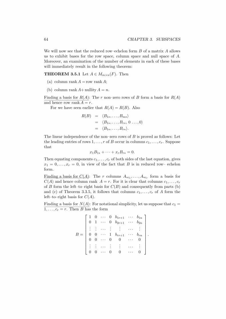
64 CHAPTER 3. SUBSPACES
We will now see that the reduced row–echelon form B of a matrix A allowsus to exhibit bases for the row space, column space and null space of A.Moreover, an examination of the number of elements in each of these baseswill immediately result in the following theorem:
THEOREM 3.5.1 Let A ∈ Mm×n(F ). Then
(a) column rankA = row rankA;
(b) column rankA+ nullityA = n.
Finding a basis for R(A): The r non–zero rows of B form a basis for R(A)and hence row rankA = r.
For we have seen earlier that R(A) = R(B). Also
R(B) = 〈B1∗, . . . , Bm∗〉= 〈B1∗, . . . , Br∗, 0 . . . , 0〉= 〈B1∗, . . . , Br∗〉.
The linear independence of the non–zero rows of B is proved as follows: Letthe leading entries of rows 1, . . . , r of B occur in columns c1, . . . , cr. Supposethat
x1B1∗ + · · · + xrBr∗ = 0.
Then equating components c1, . . . , cr of both sides of the last equation, givesx1 = 0, . . . , xr = 0, in view of the fact that B is in reduced row– echelonform.
Finding a basis for C(A): The r columns A∗c1 , . . . , A∗cr form a basis forC(A) and hence column rank A = r. For it is clear that columns c1, . . . , cr
of B form the left–to–right basis for C(B) and consequently from parts (b)and (c) of Theorem 3.3.5, it follows that columns c1, . . . , cr of A form theleft–to–right basis for C(A).
Finding a basis for N(A): For notational simplicity, let us suppose that c1 =1, . . . , cr = r. Then B has the form
B =
1 0 · · · 0 b1r+1 · · · b1n
0 1 · · · 0 b2r+1 · · · b2n...
... · · · ...... · · · ...
0 0 · · · 1 brr+1 · · · brn
0 0 · · · 0 0 · · · 0...
... · · · ...... · · · ...
0 0 · · · 0 0 · · · 0
.
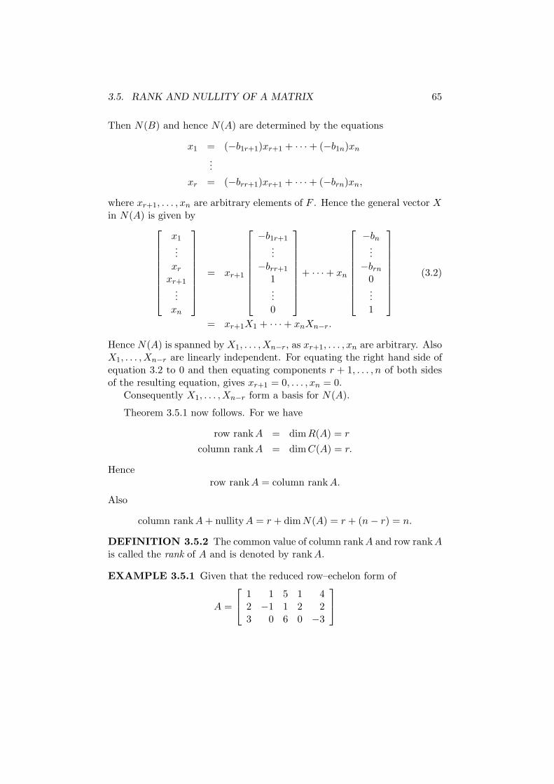
3.5. RANK AND NULLITY OF A MATRIX 65
Then N(B) and hence N(A) are determined by the equations
x1 = (−b1r+1)xr+1 + · · · + (−b1n)xn
...
xr = (−brr+1)xr+1 + · · · + (−brn)xn,
where xr+1, . . . , xn are arbitrary elements of F . Hence the general vector Xin N(A) is given by
x1...
xr
xr+1...
xn
= xr+1
−b1r+1...
−brr+1
1...0
+ · · · + xn
−bn...
−brn
0...1
(3.2)
= xr+1X1 + · · · + xnXn−r.
Hence N(A) is spanned by X1, . . . , Xn−r, as xr+1, . . . , xn are arbitrary. AlsoX1, . . . , Xn−r are linearly independent. For equating the right hand side ofequation 3.2 to 0 and then equating components r + 1, . . . , n of both sidesof the resulting equation, gives xr+1 = 0, . . . , xn = 0.
Consequently X1, . . . , Xn−r form a basis for N(A).
Theorem 3.5.1 now follows. For we have
row rankA = dim R(A) = r
column rankA = dim C(A) = r.
Hencerow rankA = column rankA.
Also
column rankA + nullityA = r + dimN(A) = r + (n − r) = n.
DEFINITION 3.5.2 The common value of column rankA and row rankAis called the rank of A and is denoted by rankA.
EXAMPLE 3.5.1 Given that the reduced row–echelon form of
A =
1 1 5 1 42 −1 1 2 23 0 6 0 −3
66 CHAPTER 3. SUBSPACES
equal to
B =
1 0 2 0 −10 1 3 0 20 0 0 1 3
,
find bases for R(A), C(A) and N(A).
Solution. [1, 0, 2, 0, −1], [0, 1, 3, 0, 2] and [0, 0, 0, 1, 3] form a basis forR(A). Also
A∗1 =
123
, A∗2 =
1−1
0
, A∗4 =
120
form a basis for C(A).Finally N(A) is given by
x1
x2
x3
x4
x5
=
−2x3 + x5
−3x3 − 2x5
x3
−3x5
x5
= x3
−2−3
100
+ x5
1−2
0−3
1
= x3X1 + x5X2,
where x3 and x5 are arbitrary. Hence X1 and X2 form a basis for N(A).Here rankA = 3 and nullityA = 2.
EXAMPLE 3.5.2 Let A =
[
1 22 4
]
. Then B =
[
1 20 0
]
is the reduced
row–echelon form of A.
Hence [1, 2] is a basis for R(A) and
[
12
]
is a basis for C(A). Also N(A)
is given by the equation x1 = −2x2, where x2 is arbitrary. Then[
x1
x2
]
=
[
−2x2
x2
]
= x2
[
−21
]
and hence
[
−21
]
is a basis for N(A).
Here rankA = 1 and nullityA = 1.
EXAMPLE 3.5.3 Let A =
[
1 23 4
]
. Then B =
[
1 00 1
]
is the reduced
row–echelon form of A.Hence [1, 0], [0, 1] form a basis for R(A) while [1, 3], [2, 4] form a basis
for C(A). Also N(A) = {0}.Here rankA = 2 and nullityA = 0.
3.6. PROBLEMS 67
We conclude this introduction to vector spaces with a result of greattheoretical importance.
THEOREM 3.5.2 Every linearly independent family of vectors in a sub-space S can be extended to a basis of S.
Proof. Suppose S has basis X1, . . . , Xm and that Y1, . . . , Yr is a linearlyindependent family of vectors in S. Then
S = 〈X1, . . . , Xm〉 = 〈Y1, . . . , Yr, X1, . . . , Xm〉,
as each of Y1, . . . , Yr is a linear combination of X1, . . . , Xm.Then applying the left–to–right algorithm to the second spanning family
for S will yield a basis for S which includes Y1, . . . , Yr.
3.6 PROBLEMS
1. Which of the following subsets of R2 are subspaces?
(a) [x, y] satisfying x = 2y;
(b) [x, y] satisfying x = 2y and 2x = y;
(c) [x, y] satisfying x = 2y + 1;
(d) [x, y] satisfying xy = 0;
(e) [x, y] satisfying x ≥ 0 and y ≥ 0.
[Answer: (a) and (b).]
2. If X, Y, Z are vectors in Rn, prove that
〈X, Y, Z〉 = 〈X + Y, X + Z, Y + Z〉.
3. Determine if X1 =
1012
, X2 =
0112
and X3 =
1113
are linearly
independent in R4.
4. For which real numbers λ are the following vectors linearly independentin R3?
X1 =
λ−1−1
, X2 =
−1λ
−1
, X3 =
−1−1
λ
.
68 CHAPTER 3. SUBSPACES
5. Find bases for the row, column and null spaces of the following matrixover Q:
A =
1 1 2 0 12 2 5 0 30 0 0 1 38 11 19 0 11
.
6. Find bases for the row, column and null spaces of the following matrixover Z2:
A =
1 0 1 0 10 1 0 1 11 1 1 1 00 0 1 1 0
.
7. Find bases for the row, column and null spaces of the following matrixover Z5:
A =
1 1 2 0 1 32 1 4 0 3 20 0 0 1 3 03 0 2 4 3 2
.
8. Find bases for the row, column and null spaces of the matrix A definedin section 1.6, Problem 17. (Note: In this question, F is a field of fourelements.)
9. If X1, . . . , Xm form a basis for a subspace S, prove that
X1, X1 + X2, . . . , X1 + · · · + Xm
also form a basis for S.
10. Let A =
[
a b c1 1 1
]
. Classify a, b, c such that (a) rankA = 1; (b)
rankA = 2.
[Answer: (a) a = b = c; (b) at least two of a, b, c are distinct.]
11. Let S be a subspace of Fn with dimS = m. If X1, . . . , Xm are vectorsin S with the property that S = 〈X1, . . . , Xm〉, prove that X1 . . . , Xm
form a basis for S.
12. Find a basis for the subspace S of R3 defined by the equation
x + 2y + 3z = 0.
3.6. PROBLEMS 69
Verify that Y1 = [−1, −1, 1]t ∈ S and find a basis for S which includesY1.
13. Let X1, . . . , Xm be vectors in Fn. If Xi = Xj , where i < j, prove thatX1, . . . Xm are linearly dependent.
14. Let X1, . . . , Xm+1 be vectors in Fn. Prove that
dim 〈X1, . . . , Xm+1〉 = dim 〈X1, . . . , Xm〉
if Xm+1 is a linear combination of X1, . . . , Xm, but
dim 〈X1, . . . , Xm+1〉 = dim 〈X1, . . . , Xm〉 + 1
if Xm+1 is not a linear combination of X1, . . . , Xm.
Deduce that the system of linear equations AX = B is consistent, ifand only if
rank [A|B] = rankA.
15. Let a1, . . . , an be elements of F , not all zero. Prove that the set ofvectors [x1, . . . , xn]t where x1, . . . , xn satisfy
a1x1 + · · · + anxn = 0
is a subspace of Fn with dimension equal to n − 1.
16. Prove Lemma 3.2.1, Theorem 3.2.1, Corollary 3.2.1 and Theorem 3.3.2.
17. Let R and S be subspaces of Fn, with R ⊆ S. Prove that
dim R ≤ dim S
and that equality implies R = S. (This is a very useful way of provingequality of subspaces.)
18. Let R and S be subspaces of Fn. If R ∪ S is a subspace of Fn, provethat R ⊆ S or S ⊆ R.
19. Let X1, . . . , Xr be a basis for a subspace S. Prove that all bases for Sare given by the family Y1, . . . , Yr, where
Yi =
r∑
j=1
aijXj ,
and where A = [aij ] ∈ Mr×r(F ) is a non–singular matrix.

70 CHAPTER 3. SUBSPACES
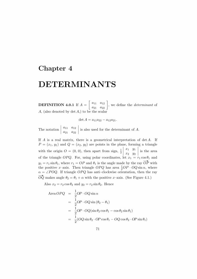
Chapter 4
DETERMINANTS
DEFINITION 4.0.1 If A =
[
a11 a12
a21 a22
]
, we define the determinant of
A, (also denoted by detA,) to be the scalar
det A = a11a22 − a12a21.
The notation
∣
∣
∣
∣
a11 a12
a21 a22
∣
∣
∣
∣
is also used for the determinant of A.
If A is a real matrix, there is a geometrical interpretation of detA. IfP = (x1, y1) and Q = (x2, y2) are points in the plane, forming a triangle
with the origin O = (0, 0), then apart from sign, 12
∣
∣
∣
∣
x1 y1
x2 y2
∣
∣
∣
∣
is the area
of the triangle OPQ. For, using polar coordinates, let x1 = r1 cos θ1 and
y1 = r1 sin θ1, where r1 = OP and θ1 is the angle made by the ray-
OP withthe positive x–axis. Then triangle OPQ has area 1
2OP · OQ sinα, whereα = ∠POQ. If triangle OPQ has anti–clockwise orientation, then the ray-
OQ makes angle θ2 = θ1 + α with the positive x–axis. (See Figure 4.1.)
Also x2 = r2 cos θ2 and y2 = r2 sin θ2. Hence
Area OPQ =1
2OP · OQ sinα
=1
2OP · OQ sin (θ2 − θ1)
=1
2OP · OQ(sin θ2 cos θ1 − cos θ2 sin θ1)
=1
2(OQ sin θ2 · OP cos θ1 − OQ cos θ2 · OP sin θ1)
71

72 CHAPTER 4. DETERMINANTS
-
6
x
y
©©©©©©©©
Q
P
O
θ1
α
¢¢¢¢¢¢¢¢@
@@
@
Figure 4.1: Area of triangle OPQ.
=1
2(y2x1 − x2y1)
=1
2
∣
∣
∣
∣
x1 y1
x2 y2
∣
∣
∣
∣
.
Similarly, if triangle OPQ has clockwise orientation, then its area equals
−12
∣
∣
∣
∣
x1 y1
x2 y2
∣
∣
∣
∣
.
For a general triangle P1P2P3, with Pi = (xi, yi), i = 1, 2, 3, we cantake P1 as the origin. Then the above formula gives
1
2
∣
∣
∣
∣
x2 − x1 y2 − y1
x3 − x1 y3 − y1
∣
∣
∣
∣
or − 1
2
∣
∣
∣
∣
x2 − x1 y2 − y1
x3 − x1 y3 − y1
∣
∣
∣
∣
,
according as vertices P1P2P3 are anti–clockwise or clockwise oriented.
We now give a recursive definition of the determinant of an n×n matrixA = [aij ], n ≥ 3.
DEFINITION 4.0.2 (Minor) Let Mij(A) (or simply Mij if there is noambiguity) denote the determinant of the (n − 1) × (n − 1) submatrix of Aformed by deleting the i–th row and j–th column of A. (Mij(A) is calledthe (i, j) minor of A.)
Assume that the determinant function has been defined for matrices ofsize (n−1)×(n−1). Then detA is defined by the so–called first–row Laplace
73
expansion:
detA = a11M11(A) − a12M12(A) + . . . + (−1)1+nM1n(A)
=n
∑
j=1
(−1)1+ja1jM1j(A).
For example, if A = [aij ] is a 3 × 3 matrix, the Laplace expansion gives
det A = a11M11(A) − a12M12(A) + a13M13(A)
= a11
∣
∣
∣
∣
a22 a23
a32 a33
∣
∣
∣
∣
− a12
∣
∣
∣
∣
a21 a23
a31 a33
∣
∣
∣
∣
+ a13
∣
∣
∣
∣
a21 a22
a31 a32
∣
∣
∣
∣
= a11(a22a33 − a23a32) − a12(a21a33 − a23a31) + a13(a21a32 − a22a31)= a11a22a33 − a11a23a32 − a12a21a33 + a12a23a31 + a13a21a32 − a13a22a31.
The recursive definition also works for 2 × 2 determinants, if we define thedeterminant of a 1 × 1 matrix [t] to be the scalar t:
detA = a11M11(A) − a12M12(A) = a11a22 − a12a21.
EXAMPLE 4.0.1 If P1P2P3 is a triangle with Pi = (xi, yi), i = 1, 2, 3,then the area of triangle P1P2P3 is
1
2
∣
∣
∣
∣
∣
∣
x1 y1 1x2 y2 1x3 y3 1
∣
∣
∣
∣
∣
∣
or − 1
2
∣
∣
∣
∣
∣
∣
x1 y1 1x2 y2 1x3 y3 1
∣
∣
∣
∣
∣
∣
,
according as the orientation of P1P2P3 is anti–clockwise or clockwise.
For from the definition of 3 × 3 determinants, we have
1
2
∣
∣
∣
∣
∣
∣
x1 y1 1x2 y2 1x3 y3 1
∣
∣
∣
∣
∣
∣
=1
2
(
x1
∣
∣
∣
∣
y2 1y3 1
∣
∣
∣
∣
− y1
∣
∣
∣
∣
x2 1x3 1
∣
∣
∣
∣
+
∣
∣
∣
∣
x2 y2
x3 y3
∣
∣
∣
∣
)
=1
2
∣
∣
∣
∣
x2 − x1 y2 − y1
x3 − x1 y3 − y1
∣
∣
∣
∣
.
One property of determinants that follows immediately from the defini-tion is the following:
THEOREM 4.0.1 If a row of a matrix is zero, then the value of the de-terminant is zero.
74 CHAPTER 4. DETERMINANTS
(The corresponding result for columns also holds, but here a simple proofby induction is needed.)
One of the simplest determinants to evaluate is that of a lower triangularmatrix.
THEOREM 4.0.2 Let A = [aij ], where aij = 0 if i < j. Then
det A = a11a22 . . . ann. (4.1)
An important special case is when A is a diagonal matrix.If A =diag (a1, . . . , an) then detA = a1 . . . an. In particular, for a scalar
matrix tIn, we have det (tIn) = tn.
Proof. Use induction on the size n of the matrix.The result is true for n = 2. Now let n > 2 and assume the result true
for matrices of size n − 1. If A is n × n, then expanding detA along row 1gives
det A = a11
∣
∣
∣
∣
∣
∣
∣
∣
∣
a22 0 . . . 0a32 a33 . . . 0...
an1 an2 . . . ann
∣
∣
∣
∣
∣
∣
∣
∣
∣
= a11(a22 . . . ann)
by the induction hypothesis.
If A is upper triangular, equation 4.1 remains true and the proof is againan exercise in induction, with the slight difference that the column versionof theorem 4.0.1 is needed.
REMARK 4.0.1 It can be shown that the expanded form of the determi-nant of an n × n matrix A consists of n! signed products ±a1i1a2i2 . . . anin ,where (i1, i2, . . . , in) is a permutation of (1, 2, . . . , n), the sign being 1 or−1, according as the number of inversions of (i1, i2, . . . , in) is even or odd.An inversion occurs when ir > is but r < s. (The proof is not easy and isomitted.)
The definition of the determinant of an n × n matrix was given in termsof the first–row expansion. The next theorem says that we can expandthe determinant along any row or column. (The proof is not easy and isomitted.)
75
THEOREM 4.0.3
det A =n
∑
j=1
(−1)i+jaijMij(A)
for i = 1, . . . , n (the so–called i–th row expansion) and
det A =n
∑
i=1
(−1)i+jaijMij(A)
for j = 1, . . . , n (the so–called j–th column expansion).
REMARK 4.0.2 The expression (−1)i+j obeys the chess–board patternof signs:
+ − + . . .− + − . . .+ − + . . ....
.
The following theorems can be proved by straightforward inductions onthe size of the matrix:
THEOREM 4.0.4 A matrix and its transpose have equal determinants;that is
det At = det A.
THEOREM 4.0.5 If two rows of a matrix are equal, the determinant iszero. Similarly for columns.
THEOREM 4.0.6 If two rows of a matrix are interchanged, the determi-nant changes sign.
EXAMPLE 4.0.2 If P1 = (x1, y1) and P2 = (x2, y2) are distinct points,then the line through P1 and P2 has equation
∣
∣
∣
∣
∣
∣
x y 1x1 y1 1x2 y2 1
∣
∣
∣
∣
∣
∣
= 0.
76 CHAPTER 4. DETERMINANTS
For, expanding the determinant along row 1, the equation becomes
ax + by + c = 0,
where
a =
∣
∣
∣
∣
y1 1y2 1
∣
∣
∣
∣
= y1 − y2 and b = −∣
∣
∣
∣
x1 1x2 1
∣
∣
∣
∣
= x2 − x1.
This represents a line, as not both a and b can be zero. Also this line passesthrough Pi, i = 1, 2. For the determinant has its first and i–th rows equalif x = xi and y = yi and is consequently zero.
There is a corresponding formula in three–dimensional geometry. IfP1, P2, P3 are non–collinear points in three–dimensional space, with Pi =(xi, yi, zi), i = 1, 2, 3, then the equation
∣
∣
∣
∣
∣
∣
∣
∣
x y z 1x1 y1 z1 1x2 y2 z2 1x3 y3 z3 1
∣
∣
∣
∣
∣
∣
∣
∣
= 0
represents the plane through P1, P2, P3. For, expanding the determinantalong row 1, the equation becomes ax + by + cz + d = 0, where
a =
∣
∣
∣
∣
∣
∣
y1 z1 1y2 z2 1y3 z3 1
∣
∣
∣
∣
∣
∣
, b = −
∣
∣
∣
∣
∣
∣
x1 z1 1x2 z2 1x3 z3 1
∣
∣
∣
∣
∣
∣
, c =
∣
∣
∣
∣
∣
∣
x1 y1 1x2 y2 1x3 y3 1
∣
∣
∣
∣
∣
∣
.
As we shall see in chapter 6, this represents a plane if at least one of a, b, cis non–zero. However, apart from sign and a factor 1
2 , the determinantexpressions for a, b, c give the values of the areas of projections of triangleP1P2P3 on the (y, z), (x, z) and (x, y) planes, respectively. Geometrically,it is then clear that at least one of a, b, c is non–zero. It is also possible togive an algebraic proof of this fact.
Finally, the plane passes through Pi, i = 1, 2, 3 as the determinant hasits first and i–th rows equal if x = xi, y = yi, z = zi and is consequentlyzero. We now work towards proving that a matrix is non–singular if itsdeterminant is non–zero.
DEFINITION 4.0.3 (Cofactor) The (i, j) cofactor of A, denoted byCij(A) (or Cij if there is no ambiguity) is defined by
Cij(A) = (−1)i+jMij(A).
77
REMARK 4.0.3 It is important to notice that Cij(A), like Mij(A), doesnot depend on aij . Use will be made of this observation presently.
In terms of the cofactor notation, Theorem 4.0.3 takes the form
THEOREM 4.0.7
det A =n
∑
j=1
aijCij(A)
for i = 1, . . . , n and
det A =n
∑
i=1
aijCij(A)
for j = 1, . . . , n.
Another result involving cofactors is
THEOREM 4.0.8 Let A be an n × n matrix. Then
(a)n
∑
j=1
aijCkj(A) = 0 if i 6= k.
Also
(b)n
∑
i=1
aijCik(A) = 0 if j 6= k.
Proof.If A is n×n and i 6= k, let B be the matrix obtained from A by replacing
row k by row i. Then detB = 0 as B has two identical rows.Now expand detB along row k. We get
0 = detB =n
∑
j=1
bkjCkj(B)
=n
∑
j=1
aijCkj(A),
in view of Remark 4.0.3.
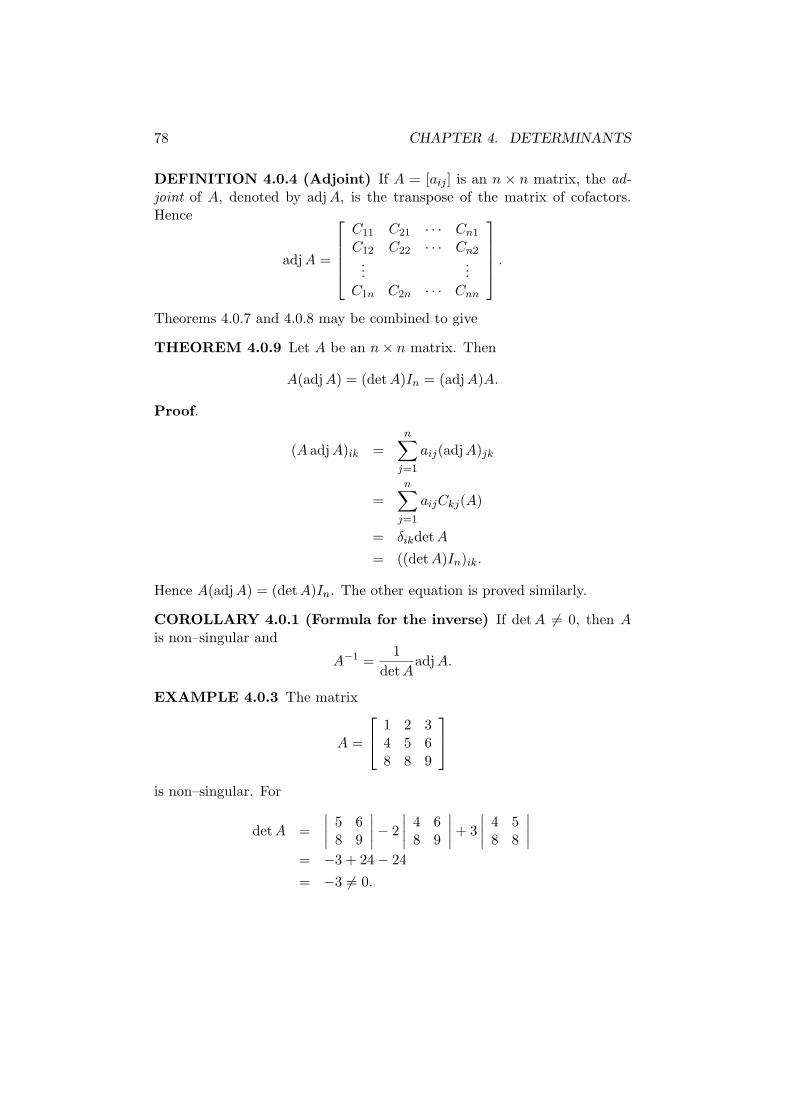
78 CHAPTER 4. DETERMINANTS
DEFINITION 4.0.4 (Adjoint) If A = [aij ] is an n × n matrix, the ad-
joint of A, denoted by adjA, is the transpose of the matrix of cofactors.Hence
adjA =
C11 C21 · · · Cn1
C12 C22 · · · Cn2...
...C1n C2n · · · Cnn
.
Theorems 4.0.7 and 4.0.8 may be combined to give
THEOREM 4.0.9 Let A be an n × n matrix. Then
A(adj A) = (det A)In = (adjA)A.
Proof.
(A adjA)ik =n
∑
j=1
aij(adjA)jk
=n
∑
j=1
aijCkj(A)
= δikdetA
= ((det A)In)ik.
Hence A(adj A) = (det A)In. The other equation is proved similarly.
COROLLARY 4.0.1 (Formula for the inverse) If detA 6= 0, then Ais non–singular and
A−1 =1
det AadjA.
EXAMPLE 4.0.3 The matrix
A =
1 2 34 5 68 8 9
is non–singular. For
detA =
∣
∣
∣
∣
5 68 9
∣
∣
∣
∣
− 2
∣
∣
∣
∣
4 68 9
∣
∣
∣
∣
+ 3
∣
∣
∣
∣
4 58 8
∣
∣
∣
∣
= −3 + 24 − 24
= −3 6= 0.
79
Also
A−1 =1
−3
C11 C21 C31
C12 C22 C32
C13 C23 C33
= −1
3
∣
∣
∣
∣
5 68 9
∣
∣
∣
∣
−∣
∣
∣
∣
2 38 9
∣
∣
∣
∣
∣
∣
∣
∣
2 35 6
∣
∣
∣
∣
−∣
∣
∣
∣
4 68 9
∣
∣
∣
∣
∣
∣
∣
∣
1 38 9
∣
∣
∣
∣
−∣
∣
∣
∣
1 34 6
∣
∣
∣
∣
∣
∣
∣
∣
4 58 8
∣
∣
∣
∣
−∣
∣
∣
∣
1 28 8
∣
∣
∣
∣
∣
∣
∣
∣
1 24 5
∣
∣
∣
∣
= −1
3
−3 6 −312 −15 6−8 8 −3
.
The following theorem is useful for simplifying and numerically evaluatinga determinant. Proofs are obtained by expanding along the correspondingrow or column.
THEOREM 4.0.10 The determinant is a linear function of each row andcolumn. For example
(a)
˛
˛
˛
˛
˛
˛
a11 + a′
11 a12 + a′
12 a13 + a′
13a21 a22 a23
a31 a32 a33
˛
˛
˛
˛
˛
˛
=
˛
˛
˛
˛
˛
˛
a11 a12 a13
a21 a22 a23
a31 a32 a33
˛
˛
˛
˛
˛
˛
+
˛
˛
˛
˛
˛
˛
a′
11 a′
12 a′
13a21 a22 a23
a31 a32 a33
˛
˛
˛
˛
˛
˛
(b)
˛
˛
˛
˛
˛
˛
ta11 ta12 ta13
a21 a22 a23
a31 a32 a33
˛
˛
˛
˛
˛
˛
= t
˛
˛
˛
˛
˛
˛
a11 a12 a13
a21 a22 a23
a31 a32 a33
˛
˛
˛
˛
˛
˛
.
COROLLARY 4.0.2 If a multiple of a row is added to another row, thevalue of the determinant is unchanged. Similarly for columns.
Proof. We illustrate with a 3 × 3 example, but the proof is really quitegeneral.
˛
˛
˛
˛
˛
˛
a11 + ta21 a12 + ta22 a13 + ta23
a21 a22 a23
a31 a32 a33
˛
˛
˛
˛
˛
˛
=
˛
˛
˛
˛
˛
˛
a11 a12 a13
a21 a22 a23
a31 a32 a33
˛
˛
˛
˛
˛
˛
+
˛
˛
˛
˛
˛
˛
ta21 ta22 ta23
a21 a22 a23
a31 a32 a33
˛
˛
˛
˛
˛
˛
=
˛
˛
˛
˛
˛
˛
a11 a12 a13
a21 a22 a23
a31 a32 a33
˛
˛
˛
˛
˛
˛
+ t
˛
˛
˛
˛
˛
˛
a21 a22 a23
a21 a22 a23
a31 a32 a33
˛
˛
˛
˛
˛
˛
=
˛
˛
˛
˛
˛
˛
a11 a12 a13
a21 a22 a23
a31 a32 a33
˛
˛
˛
˛
˛
˛
+ t × 0
=
˛
˛
˛
˛
˛
˛
a11 a12 a13
a21 a22 a23
a31 a32 a33
˛
˛
˛
˛
˛
˛
.
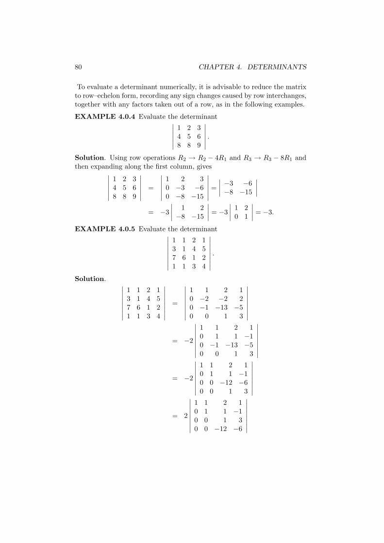
80 CHAPTER 4. DETERMINANTS
To evaluate a determinant numerically, it is advisable to reduce the matrixto row–echelon form, recording any sign changes caused by row interchanges,together with any factors taken out of a row, as in the following examples.
EXAMPLE 4.0.4 Evaluate the determinant∣
∣
∣
∣
∣
∣
1 2 34 5 68 8 9
∣
∣
∣
∣
∣
∣
.
Solution. Using row operations R2 → R2 − 4R1 and R3 → R3 − 8R1 andthen expanding along the first column, gives
∣
∣
∣
∣
∣
∣
1 2 34 5 68 8 9
∣
∣
∣
∣
∣
∣
=
∣
∣
∣
∣
∣
∣
1 2 30 −3 −60 −8 −15
∣
∣
∣
∣
∣
∣
=
∣
∣
∣
∣
−3 −6−8 −15
∣
∣
∣
∣
= −3
∣
∣
∣
∣
1 2−8 −15
∣
∣
∣
∣
= −3
∣
∣
∣
∣
1 20 1
∣
∣
∣
∣
= −3.
EXAMPLE 4.0.5 Evaluate the determinant∣
∣
∣
∣
∣
∣
∣
∣
1 1 2 13 1 4 57 6 1 21 1 3 4
∣
∣
∣
∣
∣
∣
∣
∣
.
Solution.∣
∣
∣
∣
∣
∣
∣
∣
1 1 2 13 1 4 57 6 1 21 1 3 4
∣
∣
∣
∣
∣
∣
∣
∣
=
∣
∣
∣
∣
∣
∣
∣
∣
1 1 2 10 −2 −2 20 −1 −13 −50 0 1 3
∣
∣
∣
∣
∣
∣
∣
∣
= −2
∣
∣
∣
∣
∣
∣
∣
∣
1 1 2 10 1 1 −10 −1 −13 −50 0 1 3
∣
∣
∣
∣
∣
∣
∣
∣
= −2
∣
∣
∣
∣
∣
∣
∣
∣
1 1 2 10 1 1 −10 0 −12 −60 0 1 3
∣
∣
∣
∣
∣
∣
∣
∣
= 2
∣
∣
∣
∣
∣
∣
∣
∣
1 1 2 10 1 1 −10 0 1 30 0 −12 −6
∣
∣
∣
∣
∣
∣
∣
∣
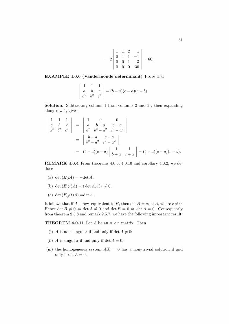
81
= 2
∣
∣
∣
∣
∣
∣
∣
∣
1 1 2 10 1 1 −10 0 1 30 0 0 30
∣
∣
∣
∣
∣
∣
∣
∣
= 60.
EXAMPLE 4.0.6 (Vandermonde determinant) Prove that
∣
∣
∣
∣
∣
∣
1 1 1a b ca2 b2 c2
∣
∣
∣
∣
∣
∣
= (b − a)(c − a)(c − b).
Solution. Subtracting column 1 from columns 2 and 3 , then expandingalong row 1, gives
∣
∣
∣
∣
∣
∣
1 1 1a b ca2 b2 c2
∣
∣
∣
∣
∣
∣
=
∣
∣
∣
∣
∣
∣
1 0 0a b − a c − aa2 b2 − a2 c2 − a2
∣
∣
∣
∣
∣
∣
=
∣
∣
∣
∣
b − a c − ab2 − a2 c2 − a2
∣
∣
∣
∣
= (b − a)(c − a)
∣
∣
∣
∣
1 1b + a c + a
∣
∣
∣
∣
= (b − a)(c − a)(c − b).
REMARK 4.0.4 From theorems 4.0.6, 4.0.10 and corollary 4.0.2, we de-duce
(a) det (EijA) = −detA,
(b) det (Ei(t)A) = t det A, if t 6= 0,
(c) det (Eij(t)A) =detA.
It follows that if A is row–equivalent to B, then detB = c det A, where c 6= 0.Hence det B 6= 0 ⇔ det A 6= 0 and detB = 0 ⇔ det A = 0. Consequentlyfrom theorem 2.5.8 and remark 2.5.7, we have the following important result:
THEOREM 4.0.11 Let A be an n × n matrix. Then
(i) A is non–singular if and only if detA 6= 0;
(ii) A is singular if and only if detA = 0;
(iii) the homogeneous system AX = 0 has a non–trivial solution if andonly if detA = 0.
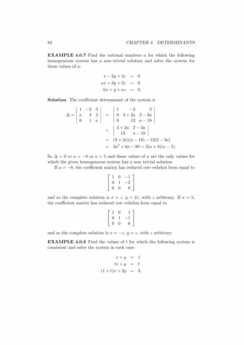
82 CHAPTER 4. DETERMINANTS
EXAMPLE 4.0.7 Find the rational numbers a for which the followinghomogeneous system has a non–trivial solution and solve the system forthese values of a:
x − 2y + 3z = 0
ax + 3y + 2z = 0
6x + y + az = 0.
Solution. The coefficient determinant of the system is
∆ =
∣
∣
∣
∣
∣
∣
1 −2 3a 3 26 1 a
∣
∣
∣
∣
∣
∣
=
∣
∣
∣
∣
∣
∣
1 −2 30 3 + 2a 2 − 3a0 13 a − 18
∣
∣
∣
∣
∣
∣
=
∣
∣
∣
∣
3 + 2a 2 − 3a13 a − 18
∣
∣
∣
∣
= (3 + 2a)(a − 18) − 13(2 − 3a)
= 2a2 + 6a − 80 = 2(a + 8)(a − 5).
So ∆ = 0 ⇔ a = −8 or a = 5 and these values of a are the only values forwhich the given homogeneous system has a non–trivial solution.
If a = −8, the coefficient matrix has reduced row–echelon form equal to
1 0 −10 1 −20 0 0
and so the complete solution is x = z, y = 2z, with z arbitrary. If a = 5,the coefficient matrix has reduced row–echelon form equal to
1 0 10 1 −10 0 0
and so the complete solution is x = −z, y = z, with z arbitrary.
EXAMPLE 4.0.8 Find the values of t for which the following system isconsistent and solve the system in each case:
x + y = 1
tx + y = t
(1 + t)x + 2y = 3.
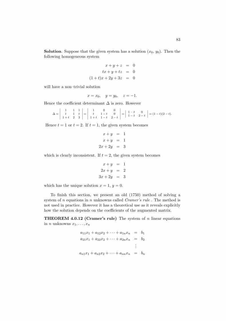
83
Solution. Suppose that the given system has a solution (x0, y0). Then thefollowing homogeneous system
x + y + z = 0
tx + y + tz = 0
(1 + t)x + 2y + 3z = 0
will have a non–trivial solution
x = x0, y = y0, z = −1.
Hence the coefficient determinant ∆ is zero. However
∆ =
˛
˛
˛
˛
˛
˛
1 1 1t 1 t
1 + t 2 3
˛
˛
˛
˛
˛
˛
=
˛
˛
˛
˛
˛
˛
1 0 0t 1 − t 0
1 + t 1 − t 2 − t
˛
˛
˛
˛
˛
˛
=
˛
˛
˛
˛
1 − t 01 − t 2 − t
˛
˛
˛
˛
= (1 − t)(2 − t).
Hence t = 1 or t = 2. If t = 1, the given system becomes
x + y = 1
x + y = 1
2x + 2y = 3
which is clearly inconsistent. If t = 2, the given system becomes
x + y = 1
2x + y = 2
3x + 2y = 3
which has the unique solution x = 1, y = 0.
To finish this section, we present an old (1750) method of solving asystem of n equations in n unknowns called Cramer’s rule . The method isnot used in practice. However it has a theoretical use as it reveals explicitlyhow the solution depends on the coefficients of the augmented matrix.
THEOREM 4.0.12 (Cramer’s rule) The system of n linear equationsin n unknowns x1, . . . , xn
a11x1 + a12x2 + · · · + a1nxn = b1
a21x1 + a22x2 + · · · + a2nxn = b2
...
an1x1 + an2x2 + · · · + annxn = bn
84 CHAPTER 4. DETERMINANTS
has a unique solution if ∆ = det [aij ] 6= 0, namely
x1 =∆1
∆, x2 =
∆2
∆, . . . , xn =
∆n
∆,
where ∆i is the determinant of the matrix formed by replacing the i–thcolumn of the coefficient matrix A by the entries b1, b2, . . . , bn.
Proof. Suppose the coefficient determinant ∆ 6= 0. Then by corollary 4.0.1,A−1 exists and is given by A−1 = 1
∆ adjA and the system has the uniquesolution
x1
x2...
xn
= A−1
b1
b2...
bn
=1
∆
C11 C21 · · · Cn1
C12 C22 · · · Cn2...
...C1n C2n · · · Cnn
b1
b2...
bn
=1
∆
b1C11 + b2C21 + . . . + bnCn1
b2C12 + b2C22 + . . . + bnCn2...
bnC1n + b2C2n + . . . + bnCnn
.
However the i–th component of the last vector is the expansion of ∆i alongcolumn i. Hence
x1
x2...
xn
=1
∆
∆1
∆2...
∆n
=
∆1/∆∆2/∆
...∆n/∆
.
4.1 PROBLEMS
.
1. If the points Pi = (xi, yi), i = 1, 2, 3, 4 form a quadrilateral with ver-tices in anti–clockwise orientation, prove that the area of the quadri-lateral equals
1
2
(∣
∣
∣
∣
x1 x2
y1 y2
∣
∣
∣
∣
+
∣
∣
∣
∣
x2 x3
y2 y3
∣
∣
∣
∣
+
∣
∣
∣
∣
x3 x4
y3 y4
∣
∣
∣
∣
+
∣
∣
∣
∣
x4 x1
y4 y1
∣
∣
∣
∣
)
.
(This formula generalizes to a simple polygon and is known as theSurveyor’s formula.)
4.1. PROBLEMS 85
2. Prove that the following identity holds by expressing the left–handside as the sum of 8 determinants:
∣
∣
∣
∣
∣
∣
a + x b + y c + zx + u y + v z + wu + a v + b w + c
∣
∣
∣
∣
∣
∣
= 2
∣
∣
∣
∣
∣
∣
a b cx y zu v w
∣
∣
∣
∣
∣
∣
.
3. Prove that∣
∣
∣
∣
∣
∣
n2 (n + 1)2 (n + 2)2
(n + 1)2 (n + 2)2 (n + 3)2
(n + 2)2 (n + 3)2 (n + 4)2
∣
∣
∣
∣
∣
∣
= −8.
4. Evaluate the following determinants:
(a)
∣
∣
∣
∣
∣
∣
246 427 3271014 543 443−342 721 621
∣
∣
∣
∣
∣
∣
(b)
∣
∣
∣
∣
∣
∣
∣
∣
1 2 3 4−2 1 −4 3
3 −4 −1 24 3 −2 −1
∣
∣
∣
∣
∣
∣
∣
∣
.
[Answers: (a) −29400000; (b) 900.]
5. Compute the inverse of the matrix
A =
1 0 −23 1 45 2 −3
by first computing the adjoint matrix.
[Answer: A−1 = −113
−11 −4 229 7 −101 −2 1
.]
6. Prove that the following identities hold:
(i)
∣
∣
∣
∣
∣
∣
2a 2b b − c2b 2a a + c
a + b a + b b
∣
∣
∣
∣
∣
∣
= −2(a − b)2(a + b),
(ii)
∣
∣
∣
∣
∣
∣
b + c b cc c + a ab a a + b
∣
∣
∣
∣
∣
∣
= 2a(b2 + c2).
86 CHAPTER 4. DETERMINANTS
7. Let Pi = (xi, yi), i = 1, 2, 3. If x1, x2, x3 are distinct, prove that thereis precisely one curve of the form y = ax2 + bx + c passing throughP1, P2 and P3.
8. Let
A =
1 1 −12 3 k1 k 3
.
Find the values of k for which detA = 0 and hence, or otherwise,determine the value of k for which the following system has more thanone solution:
x + y − z = 1
2x + 3y + kz = 3
x + ky + 3z = 2.
Solve the system for this value of k and determine the solution forwhich x2 + y2 + z2 has least value.
[Answer: k = 2; x = 10/21, y = 13/21, z = 2/21.]
9. By considering the coefficient determinant, find all rational numbers aand b for which the following system has (i) no solutions, (ii) exactlyone solution, (iii) infinitely many solutions:
x − 2y + bz = 3
ax + 2z = 2
5x + 2y = 1.
Solve the system in case (iii).
[Answer: (i) ab = 12 and a 6= 3, no solution; ab 6= 12, unique solution;a = 3, b = 4, infinitely many solutions; x = −2
3z + 23 , y = 5
3z− 76 , with
z arbitrary.]
10. Express the determinant of the matrix
B =
1 1 2 11 2 3 42 4 7 2t + 62 2 6 − t t
4.1. PROBLEMS 87
as as polynomial in t and hence determine the rational values of t forwhich B−1 exists.
[Answer: detB = (t − 2)(2t − 1); t 6= 2 and t 6= 12 .]
11. If A is a 3 × 3 matrix over a field and detA 6= 0, prove that
(i) det (adjA) = (det A)2,
(ii) (adjA)−1 =1
detAA = adj (A−1).
12. Suppose that A is a real 3 × 3 matrix such that AtA = I3.
(i) Prove that At(A − I3) = −(A − I3)t.
(ii) Prove that detA = ±1.
(iii) Use (i) to prove that if detA = 1, then det (A − I3) = 0.
13. If A is a square matrix such that one column is a linear combination ofthe remaining columns, prove that detA = 0. Prove that the conversealso holds.
14. Use Cramer’s rule to solve the system
−2x + 3y − z = 1x + 2y − z = 4
−2x − y + z = −3.
[Answer: x = 2, y = 3, z = 4.]
15. Use remark 4.0.4 to deduce that
detEij = −1, det Ei(t) = t, det Eij(t) = 1
and use theorem 2.5.8 and induction, to prove that
det (BA) = det B det A,
if B is non–singular. Also prove that the formula holds when B issingular.
16. Prove that∣
∣
∣
∣
∣
∣
∣
∣
a + b + c a + b a aa + b a + b + c a a
a a a + b + c a + ba a a + b a + b + c
∣
∣
∣
∣
∣
∣
∣
∣
= c2(2b+c)(4a+2b+c).
88 CHAPTER 4. DETERMINANTS
17. Prove that∣
∣
∣
∣
∣
∣
∣
∣
1 + u1 u1 u1 u1
u2 1 + u2 u2 u2
u3 u3 1 + u3 u3
u4 u4 u4 1 + u4
∣
∣
∣
∣
∣
∣
∣
∣
= 1 + u1 + u2 + u3 + u4.
18. Let A ∈ Mn×n(F ). If At = −A, prove that detA = 0 if n is odd and1 + 1 6= 0 in F .
19. Prove that∣
∣
∣
∣
∣
∣
∣
∣
1 1 1 1r 1 1 1r r 1 1r r r 1
∣
∣
∣
∣
∣
∣
∣
∣
= (1 − r)3.
20. Express the determinant
∣
∣
∣
∣
∣
∣
1 a2 − bc a4
1 b2 − ca b4
1 c2 − ab c4
∣
∣
∣
∣
∣
∣
as the product of one quadratic and four linear factors.
[Answer: (b − a)(c − a)(c − b)(a + b + c)(b2 + bc + c2 + ac + ab + a2).]
Chapter 5
COMPLEX NUMBERS
5.1 Constructing the complex numbers
One way of introducing the field C of complex numbers is via the arithmeticof 2 × 2 matrices.
DEFINITION 5.1.1 A complex number is a matrix of the form
[
x −yy x
]
,
where x and y are real numbers.
Complex numbers of the form
[
x 00 x
]
are scalar matrices and are called
real complex numbers and are denoted by the symbol {x}.The real complex numbers {x} and {y} are respectively called the real
part and imaginary part of the complex number
[
x −yy x
]
.
The complex number
[
0 −11 0
]
is denoted by the symbol i.
We have the identities[
x −yy x
]
=
[
x 00 x
]
+
[
0 −yy 0
]
=
[
x 00 x
]
+
[
0 −11 0
] [
y 00 y
]
= {x} + i{y},
i2 =
[
0 −11 0
] [
0 −11 0
]
=
[
−1 00 −1
]
= {−1}.
89

90 CHAPTER 5. COMPLEX NUMBERS
Complex numbers of the form i{y}, where y is a non–zero real number, arecalled imaginary numbers.
If two complex numbers are equal, we can equate their real and imaginaryparts:
{x1} + i{y1} = {x2} + i{y2} ⇒ x1 = x2 and y1 = y2,
if x1, x2, y1, y2 are real numbers. Noting that {0} + i{0} = {0}, gives theuseful special case is
{x} + i{y} = {0} ⇒ x = 0 and y = 0,
if x and y are real numbers.The sum and product of two real complex numbers are also real complex
numbers:{x} + {y} = {x + y}, {x}{y} = {xy}.
Also, as real complex numbers are scalar matrices, their arithmetic is verysimple. They form a field under the operations of matrix addition andmultiplication. The additive identity is {0}, the additive inverse of {x} is{−x}, the multiplicative identity is {1} and the multiplicative inverse of {x}is {x−1}. Consequently
{x} − {y} = {x} + (−{y}) = {x} + {−y} = {x − y},
{x}{y} = {x}{y}−1 = {x}{y−1} = {xy−1} =
{
x
y
}
.
It is customary to blur the distinction between the real complex number{x} and the real number x and write {x} as x. Thus we write the complexnumber {x} + i{y} simply as x + iy.
More generally, the sum of two complex numbers is a complex number:
(x1 + iy1) + (x2 + iy2) = (x1 + x2) + i(y1 + y2); (5.1)
and (using the fact that scalar matrices commute with all matrices undermatrix multiplication and {−1}A = −A if A is a matrix), the product oftwo complex numbers is a complex number:
(x1 + iy1)(x2 + iy2) = x1(x2 + iy2) + (iy1)(x2 + iy2)
= x1x2 + x1(iy2) + (iy1)x2 + (iy1)(iy2)
= x1x2 + ix1y2 + iy1x2 + i2y1y2
= (x1x2 + {−1}y1y2) + i(x1y2 + y1x2)
= (x1x2 − y1y2) + i(x1y2 + y1x2), (5.2)
5.2. CALCULATING WITH COMPLEX NUMBERS 91
The set C of complex numbers forms a field under the operations ofmatrix addition and multiplication. The additive identity is 0, the additiveinverse of x + iy is the complex number (−x) + i(−y), the multiplicativeidentity is 1 and the multiplicative inverse of the non–zero complex numberx + iy is the complex number u + iv, where
u =x
x2 + y2and v =
−y
x2 + y2.
(If x + iy 6= 0, then x 6= 0 or y 6= 0, so x2 + y2 6= 0.)
From equations 5.1 and 5.2, we observe that addition and multiplicationof complex numbers is performed just as for real numbers, replacing i2 by−1, whenever it occurs.
A useful identity satisfied by complex numbers is
r2 + s2 = (r + is)(r − is).
This leads to a method of expressing the ratio of two complex numbers inthe form x + iy, where x and y are real complex numbers.
x1 + iy1
x2 + iy2=
(x1 + iy1)(x2 − iy2)
(x2 + iy2)(x2 − iy2)
=(x1x2 + y1y2) + i(−x1y2 + y1x2)
x22 + y2
2
.
The process is known as rationalization of the denominator.
5.2 Calculating with complex numbers
We can now do all the standard linear algebra calculations over the field ofcomplex numbers – find the reduced row–echelon form of an matrix whose el-ements are complex numbers, solve systems of linear equations, find inversesand calculate determinants.
For example, solve the system
(1 + i)z + (2 − i)w = 2 + 7i
7z + (8 − 2i)w = 4 − 9i.
The coefficient determinant is∣
∣
∣
∣
1 + i 2 − i7 8 − 2i
∣
∣
∣
∣
= (1 + i)(8 − 2i) − 7(2 − i)
= (8 − 2i) + i(8 − 2i) − 14 + 7i
= −4 + 13i 6= 0.
92 CHAPTER 5. COMPLEX NUMBERS
Hence by Cramer’s rule, there is a unique solution:
z =
∣
∣
∣
∣
2 + 7i 2 − i4 − 9i 8 − 2i
∣
∣
∣
∣
−4 + 13i
=(2 + 7i)(8 − 2i) − (4 − 9i)(2 − i)
−4 + 13i
=2(8 − 2i) + (7i)(8 − 2i) − {(4(2 − i) − 9i(2 − i)}
−4 + 13i
=16 − 4i + 56i − 14i2 − {8 − 4i − 18i + 9i2}
−4 + 13i
=31 + 74i
−4 + 13i
=(31 + 74i)(−4 − 13i)
(−4)2 + 132
=838 − 699i
(−4)2 + 132
=838
185− 699
185i
and similarly w =−698
185+
229
185i.
An important property enjoyed by complex numbers is that every com-plex number has a square root.
THEOREM 5.2.1 If w is a non–zero complex number, then the equationz2 = w has a solution z ∈ C.
Proof. Let w = a + ib, a, b ∈ R.Case 1. Suppose b = 0. Then if a > 0, z =
√a is a solution, while if
a < 0, i√−a is a solution.
Case 2. Suppose b 6= 0. Let z = x + iy, x, y ∈ R. Then the equationz2 = w becomes
(x + iy)2 = x2 − y2 + 2xyi = a + ib,
so equating real and imaginary parts gives
x2 − y2 = a and 2xy = b.
Hence x 6= 0 and y = b/(2x). Consequently
x2 −(
b
2x
)
2 = a,
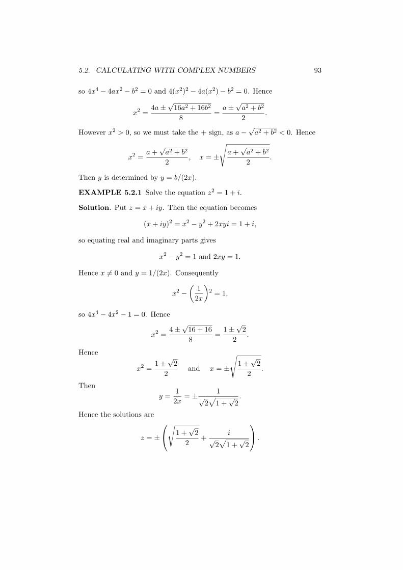
5.2. CALCULATING WITH COMPLEX NUMBERS 93
so 4x4 − 4ax2 − b2 = 0 and 4(x2)2 − 4a(x2) − b2 = 0. Hence
x2 =4a ±
√16a2 + 16b2
8=
a ±√
a2 + b2
2.
However x2 > 0, so we must take the + sign, as a −√
a2 + b2 < 0. Hence
x2 =a +
√a2 + b2
2, x = ±
√
a +√
a2 + b2
2.
Then y is determined by y = b/(2x).
EXAMPLE 5.2.1 Solve the equation z2 = 1 + i.
Solution. Put z = x + iy. Then the equation becomes
(x + iy)2 = x2 − y2 + 2xyi = 1 + i,
so equating real and imaginary parts gives
x2 − y2 = 1 and 2xy = 1.
Hence x 6= 0 and y = 1/(2x). Consequently
x2 −(
1
2x
)
2 = 1,
so 4x4 − 4x2 − 1 = 0. Hence
x2 =4 ±
√16 + 16
8=
1 ±√
2
2.
Hence
x2 =1 +
√2
2and x = ±
√
1 +√
2
2.
Then
y =1
2x= ± 1
√2√
1 +√
2.
Hence the solutions are
z = ±
√
1 +√
2
2+
i√
2√
1 +√
2
.
94 CHAPTER 5. COMPLEX NUMBERS
EXAMPLE 5.2.2 Solve the equation z2 + (√
3 + i)z + 1 = 0.
Solution. Because every complex number has a square root, the familiarformula
z =−b ±
√b2 − 4ac
2a
for the solution of the general quadratic equation az2 + bz + c = 0 can beused, where now a(6= 0), b, c ∈ C. Hence
z =−(
√3 + i) ±
√
(√
3 + i)2 − 4
2
=−(
√3 + i) ±
√
(3 + 2√
3i − 1) − 4
2
=−(
√3 + i) ±
√
−2 + 2√
3i
2.
Now we have to solve w2 = −2 + 2√
3i. Put w = x + iy. Then w2 =x2 − y2 + 2xyi = −2 + 2
√3i and equating real and imaginary parts gives
x2 − y2 = −2 and 2xy = 2√
3. Hence y =√
3/x and so x2 − 3/x2 = −2. Sox4 + 2x2 − 3 = 0 and (x2 + 3)(x2 − 1) = 0. Hence x2 − 1 = 0 and x = ±1.Then y = ±
√3. Hence (1 +
√3i)2 = −2 + 2
√3i and the formula for z now
becomes
z =−√
3 − i ± (1 +√
3i)
2
=1 −
√3 + (1 +
√3)i
2or
−1 −√
3 − (1 +√
3)i
2.
EXAMPLE 5.2.3 Find the cube roots of 1.
Solution. We have to solve the equation z3 = 1, or z3 − 1 = 0. Nowz3 − 1 = (z − 1)(z2 + z + 1). So z3 − 1 = 0 ⇒ z − 1 = 0 or z2 + z + 1 = 0.But
z2 + z + 1 = 0 ⇒ z =−1 ±
√12 − 4
2=
−1 ±√
3i
2.
So there are 3 cube roots of 1, namely 1 and (−1 ±√
3i)/2.
We state the next theorem without proof. It states that every non–constant polynomial with complex number coefficients has a root in thefield of complex numbers.
5.3. GEOMETRIC REPRESENTATION OF C 95
THEOREM 5.2.2 (Gauss) If f(z) = anzn + an−1zn−1 + · · · + a1z + a0,
where an 6= 0 and n ≥ 1, then f(z) = 0 for some z ∈ C.
It follows that in view of the factor theorem, which states that if a ∈ F isa root of a polynomial f(z) with coefficients from a field F , then z − a is afactor of f(z), that is f(z) = (z − a)g(z), where the coefficients of g(z) alsobelong to F . By repeated application of this result, we can factorize anypolynomial with complex coefficients into a product of linear factors withcomplex coefficients:
f(z) = an(z − z1)(z − z2) · · · (z − zn).
There are available a number of computational algorithms for finding goodapproximations to the roots of a polynomial with complex coefficients.
5.3 Geometric representation of C
Complex numbers can be represented as points in the plane, using the cor-respondence x + iy ↔ (x, y). The representation is known as the Argand
diagram or complex plane. The real complex numbers lie on the x–axis,which is then called the real axis, while the imaginary numbers lie on they–axis, which is known as the imaginary axis. The complex numbers withpositive imaginary part lie in the upper half plane, while those with negativeimaginary part lie in the lower half plane.
Because of the equation
(x1 + iy1) + (x2 + iy2) = (x1 + x2) + i(y1 + y2),
complex numbers add vectorially, using the parallellogram law. Similarly,the complex number z1 − z2 can be represented by the vector from (x2, y2)to (x1, y1), where z1 = x1 + iy1 and z2 = x2 + iy2. (See Figure 5.1.)
The geometrical representation of complex numbers can be very usefulwhen complex number methods are used to investigate properties of trianglesand circles. It is very important in the branch of calculus known as ComplexFunction theory, where geometric methods play an important role.
We mention that the line through two distinct points P1 = (x1, y1) andP2 = (x2, y2) has the form z = (1 − t)z1 + tz2, t ∈ R, where z = x + iy isany point on the line and zi = xi + iyi, i = 1, 2. For the line has parametricequations
x = (1 − t)x1 + tx2, y = (1 − t)y1 + ty2
and these can be combined into a single equation z = (1 − t)z1 + tz2.
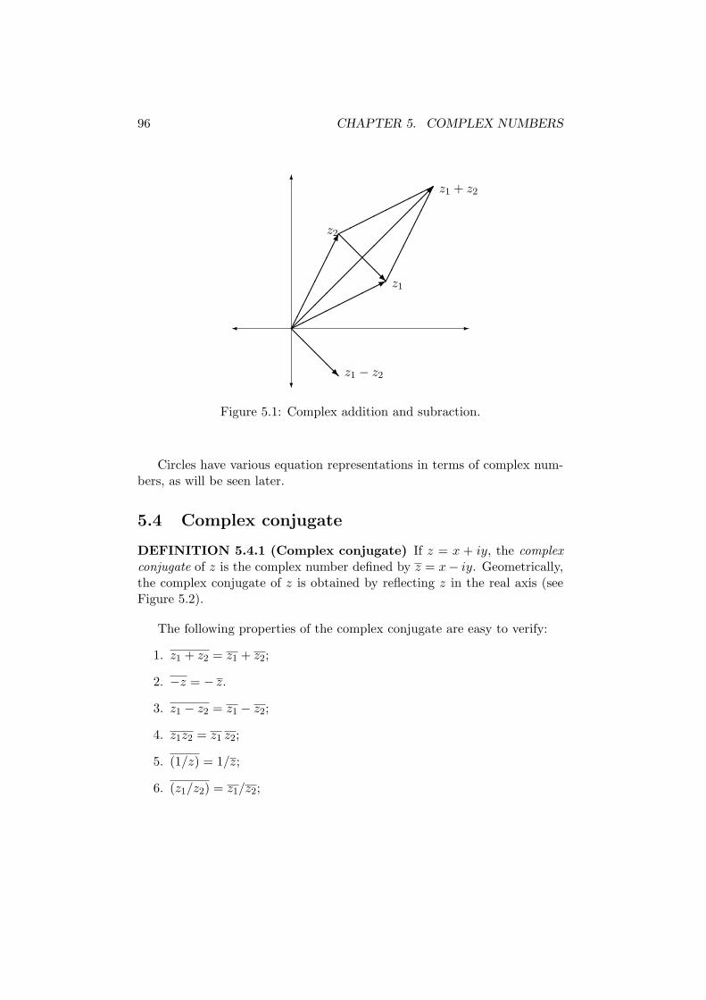
96 CHAPTER 5. COMPLEX NUMBERS
-¾
6
?z1 − z2
z1 + z2
z1
z2
¡¡
¡¡
¡¡
¡¡
¡¡
¡¡µ
©©©©©©©©*
¢¢¢¢¢¢¢¢
@@
@@R
@@
@@R
©©©©©©©©
¢¢¢¢¢¢¢¢
Figure 5.1: Complex addition and subraction.
Circles have various equation representations in terms of complex num-bers, as will be seen later.
5.4 Complex conjugate
DEFINITION 5.4.1 (Complex conjugate) If z = x + iy, the complex
conjugate of z is the complex number defined by z = x− iy. Geometrically,the complex conjugate of z is obtained by reflecting z in the real axis (seeFigure 5.2).
The following properties of the complex conjugate are easy to verify:
1. z1 + z2 = z1 + z2;
2. −z = − z.
3. z1 − z2 = z1 − z2;
4. z1z2 = z1 z2;
5. (1/z) = 1/z;
6. (z1/z2) = z1/z2;
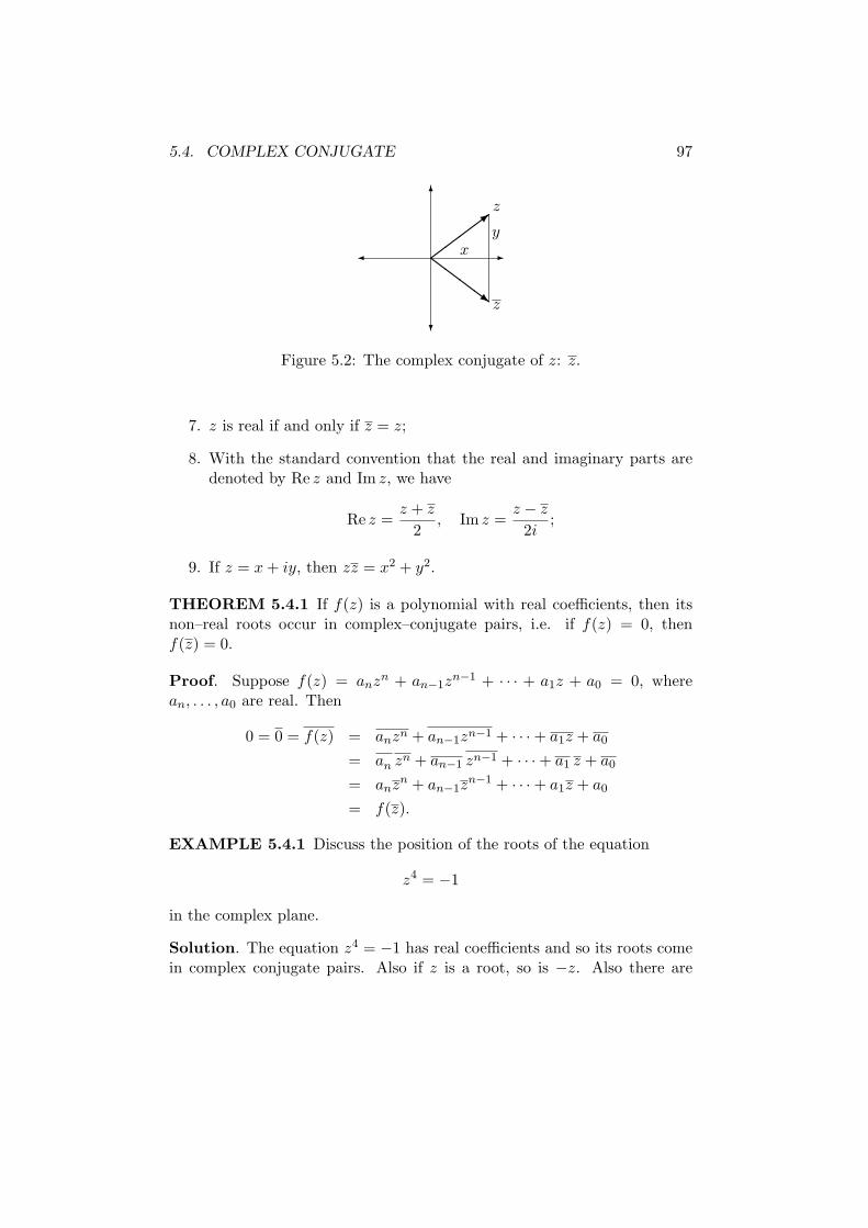
5.4. COMPLEX CONJUGATE 97
-¾
6
?
xy
z
z
½½
½½>
ZZ
ZZ~
Figure 5.2: The complex conjugate of z: z.
7. z is real if and only if z = z;
8. With the standard convention that the real and imaginary parts aredenoted by Re z and Im z, we have
Re z =z + z
2, Im z =
z − z
2i;
9. If z = x + iy, then zz = x2 + y2.
THEOREM 5.4.1 If f(z) is a polynomial with real coefficients, then itsnon–real roots occur in complex–conjugate pairs, i.e. if f(z) = 0, thenf(z) = 0.
Proof. Suppose f(z) = anzn + an−1zn−1 + · · · + a1z + a0 = 0, where
an, . . . , a0 are real. Then
0 = 0 = f(z) = anzn + an−1zn−1 + · · · + a1z + a0
= an zn + an−1 zn−1 + · · · + a1 z + a0
= anzn + an−1zn−1 + · · · + a1z + a0
= f(z).
EXAMPLE 5.4.1 Discuss the position of the roots of the equation
z4 = −1
in the complex plane.
Solution. The equation z4 = −1 has real coefficients and so its roots comein complex conjugate pairs. Also if z is a root, so is −z. Also there are
98 CHAPTER 5. COMPLEX NUMBERS
clearly no real roots and no imaginary roots. So there must be one root win the first quadrant, with all remaining roots being given by w, −w and−w. In fact, as we shall soon see, the roots lie evenly spaced on the unitcircle.
The following theorem is useful in deciding if a polynomial f(z) has amultiple root a; that is if (z − a)m divides f(z) for some m ≥ 2. (The proofis left as an exercise.)
THEOREM 5.4.2 If f(z) = (z − a)mg(z), where m ≥ 2 and g(z) is apolynomial, then f ′(a) = 0 and the polynomial and its derivative have acommon root.
From theorem 5.4.1 we obtain a result which is very useful in the explicitintegration of rational functions (i.e. ratios of polynomials) with real coeffi-cients.
THEOREM 5.4.3 If f(z) is a non–constant polynomial with real coeffi-cients, then f(z) can be factorized as a product of real linear factors andreal quadratic factors.
Proof. In general f(z) will have r real roots z1, . . . , zr and 2s non–realroots zr+1, zr+1, . . . , zr+s, zr+s, occurring in complex–conjugate pairs bytheorem 5.4.1. Then if an is the coefficient of highest degree in f(z), wehave the factorization
f(z) = an(z − z1) · · · (z − zr) ××(z − zr+1)(z − zr+1) · · · (z − zr+s)(z − zr+s).
We then use the following identity for j = r + 1, . . . , r + s which in turnshows that paired terms give rise to real quadratic factors:
(z − zj)(z − zj) = z2 − (zj + zj)z + zjzj
= z2 − 2Re zj + (x2j + y2
j ),
where zj = xj + iyj .
A well–known example of such a factorization is the following:
EXAMPLE 5.4.2 Factorize z4 + 1 into real linear and quadratic factors.
Solution. Clearly there are no real roots. Also we have the preliminaryfactorization z4 + 1 = (z2 − i)(z2 + i). Now the roots of z2 − i are easilyverified to be ±(1 + i)/
√2, so the roots of z2 + i must be ±(1 − i)/
√2.
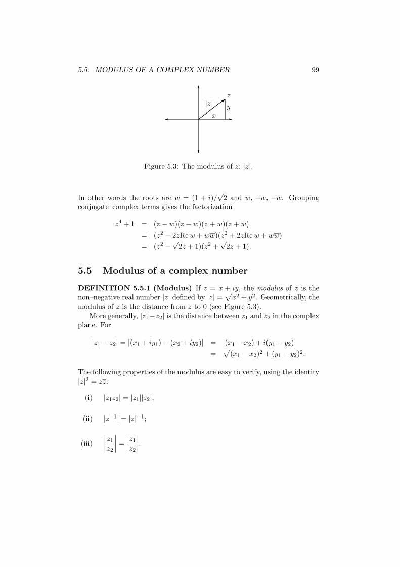
5.5. MODULUS OF A COMPLEX NUMBER 99
-¾
6
?
|z|x
y
z
½½
½½>
Figure 5.3: The modulus of z: |z|.
In other words the roots are w = (1 + i)/√
2 and w, −w, −w. Groupingconjugate–complex terms gives the factorization
z4 + 1 = (z − w)(z − w)(z + w)(z + w)
= (z2 − 2zRe w + ww)(z2 + 2zRe w + ww)
= (z2 −√
2z + 1)(z2 +√
2z + 1).
5.5 Modulus of a complex number
DEFINITION 5.5.1 (Modulus) If z = x + iy, the modulus of z is thenon–negative real number |z| defined by |z| =
√
x2 + y2. Geometrically, themodulus of z is the distance from z to 0 (see Figure 5.3).
More generally, |z1−z2| is the distance between z1 and z2 in the complexplane. For
|z1 − z2| = |(x1 + iy1) − (x2 + iy2)| = |(x1 − x2) + i(y1 − y2)|=
√
(x1 − x2)2 + (y1 − y2)2.
The following properties of the modulus are easy to verify, using the identity|z|2 = zz:
(i) |z1z2| = |z1||z2|;
(ii) |z−1| = |z|−1;
(iii)
∣
∣
∣
∣
z1
z2
∣
∣
∣
∣
=|z1||z2|
.
100 CHAPTER 5. COMPLEX NUMBERS
For example, to prove (i):
|z1z2|2 = (z1z2)z1z2 = (z1z2)z1 z2
= (z1z1)(z2z2) = |z1|2|z2|2 = (|z1||z2|)2.
Hence |z1z2| = |z1||z2|.
EXAMPLE 5.5.1 Find |z| when z =(1 + i)4
(1 + 6i)(2 − 7i).
Solution.
|z| =|1 + i|4
|1 + 6i||2 − 7i|
=(√
12 + 12)4√12 + 62
√
22 + (−7)2
=4√
37√
53.
THEOREM 5.5.1 (Ratio formulae) If z lies on the line through z1 andz2:
z = (1 − t)z1 + tz2, t ∈ R,
we have the useful ratio formulae:
(i)
∣
∣
∣
∣
z − z1
z − z2
∣
∣
∣
∣
=
∣
∣
∣
∣
t
1 − t
∣
∣
∣
∣
if z 6= z2,
(ii)
∣
∣
∣
∣
z − z1
z1 − z2
∣
∣
∣
∣
= |t|.
Circle equations. The equation |z − z0| = r, where z0 ∈ C and r >0, represents the circle centre z0 and radius r. For example the equation|z − (1 + 2i)| = 3 represents the circle (x − 1)2 + (y − 2)2 = 9.
Another useful circle equation is the circle of Apollonius :
∣
∣
∣
∣
z − a
z − b
∣
∣
∣
∣
= λ,
where a and b are distinct complex numbers and λ is a positive real number,λ 6= 1. (If λ = 1, the above equation represents the perpendicular bisectorof the segment joining a and b.)
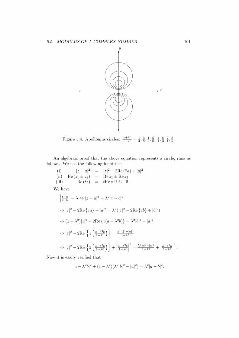
5.5. MODULUS OF A COMPLEX NUMBER 101
-¾
6
?
x
y
Figure 5.4: Apollonius circles: |z+2i||z−2i| = 1
4 , 38 , 1
2 , 58 ; 4
1 , 83 , 2
1 , 85 .
An algebraic proof that the above equation represents a circle, runs asfollows. We use the following identities:
(i) |z − a|2 = |z|2 − 2Re (za) + |a|2(ii) Re (z1 ± z2) = Re z1 ± Re z2
(iii) Re (tz) = tRe z if t ∈ R.
We have∣
∣
∣
z−az−b
∣
∣
∣ = λ ⇔ |z − a|2 = λ2|z − b|2
⇔ |z|2 − 2Re {za} + |a|2 = λ2(|z|2 − 2Re {zb} + |b|2)
⇔ (1 − λ2)|z|2 − 2Re {z(a − λ2b)} = λ2|b|2 − |a|2
⇔ |z|2 − 2Re{
z(
a−λ2b1−λ2
)}
= λ2|b|2−|a|21−λ2
⇔ |z|2 − 2Re{
z(
a−λ2b1−λ2
)}
+∣
∣
∣
a−λ2b1−λ2
∣
∣
∣
2= λ2|b|2−|a|2
1−λ2 +∣
∣
∣
a−λ2b1−λ2
∣
∣
∣
2.
Now it is easily verified that
|a − λ2b|2 + (1 − λ2)(λ2|b|2 − |a|2) = λ2|a − b|2.
102 CHAPTER 5. COMPLEX NUMBERS
So we obtain∣
∣
∣
∣
z − a
z − b
∣
∣
∣
∣
= λ ⇔∣
∣
∣
∣
z −(
a − λ2b
1 − λ2
)∣
∣
∣
∣
2
=λ2|a − b|2|1 − λ2|2
⇔∣
∣
∣
∣
z −(
a − λ2b
1 − λ2
)∣
∣
∣
∣
=λ|a − b||1 − λ2| .
The last equation represents a circle centre z0, radius r, where
z0 =a − λ2b
1 − λ2and r =
λ|a − b||1 − λ2| .
There are two special points on the circle of Apollonius, the points z1 andz2 defined by
z1 − a
z1 − b= λ and
z2 − a
z2 − b= −λ,
or
z1 =a − λb
1 − λand z2 =
a + λb
1 + λ. (5.3)
It is easy to verify that z1 and z2 are distinct points on the line through aand b and that z0 = z1+z2
2 . Hence the circle of Apollonius is the circle basedon the segment z1, z2 as diameter.
EXAMPLE 5.5.2 Find the centre and radius of the circle
|z − 1 − i| = 2|z − 5 − 2i|.Solution. Method 1. Proceed algebraically and simplify the equation
|x + iy − 1 − i| = 2|x + iy − 5 − 2i|
or|x − 1 + i(y − 1)| = 2|x − 5 + i(y − 2)|.
Squaring both sides gives
(x − 1)2 + (y − 1)2 = 4((x − 5)2 + (y − 2)2),
which reduces to the circle equation
x2 + y2 − 38
3x − 14
3y + 38 = 0.
Completing the square gives
(x − 19
3)2 + (y − 7
3)2 =
(
19
3
)2
+
(
7
3
)2
− 38 =68
9,
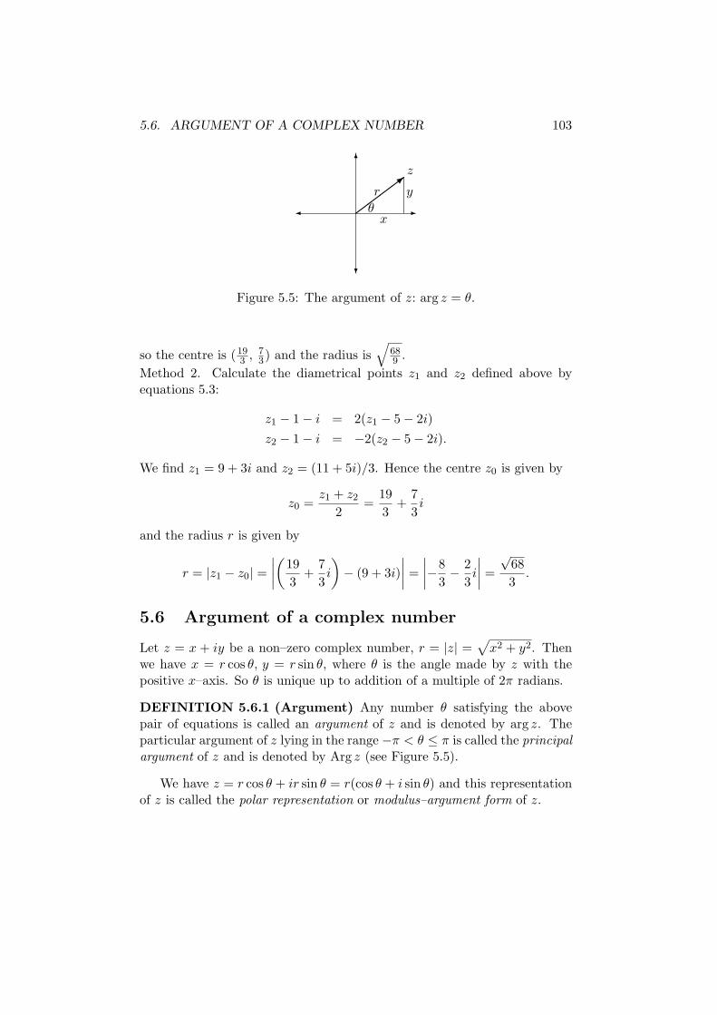
5.6. ARGUMENT OF A COMPLEX NUMBER 103
-¾
6
?
½½
½½>
x
yr
z
θ
Figure 5.5: The argument of z: arg z = θ.
so the centre is (193 , 7
3) and the radius is√
689 .
Method 2. Calculate the diametrical points z1 and z2 defined above byequations 5.3:
z1 − 1 − i = 2(z1 − 5 − 2i)
z2 − 1 − i = −2(z2 − 5 − 2i).
We find z1 = 9 + 3i and z2 = (11 + 5i)/3. Hence the centre z0 is given by
z0 =z1 + z2
2=
19
3+
7
3i
and the radius r is given by
r = |z1 − z0| =
∣
∣
∣
∣
(
19
3+
7
3i
)
− (9 + 3i)
∣
∣
∣
∣
=
∣
∣
∣
∣
−8
3− 2
3i
∣
∣
∣
∣
=
√68
3.
5.6 Argument of a complex number
Let z = x + iy be a non–zero complex number, r = |z| =√
x2 + y2. Thenwe have x = r cos θ, y = r sin θ, where θ is the angle made by z with thepositive x–axis. So θ is unique up to addition of a multiple of 2π radians.
DEFINITION 5.6.1 (Argument) Any number θ satisfying the abovepair of equations is called an argument of z and is denoted by arg z. Theparticular argument of z lying in the range −π < θ ≤ π is called the principal
argument of z and is denoted by Arg z (see Figure 5.5).
We have z = r cos θ + ir sin θ = r(cos θ + i sin θ) and this representationof z is called the polar representation or modulus–argument form of z.
104 CHAPTER 5. COMPLEX NUMBERS
EXAMPLE 5.6.1 Arg 1 = 0, Arg (−1) = π, Arg i = π2 , Arg (−i) = −π
2 .
We note that y/x = tan θ if x 6= 0, so θ is determined by this equation upto a multiple of π. In fact
Arg z = tan−1 y
x+ kπ,
where k = 0 if x > 0; k = 1 if x < 0, y > 0; k = −1 if x < 0, y < 0.
To determine Arg z graphically, it is simplest to draw the triangle formedby the points 0, x, z on the complex plane, mark in the positive acute angleα between the rays 0, x and 0, z and determine Arg z geometrically, usingthe fact that α = tan−1(|y|/|x|), as in the following examples:
EXAMPLE 5.6.2 Determine the principal argument of z for the followigcomplex numbers:
z = 4 + 3i, −4 + 3i, −4 − 3i, 4 − 3i.
Solution. Referring to Figure 5.6, we see that Arg z has the values
α, π − α, −π + α, −α,
where α = tan−1 34 .
An important property of the argument of a complex number states thatthe sum of the arguments of two non–zero complex numbers is an argumentof their product:
THEOREM 5.6.1 If θ1 and θ2 are arguments of z1 and z2, then θ1 + θ2
is an argument of z1z2.
Proof. Let z1 and z2 have polar representations z1 = r1(cos θ1 + i sin θ1)and z2 = r2(cos θ2 + i sin θ2). Then
z1z2 = r1(cos θ1 + i sin θ1)r2(cos θ2 + i sin θ2)
= r1r2(cos θ1 cos θ2 − sin θ1 sin θ2 + i(cos θ1 sin θ2 + sin θ1 cos θ2))
= r1r2(cos (θ1 + θ2) + i sin (θ1 + θ2)),
which is the polar representation of z1z2, as r1r2 = |z1||z2| = |z1z2|. Henceθ1 + θ2 is an argument of z1z2.
An easy induction gives the following generalization to a product of ncomplex numbers:
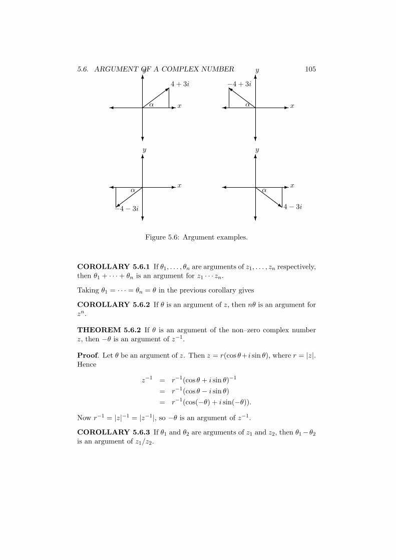
5.6. ARGUMENT OF A COMPLEX NUMBER 105
-¾
6
?
x
y
4 + 3i
α½½
½½>
-¾
6
?
x
y
−4 + 3i
αZZ
ZZ}
-¾
6
?
x
y
−4 − 3i
α½½
½½=
-¾
6
?
x
y
4 − 3i
αZZ
ZZ~
Figure 5.6: Argument examples.
COROLLARY 5.6.1 If θ1, . . . , θn are arguments of z1, . . . , zn respectively,then θ1 + · · · + θn is an argument for z1 · · · zn.
Taking θ1 = · · · = θn = θ in the previous corollary gives
COROLLARY 5.6.2 If θ is an argument of z, then nθ is an argument forzn.
THEOREM 5.6.2 If θ is an argument of the non–zero complex numberz, then −θ is an argument of z−1.
Proof. Let θ be an argument of z. Then z = r(cos θ+i sin θ), where r = |z|.Hence
z−1 = r−1(cos θ + i sin θ)−1
= r−1(cos θ − i sin θ)
= r−1(cos(−θ) + i sin(−θ)).
Now r−1 = |z|−1 = |z−1|, so −θ is an argument of z−1.
COROLLARY 5.6.3 If θ1 and θ2 are arguments of z1 and z2, then θ1−θ2
is an argument of z1/z2.
106 CHAPTER 5. COMPLEX NUMBERS
In terms of principal arguments, we have the following equations:
(i) Arg (z1z2) = Arg z1+Arg z2 + 2k1π,(ii) Arg (z−1) = −Arg z + 2k2π,(iii) Arg (z1/z2) = Arg z1−Arg z2 + 2k3π,(iv) Arg (z1 · · · zn) = Arg z1 + · · ·+Arg zn + 2k4π,(v) Arg (zn) = nArg z + 2k5π,
where k1, k2, k3, k4, k5 are integers.
In numerical examples, we can write (i), for example, as
Arg (z1z2) ≡ Arg z1 + Arg z2.
EXAMPLE 5.6.3 Find the modulus and principal argument of
z =
(√3 + i
1 + i
)17
and hence express z in modulus–argument form.
Solution. |z| =|√
3 + i|17|1 + i|17 =
217
(√
2)17= 217/2.
Arg z ≡ 17Arg
(√3 + i
1 + i
)
= 17(Arg (√
3 + i) − Arg (1 + i))
= 17(π
6− π
4
)
=−17π
12.
Hence Arg z =(−17π
12
)
+ 2kπ, where k is an integer. We see that k = 1 and
hence Arg z = 7π12 . Consequently z = 217/2
(
cos 7π12 + i sin 7π
12
)
.
DEFINITION 5.6.2 If θ is a real number, then we define eiθ by
eiθ = cos θ + i sin θ.
More generally, if z = x + iy, then we define ez by
ez = exeiy.
For example,
eiπ2 = i, eiπ = −1, e−
iπ2 = −i.
The following properties of the complex exponential function are left as
exercises:
5.7. DE MOIVRE’S THEOREM 107
THEOREM 5.6.3 (i) ez1ez2 = ez1+z2 ,(ii) ez1 · · · ezn = ez1+···+zn ,(iii) ez 6= 0,
(iv) (ez)−1 = e−z,(v) ez1/ez2 = ez1−z2 ,(vi) ez = ez.
THEOREM 5.6.4 The equation
ez = 1
has the complete solution z = 2kπi, k ∈Z.
Proof. First we observe that
e2kπi = cos (2kπ) + i sin (2kπ) = 1.
Conversely, suppose ez = 1, z = x + iy. Then ex(cos y + i sin y) = 1. Henceex cos y = 1 and ex sin y = 0. Hence sin y = 0 and so y = nπ, n ∈Z. Thenex cos (nπ) = 1, so ex(−1)n = 1, from which follows (−1)n = 1 as ex > 0.Hence n = 2k, k ∈Z and ex = 1. Hence x = 0 and z = 2kπi.
5.7 De Moivre’s theorem
The next theorem has many uses and is a special case of theorem 5.6.3(ii).Alternatively it can be proved directly by induction on n.
THEOREM 5.7.1 (De Moivre) If n is a positive integer, then
(cos θ + i sin θ)n = cos nθ + i sin nθ.
As a first application, we consider the equation zn = 1.
THEOREM 5.7.2 The equation zn = 1 has n distinct solutions, namely
the complex numbers ζk = e2kπi
n , k = 0, 1, . . . , n − 1. These lie equallyspaced on the unit circle |z| = 1 and are obtained by starting at 1, movinground the circle anti–clockwise, incrementing the argument in steps of 2π
n .(See Figure 5.7)
We notice that the roots are the powers of the special root ζ = e2πin .
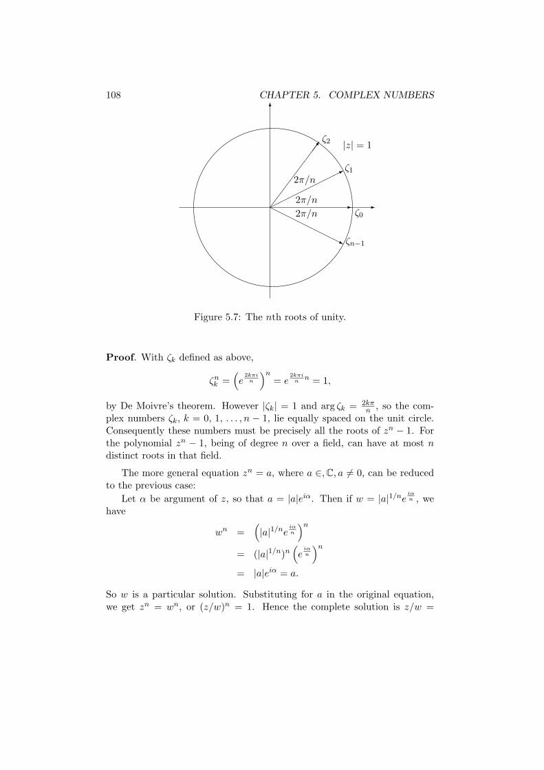
108 CHAPTER 5. COMPLEX NUMBERS
--ζ0
ζ1
ζ2
ζn−1
6
¶¶
¶¶
¶¶
¶¶7
©©©©©©©©*
HHHHHHHHj
2π/n
2π/n
2π/n
|z| = 1
Figure 5.7: The nth roots of unity.
Proof. With ζk defined as above,
ζnk =
(
e2kπi
n
)n= e
2kπin
n = 1,
by De Moivre’s theorem. However |ζk| = 1 and arg ζk = 2kπn , so the com-
plex numbers ζk, k = 0, 1, . . . , n − 1, lie equally spaced on the unit circle.Consequently these numbers must be precisely all the roots of zn − 1. Forthe polynomial zn − 1, being of degree n over a field, can have at most ndistinct roots in that field.
The more general equation zn = a, where a ∈, C, a 6= 0, can be reducedto the previous case:
Let α be argument of z, so that a = |a|eiα. Then if w = |a|1/neiαn , we
have
wn =(
|a|1/neiαn
)n
= (|a|1/n)n(
eiαn
)n
= |a|eiα = a.
So w is a particular solution. Substituting for a in the original equation,we get zn = wn, or (z/w)n = 1. Hence the complete solution is z/w =
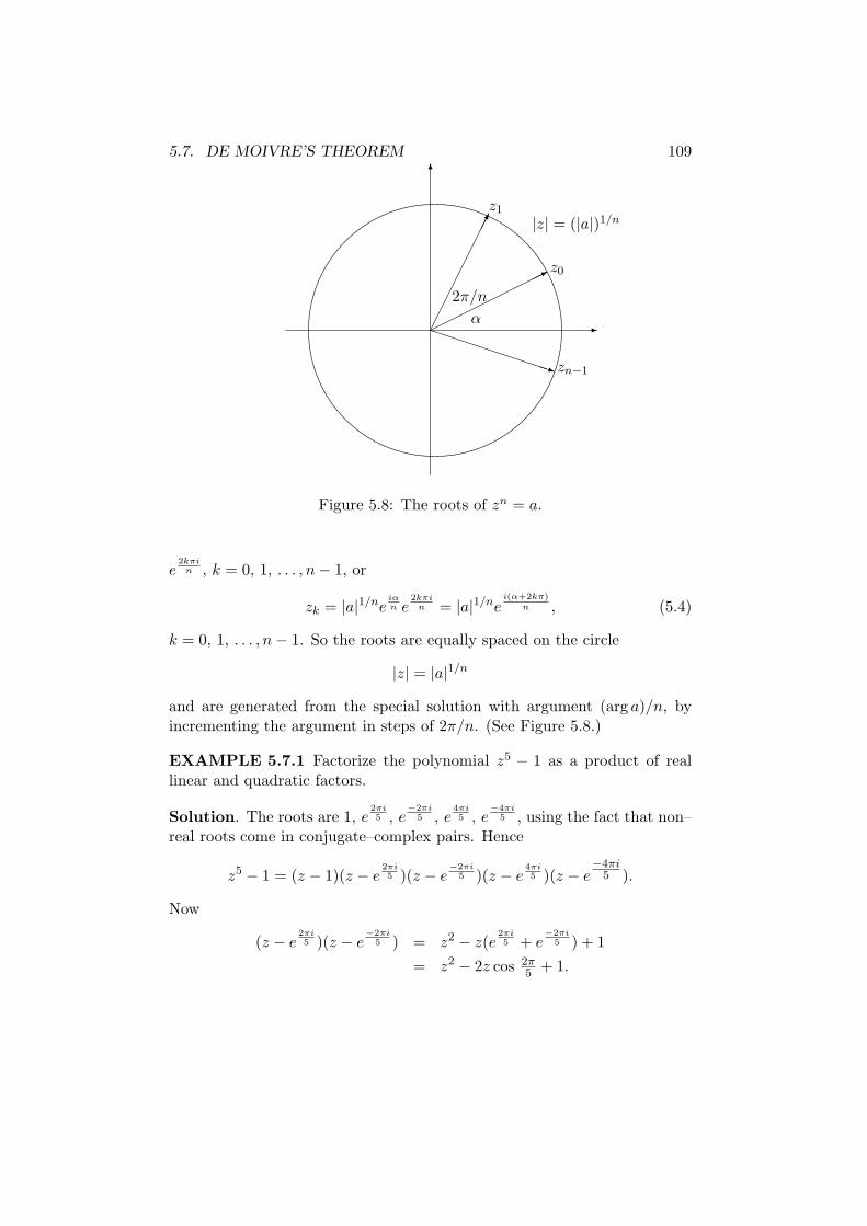
5.7. DE MOIVRE’S THEOREM 109
-
z0
z1
zn−1
6
PPPPPPPPPq
¢¢¢¢¢¢¢¢¢
©©©©©©©©©*
α
2π/n
|z| = (|a|)1/n
Figure 5.8: The roots of zn = a.
e2kπi
n , k = 0, 1, . . . , n − 1, or
zk = |a|1/neiαn e
2kπin = |a|1/ne
i(α+2kπ)n , (5.4)
k = 0, 1, . . . , n − 1. So the roots are equally spaced on the circle
|z| = |a|1/n
and are generated from the special solution with argument (arg a)/n, byincrementing the argument in steps of 2π/n. (See Figure 5.8.)
EXAMPLE 5.7.1 Factorize the polynomial z5 − 1 as a product of reallinear and quadratic factors.
Solution. The roots are 1, e2πi5 , e
−2πi5 , e
4πi5 , e
−4πi5 , using the fact that non–
real roots come in conjugate–complex pairs. Hence
z5 − 1 = (z − 1)(z − e2πi5 )(z − e
−2πi5 )(z − e
4πi5 )(z − e
−4πi5 ).
Now
(z − e2πi5 )(z − e
−2πi5 ) = z2 − z(e
2πi5 + e
−2πi5 ) + 1
= z2 − 2z cos 2π5 + 1.
110 CHAPTER 5. COMPLEX NUMBERS
Similarly
(z − e4πi5 )(z − e
−4πi5 ) = z2 − 2z cos 4π
5 + 1.
This gives the desired factorization.
EXAMPLE 5.7.2 Solve z3 = i.
Solution. |i| = 1 and Arg i = π2 = α. So by equation 5.4, the solutions are
zk = |i|1/3ei(α+2kπ)
3 , k = 0, 1, 2.
First, k = 0 gives
z0 = eiπ6 = cos
π
6+ i sin
π
6=
√3
2+
i
2.
Next, k = 1 gives
z1 = e5πi6 = cos
5π
6+ i sin
5π
6=
−√
3
2+
i
2.
Finally, k = 2 gives
z1 = e9πi6 = cos
9π
6+ i sin
9π
6= −i.
We finish this chapter with two more examples of De Moivre’s theorem.
EXAMPLE 5.7.3 If
C = 1 + cos θ + · · · + cos (n − 1)θ,
S = sin θ + · · · + sin (n − 1)θ,
prove that
C =sin nθ
2
sin θ2
cos (n−1)θ2 and S =
sin nθ2
sin θ2
sin (n−1)θ2 ,
if θ 6= 2kπ, k ∈Z.
5.8. PROBLEMS 111
Solution.
C + iS = 1 + (cos θ + i sin θ) + · · · + (cos (n − 1)θ + i sin (n − 1)θ)
= 1 + eiθ + · · · + ei(n−1)θ
= 1 + z + · · · + zn−1, where z = eiθ
=1 − zn
1 − z, if z 6= 1, i.e. θ 6= 2kπ,
=1 − einθ
1 − eiθ=
einθ2 (e
−inθ2 − e
inθ2 )
eiθ2 (e
−iθ2 − e
iθ2 )
= ei(n−1) θ2sin nθ
2
sin θ2
= (cos (n − 1) θ2 + i sin (n − 1) θ
2)sin nθ
2
sin θ2
.
The result follows by equating real and imaginary parts.
EXAMPLE 5.7.4 Express cos nθ and sin nθ in terms of cos θ and sin θ,using the equation cos nθ + sin nθ = (cos θ + i sin θ)n.
Solution. The binomial theorem gives
(cos θ + i sin θ)n = cosn θ +(
n1
)
cosn−1 θ(i sin θ) +(
n2
)
cosn−2 θ(i sin θ)2 + · · ·+ (i sin θ)n.
Equating real and imaginary parts gives
cos nθ = cosn θ −(
n2
)
cosn−2 θ sin2 θ + · · ·sin nθ =
(
n1
)
cosn−1 θ sin θ −(
n3
)
cosn−3 θ sin3 θ + · · · .
5.8 PROBLEMS
1. Express the following complex numbers in the form x + iy, x, y real:
(i) (−3 + i)(14 − 2i); (ii)2 + 3i
1 − 4i; (iii)
(1 + 2i)2
1 − i.
[Answers: (i) −40 + 20i; (ii) −1017 + 11
17 i; (iii) −72 + i
2 .]
2. Solve the following equations:
112 CHAPTER 5. COMPLEX NUMBERS
(i) iz + (2 − 10i)z = 3z + 2i,
(ii) (1 + i)z + (2 − i)w = −3i(1 + 2i)z + (3 + i)w = 2 + 2i.
[Answers:(i) z = − 941 − i
41 ; (ii) z = −1 + 5i, w = 195 − 8i
5 .]
3. Express 1 + (1 + i) + (1 + i)2 + . . . + (1 + i)99 in the form x + iy, x, yreal. [Answer: (1 + 250)i.]
4. Solve the equations: (i) z2 = −8− 6i; (ii) z2 − (3 + i)z + 4 + 3i = 0.
[Answers: (i) z = ±(1 − 3i); (ii) z = 2 − i, 1 + 2i.]
5. Find the modulus and principal argument of each of the followingcomplex numbers:
(i) 4 + i; (ii) −32 − i
2 ; (iii) −1 + 2i; (iv) 12(−1 + i
√3).
[Answers: (i)√
17, tan−1 14 ; (ii)
√102 , −π + tan−1 1
3 ; (iii)√
5, π −tan−1 2.]
6. Express the following complex numbers in modulus-argument form:
(i) z = (1 + i)(1 + i√
3)(√
3 − i).
(ii) z =(1 + i)5(1 − i
√3)5
(√
3 + i)4.
[Answers:
(i) z = 4√
2(cos 5π12 + i sin 5π
12 ); (ii) z = 27/2(cos 11π12 + i sin 11π
12 ).]
7. (i) If z = 2(cos π4 +i sin π
4 ) and w = 3(cos π6 +i sin π
6 ), find the polarform of
(a) zw; (b) zw ; (c) w
z ; (d) z5
w2 .
(ii) Express the following complex numbers in the form x + iy:
(a) (1 + i)12; (b)(
1−i√2
)−6.
[Answers: (i): (a) 6(cos 5π12 + i sin 5π
12 ); (b) 23(cos π
12 + i sin π12);
(c) 32(cos − π
12 + i sin − π12); (d) 32
9 (cos 11π12 + i sin 11π
12 );
(ii): (a) −64; (b) −i.]
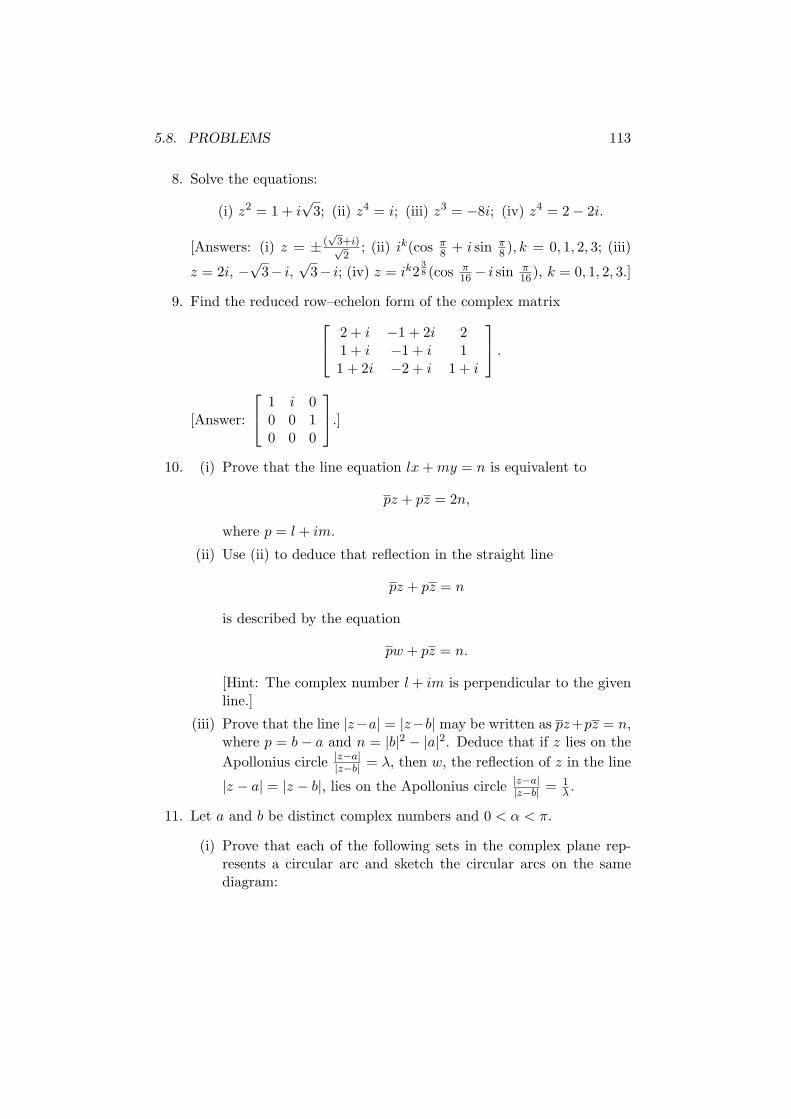
5.8. PROBLEMS 113
8. Solve the equations:
(i) z2 = 1 + i√
3; (ii) z4 = i; (iii) z3 = −8i; (iv) z4 = 2 − 2i.
[Answers: (i) z = ± (√
3+i)√2
; (ii) ik(cos π8 + i sin π
8 ), k = 0, 1, 2, 3; (iii)
z = 2i, −√
3− i,√
3− i; (iv) z = ik238 (cos π
16 − i sin π16), k = 0, 1, 2, 3.]
9. Find the reduced row–echelon form of the complex matrix
2 + i −1 + 2i 21 + i −1 + i 11 + 2i −2 + i 1 + i
.
[Answer:
1 i 00 0 10 0 0
.]
10. (i) Prove that the line equation lx + my = n is equivalent to
pz + pz = 2n,
where p = l + im.
(ii) Use (ii) to deduce that reflection in the straight line
pz + pz = n
is described by the equation
pw + pz = n.
[Hint: The complex number l + im is perpendicular to the givenline.]
(iii) Prove that the line |z−a| = |z−b| may be written as pz+pz = n,where p = b − a and n = |b|2 − |a|2. Deduce that if z lies on the
Apollonius circle |z−a||z−b| = λ, then w, the reflection of z in the line
|z − a| = |z − b|, lies on the Apollonius circle |z−a||z−b| = 1
λ .
11. Let a and b be distinct complex numbers and 0 < α < π.
(i) Prove that each of the following sets in the complex plane rep-resents a circular arc and sketch the circular arcs on the samediagram:
114 CHAPTER 5. COMPLEX NUMBERS
Argz − a
z − b= α, −α, π − α, α − π.
Also show that Argz − a
z − b= π represents the line segment joining
a and b, while Argz − a
z − b= 0 represents the remaining portion of
the line through a and b.
(ii) Use (i) to prove that four distinct points z1, z2, z3, z4 are con-cyclic or collinear, if and only if the cross–ratio
z4 − z1
z4 − z2/z3 − z1
z3 − z2
is real.
(iii) Use (ii) to derive Ptolemy’s Theorem: Distinct points A, B, C, Dare concyclic or collinear, if and only if one of the following holds:
AB · CD + BC · AD = AC · BD
BD · AC + AD · BC = AB · CD
BD · AC + AB · CD = AD · BC.
Chapter 6
EIGENVALUES AND
EIGENVECTORS
6.1 Motivation
We motivate the chapter on eigenvalues by discussing the equation
ax2 + 2hxy + by2 = c,
where not all of a, h, b are zero. The expression ax2 + 2hxy + by2 is calleda quadratic form in x and y and we have the identity
ax2 + 2hxy + by2 =[
x y]
[
a hh b
] [
xy
]
= XtAX,
where X =
[
xy
]
and A =
[
a hh b
]
. A is called the matrix of the quadratic
form.
We now rotate the x, y axes anticlockwise through θ radians to newx1, y1 axes. The equations describing the rotation of axes are derived asfollows:
Let P have coordinates (x, y) relative to the x, y axes and coordinates(x1, y1) relative to the x1, y1 axes. Then referring to Figure 6.1:
115
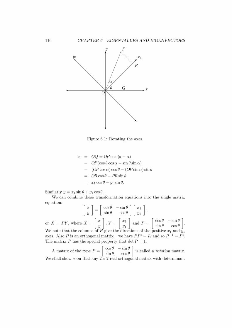
116 CHAPTER 6. EIGENVALUES AND EIGENVECTORS
-¾
6
?
¡¡
¡¡
¡¡
¡¡µ
@@
@@
@@
@@I
¡¡
¡¡
¡¡
¡¡µ
@@
@@
@@
@@R
¯¯¯¯¯¯¯¯¯¯@
@@
x
y
x1y1
P
Q
R
O
α
θ
Figure 6.1: Rotating the axes.
x = OQ = OP cos (θ + α)
= OP (cos θ cos α − sin θ sinα)
= (OP cos α) cos θ − (OP sinα) sin θ
= OR cos θ − PR sin θ
= x1 cos θ − y1 sin θ.
Similarly y = x1 sin θ + y1 cos θ.We can combine these transformation equations into the single matrix
equation:[
xy
]
=
[
cos θ − sin θsin θ cos θ
] [
x1
y1
]
,
or X = PY , where X =
[
xy
]
, Y =
[
x1
y1
]
and P =
[
cos θ − sin θsin θ cos θ
]
.
We note that the columns of P give the directions of the positive x1 and y1
axes. Also P is an orthogonal matrix – we have PP t = I2 and so P−1 = P t.The matrix P has the special property that detP = 1.
A matrix of the type P =
[
cos θ − sin θsin θ cos θ
]
is called a rotation matrix.
We shall show soon that any 2× 2 real orthogonal matrix with determinant
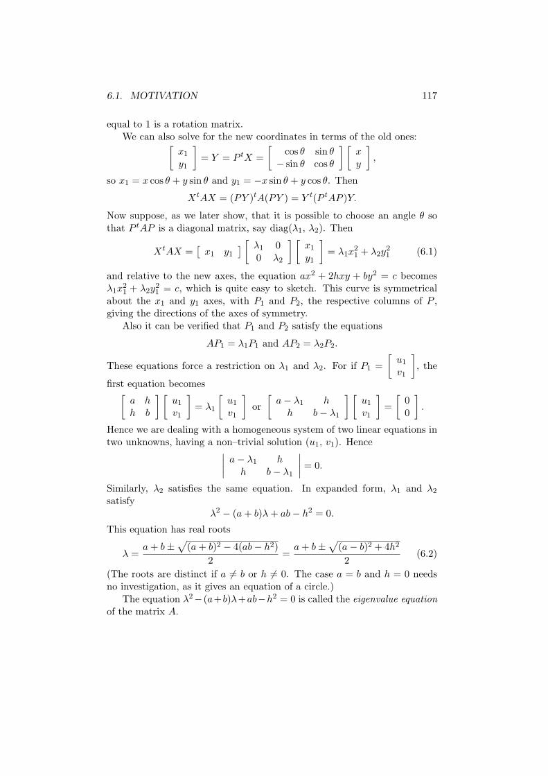
6.1. MOTIVATION 117
equal to 1 is a rotation matrix.We can also solve for the new coordinates in terms of the old ones:
[
x1
y1
]
= Y = P tX =
[
cos θ sin θ− sin θ cos θ
] [
xy
]
,
so x1 = x cos θ + y sin θ and y1 = −x sin θ + y cos θ. Then
XtAX = (PY )tA(PY ) = Y t(P tAP )Y.
Now suppose, as we later show, that it is possible to choose an angle θ sothat P tAP is a diagonal matrix, say diag(λ1, λ2). Then
XtAX =[
x1 y1
]
[
λ1 00 λ2
] [
x1
y1
]
= λ1x21 + λ2y
21 (6.1)
and relative to the new axes, the equation ax2 + 2hxy + by2 = c becomesλ1x
21 + λ2y
21 = c, which is quite easy to sketch. This curve is symmetrical
about the x1 and y1 axes, with P1 and P2, the respective columns of P ,giving the directions of the axes of symmetry.
Also it can be verified that P1 and P2 satisfy the equations
AP1 = λ1P1 and AP2 = λ2P2.
These equations force a restriction on λ1 and λ2. For if P1 =
[
u1
v1
]
, the
first equation becomes[
a hh b
] [
u1
v1
]
= λ1
[
u1
v1
]
or
[
a − λ1 hh b − λ1
] [
u1
v1
]
=
[
00
]
.
Hence we are dealing with a homogeneous system of two linear equations intwo unknowns, having a non–trivial solution (u1, v1). Hence
∣
∣
∣
∣
a − λ1 hh b − λ1
∣
∣
∣
∣
= 0.
Similarly, λ2 satisfies the same equation. In expanded form, λ1 and λ2
satisfyλ2 − (a + b)λ + ab − h2 = 0.
This equation has real roots
λ =a + b ±
√
(a + b)2 − 4(ab − h2)
2=
a + b ±√
(a − b)2 + 4h2
2(6.2)
(The roots are distinct if a 6= b or h 6= 0. The case a = b and h = 0 needsno investigation, as it gives an equation of a circle.)
The equation λ2− (a+b)λ+ab−h2 = 0 is called the eigenvalue equation
of the matrix A.
118 CHAPTER 6. EIGENVALUES AND EIGENVECTORS
6.2 Definitions and examples
DEFINITION 6.2.1 (Eigenvalue, eigenvector) Let A be a complexsquare matrix. Then if λ is a complex number and X a non–zero com-plex column vector satisfying AX = λX, we call X an eigenvector of A,while λ is called an eigenvalue of A. We also say that X is an eigenvectorcorresponding to the eigenvalue λ.
So in the above example P1 and P2 are eigenvectors corresponding to λ1
and λ2, respectively. We shall give an algorithm which starts from the
eigenvalues of A =
[
a hh b
]
and constructs a rotation matrix P such that
P tAP is diagonal.
As noted above, if λ is an eigenvalue of an n × n matrix A, withcorresponding eigenvector X, then (A − λIn)X = 0, with X 6= 0, sodet (A − λIn) = 0 and there are at most n distinct eigenvalues of A.
Conversely if det (A − λIn) = 0, then (A − λIn)X = 0 has a non–trivialsolution X and so λ is an eigenvalue of A with X a corresponding eigenvector.
DEFINITION 6.2.2 (Characteristic polynomial, equation)The polynomial det (A − λIn) is called the characteristic polynomial of Aand is often denoted by chA(λ). The equation det (A − λIn) = 0 is calledthe characteristic equation of A. Hence the eigenvalues of A are the rootsof the characteristic polynomial of A.
For a 2× 2 matrix A =
[
a bc d
]
, it is easily verified that the character-
istic polynomial is λ2 − (traceA)λ+det A, where trace A = a+d is the sumof the diagonal elements of A.
EXAMPLE 6.2.1 Find the eigenvalues of A =
[
2 11 2
]
and find all eigen-
vectors.
Solution. The characteristic equation of A is λ2 − 4λ + 3 = 0, or
(λ − 1)(λ − 3) = 0.
Hence λ = 1 or 3. The eigenvector equation (A − λIn)X = 0 reduces to
[
2 − λ 11 2 − λ
] [
xy
]
=
[
00
]
,
6.2. DEFINITIONS AND EXAMPLES 119
or
(2 − λ)x + y = 0
x + (2 − λ)y = 0.
Taking λ = 1 gives
x + y = 0
x + y = 0,
which has solution x = −y, y arbitrary. Consequently the eigenvectors
corresponding to λ = 1 are the vectors
[
−yy
]
, with y 6= 0.
Taking λ = 3 gives
−x + y = 0
x − y = 0,
which has solution x = y, y arbitrary. Consequently the eigenvectors corre-
sponding to λ = 3 are the vectors
[
yy
]
, with y 6= 0.
Our next result has wide applicability:
THEOREM 6.2.1 Let A be a 2× 2 matrix having distinct eigenvalues λ1
and λ2 and corresponding eigenvectors X1 and X2. Let P be the matrixwhose columns are X1 and X2, respectively. Then P is non–singular and
P−1AP =
[
λ1 00 λ2
]
.
Proof. Suppose AX1 = λ1X1 and AX2 = λ2X2. We show that the systemof homogeneous equations
xX1 + yX2 = 0
has only the trivial solution. Then by theorem 2.5.10 the matrix P =[X1|X2] is non–singular. So assume
xX1 + yX2 = 0. (6.3)
Then A(xX1 + yX2) = A0 = 0, so x(AX1) + y(AX2) = 0. Hence
xλ1X1 + yλ2X2 = 0. (6.4)
120 CHAPTER 6. EIGENVALUES AND EIGENVECTORS
Multiplying equation 6.3 by λ1 and subtracting from equation 6.4 gives
(λ2 − λ1)yX2 = 0.
Hence y = 0, as (λ2−λ1) 6= 0 and X2 6= 0. Then from equation 6.3, xX1 = 0and hence x = 0.
Then the equations AX1 = λ1X1 and AX2 = λ2X2 give
AP = A[X1|X2] = [AX1|AX2] = [λ1X1|λ2X2]
= [X1|X2]
[
λ1 00 λ2
]
= P
[
λ1 00 λ2
]
,
so
P−1AP =
[
λ1 00 λ2
]
.
EXAMPLE 6.2.2 Let A =
[
2 11 2
]
be the matrix of example 6.2.1. Then
X1 =
[
−11
]
and X2 =
[
11
]
are eigenvectors corresponding to eigenvalues
1 and 3, respectively. Hence if P =
[
−1 11 1
]
, we have
P−1AP =
[
1 00 3
]
.
There are two immediate applications of theorem 6.2.1. The first is to thecalculation of An: If P−1AP = diag (λ1, λ2), then A = Pdiag (λ1, λ2)P
−1
and
An =
(
P
[
λ1 00 λ2
]
P−1
)n
= P
[
λ1 00 λ2
]n
P−1 = P
[
λn1 00 λn
2
]
P−1.
The second application is to solving a system of linear differential equations
dx
dt= ax + by
dy
dt= cx + dy,
where A =
[
a bc d
]
is a matrix of real or complex numbers and x and y
are functions of t. The system can be written in matrix form as X = AX,where
X =
[
xy
]
and X =
[
xy
]
=
[ dxdtdydt
]
.
6.2. DEFINITIONS AND EXAMPLES 121
We make the substitution X = PY , where Y =
[
x1
y1
]
. Then x1 and y1
are also functions of t and
X = PY = AX = A(PY ), so Y = (P−1AP )Y =
[
λ1 00 λ2
]
Y.
Hence x1 = λ1x1 and y1 = λ2y1.These differential equations are well–known to have the solutions x1 =
x1(0)eλ1t and y1 = y1(0)eλ2t, where x1(0) is the value of x1 when t = 0.
[If dxdt = kx, where k is a constant, then
d
dt
(
e−ktx)
= −ke−ktx + e−kt dx
dt= −ke−ktx + e−ktkx = 0.
Hence e−ktx is constant, so e−ktx = e−k0x(0) = x(0). Hence x = x(0)ekt.]
However
[
x1(0)y1(0)
]
= P−1
[
x(0)y(0)
]
, so this determines x1(0) and y1(0) in
terms of x(0) and y(0). Hence ultimately x and y are determined as explicitfunctions of t, using the equation X = PY .
EXAMPLE 6.2.3 Let A =
[
2 −34 −5
]
. Use the eigenvalue method to
derive an explicit formula for An and also solve the system of differentialequations
dx
dt= 2x − 3y
dy
dt= 4x − 5y,
given x = 7 and y = 13 when t = 0.
Solution. The characteristic polynomial of A is λ2+3λ+2 which has distinct
roots λ1 = −1 and λ2 = −2. We find corresponding eigenvectors X1 =
[
11
]
and X2 =
[
34
]
. Hence if P =
[
1 31 4
]
, we have P−1AP = diag (−1, −2).
Hence
An =(
Pdiag (−1, −2)P−1)n
= Pdiag ((−1)n, (−2)n)P−1
=
[
1 31 4
] [
(−1)n 00 (−2)n
] [
4 −3−1 1
]
122 CHAPTER 6. EIGENVALUES AND EIGENVECTORS
= (−1)n
[
1 31 4
] [
1 00 2n
] [
4 −3−1 1
]
= (−1)n
[
1 3 × 2n
1 4 × 2n
] [
4 −3−1 1
]
= (−1)n
[
4 − 3 × 2n −3 + 3 × 2n
4 − 4 × 2n −3 + 4 × 2n
]
.
To solve the differential equation system, make the substitution X =PY . Then x = x1 + 3y1, y = x1 + 4y1. The system then becomes
x1 = −x1
y1 = −2y1,
so x1 = x1(0)e−t, y1 = y1(0)e−2t. Now
[
x1(0)y1(0)
]
= P−1
[
x(0)y(0)
]
=
[
4 −3−1 1
] [
713
]
=
[
−116
]
,
so x1 = −11e−t and y1 = 6e−2t. Hence x = −11e−t + 3(6e−2t) = −11e−t +18e−2t, y = −11e−t + 4(6e−2t) = −11e−t + 24e−2t.
For a more complicated example we solve a system of inhomogeneous
recurrence relations.
EXAMPLE 6.2.4 Solve the system of recurrence relations
xn+1 = 2xn − yn − 1
yn+1 = −xn + 2yn + 2,
given that x0 = 0 and y0 = −1.
Solution. The system can be written in matrix form as
Xn+1 = AXn + B,
where
A =
[
2 −1−1 2
]
and B =
[
−12
]
.
It is then an easy induction to prove that
Xn = AnX0 + (An−1 + · · · + A + I2)B. (6.5)
6.2. DEFINITIONS AND EXAMPLES 123
Also it is easy to verify by the eigenvalue method that
An =1
2
[
1 + 3n 1 − 3n
1 − 3n 1 + 3n
]
=1
2U +
3n
2V,
where U =
[
1 11 1
]
and V =
[
1 −1−1 1
]
. Hence
An−1 + · · · + A + I2 =n
2U +
(3n−1 + · · · + 3 + 1)
2V
=n
2U +
(3n−1 − 1)
4V.
Then equation 6.5 gives
Xn =
(
1
2U +
3n
2V
) [
0−1
]
+
(
n
2U +
(3n−1 − 1)
4V
) [
−12
]
,
which simplifies to[
xn
yn
]
=
[
(2n + 1 − 3n)/4(2n − 5 + 3n)/4
]
.
Hence xn = (2n − 1 + 3n)/4 and yn = (2n − 5 + 3n)/4.
REMARK 6.2.1 If (A − I2)−1 existed (that is, if det (A − I2) 6= 0, or
equivalently, if 1 is not an eigenvalue of A), then we could have used theformula
An−1 + · · · + A + I2 = (An − I2)(A − I2)−1. (6.6)
However the eigenvalues of A are 1 and 3 in the above problem, so formula 6.6cannot be used there.
Our discussion of eigenvalues and eigenvectors has been limited to 2 × 2matrices. The discussion is more complicated for matrices of size greaterthan two and is best left to a second course in linear algebra. Neverthelessthe following result is a useful generalization of theorem 6.2.1. The readeris referred to [28, page 350] for a proof.
THEOREM 6.2.2 Let A be an n × n matrix having distinct eigenvaluesλ1, . . . , λn and corresponding eigenvectors X1, . . . , Xn. Let P be the matrixwhose columns are respectively X1, . . . , Xn. Then P is non–singular and
P−1AP =
λ1 0 · · · 00 λ2 · · · 0...
......
...0 0 · · · λn
.
124 CHAPTER 6. EIGENVALUES AND EIGENVECTORS
Another useful result which covers the case where there are multiple eigen-values is the following (The reader is referred to [28, pages 351–352] for aproof):
THEOREM 6.2.3 Suppose the characteristic polynomial of A has the fac-torization
det (λIn − A) = (λ − c1)n1 · · · (λ − ct)
nt ,
where c1, . . . , ct are the distinct eigenvalues of A. Suppose that for i =1, . . . , t, we have nullity (ciIn − A) = ni. For each such i, choose a basisXi1, . . . , Xini
for the eigenspace N(ciIn − A). Then the matrix
P = [X11| · · · |X1n1 | · · · |Xt1| · · · |Xtnt ]
is non–singular and P−1AP is the following diagonal matrix
P−1AP =
c1In1 0 · · · 00 c2In2 · · · 0...
......
...0 0 · · · ctInt
.
(The notation means that on the diagonal there are n1 elements c1, followedby n2 elements c2,. . . , nt elements ct.)
6.3 PROBLEMS
1. Let A =
[
4 −31 0
]
. Find an invertible matrix P such that P−1AP =
diag (1, 3) and hence prove that
An =3n − 1
2A +
3 − 3n
2I2.
2. If A =
[
0.6 0.80.4 0.2
]
, prove that An tends to a limiting matrix
[
2/3 2/31/3 1/3
]
as n → ∞.
6.3. PROBLEMS 125
3. Solve the system of differential equations
dx
dt= 3x − 2y
dy
dt= 5x − 4y,
given x = 13 and y = 22 when t = 0.
[Answer: x = 7et + 6e−2t, y = 7et + 15e−2t.]
4. Solve the system of recurrence relations
xn+1 = 3xn − yn
yn+1 = −xn + 3yn,
given that x0 = 1 and y0 = 2.
[Answer: xn = 2n−1(3 − 2n), yn = 2n−1(3 + 2n).]
5. Let A =
[
a bc d
]
be a real or complex matrix with distinct eigenvalues
λ1, λ2 and corresponding eigenvectors X1, X2. Also let P = [X1|X2].
(a) Prove that the system of recurrence relations
xn+1 = axn + byn
yn+1 = cxn + dyn
has the solution[
xn
yn
]
= αλn1X1 + βλn
2X2,
where α and β are determined by the equation[
αβ
]
= P−1
[
x0
y0
]
.
(b) Prove that the system of differential equations
dx
dt= ax + by
dy
dt= cx + dy
has the solution[
xy
]
= αeλ1tX1 + βeλ2tX2,
126 CHAPTER 6. EIGENVALUES AND EIGENVECTORS
where α and β are determined by the equation
[
αβ
]
= P−1
[
x(0)y(0)
]
.
6. Let A =
[
a11 a12
a21 a22
]
be a real matrix with non–real eigenvalues λ =
a + ib and λ = a − ib, with corresponding eigenvectors X = U + iVand X = U − iV , where U and V are real vectors. Also let P be thereal matrix defined by P = [U |V ]. Finally let a + ib = reiθ, wherer > 0 and θ is real.
(a) Prove that
AU = aU − bV
AV = bU + aV.
(b) Deduce that
P−1AP =
[
a b−b a
]
.
(c) Prove that the system of recurrence relations
xn+1 = a11xn + a12yn
yn+1 = a21xn + a22yn
has the solution[
xn
yn
]
= rn{(αU + βV ) cos nθ + (βU − αV ) sinnθ},
where α and β are determined by the equation
[
αβ
]
= P−1
[
x0
y0
]
.
(d) Prove that the system of differential equations
dx
dt= ax + by
dy
dt= cx + dy
6.3. PROBLEMS 127
has the solution[
xy
]
= eat{(αU + βV ) cos bt + (βU − αV ) sin bt},
where α and β are determined by the equation[
αβ
]
= P−1
[
x(0)y(0)
]
.
[Hint: Let
[
xy
]
= P
[
x1
y1
]
. Also let z = x1 + iy1. Prove that
z = (a − ib)z
and deduce that
x1 + iy1 = eat(α + iβ)(cos bt + i sin bt).
Then equate real and imaginary parts to solve for x1, y1 andhence x, y.]
7. (The case of repeated eigenvalues.) Let A =
[
a bc d
]
and suppose
that the characteristic polynomial of A, λ2 − (a + d)λ + (ad− bc), hasa repeated root α. Also assume that A 6= αI2. Let B = A − αI2.
(i) Prove that (a − d)2 + 4bc = 0.
(ii) Prove that B2 = 0.
(iii) Prove that BX2 6= 0 for some vector X2; indeed, show that X2
can be taken to be
[
10
]
or
[
01
]
.
(iv) Let X1 = BX2. Prove that P = [X1|X2] is non–singular,
AX1 = αX1 and AX2 = αX2 + X1
and deduce that
P−1AP =
[
α 10 α
]
.
8. Use the previous result to solve system of the differential equations
dx
dt= 4x − y
dy
dt= 4x + 8y,
128 CHAPTER 6. EIGENVALUES AND EIGENVECTORS
given that x = 1 = y when t = 0.
[To solve the differential equation
dx
dt− kx = f(t), k a constant,
multiply throughout by e−kt, thereby converting the left–hand side todxdt (e
−ktx).]
[Answer: x = (1 − 3t)e6t, y = (1 + 6t)e6t.]
9. Let
A =
1/2 1/2 01/4 1/4 1/21/4 1/4 1/2
.
(a) Verify that det (λI3 − A), the characteristic polynomial of A, isgiven by
(λ − 1)λ(λ − 1
4).
(b) Find a non–singular matrix P such that P−1AP = diag (1, 0, 14).
(c) Prove that
An =1
3
1 1 11 1 11 1 1
+1
3 · 4n
2 2 −4−1 −1 2−1 −1 2
if n ≥ 1.
10. Let
A =
5 2 −22 5 −2
−2 −2 5
.
(a) Verify that det (λI3 − A), the characteristic polynomial of A, isgiven by
(λ − 3)2(λ − 9).
(b) Find a non–singular matrix P such that P−1AP = diag (3, 3, 9).
Chapter 7
Identifying second degree
equations
7.1 The eigenvalue method
In this section we apply eigenvalue methods to determine the geometricalnature of the second degree equation
ax2 + 2hxy + by2 + 2gx + 2fy + c = 0, (7.1)
where not all of a, h, b are zero.
Let A =
[
a hh b
]
be the matrix of the quadratic form ax2 +2hxy + by2.
We saw in section 6.1, equation 6.2 that A has real eigenvalues λ1 and λ2,given by
λ1 =a + b −
√
(a − b)2 + 4h2
2, λ2 =
a + b +√
(a − b)2 + 4h2
2.
We show that it is always possible to rotate the x, y axes to x1, x2 axes whosepositive directions are determined by eigenvectors X1 and X2 correspondingto λ1and λ2 in such a way that relative to the x1, y1 axes, equation 7.1 takesthe form
a′x2 + b′y2 + 2g′x + 2f ′y + c = 0. (7.2)
Then by completing the square and suitably translating the x1, y1 axes,to new x2, y2 axes, equation 7.2 can be reduced to one of several standardforms, each of which is easy to sketch. We need some preliminary definitions.
129
130 CHAPTER 7. IDENTIFYING SECOND DEGREE EQUATIONS
DEFINITION 7.1.1 (Orthogonal matrix) An n × n real matrix P iscalled orthogonal if
P tP = In.
It follows that if P is orthogonal, then detP = ±1. For
det (P tP ) = detP t det P = ( detP )2,
so (det P )2 = det In = 1. Hence det P = ±1.If P is an orthogonal matrix with detP = 1, then P is called a proper
orthogonal matrix.
THEOREM 7.1.1 If P is a 2× 2 orthogonal matrix with detP = 1, then
P =
[
cos θ − sin θsin θ cos θ
]
for some θ.
REMARK 7.1.1 Hence, by the discusssion at the beginning of Chapter6, if P is a proper orthogonal matrix, the coordinate transformation
[
xy
]
= P
[
x1
y1
]
represents a rotation of the axes, with new x1 and y1 axes given by therepective columns of P .
Proof. Suppose that P tP = I2, where ∆ =det P = 1. Let
P =
[
a bc d
]
.
Then the equation
P t = P−1 =1
∆adjP
gives[
a cb d
]
=
[
d −b−c a
]
Hence a = d, b = −c and so
P =
[
a −cc a
]
,
where a2 + c2 = 1. But then the point (a, c) lies on the unit circle, soa = cos θ and c = sin θ, where θ is uniquely determined up to multiples of2π.
7.1. THE EIGENVALUE METHOD 131
DEFINITION 7.1.2 (Dot product). If X =
[
ab
]
and Y =
[
cd
]
, then
X · Y , the dot product of X and Y , is defined by
X · Y = ac + bd.
The dot product has the following properties:
(i) X · (Y + Z) = X · Y + X · Z;
(ii) X · Y = Y · X;
(iii) (tX) · Y = t(X · Y );
(iv) X · X = a2 + b2 if X =
[
ab
]
;
(v) X · Y = XtY .
The length of X is defined by
||X|| =√
a2 + b2 = (X · X)1/2.
We see that ||X|| is the distance between the origin O = (0, 0) and the point(a, b).
THEOREM 7.1.2 (Geometrical meaning of the dot product)Let A = (x1, y1) and B = (x2, y2) be points, each distinct from the origin
O = (0, 0). Then if X =
[
x1
y1
]
and Y =
[
x2
y2
]
, we have
X · Y = OA · OB cos θ,
where θ is the angle between the rays OA and OB.
Proof. By the cosine law applied to triangle OAB, we have
AB2 = OA2 + OB2 − 2OA · OB cos θ. (7.3)
Now AB2 = (x2 − x1)2 + (y2 − y1)
2, OA2 = x21 + y2
1, OB2 = x22 + y2
2.
Substituting in equation 7.3 then gives
(x2 − x1)2 + (y2 − y1)
2 = (x21 + y2
1) + (x22 + y2
2) − 2OA · OB cos θ,
132 CHAPTER 7. IDENTIFYING SECOND DEGREE EQUATIONS
which simplifies to give
OA · OB cos θ = x1x2 + y1y2 = X · Y.
It follows from theorem 7.1.2 that if A = (x1, y1) and B = (x2, y2) are
points distinct from O = (0, 0) and X =
[
x1
y1
]
and Y =
[
x2
y2
]
, then
X · Y = 0 means that the rays OA and OB are perpendicular. This is thereason for the following definition:
DEFINITION 7.1.3 (Orthogonal vectors) Vectors X and Y are calledorthogonal if
X · Y = 0.
There is also a connection with orthogonal matrices:
THEOREM 7.1.3 Let P be a 2× 2 real matrix. Then P is an orthogonalmatrix if and only if the columns of P are orthogonal and have unit length.
Proof. P is orthogonal if and only if P tP = I2. Now if P = [X1|X2], thematrix P tP is an important matrix called the Gram matrix of the columnvectors X1 and X2. It is easy to prove that
P tP = [Xi · Xj ] =
[
X1 · X1 X1 · X2
X2 · X1 X2 · X2
]
.
Hence the equation P tP = I2 is equivalent to
[
X1 · X1 X1 · X2
X2 · X1 X2 · X2
]
=
[
1 00 1
]
,
or, equating corresponding elements of both sides:
X1 · X1 = 1, X1 · X2 = 0, X2 · X2 = 1,
which says that the columns of P are orthogonal and of unit length.
The next theorem describes a fundamental property of real symmetricmatrices and the proof generalizes to symmetric matrices of any size.
THEOREM 7.1.4 If X1 and X2 are eigenvectors corresponding to distincteigenvalues λ1 and λ2 of a real symmetric matrix A, then X1 and X2 areorthogonal vectors.
7.1. THE EIGENVALUE METHOD 133
Proof. Suppose
AX1 = λ1X1, AX2 = λ2X2, (7.4)
where X1 and X2 are non–zero column vectors, At = A and λ1 6= λ2.
We have to prove that Xt1X2 = 0. From equation 7.4,
Xt2AX1 = λ1X
t2X1 (7.5)
and
Xt1AX2 = λ2X
t1X2. (7.6)
From equation 7.5, taking transposes,
(Xt2AX1)
t = (λ1Xt2X1)
t
so
Xt1A
tX2 = λ1Xt1X2.
Hence
Xt1AX2 = λ1X
t1X2. (7.7)
Finally, subtracting equation 7.6 from equation 7.7, we have
(λ1 − λ2)Xt1X2 = 0
and hence, since λ1 6= λ2,
Xt1X2 = 0.
THEOREM 7.1.5 Let A be a real 2 × 2 symmetric matrix with distincteigenvalues λ1 and λ2. Then a proper orthogonal 2×2 matrix P exists suchthat
P tAP = diag (λ1, λ2).
Also the rotation of axes
[
xy
]
= P
[
x1
y1
]
“diagonalizes” the quadratic form corresponding to A:
XtAX = λ1x21 + λ2y
21.
134 CHAPTER 7. IDENTIFYING SECOND DEGREE EQUATIONS
Proof. Let X1 and X2 be eigenvectors corresponding to λ1 and λ2. Thenby theorem 7.1.4, X1 and X2 are orthogonal. By dividing X1 and X2 bytheir lengths (i.e. normalizing X1 and X2) if necessary, we can assume thatX1 and X2 have unit length. Then by theorem 7.1.1, P = [X1|X2] is anorthogonal matrix. By replacing X1 by −X1, if necessary, we can assumethat detP = 1. Then by theorem 6.2.1, we have
P tAP = P−1AP =
[
λ1 00 λ2
]
.
Also under the rotation X = PY ,
XtAX = (PY )tA(PY ) = Y t(P tAP )Y = Y t diag (λ1, λ2)Y
= λ1x21 + λ2y
21.
EXAMPLE 7.1.1 Let A be the symmetric matrix
A =
[
12 −6−6 7
]
.
Find a proper orthogonal matrix P such that P tAP is diagonal.
Solution. The characteristic equation of A is λ2 − 19λ + 48 = 0, or
(λ − 16)(λ − 3) = 0.
Hence A has distinct eigenvalues λ1 = 16 and λ2 = 3. We find correspondingeigenvectors
X1 =
[
−32
]
and X2 =
[
23
]
.
Now ||X1|| = ||X2|| =√
13. So we take
X1 =1√13
[
−32
]
and X2 =1√13
[
23
]
.
Then if P = [X1|X2], the proof of theorem 7.1.5 shows that
P tAP =
[
16 00 3
]
.
However det P = −1, so replacing X1 by −X1 will give det P = 1.
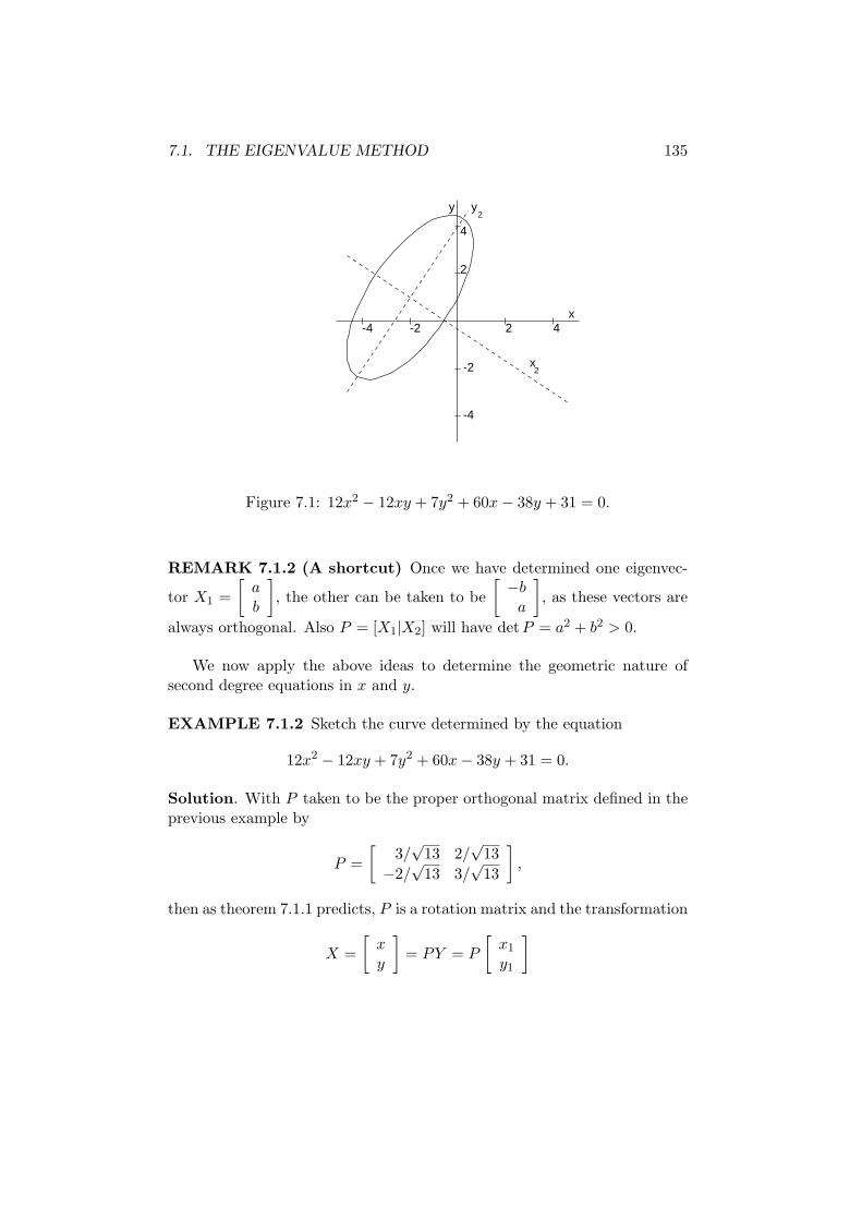
7.1. THE EIGENVALUE METHOD 135
y2
x2
2 4-2-4
2
4
-2
-4
x
y
Figure 7.1: 12x2 − 12xy + 7y2 + 60x − 38y + 31 = 0.
REMARK 7.1.2 (A shortcut) Once we have determined one eigenvec-
tor X1 =
[
ab
]
, the other can be taken to be
[
−ba
]
, as these vectors are
always orthogonal. Also P = [X1|X2] will have detP = a2 + b2 > 0.
We now apply the above ideas to determine the geometric nature ofsecond degree equations in x and y.
EXAMPLE 7.1.2 Sketch the curve determined by the equation
12x2 − 12xy + 7y2 + 60x − 38y + 31 = 0.
Solution. With P taken to be the proper orthogonal matrix defined in theprevious example by
P =
[
3/√
13 2/√
13
−2/√
13 3/√
13
]
,
then as theorem 7.1.1 predicts, P is a rotation matrix and the transformation
X =
[
xy
]
= PY = P
[
x1
y1
]
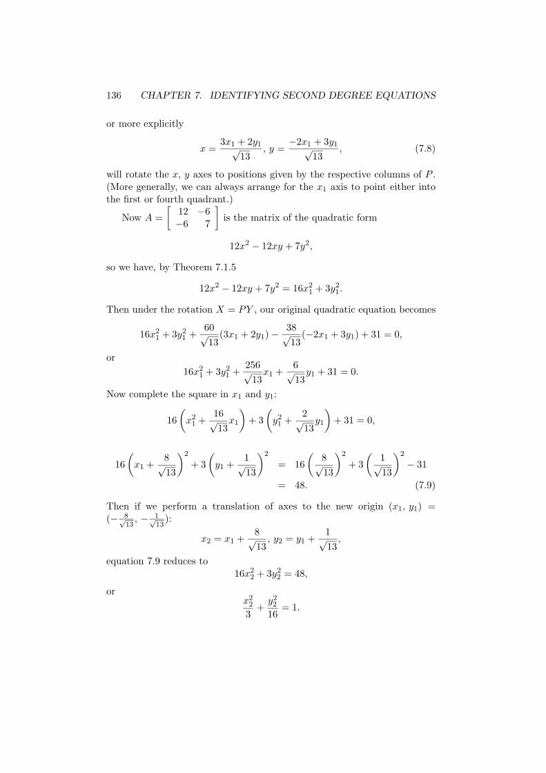
136 CHAPTER 7. IDENTIFYING SECOND DEGREE EQUATIONS
or more explicitly
x =3x1 + 2y1√
13, y =
−2x1 + 3y1√13
, (7.8)
will rotate the x, y axes to positions given by the respective columns of P .(More generally, we can always arrange for the x1 axis to point either intothe first or fourth quadrant.)
Now A =
[
12 −6−6 7
]
is the matrix of the quadratic form
12x2 − 12xy + 7y2,
so we have, by Theorem 7.1.5
12x2 − 12xy + 7y2 = 16x21 + 3y2
1.
Then under the rotation X = PY , our original quadratic equation becomes
16x21 + 3y2
1 +60√13
(3x1 + 2y1) −38√13
(−2x1 + 3y1) + 31 = 0,
or
16x21 + 3y2
1 +256√
13x1 +
6√13
y1 + 31 = 0.
Now complete the square in x1 and y1:
16
(
x21 +
16√13
x1
)
+ 3
(
y21 +
2√13
y1
)
+ 31 = 0,
16
(
x1 +8√13
)2
+ 3
(
y1 +1√13
)2
= 16
(
8√13
)2
+ 3
(
1√13
)2
− 31
= 48. (7.9)
Then if we perform a translation of axes to the new origin (x1, y1) =(− 8√
13, − 1√
13):
x2 = x1 +8√13
, y2 = y1 +1√13
,
equation 7.9 reduces to16x2
2 + 3y22 = 48,
orx2
2
3+
y22
16= 1.
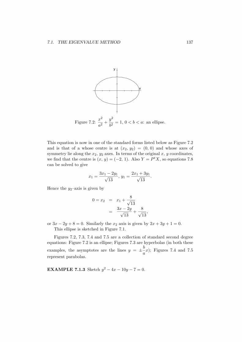
7.1. THE EIGENVALUE METHOD 137
x
y
Figure 7.2:x2
a2+
y2
b2= 1, 0 < b < a: an ellipse.
This equation is now in one of the standard forms listed below as Figure 7.2and is that of a whose centre is at (x2, y2) = (0, 0) and whose axes ofsymmetry lie along the x2, y2 axes. In terms of the original x, y coordinates,we find that the centre is (x, y) = (−2, 1). Also Y = P tX, so equations 7.8can be solved to give
x1 =3x1 − 2y1√
13, y1 =
2x1 + 3y1√13
.
Hence the y2–axis is given by
0 = x2 = x1 +8√13
=3x − 2y√
13+
8√13
,
or 3x − 2y + 8 = 0. Similarly the x2 axis is given by 2x + 3y + 1 = 0.This ellipse is sketched in Figure 7.1.
Figures 7.2, 7.3, 7.4 and 7.5 are a collection of standard second degreeequations: Figure 7.2 is an ellipse; Figures 7.3 are hyperbolas (in both these
examples, the asymptotes are the lines y = ± b
ax); Figures 7.4 and 7.5
represent parabolas.
EXAMPLE 7.1.3 Sketch y2 − 4x − 10y − 7 = 0.
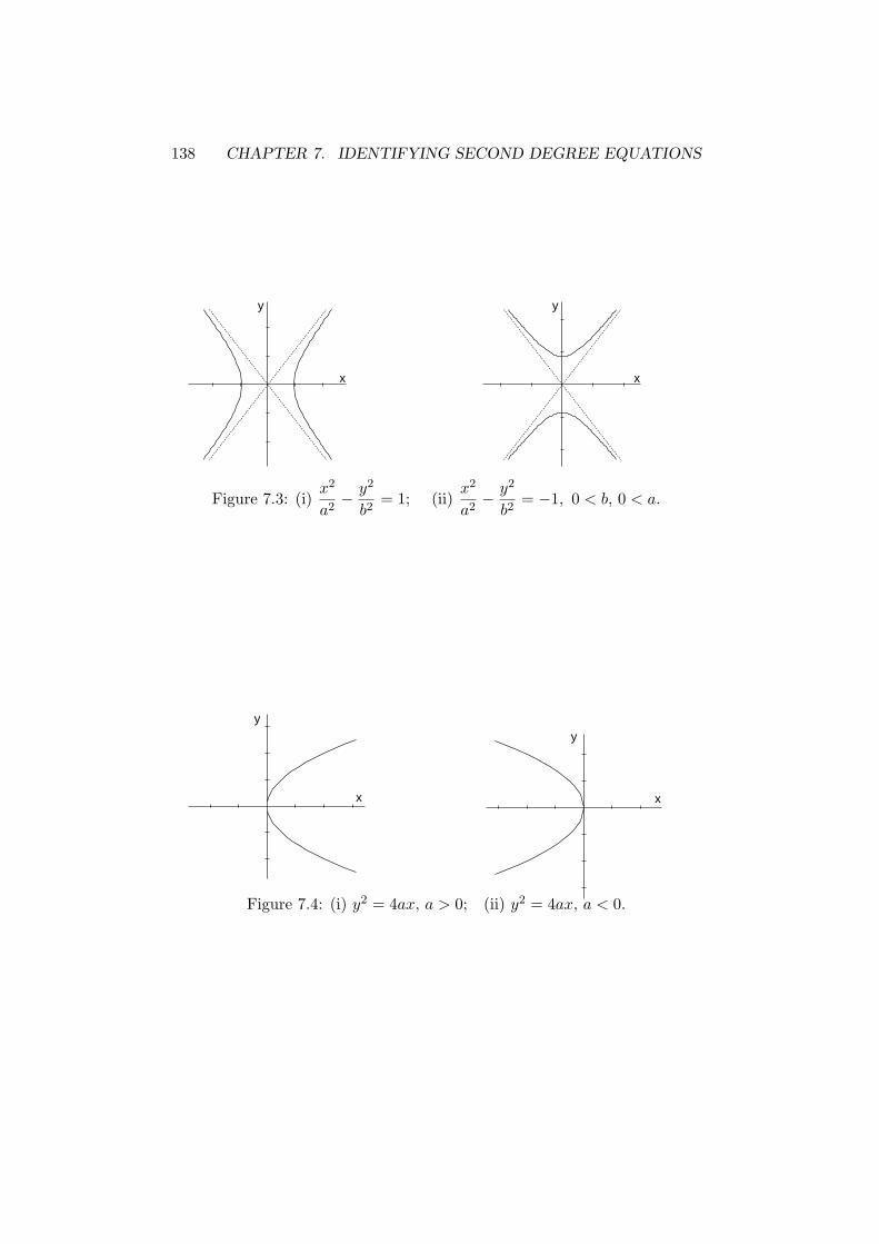
138 CHAPTER 7. IDENTIFYING SECOND DEGREE EQUATIONS
x
y
x
y
Figure 7.3: (i)x2
a2− y2
b2= 1; (ii)
x2
a2− y2
b2= −1, 0 < b, 0 < a.
x
y
x
y
Figure 7.4: (i) y2 = 4ax, a > 0; (ii) y2 = 4ax, a < 0.
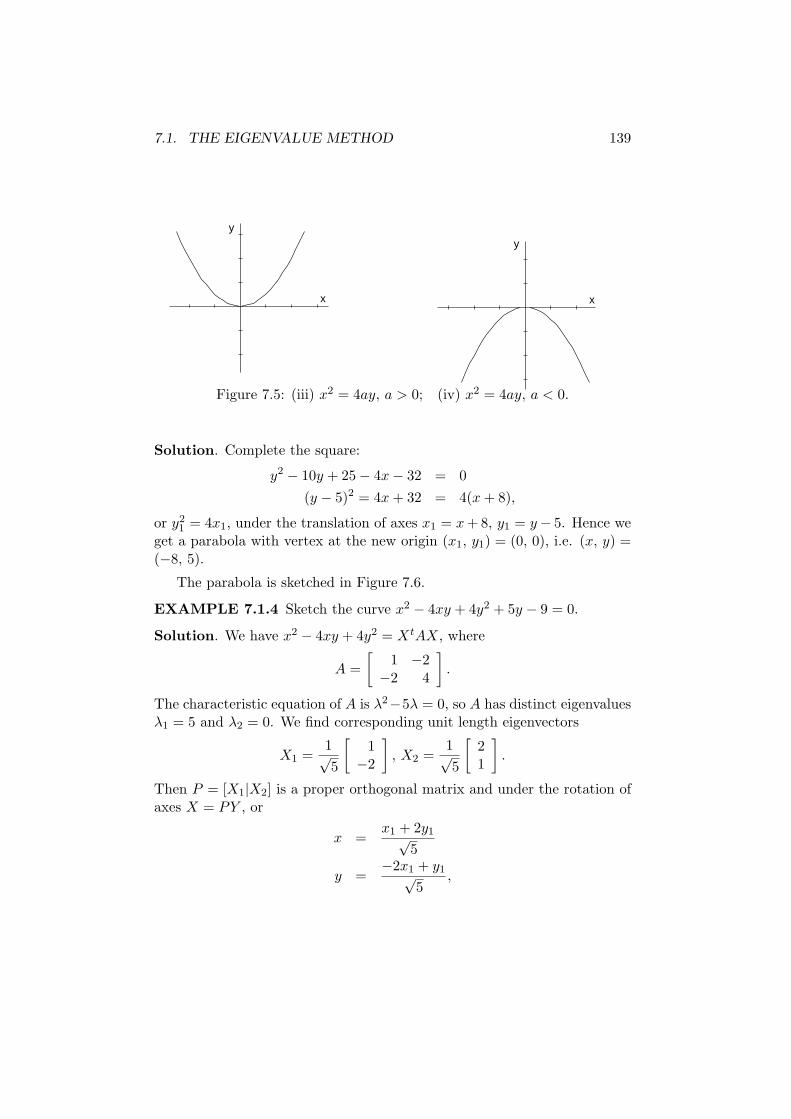
7.1. THE EIGENVALUE METHOD 139
x
y
x
y
Figure 7.5: (iii) x2 = 4ay, a > 0; (iv) x2 = 4ay, a < 0.
Solution. Complete the square:
y2 − 10y + 25 − 4x − 32 = 0
(y − 5)2 = 4x + 32 = 4(x + 8),
or y21 = 4x1, under the translation of axes x1 = x + 8, y1 = y − 5. Hence we
get a parabola with vertex at the new origin (x1, y1) = (0, 0), i.e. (x, y) =(−8, 5).
The parabola is sketched in Figure 7.6.
EXAMPLE 7.1.4 Sketch the curve x2 − 4xy + 4y2 + 5y − 9 = 0.
Solution. We have x2 − 4xy + 4y2 = XtAX, where
A =
[
1 −2−2 4
]
.
The characteristic equation of A is λ2−5λ = 0, so A has distinct eigenvaluesλ1 = 5 and λ2 = 0. We find corresponding unit length eigenvectors
X1 =1√5
[
1−2
]
, X2 =1√5
[
21
]
.
Then P = [X1|X2] is a proper orthogonal matrix and under the rotation ofaxes X = PY , or
x =x1 + 2y1√
5
y =−2x1 + y1√
5,
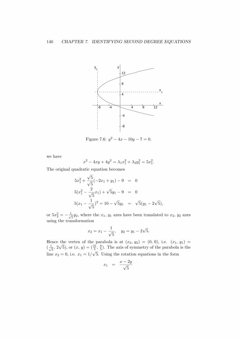
140 CHAPTER 7. IDENTIFYING SECOND DEGREE EQUATIONS
x1
y1
4 8 12-4-8
4
8
12
-4
-8
x
y
Figure 7.6: y2 − 4x − 10y − 7 = 0.
we havex2 − 4xy + 4y2 = λ1x
21 + λ2y
21 = 5x2
1.
The original quadratic equation becomes
5x21 +
√5√5(−2x1 + y1) − 9 = 0
5(x21 −
2√5x1) +
√5y1 − 9 = 0
5(x1 −1√5)2 = 10 −
√5y1 =
√5(y1 − 2
√5),
or 5x22 = − 1√
5y2, where the x1, y1 axes have been translated to x2, y2 axes
using the transformation
x2 = x1 −1√5, y2 = y1 − 2
√5.
Hence the vertex of the parabola is at (x2, y2) = (0, 0), i.e. (x1, y1) =( 1√
5, 2
√5), or (x, y) = (21
5 , 85). The axis of symmetry of the parabola is the
line x2 = 0, i.e. x1 = 1/√
5. Using the rotation equations in the form
x1 =x − 2y√
5
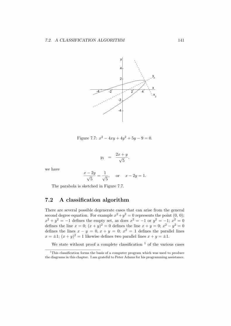
7.2. A CLASSIFICATION ALGORITHM 141
x2
y2
2 4-2-4
2
4
-2
-4
x
y
Figure 7.7: x2 − 4xy + 4y2 + 5y − 9 = 0.
y1 =2x + y√
5,
we havex − 2y√
5=
1√5, or x − 2y = 1.
The parabola is sketched in Figure 7.7.
7.2 A classification algorithm
There are several possible degenerate cases that can arise from the generalsecond degree equation. For example x2 +y2 = 0 represents the point (0, 0);x2 + y2 = −1 defines the empty set, as does x2 = −1 or y2 = −1; x2 = 0defines the line x = 0; (x + y)2 = 0 defines the line x + y = 0; x2 − y2 = 0defines the lines x − y = 0, x + y = 0; x2 = 1 defines the parallel linesx = ±1; (x + y)2 = 1 likewise defines two parallel lines x + y = ±1.
We state without proof a complete classification 1 of the various cases
1This classification forms the basis of a computer program which was used to produce
the diagrams in this chapter. I am grateful to Peter Adams for his programming assistance.
142 CHAPTER 7. IDENTIFYING SECOND DEGREE EQUATIONS
that can possibly arise for the general second degree equation
ax2 + 2hxy + by2 + 2gx + 2fy + c = 0. (7.10)
It turns out to be more convenient to first perform a suitable translation ofaxes, before rotating the axes. Let
∆ =
∣
∣
∣
∣
∣
∣
a h gh b fg f c
∣
∣
∣
∣
∣
∣
, C = ab − h2, A = bc − f2, B = ca − g2.
If C 6= 0, let
α =
−∣
∣
∣
∣
g hf b
∣
∣
∣
∣
C, β =
−∣
∣
∣
∣
a gh f
∣
∣
∣
∣
C. (7.11)
CASE 1. ∆ = 0.
(1.1) C 6= 0. Translate axes to the new origin (α, β), where α and β aregiven by equations 7.11:
x = x1 + α, y = y1 + β.
Then equation 7.10 reduces to
ax21 + 2hx1y1 + by2
1 = 0.
(a) C > 0: Single point (x, y) = (α, β).
(b) C < 0: Two non–parallel lines intersecting in (x, y) = (α, β).
The lines are
y − β
x − α=
−h ±√−C
bif b 6= 0,
x = α andy − β
x − α= − a
2h, if b = 0.
(1.2) C = 0.
(a) h = 0.
(i) a = g = 0.
(A) A > 0: Empty set.
(B) A = 0: Single line y = −f/b.
7.2. A CLASSIFICATION ALGORITHM 143
(C) A < 0: Two parallel lines
y =−f ±
√−A
b
(ii) b = f = 0.
(A) B > 0: Empty set.
(B) B = 0: Single line x = −g/a.
(C) B < 0: Two parallel lines
x =−g ±
√−B
a
(b) h 6= 0.
(i) B > 0: Empty set.
(ii) B = 0: Single line ax + hy = −g.
(iii) B < 0: Two parallel lines
ax + hy = −g ±√−B.
CASE 2. ∆ 6= 0.
(2.1) C 6= 0. Translate axes to the new origin (α, β), where α and β aregiven by equations 7.11:
x = x1 + α, y = y1 + β.
Equation 7.10 becomes
ax21 + 2hx1y1 + by2
1 = −∆
C. (7.12)
CASE 2.1(i) h = 0. Equation 7.12 becomes ax21 + by2
1 = −∆C .
(a) C < 0: Hyperbola.
(b) C > 0 and a∆ > 0: Empty set.
(c) C > 0 and a∆ < 0.
(i) a = b: Circle, centre (α, β), radius√
g2+f2−aca .
(ii) a 6= b: Ellipse.
144 CHAPTER 7. IDENTIFYING SECOND DEGREE EQUATIONS
CASE 2.1(ii) h 6= 0.
Rotate the (x1, y1) axes with the new positive x2–axis in the directionof
[(b − a + R)/2, −h],
where R =√
(a − b)2 + 4h2.
Then equation 7.12 becomes
λ1x22 + λ2y
22 = −∆
C. (7.13)
whereλ1 = (a + b − R)/2, λ2 = (a + b + R)/2,
Here λ1λ2 = C.
(a) C < 0: Hyperbola.
Here λ2 > 0 > λ1 and equation 7.13 becomes
x22
u2− y2
2
v2=
−∆
|∆| ,
where
u =
√
|∆|Cλ1
, v =
√
|∆|−Cλ2
.
(b) C > 0 and a∆ > 0: Empty set.
(c) C > 0 and a∆ < 0: Ellipse.
Here λ1, λ2, a, b have the same sign and λ1 6= λ2 and equa-tion 7.13 becomes
x22
u2+
y22
v2= 1,
where
u =
√
∆
−Cλ1, v =
√
∆
−Cλ2.
(2.1) C = 0.
(a) h = 0.
(i) a = 0: Then b 6= 0 and g 6= 0. Parabola with vertex
(−A
2gb, −f
b
)
.
7.2. A CLASSIFICATION ALGORITHM 145
Translate axes to (x1, y1) axes:
y21 = −2g
bx1.
(ii) b = 0: Then a 6= 0 and f 6= 0. Parabola with vertex
(
−g
a,−B
2fa
)
.
Translate axes to (x1, y1) axes:
x21 = −2f
ay1.
(b) h 6= 0: Parabola. Let
k =ga + hf
a + b.
The vertex of the parabola is
(
(2akf − hk2 − hac)
d,
a(k2 + ac − 2kg)
d
)
,
where d = 2a(gh − af). Now translate to the vertex as the neworigin, then rotate to (x2, y2) axes with the positive x2–axis along[sa, −sh], where s = sign (a).
(The positive x2–axis points into the first or fourth quadrant.)Then the parabola has equation
x22 =
−2st√a2 + h2
y2,
where t = (af − gh)/(a + b).
REMARK 7.2.1 If ∆ = 0, it is not necessary to rotate the axes. Insteadit is always possible to translate the axes suitably so that the coefficients ofthe terms of the first degree vanish.
EXAMPLE 7.2.1 Identify the curve
2x2 + xy − y2 + 6y − 8 = 0. (7.14)
146 CHAPTER 7. IDENTIFYING SECOND DEGREE EQUATIONS
Solution. Here
∆ =
∣
∣
∣
∣
∣
∣
2 12 0
12 −1 30 3 −8
∣
∣
∣
∣
∣
∣
= 0.
Let x = x1 + α, y = y1 + β and substitute in equation 7.14 to get
2(x1 + α)2 + (x1 + α)(y1 + β) − (y1 + β)2 + 4(y1 + β) − 8 = 0. (7.15)
Then equating the coefficients of x1 and y1 to 0 gives
4α + β = 0
α + 2β + 4 = 0,
which has the unique solution α = −23 , β = 8
3 . Then equation 7.15 simplifiesto
2x21 + x1y1 − y2
1 = 0 = (2x1 − y1)(x1 + y1),
so relative to the x1, y1 coordinates, equation 7.14 describes two lines: 2x1−y1 = 0 or x1 + y1 = 0. In terms of the original x, y coordinates, these linesbecome 2(x + 2
3)− (y− 83) = 0 and (x + 2
3) + (y− 83) = 0, i.e. 2x− y + 4 = 0
and x + y − 2 = 0, which intersect in the point
(x, y) = (α, β) = (−2
3,
8
3).
EXAMPLE 7.2.2 Identify the curve
x2 + 2xy + y2 + +2x + 2y + 1 = 0. (7.16)
Solution. Here
∆ =
∣
∣
∣
∣
∣
∣
1 1 11 1 11 1 1
∣
∣
∣
∣
∣
∣
= 0.
Let x = x1 + α, y = y1 + β and substitute in equation 7.16 to get
(x1+α)2+2(x1+α)(y1+β)+(y1+β)2+2(x1+α)+2(y1+β)+1 = 0. (7.17)
Then equating the coefficients of x1 and y1 to 0 gives the same equation
2α + 2β + 2 = 0.
Take α = 0, β = −1. Then equation 7.17 simplifies to
x21 + 2x1y1 + y2
1 = 0 = (x1 + y1)2,
and in terms of x, y coordinates, equation 7.16 becomes
(x + y + 1)2 = 0, or x + y + 1 = 0.
7.3. PROBLEMS 147
7.3 PROBLEMS
1. Sketch the curves
(i) x2 − 8x + 8y + 8 = 0;
(ii) y2 − 12x + 2y + 25 = 0.
2. Sketch the hyperbola4xy − 3y2 = 8
and find the equations of the asymptotes.
[Answer: y = 0 and y = 43x.]
3. Sketch the ellipse8x2 − 4xy + 5y2 = 36
and find the equations of the axes of symmetry.
[Answer: y = 2x and x = −2y.]
4. Sketch the conics defined by the following equations. Find the centrewhen the conic is an ellipse or hyperbola, asymptotes if an hyperbola,the vertex and axis of symmetry if a parabola:
(i) 4x2 − 9y2 − 24x − 36y − 36 = 0;
(ii) 5x2 − 4xy + 8y2 + 4√
5x − 16√
5y + 4 = 0;
(iii) 4x2 + y2 − 4xy − 10y − 19 = 0;
(iv) 77x2 + 78xy − 27y2 + 70x − 30y + 29 = 0.
[Answers: (i) hyperbola, centre (3, −2), asymptotes 2x − 3y − 12 =0, 2x + 3y = 0;
(ii) ellipse, centre (0,√
5);
(iii) parabola, vertex (−75 , −9
5), axis of symmetry 2x − y + 1 = 0;
(iv) hyperbola, centre (− 110 , 7
10), asymptotes 7x + 9y + 7 = 0 and11x − 3y − 1 = 0.]
5. Identify the lines determined by the equations:
(i) 2x2 + y2 + 3xy − 5x − 4y + 3 = 0;
148 CHAPTER 7. IDENTIFYING SECOND DEGREE EQUATIONS
(ii) 9x2 + y2 − 6xy + 6x − 2y + 1 = 0;
(iii) x2 + 4xy + 4y2 − x − 2y − 2 = 0.
[Answers: (i) 2x + y − 3 = 0 and x + y − 1 = 0; (ii) 3x − y + 1 = 0;(iii) x + 2y + 1 = 0 and x + 2y − 2 = 0.]
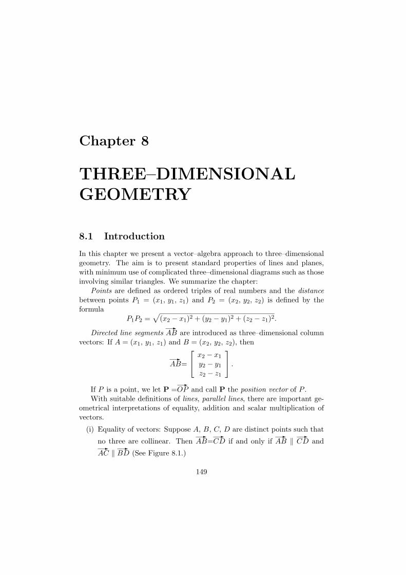
Chapter 8
THREE–DIMENSIONAL
GEOMETRY
8.1 Introduction
In this chapter we present a vector–algebra approach to three–dimensionalgeometry. The aim is to present standard properties of lines and planes,with minimum use of complicated three–dimensional diagrams such as thoseinvolving similar triangles. We summarize the chapter:
Points are defined as ordered triples of real numbers and the distance
between points P1 = (x1, y1, z1) and P2 = (x2, y2, z2) is defined by theformula
P1P2 =√
(x2 − x1)2 + (y2 − y1)2 + (z2 − z1)2.
Directed line segments-
AB are introduced as three–dimensional columnvectors: If A = (x1, y1, z1) and B = (x2, y2, z2), then
-AB=
x2 − x1
y2 − y1
z2 − z1
.
If P is a point, we let P =-
OP and call P the position vector of P .With suitable definitions of lines, parallel lines, there are important ge-
ometrical interpretations of equality, addition and scalar multiplication ofvectors.
(i) Equality of vectors: Suppose A, B, C, D are distinct points such that
no three are collinear. Then-
AB=-
CD if and only if-
AB ‖-
CD and-
AC ‖-
BD (See Figure 8.1.)
149
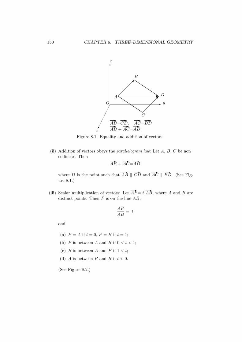
150 CHAPTER 8. THREE–DIMENSIONAL GEOMETRY
¢¢
¢¢
¢¢®
-
6
y
z
x
O
¡¡
¡¡µ
-A
¡¡
¡¡µ
C
D
B
-AB=
-CD,
-AC=
-BD-
AB +-
AC=-
AD
Figure 8.1: Equality and addition of vectors.
(ii) Addition of vectors obeys the parallelogram law: Let A, B, C be non–collinear. Then
-AB +
-AC=
-AD,
where D is the point such that-
AB ‖-
CD and-
AC ‖-
BD. (See Fig-ure 8.1.)
(iii) Scalar multiplication of vectors: Let-
AP= t-
AB, where A and B aredistinct points. Then P is on the line AB,
AP
AB= |t|
and
(a) P = A if t = 0, P = B if t = 1;
(b) P is between A and B if 0 < t < 1;
(c) B is between A and P if 1 < t;
(d) A is between P and B if t < 0.
(See Figure 8.2.)
8.1. INTRODUCTION 151
¢¢
¢¢
¢¢®
-
6
y
z
x
O
@@
@@
@R
@@
@R P
A
B
-AP= t
-AB, 0 < t < 1
Figure 8.2: Scalar multiplication of vectors.
The dot product X ·Y of vectors X =
a1
b1
c1
and Y =
a2
b2
c2
, is defined
by
X · Y = a1a2 + b1b2 + c1c2.
The length ||X|| of a vector X is defined by
||X|| = (X · X)1/2
and the Cauchy–Schwarz inequality holds:
|X · Y | ≤ ||X|| · ||Y ||.
The triangle inequality for vector length now follows as a simple deduction:
||X + Y || ≤ ||X|| + ||Y ||.
Using the equation
AB = ||-
AB ||,
we deduce the corresponding familiar triangle inequality for distance:
AB ≤ AC + CB.
152 CHAPTER 8. THREE–DIMENSIONAL GEOMETRY
The angle θ between two non–zero vectors X and Y is then defined by
cos θ =X · Y
||X|| · ||Y || , 0 ≤ θ ≤ π.
This definition makes sense. For by the Cauchy–Schwarz inequality,
−1 ≤ X · Y||X|| · ||Y || ≤ 1.
Vectors X and Y are said to be perpendicular or orthogonal if X ·Y = 0.Vectors of unit length are called unit vectors. The vectors
i =
100
, j =
010
, k =
001
are unit vectors and every vector is a linear combination of i, j and k:
abc
= ai + bj + ck.
Non–zero vectors X and Y are parallel or proportional if the angle be-tween X and Y equals 0 or π; equivalently if X = tY for some real numbert. Vectors X and Y are then said to have the same or opposite direction,according as t > 0 or t < 0.
We are then led to study straight lines. If A and B are distinct points,it is easy to show that AP + PB = AB holds if and only if
-AP= t
-AB, where 0 ≤ t ≤ 1.
A line is defined as a set consisting of all points P satisfying
P = P0 + tX, t ∈ R or equivalently-
P0P= tX,
for some fixed point P0 and fixed non–zero vector X called a direction vector
for the line.Equivalently, in terms of coordinates,
x = x0 + ta, y = y0 + tb, z = z0 + tc,
where P0 = (x0, y0, z0) and not all of a, b, c are zero.
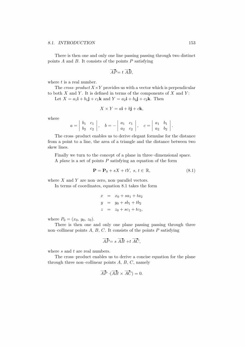
8.1. INTRODUCTION 153
There is then one and only one line passing passing through two distinctpoints A and B. It consists of the points P satisfying
-AP= t
-AB,
where t is a real number.The cross–product X×Y provides us with a vector which is perpendicular
to both X and Y . It is defined in terms of the components of X and Y :Let X = a1i + b1j + c1k and Y = a2i + b2j + c2k. Then
X × Y = ai + bj + ck,
where
a =
∣
∣
∣
∣
b1 c1
b2 c2
∣
∣
∣
∣
, b = −∣
∣
∣
∣
a1 c1
a2 c2
∣
∣
∣
∣
, c =
∣
∣
∣
∣
a1 b1
a2 b2
∣
∣
∣
∣
.
The cross–product enables us to derive elegant formulae for the distancefrom a point to a line, the area of a triangle and the distance between twoskew lines.
Finally we turn to the concept of a plane in three–dimensional space.A plane is a set of points P satisfying an equation of the form
P = P0 + sX + tY, s, t ∈ R, (8.1)
where X and Y are non–zero, non–parallel vectors.In terms of coordinates, equation 8.1 takes the form
x = x0 + sa1 + ta2
y = y0 + sb1 + tb2
z = z0 + sc1 + tc2,
where P0 = (x0, y0, z0).There is then one and only one plane passing passing through three
non–collinear points A, B, C. It consists of the points P satisfying
-AP= s
-AB +t
-AC,
where s and t are real numbers.The cross–product enables us to derive a concise equation for the plane
through three non–collinear points A, B, C, namely
-AP ·(
-AB ×
-AC) = 0.
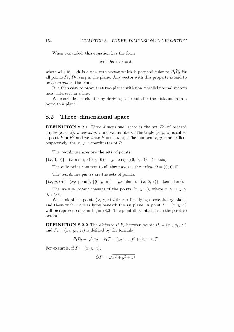
154 CHAPTER 8. THREE–DIMENSIONAL GEOMETRY
When expanded, this equation has the form
ax + by + cz = d,
where ai + bj + ck is a non–zero vector which is perpendicular to-
P1P2 forall points P1, P2 lying in the plane. Any vector with this property is said tobe a normal to the plane.
It is then easy to prove that two planes with non–parallel normal vectorsmust intersect in a line.
We conclude the chapter by deriving a formula for the distance from apoint to a plane.
8.2 Three–dimensional space
DEFINITION 8.2.1 Three–dimensional space is the set E3 of orderedtriples (x, y, z), where x, y, z are real numbers. The triple (x, y, z) is calleda point P in E3 and we write P = (x, y, z). The numbers x, y, z are called,respectively, the x, y, z coordinates of P .
The coordinate axes are the sets of points:
{(x, 0, 0)} (x–axis), {(0, y, 0)} (y–axis), {(0, 0, z)} (z–axis).
The only point common to all three axes is the origin O = (0, 0, 0).
The coordinate planes are the sets of points:
{(x, y, 0)} (xy–plane), {(0, y, z)} (yz–plane), {(x, 0, z)} (xz–plane).
The positive octant consists of the points (x, y, z), where x > 0, y >0, z > 0.
We think of the points (x, y, z) with z > 0 as lying above the xy–plane,and those with z < 0 as lying beneath the xy–plane. A point P = (x, y, z)will be represented as in Figure 8.3. The point illustrated lies in the positiveoctant.
DEFINITION 8.2.2 The distance P1P2 between points P1 = (x1, y1, z1)and P2 = (x2, y2, z2) is defined by the formula
P1P2 =√
(x2 − x1)2 + (y2 − y1)2 + (z2 − z1)2.
For example, if P = (x, y, z),
OP =√
x2 + y2 + z2.
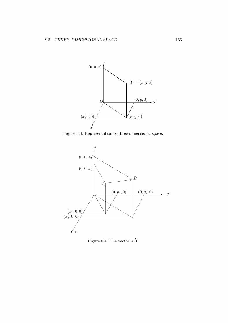
8.2. THREE–DIMENSIONAL SPACE 155
¢¢
¢¢
¢¢®
-
6
y
z
x
OQ
Q (x, y, 0)(x, 0, 0) ¢¢¢¢(0, y, 0)
P = (x, y, z)
(0, 0, z)
P = (x, y, z)
Figure 8.3: Representation of three-dimensional space.
- y·
··
··
··
··
·À x
(x2, 0, 0)(x1, 0, 0)
(0, y1, 0) (0, y2, 0)
(0, 0, z1)
(0, 0, z2)
6z
bb
bb
bb
bb
bb
¢¢¢¢¢¢
bb
bb
bb
bb
bb
TT
TT
T
·····
TT
TT
T
A
B
Figure 8.4: The vector-
AB.
156 CHAPTER 8. THREE–DIMENSIONAL GEOMETRY
DEFINITION 8.2.3 If A = (x1, y1, z1) and B = (x2, y2, z2) we define
the symbol-
AB to be the column vector
-AB=
x2 − x1
y2 − y1
z2 − z1
.
We let P =-
OP and call P the position vector of P .
The components of-
AB are the coordinates of B when the axes aretranslated to A as origin of coordinates.
We think of-
AB as being represented by the directed line segment fromA to B and think of it as an arrow whose tail is at A and whose head is atB. (See Figure 8.4.)
Some mathematicians think of-
AB as representing the translation ofspace which takes A into B.
The following simple properties of-
AB are easily verified and correspondto how we intuitively think of directed line segments:
(i)-
AB= 0 ⇔ A = B;
(ii)-
BA= −-
AB;
(iii)-
AB +-
BC=-
AC (the triangle law);
(iv)-
BC=-
AC −-
AB= C − B;
(v) if X is a vector and A a point, there is exactly one point B such that-
AB= X, namely that defined by B = A + X.
To derive properties of the distance function and the vector function-
P1P2, we need to introduce the dot product of two vectors in R3.
8.3 Dot product
DEFINITION 8.3.1 If X =
a1
b1
c1
and Y =
a2
b2
c2
, then X · Y , the
dot product of X and Y , is defined by
X · Y = a1a2 + b1b2 + c1c2.
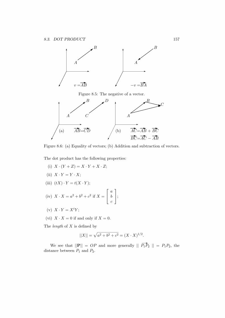
8.3. DOT PRODUCT 157
¢¢
¢¢®
¢¢
¢¢®
¢¢
¢¢®
¢¢
¢¢®
- -
6 6
½½
½½> ½
½½
½=A
B
A
B
v =-
AB −v =-
BA
Figure 8.5: The negative of a vector.
¢¢
¢¢®
¢¢
¢¢®
¢¢
¢¢®
- -
6 6
½½
½½>
½½
½½>
½½
½½>
»»»»»»»»:XXXXz
A
B
C
D
A
BC
(a) (b)-
AB=-
CD-
AC=-
AB +-
BC-
BC=-
AC −-
AB
Figure 8.6: (a) Equality of vectors; (b) Addition and subtraction of vectors.
The dot product has the following properties:
(i) X · (Y + Z) = X · Y + X · Z;
(ii) X · Y = Y · X;
(iii) (tX) · Y = t(X · Y );
(iv) X · X = a2 + b2 + c2 if X =
abc
;
(v) X · Y = XtY ;
(vi) X · X = 0 if and only if X = 0.
The length of X is defined by
||X|| =√
a2 + b2 + c2 = (X · X)1/2.
We see that ||P|| = OP and more generally ||-
P1P2 || = P1P2, thedistance between P1 and P2.
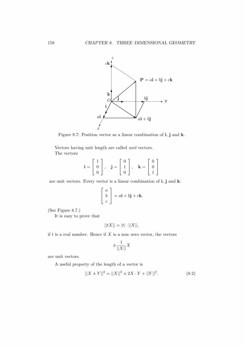
158 CHAPTER 8. THREE–DIMENSIONAL GEOMETRY
¢¢
¢¢
¢¢®
-
6
y
z
x
O
,,
,,
,,
¢¢
¢®®
i
-j
6
-
6ck
k
QQs ai + bjai ¢
¢¢¢bj
P = ai + bj + ck
Figure 8.7: Position vector as a linear combination of i, j and k.
Vectors having unit length are called unit vectors.The vectors
i =
100
, j =
010
, k =
001
are unit vectors. Every vector is a linear combination of i, j and k:
abc
= ai + bj + ck.
(See Figure 8.7.)It is easy to prove that
||tX|| = |t| · ||X||,
if t is a real number. Hence if X is a non–zero vector, the vectors
± 1
||X||X
are unit vectors.
A useful property of the length of a vector is
||X ± Y ||2 = ||X||2 ± 2X · Y + ||Y ||2. (8.2)
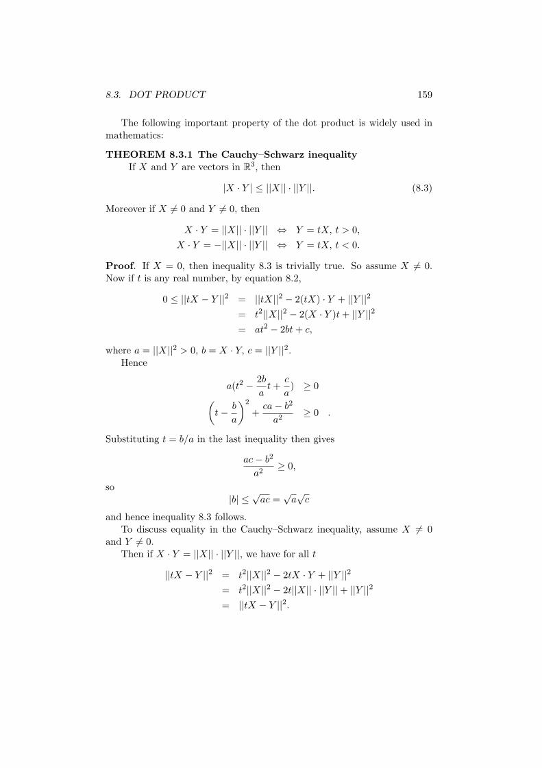
8.3. DOT PRODUCT 159
The following important property of the dot product is widely used inmathematics:
THEOREM 8.3.1 The Cauchy–Schwarz inequalityIf X and Y are vectors in R3, then
|X · Y | ≤ ||X|| · ||Y ||. (8.3)
Moreover if X 6= 0 and Y 6= 0, then
X · Y = ||X|| · ||Y || ⇔ Y = tX, t > 0,
X · Y = −||X|| · ||Y || ⇔ Y = tX, t < 0.
Proof. If X = 0, then inequality 8.3 is trivially true. So assume X 6= 0.Now if t is any real number, by equation 8.2,
0 ≤ ||tX − Y ||2 = ||tX||2 − 2(tX) · Y + ||Y ||2= t2||X||2 − 2(X · Y )t + ||Y ||2= at2 − 2bt + c,
where a = ||X||2 > 0, b = X · Y, c = ||Y ||2.Hence
a(t2 − 2b
at +
c
a) ≥ 0
(
t − b
a
)2
+ca − b2
a2≥ 0 .
Substituting t = b/a in the last inequality then gives
ac − b2
a2≥ 0,
so|b| ≤ √
ac =√
a√
c
and hence inequality 8.3 follows.To discuss equality in the Cauchy–Schwarz inequality, assume X 6= 0
and Y 6= 0.Then if X · Y = ||X|| · ||Y ||, we have for all t
||tX − Y ||2 = t2||X||2 − 2tX · Y + ||Y ||2= t2||X||2 − 2t||X|| · ||Y || + ||Y ||2= ||tX − Y ||2.
160 CHAPTER 8. THREE–DIMENSIONAL GEOMETRY
Taking t = ||X||/||Y || then gives ||tX − Y ||2 = 0 and hence tX − Y = 0.Hence Y = tX, where t > 0. The case X · Y = −||X|| · ||Y || is provedsimilarly.
COROLLARY 8.3.1 (The triangle inequality for vectors)If X and Y are vectors, then
||X + Y || ≤ ||X|| + ||Y ||. (8.4)
Moreover if X 6= 0 and Y 6= 0, then equality occurs in inequality 8.4 if andonly if Y = tX, where t > 0.
Proof.
||X + Y ||2 = ||X||2 + 2X · Y + ||Y ||2≤ ||X||2 + 2||X|| · ||Y || + ||Y ||2= (||X|| + ||Y ||)2
and inequality 8.4 follows.
If ||X + Y || = ||X|| + ||Y ||, then the above proof shows that
X · Y = ||X|| · ||Y ||.
Hence if X 6= 0 and Y 6= 0, the first case of equality in the Cauchy–Schwarzinequality shows that Y = tX with t > 0.
The triangle inequality for vectors gives rise to a corresponding inequalityfor the distance function:
THEOREM 8.3.2 (The triangle inequality for distance)If A, B, C are points, then
AC ≤ AB + BC. (8.5)
Moreover if B 6= A and B 6= C, then equality occurs in inequality 8.5 if and
only if-
AB= r-
AC, where 0 < r < 1.
Proof.
AC = ||-
AC || = ||-
AB +-
BC ||≤ ||
-AB || + ||
-BC ||
= AB + BC.
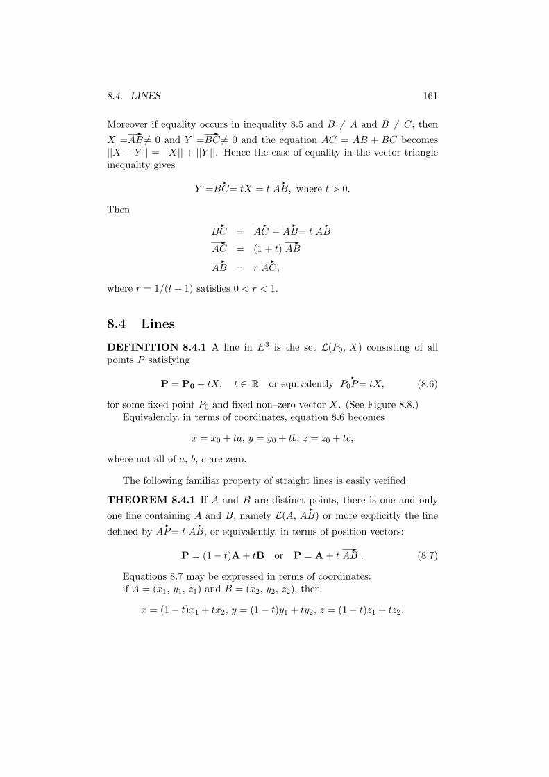
8.4. LINES 161
Moreover if equality occurs in inequality 8.5 and B 6= A and B 6= C, then
X =-
AB 6= 0 and Y =-
BC 6= 0 and the equation AC = AB + BC becomes||X + Y || = ||X|| + ||Y ||. Hence the case of equality in the vector triangleinequality gives
Y =-
BC= tX = t-
AB, where t > 0.
Then
-BC =
-AC −
-AB= t
-AB
-AC = (1 + t)
-AB
-AB = r
-AC,
where r = 1/(t + 1) satisfies 0 < r < 1.
8.4 Lines
DEFINITION 8.4.1 A line in E3 is the set L(P0, X) consisting of allpoints P satisfying
P = P0 + tX, t ∈ R or equivalently-
P0P= tX, (8.6)
for some fixed point P0 and fixed non–zero vector X. (See Figure 8.8.)Equivalently, in terms of coordinates, equation 8.6 becomes
x = x0 + ta, y = y0 + tb, z = z0 + tc,
where not all of a, b, c are zero.
The following familiar property of straight lines is easily verified.
THEOREM 8.4.1 If A and B are distinct points, there is one and only
one line containing A and B, namely L(A,-
AB) or more explicitly the line
defined by-
AP= t-
AB, or equivalently, in terms of position vectors:
P = (1 − t)A + tB or P = A + t-
AB . (8.7)
Equations 8.7 may be expressed in terms of coordinates:if A = (x1, y1, z1) and B = (x2, y2, z2), then
x = (1 − t)x1 + tx2, y = (1 − t)y1 + ty2, z = (1 − t)z1 + tz2.
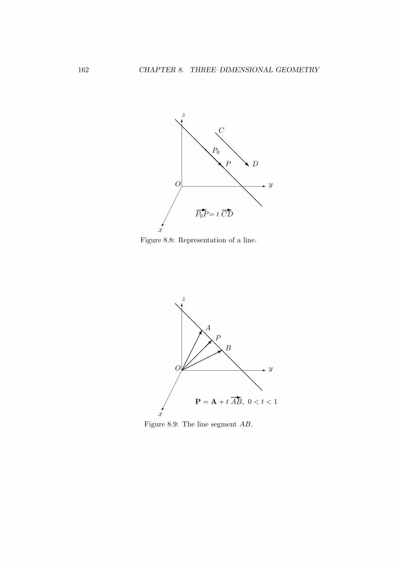
162 CHAPTER 8. THREE–DIMENSIONAL GEOMETRY
¢¢
¢¢
¢¢®
-
6
y
z
x
O
P
P0@@
@R
@@
@@
@R
C
D
@@
@@
@@
@@
@@
@@
@-P0P= t
-CD
Figure 8.8: Representation of a line.
¢¢
¢¢
¢¢®
-
6
y
z
x
O©©©©©©* B
¢¢¢¢¢¢
¡¡
¡¡¡µ
A
P
@@
@@
@@
@@
@@
@@
@
P = A + t-
AB, 0 < t < 1
Figure 8.9: The line segment AB.
8.4. LINES 163
There is an important geometric significance in the number t of the aboveequation of the line through A and B. The proof is left as an exercise:
THEOREM 8.4.2 (Joachimsthal’s ratio formulae)If t is the parameter occurring in theorem 8.4.1, then
(i) |t| =AP
AB; (ii)
∣
∣
∣
∣
t
1 − t
∣
∣
∣
∣
=AP
PBif P 6= B.
Also
(iii) P is between A and B if 0 < t < 1;
(iv) B is between A and P if 1 < t;
(v) A is between P and B if t < 0.
(See Figure 8.9.)For example, t = 1
2 gives the mid–point P of the segment AB:
P =1
2(A + B).
EXAMPLE 8.4.1 L is the line AB, where A = (−4, 3, 1), B = (1, 1, 0);M is the line CD, where C = (2, 0, 2), D = (−1, 3, −2); N is the line EF ,where E = (1, 4, 7), F = (−4, −3, −13). Find which pairs of lines intersectand also the points of intersection.
Solution. In fact only L and N intersect, in the point (−23 , 5
3 , 13). For
example, to determine if L and N meet, we start with vector equations forL and N :
P = A + t-
AB, Q = E + s-
EF,
equate P and Q and solve for s and t:
(−4i + 3j + k) + t(5i − 2j − k) = (i + 4j + 7k) + s(−5i − 7j − 20k),
which on simplifying, gives
5t + 5s = 5
−2t + 7s = 1
−t + 20s = 6
This system has the unique solution t = 23 , s = 1
3 and this determines acorresponding point P where the lines meet, namely P = (−2
3 , 53 , 1
3).The same method yields inconsistent systems when applied to the other
pairs of lines.
164 CHAPTER 8. THREE–DIMENSIONAL GEOMETRY
EXAMPLE 8.4.2 If A = (5, 0, 7) and B = (2, −3, 6), find the points Pon the line AB which satisfy AP/PB = 3.
Solution. Use the formulae
P = A + t-
AB and
∣
∣
∣
∣
t
1 − t
∣
∣
∣
∣
=AP
PB= 3.
Thent
1 − t= 3 or − 3,
so t = 34 or t = 3
2 . The corresponding points are (114 , 9
4 , 254 ) and (1
2 , 92 , 11
2 ).
DEFINITION 8.4.2 Let X and Y be non–zero vectors. Then X is parallel
or proportional to Y if X = tY for some t ∈ R. We write X‖Y if X is parallelto Y . If X = tY , we say that X and Y have the same or opposite direction,according as t > 0 or t < 0.
DEFINITION 8.4.3 if A and B are distinct points on a line L, the non–
zero vector-
AB is called a direction vector for L.
It is easy to prove that any two direction vectors for a line are parallel.
DEFINITION 8.4.4 Let L and M be lines having direction vectors Xand Y , respectively. Then L is parallel to M if X is parallel to Y . Clearlyany line is parallel to itself.
It is easy to prove that the line through a given point A and parallel to a
given line CD has an equation P = A + t-
CD.
THEOREM 8.4.3 Let X = a1i + b1j + c1k and Y = a2i + b2j + c2k benon–zero vectors. Then X is parallel to Y if and only if
∣
∣
∣
∣
a1 b1
a2 b2
∣
∣
∣
∣
=
∣
∣
∣
∣
b1 c1
b2 c2
∣
∣
∣
∣
=
∣
∣
∣
∣
a1 c1
a2 c2
∣
∣
∣
∣
= 0. (8.8)
Proof. The case equality in the Cauchy–Schwarz inequality (Theorem 8.3.1)shows that X and Y are parallel if and only if
|X · Y | = ||X|| · ||Y ||.
Squaring gives the equivalent equality
(a1a2 + b1b2 + c1c2)2 = (a2
1 + b21 + c2
1)(a22 + b2
2 + c22),
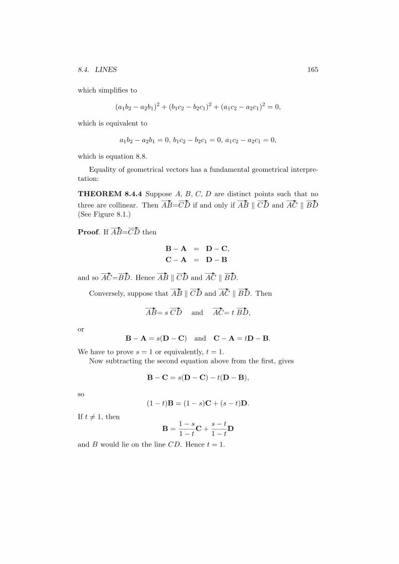
8.4. LINES 165
which simplifies to
(a1b2 − a2b1)2 + (b1c2 − b2c1)
2 + (a1c2 − a2c1)2 = 0,
which is equivalent to
a1b2 − a2b1 = 0, b1c2 − b2c1 = 0, a1c2 − a2c1 = 0,
which is equation 8.8.
Equality of geometrical vectors has a fundamental geometrical interpre-tation:
THEOREM 8.4.4 Suppose A, B, C, D are distinct points such that no
three are collinear. Then-
AB=-
CD if and only if-
AB ‖-
CD and-
AC ‖-
BD(See Figure 8.1.)
Proof. If-
AB=-
CD then
B − A = D − C,
C − A = D − B
and so-
AC=-
BD. Hence-
AB ‖-
CD and-
AC ‖-
BD.
Conversely, suppose that-
AB ‖-
CD and-
AC ‖-
BD. Then
-AB= s
-CD and
-AC= t
-BD,
or
B − A = s(D − C) and C − A = tD − B.
We have to prove s = 1 or equivalently, t = 1.Now subtracting the second equation above from the first, gives
B − C = s(D − C) − t(D − B),
so
(1 − t)B = (1 − s)C + (s − t)D.
If t 6= 1, then
B =1 − s
1 − tC +
s − t
1 − tD
and B would lie on the line CD. Hence t = 1.
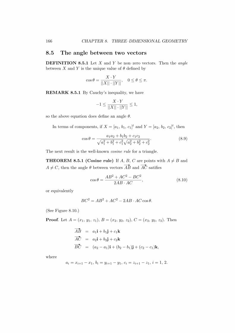
166 CHAPTER 8. THREE–DIMENSIONAL GEOMETRY
8.5 The angle between two vectors
DEFINITION 8.5.1 Let X and Y be non–zero vectors. Then the angle
between X and Y is the unique value of θ defined by
cos θ =X · Y
||X|| · ||Y || , 0 ≤ θ ≤ π.
REMARK 8.5.1 By Cauchy’s inequality, we have
−1 ≤ X · Y||X|| · ||Y || ≤ 1,
so the above equation does define an angle θ.
In terms of components, if X = [a1, b1, c1]t and Y = [a2, b2, c2]
t, then
cos θ =a1a2 + b1b2 + c1c2
√
a21 + b2
1 + c21
√
a22 + b2
2 + c22
. (8.9)
The next result is the well-known cosine rule for a triangle.
THEOREM 8.5.1 (Cosine rule) If A, B, C are points with A 6= B and
A 6= C, then the angle θ between vectors-
AB and-
AC satifies
cos θ =AB2 + AC2 − BC2
2AB · AC, (8.10)
or equivalently
BC2 = AB2 + AC2 − 2AB · AC cos θ.
(See Figure 8.10.)
Proof. Let A = (x1, y1, z1), B = (x2, y2, z2), C = (x3, y3, z3). Then
-AB = a1i + b1j + c1k-
AC = a2i + b2j + c2k-
BC = (a2 − a1)i + (b2 − b1)j + (c2 − c1)k,
where
ai = xi+1 − x1, bi = yi+1 − y1, ci = zi+1 − z1, i = 1, 2.
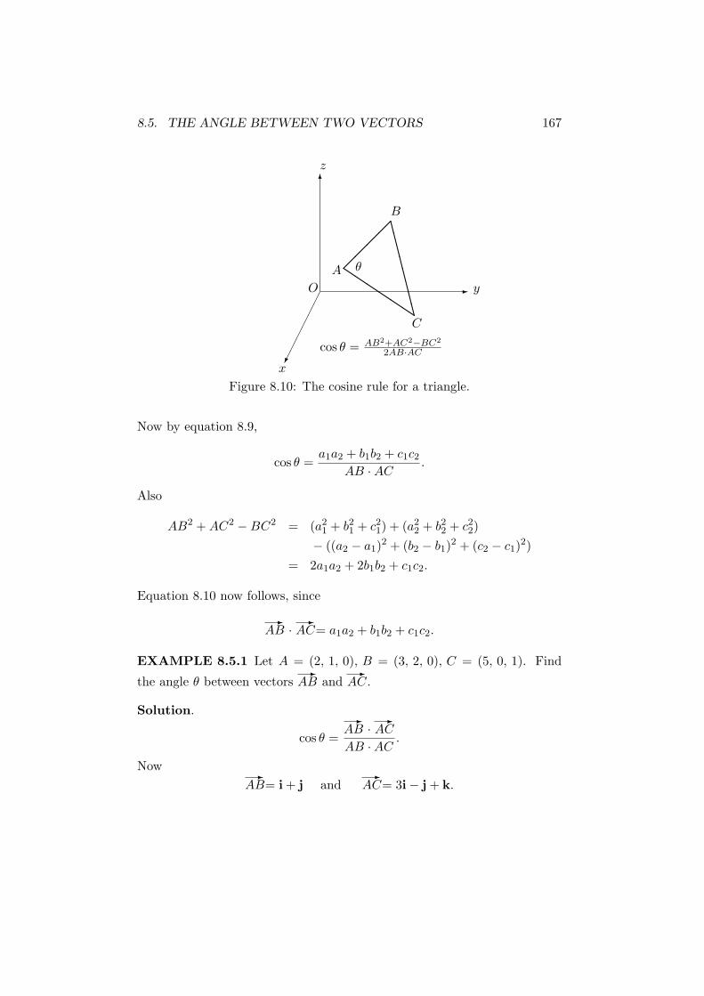
8.5. THE ANGLE BETWEEN TWO VECTORS 167
¢¢
¢¢
¢¢®
-
6
y
z
x
O
¡¡
¡¡
A
CCCCCCCCC
B
θ
cos θ = AB2+AC2−BC2
2AB·AC
Figure 8.10: The cosine rule for a triangle.
Now by equation 8.9,
cos θ =a1a2 + b1b2 + c1c2
AB · AC.
Also
AB2 + AC2 − BC2 = (a21 + b2
1 + c21) + (a2
2 + b22 + c2
2)
− ((a2 − a1)2 + (b2 − b1)
2 + (c2 − c1)2)
= 2a1a2 + 2b1b2 + c1c2.
Equation 8.10 now follows, since
-AB ·
-AC= a1a2 + b1b2 + c1c2.
EXAMPLE 8.5.1 Let A = (2, 1, 0), B = (3, 2, 0), C = (5, 0, 1). Find
the angle θ between vectors-
AB and-
AC.
Solution.
cos θ =
-AB ·
-AC
AB · AC.
Now-
AB= i + j and-
AC= 3i − j + k.
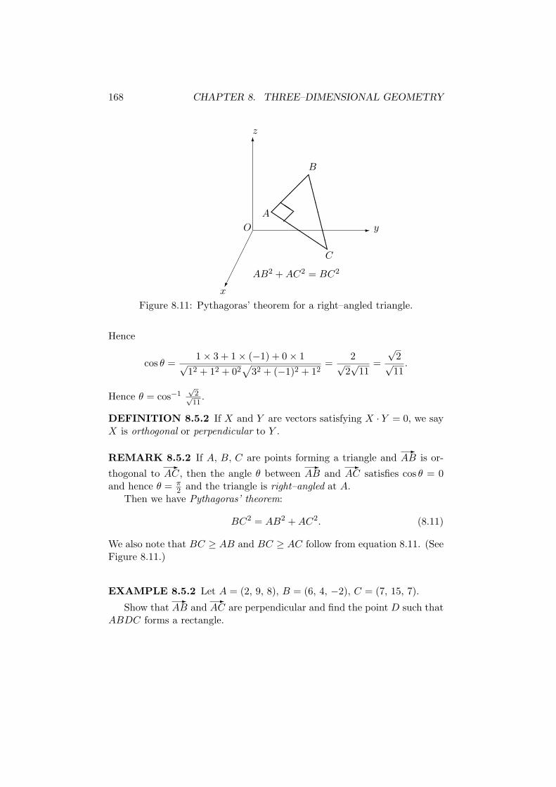
168 CHAPTER 8. THREE–DIMENSIONAL GEOMETRY
¢¢
¢¢
¢¢®
-
6
y
z
x
O¡
QQA
CCCCCCCCC
QQ¡
¡¡
¡B
AB2 + AC2 = BC2
Figure 8.11: Pythagoras’ theorem for a right–angled triangle.
Hence
cos θ =1 × 3 + 1 × (−1) + 0 × 1√
12 + 12 + 02√
32 + (−1)2 + 12=
2√2√
11=
√2√11
.
Hence θ = cos−1√
2√11
.
DEFINITION 8.5.2 If X and Y are vectors satisfying X · Y = 0, we sayX is orthogonal or perpendicular to Y .
REMARK 8.5.2 If A, B, C are points forming a triangle and-
AB is or-
thogonal to-
AC, then the angle θ between-
AB and-
AC satisfies cos θ = 0and hence θ = π
2 and the triangle is right–angled at A.Then we have Pythagoras’ theorem:
BC2 = AB2 + AC2. (8.11)
We also note that BC ≥ AB and BC ≥ AC follow from equation 8.11. (SeeFigure 8.11.)
EXAMPLE 8.5.2 Let A = (2, 9, 8), B = (6, 4, −2), C = (7, 15, 7).
Show that-
AB and-
AC are perpendicular and find the point D such thatABDC forms a rectangle.

8.5. THE ANGLE BETWEEN TWO VECTORS 169
¢¢
¢¢
¢¢®
-
6
y
z
x
OCCCCCCCC
¡@
ÃÃÃÃÃ
@@
@@
@@
@@
@@
@
C
A
B
P
¡¡
¡
Figure 8.12: Distance from a point to a line.
Solution.
-AB ·
-AC= (4i − 5j − 10k) · (5i + 6j − k) = 20 − 30 + 10 = 0.
Hence-
AB and-
AC are perpendicular. Also, the required fourth point Dclearly has to satisfy the equation
-BD=
-AC, or equivalently D − B =
-AC .
Hence
D = B+-
AC= (6i + 4j − 2k) + (5i + 6j − k) = 11i + 10j − 3k,
so D = (11, 10, −3).
THEOREM 8.5.2 (Distance from a point to a line) If C is a pointand L is the line through A and B, then there is exactly one point P on Lsuch that
-CP is perpendicular to
-AB, namely
P = A + t-
AB, t =
-AC ·
-AB
AB2. (8.12)
Moreover if Q is any point on L, then CQ ≥ CP and hence P is the pointon L closest to C.
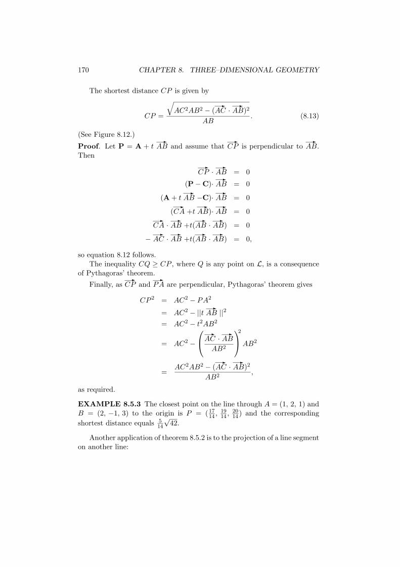
170 CHAPTER 8. THREE–DIMENSIONAL GEOMETRY
The shortest distance CP is given by
CP =
√
AC2AB2 − (-
AC ·-
AB)2
AB. (8.13)
(See Figure 8.12.)
Proof. Let P = A + t-
AB and assume that-
CP is perpendicular to-
AB.Then
-CP ·
-AB = 0
(P − C)·-
AB = 0
(A + t-
AB −C)·-
AB = 0
(-
CA +t-
AB)·-
AB = 0-
CA ·-
AB +t(-
AB ·-
AB) = 0
−-
AC ·-
AB +t(-
AB ·-
AB) = 0,
so equation 8.12 follows.The inequality CQ ≥ CP , where Q is any point on L, is a consequence
of Pythagoras’ theorem.
Finally, as-
CP and-
PA are perpendicular, Pythagoras’ theorem gives
CP 2 = AC2 − PA2
= AC2 − ||t-
AB ||2= AC2 − t2AB2
= AC2 −
-AC ·
-AB
AB2
2
AB2
=AC2AB2 − (
-AC ·
-AB)2
AB2,
as required.
EXAMPLE 8.5.3 The closest point on the line through A = (1, 2, 1) andB = (2, −1, 3) to the origin is P = (17
14 , 1914 , 20
14) and the corresponding
shortest distance equals 514
√42.
Another application of theorem 8.5.2 is to the projection of a line segmenton another line:
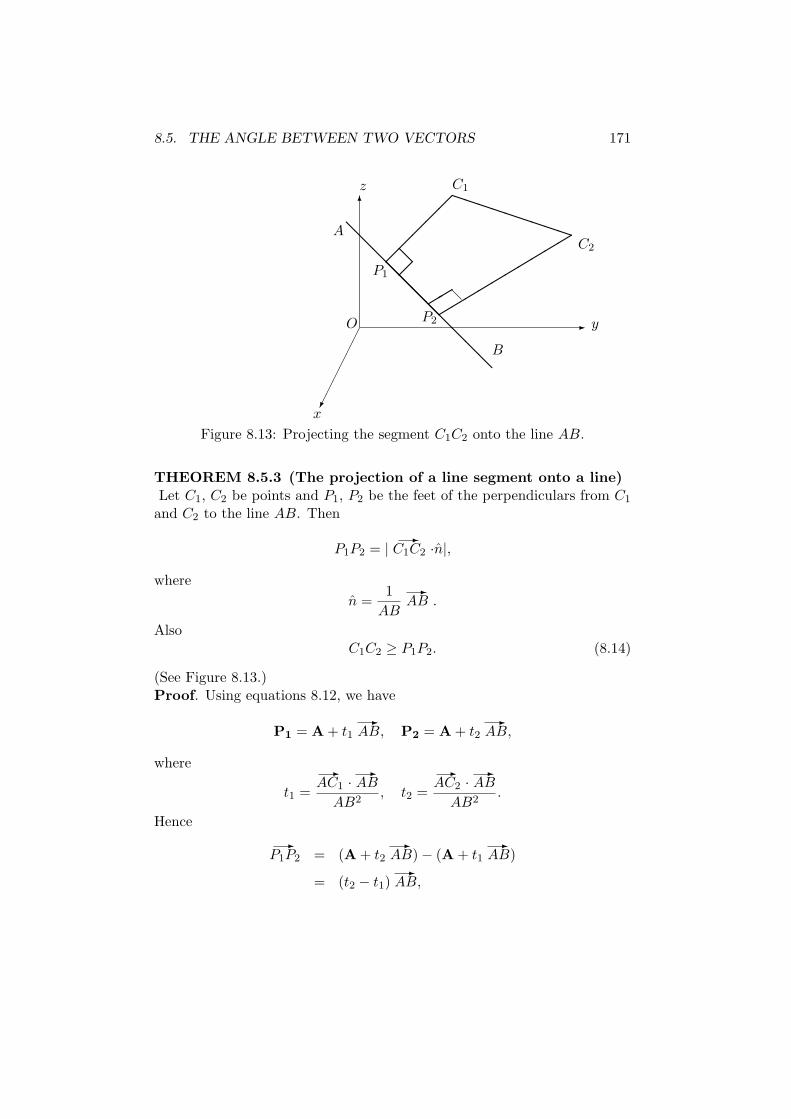
8.5. THE ANGLE BETWEEN TWO VECTORS 171
¢¢
¢¢
¢¢®
-
6
y
z
x
O
@@
@@
@@
@@
@@
@
B
A
¡¡
¡¡
¡
@@
@@""""""""""
PPPPPPPPPC2
C1
P2
P1
@¡
""
Figure 8.13: Projecting the segment C1C2 onto the line AB.
THEOREM 8.5.3 (The projection of a line segment onto a line)Let C1, C2 be points and P1, P2 be the feet of the perpendiculars from C1
and C2 to the line AB. Then
P1P2 = |-
C1C2 ·n|,
where
n =1
AB
-AB .
AlsoC1C2 ≥ P1P2. (8.14)
(See Figure 8.13.)Proof. Using equations 8.12, we have
P1 = A + t1-
AB, P2 = A + t2-
AB,
where
t1 =
-AC1 ·
-AB
AB2, t2 =
-AC2 ·
-AB
AB2.
Hence
-P1P2 = (A + t2
-AB) − (A + t1
-AB)
= (t2 − t1)-
AB,
172 CHAPTER 8. THREE–DIMENSIONAL GEOMETRY
so
P1P2 = ||-
P1P2 || = |t2 − t1|AB
=
∣
∣
∣
∣
∣
∣
-AC2 ·
-AB
AB2−
-AC1 ·
-AB
AB2
∣
∣
∣
∣
∣
∣
AB
=
∣
∣
∣
∣
-C1C2 ·
-AB
∣
∣
∣
∣
AB2AB
=
∣
∣
∣
∣
-C1C2 ·n
∣
∣
∣
∣
,
where n is the unit vector
n =1
AB
-AB .
Inequality 8.14 then follows from the Cauchy–Schwarz inequality 8.3.
DEFINITION 8.5.3 Two non–intersecting lines are called skew if theyhave non–parallel direction vectors.
Theorem 8.5.3 has an application to the problem of showing that two skewlines have a shortest distance between them. (The reader is referred toproblem 16 at the end of the chapter.)
Before we turn to the study of planes, it is convenient to introduce thecross–product of two vectors.
8.6 The cross–product of two vectors
DEFINITION 8.6.1 Let X = a1i + b1j + c1k and Y = a2i + b2j + c2k.Then X × Y , the cross–product of X and Y , is defined by
X × Y = ai + bj + ck,
where
a =
∣
∣
∣
∣
b1 c1
b2 c2
∣
∣
∣
∣
, b = −∣
∣
∣
∣
a1 c1
a2 c2
∣
∣
∣
∣
, c =
∣
∣
∣
∣
a1 b1
a2 b2
∣
∣
∣
∣
.
The vector cross–product has the following properties which follow fromproperties of 2 × 2 and 3 × 3 determinants:
(i) i × j = k, j × k = i, k × i = j;
8.6. THE CROSS–PRODUCT OF TWO VECTORS 173
(ii) X × X = 0;
(iii) Y × X = −X × Y ;
(iv) X × (Y + Z) = X × Y + X × Z;
(v) (tX) × Y = t(X × Y );
(vi) (Scalar triple product formula) if Z = a3i + b3j + c3k, then
X · (Y × Z) =
∣
∣
∣
∣
∣
∣
a1 b1 c1
a2 b2 c2
a3 b3 c3
∣
∣
∣
∣
∣
∣
= (X × Y ) · Z;
(vii) X · (X × Y ) = 0 = Y · (X × Y );
(viii) ||X × Y || =√
||X||2||Y ||2 − (X · Y )2;
(ix) if X and Y are non–zero vectors and θ is the angle between X and Y ,then
||X × Y || = ||X|| · ||Y || sin θ.
(See Figure 8.14.)
From theorem 8.4.3 and the definition of cross–product, it follows thatnon–zero vectors X and Y are parallel if and only if X × Y = 0; hence by(vii), the cross–product of two non–parallel, non–zero vectors X and Y , isa non–zero vector perpendicular to both X and Y .
LEMMA 8.6.1 Let X and Y be non–zero, non–parallel vectors.
(i) Z is a linear combination of X and Y , if and only if Z is perpendicularto X × Y ;
(ii) Z is perpendicular to X and Y , if and only if Z is parallel to X × Y .
Proof. Let X and Y be non–zero, non–parallel vectors. Then
X × Y 6= 0.
Then if X × Y = ai + bj + ck, we have
det [X × Y |X|Y ]t =
∣
∣
∣
∣
∣
∣
a b ca1 b1 c1
a2 b2 c2
∣
∣
∣
∣
∣
∣
= (X × Y ) · (X × Y ) > 0.
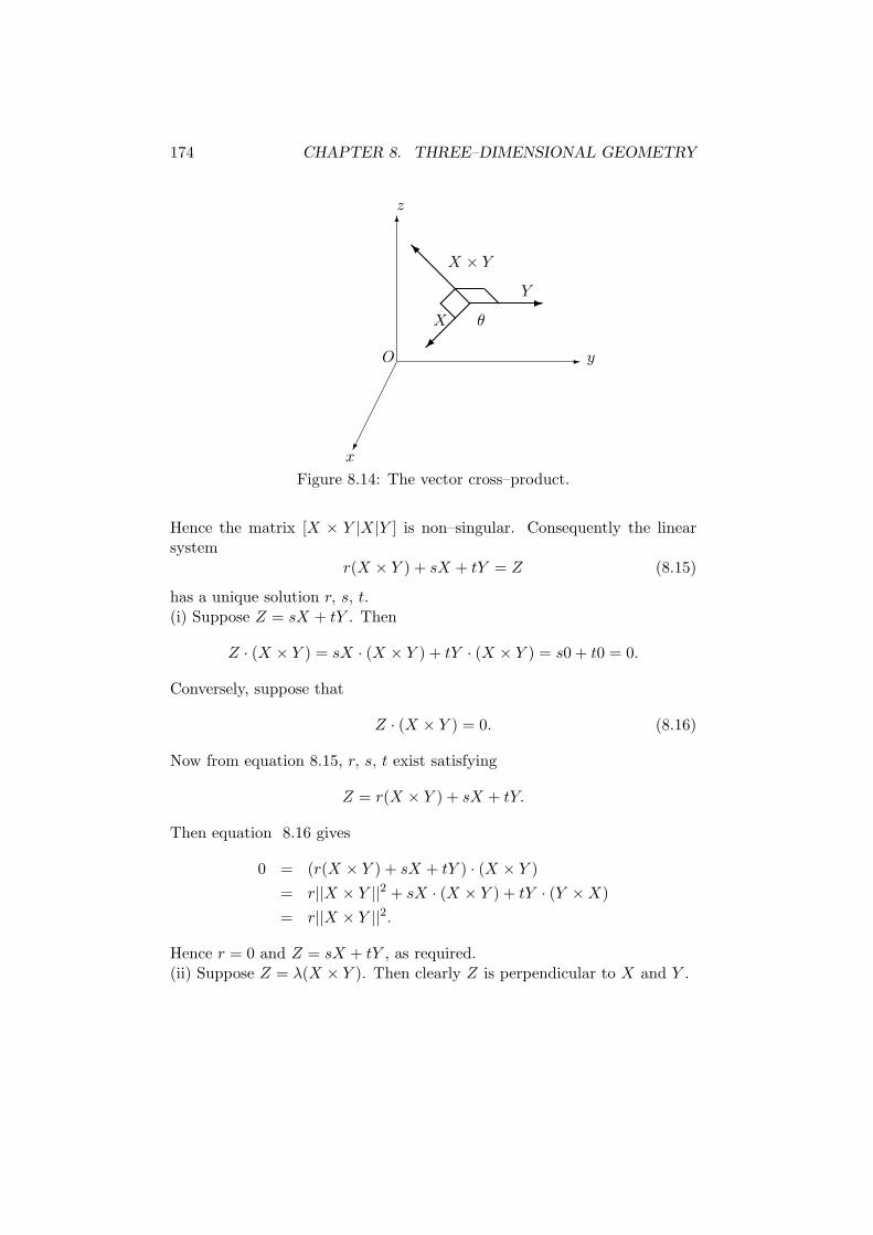
174 CHAPTER 8. THREE–DIMENSIONAL GEOMETRY
¢¢
¢¢
¢¢®
-
6
y
z
x
O
@@
@@I
¡¡
¡ª
-θ
¡ @@X
Y
X × Y
Figure 8.14: The vector cross–product.
Hence the matrix [X × Y |X|Y ] is non–singular. Consequently the linearsystem
r(X × Y ) + sX + tY = Z (8.15)
has a unique solution r, s, t.(i) Suppose Z = sX + tY . Then
Z · (X × Y ) = sX · (X × Y ) + tY · (X × Y ) = s0 + t0 = 0.
Conversely, suppose that
Z · (X × Y ) = 0. (8.16)
Now from equation 8.15, r, s, t exist satisfying
Z = r(X × Y ) + sX + tY.
Then equation 8.16 gives
0 = (r(X × Y ) + sX + tY ) · (X × Y )
= r||X × Y ||2 + sX · (X × Y ) + tY · (Y × X)
= r||X × Y ||2.
Hence r = 0 and Z = sX + tY , as required.(ii) Suppose Z = λ(X × Y ). Then clearly Z is perpendicular to X and Y .
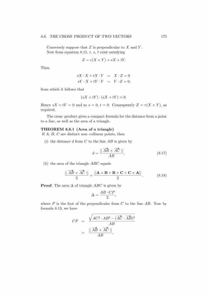
8.6. THE CROSS–PRODUCT OF TWO VECTORS 175
Conversely suppose that Z is perpendicular to X and Y .Now from equation 8.15, r, s, t exist satisfying
Z = r(X × Y ) + sX + tY.
Then
sX · X + tX · Y = X · Z = 0
sY · X + tY · Y = Y · Z = 0,
from which it follows that
(sX + tY ) · (sX + tY ) = 0.
Hence sX + tY = 0 and so s = 0, t = 0. Consequently Z = r(X × Y ), asrequired.
The cross–product gives a compact formula for the distance from a pointto a line, as well as the area of a triangle.
THEOREM 8.6.1 (Area of a triangle)If A, B, C are distinct non–collinear points, then
(i) the distance d from C to the line AB is given by
d =||
-AB ×
-AC ||
AB, (8.17)
(ii) the area of the triangle ABC equals
||-
AB ×-
AC ||2
=||A × B + B × C + C × A||
2. (8.18)
Proof. The area ∆ of triangle ABC is given by
∆ =AB · CP
2,
where P is the foot of the perpendicular from C to the line AB. Now byformula 8.13, we have
CP =
√
AC2 · AB2 − (-
AC ·-
AB)2
AB
=||
-AB ×
-AC ||
AB,
176 CHAPTER 8. THREE–DIMENSIONAL GEOMETRY
which, by property (viii) of the cross–product, gives formula 8.17. Thesecond formula of equation 8.18 follows from the equations
-AB ×
-AC = (B − A) × (C − A)
= {(B − A) × C} − {(C − A) × A}= {(B × C − A × C)} − {(B × A − A × A)}= B × C − A × C − B × A
= B × C + C × A + A × B,
as required.
8.7 Planes
DEFINITION 8.7.1 A plane is a set of points P satisfying an equationof the form
P = P0 + sX + tY, s, t ∈ R, (8.19)
where X and Y are non–zero, non–parallel vectors.
For example, the xy–plane consists of the points P = (x, y, 0) and corre-sponds to the plane equation
P = xi + yj = O + xi + yj.
In terms of coordinates, equation 8.19 takes the form
x = x0 + sa1 + ta2
y = y0 + sb1 + tb2
z = z0 + sc1 + tc2,
where P0 = (x0, y0, z0) and (a1, b1, c1) and (a2, b2, c2) are non–zero andnon–proportional.
THEOREM 8.7.1 Let A, B, C be three non–collinear points. Then thereis one and only one plane through these points, namely the plane given bythe equation
P = A + s-
AB +t-
AC, (8.20)
or equivalently-
AP= s-
AB +t-
AC . (8.21)
(See Figure 8.15.)
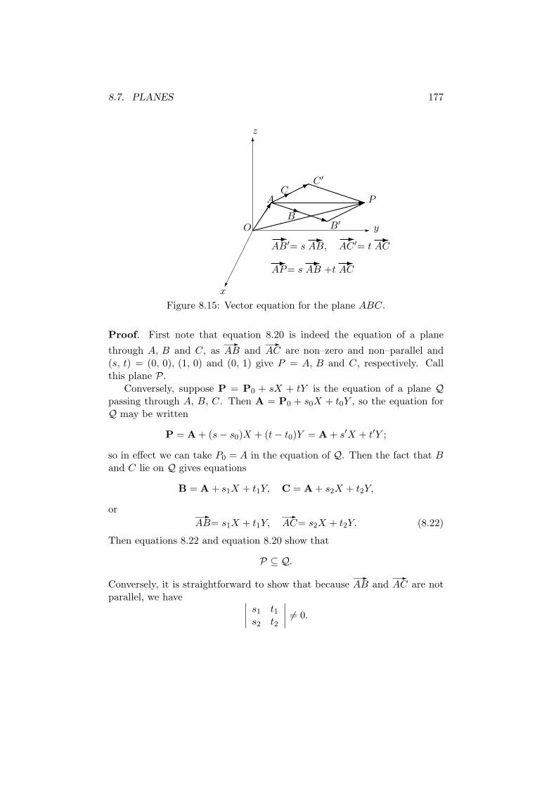
8.7. PLANES 177
¢¢
¢¢
¢¢®
-
6
y
z
x
O»»»»»»»»»»»»:
Á©©©©*
-PPPPPPq
PPPPPP
©©©©*
qA
C
BB′
C ′
P
-AB′= s
-AB,
-AC ′= t
-AC
-AP= s
-AB +t
-AC
Figure 8.15: Vector equation for the plane ABC.
Proof. First note that equation 8.20 is indeed the equation of a plane
through A, B and C, as-
AB and-
AC are non–zero and non–parallel and(s, t) = (0, 0), (1, 0) and (0, 1) give P = A, B and C, respectively. Callthis plane P.
Conversely, suppose P = P0 + sX + tY is the equation of a plane Qpassing through A, B, C. Then A = P0 + s0X + t0Y , so the equation forQ may be written
P = A + (s − s0)X + (t − t0)Y = A + s′X + t′Y ;
so in effect we can take P0 = A in the equation of Q. Then the fact that Band C lie on Q gives equations
B = A + s1X + t1Y, C = A + s2X + t2Y,
or -AB= s1X + t1Y,
-AC= s2X + t2Y. (8.22)
Then equations 8.22 and equation 8.20 show that
P ⊆ Q.
Conversely, it is straightforward to show that because-
AB and-
AC are notparallel, we have
∣
∣
∣
∣
s1 t1s2 t2
∣
∣
∣
∣
6= 0.
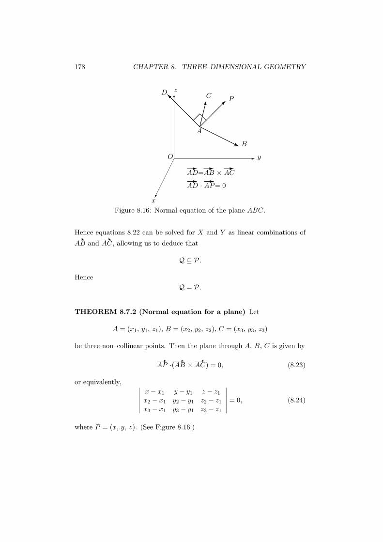
178 CHAPTER 8. THREE–DIMENSIONAL GEOMETRY
¢¢
¢¢
¢¢®
-
6
y
z
x
O
@@
@@
@I
¤¤¤¤º
¡¡
¡¡µ
HHHHHHj
@¡
A
B
C PD
-AD=
-AB ×
-AC
-AD ·
-AP= 0
Figure 8.16: Normal equation of the plane ABC.
Hence equations 8.22 can be solved for X and Y as linear combinations of-
AB and-
AC, allowing us to deduce that
Q ⊆ P.
Hence
Q = P.
THEOREM 8.7.2 (Normal equation for a plane) Let
A = (x1, y1, z1), B = (x2, y2, z2), C = (x3, y3, z3)
be three non–collinear points. Then the plane through A, B, C is given by
-AP ·(
-AB ×
-AC) = 0, (8.23)
or equivalently,∣
∣
∣
∣
∣
∣
x − x1 y − y1 z − z1
x2 − x1 y2 − y1 z2 − z1
x3 − x1 y3 − y1 z3 − z1
∣
∣
∣
∣
∣
∣
= 0, (8.24)
where P = (x, y, z). (See Figure 8.16.)

8.7. PLANES 179
¢¢
¢¢
¢¢®
-
6
y
z
x
O
¢¢¢¢
¢¢¢¢
»»»»»»»»
»»»»»»»»
AA
AAK ai + bj + ck
ax + by + cz = d
Figure 8.17: The plane ax + by + cz = d.
REMARK 8.7.1 Equation 8.24 can be written in more symmetrical formas
∣
∣
∣
∣
∣
∣
∣
∣
x y z 1x1 y1 z1 1x2 y2 z2 1x3 y3 z3 1
∣
∣
∣
∣
∣
∣
∣
∣
= 0. (8.25)
Proof. Let P be the plane through A, B, C. Then by equation 8.21, we
have P ∈ P if and only if-
AP is a linear combination of-
AB and-
AC and so
by lemma 8.6.1(i), using the fact that-
AB ×-
AC 6= 0 here, if and only if-
AP
is perpendicular to-
AB ×-
AC. This gives equation 8.23.
Equation 8.24 is the scalar triple product version of equation 8.23, takinginto account the equations
-AP = (x − x1)i + (y − y1)j + (z − z1)k,-
AB = (x2 − x1)i + (y2 − y1)j + (z2 − z1)k,-
AC = (x3 − x1)i + (y3 − y1)j + (z3 − z1)k.
REMARK 8.7.2 Equation 8.24 gives rise to a linear equation in x, y andz:
ax + by + cz = d,

180 CHAPTER 8. THREE–DIMENSIONAL GEOMETRY
where ai + bj + ck 6= 0. For∣
∣
∣
∣
∣
∣
x − x1 y − y1 z − z1
x2 − x1 y2 − y1 z2 − z1
x3 − x1 y3 − y1 z3 − z1
∣
∣
∣
∣
∣
∣
=
∣
∣
∣
∣
∣
∣
x y zx2 − x1 y2 − y1 z2 − z1
x3 − x1 y3 − y1 z3 − z1
∣
∣
∣
∣
∣
∣
−
∣
∣
∣
∣
∣
∣
x1 y1 z1
x2 − x1 y2 − y1 z2 − z1
x3 − x1 y3 − y1 z3 − z1
∣
∣
∣
∣
∣
∣
(8.26)
and expanding the first determinant on the right–hand side of equation 8.26along row 1 gives an expression
ax + by + cz
where
a =
˛
˛
˛
˛
y2 − y1 z2 − z1
y3 − y1 z3 − z1
˛
˛
˛
˛
, b = −˛
˛
˛
˛
x2 − x1 z2 − z1
x3 − x1 z3 − z1
˛
˛
˛
˛
, c =
˛
˛
˛
˛
x2 − x1 y2 − y1
x3 − x1 y3 − y1
˛
˛
˛
˛
.
But a, b, c are the components of-
AB ×-
AC, which in turn is non–zero, asA, B, C are non–collinear here.
Conversely if ai + bj + ck 6= 0, the equation
ax + by + cz = d
does indeed represent a plane. For if say a 6= 0, the equation can be solvedfor x in terms of y and z:
xyz
=
−da00
+ y
− ba10
+ z
− ca01
,
which gives the planeP = P0 + yX + zY,
where P0 = (−da , 0, 0) and X = − b
a i + j and Y = − ca i + k are evidently
non–parallel vectors.
REMARK 8.7.3 The plane equation ax+by+cz = d is called the normal
form, as it is easy to prove that if P1 and P2 are two points in the plane,
then ai + bj + ck is perpendicular to-
P1P2. Any non–zero vector with thisproperty is called a normal to the plane. (See Figure 8.17.)
By lemma 8.6.1(ii), it follows that every vector X normal to a plane
through three non–collinear points A, B, C is parallel to-
AB ×-
AC, since
X is perpendicular to-
AB and-
AC.
8.7. PLANES 181
EXAMPLE 8.7.1 Show that the planes
x + y − 2z = 1 and x + 3y − z = 4
intersect in a line and find the distance from the point C = (1, 0, 1) to thisline.
Solution. Solving the two equations simultaneously gives
x = −1
2+
5
2z, y =
3
2− 1
2z, (8.27)
where z is arbitrary. Hence
xi + yj + zk = −1
2i − 3
2j + z(
5
2i − 1
2j + k),
which is the equation of a line L through A = (−12 , −3
2 , 0) and havingdirection vector 5
2 i − 12 j + k.
We can now proceed in one of three ways to find the closest point on Lto A.
One way is to use equation 8.17 with B defined by
-AB=
5
2i − 1
2j + k.
Another method minimizes the distance CP , where P ranges over L.A third way is to find an equation for the plane through C, having
52 i − 1
2 j + k as a normal. Such a plane has equation
5x − y + 2z = d,
where d is found by substituting the coordinates of C in the last equation.
d = 5 × 1 − 0 + 2 × 1 = 7.
We now find the point P where the plane intersects the line L. Then-
CPwill be perpendicular to L and CP will be the required shortest distancefrom C to L. We find using equations 8.27 that
5(−1
2+
5
2z) − (
3
2− 1
2z) + 2z = 7,
so z = 1115 . Hence P = (4
3 , 1715 , 11
15).
It is clear that through a given line and a point not on that line, therepasses exactly one plane. If the line is given as the intersection of two planes,each in normal form, there is a simple way of finding an equation for thisplane. More explicitly we have the following result:
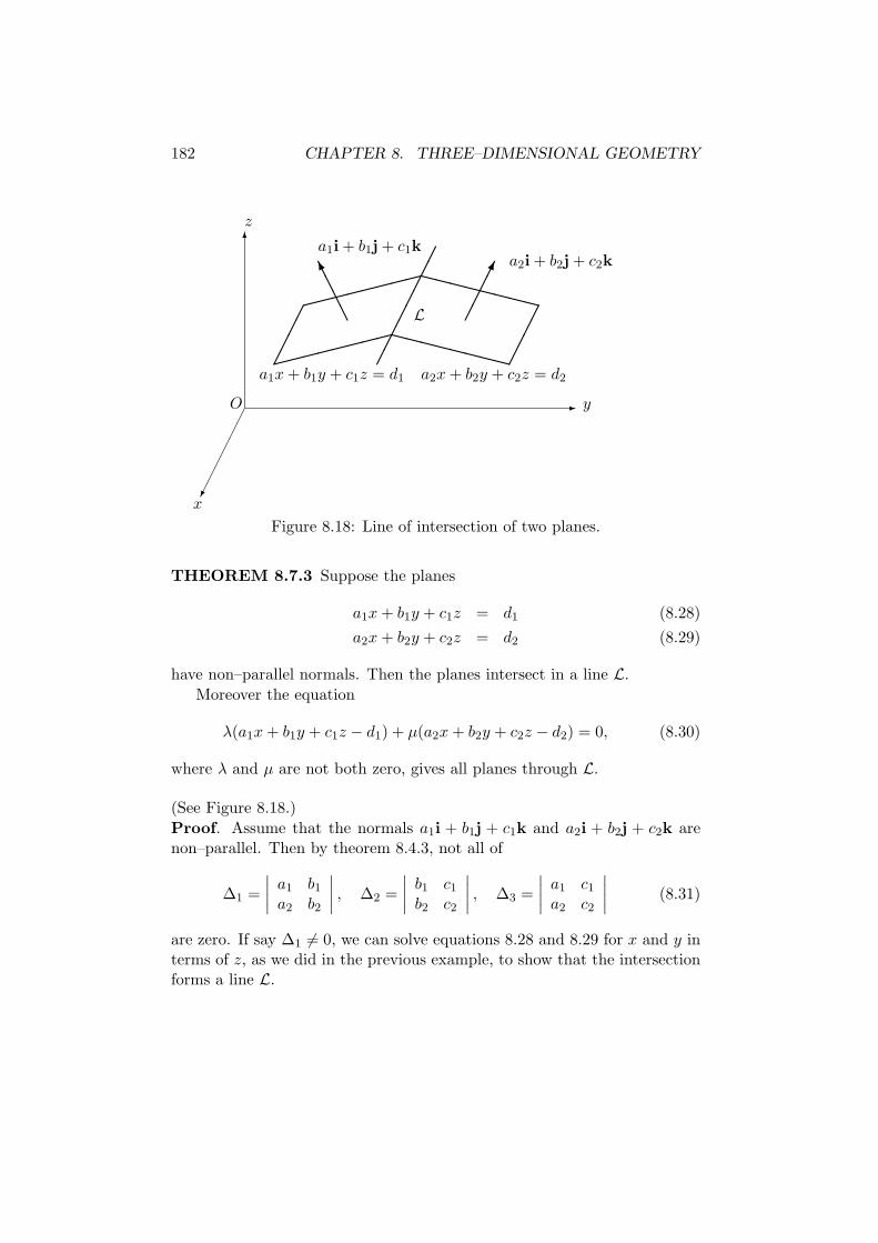
182 CHAPTER 8. THREE–DIMENSIONAL GEOMETRY
¢¢
¢¢
¢¢®
-
6
y
z
x
O
¢¢¢¢
¢¢¢¢¢¢¢¢
»»»»»»»»
»»»»»»»»
AA
AAK
a1i + b1j + c1ka2i + b2j + c2k
a1x + b1y + c1z = d1 a2x + b2y + c2z = d2
XXXXXXXX
XXXXXXXX
¢¢¢¢¢
¢¢¢
L
Figure 8.18: Line of intersection of two planes.
THEOREM 8.7.3 Suppose the planes
a1x + b1y + c1z = d1 (8.28)
a2x + b2y + c2z = d2 (8.29)
have non–parallel normals. Then the planes intersect in a line L.
Moreover the equation
λ(a1x + b1y + c1z − d1) + µ(a2x + b2y + c2z − d2) = 0, (8.30)
where λ and µ are not both zero, gives all planes through L.
(See Figure 8.18.)
Proof. Assume that the normals a1i + b1j + c1k and a2i + b2j + c2k arenon–parallel. Then by theorem 8.4.3, not all of
∆1 =
∣
∣
∣
∣
a1 b1
a2 b2
∣
∣
∣
∣
, ∆2 =
∣
∣
∣
∣
b1 c1
b2 c2
∣
∣
∣
∣
, ∆3 =
∣
∣
∣
∣
a1 c1
a2 c2
∣
∣
∣
∣
(8.31)
are zero. If say ∆1 6= 0, we can solve equations 8.28 and 8.29 for x and y interms of z, as we did in the previous example, to show that the intersectionforms a line L.
8.7. PLANES 183
We next have to check that if λ and µ are not both zero, then equa-tion 8.30 represents a plane. (Whatever set of points equation 8.30 repre-sents, this set certainly contains L.)
(λa1 + µa2)x + (λb1 + µb2)y + (λc1 + µc2)z − (λd1 + µd2) = 0.
Then we clearly cannot have all the coefficients
λa1 + µa2, λb1 + µb2, λc1 + µc2
zero, as otherwise the vectors a1i + b1j + c1k and a2i + b2j + c2k would beparallel.
Finally, if P is a plane containing L, let P0 = (x0, y0, z0) be a point noton L. Then if we define λ and µ by
λ = −(a2x0 + b2y0 + c2z0 − d2), µ = a1x0 + b1y0 + c1z0 − d1,
then at least one of λ and µ is non–zero. Then the coordinates of P0 satisfyequation 8.30, which therefore represents a plane passing through L and P0
and hence identical with P.
EXAMPLE 8.7.2 Find an equation for the plane through P0 = (1, 0, 1)and passing through the line of intersection of the planes
x + y − 2z = 1 and x + 3y − z = 4.
Solution. The required plane has the form
λ(x + y − 2z − 1) + µ(x + 3y − z − 4) = 0,
where not both of λ and µ are zero. Substituting the coordinates of P0 intothis equation gives
−2λ + µ(−4) = 0, λ = −2µ.
So the required equation is
−2µ(x + y − 2z − 1) + µ(x + 3y − z − 4) = 0,
or−x + y + 3z − 2 = 0.
Our final result is a formula for the distance from a point to a plane.
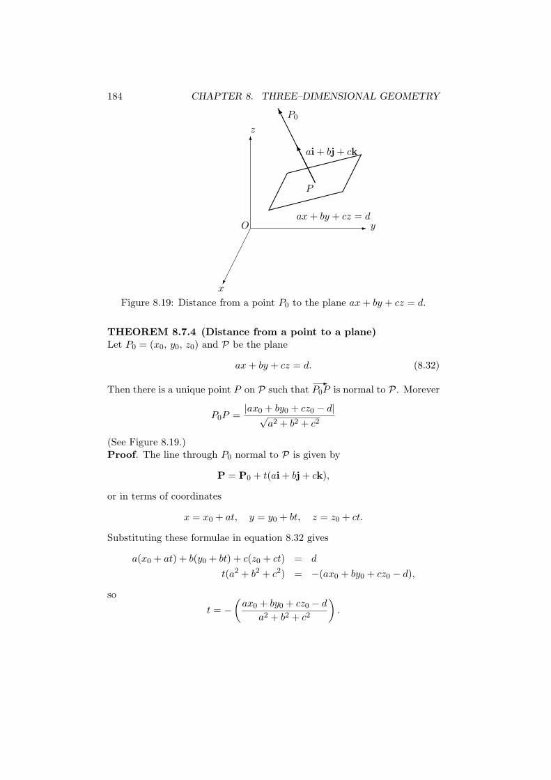
184 CHAPTER 8. THREE–DIMENSIONAL GEOMETRY
¢¢
¢¢
¢¢®
-
6
y
z
x
O
¢¢¢¢
¢¢¢¢
»»»»»»»»
»»»»»»»»
AA
AAK
AA
AA
AA
AAK
ai + bj + ck
ax + by + cz = d
P0
P
Figure 8.19: Distance from a point P0 to the plane ax + by + cz = d.
THEOREM 8.7.4 (Distance from a point to a plane)Let P0 = (x0, y0, z0) and P be the plane
ax + by + cz = d. (8.32)
Then there is a unique point P on P such that-
P0P is normal to P. Morever
P0P =|ax0 + by0 + cz0 − d|√
a2 + b2 + c2
(See Figure 8.19.)Proof. The line through P0 normal to P is given by
P = P0 + t(ai + bj + ck),
or in terms of coordinates
x = x0 + at, y = y0 + bt, z = z0 + ct.
Substituting these formulae in equation 8.32 gives
a(x0 + at) + b(y0 + bt) + c(z0 + ct) = d
t(a2 + b2 + c2) = −(ax0 + by0 + cz0 − d),
so
t = −(
ax0 + by0 + cz0 − d
a2 + b2 + c2
)
.
8.8. PROBLEMS 185
Then
P0P = ||-
P0P || = ||t(ai + bj + ck)||= |t|
√
a2 + b2 + c2
=|ax0 + by0 + cz0 − d|
a2 + b2 + c2
√
a2 + b2 + c2
=|ax0 + by0 + cz0 − d|√
a2 + b2 + c2.
Other interesting geometrical facts about lines and planes are left to theproblems at the end of this chapter.
8.8 PROBLEMS
.
1. Find the point where the line through A = (3, −2, 7) and B =(13, 3, −8) meets the xz–plane.
[Ans: (7, 0, 1).]
2. Let A, B, C be non–collinear points. If E is the mid–point of thesegment BC and F is the point on the segment EA satisfying AF
EF = 2,prove that
F =1
3(A + B + C).
(F is called the centroid of triangle ABC.)
3. Prove that the points (2, 1, 4), (1, −1, 2), (3, 3, 6) are collinear.
4. If A = (2, 3, −1) and B = (3, 7, 4), find the points P on the line ABsatisfying PA/PB = 2/5.
[Ans:(
167 , 29
7 , 37
)
and(
43 , 1
3 , −133
)
.]
5. Let M be the line through A = (1, 2, 3) parallel to the line joiningB = (−2, 2, 0) and C = (4, −1, 7). Also N is the line joining E =(1, −1, 8) and F = (10, −1, 11). Prove that M and N intersect andfind the point of intersection.
[Ans: (7, −1, 10).]
186 CHAPTER 8. THREE–DIMENSIONAL GEOMETRY
6. Prove that the triangle formed by the points (−3, 5, 6), (−2, 7, 9) and(2, 1, 7) is a 30o, 60o, 90o triangle.
7. Find the point on the line AB closest to the origin, where A =(−2, 1, 3) and B = (1, 2, 4). Also find this shortest distance.
[Ans:(
−1611 , 13
11 , 3511
)
and√
15011 .]
8. A line N is determined by the two planes
x + y − 2z = 1, and x + 3y − z = 4.
Find the point P on N closest to the point C = (1, 0, 1) and find thedistance PC.
[Ans:(
43 , 17
15 , 1115
)
and√
33015 .]
9. Find a linear equation describing the plane perpendicular to the lineof intersection of the planes x + y − 2z = 4 and 3x − 2y + z = 1 andwhich passes through (6, 0, 2).
[Ans: 3x + 7y + 5z = 28.]
10. Find the length of the projection of the segment AB on the line L,where A = (1, 2, 3), B = (5, −2, 6) and L is the line CD, whereC = (7, 1, 9) and D = (−1, 5, 8).
[Ans: 173 .]
11. Find a linear equation for the plane through A = (3, −1, 2), perpen-dicular to the line L joining B = (2, 1, 4) and C = (−3, −1, 7). Alsofind the point of intersection of L and the plane and hence determine
the distance from A to L. [Ans: 5x+2y−3z = 7,(
11138 , 52
38 , 13138
)
,√
29338 .]
12. If P is a point inside the triangle ABC, prove that
P = rA + sB + tC,
where r + s + t = 1 and r > 0, s > 0, t > 0.
13. If B is the point where the perpendicular from A = (6, −1, 11) meetsthe plane 3x + 4y + 5z = 10, find B and the distance AB.
[Ans: B =(
12350 , −286
50 , 25550
)
and AB = 59√50
.]
8.8. PROBLEMS 187
14. Prove that the triangle with vertices (−3, 0, 2), (6, 1, 4), (−5, 1, 0)has area 1
2
√333.
15. Find an equation for the plane through (2, 1, 4), (1, −1, 2), (4, −1, 1).
[Ans: 2x − 7y + 6z = 21.]
16. Lines L and M are non–parallel in 3–dimensional space and are givenby equations
P = A + sX, Q = B + tY.
(i) Prove that there is precisely one pair of points P and Q such that-
PQ is perpendicular to X and Y .
(ii) Explain why PQ is the shortest distance between lines L and M.
Also prove that
PQ =| (X × Y )·
-AB|
‖X × Y ‖ .
17. If L is the line through A = (1, 2, 1) and C = (3, −1, 2), while Mis the line through B = (1, 0, 2) and D = (2, 1, 3), prove that theshortest distance between L and M equals 13√
62.
18. Prove that the volume of the tetrahedron formed by four non–coplanarpoints Ai = (xi, yi, zi), 1 ≤ i ≤ 4, is equal to
1
6| (
-A1A2 ×
-A1A3)·
-A1A4|,
which in turn equals the absolute value of the determinant
1
6
∣
∣
∣
∣
∣
∣
∣
∣
1 x1 y1 z1
1 x2 y2 z2
1 x3 y3 z3
1 x4 y4 z4
∣
∣
∣
∣
∣
∣
∣
∣
.
19. The points A = (1, 1, 5), B = (2, 2, 1), C = (1, −2, 2) and D =(−2, 1, 2) are the vertices of a tetrahedron. Find the equation of theline through A perpendicular to the face BCD and the distance of Afrom this face. Also find the shortest distance between the skew linesAD and BC.
[Ans: P = (1 + t)(i + j + 5k); 2√
3; 3.]

188
Chapter 9
FURTHER READING
Matrix theory has many applications to science, mathematics, economicsand engineering. Some of these applications can be found in the books[2, 3, 4, 5, 11, 13, 16, 20, 26, 28].
For the numerical side of matrix theory, [6] is recommended. Its bibliographyis also useful as a source of further references.
For applications to:
1. Graph theory, see [7, 13];
2. Coding theory, see [8, 15];
3. Game theory, see [13];
4. Statistics, see [9];
5. Economics, see [10];
6. Biological systems, see [12];
7. Markov non–negative matrices, see [11, 13, 14, 17];
8. The general equation of the second degree in three variables, see [18];
9. Affine and projective geometry, see [19, 21, 22];
10. Computer graphics, see [23, 24].
189

190
Bibliography
[1] B. Noble. Applied Linear Algebra, 1969. Prentice Hall, NJ.
[2] B. Noble and J.W. Daniel. Applied Linear Algebra, third edition, 1988.
Prentice Hall, NJ.
[3] R.P. Yantis and R.J. Painter. Elementary Matrix Algebra with Appli-
cation, second edition, 1977. Prindle, Weber and Schmidt, Inc. Boston,Massachusetts.
[4] T.J. Fletcher. Linear Algebra through its Applications, 1972. Van Nos-trand Reinhold Company, New York.
[5] A.R. Magid. Applied Matrix Models, 1984. John Wiley and Sons, NewYork.
[6] D.R. Hill and C.B. Moler. Experiments in Computational Matrix Alge-
bra, 1988. Random House, New York.
[7] N. Deo. Graph Theory with Applications to Engineering and Computer
Science, 1974. Prentice–Hall, N. J.
[8] V. Pless. Introduction to the Theory of Error–Correcting Codes, 1982.
John Wiley and Sons, New York.
[9] F.A. Graybill. Matrices with Applications in Statistics, 1983.
Wadsworth, Belmont Ca.
[10] A.C. Chiang. Fundamental Methods of Mathematical Economics, sec-
ond edition, 1974. McGraw–Hill Book Company, New York.
[11] N.J. Pullman. Matrix Theory and its Applications, 1976. Marcel DekkerInc. New York.
191

[12] J.M. Geramita and N.J. Pullman. An Introduction to the Application
of Nonnegative Matrices to Biological Systems, 1984. Queen’s Papersin Pure and Applied Mathematics 68. Queen’s University, Kingston,Canada.
[13] M. Pearl. Matrix Theory and Finite Mathematics, 1973. McGraw–HillBook Company, New York.
[14] J.G. Kemeny and J.L. Snell. Finite Markov Chains, 1967. Van NostrandReinhold, N.J.
[15] E.R. Berlekamp. Algebraic Coding Theory, 1968. McGraw–Hill BookCompany, New York.
[16] G. Strang. Linear Algebra and its Applications, 1988. Harcourt BraceJovanovich, San Diego.
[17] H. Minc. Nonnegative Matrices, 1988. John Wiley and Sons, New York.
[18] G.C. Preston and A.R. Lovaglia. Modern Analytic Geometry, 1971.
Harper and Row, New York.
[19] J.A. Murtha and E.R. Willard. Linear Algebra and Geometry, 1969.
Holt, Rinehart and Winston, Inc. New York.
[20] L.A. Pipes. Matrix Methods for Engineering, 1963. Prentice–Hall, Inc.N. J.
[21] D. Gans. Transformations and Geometries, 1969. Appleton–Century–Crofts, New York.
[22] J.N. Kapur. Transformation Geometry, 1976. Affiliated East–WestPress, New Delhi.
[23] G.C. Reid. Postscript Language Tutorial and Cookbook, 1988. Addison–Wesley Publishing Company, New York.
[24] D. Hearn and M.P. Baker. Computer Graphics, 1989. Prentice–Hall,Inc. N. J.
[25] C.G. Cullen. Linear Algebra with Applications, 1988. Scott, Foresmanand Company, Glenview, Illinois.
[26] R.E. Larson and B.H. Edwards. Elementary Linear Algebra, 1988. D.C.Heath and Company, Lexington, Massachusetts Toronto.
192

[27] N. Magnenat–Thalman and D. Thalmann. State–of–the–art–in Com-
puter Animation, 1989. Springer–Verlag Tokyo.
[28] W.K. Nicholson. Elementary Linear Algebra, 1990. PWS–Kent, Boston.
193
Index
2 × 2 determinant, 71
algorithm, Gauss-Jordan, 8angle between vectors, 166asymptotes, 137
basis, left-to-right algorithm, 62
Cauchy-Schwarz inequality, 159centroid, 185column space, 56complex number, 89complex number, imaginary number,
90complex number, imaginary part, 89complex number, rationalization, 91complex number, real, 89complex number, real part, 89complex numbers, Apollonius’ circle,
100complex numbers, Argand diagram,
95complex numbers, argument, 103complex numbers, complex conjugate,
96complex numbers, complex exponen-
tial, 106complex numbers, complex plane, 95complex numbers, cross-ratio, 114complex numbers, De Moivre, 107complex numbers, lower half plane,
95complex numbers, modulus, 99
complex numbers, modulus-argumentform, 103
complex numbers, polar representa-tion, 103
complex numbers, ratio formulae, 100
complex numbers, square root, 92
complex numbers, upper half plane,95
coordinate axes, 154
coordinate planes, 154
cosine rule, 166
determinant, 38
determinant, cofactor, 76
determinant, diagonal matrix, 74
determinant, Laplace expansion, 73
determinant, lower triangular, 74
determinant, minor, 72
determinant, recursive definition, 72
determinant, scalar matrix, 74
determinant, Surveyor’s formula, 84
determinant, upper triangular, 74
differential equations, 120
direction of a vector, 164
distance, 154
distance to a plane, 184
dot product, 131, 156
eigenvalue, 118
eigenvalues, characteristic equation,118
eigenvector, 118
194
ellipse, 137equation, linear, 1equations, consistent system of, 1, 11equations, Cramer’s rule, 39equations, dependent unknowns, 11equations, homogeneous system of, 16equations, homogeneous, non–trivial
solution, 16equations, homogeneous, trivial solu-
tion, 16equations, inconsistent system of, 1equations, independent unknowns, 11equations, system of linear, 1
factor theorem, 95field, 3field, additive inverse, 3field, multiplicative inverse, 4
Gauss’ theorem, 95
hyperbola, 137
imaginary axis, 95independence, left-to-right test, 59inversion, 74
Joachimsthal, 163
least squares, 47least squares, normal equations, 47least squares, residuals, 47length of a vector, 131, 157linear combination, 17linear dependence, 58linear equations, Cramer’s rule, 83linear transformation, 27linearly independent, 40
mathematical induction, 31matrices, row–equivalence of, 7matrix, 23
matrix, addition, 23matrix, additive inverse, 24matrix, adjoint, 78matrix, augmented, 2matrix, coefficient, 26matrix, coefficient , 2matrix, diagonal, 49matrix, elementary row, 41matrix, elementary row operations, 7matrix, equality, 23matrix, Gram, 132matrix, identity, 31matrix, inverse, 36matrix, invertible, 36matrix, Markov, 53matrix, non–singular, 36matrix, non–singular diagonal, 49matrix, orthogonal , 130matrix, power, 31matrix, product, 25matrix, proper orthogonal, 130matrix, reduced row–echelon form, 6matrix, row-echelon form, 6matrix, scalar multiple, 24matrix, singular, 36matrix, skew–symmetric, 46matrix, subtraction, 24matrix, symmetric, 46matrix, transpose, 45matrix, unit vectors, 28matrix, zero, 24modular addition, 4modular multiplication, 4
normal form, 180
orthogonal matrix, 116orthogonal vectors, 168
parabola, 137parallel lines, 164
195
parallelogram law, 150perpendicular vectors, 168plane, 176plane through 3 points, 176, 178position vector, 156positive octant, 154projection on a line, 171
rank, 65real axis, 95recurrence relations, 32reflection equations, 29rotation equations, 28row space, 56
scalar multiplication of vectors, 150scalar triple product, 173skew lines, 172subspace, 55subspace, basis, 61subspace, dimension, 63subspace, generated, 56subspace, null space, 55
Three–dimensional space, 154triangle inequality, 160
unit vectors, 158
vector cross-product, 172vector equality, 149, 165vector, column, 27vector, of constants, 26vector, of unknowns, 26vectors, parallel vectors, 164
196