elemental analysis of thin layers byx-rays bound... · elemental analysis of thin layers by x-rays...

Philips J. Res. 47 (1993) 247-262

ELEMENTAL ANALYSIS OF THINLAYERS BY X-RAYS

by PETER VAN DE WEIJER and DICK K.G. DE BOERPhilips Research Laboratories, PiO, Box 80000, 5600 JA Eindhoven, The Netherlands

AbstractThe interaction of X-rays with atoms in thin-layer samples can be used todetermine the composition and thickness of the layer. X-Ray fluorescenceis a fast and precise method of determining these parameters for relativelysimple (multi-)layers. For more complex multilayers, glancing incidenceX-ray analysis (a combination offiuorescence, diffraction and reflection) isa promising method of solving the analytical problem.Keywords: elemental analysis, glancing-incidence X-ray analysis, thin

layer, X-ray fluorescence.

Philips Journal of Research Vol.47 Nos.3-5 1993 247

1. Introduetion

In modern technology thin films are used in a variety of applications fortheir mechanical, magnetic, optical and/or electrical properties. These proper-ties are related to the elemental composition and the thickness of the thinlayers. The determination of these parameters in relation to those propertiesis essential for the research and development of new thin film applications.This paper deals with the determination of the elemental composition andthickness of thin films, based on the interaction of the thin-film material withX-rays. Firstly, we describe the analysis of layers with X-ray fluorescence(XRF), based on a commercially available wavelength-dispersive X-rayfluorescence spectrometer. Secondly, a description is given of a more sophis-ticated technique, glancing-incidence X-ray analysis (GIXA), which combinesXRF, X-ray diffraction and X-ray reflectometry for the analysis of (multi)-layered structures.

P. van de Weijer and D.K.G. de Boer

i2.500

~ 2.000o-'"

1.500

1.000

0.500

ZrKA

PbLB

PbLA

0.000 1-__ -'-__ ...L. __ LL__ _1.__ -L1 J...__....L.-l

0.050

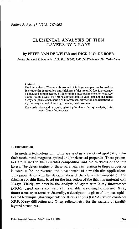
Fig. I. Example of an XRF spectrum. The sample is a layer of PhZr, Ti,_.,O) on platinatedSi02-Si substrates with a thin Ti adhesion layer (see applications below). The continuum is causedby scattering of radiation from the X-ray tube on the sample. The wavelength of the lines arecharacteristic for the elements in the sample.

2. X-ray fluorescence

2.1. Principle

The basic principles ofXRF are described extensively in many textbooks':"),When atoms are irradiated with X-rays, core electrons can be ejected fromthose atoms. The resulting hole can be filled by a transition of an electron froman outer shell. The energy release during that process can be used to eject asecond electron (Auger process) or it can be converted into an X-ray photon(XRF). For inner-shell transitions of heavyelements XRF is the dominantprocess, whereas for outer-shell processes the Auger process is dominant. Thisis one ofthe reasons for the relatively low sensitivity ofXRF for light elements.The energy of the emitted photons in XRF corresponds to the energy differ-ence between the atomic states. As a result this energy, and the correspondingwavelength, is characteristic for the atom under consideration. An example ofan XRF spectrum is given in fig. 1. The fluorescence wavelength varies from0.01 nm for inner-shell transitions in heavyelements to 10nm for lightelements or transitions in the outer shells. The intensity of the XRF signal isa measure for the concentration ofthe element under consideration. However,it also depends on the concentration of the other elements in the sample(matrix), which can complicate the quantification (see below).

248

0.060 0.070 0.080 0.090 0.100 0.1200.110

wavelength (nrn) -

Phllips Journal of Research Vol.47 Nos. 3-5 1993

Elemental analysis of thin layers by X-rays

Crystal changer

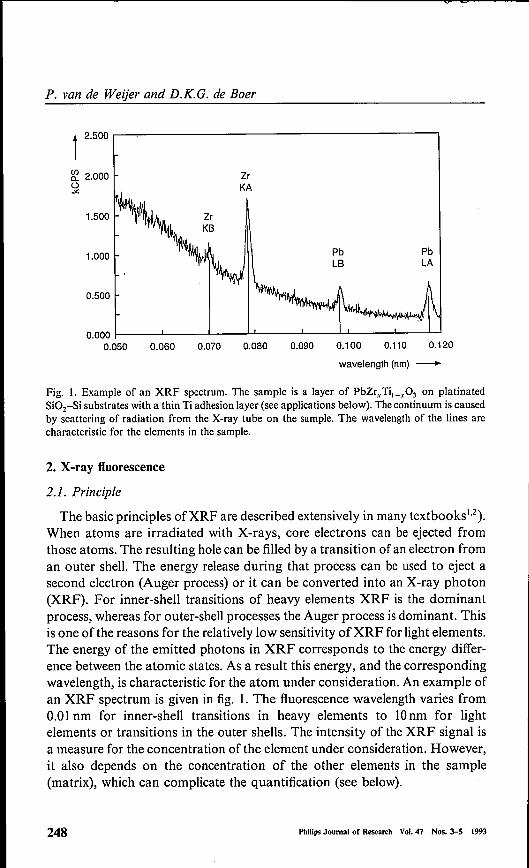
Fig. 2. Schematic diagram of a wavelength-dispersive XRF spectrometer,

2.2. Instrument

An XRF instrument consists of three main parts: an X-ray source to inducethe fluorescence, a dispersive element to separate fluorescence from differentatoms and a detector. For the analyses reported here, we use a Philips 1404sequential spectrometer. It consists of a hot-cathode side-window X-ray tubewith chromium anode as the X-ray source, a monochromator, equipped withseveral Bragg diffractors for the different wavelength intervals, and two detec-tors, a gas-flow detector and a scintillation counter, which can be usedseparately or in tandem. A diagram of the spectrometer is given in fig. 2.

2.3. Quantification

Traditionally XRF is used as a relative technique. This means that calibra-tion standards in the composition range of interest are required to transposethe peak intensities into absolute compositions/thicknesses. The quantificationis performed using empirical calibration functions. For simple applications,e.g. bulk analysis with small variation in the elemental composition, straightline calibration functions are sufficient. For large compositional ranges, matrixeffects (X-ray absorption, fluorescence enhancement, inter-layer effects) resultin a concentration dependent slope of the calibration line. Quantification withfundamental parameters') allows XRF to be used as an absolute technique,provided that the instrumental factors (transmission and detection efficiency ofthe spectrometer) are known. In general, these factors are easily obtained fromthe pure elements. With these factors the intensity of any XRF line from asample ofknown composition can be calculated from fundamental parameters(fluorescence yields, absorption coefficients and tube spectra). This approach

PhiUps Journal of Research Vol. 47 Nos.3-5 1993 249

250 Philips JournnI of Research Vol.47 Nos. 3-5 1993


can also be applied to calculate the composition of an unknown sample fromits measured intensities. In this procedure the measured intensities are used tomake a rough estimate of the composition. Then, by iteration, the actualcomposition is determined. For thin layer analysis the fundamental parameterapproach is the obvious way since calibration standards with similar com-position and thickness are usually not available. The fundamental parameterapproach is fast and inexpensive compared to the traditional calibrationprocedure. Our fundamental parameter approach (FPMULTI)3,4) calculatesfluorescence for K- and L-lines on basis of excitation by primary and secon-dary X-rays, including interlayer effects"). Fluorescence for M-lines, excitationby photoelectrons and by tertiary X-rays are not taken into account.

2.4. Performance

With this XRF spectrometer, elemental information is obtained in the rangefrom boron to uranium. XRF is a surface sensitive technique. The informationdepth is governed by the escape depth of the fluorescence radiation. It variesbetween 100nm for soft X-rays and 100.um for hard X-rays. Therefore, it isessential for the interpretation of the XRF analysis of bulk materials that thecomposition of the bulk is the same as the composition of the probed top layer.Furthermore, owing to the restricted information depth, the detection limit forbulk analysis (~ 1 ppm) is relatively poor in comparison to many othertechniques which can be used for elemental analysis. For thin-layer analysis,however, the information depth concerns the full layer thickness or, at least,is a substantial part of it. As a result, detection limits of XRF for thin-layeranalyses (~ 0.1 monolayer) can compete with those of many other techniquesused for this purpose. The precision of XRF is generally determined by thecounting statistical error and the instrumental stability; a precision of 0.5% isreadily obtainable. The accuracy ofXRF is primarily determined by the errorsin the quantification method. With traditional calibration methods the accu-racy is usually determined by possible errors in the chemical composition ofthe calibration standards and the fit of the emperical calibration function.With the fundamental parameter method, the accuracy depends on the com-pleteness ofthe model, the uncertainties in the fundamental parameters and inthe description of the sample. The accuracy is not known in advance when anew application is set up, it must be determined by an independent referenceanalysis for which the (high) accuracy is known. In our experience the accuracyof the XRF results when using FPMUL TI is typically 2-5%. The applicationof the fundamental parameter approach in combination with the naturalgeometry of thin-layer samples, which permit XRF analysis without any

Philips Journalof Research Vol.47 Nos. 3-5 1993 251


sample preparation, results in a large sample throughput. In 1992 we analysedmore than 4000 samples with a large variety in composition. 90% of thesesamples were thin-layer samples. The analysis by XRF is non-destructive. Forsome materials, however, radiation damage occurs. Furthermore the sampleshould fit into our sample cup (with dimensions ofbetween 10 and 50mm). Adrawback of the thin-layer analysis with our XRF instrument is the very poorlateral resolution obtained. The smallest sample spot has a diameter of 6mm.For the analysis it must be assumed that the sample is homogeneous over thispart of the sample.

2.5. Applications

In previous publications=:") we described some examples of XRF analysesof thin layers. Here, we present some recent applications, in which the perfor-mance is clearly demonstrated: (i) the analysis of NiFe layers which are usedfor magnetic recording; (ii) the analysis of GeSbTe layers which can be appliedto phase-change recording; (iii) the analysis of PhZr, Til_.~03 layers whichpotentially can be used in binary memories; (iv) the analysis of AlN layerswhich are used in magneto-optical recording.We use XRF for process control of the production ofNiFe layers. In order

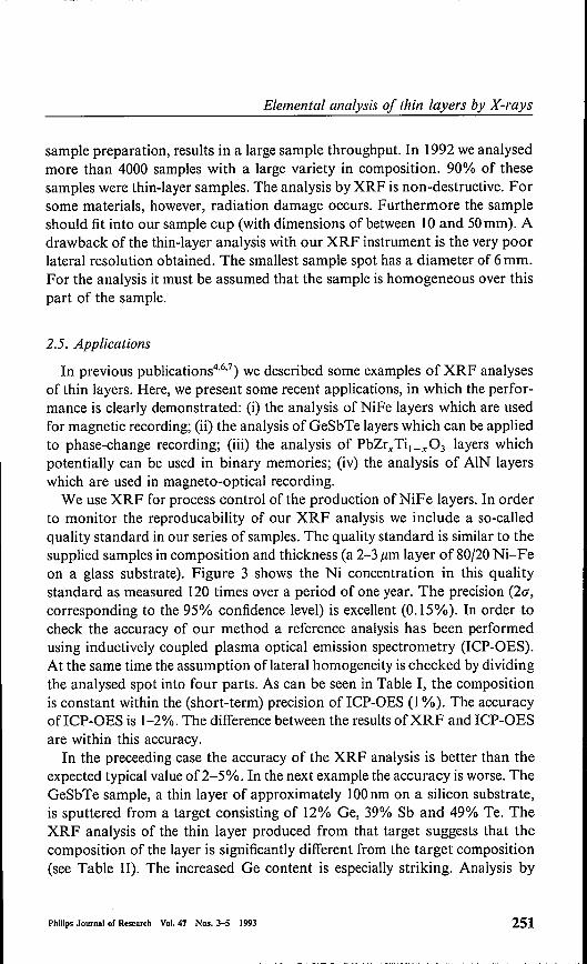
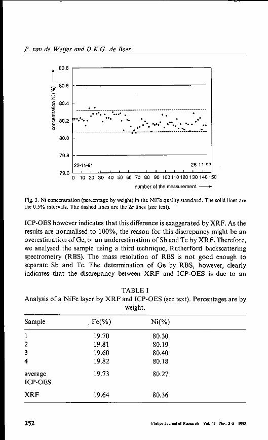
to monitor the reproducability of our XRF analysis we include a so-calledquality standard in our series of samples. The quality standard is similar to thesupplied samples in composition and thickness (a 2-3 Jlm layer of 80/20Ni-Feon a glass substrate). Figure 3 shows the Ni concentration in this qualitystandard as measured 120 times over a period of one year. The precision (20",corresponding to the 95% confidence level) is excellent (0.15%). In order tocheck the accuracy of our method a reference analysis has been performedusing inductively coupled plasma optical emission speetrometry (ICP-OES).At the same time the assumption oflateral homogeneity is checked by dividingthe analysed spot into four parts. As can be seen in Table I, the compositionis constant within the (short-term) precision ofICP-OES (1%). The accuracyofICP-OES is 1-2%. The difference between the results ofXRF and ICP-OESare within this accuracy.In the preceeding case the accuracy of the XRF analysis is better than the

expected typical value of2-5%. In the next example the accuracy is worse. TheGeSbTe sample, a thin layer of approximately 100nm on a silicon substrate,is sputtered from a target consisting of 12% Ge, 39% Sb and 49% Te. TheXRF analysis of the thin layer produced from that target suggests that thecomposition of the layer is significantly different from the target composition(see Table II). The increased Ge content is especially striking. Analysis by


t 80.8

~ 80.6~!!-

79.8

80.0

.§ 80.4~ës 80.2c8

..-------::-;;:-.---.::::--.------------------:-~-------------.------..... . .... .. .... . .. . ..... . ... . .... .. ..... ...-----------------------!.---i!.----------------------------------

22-11-91 26-11-9279.6 L....L-....L--l._J__...J..._....L--l._li__..L-....L--l._l_.l.--'---'

o 10 20 30 40 50 60 70 80 90 100 110 120 130 140 150

number of the measurement -

Fig. 3. Ni concentration (percentage by weight) in the NiFe quality standard. The solid lines arethe 0.5% intervals. The dashed lines are the 2u lines (see text).

Iep-OES however indicates that this difference is exaggerated by XRF. As theresults are normalised to 100%, the reason for this discrepancy might be anoverestimation of Ge, or an underestimation of Sb and Te by XRF. Therefore,we analysed the sample using a third technique, Rutherford backscatteringspeetrometry (RBS). The mass resolution of RBS is not good enough toseparate Sb and Te. The determination of Ge by RBS, however, clearlyindicates that the discrepancy between XRF and Iep-OES is due to an

TABLE IAnalysis of a NiFe layer by XRF and Iep-OES (see text). Percentages are by

weight.

Sample . Fe(%) Ni(%)

19.70 80.302 19.81 80.193 19.60 80.404 19.82 80.18

average 19.73 80.27Iep-OES

XRF 19.64 80.36

252 Philips Journalof Research Vol.47 Nos.3-5 1993

Philips Journalof Research Vol.47 Nos.3-5 1993 253


TABLE IlAnalysis of a GeSbTe thin layer by XRF, lep-OES and RBS. The upper XRFresults are as determined, the lower ones are corrected for the overestimation

of Ge by XRF. Percentages are by number of atoms.

Ge(%) Sb(%) Te(%)

target 12.0 39.0 49.0XRF 14.1 ± 0.2 39.5 ± 0.1 46.5 ± 0.2Iep 12.8 ± 0.2 40.2 ± 0.2 47.0 ± 0.3

XRF(Ge)/RBS(Ge) = 1.120 ± 0.014

XRF 12.8 ± 0.2 40.0 ± 0.5 47.2 ± 0.6

overestimation by XRF of the Ge content by about 10%. This is more thanthe expected typical accuracy of the XRF analysis. Work is in progress toreveal the reason for this discrepancy. It could be due to the fundamentalparameters of Ge itself or to the interaction with Sb and Te.When analysing the Pb'Zr, Til_.,03 samples, layers of approximately 1pm

on platinated Si02-Si substrates with a thin Ti adhesion layer, we do notexpect an acceptable accuracy for the determination of oxygen. The omissionof excitation of oxygen by photoelectrons and by M-lines oflead in FPMUL TIresults in an enormous overestimation of the oxygen content (Table Ill). Theamount of oxygen is calculated to be 4 times the sum of the metal atomswhereas it is expected to be equal to 1.5. The intended implementation of theM-lines in FPMULTI opens the possibility of quantifying light elements, likeoxygen, in samples where the very heavyelements are also present. For thetime being we neglect the oxygen content in the analysis of PhZr, Til_x03

TABLE IIIAnalysis of a Pb.Zr,Til_x03 layer by XRF and lep-OES.

Pb Zr Ti 01017 atoms cm"?

XRF 6.84 3.46 3.04 53.10

O/(Pb + Zr + Ti) = 4.0

XRF 6.82 3.46 3.02Iep 6.90 3.37 3.06

P. van de Weijer and D.K.G. de Boel'

TABLEIVAnalysis of an AlN layer by XRF and wet chemical techniques. Percentages

are by number of atoms.

Al(%) N(%)

XRFWet Chem.

48.049.4

52.050.6

layers. This does not affect the result of the analysis, since oxygen hardlyabsorbs the fluorescence radiation used to quantify the metal atoms: Ph L-line,Zr K-line and Ti K-line. The difference between the XRF and ICP-OES resultsare in the range of the expected typical accuracy of XRF.

Although the quantification of oxygen in the PhZr, Til_x03 layer is not yetpossible using XRF within a reasonable accuracy, this does not mean that thequantification of light elements in thin layers is impossible. This isdemonstrated with the example of AlN sample (IOOnm layer on silicon sub-strates, see Table IV). The low sensitivity of XRF for light elements results ina precision of the nitrogen signalof about 3%. For quantification withFPMULTI the omission of excitation by M-lines is not relevant as such linesare not produced in the layer or the substrate. As a reference analysis thealuminium content of the layer is determined by ICP-OES and the nitrogencontent with ion chromatography. The good agreement with these resultsmight suggest that the contribution of the photoelectrons to the excitation ofnitrogen is relatively unimportant. However, for calibration of the nitrogenXRF signal, we used a SiN thin-layer standard (quantified with RBS). Theneglect of a possibly significant contribution of photoelectrons in the excita-tion of nitrogen is obscured in the result of the analysis as it is expected to besimilar in magnitude for both standard and sample.

3. Glancing incidence X-ray analysis

3.1. Depth profiling with Xi-rays

The afore-mentioned information depth of 100 nm-l 00 !lm for XRF is validfor large incidence and detection angles. In angle-dependent XRF these anglescan be changed and the information depth can be lowered substantially''").

The information depth is as low as a few nanometers in the region of totalreflection. Total reflection can occur if the incidence angle is smaller than theso-called critical angle for total reflection with respect to the sample surface,which is in the order of tenths of a degree. The increased surface sensitivity is

254 Philips Journal of Research Vol. 47 Nos. 3-5 1993


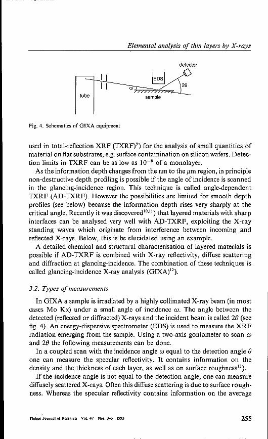
detector

Fig. 4. Schematics of GIXA equipment

used in total-reflection XRF (TXRF)9) for the analysis of small quantities ofmaterialon flat substrates, e.g. surface contamination on silicon wafers. Detec-tion limits in TXRF can be as low as 10-6 of a monolayer.As the information depth changes from the nm to the pm region, in principle

non-destructive depth profiling is possible if the angle of incidence is scannedin the glancing-incidence region. This technique is called angle-dependentTXRF (AD-TXRF). However the possibilities are limited for smooth depthprofiles (see below) because the information depth rises very sharply at thecritical angle. Recently it was discovered'?'!') that layered materials with sharpinterfaces can be analysed very well with AD-TXRF, exploiting the X-raystanding waves which originate from interference between incoming andreflected X-rays. Below, this is be elucidated using an example.A detailed chemical and structural characterisation of layered materials is

possible if AD-TXRF is combined with X-ray reflectivity, diffuse scatteringand diffraction at glancing-incidence. The combination of these techniques iscalled glancing-incidence X-ray analysis (GIXA)12).

3.2. Types of measurements

In GIXA a sample is irradiated by a highly collimated X-ray beam (in mostcases Mo KC()under a small angle of incidence w. The angle between thedetected (reflected or diffracted) X-rays and the incident beam is called 2e (seefig. 4). An energy-dispersive spectrometer (EDS) is used to measure the XRFradiation emerging from the sample. Using a two-axis goniometer to scan toand 2e the following measurements can be done.In a coupled scan with the incidence angle w equal to the detection angle e

one can measure the specular reflectivity. It contains information on thedensity and the thickness of each layer, as well as on surface roughness!").If the incidence angle is not equal to the detection angle, one can measure

diffusely scattered X-rays. Often this diffuse scattering is due to surface rough-ness. Whereas the specular reflectivity contains information on the average

Philips Journalof Research Vol.47 Nos.3-5 1993 255


i~,iicOl

£

0.0 5.0 10.0ro(mrad)-

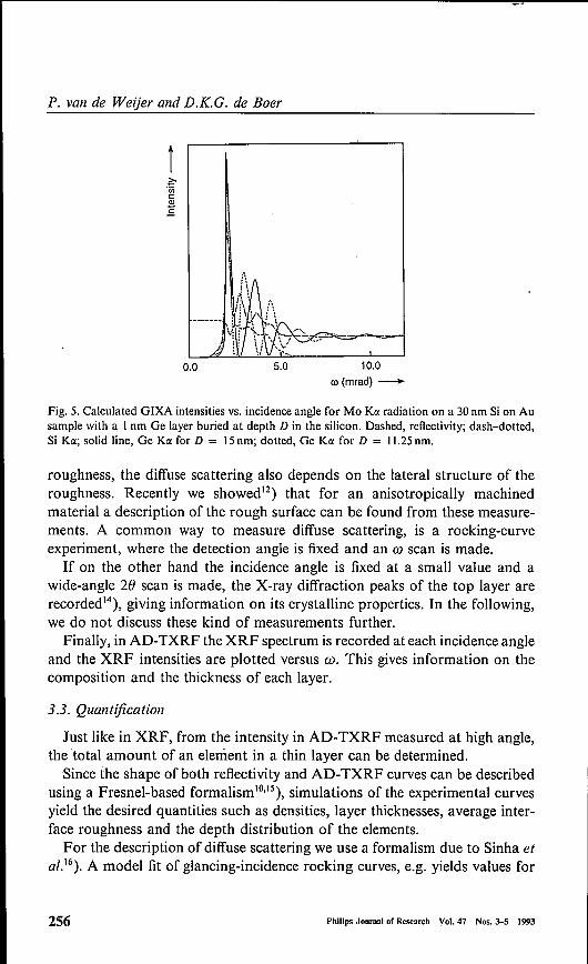
Fig. 5. Calculated GIXA intensities vs. incidence angle for Mo Ka radiation on a 30 nm Si on Ausample with a Inm Ge layer buried at depth D in the silicon. Dashed, reflectivity; dash-dotted,Si Ka; solid line, Ge Ka for D = 15nm; dotted, Ge Ka for D = 11.25nm.

roughness, the diffuse scattering also depends on the lateral structure of theroughness. Recently we showed") that for an anisotropically machinedmaterial a description of the rough surface can be found from these measure-ments. A common way to measure diffuse scattering, is a rocking-curveexperiment, where the detection angle is fixed and an (I) scan is made.

If on the other hand the incidence angle is fixed at a small value and awide-angle 2e scan is made, the X-ray diffraction peaks of the top layer arerecorded"), giving information on its crystalline properties. In the following,we do not discuss these kind of measurements further.

Finally, in AD-TXRF the XRF spectrum is recorded at each incidence angleand the XRF intensities are plotted versus (I). This gives information on thecomposition and the thickness of each layer.

3.3. Quantification

Just like in XRF, from the intensity in AD-TXRF measured at high angle,the total amount of an element in a thin layer can be determined.

Since the shape ofboth reflectivity and AD-TXRF curves can be describedusing a Fresnel-based forrnalism'S"), simulations of the experimental curvesyield the desired quantities such as densities, layer thicknesses, average inter-face roughness and the depth distribution of the elements.

For the description of diffuse scattering we use a formalism due to Sinha etal.16). A model fit of glancing-incidence rocking curves, e.g. yields values for

256 Philips Journal of Research Vol.47 Nos. 3-5 1993

Philips Journalof Research Vol. 47 Nos.3-5 1993 257


z-'inc:Q)

.5 1.0

0.0 L...o..::L.....J...__--'--_--'-_---'- _ __'0.0 2.0 4.0 6.0 8.0 10.0

m(mrad)-

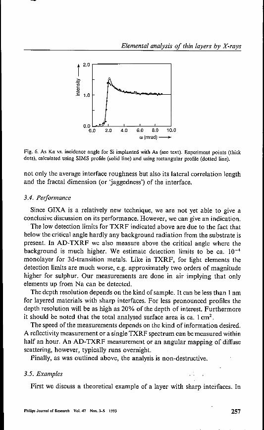
Fig. 6. As Ka vs. incidence angle for Si implanted with As (see text). Experiment points (thickdots), calculated using SIMS profile (solid line) and using rectangular profile (dotted line).

not only the average interface roughness but also its lateral correlation lengthand the fractal dimension (or 'jaggedness') of the interface.

3.4. Performance

Since GIXA is a relatively new technique, we are not yet able to give aconclusive discussion on its performance. However, we can give an indication.The low detection limits for TXRF indicated above are due to the fact that

below the critical angle hardly any background radiation from the substrate ispresent. In AD-TXRF we also measure above the critical angle where thebackground is much higher. We estimate detection limits to be ca. 10-4monolayer for 3d-transition metals. Like in TXRF, for light elements thedetection limits are much worse, e.g. approximately two orders of magnitudehigher for sulphur. Our measurements are done in air implying that onlyelements up from Na can be detected.The depth resolution depends on the kind of sample. It can be less than 1nm

for layered materials with sharp interfaces. For less pronounced profiles thedepth resolution will be as high as 20% of the depth of interest. Furthermoreit should be noted that the total analysed surface area is ca. 1cm",The speed of the measurements depends on the kind of information desired.

A reflectivitymeasurement or a single TXRF spectrum can bemeasured withinhalf an hour. An AD- TXRF measurement or an angular mapping of diffusescattering, however, typically runs overnight.Finally, as was outlined above, the analysis is non-destructive.

3.5. Examples

First we discuss a theoretical example of a layer with sharp interfaces. In


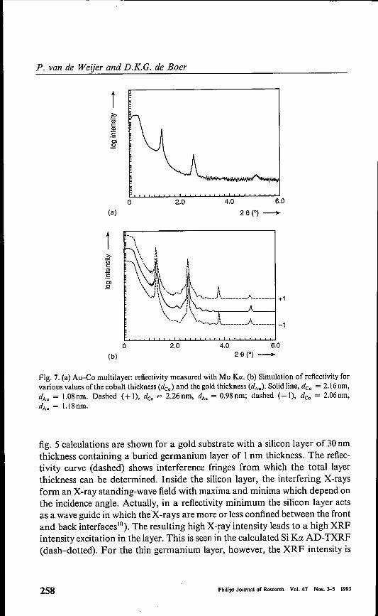
Fig. 7. (a) Au-Co multilayer: reflectivity measured with Mo Koe.(b) Simulation of reflectivity forvarious values of the cobalt thickness (deo) and the gold thickness (dA.). Solid line, deo = 2.16 nm,dAU = 1.08 nm. Dashed (+ I), deo = 2.26 nm, dAu = 0.98 nm; dashed (- I), deo = 2.06 om,dAu = 1.18 om.

fig. 5 calculations are shown for a gold substrate with a silicon layer of 30nmthickness containing a buried germanium layer of 1nm thickness. The reflec-tivity curve (dashed) shows interference fringes from which the total layerthickness can be determined. Inside the silicon layer, the interfering X-raysform an X-ray standing-wave field with maxima and minima which depend onthe incidence angle. Actually, in a reflectivity minimum the silicon layer actsas a wave guide in which the X-rays are more or less confined between the frontand back interfaces"). The resulting high X-ray intensity leads to a high XRFintensity excitation in the layer. This is seen in the calculated Si KO(AD-TXRF(dash-dotted). For the thin germanium layer, however, the XRF intensity is

258

Î.~(J)c~.s

0(a)

Î.?;-·incOl

.SCl..Q

2.0 4.0 6.0

28(°) -

o 2.0 4.0 6.028(°) -(b)

Philips Journal of Research Vol.47 Nos. 3-5 1993


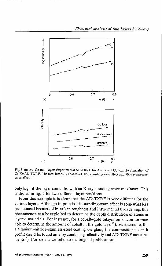
Fig. 8. (a) Au-Co multilayer: Experimental AD-TXRF for Au La and Co Ka. (b) Simulation ofCo Ka·AD-TXRF. The total intensity consists of30% standing-wave effect and 70% evanescent-wave effect.

only high if the layer coincides with an X-ray standing-wave maximum. Thisis shown in fig. 5 for two different layer positions.From this example it is clear that the AD- TXRF is very different for the

various layers. Although in practice the standing-wave effect is somewhat lesspronounced because of interface roughness and instrumental broadening, thisphenomenon can be exploited to determine the depth distribution of atoms inlayered materials. For instance, for a cobalt-gold bilayer on silicon we wereable to determine the amount of cobalt in the gold layer"). Furthermore, fora titanium-nitride-stainless-steel coating on glass, the compositional depthprofile could be found only by combining reflectivity and AD-TXRF measure-ments"). For details we refer to the original publications. .

iz-'iiicID

£<J)

.Q

0(al

Îz-'iiicID.s

0.6 0.7 0.8

Ol (Ol --+-

Co total

-----------------------------------------------<ordered..-_ ..- ......_------------------_.---_ ......-----_ ..--_ ....-

0.6 0.7 0.8Ol (Ol --+-(bl

Philips Journal of Research VoI.47 Nos. 3-5 1993 259


iz- 20000ëiicOl.s

0.5 1.0

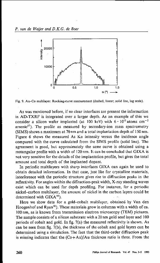
Fig. 9. Au-Co multilayer: Rocking-curve measurement (dashed, linear; solid line, log scale).

As was mentioned before, if no clear interfaces are present the informationin AD-TXRF is integrated over a larger depth. As an example of this weconsider a silicon wafer implanted (at 100 keY) with 6· 1015 atoms cm"?arsenic"). The profile as measured by secondary-ion mass speetrometry(SIMS) shows a maximum at 70nm and a total implantation depth of 150nm.Figure 6 shows the measured As K« intensity versus the incidence anglecompared with the curve calculated from the SIMS profile (solid line). Theagreement is good, but approximately the same curve is obtained using arectangular profile with a width of 120nm. It can be concluded that GIXA isnot very sensitive for the details of the implantation profile, but gives the totalamount and total depth of the implanted dopant.In periodic multilayers with sharp interfaces GIXA can again be used to

obtain detailed information. In that case, just like for crystalline materials,interference with the periodic structure gives rise to diffraction peaks in thereflectivity. For angles within the diffraction-peak width, X-ray standing wavesexist which can be used for depth profiling. For instance, for a periodicnickel-carbon multilayer, the amount of nickel in the carbon layers could bedetermined with GIXAIO

).

Here we show data for a gold-cobalt multilayer, obtained by Van denHoogenhof and Ryan 18). These materials grow in columns with a width of ca.100nm, as is known from transmission electron microscopy (TEM) pictures.The sample consists of a silicon substrate with a 20nm gold seed layer and 100periods of cobalt and gold. In fig. 7(a) the measured reflectivity is shown. Ascan be seen from fig. 7(b), the thickness of the cobalt and gold layers can bedetermined using a simulation. The fact that the third-order diffraction peakis missing indicates that the (Co-j-Auj/Au thickness ratio is three. From the

260 Philips Journalof Research Vol.47 Nos. 3-5 1993

Philips Journal of Research Vol.47 Nos. 3-5 1993 261


simulation it was also found that the interface roughness changes graduallyfrom 0.35 nm at the substrate to I nm at the top"). Figure 8(a) shows theAD-TXRF measurements for this sample. A modulation of the intensities isseen, but it is approximately a factor of th ree less pronounced than is expectedfor an ideal multilayer. The reason for this is that part of the sample is notordered enough for standing-wave formation. A simulation (fig. 8(b)) showsthat the ordered (or coherent) fraction is ca. 30%. Probably the non-orderedpart is at the column borders. Figure 9 shows the rocking curve with thedetector at the 28 of the first-order diffraction peak. Besides a sharp specularpeak, diffuse scattering tails are seen with a width of ca. 1°. This correspondsto a lateral roughness correlation of ca. lOOnm, which is in agreement with theexpected order of magnitude for the column distance. There seems to be acontradiction with the interface bending at the column borders of severaldegrees infered from TEM and X-ray diffraction"). From this one mightexpect a rocking curve with a width ofseveral degrees instead of 1°. We believethat at the column borders the X-rays are not backscattered but transmittedand absorbed, as can be seen from the AD-TXRF data. For this rathercomplicated example it can be concluded that GrXA helps to obtain a pictureof the sample, not only of the depth profile, but also of the lateral structure.

4. Conclusions

XRF based on the fundamental parameter approach is a fast and precisetechnique for measuring the elemental composition and the thickness ofthin-layer samples. As the accuracy of an application is not known in advanceowing to uncertainties in the fundamental parameter calibration procedure, areference analysis is necessary to determine this accuracy. Therefore, webelieve that XRF is especially appropriate for elemental analysis when theapplication concerns a large number of similar samples.

GrXA is an emerging technique for non-destructive depth analysis, which bycombining AD-TXRF, reflectivity and rocking curves, can yield detailedinformation on the distribution of elements in more complex layered samples.

REFERENCES

I) E.P. Bertin, Principles and Practice ofX-ray Spectrometric Analysis, Plenum Press, New York,1975.

2) R. Tertian and F. Claisse, Principles of Quantitative X-ray Fluorescence Analysis, Heyden,London, 1982.

3) Application Study 91003, Philips Analytical, Almelo, 1991.4) D.K.G. de Boer and P.N. Brouwer, Adv. X-ray Anal. 33, 237 (1990).5) D.K.G. de Boer, X-ray Spectrom., 19, 145 (1990)..6) D.K.G. de Boer, l.J.M. Borstrok, A.l.G. Leenaers, H.A. van Sprang and P.N. Brouwer, X-ray

Spectrom., 22, 33 (1993).


7) N. Parekh, C. Nieuwenhuizen, J. Borstrok and O. Elgersma, J. Electrochem. Soc., 138, 1460(1991).

8) D.K.G. de Boer, X-ray Spectrom., 18 119 (1989).9) A. Prange and H. Schwenke, Adv. X-ray Anal., 35 (1992).10) D.K.G. de Boer, Phys. Rev. B, 44, 498 (1991).") U. Weisbrod, R. Gutschke, J. Knoth and H. Schwenke, Appl. Phys. A, 53,449 (1991).12) W.W. van den Hoogenhof and D.K.G. de Boer, Spectrochim. Acta, 48B, 277 (1993).13) C. Schiller, G.M. Martin, W. van den Hoogenhofand J. Corno, Philips J. Research, this issue.14) T.C. Huang, Adv. X-ray Anal., 33, 91 (1990).IS) L.G. Parratt, Phys. Rev., 95, 359 (1954).16) S.K. Sinha, E.B. Sirota, S. Garoff and H.B. Stanley, Phys. Rev. B, 38, 2297 (1988).17) D.K.G. de Boer and W.W. van den Hoogenhof, Adv. X-ray Anal., 34, 35 (1991).18) W.W. van den Hoogenhof and T.W. Ryan, J. Magn. Magn. Mater., in press.

AuthorsPeter van de Weijer studied chemistry at the State University of Utrecht (1968-1974). In his thesis,at the Twente University of Technology (1977),he described acid-base properties ofaza-aromatics,as investigated by nuclear magnetic resonance. At the Philips Research Laboratories (1977- ), hestarted with mechanistic studies on low-pressure mercury discharges by laser-diagnostic measure-ments. With the.same technique he investigated the mechanisms oflow-pressure chemical vapourdeposition and the operation of a nitrogen-phosphorus detector as used in chromatography. Inthe Analytical Chemistry Department he was involved in inductively coupled plasma massspeetrometry and, subsequently, in X-ray fluorescence.

Dick de Boer studied physical chemistry at the State University of Groningen, where he obtainedhis PhD in 1983 on Electronic Structure Determination by Photoelectron Spectroscopy. Then heworked two years in surface analysis at Océ Van der Grinten, Venlo, The Netherlands. At PhilipsResearch Laboratories Eindhoven (1985- ) he did research in X-ray analysis. A main part of hiswork was the development of a fundamental-parameter method for XRF analysis of layeredmaterials. Subsequently he started to exploit the possibilities of glancing-incidence X-ray analysisand to develop theory and instrumentation for it.

262 Philips Journalof Research Vol.47 Nos. 3-5 1993

elemental analysis of thin layers byx-rays bound... · elemental analysis of thin layers by x-rays...

Documents