Transportation Research Part F 13 (2010) 71–79

Contents lists available at ScienceDirect

Transportation Research Part F

journal homepage: www.elsevier .com/locate / t r f

Electronic records of undesirable driving events

Oren Musicant *, Hillel Bar-Gera, Edna SchechtmanDepartment of Industrial Engineering and Management, Ben-Gurion University of the Negev, P.O.B. 65, 84105 Beer-Sheva, Israel

a r t i c l e i n f o

Article history:Received 28 April 2008Received in revised form 27 October 2009Accepted 2 November 2009

Keywords:Driver behaviorNegative-Binomial distributionIn-vehicle data recorders

1369-8478/$ - see front matter � 2009 Elsevier Ltddoi:10.1016/j.trf.2009.11.001

* Corresponding author. Tel.: +972 52 4524422; fE-mail address: misucant@bgu.ac.il (O. Musicant

a b s t r a c t

The cause of the majority of road crashes can be attributed to drivers’ behavior. Recent in-vehicle monitoring technologies enable continuous and high resolution measurements ofdrivers’ behaviors. We analyzed the information received from a novel in-vehicle technol-ogy which identifies the occurrences of undesirable driving events such as extreme brakingand accelerating, sharp cornering and sudden lane changing. We undertook an exploratoryanalysis to provide better understanding of events frequency (EF) statistical properties. Ourfindings show higher EF in trip edges (trip beginning and trip end) than in the middle of thetrip, higher EF for males than for females and higher EF at nighttime than at daytime. Use ofthe in-vehicle technology’s continuous and high resolution measurements enabled inter-esting advanced statistical analyses. Future research can use our findings to build similarstatistical models to predict the occurrence of undesirable driving events by other indepen-dent variables.

� 2009 Elsevier Ltd. All rights reserved.

1. Introduction

The cause for the overwhelming majority of road crashes can be attributed to driver’s unsafe behavior (Evans, 2004, p.337). Understanding driver’s unsafe behavior is therefore valuable in order to improve road safety. Research is in a contin-uance search for new variables to better describe driver’s behavior, for new methods to measure those variables and for newmethods to analyze the measured information. This study discusses a surrogate for safety, the frequency of certain drivingevents such as extreme braking, sudden lane changes and improper turning.

Indeed in principle extreme maneuvers may be performed by skilled drivers as a safe response to unexpected conditions,but more often than not situations where extreme maneuvers are needed can be avoided by a safe driving style. Therefore,from a statistical point of view high frequency of events is an indication of unsafe driving, and the events themselves can beconsidered as ‘‘undesirable.”

Undesirable events frequency (EF) is a useful safety surrogate as such events were found to be related to crash involve-ment and driver safety. For example, in the US about 9% of all police-reported crashes in 1996 were related to lane changing(Sen, Smith, & Najm, 2003). McGwin and Brown (1999) analyzed over 100,000 crash records and reported that in nearly 50%of the cases some sort of driving event (turning, lane changing and reversing) preceded the crash and in about 6% of thecases, it was the primary cause of the crash. Another study by Jun, Ogle, and Guensler (2007) examined differences incrash-involved drivers versus non-involved drivers and found that extreme braking events occur more frequently tocrash-involved drivers in certain travel times and road types. Those differences were more pronounced on freeways inthe morning hours, where non-involved drivers had 0.009 braking events per mile and crash-involved drivers had 0.029braking events per mile (difference is 71%). Extreme braking was also associated with inattentiveness (see Hancock, Lesch,& Simmons, 2003; Jamson & Merat, 2005) and driving under the influence of alcohol, as drunk drivers exhibited a more

. All rights reserved.

ax: +972 9 7494584.).

72 O. Musicant et al. / Transportation Research Part F 13 (2010) 71–79

aggressive driving style, following closer to the vehicle in front of them and applying more force while braking (Strayer,Drews, & Crouch, 2003).

In normal driving situations drivers are required to turn, change lanes and apply force when using the braking pedal. Suchdriving events are considered undesired when their performance contributes to a decrease in driver safety. Thus, surrogatesfor safety variables such as speed, acceleration time and distance are often used to distinguish between driving events indifferent situations: Liu and Lee (2005) used time to stop and deceleration in braking events to compare drivers’ perfor-mances while in real driving approaching red light (12 drivers and 24 intersections). Drivers using a car phone demonstratedlower approach speed, but also lower time to stop and more intense deceleration. The researchers also used questionnairesto classify drivers to aggressive and non-aggressive. They found that aggressive drivers approach intersections in higherspeed and compensate by more instant deceleration (p. 376). McGehee, Raby, Carney, Lee, and Reyes (2007) used video re-cords of young drivers’ driving events. Rather than supplying enormous amount of video data the recorder was triggeredwhen the acceleration of the vehicle exceeded a set threshold in the lateral (hard cornering) or longitude (sharp braking)direction. They found that parental intervention is useful in reducing the frequency of the events in teens driving.

The means of recording safety surrogate physical variables have recently further improved with the introduction of in-vehicle data recorders (IVDRs). IVDR technology enables the measurement of common safety surrogates as velocity, accel-eration and vehicle position. Several studies indicate the potential of the use of IVDRs to measure driver behavior: Boyce andGeller (2001) used a ‘‘smart car” instrumented with video cameras and sensors for acceleration to record driver behaviors inreal driving situations (N = 61). Human observers coded the raw data into discrete events of close following, unsafe speed,proper use of turn signaling, maintaining lane position, and engaging in secondary tasks (as adjusting the radio button). Theresearchers graphically analyzed the proportion of safe events versus driver age and discovered that for younger drivers thisproportion was lower (no significance tests were reported). They emphasized the potential in sensor technology to measuremultiple driver behaviors without the possible bias in driver self reports.

In an ambitious naturalistic driving study 100 vehicles were instrumented with multiple sensors of GPS, accelerometers,video cameras, radar sensors and lane trackers (Neale et al., 2002). The data collected over a 13 months period consists ofover 43,000 h and 2 million miles driven. This information was attached to a database of crashes, near-crashes, and otherincidents (crash-relevant conflicts and proximity conflicts) to describe each of these occurrences by parameters as pre-crashmaneuver, avoidance maneuver, speed, time-to-collision, and driver reaction time (Neale, Dingus, Klauer, Sudweeks, &Goodman, 2005). The analysis of this large amount of information includes a variety of safety related topics such as drivers’inattentiveness, classification of crashes by drivers’ performance data, analysis of rear-end and lane changing crashes andmany more (Dingus et al., 2006). These studies indicate that detailed and objective information provided by IVDRs is usefulfor learning about many driver behaviors enhancing human knowledge and potentially even save lives.

The vast raw information of speed, acceleration and video recordings provided by the IVDRs may be too detailed, andtherefore should be reduced to identify patterns of interest. Such patterns of interest can be the undesirable driving eventsthat are in the focus of this study. The automated identification of undesirable driving events is not a trivial task, because itrequires some automated interpretation of the raw data. In this paper we use a specialized IVDR named the Green-Box whichis able to automatically detect and report the occurrence of undesirable driving events.

The rest of the paper is organized as follows: In Section 2 we provided a detailed description of the Green-Box measure-ment and system framework. The following section describes the objectives of the study and the analytical methods used inthe exploratory analysis of the information received from the IVDR. Sections 4 and 5 describe the results of the study dis-cussing the process of fitting a distribution to the events frequency (EF) and building several regression models with drivingtime and driver gender as explanatory variables for EF. Section 6 summarizes our main findings and discusses possibleimplementations.

2. The Green-Box

The Green-Box is an in-vehicle data recorder (IVDR) designed to provide drivers with feedback on their driving behavior.The Green-Box reports commonly used measures of speed, travel time, distance and location. Yet, its novelty lies in the real-time identification of undesirable driving events such as extreme breaking and accelerating, sharp turning and sudden lanechanging. Several studies found a correlation between the frequency of events identified by this device and crash involve-ment records (Musicant, Lotan, & Toledo, 2007; Toledo & Lotan, 2006; Toledo, Musicant, & Lotan, 2008).

The Green-Box contains sensors for speed (GPS) and acceleration (accelerometers) that feed the raw data into a specialprocessing unit which is able to identify the occurrence of driving events. The amount of data collected by the various sen-sors is very large. Speed and location are recoded every second and the acceleration of the vehicle is sampled 40 times persecond in both lateral and longitudinal directions. Pattern recognition algorithms are applied to the raw data in order to de-tect over 20 different basic maneuver categories such as lane changes and turns with and without acceleration, suddenbrakes, extreme accelerations, and so on. The information is transmitted in real time via cellular network to an applicationserver where this information is further analyzed to create several driver indices and statistics that can be used to charac-terize driver behavior.

This information is used by commercial fleets and insurance companies to encourage safer driving and enable drivers(and their supervisors) to moderate their driving via the feedback they are receiving. The side benefit for studies as this

O. Musicant et al. / Transportation Research Part F 13 (2010) 71–79 73

one is the availability of extremely large data sets containing information on driver behavior in real driving conditions (seefor example Lotan, Toledo, & Prato, 2009; Prato, Lotan, & Toledo, 2009).

3. Objective and analytical methods

The Green-Box information is based on raw measurements of speed and acceleration. This information was found to berelated to driver safety. Yet research effort in investigating this novel information is just beginning. The purpose of this studyis to gain a deeper understanding about the frequency of events mainly with regard to trip characteristics such as the tripduration, the time of the day, and the day of the week. In addition we also considered driver gender. We analyzed the eventsfrequency (EF) in 117,195 trips with duration of 2–90 min. The information was collected over a 6 months period for 109drivers (23 females). Details provided for each trip entry are: trip date and time, trip duration, and the number of events.Each vehicle has a main driver, whose gender is known. In the lack of a better alternative, we assumed that all trips of a vehi-cle are performed by its main driver.

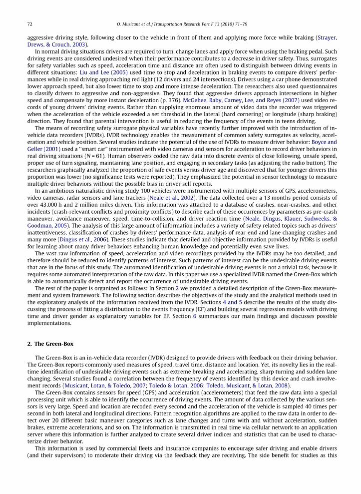
First, we used the Maximum likelihood estimation method in order to fit a distribution to EF. Because our variable ofinterest is a count variable, the most basic Poisson distribution was initially considered. Assuming a Poisson distribution im-plies that the mean and the variance should be equal. Yet, we found that for each given trip duration the variance was largerthan the average count of events (Fig. 1). Thus, we chose the Negative-Binomial distribution which is a generalization of thePoisson distribution that does allow mean and variance to be different.

The fit of the Negative-Binomial distribution was evaluated by the v2 goodness of fit test and various graphical methods.We also implemented several Negative-Binomial regression models with driving time, driver gender and the interaction be-tween them as explanatory variables for EF.

4. Events count and events frequency

Our variable of interest is the event frequency (EF) given by the count of events per minute of driving, thus a choice ofPoisson or Negative-Binomial as the underlying distribution seemed appropriate. While the random variable in the basicPoisson model is the count of events, in most cases it is more convenient to look at the estimated parameter lambda thatrepresents the frequency of events per minute. This required an assumption that EF is constant for any given trip duration.

Fig. 1. Mean and variance of event count per trip duration. *EF variance is given in square units.

0.00

0.02

0.04

0.06

0.08

0.10

0.12

0 10 20 30 40 50 60 70 80 90Trip Duration (Minutes)

EF

Fig. 2. Average number of events per minute (dots) and confidence intervals (a = 0.05) by trip duration.

10 minutes trips

0.00

0.02

0.040.06

0.08

0.10

1 2 3 4 5 6 7 8 9 10Time from trip beginning (minutes)

EF

15 minutes trips

0.000.020.04

0.060.080.10

1 2 3 4 5 6 7 8 9 10 11 12 1314 15Time from trip beginning (minutes)

EF

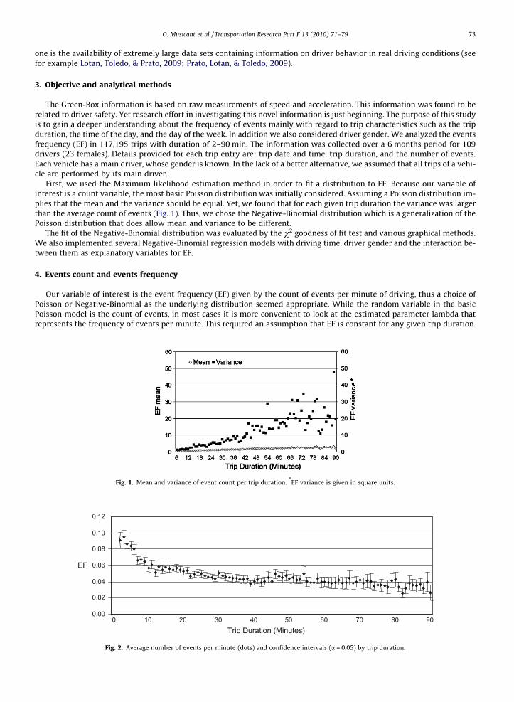
Fig. 3. Average number of events at each minute from trip beginning.

0.04

0.05

0.06

0.07

0.08

0.09

0.10

1 2 3 4 5Minutes from trip begining

EF

0.04

0.05

0.06

0.07

0.08

0.09

0.10

12345Minutes from trip ending

EF

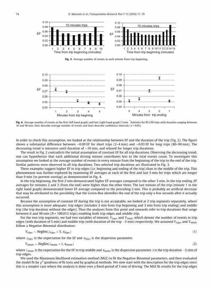
Fig. 4. Average number of events at the first (left hand graph) and last (right hand graph) 5 min. *Statistics for 85,190 trips with duration ranging between10 and 90 min. Dots describe average number of events and lines describe confidence intervals (a = 0.05).

74 O. Musicant et al. / Transportation Research Part F 13 (2010) 71–79

In order to check this assumption, we looked at the relationship between EF and the duration of the trip (Fig. 2). The figureshows a substantial difference between �0.09 EF for short trips (2–4 min) and �0.03 EF for long trips (80–90 min). Thedecreasing trend is intensive until duration of �10 min, and relaxed for longer trip durations.

The result in Fig. 2 contradicts the initial assumption of constant EF for all trip durations. Observing the decreasing trend,one can hypothesize that each additional driving minute contributes less to the total events count. To investigate thisassumption we looked at the average number of events in every minute from the beginning of the trip to the end of the trip.Similar patterns were observed in all trip durations. Two selected trip durations are illustrated in Fig. 3.

These examples suggest higher EF in trip edges (i.e. beginning and ending of the trip) than in the middle of the trip. Thisphenomenon was further explored by examining EF averages at each of the first and last 5 min for trips which are longerthan 9 min (to prevent overlap) as demonstrated in Fig. 4.

In the trip beginning, the first 2 min demonstrated higher EF averages compared to the other 3 min. In the trip ending, EFaverages for minutes 2 and 3 (from the end) were higher than the other three. The last minute of the trip (minute 1 in theright hand graph) demonstrated lower EF average compared to the preceding 2 min. This is probably an artificial decreasethat may be attributed to the possibility that the Green-Box identifies the end of the trip only a few seconds after it actuallyoccurred.

Because the assumption of constant EF during the trip is not acceptable, we looked at 2 trip segments separately, wherethis assumption is more adequate: trip edges (includes 2 min from trip beginning and 3 min from trip ending) and middletrip (the trip duration without the edges). Thus the analyses from this point and onwards refer to trip durations that rangebetween 6 and 90 min (N = 100,013 trips) enabling both trip edges and middle trip.

For the two trip segments, we had two variables of interest; YEdges and YMiddle which denote the number of events in tripedges (with duration of 5 min) and middle trip (with duration of the trip �5 min) respectively. We assumed YEdges and YMiddle

follow a Negative-Binomial distribution:

YEdges � NegbinðkEdges � 5;aEdgesÞ ð1Þ

where kEdges is the expectation for the EF and aEdges is the dispersion parameter.

YMiddle � NegbinðkMiddle � t;aMiddleÞ ð2Þ

where kMiddle is the expectation for the EF in trip middle and aMiddle is the dispersion parameter. t is the trip duration�5 min oftrip edges.

We used the Maximum likelihood estimation method (MLE) to fit the Negative-Binomial parameters, and then evaluatedthe model fit by v2 goodness of fit tests and by graphical methods. We now start with the description for the trip edges sincethis is a simpler case where the analysis is done over a fixed period of 5 min of driving. The MLE fit results for the trip edges

12.862.822.82

4.260.10

0.241.441.83

0.725.24

21.4317.59

23.14

0.05

1

10

100

1000

10000

100000

0 1 2 3 4 5 6 7 8 9 10 11 12 13-19

Event count

Freq

uenc

y

Observed Expected

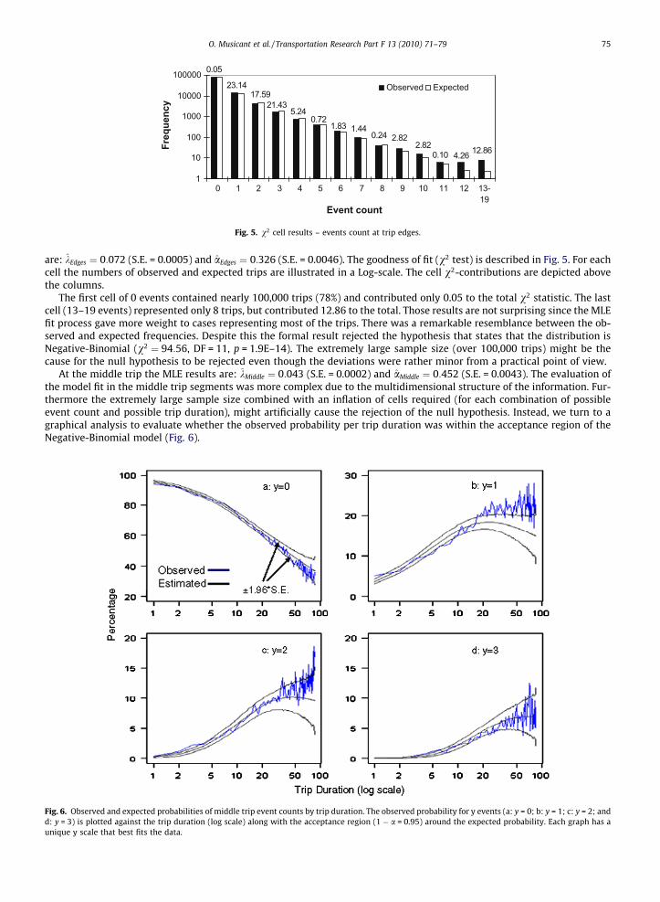
Fig. 5. v2 cell results – events count at trip edges.

O. Musicant et al. / Transportation Research Part F 13 (2010) 71–79 75

are: kEdges ¼ 0:072 (S.E. = 0.0005) and aEdges ¼ 0:326 (S.E. = 0.0046). The goodness of fit (v2 test) is described in Fig. 5. For eachcell the numbers of observed and expected trips are illustrated in a Log-scale. The cell v2-contributions are depicted abovethe columns.

The first cell of 0 events contained nearly 100,000 trips (78%) and contributed only 0.05 to the total v2 statistic. The lastcell (13–19 events) represented only 8 trips, but contributed 12.86 to the total. Those results are not surprising since the MLEfit process gave more weight to cases representing most of the trips. There was a remarkable resemblance between the ob-served and expected frequencies. Despite this the formal result rejected the hypothesis that states that the distribution isNegative-Binomial (v2 ¼ 94:56, DF = 11, p = 1.9E–14). The extremely large sample size (over 100,000 trips) might be thecause for the null hypothesis to be rejected even though the deviations were rather minor from a practical point of view.

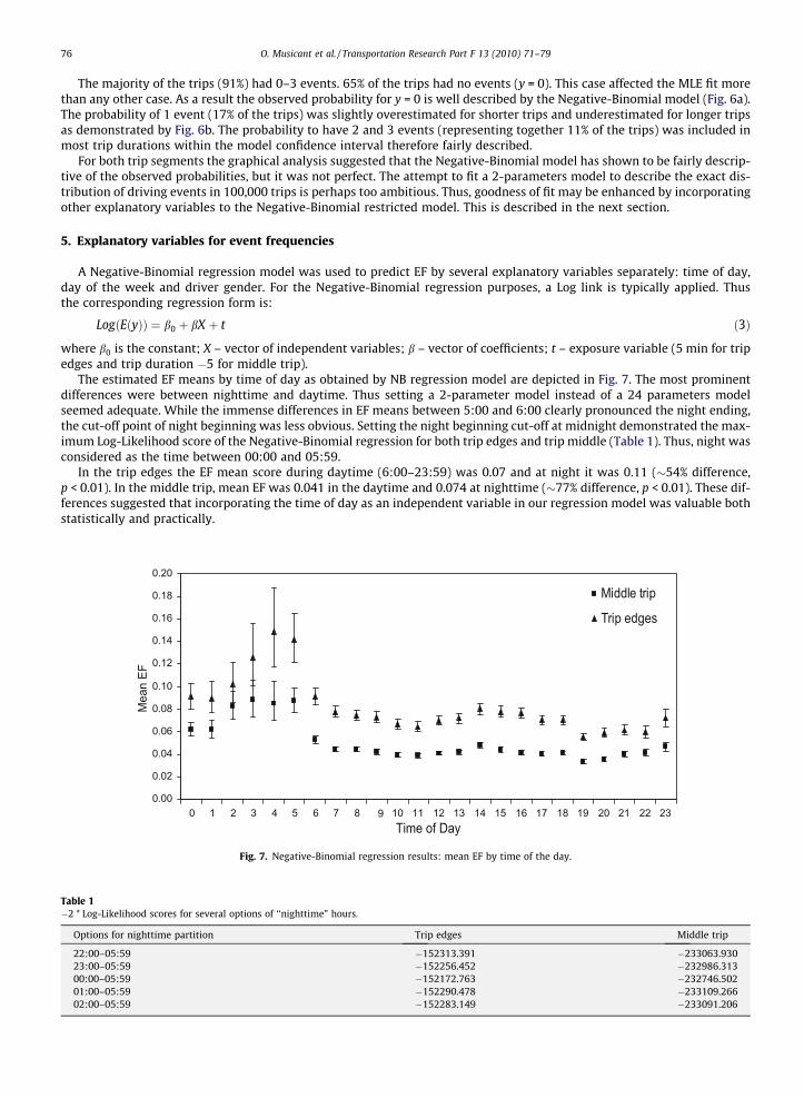
At the middle trip the MLE results are: kMiddle ¼ 0:043 (S.E. = 0.0002) and aMiddle ¼ 0:452 (S.E. = 0.0043). The evaluation ofthe model fit in the middle trip segments was more complex due to the multidimensional structure of the information. Fur-thermore the extremely large sample size combined with an inflation of cells required (for each combination of possibleevent count and possible trip duration), might artificially cause the rejection of the null hypothesis. Instead, we turn to agraphical analysis to evaluate whether the observed probability per trip duration was within the acceptance region of theNegative-Binomial model (Fig. 6).

Fig. 6. Observed and expected probabilities of middle trip event counts by trip duration. The observed probability for y events (a: y = 0; b: y = 1; c: y = 2; andd: y = 3) is plotted against the trip duration (log scale) along with the acceptance region (1 � a = 0.95) around the expected probability. Each graph has aunique y scale that best fits the data.

76 O. Musicant et al. / Transportation Research Part F 13 (2010) 71–79

The majority of the trips (91%) had 0–3 events. 65% of the trips had no events (y = 0). This case affected the MLE fit morethan any other case. As a result the observed probability for y = 0 is well described by the Negative-Binomial model (Fig. 6a).The probability of 1 event (17% of the trips) was slightly overestimated for shorter trips and underestimated for longer tripsas demonstrated by Fig. 6b. The probability to have 2 and 3 events (representing together 11% of the trips) was included inmost trip durations within the model confidence interval therefore fairly described.

For both trip segments the graphical analysis suggested that the Negative-Binomial model has shown to be fairly descrip-tive of the observed probabilities, but it was not perfect. The attempt to fit a 2-parameters model to describe the exact dis-tribution of driving events in 100,000 trips is perhaps too ambitious. Thus, goodness of fit may be enhanced by incorporatingother explanatory variables to the Negative-Binomial restricted model. This is described in the next section.

5. Explanatory variables for event frequencies

A Negative-Binomial regression model was used to predict EF by several explanatory variables separately: time of day,day of the week and driver gender. For the Negative-Binomial regression purposes, a Log link is typically applied. Thusthe corresponding regression form is:

Table 1�2 * Lo

Opti

22:023:000:001:002:0

LogðEðyÞÞ ¼ b0 þ bX þ t ð3Þ

where b0 is the constant; X – vector of independent variables; b – vector of coefficients; t – exposure variable (5 min for tripedges and trip duration �5 for middle trip).

The estimated EF means by time of day as obtained by NB regression model are depicted in Fig. 7. The most prominentdifferences were between nighttime and daytime. Thus setting a 2-parameter model instead of a 24 parameters modelseemed adequate. While the immense differences in EF means between 5:00 and 6:00 clearly pronounced the night ending,the cut-off point of night beginning was less obvious. Setting the night beginning cut-off at midnight demonstrated the max-imum Log-Likelihood score of the Negative-Binomial regression for both trip edges and trip middle (Table 1). Thus, night wasconsidered as the time between 00:00 and 05:59.

In the trip edges the EF mean score during daytime (6:00–23:59) was 0.07 and at night it was 0.11 (�54% difference,p < 0.01). In the middle trip, mean EF was 0.041 in the daytime and 0.074 at nighttime (�77% difference, p < 0.01). These dif-ferences suggested that incorporating the time of day as an independent variable in our regression model was valuable bothstatistically and practically.

0.00

0.02

0.04

0.06

0.08

0.10

0.12

0.14

0.16

0.18

0.20

0 1 2 3 4 5 6 7 8 9 10 11 12 13 14 15 16 17 18 19 20 21 22 23Time of Day

Mea

n EF

Middle trip

Trip edges

Fig. 7. Negative-Binomial regression results: mean EF by time of the day.

g-Likelihood scores for several options of ‘‘nighttime” hours.

ons for nighttime partition Trip edges Middle trip

0–05:59 �152313.391 �233063.9300–05:59 �152256.452 �232986.3130–05:59 �152172.763 �232746.5020–05:59 �152290.478 �233109.2660–05:59 �152283.149 �233091.206

0.00

0.02

0.04

0.06

0.08

0.10

Sun Mon Tue Wed Thu Fri SatWeek day

EF

Middle trip Trip edges

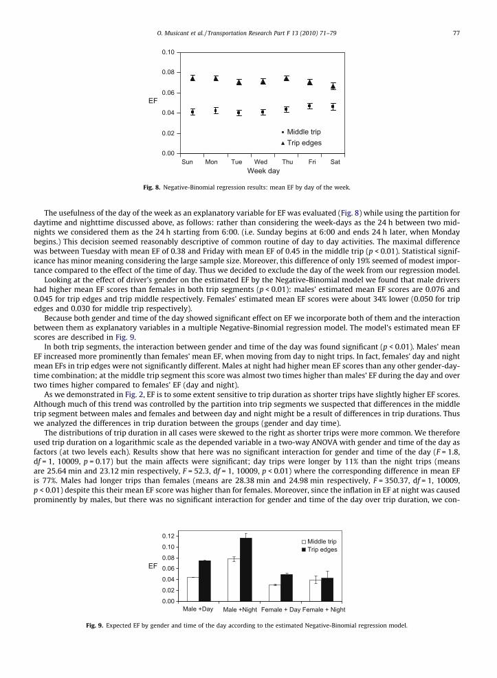
Fig. 8. Negative-Binomial regression results: mean EF by day of the week.

O. Musicant et al. / Transportation Research Part F 13 (2010) 71–79 77

The usefulness of the day of the week as an explanatory variable for EF was evaluated (Fig. 8) while using the partition fordaytime and nighttime discussed above, as follows: rather than considering the week-days as the 24 h between two mid-nights we considered them as the 24 h starting from 6:00. (i.e. Sunday begins at 6:00 and ends 24 h later, when Mondaybegins.) This decision seemed reasonably descriptive of common routine of day to day activities. The maximal differencewas between Tuesday with mean EF of 0.38 and Friday with mean EF of 0.45 in the middle trip (p < 0.01). Statistical signif-icance has minor meaning considering the large sample size. Moreover, this difference of only 19% seemed of modest impor-tance compared to the effect of the time of day. Thus we decided to exclude the day of the week from our regression model.

Looking at the effect of driver’s gender on the estimated EF by the Negative-Binomial model we found that male drivershad higher mean EF scores than females in both trip segments (p < 0.01): males’ estimated mean EF scores are 0.076 and0.045 for trip edges and trip middle respectively. Females’ estimated mean EF scores were about 34% lower (0.050 for tripedges and 0.030 for middle trip respectively).

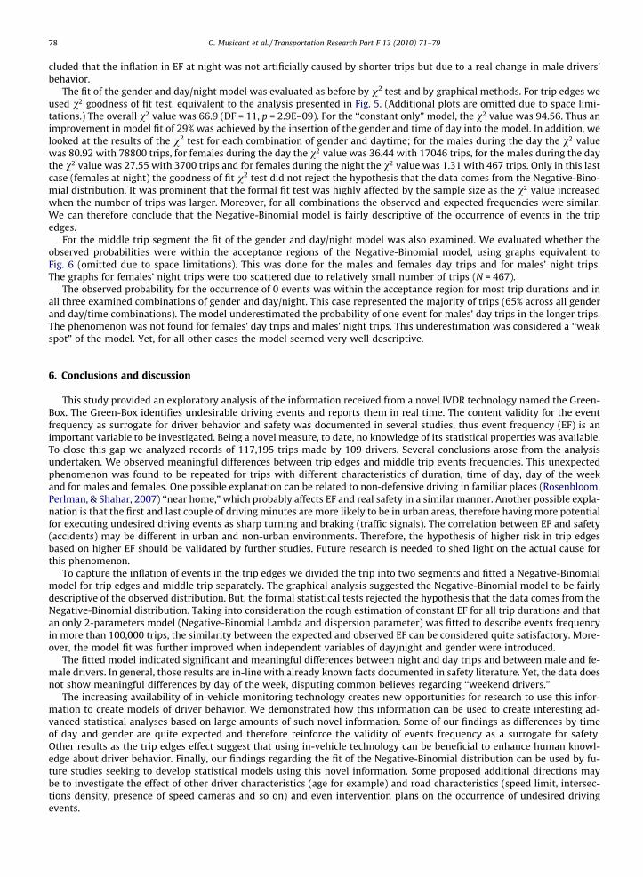
Because both gender and time of the day showed significant effect on EF we incorporate both of them and the interactionbetween them as explanatory variables in a multiple Negative-Binomial regression model. The model’s estimated mean EFscores are described in Fig. 9.

In both trip segments, the interaction between gender and time of the day was found significant (p < 0.01). Males’ meanEF increased more prominently than females’ mean EF, when moving from day to night trips. In fact, females’ day and nightmean EFs in trip edges were not significantly different. Males at night had higher mean EF scores than any other gender-day-time combination; at the middle trip segment this score was almost two times higher than males’ EF during the day and overtwo times higher compared to females’ EF (day and night).

As we demonstrated in Fig. 2, EF is to some extent sensitive to trip duration as shorter trips have slightly higher EF scores.Although much of this trend was controlled by the partition into trip segments we suspected that differences in the middletrip segment between males and females and between day and night might be a result of differences in trip durations. Thuswe analyzed the differences in trip duration between the groups (gender and day time).

The distributions of trip duration in all cases were skewed to the right as shorter trips were more common. We thereforeused trip duration on a logarithmic scale as the depended variable in a two-way ANOVA with gender and time of the day asfactors (at two levels each). Results show that here was no significant interaction for gender and time of the day (F = 1.8,df = 1, 10009, p = 0.17) but the main affects were significant; day trips were longer by 11% than the night trips (meansare 25.64 min and 23.12 min respectively, F = 52.3, df = 1, 10009, p < 0.01) where the corresponding difference in mean EFis 77%. Males had longer trips than females (means are 28.38 min and 24.98 min respectively, F = 350.37, df = 1, 10009,p < 0.01) despite this their mean EF score was higher than for females. Moreover, since the inflation in EF at night was causedprominently by males, but there was no significant interaction for gender and time of the day over trip duration, we con-

0.00

0.02

0.04

0.060.08

0.10

0.12

Male +Day Male +Night Female + Day Female + Night

EF

Middle tripTrip edges

Fig. 9. Expected EF by gender and time of the day according to the estimated Negative-Binomial regression model.

78 O. Musicant et al. / Transportation Research Part F 13 (2010) 71–79

cluded that the inflation in EF at night was not artificially caused by shorter trips but due to a real change in male drivers’behavior.

The fit of the gender and day/night model was evaluated as before by v2 test and by graphical methods. For trip edges weused v2 goodness of fit test, equivalent to the analysis presented in Fig. 5. (Additional plots are omitted due to space limi-tations.) The overall v2 value was 66.9 (DF = 11, p = 2.9E–09). For the ‘‘constant only” model, the v2 value was 94.56. Thus animprovement in model fit of 29% was achieved by the insertion of the gender and time of day into the model. In addition, welooked at the results of the v2 test for each combination of gender and daytime; for the males during the day the v2 valuewas 80.92 with 78800 trips, for females during the day the v2 value was 36.44 with 17046 trips, for the males during the daythe v2 value was 27.55 with 3700 trips and for females during the night the v2 value was 1.31 with 467 trips. Only in this lastcase (females at night) the goodness of fit v2 test did not reject the hypothesis that the data comes from the Negative-Bino-mial distribution. It was prominent that the formal fit test was highly affected by the sample size as the v2 value increasedwhen the number of trips was larger. Moreover, for all combinations the observed and expected frequencies were similar.We can therefore conclude that the Negative-Binomial model is fairly descriptive of the occurrence of events in the tripedges.

For the middle trip segment the fit of the gender and day/night model was also examined. We evaluated whether theobserved probabilities were within the acceptance regions of the Negative-Binomial model, using graphs equivalent toFig. 6 (omitted due to space limitations). This was done for the males and females day trips and for males’ night trips.The graphs for females’ night trips were too scattered due to relatively small number of trips (N = 467).

The observed probability for the occurrence of 0 events was within the acceptance region for most trip durations and inall three examined combinations of gender and day/night. This case represented the majority of trips (65% across all genderand day/time combinations). The model underestimated the probability of one event for males’ day trips in the longer trips.The phenomenon was not found for females’ day trips and males’ night trips. This underestimation was considered a ‘‘weakspot” of the model. Yet, for all other cases the model seemed very well descriptive.

6. Conclusions and discussion

This study provided an exploratory analysis of the information received from a novel IVDR technology named the Green-Box. The Green-Box identifies undesirable driving events and reports them in real time. The content validity for the eventfrequency as surrogate for driver behavior and safety was documented in several studies, thus event frequency (EF) is animportant variable to be investigated. Being a novel measure, to date, no knowledge of its statistical properties was available.To close this gap we analyzed records of 117,195 trips made by 109 drivers. Several conclusions arose from the analysisundertaken. We observed meaningful differences between trip edges and middle trip events frequencies. This unexpectedphenomenon was found to be repeated for trips with different characteristics of duration, time of day, day of the weekand for males and females. One possible explanation can be related to non-defensive driving in familiar places (Rosenbloom,Perlman, & Shahar, 2007) ‘‘near home,” which probably affects EF and real safety in a similar manner. Another possible expla-nation is that the first and last couple of driving minutes are more likely to be in urban areas, therefore having more potentialfor executing undesired driving events as sharp turning and braking (traffic signals). The correlation between EF and safety(accidents) may be different in urban and non-urban environments. Therefore, the hypothesis of higher risk in trip edgesbased on higher EF should be validated by further studies. Future research is needed to shed light on the actual cause forthis phenomenon.

To capture the inflation of events in the trip edges we divided the trip into two segments and fitted a Negative-Binomialmodel for trip edges and middle trip separately. The graphical analysis suggested the Negative-Binomial model to be fairlydescriptive of the observed distribution. But, the formal statistical tests rejected the hypothesis that the data comes from theNegative-Binomial distribution. Taking into consideration the rough estimation of constant EF for all trip durations and thatan only 2-parameters model (Negative-Binomial Lambda and dispersion parameter) was fitted to describe events frequencyin more than 100,000 trips, the similarity between the expected and observed EF can be considered quite satisfactory. More-over, the model fit was further improved when independent variables of day/night and gender were introduced.

The fitted model indicated significant and meaningful differences between night and day trips and between male and fe-male drivers. In general, those results are in-line with already known facts documented in safety literature. Yet, the data doesnot show meaningful differences by day of the week, disputing common believes regarding ‘‘weekend drivers.”

The increasing availability of in-vehicle monitoring technology creates new opportunities for research to use this infor-mation to create models of driver behavior. We demonstrated how this information can be used to create interesting ad-vanced statistical analyses based on large amounts of such novel information. Some of our findings as differences by timeof day and gender are quite expected and therefore reinforce the validity of events frequency as a surrogate for safety.Other results as the trip edges effect suggest that using in-vehicle technology can be beneficial to enhance human knowl-edge about driver behavior. Finally, our findings regarding the fit of the Negative-Binomial distribution can be used by fu-ture studies seeking to develop statistical models using this novel information. Some proposed additional directions maybe to investigate the effect of other driver characteristics (age for example) and road characteristics (speed limit, intersec-tions density, presence of speed cameras and so on) and even intervention plans on the occurrence of undesired drivingevents.

O. Musicant et al. / Transportation Research Part F 13 (2010) 71–79 79

Acknowledgments

This study is funded by Ran-Naor foundation in Israel. The second and third authors were partially supported by the BGUPaul Ivanier Center for Robotics Research and Production Management. We would also like to thank GreenRoad technologiesfor the unlimited direct access to the information received from the IVDRs.

References

Boyce, E. T., & Geller, E. S. (2001). A technology to measure multiple driving behaviors without self-report or participant reactivity. Journal of AppliedBehavior Analysis, 34(1), 39–55.

Dingus, T. A., Klauer, S. G., Neale, V. L., Petersen, A., Lee, S. E., Sudweeks, J., et al. (2006). The 100-car naturalistic driving study phase II – Results of the 100-car field experiment. Report DOT-HS-810-593, Department of Transportation, Washington, DC.

Evans, L. (2004). Traffic safety, Science Serving Society.Hancock, P. A., Lesch, M., & Simmons, L. (2003). The distraction effects of phone use during a crucial driving maneuver. Accident Analysis and Prevention, 35,

501–514.Jamson, A. H., & Merat, N. (2005). Surrogate in-vehicle information systems and driver behavior: Effects of visual and cognitive load in simulated rural

driving. Transportation Research Part F, 8, 79–96.Jun, J., Ogle, J., & Guensler, R. (2007). Relationships between crash involvement and temporal-spatial driving behavior activity patterns using GPS

instrumented vehicle data. In TRB 2007 annual meeting CD-ROM.Liu, B., & Lee, Y. (2005). Effects of car-phone use and aggressive disposition during critical driving maneuvers. Transportation Research Part F, 8, 369–382.Lotan, T., Toledo, T., & Prato, C. G. (2009). Modeling the behavior of novice young drivers using data from in-vehicle data recorders. In Proceedings of the fifth

International driving symposium on human factors in driver assessment, training, and vehicle design (pp. 491–498). Montana.McGehee, D. V., Raby, M., Carney, C., Lee, J. D., & Reyes, M. L. (2007). Extending parental mentoring using an event-triggered video intervention in rural teen

drivers. Journal of Safety Research, 38, 215–227.McGwin, G., & Brown, D. B. (1999). Characteristics of traffic crashes among young, middle-aged, and older drivers. Accident Analysis and Prevention, 3,

181–198.Musicant, O., Lotan, T., & Toledo, T. (2007). Safety correlation and implications of an in-vehicle data recorder on driver behavior. In Preprints of the 86th

transportation research board annual meeting. Washington, DC.Neale, V. L., Klauer, S. G., Knipling, R. R., Dingus, T. A., Holbrook, G. T., & Petersen A. (2002). The 100 car naturalistic driving study phase I: Experimental

design. Report DOT-HS-808-536, Department of Transportation, Washington, DC.Neale, V. L., Dingus, T. A., Klauer, S. G., Sudweeks, J., Goodman, M. (2005). An overview of the 100 car naturalistic study and findings, Paper Number 05-0400,

National Highway Traffic Safety Administration.Prato, C. G., Lotan, T., & Toledo T. (2009). Intra-familial transmission of driving behavior: Evidence from in-vehicle data recorders. In Proceedings of the 88th

transportation research board annual meeting. Washington, DC.Rosenbloom, T., Perlman, A., & Shahar, A. (2007). Women drivers’ behavior in well-known versus less familiar locations. Journal of Safety Research, 38(3),

283–288.Sen, B., Smith, J. D., Najm, W. G. (2003). Analysis of lane change crashes. Report DOT HS 809 571, Department of Transportation, Washington, DC.Strayer, D. L., Drews, F. A., & Crouch, D. J. (2003). Fatal distraction? A comparison of the cell-phone drivers and the drunk driver. In Proceedings of the second

international driving symposium on human factors in driver assessment, training and vehicle design.Toledo, T., & Lotan, T. (2006). In-vehicle data recorder for evaluation of driving behavior and safety. Transportation Research Record, 1953, 112–119.Toledo, T., Musicant, O., & Lotan, T. (2008). In-vehicle data recorders for monitoring and feedback on drivers’ behavior. Transportation Research Part C, 16(3),

320–331.