electronic journal of diﬀerential equations, … journal of diﬀerential equations, vol....

Electronic Journal of Differential Equations, Vol. 2005(2005), No. 83, pp. 1–16.

ISSN: 1072-6691. URL: http://ejde.math.txstate.edu or http://ejde.math.unt.edu

ftp ejde.math.txstate.edu (login: ftp)

BIFURCATION DIAGRAM OF A CUBIC THREE-PARAMETERAUTONOMOUS SYSTEM

LENKA BARAKOVA, EVGENII P. VOLOKITIN

Abstract. In this paper, we study the cubic three-parameter autonomous

planar system

x1 = k1 + k2x1 − x31 − x2,

x2 = k3x1 − x2,

where k2, k3 > 0. Our goal is to obtain a bifurcation diagram; i.e., to divide

the parameter space into regions within which the system has topologically

equivalent phase portraits and to describe how these portraits are transformedat the bifurcation boundaries. Results may be applied to the macroeconomical

model IS-LM with Kaldor’s assumptions. In this model existence of a stablelimit cycles has already been studied (Andronov-Hopf bifurcation). We present

the whole bifurcation diagram and among others, we prove existence of more

difficult bifurcations and existence of unstable cycles.

1. Introduction

In the present paper we shall consider the real dynamical autonomous system

x1 = k1 + k2x1 − x31 − x2,

x2 = k3x1 − x2,(1.1)

where x1, x2 ∈ R and K = {(k1, k2, k3) ∈ R3 : k2 > 0, k3 > 0} is a parameter space.Note that if x1(t), x2(t) are solutions of (1.1), x1(t) = −x1(t), x2(t) = −x2(t) aresolutions of the system

x1 = −k1 + k2x1 − x31 − x2,

x2 = k3x1 − x2.

This implies that the bifurcation sets of (1.1) are symmetric with respect to theplane k1 = 0, because the phase portraits of (1.1) with the parameters (k1, k2, k3) =(k1, k2, k3) and (k1, k2, k3) = (−k1, k2, k3) are symmetric about the origin. We

2000 Mathematics Subject Classification. 34C05, 34D45, 34C23.Key words and phrases. Phase portrait; bifurcation; central manifold; topological equivalence;

structural stability; bifurcation diagram; limit cycle.c©2005 Texas State University - San Marcos.Submitted February 9, 2005. Published July 19, 2005.Supported by the Russian Foundation for Basic Research.

1

2 L. BARAKOVA, E. P. VOLOKITIN EJDE-2005/83

denote

A =(

k2 − 3x21 −1

k3 −1

),

trA = k2 − 3x21 − 1,

det A = 3x21 − k2 + k3,

pA(λ) = det(A− λI) = λ2 − λ trA + det A,

where A is Jacobi’s matrix of the system (1.1), its trace trA, determinant detAand characteristic polynomial pA(λ) are functions of variable x1.

All equilibrium points (ξ1, ξ2) of the system (1.1) have to be solutions of theequations

k1 + k2x1 − x31 − x2 = 0,

k3x1 − x2 = 0,

which gives that ξ1 has to satisfy the equality

k1 + (k2 − k3)ξ1 − ξ31 = 0 (1.2)

and ξ2 = k3ξ1. System (1.1) has from one to three equilibrium points.

Lemma 1.1. Let (ξ1, ξ2) be an equilibrium point of (1.1). Then the set

{(x1, x2) ∈ R2 : k3(x1 − ξ1)2 + (x2 − k3ξ1)2 ≤ R},

whereR = −k3 min

x1∈R{x2

1(x21 + 3ξ1x1 − k2 + 3ξ2

1 − 1)}

is globally attractive.

For the proof of the above lemma se [2, Theorems 5.1 and 5.2] .

Remark 1.2. A planar dynamical system

y = α[i(y, r)− s(y, r)],

r = β[l(y, r)−m],(1.3)

where α, β > 0, may represent a macroeconomical model IS-LM (see [2]). Thevariable y = lnY is the logarithm of the product (GNP), r is the interest rate.Functions i and s are propensities to invest and save, l and the constant m -demand and supply of money. Using basic economic properties of the functions i,s and l (including Kaldor’s assumptions), we can concretize the system (1.3) to themost simple one - a cubic system

y = α(a0 + a1y + br + a2y2 + a3y

3),

r = β(c0 + cy + dr),(1.4)

where α > 0, β > 0, b < 0, a3 < 0, c > 0, d < 0 and the quadratic equationa1 + 2a2x + 3a3x

2 = 0 has two different real roots. System (1.4) can be replacedby the system (1.1) using some efficient transformation (see [8]).

The aim of this paper is to continue in the study of the dynamical system (1.4)from [2](the system (1.1) respectively) and to obtain deeper results concerningits stability, topological properties and types of bifurcations, especially existenceand stability of limit cycles. From the economic point of view stable limit cycles

EJDE-2005/83 [BIFURCATION DIAGRAM OF A CUBIC SYSTEM 3

correspond to business cycles. Economists are used to presume that economic equi-librium is globally stable always, i.e. they assume there exists some mechanism ofadaptation in economy. This is true for a linear IS-LM model, with a2 = 0, a3 = 0.If the economy satisfies the Kaldor’s assumptions, such mechanism need not exist.This was pointed out already in the original Kaldor’s paper [5], but dealing withthis problem all authors provided just numerical results or made some other specificassumptions to the model and to the best of my knowledge never found any unsta-ble cycle. Although the system (1.4) is “only” cubic, we will show that even morethan one cycle can appear and surely it need not be stable. Moreover, the describedcycles are not evoked by external influences, but they are entirely determined byinternal structure of the system, which is a problem passed by so called “invisiblehand” that should lead the economy to the globally stable equilibrium.

2. Local bifurcations

Lemma 2.1. Let (ξ1, ξ2) be an equilibrium point of (1.1) and let

k2 = k3 + 3ξ21 , k3 6= 1.

Then the equilibrium point (ξ1, ξ2) is a saddle-node for ξ1 6= 0. The origin istopologically equivalent to a node in the case ξ1 = 0.

Proof. After transformation of the equilibrium point (ξ1, ξ2) to the origin by thechange of variables u1 = x1 − ξ1, u2 = x2 − ξ2 we get the system

u1 = k3u1 − 3ξ1u21 − u3

1 − u2,

u2 = k3u1 − u2.

For k3 6= 1, the following regular transformation

u1 = y1 + y2, u2 = k3y1 + y2

(the matrix of the trasformation is given by the eigenvectors corresponding withone zero and one non-zero eigenvalues) and the time change τ = (k3 − 1)t give thecanonical form of system (1.1):

y1 = F (y1, y2),

y2 = y2 − k3F (y1, y2),

where

F (y1, y2) =3ξ1

(k3 − 1)2(y1 + y2)2 +

1(k3 − 1)2

(y1 + y2)3.

Let y2 = ϕ(y1) be a solution of the equation

y2 − k3F (y1, y2) = 0

in the neighbourhood of the origin. We approximate this solution correspondingwith the central manifold of the system by a Taylor expansion

ϕ(y1) =∞∑

i=0

aiyi1

in the neighbourhood of the origin and get∞∑

i=0

aiyi1 =

3k3ξ1

(k3 − 1)2(y1 +

∞∑i=0

aiyi1)

2 +k3

(k3 − 1)2(y1 +

∞∑i=0

aiyi1)

3.


We equate coefficients of equal powers of x on the left and the righthand side andfind

a0 = 0, a1 = 0, a2 =3k3ξ1

(k3 − 1)26= 0.

The equilibrium point (ξ1, ξ2) of the system (1.1) is a saddle-node according to [1,Theorem 65 (par. 21)].

In the case that ξ1 = 0, the system (1.1) has a unique equilibrium point (0, 0).We analogically aproximate the central manifold by the Taylor expansion with zerocoefficients up to the second order (including) and get

a3 =k3

(k3 − 1)2> 0.

Consequently, the origin is topologically equivalent to a node according to [1, The-orem 65 (par. 21)]. �

Theorem 2.2. The subset MT of the parameter space K,

MT = {(k1, k2, k3) ∈ K : k1 = −2ξ31 , k2 = k3 + 3ξ2

1 , k3 6= 1, ξ1 ∈ R− {0}},

is a bifurcation set of codimension 1 - double equilibrium (also called “saddle-nodebifurcation”). The double equilibrium point (ξ1, k3ξ1) is a saddle-node.

Proof. Let (ξ1, ξ2) be an equilibrium point of the system (1.1). The bifurcation“double equilibrium” occurres in the case that the parameters k1, k2, k3 satisfy thefollowing condition

3ξ21 − k2 + k3 = 0. (2.1)

In this case two equilibrium points coincide to one. So called non-degeneracy con-dition is ξ1 6= 0, because the equilibrium point is triple for ξ1 = 0. Conditions(1.2) and (5) together with the non-degeneracy condition define the subset of K,where the system (1.1) has exactly two equilibrium points: the double equilibriumpoint (ξ1, k3ξ1) and the single equilibrium point (−2ξ1,−2k3ξ1). In the case thatk3 = 1, the double equilibrium point has two zero eigenvalues and bifurcation ofcodimension 2 takes place (this case is studied in Theorem 2.7).

The set MT consists of two components MTl and MTr. They correspond with thecase ξ1 < 0 (the double equilibrium point lies left of the single one) and ξ1 > 0 (thedouble equilibrium point lies right of the single one). These sets are symmetricalaccording to the axis k1 = 0.

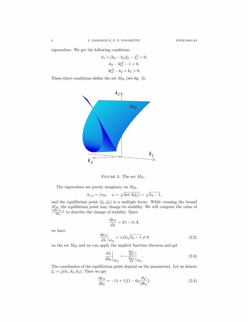
The closure of the set MT divides the parameter space K into two sets M1, M3

M1 = {(k1, k2, k3) ∈ K : k1 = −2ξ31 , k2 < k3 + 3ξ2

1 , ξ1 ∈ R},M3 = {(k1, k2, k3) ∈ K : k1 = −2ξ3

1 , k2 > k3 + 3ξ21 , ξ1 ∈ R}.

The set M1 contsists of all the parameters from K, for which the system (1.1)has a unique equilibrium point (non-saddle), the set M3 consists of those, for whichthe system (1.1) has 3 equilibrium points (non-saddle, saddle, non-saddle). Whilecrossing the boundary MT from the set M3 to M1, two equilibrium points coincideand disappear then. According to Lemma 2.1, the double equilibrium point is asaddle-node. A qualitative local change of the phase portraits occurres, a localbifurcation of codimension 1 - “saddle-node”. �


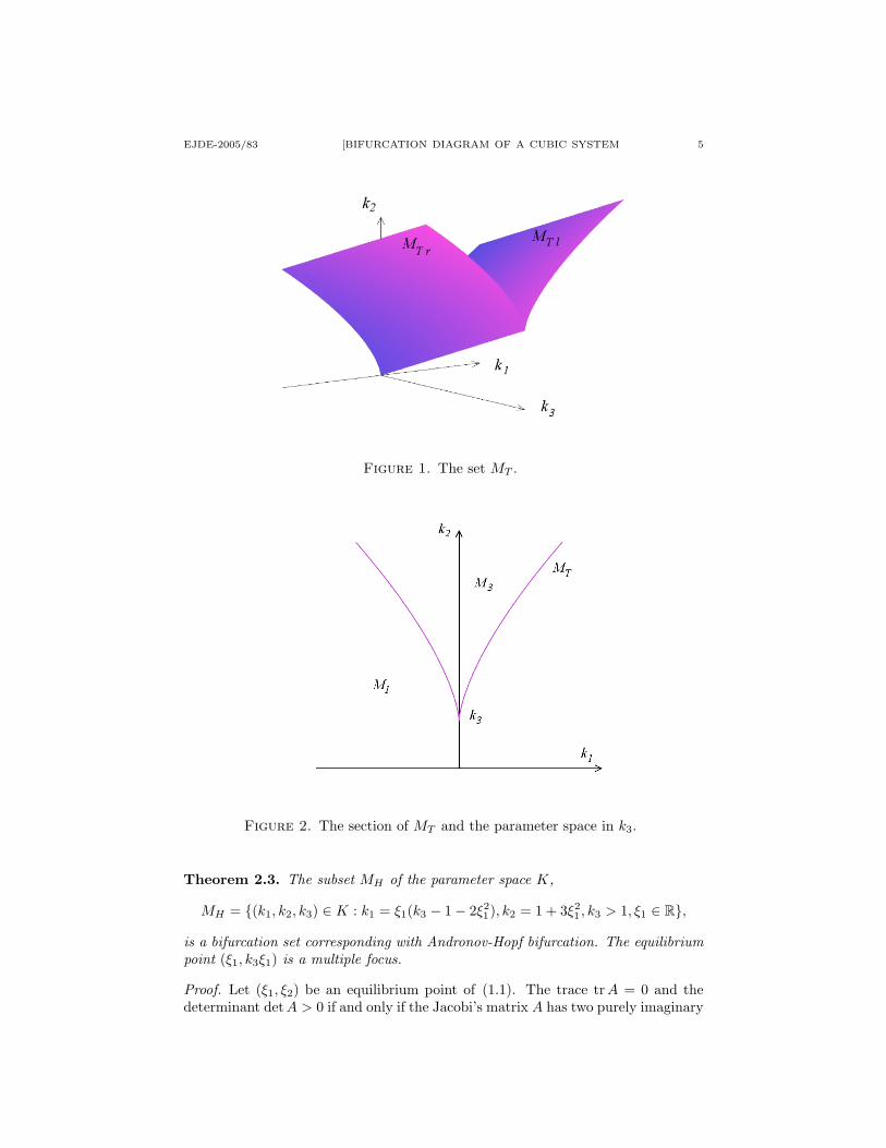
Figure 1. The set MT .

Figure 2. The section of MT and the parameter space in k3.

Theorem 2.3. The subset MH of the parameter space K,

MH = {(k1, k2, k3) ∈ K : k1 = ξ1(k3 − 1− 2ξ21), k2 = 1 + 3ξ2

1 , k3 > 1, ξ1 ∈ R},

is a bifurcation set corresponding with Andronov-Hopf bifurcation. The equilibriumpoint (ξ1, k3ξ1) is a multiple focus.

Proof. Let (ξ1, ξ2) be an equilibrium point of (1.1). The trace trA = 0 and thedeterminant detA > 0 if and only if the Jacobi’s matrix A has two purely imaginary


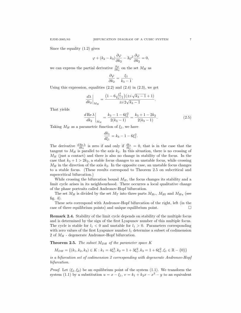
eigenvalues. We get the following conditions

k1 + (k2 − k3)ξ1 − ξ31 = 0,

k2 − 3ξ21 − 1 = 0,

3ξ21 − k2 + k3 > 0.

These three conditions define the set MH (see fig. 3).

Figure 3. The set MH .

The eigenvalues are purely imaginary on MH ,

λ1,2 = ±iω, ω =√

detA(ξ1) =√

k3 − 1,

and the equilibrium point (ξ1, ξ2) is a multiple focus. While crossing the boundMH , the equilibrium point may change its stability. We will compute the value ofd Re λ1,2

dk2to describe the change of stability. Since

dpA

dλ= 2λ− trA,

we havedpA

dλ

∣∣∣MH

= ±i2√

k3 − 1 6= 0 (2.2)

on the set MH and we can apply the implicit function theorem and get

dλ

dk2

∣∣∣∣MH

= −dpA

dk2

dpA

dλ

∣∣∣∣MH

. (2.3)

The coordinates of the equilibrium point depend on the parameters. Let us denoteξ1 = ϕ(k1, k2, k3). Then we get

dpA

dk2= −(λ + 1)

(1− 6ϕ

∂ϕ

∂k2

). (2.4)


Since the equality (1.2) gives

ϕ + (k2 − k3)∂ϕ

∂k2− 3ϕ2 ∂ϕ

∂k2= 0,

we can express the partial derivative ∂ϕ∂k2

on the set MH as

∂ϕ

∂k2=

ξ1

k3 − 1.

Using this expression, equalities (2.2) and (2.4) in (2.3), we get

dλ

dk2

∣∣∣∣MH

=

(1− 6 ξ2

1k3−1

)(±i

√k3 − 1 + 1)

±i 2√

k3 − 1.

That yieldsd Re λ

dk2

∣∣∣∣MH

=k3 − 1− 6ξ2

1

2(k3 − 1)=

k3 + 1− 2k2

2(k3 − 1). (2.5)

Taking MH as a parametric function of ξ1, we have

dk1

dξ1= k3 − 1− 6ξ2

1 .

The derivative d Re λdk2

is zero if and only if dk1dξ1

= 0, that is in the case that thetangent to MH is parallel to the axis k2. In this situation, there is no crossing ofMH (just a contact) and there is also no change in stability of the focus. In thecase that k3 + 1 > 2k2, a stable focus changes to an unstable focus, while crossingMH in the direction of the axis k2. In the opposite case, an unstable focus changesto a stable focus. (These results correspond to Theorem 2.5 on subcritical andsupercritical bifurcation.)

While crossing the bifurcation bound MH , the focus changes its stability and alimit cycle arises in its neighbourhood. There occurres a local qualitative changeof the phase portraits called Andronov-Hopf bifurcation.

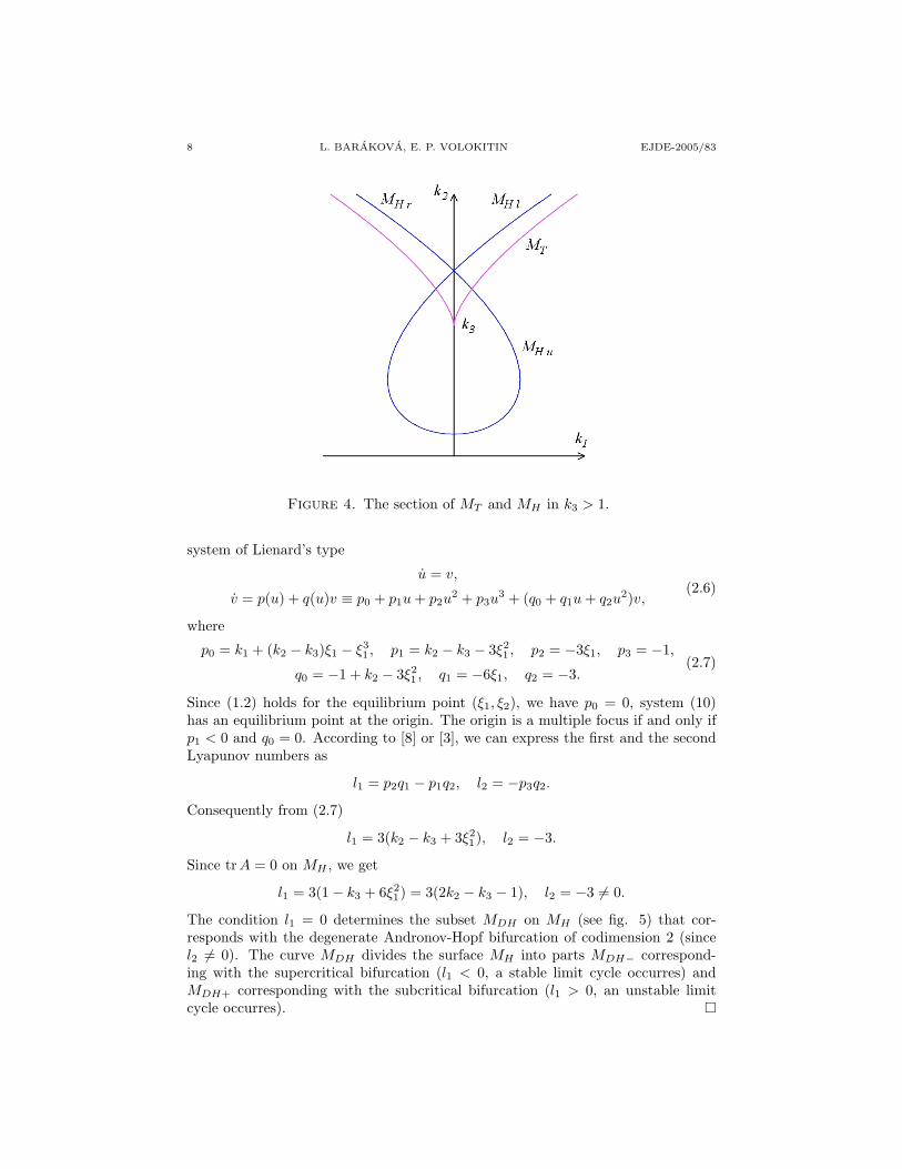
The set MH is divided by the set MT into three parts MHr, MHl and MHu (seefig. 4).

These sets correspond with Andronov-Hopf bifurcation of the right, left (in thecase of three equilibrium points) and unique equilibrium point. �

Remark 2.4. Stability of the limit cycle depends on stability of the multiple focusand is determined by the sign of the first Lyapunov number of this multiple focus.The cycle is stable for l1 < 0 and unstable for l1 > 0. Parameters correspondingwith zero values of the first Lyapunov number l1 determine a subset of codimension2 of MH - degenerate Andronov-Hopf bifurcation.

Theorem 2.5. The subset MDH of the parameter space K

MDH = {(k1, k2, k3) ∈ K : k1 = 4ξ31 , k2 = 1 + 3ξ2

1 , k3 = 1 + 6ξ21 , ξ1 ∈ R− {0}}

is a bifurcation set of codimension 2 corresponding with degenerate Andronov-Hopfbifurcation.

Proof. Let (ξ1, ξ2) be an equilibrium point of the system (1.1). We transform thesystem (1.1) by a substitution u = x− ξ1, v = k1 + k2x− x3 − y to an equivalent


Figure 4. The section of MT and MH in k3 > 1.

system of Lienard’s type

u = v,

v = p(u) + q(u)v ≡ p0 + p1u + p2u2 + p3u

3 + (q0 + q1u + q2u2)v,

(2.6)

where

p0 = k1 + (k2 − k3)ξ1 − ξ31 , p1 = k2 − k3 − 3ξ2

1 , p2 = −3ξ1, p3 = −1,

q0 = −1 + k2 − 3ξ21 , q1 = −6ξ1, q2 = −3.

(2.7)

Since (1.2) holds for the equilibrium point (ξ1, ξ2), we have p0 = 0, system (10)has an equilibrium point at the origin. The origin is a multiple focus if and only ifp1 < 0 and q0 = 0. According to [8] or [3], we can express the first and the secondLyapunov numbers as

l1 = p2q1 − p1q2, l2 = −p3q2.

Consequently from (2.7)

l1 = 3(k2 − k3 + 3ξ21), l2 = −3.

Since trA = 0 on MH , we get

l1 = 3(1− k3 + 6ξ21) = 3(2k2 − k3 − 1), l2 = −3 6= 0.

The condition l1 = 0 determines the subset MDH on MH (see fig. 5) that cor-responds with the degenerate Andronov-Hopf bifurcation of codimension 2 (sincel2 6= 0). The curve MDH divides the surface MH into parts MDH− correspond-ing with the supercritical bifurcation (l1 < 0, a stable limit cycle occurres) andMDH+ corresponding with the subcritical bifurcation (l1 > 0, an unstable limitcycle occurres). �


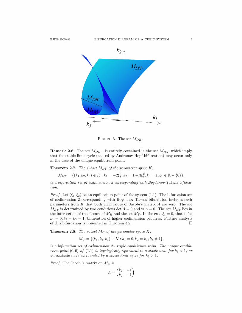
Figure 5. The set MDH .

Remark 2.6. The set MDH− is entirely contained in the set MHu, which implythat the stable limit cycle (caused by Andronov-Hopf bifurcation) may occur onlyin the case of the unique equilibrium point.

Theorem 2.7. The subset MBT of the parameter space K,

MBT = {(k1, k2, k3) ∈ K : k1 = −2ξ31 , k2 = 1 + 3ξ2

1 , k3 = 1, ξ1 ∈ R− {0}},

is a bifurcation set of codimension 2 corresponding with Bogdanov-Takens bifurca-tion.

Proof. Let (ξ1, ξ2) be an equilibrium point of the system (1.1). The bifurcation setof codimension 2 corresponding with Bogdanov-Takens bifurcation includes suchparameters from K that both eigenvalues of Jacobi’s matrix A are zero. The setMBT is determined by two conditions detA = 0 and tr A = 0. The set MBT lies inthe intersection of the closure of MH and the set MT . In the case ξ1 = 0, that is fork1 = 0, k2 = k3 = 1, bifurcation of higher codimension occurres. Further analysisof this bifurcation is presented in Theorem 3.2. �

Theorem 2.8. The subset MC of the parameter space K,

MC = {(k1, k2, k3) ∈ K : k1 = 0, k2 = k3, k3 6= 1},

is a bifurcation set of codimension 2 - triple equilibrium point. The unique equilib-rium point (0, 0) of (1.1) is topologically equivalent to a stable node for k3 < 1, oran unstable node surrounded by a stable limit cycle for k3 > 1.

Proof. The Jacobi’s matrix on MC is

A =(

k2 −1k2 −1

)


and its eigenvalues are λ1 = 0 and λ2 = k2−1. The origin is the unique equilibriumpoint of (1.1) and it is stable for k3 < 1, unstable for k3 > 1. The unstableunique equilibrium is surrounded by a stable limit cycle according to Lemma 1.1on existence of a globally attractive set and the Poincare’s theorem. The origin istopologically equivalent to a node according to Lemma 2.1. �

3. Non-local bifurcations

In contradiction to local bifurcations, where the bifurcation sets could be ex-pressed explicitly, bifurcation sets corresponding with non-local bifurcations canonly be studied numerically or can be approximated with accuracy to a particularorder in the neighbourhood of some important bifurcation points.

Non-local bifurcation of codimension 1 - multiple cycle. The curve MDH

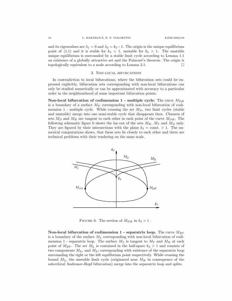
is a boundary of a surface MD corresponding with non-local bifurcation of codi-mension 1 - multiple cycle. While crossing the set MD, two limit cycles (stableand unstable) merge into one semi-stable cycle that disappears then. Closures ofsets MD and MH are tangent to each other in each point of the curve MDH . Thefollowing schematic figure 6 shows the lay-out of the sets MH , MT and MD only.They are figured by their intersections with the plane k3 = const. > 1. The nu-merical computations shows, that these sets lie closely to each other and there aretechnical problems with their rendering on the same scale.

Figure 6. The section of MDH in k3 > 1 .

Non-local bifurcation of codimension 1 - separatrix loop. The curve MBT

is a boundary of the surface ML corresponding with non-local bifurcation of codi-mension 1 - separatrix loop. The surface ML is tangent to MT and MH at eachpoint of MBT . The set ML is contained in the half-space k3 > 1 and consists oftwo components MLr and MLl corresponding with existence of the separatrix loopsurrounding the right or the left equilibrium point respectively. While crossing thebound ML, the unstable limit cycle (originated near MH in consequence of thesubcritical Andronov-Hopf bifurcation) merge into the separatrix loop and splits.


Let (ξ1, ξ2) be the right double equilibrium point of the system (1.1). Then theparameters of the system (1.1) lie in the set MBT (Bogdanov-Takens bifurcation)and the coordinates of the double equilibrium point satisfy

ξ1 =

√k2 − 1

3, ξ2 = k3

√k2 − 1

3according to Theorem 2.7. Using the following substitution

x = x1 −√

k2 − 13

, y = x2 − k3

√k2 − 1

3,

we transform the system (1.1) into a system

x = k1 +

√k2 − 1

3

(k2 − k3 −

k2 − 13

)+ x−

√3(k2 − 1)x2 − x3 − y,

y = k3x− y.

(3.1)

The origin is a double equilibrium point of the system (12) with two zero eigenvaluesfor parameters from MBT .

System (3.1) can be transformed by the linear transformation x1 = y, x2 =k3x− y into the system

x1 = x2,

x2 = h00 + h10x1 +12h20x

21 + h11x1x2 +

12h02x

22 + R(x1, x2, k1, k2, k3),

(3.2)

where

h00 = k3

(k1 +

√k2 − 1

3(k2 − k3 −

k2 − 13

)), h10 = 1− k3,

h20 = − 2k3

√3(k2 − 1), h11 = − 2

k3

√3(k2 − 1),

h02 = − 2k3

√3(k2 − 1), R(x1, x2, k1, k2, k3) = − (x1 + x2)3

k23

.

This transformation keeps the equilibrium point at the origin as well as its zeroeigenvalues. In the further analysis, we will study system (3.2) instead of theequivalent system (1.1).

Remark 3.1. For (k1, k2, k3) ∈ MBT , the following statements hold

h00 = 0, h10 = 0, h11 = h20 = h02 6= 0.

Theorem 3.2. The system (3.2) can be transformed by a smooth non-degeneratechange of parameters to the Bogdanov-Takens normal canonical form

x1 = x2,

x2 = β1 + β2x1 + x21 + x1x2 + O(‖x‖3),

(3.3)

where

β1 =h11

(−h10 + 14h02h00 + 1

2 )3h00,

β2 =1

(−h10 + 14h02h00 + 1

2 )2(h10 − h00h02).

(3.4)


In the neighbourhood of the Bogdanov-Takens curve MBT corresponding with theright double equilibrium point, the set MLr can be expressed at the form

MLr ={(k1, k2, k3) ∈ R3 : β2 < 0, β1 = − 6

25β2

2 + o(β22)

}. (3.5)

The set MLl is symmetrical to MLr according to the plane k1 = 0.

Proof. The change of time dt = (1− h022 x1)dτ and the substitution

u1 = x1, u2 = x2 −h02

2x1x2

eliminates the term with x22. We get a system of the form

u1 = u2,

u2 = ν1 + ν2u1 + C1u21 + C2u1u2 + O(‖u‖3),

where

ν1 = h00, ν2 = h10 − h00h02, C1 = −h02h10 +14h2

02h00 +12h20, C2 = h11.

Note that C1 = 12h20 6= 0 on MBT according to Remark 3.1. Introducing a new

time (denoted again with t)

t =∣∣C2

C1

∣∣τand new variables (denoted again with x1 and x2)

x1 =C2

2

C1u1, x2 = sgn

(C2

C1

)C32

C21

u2,

we get the Bogdanov-Takens normal canonical form (3.3), where

β1 =h4

11

(−h02h10 + 14h2

02h00 + 12h20)3

h00,

β2 =h2

11

(−h02h10 + 14h2

02h00 + 12h20)2

(h10 − h00h02).

With respect to the fact that h20 = h11 = h02, we get the expressions (3.4).The coefficient of the term with x1x2 corresponds to

s = sgn(C2

C1

)∣∣MBT

= sgn( h11

−h02h10 + 14h2

02h00 + 12h20

)∣∣MBT

.

According to Remark 3.1, we have s = sgn 2 = 1. The Bogdanov-Takens bifurcationis non-degenerate, since

h11 = −2√

3(k2 − 1) = −6ξ1 6= 0

and h20 6= 0 on MBT . The change of parameters is invertible in the neighbour-hood of the origin. It can be verified by a direct computation of the followingdeterminants and finding∣∣∣∣∣∂β1

∂k1

∂β1∂k2

∂β2∂k1

∂β2∂k2

∣∣∣∣∣ 6= 0,

∣∣∣∣∣∂β1∂k2

∂β1∂k3

∂β2∂k2

∂β2∂k3

∣∣∣∣∣ 6= 0,

∣∣∣∣∣∂β1∂k3

∂β1∂k1

∂β2∂k3

∂β2∂k1

∣∣∣∣∣ 6= 0.

This fact implies that the change of parameters cause no degeneration of the bifur-cation manifold according to the parameter space. (In the bifurcation theory thisregularity of the parameter transformation is called the transversality condition.)


The expression for the set ML can be found in [6, Theorem 8.5, Appendix] or in[4]. The set MLl has to be symmetric to MLr about to the plane k1 = 0. �

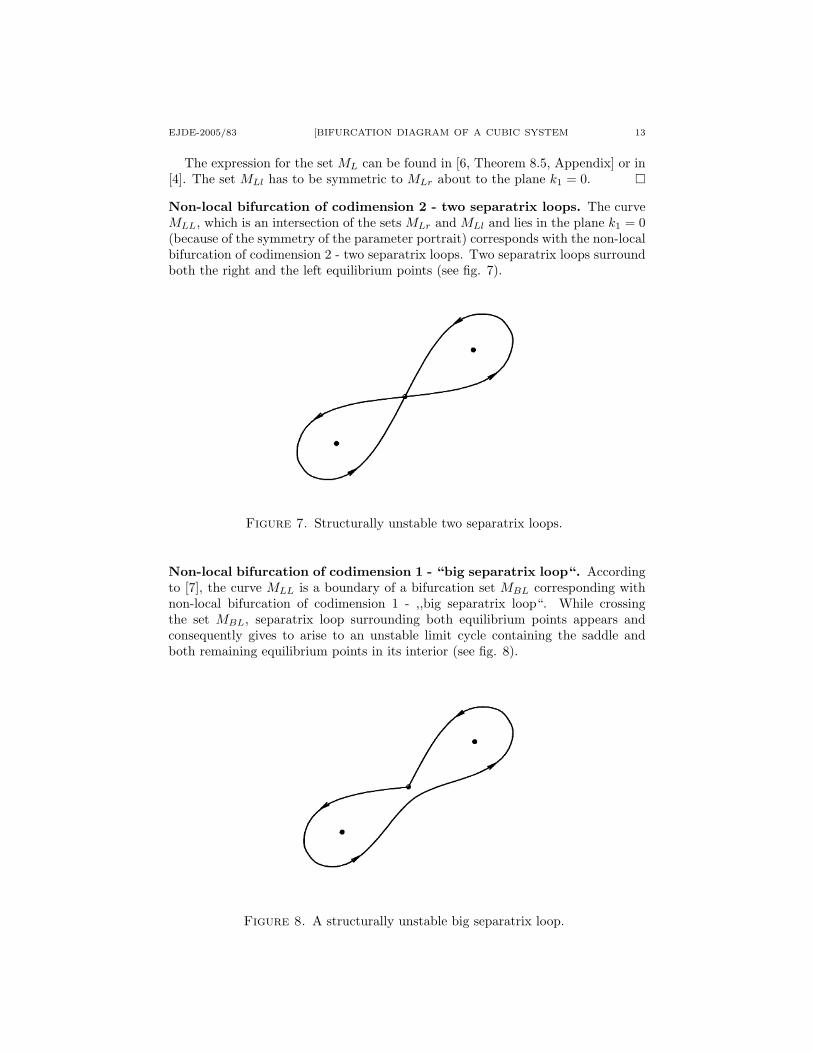
Non-local bifurcation of codimension 2 - two separatrix loops. The curveMLL, which is an intersection of the sets MLr and MLl and lies in the plane k1 = 0(because of the symmetry of the parameter portrait) corresponds with the non-localbifurcation of codimension 2 - two separatrix loops. Two separatrix loops surroundboth the right and the left equilibrium points (see fig. 7).

Figure 7. Structurally unstable two separatrix loops.

Non-local bifurcation of codimension 1 - “big separatrix loop“. Accordingto [7], the curve MLL is a boundary of a bifurcation set MBL corresponding withnon-local bifurcation of codimension 1 - ,,big separatrix loop“. While crossingthe set MBL, separatrix loop surrounding both equilibrium points appears andconsequently gives to arise to an unstable limit cycle containing the saddle andboth remaining equilibrium points in its interior (see fig. 8).

Figure 8. A structurally unstable big separatrix loop.


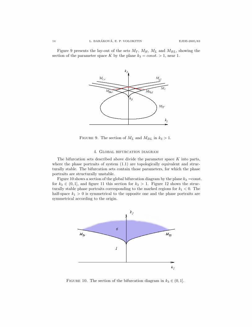
Figure 9 presents the lay-out of the sets MT , MH , ML and MBL, showing thesection of the parameter space K by the plane k3 = const. > 1, near 1.

Figure 9. The section of ML and MBL in k3 > 1.

4. Global bifurcation diagram

The bifurcation sets described above divide the parameter space K into parts,where the phase portraits of system (1.1) are topologically equivalent and struc-turally stable. The bifurcation sets contain those parameters, for which the phaseportraits are structurally unstable.

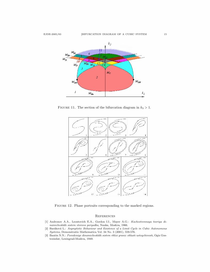
Figure 10 shows a section of the global bifurcation diagram by the plane k3 =const.for k3 ∈ (0, 1], and figure 11 this section for k3 > 1. Figure 12 shows the struc-turally stable phase portraits corresponding to the marked regions for k1 < 0. Thehalf-space k1 > 0 is symmetrical to the opposite one and the phase portraits aresymmetrical according to the origin.

Figure 10. The section of the bifurcation diagram in k3 ∈ (0, 1].


Figure 11. The section of the bifurcation diagram in k3 > 1.

Figure 12. Phase portraits corresponding to the marked regions.

References

[1] Andronov A.A., Leontovich E.A., Gordon I.I., Mayer A.G.: Kachestvennaya teoriya di-namicheskikh sistem vtorovo poryadka, Nauka, Moskva, 1966.

[2] Barakova L.: Asymptotic Behaviour and Existence of a Limit Cycle in Cubic Autonomous

Systems, Demonstratio Mathematica Vol. 34 No. 3 (2001), 559-576.[3] Bautin N.N.: Povedeniye dinamicheskikh sistem vblizi granic oblasti ustoychivosti, Ogiz Gos-

texizdat, Leningrad-Moskva, 1949.


[4] Bogdanov R.I.: Versalnaya deformatsiya osoboy tochki vektornovo polya na ploskosti v

sluchae nulevikh sobstvennikh chisel, Tr. sem. im. Petrovskovo, No. 2 (1976), 37-65.

[5] Kaldor N.: A Model of the Trade Cycle, Econ. Jour. 50 (1940), 78-92.[6] Kuznetsov Y.A., Elements of Applied Bifucation Theory, Second Edition, Applied Mathe-

matical Sciences 112, Berlin, Heidelgerg, New York, Springer-Verlag, 1995, 1998.

[7] Turaev D.V.: ,,Bifurkatsii dvumernikh dinamicheskikh sistem, blizkich k sisteme s dvumyapetlyami separatris“, Uspechi mat. nauk Vol. 40, No. 6 (1985), 203-204.

[8] Volokitin E.P., Treskov S.A.: Bifurkatsionnaya diagramma kubicheskoy sistemi Lienar-

dovskovo tipa, Sibirskij zhurnal industrialnoy matematiki Vol. 5, No. 3(11) (2002), 67-75.

Lenka Barakova

Mendel University, Dept. of Math., Zemedelska 1, 613 00 Brno, Czech Rep.

E-mail address: [email protected]

Evgenii P. Volokitin

Sobolev Institute of Mathematics, Novosibirsk, 630090, RussiaE-mail address: [email protected]

electronic journal of diﬀerential equations, … journal of diﬀerential equations, vol....

Documents