Electricity consumption, education expenditure and economic growth

in Chinese cities

Zheng Fang, Yang Chen*

Presented at IAEE, Singapore

June 19-21, 2017

1

Outline of the paper

• Introduction

—motivation

—research questions

—contribution

• Data and descriptive evidence

• Theoretical framework and empirical methods

• Main results

• Conclusion

2

Motivation

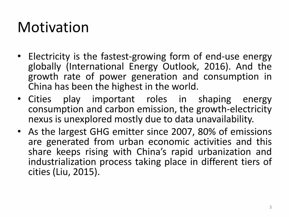
• Electricity is the fastest-growing form of end-use energy globally (International Energy Outlook, 2016). And the growth rate of power generation and consumption in China has been the highest in the world.

• Cities play important roles in shaping energy consumption and carbon emission, the growth-electricity nexus is unexplored mostly due to data unavailability.

• As the largest GHG emitter since 2007, 80% of emissions are generated from urban economic activities and this share keeps rising with China’s rapid urbanization and industrialization process taking place in different tiers of cities (Liu, 2015).

3

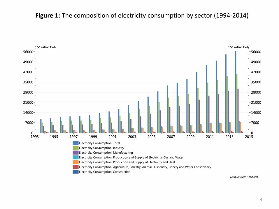
Data Source: Wind Info

Electricity Consumption: Total

Electricity Consumption: Industry

Electricity Consumption: Manufacturing

Electricity Consumption: Production and Supply of Electricity, Gas and Water

Electricity Consumption: Production and Supply of Electricity and Heat

Electricity Consumption: Agriculture, Forestry, Animal Husbandry, Fishery and Water Conservancy

Electricity Consumption: Construction

1993 1995 1997 1999 2001 2003 2005 2007 2009 2011 2013 201519930 0

7000 7000

14000 14000

21000 21000

28000 28000

35000 35000

42000 42000

49000 49000

56000 56000

100 million kwh 100 million kwh100 million kwh 100 million kwh

Figure 1: The composition of electricity consumption by sector (1994-2014)

4

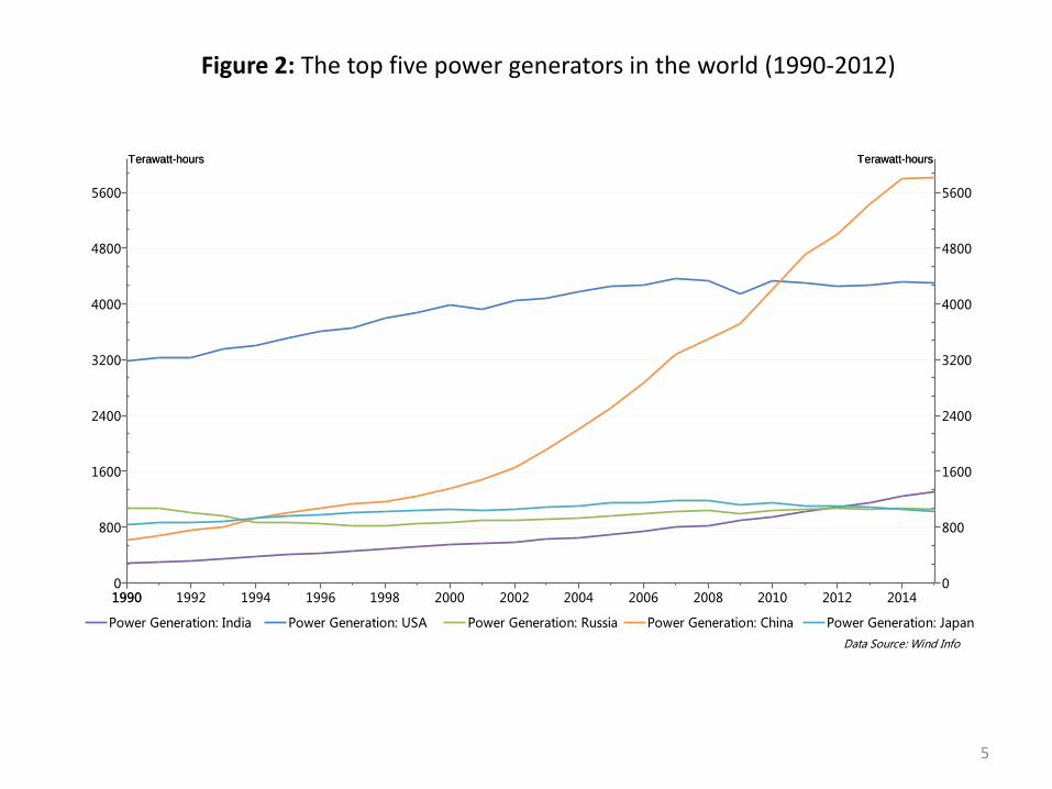
Data Source: Wind Info

Power Generation: India Power Generation: USA Power Generation: Russia Power Generation: China Power Generation: Japan

1990 1992 1994 1996 1998 2000 2002 2004 2006 2008 2010 2012 201419900 0

800 800

1600 1600

2400 2400

3200 3200

4000 4000

4800 4800

5600 5600

Terawatt-hours Terawatt-hoursTerawatt-hours Terawatt-hours

Figure 2: The top five power generators in the world (1990-2012)

5

Data Source: Wind Info

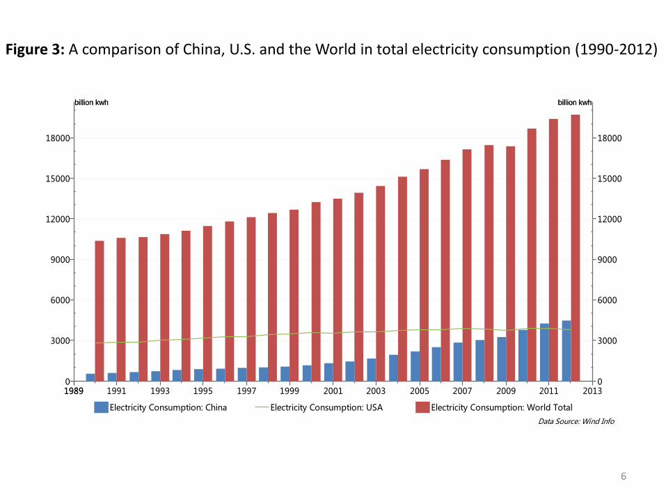
Electricity Consumption: China Electricity Consumption: USA Electricity Consumption: World Total

1989 1991 1993 1995 1997 1999 2001 2003 2005 2007 2009 2011 201319890 0

3000 3000

6000 6000

9000 9000

12000 12000

15000 15000

18000 18000

billion kwh billion kwhbillion kwh billion kwh

Figure 3: A comparison of China, U.S. and the World in total electricity consumption (1990-2012)

6

Data Source: Wind Info

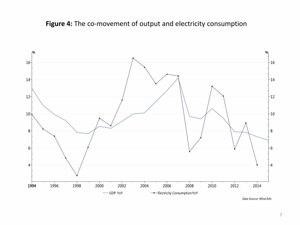
GDP: YoY Electricity Consumption:YoY

1994 1996 1998 2000 2002 2004 2006 2008 2010 2012 20141994

4 4

6 6

8 8

10 10

12 12

14 14

16 16

% %% %

Figure 4: The co-movement of output and electricity consumption

7

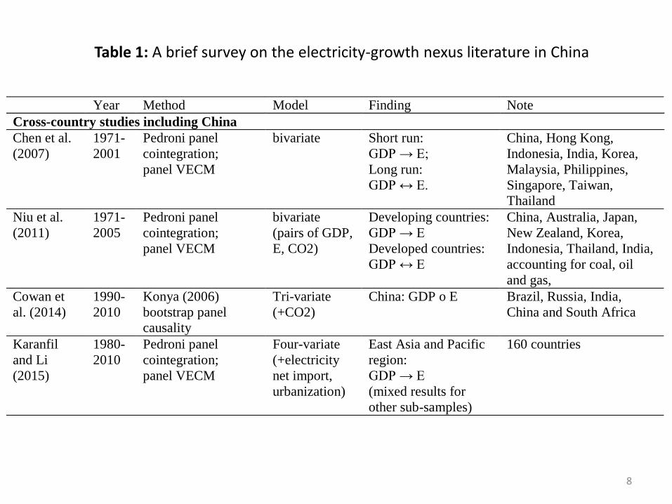
Year Method Model Finding Note

Cross-country studies including China

Chen et al.

(2007)

1971-

2001

Pedroni panel

cointegration;

panel VECM

bivariate Short run:

GDP → E;

Long run:

GDP ↔ E.

China, Hong Kong,

Indonesia, India, Korea,

Malaysia, Philippines,

Singapore, Taiwan,

Thailand

Niu et al.

(2011)

1971-

2005

Pedroni panel

cointegration;

panel VECM

bivariate

(pairs of GDP,

E, CO2)

Developing countries:

GDP → E

Developed countries:

GDP ↔ E

China, Australia, Japan,

New Zealand, Korea,

Indonesia, Thailand, India,

accounting for coal, oil

and gas,

Cowan et

al. (2014)

1990-

2010

Konya (2006)

bootstrap panel

causality

Tri-variate

(+CO2)

China: GDP o E Brazil, Russia, India,

China and South Africa

Karanfil

and Li

(2015)

1980-

2010

Pedroni panel

cointegration;

panel VECM

Four-variate

(+electricity

net import,

urbanization)

East Asia and Pacific

region:

GDP → E

(mixed results for

other sub-samples)

160 countries

Table 1: A brief survey on the electricity-growth nexus literature in China

8

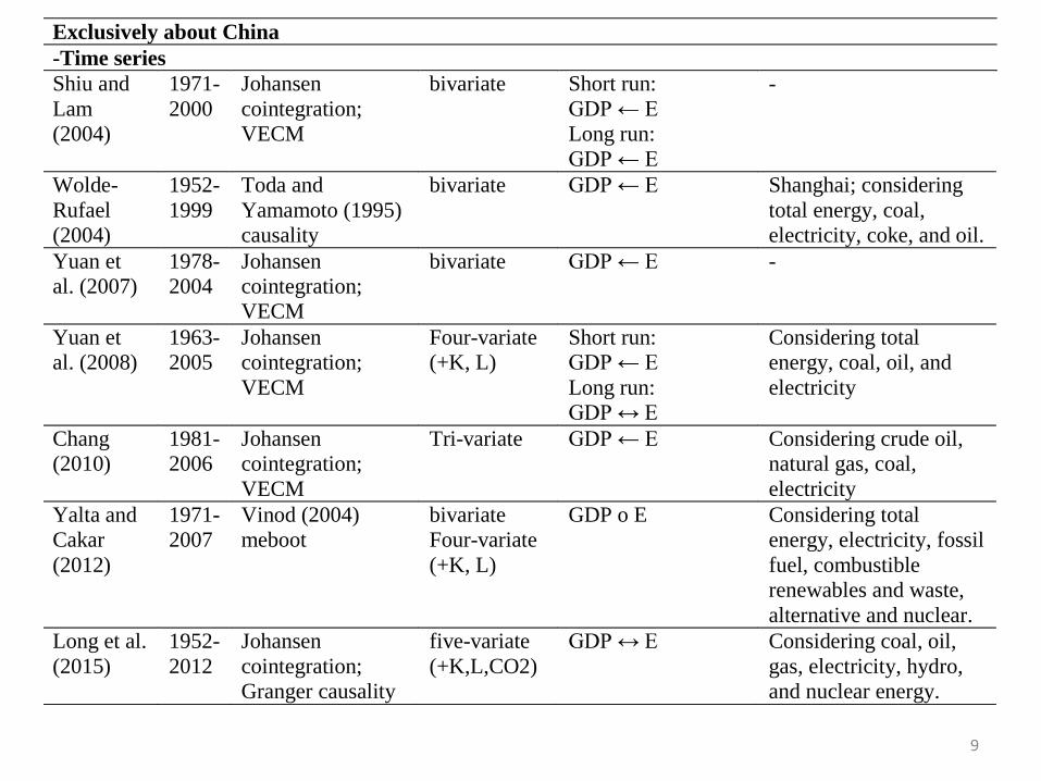
Exclusively about China

-Time series

Shiu and

Lam

(2004)

1971-

2000

Johansen

cointegration;

VECM

bivariate Short run:

GDP ← E

Long run:

GDP ← E

-

Wolde-

Rufael

(2004)

1952-

1999

Toda and

Yamamoto (1995)

causality

bivariate GDP ← E Shanghai; considering

total energy, coal,

electricity, coke, and oil.

Yuan et

al. (2007)

1978-

2004

Johansen

cointegration;

VECM

bivariate GDP ← E -

Yuan et

al. (2008)

1963-

2005

Johansen

cointegration;

VECM

Four-variate

(+K, L)

Short run:

GDP ← E

Long run:

GDP ↔ E

Considering total

energy, coal, oil, and

electricity

Chang

(2010)

1981-

2006

Johansen

cointegration;

VECM

Tri-variate GDP ← E Considering crude oil,

natural gas, coal,

electricity

Yalta and

Cakar

(2012)

1971-

2007

Vinod (2004)

meboot

bivariate

Four-variate

(+K, L)

GDP o E Considering total

energy, electricity, fossil

fuel, combustible

renewables and waste,

alternative and nuclear.

Long et al.

(2015)

1952-

2012

Johansen

cointegration;

Granger causality

five-variate

(+K,L,CO2)

GDP ↔ E Considering coal, oil,

gas, electricity, hydro,

and nuclear energy.

9

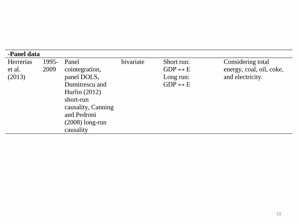
-Panel data

Herrerias

et al.

(2013)

1995-

2009

Panel

cointegration,

panel DOLS,

Dumitrescu and

Hurlin (2012)

short-run

causality, Canning

and Pedroni

(2008) long-run

causality

bivariate Short run:

GDP ↔ E

Long run:

GDP ↔ E

Considering total

energy, coal, oil, coke,

and electricity.

10

Research questions

• What are the impacts of electricity consumption and human capital on city economic growth?

• Are the impacts homogeneous across regions and city tiers?

• What are the causal relations between electricity consumption and growth of cities?

11

Contribution

• Focus on the growth-electricity nexus exclusively in China, accounting for commonly observed cross-sectional dependence and heterogeneity of causal relations using city-level panel data.

• Adopt the multi-variable framework in the energy-augmented neoclassical production function including human capital.

• Apply the continuously updated fully-modified estimator to investigate the magnitude and elasticity of the covariates with regard to economic growth and extend the analysis to different groups of cities classified by three macro regions and by city tiers.

12

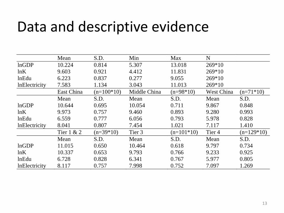
Data and descriptive evidence

Mean S.D. Min Max N

lnGDP 10.224 0.814 5.307 13.018 269*10

lnK 9.603 0.921 4.412 11.831 269*10

lnEdu 6.223 0.837 0.277 9.055 269*10

lnElectricity 7.583 1.134 3.043 11.013 269*10

East China (n=100*10) Middle China (n=98*10) West China (n=71*10)

Mean S.D. Mean S.D. Mean S.D.

lnGDP 10.644 0.695 10.054 0.711 9.867 0.848

lnK 9.973 0.757 9.460 0.893 9.280 0.993

lnEdu 6.559 0.777 6.056 0.793 5.978 0.828

lnElectricity 8.041 0.807 7.454 1.021 7.117 1.410

Tier 1 & 2 (n=39*10) Tier 3 (n=101*10) Tier 4 (n=129*10)

Mean S.D. Mean S.D. Mean S.D.

lnGDP 11.015 0.650 10.464 0.618 9.797 0.734

lnK 10.337 0.653 9.793 0.766 9.233 0.925

lnEdu 6.728 0.828 6.341 0.767 5.977 0.805

lnElectricity 8.117 0.757 7.998 0.752 7.097 1.269

13

0

1000

2000

3000

4000

5000

6000

2003 2004 2005 2006 2007 2008 2009 2010 2011 2012

East Middle West

0

1000

2000

3000

4000

5000

6000

2003 2004 2005 2006 2007 2008 2009 2010 2011 2012

Tier 1 Tier 2 Tier 3 Tier 4

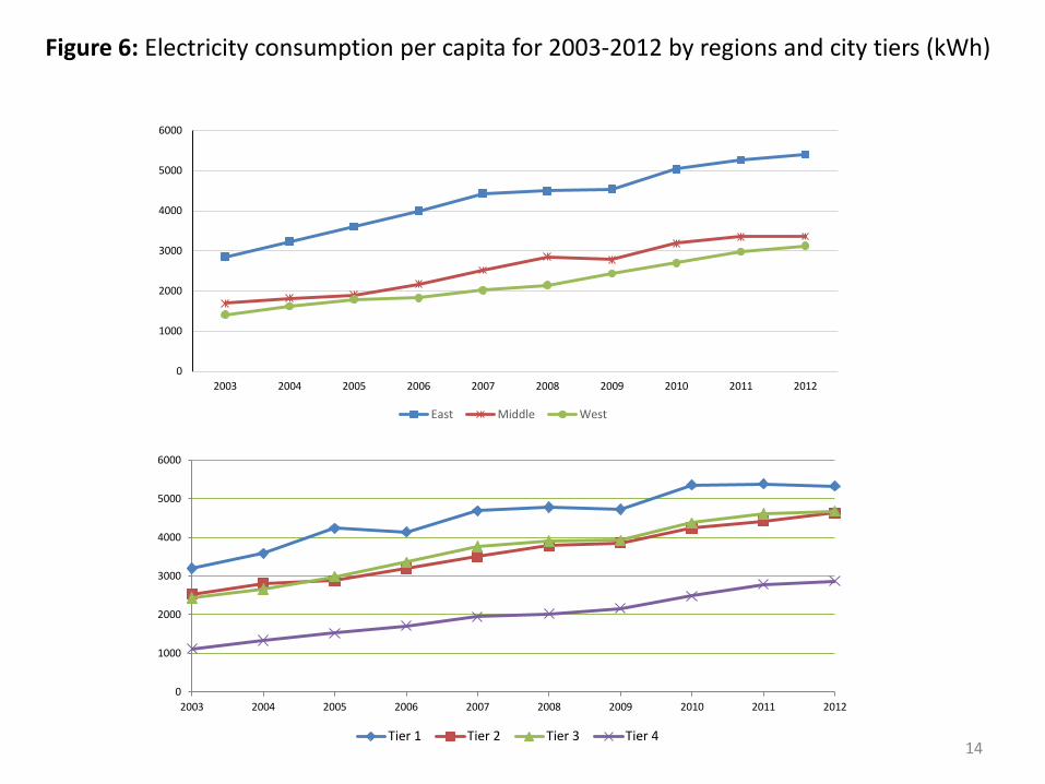
Figure 6: Electricity consumption per capita for 2003-2012 by regions and city tiers (kWh)

14

-

20,000

40,000

60,000

80,000

100,000

120,000

140,000

160,000

180,000

200,000

2003 2004 2005 2006 2007 2008 2009 2010 2011 2012

Tier 1 Tier 2 Tier 3 Tier 4

-

20,000

40,000

60,000

80,000

100,000

120,000

2003 2004 2005 2006 2007 2008 2009 2010 2011 2012

East Middle West

Figure 7: Output per capita for 2003-2012 by regions and city tiers (yuan)

15

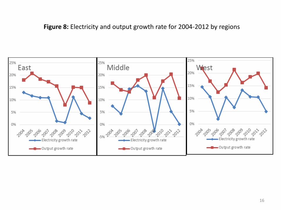
Figure 8: Electricity and output growth rate for 2004-2012 by regions

16

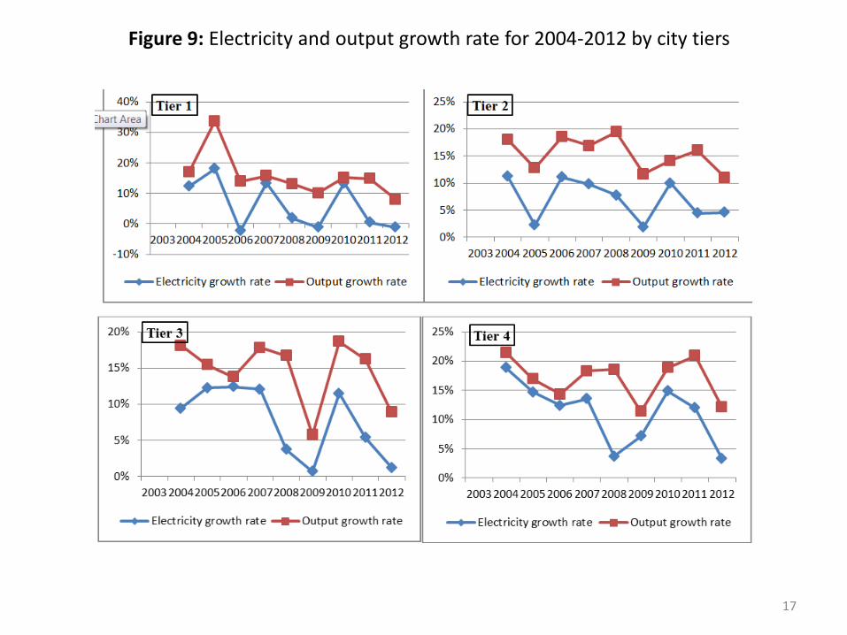
Figure 9: Electricity and output growth rate for 2004-2012 by city tiers

17

Beijing

Tianjin

Shanghai

Guangzhou City

Shenzhen City

.14

.16

.18

.2.2

2

grow

th o

f out

put (

%)

.07 .08 .09 .1 .11growth of electricity consumption (%)

Shijiazhuang City

Tangshan City

Taiyuan City

Hohhot City

Baotou City

Shenyang CityDalian City

Changchun City

Harbin City

Nanjing City

Wuxi City

Suzhou City

Hangzhou City

Ningbo City

Hefei City

Fuzhou City

Xiamen CityQuanzhou City

Nanchang City

Ji'nan City

Qingdao CityYantai CityZhengzhou City

Wuhan City

Changsha City

Foshan City

Dongguan City

Nanning City

Chongqing

Chengdu City

Guiyang City

Kunming City

Xi'an City

Lanzhou City

Urumqi City

.1.1

5.2

.25

grow

th o

f out

put (

%)

0 .05 .1 .15 .2 .25growth of electricity consumption (%)

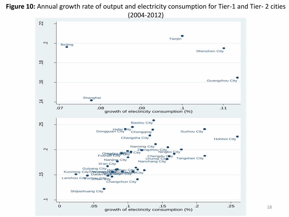
Figure 10: Annual growth rate of output and electricity consumption for Tier-1 and Tier- 2 cities (2004-2012)

18

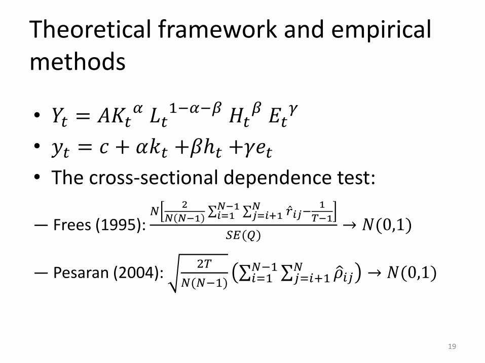
Theoretical framework and empirical methods

• 𝑌𝑡 = 𝐴𝐾𝑡𝛼 𝐿𝑡

1−𝛼−𝛽 𝐻𝑡𝛽 𝐸𝑡

𝛾

• 𝑦𝑡 = 𝑐 + 𝛼𝑘𝑡 +𝛽ℎ𝑡 +𝛾𝑒𝑡

• The cross-sectional dependence test:

— Frees (1995): 𝑁

2

𝑁 𝑁−1 𝑟 𝑖𝑗

𝑁𝑗=𝑖+1

𝑁−1𝑖=1 −

1

𝑇−1

𝑆𝐸(𝑄)→ 𝑁(0,1)

— Pesaran (2004): 2𝑇

𝑁(𝑁−1) 𝜌 𝑖𝑗

𝑁𝑗=𝑖+1

𝑁−1𝑖=1 → 𝑁(0,1)

19

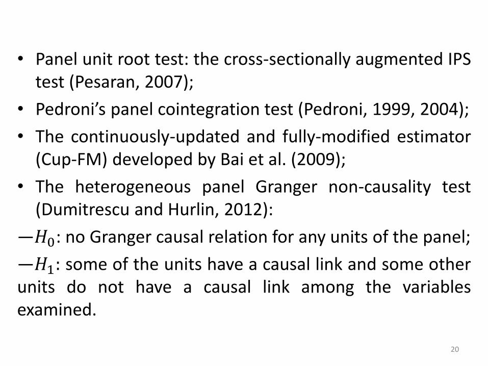
• Panel unit root test: the cross-sectionally augmented IPS test (Pesaran, 2007);

• Pedroni’s panel cointegration test (Pedroni, 1999, 2004);

• The continuously-updated and fully-modified estimator (Cup-FM) developed by Bai et al. (2009);

• The heterogeneous panel Granger non-causality test (Dumitrescu and Hurlin, 2012):

—𝐻0: no Granger causal relation for any units of the panel;

—𝐻1: some of the units have a causal link and some other units do not have a causal link among the variables examined.

20

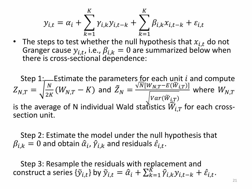
𝑦𝑖,𝑡 = 𝛼𝑖 + 𝛾𝑖,𝑘𝑦𝑖,𝑡−𝑘

𝐾

𝑘=1

+ 𝛽𝑖,𝑘𝑥𝑖,𝑡−𝑘

𝐾

𝑘=1

+ 𝜀𝑖,𝑡

• The steps to test whether the null hypothesis that 𝑥𝑖,𝑡 do not Granger cause 𝑦𝑖,𝑡, i.e., 𝛽𝑖,𝑘 = 0 are summarized below when there is cross-sectional dependence:

Step 1: Estimate the parameters for each unit 𝑖 and compute

𝑍𝑁,𝑇 =𝑁

2𝐾(𝑊𝑁,𝑇 − 𝐾) and 𝑍 𝑁 =

𝑁[𝑊𝑁,𝑇−𝐸(𝑊 𝑖,𝑇)]

𝑉𝑎𝑟(𝑊 𝑖,𝑇) where 𝑊𝑁,𝑇

is the average of N individual Wald statistics 𝑊 𝑖,𝑇 for each cross-section unit. Step 2: Estimate the model under the null hypothesis that 𝛽𝑖,𝑘 = 0 and obtain 𝛼 𝑖, 𝛾 𝑖,𝑘 and residuals 𝜀 𝑖,𝑡. Step 3: Resample the residuals with replacement and construct a series {𝑦 𝑖,𝑡} by 𝑦 𝑖,𝑡 = 𝛼 𝑖 + 𝛾 𝑖,𝑘𝑦𝑖,𝑡−𝑘

𝐾𝑘=1 + 𝜀 𝑖,𝑡.

21

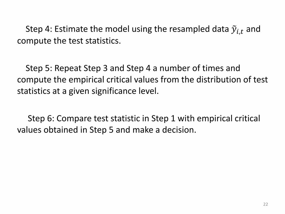
Step 4: Estimate the model using the resampled data 𝑦 𝑖,𝑡 and compute the test statistics.

Step 5: Repeat Step 3 and Step 4 a number of times and compute the empirical critical values from the distribution of test statistics at a given significance level.

Step 6: Compare test statistic in Step 1 with empirical critical values obtained in Step 5 and make a decision.

22

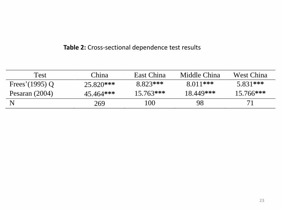
Test China East China Middle China West China

Frees’(1995) Q 25.820*** 8.823*** 8.011*** 5.831***

Pesaran (2004) 45.464*** 15.763*** 18.449*** 15.766***

N 269 100 98 71

Table 2: Cross-sectional dependence test results

23

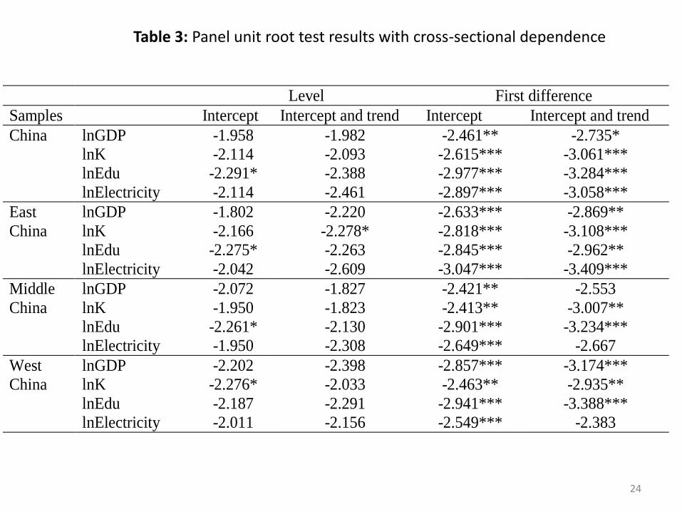
Level First difference

Samples Intercept Intercept and trend Intercept Intercept and trend

China lnGDP -1.958 -1.982 -2.461** -2.735*

lnK -2.114 -2.093 -2.615*** -3.061***

lnEdu -2.291* -2.388 -2.977*** -3.284***

lnElectricity -2.114 -2.461 -2.897*** -3.058***

East

China

lnGDP -1.802 -2.220 -2.633*** -2.869**

lnK -2.166 -2.278* -2.818*** -3.108***

lnEdu -2.275* -2.263 -2.845*** -2.962**

lnElectricity -2.042 -2.609 -3.047*** -3.409***

Middle

China

lnGDP -2.072 -1.827 -2.421** -2.553

lnK -1.950 -1.823 -2.413** -3.007**

lnEdu -2.261* -2.130 -2.901*** -3.234***

lnElectricity -1.950 -2.308 -2.649*** -2.667

West

China

lnGDP -2.202 -2.398 -2.857*** -3.174***

lnK -2.276* -2.033 -2.463** -2.935**

lnEdu -2.187 -2.291 -2.941*** -3.388***

lnElectricity -2.011 -2.156 -2.549*** -2.383

Table 3: Panel unit root test results with cross-sectional dependence

24

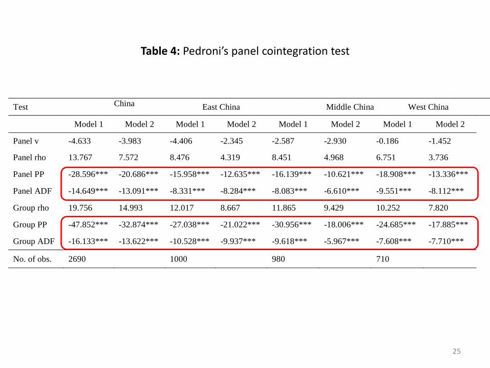
Test China East China Middle China West China

Model 1 Model 2 Model 1 Model 2 Model 1 Model 2 Model 1 Model 2

Panel v -4.633 -3.983 -4.406 -2.345 -2.587 -2.930 -0.186 -1.452

Panel rho 13.767 7.572 8.476 4.319 8.451 4.968 6.751 3.736

Panel PP -28.596*** -20.686*** -15.958*** -12.635*** -16.139*** -10.621*** -18.908*** -13.336***

Panel ADF -14.649*** -13.091*** -8.331*** -8.284*** -8.083*** -6.610*** -9.551*** -8.112***

Group rho 19.756 14.993 12.017 8.667 11.865 9.429 10.252 7.820

Group PP -47.852*** -32.874*** -27.038*** -21.022*** -30.956*** -18.006*** -24.685*** -17.885***

Group ADF -16.133*** -13.622*** -10.528*** -9.937*** -9.618*** -5.967*** -7.608*** -7.710***

No. of obs. 2690 1000 980 710

Table 4: Pedroni’s panel cointegration test

25

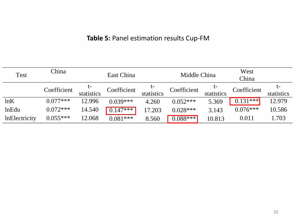
Test China

East China Middle China West

China

Coefficient t-

statistics Coefficient

t-

statistics Coefficient

t-

statistics Coefficient

t-

statistics

lnK 0.077*** 12.996 0.039*** 4.260 0.052*** 5.369 0.131*** 12.979

lnEdu 0.072*** 14.540 0.147*** 17.203 0.028*** 3.143 0.076*** 10.586

lnElectricity 0.055*** 12.068 0.081*** 8.560 0.088*** 10.813 0.011 1.703

Table 5: Panel estimation results Cup-FM

26

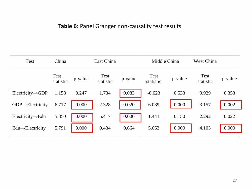
Test China

East China Middle China West China

Test

statistic p-value

Test

statistic p-value

Test

statistic p-value

Test

statistic p-value

Electricity→GDP 1.158 0.247 1.734 0.083 -0.623 0.533 0.929 0.353

GDP→Electricity 6.717 0.000 2.328 0.020 6.089 0.000 3.157 0.002

Electricity→Edu 5.350 0.000 5.417 0.000 1.441 0.150 2.292 0.022

Edu→Electricity 5.791 0.000 0.434 0.664 5.663 0.000 4.103 0.000

Table 6: Panel Granger non-causality test results

27

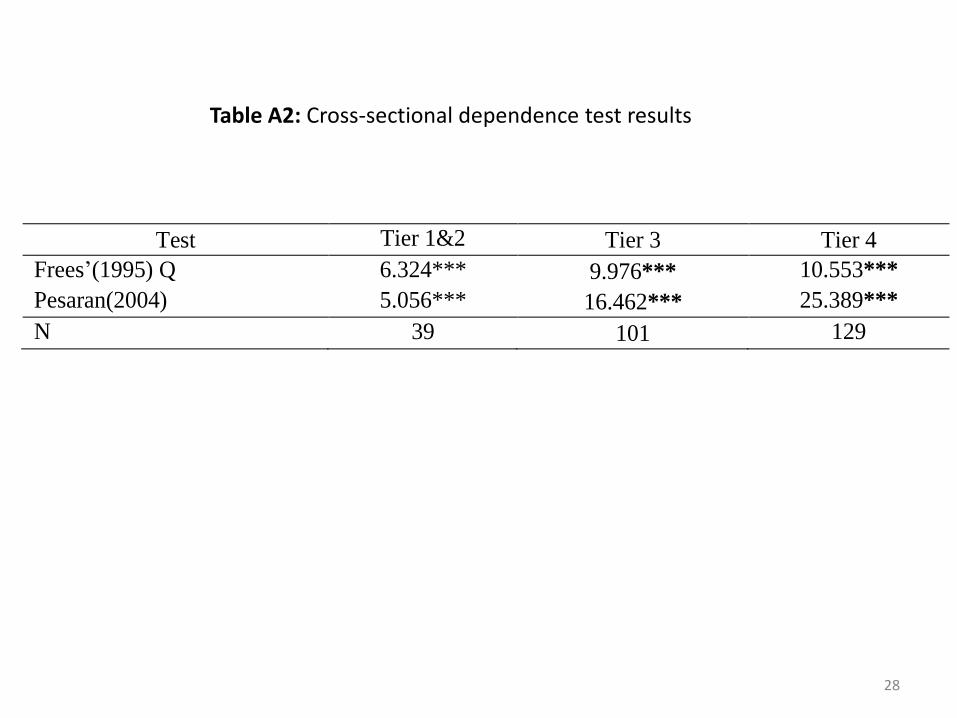
Test Tier 1&2 Tier 3 Tier 4

Frees’(1995) Q 6.324*** 9.976*** 10.553***

Pesaran(2004) 5.056*** 16.462*** 25.389***

N 39 101 129

Table A2: Cross-sectional dependence test results

28

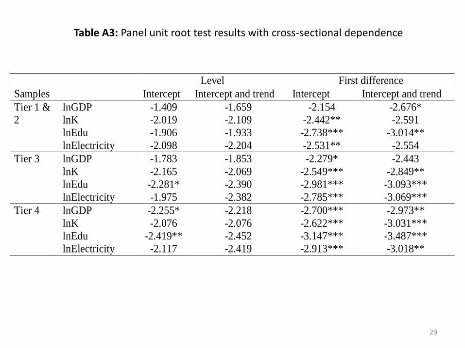
Level First difference

Samples Intercept Intercept and trend Intercept Intercept and trend

Tier 1 &

2

lnGDP -1.409 -1.659 -2.154 -2.676*

lnK -2.019 -2.109 -2.442** -2.591

lnEdu -1.906 -1.933 -2.738*** -3.014**

lnElectricity -2.098 -2.204 -2.531** -2.554

Tier 3 lnGDP -1.783 -1.853 -2.279* -2.443

lnK -2.165 -2.069 -2.549*** -2.849**

lnEdu -2.281* -2.390 -2.981*** -3.093***

lnElectricity -1.975 -2.382 -2.785*** -3.069***

Tier 4 lnGDP -2.255* -2.218 -2.700*** -2.973**

lnK -2.076 -2.076 -2.622*** -3.031***

lnEdu -2.419** -2.452 -3.147*** -3.487***

lnElectricity -2.117 -2.419 -2.913*** -3.018**

Table A3: Panel unit root test results with cross-sectional dependence

29

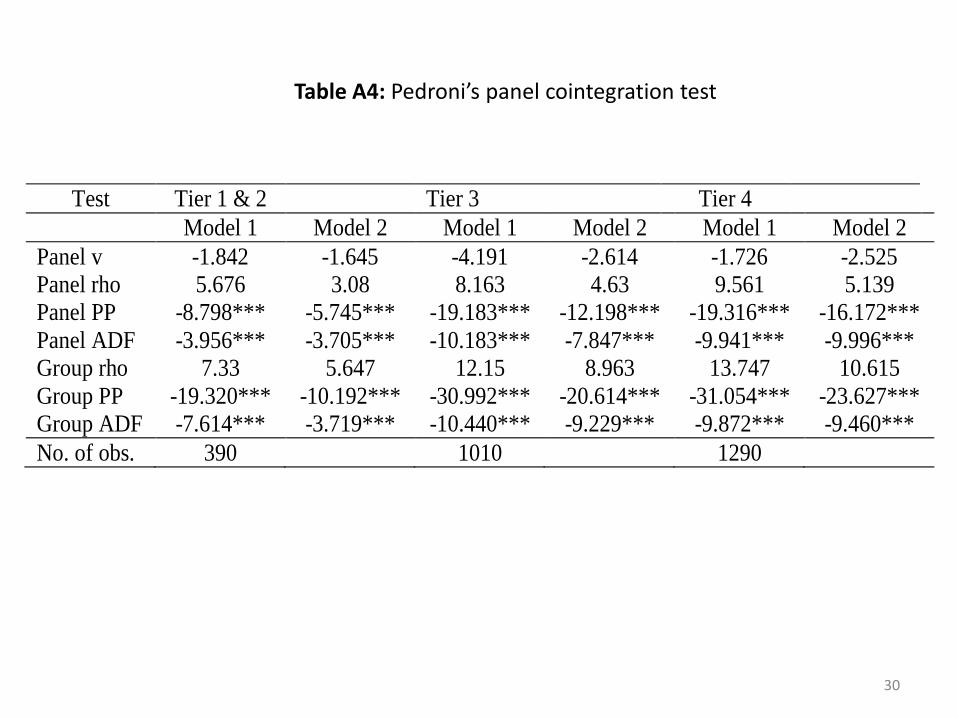
Test Tier 1 & 2 Tier 3 Tier 4

Model 1 Model 2 Model 1 Model 2 Model 1 Model 2

Panel v -1.842 -1.645 -4.191 -2.614 -1.726 -2.525

Panel rho 5.676 3.08 8.163 4.63 9.561 5.139

Panel PP -8.798*** -5.745*** -19.183*** -12.198*** -19.316*** -16.172***

Panel ADF -3.956*** -3.705*** -10.183*** -7.847*** -9.941*** -9.996***

Group rho 7.33 5.647 12.15 8.963 13.747 10.615

Group PP -19.320*** -10.192*** -30.992*** -20.614*** -31.054*** -23.627***

Group ADF -7.614*** -3.719*** -10.440*** -9.229*** -9.872*** -9.460***

No. of obs. 390 1010 1290

Table A4: Pedroni’s panel cointegration test

30

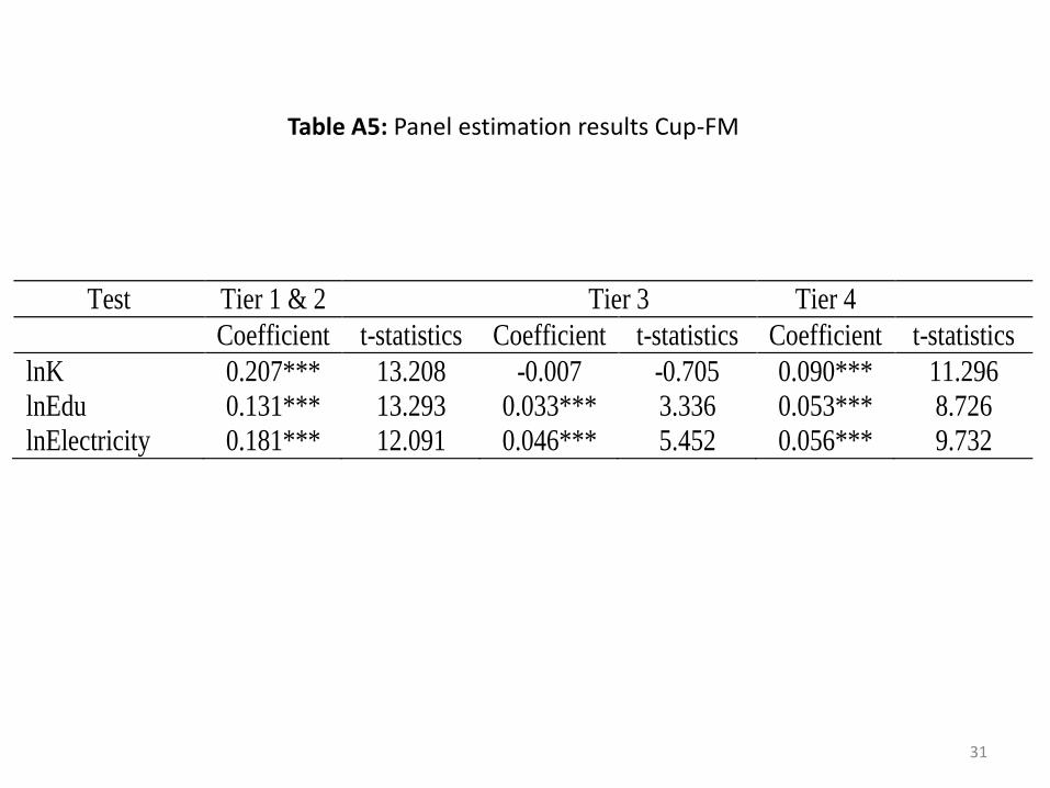
Test Tier 1 & 2 Tier 3 Tier 4

Coefficient t-statistics Coefficient t-statistics Coefficient t-statistics

lnK 0.207*** 13.208 -0.007 -0.705 0.090*** 11.296

lnEdu 0.131*** 13.293 0.033*** 3.336 0.053*** 8.726

lnElectricity 0.181*** 12.091 0.046*** 5.452 0.056*** 9.732

Table A5: Panel estimation results Cup-FM

31

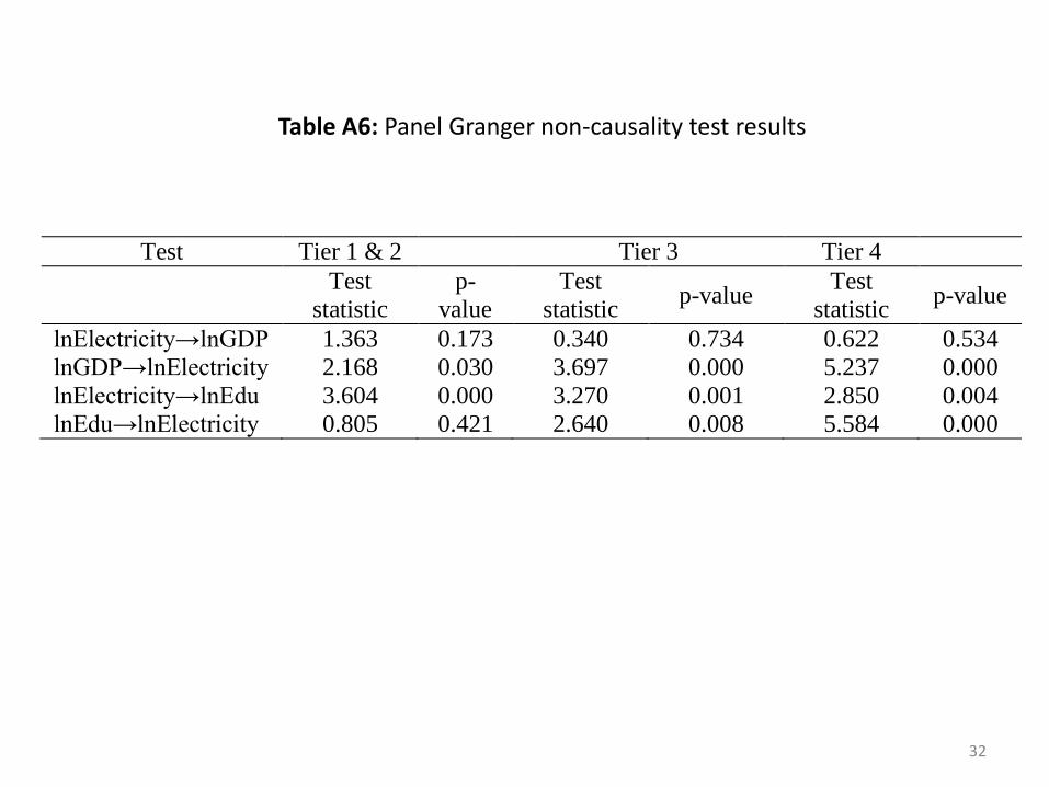
Test Tier 1 & 2 Tier 3 Tier 4

Test

statistic

p-

value

Test

statistic p-value

Test

statistic p-value

lnElectricity→lnGDP 1.363 0.173 0.340 0.734 0.622 0.534

lnGDP→lnElectricity 2.168 0.030 3.697 0.000 5.237 0.000

lnElectricity→lnEdu 3.604 0.000 3.270 0.001 2.850 0.004

lnEdu→lnElectricity 0.805 0.421 2.640 0.008 5.584 0.000

Table A6: Panel Granger non-causality test results

32

Conclusion

• For China as a whole physical and human capital have similar positive impacts as electricity consumption on local economic growth.

• Electricity consumption plays a dominant role to boost growth in the Center; human capital contributes most to growth in the East; physical capital facilitates growth in the West.

• We find a uni-directional causal relation running from economic growth to electricity consumption in central and western China and a feedback effects in eastern China.

33

Conclusion

• Electricity granger causes education expenditure in some eastern Chinese cities and a reverse relation is observed for cities in Middle China, while for western cities a bi-directional causal link is found.

• National and decentralized local policies and targets should be reexamined and coordinated across government agencies.

34