HAL Id: hal-00023493https://hal-insu.archives-ouvertes.fr/hal-00023493

Submitted on 10 May 2006

HAL is a multi-disciplinary open accessarchive for the deposit and dissemination of sci-entific research documents, whether they are pub-lished or not. The documents may come fromteaching and research institutions in France orabroad, or from public or private research centers.

L’archive ouverte pluridisciplinaire HAL, estdestinée au dépôt et à la diffusion de documentsscientifiques de niveau recherche, publiés ou non,émanant des établissements d’enseignement et derecherche français ou étrangers, des laboratoirespublics ou privés.

Electrical resistivity survey in soil science: a review .Anatja Samouëlian, Isabelle Cousin, Alain Tabbagh, Ary Bruand, Guy

Richard

To cite this version:Anatja Samouëlian, Isabelle Cousin, Alain Tabbagh, Ary Bruand, Guy Richard. Electrical resistiv-ity survey in soil science: a review .. Soil and Tillage Research, Elsevier, 2005, 83, pp.2, 173-193.<10.1016/j.still.2004.10.004>. <hal-00023493>

Electrical resistivity survey in soil science: a review A. Samouelian a,b,*, I. Cousin a, A. Tabbagh c, A. Bruand d, G. Richard e a/ INRA, Unité de Science du Sol, BP 20619, 45166 Ardon, France b/ Universitat Heidelberg, Institut fur Umweltphysik INF 229, 69120 Heidelberg, Germany c/ UMR 7619 ‘‘SISYPHE’’ Case 105, 4 Place Jussieu, 75005 Paris, France d/ ISTO, UMR 6113 CNRS-UO, Université d’Orléans, Ge´osciences, BP 6759, 45067 Orléans Cedex 2, France e/ INRA Unité d’Agromonie, rue Fernand Christ, 02007 Laon, France Abstract Electrical resistivity of the soil can be considered as a proxy for the spatial and temporal variability of many other soil physical properties (i.e. structure, water content, or fluid composition). Because the method is non-destructive and very sensitive, it offers a very attractive tool for describing the subsurface properties without digging. It has been already applied in various contexts like : groundwater exploration, landfill and solute transfer delineation, agronomical management by identifying areas of excessive compaction or soil horizon thickness and bedrock depth, and at least assessing the soil hydrological properties. The surveys, depending on the areas heterogeneities can be performed in one-, two- or three-dimensions and also at different scales resolution from the centimetric scale to the regional scale. In this review, based on many electrical resistivity surveys, we expose the theory and the basic principles of the method, we overview the variation of electrical resistivity as a function of soil properties, we listed the main electrical device to performed one-, two- or three-dimensional surveys, and explain the basic principles of the data interpretation. At least, we discuss the main advantages and limits of the method. 1. Introduction The changes caused on soil by intensive agricultural production are variable in space and time. As a consequence, a continuous and precise spatially and temporal follow-up of the soil physical and chemical properties is required. Geophysical methods have been applied to soil sciences for a considerable period. The general principle of geophysical exploration is to non intrusively collect data on the medium under investigation (Scollar et al., 1990). Among such methods, those based on the electric properties seem particularly promising because soil materials and properties are strongly correlated and can be quantified through the geoelectrical properties. Indeed, the flux of electrical charges through materials permits conductor materials like metal or electrolytes, where the conductivity is great, to be distinguished from insulating materials like air, ice and plastics, where it is small. Among the latter, soil materials exhibit intermediate electrical properties depending on their physical and chemical properties (texture, salinity or water content). Schlumberger in 1912 cited by Meyer de Stadelhofen (1991) introduced the idea of using electrical resistivity measurements to study subsurface rock bodies. This method was first adopted in geology by oil companies searching for petroleum reservoirs and delineating geological formations. In soil science, Bevan (2000) reported that the first known equipotential map was compiled by Malamphy in 1938 for archaeological research at the site of Williamsburg in USA. Since that early study, the interest in subsurface soil prospecting by electrical prospecting has steadily increased. In this paper, we review the literature dealing with the use of electrical resistivity applied to soil. We first present the basic concept of the method and the different array devices. Then, we discuss the sensitivity of the electrical measurements to the soil

properties. Finally, the advantages and limitations of electrical resistivity in soil survey and the application to agricultural management are discussed. 2. Theory and basic principles The purpose of electrical resistivity surveys is to determine the resistivity distribution of the sounding soil volume. Artificially generated electric currents are supplied to the soil and the resulting potential differences are measured. Potential difference patterns provide information on the form of subsurface heterogeneities and of their electrical properties (Kearey et al., 2002). The greater the electrical contrast between the soil matrix and heterogeneity, the easier is the detection. Electrical resistivity of the soil can be considered as a proxy for the variability of soil physical properties (Banton et al., 1997). The current flow line distributions depend on the medium under investigation; they are concentrated in conductive volumes. For a simple body, the resistivity r (Ω m) is defined as follows :

with R being the electrical resistance (Ω), L the length of the cylinder (m) and S is its cross-sectional area (m2). The electrical resistance of the cylindrical body R (Ω), is defined by the Ohm’s law as follows:

with V being the potential (V) and I is the current (A). Electrical characteristic is also commonly described by the conductivity value σ (Sm_1), equal to the reciprocal of the soil resistivity. Thus :

In a homogeneous and isotropic half-space, electrical equipotentials are hemispherical when the current electrodes are located at the soil surface as shown in Fig. 1 (Scollar et al., 1990; Kearey et al., 2002; Sharma, 1997; Reynolds, 1997). The current density J (A/m2) has then to be calculated for all the radial directions with :

where 2πr2 is the surface of a hemispherical sphere of radius r. The potential V can then be expressed as follows:

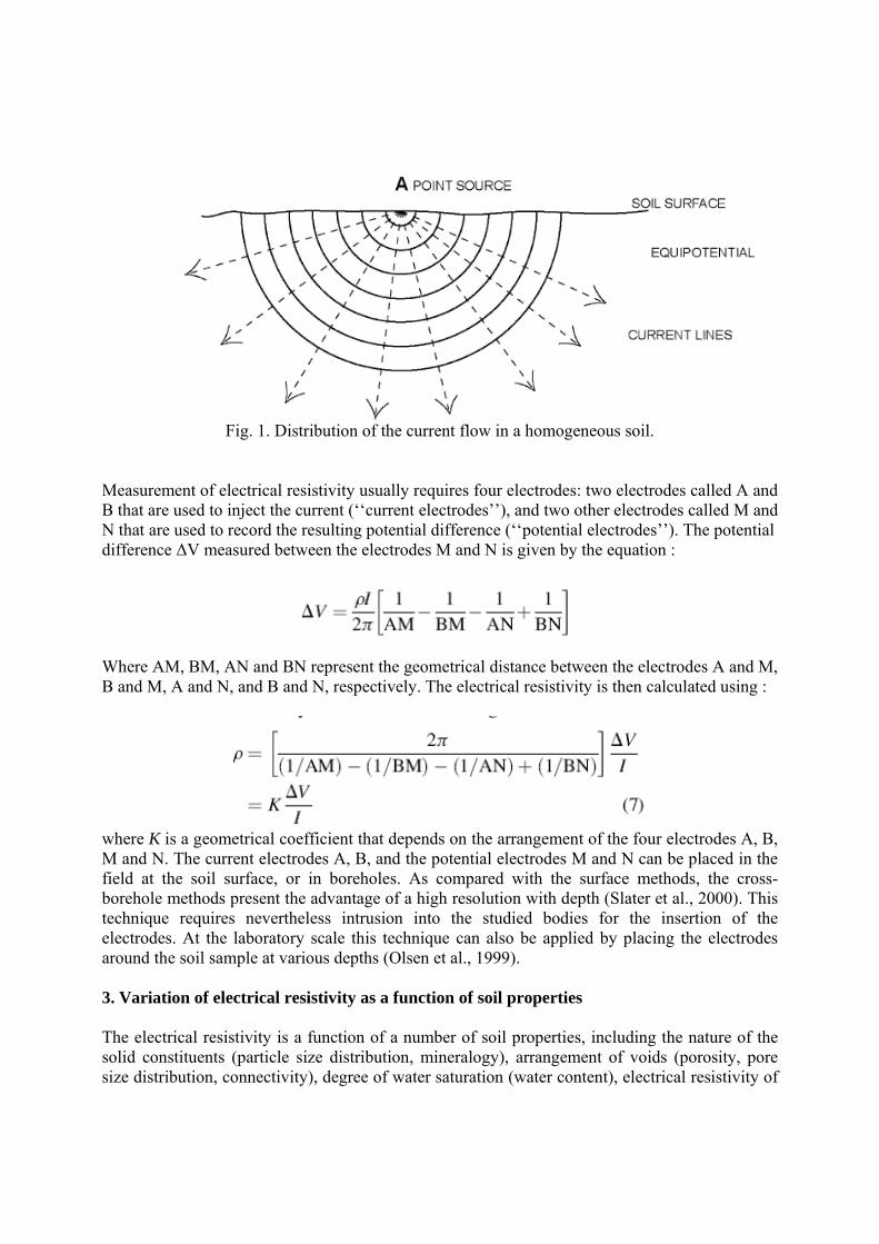
Fig. 1. Distribution of the current flow in a homogeneous soil.

Measurement of electrical resistivity usually requires four electrodes: two electrodes called A and B that are used to inject the current (‘‘current electrodes’’), and two other electrodes called M and N that are used to record the resulting potential difference (‘‘potential electrodes’’). The potential difference ΔV measured between the electrodes M and N is given by the equation :

Where AM, BM, AN and BN represent the geometrical distance between the electrodes A and M, B and M, A and N, and B and N, respectively. The electrical resistivity is then calculated using :

where K is a geometrical coefficient that depends on the arrangement of the four electrodes A, B, M and N. The current electrodes A, B, and the potential electrodes M and N can be placed in the field at the soil surface, or in boreholes. As compared with the surface methods, the cross-borehole methods present the advantage of a high resolution with depth (Slater et al., 2000). This technique requires nevertheless intrusion into the studied bodies for the insertion of the electrodes. At the laboratory scale this technique can also be applied by placing the electrodes around the soil sample at various depths (Olsen et al., 1999). 3. Variation of electrical resistivity as a function of soil properties The electrical resistivity is a function of a number of soil properties, including the nature of the solid constituents (particle size distribution, mineralogy), arrangement of voids (porosity, pore size distribution, connectivity), degree of water saturation (water content), electrical resistivity of

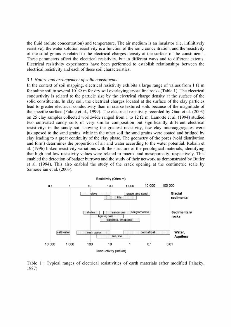
the fluid (solute concentration) and temperature. The air medium is an insulator (i.e. infinitively resistive), the water solution resistivity is a function of the ionic concentration, and the resistivity of the solid grains is related to the electrical charges density at the surface of the constituents. These parameters affect the electrical resistivity, but in different ways and to different extents. Electrical resistivity experiments have been performed to establish relationships between the electrical resistivity and each of these soil characteristics. 3.1. Nature and arrangement of solid constituents In the context of soil mapping, electrical resistivity exhibits a large range of values from 1 Ω m for saline soil to several 105 Ω m for dry soil overlaying crystalline rocks (Table 1). The electrical conductivity is related to the particle size by the electrical charge density at the surface of the solid constituents. In clay soil, the electrical charges located at the surface of the clay particles lead to greater electrical conductivity than in coarse-textured soils because of the magnitude of the specific surface (Fukue et al., 1999). The electrical resistivity recorded by Giao et al. (2003) on 25 clay samples collected worldwide ranged from 1 to 12 Ω m. Lamotte et al. (1994) studied two cultivated sandy soils of very similar composition but significantly different electrical resistivity: in the sandy soil showing the greatest resistivity, few clay microaggregates were juxtaposed to the sand grains, while in the other soil the sand grains were coated and bridged by clay leading to a great continuity of the clay phase. The geometry of the pores (void distribution and form) determines the proportion of air and water according to the water potential. Robain et al. (1996) linked resistivity variations with the structure of the pedological materials, identifying that high and low resistivity values were related to macro- and mesoporosity, respectively. This enabled the detection of badger burrows and the study of their network as demonstrated by Butler et al. (1994). This also enabled the study of the crack opening at the centimetric scale by Samouelian et al. (2003).

Table 1 : Typical ranges of electrical resistivities of earth materials (after modified Palacky, 1987)

The porosity can be obtained for the electrical property via the Archie’s law, which for a saturated soil without clay is written as :

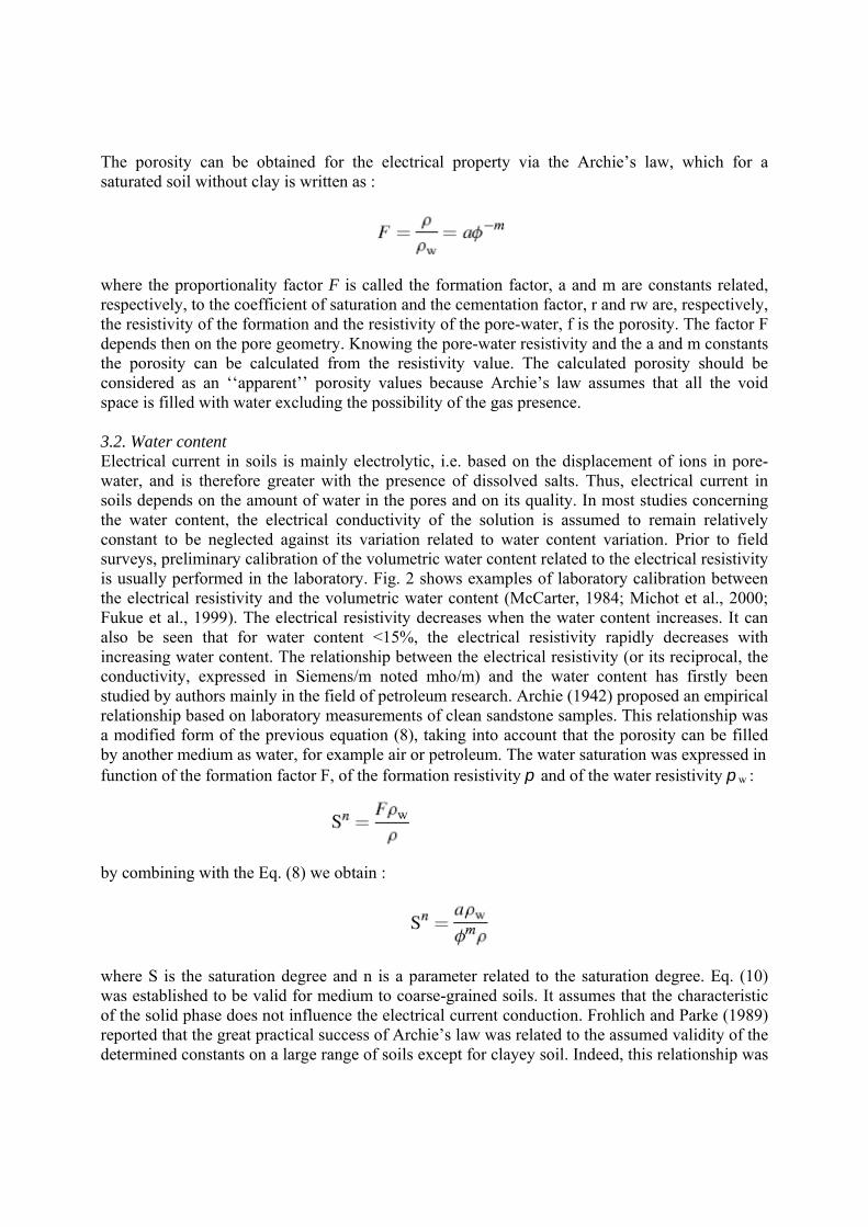
where the proportionality factor F is called the formation factor, a and m are constants related, respectively, to the coefficient of saturation and the cementation factor, r and rw are, respectively, the resistivity of the formation and the resistivity of the pore-water, f is the porosity. The factor F depends then on the pore geometry. Knowing the pore-water resistivity and the a and m constants the porosity can be calculated from the resistivity value. The calculated porosity should be considered as an ‘‘apparent’’ porosity values because Archie’s law assumes that all the void space is filled with water excluding the possibility of the gas presence. 3.2. Water content Electrical current in soils is mainly electrolytic, i.e. based on the displacement of ions in pore-water, and is therefore greater with the presence of dissolved salts. Thus, electrical current in soils depends on the amount of water in the pores and on its quality. In most studies concerning the water content, the electrical conductivity of the solution is assumed to remain relatively constant to be neglected against its variation related to water content variation. Prior to field surveys, preliminary calibration of the volumetric water content related to the electrical resistivity is usually performed in the laboratory. Fig. 2 shows examples of laboratory calibration between the electrical resistivity and the volumetric water content (McCarter, 1984; Michot et al., 2000; Fukue et al., 1999). The electrical resistivity decreases when the water content increases. It can also be seen that for water content <15%, the electrical resistivity rapidly decreases with increasing water content. The relationship between the electrical resistivity (or its reciprocal, the conductivity, expressed in Siemens/m noted mho/m) and the water content has firstly been studied by authors mainly in the field of petroleum research. Archie (1942) proposed an empirical relationship based on laboratory measurements of clean sandstone samples. This relationship was a modified form of the previous equation (8), taking into account that the porosity can be filled by another medium as water, for example air or petroleum. The water saturation was expressed in function of the formation factor F, of the formation resistivity p and of the water resistivity pw :

by combining with the Eq. (8) we obtain :

where S is the saturation degree and n is a parameter related to the saturation degree. Eq. (10) was established to be valid for medium to coarse-grained soils. It assumes that the characteristic of the solid phase does not influence the electrical current conduction. Frohlich and Parke (1989) reported that the great practical success of Archie’s law was related to the assumed validity of the determined constants on a large range of soils except for clayey soil. Indeed, this relationship was

successfully used for water content estimation in numerous studies (Binley et al., 2002; Zhou et al., 2001). An empirical linear relationship between the resistivity and the water content was proposed by Goyal et al. (1996) and Gupta and Hanks (1972) as follows :

where a and b are empirical constants implicitly containing the soil and water characteristics (i.e. porosity, temperature, salinity) and assumed to be invariant with time. Temporal variations in the soil moisture profile are estimated by using electrical resistivity sounding data acquired at different times (Aaltonen, 2001; Michot et al., 2003).

Fig. 2. Relationship between the volumetric water content and the electrical resistivity for different soil types (values issues from Fukue et al., 1999; Michot et al., 2003; McCarter, 1984).

where ps and pw represent the solid matrix and the pore-water resistivity, respectively, a and b are coefficients depending on the solid phase characteristics, related to the texture and mineralogy, and u is the volumetric water content (cm3 cm-3). By using Eq. (12), Kalinski and Kelly (1993) predicted the volumetric water content with a standard error of 0.009 for water contents ranging from 0.20 to 0.50 in soil containing 20% clay.

3.3. Pore fluid composition As outlined above, the electrical conductivity is related to the mobility of the ions present in the fluid filling the pores. Conductivity depends on the concentration and the viscosity of the water (Scollar et al., 1990). The estimation of the water content by resistivity measurements requires a knowledge of the concentration of dissolved ions. Early studies dealing with the determination of the soil water content were confronted with the problem of estimating the soil salinity variation (Rhoades et al., 1977). Since salts have to be in an ionized form to conduct the current, the amount of water in soil governs the available paths of conduction. Shea and Luthin (1961) found a close linear relationship between electrical resistivity and salinity for a soil water content ranging from saturation to -3 kPa water potential. Thus, estimation of the soil salinity by electrical resistivity requires measurements made at the same water content. The soil salinity is usually measured at saturation, as this is considered as a standardized condition. Kalinski and Kelly (1993) estimated the volumetric water content using Eq. (12) and with pore solution resistivity (pw) of 1, 2 and 3 mmho/cm. They found that at a given water content, the electrical resistivity decreases when the water conductivity increases (Fig. 3). Moreover, the different ions present in the solution (H+, OH-, SO4

2-, Na+, Cl-, . . .) do not affect the conductivity in the same way because of differences in ion mobility. This explains why soil solutions at the same concentration but having different ionic compositions, may have different electrical conductivities. This results in a large range of possible electrical conductivities because of concentration and ionic composition variations in different areas of the soil. This property was also used by Bernstone et al. (1998) to delineate landfill structure. The large resistivity contrast between salt water- and fresh water-saturated zones was used by several investigators to study salt water intrusion into coastal areas (Nowroozi et al., 1999; Acworth, 1999; Yaramanci, 2000). Van Dam and Meulenkamp (1967) considered the soil resistivity values of 40, 12 and 3 Ω m as representative of fresh, brackish and saline water, respectively. 3.4. Temperature Ion agitation increases with temperature when the viscosity of a fluid decreases. Thus, the electrical resistivity decreases when the temperature increases. Comparisons of electrical resistivity measurements require the expression of the electrical resistivity at a standardized temperature. By conducting laboratory experiments on 30 samples of saline and alkaline soils, Campbell et al. (1948) showed that conductivity increased by 2.02% per °C between 15 and 35 °C.

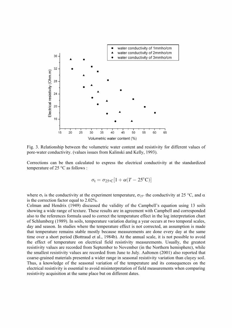
Fig. 3. Relationship between the volumetric water content and resistivity for different values of pore-water conductivity. (values issues from Kalinski and Kelly, 1993). Corrections can be then calculated to express the electrical conductivity at the standardized temperature of 25 °C as follows :

where σt is the conductivity at the experiment temperature, σ25° the conductivity at 25 °C, and α is the correction factor equal to 2.02%. Colman and Hendrix (1949) discussed the validity of the Campbell’s equation using 13 soils showing a wide range of texture. These results are in agreement with Campbell and corresponded also to the references formula used to correct the temperature effect in the log interpretation chart of Schlumberg (1989). In soils, temperature variation during a year occurs at two temporal scales, day and season. In studies where the temperature effect is not corrected, an assumption is made that temperature remains stable mostly because measurements are done every day at the same time over a short period (Bottraud et al., 1984b). At the annual scale, it is not possible to avoid the effect of temperature on electrical field resistivity measurements. Usually, the greatest resistivity values are recorded from September to November (in the Northern hemisphere), while the smallest resistivity values are recorded from June to July. Aaltonen (2001) also reported that coarse-grained materials presented a wider range in seasonal resistivity variation than clayey soil. Thus, a knowledge of the seasonal variation of the temperature and its consequences on the electrical resistivity is essential to avoid misinterpretation of field measurements when comparing resistivity acquisition at the same place but on different dates.

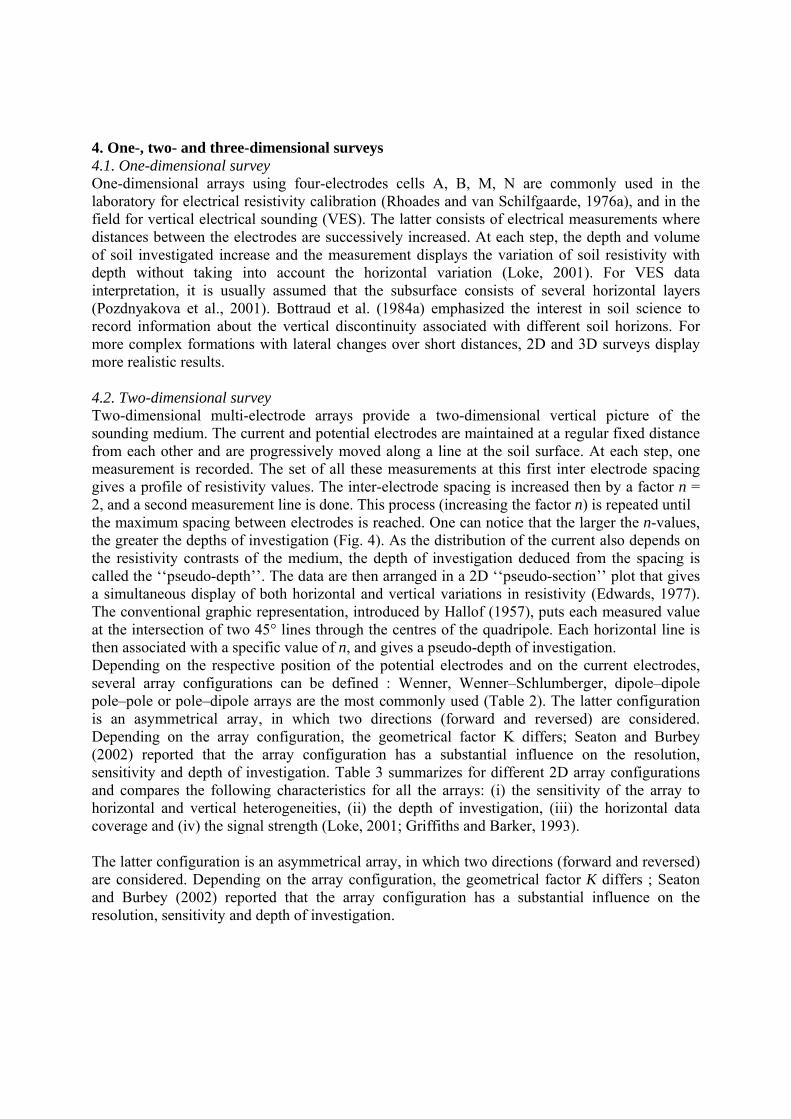
4. One-, two- and three-dimensional surveys 4.1. One-dimensional survey One-dimensional arrays using four-electrodes cells A, B, M, N are commonly used in the laboratory for electrical resistivity calibration (Rhoades and van Schilfgaarde, 1976a), and in the field for vertical electrical sounding (VES). The latter consists of electrical measurements where distances between the electrodes are successively increased. At each step, the depth and volume of soil investigated increase and the measurement displays the variation of soil resistivity with depth without taking into account the horizontal variation (Loke, 2001). For VES data interpretation, it is usually assumed that the subsurface consists of several horizontal layers (Pozdnyakova et al., 2001). Bottraud et al. (1984a) emphasized the interest in soil science to record information about the vertical discontinuity associated with different soil horizons. For more complex formations with lateral changes over short distances, 2D and 3D surveys display more realistic results. 4.2. Two-dimensional survey Two-dimensional multi-electrode arrays provide a two-dimensional vertical picture of the sounding medium. The current and potential electrodes are maintained at a regular fixed distance from each other and are progressively moved along a line at the soil surface. At each step, one measurement is recorded. The set of all these measurements at this first inter electrode spacing gives a profile of resistivity values. The inter-electrode spacing is increased then by a factor n = 2, and a second measurement line is done. This process (increasing the factor n) is repeated until the maximum spacing between electrodes is reached. One can notice that the larger the n-values, the greater the depths of investigation (Fig. 4). As the distribution of the current also depends on the resistivity contrasts of the medium, the depth of investigation deduced from the spacing is called the ‘‘pseudo-depth’’. The data are then arranged in a 2D ‘‘pseudo-section’’ plot that gives a simultaneous display of both horizontal and vertical variations in resistivity (Edwards, 1977). The conventional graphic representation, introduced by Hallof (1957), puts each measured value at the intersection of two 45° lines through the centres of the quadripole. Each horizontal line is then associated with a specific value of n, and gives a pseudo-depth of investigation. Depending on the respective position of the potential electrodes and on the current electrodes, several array configurations can be defined : Wenner, Wenner–Schlumberger, dipole–dipole pole–pole or pole–dipole arrays are the most commonly used (Table 2). The latter configuration is an asymmetrical array, in which two directions (forward and reversed) are considered. Depending on the array configuration, the geometrical factor K differs; Seaton and Burbey (2002) reported that the array configuration has a substantial influence on the resolution, sensitivity and depth of investigation. Table 3 summarizes for different 2D array configurations and compares the following characteristics for all the arrays: (i) the sensitivity of the array to horizontal and vertical heterogeneities, (ii) the depth of investigation, (iii) the horizontal data coverage and (iv) the signal strength (Loke, 2001; Griffiths and Barker, 1993). The latter configuration is an asymmetrical array, in which two directions (forward and reversed) are considered. Depending on the array configuration, the geometrical factor K differs ; Seaton and Burbey (2002) reported that the array configuration has a substantial influence on the resolution, sensitivity and depth of investigation.

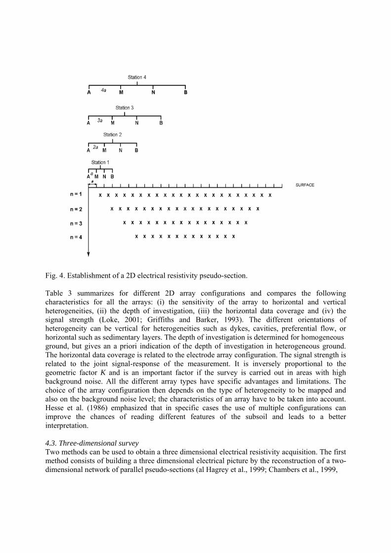
Fig. 4. Establishment of a 2D electrical resistivity pseudo-section. Table 3 summarizes for different 2D array configurations and compares the following characteristics for all the arrays: (i) the sensitivity of the array to horizontal and vertical heterogeneities, (ii) the depth of investigation, (iii) the horizontal data coverage and (iv) the signal strength (Loke, 2001; Griffiths and Barker, 1993). The different orientations of heterogeneity can be vertical for heterogeneities such as dykes, cavities, preferential flow, or horizontal such as sedimentary layers. The depth of investigation is determined for homogeneous ground, but gives an a priori indication of the depth of investigation in heterogeneous ground. The horizontal data coverage is related to the electrode array configuration. The signal strength is related to the joint signal-response of the measurement. It is inversely proportional to the geometric factor K and is an important factor if the survey is carried out in areas with high background noise. All the different array types have specific advantages and limitations. The choice of the array configuration then depends on the type of heterogeneity to be mapped and also on the background noise level; the characteristics of an array have to be taken into account. Hesse et al. (1986) emphasized that in specific cases the use of multiple configurations can improve the chances of reading different features of the subsoil and leads to a better interpretation. 4.3. Three-dimensional survey Two methods can be used to obtain a three dimensional electrical resistivity acquisition. The first method consists of building a three dimensional electrical picture by the reconstruction of a two-dimensional network of parallel pseudo-sections (al Hagrey et al., 1999; Chambers et al., 1999,

2002; Oglivy et al., 1999; Zhou et al., 2001). An accurate three-dimensional electrical picture is thus recorded if electrical anomalies are preferentially oriented and if the in-line measurement electrodes are perpendicular to the orientation of the anomalies. Chambers et al. (2002) outlined that electrical surveys using co-linear arrays carried out on sites with heterogeneous subsurface conditions should include measurements using electrode configurations oriented in at least two directions perpendicular to one another. Zhou et al. (2001) mapped 3D electrical resistivity with several 2D parallel pseudo-sections along the X, Y, XY and -XY directions, enabling the study of an anisotropic media. The second method consists of using a square array of four electrodes (Table 2). Habberjam and Watkins (1967) showed that such an array provides a measure of resistivity less orientation-dependent than that given by an in-line array. Senos Matias (2002) emphasizes too that the data were orientationally stable, so there was no need for prior knowledge of the electrical heterogeneity orientation. He recommended then to use this array over anisotropic ground.

Table 2 Example of 2D in-line electrodes array configuration, and 3D electrode device

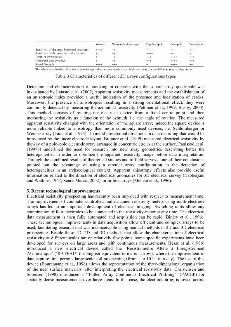
Table 3 Characteristics of different 2D arrays configurations types

Detection and characterisation of cracking in concrete with the square array quadripole was investigated by Lataste et al. (2002).Apparent resistivity measurements and the establishment of an anisotropic index provided a useful indication of the presence and localization of cracks. Moreover, the presence of anisotropies resulting in a strong orientational effect, they were commonly detected by measuring the azimuthal resistivity (Pettinen et al., 1999; Busby, 2000). This method consists of rotating the electrical device from a fixed centre point and then measuring the resistivity as a function of the azimuth, i.e. the angle of rotation. The measured apparent resistivity changed with the orientation of the square array; indeed the square device is more reliable linked to anisotropy than more commonly used devices, i.e. Schlumberger or Wenner array (Lane et al., 1995). To avoid preferential directions in data recording that would be introduced by the linear electrode layout, Brunner et al. (1999) measured electrical resistivity by theway of a pole–pole electrode array arranged in concentric circles at the surface. Panissod et al. (1997b) underlined the need for research into new array geometries describing better the heterogeneities in order to optimize the apparent resistivity image before data interpretation. Through the combined results of theoretical studies and of field surveys, one of their conclusions pointed out the advantage of using a circular array configuration in the detection of heterogeneities in an archaeological context. Apparent anisotropy effects also provide useful information related to the direction of electrical anomalies for 3D electrical survey (Habberjam and Watkins, 1967; Senos Matias, 2002), or in-line arrays (Meheni et al., 1996). 5. Recent technological improvements Electrical resistivity prospecting has recently been improved with respect to measurement time. The improvement of computer-controlled multi-channel resistivity-meters using multi-electrode arrays has led to an important development of electrical imaging. Switching units allow any combination of four electrodes to be connected to the resistivity-meter at any time. The electrical data measurement is then fully automated and acquisition can be rapid (Binley et al., 1996). These technological improvements in data acquisition allow efficient and complex arrays to be used, facilitating research that was inconceivable using manual methods in 2D and 3D electrical prospecting. Beside these 1D, 2D and 3D methods that allow the characterisation of electrical resistivity at different scales but on relatively few points, some specific experiments have been developed for surveys on large areas and with continuous measurements. Hesse et al. (1986) introduced a new electrical device called the ‘Résistivimètre Attelé à Enregistrement AUtomatique’ (‘RATEAU’ the English equivalent terms is harrow), where the improvement in data capture time permits large scale soil prospecting (from 1 to 10 ha in a day). The use of this device (Bourennane et al., 1998) allows the representation of the three-dimensional organisation of the near surface materials, after interpreting the electrical resistivity data. Christensen and Sorensen (1998) introduced a ‘‘Pulled Array Continuous Electrical Profiling’’ (PACEP) for spatially dense measurements over large areas. In this case, the electrode array is towed across

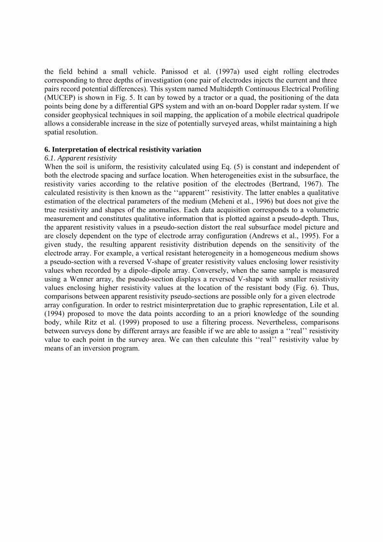
the field behind a small vehicle. Panissod et al. (1997a) used eight rolling electrodes corresponding to three depths of investigation (one pair of electrodes injects the current and three pairs record potential differences). This system named Multidepth Continuous Electrical Profiling (MUCEP) is shown in Fig. 5. It can by towed by a tractor or a quad, the positioning of the data points being done by a differential GPS system and with an on-board Doppler radar system. If we consider geophysical techniques in soil mapping, the application of a mobile electrical quadripole allows a considerable increase in the size of potentially surveyed areas, whilst maintaining a high spatial resolution. 6. Interpretation of electrical resistivity variation 6.1. Apparent resistivity When the soil is uniform, the resistivity calculated using Eq. (5) is constant and independent of both the electrode spacing and surface location. When heterogeneities exist in the subsurface, the resistivity varies according to the relative position of the electrodes (Bertrand, 1967). The calculated resistivity is then known as the ‘‘apparent’’ resistivity. The latter enables a qualitative estimation of the electrical parameters of the medium (Meheni et al., 1996) but does not give the true resistivity and shapes of the anomalies. Each data acquisition corresponds to a volumetric measurement and constitutes qualitative information that is plotted against a pseudo-depth. Thus, the apparent resistivity values in a pseudo-section distort the real subsurface model picture and are closely dependent on the type of electrode array configuration (Andrews et al., 1995). For a given study, the resulting apparent resistivity distribution depends on the sensitivity of the electrode array. For example, a vertical resistant heterogeneity in a homogeneous medium shows a pseudo-section with a reversed V-shape of greater resistivity values enclosing lower resistivity values when recorded by a dipole–dipole array. Conversely, when the same sample is measured using a Wenner array, the pseudo-section displays a reversed V-shape with smaller resistivity values enclosing higher resistivity values at the location of the resistant body (Fig. 6). Thus, comparisons between apparent resistivity pseudo-sections are possible only for a given electrode array configuration. In order to restrict misinterpretation due to graphic representation, Lile et al. (1994) proposed to move the data points according to an a priori knowledge of the sounding body, while Ritz et al. (1999) proposed to use a filtering process. Nevertheless, comparisons between surveys done by different arrays are feasible if we are able to assign a ‘‘real’’ resistivity value to each point in the survey area. We can then calculate this ‘‘real’’ resistivity value by means of an inversion program.

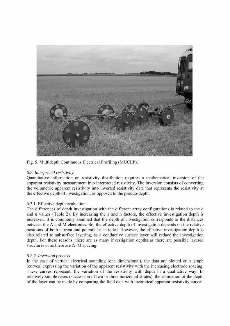
Fig. 5. Multidepth Continuous Electrical Profiling (MUCEP). 6.2. Interpreted resistivity Quantitative information on resistivity distribution requires a mathematical inversion of the apparent resistivity measurement into interpreted resistivity. The inversion consists of converting the volumetric apparent resistivity into inverted resistivity data that represents the resistivity at the effective depth of investigation, as opposed to the pseudo-depth. 6.2.1. Effective depth evaluation The differences of depth investigation with the different array configurations is related to the a and n values (Table 2). By increasing the a and n factors, the effective investigation depth is increased. It is commonly assumed that the depth of investigation corresponds to the distances between the A and M electrodes. So, the effective depth of investigation depends on the relative positions of both current and potential electrodes. However, the effective investigation depth is also related to subsurface layering, as a conductive surface layer will reduce the investigation depth. For these reasons, there are as many investigation depths as there are possible layered structures or as there are A–M spacing. 6.2.2. Inversion process In the case of vertical electrical sounding (one dimensional), the data are plotted on a graph (curves) expressing the variation of the apparent resistivity with the increasing electrode spacing. These curves represent, the variation of the resistivity with depth in a qualitative way. In relatively simple cases (succession of two or three horizontal strates), the estimation of the depth of the layer can be made by comparing the field data with theoretical apparent resistivity curves.

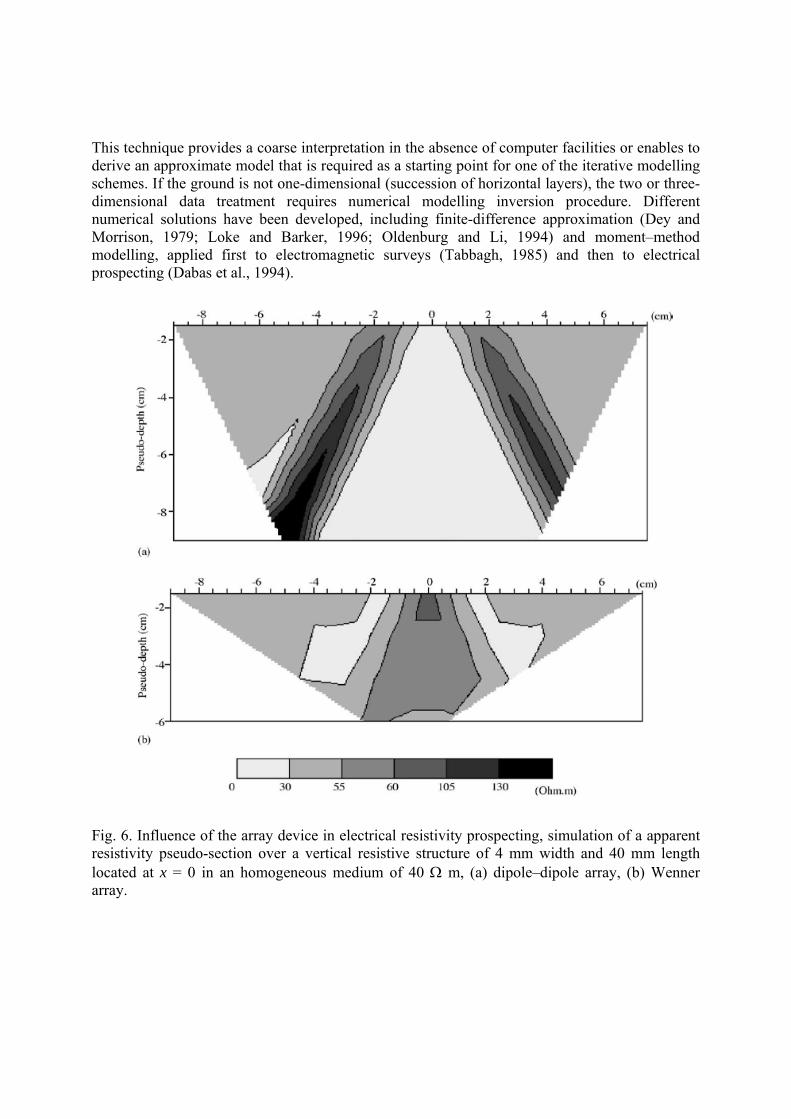
This technique provides a coarse interpretation in the absence of computer facilities or enables to derive an approximate model that is required as a starting point for one of the iterative modelling schemes. If the ground is not one-dimensional (succession of horizontal layers), the two or three-dimensional data treatment requires numerical modelling inversion procedure. Different numerical solutions have been developed, including finite-difference approximation (Dey and Morrison, 1979; Loke and Barker, 1996; Oldenburg and Li, 1994) and moment–method modelling, applied first to electromagnetic surveys (Tabbagh, 1985) and then to electrical prospecting (Dabas et al., 1994).

Fig. 6. Influence of the array device in electrical resistivity prospecting, simulation of a apparent resistivity pseudo-section over a vertical resistive structure of 4 mm width and 40 mm length located at x = 0 in an homogeneous medium of 40 Ω m, (a) dipole–dipole array, (b) Wenner array.

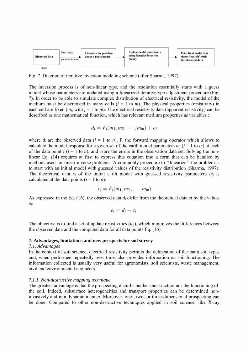
Fig. 7. Diagram of iterative inversion modeling scheme (after Sharma, 1997). The inversion process is of non-linear type, and the resolution essentially starts with a guess model whose parameters are updated using a linearized iterativetype adjustment procedure (Fig. 7). In order to be able to simulate complex distribution of electrical resistivity, the model of the medium must be discretized in many cells (j = 1 to m). The physical properties (resistivity) in each cell are fixed (mj, with j = 1 to m). The electrical resistivity data (apparent resistivity) can be described as one mathematical function, which has relevant medium properties as variables :

where di are the observed data (i = 1 to n), Fi the forward mapping operator which allows to calculate the model response for a given set of the earth model parameters mj (j = 1 to m) at each of the data point I (i = 1 to n), and ei are the errors in the observation data set. Solving the non-linear Eq. (14) requires at first to express this equation into a form that can be handled by methods used for linear inverse problems. A commonly procedure to ‘‘linearize’’ the problem is to start with an initial model with guessed values of the resistivity distribution (Sharma, 1997). The theoretical data ci of the initial earth model with guessed resistivity parameters mj is calculated at the data points (i = 1 to n).

As expressed in the Eq. (16), the observed data di differ from the theoretical data ci by the values ei:

The objective is to find a set of update resistivities (mj), which minimizes the differences between the observed data and the computed data for all data points Eq. (16). 7. Advantages, limitations and new prospects for soil survey 7.1. Advantages In the context of soil science, electrical resistivity permits the delineation of the main soil types and, when performed repeatedly over time, also provides information on soil functioning. The information collected is usually very useful for agronomists, soil scientists, waste management, civil and environmental engineers. 7.1.1. Non-destructive mapping technique The greatest advantage is that the prospecting disturbs neither the structure nor the functioning of the soil. Indeed, subsurface heterogeneities and transport properties can be determined non-invasively and in a dynamic manner. Moreover, one-, two- or three-dimensional prospecting can be done. Compared to other non-destructive techniques applied in soil science, like X-ray

tomography, Olsen et al. (1999) emphasized the possibility and advantage of monitoring resistivity variation both over long time and at decimetric scale. It can also be rapidly and easily carried out over several meters and thus applied to describe both horizontal and vertical variability of soil structure and properties at the scale of interest (Tabbagh et al., 2000). Park (1998) underlined that this method may show details of fluid migration that are unavailable with conventional hydrological monitoring technique. Preferred pathways corresponding to horizontal and vertical heterogeneities were also detected by this method and localised in the unsaturated soil zone (al Hagrey et al., 1999). 7.1.2. Temporal monitoring This approach is very appealing for monitoring the temporal changes in soil water distribution. For instance, it permits the monitoring and resolving of relatively complex flow and transport mechanism. (Slater et al., 2002). Jackson et al. (2002) identified anomalies in a roadside embankment following repeated measurement of resistivity over an 18 months period, incorporating several wet and dry seasons. Even with resistivity data, temporal monitoring can be carried out. In temporal surveys, resistivity anomalies (Drt) are computed by the Eq. (17) :

where p0, pt are resistivities at the initial stage (0) and during the temporal monitoring (t), respectively. This index is easily calculated and provides useful information on temporal variations of electrical resistivity. The differences between successive resistivity measurements are more accurate than the absolute values of these measurements, because systematic errors are eliminated. Bottraud et al. (1984a,b) observed different patterns of water distribution related to variations in grape vine growth in a homogeneous sandy soil : they established a qualitative description of water transfer using the relative variation of apparent resistivity, during monitoring periods of 2.5 months. Samouelian et al. (2003) monitored artificial cracks as they deepened and observed an increasing apparent resistivity anomaly over time. This pattern is related to climatological variation affecting the ground watertable, precipitation, and temperature. In a 2 year long experiment, Binley et al. (2002) found a clear correlation between the net rainfall and the change of the electrical resistivity in the 0–0.82 m depth. 7.1.3. Various scales application Electrical resistivity prospecting offers several advantages compared to other traditional soil prospecting (e.g. augering and excavation) and hydrological measurements (e.g. neutron probe, TDR, and tensiometry device). Classical techniques have restricted measurement scales that are usually incompatible with the subsurface variability. Electrical prospecting can be applied within a large range of scales by adjusting the inter-electrode spacing. Several different inter-electrode spacing could be applied at the same site. From the macroscopic to field scale, the measurements can be done without limitation and provide useful information. In this way, there is greater flexibility in the volume of soil that may be investigated. Jones (1995) selected this method for detecting the scaling properties of a fracture system at different resolutions (i.e. inter-electrode spacing), from 20 cm to 16 m. Depountis et al. (2001) reported a scale modelling experiment of a plume tracer by miniaturising the electrical device on a soil sample with dimensions of 75 cm x 22 cm x 12 cm, at a 3 cm resolution.

7.1.4. Data acquisition facilities The improvement of computer controlled multielectrodes arrays has led to an important development of electrical imaging. As a consequence of these improvements, electrical surveys can provide spatially dense and detailed measurements over large areas at low cost (Andrews et al., 1995; Frohlich et al., 1994). Direct modelling of the apparent resistivity over defined and synthetic subsurfaces would help in choosing the more appropriate electrical configuration in a specific context (Kampke, 1999; Mauriello et al., 1998; Seaton and Burbey, 2002). 7.1.5. Large sensitivity of the measurement As shown previously, the sensitivity of the electrical resistivity measurement is spread over a wide range depending on the soil physical properties. Choudhury et al. (2001) delineated the saline water contamination in soil at a district scale with electrodes 2 km apart. White (1988) used the small resistivity of a solution with a great salt content as a tracer because it guarantees a great electrical resistivity contrast. Frohlich et al. (1994) mapped the vulnerability of an aquifer by determining the extent and flow path of pollution by distinguishing the polluted from the clean water. Groundwater contamination has also been monitored (Abdelatif and Sulaiman, 2001; Gue´rin et al., 2002; Karlik and Kaya, 2001; Yoon and Park, 2001) in different regions. White (1994) identified and mapped the groundwater flow direction and seepage velocity using an electrical resistivity device. 7.1.6. Numerical modelling advancement The interpreted resistivity data also provide parameters for modelling water and solute transport. Frequently, groundwater flow models are restricted in their utilization because of the insufficient characterisation of the heterogeneous aquifer (Sandberg et al., 2002). Electrical resistivity measurements provide a powerful tool for detailed studies of vertical water movement in the unsaturated soil zone and therefore should help to assess the boundary conditions for infiltration modelling (Benderitter and Schott, 1999). Recent research in monitoring solute plumes during tracer tests, and attempts to estimate a quantitative assessment of the transport characteristics (breakthrough curves), gives a better understanding of advective-dispersive transport processes, and provides a promising tool to calibrate solute transport modelling (Binley et al., 1996; Kemna et al., 2002; Slater et al., 2000, 2002). 7.2. Limitations A seen above, electrical resistivity survey can be affected by many different factors and they can act as the same time that leads the measurements more difficult to interpret. 7.2.1. Contact between the soil and the electrodes From the point of view of technical aspects, systematic errors due to poor electrode contact or noise averaging can be avoided by carrying out replicated and reciprocal (i.e. reversed the positive and negative current and potential electrodes) measurements, as recommended by several authors (Binley et al., 1996; Slater et al., 1997; Xu and Noel, 1993). Hesse et al. (1986) concluded that poor electrical contact was achieved in soil, under dry climatic conditions or on rocky ground. They proposed the use of a conductive liquid injected by a high-pressure jet. For example, the electrodes Cu/CuSO4 permitted a wet point source electrical contact at the soil surface even for small electrode spacing at the laboratory scale (Samouelian et al., 2003) and also avoid electrode charge-up effects, i.e. polarization. This phenomenon is attributed to charge

build-up at the interface between the conducting metal of the electrode and the less conductive surrounding soil. As a consequence, one should avoid making a measurement of potential (electrodes M and N) with an electrode that has just been used to inject current (electrodes A and B) (Dahlin, 2000). 7.2.2. Calibration Field prospecting using electrical resistivity can be associated with laboratory studies (Shaaban and Shaaban, 2001). The purpose of these preliminary studies is to calibrate the resistivity within different soil units under controlled conditions. Field electrical measurements can be then used to estimate in situ properties for which laboratory calibrations have been made. This calibration approach is valid for all electrical surveys, i.e. pedological prospecting, water content monitoring and identifying specific anomalies such as in archaeology. Nevertheless, the calibration cannot usually be generalised to other soil types (Gupta and Hanks, 1972). 7.2.3. Duration of the time of measurement When soil function is studied, the technical time of electrical data acquisition (temporal resolution) with respect to the kinetics of the process studied is a crucial factor (Depountis et al., 2001; Slater et al., 2002). To maintain the advantages of non-destructive methods, one must choose the methods that allow a strictly reversible effect; that is the medium under study must be identical before and after the measurement (Tabbagh et al., 2000). This requirement is particularly important when monitoring transfer processes such as water or solute transport. The technical time of electrical resistivity acquisition has to be instantaneous compared to transport time. Michot et al. (2003) reported that deviation between the soil water content estimated by electrical resistivity and measured by a TDR probe was probably due to the time of electrical acquisition. Binley et al. (1996) used a high speed instrumentation in order to deal with the rapid process of water and solute transfer. Robain et al. (2001) proposed combining a rapid electrical sounding technique called the ‘‘three-point method’’ with an assumption of the subsurface into only two layers. This model comprised three parameters: (i) a first resistive layer p1, (ii) its thickness h corresponding to the unsaturated zone, and (iii) another second conductive layer p2 corresponding to the saturated zone. Thus, the model has to solve three equations containing three unknown quantities (p1, p2, h) corresponding to three measurements at different inter-electrode spacings. This method is applicable when the two-layers soil model can be applied and when a priori values of thickness and the resistivity ratio are required to define an adequate inter-electrode spacing. It allows then a rapid field survey with only three independent measurements of resistivity instead of a complete vertical electrical sounding. 7.2.4. Adequacy between heterogeneity and configuration Using electrical resistivity, Bottraud et al. (1984a,b) attempted to map a soil with an increasing clay content with depth and a random stone distribution. They only detected a major discontinuity located between 5 and 10 m; the electrical resistivity contrast was not great enough to reveal smaller heterogeneities, and their electrical signature was very noisy. In such a case, a specific survey should consider the scale of soil heterogeneity. Because this scale may often be different down a soil profile, an adaptation of the electrode array configuration is one solution, if one keeps in mind that the sensitivity of the measurement decreases as the depth of investigation increases. Moreover, the quality of the data is strongly dependent on the contrast of the physical

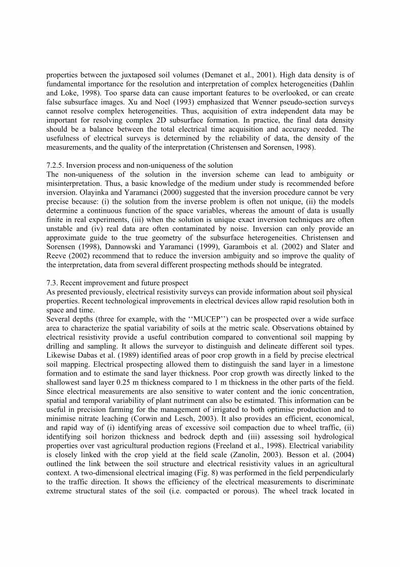
properties between the juxtaposed soil volumes (Demanet et al., 2001). High data density is of fundamental importance for the resolution and interpretation of complex heterogeneities (Dahlin and Loke, 1998). Too sparse data can cause important features to be overlooked, or can create false subsurface images. Xu and Noel (1993) emphasized that Wenner pseudo-section surveys cannot resolve complex heterogeneities. Thus, acquisition of extra independent data may be important for resolving complex 2D subsurface formation. In practice, the final data density should be a balance between the total electrical time acquisition and accuracy needed. The usefulness of electrical surveys is determined by the reliability of data, the density of the measurements, and the quality of the interpretation (Christensen and Sorensen, 1998). 7.2.5. Inversion process and non-uniqueness of the solution The non-uniqueness of the solution in the inversion scheme can lead to ambiguity or misinterpretation. Thus, a basic knowledge of the medium under study is recommended before inversion. Olayinka and Yaramanci (2000) suggested that the inversion procedure cannot be very precise because: (i) the solution from the inverse problem is often not unique, (ii) the models determine a continuous function of the space variables, whereas the amount of data is usually finite in real experiments, (iii) when the solution is unique exact inversion techniques are often unstable and (iv) real data are often contaminated by noise. Inversion can only provide an approximate guide to the true geometry of the subsurface heterogeneities. Christensen and Sorensen (1998), Dannowski and Yaramanci (1999), Garambois et al. (2002) and Slater and Reeve (2002) recommend that to reduce the inversion ambiguity and so improve the quality of the interpretation, data from several different prospecting methods should be integrated. 7.3. Recent improvement and future prospect As presented previously, electrical resistivity surveys can provide information about soil physical properties. Recent technological improvements in electrical devices allow rapid resolution both in space and time. Several depths (three for example, with the ‘‘MUCEP’’) can be prospected over a wide surface area to characterize the spatial variability of soils at the metric scale. Observations obtained by electrical resistivity provide a useful contribution compared to conventional soil mapping by drilling and sampling. It allows the surveyor to distinguish and delineate different soil types. Likewise Dabas et al. (1989) identified areas of poor crop growth in a field by precise electrical soil mapping. Electrical prospecting allowed them to distinguish the sand layer in a limestone formation and to estimate the sand layer thickness. Poor crop growth was directly linked to the shallowest sand layer 0.25 m thickness compared to 1 m thickness in the other parts of the field. Since electrical measurements are also sensitive to water content and the ionic concentration, spatial and temporal variability of plant nutriment can also be estimated. This information can be useful in precision farming for the management of irrigated to both optimise production and to minimise nitrate leaching (Corwin and Lesch, 2003). It also provides an efficient, economical, and rapid way of (i) identifying areas of excessive soil compaction due to wheel traffic, (ii) identifying soil horizon thickness and bedrock depth and (iii) assessing soil hydrological properties over vast agricultural production regions (Freeland et al., 1998). Electrical variability is closely linked with the crop yield at the field scale (Zanolin, 2003). Besson et al. (2004) outlined the link between the soil structure and electrical resistivity values in an agricultural context. A two-dimensional electrical imaging (Fig. 8) was performed in the field perpendicularly to the traffic direction. It shows the efficiency of the electrical measurements to discriminate extreme structural states of the soil (i.e. compacted or porous). The wheel track located in

between the 0.40–0.95 m and 2.3–2.75 m in the first 0.15 m and the plough pan located in the 0.25–0.30 m were distinguished by their low value of resistivity and corresponded to compacted zones (1.53 Mg m-3), as compared to the more porous zones (1.39 Mg m-3). Below 0.30 m, the low resistivity values corresponded of the B horizon.

Fig. 8. Two-dimensional electrical resistivity image perpendicular in the traffic direction (after Besson et al., 2004). Electrical resistivity devices and inversion softwares are currently available on the market. Nevertheless, the primary results obtained after electrical surveys give only indirect information. The method needs primary calibration at the laboratory and interpretations require a minimum knowledge of the medium under study. The use of this method as a routine operation for farmers would appear to be unlikely. The duration of data acquisition is shortened with newly available dataloggers and multiplexers. Such equipment is necessary to perform 3D measurements with a high spatial resolution or to apply electrical resistivity measurements to transfer processes. Landscape solute transport modelling can serve as a crucial component of precision agriculture by providing feedback concerning solute loading to ground-water or to drainage tile systems (Corwin and Lesch, 2003). Christensen and Sorensen (1998) estimated the vulnerability of an aquifer to leakage of a polluting substance from the soil surface, such as infiltration of nitrates from excess fertilisers. These studies constitute a useful step in the hydrological understanding of chemical pollutant transfers such as heavy chemical products released from agricultural and industrial practices. Indeed, salinity limits water uptake by plants by reducing the osmotic potential and thus the available water content for the plant growth. Real-time measurements obtained by electrical resistivity surveys may assist in our understanding of the transport phenomena of water solution and his spatial distribution. Model predictions may help identify management actions that will prevent the occurrence of detrimental conditions. 8. Conclusion Electrical resistivity prospecting is a very attractive method for soil characterisation. Contrary to classical soil science measurements and observations which perturb the soil by random or by regular drilling and sampling, electrical resistivity is non-destructive and can provide continuous measurements over a large range of scales. In this way, temporal variables such as water and plant nutriment, depending on the internal soil structure, are monitored and quantified without altering the soil structure. The applications are numerous: (i) determination of soil horizonation

and specific heterogeneities, (ii) follow-up of the transport phenomena, (iii) monitoring of solute plume contamination in a saline or waste context. It enables the improvement of our understanding of the soil structure and its functioning in varying fields such as agronomy, pedology, geology, archaeology and civil engineering. Concerning agronomy, applications are present in precision farming surveys. Nevertheless, electrical measurements do not give a direct access to soil characteristics that interest the agronomist. Preliminary laboratory calibration and qualitative or quantitative data (i.e. after inversion) interpretations have to be done to link the electrical measurements with the soil characteristics and function. Acknowledgement : The authors gratefully thank Setphen Cattle for improving the English. References Aaltonen, J., 2001. Seasonal resistivity variations in some different swedisch soils. Eur. J. Environ. Eng. Geophys. 6, 33–45. Abdelatif, M.A., Sulaiman, W.N., 2001. Evaluation of groundwater and soil pollution in a landfill area using electrical resistivity imaging survey. Environ. Manag. 28, 655–663. Acworth, R.I., 1999. Investigation of dryland salinity using the electrical image method. Aust. J. Soil Res. 37, 623–636. al Hagrey, S.A., Schubert-Klempnauer, T., Wachsmuth, D., Michaelsen, J., Meissner, R., 1999. Preferential flow: first result of a full-scale flow model. Geophys. J. Int. 138, 643–654. Andrews, R.J., Barker, R., Loke, M.H., 1995. The application of electrical tomography in the study of the unsatured zone in chalk at three sites in Cambridgeshire, United Kingdom. Hydrogeol. J. 3, 17–31. Archie, G.E., 1942. The electrical resistivity log as an aid in determining some reservoir characteristics. Trans. AM. Inst. Min. Metall. Pet. Eng. 146, 54–62. Banton, O., Seguin, M.K., Cimon, M.A., 1997. Mapping field scale physical properties of soil with electrical resistivity. Soil Sci. Soc. Am. J. 61, 1010–1017. Benderitter, Y., Schott, J.J., 1999. Short time variation of the resistivity in an unsaturated soil: the relationship with rainfall. Eur. J. Environ. Eng. Geophys. 4, 37–49. Bernstone, C., Dahlin, T., Ohlsson, T., Hogland, W., 1998. DCresistivity mapping of internal landfill structures: two pre-excavation surveys. Environ. Geol. 39, 360–371. Bertrand, Y., 1967. La prospection électrique appliquée aux problèmes des Ponts et Chaussées. Bulletin Liaison des Laboratoires Routiers Paris – XV. Besson, A., Cousin, I., Samoue¨lian, A., Boizard, H., Richard, G., 2004. Structural heterogeneity of the soil tilled layer as characterized by 2-D electrical resistivity surveying. Soil Till. Res. 79, 239–249. Bevan, B.W., 2000. An early geophysical survey at Williamsburg, USA. Archae. Prospec. 7, 51–58. Binley, A., Cassiani, G., Middelton, R., Winship, P., 2002. Vadose zone flow model parameterisation using cross-borehole radar and resistivity imaging. J. Hydrol. 267, 147–159. Binley, A., Shaw, B., Henry-Poulter, S., 1996. Flow pathways in porous media: electrical resistance tomography and dye staining image verification. Meas. Sci. Technol. 7, 384–390. Bottraud, J.C., Bornand, M., Servat, E., 1984a. Mesures de résistivité appliquées à la cartographie en pédologie. Sci. du Sol 4, 279–294. Bottraud, J.C., Bornand, M., Servat, E., 1984b. Mesures de résistivité et étude du comportement agronomique d’un sol. Sci. Du Sol 4, 295–308.

Bourennane, H., King, D., Le Parco, R., Isambert, M., Tabbagh, A., 1998. Three-dimensional analysis of soils and surface materials by electrical resistivity survey. Eur. J. Environ. Eng. Geophys. 3, 5–23. Brunner, I., Friedel, S., Jacobs, F., Danckwardt, E., 1999. Investigation of a tertiary maar structure using three-dimensional resistivity imaging. Geophys. J. Int. 139, 771–780. Busby, J.P., 2000. The effectiveness of azimuthal apparent-resistivity measurements as a method for determining fracture strike orientations. Geophys. Prospec. 48, 677–695. Butler, J., Roper, T.J., Clark, A.J., 1994. Investigation of badger setts using soil resistivity measurments. Zool. Soc. Lond. 232, 409–418. Campbell, R.B., Bower, C.A., Richards, L.A., 1948. Change of electrical conductivity with temperature and the relation of osmotic pressure to electrical conductivity and ion concentration for soil extracts. Soil Sci. Soc. Proc. 66–69. Chambers, J., Oglivy, R., Meldrum, P., Nissen, J., 1999. 3D resistivity imaging of buried oil- and tar-contaminated waste deposits. Eur. J. Environ. Eng. Geophys. 4, 3–15. Chambers, J.E., Oglivy, R.D., Kuras, O., Cripps, J.C., Meldrum, P.I., 2002. 3D electrical imaging of known targets at a controlled environmental test site. Environ. Geol. 41, 690–704. Choudhury, K., Saha, D.K., Chakraborty, P., 2001. Geophysical study for saline water intrusion in a coastal alluvial terrain. J. Appl. Geophys. 46, 189–200. Christensen, B.N., Sorensen, K., 1998. Surface and borehole electric and electomagnetic methods for hydrological investigation. Eur. J. Environ. Eng. Geophys. 3, 75–90. Colman, E.A., Hendrix, T.M., 1949. The fiberglas electrical soil moisture instrument. Soil Sci. 67, 425–438. Corwin, D.L., Lesch, S.M., 2003. Application of soil electrical conductivity to precision agriculture: theory, principles, and guidelines. Agron. J. 95, 455–471. Dabas, M., Hesse, A., Jolivet, A., Tabbagh, A., 1989. Intérêt de la cartographie de la résistivité électrique pour la connaissance du sol à grande échelle. Sci. du Sol 27, 65–68. Dabas, M., Tabbagh, A., Tabbagh, J., 1994. 3D inversion in subsurface electrical surveying-I. Theory Geophys. J. Int. 119, 975–990. Dahlin, T., 2000. Short note on electrode charge-up effects in DC resistivity data acquisition using multi-electrode arrays. Geophys. Prospec. 48, 181–187. Dahlin, T., Loke, M.H., 1998. Resolution of 2D Wenner resistivity imaging as assessed by numerical modelling. J. Appl. Geophys. 38, 237–249. Dannowski, G., Yaramanci, U., 1999. Estimation of water content and porosity using radar and geoelectrical measurements. Eur. J. Environ. Eng. Geophys. 4, 71–85. Demanet, D., Renardy, F., Vanneste, K., Jongmans, D., Camelbeeck, T., Meghraoui, M., 2001. Case History The use of geophysical prospecting for imaging active faults in the Roer Graben, Belgium. Geophysics 66, 78–89. Depountis, N., Harris, C., Davies, M.C.R., 2001. An assessment of miniaturised electrical imaging equipment to monitor pollution plume evolution in scaled centrifuge modelling. Eng. Geol. 60, 83–94. Dey, A., Morrison, H.F., 1979. Resistivity modelling for arbitrarily shaped three-dimensional structures. Geophysics 44, 753–780. Edwards, L.S., 1977. A modified pseudosection for resistivity and IP. Geophysics 42, 1020–1036. Freeland, R.S., Yoder, R.E., Ammons, J.T., 1998. Mapping shallow underground features that influence site-specific agricultural production. J. Appl. Geophys. 40, 19–27.

Frohlich, R.K., Parke, C.D., 1989. The electrical resistivity of the Vadose Zone – Field Survey. Ground Water 27, 524–530. Frohlich, R.K., Urish, D.W., Fuller, J., O’Reilly, M., 1994. Use of geoelectrical methods in groundwater pollution surveys in a coastal environment. J. Appl. Geophys. 32, 139–154. Fukue, M., Minatoa, T., Horibe, H., Taya, N., 1999. The microstructure of clay given by resistivity measurements. Eng. Geol. 54, 43–53. Garambois, S., Senechal, P., Perroud, H., 2002. On the use of combined geophysical methods to assess water content and water conductivity of near-surface formations. J. Hydrol. 259, 32–48. Giao, P.H., Chung, S.G., Kim, D.Y., Tanaka, H., 2003. Electric imaging and laboratory resistivity testing for geotechnical investigation of Pusan clay deposits. J. Appl. Geophys. 52, 157–175. Goyal, V.C., Gupta, P.K., Seth, P.K., Singh, V.N., 1996. Estimation of temporal changes in soil moisture using resistivity method. Hydrol. Process. 10, 1147–1154. Griffiths, D.H., Barker, R.D., 1993. Two-dimensional resistivity imaging and modelling in areas of complex geology. J. Appl. Geophys. 29, 211–226. Guérin, R., Pannissod, C., Thiry, M., Benderitter, Y., Tabbagh, A., Huet-Tailanter, S., 2002. La friche industrielle de Mortagne-du-Nord (59) – III – Approche me´thodologique d’étude géophysique non-destructive des sites pollués par des eaux fortement minéralisées. Bull. Soc. Geol. Fr. 173, 471–477. Gupta, S.C., Hanks, R.J., 1972. Influence of water content on electrical conductivity of the soil. Soil Sci. Soc. Am. Proc. 36, 855–857. Habberjam, G.M., Watkins, G.E., 1967. The use of a square configuration in resistivity prospecting. Geophys. Prospec. 15, 445–467. Hallof, P.G., 1957. On the interpretation of resistivity and induced polarization measurements. Ph.D Thesis, Massachusetts, 256 pp. Hesse, A., Jolivet, A., Tabbagh, A., 1986. New prospects in shallow depth electrical surveying for archeological and pedological applications. Geophysics 51, 585–594. Jackson, P.D., Northmore, K.J., Meldrum, P.I., Gunn, D.A., Hallam, J.R., Wambura, J., Wangusi, B., Ogutu, G., 2002. Non-invasive moisture monitoring within an earth embankment – a precursor to failure. NDT&E Int. 35, 107–115. Jones, J.W., 1995. Scale-dependent resistivity measurements of oracle granite. Geophys. Res. Lett. 22, 1453–1456. Kalinski, R.J., Kelly, W.E., 1993. Estimating Water Content of soils from electrical resistivity. Geotech. Test. J. 16, 323–329. Kampke, A., 1999. Focused imaging of electrical resistivity data in archaeological prospecting. J. Appl. Geophys. 41, 117–215. Karlik, G., Kaya, M.A., 2001. Investigation of groundwater contamination using electric and electromagnetic methods at an open waste-disposal site: a case study from Isparta. Turkey Environ. Geol. 40, 725–731. Kearey, P., Brooks, M., Hill, I., 2002. An introduction to geophysical exploration. Blackwell Science. Kemna, A., Vanderborght, J., Kulessa, B., Vereecken, H., 2002. Imaging and characterisation of subsurface solute transport using electrical resistivity tomography (ERT) and equivalent transport models. J. Hydrol. 167, 125–146. Lamotte, M., Bruand, A., Dabas, M., Donfack, P., Gabalda, G., Hesse, A., Humbel, F.-X., Robain, H., 1994. Distribution d’un horizon à forte cohésion au sein d’une couverture de sol aride du Nord-Cameroun : apport d’une prospection électrique. Comptes Rendus à l’Académie des Sciences. Earth Planet. Sci. 318, 961–968.

Lane, J.W., Haeni, F.P., Watson, W.M., 1995. Use of a square-array direct-current resistivity, method to detec fractures in crystalline Bedrock in New Hampshire. Ground Water 33, 476–485. Lataste, J.F., Breysse, D., Sirieix, C., Frappa, M., Bournazel, J.P., 2002. Fissuration des ouvrages en béton armé Auscultation par mesure de résistivité électrique. Bull. Lab. Ponts et Chaussées 239, 79–91. Lile, O.B., Backe, H.R., Elvebakk, H., Buan, J.E., 1994. Resistivity measurements on the sea bottom to map fractures zones in the bedrock underneath sediments. Geophys. Prospec. 42, 813–824. Loke, M.H., 2001. Tutorial: 2-D and 3-D electrical imaging surveys.Course Notes for USGS Workshop 2-D and 3-D Inversion and Modeling of Surface and Borehole Resistivity Data, Torrs, CT. Loke, M.H., Barker, R.D., 1996. Rapid least-squares inversion of apparent resistivity pseudosections using a quasi-Newton method. Geophys. Prospec. 44, 131–152. Mauriello, P., Monna, D., Patella, D., 1998. 3D geoelectric tomography and archaeological applications. Geophys. Prospec. 46, 543–570. McCarter, W.J., 1984. The electrical resistivity characteristics of compacted clays. Ge´otechnique 34, 263–267. Meheni, Y., Gue´rin, R., Benderitter, Y., Tabbagh, A., 1996. Subsurface DC resistivity mapping: approximate 1-D interpretation. J. Appl. Geophys. 34, 255–270. Meyer de Stadelhofen, C., 1991. Application de la géophysique aux recherches d’eau. Ed. Lavoisier, Paris. Michot, D., Benderitter, Y., Dorigny, A., Nicoullaud, B., King, D., Tabbagh, A., 2003. Spatial and temporal monitoring of soil water content with an irrigated corn crop cover using electrical resistivity tomography. Water Resour. Res. 39, 1138. Michot, D., Dorigny, A., Benderitter, Y., 2000. Mise en évidence par résistivité électrique des écoulements préférentiels et de l’assèchement par le maıs d’un calcisol de Beauce irrigué. C.R. Acad. Sci. 332, 29–36. Nowroozi, A.A., Horrocks, S.B., Henderson, P., 1999. Saltwater intrusion into the freshwater aquifer in the eastern shore of Virginia: a reconnaissance electrical resistivity survey. J. Appl. Geophys. 42, 1–22. Oglivy, R., Meldrum, P., Chambers, J., 1999. Imaging of industrial waste deposits and buried quarry geometry by 3-D resistivity tomography. Eur. J. Environ. Eng. Geophys. 3, 103–113. Olayinka, A.I., Yaramanci, U., 2000. Assessment of the reliability of 2D inversion of apparent resistivity data. Geophys. Prospec. 48, 293–316. Oldenburg, D.W., Li, Y., 1994. Inversion of induced polarization data. Geophysics 59, 1327–1341. Olsen, P.A., Binley, A., Henry-Poulter, S., Tych, W., 1999. Characterizing solute transport in undisturbed soil cores using electrical and X-ray tomographic methods. Hydrol. Process. 13, 211–221. Palacky, G.J., 1987. Clay mapping using electromagnetic methods. First Break 5, 295–306. Panissod, C., Dabas, M., Jolivet, A., Tabbagh, A., 1997a. A novel mobile multipole system (MUCEP) for shallow (0–3 m) geoelectrical investigation: the ’Vol-de-Canards’ array. Geophys. Prospec. 45, 983–1002. Panissod, C., Lajarthe, M., Tabbagh, A., 1997b. Potential focusing : a new multielectrode array concept, simulation study and field tests in archaeological prospecting. J. Appl. Geophys. 38, 1–23.

Park, S., 1998. Fluid migration in the vadose zone from 3-D inversion of resistivity monitoring data. Geophysics 63, 41–51. Pettinen, S., Sutinen, R., Ha¨nninen, P., 1999. Determination of anisotropy of tills by means of azimuthal resistivity and conductivity measurements. Nord. Hydrol 30, 317–332. Pozdnyakova, L., Pozdnyakov, A., Zhang, R., 2001. Application of geophysical methods to evaluate hydrology and soil properties in urban areas. Urban Water 3, 205–216. Reynolds, J.M., 1997. An Introduction to Applied and Environmental Geophysics. Wiley. Rhoades, J.D., van Schilfgaarde, J., 1976a. An electrical conductivity probe for determining soil salinity. Soil Sci. Soci. Am. J. 40, 647–651. Rhoades, J.D., Kaddah, M.T., Halvorson, A.D., Prather, R.J., 1977. Establishing soil electrical conductivity salinity calibration using four electrodes cells containing undisturbed soil cores. Soil Sci. 123, 137–141. Rhoades, J.D., Raats, P.A.C., Prather, R.J., 1976b. Effect of liquid phase electrical conductivity, water content, and surface conductivity on bulk soil electrical conductivity. Soil Sci. Soci. Am. J. 40, 651–655. Ritz, M., Robain, H., Pervago, E., Albouy, Y., Camerlynck, C., Descloitres, M., Mariko, A., 1999. Improvement to resistivity pseudosection modelling by removal of near-surface inhomogeneity effects: application to a soil system in south Cameroon. Geophys. Prospec. 47, 85–101. Robain, H., Descloitres, M., Ritz, M., Atangana, Q.Y., 1996. A multiscale electrical survey of a lateritic soil system in the rain forest of Cameroon. J. Appl. Geophys. 34, 237–253. Robain, H., Lajarthe, M., Florsch, N., 2001. A rapid electrical sounding method The ‘‘three-point’’ method: a Bayesian approach. J. Appl. Geophys. 47, 83–96. Samouelian, A., Cousin, I., Richard, G., Tabbagh, A., Bruand, A., 2003. Electrical resistivity imaging for detecting soil cracking at the centimetric scale. Soil Sci. Soc. J. Am. 67, 1319–1326. Sandberg, S.K., Slater, L.D., Versteeg, R., 2002. An intergrated geophysical investigation of the hydrogeology of an anisotropic unconfined aquifer. J. Hydrol. 267, 227–243. Schlumberg, 1989. Log Interpretation Charts. Well Science, Houston. Scollar, I., Tabbagh, A., Hesse, A., Herzog, I., 1990. Archaeological Prospecting and Remote Sensing. , 674 pp. Seaton, W.J., Burbey, T.J., 2002. Evaluation of two-dimensional resistivity methods in a fractured crystalline-rock terrane. J. Appl. Geophys. 51, 21–41. Senos Matias, M.J., 2002. Square array anisotropy measurments and resistivity souding interpretation. J. Appl. Geophys. 49, 185–194. Shaaban, F.F., Shaaban, F.A., 2001. Use of two-dimensional electric resistivity and ground penetrating radar for archaeological prospecting at the ancient capital of Egypt. J. Afr. Earth Sci. 33, 661–671. Sharma, P.V., 1997. Environmental and Engineering Geophysics. Cambridge University Press. Shea, P.F., Luthin, J.N., 1961. An investigation of the use of the fourelectrode probe for measuring soil salinity in situ. Soil Sci. 92, 331–339. Slater, L., Binley, A., Versteeg, R., Cassiani, G., Birken, R., Sandberg, S., 2002. A 3D ERT study of solute transport in a large experimental tank. J. Appl. Geophys. 49, 211–229. Slater, L., Binley, A.M., Daily, W., Johnson, R., 2000. Cross-hole electrical imaging of a controlled saline tracer injection. J. Appl. Geophys. 44, 85–102. Slater, L., Reeve, A., 2002. Investigation peatland stratigraphy and hydrogeology using integrated electrical geophysics. Geophysics 67, 365–378.

Slater, L.D., Binley, A., Brown, D., 1997. Electrical imaging of fractures using ground-water salinity change. Ground Water 35, 436–442. Tabbagh, A., 1985. The response of a three-dimensional magnetic and conductive body in shallow depth electromagnetic prospecting. Geophys. J.R. Astr. Soc. 81, 215–230. Tabbagh, A., Dabas, M., Hesse, A., Panissod, C., 2000. Soil resistivity: a non-invasive tool to map soil structure horizonation. Geoderma 97, 393–404. Van Dam, J.C., Meulenkamp, J.J., 1967. Some results of the geoelectrical resistivity method in groundwater investigations in the Netherlands. Geophys. Prospec. 15, 92–115. White, P.A., 1988. Measurement of ground-water parameters using salt-water injection and surface resistivity. Ground Water 26, 179–186. White, P.A., 1994. Electrode arrays for measuring groundwater flow direction and velocity. Geophysics 59, 192–201. Xu, B., Noel, M., 1993. On the completeness of data sets with multielectrode systems for electrical resistivity survey. Geophys. Prospec. 41, 791–801. Yaramanci, U., 2000. Geoelectric exploration and monitoring in rock salt for the safety assessment of underground waste disposal sites. J. Appl. Geophys. 44, 181–196. Yoon, G.L., Park, J.B., 2001. Sensitivity of leachate and fine contents on electrical resistivity variations of sandy soils. J. Hazard. Mater. 84, 147–161. Zanolin, A., 2003. Irrigation de precision en Petite-Beauce: mesures au champ et modélisation stochastique spatialisée du fonctionnement hydrique et agronomique d’une parcelle de maıs, Paris VI. Paris, 187 pp. Zhou, Q.Y., Shimada, J., Sato, A., 2001. Three-dimensional spatial and temporal monitoring of soil water content using electrical resistivity tomography. Water Resour. Res. 37, 273–285.