electrical resistivity as a tool for analyzing soil gas...

1

Sara Johansson

2009

Master of Science project

Department of Physics

Lund University

Sölvegatan 14C

S-223 62 Lund

Sweden

Electrical resistivity as a tool for

analyzing soil gas movements & gas emissions from landfill soils

2

ELECTRICAL RESISTIVITY AS A TOOL FOR ANALYSING SOIL GAS MOVEMENTS & GAS EMISSIONS FROM LANDFILL

SOILS

Master of Science Project in collaboration with Tyréns AB

_____________________________________________________________________

Sara Johansson 2009

Master of Science Project in Physics and Physical Geography

Supervisors

Anna Ekberg

Department of Physical Geography & Ecosystem Analysis

Harry Lankreijer

Department of Physical Geography & Ecosystem Analysis

Mats Svensson

Tyréns AB

3

ABSTRACT

The aim of this thesis is to evaluate if the geophysical method electrical resistivity can be used as a tool to analyse gas movements in and gas emissions from heterogeneous soils such as landfills. Electrical resistivity is a material parameter that describes the isolative capacity of the ground; consequently a large amount of water in the soil pores conveys low resistivity values in the soil model. Analogously, a large amount of gas present in the soil pores is assumed to bring high resistivity values. Increasing soil moisture during the investigation period of 5 days could be indicated at some of the measurement plots as a decreace in the residual variation in resistivity, as well as decreasing CH4 flux in accordance with litterature. Larger rain events was detected in five of six measurement plots as negative peeks in resistivity in the surface soil layers, where after an immediate pronounced peak in occured. This was interpreted as gas advection; initially gas is forced downwards into deeper soil layers during the rain event, where after the gas is forced upwatds when the water is infiltrated into deeper soil layers. Simoultaneously with these resistivity peaks, maximum CH4 fluxes were measured at three of six measurement plots, suggesting a release of CH4 from the landfill soil through gas advection after rain events. The overall picture of the gas movements at the landfill was that the extention of gas assimilations increased and decreased following the diurnal variation in soil temperature; simoultaneously with soil temperature, maximum peaks in resistivity could be seen, perhaps linked to high gas pressure according to the ideal gas law. Electrical resistivity seems to be helpful in analysing the spatially and temporally varying CH4 fluxes from landfills, but more research and an adjustment of the methodology is needed to stress the results.

SUMMARY

The anaerobic production and emissions of CH4 from landfills is an environmental problem that is hard to predict and mitigate, since the soil structure and waste composition of landfills are highly heterogeneous. Soil gas moves through molecular diffusion driven by concentration gradients, or through advection determined by pressure gradients. According to literature, the gas generally moves in horizontal directions in landfills, since the soil consist of packed layers with a higher horizontal than vertical permeability.

The aim of this study is to evaluate if the geophysical method electrical resistivity can be used in combination with measurements of surface gas emissions, in order to obtain better knowledge of gas behaviour in landfill soils as well as their relation to the highly spatial and temporal variability of gas emissions from landfills.

The principle of electrical resistivity measurements is to let an electric current pass through the soil between two electrodes. In two additional electrodes, the potential of the ground is measured. From the measured potential, the strength of the current and the spacing between the electrodes, the apparent resistivity can be calculated, assuming that the soil is homogeneous (which is seldom the case in reality). Through data inversion, models of the soil are created, with distribution of true resistivity values in different layers and areas of the ground.

The material property resistivity is, unlike resistance, independent on dimensions of the soil volume that the current flows through. The resistivity values of the ground are related to material, but also to the amount of water or air in the soil pores. With a lot of water present in the soil, the resistivity becomes low and in analogy with this, the resistivity is expected to rise when the soil pores consist of a lot of gas. The

4

central assumption used here is that when looking at changes in resistivity over time, the main changes depends on the relative amount of gas or water in the soil pores.

The current study was made in the frames of a research project lead by Tyréns AB, NSR Återvinning and Lund University. The study location was a 20x18m area upon the landfill Filborna in Helsingborg. Electrical resistivity was systematically measured with the ABEM Lund Imaging System, an automatic system that provided resistivity models every second hour during June-September 2008. Climatic variables were logged every minute with a Campbell C1000 data logger, and soil moisture was measured occasionally in twelve TDR-probes with a TDR100-instrument. Static chamber measurements of CH4 fluxes from the surface were measured at six fixed measurement plots during two of the field weeks (4th-11th of July and 18th-22nd of August) and analysed in a gas chromatograph with a FID-detector.

The resistivity data was imported in Matlab, and the resistivity in three different soil layers below each static chamber measurement plot was interpolated and plotted on a time-axis. Soil temperature had an effect on resistivity through affecting the conductivity of the soil, which is described with an empirical relationship found in the literature. This temperature effect was modelled by using the soil temperature from the weather station, and withdrawn from the measured resistivity variations.

The resulting graphs showed that the changes in resistivity at all measurement plots more or less followed the diurnal variations in soil temperature. This was proposed as an effect of gas pressure following soil temperature according to the ideal gas law. Another observation was that the resistivity decreased during three larger rain events, where after the resistivity often rose to considerable peaks in resistivity. At some of the plots, maximum CH4 fluxes occurred simultaneously with the resistivity peaks, while the flux data at other plots were insufficient to stress this relationship. However, from what could be seen, this behaviour was consistent at all plots except one, and it was interpreted as a result of gas advection from the soil; when the water infiltrated to deeper soil layers after the rain event, it is possible that the gas present in the soil pores was forced upwards and resulted in larger fluxes.

The effect of continuously increasing soil moisture during the week was also indicated in some of the graphs, since the resistivity steadily decreased during the week at this plots. Also the CH4 flux tended to decrease during the week at two of the plots (with the advection fluxes excluded), an expected result since water in the upper soil layers blocks the gas from being diffusing to the atmosphere.

At some of the measurement plots, several of the CH4 fluxes were negative. This probably means that CH4 oxidation in the upper soil layers occured here, as a result of oxygen present in the soil pores. Landfill gas consists in addition to CH4 of approximately 50% CO2, but this constituent was not analysed. To improve this method, it would be preferable to analyse not only the CH4 but also the CO2 flux, among other reasons to obtain a more accurate analysis of the CH4 oxidation. More replicates of gas flux measurements are necessary to stress the results and conclusions from this study.

Although the field method could be improved, the conclusion of this study is that it can be valuable to use electrical resistivity for analysing gas behaviour and their relation to surface emissions at landfills. The resistivity data must be interpreted with care, since technical effects and uncertainty can cause problems when looking at the data on a small scale. The resistivity measurement can visualize gas presence and movements in the soil. In combination with flux measurements, it has lead to the suggestion that relatively large gas emissions are likely to occur at different locations around the landfill as a consequence of advection flow after larger rain events. In

5

addition, diffusion flux occurs and is coupled to soil moisture and soil temperature. The average fluxes are higher in the vincinity of gas assimilations in the soil. Hopefully, studies of this kind can improve the knowledge of the reason for the spatially and temporally varying fluxes from landfills.

PREFACE

This master degree project was performed as a part of a research project lead by

Tyréns AB, NSR Återvinning and Lund University. The main objective of the research project was to investigate if it is possible to detect gas assimilations in landfills with electrical resistivity.

ACKNOWLEDGEMENTS

I would like to thank my supervisors Mats Svensson at Tyréns AB and Harry

Lankreijer and Anna Ekberg at the Department of Physical Geography & Ecosystem Analysis at Lund University. I would also like to thank Håkan Rosqvist for reading and commenting on my report, as well as Torleif Dahlin, Virginie Leroux, Magnus Lindsjö and Carl-Henrik Månsson for discussions and coorperation in the project and their guidance regarding their special knowledge. Finally, I would like to thank everyone else who have helped me in any way with this project.

6

CONTENTS Abstract……………………………………………………………………………....3 Summary……………………………………………………………………………..3 Preface………………………………………………………………………………..5 Acknowledgements…………………………………………………………………..5 Contents……………………………………………………………………….……...6

1. INTRODUCTION……………………………………………….9 1.1 BACKGROUND…………………………………………………………...…9 1.2 AIM & OBJECTIVES……………………………………………………… 11

2. THEORY………………………………………………………..12 2.1 ELECTRICAL RESISTIVITY………………………………………………12 2.1.1 General principle of electrical resistivity measurements……………...…12 2.1.2 The resistivity model…………………………………………………….14 2.1.3 Resistivity data interpretation…………………………………………....15 2.1.4 Landfill research with electrical resistivity………………………………16 2.2 LANDFILL GAS TRANSPORT……………………………………………17 2.2.1 Landfill gas………………………………………………………………17 2.2.2 General about gas transport in landfills………………………………….18 2.2.3 Soil conditions…………………………………………………………...19 2.2.4 Soil gas diffusion………………………………………………………...19 2.2.5 Soil gas advection………………………………………………………..20

3. EXPERIMENTAL METHODS & MATERIALS……………21

3.1 SITE DESCRIPTION & MEASUREMENT PERIOD……………………...21 3.2 ELECTRICAL RESISTIVITY SETUP……………………………………..22 3.3 SURFACE CH4 FLUX………………………………………………………23

3.3.1 Static gas chamber measurements……………………………………….23 3.3.2 Lab analysis and flux calculations……………………………………….25 3.3.3 Uncertainty in the flux data………………………………………………26 3.4 ENVIRONMENTAL VARIABLES………………………………………...26 3.4.1 Soil temperature………………………………………………………….26 3.4.2 Soil moisture……………………………………………………………..26 3.4.3 Weather station…………………………………………………………..27

7

4. DATA ANALYSIS METHODS……………………………….28 4.1 TIME-LAPS ANALYSIS OF RESISTIVITY DATA…………………….28

4.2 VARIATIONS IN CH4 FLUX DATA…………………………………….33

4.3 SOIL GAS DIFFUSION AND ADVECTION……………………………33

5. RESULTS……………………………………………………….34 5.1 VARIATION IN CH4 FLUXES…………………………………………….34 5.2 CH4 FLUXES AND VARIATION IN RESISTIVITY……………………...35

5.2.1 Plot K1…………………………………………………………………...35 5.2.2 Plot K2…………………………………………………………………...38 5.2.3 Plot K3…………………………………………………………………...41 5.2.4 Plot K4………………………………………………………………..….43 5.2.5 Plot K5…………………………………………………………………...45 5.2.6 Plot K6…………………………………………………………………...47

5.3 SOIL DIFFUSION COEFFICIENT………………………………………....49 5.4 INFILTRATING WATER, SOIL GAS AND FLUXES……………….…....50

6. DISCUSSION…………………………………………………...53 6.1 THE TEMPERATURE INFLUENCE ON SOIL GAS AND FLUXES…….53

6.2 NEGATIVE CH4 FLUXES…………………………………………………..53

6.3 BEHAVIOR OF GAS FLUXES AT LANDFILLS…………………………54

6.4 UNCERTAINTIES IN THE ANALYSIS OF THE RESISTIVITY DATA...55

6.5 UNCERTAINTY OF THE RESULTS………………………………………57

6.6 FUTURE IMPROVEMENTS OF THE METHODOLOGY………………..58

7. CONCLUSIONS………………………………………………..59

8. REFERENCES……………………………………………….…60

9

1. INTRODUCTION 1.1 BACKGROUND

Landfills fulfil the function of being the final deposit of wastes that cannot be used

for any beneficial purpose. Many landfills in Sweden have been used for decades, and have continuously been increased with new deposits. When they have earned out their purpose, landfills pass to a phase during which active preservations of environment are still necessary. Such preservations could for example be to cover them with clay or plastics to reduce gas emissions. When the emissions from landfills become small enough not to significantly impact the environment, the active custody of them can be terminated. Some of these landfills have been covered and are now overlain by forests, settlements etc. (Christensen 1998).

Waste hierarchy is a basic concept used in waste technology, referring to the ideal values of and management of refuse. Directions from the European Union from 1999 suggest a waste hierarchy that is also recommended by SEPA; the Swedish environmental protection agency (Naturvårdsverket 1). The significance of the EU waste hierarchy is to prioritize waste management methods according to:

I. Prevention or minimization of waste II. Re-utilization

III. Recycling IV. Safe custody of waste

The deposit of waste into landfills ends up under number IV on the hierarchy

above, and is conceivable only when there can be no further use of the refuse (Naturvårdsverket 1). The fourth prioritized alternative, Safe custody of waste, is in other versions of the waste hierarchy (and in practice) divided into the higher prioritized Combustion and energy usage, and the least conceivable alternative of Deposition (Christensen 1998).

The overall goal for deposition as a waste management method is to reduce the amounts of waste deposited in landfills as much as possible. Waste that still has to be deposited will in the future probably be concentrated to fewer landfills with higher standard. The EU directives from 1999 have already led to an improved standard of many European landfills, including Swedish, during recent years. Predictions say that 50% of the 500 active landfills in Sweden today will be shut down in the near future. (Naturvårdsverket 2).

The waste that ends up in landfills can have both industrial- and municipal origin. The meaning of the term municipal waste is that it consists of, or is similar in its composition to, household waste (Europeiska Unionens råd 2001). Today, organic material is prohibited in landfills, but SEPA, and the county administration in individual cases, are allowed to make directions about exceptions from this paragraph (Miljödepartementet 2001). It should also be kept in mind that some landfills could contain organic materials from earlier periods, during which the regulations were not as hard as today. Grocery remainders may also not be completely absent in municipal waste.

One of several environmental problems with landfills is concerning the gas emissions to the atmosphere. Landfill gas is produced from the biodegradation of organic material in the waste. When oxygen is available, the main component of the gas produced is CO2 (CO2), while CH4 (methane) is produced under anaerobic

10

conditions. CH4 can also be oxidised to CO2 before it escapes the landfill. The percentage share between CO2 and CH4 in landfill gas at equilibrium is usually around 55% CH4 and 45% CO2, although these figures can vary between sites. In addition, also trace quantities of N2, H2S, gaseous hydrocarbons and other compounds are present in landfill gas (Crawford & Smith 1985). At present day, it is hard to estimate how large the proportion of released CH4 to the atmosphere is compared to the total amount produced in landfills, but figures from Swedish government’s energy authority STEM 2005 suggests that 21-63% of the CH4 produced in Swedish landfills (with a large variation between sites) reaches the atmosphere. Studies from USA have resulted in a corresponding value of 20-50% (Samuelsson et al. 2005).

Both CO2 and CH4 are strong greenhouse gases, but it is the CH4 emissions that are worrying; CH4 has a global warming potential of 25 CO2 equivalents over a time period of 100 years (IPCC, Foster et al. 2007). On a global scale it is a well known fact that emissions of anthropogenic CH4 is about twice as large as natural CH4 emissions, and that landfills is an important anthropogenic CH4 source among for example rice paddies, biomass burning and fermentation in guts of domestic animals (Chapin et al. 2002).

IPCC (UN:s Intergovernmental panel on climate change) conclude in their Fourth Assessment Report from 2007 that the anthropogenic emissions of greenhouse gases (CO2, CH4, N2O and halocarbons) cause the global warming. The atmospheric concentration of CH4 has increased with 30% during the last 25 years. The current atmospheric concentration of CH4 is approximately 1.8ppb, compared to the pre-industrial values of around 0.7ppb in between AD 1700-1800. This corresponds to a radiative forcing (RF) of +0.48Wm-2, which is the second largest RF of all greenhouse gases (CO2 have a RF of +1.66Wm-2). Radiative forcing is a parameter that describes how the energy balance of the earth-atmosphere system is affected by changes in atmospheric concentrations of gases (or by other factors that affects the climate; albedo etc.). A positive RF implies that the energy of the earth-atmosphere system will increase and cause a warming (IPCC Foster et al. 2007).

Consequently, there are two major advantages in trapping and collecting landfill gas; the environmental benefit of reducing the amounts of CH4 emissions to the atmosphere is one of them. Another interest of these activities is economical and social; landfill gas can be refined into biogas, which is used as fuel in vehicles and energy to heat up buildings. Combustion of biogas from landfills has the advantages of being a renewable energy source, unlike for example combustion of fossil fuels, at the same time as it prevents CH4 emissions from landfills (Harbison 2008).

When gas production and gas emissions through soils are modelled in order to estimate greenhouse gas emissions from a natural ecosystem, the soil is often considered as a homogeneous medium, through which the gas migrates upwards through the soil (Fang et al.1999). Several studies have shown that the major controls of the magnitude of the gas emissions are temperature, soil moisture, soil porosity and organic matter content (Fang et al. 1999).

The emissions of landfill gas on the other hand show highly variable spatial and temporal patterns. Even though the processes involved in gas transport inside landfills are known, large uncertainties regarding the actual pattern of gas movements still remains, which is especially convenient in landfill gas models. The uncertainties originate in the structural heterogeneity of landfills; differences in waste composition and compaction bring a large variety in porosity, moisture and hydraulic conductivity across a landfill that is difficult to model without exhaustive excavations (Lamborn 2007).

11

Geophysics is a valuable technique for visualising structures below the earth

surface, and the electrical resistivity method has been used frequently for detecting water migration in landfills. Indications of a possibility also to detect gas inside landfills were recently presented, and during 2008 an investigation project took place at a landfill to inquire into this matter. It is within this project, lead by Tyréns AB and NSR Återvinning among other participators, that the current degree project was performed.

With the indications of a possibility to detect landfill gas with electrical resistivity, the idea of using geophysics as a visual tool for understanding gas behaviour in landfill soils and it’s relation to the varying surface emissions was developed.

A lot of important research is ongoing to understand the reaction of natural and anthropogenic environments to present conditions, as well as a changing climate. Process-based knowledge improves climate modelling of the future and makes preventative measures more efficient. In this perspective, it makes sense to try new methods for understanding gas behaviour in landfills, e.g. with the electrical resistivity method used here. Hopefully the results can provide some clues or inspiration to a better understanding of the highly variable spatial and temporal variations in gas emissions from landfills, which in the future can lead to a reduced amount of greenhouse gases to the atmosphere. 1.2 AIM & OBJECTIVES

The aim of this project is to evaluate if the electrical resistivity method can be used to obtain better knowledge of subsurface gas behaviour and CH4 emissions from landfills.

• Can the gas transport inside the landfill be visualized by resistivity measurements and described theoretically?

• Is there a relationship between weather data, gas behaviour in the soil and CH4 emissions from the surface?

12

2 THEORY

2.1 ELECTRICAL RESISTIVITY

2.1.1 General principle of electrical resistivity measurements

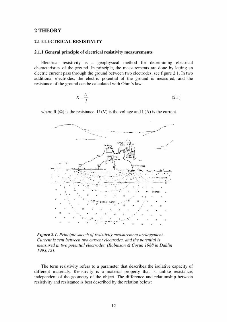
Electrical resistivity is a geophysical method for determining electrical

characteristics of the ground. In principle, the measurements are done by letting an electric current pass through the ground between two electrodes, see figure 2.1. In two additional electrodes, the electric potential of the ground is measured, and the resistance of the ground can be calculated with Ohm’s law:

I

UR = (2.1)

where R (Ω) is the resistance, U (V) is the voltage and I (A) is the current.

The term resistivity refers to a parameter that describes the isolative capacity of

different materials. Resistivity is a material property that is, unlike resistance, independent of the geometry of the object. The difference and relationship between resistivity and resistance is best described by the relation below:

Figure 2.1. Principle sketch of resistivity measurement arrangement.

Current is sent between two current electrodes, and the potential is

measured in two potential electrodes. (Robinson & Coruh 1988 in Dahlin

1993:12).

13

A

dlR ⋅= ρ (2.2)

which defines the resistivity ρ(Ωm) of the material, where R(Ω) is the resistance

for the current through a path of length dl(m) and cross sectional area A(m2) (Parasnis 1986).

If the earth is assumed to be homogeneous, and an electrical current is sent into the ground from a single current electrode, the current will flow radially from the source electrode into the ground. This is true under the conditions that a possible sink electrode for the electrical current is at a large distance from the current source electrode. If the current flows radially into the ground, the cross sectional area of the current path is spherical; A = 2 ⋅ π ⋅ r2 . If expression (2.2) is combined with Ohm’s law, the potentials U at distances r from the current electrode becomes:

22 r

I

r

U

⋅⋅

⋅=

∂

∂

π

ρ (2.3)

That means, that if the current I is known, the resistivity ρ can be calculated in all

points of the ground where the potential U can be measured. In real electrical resistivity measurements, the potential difference ∆U between two potential electrodes is measured instead of the potential U at one single electrode. The reason for this is practical and has to do with measurement techniques. The potential electrodes are placed in the electric field in between the source and sink electrodes (see figure 2.1). The potential measured at each of the potential electrodes C and D is the sum of the contributing potential influence of both current electrodes A and B:

)()( DBDACBCADC UUUUUUU +−+=−=∆ (2.4)

Integration of equation (2.3), and substituting this into equation (2.4) leads to the

following relationship:

−−

−⋅

∆⋅⋅=

DBDACBCA

a

rrrrI

U

1111

2 πρ (2.5)

This is the basic expression for computing the so-called apparent resistivity values

ρa. This equation is clearly dependent on the spacing between the electrodes (Kearey & Brooks 1991).

There are a number of methods with different advantages to choose between when selecting the electrode arrangement and configuration for electrical resistivity measurements. Larger electrode spacing results in a deeper ground penetration of the electric current, but it also means that the resolution of the data decreases with depth (Dahlin 1993).

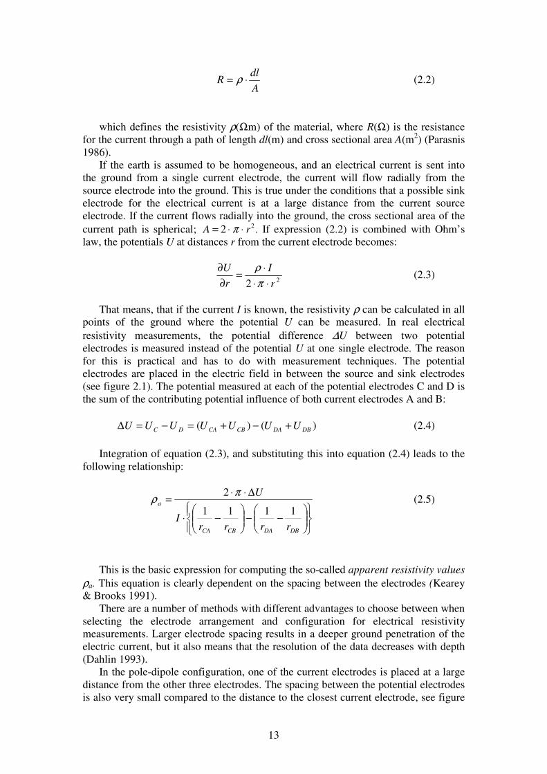
In the pole-dipole configuration, one of the current electrodes is placed at a large distance from the other three electrodes. The spacing between the potential electrodes is also very small compared to the distance to the closest current electrode, see figure

14

2.2. The advantages of this configuration is according to literature that it reduces noise, provides good resolution of horizontal structures and is sensitive to surface inhomogenities (Sharma 1997).

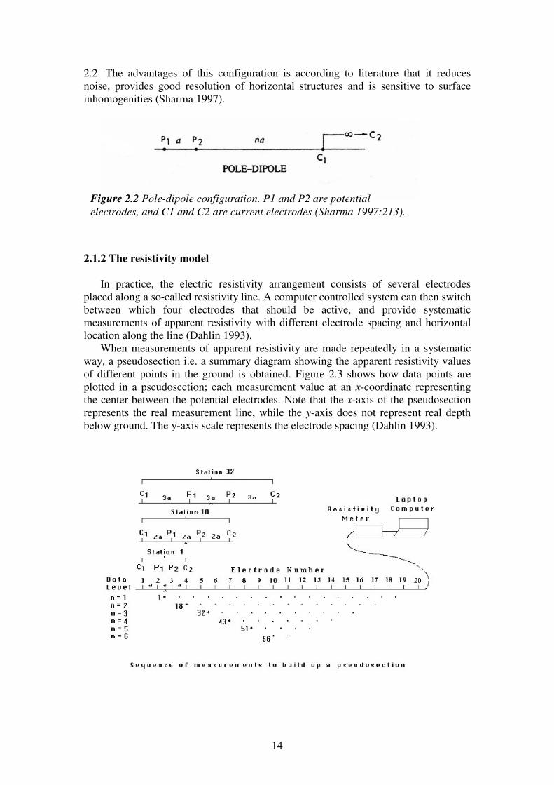
2.1.2 The resistivity model In practice, the electric resistivity arrangement consists of several electrodes

placed along a so-called resistivity line. A computer controlled system can then switch between which four electrodes that should be active, and provide systematic measurements of apparent resistivity with different electrode spacing and horizontal location along the line (Dahlin 1993).

When measurements of apparent resistivity are made repeatedly in a systematic way, a pseudosection i.e. a summary diagram showing the apparent resistivity values of different points in the ground is obtained. Figure 2.3 shows how data points are plotted in a pseudosection; each measurement value at an x-coordinate representing the center between the potential electrodes. Note that the x-axis of the pseudosection represents the real measurement line, while the y-axis does not represent real depth below ground. The y-axis scale represents the electrode spacing (Dahlin 1993).

Figure 2.2 Pole-dipole configuration. P1 and P2 are potential

electrodes, and C1 and C2 are current electrodes (Sharma 1997:213).

15

Apparent resistivity does not represent the reality, since the measured apparent resistivity assumes that the ground is homogeneous. In reality, the ground is often heterogeneous which means that varying materials and objects in the ground contribute in different ways to the measured value of the apparent resistivity. To transform the pseudosection of apparent resistivity values into a soil model with layers and bodies of true resistivity, a computer processing method called inversion is used (Dahlin 1993).

The pseudosection is usually presented as a linearly interpolated contour map, with a color scale representing the differences in apparent resistivity. A computed start model of the ground is set up. The program then calculates a corresponding pseudosection that the computed model with its different layers and bodies of true resistivity would give rise to. During the data inversion, the pseudosection of the computed model of the ground is compared with the measured pseudosection, and the computed ground model is adjusted until both pseudosections agree with each other. When this is achieved, the computed ground model with resistivity values of different subsurface layers and bodies is assumed to represent the reality and can be used for interpretation (Dahlin 1993, Loke 2003).

It is important to realise that different geological models can give rise to the same pseudosection that fits the measured data. There are different techniques for the data inversion, and the best-suited method depends on the site conditions. While some inversion techniques smooths out the boundaries between points of different resistivity (least-squares optimisation method), others keep sharp limits between them (blocky optimisation method). When interpreting the model, it is important to keep in mind that some regions can appear to have too high or low resistivity values because of the data inversion (Loke 2003).

The resistivity values of the ground model are usually placed into cells with fixed sizes and position. The contour maps that are obtained from the inversion program are smoothed out from the inverted data grid, in order to obtain a more realistic picture of the ground. (Jolly et al 2007).

To obtain a 3D-model of the ground, several 2D resistivity profiles are measured and combined (Dahlin 1993).

2.1.3 Resistivity data interpretation

There is a relationship between resistivity and geological material, so ground

measurements of resistivity can be used to determine, for example, if a soil consists of sand, clay or other materials. However, there are other factors that influence the resistivity; high porosity or cracks increases the isolative capacity of the ground, i.e. the resistivity increases. On the other hand, the resistivity decreases with an increasing extent of fluids in the pores of the soil. Also the resistivity of the fluid in the soil pores (mainly determined by salinity), and the mineral composition and the structure of mineral grains affect the resistivity of the ground (Dahlin 1993). Archie’s law is an empirical formula that takes the influence on resistivity of the soil porosity and gas/water fraction in the pores into account:

cb

w fa −− ⋅⋅⋅= φρρ (2.6)

16

where φ is the porosity, f is the fraction of pores containing water and ρw is the resistivity of the pore-water. a, b and c are empirical constants (Keary & Brooks 1991). The values of the constants are dependent on soil type (LaBrecque et al. 1996).

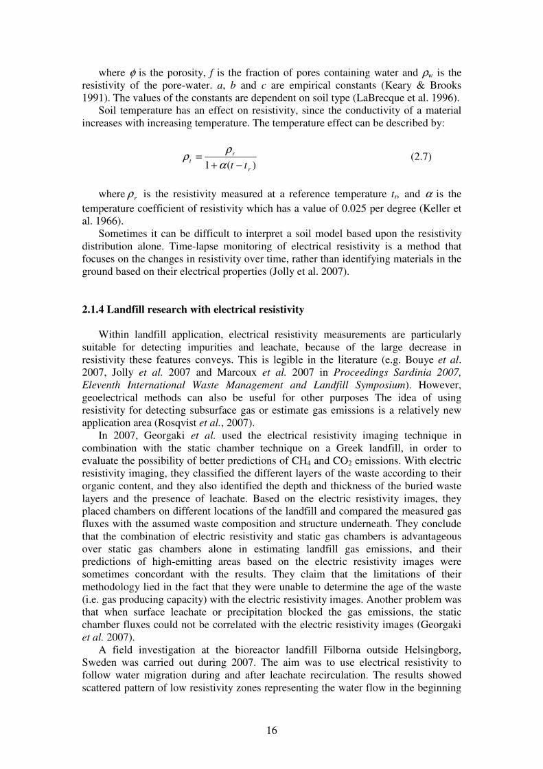
Soil temperature has an effect on resistivity, since the conductivity of a material increases with increasing temperature. The temperature effect can be described by:

)(1 r

rt

tt −+=

α

ρρ (2.7)

where rρ is the resistivity measured at a reference temperature tr, and α is the

temperature coefficient of resistivity which has a value of 0.025 per degree (Keller et al. 1966).

Sometimes it can be difficult to interpret a soil model based upon the resistivity distribution alone. Time-lapse monitoring of electrical resistivity is a method that focuses on the changes in resistivity over time, rather than identifying materials in the ground based on their electrical properties (Jolly et al. 2007).

2.1.4 Landfill research with electrical resistivity

Within landfill application, electrical resistivity measurements are particularly suitable for detecting impurities and leachate, because of the large decrease in resistivity these features conveys. This is legible in the literature (e.g. Bouye et al. 2007, Jolly et al. 2007 and Marcoux et al. 2007 in Proceedings Sardinia 2007,

Eleventh International Waste Management and Landfill Symposium). However, geoelectrical methods can also be useful for other purposes The idea of using resistivity for detecting subsurface gas or estimate gas emissions is a relatively new application area (Rosqvist et al., 2007).

In 2007, Georgaki et al. used the electrical resistivity imaging technique in combination with the static chamber technique on a Greek landfill, in order to evaluate the possibility of better predictions of CH4 and CO2 emissions. With electric resistivity imaging, they classified the different layers of the waste according to their organic content, and they also identified the depth and thickness of the buried waste layers and the presence of leachate. Based on the electric resistivity images, they placed chambers on different locations of the landfill and compared the measured gas fluxes with the assumed waste composition and structure underneath. They conclude that the combination of electric resistivity and static gas chambers is advantageous over static gas chambers alone in estimating landfill gas emissions, and their predictions of high-emitting areas based on the electric resistivity images were sometimes concordant with the results. They claim that the limitations of their methodology lied in the fact that they were unable to determine the age of the waste (i.e. gas producing capacity) with the electric resistivity images. Another problem was that when surface leachate or precipitation blocked the gas emissions, the static chamber fluxes could not be correlated with the electric resistivity images (Georgaki et al. 2007).

A field investigation at the bioreactor landfill Filborna outside Helsingborg, Sweden was carried out during 2007. The aim was to use electrical resistivity to follow water migration during and after leachate recirculation. The results showed scattered pattern of low resistivity zones representing the water flow in the beginning

17

of the irrigation. Eventually, these developed to a more homogeneous zone of low resistivity towards the end of the investigation period. An unexpected result was the irregular zones of increased resistivity at various locations during the experimental period, which were interpreted as possible gas accumulations inside the landfill (Rosqvist et al. 2007).

The idea of identifying high resistivity zones as landfill gas accumulations was also presented by Moreau et al. in 2004. Their investigation site was located at a French bioreactor, where relative changes in resistivity were studied during a leachate recirculation event. In one area of the resistivity profile, the electrical resistivity first decreased, after which it increased before returning to the value it had before the recirculation event. Another point showed the opposite behaviour with an initial rise of resistivity followed by a decrease, before the return to the reference value. The interpretation of this pattern was that a simultaneous flow of liquid and gas in the concerned porous areas could cause the observed variations in resistivity (Moreau et

al. 2004).

2.2 LANDFILL GAS TRANSPORT

2.2.1 Landfill gas

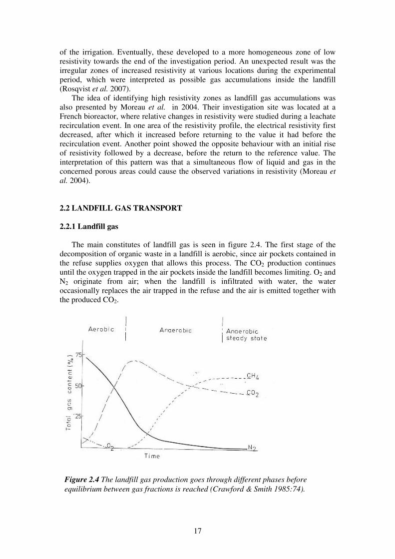
The main constitutes of landfill gas is seen in figure 2.4. The first stage of the decomposition of organic waste in a landfill is aerobic, since air pockets contained in the refuse supplies oxygen that allows this process. The CO2 production continues until the oxygen trapped in the air pockets inside the landfill becomes limiting. O2 and N2 originate from air; when the landfill is infiltrated with water, the water occasionally replaces the air trapped in the refuse and the air is emitted together with the produced CO2.

Figure 2.4 The landfill gas production goes through different phases before

equilibrium between gas fractions is reached (Crawford & Smith 1985:74).

18

When the landfill eventually shifts into its anaerobic phase of gas production, the emission of O2 and N2 declines to nearly zero. Instead the CH4 production starts off and increases as the methanogenic bacteria establish themselves in the landfill, and within 1-2 years after the deposition is the anaerobic steady state reached, i.e. the ratio of CO2 and CH4 respectively is constant. Trace amounts of N2 and H2S are also ambient in landfill gas during the anaerobic phases. An example of the principle of anaerobic decomposition of organic matter is when acetic acid is broken down to CH4 and CO2 (Crawford & Smith 1985):

CH3COOH CH4 + CO2

Factors controlling the production of landfill gas include the waste composition and the age of the refuse. The more organic matter present, the more gas can be produced. After the deposition of the waste it takes some time before microbial organisms reach their optimal efficiency. Furthermore, a large fraction of the available carbon has already been decomposed when the waste has been buried for a long time. The maximum production rate of landfill gas therefore occurs at a time point, where the strain of methanogenic bacteria is established, but organic material is still not limiting (Crawford & Smith 1985).

Physical conditions, mainly temperature and moisture, also affect the gas production. High temperatures and high soil moisture content enhances gas production, as it constitutes a more favourable environment for the microbial organisms (Crawford & Smith 1985).

If oxygen is available in the upper layers of the soil of a CH4 producing landfill, CH4 oxidising bacteria can establish there. These microbial organisms gain energy by the oxidation of CH4, and the result of the reactions is that CH4 is transformed into CO2 (Maurice 1998).

2.2.2 General about gas transport in landfills

There are general theories in the literature about how gas is transported in

landfills. When gas has been produced inside a landfill, it starts to move due to different physical imbalances. Subsurface accumulation of gas causes the gas pressure to rise, which results in pressure differences throughout the landfill. The gas migrates from high pressure to low pressure zones under the soil surface through advection, a process sometimes referred to as pressure flow. (Crawford & Smith 1985). When the gas pressure inside a landfill increases, the gas tends to migrate upwards and outwards to areas of lower pressure (O’Leary & Walsh 2002).

Gas in landfills also moves trough diffusion, a process that derives from gas concentration imbalances between different parts of the landfill. The gas moves from areas of high- to areas of low gas concentration (Crawford & Smith 1985).

In general, gas migrates through the path of least resistance, i.e. the areas of highest permeability (O’Leary & Walsh 2002). The permeability of a soil is related to factors like soil texture, water holding capacity and porosity. Generally, dry soils with large porosity have a higher permeability than moist, fine-grained soils. Cracks and channels in the ground also provide important pathways for gaseous movement (Chapin et al. 2002). Since the construction of landfills is usually made up of packed layers, the gas generally moves in horizontal directions according to Kjeldsen & Fischer (1995).

19

2.2.3 Soil conditions

All soils consist of mineral particles (geological or organic), water and gas. The

relative ratios of these constitutes can be described by the following relationship:

m

b

ρ

ρθαφ −=+= 1 (2.8)

where φ is the total soil porosity, α is the volumetric air content of the pores and θ

is the volumetric water content of the pores. The bulk density ρb is the total density of the dry soil, while ρm represents the density of the mineral soil particles (Chapin 2002, Tang 2003).

Several authors (e.g. Hashemi et al. 2002, Liang et al 2008) have used the ideal gas law to describe the state of gases in the soil pores. If the gas is assumed to be a perfect gas, the relationship between the volume V, the temperature T and the partial pressure pj for a gas substance j is: TRnVp jj ⋅⋅=⋅ (2.9)

where nj is the number of moles and R=8.3143Jmol-1K-1 is the gas constant. If a

gas consists of a mixture of substances, the total gas pressure and number of moles are a sum of the different substances (Campbell 1998). 2.2.3 Soil gas diffusion

Diffusion is a molecular transport process determined by the concentration gradient and a probability coefficient. The transport of gas through diffusion in free air can be described by Fick’s law:

z

CDJ a

∂

∂⋅−= (2.10)

where Da (m2/s) is the diffusion coefficient in air, zC ∂∂ / (kgm-3/m) is the

diffusion gradient, and J is the diffusion flux (kgm-2s-1). The negative sign indicates that the flux is opposite to the concentration gradient (Campbell 1998).

The diffusion coefficient (Da0) for CH4 in air of temperature T0= 273.2K and pressure P0=101.3kPa has a constant value of 0.194cm2/s (Billings et al 2000). Since temperature and pressure determine the mobility of the gas molecules, the value of the diffusion coefficient in air is related to these factors. The dependence of Da on air temperature and air pressure is described by (Tang 2003):

⋅

⋅=

0

75.1

00

P

P

T

TDD aa (2.11)

For diffusion of gas in soils, the path length of the gas in the soil pores and the soil moisture affects the diffusion by acting as obstacles. The value of the diffusion

20

coefficient in soils is therefore an estimated fraction of the diffusion coefficient of the air:

as DD ⋅= τ (2.12)

where τ is the tortuosity factor which takes the air filled porosity α and the ratio of the actual path length in the soil to the free path length in air into account (Visscher et. Al 2003, Jassal 2005).

There are different emphirical relationships for τ in the literature, depending on the soil properties where it is applied. Visscher et al. used the following relation in their study of CH4 diffusion in repacked landfill soils (Visscher et. Al 2003):

φ

ατ

5,2

= (2.13)

2.3 Soil gas advection

The advection transport process involves movements of whole air packages in contrast to molecular transport. Gas flow due to pressure differences can be estimated with Darcy’s law, which describes the flow velocity (m3m-2s-1) of a fluid over a pressure gradient in a porous media:

z

PkQ

∂

∂⋅−=

µ (2.14)

where k(m2) is the intrinsic permeability of the media, µ(kgm-1s-1) is the viscosity

of the fluid and zP ∂∂ / (Nm-2/m) is the pressure gradient (Stepniewski 2002, Barber 1990). The intrinsic permeability is a constant for a given medium material or pore structure (Moon et. Al 2008).

A number of authors have used Darcy’s law when modeling landfill gas advection in soils (e.g. Barber et al 1990, Moon et al. 2008, Sanchez et al 2006). Choi et al. (2002) used the following version of Darcy’s law when modeling gas advection in an unsaturated soil:

z

PkQ

∂

∂⋅

⋅−=

αµ (2.15)

where α is the volumetric air content, which origins in an adjustment of the flow

velocity in equation (2.13) to the actual amount of gas in the medium. In other words, α is used as a supplement variable to the intrinsic permeability µ for describing the pore structure of the media (Choi et al. 2002).

21

3 EXPERIMENTAL METHODS & MATERIALS 3.1 SITE DESCRIPTION & MEASUREMENT PERIOD

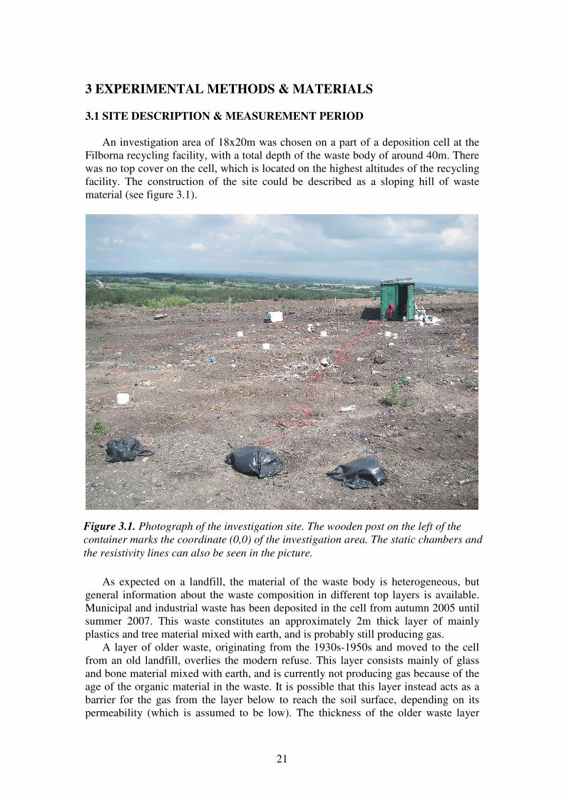
An investigation area of 18x20m was chosen on a part of a deposition cell at the Filborna recycling facility, with a total depth of the waste body of around 40m. There was no top cover on the cell, which is located on the highest altitudes of the recycling facility. The construction of the site could be described as a sloping hill of waste material (see figure 3.1).

As expected on a landfill, the material of the waste body is heterogeneous, but general information about the waste composition in different top layers is available. Municipal and industrial waste has been deposited in the cell from autumn 2005 until summer 2007. This waste constitutes an approximately 2m thick layer of mainly plastics and tree material mixed with earth, and is probably still producing gas.

A layer of older waste, originating from the 1930s-1950s and moved to the cell from an old landfill, overlies the modern refuse. This layer consists mainly of glass and bone material mixed with earth, and is currently not producing gas because of the age of the organic material in the waste. It is possible that this layer instead acts as a barrier for the gas from the layer below to reach the soil surface, depending on its permeability (which is assumed to be low). The thickness of the older waste layer

Figure 3.1. Photograph of the investigation site. The wooden post on the left of the

container marks the coordinate (0,0) of the investigation area. The static chambers and

the resistivity lines can also be seen in the picture.

22

varies between 0-0.5m, which means that the modern waste reaches the soil surface at irregular places around the investigation site.

The composition of the waste below 3m is unknown, but also irrelevant to this investigation since it focuses on the upper layers of the soil. In addition to this general structure of the deposition cell, there is also a body of compost material running through the whole investigation area around the coordinates x=17m. The compost body consist of earth and wood chips and is relatively porous, and the body gets thicker with depth below the soil surface.

In the vicinity of x=17m, there is also a horizontal gas pipe running through the investigation area at a depth of 1m. At approximately x=17m and y=18m, there is a gas well connected to this pipe (see figure 3.2 below). In connection to the well is a porous sand layer.

Although the field measurements of the project as a whole continued for several months (24th of June –2nd of September 2008), the period of interest for this thesis consisted of mainly one week in August (18th-22nd) and partly one week in July (4th-11th). During these two weeks, static chamber measurements of CH4 emissions from the surface were performed. However, since resistivity data is missing from the week in July, the main focus is put on the period in August. 3.2 ELECTRICAL RESISTIVITY SETUP

The ABEM Lund Imaging System was used for the resistivity measurements,

which is a computer-controlled system for electrode relay-switching, current transmission and data acquisition. The instrumental arrangement consisted of nine lines of electrodes, with a distance of 2m between each pair of lines (see figure 3.1). The electrode spacing was 1m; i.e. a total number of 21 electrodes per line. All electrodes in each line were connected to a cable (with internal cables for each electrode), which in turn were connected to a switching unit (three ES464 switching units were necessary for this arrangement). The switching units were automatically controlled by a computer, which means that the system could connect or disconnect each of the nine lines to the measurement instrument. The measurement instrument controlled which electrodes in the active line that were used to send current through or measure potential between.

The electrode configuration pol-dipol was used to obtain deeper ground penetration, which means that the current was sent between a distant electrode (here ca 100m away from the measurement area) and an electrode in the active resistivity line, when a measurement was done. Since the instrument has seven measurement channels, it was possible to use different combinations of seven electrodes (in the active line) as potential electrodes during each measurement, which makes the measurements more time-effective.

The data was collected in files and sent to Lund via Internet, and the pseudosections were inverted with the program Res3Dinv (Geotemo Software SDN. BHD). The inversion method used was the so-called robust inversion, which uses equal weights of the measurement points when calculating the soil model, and reduces the risk of artefacts in the data (Leroux, personal communication. For a more detailed description of the resistivity experimental setup, I reefer to the project report).

23

3.3 SURFACE CH4 FLUX 3.3.1 Static gas chamber measurements

The principal idea of static gas chamber measurements is to measure how the concentration of a specific gas rises inside a chamber, placed upon a gas-emitting surface.

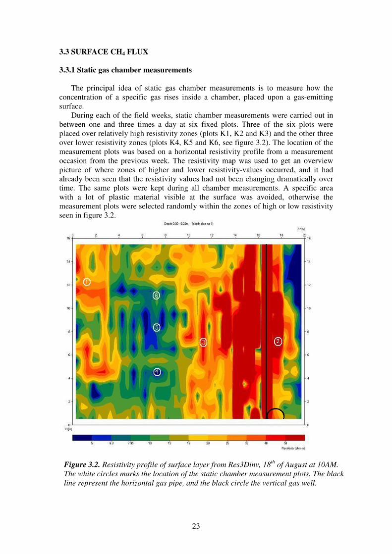
During each of the field weeks, static chamber measurements were carried out in between one and three times a day at six fixed plots. Three of the six plots were placed over relatively high resistivity zones (plots K1, K2 and K3) and the other three over lower resistivity zones (plots K4, K5 and K6, see figure 3.2). The location of the measurement plots was based on a horizontal resistivity profile from a measurement occasion from the previous week. The resistivity map was used to get an overview picture of where zones of higher and lower resistivity-values occurred, and it had already been seen that the resistivity values had not been changing dramatically over time. The same plots were kept during all chamber measurements. A specific area with a lot of plastic material visible at the surface was avoided, otherwise the measurement plots were selected randomly within the zones of high or low resistivity seen in figure 3.2.

Figure 3.2. Resistivity profile of surface layer from Res3Dinv, 18th

of August at 10AM.

The white circles marks the location of the static chamber measurement plots. The black

line represent the horizontal gas pipe, and the black circle the vertical gas well.

24

The heterogeneous structure of the landfill surface resulted in the fact that the

cover material of the plots differed. The visible surface material at plots K1 and K6 consisted mainly of wood chips, while the surface of plot K5 consisted of relatively much sand and clay. At plots K2, K3 and K4 the cover material seemed to be humus rich sandy soil.

Upside-down buckets with a volume of 12dm3 were used as static chambers, and septum sealed openings for air sampling were placed on the top (see figure 3.3). Every time the chambers where placed on the ground, they were sealed for air leakage with wet clay, since there were no possibility to use other solutions for sealing the chamber to the ground surface.

Once the chambers were placed on the ground and sealed with clay, a 20 ml gas sample was collected with a syringe and saved in a 10 ml glass vial. After 10 and 20 minutes respectively, the gas sampling was repeated to complete the measurement series of one single flux measurement.

3.3.2 Lab analysis and flux calculations

The air samples were separated by gas chromatography (GC, Shimadzu 17A) and detected by flame ionization detection (FID). Injection/detection and column oven tempertures were 140 °C and 70 °C, respectively. The samples were introduced into the GC column (Porapak Q) by syringe injection via a 1 ml sample loop. Helium was used as carrier gas with a flow rate of 40 ml min-1. In the GC column, CH4 molecules are separated from other gas constituents, whereafter it is pyrolysed in the hydrogen

Figure 3.3. The static chambers were sealed for air leakage with wet clay,

and samples were taken through a septum sealed opening. Soil temperature

was measured with an all-round thermometer.

25

flame of the FID-detector. The resulting ions and electrones gives rise to a current, i.e. a peak in voltage, which’s size is proportional to the mixing ratio of the gas in the sample. During the GC-analysis it is therefore necessary to use gas standards; that is injection of gas with a known CH4 mixing ratio, to set up a relation between peak area and mixing ratio. Since the gas samples were kept in glass vials for several months in between the fieldwork and the GC-analysis, CH4 standards were also kept in glass vials together with the samples in order to estimate and correct for the possible leakage from the vials during this period of time. In addition were blank samples of background air collected from the time point when the vials were closed in the lab. During the flux calculations, they were used to correct for the ambient atmospheric CH4 present in the vials.

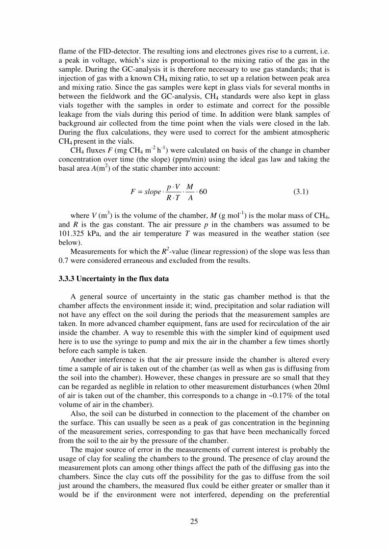
CH4 fluxes F (mg CH4 m-2 h-1) were calculated on basis of the change in chamber

concentration over time (the slope) (ppm/min) using the ideal gas law and taking the basal area A(m2) of the static chamber into account:

60⋅⋅⋅

⋅⋅=

A

M

TR

VpslopeF (3.1)

where V (m3) is the volume of the chamber, M (g mol-1) is the molar mass of CH4,

and R is the gas constant. The air pressure p in the chambers was assumed to be 101.325 kPa, and the air temperature T was measured in the weather station (see below).

Measurements for which the R2-value (linear regression) of the slope was less than 0.7 were considered erraneous and excluded from the results. 3.3.3 Uncertainty in the flux data

A general source of uncertainty in the static gas chamber method is that the

chamber affects the environment inside it; wind, precipitation and solar radiation will not have any effect on the soil during the periods that the measurement samples are taken. In more advanced chamber equipment, fans are used for recirculation of the air inside the chamber. A way to resemble this with the simpler kind of equipment used here is to use the syringe to pump and mix the air in the chamber a few times shortly before each sample is taken.

Another interference is that the air pressure inside the chamber is altered every time a sample of air is taken out of the chamber (as well as when gas is diffusing from the soil into the chamber). However, these changes in pressure are so small that they can be regarded as neglible in relation to other measurement disturbances (when 20ml of air is taken out of the chamber, this corresponds to a change in ~0.17% of the total volume of air in the chamber).

Also, the soil can be disturbed in connection to the placement of the chamber on the surface. This can usually be seen as a peak of gas concentration in the beginning of the measurement series, corresponding to gas that have been mechanically forced from the soil to the air by the pressure of the chamber.

The major source of error in the measurements of current interest is probably the usage of clay for sealing the chambers to the ground. The presence of clay around the measurement plots can among other things affect the path of the diffusing gas into the chambers. Since the clay cuts off the possibility for the gas to diffuse from the soil just around the chambers, the measured flux could be either greater or smaller than it would be if the environment were not interfered, depending on the preferential

26

pathways of the gas in the soil at the specific location. This problem increased during the field periods, since the remaining layer of clay around the plots became harder to remove after each measurement, especially after rain events.

Finally, it is also possible that there has been air leakage from the chambers during some of the measurements, since the clay may not always have sealed the chambers to the ground perfectly.

3.4 ENVIRONMENTAL VARIABLES

3.4.1 Soil temperature

Simultaneously with each static chamber measurement, weather station

independent soil temperature measurements were done with a simple all-round thermometer in the vicinity of the chamber (see figure 3.3).

3.4.2 Soil moisture

Twelve TDR-probes were installed in the ground, equally spaced over a larger

part of the investigation area (see figure 3.4). The probes were 30cm long, which means that the measured soil moisture

represent the average soil moisture in the upper 30cm of the soil. The probes were via cables connected to a multiplexer and a TDR100-instrument, which were controlled manually from a computer. A waveform appeared as a result when a measurement was made on a certain probe. The wavelength of the waveform is dependent on the electric permittivity of the soil, which in turn is dependent on soil moisture. The waveforms were later recalculated to relative estimates of soil moisture The soil moisture values are unfortunately probably rather uncertain, mainly because no soil samples were taken at the site to be used for calibration of the TDR-probes (Leroux pers. comm). However, the measurements are still useful for analysing the relative changes of the soil moisture during the week. Measurements were carried out about three times per day ((Leroux, Månsson personal comments).

27

3.4.3 Weather station

A weather station with a Campbell C1000 data logger (Campbell Manufactoring) was installed at the investigation area. Air pressure (Setra 278), wind speed and wind direction (Wind Sonic, 1 m above the ground surface), air temperature (1 m above the ground surface), soil temperature (5 cm into the ground) and precipitation (ARG10, tipping bucket) were recorded every second, and averaged to one-minute values. The weather station logger sometimes underestimated the amount of precipitation, but it should be reliable that all rain events were at least recorded at the right time points (Lindsjö personal comment).

The data set was later extrapolated to half-hourly averages using a running average (precipitation summarized for every half-hour).

A1

B1

C1

D1

A2

B2

C2

D2

A3

B3

C3

D3

B4

C4 C5

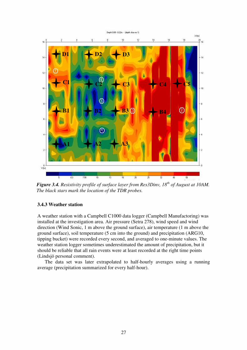
Figure 3.4. Resistivity profile of surface layer from Res3Dinv, 18th

of August at 10AM.

The black stars mark the location of the TDR probes.

28

4. DATA ANALYSIS METHODS 4.1 TIME-LAPS ANALYSIS OF RESISTIVITY DATA

The inverted resistivity data consisted of 640 coordinate values for each horizontal

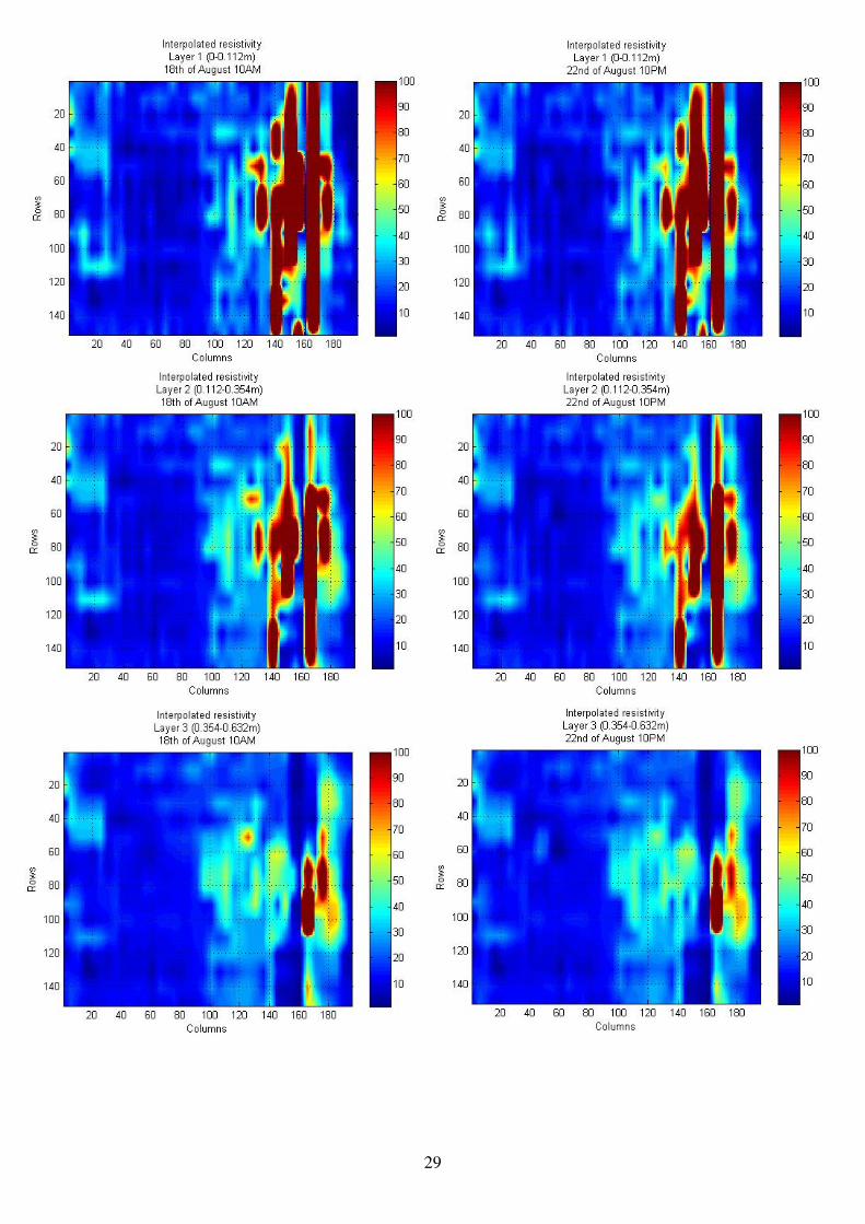
resistivity profile (in total 17 layers). The coordinates for the six upper layers were imported and handled as matrices in Matlab. Each rectangular cell in the original data files corresponds to an area of 0.5m x 1m of the soil. The difference in resistivity between neighbouring cells is often large. The data values were linearly interpolated in order to smooth out these rough borders between the cells, and to improve a spatial analysis. Each cell in the interpolated model corresponds to 0.1m x 0.1m area of the soil.

Since the aim of this thesis is to look at soil gas behaviour and gas transport, it is important to focus on the changes in resistivity over time. In earlier research, it has been shown clearly that water migration in landfills is well detected as a decrease in resistivity. It is therefore convenient to assume that an increase in resistivity on the other hand can be a result of the behaviour of the gas in the landfill (Rosqvist et al 2007). Looking at the changes in resistivity rather than the resistivity values alone reduces the risk of interpreting high resistivity materials in the ground as gas.

It was early noticed from a visual interpretation, that areas of high resistivity values oscillated, grew larger and smaller in a way that reminded of a periodic behaviour. Any horizontal movements of gas, that theoretically is common in landfill, could not be seen.

A complete set of resistivity data took around two hours to measure. Two-hourly data from 10AM on the 18th of August to 22 PM on the 22nd of August was used in the analysis.

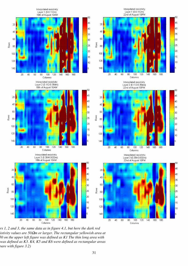
Areas in the ground underneath the measurement plots K1-K6 were identified in the resistivity matrices, and the average resistivity values of each horizontal layer in the areas were calculated and plotted on a time axis. Underneath measurement plots K1, K2 and K3 an attempt to identify presumed gas assimilations was made through setting a mimimum value for the data cells in the matrix to be included in the plot area (see figures 4.1 and 4.2). To look at the behavior of gas assimilations underneath the chambers, rather than a more limited random area, was believed to improve the possibilities of finding relationships between soil gas behavior and surface emissions.

The resistivity values underneath measurement plots K4, K5 and K6 were very low over a large area with no steep changes in resistivity. For analysing the resistivity changes underneath these plots, rectangular areas corresponding to 0.33 m2 of the soil surrounding the chambers were selected (the basal area of the static chambers was 0.06m2). With the number of cells included in the each plot area selected kept constant over the week, the variations in resistivity over time is likely to reflect the changes of the soil state during the week.

31

Resistivity maps of layers 1, 2 and 3, the same data as in figure 4.1, but here the dark red

color represent areas where the resistivity values are 50Ωm or larger. The rectangular yellowish area at approximately column 20 and row 50 on the upper left figure was defined as K1 The thin long area with

a center at column 110 and row 80 was defined as K3. K4, K5 and K6 were defined as rectangular areas

with centers along column 60 (compare with figure 3.2)

32

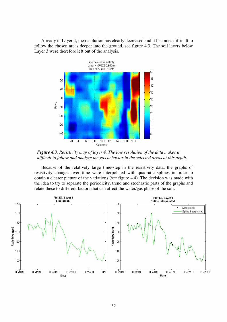
Already in Layer 4, the resolution has clearly decreased and it becomes difficult to follow the chosen areas deeper into the ground, see figure 4.3. The soil layers below Layer 3 were therefore left out of the analysis.

Because of the relatively large time-step in the resistivity data, the graphs of resistivity changes over time were interpolated with quadratic splines in order to obtain a clearer picture of the variations (see figure 4.4). The decision was made with the idea to try to separate the periodicity, trend and stochastic parts of the graphs and relate these to different factors that can affect the water/gas phase of the soil.

Figure 4.3. Resistivity map of layer 4. The low resolution of the data makes it

difficult to follow and analyze the gas behavior in the selected areas at this depth.

33

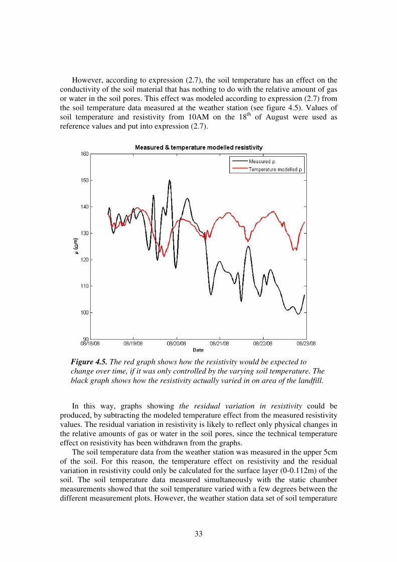
However, according to expression (2.7), the soil temperature has an effect on the

conductivity of the soil material that has nothing to do with the relative amount of gas or water in the soil pores. This effect was modeled according to expression (2.7) from the soil temperature data measured at the weather station (see figure 4.5). Values of soil temperature and resistivity from 10AM on the 18th of August were used as reference values and put into expression (2.7).

In this way, graphs showing the residual variation in resistivity could be

produced, by subtracting the modeled temperature effect from the measured resistivity values. The residual variation in resistivity is likely to reflect only physical changes in the relative amounts of gas or water in the soil pores, since the technical temperature effect on resistivity has been withdrawn from the graphs.

The soil temperature data from the weather station was measured in the upper 5cm of the soil. For this reason, the temperature effect on resistivity and the residual variation in resistivity could only be calculated for the surface layer (0-0.112m) of the soil. The soil temperature data measured simultaneously with the static chamber measurements showed that the soil temperature varied with a few degrees between the different measurement plots. However, the weather station data set of soil temperature

Figure 4.5. The red graph shows how the resistivity would be expected to

change over time, if it was only controlled by the varying soil temperature. The

black graph shows how the resistivity actually varied in on area of the landfill.

34

was used for all measurement plots when calculating the residual variation in resistivity, since this was the only sufficient data set available.

This methodological approach leads to the assumption that the main changes of

resistivity in the ground correspond to a change in the gas-water phase of the soil

pores. Since a week is a relatively short period of investigation, settlement of the landfill and other possible causes of physical changes in the ground can be neglected.

4.2 VARIATIONS IN SURFACE CH4 FLUXES

The CH4 flux data was analysed with a number of statistical test; the Kolmogorov-

Smirnov test for normality, the One-way ANOVA (Analysis of Variance) test for significant differences between mean values of the measurement plots, and a post-hoc One-way ANOVA Bonferroni test that, after general significance had been achieved, was used to analyse which individual measurement plots that were significantly different. 4.3 SOIL GAS DIFFUSION AND ADVECTION

The diffusion coefficient in free air, Da, was estimated from the recorded soil temperature and air pressure data, using expression (2.10). The values of Da were together with the values of the soil moisture measured in field put into expression (2.11) and (2.12) above to obtain values for the soil diffusion coefficient. Since no soil samples were made; the value for soil porosity (0.6) had to be approximated for the calculations. The modelled soil diffusion coefficient shows therefore relative changes over the week due to the variations in temperature, pressure and soil moisture.

In order to model soil diffusion and advection and compare these with measured fluxes, measurement of soil concentration and pressure would be necessary. Since no such measurements were performed in the field, the expressions (2.9) and (2.14) will mainly be useful for understanding how the environmental variables affect the different transport processes, and theoretically relate these to the measured CH4

fluxes.

‘

35

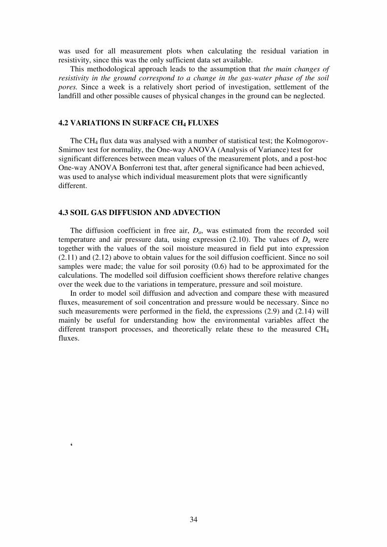
5. RESULTS 5.1 VARIATION IN CH4 FLUXES

The measured CH4 fluxes showed a large variation in all six plots, at several

measurement plots, many of them were negative. According to the statistical tests, the fluxes from plots K2 and K3 were significantly different from the rest of the plots (F-value 13.766, p-value <0.03 for K2 and p-value <0.001 for K3). These were the two plots where the highest CH4 fluxes were measured, and they were with only a few exceptions always positive. Table 5.1 and 5.2 below summarize the resulting fluxes measured in July and August, respectively. In general, the fluxes were at all plots higher in July than in August.

July K1 K2 K3 K4 K5 K6

Max flux

(mg/m2/h) 5.89 1048.82 1550.14 5.63 55.33 15.09

Min flux (mg/m

2/h) -2.42 35.00 16.13 -42.78 1.13 -4.77

Mean flux

(mg/m2/h) 1.71 390.27 683.13 -16.50 22.80 3.28

Median flux

(mg/m2/h) 0.76 302.94 776.40 -18.07 9.08 1.78

August K1 K2 K3 K4 K5 K6

Max flux

(mg/m2/h) 1.49 513.66 994.61 11.44 6.39 5.31

Min flux (mg/m

2/h) -2.88 1.45 -13.36 -50.76 -5.37 -7.75

Mean flux

(mg/m2/h) -1.30 258.08 385.00 -11.37 0.67 -0.50

Median flux

(mg/m2/h) -1.53 276.11 407.46 -8.67 0.84 -0.51

The fluxes showed signs of correlatation with soil temperature, air temperature, air pressure and soil moisture, but due to the undefined nature of the substrate directly underlying the chambers it was not considered meaningful to pursue a rigorous statistical analysis. In addition, there was no clear correlation between the resistivity values in the ground below the measurement plots and the size of the CH4 fluxes.

Table 5.1. Summary of CH4 flux results from July

Table 5.2. Summary of CH4 flux results from August

36

5.2 CH4 FLUXES AND VARIATIONS IN RESISTIVITY

5.2.1 Plot K1

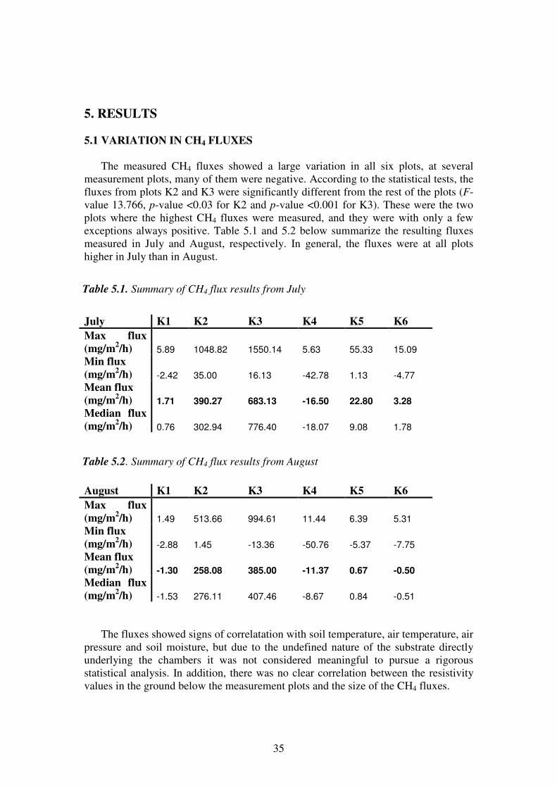
The variations in resistivity of the three upper layers (Layer 1 at 0.112m, Layer 2

at 0.354m and Layer 3 at 0.632m) in the ground below plot K1 was, together with the CH4 fluxes, plotted against time in figure 5.1. The actual resistivity values here ranged between ~28-33Ωm during the week; i.e. this was not an area of particularly high resistivity. Figure 5.1 shows the variation in resistivity below plot K1. As can be seen, the resistivity values and variations are very similar in the three upper layers of the soil. However, it is difficult to see any patterns and to analyse what causes these variations.

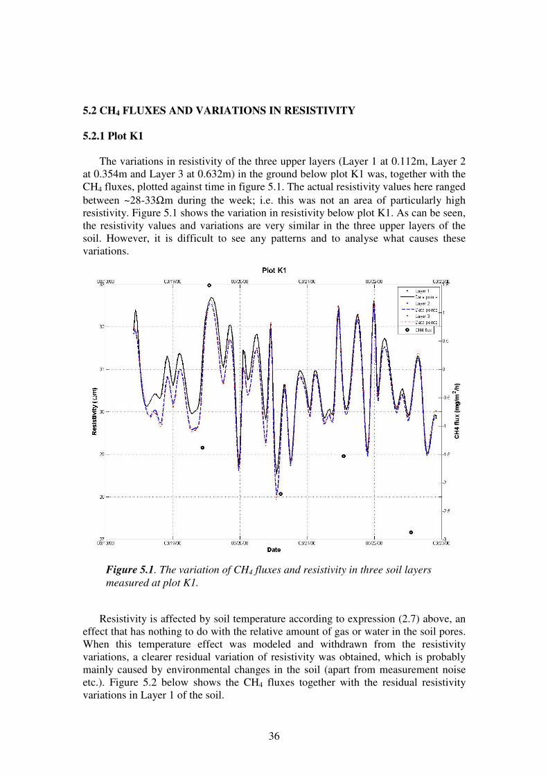
Resistivity is affected by soil temperature according to expression (2.7) above, an

effect that has nothing to do with the relative amount of gas or water in the soil pores. When this temperature effect was modeled and withdrawn from the resistivity variations, a clearer residual variation of resistivity was obtained, which is probably mainly caused by environmental changes in the soil (apart from measurement noise etc.). Figure 5.2 below shows the CH4 fluxes together with the residual resistivity variations in Layer 1 of the soil.

Figure 5.1. The variation of CH4 fluxes and resistivity in three soil layers

measured at plot K1.

37

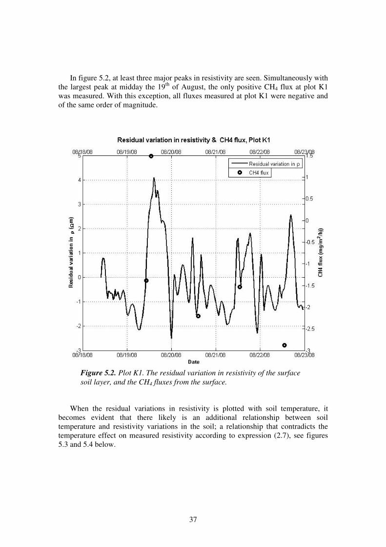
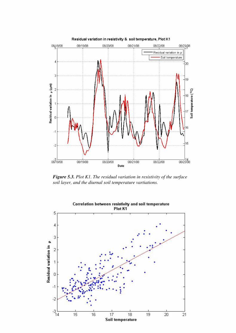
In figure 5.2, at least three major peaks in resistivity are seen. Simultaneously with

the largest peak at midday the 19th of August, the only positive CH4 flux at plot K1 was measured. With this exception, all fluxes measured at plot K1 were negative and of the same order of magnitude.

When the residual variations in resistivity is plotted with soil temperature, it becomes evident that there likely is an additional relationship between soil temperature and resistivity variations in the soil; a relationship that contradicts the temperature effect on measured resistivity according to expression (2.7), see figures 5.3 and 5.4 below.

Figure 5.2. Plot K1. The residual variation in resistivity of the surface

soil layer, and the CH4 fluxes from the surface.

38

Figure 5.3. The residual resistivity resistivity variation in Layer 1 and

soil temperature at plot K1.


soil layer, and the diurnal soil temperature vartiations.

39

5.2.2 Plot K2

Figure 5.5 below represents plots of the resistivity variations in soil layers 1, 2 and

3together with CH4 fluxes. Plot K2 is located above a zone of particulary high resistivity values, possibly a soil gas pocket, which ranges from ~100-150Ωm in Layer 1. As seen in figure 5.5, the resistivity is generally higher in Layer 2 than in Layer 1, but the variations in these layers follow each other well. However, in Layer 3 the variations look different, and sometimes even opposite to the upper soil (e.g. the negative peaks in Layer 1 and 2 and the simultaneously positive peak in Layer 3 around midnight at the 19th of August).

In figure 5.5, it is vaguely possible to see the technical soil temperature effect on

the resistivity in Layer 1 and 2 as periodic behavior, inversely proportional to the soil temperature variations that have a maximum around midday and minimum early in the morning. Figure 5.6 below shows the residual variation in resistivity together with CH4 fluxes, and comparing figure 5.5 and 5.6 stress how this approach helps to sort out physical changes in the soil from other effects.

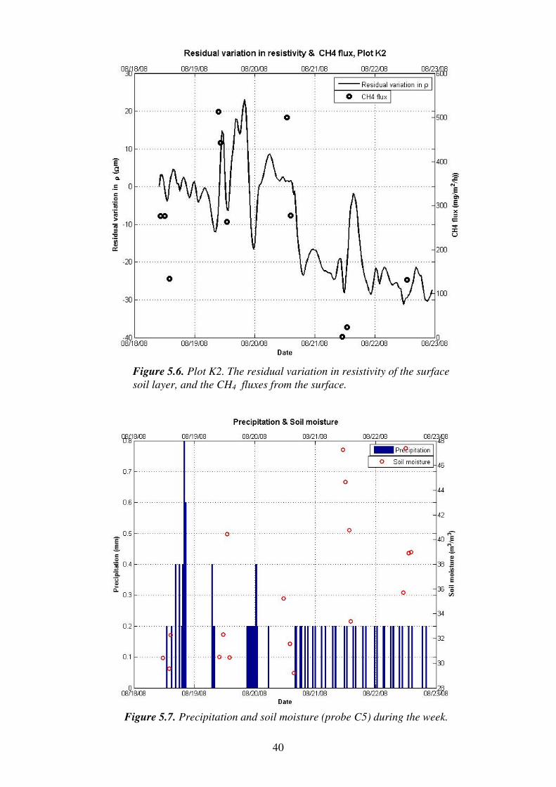
In figure 5.6, three major resistivity peaks and a clearly decreasing trend of resistivity during the week are seen. Figure 5.7 below shows the precipitation and the soil moisture measured during the week.

Figure 5.4. Correlation between normalized resistivity variation in Layer

1 and soil temperature at plot K1.



Figure 5.4. Correlation between the soil temperature and the residual

variation in resistivity.

40

Figure 5.7. Precipitation and soil moisture (probe C5) during the week.



41

Comparing figure 5.6 and 5.7, it is evident that increasing soil moisture during the week is very likely to cause the decreasing trend of resistivity. There is also an indication that the CH4 fluxes decrease with increasing soil moisture. Another interesting observation is that the two large rain events during the 19th of August result in simultaneous negative peaks in resistivity. In both cases, the resistivity shortly after rises to considerable positive peaks, and the CH4 fluxes reaches maximum values.

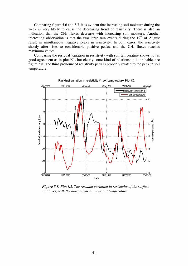
Comparing the residual variation in resistivity with soil temperature shows not as good agreement as in plot K1, but clearly some kind of relationship is probable, see figure 5.8. The third pronounced resistivity peak is probably related to the peak in soil temperature.


soil layer, with the diurnal variation in soil temperature.

42

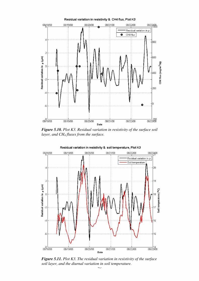
5.2.3 Plot K3

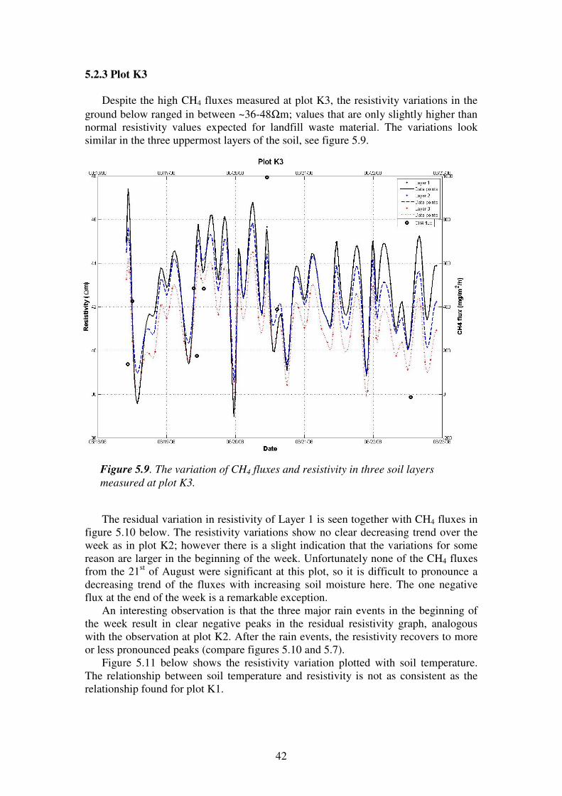
Despite the high CH4 fluxes measured at plot K3, the resistivity variations in the

ground below ranged in between ~36-48Ωm; values that are only slightly higher than normal resistivity values expected for landfill waste material. The variations look similar in the three uppermost layers of the soil, see figure 5.9.

The residual variation in resistivity of Layer 1 is seen together with CH4 fluxes in

figure 5.10 below. The resistivity variations show no clear decreasing trend over the week as in plot K2; however there is a slight indication that the variations for some reason are larger in the beginning of the week. Unfortunately none of the CH4 fluxes from the 21st of August were significant at this plot, so it is difficult to pronounce a decreasing trend of the fluxes with increasing soil moisture here. The one negative flux at the end of the week is a remarkable exception.

An interesting observation is that the three major rain events in the beginning of the week result in clear negative peaks in the residual resistivity graph, analogous with the observation at plot K2. After the rain events, the resistivity recovers to more or less pronounced peaks (compare figures 5.10 and 5.7).

Figure 5.11 below shows the resistivity variation plotted with soil temperature. The relationship between soil temperature and resistivity is not as consistent as the relationship found for plot K1.



43

Figure 5.10. Plot K3. Residual variation in resistivity of the surface soil

layer, and CH4 fluxes from the surface.


soil layer, and the diurnal variation in soil temperature.

44

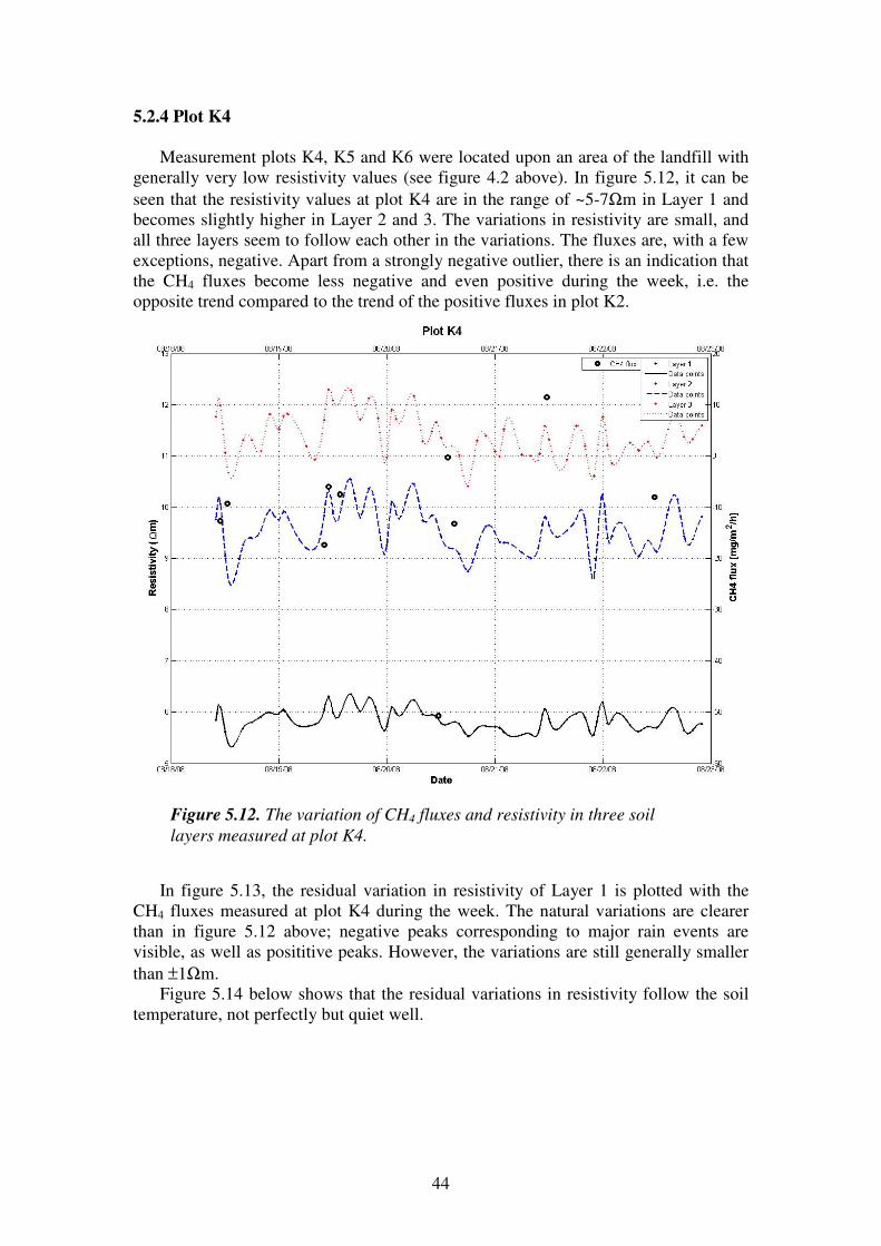
5.2.4 Plot K4

Measurement plots K4, K5 and K6 were located upon an area of the landfill with

generally very low resistivity values (see figure 4.2 above). In figure 5.12, it can be seen that the resistivity values at plot K4 are in the range of ~5-7Ωm in Layer 1 and becomes slightly higher in Layer 2 and 3. The variations in resistivity are small, and all three layers seem to follow each other in the variations. The fluxes are, with a few exceptions, negative. Apart from a strongly negative outlier, there is an indication that the CH4 fluxes become less negative and even positive during the week, i.e. the opposite trend compared to the trend of the positive fluxes in plot K2.

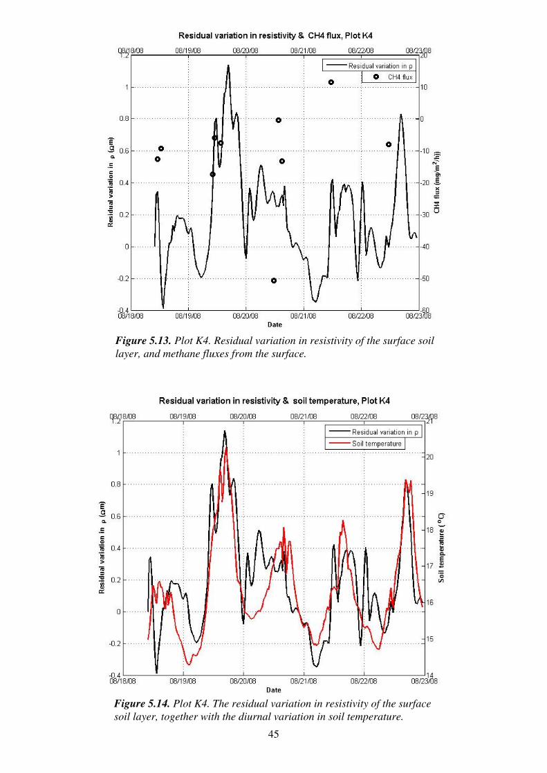
In figure 5.13, the residual variation in resistivity of Layer 1 is plotted with the

CH4 fluxes measured at plot K4 during the week. The natural variations are clearer than in figure 5.12 above; negative peaks corresponding to major rain events are visible, as well as posititive peaks. However, the variations are still generally smaller than ±1Ωm.

Figure 5.14 below shows that the residual variations in resistivity follow the soil temperature, not perfectly but quiet well.

Figure 5.12. The variation of CH4 fluxes and resistivity in three soil

layers measured at plot K4.

45

Figure 5.13. Plot K4. Residual variation in resistivity of the surface soil

layer, and methane fluxes from the surface.


soil layer, together with the diurnal variation in soil temperature.

46

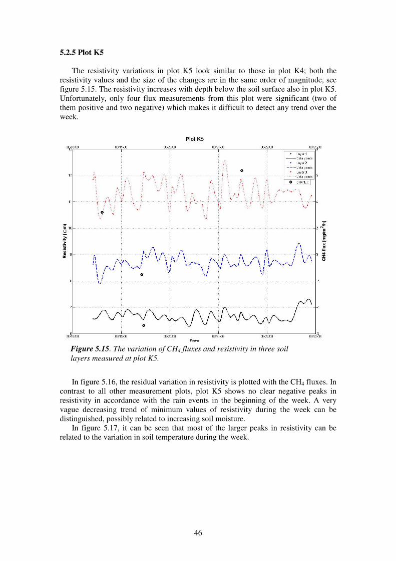
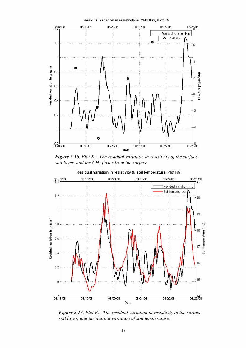
5.2.5 Plot K5

The resistivity variations in plot K5 look similar to those in plot K4; both the

resistivity values and the size of the changes are in the same order of magnitude, see figure 5.15. The resistivity increases with depth below the soil surface also in plot K5. Unfortunately, only four flux measurements from this plot were significant (two of them positive and two negative) which makes it difficult to detect any trend over the week.

In figure 5.16, the residual variation in resistivity is plotted with the CH4 fluxes. In contrast to all other measurement plots, plot K5 shows no clear negative peaks in resistivity in accordance with the rain events in the beginning of the week. A very vague decreasing trend of minimum values of resistivity during the week can be distinguished, possibly related to increasing soil moisture.

In figure 5.17, it can be seen that most of the larger peaks in resistivity can be related to the variation in soil temperature during the week.

Figure 5.15. The variation of CH4 fluxes and resistivity in three soil


47




soil layer, and the diurnal variation of soil temperature.

48

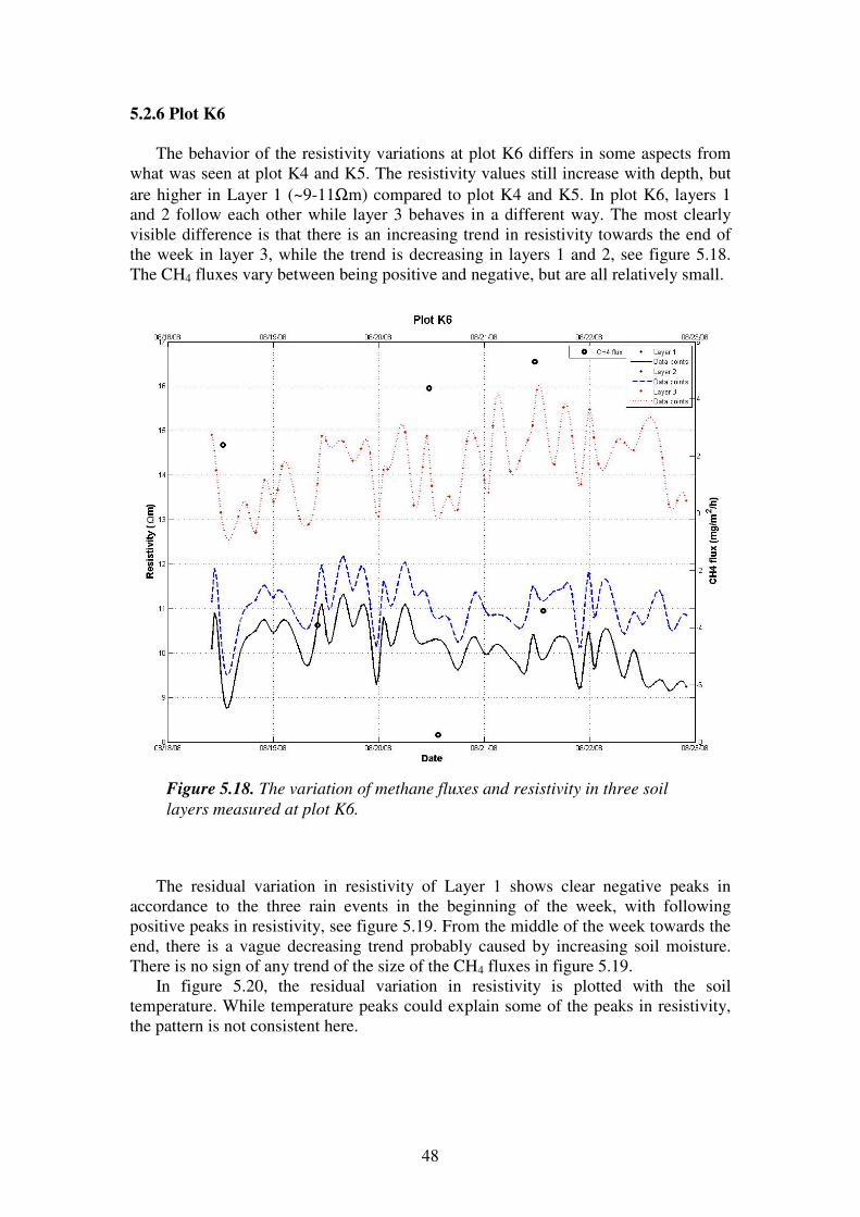
5.2.6 Plot K6

The behavior of the resistivity variations at plot K6 differs in some aspects from

what was seen at plot K4 and K5. The resistivity values still increase with depth, but are higher in Layer 1 (~9-11Ωm) compared to plot K4 and K5. In plot K6, layers 1 and 2 follow each other while layer 3 behaves in a different way. The most clearly visible difference is that there is an increasing trend in resistivity towards the end of the week in layer 3, while the trend is decreasing in layers 1 and 2, see figure 5.18. The CH4 fluxes vary between being positive and negative, but are all relatively small.

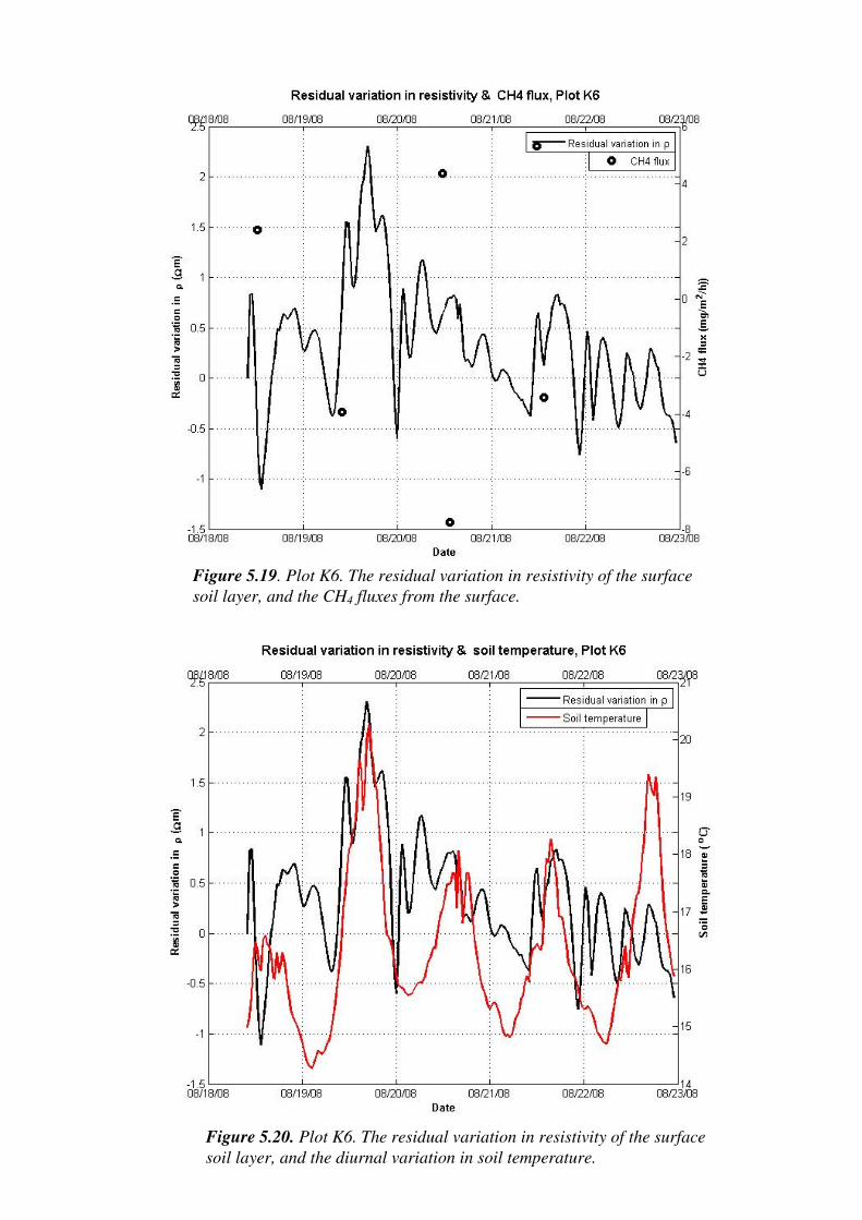
The residual variation in resistivity of Layer 1 shows clear negative peaks in

accordance to the three rain events in the beginning of the week, with following positive peaks in resistivity, see figure 5.19. From the middle of the week towards the end, there is a vague decreasing trend probably caused by increasing soil moisture. There is no sign of any trend of the size of the CH4 fluxes in figure 5.19.

In figure 5.20, the residual variation in resistivity is plotted with the soil temperature. While temperature peaks could explain some of the peaks in resistivity, the pattern is not consistent here.

Figure 5.18. The variation of methane fluxes and resistivity in three soil


49




soil layer, and the diurnal variation in soil temperature.

50

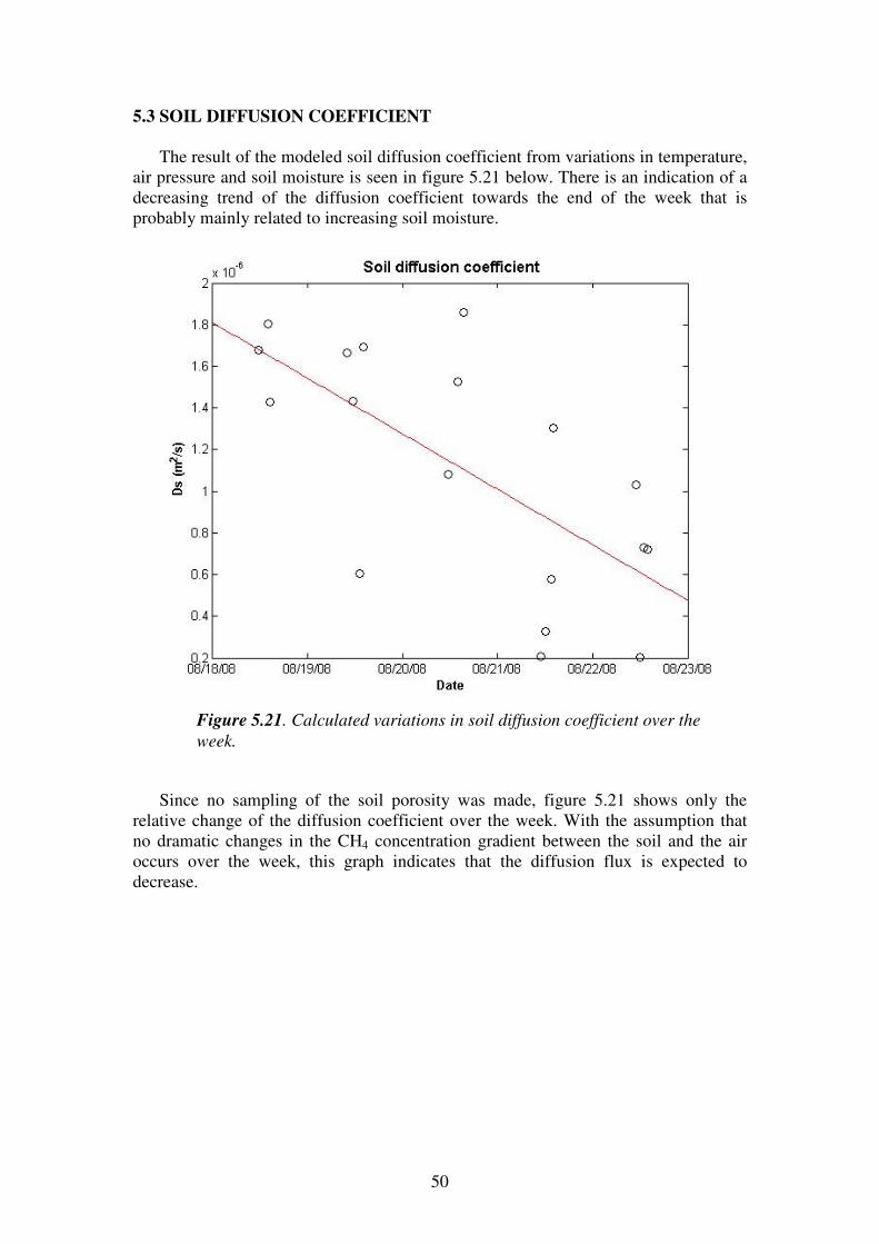
5.3 SOIL DIFFUSION COEFFICIENT

The result of the modeled soil diffusion coefficient from variations in temperature,

air pressure and soil moisture is seen in figure 5.21 below. There is an indication of a decreasing trend of the diffusion coefficient towards the end of the week that is probably mainly related to increasing soil moisture.

Since no sampling of the soil porosity was made, figure 5.21 shows only the

relative change of the diffusion coefficient over the week. With the assumption that no dramatic changes in the CH4 concentration gradient between the soil and the air occurs over the week, this graph indicates that the diffusion flux is expected to decrease.

Figure 5.21. Calculated variations in soil diffusion coefficient over the

week.

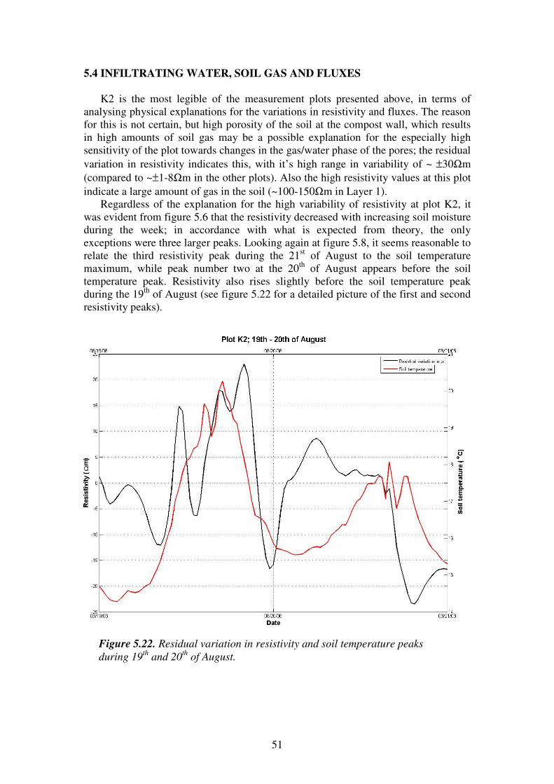
51

5.4 INFILTRATING WATER, SOIL GAS AND FLUXES

K2 is the most legible of the measurement plots presented above, in terms of

analysing physical explanations for the variations in resistivity and fluxes. The reason for this is not certain, but high porosity of the soil at the compost wall, which results in high amounts of soil gas may be a possible explanation for the especially high sensitivity of the plot towards changes in the gas/water phase of the pores; the residual variation in resistivity indicates this, with it’s high range in variability of ~ ±30Ωm (compared to ~±1-8Ωm in the other plots). Also the high resistivity values at this plot indicate a large amount of gas in the soil (~100-150Ωm in Layer 1).

Regardless of the explanation for the high variability of resistivity at plot K2, it was evident from figure 5.6 that the resistivity decreased with increasing soil moisture during the week; in accordance with what is expected from theory, the only exceptions were three larger peaks. Looking again at figure 5.8, it seems reasonable to relate the third resistivity peak during the 21st of August to the soil temperature maximum, while peak number two at the 20th of August appears before the soil temperature peak. Resistivity also rises slightly before the soil temperature peak during the 19th of August (see figure 5.22 for a detailed picture of the first and second resistivity peaks).

Figure 5.22. Residual variation in resistivity and soil temperature peaks

during 19th

and 20th

of August.

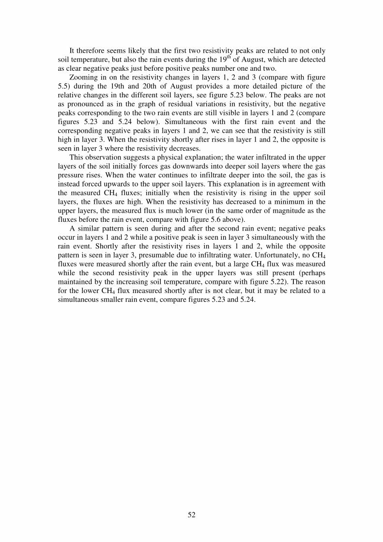
52

It therefore seems likely that the first two resistivity peaks are related to not only soil temperature, but also the rain events during the 19th of August, which are detected as clear negative peaks just before positive peaks number one and two.

Zooming in on the resistivity changes in layers 1, 2 and 3 (compare with figure 5.5) during the 19th and 20th of August provides a more detailed picture of the relative changes in the different soil layers, see figure 5.23 below. The peaks are not as pronounced as in the graph of residual variations in resistivity, but the negative peaks corresponding to the two rain events are still visible in layers 1 and 2 (compare figures 5.23 and 5.24 below). Simultaneous with the first rain event and the corresponding negative peaks in layers 1 and 2, we can see that the resistivity is still high in layer 3. When the resistivity shortly after rises in layer 1 and 2, the opposite is seen in layer 3 where the resistivity decreases.

This observation suggests a physical explanation; the water infiltrated in the upper layers of the soil initially forces gas downwards into deeper soil layers where the gas pressure rises. When the water continues to infiltrate deeper into the soil, the gas is instead forced upwards to the upper soil layers. This explanation is in agreement with the measured CH4 fluxes; initially when the resistivity is rising in the upper soil layers, the fluxes are high. When the resistivity has decreased to a minimum in the upper layers, the measured flux is much lower (in the same order of magnitude as the fluxes before the rain event, compare with figure 5.6 above).

A similar pattern is seen during and after the second rain event; negative peaks occur in layers 1 and 2 while a positive peak is seen in layer 3 simultaneously with the rain event. Shortly after the resistivity rises in layers 1 and 2, while the opposite pattern is seen in layer 3, presumable due to infiltrating water. Unfortunately, no CH4 fluxes were measured shortly after the rain event, but a large CH4 flux was measured while the second resistivity peak in the upper layers was still present (perhaps maintained by the increasing soil temperature, compare with figure 5.22). The reason for the lower CH4 flux measured shortly after is not clear, but it may be related to a simultaneous smaller rain event, compare figures 5.23 and 5.24.

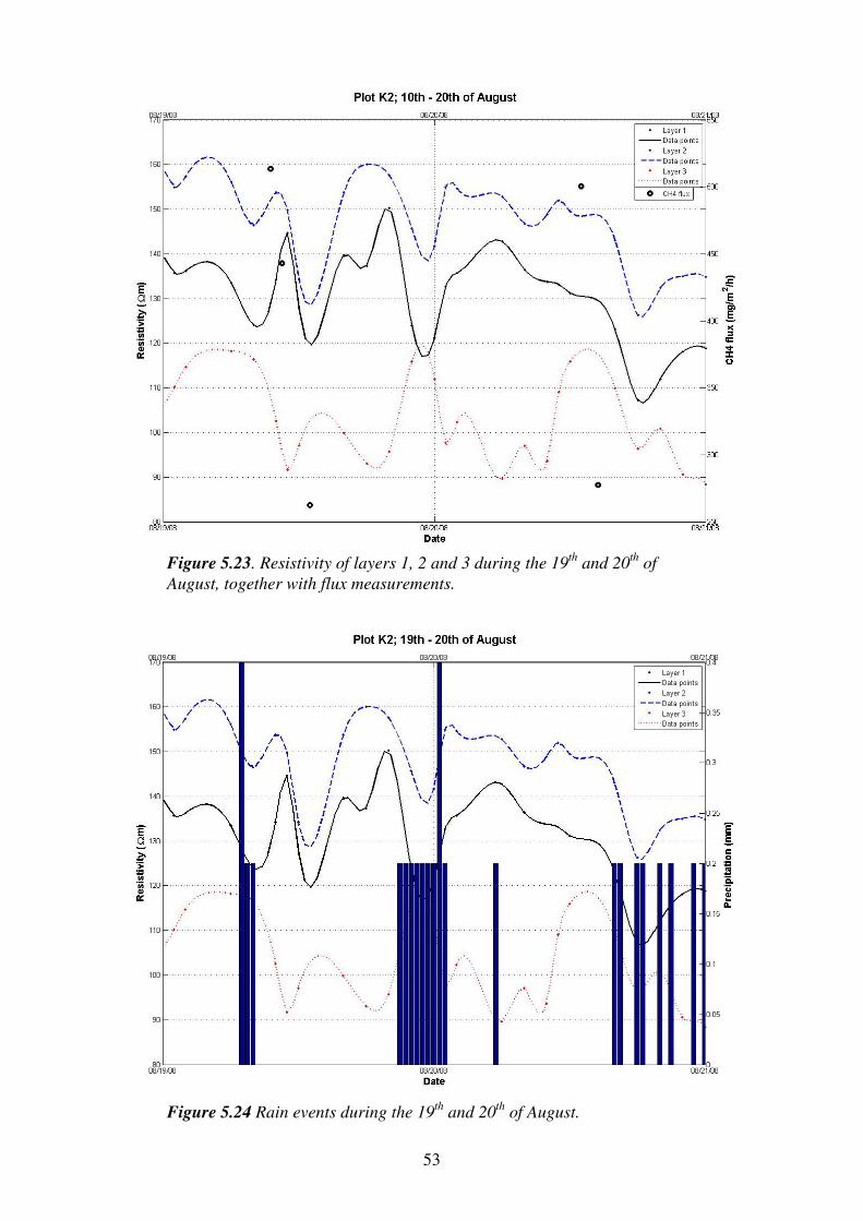
53

Figure 5.23. Resistivity of layers 1, 2 and 3 during the 19th

and 20th

of

August, together with flux measurements.

Figure 5.24 Rain events during the 19th

and 20th

of August.

54

6. DISCUSSION

6.1 THE TEMPERATURE INFLUENCE ON SOIL GAS AND FLUXES

In all measurement plots presented above, soil temperature has proved more or

less to determine the pattern of the resistivity changes of the upper soil layers. This is especially evident at plots K1, K4 and K5.

It is clear that the soil temperature affects the resistivity measured in two different ways; a technical way in which resistivity is proportional to the inverse of the temperature (expression (2.7), a known fact that is caused by the faster mobility of ions with increasing temperatures. The additional effect of the variations in temperature seen in the residual resistivity graphs above is very likely related to physical changes of the gas in the soil pores.

If the ideal gas law (expression 2.9) can be applied to describe the gas present in the soil pores, it can be proposed that the gas pressure in the soil follows the same diurnal pattern as the soil temperature (assumed that the study volume is kept constant, which is the case in all graphs above, and that the transport of gas between the volume and the surroundings is neglible compared to the amount of gas in the study volume).

Increasing gas pressure in the soil pores is likely to cause an increase in resistivity of the soil, since gas itself is a poor carrier of electricity and an increasing pore pressure complicates the transport of charge with e.g. water across the pores.

Increasing gas pressure in the soil causes a larger pressure gradient between the soil and the atmosphere and favors fluxes by pressure flow. 6.2 NEGATIVE CH4 FLUXES

The explanation for the negative CH4 fluxes here is probably related to oxidation

of CH4 in the upper soil layers. Different amounts of gas are emitted at irregular locations around the landfill, but once emitted the wind carries the gas along the soil surface in the direction of the winds. When the static chambers are placed upon the soil, there is an ambient concentration of CH4 in the air. However, if no CH4 is emitted from the soil during the sampling and a simultaneous linear increase of CO2 occurs, it is logical that we get a linear decreasing concentration of CH4 in the air samples, i.e. a negative CH4 flux.

It was initially assumed that the landfill gas at this site consisted of nearly equal amounts of CH4 and CO2 (see chapter 2.2.1 above). However, it is still realistic that CH4 is oxidized in the upper soil layers at certain areas around the landfill, especially during dry soil conditions and at measurement plots where the fluxes are generally small and oxidation has enough impact to change fluxes from being positive to negative.

Since the CO2 concentrations in the air samples were not analysed in the lab, the interpretation of the gas emissions must be based on the size of the CH4 fluxes. It is assumed that CH4 oxidation is neglible at the measurement plots where CH4 fluxes are generally very high (plots K2 and K3). At the remaining measurement plots, both large positive and large negative fluxes are assumed to indicate a high gas flow.

55

6.3 BEHAVIOUR OF GAS FLUXES AT LANDFILLS

Diffusion in the air filled soil pores has been stated as the main transport

mechanism in natural ecosystems under normal soil conditions, when no major changes in barometric pressure occur (Jassal et al 2005). The surface flux has often been modelled as a function of soil moisture and temperature, which relates to microbial activity (Tang et al. 2003).

In landfills, the soil moisture content of the upper soil is one of the most important factors controlling gas emissions, since high soil moisture content in soil pores can more or less constrain gas from diffusing to the atmosphere. Studies have shown that the soil moisture also affects the CH4 oxidation capacity of the upper soil layers. The relationship found between increasing soil moisture and increasing CH4 emissions is explained by the decrease of oxygen in the soil pores with increasing soil moisture (Boeckx et al 1996).

Another study, in which the Filborna landfill was one of the investigated sites, has shown that the CH4 oxidation in landfills increases also with increasing soil temperature, due to microbial activity (Börjesson et al. 2004). Besides the most important environmental factors soil moisture and soil temperature, CH4 oxidation is also controlled by soil texture, CH4 and oxygen concentrations and nutrients (Scheutz et al. 2004).

From earlier studies, we would therefore expect a relationship between soil temperature, soil moisture and CH4 emissions. At the measurement plots where negative fluxes (i.e. CH4 oxidation) occur, it is expected that the fluxes becomes less negative or positive with increasing soil temperature and soil moisture, to a certain limit. If the soil moisture becomes high enough, it will instead act as a barrier for gas transport of both CH4 and CO2 to the atmosphere, and the CH4 fluxes are expected to decrease (Boeckx et al 1996).

As discussed above, there are indications in the data from plot K2 that the largest CH4 fluxes occur due to advection rather than diffusion processes. With these results in mind, the pattern of the fluxes measured at plots K1 and K3 can be proposed as concordant to what was seen in plot K2; the maximum fluxes occur at midday during the 19th and/or 20th of August, after the two rain events that caused the maximum fluxes in plot K2. In plot K1, this is the only positive flux measured. Although the flux data is very limited here, it can indicate that the positive flux occur due to advection after rainfall, in an area of the landfill where oxidation normally consumes the CH4 before it is emitted to the atmosphere.

Also the resistivity peaks at the 20th of August in plots K4 and K6 occur immediately after the rainfall, but before the temperature maximum. This means that the pattern of the soil gas behavior according to the resistivity data is concordant in all measurement plots except plot K5 (although the flux data is not sufficient at plots K4 and K6 to relate the resistivity peaks to increased CH4 emissions).

The reason that plot K5 differs in it’s behavior from the rest of the plots is not clear, but it can be suggested that the cover material on the plot has an impact. On the surface, plot K5 consisted of a lot of clay. High presence of clay could explain why so few flux measurements were successful here compared to the other plots. Water also infiltrates slower through clay than through more porous materials; this could be an explanation to the fact that the measured resistivity at plot K5 shows no response to rain events and seems only controlled by the soil temperature.

56

There is a possible reason to the generally higher values of resistivity and CH4 fluxes at plots K2 and K3 are likely. There is a gas pipe and a gas well running in between these plots, around which a compost wall with high porosity runs according to the description of the waste composition. Both high gas accumulations due to high porosity favors gas transport and leads to high measured resistivity values.

If the maximum fluxes corresponding to presumed advection transport after rain events is excluded, general trends in the fluxes over the weeks can be vaguely indicated. At plots K2 and K3 there are decreasing trends of the size of the fluxes, which is in agreement with the decreasing trend of the diffusion coefficient. At plot K4, a tendency of increasing fluxes, going from negative towards positive, can be seen. It can be proposed that this is a result of the increasing soil moisture during the week, which brings less oxide in the soil pores. As a consequence of decreasing CH4 oxidation, the measured CH4 flux becomes larger during the week. In plots K1, K5 and K6, the number of measured fluxes is so low that it is difficult to see any trends. In addition, the variability in size of the fluxes are so small in these plots, that possible measurement errors described in chapter 3.2.3 can have a significant influence on the results.

The on average higher fluxes measured in July compared to August could possibly be explained by the higher average soil temperature during the measurement period in July (18.7°C) compared to in August (16.0°C). The total sum of precipitation during the week in July was 30.4mm, compared to 12.2mm in August, which in theory also favor a larger gas transport in July.

6.4 UNCERTAINTIES IN THE ANALYSIS OF THE RESISTIVITY DATA

As already indicated in chapters 2.1.1 and 2.1.2 above, there are many reasons for

handling resistivity data with care, especially at the detailed scale necessary for this application. The pol-dipol electrode configuration and the robust inversion method used for all soil models in this experiment should provide as good conditions as possible for obtaining reliable results.

A technical problem with the data is that during the inversion process, different soil models can give rise to the same pseudosection. But since the same method and parameters are used in all inversions from the investigation, it can be assumed that the changes in resistivity over time correspond to real changes in the ground.

The decision of interpolating the resistivity data to smooth out the in some cases steep borders between the coordinate values in the model should not cause any biases, since a linear interpolation does not create any data that does not exist. Instead it improved, in my opinion, the data analysis, since it enhanced the probability to fetch the variations in the ground right below the static chamber measurement plots.

As a result of the linear interpolation, it was also possible to identify the “borders” of the “gas pockets” below measurement plots K1, K2 and K3 through selecting a minimum value of the data cells in the matrix to be included in the analysis. It is of course a source of uncertainty to, in some meaning randomly, limit the data in this way. However, it was done with the assumption that higher resistivity values correspond to higher gas content in the soil pores. Even though physical changes exist and have an influence also in the surrounding soil, it was assumed that this was neglible in relation to the presumed main changes that would occur in the center of the “gas pockets”.

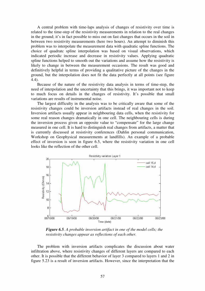
57

A central problem with time-laps analysis of changes of resistivity over time is related to the time-step of the resistivity measurements in relation to the real changes in the ground; it’s in fact possible to miss out on fast changes that occurs in the soil in between two resistivity measurements (here two hours). An attempt to diminish this problem was to interpolate the measurement data with quadratic spline functions. The choice of quadratc spline interpolation was based on visual observations, which indicated periodic increase and decrease in resistivity values. Applying quadratic spline functions helped to smooth out the variations and assume how the resistivity is likely to change in between the measurement occasions. The result was good and definitively helpful in terms of providing a qualitative picture of the changes in the ground, but the interpolation does not fit the data perfectly at all points (see figure 4.4).

Because of the nature of the resistivity data analysis in terms of time-step, the need of interpolation and the uncertainty that this brings, it was important not to keep to much focus on details in the changes of resistivity. It’s possible that small variations are results of instrumental noise.

The largest difficulty in the analysis was to be critically aware that some of the resistivity changes could be inversion artifacts instead of real changes in the soil. Inversion artifacts usually appear in neighbouring data cells, when the resistivity for some real reason changes dramatically in one cell. The neighbouring cells is during the inversion process given an opposite value to “compensate” for the large change measured in one cell. It is hard to distinguish real changes from artifacts, a matter that is currently discussed at resistivity conferences (Dahlin personal communication, Workshop on Geophysical measurements at landfills). An example of a probable effect of inversion is seen in figure 6.5, where the resistivity variation in one cell looks like the reflection of the other cell.

The problem with inversion artifacts complicates the discussion about water infiltration above, where resistivity changes of different layers are compared to each other. It is possible that the different behavior of layer 3 compared to layers 1 and 2 in figure 5.23 is a result of inversion artifacts. However, since the interpretation that the

Figure 6.5. A probable inversion artifact in one of the model cells; the

resistivity changes appear as reflections of each other.

58

resistivity variation here is caused by water infiltration is in good agreement with both precipitation and flux data, the discussion should not be dismissed. In my opinion, there are matters, besides the argument that it is physically likely that the variations could be real, that speak against inversion artifacts. For example, there are no contradictions between the resistivity variations in layers 1 and 2; inversion artifacts could as well appear here, as between layers 2 and 3. Additionally, there are several examples in the same graph where really large variations in layer 3 are not reflected in layer 2 (e.g. large positive resistivity peak in layer 3 on early 21st of August, see figure 5.5 above). 6.5 UNCERTAINTY OF THE RESULTS

The general problems with the static chamber method, regarding the impact of the closed chambers on the environment, is probably largest during rainfall since the chambers then block the precipitation to reach the soil. Rain events, according to the current results, seem to play an important role for varying CH4 fluxes.

It is difficult to evaluate how large uncertainty the mechanical disturbances during the measurement bring. Possibly could some of the measured fluxes, which were excluded because the increasing concentration was not linear, have been failed as a consequence of mechanically forced gas from the soil during the placement of the chambers on the soil surface. However, the CH4 fluxes presented in the results above were all linear with satisfying R2-values, which means that this kind of mechanical disturbance probably plays a minor role in the results.

As stated in chapter 3.2.3, it is possible that the clay sealing of the chambers to the ground creates errors in the flux data. Whereas the measured fluxes are larger or smaller than the natural fluxes for this reason is probably impossible to estimate. The best solution of this problem is of course to use better equipment.

There is also an uncertainty related to the analysis of the gas samples in the gas chromatograph, as well as approximations used when calculating the gas fluxes.

Due to all these sources of uncertainty in the size of the fluxes, it should be avoided to analyse the fluxes in detail. However, the errors should not be too large for a relative analysis as the one presented here. The errors in the flux data are probably not larger than errors in the soil moisture and precipitation data. It is important to stress that the uncertainty in the data affects most of the results presented in chapter 5 quantitatively. These should thus be treated as general trends and indications of processes, rather than verified relationships. The only statistically significant result is that the fluxes at measurement plots K2 and K3 differs from the fluxes measured at all other plots.

59

6.6 FUTURE IMPROVEMENTS OF THE METHODOLOGY

The idea of using electrical resistivity measurements together with flux

measurements appears to be useful to understand the behavior of gas in heterogeneous soils. However, a number of adjustments of the methodology could probably improve the results and perhaps lead to more general and perhaps statistical relationships.

The number of unvisibal fluxes measured with static chambers during this project turned out to be relatively low, despite the fact that around 140 measurements were done during two weeks. Simultaneously with the static chamber measurement in July, the resistivity data was unfortunately missing, and several of the flux measurements had to be excluded because the change in concentration was not linear. If a similar project would be performed in the future, it would be benefited by a higher number of flux measurements. Better equipment (e.g. frames on the measurement plots for the static chambers) would probably yield more significant fluxes and fewer disturbances on the soil. Additionally, it’s preferable that both CO2 and CH4 is analysed in the gas chromatograph, since CH4 oxidation seems to have played an important role at some of the measurement plots here.

Soil moisture is probably one of the most important controllers of soil gas movements and emissions at landfills. Continuous measurements of soil moisture would therefore improve the analysis noticeable. Sampling of soil porosity (and possibly soil gas concentration) at different locations and soil depths around the landfill would also provide a more detailed analysis.

With appropriate handling and interpolation of the resistivity data, it has been shown that it can provide sufficient information for an analysis of this kind, even though the information must be used with care. The large time-step of two hours between the measurements was not a problem in this study. Possibly, a smaller investigation area with less resistivity lines and electrodes in the experimental arrangement could be used, if any future study aims to focus on gas transport and emissions in particular. This approach would reduce the time required for each measurement and provide a data set with smaller time-steps, which in turn could lead to a perhaps more detailed analysis.

60

7. CONCLUSIONS

It is possible to obtain knowledge about soil gas behavior and emissions at landfills through a combination of the geophysical method electrical resistivity, surface flux measurements and environmental logging.

The results have shown that resistivity data can visualize how the soil gas is affected by soil temperature, rain events and general changes in soil moisture. This visualization has contributed to an interpretation of advection versus diffusion transport of gas from the soil to the atmosphere, which is possibly one of the explanations to the temporally varying gas fluxes at landfills.

At this particular site, the main pattern of gas dynamics in the ground relates to diurnal variations in soil temperature, which affects the gas pressure in the soil pores and seems to increase and decrease the extension of the gas assimilations. Water infiltration creates pressure imbalances in soil layers, which probably force the gas upwards to the atmosphere.

There are indications in the results that the diffusion transport of gas decreases in agreement with the modeled diffusion coefficient. The CH4 oxidation in the upper soil layers shows a tendency to decrease with increasing soil moisture. The results also suggest that advection transport of gas occurs after intense rain events. A longer time-series and more flux measurement replicates are necessary to find statistically significant results.

The study suggests that the in general largest CH4 fluxes occur in the vicinity of gas assimilations in the ground, which are indicated by particularly high resistivity values.

61

8. REFERENCES Litterature and articles Barber, C., Davis, G.B., Briegel, D., Ward, J.K. 1990: Factors controlling the

concentration of CH4 and other volatiles in groundwater and soil-gas. In: Journal of Contaminant Hydrology, 5 (1990), 155-169. Billings, S.A., Richter, D.D., Yarie, J. 2000: Sensitivity of soil CH4 fluxes to reduced

precipitation in boreal forest soils. In: Soil Biology & Biochemistry 32 (2000), 1431-1441. Boeckx, P., Van Cleemput, O., Villaralvo, I. 1996: CH4 emission from a landfill and

the CH4 oxidizing capacity of its covering soil. In: Soil Boil. Biochem. Vol. 28, No. 10/11. 1397-1405. Bouye, J-M., Budka, A., Courant, P., Ripaud, F. & Moreau, S. 2007: Towards the

determination of volumetric water content in waste body from electrical resistivity:

laboratory tests. In: Proceedings Sardinia 2007, Eleventh International Waste Management and Landfill Symposium. S. Margherita di Pula, Cagliari, Italy; 1-5 October 2007. Börjesson, G., Sundh, I., Svensson, B. 2004: Microbial oxidation of CH4 at different

temperatures in landfill cover soils. In: FEMS Microbiology Ecology 48 (2004), 305-312. Campbell, G.S. 1998: An introduction to environmental biophysics. New York, USA. Chapin III, F.S, P.A. Matson and H.A. Mooney, 2002: Principles of Terrestrial

Ecosystem Ecology. New York, USA. Crawford, J.F. & P.G. Smith, 1985: Landfill technology. London, UK. Choi, J-W., Tillman, F.D., Smith, J.A. 2002: Relative Importance of Das-Phase

Diffusive and Advective Trichloroethene (TCE) Fluxes in the Unsaturated Zone under

Natural Conditions. In: Environmental Science & Technology, 2002, 36 (14), 3157-3164. Christensen, T.H. (red.), 1998: Affaldsteknologi. Copenhagen, Denmark. Dahlin, T. 1993: On the Automation of 2D Resistivity Surveting for Engineering and

Environmental Applications. Department of engineering geology, Lund Institute of Technology, Lund University. Thesis 1993. Lund. Dobrin, M.B. 1976: Introduction to geophysical prospecting. USA.

62

Europeiska Unionens råd, 1999: Rådets direktiv 1999/31/EG av den 26 april 1999 om

deponering av avfall. In: Europeiska gemenskapernas officiella tidning. Publikationsbyrån, Luxembourg. Fang, C., Moncrieff, J.B. 1999: A model for soil CO2 production and transport 1:

Model development. In: Agricultural and forest metrology 95 (1999) 225-236. Foster, P., V Ramaswamy, P. Artaxo, T. Berntsen, R. Betts, D.W. Fahey, J. Haywood, J. Lean, D.C. Lowe, G. Myhre, J. Nganga, R. Prinn, G. Raga, M. Schulz and R. Van Dorland, 2007: Changes in Atmospheric Constituents and in Radiative Forcing. In:

Climate Change 2007: The Physical Science Basis. Contribution of Working Group I

to the Fourth Assessment Report of the Intergovernmental Panel on Climate Change [Solomon, S., D. Qin, M. Manning, Z. Chen, K.B. Averyt, M. Tignor and H.L. Miller (eds.)]. Cambridge University Press, Cambridge, United Kingdom and New York, NY, USA. Georgaki, I., Soupios, P., Sakkas, N., Ververidis, F., Trantas, E., Vallianatos, F. & Manios, T. 2007: Evaluating the use of electrical resistivity imaging technique for

improving CH4 and CO2 emission rate estimations in landfills. In.: Science of the total environment 389 (2008), 522-531. Harbison, G.M. 2008: The true “green” benefit of alternative fuels. In: Ceramic Industry; Jan 2008; 158,1; ABI/INFORM Global pg. 119. Hashemi, M., Kavak, H.I., Tsotsis, T.T., Sahimi, M. 2002: Computer simulation of

gas generation and transport in landfills – I: quasi-steady-state condition. In: Chemical Engineering Science 57 (2002) 2475 – 2501. Jassal, R., Black, A., Novak, M., Morgenstern, K., Nesic, Z., Gaumont.Guay, D. 2005: Relationship between soil CO2 concentrations and forest-floor CO2 effluxes.

In: Agricultural and Forest Meteorology 130 (2005) 176–192. Jolly, J., Barker, R.D., Beaven, R.P., Herbert, A.W. 2007: Time lapse electrical

imaging to study fluid movement within a landfill. In: Proceedings Sardinia 2007, Eleventh International Waste Management and Landfill Symposium, S. Margherita di Pula, Cagliari, Italy; 1 - 5 October 2007. Keller, G.V., Frischknecht, F.C. 1966: Electrical methods in geophysical prospecting. London Keary, P. & Brooks, M. 1991: An Introduction to Geophysical Exploration. Second

edition. London, UK. Kjeldsen, P. & Fischer, E. 1995: Landfill gas migration – field investigations at

Skellingsted Landfill. Waste management & Research, vol. 13, 467-484. LaBreque, D.J., Ramirez, A.L., Daily, W.D., Binley, A.M., Schima, S.A. 1996: ERT

monitoring of environmental remediation processes. In: Measurement Science and Technology 7 (1996) 375-383)

63

Lamborn, J. 2007: Developing a landfill gas model. In: Proceedings Sardinia 2005, Tenth International Waste Management and Landfill Symposium. S. Margherita di Pula, Cagliari, Italy; 3-7 October 2005. Liang, B., Liu, L., Xue, Q., Zhao, Y. 2008: Porosity Prediction with Settlement and

Biodegradation in Municipal Landfill. In: Bioinformatics and Biomedical Engineering, 2008. ICBBE 2008. The 2nd International conference on. Loke, M.H., Acworth, I., Dahlin, T. 2003: A comparison of smooth and blocky

inversion methods in 2D electrical imaging surveys. In: Exploration geophysics (2003) 34. Maurice, C. 1998: Landfill Gas Emission and Landfill Vegetation. Licentiate thesis. Luleå University of Technology. Department of Environmental Engineering. Division of Landfill Science and Technology. Luleå Marcoux, M.A., Adib, R., Lagier, T. & Gourc, J-P. 2007: Monitoring of leachate

recirculation in a bioreactor landfill: comparison of lysimeter and resistivity

measurements. In: Proceedings Sardinia 2007, Eleventh International Waste Management and Landfill Symposium. S. Margherita di Pula, Cagliari, Italy; 1-5 October 2007. Miljödepartementet, 2001: Förordning (2001:512) om deponering av avfall. :§10,§13

Stockholm. Moon, S., Nam, K., Kim, J.Y., Hwan, S.K., Chung M. 2008: Effectiveness of compacted soil liner as a gas barrier layer in the landfill final cover system. In: Waste Management 28 (2008) 1909-1914. Moreau, S., Bouye, J-M., Duquennoi, C., Barina, G. & Oberti, O. 2004: Electrical

resistivity survey to investigate biogas migration under leachate recirculation events.

Waste 2004; Integrated waste management and pollution control policy and practice, research and solutions, Stratford-upon-Avon, September, 2004. O’Leary, P. & Walsh, P. 2002: Landfill gas movement, control and energy recovery. Waste age; Mar 2002; 33,3: ABI/INFORM Global. Parasnis, D.S. 1986: Principles of Applied Geophysics. London, UK. Rosqvist, H., Dahlin, T., Linders, F. & Meijer, J-E. 2007: Detection of water and gas

migration in a bioreactor landfill using geoelectrical imaging and a tracer test. In: Proceedings Sardinia 2007, Eleventh International Waste Management and Landfill Symposium. S. Margherita di Pula, Cagliari, Italy; 1-5 October 2007. Samuelsson, J., Galle, B. & Börjesson, G. 2005: Slutrapport STEM projekt nr

P10856-4. ”Metan från avfallsuppslag i Sverige”. Chalmers Tekniska Högskola, Göteborg och Linköpings Universitet, Linköping.

64

Sanchez, R., Hashemi, M., Tsotsis, T.T., Sahimi, M. 2006: Computer simulation of gas generation and transport in landfills II: Dynamic conditions. In: Chemical Engineering Science 61 (2006) 4750-4761. Sharma, P.V. 1997: Environmental and engineering geophysics. Cambridge, UK. Scheutz, C., Kjeldsen, P. Environmental Factors Influencing Attenuation of CH4 and

Hydrochlorofluorocarbons in Landfill Cover Soils. In: J. Environ. Qual. 33, 72-79. Stepniewski, W., Horn, R., Martyniuk, S. 2002: Managing soil biophysical properties

for environmental protection. In: Agriculture, Ecosystems and Environment 88 (2002) 175-181. Tang, J., Baldocci, D.D., Qi, Y., Xu, L. 2003: Assessing soil CO2 efflux using

continuous measurements of CO2 profiles in soils with small solid-state sensors. In: Agricultural and Forest Meteorology 118 (2003) 207–220. Visscher, A.D., Cleemput, O.V. 2003: Simulation model for gas diffusion and CH4

oxidation in landfill cover soils. In: Waste Management 23 (2003). 581-591. Internet references Naturvårdsverket

1. 2008.02.12: Principer för avfallshantering (http://www.naturvardsverket.se/sv/Produkter-och-avfall/Avfall/Mal-strategier-och-resultat/Principer-for-avfallshantering/)

2. 2008:03.26: Ramdirektivet för avfall (http://www.naturvardsverket.se/sv/Produkter-och-avfall/Avfall/Lagar-och-regler-om-avfall/Ramdirektivet-for-avfall/)

Project collaborators Dahlin, Torleif, Engineering Geology at Lund University Leroux, Virginie, NSR Återvinning Lindsjö, Magnus, NSR Återvinning Månsson, Carl-Henrik, Tyréns AB Rosqvist, Håkan, NSR Återvinning Svensson, Mats, Tyréns AB Project report

Dahlin, T., Johansson, S., Leroux, V., Lindsjö, M., Månsson, C-H., Rosqvist, H., Svensson, M. 2009: Detektering av gas i deponier med resistivitet. Published at: 1. Avfall Sverige (http://www.avfallsverige.se/m4n) 2. SGC ( http://www.sgc.se/ )

65

Workshop on Geophysical measurements at landfills Malmö, 18-19 November, 2008. Arranged within the project by NSR Återvinning, Tyréns AB and Lund University. Participants: University of Southhampton, Cemagref, International waste working group, SGF.

electrical resistivity as a tool for analyzing soil gas...

Documents