eiscat observations of ion composition and temperature anisotropy in the high-latitude f-region

EISCAT observations of ion composition and temperature anisotropy in the high-latitude F-region

M. LOCKWOOD,* 1. W. MCCREA,* G. H. MILLWARD,? R. J. MOFFETT~ and H. RISHBETH~

*Rutherford Appleton Laboratory, Chilton, Didcot, OX1 1 OQX, U.K. : t Department of Applied and Computational Mathematics, University of Sheffield, Sheffield, SIO 2TN, U.K.; $ Department of

Physics, University of Southampton, Southampton, SO9 SNH, U.K.

(Received i?z $nal ,fornz 18 June 1992 ; ncceped 29 Jufy 1992)

Abstract-The papers by WINSER et al. [(1990) J. afnm. terr. P&Y. 52, 5011 and H~~GGSTR~M and COLLIS [(1990) J. atmos. terr. Whys. 52,519] used plasma flows and ion temperatures, as measured by the EISCAT tcistatic incoherent scatter radar, to investigate changes in the ion composition of the ionospheric F-layer at high latitudes, in response to increases in the speed of plasma convection. These studies reported that the ion composition rapidly changed from mainly O+ to almost completely (> 90%) molecular ions, following rapid increases in ion drift speed by > 1 km s- ‘. These changes appeared inconsisent with theoretical considerations of the ion chemistry, which could not account for the large fractions of molecular ions inferred from the obsevations. In this paper, we discuss two causes of this discrepancy. First, we ce- evaluate the theoretical calculations for chemical equilibrium and show that, if we correct the derived temperatures for the effect of the molecular ions, and if we employ more realistic dependenees of the reaction rates on the ion temperature, the composition changes derived for the faster convection speeds can be explained. For the Winsec et al. observations with the radar beam at an aspect angle of # = 54.7’ to the geomagnetic field, we now compute a change to 89% molecular ions in ~2 min, in response to the 3 km s- ’ drift. This is broadly consistent with the observations. But for the two cases considered by H~ggstc~m and Collis, looking along the field line (4 = O”), we compute the pco~ction of molecular ions to be only 4 and 16% for the observed plasma drifts of 1.2 and 1.6 km s- ‘, respectively. These computed proportions ace much smaller than those derived experimentally (70 and 90%). We attribute the differences to the effects of non-Maxwellian, anisotropic ion velocity distribution functions. We also discuss the effect of ion composition changes on the various radar observations that report anisotcopies of ion temperature.

1. INTRODUCTION

Two recent papers in this journal [WINSER et al., 1990, and HKGGSTR~M and COLLIS, 1990 (henceforth WEA

and H&C)] used EISCAT UHF radar data to study the changes in ion composition that accompany increases of plasma drift velocity and ion temperature in the ionospheric F-layer. These events ace known as ‘ion heating events’, and typically last for tens of minutes. They are caused by enhanced electric fields which, on the dayside, appear to be triggered by changes in the interplanetary magnetic field, as in the example discussed by RISHBETH et al. (1985).

In their analysis of such events, both WEA and H&C estimate the ion temperature in the lower F-

layer from the simplified ion energy balance equation

I, = T,+(m,/3k)jV,-V,j2 (1)

(in which we neglect electron-ion collisions and other small terms). Here T, is the average, three-dimensional ion temperature, T, is the temperature of the neutral thermospheric gas, m, is the mean mass of the neutral

gas, k is Boltzmann’s constant, V, is the bulk velocity of the ion gas and V, is the velocity of the neutral gas (ST-MAURICE and HANSON, 1982). Of these quantities, T, and Vi are measured by the radar, while T, and V, can in principle be measured by an optical inter- ferometer (e.g. WINSER et al., 1988), though in the cases analysed by WEA and H&C, no such optical data were available. We assume that initially V, = V, and hence T, = T,, and also (because of the bulk of the neutral air) that V, and T, remain constant during the event. These assumptions (especially that V,, = V, before the event) may be questioned since, even under quiet conditions at high latitudes, V, and V, may differ by 100 m s -’ or so; furthermore, T, may exceed T,

because of the influence of the electron gas. Never- theless, it is almost certainly true that, provided conditions have been reasonably quiet for some time pre-

viously, [Vi -V,I’ is much greater during the event than beforehand, so (I) can be used to compute the increase of 7;. The value of m, is taken from an atmo- spheric model, such as MSIS-86 (HEDIN, 19871, and

the model also provides a check on the value of T,, The incoherent scatter technique allows the deter-

895

896 M. LOCKWOOD et al.

mination of ion temperature, but it is important to understand precisely what is measured. The technique can only give info~ation about the distribution of ion velocities along the radar beam, which is charac- terised by a line-of-sight temperature T+. It is fre- quently assumed that the three-dimensional ion velocity distribution is isotropic, in which case T+ is the same as the average, three-dimensional temperature used in the energy balance equation (1). However, as discussed in Section 3.1, there is now considerable evidence, both theoretical and experimental, that the ion velocity distribution is not isotropic when the ion heating is strong. As a result, the measured value of T, in general depends on the aspect angle (p between the radar beam and the geomagnetic field. We can define an ‘anisotropy factor’

u = TJT,. (2)

In addition, the analysis of the received incoherent scatter spectrum requires two assumptions to be made. First, a form of the dist~bution of the line-of- sight velocities must be adopted. It is often assumed that this distribution is Maxwellian, which yields an estimate Tern for the line-of-sight ion temperature. However, the theory and calculations discussed in Section 3 show that this assumption, too, becomes invalid when the ion heating is strong, particularfy at large values of 4. Hence it is useful to define a ‘non- Maxwellian’ factor

b = T+IT+,,,. (3)

The second necessary assumption is that of the ion mass. The theory of incoherent scatter shows that the width of the spectrum is approximately proportional to ,/(T+/mJ. Hence we can write

T&mi E 7$&ria (4)

where the dash denotes a temperature derived using an assumed value mi, for the ion mass, and mi is the real ion mass. From (2), (3) and (4) we can write

TJmi x (b/a) T&,,jmiat (5)

Theory shows that in general b < 1, and decreases with increasing 4 and Vi. If the ion velocity distribution is anisotropic, as shown by the EISCAT data (Sec- tion 3.3), the ‘anisotropy parameter’ a > 1 if cp > 54.7”, but n < 1 if # < 54.7’ (where 54.7” = arc sin,,/($). In practice (5) is a good approximation, though it is not exact because the spectral width depends on other factors, in particular the electron temperature T, (SUVANTO et al., 1989). From (I) and (5) we can derive the real ion mass

m, = m,,lT,+(t?l,/3k)lVi-V,12)l((b/a)T6~j. (6)

This equation is, in essence, the origin of the method used by WEA and I-I&C. However, both WEA and H&C avoid making the approximation inherent in equation (4): H&C achieve this by carrying out a second analysis with the ion temperature set by the frictional heating equation (1) and fitting for the ion composition ; WEA repeat the analysis for the com- plete range of ion compositions and then select mi to give the ‘real’ T, that satisfies (1). Equation (6) does contain approximations, and its application to real data may of course be affected by noise in the data, hut it provides a basis for investigating composition effects.

In this paper, we investigate the observations of changes to the composition of the ion gas, as reported by WEA and H&C. In Section 2 we compare the experimentally derived composition with computations for chemical equilibrium. The results of WEA are broadly consistent with the equilibrium computations, the remaining difference (about 10%) being explicable in terms of departures from chemical equilib~um and/or experimental error. However, the molecular ion fractions reported by H&C are found to be an order of magnitude larger than computed for chemical equilibrium. Consequently, we assess the effect of anisotropy of the ion velocity distribution function on these observations in Section 3. Finally, in Section 4 we evaluate the converse effect, namely, that of ion composition changes on the various radar observations that show anisotropy of the ion gas.

2. ION CHEMISTRY

In this section we briefly discuss the assumption that the F-layer ion composition is determined by chemical equilibrium (Section 2.1). We then revise the theoretical calculations of ion composition made by WEA (Section 2.2), using improved values for the rate coefficients and corrected values of ion temperature, and apply a similar analysis to the events studied by H&C (Section 2.3).

2.1. The assumption of chemicaI equilibrium

For our theoretical investigation of the ion composition, we assume the ions to be in chemical equilibrium. This should be a good approximation for the lower F-layer by day, but must be used with caution for the ion heating events discussed in this paper. For the winter night-time event studied by WEA, it has to be questioned whether the O+ ions could be in chemical equilibrium at all, because of the lack of an obvious source of ionisation. However, the assumption of chemical equilibrium seems to be a reasonable

Temperature anisotropy in the high-latitude F-region 897

approximation for the molecular ions (RISHBETH et al., 1972), which is what matters most in the present analysis. For the afternoon events studied by H&C, the temperature and velocity data were recorded at a height of 279 km which, in the July event, was above the height of the F2 peak (estimated to be about 200 km). In this case, the atomic ion distribution would largely be controlled by plasma diffusion: again, the ‘chemical equilibrium’ computation is a better guide to the molecular ion distributions than to the O+ distribution.

The resulting linear loss coefficient for the loss of Of by the transfer reactions (7) and (8) is given by

P = B, +8> = K,40J+K,W,I (11)

where n[Xj denotes the number density of the neutral gas X. lfthe molecular ions are in chemical equilibrium (as is probably the case), it is easy to show that the ratio of the NO+ and 0: concentrations is

Apart from transport effects (see below), the uncertainties in the chemical equilibrium calculations include additional O+ loss mechanisms, the use of the MSIS model (the accuracy of which-particularly as regards composition-is not well established at the latitude of EISCAT) and experimental error. The latter may be appreciable because of the low electron density, and hence poor signal-to-noise ratio, during the heating event; this applies particularly to the remote EISCAT receiving sites, and would affect the accuracy of the tristatic velocity measurements.

For the examples considered in this paper, we will show (in Table 1 and Fig. 1) that ,Gz > b, (since n[N,]/n[O,] z 20 and KJK, > O.l), while the dis- sociative recombination coefficients t(, and cl* are very similar. Hence in a steady state N[NO+] > N[O:]. This conclusion is reinforced if we take account of a further important process, namely the production of NO+ by the charge transfer reaction

Transport effects include plasma diffusion and hori- zontal transport. The former is not likely to influence the ion composition at heights well below the F2 peak. The latter may be important if concentrations (etc.) change appreciably within the distance travelled by the ions during their lifetime. Our revised computations (Section 2.2) give a time constant for the conversion of the oxygen ions to molecular ions (l/b) of 1.8 min. This is much shorter than the 15 min derived previously by WEA, and is much more consistent with the observations (fig. 8 of WEA shows a change from almost zero to 100% molecular ions in 1 min). Although the O+ ions only travel a few kilometres during their lifetime, the lifetime of the molecular ions (under the conditions of low electron density in the WEA event) is of order 10’ s, during which time they may travel some 1000 km. Our lack of knowledge of the ‘previous history’ of the plasma presents a difficulty, but this of course is a very com- mon problem in ionospheric studies generally.

N:+O+NO++N (13)

as in the modelling study of MOFFETT et al. (1992). Again assuming chemical equilibrium (though this requires more discussion for the atomic ions ; see Sec- tion 2.3), and using a mean coefficient a = ~(LY, +r,),

2.2. Revision of the calculations by Winser et al.

As discussed by WEA, the in-situ production and decay of molecular ions in the F-region is dominated by the reactions :

Of +O, --* 0: +O (rate coefficient K,) (7)

Of +N2 -+ NO+ + N (rate coefficient K2) (8)

O:+e-+O+O (ratecoefficienta,) (9)

NO+ fe + NfO irate coefficient a,). 1101

(Ti+TJ (103K)

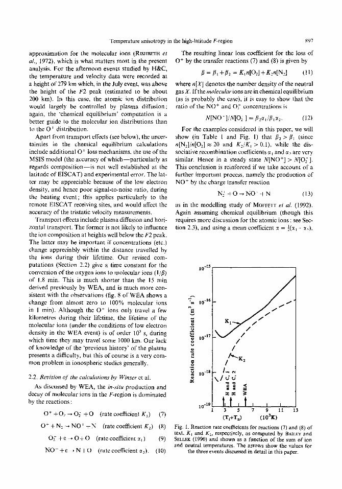
Fig. 1. Reaction rate coefficients for reactions (7) and (8) of text, K, and K,, respectively, as computed by BAILEY and SELLEK (1990) and shown as a function of the sum of ion and neutral temperatures. The arrows show the values for . . .

the three events dlscussed m detail in this paper.


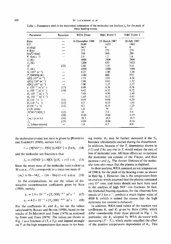
Table 1. Parameters used in the theoretical estimation of the molecular ion fraction f,, for the peak of three heating events

Parameter Equation WEA Event H&C Event 1 H&C Event 2

Date 16 December 1988 25 March 1987 28 July 1987 UT 0149 1655 1445

t $z)) 54.7 275 0 279 0 279 hmF2 (km) 350 300 200 V, (km s- ‘) 2.9 1.2 1.6 T, (W 4800 2000 2800 T, (K) 1200 830 1025 D' (22) 2.60 I .45 1.61 T, (K) 4500 3500 3500 N, (10” m-‘) 0.25 1 .oo 1.20 T, [MSW (K) 1180 860 975 n[O] (lOI m--‘) 1.15 5.01 4.54 n[Oz] (10” m-‘) 2.80 0.65 1.32 n[N,] (lOI m-‘) 5.00 1.27 2.57 61, (IO-” m3 SK’) (17) 0.49 0.56 0.56 c(~ (IO-I’m3 s-l) (18) 0.42 0.52 0.52 K, (IO- ” m’ s- ‘) 3.41 0.99 1.49 Kz (IO-l7 m3 s-l) 1.65 0.12 0.41 pi (IO-‘SC’) (11) 0.95 0.06 0.20 & (10-i SC’) (11) 8.3 0.15 1.05 fl (10-3 C’) (11) 9.2 0.21 1.25 (l/P) (min) 1.8 79 13 N[NO+]N[O:] (12) 10 2.4 5.8 r (14) 8.10 0.04 0.19 (m,) (a.m.u.) (16) 28.5 16.5 18.3 fm (15) 0.89 0.04 0.16 ,f, [observations] 1.0 0.7 0.9

the molecular/atomic ion ratio is given by [RISHBETH and GARRIOTT (1969) section 3.611

r = (N[NO+] +iV[O:])/N[O+] = fl/aN, (14)

and the molecular ion fraction is thus

.fm = (N[NO+]+N[Ol])/N, = r/(1 fr). (15)

Since the mean mass of the molecular ions is close to

30 a.m.u., (15) corresponds to a mean ion mass of

(m,) z 16+14f, = (16+30r)/(l +r) a.m.u. (16)

In the computations, we use the values of dis- sociative recombination coefficients given by REES

(1989), namely

z, = 1.9 x IO-l3 x [T,/300] -“’ m3 so ’ (17)

cz2 = 4.2 x IO- I3 x [T,/300]mo *’ m3 s-l. (18)

For the coefficients K, and Kz, we use the values calculated by BAILEY and SELLEK (1990), based on the results of ST-MAURICE and TORR (1978) as reviewed by TORR and TORR (1979). The values are shown in Fig. 1 as a function of (T,+ T,), and depend strongly on T, at the high temperatures that occur in ion heat-

ing events. K, may be further increased if the Nz

becomes vibrationally excited during the disturbance. In addition, because of the T, dependence shown in (17) and (18), any rise in T, would reduce the rate of loss of molecular ions. All these effects act to increase the molecular ion content of the Flayer, and thus

increase r and fm. The shorter lifetimes of the molecular ions also mean that the plasma is depleted.

In their analysis, WEA assumed an ion temperature

of 2500 K for the peak of the heating event, as shown in their fig. I. However, this is the temperature from an analysis which assumed that the plasma contained only Of ions, and hence should not have been used in the analysis of high NO+ ion fractions. In fact,

the frictional heating equation, for the observed flow speeds of 3 km s-‘, predicts a much higher value of 4800 K (which is indeed the reason that the high molecular ion content is deduced).

In addition, WEA used values of the reaction rate coefficients K, and K2 given by REES (1989), which differ considerably from those plotted in Fig. 1. In particular, the K, adopted by WEA decreased with increasing (T, + T,), which partly cancelled the effect of the positive temperature dependence of KZ. This


is thought to be incorrect. We therefore repeat the calculations of WEA, using the correct temperatures and the values of K, and K2 shown in Fig. 1. The results are given in the first column of Table 1. The neutral gas densities are derived from the MSIS model; the quite close agreement between the neutral temperature as taken from MSIS and that derived from the observations gives credence to their use.

It can be seen from Table 1 that a chemical equilibrium calculation for the peak of the event described by WEA gives a molecular ion content of 89%. This is a little smaller than the value near 100% that WEA derived observationally, but much greater than the value of 23% that they calculated theoretically.

2.3. Analysis qfevents studied by ~~ggstr~rn and Co&

Table 1 applies the same analysis to the two afternoon events reported by H&C, for nearly the same height as the WEA event. The electron temperatures employed, T,, are as derived by H&C. In this paper we argue that the ion mass derived by H&C is too large, which would cause the values of T, to be overestimated also. By equations (17) and (18), this would cause LY to be underestimated, and hence r and fm to be overestimated, by (14) and (15). Table 1 shows that our estimates of ,f, for both these events are an order of magnitude smaller than those derived by H&C. Although the assumption of chemical equilibrium may contribute to the discrepancy, we consider in Section 3 another factor which we believe to be of greater importance to the field-aligned observations, namely the ion temperature anisotropy.

3. THE ION VELOCITY DISTRIBUTION FUNCTION

3.1. Satellite and radar observations qf ion temperature anisotropy

Theory predicts that the ion thermal velocity distribution becomes anisotropic, and is distorted towards a toroidal form, when the ion drifts exceed the neutral winds by more than the neutral thermal speed (ST-MAURICE and SCHUNK, 1979). Toroidal dis- tortions had in fact been observed by the Retarding Potential Analyser on the AE-C satellite (ST-MAURICE

et al., 1976). Tristatic EISCAT observations allow the ion gas to be viewed simultaneously from three aspect angles # (PERRAUT et al., 1984 ; L~VHAUG and FL.%, 1986 ; GLATTHOR and HERNANDEZ, 1990) ; the results showed ion temperature anisotropies with TL/T,, > 2, though the range of # accessible in the F-region is rather smali ( < 30”), so that even small errors in hne- of-sight temperature estimates can produce large errors in TL /T,, .

WINSER et al. (1987) and LOCKWOOD and WINSER (1988) achieved a larger range of (p by assuming the plasma to be spatially uniform over about 500 km, and found values of TJT,, we11 in excess of 2. The effects of the toroidal distortion on incoherent scatter spectra were predicted by RAMAN et al. (1981) and HUBERT (1984) and the characteristic spectra for non- Maxweflian distortion have been observed when the ion drift is su~cientIy large (LOCKWOOD et al., 1987, 1988 ; M~~RCR~FT and SCHLEGEL, 1988 ; WINSER et al., 1987, 1989 ; LOCKWOOD and WINSER, 1988 ;

SUVANTO et al., 1989). As demonstrated by RAMAN et al. (1981), MOORCROFT and SCHLEGEL (1988) and SUVANTO et al. (1989), the adoption of an analysis algorithm which assumes a Maxwellian distribution of line-of-sight velocities leads to ion temperature estimates (T+) which are too large, that is, b < 1 in equations (5) and (6). These effects of the ion velocity distribution must be considered when searching for ion composition changes. This is because the large drifts that induce an enhanced molecular ion fraction in the ion gas also cause anisotropy and toroidal distortion. Conversely, as pointed out by H&C, ion composition changes cannot be neglected when studying non-Maxwellian anisotropic plasmas. Furthermore, the anisotropy is in general different for atomic and molecular ions (LATHUILLERE and HUBERT, 1989).

3.2. Applications to EISCAT observations: the import- nnce of the 54.7” aspect angle

We now consider the studies of ion composition using the EISCAT radar. H&C used a field-aligned radar beam (4 = Oo), whereas WEA pointed the radar beam at an aspect angle of cfi = 54.7”. For the field- aligned case, the distortion from the Maxwellian line- of-sight velocity distribution is small, but still present. This is predicted by analytic theory (HUBERT, 1984), Monte-Carlo numerical computations (KIKUCHI et of., 1989) and from the aspect angle analysis of EISCAT data (LOCKWOOD and WINSER, 1988). Hence we may take b = I for # = O”, as did H&C. However, WEA, who estimated (bT&,J = Ti directly by employing the non-Maxwellian analysis algorithm of SIJVANTO et al. (1989), showed that b < 1 for # = 54.7”. For the special case of Cp = 54.7” used by WEA, the anisotropy factor a = 1 for both atomic and molecular ions, which greatly simplifies the determination of composition.

In order to understand the significance of the aspect angle 4 = 54.7”, consider any ion velocity distribution which is symmetric along the magnetic field direction, the line-of-sight ion temperature, is then given by :

2 T, = T,sm #+Ti,cos 2 d, (19)


where T1 is the perpendicular ion temperature (T, for 4 = 90°) and T,, is the parallel ion temperature (T@ for 4 = 0’). For any gyrotropic distribution function, as in the F-layer (where the collision frequency is much smaller than the gyrofrequency), the average thr~-dimensional tem~rature, Ti, is given by :

Ti = (2TL + T,,)/3. (20)

From (19) and (20), it can be seen that T, = T+ and hence a = 1 when sin2 d, = f, that is, 4 = 54.1”, inde- pendent of the anisotropy. Because TJT,, > 1, if b,

exceeds 54.7 ‘, T,>T, (a>l) and if 4~54.7’. T, < T, (a < I).

It is useful to define two energy partition coefficients, fl_L and fi,, (not to be confused with the F-

layer loss coefficient 8). We rewrite equation (1) in the form

7; % 2-“(1+_@‘2) (21)

where we define D’ as the velocity difference between the ions and neutral atoms, divided by the two-dimensional neutral thermal speed :

D’ = iv,-V,Jl(2kT,/m”)‘~2. (22)

Correspondingly, we define

T.L = Tdl+B~D’“) (23)

and

r,, = T”(l +&P).

From equations (20-24) we have

(24)

28, +D,, = 2. (25)

If we now consider the special case of field-aligned radar observations (4 = O’), from (21) and (24) we have

a = alI = T&Y x (Tnl~)(l-33p,,/2)+3a,,12. (26)

If the ion velocity distribution is isotropic, then from equations (23,24,25) PI = p,, x 2/3 and a,, = 1. How- ever, in general, the ion velocity distribution is anisotropic with Bii < :, so from (26) ai! < 1 and thus the measured T,, is too small. From equation (6), the adoption of a = 1 (i.e. the assumption of isotropy) therefore causes the mean ion mass and the molecular ion fraction to be overestimated.

3.3. Experimental observations of anisotropy

Various experimental estimates of the factor fil, are now available (Table 2), while theoretical estimates are shown in Table 3. Note that in some of the pub- lications cited, the authors give the value of DA: in these cases WC have derived values of fl,, by using

equation (25). Note also that L~VHAUG and FL,& (1986) employ different definitions from those given by our equations (23) and (24). By assuming a semi- empirical form for the ion velocity distribution function, LOCKWOOD et al. (1989) found from EISCAT data at a single large 4 that & fell to about 0.2 as D’ increased to 2. By making a completely different assumption (concerning the spatial uniformity of the neutral thermosphere), LOCKWOOD and WINSER (1988) derived a value of 0.20 from EISCAT data over a range of d, from 0 to 60”, for the case of D’ = 2. This agrees very well with the value of 0.22 from the Monte-Carlo simulations for the same conditions by KIKUCHI et al. (1989). These values are rather smaller than the original theoretical estimates of 0.33 by ST- MAURICE and SCHUNK (1979), but only a little smaller than the estimates from tristatic EISCAT data by PERRAUT et al. (1984) and LBVHAUG and FLA (1986).

Recently, MCCREA et al. (1992) found values of about 0.25 near 310 km, rising to near 0.5 at 410 km : this height dependence was attributed to the increase in the ratio of the collision frequencies for ion-ion and ion-neutral interactions. This increased influence of Coulomb collisions was discussed theoretically by ST-MAURICE and HANSON (1982), L@VHAUG and FL.;~ (1986) and recently by TERESHCHENKO et ai. (1991). GLATTHOR and HERNANDEZ (1990) derived a somewhat larger value of 0.41 at 312 km. McCrea et al. theoretically predicted a decrease in fl,, with increasing ion drift, qualitatively consistent with observations by LOCKWOOD et al. (1989). Hence some of the differences between the experimental values may well result from the magnitude of the drifts present during each of the various experiments. However, McCrea et al. also show that the values decrease with increasing neutral densities. All theoretical estimates given above are for 0’ ions, since most of the studies assume 0+ to be the predominant ion.

LATHUILLERE et al. (1991) used EISCAT tristatic measurements at 160 km to derive a fl,, value of 0.56, in excellent agreement with theoretical predictions by ST-MAURICE and SCHUNK (1979) and SCHIZGAL and HUBERT (1989) for NO+ ions, which would be expected to predominate at this altitude. It is difficult to evaluate precisely the effects of ion composition on all the /3,, estimates given above. SUVANTO et al. (1989) show that the presence of some molecular ions, when 100% O+ had been assumed, would mean that the real & value for Of ions was even lower than derived. It appears a value as low as &[O+] = 0.2 may apply to 0+ ions for D’ z 2, however it may be somewhat higher at lower D’. On the other hand, &[NO+] = 0.56 appears to be applicable to NO” ions at all drift velocities.

Temperature anisotropy in the high-latitude F-region

Table 2. EISCAT observations of B,,

901

Reference Date h 4 VL

(km) Assumed ion (deg) (km s- ‘) (2) D’ B,!

PERRAUT et al. (1984) 30 November 1982

IAYVHAUG and FLB, (1986)

11 May 1984

MO~RCROFT and SCHLEGEL (1988)

8 June 1984

L~~KWCB~D and 27 August 1986 WINSER (1988)

LOCKWOOD et al. (1989) 27 October 1984

GLATTHOR and 3 November 1985 HERNANDEZ ( 1990) 25 March 1986

29 July 1986 8 April 1986

12 August 1986

MCCREA et al. (1992) 30 November 1982

11 August 1982

9 May 1982

LATHUILLERE et al. (1991)

2 February 1990

312

270

325

275

211 243 277 311

312

312

310 410 310 410 310 410

160

0+

0’

N:& 0+ Of

0+

0+

0+

NO+

67 61 54 45

063

72 72 72 72

&27

1.2 1.1 1.6 1.2

0.6 0.9 1.6 1.2

2.0 2.3 2.1 1.6

2.0-2.3

>I.0 >l.O >1.5 12.0

< 1.6

<1.6 < 1.6 < 1.2 <I.2 <1.7 11.7

2507 2250 2791 2498

1442 1644 1764 1846

2698 3005 3340 3482

2497

2013 2570 3132 4367

<2481

<3871

12819 < 2900 < 2364 <2400 < 3039 < 3073

1150 1.33 0.28 1150 1.21 0.36 1150 1.46 0.26 1150 1.32 0.23

1000 0.81 0.20 1000 0.96 0.26 1000 1.00 0.35 1000 1.13 0.15

1079 1.50 0.27 1076 1.64 0.32 1073 1.78 0.22 1069 1.84 0.34

1000 1.50 0.18

1070 1.15 0.58 1070 1.45 0.36 1070 1.70 0.22 1070 2.15 0.30

911 <1.6 0.42

944 <2.1 0.40

1200 < 1.45 0.35 1200 < 1.45 0.47 1350 < 1.06 0.23 1350 <1.06 0.30 1200 <I.50 0.29 1200 <1.56 0.31

640 0.5-1.3 0.56

3.4. Discussion of results of Htiggstriim and Collis

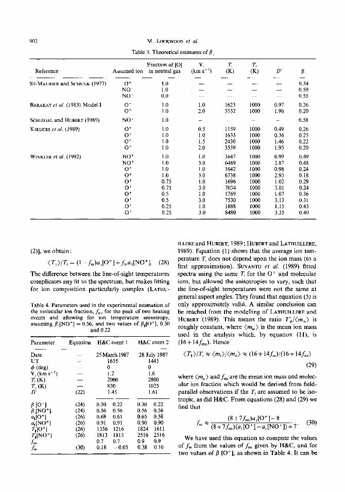
We now consider the effect of the anisotropy on the composition estimates by H&C. These authors made no allowance for temperature anisotropy, and hence effectively assumed a,, = 1. (Note that this does not apply to WEA because they observed at the aspect angle of 54.7”, for which a = 1 for both ion species.) In Table 4 we adopt values for &[O’] of 0.22 and 0.3. Inspection of Table 2 shows that half of the 24 observed B,, values (for assumed O+ ions) fall within this range, only three of the values being < 0.22. The remaining values exceed 0.3, but this may well indicate the presence of a significant proportion of NO+ ions. The most advanced of the theoretical simulations summarised in Table 3 is by WINKLER et al. (1992), who used a fully consistent ion-neutral collision model. The adopted range for &[O+] is consistent with nearly all their values, provided the neutral gas is at least 50% atomic oxygen.

In both cases we take /&[NO+] = 0.56, as derived

theoretically by SCHIZGAL and HUBERT (1989) and experimentally by LATHUILLERE et af. (199 1). However, we note that WINKLER et al. (1992) predict slightly smaller values, as shown in Table 3. However, these are derived for a neutral gas of pure atomic oxygen, and are expected to be increased by the presence of neutral molecules. In addition, ion-ion collisions also tend to increase &[NO+], so there may be no discrepancy between the predictions of Winkler et al. and the observations of Lathuillere et al. In this paper we adopt the value B,,[NO+] = 0.56 reported observationally, but note that it may not be consistent with the full rAnge of values of &[O+].

For a mixture of ions we can define the line-of- sight temperature at a general aspect angle 4 to be (LATHUILLERE and HUBERT, 1989) :

CT,> = (1 -fm)~,[O+l+fmT~[NO+l. (27)

If we apply this equation to the field-aligned direction 4 = 0” and insert the a,, (= T,,/T,) factors [equation


Table 3. Theoretical estimates of fi,,

Reference Fraction of [0] Y

Assumed ion in neutral gas (km s- ‘)

ST-MAURICE and SCHUNK (1977) 0+ 1.0 NO+ 1.0 NO+ 0.0

BARAKAT et al. (1983) Model I 0+ 0+

1.0 1.0

SCHIZGAL and HUBERT (1989)

KIKUCHI et al. (1989)

NO+

0+ 0+ Of 0+

1.0

1.0 1.0 1.0 1.0

WINKLER et al. (1992) NO+ NO+ Of 0+ 0+

g:

Of 0+ 0+

1.0 1.0 1.0 1.0 0.75 0.75 0.5 0.5 0.25 0.25

1.0

2.0

0.5 1.0 1.5 2.0

1.0 3.0 1.0 3.0 1.0 3.0 1.0 3.0 1.0 3.0

1623 3532

1159 1635 2430 3539

1647 6489 1642 6738 1696 7034 1769 7530 1888 8480

0.34 0.59 0.55

1000 0.97 0.26 1000 1.96 0.20

0.58

1000 0.49 0.26 1000 0.36 0.25 1000 1.46 0.22 1000 1.95 0.20

1000 0.99 0.49 1000 2.87 0.48 1000 0.98 0.24 1000 2.93 0.18 1000 1.02 0.29 1000 3.01 0.24 1000 1.07 0.36 1000 3.13 0.31 1000 1.15 0.43 1000 3.35 0.40

(2)], we obtain :

(~,,>/T, = (1-f,)a,,[0+l+f,a,,[NO+l. (28)

The difference between the line-of-sight temperatures

complicates any fit to the spectrum, but makes fitting

for ion composition particularly complex (LATHU-

Table 4. Parameters used in the experimental estimation of the molecular ion fraction, f,,, for the peak of two heating events and allowing for ion temperature anisotropy, assuming &[NO+] = 0.56, and two values of j,,[O’], 0.30

and 0.22

Parameter Equation H&C event 1 H&C event 2

Date 25 March 1987 28 July 1987 YTdcg) 0 1655 0 1445

V, (km s- ‘) 1.2 1.6 T, (K) 2000 2800 T, (W 830 1025 D' (22) 1.45 1.61

B,,IO’l ;;:; 0.30 0.22 0.30 0.22 B,,[NO+l 0.56 0.56 0.56 0.56 aIIP+l (26) 0.68 0.61 0.65 0.58 al,[NO+l (26) 0.91 0.91 0.90 0.90 T,,P+l (26) 1356 1216 1824 1611 T,,[NO+l (26) 1813 1813 2516 2516 f,, 0.7 0.7 0.9 0.9 fm (30) 0.18 -0.05 0.38 0.10

ILLERE and HUBERT, 1989 ; HUBERT and LATHUILLERE,

1989). Equation (1) shows that the average ion tem-

perature T, does not depend upon the ion mass (to a

first approximation). SUVANTO et al. (1989) fitted

spectra using the same T, for the Of and molecular

ions, but allowed the anisotropies to vary, such that

the line-of-sight temperatures were not the same at

general aspect angles. They found that equation (5) is

only approximately valid. A similar conclusion can

be reached from the modelling of LATHUILLERE and

HUBERT (1989). This means the ratio T;/(Q) is

roughly constant, where (m,,) is the mean ion mass

used in the analysis which, by equation (II), is

(16+ 14fmJ. Hence

(r,,>/T z (mi>/(mii> x (16+14fm)/(l6+14&)

(29)

where (mi,) and fmi are the mean ion mass and molec-

ular ion fraction which would be derived from field-

parallel observations if the T, are assumed to be iso-

tropic, as did H&C. From equations (28) and (29) we

find that

(8 +7fmi)a\l IO+] - 8

We have used this equation to compute the values

of fm from the values of fmi given by H&C, and for

two values of &[O+], as shown in Table 4. It can be


seen that, for b,,[O+] = 0.3 as used in Table 4, the derived molecular ion fraction is considerably smaller when allowance is made for the anisotropies ; for event 1 it is reduced from 70 to 18 % , for event 2 it is reduced from 90 to 38%. These values are still considerably greater than the values computed from chemical equilibrium, as given in Table 1 (4% for event 1 and 16% for event 2). Table 4 shows how sensitive is the value off, to the adopted &[O+]. For H&C’s event 1, the lower value of 0.22 results in a small, negativef,. This means that the observed line-of-sight temperature rose by more than we would predict for the observed ion flows, and hence the inferred mean ion mass falls below 16 a.m.u. This is obviously incorrect and implies that /.,,[O+] is greater than 0.22 for this event. Given that the ion drift is quite low (D’ = 1.45), this is not surprising. For the event 2, D’ is 1.6, and hence p,,[O+] may be somewhat lower than for event 1. Table 4 shows that, for &[O+] = 0.22, the 90% fraction of molecular ions inferred by H&C falls to lo%, which is lower than computed for chemical equilibrium.

H&C estimate that for their event 2, fm only decreases from 90 to 75% if a correction is made for non-Maxwellian effects. They do not give details of this calculation, which gives a much larger fm than our calculations for non-Maxwellian effects and for chemical equilibrium (Tables 1 and 4).

4. DISCUSSION OF ANISOTROPY MEASUREMENTS

HBggstrijm and Collis point out that the presence of molecular ions affects the analysis of non-Maxwellian plasmas. It is therefore instructive to examine the effects of molecular ions on anisotropy measurements made by EISCAT, for which in most cases a pure Of ion gas has been assumed. These measurements have been made using one of four techniques.

4.1. Tristatic observations at a single point (PERRAUT et al., 1984; LBVHAUG and FL& 1986; GLATTHOR and HERN~NDEZ, 1990)

In these cases, the temperatures derived from spectra observed at three different aspect angles 4 are compared. All three spectra should be influenced to the same extent by the presence of molecular ions. Hence the three derived temperatures would be underestimated by the same factor and no spurious anisotropy would be introduced. In fact, because the molecular ions would be less anisotropic (unless they are rare NT ions-see WINSER et al., 1989) this technique would underestimate the anisotropy of the O+ ions if molecular ions were present but neglected.

4.2. Observations at a range ofpoints (LOCKWOOD and WINSER, 1988)

This is very similar to the first method, except that to get a larger range of aspect angles, 4, it is assumed that the neutral thermosphere is spatially uniform over about 5” of latitude. Only scans in which the measured plasma drift is roughly constant at all scattering volumes have been analysed by this method. The anisotropy could be introduced here if there were more molecular ions at the larger 4 scattering volumes. Otherwise the arguments are as for the first method.

4.3. Observations of non-Maxwellian distortion of the spectrum at large 4 (LOCKWOOD et al., 1989 ; SUVANTO et al., 1989)

This method fits a non-Maxwellian distortion factor (D*) to the observed spectrum and then relates this to the anisotropy by employing a mode1 (semi- empirical) of the ion velocity distribution function. For the RAMAN et al. (1981) mode1 used, the anisotropy is in fact T,/T,, = (1+ D*‘). SUVANTO et al. (1989) and WINSER et al. (1989) have shown that the O+ gas is more highly non-Maxwellian than would be deduced if the molecular ion fraction were underestimated, that is, the D* and the anisotropy would also be underestimated.

4.4. Comparison ofjeld-aligned temperature rises with the predicted three-dimensional temperature rise from the frictional heating equation (MCCREA et al., 1992)

This method is essentially that used by HlggstrGm and Collis except that, whereas H&C assume the anisotropy and derive the composition, McCrea et al. assume the ion composition and derive the anisotropy. In this one case, therefore, the anisotropy will be overestimated if the mean ion mass is underestimated. However, we have shown in this paper that the relatively small change from 0.22 to 0.3 (i.e. 36%) in the assumed anisotropy factor, p,,[O+], causes a factor of 4 change in the derived fraction of molecular ions (see Table 4): conversely, large changes in the assumed ion composition will cause relatively small errors in the derived anisotropy.

4.5. Uncertainties in the determination of ion composition and anisotropy

To investigate these effects for this fourth method in further detail, let us consider photochemical equilibrium, as would apply in the daytime lower F-layer. The plasma density is then given by (RISHBETH and


GARRIOTT, 1969, section 3.6 1) :

Ne = (qPP){l + 11 + (4Pzl~q)l I’*). (31)

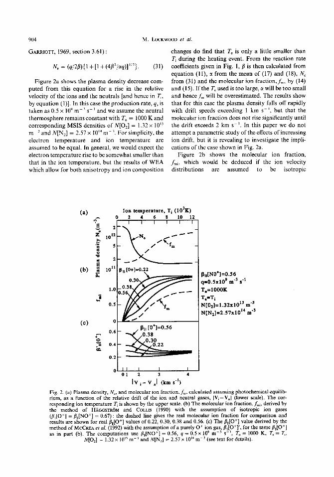
Figure 2a shows the plasma density decrease computed from this equation for a rise in the relative velocity of the ions and the neutrals [and hence in T,, by equation (l)]. In this case the production rate, q, is taken as 0.5 x 10’ mm 3 s- ’ and we assume the neutral thermosphere remains constant with T, = 1000 K and corresponding MSIS densities of N[O,] = 1.32 x lOI m _ 3 and N[N,] = 2.57 x lOI m- 3. For simplicity, the electron temperature and ion temperature are assumed to be equal. In general, we would expect the electron temperature rise to be somewhat smaller than that in the ion temperature, but the results of WEA which allow for both anisotropy and ion composition

changes do find that T, is only a little smaller than T, during the heating event. From the reaction rate coefficients given in Fig. 1, fi is then calculated from equation (ll), c( from the mean of (17) and (18), N, from (31) and the molecular ion fraction,&, by (14) and (15). If the T, used is too large, LX will be too small and hence fm will be overestimated. The results show that for this case the plasma density falls off rapidly with drift speeds exceeding 1 km s- ‘, but that the molecular ion fraction does not rise significantly until the drift exceeds 2 km s- ‘. In this paper we do not attempt a parametric study of the effects of increasing ion drift, but it is revealing to investigate the impli- cations of the case shown in Fig. 2a.

Figure 2b shows the molecular ion fraction, fmi, which would be deduced if the ion velocity distributions are assumed to be isotropic

(a)

(cl

Ion temperature, Ti (103K) 0 2 4 6 8 10 12

I I I I I I( 2 \

0.6

0.4

0.2

&,[NO+]=0.56 q=0.5x109 mm3 s-l T,=lOOOK

T.=Ti

N[02]=1.32x10” me3

N[N+2.57x10L4 mm3

hi-Vni (kms-‘)

Fig. 2. (a) Plasma density, N,, and molecular ion fraction, f,, calculated assuming photochemical equilibrium, as a function of the relative drift of the ion and neutral gases, IV,-V,( (lower scale). The corresponding ion temperature T, is shown by the upper scale. (b) The molecular ion fraction, fm,, derived by the method of H&GSTR~M and COLLIS (1990) with the assumption of isotropic ion gases (&[O’] = &[NO+] = 0.67) : the dashed line gives the real molecular ion fraction for comparison and results are shown for real &[O’] values of 0.22, 0.30, 0.38 and 0.56. (c) The &[O’] value derived by the method of McCRE.4 ef al. (1992) with the assumption of a purely Of ion gas, &[O’]‘, for the same &[O’] as in part (b). The computations use &[NO*] = 0.56, 4 = 0.5 x lo9 mm3 s-‘, T, = 1000 K, T, = T,,

N[O,] = 1.32 x IO” mm3 and MN,] = 2.57 x lOI mm3 (see text for details).


(/l,,[O+] = p,,Ir\rO’] = 0.67), using the method of H&C. These curves are calculated using equation (29). Because we do not know exactly how &[O’] varies with the relative ion drift, we here show the results for a range of fixed values (0.22, 0.3, 0.38 and 0.56): P,,[NO+] is taken to be 0.56 for all cases. The dashed line shows the real molecular ion fraction. Even for small ion drifts. the derived composition is seriously in error, and the error increases rapidly with decreasing &[O*]. In practice, we may expect &[O ‘1 to decrease with increasing drift (MCCREA et al., 1992). Figure 2b shows how extreme the composition errors can be. LOCKWOOD and WINSER (1988) derived fl,,[O’] of 0.22 for a drift of 2 km s- ‘, for which we here compute a real molecular ion fraction of about 0.1, whereas assuming isotropy gives a vaiue of 1. I, that is, a mean ion mass of 33 a.m.u.

Figure 2c shows the values for /?,,[O’] which would be derived by the method of MCCREA et al. (1992), and assuming that only O+ ions are present: we denote this value as @,,[O’]‘. As expected, the method underestimates &[O’] as the molecular ion fraction increases. The largest errors are 4.5, 17, 26 and 48% for real &[O+] values of 0.22, 0.3, 0.38 and 0.56, respectively. Given that all theoretical estimates of p,,[O+] are generally below about 0.38, this puts a likely upper limit on the error of about 26%. This error occurs for an ion drift above 3 km s ‘. In general, McCrea et al. only used data with ion drifts below about 1.5 km s- ‘, so for the case shown in Fig. 2, the assumption of pure O+ would only cause errors of 2.5, 3.5 and 4% for real &[O’] values of 0.22, 0.3 and 0.38.

There are many reasons why the & factors vary, including variations in the neutral densities, the relative ion-neutral drift speeds and the ion-ion collision frequency (MCCREA et al., 1992; WINKLER et al.,

1992). However, it is now clear that all four of the above methods give somewhat similar results and the anisotropy of the ion gas cannot be ignored during ion heating events, unless the observations are made at the special aspect angle of 54.7’.

We have re-evaluated the calculations of the expected molecular ion content of the lower F-region made by WINSER et al. (1990). Using the ion temperature which allows for the ion composition change (i.e. that computed from the ion energy balance equation) and realistic reaction rate coefficients, we find that chemical equilibrium can explain a dominance of

molecular ions (the fraction of molecular ions predicted here is 90%% ciose to the 100% derived from the data). The remaining difference is probably due to underestimation of the neutral densities and/or departures from chemical equilibrium. The higher reaction rates used here also give the observed time constant for the increase of the molecular ion fraction. These results are consistent with the recent modelling of the effects of rapid flows in sub-aurora1 ion drift events (SELLEK er al., 1991 ; MOFFETT et al., 1992).

However, chemical equilibrium predicts molecular ion percentages which are an order of magnitude smaller than derived by H;~GGSTR~~M and COLLIS (1990). Use of self-consistent electron temperatures would lower the predicted values still further. These authors do not consider in detail the effects of anisotropic ion velocity distributions which would cause them to overestimate the molecular ion fraction. Using the lowest of the values for the ‘parallel temperature partition coefficient’ for 0’ ions, &[O+], we find here that the ion gas would only have changed to a low (<9%) fraction of molecular ions. If &[O+] is larger, the molecular ion fraction in the heating event would be greater than this. However, realistic /l,[O+] values still give much smaller molecular ion fractions than are derived with the assumption of isotropy. The large molecular ion content derived by Winser et al.

is not subject to this effect because these authors employed the special aspect angle of 54.7”. However, the plasma drifts in the case studied by Winser et al.

were 3 km s- ‘, twice that in the larger of the two events studied by Haggstriim and Collis.

We have also studied the sensitivity to variations in the ion composition of the method used by MCCREA et al. (1992) to study the anisotropy of the O+ gas. It is shown that the anisotropy is overestimated (&[O+] is too low) if molecular ions are neglected, but that for the range of &JO’] predicted theoretically, the error is reasonably smail (below about 25%). Furthermore, if only low drift speeds are employed, the error is even smaller : for the one example described here, errors are below 5% for ion drifts not exceeding 1.5 kms’.

Acknowle~e~nzs-me work at Sheffield and South- ampton was supported by S.E.R.C. grants GR/G 05087 and GR/E 73956, respectively. We thank K. J. Winser for useful discussions. The EISCAT Scientific Association is supported by the Suomen Akatemia of Finland, the Centre Nationale de la Recherche Scientihque of France, the Max-Planck Gesellschaft of Germany, the Norges Ahnenvitenskaplige Forskningsr~d of Norway, the Natu~etenskapliga Forsk- ningsradet of Sweden. and the Science and Engineering Research Council of the U.K.

YO6 M. LOCKWWD et al.

REFERENCES

BAILEY G. J. and SELLEK R. BARAKAT A. R., SCHUNK R. W. and ST-MAURICE J.-P GLATTHOR N. and HERNANDEZ R. H~~GGSTR~~M I. and COLLIS P. N. HEDIN A. E. HUBERT D. HUBERT D. and LATHUILLERE C. KIKUCHI K., ST-MAURICE J.-P. and BARAKAT A. R. LATHUILLERE C. and HUBERT D. LATHUILLERE C., HUBERT D., LA Hoz C. and

KOFMAN W. LOCKWOOD M., BROMAGE B. J. I., HORNE R. B.,

ST-MAURICE J.-P., WILLIS D. M. and COWLEY S. W. H.

LOCKWOOD M., SUVANTO K., ST-MAURICE J.-P., KIKUCHI K., BROMAGE B. J. I., WILLIS D. M., CROTHERS S. R.. TODD H. and COWLEY S. W. H.

LOCKWOOD M., SUVANTO K., W~NSER K. J.. COWLEY S. W. H. and WILLIS D. M.

LOCKWOOD M. and WINSER K. J. LWHAUG U.-P. and FLA T. MCCREA I. W., LESTER M., ROBIN~QN T. R.,

ST-MAURICE J.-P., WADE N. M. and JONES T. B. MOFFETT R. J., HEELIS R. A., SELLEK R.

and BAILEY G. J. M~~RCROFT D. and SCHLEGEL K. PERRAUT S., BREKKE A., BARON M. and HUBERT D. RAMAN R. S. V., ST-MAURICE J.-P. and ONG R. S. B. R!ZES M. H.

RISHBETH H., BAUER P. and HANSON W. B. RISHBETH H. and GARRIOTT 0. K.

RISHBETH H., SMITH P. R., COWLEY S. W. H., WILLIS D. M., VAN EYKEN A. P., BROMAGE B. J. I. and CROTHERS S. R.

1989

1988 1986 1992

1992

1988 1984 1981 1989

1972 1969

1985

SCHIZGAL B. and HUBERT D. 1989

SELLEK R., BAILEY G. J., MOFFETT R. J., HEELIS R. A. and ANDERSON P. C.

ST-MAURICE J.-P. and HANSON W. B. ST-MAURICE J.-P., HANSON W. B. and

WALKER J. C. G. ST-MAURICE J.-P. and SCHUNK R. W. ST-MAURICE J.-P. and SCHUNK R. W. ST-MAURICE J.-P. and TORR D. G. SUVANTO K., LOCKWOOD M., WINSER K. J.,

BROMAGE B. J. I. and FARMER A. D. TERESHCHENKO V. D., TERESHCHENKO E. A.

and KOHL H. TORR D. G. and TORR M. R. WINKLER E., ST-MAURICE J. P. and BARAKAT A. R. WINSER K. J.. FARMER A. D.. REES D. and

ARUL~AH A. WINSER K. J., LOCKWWD M. and JONES G. 0. L. WINSER K. J., LOCKW~~D M., JONES G. 0. L.,

RISHBETH H. and ASHF~RD M. G. WINSER K. J., LOCKW~~D M., JONES G. 0. L.

and SUVANTO K.

1990 Ann. Geophys. 8, 17 1. 1983 J. geophys. Res. 88,323l. 1990 J. atrnos. terr. Phys. 52, 545. 1990 J. atmos. terr. Phys. 52, 519. 1987 J. geophys. Res. 92,4649. 1984 J. atmos. terr. Phys. 46,601. 1989 J. geophys. Res. 94, 3653. 1989 Ann. Geophys. I, 183. 1989 Ann. Geophys. I, 285. 1991 Geophys. Res. Lett. 18, 163.

1987 Geophys. Res. Lett. 14, 111.

1988 J. atmos. terr. Phys. 50,467.

Adt. Space Res. 9(5), 113.

Planet. Space Sci. 36, 1295. J. atmos. terr. Phys. 48, 959. J. ycophw. Res. (in press).

Planet. Space Sci. 40, 663.

J. atmos. terr. Phys. 50,455. J. atmos. terr. Phys. 46, 531. J. geophys. Res. 86,415 1. Physics and Chemistry of the Upper Atmosphere, Appen-

dix 5.1. Cambridge University Press, Cambridge. Planet. Space Sci. 20, 1287. Introduction to Ionospheric Physics. Academic Press,

New York. Nature 318,45 1.

Non-equilibrium nature of ion distribution functions in the high-latitude aurora1 ionosphere. RareJied Gas Dynumic.c: Space Related Studies. E. P. MUNTZ. D. P. WEAVER and D. H. CAMPBELL (eds), Progress in Astronautics and Aeronautics, Vol. 116. AIAA, Washington D.C.

1991 J. atmos. terr. Phys. 53, 557.

1982 J. geophys. Res. 87, 7580. 1976 J. geophys. Res. 81, 5438.

Planet. Space Sci. 25,243. Reu. Geophys. Space Phys. 18,813. J. geophys. Res. 83, 969. J. atmos. terr. Phys. 51, 483.

1991 J. geophys. Res. 96, 17,591.

1979 J. atmos. terr. Phys. 41, 797. 1992 J. geophys. Res. 97, 8399. 1988 J. atmos. terr. Phys. 50, 369.

1987 Geophys. Res. Lett. 14,957. 1990 J. atmos. terr. Phys. 52, 501.

1989 J. geophys. Res. 94, 1439.

eiscat observations of ion composition and temperature anisotropy in the high-latitude f-region

Documents