eiscat incoherent scatter radar observations and model studies of day to twilight variations in the...

Journal q/ Almosphrrrc and Twrestrtul Phyxcs, Vol. 55, No. 4iS. pp. 767-781, 1993. 0021--9169/93 $b.oO+ .XI Printed in Great Britain. (?-- 1993 Pergamon Press Ltd

EISCAT incoherent scatter radar observations and model studies of day to twilight variations in the D-region during the PCA event

of August 1989

E. TURUNEN

Sodankyla Geophysical Observatory, SF-99600 SodankylB, Finland

(Receiz$ed in,final,form 17 February 1992 ; ucceped 2 June 1992)

Abstract-An intense solar proton event causing enhanced ionization in the ionospheric R-region occurred on 12 August 1989. The event was partially observed during three successive nights by the EISCAT UHF incoherent scatter radar at Ramfjordmoen near Tromso, Norway. Ion production rates calculated from GOES-7 satellite measurements of proton flux and a detailed ion chemistry model of the D-region are used together with the radar data to deduce electron concentration, negative ion to electron concentration ratio, mean ion mass and neutral temperature in the height region from 70 to 90 km, at selected times which correspond to the maximum and minimum solar elevations occurring during the radar observations. The quantitative interpretation of EISCAT data as physical parameters is discussed. The obtained temperature values are compared with nearly simultaneous temperature measurements at Andsya based on lidar technique.

1. INTRODU~ION

The incoherent scatter technique has been widely used to study the lowest part of the ionosphere. The pion- eering work in this field was mostly done in Arecibo (see reviews by MATHEWS, 19X1, 1984), where the instrumental configuration is well suited for D-region work. For the EISCAT UHF and VHF radars, soph- isticated experiment algorithms and corresponding analysis methods have been developed to overcome the limitations in data interpretation due to weak D- region signals (TUR~NEN, 1986 ; POLLARI et al., 1989 ; LA Hoz ef al., 1989). Measurement principles and experimental results from ElSCAT radars are reviewed by COLLIS and R~TTGER (I 990).

Data analysis can be based on theoretical work originating from e.g. DOUGHERTY and FARLEY (1963), TANENBAUM (1968), MATHEWS (1978) and FUKUYAMA and KOFMAN (1980). Simple expressions arise in the first approximation, relating physical parameters like ion velocity, electron concentration, temperature, mean ion mass, ion-neutral collision frequency and negative ion concentration, to the Doppler shift, power and spectral width of the scattered signal. Although there is some evidence (HANSEN et al., 1991) for lack of accuracy in the most commonly adopted approximations (see Section 4), the results derived using them show similar features as those obtained by other techniques. The best established parameters are electron density and ion velocity, for which com- parisons with other measurement techniques are readily available (e.g. MATHEWS et al., 1981 ; HALL et

al,, 198.5; RANTA et al., 1985 ; MEYER et al., 1987) and which appear to be easier to determine accurateiy. The results for negative ions, ion mass and temperature however suffer from inaccuracies. Firstly, the main effect of all these quantities is hidden in the same measured parameter, the spectral width. Secondly, a very weak signal makes a reliable spectral width estimation difficult without a long time integration of the raw data. The traditional solution to these problems is to use empirical models or independent measurements for selected physical parameters. This is aIso what is needed in accurate electron density estimates, if the raw electron density, derived from backscattered power, is to be corrected for finite electron Debye length effects, using the algorithm described by MATHEWS et al. (1982). Alternatively, it is possible to add in the data interpretation a priori

information of atmospheric behaviour, that is, neutral scale height may be extracted from the altitude variation of spectral width data (TEPLEY and MATHEWS, 1978).

Under conditions of high D-region ionization, the incoherent scatter signal strengthens and the spectral width estimation becomes practical. For the EISCAT UHF radar this happens during high energy electron precipitation (TURUNEN et al., 1988 ; HALL et al.,

1988) or during solar proton events, which cause the polar cap absorption (PCA) phenomenon (HAR- GREAVES et al., 1987; COLLIS and RIETVELD, 1990). Estimates of negative ion to electron concentration ratio using EJSCAT radars have been presented by KOFMAN er al. (I 984) and HALL ef al. (1987, 1988).

768 E. TURUNEN

POLLARI et al. (1989) showed, using sample spectral width data, how a very detailed experiment algorithm

treatment is necessary in reliable data analysis of Barker coded experiments. Kofman et al. used a bistatic radar experiment configuration and thus could reduce unwanted signal contribution in the data. However, the signal was noisy and the negative ion information was highly scattered. Hall et al. applied initially fixed height profiles of ion mass and independent information on temperature.

This paper introduces a complementary interpretation of incoherent scatter data from the D-region. Physical parameters electron concentration, negative ion to electron concentration ratio, mean ion mass and neutral temperature are estimated simultaneously from theoretical expressions of scattered signal power and spectral width. Ion velocity is not treated in this context, since its effect is only to cause Doppler shift to the scattered signal. This effect is removed in the first step of data analysis, where a Lorentzian spectrum form is fitted to the signal. The data interpretation is accomplished via the use of a detailed ion chemistry scheme, which needs as extra input the neu-

tral atmosphere composition and primary ion production rates. This interpretation is done to the EISCAT data obtained during the first three nights of the PCA event of 12 August 1989. The ion production is calculated from GOES-7 satellite measurements of

proton flux in the solar wind. When all the involved equations are treated in a consistent way, we are able to estimate the four unknown physical parameters.

2. THE POLAR CAP ABSORPTION EVENT OF

12 AUGUST 1989

The solar proton event starting on 12 August 1989, was seen by riometers as a PCA event lasting for

nearly two weeks. The riometer observations during the PCA are described in detail by RANTA et al. (1992). Figure 1 shows an example of 30 MHz riometer data recorded in Abisko (68.4”N, 18.9”E) on 12-15 August 1989. Maximum absorption due to proton flux induced high ionization in the D-region was 16 dB. After the onset of the event, distinct minima in absorption are seen to occur during all three nights. This time variation is expected to be due to negative ion formation and consequent free electron loss, in the absence of direct sunlight. Although absolute night conditions are not reached at D-region heights in the middle of August at the latitude of Abisko, the absorption data suggest that negative ion formation by electron attachment to neutrals is prevailing. The part of solar spectrum which is responsible for elec-

Absorption [dB] Sun elevation

m EISCAT exprlment

Time UT

Fig. 1. Polar Cap Absorption event as seen by 30 MHz riometer in Abisko during 12-15 August 1989. The solid line indicates observed absorption. Solar elevation angle is also plotted as the dashed line. EISCAT D-region experiment

times are denoted by the shaded regions.

tron detachment from negative ions, is absorbed in

the lower atmosphere. The overall daytime time variation is expected to

reflect changes of the proton flux penetrating in the atmosphere. Assuming this flux to be known from

measurements in the solar wind, one is able to calculate the primary ion production rate due to protons,

if neutral atmosphere density and composition are known. Figure 2 shows the proton flux data from six energy channels, recorded on board satellite GOES-7 (SOLAR GEOPHYSICAL DATA, 1989) during the same

interval as shown in Fig. 1. During the first night, the flux increases at all energies and the flux of highest energy protons reaches its maximum. The flux of low energy protons is highest during the second night at around 0300 UT. Towards the third night, the fluxes steadily decrease at all channels. In addition to the above described time variations, the absorption data of Fig. 1 contain a sharp minimum on 14 August at 0800 UT. We do not discuss this feature further, but mention only that it is probably connected with the

sudden storm commencement occurring at that time (RANTA et al., 1992) and could possibly be interpreted as effective increase in cut-off rigidity for the protons (see HULTQVIST, 1963).

Qualitatively, the process of negative ion formation

has been known to be the reason of day to night variation in absorption data during PCA events (HULTQVIST, 1963). In the following we want to take a more quantitative look at this special PCA event. We try to answer the following question : exactly how many negative ions are formed during the night-time in the height region which we are able to investigate with the EISCAT radar and to what degree do we understand this process theoretically? A simple estimate, which could be based on the assumption that

Day to twilight variations in the D-region 769

all free electrons disappearing in the night are forming negative ions, is not satisfactory since effective recombination rate of electrons is also changing from day to night. As a starting point to the estimates presented in Sections 4 and 5, the ion production rates due to protons are calculated from the data presented in Fig. 2. The algorithm for this calculation is originally due to Reid and was used in the study of the PCA event of February 1984 by HARGREAVES et al. (1987). The only difference in the calculation is that now we select the MSIS-86 model, extrapolated below mesopause as described by ALCAYD~ (1981), to represent the neutral atmosphere and we use 1 km altitude steps. At this stage the temperature is also taken from the model, but later, when solving for the physical parameters from EISCAT data, temperature is taken to be an independent unknown variable.

The result of ion production rate calculation, in the height range from 70 to 90 km, is given in Fig. 3. This height range matches the altitude coverage of EISCAT spectral width data which is discussed in Section 3. We see that in the beginning of the proton event the maximum ion production takes place below 70 km. Later during the second night we start to see the maximum production in our selected height range. Finally during the third night of the event, when the level of production has substantially decreased, we are covering all important excess ionization with EISCAT data. The time variation of total integrated ion production, in the height range from 70 to 90 km, can be said to resemble the time variation of riometer absorption, shown in Fig. 1, if one notes that in the first part of the event we are missing an important part

of ion production which is effective for the measured absorption.

3. EISCAT OBSERVATIONS

The incoherent scatter data presented in this work were recorded with the EISCAT UHF radar system (FOLKESTAD et al., 1983) at Ramfjordmoen, Norway using the special D-region experiment algorithm GEN-11. This experiment is described by TURUNEN (1986), and the related modulation effects and raw data analysis features are explained in detail by POL- LARI et al. (1989). We note here only that the range gate separation is 1.05 km, basic time resolution is 10 s and useful spectral width data from the UHF radar, with vertical antenna position, are received in altitude range from 70 to 90 km. The EISCAT observations during the period 12-15 August 1989, were part of a larger campaign to study the polar meso- spheric summer echoes. The antenna pointing geometry was chosen to include four antenna pos- itions: vertical, to the south, vertical, to the west. Measurement in each position lasted for 5 min. Thus a natural post-integration time of 5 min gives a time resolution of 10 min in the vertical antenna position which is used in this study. Observations were made from 3 to 15 August in periods of 6-9 h each night, centred on local midnight. The EISCAT observation times during the PCA event are denoted in Fig. 1. The solar elevation angle is also shown in Fig. 1, to illustrate the coverage of solar illumination conditions present in the radar data. The maximum and minimum elevation angles during radar measurements are

lo4 I

in-4

I

F 4.2-6.7 MeV W-W-SeMv”V

39-sZ MeV

‘“20.00 06.06 16.00 02.06 12.00 22.00 UT

Time

Fig. 2. Proton Anxes in solar wind measured by the satellite GOES-7 during the three nights shown in Fig. 1 (from SOLAR GEOPHYSICAL DATA, 1989). Continuous lines are drawn during EISCAT observation times.

770 E. ?bUJNEN

+9 and - 6”, respectively. Thus we have measurements during the daytime and twilight conditions, but absolute darkness is not reached in the D-region.

Radar data analysis is divided into two phases. First, a raw data analysis is performed as described by POLLARI et al. (1989). In this step, range ambiguity effects are removed from data and a Lorentzian fit with varying number of parameters is done, to extract an estimate of scattered signal power and spectral width due to ion line contribution. The fit is supposed to remove ground clutter from the lowest measured altitudes, as well as the electron line contribution in the signal. The fit also gives an estimate of the neutral wind component along the antenna beam direction, but this parameter will not be discussed further here. A raw electron density estimate is formed from the scattered power, with the assumption of thermal equilibrium between electrons and ions, absence of negative ions and neglecting the electron Debye length effects. This estimate is based on the radar equation

(1)

where Csrs is the radar system constant, kB the Boltz- mann constant, T,, the calibration temperature, bw the filter bandwidth, r the distance from radar to the scattering volume, P, the transmitted power, 7 the pulse length, P,, the received power estimate, PC,, the calibration power and Pbac the background power. In the second step of data analysis, interpretation of the raw radar data as physical parameters electron density, mean ion mass, temperature and negative ion to electron concentration ratio is done. This analysis includes the use of a specific ion chemistry model. The procedure is described in detail in Section 4.

The result of raw data analysis is shown as Fig. 4. The upper panel represents the time variations of raw electron density and the corresponding spectral width is given in the lower panel. The time axis in this figure is composed piecewise, to show only the three nights of EISCAT experiments. At the lowest altitudes, the time variation of spectral width is seen to anticorrelate with that of the raw electron density. When the electron density decreases during each night, the spectral width increases at the same time. Both the electron density decrease (as discussed in Section 2) and the spectral width increase (see e.g. MATHEWS, 1978) are signatures of negative ion formation below 80 km during night-time. A simple estimate of negative ion concentration would be possible if all lost electrons were assumed to form negative ions (COLLIS and RIET- VELD, 1990). However, the effective recombination is expected to change during night and thus a more detailed treatment of negative ions is necessary. We

have selected two representative times of midnight and daytime conditions for further analysis from the night of 13-14 August, since during this night the radar signal was strongest and consequently the spectral width data appear noiseless. The selected times are 0005 and 0255 UT, corresponding to solar zenith angles 95 and 86”, respectively.

4. INTERPRETATION OF EISCAT DATA

When raw electron density NFw and spectral width A.w, assuming a Lorentzian shape, have been deduced in the first step of radar data analysis, we can relate these two parameters to physical quantities--electron concentration N,, temperature T, mean ion mass mi, ion-neutral collision frequency vin and negative ion to electron concentration ratio 1 via expressions (FUKU- YAMA and KOFMAN, 1980; MATHEWS, 1978) :

where 1, is the radar wavelength. Here we have assumed thermal equilibrium of all species. In addition, it is assumed that the product of ion mass and collision frequency, m,vi,,, is equal for positive and negative ions. If the ion-neutral collision frequency is further related to neutral density, as given, for example, by BANKS and KOCKARTS (1973), we have in expressions (2) and (3) two known measured parameters and four unknown quantities to be deduced, supposing that the neutral atmosphere is given.

The amount of independent unknown parameters can be reduced, if we are able to add new relations between them, as described by an ion chemical model scheme, appropriate for the D-region. A strict mathematical solution would then need two independent new relations to be established. However, this is not a suitable approach to a physical problem, since we should care about the existence of a solution for a set of four nonlinear equations and we already have taken a lot of simplifying approximations in accepting expressions (2) and (3). A simple physical solution utilizing an ion chemical scheme is described below.

In expression (2) the terms including square roots describe the Debye length effect on scattered signal

772 E. TURUNEN

EISCAT Raw Electron Density

h.05 0335 h .05 04.i ho.35 01.5’5 12n3.08.89 13Il4.08.89 14fl5.08.89

Time UT

EISCAT Signal Spectral Width

800

500

300

200

100

iO.05 03.35 il.05 04.a io.35 01 .s5 12il3.08.89 13b4.08.89 Wl5.08.89

Time UT Fig. 4. EISCAT raw electron density (upper panel) and spectral width (lower panel) as functions of time

and altitude. The time axis is similar to that of Fig. 3.


power. Usually these terms are small, but they are not negligible in the lower D-region. If information on negative ion to electron concentration 1 and temperature T is available, expression (2) may be solved, to give a corrected electron density estimate. On the other hand, if electron density is approximated to some accuracy and ion mass m, is also known, expression (3) may be solved to give 1. Thus it seems likely that for some range of the physical parameter values, expressions (2) and (3) may the solved simultaneously, to give N, and 1, when m, and T are known and for some cases they may be used separ- ately. It turns out that an analytical solution of (2) and (3) exists if the ratio of the product of the first two multiplicative terms in expression (3) to the spectral width is less than one. The solution is explicitly written down in Appendix 1. This however includes also solutions, for which the value of 1 is negative, which happens at the altitudes where we normally expect 1 to be zero. At these altitudes we may set 1 equal to zero and calculate the Debye length correction to the raw electron density estimate from expression (2) only.

Mean ion mass is available through solution of a selected ion chemistry model. These models usually adopt a description of neutral atmosphere as input and give different ion concentrations as result, assuming ionizing factors are known. Since most chemical reactions are temperature dependent, we may select temperature as a free parameter to be adjusted, so that the model electron density and the one from corrected radar estimate agree to an acceptable accuracy. This results in an iterative procedure, where for each height we start with a temperature value and corresponding neutral atmosphere. Ion production rate is then calculated and the chemical equilibrium is solved to give ion concentrations and thus electron density, negative ion density and mean ion mass. Solution of expressions (2) and (3) is then compared for electron density and the temperature is changed accordingly to make the process converge. Note that neutral density is also changed, by integration from a reference point, according to temperature change and keeping the relative amounts of each neutral constituent in constant proportions. Thus all the above-mentioned steps are repeated for each iteration. If the model and the solution of expressions (2) and (3) are consistent, we also expect negative ion to electron density concentrations to be in agreement, at least in some height range. This check will serve as a justification of the use of expressions (2) and (3). Mathematically, if the neutral concentrations were adjusted, one could easily imagine a fit to almost any data, since we then would have as many degrees

of freedom available as we could wish to use. However, then we would be faced with the problem of choosing the preferable neutral parameters to be varied.

The selected ion chemistry model (SIC-model) is described by BURNS et al. (1991). The positive ions and their mutual reactions are shown in Fig. 5a and the negative ion scheme is presented in Fig. 5b. All involved chemical processes are not denoted in Fig. 5. The model also includes reactions due to recombination of positive ions with electrons, photodissociation of positive ions, electron photo- detachment of negative ions, photodissociation of negative ions, electron attachment to neutrals and ion-ion recombination. A complete reaction list is given by Burns et al. in their appendix 1. Photo- ionization is included in calculations, although the dominant ionization source in the present application is the proton flux, discussed in Section 2. Neutral atmosphere is taken from MSIS86 (HEDIN, 1987) and an extrapolation below mesopause is performed according to ALCAYDB (1981). Those minor con- stituents not covered by MSIS86 are selected to represent the conditions for zenith angles 86 and 95”, and are listed and plotted in Fig. 6. The night and daytime conditions are further separated by choosing reactions involving photons to be switched off during night-time.

5. RESULTS AND DISCUSSION

The initial conditions in solving the electron concentration, negative ion to electron concentration ratio, temperature and mean ion mass for the two selected times 0005 and 0255 UT on 14 August 1989, are illustrated in Fig. 7. The differences in the height profiles of raw electron density and spectral width during midnight and morning reflect the effect of negative ion formation, whereas the difference seen in ion production rates is due to changes in proton flux. At 0255 UT we see the maximum ion production in the measurement range of the radar, but at 0005 UT we are clearly missing an important part of ion production, due to the restricted altitude coverage of our data. However, this fact should not be mixed with the limitations when comparing the deduced electron density profile with riometer observations.

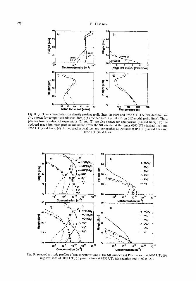
The deduced height profiles of electron density, negative ion to electron concentration ratio, temperature and mean ion mass are plotted in Fig. 8a, b, c and d, respectively. The raw electron density is also shown in Fig. 8a for comparison. The existence of negative ions at night-time has a considerable effect on scattered signal power. During daytime and also

E. TURUNEN

(4 N2, CO2

N2/ 0, I 0 I NO/ O$'Ad l e

03 0, - 202

0, 202 OZC’AS,

OZ,NZ 0

e

+n* f

Hco; . =02*2. * _ M l H/O

co; - CO2

CO202 .

COrN2 A

-Lr \) b

.I

, COro2 “CO2,02

A, N9 NO

v

NR NO

WY

0)) I

Fig. 5. (a) The positive ion reaction scheme in the adopted chemistry model (SIC-model, BURNS et al., 1991) ; (b) the negative ion reaction scheme in the adopted ion chemistry model (SIC-model, BURNS et al.,

1991).


72

70 lo3 10' 105 IO6 10' 108 109 Id'

Concentration [l/cm31

Fig. 6. Neutral minor constituent profiles in SIC-model not covered by MSIS86. They are selected to represent the times 0005 UT (dashed lines) and 0255 UT (solid lines) on 14 August 1989 corresponding to solar zenith angles 95 and 86”, respectively. Concentrations for CO, and H,O have been

calculated using fixed mixing ratios.

during night above 79 km, only the Debye length correction to raw electron density is effective. The value of this correction is of the order of 5-10%. At midnight, the negative ion to electron concentration ratio exceeds 1, below an altitude of 7.5 km. The value at the height of 70 km is 8. In the morning, a sign of negative ions appears only in the lowest measured gate at 70 km, the value of 3, being less than 1. In Fig.

8b the 1 profiles, drawn as solid lines, originate from the SIC-model. As a consistency check of the model and radar data, 3, profiles from solution of expressions

(2) and (3) are also shown as dashed lines. The different /z profiles do not quite agree, but they are consistent to an acceptable accuracy. The night-time value of 1 from this solution at 70 km is 6, which makes only a 25% difference to the SIC-model value.

The mean ion mass profiles in Fig. 8c differ mainly

for the negative ion region. This deviation is only

of the order of 10 a.m.u. and thus does not violate significantly our assumption of equal representative masses of negative and positive ions in expressions (2) and (3). The deduced temperature profiles in Fig. 8d are similar for midnight and morning times. The small differences, of the order of 5-15 K, correspond to small differences in ion mass profiles in the region with no negative ions.

Selected altitude profiles of ion concentrations in the SIC-model are plotted in Fig. 9a, b, c and d. The dominant positive ions are NO+ and 0: , competing at different altitudes. The concentrations of cluster ions are also competitive, but not strikingly abundant compared to the normal D-region situation where primary ion production rates are much less than in our case of a solar proton event. At altitudes higher than the actual negative ion region, the dominant negative ion is 0;. At night-time, this is replaced by the dominance of CO; and NO; below 75 km. At

daytime, HCO; also sets in at 70 km. The deduced electron density values can be checked

against riometer observations. Assuming electron- neutral collision frequency to be known, the integral absorption at 30 MHz along the radio wave path through the region measured by EISCAT can be calculated. Now we should note that especially during daytime, high ionization occurs below 70 km and consequently we would get too low values of absorption from EISCAT data. At night-time, however, the

free electrons are rapidly lost due to electron attachment to neutrals. Since absorption is only caused by

free electrons, we would be rather close to the observed absorption values at midnight. Figure 10 shows the comparison of observed and calculated absorption, for all three nights of EISCAT measurements. When solving expressions (2) and (3), we have used fixed averages of the deduced mean ion mass and temperature profiles, as if regarding the atmosphere

ii~ii_.xilK1 Id IO' IO'O 10" IW 200 300 400 5oQ 6W

Production rate [s%m3] Raw electron density [m-9 Spectral width [Hz]

Fig. 7. Altitude profiles of initial ion production rate, EISCAT raw electron density and spectral width at the times 0005 UT (dashed lines) and 0255 UT (solid lines) on 14 August 1989.

776 E. TURUNEN

70 109 10’0

Electron density [m-a] II

a --__ -. -85 E d ,

Eeo /pl

9

2 : 75

I;-:: ,’

\ \ ‘\

:

7o

30 hban”ion%asF[amZ]

Fig. 8. (a) The deduced electron density profiles (solid lines) at 0005 and 0255 UT. The raw densities are also shown for comparison (dashed lines) ; (b) the deduced I profiles from SIC-model (solid lines). The 1 profiles from solution of expressions (2) and (3) are also shown for comparison (dashed lines) ; (c) the deduced mean ion mass profiles calculated from the SIC-model at the times 0005 UT (dashed line) and 0255 UT (solid line) ; (d) the deduced neutral temperature profiles at the times 0005 UT (dashed line) and

0255 UT (solid line).

Fig. 9.

. . . HCOj

NO3‘

-.- N02-

.o co;

Concentration [rnq Concentration [mr

d) . . . HCO;

t.q

-._ NO2’

.O- co;

.A

106 109 10’0 10” 10’2

Concentration [rnq

Selected altitude profiles of ion concentrations in the SIC-model. (a) Positive ions at 0005 UT; (b) negative ions at 0005 UT; (c) positive ions at 0255 UT; (d) negative ions at 0255 UT.


0’ I 00.00 13.08.89 00.00 14.08.89 w.00

TIME UT

Fig. IO. Comparison of the observed riometer absorption at 30 MHz from Fig. I (dotted line) with calculated absorption using EISCAT raw electron density (dashed line) and the deduced electron density

(solid line).

and the response to the proton flux as constant during the three nights. This is due simply to a limited com- putational capacity available for this work (see com- ments in Burns et al. regarding the computation of SIC-model). The electron-neutral collision frequency

is also taken as a fixed profile, which is plotted in Fig. 1 I. As noted above, daytime comparison is not meaningful, but during night hours, we see that absorption, calculated from both the raw and deduced electron density, is close to observed absorption. The raw electron density is overestimated due to effect of negative ions and consequently the calculated absorption is higher. The deduced electron density gives lower values than observed ones and the difference is largest during the second night, when ion production is at its maximum. This is all consistent with the use of a limited observational height range in radar measurements. We conclude that the deduced electron density values are more correct. During the last night, the radar signal got weaker and spectral width data

108

Collision frequency [d]

Fig. 11. Electron-neutral collision frequency used in cal- culating the absorption from EISCAT data.

appeared noisy, containing also some ground clutter. This caused the spiky feature in calculated absorption values during the third night of observations.

The acceptable consistency in negative ion to electron concentration ratio estimation was mentioned above. We can check this further by investigating the 1 profiles from the same solution of expressions (2) and (3) that was used when checking the electron density values. Since the destruction and formation of negative ions in time scales deducible from our data, should be controlled directly by the variations in solar illumination, we expect all three nights of EISCAT observations to show similar negative ion formation. Here we again have to assume that the neutral atmosphere is not too much differently affected by the protons at each night. Figure 12 shows the result of this computation, as a contour plot of negative ion to electron concentration ratio as a function of altitude and time. The time axis of Fig. 12 is

composed piecewise. to include only the three nights of radar observations. At first sight, the three nights show similar behaviour. Negative ions start to appear at an altitude of 78 km and in significant amount below the height 75 km. They seem to persist during equally long times each night, relenting the variation of the solar zenith angle. Looked at more carefully however, there is an asymmetry between sunrise and sunset behaviour. This is left for further investigation

in a separate study, since detailed sunset/sunrise speculations should include modelling of the solar

radiation absorption at stratospheric heights and also neutral photochemistry, both of which are not included in the present version of the SIC-model. Also signs of the possible response of the neutral atmosphere to the proton flux are hidden in the difference of the first night compared with the other nights. This difference is also clearly visible in Fig. 4, where at the lowest heights the measured spectral widths during

778 E. TURUNEN

90

20105 03.35 il.05 04.&i m.35 a W/13.08.1989 13l14.08.1989 14/15.08.1989

Time UT Fig. 12. Estimated negative ion to electron concentration ratio as function of time and altitude from solution of expressions (2) and (3). The ion mass and temperature profiles have been kept fixed to the average values of Fig. 8c and d. Time axis is composed piecewise to include only times of EISCAT

observations as in Figs 3 and 4.

the first night are only half of those during the second night. Note however that the spectral width increases with increasing electron density, as seen from expression (3). The response to proton precipitation could possibly be interpreted in terms of changes in minor neutral constituent concentrations, by applying a similar treatment of EISCAT data as given in this paper.

The deduced temperature values can be checked against temperature measurements by means of a Na lidar experiment (FRICKE and VON ZAHN, 193 at

Andsya, only 129 km west of the EISCAT site in Tromss. Unfortunately, during our selected times no simultaneous temperature data were available. How- ever, we may compare the deduced temperatures with average temperatures from adjacent nights. These average temperature profiles are given by HANSEN et

al. (1991), and as they note, such a comparison is even preferable when compared to momentary comparison, since individual temperature profiles show significant wave-like structures. The horizontal scale

of atmospheric waves is in the range of about 5& 500 km. Thus the actual profile above Andsya does not necessarily represent the thermal situation above Tromso. Figure 13 shows the deduced temperature profiles at 0005 and 0255 UT on 14 August 1989, together with the average temperature profile from lidar measurements during the night at 14/15 August 1989 and the temperature profile of MSIS86, which was used as an initial profile in the calculations. The

temperature minimum at the mesopause is not given

exactly by the model temperature, although the height averaged temperature at this region is quite close. The deduced mesopause temperatures instead match closely the lidar temperature average. Also the sharp gradient above mesopause is present in the deduced

110-

80- 100 150 200 250 300

Temperature [K]

Fig. 13. Comparison of the deduced temperature profiles (dashed lines) at 0005 and 0255 UT on 14 August 1989 with an average profile (solid line) from lidar measurements at Andaya during the night 14/15 August 1989 (from HANSEN et al., 1991). The extrapolated MSIS86 model temperature profile used as starting values in calculations is also shown

(dotted line).


temperatures. The gradients around mesopause even match those of the lidar temperature average. A clear difference between the deduced temperatures and the lidar temperature average is in the altitude of mesopause, which is 85 and 87 km for the deduced and lidar temperatures, respectively.

6. CONCLUSIONS

The benefits of interpretation of incoherent scatter radar data from the D-region by means of a detailed ion-chemistry model were already pointed out by MATHEWS (1981). We have shown that this kind of interpretation is possible in practice. Using EISCAT UHF incoherent scatter data, recorded during the solar proton event of August 1989, we have given an example of a quantitative estimate of negative ion formation at twilight conditions. The physical parameters deduced from the incoherent scatter data were shown to be in acceptable agreement with other information available.

However, we would like to point out some features which would need a more complete treatment and should be taken into account in future work, when applying this interpretation in routine fashion. Firstly, we assumed the representative positive and negative ion masses and collision frequencies to be the same, in order to approximate the expression of the incoherent scatter spectrum. Full expressions for incoherent scatter spectrum should preferably be used (see FUKU- YAMA and KOFMAN, 1980; MATHEWS, 1978). This

would also imply a more careful treatment of the ion- neutral collisions, which is crucial for spectral width data interpretation. Secondly, we did not solve all the involved equations to fit two measured parameters by adjusting selected two neutral atmosphere parameters, but instead adjusted one and checked the consistency of the result. Mathematically the solution would be possible, but the physical question arises, which neutral parameters to adjust? If the relevant part of neutral chemistry and transport were taken into account properly, this kind of a mathematical solution could then be used to infer the effect of proton flux to neutral atmosphere composition. We however took the neutral concentrations as given to represent the prevailing conditions. Before such a solution, one should critically consider the contents of the ion chemical model, too. For example the present SIC- model does not include water clustering to negative ions, which might be an important process to explain some incoherent scatter observations (CHAKRABARTY and GANGULY, 1989).

Acknowledgements-The assistance of P. Pollari in raw data analysis and H. Matveinen in preparing the SIC-model calculations is gratefully acknowledged. The EISCAT Scientific Association is supported by the Centre National de la Re- cherche Scientifique (France), the Max-Planck Gesellschaft (Germany), the Science and Engineering Research Council (U.K.), Norges Almenvitenskapelige Forskningsrad (Nor- way), Naturvetenskapliga Forskningsradet (Sweden) and Suomen Akatemia (Finland).

REFERENCES

ALCAYDB D. BANKS P. M. and KOCKARTS G. BURNS C. J., TURUNEN E., MAIYEINEN H.,

RANTA H. and HARGREAVE~ J. K. CHAKRABARTY D. K. and GANGULY S. COLLIS P. N. and RIET~ELD M. T. COLLIS P. and R~TTGER J. DOUGHERTY J. P. and FARLEY D. T. FOLKESTAD K., HAGFORS T. and

WESTERLUND S. FRICKEY K. H. and VON ZAHN U. FUKUYAMA K. and KOFMAN W. HALL C., BLIX T. A., BREKKE A.,

FRIEDRICH M.. HANSEN T., KIRKWOOD S., R~TTGER J. and THRANE E.

HALL C., DEVLIN T., BREKKE A. and HARGREAVE~ J. K.

HALL C., HOPPE U.-P., WILLIAMS P. J. S. and JON= G. 0. L.

HANSEN G., HOPPE U.-P., TURUNEN E. and POLLARI P.

1981 Ann. Geophys. 37, 5 15. 1973 Aeronomy, Part A, p. 217. Academic Press, New York. 1991 J. atmos. terr. Phys. 53, 115.

1989 J. atmos. terr. Phys. 51,983. 1990 Ann. Geophys. 8, 809. 1990 J. atmos. terr. Phys. 52, 569. 1963 J. geophys. Res. 68,5413. 1983 Radio Sri. 18. 867.

1985 J. atmos. terr. Phys. 41,499. 1980 J. Geoelect. 32,67. geomagn. 1985 Proc. ESA W-229, 219.

1988 Phys. Scripta 31,413.

1987 Geophys. Res. Lett. 14, 1187.

1991 Radio Sci. 26. 1153.

E. TURUNEN

1987

1987 1963

Planet. Space Sci. 35, 947.

J. geophys. Rex 92,4649. Radio Astronomical and Satellite Studies of the Atmo-

sphere, J. AARONS (ed.), p. 163. North Holland, Amsterdam.

1984

1989

1978 1981 1984 1982

1981

J. atmos. terr. Phys. 46, 565.

Handbook for MAP 28,476.

J. geophys. Res. 83, 505. J. atmos. terr. Phys. 43, 549. J. atmos. terr. Phys. 46, 975. J. atmos. terr. Phys. 44,441.

Planet. Space Sci. 29, 341.

1987 J. atmos. terr. Phys. 49, 675.

1989 J. atmos. terr. Phys. 51,937.

1985 Planet. Space Sci. 33, 583.

1992 J. atmos. terr. Phys. 55,745.

1989 NOAA, Space Environment Services Center, 325

1968 1978 1986 1988

Broadway, R/E/SE2, Boulder, CO 80303, U.S.A. Phys. Rev. 171,215. J. geophys. Res. 83, 3299. J. atmos. terr. Phys. 48, 771. J. atmos. terr. Phys. SO, 289.

HARGREAVES J. K., RANTA H., RANTA A., TURUNEN E. and TURUNEN T.

HEUIN A. E. HULTQVIST B.

KO~~MAN W., BERTIN F., R~TTGER J., CREMIEUX A. and WILLIAMS P. J. S.

LA Hoz C., R~TTGER J., RIET~ELD M., WANNBERG G. and FRANKE S. J.

MATHEWS J. D. MATHEWS J. D. MATHEWS J. D. MATHEWS J. D., BREAKALL J. K. and

GANGULY S. MAI-HEWS J. D., SULZER M. P., TEPLEY C. A.,

BERNARD R., FELLOUS J. L., GLAND M., MASSEBEIJF M., GANGULY S., HARPER R. M., BEHNKE R. A. and WALKER J. C. G.

MEYER W., PHILBRICK C. R., RBTTGER J., ROSTER R., WIDDEL H.-U. and SCHMIDLIN F. J.

POLLARI P., HUUSKONEN A., TIJRUNEN E. and TURUNEN T.

RANTA A., RANTA H., TURUNEN T., SILEN J. and STAUNING P.

RANTA H., RANTA A., YOUSEF S. M., BURNS J. and STAUNING P.

SOLAR GEOPHYSICAL DATA

TANENBAUM B. S. TEPLEY C. A. and MATHEWS J. D. TURUNEZN T. TURUNEN E., COLLIS P. N. and

TIJRUNEN T.

APPENDIX 1 solutions for x and y should be real valued and positive.

The unknown parameters, electron density N, and nega- When substituting variable x from equation (A6) into equa-

tive ion to electron concentration ratio A, are easily solved tion (A5), we have a third degree polynomial equation for

from equations (2) and (3) analytically. Introducing notation variable y. There exists one physically acceptable solution for y, given as

a= (AlI

32?r*kB T P=TY

m,v,, G42) C47)

x = 2/, C.43) where we have to assume the condition and

B (A4) G<’ (A8)

we now have to solve variables x and y simultaneously from equations

to be valid, since electron density, and thus variable y, should be positive.

N:““y3 + 3Nf”y2 + N:“xy’+ N;“xy Electron density N, and negative ion to electron con-

+ 2N;“y - 2ux - 2u = 0 (A5) centration ratio I are now given by

and a N, = (A9)

/9x+(/?-Aw)y+2p---do = 0. (A6)

The physical values of all constants appearing in equations (A5) and (A6) are positive and nonzero. Acceptable physical


and values for 1. The parameter B increases with increasing altitude, since the ion-neutral collision frequency decreases

A: ($-:)[;+jm]-;, (AlO)

rapidly compared to variations in other parameters. Above the altitude at which expression (AlO) starts to give negative values of 1, one may set 1, = 0 and equation (2) alone can be used to calculate the Debye length correction to the electron

However, this solution still includes a range of negative density estimate, as described by MATHEWS et al. (1982).

eiscat incoherent scatter radar observations and model studies of day to twilight variations in the...

Documents