einstein equations and conformal structure: existence of anti-de
TRANSCRIPT
ELSEVIER Journal of Geometry and Physics 17 (1995) 125-184
JOURNAL OF
GEOMETRY~D PHYSICS
Einstein equations and conformal structure: Existence of Anti-de Sitter-type space-times
Helmut Friedrich Max-Planck lnstitut fiir Gravitations phvsik Schlaatzweg 1, 14473 Potsdam, Germany
Received 23 August 1994
Abstract
We discuss Einstein's equations in the context of normal conformal Caftan connections, derive a new conformal representation of the equations, and express the equations in a conformally invariant gauge. The resulting formulation of the equations is used to show the existence of asymptotically simple solutions to Einstein's equations with a positive cosmological constant. The solutions are characterized by Cauchy data on a space-like slice and by the intrinsic conformal structure on the conformal boundary at space-like and null infinity.
Keywords: Einstein equations; Conformal structure 1991 MSC: 53A30; 83C05; 83C15
1. Introduction
Einstein's field equations show a very peculiar transformation behaviour under conformal
rescalings of the metric field. In a suitable representation the equations for the rescaled
metric retain their hyperbolicity even under conformal rescalings with conformal factors
which vanish on subsets of space-time. The consequences of this property for the long-
time behaviour of gravitational fields have been worked out in detail for de Sitter-type
space-times [5,7], i.e. for solutions to Einstein's field equations
Ric(~) ---- X~ (1.1)
with negative cosmological constant X (the signature (+, , , - ) of the metric is assumed
here, cf. Section 2 for our convention concerning the Ricci tensor). Beside the global non-
linear stability of the de Sitter space-time and other asymptotically simple solutions it
has been shown that the conformal properties of the equations allow to deduce sharp and complete information on the fall-off behaviour of the gravitational field.
0393-0440/95/$09.50 (~) 1995 Elsevier Science B.V. All rights reserved SSDI 0393-0440(94)00042-5
! 26 H. Friedrich/Jou rna I of Geome try and Physics 17 (1995) 125-184
The purpose of the present article is twofold. On the one hand our investigation of the "conformal structure of the field equations" will be completed in a certain sense. The ar-
tificially introduced gauge freedom of admitting arbitrary conformal rescalings will be extended by allowing in addition transitions to arbitrary symmetric connections which are
compatible with the conformal structure of the metric ~. From this results a new confor-
real representation of the Einstein equations (1.1). The purpose of this generalization is to
increase the flexibility in choosing gauge conditions, in particular to admit a class of con-
formally invariant gauge conditions based on the use of conformal geodesics. These curves have been found useful before in the construction of coordinates in asymptotic regions of
solutions to Einstein's equations [8]. The present article contains a systematic study of con- formal geodesics in the context of the Einstein equations. It turns out that their use allows to
specify explicitly certain quantities, which appear in the field equations and determine the gauge, in terms of the initial data. As a consequence the evolution equations get a surpris-
ingly simple form which is ideally suited for a detailed analysis of the asymptotic behaviour
of the solutions. On the other hand we use the new conformal representation to analyse the behaviour of
solutions to Einstein's field equations at large. The discussion of the conformal properties of Eqs. (1.1) in the first part of this article is sufficiently general to apply to cosmological
constants of arbitrary sign. However, since the study of the case ~. = 0 requires a rather
detailed analysis, it will be given in a separate article. In the present paper we investigate solutions to (1.1) with ~. > 0. Although quite a
number of properties of such solutions will be exhibited on the way, we shall focus on the
question of existence of solutions, which apparently has not been addressed before in any generality. For investigations of such solutions concerned with their geometrical properties
and directed towards applications to physics, the reader is referred to the article [12] and the references given therein.
We give an outline of our existence result. To describe the inital data, we consider sets
(S, h, ~) respectively (S, h, X, w). Here S, S denote smooth, orientable, three-dimensional manifolds, the latter being compact with boundary 0S, while h and h denote smooth (neg- ative definite) Riemannian metrics, )~ and X denote smooth, covariant, symmetric, rank 2
tensor fields on S and S respectively, and to denotes a smooth function on S which is positive on the interior and satisfies to = 0, dto ~ 0 on 0S.
A triple (S, h, ~) is called a "smooth Cauchy data set for the Einstein equations", if the fields h, 9~ satisfy on S the constraint equations induced by Eqs. (1.1) with some constant ~. > 0 on space-like hypersurfaces (cf. (5.1)). A smooth Cauchy data set (S, h, )~) is called "smoothly conformally compactifiable with conformal extension (S, h, X, to)", if there exists an embedding S --~ S which allows one to identify S with the interior S \ 0S of S such that after this identification we have h = to2h, X = to ~ on S. In the theorem below we shall consider smoothly compactifiable Cauchy data sets which are "asymptotically simple", i.e. which satisfy the fall-off conditions inherent in the requirement of asymptotic simplicity, a notion which is discussed in detail in Section 5.1. The existence of a certain class of such data has been shown in [2].
H. Friedrich /Journal of Geometry and Physics 17 (1995) 125-184 127
With a smoothly conformally compactifiable Cauchy data set (S, h, )~) with conformal
extension (S, h, X, o9) we associate the manifold M = S x [0, oo[. We denote the part
0S x [0, ~ [ of its boundary by 2" and identify S - S x {0}, ,~ - S x {0}, 0S = 0S x {0}. For given ot ~ R + we set hT/~ = ~ x [0, or[ C AT/, M~ = S x [0, or[ ~ hT/~, 2"~ = 2" f3 M~.
Up to some subtleties, which will be explained later on, we can now state the following theorem.
Theorem 1.1. Let (S, h, )~) be a smoothly conformally compactifiable, asymptotically sim-
ple Cauchy data set for the Einstein equations (1.1) with positive cosmological constant )~
which has conformal extension (S, h, X, to). On 2" let there be given a smooth Lorentzian
conformal structure CI of signature (+, - , - ) . Suppose the data h, ~(, Cz satisfy on O S
the corner conditions (cf. Section 5.4). Then there exists for some ct > 0 a solution ~ to the
Einstein equations (1.1) on ,('lc~ with the following properties. The metric ~, induces h as
the first and ~( as the second fundamental form on ~S and for any smooth function $2 on M~ with 12 > 0 on/~7/a, 12 = 0, dl2 :fi 0 on 2"~, the metric 1-2 2 ~ on ilia extends to a smooth
Lorentz metric g on Ma which induces on 2"~ a conformal structure which coincides with
the restriction of Cz to 2"c~. The solution ~ is unique up to diffeomorphisms and extensions.
The theorem asserts the existence of solutions to quite an unusual type of initial bound-
ary value problems for Einstein's equations. Null geodesics with respect to the metric approach end points on Z~ only after infinite "time", as measured in terms of an affine
parameter. Therefore any such null geodesic is future complete. The example of Anti-de Sitter space-time (cf. Section 4) suggests that time-like geodesics never end on Z~, while
space-like geodesics may do so. Again, in the direction in which the latter approach 2-~, they
are complete. Thus Za represents a boundary at space-like and null infinity. The boundary data, which are provided by the restriction of the conformal structure Cz to the set Z~, are thus prescribed on a cylinder which represents space-like and null infinity for the solu-
tion (Ma, ~). The solutions considered here will be called "Anti-de Sitter-type (AdS-type)
solutions". The "location of infinity" is determined solely in terms of the solution ~ to the quasi-linear
field equations whose existence we want to establish. Thus we are dealing with a kind of free boundary value problem and much of our discussion is devoted to the reduction of this
problem to an initial boundary value problem with a fixed boundary. Another major part of the analysis is concerned with the question which data may be prescribed on the boundary
at infinity, a problem which has not been investigated so far. Neither the equations nor our initial and boundary conditions prefer a time direction.
Therefore our result implies for suitably extended boundary data also the existence of an extension of the solution into the past of the initial hypersurface S. The solutions so obtained could be called global in space-like directions. Contrary to the case of solutions to Einstein's equations with vanishing cosmological constant, in the present case this notion presumes the existence of null geodesics which are complete in the future or in the past and whose
end points generate the boundary 2.
128 H. Friedrich/Journal of Geometry and Physics 17 (1995) 125-184
The existence of solutions of this type has first been conjectured by Penrose [ 15,16]. They represent space-times which he called "asymptotically simple". The hypersurface 2- denotes their conformal boundary. Up to questions of extensibility, all such solutions which
are smooth have been characterized here by initial data on a space-like hypersurface and boundary data on 2-. As has been recognized before in the case of a negative cosmological
constant [5,7], it is seen now that the concept of asymptotic simplicity is natural for Einstein's
field equations also in the case of a positive cosmological constant. In a certain context Hawking [10] suggested as a boundary condition for solutions
to Einstein's equations with positive cosmological constant that the intrinsic conformal
structure on the conformal boundary 77 be conformally flat. This condition is a special
case of our boundary conditions. Note that it slightly restricts the Cauchy data on the space- like slice by the comer conditions. However, such conditions are not peculiar to the special
situation considered here, they occur naturally in any initial boundary value problem. It appears difficult to give a simple description and treatment of the initial boundary
value problem considered here without referring, explicitly or implicitly, to the conformal
structure. Null geodesics, which appear to suggest themselves for this purpose, are not particularly helpful. In regions sufficiently far into the future of the initial hypersurface,
null geodesics may be expected to have past as well as future end points on 2- in the future
of S and therefore can hardly be used to control the behaviour of the solution in terms
of the initial and boundary data. To illustrate the point, we indicate in Section 7.2 how the boundary data are described by using conformal geodesics, which satisfy a system of
equations given in terms of the metric ~. Nevertheless, at the expense of an enormous technical complication it may be possible to
rederive the above result in terms of the "physical" metric ~ alone. This raises the question, whether anything may be gained by dispensing with the conformal techniques. It may be asked in particular, whether the condition of asymptotic simplicity, which may appear an
excessively strong requirement on the data, is imposed only to allow the application of the conformal methods. As discussed at the end of Section 5.1, there can be constructed smoothly conformally compactifiable initial data sets for Eqs. (1.1) which do not satisfy
the condition of asymptotic simplicity [2]. In that case the conformal curvature diverges on open subsets of the boundary OS. Most likely this behaviour spreads into space-time, thus
restricting severely the extensibility of the solution beyond the domain of dependence of the initial hypersurface S.
In this context it is worthwhile to remark also on the issue of the global existence of solutions to the Einstein equations with a positive cosmological constant. This problem is of quite a different nature as the corresponding problems where the cosmological constant is non-positive, whereas in those cases the global solutions are "conformally finite", this is not true any longer in the case of a positive cosmological constant (cf. Section 4).
The natural starting point for our discussion of the conformal representation of the Ein- stein equations is provided by Cartan's theory of conformal connections, which is reviewed in some detail in Section 2. In Section 3 it is used to obtain the desired conformal repre- sentation of the Einstein equations and the essential properties of conformal geodesics. The results on conformal geodesics which are decisive for their use in the conformal Einstein
H. Friedrich ~Journal of Geometry and Physics 17 (1995) 125-184 129
equations are derived in Lemmas 3.1 and 3.2.
In Section 6 it is shown that solutions to the reduced conformal field equations indeed
provide solutions to Einstein's equations if appropriate data are prescribed. This discus- sion allows to trace the relationship of the present conformal representation of the Einstein
equations with their conformal representation used in [5,7]. We shall, however, not comment
on it. Section 5 contains the critical step in our treatment of the problem. Using the previous
results we show that the semiglobal problem considered in the theorem can be reduced
to the analysis of local initial boundary value problems for the conformal field equations.
Another application of Cartan's theory, this time to a three-dimensional problem, is made in Section 7, where it is shown how the covariant boundary conditions considered in Theorem
1.1 are related to the "maximal dissipative" boundary conditions which are considered in
Section 5.
The initial boundary value problem for a symmetric hyperbolic system obtained in Sec- tion 5 is quite close to, though not quite identical with, a type of mixed problem studied by
Gu~s [9]. Nevertheless, as discussed in Section 8, Gu~s' results carry over to the present case
and imply the existence of solutions to the general mixed problem formulated in Section 5
and consequently of the problem considered in Theorem 1.1. It appears, that this article contains the first general treatment of an initial boundary value
problem for Einstein's field equations. To some extent our analysis relies on special features of the conformal boundary. It may be useful, though, to point out the general properties of
the field equations observed in Sections 5-7 which determine the nature of the boundary
conditions.
2. The normal conformal Cartan connection
In the following we consider a smooth n-dimensional manifold M, n > 3, endowed with a smooth conformal structure C. We think of C as being given by a class of smooth metrics
of signature (p, q) on M, p + q = n, such that two metrics g, ~ ~ C are related by a smooth
conformal rescaling
= £22g, 1"2 E C°° (M) , I2 > O.
The pair (M, C) will be called a conformal space. With the conformal structure C there is associated the "normal conformal Cartan connec-
tion" on a bundle H ( M ) of second-order frames over M. In this section we shall outline its construction and those of its properties which will be needed later on. For further details, and for some discussion of the case of a Lorentzian conformal structure (p = 1, n ----- 4) we refer the reader to [8,13,14] and the literature cited therein. Our representation of the subject will be geared to later applications, therefore a number of transformation formulas,
etc. are explicitly given.
130 H. Friedrich /Journal of Geometry and Physics 17 (1995) 125-184
2.1. Some conformal groups, Lie algebras, etc.
We call the pseudo Riemannian space with manifold M, = I~ n and metric g , = rli j dx i dx j ,
where the x i are the standard coordinates on R n and rli j : 0 if i ~ j , tli j : 1 if i = j =
1 . . . . . P, ~lij = - -1 if i = j = p + 1 . . . . . n, the "flat standard structure of signature (p, q)". The point of M, where x i = 0 will be called the "origin" of this space and denoted
by o. The (local) group H ( p , q) of transformations f which smoothly map a neighbourhood
U of the origin onto another such neighbourhood U' , such that the origin is left fixed and the conformal structure induced by g , on U, U f respectively is preserved, i.e.
t f g , = $ 2 2 g , , $2 E C ° ° ( U ) , $2 > 0
is generated by:
(i) The group C O ( p , q) of smooth conformal maps of (M, , g , ) into itself. An element of this group is given by a matrix C of the form C = $2-1 A, where $2 E R + and A satisfies
tlij A i k A j I : r]kl,
i.e. A is in the subgroup O(p , q) of isometries of the fiat standard structure which leave the origin fixed.
(ii) The (local) group of "special conformal transformations". An element of this group is characterized by some a E R n and acts near the origin by
X i -~- ½ a i rl(x, x) X i
1 + r/(x, a) + l r / (x , x)r/(a, a ) '
where O(x, a) = rlikxia k, etc. Since these transformations are not defined everywhere
on M,, H ( p , q) does not act as a group of conformal transformations on the fiat standard structure. In the following, two methods will be studied by which H ( p , q) is made into a transformation group.
The first way of doing this is useful for the discussion of group theoretical properties. In this case the flat standard structure is conformally embedded into a conformal space, the
M6bius space, which by its construction allows to extend the local action of H ( p , q) to the whole space. Consider the space with manifold R n+2 and metric o~ = BAC dx A dx C, where x A, A = 0, 1 . . . . . n q- 1 are the standard coordinates o n R n+2 and the coefficients of the metric are given by the matrix
0 0 - 1 )
B = (BAc) = 0 tli j 0 .
--1 0 0
The metric induced by g on the s e t N p , q = {X E R n + 2 \ { 0 } I BAcxAx c = 0} is degenerate in the direction of the "null generators"
~. ) ,~X, ~. E R * , X E Np,q. (2.1)
H. Friedrich/Journal of Geometry and Physics 17 (1995) 125-184 131
Using the action of ~* on Np,q indicated by (2.1), we consider the quotient space Qp,q = Np,q/~*. It may be identified with the quadric in pn+l (R) defined by the quadratic form as-
sociated with B. From (~n+2, ~) it inherits a conformal structure into which the flat standard structure of signature (p, q) can be conformally embedded. In homogeneous coordinates, in which Qp,q is represented by Np,q, such an embedding is realized by the map
Rn ~ X i F) ~Q(x)(lrl(X, X), X i, 1) E Np,q, (2.2)
which satisfies t F ~ = $22g.. Here 12 6 C~(M.) is an arbitrary positive function. The
manifold Qp,q endowed with this conformal structure is the "Mrbius space of signature
(p, q)". The group O(p + 1, q + 1) of isometries o fg which leave the origin fixed is given by matrices A satisfying tABA = B. Since these maps also leave fixed the set Np,q, they induce conformal maps of Qp,q into itself. The mappings so obtained form the "Mrbius
group" C(p, q) ~- O(p + 1, q + I) /{E, - E } , which comprises in fact all conformal maps
of Qp,q. Here, as for other matrix groups considered in this article, E denotes the unit element. The embedding (2.2) with I2 = 1 shows that the subgroup K(p + 1, q + 1) of
O(p + 1, q + 1) which leaves fixed the ray R • (0 . . . . . 0, 1) in [~n+2 induces the local transformations of H(p, q) on the embedded flat standard structure. The transformations
in H(p, q) thus extend to all of ap,q . It is furthermore seen that the group H(p, q) is the semi-direct product C O (p, q) × ~ R n* with multiplication defined by
(C, b)(C', b') = (CC', bC' + b'),
and we have a 2 : 1 group homomorphism
K ( p + 1,q + 1) 9 -F (
C,C' ~CO(p ,q) , b,b' E R n*
~2 -1 0 0 \ $ 2 - 1 f i Ai k 0 )
$'2"1 l f l fl fl Al k > (C, f C) E H(p,q),
where C = $2-1A, 12 E R +, A E O(p,q), f ~ ~n , , and indices are moved, as will be done in the following, with r]i j .
We shall use the decomposition of the Lie algebra o(p + 1, q + 1) -~ c(p, q) (cf. [13] for more details.) described in the matrix notation above by the 1 : 1 map
- w zj 0 ) o(p + 1, q + 1) 9 d i u' j Z i
o dj oJ
""-> (Z i, u i j -- o)~i j , b j ) E R n ~ co (p , q) ~ Rn* _~ c (p , q) ,
where u i j ~ o(p, q), 09 ~ R. To describe the adjoint action Ad of the group H(p, q) on c(p, q) we need the map
R n* 9 b > S(b) E R n * ® R n ® R n* (2.3)
which is defined, in index notation, by
bj > S(b)i k I =- 8 k ibl "l- 8 k Ibi - r]ilTlkJbj.
132 H. Friedrich/Journal of Geometry and Physics 17 (1995) 125-184
It is important that the expression on the right is symmetric in the lower indices and takes,
for fixed index i, values in co(p, q). If f E R n*, z e R n, we denote the contraction of f
with S(b) by (f , S(b)), and the contraction of z with S(b) by S(b)z, such that we have,
e.g. (f , S(b)z)i = fk(t~ k ibl -k- ~k lbi -- rlilrlkJbj)z I. An important identity needed in various
calculations is given by
Ad(C- l ) (S (b )Cz) = S(bC)z, z e R n, C 6 CO (p ,q ) , b e R n*. (2.4)
Observing that the adjoint action of K(p + 1, q + 1) on c(p, q) factorizes as
K (p + 1, q + 1) 2:1 H(p, q) ad GL(R n (9 co(p, q) (3 ~n*),
we can deduce the map Ad from the matrix representation above. For s = (C, f C) 6 H(p, q) and z 6 Rn, U e o(p, q), co 6 •, d e R n*, we get
ad( s - l ) ( z , U - ogE, d) = (C- l z , C- I ( s ( f ) z k- U - OgE) C,
( -½ ( f , S(T)z) - T (U - ogE) + d) C). (2.5)
From this ensues, for z e R n, U, V e co(p, q), o9, ot e R, d, b e R n*, the commutator
[(0, V - orE, b), (z, U - ogE, d)]
= ((V - orE)z, - S ( b ) z + [V, U], b(U - wE) - d (V - orE)) (2.6)
in the Lie algebra c(p, q). The maps Ad(s), s e H(p, q), respect the decomposition of
c(p, q) given above in the sense that
Ad(s)(co(p, q)) C co(p, q) ~ g~,., Ad(s)(R n*) C R n*.
Furthermore, it follows from the formulae above that Ad(s - I ) , s e H (p, q), induces a map
of R" ~ co(p, q) ~ {0} ~ o(p + 1, q + 1)/R n* into itself, which we denote by A-d(s- l) ,
and which is given for s = (C, f C) by
(z, U - ogE, 0) --+ ( C - l z , C - I ( s ( f ) z + U - ogE) C, 0 ) . (2.7)
We denote by o9 = (0 "i, ogi J , ogj) the (R" ~ co(p, q) ~9 Rn*)-valued Maurer-Cartan form
on the M6bius group C(p, q). The exPlicit form of the Maurer-Cartan equation
do9 = -[co, co]
can be determined from the commutator (2.6) as
d(r i = _ogi k A o rk,
do) i k = __ogi I A ogl k -~- S(ogp)q i k A t7 q ,
dogk = --ogi A ogi k ,
where we use an obvious extension of the map (2.3) to a map from Rn*-valued r-forms to R n* ® R" ® R"*-valued r-forms, r = O, 1, 2 . . . .
H. Friedrich/Journal of Geometry and Physics 17 (1995) 125-184
2.2. The bundle H (M) of second-order frames
133
The second way to make H(p, q) into a transformation group is suggested by the fol-
lowing observation. Since f ~ H(p , q) leaves the origin fixed, its tangent map To(f) at
that point acts as a linear transformation on the tangent space To(M.). The elements in
C O (p, q) are completely characterized by this action. To characterize in a similar way the
special conformal transformations f , which induce the identity transformation on To(M. ),
we investigate their effect on a structure of higher order. Such a structure is given by those
subspaces of the tangent spaces Th (T M.) at points h ~ To(M.) which are horizontal with
respect to the Levi-Civita connections associated with metrics conformal to g.. These sub-
spaces are mapped into each other by the tangent maps To(f) , f ~ H(p, q), and the group of special conformal transformations acts effectively and transitively on them. This action,
which generalizes to general conformal structures, will be studied in the following.
Given the conformal structure C on M we denote by C O ( M ) the principal bundle of
conformal frames fx = (x, {ek }k=0, J ..... q=n- 1 ) with x ~ M, ek ~ Tx M, such that for g ~ C there is an a E R + with
g(ei, ej) : a2rlij. (2.8)
Its structure group is CO(p , q) and its projection to M will be denoted by zr'. We shall
consider a frame alternatively as an n-tupel of tangent vectors or as the isomorphism given
by R n ~ z ~ ziei E Tx (M). We also identify a frame field with the local section it defines.
Let {xU}u=l,2,...,n be a local coordinate system on an open subset U of M which maps
U onto an open set V C R n, ei : e ~ i (X)0#, i = 1,2 . . . . . n, a frame field defining a local
section of C O ( M ) over U, and O "j the dual 1-form field satisfying
(cri e j ) : ( ~ r i u d x V , e # jOl~)=tril~etZj : • i j . (2.9)
A local bundle coordinate system is given by
C O ( M ) D Jr t-1 (U) 9 e i ( x )C i j > (x/t, C i j ) c V × CO(p , q). (2.10)
We denote the Killing vector field generated by u ~ co(p, q) on C O ( M ) by Zu and the Rn-valued solder form on C O ( M ) by oJ .
Suppose V is a connection on M which is torsion free, i.e. it holds
Veie! - Vetei = [el, el], (2.11)
and which respects the conformal class in the sense that for any g e C we have
Vx g~v = -2dx g~v,
where dxdx z is a l-form on M which depends on g. Such a connection is sometimes called
a "Weyl connection". However, in order to avoid any (misleading) allusion to Weyl's theory
of gravitation [21 ] we will call such a connection "conformal for g (for C)". It is not required
to be metric with respect to any metric in the conformal class C. A connection with these
134 H. Friedrich /Journal of Geometry and Physics 17 (1995) 125-184
properties can be represented by a torsion free co(p, q)-valued connection form w i j on
C O ( M ) and V will also be called "torsion free connection on C O ( M ) " . For given z 6 R n the connection V distinguishes on C O ( M ) a "horizontal vector field"
H z by the requirements (09, Hz) = O, (#J, Hz) = z j . Defining for given fx ~ C O ( M ) an isomorphism, whence a frame on C O ( M ) , by
{ Rn ~ c o ( p , q ) > T fx (CO(M)) , F v ( A ) : (z, u) ' n z ( f x ) + Z , ( f x ) ,
(2.12)
we obtain a section C O ( M ) ~ fx ~ F v ( f x ) E F C O ( M ) of the bundle F C O ( M ) of frames of C O ( M ) .
The connection coefficients of V with respect to the frame field ek are defined on U by
1-'i k tek = Veiet. Suppose that V* is another torsion free connection on C O ( M ) and let
F/* k l denote its connection coefficients with respect to e~. From the fact that the connections
are torsion free ensues, that the components of the difference tensor V* - V with respect to
the frame field ek are given on U by Fi *k t - Fi k t = S(b)i k I. Here bk is some Rn*-valued
function on U which is given by the components of a l-form b on M with respect to the frame ek, i.e. bk = (b, ek) = bue# k. The l-form b is defined uniquely and everywhere on
M by the connections V, V*.
Suppose, we are given connections V, V* as above and conformal frame fields f =
{ek}k=l ..... n and f = {~k}k=l ..... n on U. Denote the connection coefficients of V with
respect to f by F and with respect to f by if' and those of V* with respect to f by F* and
with respect to f by F*. If~k = ejCJ k with gome C O ( p , q)-valued function c i j on U,
then we have the well-known formula F/J k = ( c - l ) j l(~i(C l k) + Fp I qC p i f q k) and a
similar formula for the starred quantities. It follows S([~)i j k - Fi *j k - f"i j I, = S(bC)i j k which corresponds to the transformation behaviour of bk under transformations of the frame.
If we denote by Hz* the vector fields horizontal for V*, we get the equation
n z ( f x ) = n z ( f x ) - Zs(b(fx)z)(fx), Z C. ~n, (2.13)
where b denotes the 1-form on M defining the difference tensor of V, V* and b( fx ) the •n*-valued function such that tzrrb = b j ( f x ) b j. Equivalently, if w i j , o)*ij denote the
connection forms defined on C O ( M ) by the connections V, V* respectively, then to*ij =
(.oi j + S ( b ( f x ) ) k i j~r k. For b ~ R n* we consider at fx ~ C O ( M ) the frame
Ffx,b : (Z, U) > n z ( f x ) + Zu( f x ) -t- Zs(b)z(fx) .
The set H (M) of these frames defines a subbundle of the bundle of frames of C O (M) with
projection q : FA, b -+ fx. We identify R n* with a subgroup of G L ( R n ~ co(p, q)) by
idR.* 0 ) 9 G L ( R n ~ co(p, q)). (2.14) R n* 9 b > - S ( b ) idco(p,q)
The resulting action of R n* on the bundle of frames of C O ( M ) gives for b e •n.
H. Friedrich/Journal of Geometry and Physics 17 (1995) 125-184 135
((F(fx))b)(z , u) = F(fx)(Z, - S ( b ) z -t- u)
= nz ( fx ) -t- Zu(fx) - Z s ( b ) z ( f x ) . (2.15)
With the action so described the bundle (H(M), CO(M), q) acquires the structure of a principal fibre bundle with structure group ~n*. The frame Fv defined on CO(M) by the
connection V, the frame {ek }k=0,...,4 with respect to which the connection coefficients have been given, and the coordinates x tt define a bundle coordinate system
Ho(M) ~ q - l ( z r ' - l ( u ) ) 9 (Fv( fx) )b ~ ( fx ,b)
> (x, C, b) c V × CO(p, q) x R"*.
(2.16)
The transformation law for the horizontal vector fields under the transition V ~ V* shows
that the definition of the bundle (H (M), C O (M), q) is independent of the connection which has been chosen to describe the construction of the bundle. From the same relation follows
also, that each torsion free connection on C O (M) defines a section of H (M) and vice versa. We shall discuss now a smooth action of the group H(p, q) on H(M) by which the latter
becomes the space of a principal fibre bundle over M with structure group H(p, q) and
projection zr • F( fx ) --~ x. Any C ~ CO(p, q) acts on CO(M) by the map Rc " fx fxC =- (x, ekCk). We denote its tangent map by T(Rc) . Using the action (C, (z, u)) --~
Ad(C)(z, u) = (Cz, Ad(C)u) of CO(p, q) on R n ~ co(p, q), we can define a right action
of C O (p, q) on H(M) by (FC)(z, u) = T(Rc) { F(Ad(C)(z , u)) ]. The action on the right of the group H(p, q) on H(M) is then defined for s = (C, b) ~ H(p, q), F E H(M) by
Fs = (FC)b. Alocalsect ionM D U -~ H(M)determinesaframefieldU ~ x ~ q ( a ( x ) ) e CO(M)
and subspaces of the tangent spaces Tq(~(x))(CO(M)) which are horizontal for a uniquely
defined torsion free connection on the restriction of C O (M) to U. The coordinates (2.16) yield in an obvious way bundle coordinates for (H(M), M, st).
2.3. The natural form on H(M)
Let V be a torsion free connection on CO(M). Denote by 6J i k the associated connection
form and by Fv the associated section of H(M) over CO(M). We consider (ek, &i k), where 8k is the solder form, as an R n ~ co(p, q)-valued form on CO(M). It allows
to define a unique R n ~ co(p, q)-valued 1-form (a t', toi k) on H(M) by the conditions: (i) it vanishes on tangent vectors which are vertical for the bundle (H(M), CO(M), q), (ii) under the action o f s ~ H(p, q) it transforms with Ad(s-1), and (iii) the pull-back of (o.k, toi k) by Fv coincides with (#k, &i k).
On the other hand we have the R n ~ co(p, q)-valued solder form • on the bundle (H(M), CO(M) , q), defined at F ~ H(M) by 27(F) = F - t o T(q). It can be shown from
its definition and from the definition of the section Fv that it satisfies conditions (i)-(iii) as well. Therefore 27 coincides with the form (tr, 09) considered above and it follows that the form (a, to) is defined independently of the chosen connection V. We call 27 = (a, to) the
"natural form on H(M)" .
136 H. Friedrich/Journal o f Geometry and Physics 17 (1995) 125-184
Since the connection V is torsion free, the forms #i , &i J satisfy the first structure equation d6.i _ _ ~ i J A #J on C O ( M ) . From this ensues that 27 = (or, o9) satisfies
dcy i = - o . ) i j /~ ¢7 j on H ( M ) . (2.17)
This follows immediately for vectors tangent to F v ( C O ( M ) ) . Since 27 = (a, o9) vanishes
on vectors Zv tangent to the fibres of ( H ( M ) , C O ( M ) , q), the term on the right-hand side of the equation vanishes if it is applied to at least one vertical vector field. But it follows
immediately from the definition of tr, that iz~ dtr = Lz~tr - d( iz~a) = L z v a = 0 on
H ( M ) .
2.4. The normal conformal Cartan connection on H ( M)
A Cartan connection on ( H ( M ) , M, Jr) with respect to the groups H ( p , q), C(p , q) is given by a c(p, q)-valued 1-form o9 on H ( M ) , the "Cartan Connection form", satisfying
(1) (o9; Zu) = u for the vertical vector field Zu generated by some u E h(p , q).
(2) 09 is invariant under the adjoint representation and the right action of H ( p , q) on
H ( M ) , i.e. tRs o9 = Ad(s - l ) o9 for any s ~ H ( p , q), where Rs denotes the right action of s on H ( M ) .
(3) (w; X) # 0 for any tangent vector X :# 0. Using the identification of c (p , q) with R n (3co(p, q)(9 R n*, we write o9 = (tr i , ogi k, ogk)
and consider the "Cartan structure equations"
dtyi = --o9i k /X ty k + A i,
d 09i k = _o9i l A (1) l k + S(o9p)q i k A (7 q + ~'2 i k,
dwk = -og i A o9i k + ,Qk,
as defining equations for the "curvature form" $2 = ( A i , ~'-2 i k, ff2k )"
(2.18)
(2.19)
(2.20)
It follows then from the conditions above that the restrictions of the structure equations to the fibres coincide with the Maurer-Cartan equations and that ($-2; Zu/x .) = 0 for u E h(p, q). Thus we have
• 1 r ~ i _ k 1 k o.l A i = ½TiklCr k Ar t l, ff2'j = ,2l,, jklO Act l, I'2j = 2Kjk la A
with certain functions T i kl, K i jkt, Kjkl on H ( M) such that
T i kl = T i [k/], K i jkl = K i j[kll, Kjkl = Kj[kl].
The natural form JU = (~r/, ogJ k) can be supplemented by an Rn*-valued form &l on H ( M ) such that (~r i, wkj , t3l) becomes a Caftan connection form. For this purpose we choose a connection V on C O ( M ) and consider the associated section Fv of H ( M ) over C O ( M ) . A tangent vector h at a point of F v ( C O ( M ) ) can be decomposed uniquely into a component tangent to Fv (C O (M)) and a component vertical in ( H (M), C O (M), q) which is generated by some v in the Rn*-part of c(p , q). We set (6~j; h) = v. The requirement that ( cri, wkj , &t) be invariant under the adjoint representation and the right action of H ( p , q)
H. Friedrich /Journal of Geometry and Physics 17 (1995) 125-184 137
on H ( M ) defines a unique extension of t3 to H ( M ) . T h e resulting form is in fact a Cartan
connection form on H (M) for which the Cartan structure equations read
do'i : - t o ik A o "k, (2.21)
da;i k : --o)i 1 A o) 1 k -~- S(Cop)q i k A t7 q + ~=~i k, (2.22)
d•k : --¢~)i A o) i k -]- A'~k. (2.23)
We note a few properties of it. It follows from the adjoint action (2.5) of H ( p , q ) on c ( p , q )
that K, i jkl has a tensorial transformation law under the action of H ( p , q) . Taking the
differential of the first of the structure equations and using the other equations to simplify,
we get the Bianchi identity
~ i J /x ~J = 0, i.e. ~(i [jkl] : 0, (2.24)
which implies in particular
~ i ikl : _ f ( i Ilk + ~ i kil. (2.25)
As shown by Cartan [3], a specific Caftan connection can be singled out on H(M) , the
"normal conformal Cartan connection", by requiring the tensor ~i jkl to be trace free. If
(~i, w i j , w j ) is another Caftan connection form on H ( M ) with (o "i, w i j ) the same forms
as before, then &j - wj vanishes on vectors vertical in (H(M) , M, it), whence has an
expansion
COj -- tOj -~- A j k o k (2.26)
with some functions Ajk on H ( M ) . Subtracting the second structure equations for the two
different forms from each other, we get
0 = Ajt t~ t A t~ i + Aklt71 A ¢7k~ i j - - rlikAklo'l A o P ~ p i -~- ~,=~i J _ ff2i J ,
whence
~ i jrs -- K i jrs = - A j r 8i s "1- A j s ~i r - (Asr - Ars )~ i j
-k-rlik ( Akrrls j -- Aksrlrj ),
from which ensue
g i j i s - K i j i s = (n - 2 ) A j s - (As j - A j s ) at- rlikAikrlsj ,
~ i irs -- K i irs : - n ( A s r -- Ars ) , r l JS (Ki j i s - K i j i s ) = 2(n - 1)rlikAik.
From these equations follows the requirement that the new Caftan connection satisfies the condition
K ' j i s = O, (2.27)
138 H. Friedrich/Journal of Geometry and Physics 17 (1995) 125-184
which entails by the Bianchi identity K i irs : 0 is equivalent to
1 ( 1 ) Ajs -- - ~ i n 2 jis -- n ,is 2(n -- 1) rlPqK" piq~js . (2.28)
Since the function so defined on H (M) transforms like a tensor under the group H (p, q), we can use it, together with Eq. (2.26), to supplement the natural form on H ( M ) in a unique way by an Rn*-valued form tok such that for the resulting Cartan connection, the
"normal conformal Cartan connection on H(M)" , the associated tensor field K i jrs satisfies
K i jis : O.
We note further properties of it. Besides the first Bianchi identity (2.24) we obtain by
taking the differential of the other structure equations the second Bianchi identity
dff2ij : $'2i k A o)kj -- 09 i k A ~,.~kj _ S ( ~ l ) k i j A t7 k. (2.29)
Observing that I2 i i = 0, we find from this the third Bianchi identity
12k A trk = 0 or, equivalently, K[jkt] = O. (2.30)
Furthermore we get the fourth Bianchi identity
dff2j -~ ~2 k A o)kj --tO k A ff2kj. (2.31)
Finally, we have for t = (C, b) ~ H ( p , q) the transformation law
A d ( t - 1 ) ( O , ~)i J, ~ k ) ~ (0, C - l i kff2 k i c l j , ( - -bi~)i l -~- ff21)C l j ) . (2.32)
In the bundle coordinates (2.16) the normal conformal Cartan connection form is given explicitly by
tTi(x, C, b) = C - l i kt7 k ~ d x ~, (2.33)
O-) i j (X, C, b) = C - l i k ( d C k j q'- l"p k i f l jo. p I z dx~) -t- S(b)l i jo.l
= c - l i k ( d C k j q - ( F p k l - ~ - S ( b C - l ) p k l ) C l j o r P # d x # ) , (2.34)
ogj(X, C, b) = dbj - bktokj q- l bk S(b) l k j t r l -- Ajktr k (2.35)
with
l ( ~ i l ~ , i 1 ) - ijk 17pq~(~i piqtljk , A jk = Ajk (X , C) = n 2 j ik -- n 2(n -- 1)
where the tensors on the right-hand side are given here by their components with respect to the frame ci = e jCJ i. For the curvature we get the expressions
C i jk ' ~- g i jkl = g i jkl + 2 { Aj[k 8i 1] -- 17 ip ApIkrll]j -- A[kl]Sij }, (2.36)
g jk l = g j k l (X , C, b) = - - b i g i j k l -- V k A j l + VIA jk + Sk i j A i l -- Sl i j A i k
= - b i Ci jkl -- V k A j l + V l A j k . (2.37)
The tensor given by (2.36) is the "conformal Weyl tensor".
H. Friedrich/Journal o f Geometry and Physics 17 (1995) 125-184 139
In our later applications we shall consider time-orientable conformal structures of
Lorentzian signature (p = 1) on orientable manifolds. As is natural, we assume then
all constructions being restricted to the bundle COt+ (M) of positively oriented frames with
future directed time-like vector. This has structure group COt+ (p, q), the component of
C 0 (p, q ) connected to the unit element. Accordingly we will consider the group H+ ~ (p, q ), the component of the unit element in H(p , q).
2.5. Change of the section
Let U ~ x ~ sa(x) ~ z r - l ( u ) , A = 1,2, denote smooth local sections of H ( M ) over
some open subset U of M and let U 9 x ~ s(x) ~ H(p , q) denote the smooth map which
satisfies sz(x) = s l (x )s (x) , x ~ U. Denoting by WA = (era i, 09 a i k, (-Oaj) the pull-back
of the normal Cartan form with respect to the section SA and by Ls the left translation in the group H(p , q), we get the relation
w2(x) = Ad(s (x ) -1)o91 (x) + Ts~x)(Ls~x)-i )Tx(s(.)). (2.38)
The special case where s(x) = (E, f ( x ) ) ~ H(p , q) with a smooth map U 9 x --->
f ( x ) ~ R n* gives Tstx)(Ls(x)-l)Tx(s(.))X = (0, (d f , X)) for any tangent vector X of U and it follows from (2.38), (2.5) that
(0. 2 i, 0) 2 i k, O)2j) : (0"1 i, S ( f ) j i k ~1 j + 0)1 i k, -½ fi S ( f ) j i k¢71 j
__fitOl i k -1"- O)lk @ d A ) .
Writing
O) A i k = I"Aj i kO.J, O)ak = FA j k O "j, A = 1, 2,
this gives
r z j i k = r , j i k + s ( f ) j i k, r z j k = r , j ~ + V j f k -- ½f i S ( f ) j i k,
whence also
-A2k j : --Alkj + Vj fk -- l f i S ( f ) j i k ,
where in the last two equations V denotes the connection defined by wl i k respectively
F l j i k ,
Let now g, ~ denote two metrics related by g = ~(22g and V, ~' the Levi-Civita connection
associated to g, ~ respectively. We express in the following all connection coefficients, tensor fields, etc. with respect to the same frame field ej, which is assumed to be orthonormal with
respect to g. Let ~ J k,/~, j k denote the connection coefficients with respect to g and respectively such that ~ j k = r / j k + s(12 -1 d~(2) i j k and assume that the connection ~'
has connection coefficients given by ~. j k = 1]. J k + S(f)i j k. From the transformation laws given above it follows, that
h k - - / ']k - - V j ( ~ ' ~ - l V k ~ ) -- l $"2-1 Vi'$"2 S(~'-~-I V~'~)j i k,
140 H. Friedrich /Journal of Geometry and Physics 17 (1995) 125-184
Fj'k = l"jk + Vj ( fk ) -- l fi S ( f ) j i k,
whence
P j k : Fjk -- V j ( fk "q-~(2-lVk~'2)-{- 1 { f i S ( f ) j i k -- ~'-2-1~i~'2 S(~'2-lw,.Q)jik ]
= [)k -- qTj(fk + ~ ' 2 - 1 V k $'2) - - l ( f i -}- I 2 - 1 V i ~ ) S ( f + ~2-1V$-2)j i k •
(2.39)
2.6. Conformal geodesics
With any conformal structure there is associated a distinguished class of curves in the
underlying manifold, the "conformal circles", which obey a system of ordinary differential
equations of third order [22]. These curves can be obtained, after a reparametrization,
as projections of a class of distinguished curves on the bundle H ( M ) , the "conformal
geodesics" [14]. We shall in the following discuss the latter, which are particularly useful
for us, since they supply in addition to a curve in M a frame field and a connection in the
conformal class along that curve.
The normal conformal Caftan connection allows to define for any z ~ R n a smooth
"horizontal vector field" H z on H (M) by requiring ((a i, off k, Wl); Hz) = (z i, O, 0). A
conformal geodesic is an integral curve y (r) of H z. Occasionally we shall also use this
name for its projection to(r) = r r (y( r ) ) to M. In the bundle coordinates (2.16), y ( r ) has
the representation y ( r ) = (x(r) , C( r ) , b(r ) ) , where
~ijC i k Cj l = ¢~-21]kl (2,40)
with some O ( r ) > 0 and x ( r ) is the coordinate representation of K(r). The curve y
represents a frame field {Ck}k=l ..... n along : ry with ck = c~Ox~, = ejCY k and, with respect
to this frame, the components bk = bvc~ of a 1-form field b~ dx v along x(r ) .
If y is a conformal geodesic as above and s = (C, f ) ~ H ( p , q), we may ask, whether
Rs(y ) is again a conformal geodesic. We find from (2.5) that for arbitrary z i
d i
= A d ( s - l ) ( z i, O, O) = (z 'i, O, O)
for some z 'i only if fk = 0 and in that case z ri = c - l i j z j , i.e.
T(gs)Hz = Hc-,z i f s = (C, 0) ~ H ( p , q ) . (2.41)
Evaluation of the forms (2.33)-(2.35) at d ( y ( r ) ) / d r yields the differential equations
d - - x ~ = e ~ i Ci jZ J (2.42) dT
d c i dr J +([" l ik + S ( b C - l ) l i k ) C k j C l m z m = O ' (2.43)
H. Friedrich/Journal of Geometry and Physics 17 (1995) 125-184 141
d ~rbJ _ ( l bkS(b) t k j + a j t ) z t = 0. (2.44)
It should be observed that in these equations tensor A is given with respect to the frame ck. Writing Ljl = AuveU je~ l and dj = bue# j , we have Ljt = A i k C - l i j c - l k l, dj =
bk C- l k J, and the last two equations take the form
d i -~-~TC j + (El i k + S(d)l i k )Ck j Cl mZ m = 0, (2.45)
d -d'-~Tdj -- ((Fp k j ..{_ I S ( d ) p k j )dk + Ljp)CP qZ q = 0 . (2.46)
From these equations follows that (x u (r) , by (r)) satisfy
(V~t) u = - S ( b ) v u ,r.~v~o, (2.47)
(V~b) u = ( l boS(b)v ¢r u + Lvu)Yc v, (2.48)
where the dot denotes differentiation with respect to r. With an obvious meaning of the
notation we write Eqs. (2.47), (2.48) in the short form:
V~,t --- - 2 ( b , ~)~ + (2, ~t)b, (2.49)
V~b ---- (b, 2)b - ½(b, b)~ + L(~, .). (2.50)
In a similar way we find that the frame vector fields Ck satisfy the equations
V~ck = - ( b , Ck)-~ -- (b,/c)ck + (ck, x)b. (2.51)
Here indices are moved with the fixed metric in the conformal class which is indicated
in the equations by (., .). It should be clear from the context where the covariant or the
contravariant form of b or ~ appears on the right-hand sides of the equations.
3. Conformal Einstein spaces
Most results of this section could be stated, as in Lemma 3.1, for Einstein spaces of
arbitrary signature and dimension n > 3. To avoid lengthy distinctions between various
possible cases and since we want to employ the two-component spinor calculus later on,
we restrict our discussion mainly to the four-dimensional Lorentz case.
3.1. The conformal Einstein equations
Suppose the Lorentz metric ~ on the oriented four-dimensional manifold 19/ admits a time orientation and is a smooth solution to the Einstein equations
Rtzv = ~.guv (3.1)
142 H. Friedrich/Journal of Geometry and Physics 17 (1995) 125-184
with cosmological constant ~.. For a given positive, smooth function I2 on AT/, consider the
rescaled metric
g ~- ,~2~, (3.2)
its associated Levi-Civita connection V, and the fields
g = ~ V u V u J 2 + l R : 2 , Luv=½(Ruv-~Rguv), d u vXp = $'2- l C # vXp,
where R, R#v, C t' vXp denote the Ricci scalar, the Ricci tensor, and the Weyl tensor of g
respectively. The Einstein equations for ~ are equivalent to the equations
V u V v ~ = --$2 Luv + Sguv, (3.3)
Vug = - L u v V V I 2 , (3.4)
V~.Lpv - V p L k v = Vu~f-2 d u ukp, (3.5)
VudU vXp = 0, (3.6)
6J-2g - 3 VuI2 VUl2 = 3.. (3.7)
The derivation and discussion of these equations and their application to the study of certain
classes of solutions to the Einstein equations at large can be found in [7] and the references
given therein. We may think of them as being obtained from the Einstein equations by
introducing an artificial gauge freedom corresponding to the rescalings (3.2).
Although we shall in the following consider a somewhat different conformal representa-
tion of the Einstein equations, we note for later use the constraint equations (cf. [6]) induced
by the equations above on a hypersurface S with normal vector field n satisfying g(n, n) =
e = + 1. For this purpose we express the equations with respect to a frame ck, k = 0, 1, 2, 3,
defined near S which is orthonormal with respect to g. If S is space-like (e = l) we assume
that co = n, that indices a, b, c . . . . take values l, 2, 3, and that n, if used as an index,
takes value 0. If S is time-like (e = - 1 ) we assume that ca = n, that indices a, b, c . . . .
take values O, l, 2, and that n, if used as an index, takes value 3. Orthogonal projections
of tensors into the hypersurface S are then given by their components with respect to the
interior frame Ca. We write in particular
La = Lan, dab -~ danbn, dabc --~ danbc,
respectively for the projections of the fields
Luvn v, dlxv~.pnV n p, dlzvxpn v
into S and set E = n(I2). The tensor field dab is called the "n-electric" part and da* 0 =
da*on = --½dacdeo ca the "n-magnetic" part of the tensor dijkt. Here the star denotes the four-dimensional dual and eaOc the totally symmetric Levi-Civita symbol which takes the value 1 if the indices are different and in the natural order. Then,
H. Friedrich/Journal o f Geometry and Physics 17 (1995) 125-184 143
dab : dba, d a a : O, dabc : - -dacb, d[abc] : 0,
dabcd = 2{ha lcdd lb + hblddcla }.
We define the four-dimensional connection coefficients with respect to the frame ck by
V¢ i c j = Fi k j c k and assume that V n c k = 0 near S. Denoting the Levi-Civita connection
of the induced metric h on S by D, we have Dc, Cb = F a d bCd on S, and the second fundamental form of S is given by
Xab = g ( V c a n , Cb) = I-'a j n lljb = - F a j b Ojn.
The constraint equations take the form
DaDb~'2 = - e r , Xab -- ,.(2 Lab q- Shab, (3.81)
Da,U = e Xa CDcI2 - 12 L a , (3.9)
Dars = - - D b a"2 Lba -- e ~, L a , (3.10)
D a L b c - D b L a c = D e l 2 decab -- E ,~ dca b - e (Xac L b -- Xbc L a ) , (3.1 l)
D a L b - D b L a = Def f2deab q- Xa CLbc -- Xb CLac, (3.12)
OCdcab = e ( X c adbc -- X c bdac) , (3.13)
D a d a b = x a c d a b c , (3.14)
DbXca - DcXba = ~ dabc "k- hab L c - hac L b , (3.15)
lab = $-2 dab + Lab q - e { X c C(Xab -- I x d d h a b ) -- XcaXb c -I- ~XcdxCdhab}, (3.16)
~. = 6 I-2 g -- 3eZ '2 -- 3DaI-2 D a $ 2 . (3.17)
To obtain the constraint equations we use the decomposition
Ri jk l = ~'2 d i j k l q- g i k L l j - - g i l L k j -k L i k g l j - - L i t g k j ,
of the curvature tensor Ri j k l of g, the decomposition
rabcd = 2{ha[cld]b + hbldlcla } (3.18)
of the curvature tensor rabcd of h, where lab = rab -- l r h a b and rab, r denote the Ricci
tensor and scalar respectively, and finally the Gauss equation and the Codazzi equation
Rabcd = rabcd -I- XacXbd -- XadXbc, Ranbc = DbXca -- DcXba .
Another conformal representation of the Einstein equations will now be derived. The Levi-Civita connection ~' of the solution ~ to the Einstein equation (1.1) and a frame which
is orthonormal for ~ define a section of the bundle H(hT/) associated with ~. The new representation of the Einstein equations is obtained by expressing the structure equations as well as the Bianchi identity (2.29) with respect to an arbitrary section of H (.~7/). The latter
144 H. Friedrich/Journal of Geometry and Physics 17 (1995) 125-184
is given by a frame ck, k = 0, 1, 2, 3, which is orthonormal for the arbitrary metric g in the conformal class of ~ and by a connection V which is conformal for ~,.
We write V, V for the Levi-Civita connections of g, ~ respectively and denote the 1-forms dual to ck, which satisfy (2.9), by trJ. The connection coefficients of V, ~', and V in the frame ck are denoted by/'-) J k,/~," j k, P / j k respectively. For the difference tensors defined by the connections we have in short notation
£7 - f7 = S(b) , £7 - V = S ( f )
and in index notation
Fi j k -- Fi j k ~--" t~J ibk + 8 j kbi -- rlikrlJlbl,
I]" J k -- l"i j k = 8J i f k -or ~J k f i -- rlikrlJl f l
with l-forms b = bka k and f = fka k on 37/such that
and
f u = bu - 12 -1Vu 12
(3.19)
(3.20)
f k = f~cU k = 1Fk J j . (3.21)
We shall now consider the normal conformal Cartan connection on the bundle H(hT/). The pull-back to M of the curvature form J2j by the section defined by the connection ~' and the frame Ck vanishes by (2.37) because ~ satisfies the Einstein equation (3.1). Using instead the section defined by the connection V and the frame cg, we get from the transformation law (2.32), that the resulting tensor Ki jk is given by
Kjkl = - d i d i jkt (3.22)
with
dk = l-2 bk
and
d i jkl : ~ 2 - 1 c i jk l , (3.23)
where C i jkl is the conformal Weyl tensor of g. The Cartan connection form and the forms determined by it on H(AT/) are pulled back
now to M with the section defined by the connection X~ and the frame ck. The forms obtained on 37/will be denoted by the same symbol as the original forms on H(AT/). We write CO i j : Pk i jork, O)j : ['kjt7 k and Vk = Vck, etc. The structure equations take the form
,~p i q = O, Ai kpq : 0, Apq -~- 0, Akp q = 0, (3.24)
where
,~ ,p iqC i ~ ( ~ i ; c p ACq)Ci : ( p p l q __ l~qlp)Cl __ [Cp, Cq], (3.25)
H. Friedrich/Journal of Geometry and Physics 17 (1995) 125-184 145
Ai jpq ~ ( Z ~ i j ; Cp A C q ) = C p ( r q i j ) - - C q ( F p i j ) _ f'k i j ( r p k q _ rq kp)
"t- Fp i k Fq k j -- ~q i k ~ p k j __ t~i q ~pj + t~i p ~qj __ ~i j ( ~pq __ ~qp )
at-tlik ( f'pkrlqj -- Fqk?lpj ) -- ~) d i jpq, (3 .26)
Apq ~ l ( A i i ; C p ACq) : Vp fq -- V q f p - ['pq ~l- ["qp, (3.27)
Akpq ~ (Ak, ep A eq) = fTpFqj - VqPpj -[-didijpq. (3.28)
Using (3.19), (3.21)-(3.23) we can express the Bianchi identity (2.29) in the form
~Tid i jkl = f i d i jkl (3.29)
or, equivalently,
Vi di jkl = 0. (3.30)
The coupled system of Eqs. (3.24), (3.29) respectively (3.30) gives the new conformal representation of the Einstein equations. For the rest of the article we shall only refer to this system, or to the system obtained from it by using (3.19) to replace Fq i J by Fq i J and
fk, as to the "conformal Einstein equations". The fields 12 and dj, whose occurrence in the field equations reflects the artificial gauge freedom are, of course, not governed by a field equation. They will be taken care of later by our gauge conditions. The relationship of the resulting equations with the Einstein equations (3.1) and with the conformal representation of the Einstein equations used in our previous work can be traced in detail in our discussion of the evolution of the constraints in Section 6.
3.2. The conformal f ield equations in spinor f o r m
In the following the two-component spinor calculus will be used. We quickly review our conventions, following in most parts those in [7]. For a detailed account of spinor techniques we refer to [18]. Indices a, b, c . . . . a', b', c' . . . . . take values 0, l and the summation rule is implied. The basic antisymmetric spinors, which are used to lower or lift indices, are given by eab, e ab with e01 = e 01 = I. It follows that ebae bc = ea c is a Kronecker delta symbol. Analogous rules hold for the primed e-spinors. Their invariance group is given by
S L ( 2 , C) = {t a b ~- G L ( 2 , C) l eab ta c tbd = ecd].
The constant van der Waerden symbols trj aa', ak bb' are defined by the maps
~4 ~ (X j ) __~ xad : x J t T j a a ' 1 ( X 0 q-X 3 = ~ X I _ ix 2
R 4 , ~ ( ~ j ) _ _ . > ~ a a , = ~ j t r j 1 ( ~0"~-~3 aa' = - ~ ~1 +i~2
x I + ix 2 x 0 _ x 3 ) '
~0 - - ~3 7 '
which identify [~4 respectively R 4. with hermitian 2 x 2 matrices. Since the van der Waerden symbols satisfy
146 H. Friedrich/Journal of Geometry and Physics 17 (1995) 125-184
~J k f f j aa,a k ad Ea b b' " = Ea' = (73 aaraj bbr, Ojk aJ aa 'ak bb' = ~ab ~a'b ~,
the 2 • 1 homomorphism of the simply connected group B~ + x SL(2, C) onto the product C O+ t (1, 3) = R + × O+ t (1,3) of the group of positive real numbers with the component of
the Lorentz group connected to the unit element is realized by
R + × SL(2, C) 9 (~., t a b) -~ )~ta b ~-~ t i j : )2 a i aa,t a b ~a' b' aj bb' E CO+tO, 3).
This map induces an isomorphism of Lie algebras
~ (~ sl(2, C) 9 1)ab = ~ e b a q -Uab ~-~ v i j a i r . ,
~-- aa' I)a b aj ba _~_ a t aa' ~)a b,aj ab' E co(l , 3)
with inverse
• ~__.~1 13 ° 1 i aC'aJ l a i cc 'a j co(l , 3) 9 v t j b ~-- ~1) j ( a i bc' -- cc,6b a) 6 ~ ~ s/(2, C).
(3.31)
Restricting to )~ = 1, i.e. to the group SL(2 , C), we obtain from q~ a 2 • 1 homomorphism of SL (2, C) onto O+ t (1, 3). We denote this map by q~' and the induced isomorphism of the
Lie algebra sl(2, C) onto the Lie algebra o(1,3) by q~'.. Suppose g is a metric in the conformal class C. Ifek is a frame field which is orthonormal
with respect to g and Ot j the dual 1-form field, we associate with them the frame eaa, :
ek a k bb' and the l-form field Ol aa' ~Jtv. aa' The duality and normalization conditions
then take the form
(olbb ', eaa, ) : Ca bSa ' b', g(eaa' , ebb') : eabea'b'.
ygt It will be assumed that there exists a principal fibre bundle SL(1(4) ~ 1(4 with structure
group SL(2, C) which provides a twofold covering SL(191) ~ O~+(AT/) of the bundle of
positively oriented and time oriented g-orthonormal frames which is a morphism of principal fibre bundles with respect to the h0momorphism q~'. The question of the existence of such a spin structure poses no problem for us, since in the situations studied in this article there exist globally defined orthonormal frames. Also, it is irrelevant for our work which spin structure is chosen if there exist more than one.
We consider SL(igl) in the following as the set of spin frames ~ = (6~)~=0.1 at points of A:/which are normalized by e(Sa, 8b) = Cab and the action of t ~ SL(2, C) on 8 6 SL(lVl) as being defined by 8 . t = (~btba)a=O, 1. Spinors K, # at a point p ~ S define a pair of complex conjugate null vectors at p one of which we write K/2. Therefore any 6 E SL(i91) determines a frame eaa' : Sa~a' satisfying the normalization condition given above. We can assume that the map ~p' is given by 8 ~ (ek 8~$~, ~a' = O'k ) k = 0 , 1 , 2 , 3 .
In an obvious way the map ~p' can be extended to obtain the twofold covering C SL ()(4) 0--> C O+ ~ (M) of the positively oriented and time oriented g-conformal frames by the principal fibre bundle with structure group R + ×SL(2, C) and bundle space given by the set CSL()(,I) of spin frames satisfying e(t~a, 6b) = ~.2eab with some L ~ ~+.
H. Friedrich /Journal of Geometry and Physics 17 (1995) 125-184 147
Any spinor field on M induces a function on C S L ( M ) whose values at a point 6 E CSL( I ( / I ) is given by the components of the spinor field with respect to the spin frame 6.
Under the action of the group on the fibres, this function transforms under a representation of the group determined by the index structure of the spinor field. We shall call such functions "invariant".
If ~p' is used to pull-back the connection form which represents the unique torsion free connection V on O+~ (37/) and the map q3'.- 1 is applied, we obtain an s t (2 , C)-valued con-
nection form on S L ( i g l ) which will be called the Levi-Civita connection form on SL(I( , t )
and denoted by w a b, a notation maintained for its canonical extension to C S L ( I ( 4 ) . In a
similar way any connection form on C O+ ~ (M) representing a torsion free connection V can be pulled back by ~p and combined with q~,J to obtain an • ~ s l (2 , C)-valued connection form &a b on C S L ( ~ I ) . Finally we pull-back to CSL( I ( , I ) the R4-valued solder form on
C O+ ? (M), transvect it with the appropriate van der Waerden symbol and denote the result-
ing form by cr aa' . The l-form f which relates by (3.19) the connection V to ~z, implies an invariant function on C S L ( ) f 4 ) , which we write as f a d . Eq. (3.19) takes on C S L ( M ) the
form
coa b = o)a b + fbc '~rac'. (3.32)
We shall express now the conformal Einstein equations as a system of equations for forms
on C S L ( I ( 4 ) . The function S2 pulls back to an invariant function on C S L ( I ( 4 ) , denoted by
the same symbol, which is constant on the fibres. The 1-form dk and the tensor field F/j on hT/are represented by invariant functions on C S L ( ~ 4 ) which we write daa' respectively
dPcc,aa,. T h e conformal Weyl tensor is represented by a completely symmetric spinor field
which induces an invariant function denoted by ePabcd. We set
Kaa,bb, cc, = _ d ee' ( ~eabcSe, a, Sb, c, -1.- ~e, a,b, c, geagbc ).
It will be convenient to express the conformal field equations interms of the forms
if2, t7 aa' , (~ga b, (?0 = (?0 a a = faa 't3raa' , o)a b, (~-)aa' = dabcc'aa 'Occ' ,
1 t." _bb' tTcc' ,Qa b = -- l ~ a bcdffC d' /~ tTdd', ~)aa I ~ ~aalbb,cc, O A
where the relation (3.32) is assumed. With the notation
,~aa' ~ dtTaa' + oga b A t7 ba' + CO a' b' /k t7 aft ,
Aa b = dooa b + alga c A CO c b -- CObc' A t3r ac' -- ,.(2 at2 a b,
A = A a a = d & - & c c , A a cc',
Aaa ' = dC°aa' -~- (~)ac' /x ~_o c' a' "4- t~°ca' /X (~)c a - - ~'2aa' ,
A a b = d~"2a b -- ~2a c A toC b + ooa c A ,QC b,
where it should be observed that in the first and the last equation the connection form defined by V occurs, the conformal Einstein equations take the form
.~,aa' = O, A a b = O, A = O, Aaa , = O, A a b = 0. (3.33)
148 H. Fr iedr i ch /Journa l o f Geometry a nd Physics 17 (1995) 125-184
Although the third of these equations is in fact the contraction of the second we added it to the list for later convenience. It may also be noted that in view of (3.32) the first equation still holds if in the expression for ,,.~aa' the connection form w a b is replaced by (~)a b-
On M a representation of the conformal Einstein equations is obtained by taking the pull-backs of Eqs. (3.33) with respect to a local section of S L (AT/), considered as subbundle of CSL(I ( , I ) . The section defines a spin frame field aa whence the frame field Caa' = aa$a'
satisfying g ( C a a , , Cbb, ) : Cab 8a'b'. T h e pull-back of the solder form gives the 1-form field dual to Caa', which we denote again by t7 aa'. T h e pull-backs of the connection forms can then be written as
o)a b = Fcc' a b~TCC', ~ a b = f 'cc ' a b¢7CC',
with connection coefficients satisfying
rcc'ab = rcc'ba, Fcc' a b : r cc , a b q- 8c a fbc' . (3.34)
The connection coefficients used in calculations with tensors are given by
Fbbr aat ~ a t - a t cc' Ebb, a cec , + Ebb' c '~c a ,
l~bb t aa t : a t a ~ cc' ['bb' a cEc, ..{_ ~ .bb t c, Ec a .
Evaluation of the pull-backs of the other forms with repect to Caa, yields the conformal field equations in the form
0 = "~bb' aa' cc, Caa ' : ( . .~aa'; Cbb, A Cc#)Caa,
: _ [Cbb , ' Ccc, ] _[_ ( E b b ' aa' cc' - - Fcc ' aa' bbt)Caa, ' (3.35)
0 : A a bcc'dd' ~ ( A a b; Ccc' A Cdd, )
= Ccc,(~,dd ' a b ) - - C d d ' ( ~ c ' a b ) - - ~ c ' f d l~ fd ' a b -'1- ~ d ' f c f ' f c ' a b
-~ ' -" f ' ^ a ^ a ^ ^ - - r c c , f d, f ' d f , a O + F d d , c , l - ' c f , O-]- l"cc , f F d d , f b - - F d d , a f f ' c c , f O
--¢~cc'bd' Ed a + ¢i)dd,bc ' ,S c a --I- ~'2~ a bcdEc,d , , (3.36)
0 = Zacc,ad, =-- (A; Ccc, m Cdd, ) ^ ^
= Vcc, faa, - Vaa, f¢c, - ¢~¢c,aa, + ¢'aa,c¢,, (3.37)
0 : Aaa ,bb , cc, ~- ( A a a , , Cbb, A Ccc, ) ^ ^
= V b b ' ~ c c ' a a ' -- Vcc , dPbb,aa , - - gaa ,bb , cc , , (3.38)
0 = A a b c c ' =- l I A a b , Chc' A Cch' A C hh ' ) = V h c,~)abch, (3.39)
where fTaa,, Vaa' denote covariant differentiation with respect to the corresponding connec- tion in the direction of Caa,.
14. Friedrich/Journal of Geometry and Physics 17 (1995) 125-184 149
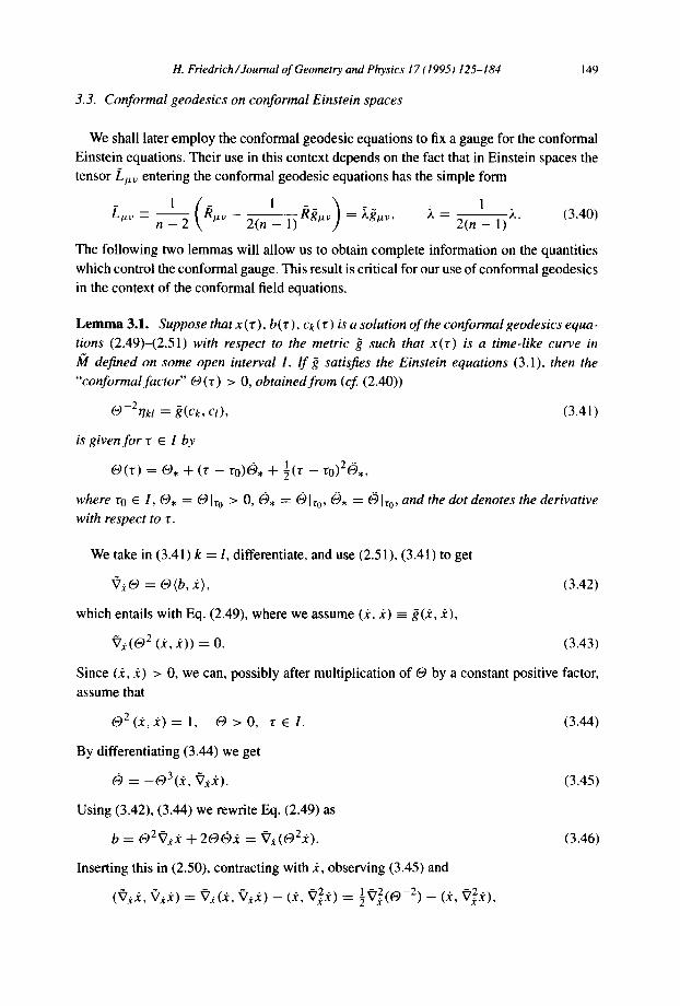
3.3. Conformal geodesics on conformal Einstein spaces
We shall later employ the conformal geodesic equations to fix a gauge for the conformal
Einstein equations. Their use in this context depends on the fact that in Einstein spaces the tensor Lu~ entering the conformal geodesic equations has the simple form
1 ( 1 ) Luv -= - k•v kgtz~ = ~.~'uv, ~. - - - ~. (3.40)
n 2 2 ( n - l ) 2 ( n - l )
The following two lemmas will allow us to obtain complete information on the quantities
which control the conformal gauge. This result is critical for our use of conformal geodesics in the context of the conformal field equations.
Lemma 3.1. Suppose that x ( r ), b( r ) , ck ( r ) is a solution of the conformal geodesics equa-
tions (2.49)-(2.51) with respect to the metric ~ such that x ( r ) is a time-like curve in
1(4 defined on some open interval I. l f ~ satisfies the Einstein equations (3.1), then the
"conformal factor" O ( r ) > 0, obtained from (cf (2.40))
(O-2rlkl : g(Ck, Cl), (3.41)
is given for r ~ I by
O ( r ) = 0), + (r -- r0){~, + l ( ' r -- "r0)2(~,,
where ro ~ I , 69, = Olro > 0, 69, = Olro, ¢0, = ¢0lro, and the dot denotes the derivative with respect to r.
We take in (3.41) k = l, differentiate, and use (2.51), (3.41) to get
V~O = O(b, ~t), (3.42)
which entails with Eq. (2.49), where we assume (~t, ~t) -- ~(~t, ~t),
~'~(O 2 bt, ~t)) = 0. (3.43)
Since (.t, ~t) > 0, we can, possibly after multiplication of 69 by a constant positive factor,
assume that
O 2 (J:, 3C) : 1, O > 0, r E I. (3.44)
By differentiating (3.44) we get
6) = - (93 (k , V.tk). (3.45)
Using (3.42), (3.44) we rewrite Eq. (2.49) as
b = O2~7~t3~ -I- 2 0 0 ~ t = Vot(O23c) . (3.46)
Inserting this in (2.50), contracting with ~, observing (3.45) and
(~7t.l? , V t.I~) : ~(3~, Vx~) -- (.i', ~72.~) = ~Vx( O 1 ~ 2 -2) _ (~, ~72~),
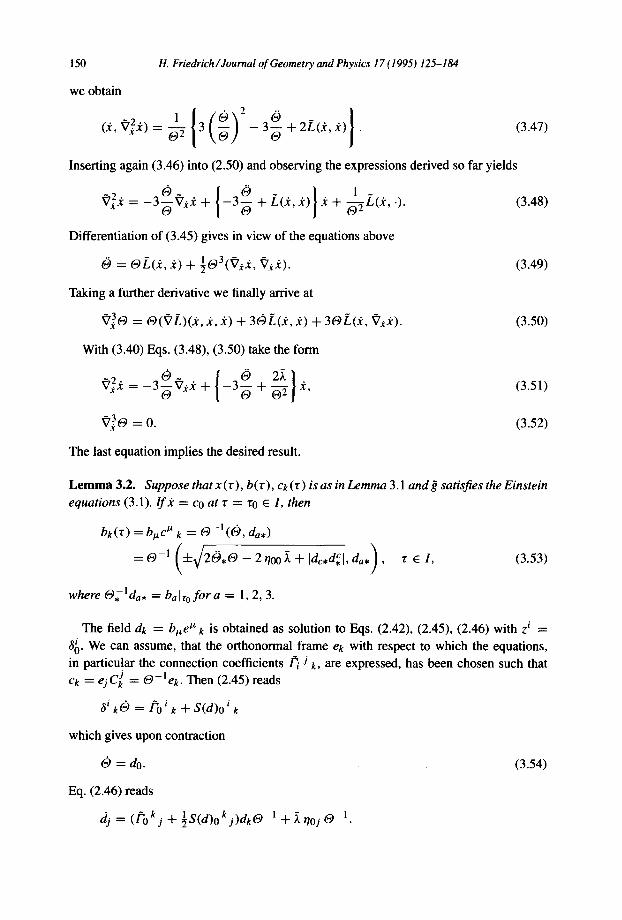
150 H. Friedrich/Journal of Geometry and Physics 17 (1995) 125-184
we obtain
(k, 92~t) = ~ 3 (9 + 2L(~t, £) . (3.47)
Inserting again (3.46) into (2.50) and observing the expressions derived so far yields
} 1 92k = - 3 9~k + - 3 + L(.t, k) ~t + ~--gL(~t, .). (3.48)
Differentiation of (3.45) gives in view of the equations above
= (gL(~t, yc) + ½ 0 3 ( 9 ~ , 9 ~ ) . (3.49)
Taking a further derivative we finally arrive at
9 3 0 = O(VL)(Y¢, Yc, k) + 36)L(~t, .t) + 3oL(:t, 9x~). (3.50)
With (3.40) Eqs. (3.48), (3.50) take the form
(3.51)
(3.52) 9 3 ( 9 = 0 .
The last equation implies the desired result•
Lemma 3.2. Suppose that x (r), b(r), ck (r) is as in Lemma 3.1 and ~ satisfies the Einstein equations (3.1). I f Yc = co at r = ro E I, then
bk(z) =blzclzk = (9-1(6~, da.)
= o - l ( - t - ~ 2 0 , O - 2 000 ~ + ldc,dC.l, d a , ) , t e l , (3.53)
where O f l da. = balrofor a = 1, 2, 3.
The field dk = bueUk is obtained as solution to Eqs. (2.42), (2.45), (2.46) with z i =
8~. We can assume, that the orthonormal frame ek with respect to which the equations, in particular the connection coefficients F / j k, are expressed, has been chosen such that Ck = ejC j = O-lek. Then (2.45) reads
t~i k (9 : ['0 i k "t- S(d)o i k
which gives upon contraction
6) = do. (3.54)
Eq. (2.46) reads
d/= (f'okj + ½S(d)okj)dkO -~ + ~ ooj 0 -~.
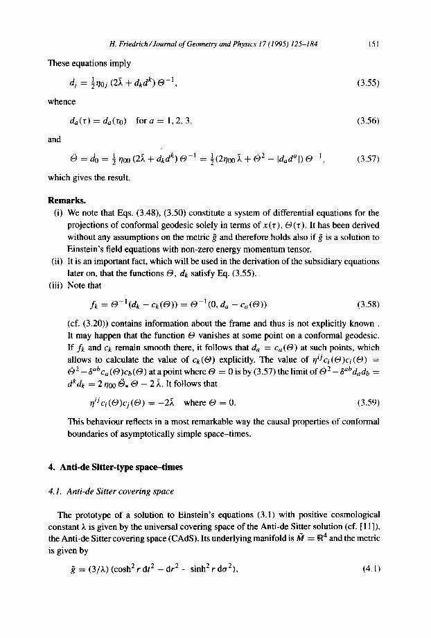
H. Friedrich /Journal of Geometry and Physics 17 (1995) 125-184
These equations imply
dj = ½Ooj (2~. + dkd k) 69-1,
whence
151
(3.55)
da ( r ) -- da (r0) for a = 1, 2, 3, (3.56)
and
D ~ d 0 = I r/oo (2~. + dkdk) 69-1 = ½(2r/00 ~. + (9 2 - I d a d a l ) 6 9 - I , (3.57)
which gives the result.
Remarks. (i) We note that Eqs. (3.48), (3.50) constitute a system of differential equations for the
projections of conformal geodesic solely in terms of x ( r ) , O ( r ) . It has been derived
without any assumptions on the metric ~ and therefore holds also if ~ is a solution to Einstein's field equations with non-zero energy momentum tensor.
(ii) It is an important fact, which will be used in the derivation of the subsidiary equations later on, that the functions 69, dk satisfy Eq. (3.55).
(iii) Note that
fk = 69-1(dk -- ck(69)) = 69-1(0, da - Ca(69 ) ) (3.58)
(cf. (3.20)) contains information about the frame and thus is not explicitly known. It may happen that the function ~9 vanishes at some point on a conformal geodesic.
If fk and ck remain smooth there, it follows that da = Ca(69) at such points, which allows to calculate the value of ck(69) explicitly. The value of oiJci(69)Ci((-~) ) :
(9 2 - 8~bCa (69)Cb(69) at a point where 69 = 0 is by (3.57) the limit of (92 _ ~abdadb :
dkdk = 2 170o 6 . 69 - 2 ~.. It follows that
oiJci(69)cj(69) : -2~. where 69 = 0. (3.59)
This behaviour reflects in a most remarkable way the causal properties of conformal
boundaries of asymptotically simple space-times.
4. Anti-de Sitter-type space-times
4.1. Anti-de Sitter covering space
The prototype of a solution to Einstein's equations (3.1) with positive cosmological constant ~. is given by the universal covering space of the Anti-de Sitter solution (cf. [ 11 ]), the Anti-de Sitter covering space (CADS). Its underlying manifold is M = •4 and the metric
is given by
: (3/~.) (cosh 2 r dt 2 - dr 2 - sinh 2 r dt~2), (4.1)
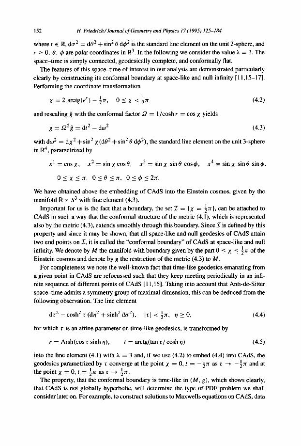
152 H. Friedrich/Journal of Geometry and Physics 17 (1995) 125-184
where t E R, d~r 2 : d0 2 + sin 2 0 d~b 2 is the standard line element on the unit 2-sphere, and
r _> 0, 0, 4~ are polar coordinates in R 3. In the following we consider the value ~. = 3. The
space-t ime is simply connected, geodesically complete, and conformally flat.
The features of this space-t ime of interest in our analysis are demonstrated particularly clearly by constructing its conformal boundary at space-like and null infinity [ 11,15-17].
Performing the coordinate transformation
X = 2 a r c t g ( e r ) - l r e , 0 < X < Ire (4.2)
and rescaling ~ with the conformal factor I-2 = 1/cosh r = cos X yields
g = I22~, = dt 2 - do) 2 (4.3)
with dw 2 = dx 2 + sin 2 X (d02 + s in2 0 d4~2), the standard line element on the unit 3-sphere
in R 4, parametrized by
x I = c o s l , x 2 = s i n x c o s 0 , x 3 = s inx sin0 cos4~, x 4 = s inx sin0 sin4~,
0_<X_<re , 0 < 0 < z r , 0_<c.b_<2re.
We have obtained above the embedding of CAdS into the Einstein cosmos, given by the manifold R × S 3 with line element (4.3).
Important for us is the fact that a boundary, the set 2- = {X = ire}, can be attached to
CAdS in such a way that the conformal structure of the metric (4.1), which is represented also by the metric (4.3), extends smoothly through this boundary. Since 2- is defined by this property and since it may be shown, that all space-like and null geodesics of CAdS attain
two end points on 2-, it is called the "conformal boundary" of CAdS at space-like and null infinity. We denote by M the manifold with boundary given by the part 0 < X < ½re of the Einstein cosmos and denote by g the restriction of the metric (4.3) to M.
For completeness we note the well-known fact that time-like geodesics emanating from
a given point in CAdS are refocussed such that they keep meeting periodically in an infi- nite sequence of different points of CAdS [11,15]. Taking into account that Anti-de-Sitter
space-t ime admits a symmetry group of maximal dimension, this can be deduced from the following observation. The line element
d r Z - c o s h 2 r ( d r / 2 + s i n h Z d c r 2 ) , Irl < ½re, I / > 0 , (4.4)
for which r is an affine parameter on time-like geodesics, is transformed by
r = Arsh(cos r sinh r/), t = arctg(tan r / c o s h r/) (4.5)
into the line element (4.1) with ~. = 3 and, if we use (4.2) to embed (4.4) into CADS, the geodesics parametrized by r converge at the point X = 0, t = -½re as r ~ -½re and at the po in tx = 0 , t = ½ r e a s r ~ I jr.
The property, that the conformal boundary is time-like in (M, g), which shows clearly, that CAdS is not globally hyperbolic, will determine the type of PDE problem we shall consider later on. For example, to construct solutions to Maxwells equations on CADS, data
H. Friedrich/Journal of Geometry and Physics 17 (1995) 125-184 153
have to be prescribed on a space-like hypersurface which extends like {t = 0} up to 2- and
on the boundary 2- at space-like and null infinity.
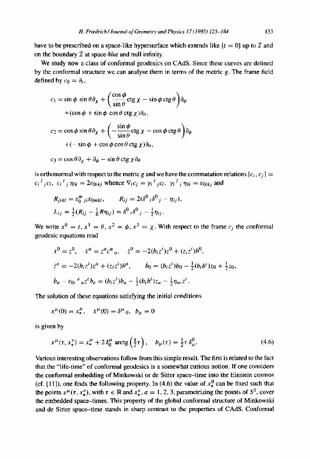
We study now a class of conformal geodesics on CADS. Since these curves are defined by the conformal structure we can analyse them in terms of the metric g. The frame field
defined by co = Or,
/cos~ . ) cl = s i n s s in00 x + ~ si-~-0-ctgx - s i n < p c t g 0 0~
+(cos q~ + sin q~ cos 0 ctg X)00,
f s i n q ~ ) c2 = cos tp sin 00 x + ~. - s i - ~ c t g x - cosq~ctg0 0~
+ ( - sin q~ + cos ~p cos 0 ctg X)Oo,
c3 = cos 0O x + 0~ - sin 0 ctg X O0
is orthonormal with respect to the metric g and we have the commutation relations [ci, cj ] =
ci I j c l , ci I j rllk = 2eOikj whence V i C j -~- Yi I j c l , Yi l j rllk = 80ikj and
Rjikl ~-" m =-. _ E 0 jiEOmkl, R i j 2(8 ° i~Oj rlij),
L,j = ½(Rij - R ij)= go i oj _ ½o,j.
We write x ° ---- t, x I ---- 0, x 2 = tp, x 3 ---- X- With respect to the frame cj the conformal
geodesic equations read
~o = z O, Jcc~ = zac a a, ~0 = _ 2 ( b i z i ) z 0 -I- ( z i z i ) b O,
~a : _ 2 ( b i z i ) z a d- ( z i z i ) b a, [~0 : (b i z i )bo - l ( b i b i ) z o -b l z o ,
ba - e o c e a z C b e = (b i z i )ba - l (b ib i ) za 1 z c - ~ O a c •
The solution of these equations satisfying the initial conditions
x t Z ( 0 ) = x . ~, ~ t ~ ( 0 ) = 8 ~0, b~ = 0
is given by
( 1 ) o xlZ(r ,x , v ) = x ~ + 2 8 ~ arctg r , b ~ ( r ) = ½ r S ~ . (4.6)
Various interesting observations follow from this simple result. The first is related to the fact that the "life-time" of conformal geodesics is a somewhat curious notion. If one considers the conformal embedding of Minkowski or de Sitter space-t ime into the Einstein cosmos (cf. [11]), one finds the following property. In (4.6) the value of x ° can be fixed such that the points x~ (r, x.),v with r ~ R a n d x a , a = 1, 2, 3, parametrizing the points ofS3, cover
the embedded space-times. This property of the global conformal structure of Minkowski and de Sitter space-t ime stands in sharp contrast to the properties of CADS. Conformal
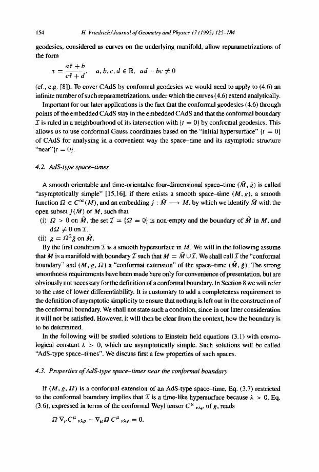
154 H. Friedrich/Journal of Geometry and Physics 17 (1995) 125-184
geodesics, considered as curves on the underlying manifold, allow reparametrizations of the form
af +b r - c f + ~ , a,b,c, d E R , a d - b c ¢ O
(eft, e.g. [8]). To cover CAdS by conformal geodesics we would need to apply to (4.6) an infinite number of such reparametrizations, under which the curves (4.6) extend analytically.
Important for our later applications is the fact that the conformal geodesics (4.6) through
points of the embedded CAdS stay in the embedded CAdS and that the conformal boundary
I is ruled in a neighbourhood of its intersection with {t = 0} by conformal geodesics. This
allows us to use conformal Gauss coordinates based on the "initial hypersurface" {t = 0} of CAdS for analysing in a convenient way the space-time and its asymptotic structure
"near"{t = 0}.
4.2. AdS-type space-times
A smooth orientable and time-orientable four-dimensional space-time (AIr, ~) is called
"asymptotically simple" [15,16], if there exists a smooth space-time (M, g), a smooth function Y2 E C °° (M), and an embedding j : Aqr > M, by which we identify/~t with the open subset j (/~/) of M, such that
(i) ~2 > 0 on M, the set 2- = {12 = 0} is non-empty and the boundary o f / ~ in M, and
d/2 # 0 on 2-. (ii) g = ff22g on M.
By the first condition 2- is a smooth hypersurface in M. We will in the following assume
that M is a manifold with boundary 2 such that M = M 132-. We shall call I the "conformal boundary" and (M, g, I2) a "conformal extension" of the space-time (AT/, ~). The strong
smoothness requirements have been made here only for convenience of presentation, but are
obviously not necessary for the definition ofa conformal boundary. In Section 8 we will refer to the case of lower differentiability. It is customary to add a completeness requirement to
the definition of asymptotic simplicity to ensure that nothing is left out in the construction of the conformal boundary. We shall not state such a condition, since in our later consideration
it will not be satisfied. However, it will then be clear from the context, how the boundary is to be determined.
In the following will be studied solutions to Einstein field equations (3.1) with cosmo- logical constant X > 0, which are asymptotically simple. Such solutions will be called "AdS-type space-times". We discuss first a few properties of such spaces.
4.3. Properties of AdS-type space-times near the conformal boundary
If (M, g, $2) is a conformal extension of an AdS-type space-time, Eq. (3.7) restricted to the conformal boundary implies that 2" is a time-like hypersurface because ~. > 0. Eq. (3.6), expressed in terms of the conformal Weyl tensor C tz vxp of g, reads
~2 V~C ~ ~xp - VuY2 C ~ ~xp = O.
s : t 3 x / ~ ,
Da dac = O,
where
H. Friedrich/Journal of Geometry and Physics 17 (1995) 125-184 155
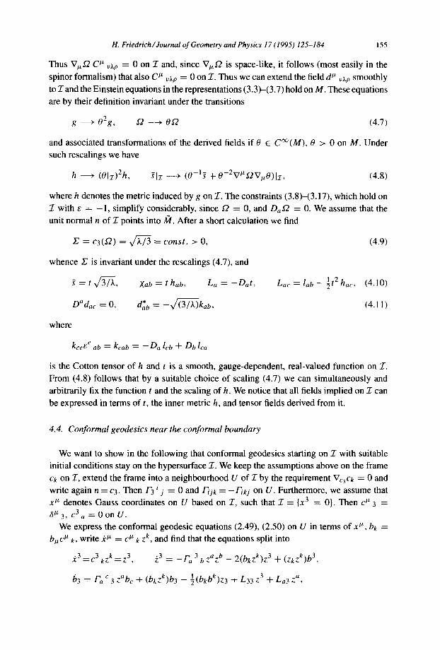
Thus VuS2 C u vzp = 0 on 2- and, since Vul-2 is space-like, it follows (most easily in the
spinor formalism) that also C u v~p = 0 on 2-. Thus we can extend the field d Iz vxp smoothly
to 2- and the Einstein equations in the representations (3.3)-(3.7) hold on M. These equations are by their definition invariant under the transitions
g > 02g, ~ ~ 012 (4.7)
and associated transformations of the derived fields if 0 E C ~ ( M ) , 0 > 0 on M. Under
such rescalings we have
h > (01~:) 2h, glz > ( 0 - I s -t- 0-2V~I2Vtz0) lz , (4.8)
where h denotes the metric induced by g on 2-. The constraints (3.8)-(3.17), which hold on
2- with e = - 1 , simplify considerably, since 12 = O, and Da,(2 : O. We assume that the
unit normal n of 2- points into/~/. After a short calculation we find
~' = C3(A'2 ) = ~/-~/3 = cons t . > O, (4.9)
whence 2? is invariant under the rescalings (4.7), and
Xab = t hab, La = - D a t , Lac = lab - l t2 hac, (4.10)
d* b : - - v /~ /~ . ) kab , (4. I I)
kce 6e ab = kcab = - O a lcb q- Db lca
is the Cotton tensor of h and t is a smooth, gauge-dependent, real-valued function on 2-.
From (4.8) follows that by a suitable choice of scaling (4.7) we can simultaneously and
arbitrarily fix the function t and the scaling of h. We notice that all fields implied on 2- can
be expressed in terms of t, the inner metric h, and tensor fields derived from it.
4.4. Conformal geodesics near the conformal boundary
We want to show in the following that conformal geodesics starting on 2- with suitable
initial conditions stay on the hypersurface 2-. We keep the assumptions above on the frame
ck on 2", extend the frame into a neighbourhood U of 2- by the requirement Vc3ck = 0 and
write again n =c3 . Then if3 i j = 0 and ffijk = --f f ikj on U. Furthermore, we assume that
x " denotes Gauss coordinates on U based on 2-, such that 2- = {x 3 = 0}. Then c ~ 3 = •#3, C3a = Oon U.
We express the conformal geodesic equations (2.49), (2.50) on U in terms of x tz, bk =
b~c Iz k, write .ic ~ = c Jz k Z k, and find that the equations split into
3~3 = C 3 kZ k = Z 3, ~3 = --]-'a 3 b zaz b -- 2(bkzk)z 3 + (ZkZk)b 3,
b3 -~ Fa c3 zabc + (bkzk)b3 - l (bkbk)z3 + L33 z 3 + La3 z a,
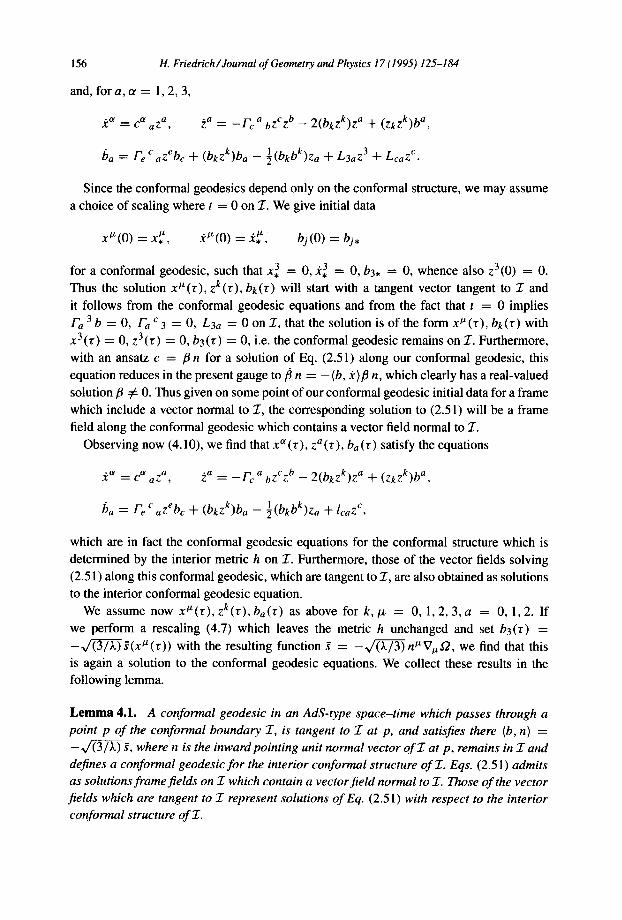
156 H. Friedrich/Journal of Geometry and Physics 17 (1995) 125-184
and, for a, u = 1,2, 3,
~a = C a aZ a, ~a = _ F c a b z C z b 2 ( b k z k ) z a + ( z k z k ) b a,
ba = fie c azebc + (bkzk)ba _ l (bkbk)z a + L3aZ 3 + LcaZ c.
Since the conformal geodesics depend only on the conformal structure, we may assume
a choice of scaling where t = 0 on 2". We give initial data
x~'(o) = x , ~, . e ' ( o ) = ~,~, h i (o) = b j ,
for a conformal geodesic, such that x 3 = 0, ~3 = 0, b3. = 0, whence also z3(0) = 0.
Thus the solution xV(r), zk(r), bk(r) will start with a tangent vector tangent to 77 and
it follows from the conformal geodesic equations and from the fact that t = 0 implies
Fa 3 b = O, Fa c 3 = O, L3a = 0 on 77, that the solution is of the form xV(z), bk(r) with
x3(r ) = 0, z3(r) = 0, b3(r) = 0, i.e. the conformal geodesic remains on 2-. Furthermore,
with an ansatz c = /~ n for a solution of Eq. (2.51) along our conformal geodesic, this
equation reduces in the present gauge to/~ n = - ( b , .,?)/5 n, which clearly has a real-valued
solution/5 # 0. Thus given on some point of our conformal geodesic initial data for a frame
which include a vector normal to 77, the corresponding solution to (2.51) will be a frame
field along the conformal geodesic which contains a vector field normal to 2".
Observing now (4.10), we find that x a (r) , z a (r) , ba (r) satisfy the equations
~a = C a aZ a, ~a = _ f fc a b z C z b 2 ( b k z k ) z a + ( z k z k ) b a,
[~a : Fe c azebc + (bkzk)ba _ l (bkbk)z a + lcaz c,
which are in fact the conformal geodesic equations for the conformal structure which is
determined by the interior metric h on 77. Furthermore, those of the vector fields solving
(2.5 l) along this conformal geodesic, which are tangent to 77, are also obtained as solutions to the interior conformal geodesic equation.
We assume now x~( r ) , zk(r), ha(r) as above for k, /z = 0, 1, 2, 3, a = 0, l, 2. If
we perform a rescaling (4.7) which leaves the metric h unchanged and set b3(r) =
- ~ ' ( 3 / i ) g(xV(r)) with the resulting function g = -~ /~-7-~nVVt , /2 , we find that this is again a solution to the conformal geodesic equations. We collect these results in the following lemma.
Lemma 4.1. A conformal geodesic in an AdS-type space-time which passes through a
point p o f the conformal boundary Z, is tangent to Z at p, and satisfies there (b, n) =
- ~ f~ / k ) g, where n is the inward pointing unit normal vector o f Z at p, remains in Z and
defines a conformal geodesic for the interior conformal structure o f 2-. Eqs. (2.5 1) admits
as solutions frame fields on 2- which contain a vector field normal to Z. Those o f the vector
fields which are tangent to Z represent solutions o f Eq. (2.5 1) with respect to the interior conformal structure o f Z.
H. Friedrich/Journal of Geometry and Physics 17 (1995) 125-184
5. Formulation of the initial boundary value problem
157
5.1. General considerations, gauge conditions and initial data
Suppose that (M, g, $2) is a conformal extension of an oriented and time-oriented CADS-
type space-time (AT/, ~) which does not contain any closed causal curve, but which contains
a smooth, oriented, compact, space-like hypersurface S with boundary OS which intersects
the conformal boundary Z such that S N Z = OS. We assume that the causal future J+(S)
of S coincides with the future domain of dependence of the set S U Z + and that this set can
be mapped diffeomorphically onto [0, l [ x S such that Z + is mapped onto [0, l [ × OS. We
denote here by/7+ the part of 2- in the future of S (including OS). For the causal notions
used here and in the following we refer to [l 1]. The rest of this article is devoted to the
initial boundary value problem which we need investigate to answer the question:
Which data implied by ~ respectively g, S2 on S U 17 + do we need, to reconstruct in
a neighbourhood of S in J+(S) up to diffeomorphisms the solution ~ of Einstein's field
equations (3.1) with positive cosmological constant ;~ ?
It is well known (cf. [4]) that h, ~, the first respectively second fundamental form induced
on S = S \ 0S by ~, are the data which determine the solution ~ of (3.1) uniquely on the
domain of dependence of S up to diffeomorphisms. These fields satisfy the constraint
equations
b ' % ~ - b t ~ '~ ,, = 0, ? _ (~,~ ,,)2 + ~ , ~ = 2 ~ (5. l)
induced by (3.1) on S, where b denotes the Levi-Civita connection and ~ the Ricci scalar
of h. On S we may choose I2 = Y2, and ~7 = h(.f2) = ~ , , where h denotes the future
directed unit normal field of S with respect to ~. The functions 12,, Z', are restricted only by
smoothness and positivity requirements and by their behaviour near OS, where we require
in particular Z' = n(~2) = Y2,1Z, to be smooth. Here n denotes the future directed unit
normal field of S with respect to g. We can now determine the first respectively second
fundamental form
h~/~ = 1-22h~, X~/~ = $2()~c~¢~ + z'/Ttc~/~) (5.2)
of g on S and, as will be shown later on, all initial data on S for the conformal field equations.
To answer the question, which data may be prescribed on the boundary, we cannot fall
back on known results and it should be discussed in conjunction with the evolution equations.
To determine the form of these equations we have to decide in particular on a specific gauge,
i.e. on a choice of the conformal scaling, of the orthonormal frame, and of a coordinate system near the "initial hypersurface" 2-. We shall describe now how to fix a gauge in terms of the conformal geodesic equations. To simplify the discussion, it is convenient to assume
that the intial hypersurface S has been chosen such that the unit normal vector field n is
tangent to 2- on 0S, i.e.
Z' = n(S2) = 0 on OS. (5.3)
158 H. Friedrich/Journal of Geometry and Physics 17 (1995) 125-184
This allows us to choose
, U = 0 o n S . (5.4)
Observing (4.8) the function I2, is chosen such that
.~ = 0 on 0S. (5.5)
We assume that at each point of S starts a future directed conformal geodesic x~( r ) , by (r),
ck(r) with r = 0 on S, such that we have on S in terms of the metric ~ and its associated
Levi-Civita connection
future directed, orthogonal to S, ~(~t, ~) = ~Q-2,
b = .(-2 - I dl2 whence (b, ~) = 0,
CO = JC, g(ci , Cj) ----- ~ - 2 rlij '
(5.6)
(5.7)
(5.8)
where the second equation in (5.7) follows from (5.4). We note here that once the gauge
has been fixed by (5.6), (5.7), neither the point set run through by a conformal geodesic nor
its parameter r depends on the remaining freedom of prescribing on S the frame satisfying
(5.8). The following statements will be true in a suitably determined neighbourhood W of S in
J + (S) which is chosen such that its intersection with each conformal geodesic is connected.
The curves xU(r) define a smooth, time-like congruence in W, ck a smooth frame field, and
bvdx ~ a smooth l-form. If we set x ° = r on W and extend a local coordinate system xct,
a = 1, 2, 3, on S into W by the requirement that x ~ remains constant along the conformal
geodesics, we obtain smooth local coordinates x u , / z = 0, 1, 2, 3, on W, which we shall
call conformal Gauss coordinates based on S. The coefficients c u k = (dx u, c~) of Ck with
respect to the conformal Gauss coordinates satisfy on W c u 0 = 8 u 0, but in general c o a = 0
only on S. We fix a smooth conformal factor 12 whence the metric g on W by requiring
g(ci, Ck) = rlik. In terms of the metric g and its Levi-Civita connection V the conformal geodesics are represented by (3.20) in the form x~(r ) , fv ( r ) , Ck(r) with
f u = b~ - ~ - ! V~ I2, (5.9)
such that f u = 0 on S. It follows from Lemma 4.1, the assumption (5.5), and the initial conditions that the conformal geodesics starting on 0S remain in 2 -+. Because of (5.5) we can write g = I2, s, with a smooth function s, on S. From the initial conditions, Lemmas 3.1, 3.2, and (3.17) follows on W
I2 = ~ , (1 - ½r2s , ) , (5.10)
and
bk = ~2-1(~2, da,) with da, = ( c ~ O c t S 2 ) , , (5.11)
where we assume, that the functions I2,, s, , (cct a Oct ,.(2 ) , , initially defined on S, are extended to W such that they are constant along the conformal geodesics.
H. Friedrich/Journal of Geometry and Physics 17 (1995) 125-184 159
We will adopt in the following the notation used in our discussion of the conformal
Einstein equations in Section 3. The conformal field equations will be expressed with
respect to the connection V given by
- V = S(b), respectively x~ - V = S ( f ) .
On S the connection V coincides with the connection V defined by g. Thus we have on S
for the connection coefficients with respect to the frame ck
ffaCb = l"aCb, - - f faOc hcb = f fabo = Xa b = XaflCC~aCflchCb ,
Fa °o = O, (5.12)
with
Fad b Ca = OcaCb, Xab = g(£7c~C0, Cb),
where D denotes the Levi-Civita connection defined by the metric h induced by g on S. By
our choice of gauge we have
rOik =0, ffOj = 0 on W. (5.13)
Using (5.9) and the connection defined by g to express (2.35) on S, we find
ffaj = (d30, Ca) - t j a = - t j a ,
where Ljk = Alzvc# j C v k and
A u v = _ i f 2 - 1 V i x V v f f 2 .q_ I guy ~ - 2 V a I 2 Va$2 + 112-2;~guv
since g is conformal to a solution to Ric[~] = ~.~. Using the data given so far and (5.4),
(3.8), (3.16), (3.17) we find
ffaO = ~('2-1 Xa b Dba,2, + cd, h f ' a b = g - 2 - 1 { D a D b ~ 2 - - 1 D c D C f f 2 h a b } - - l { r - - ( X c C ) 2 XcdX l a b (5.14)
Using (3.15), (3.16) the rescaled Weyl tensor d i jkl can be determined. It is specified com-
pletely by
dab =-- daObO = $ 2 - 2 { Oa D b ff2 - l h a b O C Oc I2 + ~'2 (lab -- l r hab ) ]
-] -at2-1 [XCc Xab -- XCa Xcb -- l ha b ((XCc)2 _ xCd Xcd)} (5.15)
and
dabc =~ daObc = ,(2-1 { D b Xca - Dc Xba -- ha[b De Xcle -I- ha[b Dcl X e e } ,
or equivalently,
d* b = -I-2 - I De Xf(a Eb) ef (5.16)
| 60 H. Friedrich/Journal of Geometry and Physics 17 (1995) 125-184
It Can be shown (cf. [6]), that the conformal data so defined satisfy in fact the constraints
(3.8)-(3.17) on S.
Definition. Initial data/~t~, )2,~ solving on the manifold S the constraint equations implied by (3. l) are said to satisfy the condition of "asymptotic simplicity", if the conformal data
derived from them as above extend smoothly to OS.
This definition raises the question of "how many" such data exist. This problem will not
be discussed in detail in this article. However, to illustrate the nature of the problem, we remark on an important subclass of data for which the complete analysis has been given.
In analogy to the condition of time-symmmetry in the standard Cauchy problem for Einstein's field equations we consider the case
)(ab = 0 on S. (5.17)
It follows then from (5.4) that also Xab = 0 on S. As described above, we can then determine
all conformal data on S from hab. We find from (3.9), (3.15), (3.16), (3.8) that La = O,
dabc = O, l r = I a = L a - $ ' 2 1 r + on a a, I D a D a ~ = ~ S and thus can write (3.17) in the form
2 I2 DaDa$2 ---- - l r $'22 d- )~ q- 3 Da~-2Da$2. (5.18)
Setting in this equation I2 = 1, or rewriting it in terms of the metric h = $2-2h induced by on S \ 0 S, we see that (5.18) is equivalent to the Hamiltonian constraint ? = 2~. = const. > 0 which we assumed to be satisfied by hab.
The construction of solutions to this constraint, which satisfy the fall-off conditions which
are implicit in the smoothness requirement on the conformal fields, has been described in all details in [2] where the following result has been shown (observe the different signature used in that article, the metric h used here is negative definite).
Suppose ~. is a positive real number, S is a smooth, compact, orientable, three-dimensional manifold with boundary OS, and h is a smooth, negative definite metric field on S. Denote
by tz the second fundamental form induced by h on 8S and by #* its trace free part with respect to the first fundamental form on OS. If and only if the metric h is such that the conformally invariant condition
/z* = 0 on OS (5.19)
is satisfied, there exists a (unique) solution g2 ~ C°°(S) of (5.18) with .f2 > 0 on S \ OS,
I'2 = 0, dI2 ~ 0 on OS and it follows that the fields given on S \ OS by
E = 0 , g = ½OaOa~-2 + ~--~$'2r, La = 0 , dabc = 0 ,
Lab -~- --g2-1(Oa Ob~2 -- 1 Oc OC~,-2hab) + 1 rhab,
dab = ~-2-2{Do Db~'2 -- 1 Dc DC$-2 + $2(lab -- l r hab)}
extend smoothly to S and solve there the constraint equations (3.8)-(3.17).
H. Friedrich/Journal of Geometry and Physics 17 (1995) 125-184 161
It turns out that if the condition (5.19) is not satisfied, there still exists a unique solution
I2 of (5.18) which is positive on S \ 0 S and vanishes on 0 S. This solution will be smooth on
S also under conditions slightly weaker than (5.19). In any case, if (5.19) is not satisfied, the field dab(P) diverges like p ( p ) - 2 as the distance p(p) of the point p ~ S from the part of the boundary OS where (5.19) is violated goes to zero. Most likely this blow-up behaviour
will spread and the solution of the conformal field equations determined by the data on S \ OS will blow up at parts of the boundary of its domain of existence. If such a spreading
of the blow-up behaviour does occur, it should "most easily" be established by using the conformal field equations, which would allow to localize the problem to a neighbourhood
of OS. Since the conformal factor will be bounded below by a positive number near most
parts of the boundary of the domain of existence, also the "physical" conformal Weyl tensor will diverge at parts of the boundary. Thus we would obtain a statement on the blow-up
behaviour of the physical fields not depending on the use of the conformal method. This
suggests that smooth AdS-type space-times with boundary at space-like and null infinity which is diffeomorphic to R x OS exist only if the initial data implied by the "physical"
metric ~, satisfy the fall-off conditions encoded in the smoothness requirement of asymptotic simplicity.
Recently, in a context somewhat different from the one discussed here, the investigations in [2] have been generalized into various directions, in particular to the case where the
second fundamental form ~(ab does not vanish [1 ]. By the methods developed in [1] the
existence of a more general class of data satisfying the condition of asymptotic simplicity can be shown.
5.2. The reduced field equations
In the following ck will always denote the specific frame field on hT/determined by the gauge discussed in Section 5.1 and a k the dual 1-form field. We shall employ a splitting
of fields with respect to the time-like vector field ~v'~c0, which in the frame coa, has the representation
~.aa' = EO aEO ' a' q_ 81 abl ' at (5.20)
With the exception of the factor ~ in (5.21) we will follow the conventions of [7]. For later use we need, however, more details about the underlying structures. The coefficients
(5.20) are used to define the projected van der Waerden symbols
~Tj ab =¢3rj (aa I~'b)at, ¢YJab = ~(ba'crJa)a I,
such that ao ab aO ab both vanish and
b ' ' " ' b ~J k = ~ J a b ( T k ab, j = 1 , 2 , 3 , Eab Ea , = I raa, rbb -~-~JafZ' fa , '~eb ~je ,
rljk aJ ab O'k cd = -- ~jk ~7J ab ~Tk cd = --Ea(ced)b ~ habcd.
The simply connected group which leaves eab as well as Tab' invariant is given by
SU(2, C) = {t a b E SL(2, C) I raa ' tabU' b' = rbb'}.
162 H. Friedrich/Journal of Geometry and Physics 17 (1995) 125-184
There is a surjective 2 : 1 group homomorphism
ca" • " t a cd S U ( 2 , C) g tao---> t ' j : a t a b ctbdcYj E O+ (3, R),
where i, j = 1, 2, 3. It implies an isomorphism of Lie algebras which is given by
su (2 , C) 9 u a b ~-~ u i j : 2 f f i a b U a c c r j c b E o(3, •)
and has inverse
o(3, R) 9 b l i j U a b ~--- l u t j f f i a c ~ J b c E su(2 , C) .
For any frame eaa, = eka k aa' with e0 = co we get a decomposition
= 1_ bb p eaa' -~ taa ,T ebb, _ ~b area b
• b ~ a I with r b ebb, = ~/~co and a frame eab ~- r(b ea)a r in the subspace orthogonal to co which
satisfies, with respect to the metric h induced by g on that subspace, the normalization
condition h(eab, ecd) = habcd.
At p e M the vector co induces a hermitian form which for spinors x , /z is defined
by (x, # ) ~ ~/2g(co , x/2). The set of spin frames 8 e SL(19I) which are normalized with respect to this hermitian form by qC2g(co, ~a ~a') = Z'aa' defines a subbundle SU(I(/1)
of SL(I(/I) with structure group S U ( 2 , C). The structure of this group is reflected by the
property of the spin frames 6 E S U ( ~ I ) that the normalized spinor 80 determines uniquely
the spinor 81 and vice versa• The map which associates with 8 E SU(191) the frame e~bak ab is a 2 : 1 bundle morphism
of SU(1(4) onto the bundle of positively oriented frames orthogonal to co with respect to the homomorphism q~".
Any spinor field on M supplies an invariant function on SU(i f4) and vice versa• If/Za, is the function corresponding to a primed spinor field, we define a bijective complex linear map
a t
IZa ' -">" ]J~a : 'ra ~a ' which allows to associate with any primed spinor field an unprimed
spinor field. This map is extended in an obvious way to spinor fields of higher valence and various index positions such that it commutes with contractions. It should be observed
that the position of the contracted index of r aa' is always chosen as shown above. The map is related to the hermitian conjugation map which associates to any unprimed spinor
a I _
field another such field by #~ --+ # + = ra /Za'. Again, this map is extended by complex semi-linearity to more general spinor fields such that it commutes with contractions and satisfies, e.g. lz ++ = (--1)kl2al...ak. al ...ak
If a tensor field/~ is represented at 8 6 S U ( t f l ) by the components gala, 1 ...aka k ,, it can be £ / t -
expanded in terms of the components of the frame eab = ~(a rb) S a, orthogonal to co if • aja!
and only if it is "spatial", i.e. ff r J IZala~l ...aja,j...aka~k = 0 for j = 1 . . . . . k. In that case the
components of /z in the frame eab are given by
t alklZ . . . . U(albl) . . . (akbk)" ll~albl...akbk -~- 7;bl al • • • ~bk alal . . .ajaj . . .aka k
H. Friedrich/Journal o f Geometry and Physics 17 (1995) 125-184 163
Conversely, any spinor field with 2k unprimed indices which has the symmetries in the
index pairs considered above corresponds to a spatial spinor. For a tensor field # which
is represented on S U ( 1 ( 4 ) by a component function/za~, this tells us, that we obtain an orthogonal splitting by writing IZaa, = "Cca, rcb'IZab, 1 , cc' , _ T:c = raa r Ltcc a ' # c a , where Iz, a =
b' r~c IZa)b' represents the spatial part of/~. Again, this procedure can be extended in an obvious way to spinors of higher valence.
Finally we note that a spatial tensor which is represented by the component function
lZalbl ...akbk = lZ(atbt )...(akbk) represents a real tensor field if and only if it satisfies the reality
condition #+ = ( - 1)k#a I bl ...akb k . albl ...akbk We shall discuss now the data and the propagation equations inherent in the conformal
Einstein equations in terms of spinors and the gauge discussed in Section 5.1. By x u will
be denoted conformal Gauss coordinates and we will sometimes write as before r -- x °. The frame vectors are projected onto
!
T a d ~ Or, = Cl z abOla. Caa' = Cab = ~'(a a Cb)a '
We set
b ~ b ~ Fabcd = rb Fab'cd, l a b = rb )Cab,,
b ~ c' d ~ - a ~ c' ~v/2 Xabcd ~ - -F 'abdc- l - ~b 75 c T d l-'ab,c,d, = "gb (Vaa , Tcc,)~d , (5.21)
a' b' t~acbd = T c 75d ¢IJaa,bb ~ .
From the gauge conditions (5.1 3) follow t
A b = f b ~ , F c C o b = r cc F c c ' o b = - A b ,
x / ~ X(ab)cd ----- ~ / 2 Xabcd - - g-ab f c d , ¢i)c c bd = O.
The initial data on S are given in terms of spinor expressions as follows: (i) The coefficients c a ab are determined by the choice of the frame ck. This choice is not
critical away from the boundary OS. T h e specific choice near the boundary will be discussed later on. By our gauge conditions c o ab = O.
(ii) Again, by our gauge f a b = O.
(iii) Let Dab denote the covariant derivative in the direction of Cab with respect to the con-
nection D and define connection coefficients Yabcdef by setting Da b Ce f = Yab cd e fCcd.
The coefficients Yabcd = _ 21 Yabcf d f satisfy Yabcd = Y(ab)(cd). The second fundamen- tal form on S is given by Xabcd ~ g(VcaoCO, Ccd) and coincides because of our gauge conditions with the restriction of (5.21) to S. It satisfies Xabcd = X(ab)(cd) = Xcdab.
The connection coefficients Fabcd are given by
1 Fabcd = Yabcd -- - ~ X a b c d .
Defining for the function Yabcd the operation of hermitian conjugation by the same formal rule as for invariant functions, we find that the two terms in the last expression
may be distinguished by using the properties
+ + }/abcd : --) tabcd' Xabcd : )(abcd.
164 H. Friedrich/Journal of Geometry and Physics 17 (1995) 125-184
(iv) It follows directly from (5.13), (5.14) that
¢l)abc d = $2-1DabDcd$2 -- l $2-2habcd{3 Def $2 D ef $2 + ~.}
--Ecd -~2 ~r2 - 1Xab ef Def $2
= $2-1D(ab Dcd) $2 -- ~2{r - (Xef ef)2 Jr- XefghX efgh } h~bcd --Scd -~2 $2-1Xab ef Def $2.
(v) Denoting by Sabcd the trace-free part of the Ricci tensor of h, we finally get
CPabcd = dabcd + id*bcd = $2-2 D<~bDcd)$2
+$2-1 (Sabcd -t- X ef ef X(abcd) -- X ef (abXcd)ef d- V/-2D f (aXbcd)f)"
It may be noticed that the first four terms on the right-hand side of the last equation represent real spatial tensors while the last term represents a purely imaginary spatial tensor on S. This corresponds to the decomposition into the electric part dabcd and the magnetic part d*bc d which both represent real spatial tensors.
The propagation equation will be expressed with respect to the covariant directional derivative operators
a t P = raa'Vaa ', ~)ab : r(a Vb)a',
given explicitly by
P = V00, + VII, = v~Or, ~)01 = l ( v 0 0 ' - - V l l ' ) ,
D 0 0 = - - V 0 1 , , D I I = V I 0 ' .
We want to extract from Eqs. (3.35) to (3.39) a system of propagation equations for the unknowns
C# ab, ffabcd, t~acbd, ~acbd. (5.22)
These equations will imply in particular equations for
fab, Xabcd,
which for later convenience will be added to the list. For Eqs. (3.35)-(3.38) the choice of evolution equations is suggested by our gauge conditions. Contracting these equations with r cc' and projecting as indicated above, we get with $2 as in (5.10) and with
dab = (cct abOc~$2 ) . , ( 5 . 2 3 )
derived from (5.11),
Or ¢0 ab = -- fab -- X(ab) ef cO ef , (5.24)
Or Ca ab ~--- --X(ab) ef cct ef , Ot : 1, 2, 3, (5.25)
1 f Or fab = -- Z(ab) ef f e f -- -'~ (1)abf , (5.26)
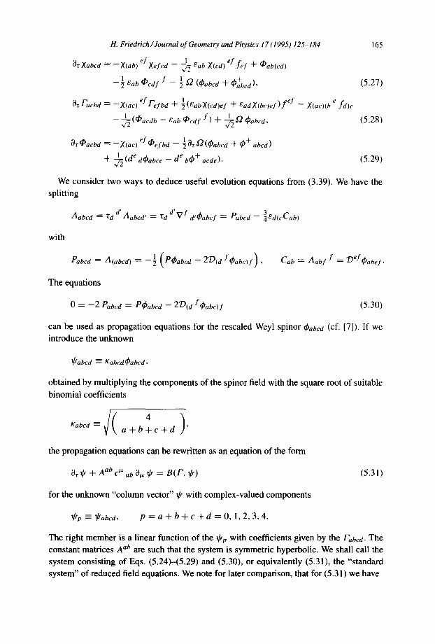
H. Friedrich /Journal of Geometry and Physics 17 (1995) 125-184 165
OrXabcd ~ --X(ab) ef xefcd -- ~2 6ab X(cd) ef f e f + ¢l)ab(cd)
1 _ f + 2 Cab (Pcdf _ 1 ~f2 (~abcd q- ~)abcd ), (5.27)
1 e Or~cbd = --X(ac)ef Fefbd + ~(8abX(cd)ef + eadX(bc)ef ) f ef -- X(ac)(b fd)e
f) q~ (¢l)acdb -- Cab ¢I)cdf -'[- ~ ~ ~abcd, (5.28)
Or ¢l) acbd ~- -- X (ac) ef ¢l) e f O d _ ½0z ~'2 ( ~abcd -~- (P + abcd)
+ -~2 (de debaOce -- d e 04) + acde). (5.29)
We consider two ways to deduce useful evolution equations from (3.39). We have the splitting
d t r Aabcd = ~'d Aabcd' = Td d v f d'~abcf Pabcd -- 3 = ~8d(cCab )
with
eabcd = A(abcd) = _ 1 (e~abcd -- 2"~(df~babc) f ) , Cab "~- Aabf f = "~ef~abef.
The equations
0 = - 2 Pabcd = P~Pabcd -- 2D(d fqbabc)f (5.30)
can be used as propagation equations for the rescaled Weyl spinor ¢babcd (cf. [7]). If we introduce the unknown
lJtabcd ~ Kabcddt)abcd,
obtained by multiplying the components of the spinor field with the square root of suitable binomial coefficients
a + b + c + d '
the propagation equations can be rewritten as an equation of the form
Or~ + A ab c u ab O# ~ • B ( F , ~ ) (5.31)
for the unknown "column vector" ~p with complex-valued components
~ p ~ a b c d , p = a + b + c + d = O , l , 2 , 3 , 4 .
The right member is a linear function of the ~p with coefficients given by the Fabcd. The
constant matrices A ab are such that the system is symmetric hyperbolic. We shall call the system consisting of Eqs. (5.24)-(5.29) and (5.30), or equivalently (5.31), the "standard system" of reduced field equations. We note for later comparison, that for (5.31) we have
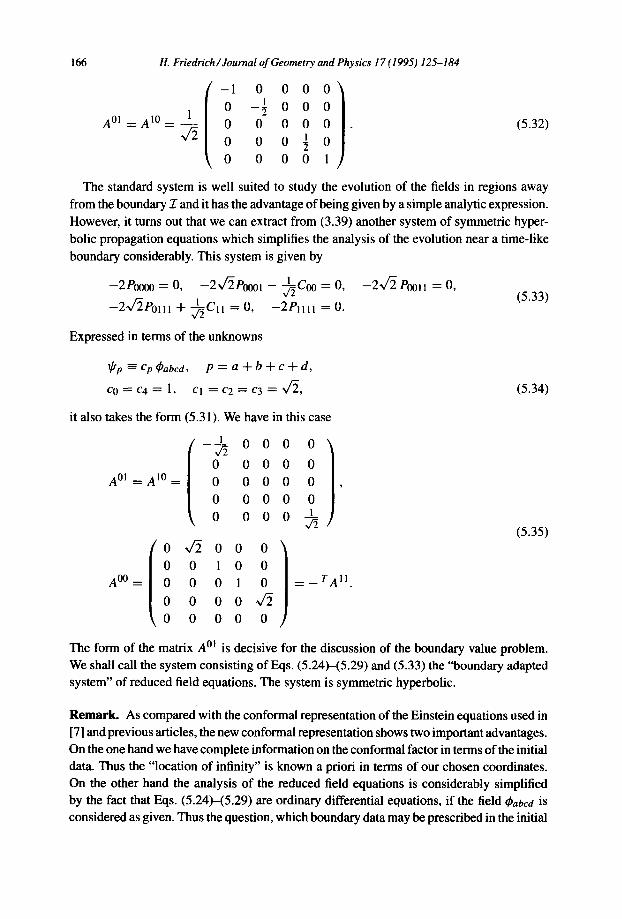
166 H. Friedrich/Journal of Geometry and Physics 17 (1995) 125-184
-1 0 000
0 AO’--to- - 1 i 0 fi (5.32)
0
0 0 001
The standard system is well suited to study the evolution of the fields in regions away
from the boundary Z and it has the advantage of being given by a simple analytic expression.
However, it turns out that we can extract from (3.39) another system of symmetric hyper-
bolic propagation equations which simplifies the analysis of the evolution near a time-like
boundary considerably. This system is given by
-2Poooo=O, -2JhKll- +o=o, -2&P~*l =o,
-21/2pom + hc,, = 0, -2P1,,, =O. (5.33)
Expressed in terms of the unknowns
$fp = cp #abed, p = a + b + c + d,
co=c4= 1, ct = c2 = c3 = 2/2,
it also takes the form (5.3 1). We have in this case
(5.34)
(5.35)
The form of the matrix A" is decisive for the discussion of the boundary value problem.
We shall call the system consisting of Eqs. (5.24~(5.29) and (5.33) the “boundary adapted
system” of reduced field equations. The system is symmetric hyperbolic.
Remark. As compared with the conformal representation of the Einstein equations used in
[7] and previous articles, the new conformal representation shows two important advantages.
On the one hand we have complete information on the conformal factor in terms of the initial
data. Thus the “location of infinity” is known a priori in terms of our chosen coordinates.
On the other hand the analysis of the reduced field equations is considerably simplified
by the fact that Eqs. (5.24)-(5.29) are ordinary differential equations, if the field C&cd is
considered as given. Thus the question, which boundary data may be prescribed in the initial
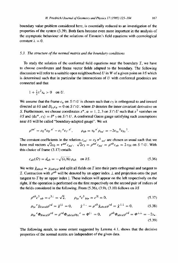
H. Friedrich/Journal of Geometry and Physics 17 (1995) 125-184 167
boundary value problem considered here, is essentially reduced to an investigation of the
properties of the system (3.39). Both facts become even more important in the analysis of
the asymptotic behaviour of the solutions of Einstein's field equations with cosmological constant ;. = 0.
5.3. The structure o f the normal matrix and the boundary conditions
To study the solution of the conformal field equations near the boundary 2, we have
to choose coordinates and frame vector fields adapted to the boundary. The following
discussion will refer to a suitable open neighbourhood U in W of a given point on OS which
is determined such that in particular the intersections of U with conformal geodesics are
connected and that
1 + l r 2 s , > 0 on U.
We assume that the frame Ca on S n U is chosen such that c3 is orthogonal to and inward
directed at 0S and D c 3 c a = 0 on S n U , where D denotes the inner covariant derivative on
S. Furthermore, we choose coordinates x a, u = 1,2, 3 on S n U such that x 3 vanishes on
0S and (dx '~, c3) = 3 a 3 on S n U. A conformal Gauss gauge satisfying such assumptions
near OS will be called "boundary-adapted gauge". We set
t a t a t p a a = EO a E o p - - E1 a ~ l r ,
t
Pab = ~:b a Paa' = --26"(a 06'b) 1
The constant coefficients in the relation Caa, = C k 0 "k aa' are chosen as usual such that we
have real vectors ~/2c0 = • a a ' c a a ' , ~ /r2c3 = aa' , p Caa = # a b c a b • 2 c01 on S n U. With
this choice of frame (3.17) entails
Cab(O) = dab = --V/~-/6) PaO on 0S. (5.36)
We write ) (abcd = X(ab)cd and split all fields on 2" into their parts orthogonal and tangent to
2". Contraction with pab will be denoted by an upper index _1_ and projection onto the part
tangent to 2- by an upper index I. These indices will appear on the left respectively on the
right, if the operation is performed on the first respectively on the second pair of indices of
the fields considered in the following. From (5.36), (3.9), (3.10) follows on OS
P abc3 ab = C31 = q ~ , P(a ec3 b)e = C3I = 0, (5.37)
P(a exb)ecdpCd = ~1-1- = O, ~ ± ± = pab~abcdpCd = )~±± = 0, (5.38)
P(a edpb)ecdpCd = tgcd(l~cde(aPb) e = ~1± --- 0, pabcl)abcdpCd = ~_l__k = --2S,.
(5.39)
The following result, to some extent suggested by Lemma 4.1, shows that the decisive properties of the normal matrix are independent of the given data.
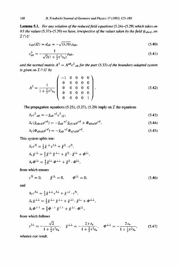
168 H. Friedrich/Journal of Geometry and Physics 17 (1995) 125-184
L e m m a 5.1. For any solution o f the reduced f ield equations (5.24)-(5.29) which takes on
O S the values (5.37)-(5.39) we have, irrespective o f the values taken by the f ield ~abcd, on
Z n U
Cab(~'2) = dab = - - ~ Pab, (5.40)
3 1 = - - I 2 . Pab, (5.41) Cab V'2(1 + ~r s , )
and the normal matrix A 3 = Aab c 3 ab f o r the part (5.33) o f the boundary-adapted system
is given on Z fq U by
I - 1 0 0 0 0
0 0 0 0 0 A3 - 1 0 0 0 0 0 (5.42)
1 + ½ r2s* 0 0 0 0 0
0 0 0 0 1
The propagation equations (5.25), (5.27), (5.29) imply on 2 the equations
Or c3 ab = --)(ab ef c3 ef ,
Or ()(abcdP cd) "= -- f(ab ef )(ef cdpCd -1- ~1) abcdP cd,
Or ( (i) abc d pcd ) = _ )(ab ef ¢i) ef c d pcd.
This system splits into
OrC31 = 1)~11 C3± -'1- )~11 . C31,
or21± = ½21± ;~-± + ~ , . ;~l- + ~l±,
o r a l ± = ½)~1± ~ ± 1 + )~11 . ~1±,
from which ensues
c 31 = O, )~11 = O, ~1± = O,
a n d
Orc 3± = ½ 2 ± l c 3± +2 ±1 .c31,
Or2±± = ½2±zi±± +2±1 .;~w± + ~ ± ± ,
Ores±± = ½~±±2±± + 2±1. ~1±,
from which follows
c3± _ x/~ l 1 + ~r2S.
whence our result.
~d_/ _ 2 r S ,
1 + 1 .t.2S, ' t~ -t--l- _
(5.43)
(5.44)
(5.45)
(5.46)
2 s,
1 + ~ "t-2s, (5.47)
H. Friedrich/Journal of Geometry and Physics 17 (1995) 125-184 169
In the following we will consider the initial boundary value problem for the boundary
adapted reduced field equations with data prescribed on S n U and 2- n U. The normal
matrix of the boundary adapted system is determined by (5.42). It follows that "maximal
dissipative" boundary conditions (cf. [9,19]) are described by a condition of the form
~111J - a ~ o o o o - c ~o'o'o'o' = d o n 2" n U
with complex-valued functions a, b on 2- satisfying
lal + Icl _< 1
(5.48)
(5.49)
and a complex-valued function d on 2. which represents the freely specifiable boundary
data.
Remark. The differences of the matrices A 01 in (5.32) and (5.35) and of the associated
normal matrices could suggest that the freedom to prescribe boundary data is larger for
the standard system of reduced equations. The uniqueness result for the solution of the
conformal field equations, which is based on the use of the boundary adapted system of
reduced equations shows that this cannot be true. The difference between the two types of
reduced systems shows up again in the discussion of the conservation of the constraints
near the boundary 2, where we obtain different systems of subsidiary equations in the two
cases. In the case of the standard system the discussion of the conservation of the constraints
would be quite involved. If we require that the constraints be satisfied, it should follow that
the freedom we have in prescribing boundary data for the standard systems is in fact the
same as that considered in the case of the boundary adapted system.
5.4. Comer conditions
Suppose we want to solve the initial boundary value problem for the conformal field
equations with data given on S and a boundary condition of the type (5.48). As is natural,
we will assume that the functions a, c on 2" have at least the smoothness which we want
to obtain for the solution. Given intial data on S near OS in the boundary adapted gauge
introduced in Section 5.3 and using the boundary adapted reduced field equations, we can
determine, up to a given order k which should be consistent with the smoothness properties
of the data, a formal expansion of the solution on S near OS in terms of the coordinate
r = x °. Restricting this expansion to OS we get in particular a formal expansion of the
function $1111 - - a ~/0ooo - c ~0'0'0'0', if we assume that a, c ~ C k (2"). It is then natural
to assume, that the free datum d in (5.48) is given as a function of the coordinates on 2-,
in particular of r, such that it allows a formal expansion up to order k in r and that this expansion coincides up to this order with the expansion of the left-hand side of (5.48)
(cf. the discussion in [9]). We will refer to this requirement as to the "comer condition of order k" and if the condition is satisfied to any order just as to the "comer condition". Given
C °° initial data on S and assuming that a, c E C ~ (2-), we obtain a formal expansion of the left-hand side of (5.48) to any order. Borel's theorem tells us how to construct functions d ~ C°°(2.) having the same formal expansion at OS. In the case of weak differentiability
170 H. Friedrich/Journal of Geometry and Physics 17 (1995) 125-184
there arise some subtleties with the corner conditions pointed out in [19]. We have no
reason to analyse these in this article. We shall show in Section 7 that we can prescribe
instead of the function d in (5.48) a smooth conformal structure on 2- as boundary datum.
Of course, in this case we also have to observe corner conditions. It is immediately seen
from the discussion in Section 7 how the corner conditions are to be expressed in terms of
the conformal structure and we will not discuss this any further.
6. The subsidiary equations
In the following we will consider solutions to the reduced field equations on some subsets
of S x [0, oo[. As before we identify S with S x {0} and 2- with aS x [0, oo[. The purpose
of this section is the proof of a "reduction lemma". For convenience it will be stated for
smooth solutions. By the way it will be derived it will become clear, however, that it remains
true also under weaker smoothness assumptions.
Lemma 6.1. (i) Suppose V is an open subset of S and U is an open neighbourhood of V in S x
[0, oo[. Assume the quantities (5.22) given on U represent a smooth solution of the
reduced equations (standard or boundary adapted)for data on V which satisfy the
constraint equations. Denote by g the metric for which the frame obtained from (5.22)
is orthonormal and by D+ (V) the future domain of dependence of V in U with respect
to g. Then the conformal field equations are satisfied on D+ (V) by the fields (5.22). (ii) Suppose p is a point in OS, U is an open neighbourhood of p in S x [0, oo[ and V is
the intersection of U with S U iT. Assume the quantities (5.22) given on U represent a
smooth solution of the boundary adapted reduced field equations for data given on V
in the boundary adapted gauge which satisfy on V N S the constraint equations (no
assumptions are made on boundary conditions on V f) Z). Denote by g the metric for
which the frame obtained from (5.22) is orthonormal and by D ÷ (V) the future domain
of dependence of V in U with respect to g. Then the conformal field equations are satisfied on D+ (V) by the fields (5.22).
6.1. Derivation of the subsidiary equations
The conformal field equations read
( ~ i , Cp /k Cq) = 0, ( A i k , Cp /NCq) -~- 0, (Ak, Cp A Cq) ~- 0, Aabcd = 0, (6.1)
where we assume the expressions
• 1 r ' ~ . ! i k ~ l j = ~azt l jkl a AOr 1, ,.-Qj : l ( - - d id i j k l ) t Tk AtY l --bi ff2ij
for the curvature forms, where
--2Aabcd -- PCbabcd -- 2 D f d ~abcdf --2(Pabcd -- 3 = ~ed(cCab)),
H. Friedrich/Journal of Geometry and Physics 17 (1995) 125-184 171
and where the functions £2, dk = £2bk are given by (5.10), (5.11) such that Eq. (3.55) is
satisfied which implies
bk + bo bk - ½rlok (b ib j - 2~.£2 -2) : 0. (6.2)
The reduced equations are given by
ico ,ui : O, ico Ai k = O, ico Ak = 0
and by PaOcd = 0 in case we use the standard system respectively by (5.33) if we use the
boundary adapted system. The reduced equations incorporate the gauge defined by
(t3ri,Ck) = ~ i k , (o.)ij,co) = 0 , (tOk, CO) = 0
and they are solved for data satisfying the constraint equations on S = {r = 0}. Conse-
quently the solution u = (c u k, Fi j k, fk, Fij, d i jkl) of the evolution equations satisfies all equations on S. To show that it also satisfies all equations in the domain of dependence
of S with respect to the metric g for which the frame ck is orthonormal, we derive a linear symmetric hyperbolic system of subsidiary equations for the quantities
(,~i, Cp m Cq), ( Ai k, Cp m Cq), (A k, Cp m Cq), p, q :~ O, Cab, (6.3)
and
where
Sk =- bk - f k - - £ 2 - 1 V k £ 2 ,
}/jk ~ Fjk -- Vjbk -- ½biS(b)j i k q- ~£2-2r]jk, S[pq], (6.4)
Spq = ['pq - - V p f q -- ½ fk S ( f ) p k q.
The fields (6.3), (6.4) will be called "zero quantities" in the following. It may be observed here, that the first two expressions in (6.4) may in principle be singular where £2 vanishes.
It will be seen however that this creates no problems with the uniqueness property required for the subsidiary system even in the case )~ > 0, where we have a time-like boundary. Since
the zero quantities vanish on S, we will be able to derive with the help of the subsidiary equations estimates which imply that the zero quantities vanish everywhere in the domain of dependence of S and the boundary 2-. This will show that in fact all conformal field
equations (6.1) are satisfied. We shall use the identity
( A i j , Cp A Cq) = r i jpq -- ( ~ k ; Cp A Cq)l-'k i j __ £2dijpq
-t~ i qSpj d- ~i pSqj - 6 i j(Spq - Sqp) q- llik (Spktlq j -- Sqkrlpj ),
where r i jpq is the curvature tensor defined by the connection coefficients/-]. J k (of which we do not know at the present stage whether they define a torsion-free connection) and the ck. This identity corresponds to the usual decomposition of the curvature tensor into its irreducible parts and Spq, which will be seen to be symmetric, represents the content of the
172 H. Friedrich/Journal of Geometry and Physics 17 (1995) 125-184
Ricci tensor of g. Finally it follows by (2.39) from ~k = 0, Yjk = 0, that the solution u will be such that the field Fjk derived from the metric ~ = S2 -2 g satisfies the equation
Fjk = Fjk -- ~rj (fk "[- A"2-1Vk ~('2) -- l ( j ~ --I- A ' 2 - 1 V i f f 2 ) S ( f "t- ~(2-1V~f2)j i k
q-•f f2-2gjk : 0, (6.5)
which implies that g is a solution to Einstein's vacuum field equations Ric[~] = )~ ~.
Denoting by L0 the Lie-derivative in the direction of co we get
L0(,~ 'i, Cp A Cq) : ILo ~, i , Cp A Cq) a t- (,E i, L 0 Cp A Cq) -I- (~ , i , Cp A L 0 Cq).
Using the reduced equations, the definition of A i k, and the fact that by the way we have
given ~(2 i j it satisfies the Bianchi identity (2.24), we obtain
Lo ,~i = (ico d + dico) z~, i = icod2? i = ico( Ai k A cr k -- 0.) i k A ,.,.Ek).
Observing that ico z~'i ~--- O, we finally get for p, q = 1, 2, 3
L0 (/7i, Cp A Cq) = (A i 0, Cp A Cq) -- (.~i, c I A Cq)((.o I 0, Cp)
- ( I ? i, Cp A c l ) ( J 0, Cq). (6.6)
By similar arguments we derive for p, q = l, 2, 3
LO ( Ai k, Cp A Cq) = - - S ( ( A I , Cp A Cq))Oi k -- ( A i k, CO A Cp A Cq)
- - (o) lo , c p ) ( A i k , C I A C q ) -- (o)lo, c q ) ( A i k , C p ACl ) , (6.7)
LO ( Ak , Cp A Cq ) : --( Ak , cO A Cp A Cq ) -- (0) I 0, Cp) ( Ak , Cl A Cq )
--( (-0l 0, Cq) ( Ak , Cp A Cl) , (6.8)
where
and
Ai k ---- d 57i k -- ff2i j A 09 j k -t- O) i j A if2 j k @ S(ff21)j i k A t7 j
Ak =dY2k -- O j AO)J k q-O)j AA'2J k .
By straightforward calculations we find
A i j ---- ff2d i j p q ~ P A t7 q --J- [ l f f 2 Vm dm stkEj itkErpq s
q-•m(d mi pqlTrj - dmjpqr~ i r ) ] o'r A O "p A o "q,
and
A k = - b j A j k -~- Yij tTi A t'2 j k.
(6.9)
The right member of the first of these two equations, whence also the right member of the last equation, can he expressed as a linear expression of the zero quantities. It follows that also the right members of Eqs. (6.6)-(6.8) are linear in the zero quantities.
(6.1o)
H. Friedrich/Journal of Geometry and Physics 17 (1995) 125-184 173
We know already that 80 = 0. The gauge conditions and Eq. (6.2) imply that ?'Ok ---- 0. It follows directly from the definitions and the gauge conditions that
fToSp = gpo - f'p j 06j, p = 1, 2, 3, (6.1 i)
and, using Eq. (6.2),
VOYpk = --)lqk l~p q 0 -- bOYpk -- bk YpO + Ook (b j }/pj - 2~.j2-2 (~a) (6.12)
for p = 1, 2, 3 and k = 0, 1,2, 3. Using again the propagation equations we derive
*OSlpq] = 1 ( ( A o , c p ACq) q- f i ( A i o , cp ACe) )
- t - l (Fp l 0(A j j , C I A Cq) -- Fq l o (AJ J' Cl A Cp)). (6.13)
The derivation of the equations for Cab is similar to that given in [71. Writing
Hijk = 7p dp kij
in terms of spinors and decomposing into irreducible parts, we get the identity
d t - Haa'bb'cc' = - - rd c' Aabcd 6a'b' -- rc Aa'brc'd ' Eab
= - - r d c'(Pabcd 3 -- -~ 6 d(cCab) )6a'b
' - _ 3 ~ ~ , . --rc d (Pa'b'c'd' ~ed (c't~a b ))eab. (6.14)
This implies the further identity
_ 3 PCab - ~(a CCb)c "1- 2 ~)ef Pabef d- 2~df2X b h eh (Pcdbe ~Ee(bCcd))
= 2 V cc' Aabcc,. (6.15)
On the other hand we get by a direct calculation which uses the symmetries of dijkl
v k Hijk : dllj kP ( Al i], Ck A Cp) -- dij IP ( AI k, Cp A Ck )
q--I (~'k, Cq A Cp)Tqdi j kp q_ dplijs[pll. (6.16)
From (6.14) to (6.16) follows the equation for Cab, the right member of which is again linear in the zero quantities. That the equation is symmetric hyperbolic is seen immediately in the case, where the standard system has been used for the evolution. In this case (6.15) reduces
to
CCt t . PCab -- D(a CCb)c -- -~2 Xe d fd~f(aCbe) : 2V Habcc
In case the boundary adapted system has been used for the propagation, Eq. (6.15) can be written in the form
P Coo + DooCol = Uoo, P C01 + DooCll -- DI1COO = U01, P Cl l - D11Col = Ul l (6.17)
with linear functions Uab of the zero quantities.
174 H. Friedrich/Journal of Geometry and Physics 17 (1995) 125-184
Eqs. (6.6)-(6.8), (6.11)--(6.13), (6.15), with the right-hand sides written as linear expres- sions in the zero quantities as explained above, constitute the system of subsidiary equations.
It is an important property of this system that Eqs. (6.11), (6.12) decouple from the remain- ing subsidiary equations and form a linear system of ordinary differential equations. Since the zero quantities vanish on S, the functions ~k, Yjk vanish on the set {~2 > 0}. The re-
maining part of the subsidiary system then has coefficients which extend continuously to 2". It is symmetric hyperbolic and its cone of characteristic rays is inside the null cone defined
by the metric g. This implies, irrespective of the sign of ~., that the zero quantities vanish
in the domain of dependence of a given subset of S with respect to the metric determined by the solution of the reduced equations. Thus the conformal field equations are satisfied
in that region. Near a time-like boundary as represented by 2" the argument is slightly more
involved.
6.2. Conservation o f constraints near a time-like boundary
In case the boundary adapted gauge and system of reduced equations have been used
to propagate the fields near the boundary 2-, the subsidiary equations can be written with respect to conformal Gauss coordinates near a given point on aS in the form
F ~ V u u = G u,
where V is the Levi-Civita connection for g and F u, G are matrix-valued functions such
that the F u are hermitian, F u V u x ° is positive definite near OS, and, as follows from (6.17)
and Lemma 5.1, the normal matrix of the subsidiary system satisfies the decisive condition
F 3 = 0 on Z fqH. (6.18)
Furthermore, we find that
det (FU~u) = (ru~#) p ((r#~u) 2 -4- 2~00~11) >_ (r#~u)P gUV~u~v
with some positive integer p. Let now t > 0 be a smooth function defined in the neighbour-
hood U of OS where we solved the boundary adapted reduced equations. We assume that each level set of t intersects S as well as 2- in space-like surfaces, that these intersections approach a closed subset of 0 S as the function t approaches 0, and that the gradient of t with respect to the metric obtained from the solution to the propagation equations is time-like
and lies in a compact region of the interior of the future null cone. For a 6 R, a _> 0 we set Ta = {p E M I t ( p ) = a } , Va = {p 6 M l O < t (p ) < a} and la = 2-N Va, Sa = S N V a. Fix a small A > 0. Integrating VtL (t ~ F u u) = t fi H u with H = t ~ + G + Vu FU over Va
for a ~]0, A], observing (6.18), our assumptions on the function t, and the fact that u = 0 on Sa, we get after a partial integration
f n u ( t ~ F # u ) d S a = f ( t ~ H u ) d l z g < C i ( f n u ( t F ~ F t Z u ) d S s ) d s ,
Ta Va 0
H. Friedrich/Journal of Geometry and Physics 17 (1995) 125-184 175
where C >_ 0 is a constant which does not depend on a, dSs denotes the volume element
induced on Ts by g, and n u is the future directed unit normal to Ts. Gronwall 's lemma
implies now, that u = 0 on Va, which we wanted to show.
7. Covariant boundary conditions
The discussion in Section 5 suggests looking for solutions of initial boundary value
problems for the conformal field equations where the boundary data are given in the form
(5.48). It appears, however, that boundary conditions of this general form are not suitable
for geometric discussions. On 2- the frame vector field c3 -- n normal to the boundary
is singled out naturally. We have prescribed initial conditions for the conformal geodesic
curves everywhere on S, which fix in particular the time-like vector field co on 2-. Rotations of
the frame on 2- which leave the normal vector and the time-like vector field on 2- unchanged
are given by Caa, --~ e(a'-a)i¢Caa ,. Under these rotations the components of the rescaled
Weyl spinor transform according to ~tabcd ~ e (2 -k ) i~abc d with k = a + b + c ÷ d. Thus
the boundary condition (5.48) and condition (5.49) can only be given an invariant meaning under such transformations if we require the transformation behaviour a ~ e-4i~a, c
c, d --~ e-2ieVd. We shall restrict ourselves to boundary conditions, where the functions a,
c are constant. This is only sensible, if we assume that a vanishes. Thus we shall consider
boundary conditions of the form
1/fl111 - - C l~lY0'0 ' 0 ' = d , c = cons t . , Ic l < 1. (7.1)
Note that the assumption, that the data correspond to fields given in a boundary adapted
gauge, is part of their specification. In general there does not exist a boundary adapted gauge
in a complete neighbourhood of 0S in which the quantity d could be given. Therefore it
is important that the transformations of d under changes of the boundary adapted gauges
are controlled in terms of the changes on 0S. Consider in a fixed boundary adapted gauge
the function d = d(r , x 1, x 2) along a given conformal geodesic on 2- which is specified
by the values of the coordinates x I , x 2 at points of OS. A change to another boundary adapted gauge implies a change of the frame field Cad ~ e (a'-a)i@(xl'x2)caa, on OS. As a
consequence of the conformal geodesic equation (cf. (2.41)) this entails the transformation d(r , x 1 , x 2) ~ e-2i~(x~'x2)d(r, x 1, x2), i.e. the phase factor remains constant along the
geodesic. Thus d has to be given as a spin weighted quantity on 2- which has a transformation
law that is correlated to transformations of the data on S as described above.
Still, there is no obvious way to compare such boundary conditions for different choices
of the frame if the field co, which in general cannot be fixed by a natural requirement, is
also changed. In the following we shall study an example of a boundary condition, which
has a covariant meaning.
7.1. Boundary conditions in terms o f fields on 2-
We assume again that n = c3 is the inward pointing unit normal on 2- and use the spinor
176 14. Friedrich /Journal of Geometry and Physics 17 (1995) 125-184
f a ~ paa ~ 60aEora _ El aE1 ~
to project fields into 2" in analogy to the splittings we performed with respect to the time-like b' spinor r aa'. We set tab : Pb tab' = 2 e(a Oeb) I. The n-magnetic and n-electric parts of
the rescaled Weyl tensor daa'bb'cc'dd' = qbabcd ea'b' ec'd' + C~a'b'dd' eab ecd, which represent
tensor fields in 2", are given by
nabcd : l pba'pee'pdC' f f ' ' * : - - l i(~abcd -- qgabcd P aaa'ee~cc~ff
respectively
t t d -
Eabcd = l pb a'pee'pd c p f f daa,ee,cc,ff ' : l (q~abc d _]_ qbabcd),
where the star denotes again the four-dimensional dual and
t~aq-b a' b . . . . c d cd ~ Pa Pb Pc Pd ~)a'brc'd '
the p-conjugated of ~abcd. The magnetic part admits a decomposition
Babcd ~ babcd q- bab ~'cd "-I- "Cab bcd d- 1 b (3~:ab~:cd -- 2ea(c Ed)b),
where
babcd ~ b(abcd), ~'abbabcd = O, bab = b(ab), ~abbab = O, b =/~.
A similar decomposition is obtained for the electric part. The spinor field babcd on 2-, which
represents the trace free part of the projection of the magnetic part into the space orthogonal
to r aa', has as non-vanishing components only
bl l l l ~- - l i (q~ l l l l - ~0'o'0'o') = BIIl l
and b0ooo, which is the complex conjugate of bil l I. Also bll = - ½i (~b0111 -- ~1'0'0'0') is
the complex conjugate of boo, bol = 0, b = - i (q~ooll - q~vvo'0'). Similarly the field eabcd
is completely represented by the component el ll~ = ½(4~1111 + ~0'0'0'0') = El ll2. From this we find that some of the boundary conditions (7.1) can be expressed with respect to
tensor fields in 2-. In case c = 1 condition (7.1) can be replaced by
Blil l = d, (7.2)
while in the case c = - 1 we can write
El l l l = d (7.3)
with suitable data d. To relate such boundary conditions given with respect to different choices of co, we try
to exploit the special properties of the conformal boundary. We assume that we are given a solution of the conformal field equations which is such that either condition (7.2) or
condition (7.3) is satisfied with some given function d on 2-. We denote by Dab, T, and • . a !
~ab the inner covariant derivative on 2" in the direction of P(b Ca)a', aa' , and "~ C a a "~(a e Cb)e
respectively, such that we have Dab = ½tab T + 8ab. We know then from (4.11), that
H. Friedrich /Journal of Geometry and Physics 17 (1995) 125-184 177
Dab Babcd = O, D ab Eabcd = 0 o n 2-. Using the expansions above f o r Dab a n d Babcd, w e
find that the first of these equations is equivalent to
! T b + ($abbab ~ 1 bab T T ab -- 3 - ~ a b 2 ~ 0 13 l;ab "k lrefDabbabef, (7.4)
2 T bcd + 3cdb = 2(bcd D e f r e f q- be f Defrcd)
3 b T rcd+ (2ec e 6d f _~_ rcdref) Dabba6e f (7.5) 2
For given babcd, i.e. for given datum (7.2), we can read these equations as partial differ- ential equations for the fields ba¢, b. The principal part of the system is given explicitly by
writing the system (7.4), (7.5) in the form
-c~' I, 2 r u 0 Ou boo = f l ,
--C~0, 0 2 r/z bll f2
t
where r r' = z "aa c # aa' and the right-hand side depends linearly o n bac, b and on the "source t e r m " Dabbabef. Thus the equations form a linear symmetric hyperbolic system.
We could use it to determine Babcd on 2- from known data on 0 S and the boundary data (7.2) if we knew the interior metric on 2-. We could then compare boundary conditions
given with respect to different gauges. A similar statement is true for the electric part of
the rescaled Weyl tensor. There is a basic difference between the electric and the magnetic
part. By (4.11) the magnetic part Bahia is essentially given by the Cotton tensor of the interior metric h on 2-. This offers a possibility to relate the data (7.2) to the metric h. The following result, expressed in terms of the notation used in Lemma 6.1, allows, to express
the boundary conditions purely in terms of the interior conformal structure on 2" which is not subject to any constraint except the requirement that corner conditions be satisfied.
Lemma 7.1. Suppose the fields (5.22) represent a solution of the conformal field equations
with cosmological constant ~ > 0 on S x [0, a[, a > O,for which 2- = O S × [0, a[ represents
the conformal boundary at space-like and null infinity, g denotes the metric for which the
frame supplied by (5.22) is orthonormal, and h is the interior metric induced by g on 2-. We
assume that the gauge considered in Section 5 can be extended to all of S × [0, a[.
(i) If we know on aS the data implied by (5.22) in the boundary adapted gauge and if
we know the conformal class of h on 2-, we can calculate on 2- the datum (7.2) with
respect to the gauge considered in Section 5.
(ii) Conversely, given on OS the data implied by (5.22) and on Z the data (7.2), both
in the conformal gauge considered in Section 5, the conformal class of h on 2- is determined uniquely as a solution of a quasi-linear symmetric hyperbolic system of
partial differential equations on 2-.
To show (i) we recall that by Lemma 4.1 the gauge can be determined on 2- for given data on a S by solving the conformal geodesics equations defined by the interior conformal structure of 2-. With respect to this gauge we can calculate the Cotton tensor, which by
178 H. Friedrich/Journal of Geometry and Physics 17 (1995) 125-184
(4.11) determines the magnetic part of the rescaled Weyl tensor on 2". From this we can read off the desired datum (7.2).
The demonstration of the second part is more complicated. In dimension n = 3 the curvature of the normal conformal Caftan connection is represented by ~2j alone, since
by (3.18) a trace free tensor possessing the symmetries of a curvature tensor vanishes. It
follows then from (2.32) that Kjkl has a tensorial transformation law under transformations
t ~ H ( p , q). This tensor, the Cotton tensor, vanishes if and only if the conformal structure can locally be represented by a flat metric. All algebraic properties which are obtained if Kjkl is represented with respect to the Levi-Civita connection V of a metric g hold in any
representation. In addition to its antisymmetry in the last pair of indices and the property (2.30), it satisfies K i il ~-" O. If ~ijk denotes the totally antisymmetric Levi-Civita symbol
with respect to g we have a representation
K j k l -~- K j i Ei kl
with a symmetric and trace-free tensor field Kji . We consider the system
0 : ~,i ~_ dtTi d- o~ i k A O "k, (7.6)
0 : A i k ~ d toi k -~ o)i l A o) I k - - S (o )p )q i k A t7 q , (7.7)
0 = Ak -- dwk + o)i A CO i k - - ~)k, (7.8)
0 = A j -- d ~ j - E2k/x w k j , (7.9)
provided by the structure equations and the fourth Bianchi identity (2.31).
We want to determine a frame field cj, j = 0, 1, 2 on 2" which coincides on 0S with the frame supplied by the data and satisfies the gauge conditions
( a i , C k ) : t~ik, (O) i j , C 0 ) : 0, (O)k, C0) : 0,
which by Lemma 4.1 corresponds to the gauge used in Section 5. Writing E2j = 1 Kj i t i kltTk A
t7 t, we evaluate the system
ico E i =- O, ico Ai k : - O, ico Ak = 0, A j = O, (7.10)
in terms of the frame cj and coordinates x ~, t~ = 0, 1, 2, satisfying (dx ~, co) = 8~, x ° = 0
on 0S. The first three of these equations involve only the derivative operator co. The last equati6n takes in terms of the Levi-Civita connection V of the metric for which the frame cj is orthonormal, the form
0 = V i Ki j . (7.11)
By (4.11) certain components of the tensor field K 0 can be expressed by the data (7.2). After these components have been given, the system obtained from (7.10) constitutes by (7.4), (7.5) a symmetric hyperbolic system. Given the data on aS, the (unique) solution of this system (cf. [20]) close to OS determines the conformal structure on 2". In fact, we get the frame in the gauge considered in Section 5. By arguments similar to those used in the
1t. Friedrich/Journal of Geometry and Physics 17 (1995) 125-184 179
derivation of the subsidiary system it follows that the forms cr i, w i k, toj, I21 supplied by
the solution to (7.10), which satisfy (7.6)-(7.9) on 0 S, satisfy in fact (7.6)-(7.9).
7.2. Description o f the boundary data in terms o f the metric ~,
Conformal geodesics allow a convenient description of the covariant boundary condition
studied above in terms of fields directly related to the metric ~. We begin with a few obser- vations concerning conformal geodesics in terms of the metric ~ which satisfies the Einstein equation (3.1). Suppose that x ( r ) , b ( r ) , ck ( r ) are as in Lemma 3.1. We reparametrize these
quantities by the arclength tr of x ( r ) with respect to ~ and write 4 -- (dx/dtr ) = ~tf,
t9 = 69 f , etc. We can assume that f = O and we have along the conformal geodesic
~7~4 -- y (7. ! 2)
with some vector field y orthogonal to 4, which satisfies by Eq. (2.49)
b = y + ( 9 4 = y + (b, 4)4. (7.13)
From this and Eq. (2.50) follows Viy = - ~ ( y , y) 2, which entails that ~(y, y) is constant along the conformal geodesic. Since :t is time-like, there can occur two cases. I f b is propor- tional to ~t at one point it remains so and the conformal geodesic is up to a reparametrization
a metric geodesic. If y ~ 0 at some point, this property will also be preserved and x ( a ) is
a curve of non-vanishing acceleration y. Setting ak = 09 ck, we obtain a frame which is orthonormal for ~. It satisfies by (2.51 )
the equation fTiak = -- (b, ak )4 + (ak, 4)b which, in view of (7.12), (7.13), can be rewritten in the form V~ak + ~(4, 4){g(ak, V¢4)4 -- g(ak, 4)V$4} = 0, showing that the frame ak is Fermi-transported. It follows that the coefficients x k, yk of the expansion 4 = xkak, y =
ykak are constant along the conformal geodesic. We write now O = I2 and describe our gauge conditions in terms of x(cr), y(tr), the
conformal factor ~2 and its differential dl2 on S, which is known by (5.4). The smooth congruence of conformal geodesic curves in AT/is obtained by solving the equations
~'~4 = y, ~'~y = - ~ ( y , y ) 4 ,
with initial conditions x(0) ~ S, 4(0) is future directed and orthogonal to S, ~(4(0), 4(0)) = 1, yU(0) = (b tz - ~2A~)ls = ~ - l ~ , " v V v I 2 on S. It follows that ~(4, 4) = 1, ~(4, y) = 0, ~(y, y) = const . = -½~. + 2 $2. s. along these curves in/17/. For co ~ N,
0 < w << 1 the set S~o = {£2 = o9} defines a smooth hypersurface in S near space-like in-
finity. The conformal geodesics starting from S~o generate a smooth time-like hypersurface To) i n / f / n e a r S. We denote the metric induced by ~ on To) by h,o and the function induced by $2 on T,o by ~2,o. Then the boundary data given on 2? are apparently represented by the
2 ~ conforrnal class of the metric which is obtained as a limit h = limbo--,0 $2o)h~o. Care must be taken here with the limit procedure. A point p on To, is parametrized by the point p' where the conformal geodesic through p meets S,o and by the value at p of the parameter cr on this conformal geodesic. We require that the limit is taken along the curve, for which
1 8 0 H. Friedrich/Journal of Geometry and Physics 17 (1995) 125-184
p ' follows the flow generated by the field y on S and for which the value of the parameter
r = r (tr) is constant. From (5.10) follows that the parameter r is related to the parameter
tr by
d r ' ~ ' 2 , O" = - - .
1 -- l•t2S, 0
This equation determines the way in which we have to let ~r go to infinity in order to achieve
a limit with constant value r > 0. Along any such curve we consider for a given value of
o9 the set of future directed null vectors N of h~o satisfying the normalization condition
ho,(~, N) = 12o~ 1. In suitably chosen coordinates these sets define limiting null cones
which in turn determine the conformal structure on 2".
8. Existence results
The reduced conformal field equations will be used now to prove Theorem 1.1. We shall
adopt the notation used in Theorem 1.1. The unknowns in the reduced field equations will
be denoted in the following collectively by the "column vector"
U = (CIZ ab, ["abcd, ~l)acbd, l~racbd). (8.1)
We assume that (3, h, )~) is a smoothly conformally compactifiable Cauchy data set for
the Einstein equations (1.1) with positive cosmological constant )~ > 0. As described in
Section 5.1 we can derive from it the data for the fields comprised by u. We assume that these data extend smoothly to S and denote them collectively as u0. We assume furthermore
on 2" = OS x [0, oo[ a smooth spin weighted field d which is defined with respect to any
boundary adapted gauge of the data u0 on S such that the correlation of the transformation
laws for the data on S and of d hold as described in Section 7. Finally we assume that
the data u0 on S and d on 2" satisfy the comer condition discussed in Section 5.4. When
we use the reduced field equations there remains the freedom to choose the frame and the
local coordinates on S. Observing the remarks following (5.8) and (5.9), we note that the
function x ° = r will be independent of this choice and depend only on the metric g on S
and on the conformal structure defined by the solution g of the conformal field equations which we want to construct. This allows to identify the function r with the projection of
M = S x [0, c~[ onto [0, ~x~[. We will now prove a result which is somewhat more general than Theorem 1.1. Observing Lemma 7.1 it is easily seen that the following theorem entails Theorem 1.1.
Theorem 8.1. Suppose we are given data uo on S and d on Z as described above and a
complex number c with Icl <_ 1. Then there exists fo r some a > 0 a unique smooth solution
u o f the conformalEinstein equations (3.33) on Ma = {p ~ M [ 0 < r ( p ) < or} with
the properties: (i) on S the data uo are induced by u, (ii) the boundary condition (7.1) is
satisfied on Z A Ma, (iii) in a local gauge and in conformal Gauss coordinates as described
H. Friedrich /Journal of Geometry and Physics 17 (1995) 125-184 181
in Section 5.1, the fields I-2 and dab in (3.33) are given by (5.10), (5.23), and r is a parameter
o f the conformal geodesics.
The uniqueness of the solution can be deduced from the uniqueness properties of our
gauge conditions and from well-known properties of symmetric hyperbolic systems. We shall not further comment on it.
Due to the hyperbolicity of the equations this problem can be localized. Given the restric-
tion of the data u0 to an open subset V C S on which the local gauge described in Section 5.1 can be defined, it follows from well-known results on symmetric hyperbolic systems (cf. [201) that there exists on a certain neighbourhood U of V in M a unique solution to the reduced field equations (5.24)-(5.30), which takes the given values on V. By Lemma 6. !
this is in fact a solution to the conformal field equations given in the gauge of Section 5.1 and with I2 and dab given by (5.10), (5.23). Suppose we can show the existence of a unique local
solution in an open neighbourhood U in M of a given point p E OS to the mixed problem for the boundary adapted system of reduced field equations, where the initial data are given by the restriction of u0 to V t = S M U and the boundary conditions (7.1) hold on V n = Z N U.
Again by Lemma 6.1 this solution solves in fact the conformal Einstein equations. The local
solutions so obtained can be patched together if their initial data are given on intersecting
domains (cf. [7]). Since S can be covered by a finite number of local solutions we obtain as the result of the patching procedure a solution as described in Theorem 8.1.
This reduces the proof of Theorem 8.1 to the discussion of the local mixed problem. We assume that in a neighbourhood V' of the point p ~ OS in S the data are given in a fixed boundary adapted gauge such that xU(p) = 0 and that r --- x °, x 1 , X 2 are coordinates on V n. The neighbourhood U of p is thought of as being embedded via the coordinates onto
an open neighbourhood of the origin in •4. We reformulate now our problem as a mixed problem, where the equation is a real equation of the form
AUOuu = F(a, Ova, u) on N~ = {x c ~4 [0 < X 3, 0 < X 0 < ~} (8.2)
for an R u-valued unknown u. Here a denotes an ~N'_valued function of compact support in {x E R41x °, x 3 > 0}, A u = AU(a, u) are smooth, symmetric, N × N-matrix-valued functions of (u, a) such that A°(a, u) is positive definite for u ~ R iv and F denotes a
smooth R u-valued function. The boundary conditions are of the form
B u = 0 on{x 3 = 0 , 0 < x 0 <t~} (8.3)
with a constant real 2 x N matrix B of rank 2, and the initial condition is
u = 0 on{x 3 > 0 , x ° = 0 } . (8.4)
This formulation is obtained by going through the following steps, where we assume for simplicity that ~t = cxD:
(i) The part of the boundary adapted reduced field equations (5.33) has the form
(I + A°)Or¢ + A~Oa ¢ = B(F, ak)
182 H. Friedrich /Journal of Geometry and Physics 17 (1995) 125-184
with A u = A ab c u,//, : 0, 1,2, 3. We replace in this equation A ° by AabCab where
the smooth map Cab = Cab(C ° ca), defined for fields c o ab satisfying the usual reality
conditions, is constructed as follows. We choose smooth real functions f01, f lo on
the real line and complex functions fo0, f l I on the complex plane, all with compact
support and such that f01 = fl0, fl l(Z) = - f 0 o ( - z ) , fab(Z) : Z for IZl < y' and Ifab(Z)l <_ r' with certain constants y > y ' > 0. For fixed indices ab the map Cab is assumed to depend only on c O ab such that Cab(C ° ca) = f ab ( C 0 ab ). Then Cab = c o ab
for [cOabl < y ' , ICabl <_ y , and the matrix A~bCab is hermitian. We choose the constants y, y ' such that I + AabCab :> ½I. Observing that the data for cOab vanish
on {r = 0}, we see that the new equations are equivalent to the old equations in regions where IcOabl < y ' .
(ii) We choose a function q ~ C~(R , R) with q ' < 0, q(s) = 1 for s < 1, q(s) = 0 for
s > 2 and define qc E C ~ ( R 4, R) by qe(x) = q ( I x l / e ) with some e > 0 such that
3 I x E ~ 4 t x O , x 3 > O } O s u p p q 4 E C V ' x [ O , oo[, 1 _< 1 + ½r2s,(xa) < ~
for (r, x '~) ~ supp q4~. (iii) Wechooseon V'x[0 , ~x~[acollectionvofsmoothfieldsanalogoustothoserepresented
by u which satisfy the boundary condition (7.1) on 2" = 2" N (V' × [0, c¢[), which coincide with the data u0 on V', and for which the respective components take on
2"~ f3 supp q4E the values (5.46), (5.47). (iv) In the part of the boundary adapted reduced field equations given by (5.33) we replace
the term A 3 = Aabc3 ab by Aab(qec3 ab -{- (1 - - qe)eab) with eab = - - P a b / q f~ =
c 3 ab[OS = const .
(v) After this we replace in all equations u, I2, and dab respectively by u + q2~v, q2Ei2,
q2Edab and denote the functions qe, q2e v, q2~ I2, q2edab in the equation collectively by a. We extend these functions by value zero to {x E ~4 ix o, x 3 > 0} to obtain smooth functions of compact support in {x ~ ~41 x°, x3 ~ 0}.
(vi) Observing the reality conditions which are to be satisfied by the various components of the fields comprised by u, we finally write the resulting equations as a real symmetric hyperbolic system for an RN-valued unknown which we denote again by u. The R N'-
valued function appearing in the equations will again be denoted by a.
We have reformulated the problem in such a way that there exists a neighbourhood of the point x u = 0 in {x ~ ~4 i x 0, x 3 < 0} on which the original problem is equivalent to the initial boundary value problem defined by (8.2)-(8.4).
The reformulation shows that our problem is close to a class of problems discussed by Guts [9]. In fact, we have achieved almost the same form of the problem as considered in that article. There is a slight but important difference. In the article by Guts it is assumed that the basic properties of the normal matrix A 3 are determined on {x 3 = 0, x ° > 0} by the boundary conditions. In the present case the normal matrix is determined by Eq. (8.2). However, we have perfect control on it. By Lemma 5.1 the normal matrix can be deter- mined by integrating the system of ordinary differential equations (5.43)-(5.45). After our reformulation we find that the normal matrix in Eq. (8.2) is essentially given by
H. Friedrich/Journal of Geometry and Physics 17 (1995) 125-184 183
l-t-2s, A 3 ( a , u ) = f ( x ~ ) A 3 on{x 3 = 0 , x 0 > 0 } , f = l - q E (8.5)
1 + l r 2 s , '
where we denote by A30 the value of the matrix (5.42) at r = 0. It follows that f is a smooth
function satisfying 2 < f < 2 on {x 3 = 0, x ° > 0}. If one studies, following the procedure
in [9], in an iteration procedure the sequence of linear problems
AN(a, Uk)Oi~Uk+l = F(a, Ova, uk), k = 1, 2, 3 . . . . (8.6)
for an unknown Uk+l, where the iteration is started with the function ul which vanishes
everywhere, it follows for any k, that the normal matrix of Eq. (8.6) is given by (8.5).
Consequently every step in G u t s ' discussion can be applied to the present situation. Since
for the situation considered here nothing can be gained in the smooth case which would go
beyond the results obtained by Guts , we refrain from repeating the details. Theorems 3 and
4 in [9] imply the following theorem.
Theorem 8.2. There exists a numberct> 0 for which there exists a unique smooth solution
u of the problem (8.2)-(8.4).
We could deduce from [9] a result involving weaker differentiability assumptions. It
should be noted that the smoothness results near the boundary obtained for the general case
studied in [9] may then be slightly improved for our particular problem.
Finally, we want to point out that the extensibility Theorem 4 in [9] is only of restricted
applicabil i ty in our situation. On the one hand we know from the discussion in Section 4.1
that even if the solution considered above would exist for arbitrary values of the coordinate
r , the solution might still be extensible after a coordinate transformation. On the other
hand it may happen that some of the fields considered in our representation of the field
equations blow up after a finite "time" r because the conformal geodesics form caustics,
while the underlying space- t ime might still be extensible as a solution to the conformal
field equations.
References
[ 1 ] L. Andersson and ET. Chrugciel, On the asymptotic behaviour of solutions to the constraint equations in general relativity with "hyperboioidal" boundary conditions, preprint (1994).
[2] L. Andersson, P.T. Chrugeiel and H. Friedrich, On the regularity of solutions to the Yamabe equation and the existence of smooth hyperboloidal initial data for Einstein's field equations, Commun. Math. Phys. 149 (1992) 587-612.
[3] E. Cartan, Les espaces h connexion conforme, Ann. Soc. Po. Math. 2 (1923) 171-221. [4] Y. Choquet-Bruhat and J.W. York, Jr., The Cauchy problem, in: General Relativity and Gravitation,
Vol. I., ed. A. Held (Plenum Press, New York, ! 980). [5] H. Friedrich, On the existence of n-geodesically complete or future complete solutions of Einstein's
field equations with smooth asymptotic structure, Commun. Math. Phys. 107 (1986) 587-609. [6] H. Friedrich, On static and radiative spacetimes, Commun. Math. Phys. 119 (1988) 51-73. [7] H. Friedrich, On the global existence and the asymptotic behaviour of solutions to the Einstein-
Maxweil-Yang-Mills equations, J. Diff. Geom. 34 (1991 ) 275-345.
184 H. Friedrich /Journal of Geometry and Physics 17 (1995) 125-184
[8] H. Friedrich and B.G. Schmidt, Conformal geodesics in general relativity, Proc. Roy. Soc. Lond. A 414 (1987) 171-195.
[9] O. Gu~s, Probl~me mixte hyp~rbolique quasi-lin6aire charact6ristique, Commun. Part. Diff. Equ. 15 (1990) 595-645.
[10] S.W. Hawking, The boundary conditions for gauged supergravity, Phys. Lett. 126 B (1983) 175-177. [11] S.W. Hawking and EG.R. Ellis, The Large Scale Structure of Space-lime (Cambridge University
Press, Cambridge, 1973). [12] M. Henneaux and C. Teitelboim, Asymptotically Anti-de Sitter spaces, Commun. Math. Phys. 98
(1985) 391-424. [13] S. Kobayashi, Transformation Groups in Differential Geometry (Springer, Berlin, 1972). [14] K. Ogiue, Theory ofconformal connections, Kodai Math. Sem. Rep. 19 (1967) 193-224. [15] R. Penrose, Conformal treatment of infinity, in: Relativity, Groups and Topology, Les Houches 1963,
eds. B. de Witt and C.M. de Witt (Gordon and Breach, New York, 1964). [16] R. Penrose, Zero rest-mass fields including gravitation: asymptotic behaviour, Proc. Roy. Soc. Lond.
A 284 (1965) 159-203. [17] R. Penrose, Structure of space-time, in: Battelle Rencontres, 1967 Lectures in Mathematics and
Physics, eds. C.M. de Witt and J.A. Wheeler (Benjamin, New York, 1968). [ 18] R. Penrose and W. Rindler, Spinors and space-time, Vols. I, II (Cambridge University Press, Cambridge,
1986). [19] J. Rauch, Symmetric positive systems with boundary characteristics of constant multiplicity, Trans.
Amer. Math. Soc. 291 (1985) 167-187. [20] M.E. Taylor, Pseudodifferential Operators and Nonlinear PDE (Birkh~iuser, Boston, 1991 ). [21] H. Weyl, Reine Infinitesimalgeometrie, Mathem. Zeitschrift 2 (1918) 384--411. [221 K. Yano, Sur les circonf&ences g6n6ralis6es dans les espaces h connexion conforme, Proc. Imp. Acad.
Tokyo 14 (1938) 329-332; Sur la th6orie des espaces h connexion conforme, J. Fac. Sci. Univ. Tokyo Sect. 1, 4 (1939) 1-59.