1

Lab Report #4 – Basic Resistive Circuits

By

Dan Schwarz

EGR 103: Engineering Measurement and AnalysisSection 02

November 9, 2005Instructor: Dr. Standridge

2

Introduction

The three fundamental properties of resistive circuits include Ohm’s law, Kirchoff’s Current Law (KCL), and Kirchoff’s Voltage Law (KVL). Ohm’s law shows that voltage is equal to the product of the current running through an element and a constant coefficient called resistance. KCL states that the sum of the currents going into or out of a node of interconnected elements is equal to zero. KVL proves that the sum of voltages around a closed loop of interconnected elements is equal to zero. In this experiment these three laws were verified by constructing a resistive circuit to measure actual current, voltage and resistance values. Equations were developed based on the circuit, using the three fundamental laws, and the measurements were put into the equations to verify the accuracy of the laws.

Apparatus

1 Fluke 8050A Digital Multi-Meter1 Zenith ET1000 Breadboard / DC Power Source6 Resistors (1KΩ to 10KΩ)5 Wires (for connecting resistors)2 Wires w/ Alligator Clips (for DMM)

Experimental Procedure

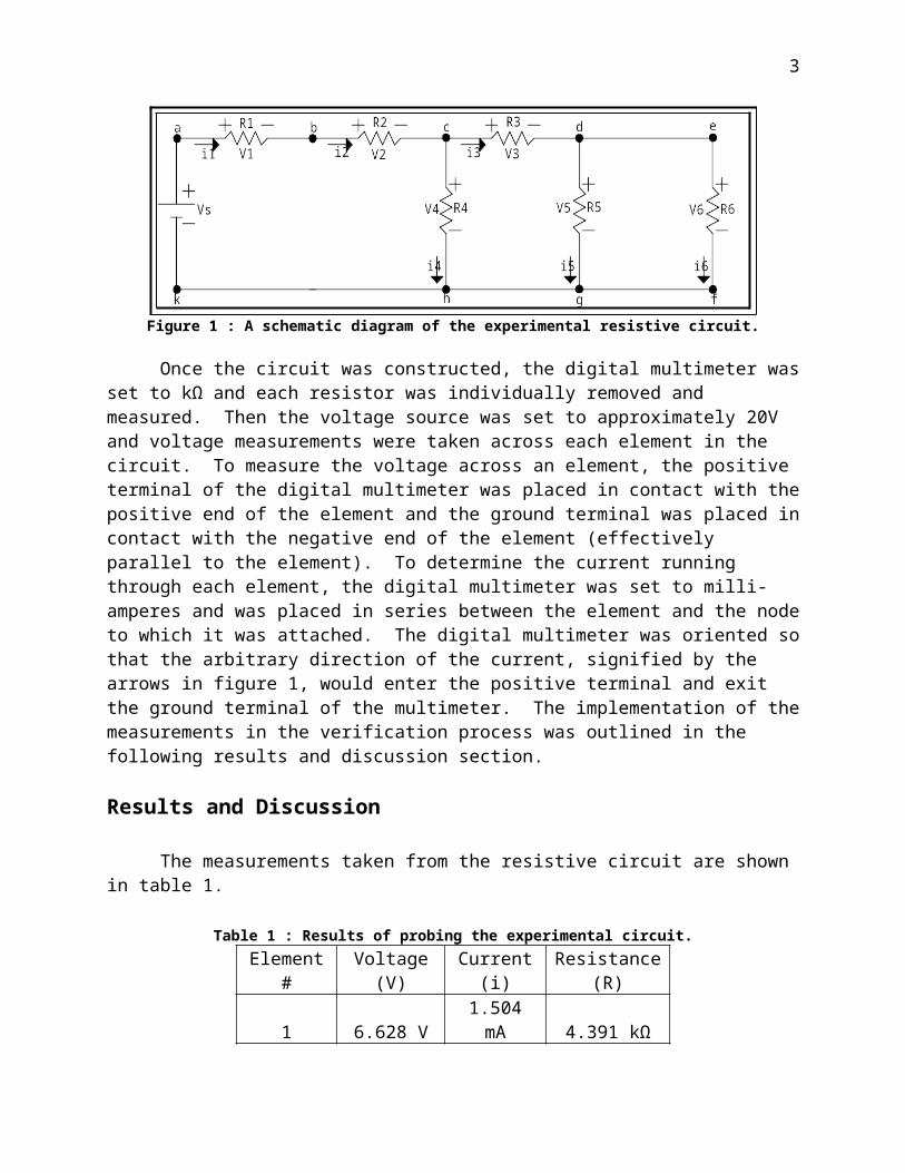
The resistive circuit was constructed by placing the wires and resistors into the breadboard like the schematic shown in figure 1.

Figure 1 : A schematic diagram of the experimental resistive circuit.

Once the circuit was constructed, the digital multimeter was set to kΩ and each resistor was individually removed and measured. Then the voltage source was set to approximately 20V and voltage measurements were taken across each element in the circuit. To measure the voltage across an element, the positive terminal of the digital multimeter was placed in contact with the positive end of the element and the ground terminal was placed in contact with the negative end of the element (effectively parallel to the element). To determine the current running through each element, the digital multimeter was set to milli-amperes and was placed in series between the element and the node to which it was attached. The digital multimeter was oriented so that

3

the arbitrary direction of the current, signified by the arrows in figure 1, would enter the positive terminal and exit the ground terminal of the multimeter. The implementation of the measurements in the verification process was outlined in the following results and discussion section.

Results and Discussion

The measurements taken from the resistive circuit are shown in table 1.

Table 1 : Results of probing the experimental circuit.Element # Voltage (V) Current (i) Resistance (R)

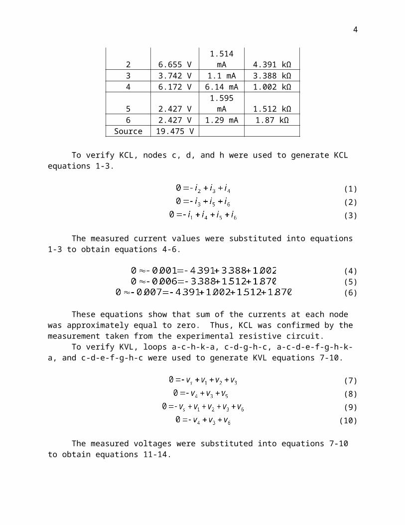
1 6.628 V 1.504 mA 4.391 kΩ2 6.655 V 1.514 mA 4.391 kΩ3 3.742 V 1.1 mA 3.388 kΩ4 6.172 V 6.14 mA 1.002 kΩ5 2.427 V 1.595 mA 1.512 kΩ6 2.427 V 1.29 mA 1.87 kΩ

Source 19.475 V    

To verify KCL, nodes c, d, and h were used to generate KCL equations 1-3.

(1)(2)(3)

The measured current values were substituted into equations 1-3 to obtain equations 4-6.

(4)(5)(6)

These equations show that sum of the currents at each node was approximately equal to zero. Thus, KCL was confirmed by the measurement taken from the experimental resistive circuit.

To verify KVL, loops a-c-h-k-a, c-d-g-h-c, a-c-d-e-f-g-h-k-a, and c-d-e-f-g-h-c were used to generate KVL equations 7-10.

(7) (8)

(9)(10)

The measured voltages were substituted into equations 7-10 to obtain equations 11-14.

4

(11) (12)

(13) (14)

These equations show that sum of the voltages around each loop was approximately equal to zero. Thus, KVL was also confirmed by the measurements taken from the experimental resistive circuit.

To verify Ohm’s law current and resistance terms were substituted into the voltage terms in KVL loop equations a-b-c-h-j-a, c-d-g-h-c, and d-e-f-g-d, to create equations 15-17.

(15)(16)(17)

Equations 1, 2, 15, 16, and 17 were put into matrix form to solve for the current values of each element as shown in equation 18.

(18)

The solution of equation 18 verifies ohm’s law when the measured current values in table 1 are compared to these calculated values.

Conclusion

Through this experiment Ohm’s Law, KVL and KCL were verified by the measurements taken from an experimental resistive circuit. Equations were created by implementing KVL and KCL. The measurements were substituted into the equations to show that they are nearly equal to zero. Ohm’s law was substituted into three of the KVL equations which were then put into matrix form along with two current equations. The matrix was solved to find current values and the comparison of the calculated and measure current for each element verified Ohm’s Law.