e.g.m. petrakisdynamic vision1 dynamic vision copes with –moving or changing objects (size,...

E.G.M. Petrakis Dynamic Vision 1

Dynamic Vision

• Dynamic vision copes with – Moving or changing objects (size, structure, shape)– Changing illumination – Changing viewpoints

• Input: sequence of image frames– Frame: Image at a particular instant of time– Differences between frames: due to motion of camera

or object, illumination changes, changes of objects

• Output: detect changes, compute motion of camera or object, recognize moving objects etc.


• There are four possibilities:– Stationary Camera, Stationary Objects (SCSO)– Stationary Camera, Moving Objects (SCMO)– Moving Camera, Stationary Objects (MCSO)– Moving Camera, Moving Objects (MCMO)

• Different techniques for each case– SCSO is simply static scene analysis: simplest– MCSO most general and complex case– MCSO, MCMO in navigation applications

• Dynamic scene analysis more info can be easier than static scene analysis


• Frame sequence: F(x,y,t)– Intensity of pixel x, y at time t– Assume that t represents the t-th frame– The image is acquired by camera at the origin of

the 3-D coordinate system

• Detect changes in F(x,y,t) between successive frames – At pixel, edge, region level– Aggregate changes to obtain useful info (e.g.,

trajectories)


• Difference Pictures: Compare the pixels of two frames

– Where τ is a user defined threshold– Pixels with value 1 result from motion or

illumination changes– Assumes that the frames are properly registered– Thresholding is important: slow moving objects

may not be detected for a given τ

otherwise

kyxFjyxFifyxDPjk 0

|),,(),,(|1),(


(a), (b): frames from a sequence with change in illumination(c ): their difference thresholded with τ=25

(a), (b): frames from a sequence with moved objects(c ): their difference thresholded with τ=25


• Size filtering: only pixels that belong to a 4 or 8 connected component with intensity larger than τ are retained– Result of size filtering with τ = 10– Removes mainly noisy regions


• Robust change detection: intensity characteristics of regions are compared using a statistical criterion– Super-pixels: nxm non-overlapping rectangles– Local mask: groups of pixels of local pixel area

2*1

)(

0

1),(

2222

2121

otherwise

yxDPjk


(a) Super-pixels(b) Mask of local pixel area

Robust change detection with(a) Super-pixels (super-pixel

Resolution)(b) Pixel masks


• Accumulative difference pictures: analyze changes over a sequence of frames– Compare every frame with a reference frame– Increase a difference term by 1 whenever the

difference is greater than the threshold

– Detects even small or slowly moving objects– Eliminates small misregistration between

frames

),(),(),(

0),(

11

0

yxDPyxADPyxADP

yxADP

kkk


Change detection using accumulative differences(a),(b): first and last frames(c): accumulative difference picture


• Segmentation using motion: find objects in SCMO and MCMO scenes– SCMO: separate moving objects from stationary

background– MCMO: remove the motion due to camera– Correspondence problem: the process of

identifying the same object of feature in two or more frames

– Large number of features put restrictions on the number of possible matches

– Regions, corners, edges …


1. Temporal and Spatial Gradients: Compute

– dF/ds: spatial gradient– dF/dt: temporal gradient– Apply threshold to the product – Responds even to slow moving edges

dt

tyxdF

ds

tyxdFtyxEt

),,(),,(),,(


(a),(b): two frames of a sequence(c): edges detected using spatial-temporal gradients


2. Using difference pictures (stationary camera): difference and accumulative difference pictures find moving areas

)y,x(NDP)y,x(NADP)y,x(NADP

)y,x(PDP)y,x(PADP)y,x(PADP

)y,x(DP)y,x(AADP)y,x(AADP

otherwise

T),y,x(F),y,x(F)y,x(NPDP

otherwise

T),y,x(F),y,x(F)y,x(PDP

otherwise

T|),y,x(F),y,x(F|)y,x(DP

nnn

nnn

nnn

11

11

11

12

12

12

0

211

0

211

0

211


• The area in PADP, NADP is the area covered by the moving object in the reference frame– PADP, NADP continue to increase in value but

the regions stops growing in size– Use a mask of the object to determine whether a

region is growing– Masks can be obtained from AADP when the

object has been completely displaced – In cases of occlusion monitor changes in regions


(a)-(c): frames 1,5,7, containing a moving object(d),(e),(f): PADP, NADP, AADP


• Motion correspondence: to determine the motion of objects establish a correspondence between features in two frames– Correspondence problem: pair a point pi=(xi,yi) in

the first image with a point pj=(xj,yj) in the second image

– Disparity: dij=(xi - xj,yi - yj)

– Compute disparity using relaxation labeling– Questions: how are points selected for matching?

how are the correct matches chosen? what constraints?


• Three properties guide matching: – Discreteness: minimize expensive searching

(detect points at which intensity values are varying quickly in at least one direction)

– Similarity: match similar features (e.g., corners, edges, etc.)

– Consistency: match nearby points (a point cannot move everywhere)

correspondence problem as bipartite graph matching between two frames A, B:remove all but one connection for each point


• Disparity computation using Relaxation Labeling: – Identify the features to be matched – E.g., corners or (generally) points i, j

– Let Pij0 be the initial probability

– Disparity: dij=(xi - xj,yi - yj) < Dmax

2

||21

0

),,(),,(

1

1

xdjjjjiiiiij

ijij

x

tdyydxxFtdyydxxFw

wP

points cannot move everywhere

high probabilities for pointsin dx with similar motion

neighborhood


• Update Pij at every iteration:

• For every point i, the algorithm computes

{i, (dxij,Pij)0, (dxij,Pij)1,…. (dxij,Pij)n}– n: n-th iteration or frame

• Use correspondences with high Pij

• Use these for the next two frames etc.

xd lk

nkl

nij

dxij

nij

ijnijn

ij

pq

BqAP

BqAPP

,

11

1

1

)(

)(


n0 1 3 4

Disparities after 3 iterations

From Ballardand Brown, 94


disparities after Applying a relaxation

labeling algorithm


• Image flow: velocity field in the image due to motion of the observer, objects or both– Velocity vector of each pixel– Image flow is computed at each pixel – SCMO: most pixels will have zero velocity

• Methods: pixel and feature based methods compute image flow for all pixels or for specific features (e.g., corners)– Relaxation labeling methods– Gradient Based methods


• Gradient Based Methods: exploit the relationship between spatial and temporal gradients of intensity– Assumption: continuous and smooth changes of

intensity in consecutive frames

uFt

F

uy

Fu

x

F

dt

dy

y

F

dt

dx

x

F

t

F

termsorderhighdtt

Fdy

y

Fdx

x

FtyxF

dttdyydxxFtyxF

yx

),,(

),,(),,( Taylor expansion


• Better estimation: the error term is not zero– It has to be minimum: Apply Lagrange

multipliers method

– fx, fy,ft: derivatives of F with regard to x,y and t

– The derivative of F2 with regard to x,y is zero– From Ballard and Brown 1984 – The computation can be unreliable at motion

boundaries (e.g., occluded boundaries)

})(){()fufu(ft)y,(x,F 222222tyyxx

2yx uu


D

Pfuu

D

Pfuu

ffD

fufufP

uuu

uuu

ffuuffuf

ffuuffuf

yaverageyy

xaveragexx

yx

taverageyyaveragexx

averageyyy

averagexxx

yaverageyxyxyy

txaveragexyyxxx

222

22

22

222

222

)(

)(

Turn this into an iterative method for solving ux,uy


• Optical flow computation for two consecutive frames (Horn & Schunck 1980)– k=0

– Initialize all uxk=uy

k=0

– Repeat until some error criterion in satisfied

D

Pfuu

D

Pfuu

yaverageyy

xaveragexx


• Multi-frame optical flow: compute optical flow for two frames and use this to initialize optical flow for the next frame etc.– k=0

– Initialize all ux,uy (apply the previous algorithm)

– Repeat until some error criterion in satisfied

D

Pftyxutyxu

D

Pftyxutyxu

yaverageyy

xaveragexx

)1,,(),,(

)1,,(),,(


(a),(b),(c): three frames from a rotating sphere(d): optical flow after 32 frames

from Ballard andBrown’84


• Information in optical flow: assuming high quality computation of optical flow – Areas of smooth velocity single surfaces– Areas with large gradients occlusion and

boundaries– The translation component of motion is directed

toward the Focus Of Expansion (FOE): intersection of the directions of optical flow as seen by a moving observer

– Surface structure can be derived from the derivatives of the translation component

– Angular velocity can be determined from the rotational component


• The velocity vectors of the stationary components of a scene as seen by a translating observer meet at the Focus Of Expansion (FOE)


• Tracking: a feature or an object must be tracked over a sequence of frames– Easy to solve for single entities – For many entities moving independently

requires constraints– Path coherence: the motion of an object in a

frame sequence doesn't change abruptly between frames (assumes high sampling rate)

• The location of a point will be relatively unchanged • The scalar velocity of a point will be relatively

unchanged• The direction of motion will be relatively unchanged


• Deviation function for path coherence:– A trajectory of a point i: Ti=<Pi

1,Pi2,…,Pi

n>

– Pik: point i at k-th frame

– In vector form: Xi=<Xi1,Xi

2,…,Xin>

– Deviation of the point in the k-th frame: di

k=φ(Xik-1Xik,XikXik+1)

– Deviation for the complete trajectory: – For m points (trajectories) in a sequence of n

frames the total deviation is– Minimize D to find the correct trajectories

ki

1

2i dD

n

k

m

i

n

k

kim dTTTD

1

1

221 ),...,,(


• The trajectories of 2 points: The points in the 1st, 2nd and 3rd frame are labeled by squares, triangles and rhombus respectively• The change in the direction and velocity must be smooth


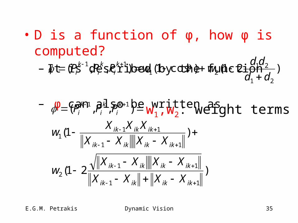
• D is a function of φ, how φ is computed? – It is described by the function

– φ can also be written as

)21()cos1(),,(21

2121

11

dd

ddwwPPP k

iki

ki

)21(

)1(

),,(

11

112

11

111

11

ikikikik

ikikikik

ikikikik

ikikik

ki

ki

ki

XXXX

XXXXw

XXXX

XXXw

PPP w1,w2: weight terms


• Direction coherence: the first term– Dot product of displacement vectors

• Speed coherence: the second term– Geometric/arithmetic mean of magnitude

• Limitations: same number of features in every frame– Objects may disappear, appear or occlude– Changes of geometry, illumination– Lead to false correspondences– Force the trajectories to satisfy certain local

constraints

e.g.m. petrakisdynamic vision1 dynamic vision copes with –moving or changing objects (size,...

Documents