EFFICIENT ESTIMATION OF THE SEMIPARAMETRIC SPATIAL AUTOREGRESSIVE MODEL

Peter Robinson

THE INSTITUTE FOR FISCAL STUDIESDEPARTMENT OF ECONOMICS, UCL

cemmap working paper CWP08/06

E¢ cient Estimation of the SemiparametricSpatial Autoregressive Model

P.M. Robinson�

Department of Economics, London School of Economics,Houghton Street, London WC2A 2AE, UK

February 27, 2006

Abstract

E¢ cient semiparametric and parametric estimates are developed for aspatial autoregressive model, containing nonstochastic explanatory vari-ables and innovations suspected to be non-normal. The main stress is onthe case of distribution of unknown, nonparametric, form, where seriesnonparametric estimates of the score function are employed in adaptiveestimates of parameters of interest. These estimates are as e¢ cient asones based on a correct form, in particular they are more e¢ cient thanpseudo-Gaussian maximum likelihood estimates at non-Gaussian distri-butions. Two di¤erent adaptive estimates are considered. One entails astringent condition on the spatial weight matrix, and is suitable only whenobservations have substantially many "neighbours". The other adaptiveestimate relaxes this requirement, at the expense of alternative conditionsand possible computational expense. A Monte Carlo study of �nite sampleperformance is included.

JEL Classi�cations: C13; C14; C21Keywords: Spatial autoregression; E¢ cient estimation; Adaptive esti-

mation; Simultaneity bias.

�Corresponding author: Tel. +44-20-7955-7516; fax: +44-20-7955-6592.E-mail address: p.m.robinson@lse.ac.uk.

1

1 Introduction

Spatial autoregressive models have proved a popular basis for statistical infer-ence on spatial econometric data. Much of the spatial statistics literature hasfocussed on data recorded on a lattice, that is, it is regularly-spaced in two ormore dimensions. This is an unlikely framework in economics, at best an approx-imation. Data recorded over geographical space are apt to be very irregularlyspaced, such as at cities or towns, or aggregated across possibly contiguous re-gions, such as provinces or countries. A recent review of spatial econometricsis Arbia (2006). A statistical model that adequately describes dependence as afunction of geographic distance is apt to be complicated, especially in the secondkind of situation, and derivations of rules of large sample statistical inferenceunder plausible conditions di¢ cult; even for time series data, where there is asingle dimension, inference in irregularly-spaced settings is not very well devel-oped. On the other hand, cross-sectional correlation has been measured as afunction of "economic distance", not necessarily in a geographic setting. Spatialautoregressive models are applicable in all these circumstances.We wish to model an n�1 vector of observations y = (y1; :::; yn)T , on a scalar

variate yi, T indicating transposition. We have an n � k matrix of constantsX = (x1; :::; xn)

T , xi being a k � 1 vector, where k � 1. Let " = ("1; :::; "n)T

be an n� 1 vector of unobservable random variables, that are independent andidentically distributed (iid) with zero mean and unit variance. Let ln be then� 1 vector (1; :::; 1)T . Finally, let W be a given n�n "weight" matrix, havingzero diagonal elements and being row-normalized such that elements of eachrow sum to 1, so

Wln = ln: (1.1)

We assume that, for some scalars �0, �0 and �0, and some k � 1 vector �0,

y = �0ln + �0Wy +X�0 + �0": (1.2)

Here, �0 and �0 > 0 are unknown nuisance parameters, representing interceptand scale respectively: they can be estimated, but our focus is on the estimationof �0 = (�0; �

T0 )T , where �0 2 [0; 1) and �0 is non-null. It is taken for granted

that there are no restrictions linking �0; �0 and �0. It is assumed that thematrix (ln; X) has full column rank for su¢ ciently large n, and because k � 1there must be at least one non-intercept regressor.The weight matrix W has to be chosen by the practitioner. In view of

the row-normalization, we can de�ne it in terms of an underlying non-negativeinverse "distance" measure dij such that W has (i; j)-th element

wij =dijnPh=1

dih

: (1.3)

However, the "distance" terminology is not taken to imply thatW is necessarilya symmetric matrix.

2

In general, only large-sample statistical inference can be justi�ed. Here,though we have mostly suppressed reference to the data size n for the sake ofa concise notation, the row-normalization of W implies that as n!1, y mustbe treated like a triangular array. In recent years considerable progress hasbeen made in the econometric literature on developing asymptotic properties ofvarious estimates for (1.2).Ordinary least squares (OLS) comes �rst to mind. The OLS estimate of

�0 in (1.2) (with �0 treated as unknown) is generally inconsistent, because, foreach i, the i-th element of Wy is correlated with "i. This situation contrastswith the corresponding classical dynamic time series model in which the laggeddependent variable is uncorrelated with the disturbance. It mirrors the oneidenti�ed by Whittle (1954), in case of multilateral autoregressive models ona lattice. He pointed out that the problem is corrected by using Gaussianmaximum likelihood (ML) estimation: the determinant term in this, whichOLS neglects, has non-negligible e¤ect.This is the case also in (1.2), and Lee (2004) has established desirable asymp-

totic properties of Gaussian ML here, namely n12 -consistency and asymptotic

normality and e¢ ciency. An alternative, if generally sub-optimal solution, is in-strumental variables, and this has been justi�ed by Kelejian and Prucha (1998,1999), Lee (2003), Kelejian, Prucha and Yuzefovich (2003).On the other hand, returning to OLS, Lee (2002) noticed that this can still

be consistent, and even n12 -consistent and asymptotically normal and e¢ cient

under suitable conditions on W . In particular, he showed that consistency ispossible if the dij in (1.3) are uniformly bounded and the

Pnj=1 dij tend to

in�nity with n, and n12 -consistent if the latter sums tend to in�nity faster than

n12 .This can be simply illustrated in terms of a W employed in an empirical

example of Case (1992), and stressed by Lee (2002). Data are recorded acrossp districts, in each of which are q farmers. Independence between farmers indi¤erent districts is assumed, and neighbours at each farm within a district aregiven equal weight. Due to (1.1) we have

W = Ip (q � 1)�1�lql

Tq � Iq

�: (1.4)

In this setting, OLS is consistent if

q !1; as n!1; (1.5)

and n12 -consistent if

q=p!1 as n!1: (1.6)

The procedure considered by Lee (2004), on the other hand, was actuallyinterpreted not just as ML under Gaussianity, but also pseudo-ML under depar-tures from Gaussianity, as is the case in many other settings. However, thoughn12 -consistency and asymptotic normality is relevant in the latter circumstances,asymptotic e¢ ciency is not. When data-sets are not very large, precision is im-portant, and since there is often reason not to take Gaussianity seriously, it isdesirable to develop estimates which are e¢ cient in non-Gaussian populations.

3

As is typically the case in time series models, building a non-Gaussian like-lihood is most easily approached by introducing a non-normal distribution forthe iid "i in (1.2), for example a Student-t distribution. Such a distributionmay also involve unknown nuisance parameters, to be estimated alongside theoriginal ones. We present limit distributional results for one-step Newton ap-proximations to ML estimates in this case. However, there is rarely a strongreason for picking a particular parametric form for the underlying innovationdensity, and if this is mis-speci�ed not only would the estimates not be asymp-totically e¢ cient (or necessarily more e¢ cient than the Gaussian pseudo-MLestimates of Lee (2004)), but in some cases they may actually be inconsistent.As in other statistical problems, these drawbacks, as well as possible computa-tional complications, do much to explain the popularity of Gaussian pseudo-MLprocedures, and approximations to them.On the other hand, the ability to "adapt" to distribution of unknown form is

well-established in a number of other statistical and econometric models. Herethe density f of "i in (1.2) is regarded as a nonparametric function, so that (1.2)is a semiparametric model, and f is estimated by smoothing. By a suitableimplementation, it can then be possible to obtain estimates of the parametersof the model that are n

12 -consistent and normal, and asymptotically as e¢ cient

as ones based on a correctly parameterized f . This was demonstrated by Stone(1975), for the simple location model with iid data, and then by Bickel (1982),Newey (1988) for regression models with iid errors, and by other authors invarious other models. The main focus of the present paper is to develop suchprocedures for e¢ ciently estimating the vector �0 in (1.2). The ability to adaptin (1.2) is not guaranteed. Our �rst result requires similar conditions on Wto those that Lee (2002) imposed in justifying the n

12 -consistency of OLS (i.e.

(1.6) in case (1.4)). Our second result employs a bias-reduced estimate that, incase (1.4), requires only (1.5), though either W has also to be symmetric (as isthe case in (1.4)) or "i has to be symmetrically distributed.Our e¢ cient estimates of �0 are described in the following section. Regu-

larity conditions and theorem statements are presented in Section 3. Section 4consists of a Monte Carlo study of �nite sample behaviour. Proofs are left toan appendix.

2 E¢ cient Estimates

It is possible to write down an objective function that is a form of likelihood,employing a smoothed nonparametric estimate of the density f of the "i. How-ever, not only is this liable to be computationally challenging to optimize, butderivation of asymptotic properties would be a lengthy business since, as is com-mon in problems involving implicitly-de�ned extremum estimation, the proof ofn12 -consistency and asymptotic normality has to be preceded by a consistencyproof. The latter can be by-passed by the familiar routine of taking one Newton-type iterative step, based on the aforementioned "likelihood", from an initial

4

n12 -consistent estimate. This strategy is followed virtually uniformly in theadaptive estimation literature, and we follow it here.It leads to the need to nonparametrically estimate not f(s), but the score

function

(s) = �f0(s)

f(s); (2.1)

where throughout the paper the prime denotes di¤erentiation. The bulk of workon adaptive estimation uses kernel estimates of f and f 0. Kernel estimation isvery familiar in econometrics, and can have important advantages. However,separate estimation of f and f 0 is necessary, and the resulting estimate of issomewhat cumbersome.More seriously, since f is liable to become small, use of an estimate in the de-

nominator of (2.1) is liable to cause instability. It also causes technical di¢ culty,and typically some form of trimming is introduced. This requires introductionof a user-chosen trimming number, itself a disincentive to the practitioner. Inaddition, kernel-based adaptive estimates have, for technical reasons, featuredsample-splitting (use of one part of the sample in the nonparametric estimation,and the other for the �nal parametric estimation) which is wasteful of data andintroduces a further ambiguity, as well as the arti�cial device of discretizing theinitial parameter estimate.These drawbacks are overcome by employing a series estimate of , as pro-

posed by Beran (1976) in the context of estimation of the coe¢ cients of a timeseries autoregressive model. Let �`(s), ` = 1; 2; :::, be a sequence of smoothfunctions. For some user-chosen integer L � 1, de�ne the vectors

�(L)(s) = (�1(s); :::; �L(s))T; ��

(L)(s) = �(L)(s)� E

n�(L)("i)

o: (2.2)

Consider for (s) �rst the parametric form

(s) = ��(L)(s)Ta(L); (2.3)

where a(L) = (a1; :::; aL)T is a vector with unknown elements. The mean-

correction in (2.2) imposes the restriction E f ("i)g = 0. Under mild conditionson f , integration-by-parts allows a(L) to be identi�ed by

a(L) =hEn��(L)("i)��

(L)("i)

Toi�1

En��(L)0("i)o: (2.4)

Given a vector of observable proxies ~" = (~"1; :::;~"n)T , we approximate a(L) by

~a(L)(~"), where, for a generic vector q = (q1; :::; qn)T;

~a(L)(q) =W (L)(q)�1w(L)(q); (2.5)

with

W (L)(q) =1

n

nPi=1

�(L)(qi)�(L)(qi)

T ; (2.6)

w(L)(q) =1

n

nPi=1

�(L)0(qi); (2.7)

5

and

�(L)(qi) = �(L)(qi)�1

n

nPj=1

�(L)(qj): (2.8)

Then de�ning

(L)�qi; ~a

(L)(q)�= �(L)(qi)

T ~a(L)(q); (2.9)

~ il = (L)�~"i; ~a

(L)(~")�is a proxy for ("i), and is inserted in the Newton step

for estimating the unknown parameters.However, Beran�s (1976) asymptotic theory assumed that, for the chosen L,

(2.3) correctly speci�es (s). This amounts almost to a parametric assumptionon f : indeed, if we took L = 1 and �1(s) = s, (s) given by (2.3) is just thescore function for the standard normal distribution. Newey (1988) considerablydeveloped the theory by allowing L to go to in�nity slowly with n, so that theright hand side of (2.3) is an approximation to (an in�nite series representationof) (s), and thence (in regression with independent cross-sectional observa-tions) establishing analogous adaptivity results to those, say, that Bickel (1982)had, using kernel estimation of . Robinson (2005) developed Newey�s (1988)asymptotic theory further, in the context of stationary and nonstationary frac-tional time series models. In the asymptotic theory, L can be regarded as asmoothing number analogous to that used in a kernel approach, but no otheruser-chosen numbers or arbitrary constructions are required in the series ap-proach, where indeed some regularity conditions are a little weaker than thosein the kernel-based literature.We follow the series estimation approach here, and for ease of reference

mainly follow the notation of Robinson (2005). To provide further details forthe adaptive estimation of our �0, consider the n� 1 vector

e(�) = (e1(�); :::; en(�))T= (I � �W )y �X�; (2.10)

for � =��; �T

�T, and any scalar � and k � 1 vector �. From (1.2)

�0" = e(�0)� E fe(�0)g : (2.11)

Accordingly, given an initial estimate ~� of �0, consider as a proxy for the vector�0" the vector E(~�), where

E(�) = e(�)� ln1

n

nPi=1

ei(�): (2.12)

We can estimate �20 by ~�2 = ~�2(~�); where

~�2(�) =1

nE(�)TE(�): (2.13)

Thus our proxy ~" for " is given by

~" = E(~�)=~�: (2.14)

6

We �nd it convenient to write

~ iL =~ iL(

~�; ~�); (2.15)

where~ iL(�; �) = �

(L) (Ei(�)=�)T~a(L) (E(�)=�) : (2.16)

Now introduce the n� (k + 1) matrix of derivatives

e0 =

�@e(�)

@�;@e(�)

@�T

�T; (2.17)

in which

@e(�)

@�= �Wy; (2.18)

@e(�)

@�= �XT ; (2.19)

for all �: With e0i denoting the i-th column of e0 write

E0i = e0i �1

n

nPj=1

e0j : (2.20)

Now de�ne

R =nPi=1

E0iE0Ti ; (2.21)

and

rL(�; �) =nPi=1

~ iL(�; �)E0i; (2.22)

and let~

IL(�; �) =1

n

nPi=1

~ 2

iL(�; �); (2.23)

so~

IL(~�; ~�) estimates the information measure

I = E ("i)2: (2.24)

Our �rst adaptive estimate of �0 is

�A = ~� ��~

IL(~�; ~�)R��1

rL(~�; ~�): (2.25)

(There is a typographical error in the corresponding formula (2.2) of Robinson(2005): " + " should be "� ":) De�ne

sL(�; �) = rL(�; �) +

�tr�W (In � �W )�1

0

�; (2.26)

7

so sL and rL di¤er only in their �rst element. Our second adaptive estimate of�0 is

�B = � ��~

IL(~�; ~�)R��1

sL(~�; ~�): (2.27)

There are some practical issues outstanding. One is the choice of the func-tions �`(s). As in Newey (1988), Robinson (2005), we restrict to "polynomial"forms

�`(s) = �(s)`; (2.28)

for some chosen function �(s). For example,

�(s) = s; (2.29)

�(s) =s

(1 + s2)12

; (2.30)

where the boundedness in (2.30) can help to reduce other technical assumptions.Next, the choice of L is discussed in some detail by Robinson (2005); asymptotictheory provides little guidance here, indeed it delivers an upper bound on therate at which L can increase with n, but no lower bound. Since the upper boundis only logarithmic in n, it seems that values of L should be used that are farsmaller than n. Discussion of the choice of ~� is postponed to the followingsection.For completeness, we also consider the fully parametric case, where f(s; �0)

is a prescribed parametric form for f(s), with �0 an unknown m� 1 vector, onthe basis of which de�ne b� = argmin

T

Pi

log f(Ei(e�)=e�; �) for a subset T of Rm,and, with (s; �) = (@=@s)f(s; �)=f(s; �)

~

IL(�; �; �) = n�1Pi

(Ei(�)=�; �)2; (2.31)

rL(�; �; �) =Pi

(Ei(�)=�; �)E0i(�): (2.32)

De�ne also

sL(�; �; �) = rL(�; �; �) +

�tr�W (In � �W )�1

0

�: (2.33)

Our two parametric estimates are

�C = ~� ��~

IL(~�; ~�;b�)R��1 rL(~�; ~�;b�); (2.34)

�D = ~� ��~

IL(~�; ~�;b�)R��1 sL(~�; ~�;b�); (2.35)

the second being a "bias-corrected" version of the �rst.

8

3 Asymptotic Normality and E¢ ciency

We introduce �rst the following regularity conditions

Assumption 1: For all su¢ ciently large n, the weight matrix W has non-negative elements that are uniformly of order O(1=hn), where

hn=n12 !1; as n!1; (3.1)

and has zero diagonal, satis�es (1.1), and is such that the elements of lTnW andlTnS

�1 are uniformly bounded, where S = In � �0W .

Assumption 2: The elements of the xi are uniformly bounded constants, andthe matrix

= limn!1

1

n

�(GX�0)

T

XT

�[GX�0; X] (3.2)

exists and is positive de�nite, where G =WS�1.

Assumption 3: The "i are iid with zero mean and unit variance, and proba-bility density function f(s) that is di¤erentiable, and

0 < I <1: (3.3)

Assumption 4: �`(s) satis�es (2.28), where �(s) is strictly increasing andthrice di¤erentiable and is such that, for some � � 0, K <1,

j�(s)j � 1 + jsjK (3.4)���0(s)��+ ���00(s)��+ ���000(s)�� � C�1 + j�(s)jK

�; (3.5)

where C is throughout a generic positive constant.Denote by � = 1+2

12 l 2:414 and ' = (1+ j�(s1)j = f�(s2)� �(s1)g, [s1; s2]

being an interval on which f(s) is bounded away from zero.

Assumption 5:L!1; as n!1; (3.6)

and either(i) � = 0, E"4i <1, and

limn!1

�log n

L

�> 8 flog � +max(log'; 0)g ' 7:05 + 8max (log'; 0) ; (3.7)

or (ii) � > 0 for some ! > 0 the moment generating function E�etj"ij

!�exists

for some t > 0, and

lim infn!1

�log n

L logL

�> max

�8K

!;4�(! + 1)

!

�; (3.8)

9

or (iii) � > 0, "i is almost surely bounded, and

lim infn!1

�log n

L logL

�> 4�: (3.9)

Assumption 6: As n!1

~� � �0 = Op(n� 12 ); ~�2 � �20 = Op(n

� 12 ): (3.10)

The proof of the following theorem is left to the Appendix.

Theorem A Let (1.2) hold with �0 2 [0; 1), and let Assumptions 1-6 hold.Then as n!1

n12

��A � �0

�!d N

�0;�20I

�1�; (3.11)

where the limit variance matrix is consistently estimated by�~�2=

~

IL(~�; ~�)�nR�1.

Remark 1 For the Gaussian pseudo-ML estimate, Lee (2004) �nds the limitingvariance matrix to be �2�1. Since I � 1, �A achieves an e¢ ciency improve-ment over this when "i is non-Gaussian.

Remark 2 Various initial estimates that satisfy Assumption 1 are availablein the literature. This is the case under (3.1) if ~� is the OLS estimate of �0(see Lee, 2002). Other possibilities are the Gaussian pseudo-ML estimate, andvarious IV estimates.

Remark 3 In view of Assumption 2, �0 cannot be the null vector (cf. Lee(2004)), so Theorem A cannot be used to test �0 = 0, though it can be usedto test exclusion of a proper subset of the elements of xi. It can also be usedto test the hypothesis of no spatial dependence, �0 = 0, and in this case thelimit distribution in the Theorem is true even if (3.1) does not hold, indeed hncan be regarded as �xed with respect to n, and so designs with only very few"neighbours" are covered. For non-Gaussian data, the tests provided by theTheorem are in general expected to be locally more powerful than ones basedon existing estimates.

Remark 4 Assumption 1 is discussed by Lee (2002). In case W is given by(1.4), hn � q, so condition (3.1) is equivalent to (1.6), and the rest of Assumption1 is satis�ed.

Remark 5 Assumptions 3-5 are essentially taken from Robinson (2005), wherethey are discussed. The main implications are that if we choose bounded �(s)then a fourth moment condition on "i su¢ ces, with a relatively mild upperbound restriction on the rate of increase of L (see (i)). For unbounded �(s), wehave a choice between moment generating function (ii) and boundedness (iii)requirements on "i, where the condition on L is weaker in the latter case, butstill stronger than that of (i) of Assumption 5.

10

Remark 6 It would be possible to obtain analogous results for a non-linearregression extension of (1.2), in which the elements of X�0 are replaced by thenonlinear-in-�0 functions g(xi;�0), i = 1; :::; n, where g is a smooth function ofknown form. With respect to the initial estimate ~� it would seem that non-linearleast squares can be shown to satisfy Assumption 6 under (3.1), by extendingthe arguments of Lee (2002).Remark 7 In practice further iteration of (2.25) may be desirable. Thiswould not change the limit distribution, but can improve higher-order e¢ ciency(Robinson, 1988).By far the most potentially restrictive of the conditions underlying Theorem

1 is (3.1) of Assumption 1. It is never really possible to gauge the relevance ofan asymptotic condition such as this to a given, �nite, data set. However, if, inthe simple case where W is given by (1.4), q is small relative to p, one expectsthat �A may be seriously biased, and the normal approximation poor; the samewill be true of OLS.Results of Lee (2004) on the Gaussian pseudo-MLE hint at how it may be

possible to relax (3.1). To best see this we temporarily modify the model (1.2)to

y = �0Wy + Z 0 + �0": (3.12)

If an intercept is allowed, as in (1.2), then ln is a column of Z, Z = (ln; X),and 0 = (�0; �

T0 )T . But it is also possible that no intercept is allowed, unlike

in (1.2), in which case Z = X and 0 = �0 (and �0 = 0). The form (3.12) isthe most usual in the literature. Lee (2004) shows the Gaussian pseudo-MLE

��=���; �T ; ��2

�Tof �0 =

��0;

T0 ; �

20

�Tis n

12 -consistent and asymptotically

normal, under mild conditions that do not even require that hn diverge (i.e. in(1.4), q can remain �xed). However, even under Gaussianity, �

�and ��2 are

independent in the limit distribution if hn does not diverge, suggesting thatadaptive estimation of �0; 0 is not possible in this scenario. Lee (2004) �nds,however, that the limit covariance matrix of �

�simpli�es when

hn !1; as n!1; (3.13)

(i.e. (1.5) under (1.4)). His formulae indicate that���; �T

�Tand ��2 will then

be asymptotically independent if E�"3i�lTnGZ 0=n ! 0, E

�"3i�lTn =n ! 0, as

n!1. This is true if "i is normally distributed, and somewhat more generally,e.g. if "i is symmetrically distributed. Reverting now to our model (1.2) and

with (��; �

�T; ��2) denoting the Gaussian pseudo-MLE of

��0; �

T0 ; �

20

�, analo-

gously���; �

�T�and ��2 are asymptotically independent if

E("3i )lTnGHX�0=n! 0; E("3i )l

TnHX=n! 0; as n!1; (3.14)

where H = In � lnlTn =n. The latter limit always holds (since l

TnH = 0), indeed

the left hand side is the null vector for all n: The �rst limit holds if W is

11

symmetric (because (1.1) then implies lTnW = lTn ), and again the left hand sideis zero for all n. (Such symmetry obtains in (1.4).) Thus if we focus on �0 andslope parameters only, their estimates are independent of ��2 more generallythan Lee (2004) claims, to enhance further the value of his results.These observations suggest that if we start from a full, but possibly non-

Gaussian likelihood, in the spirit of Whittle (1954), so that it contains a Jaco-bian factor det

12 fIn � �Wg, we will both achieve su¢ cient bias-correction to

enable relaxation of (3.1) to (3.13), and the information matrix block-diagonalitynecessary for adaptivity, so long as either W is symmetric or "i is symmetri-cally distributed (the moments E("3i ) in the above discussion are replaced byE�"i ("i)

2�.

The proof of the following theorem is omitted, due to the preceding dis-cussion, and the fact that our proof of Theorem A focusses on how the biasproblem is resolved by (3.1), and not only is this aspect now unnecessary, butthe remainder of the proof details are partly covered by some given in the proofof Theorem A, while others are relatively straightforward.

Theorem B Let (1.2) hold with �0 2 [0; 1), and let Assumptions 1-6 hold with(3.1) relaxed to (3.13), and let either W be symmetric or "i be symmetricallydistributed. Then as n!1;

n12

�b�B � s�!d N

�0;�20I

�1�; (3.15)

where the limit variance matrix is consistently estimated by�~�2=

~

IL(~�; ~�)�nR�1:

Remark 8 In general �B can be expensive to compute because the secondcomponent of sL(�; �) involves the inverse of an n�n matrix. However, in somespecial cases it is very simple, e.g. in case W is given by (1.4), we have

tr�W (In � �W )�1

=

n�

(q � 1 + �)(1� �) : (3.16)

Remark 9 We cannot use OLS for ~�, ~�2 if (3.1) does not hold. We can,however, use an IV estimate, such as those of Kelejian and Prucha (1998, 1999),Lee (2003), or the Gaussian pseudo-MLE of Lee (2004).

Remark 10 As in other models, under symmetry of "i it is also possible toadapt with respect to the estimation of �0 in (1.2).

With respect to �C and �D we introduce the following additional assump-tions.

Assumption A7 T is compact and � is an interior point of T .

Assumption A8 For all � 2 T � f�0g, f(s; �) 6= f(s; �0) on a set of positivemeasure.

12

Assumption A9 In a neighbourhood N of �0, log f(s; �) is thrice continuouslydi¤erentiable in � for all s andZ 1

�1

�supN

���f (k)(s; �)���+ supN

���f (k;`)(s; �)���+ supN

���f (k;`;m)(s; �)���� ds <1; (3.17)where f (k), f (k;`), f (k;`;m) represent partial derivatives of f with respect to thek-th, the k-th and `-th, and the k-th, `-th and m-th elements of � , respectively.

Assumption A10 = E�(@=@�) log f("i; �0)(@=@�

T ) log f("i; �0)�is positive

de�nite.

Theorem C Let (1.2) hold with �0 2 [0; 1); and let Assumptions 1-3 and6-10 hold. Then as n ! 1, n 1

2 (�C � �0)and n12 (b� � �0) converge to indepen-

dent N(0; (�20=I)�1), and N(0;�1) vectors respectively, where the limiting

covariance matrices are consistently estimated by�~�2=

~

IL(~�; ~�;b�)�nR�1 and�n�1

nPt=1

h(@=@�) log f

�Ei(~�)=~�;b��i h(@=@�T ) log f �Ei(~�)=~�2;b��i��1 ;

(3.18)respectively.

Theorem D Let (1.2) hold with �0 2 [0; 1); and let Assumptions 1-3 and 6-10 hold with (3.1) relaxed to (3.13), and let either W be symmet-ric or "i be symmetrically distributed. Then as n ! 1, n 1

2 (�D � �0)andn12 (b� � �0) converge to independent N(0; (�20=I)�1), and N(0;�1) vectorsrespectively, where the limiting covariance matrices are consistently estimated

by�~�2=

~

IL(~�; ~�;b�)�nR�1 and (3.18) respectively.The proofs would require �rst an initial consistency proof for the implicitly-

de�ned extremum estimate b� , and are omitted because they combine elementsof the proof of Theorem A with relatively standard arguments.Remark 11 The Gaussian MLE can in general be expensive to compute due tothe determinant factor, as discussed by Kelejian and Prucha (1999). However,the limit distribution of this estimate is the same as that of �C and �D whenthese are based on f(s; �) = (2�)�1=2 exp(�s2=2); (s; �) = s: Indeed such �Drepresents a Newton step to the Gaussian MLE.

13

4 Finite Sample Performance

The behaviour of our adaptive estimates in �nite sample sizes was examinedin a small Monte Carlo study. The spatial weight matrix W given by (1.4)was employed, with three di¤erent choices of (p; q): (8,12), (11,18), (14,28).These correspond to n = 96, 198 and 392, and are intended to represent a slowapproach to the asymptotic behaviour of (3.1). For each n, scalar explanatoryvariables x1; :::; xn were generated as iid uniform (0; 1) observations, and thenkept �xed throughout the study, to conform to the non-stochastic aspect ofAssumption 2. The "i were generated from each of the following 5 distributions.

(a) Normal, "i � N(0; 1);

(b) Bimodal Mixture normal, "i = u=p10 where pdf(u) = :5p

2�exp

�� (u�3)2

2

�+

:5p2�exp

�� (u+3)2

2

�;

(c) Unimodal Mixture normal, "i = u=p2:2, where pdf(u) = :05p

50�exp

��u2

50

�+

:95p2�exp

��u2

2

�;

(d) Laplace, f(s) = exp�� jsj

p2�p2;

(e) Student t5; "i = up3=5, where u � t5:

These are fairly standard choices in Monte Carlo studies of adaptive estimates.All of them are scaled to have variance 1, as in Assumption 3. Case (a) has�nite moments of degree 4 only.On each of 1000 replications, y was generated from (1.2) with �0 = 0, 0 = 1,

�0 = 1, and with two di¤erent �0 values, 0.4 and 0.8, for each of the 3 n valuesand 5 "i distributions. Both �A and �B were computed in each case, for bothchoices (2.29) and (2.30) of �(s) (respectively denoted "1" and "2" in the tablesbelow), and for L = 1; 2; 4. We took ~� to be OLS.Lee (2004) featured the design (1.4) in his Monte Carlo study of the Gaussian

MLE. The two experiments are not closely comparable. He employed a widerrange of n and xi, while restricting to Gaussian "i and a single �0 (0:5), andwith no comparison with other estimates. Our study looks at relative e¢ ciencyover a range of distributions, our examination of two values of �0 turns out tothrow light on the bias issue, and we explore aspects of implementation whichdo not arise for his estimate. Nevertheless. we shall have occasion to refer tohis results, and make some remarks about computational issues prompted byboth studies.Monte Carlo bias, variance and mean squared error (MSE) were computed

in each of the 2 � 2 � 2 � 3 � 3 � 5 = 360 cases. In view of the potentialimpact of bias, Tables 1 and 2 report Monte Carlo bias of both elements, e�; e�;of the initial estimate, OLS. For �0 = 0.4 the bias of e� actually increases withn; suggesting that a faster increase of q=p would give better results here. For

14

�0 = 0.8, biases for the smaller n are greater, they fall then rise with a slightnet reduction. We will encounter some consequences of this bias on �A and �B :The bias of e� is much smaller, a phenomenon found also for �A and �B ; and byLee (2004) for his estimate.(Tables 1 and 2 about here)Each of Tables 3-18 presents one of the rival e¢ ciency measures, relative

variance and relative MSE, comparing one element of �A = (b�A; b�A)T withOLS in one "i distribution, and covers all n; �0; L and �: To conserve on spacewe have omitted the normal distribution (a) results. Here, one expects �A tobe worse than OLS for all L � 1 when � = (2.30), and to deteriorate withincreaing L when � = (2.29). This turned out to be the case, but though theratios peaked at 1:4447 (in case of relative variance of b�A for �0 = 0.8, n = 96;L = 2; � = (2:30)); they were mostly less than 1:1:(Tables 3-6 about here)Tables 3-6 concern the bimodal mixture normal (b). In these (and subse-

quent) tables the ratios of 1 when � = (2.29) and L = 1 re�ect the identity�A = e�: Otherwise, though �A is sometimes worse than e� for small L; by L = 4a clear, sometimes dramatic improvement was registered, especially in the MSEratios.The bimodal mixture normal is perhaps the qualitatively most di¤erent from

the normal of all the distributions, and the potential for e¢ ciency improvementgreatest. Tables 7-18 con�rm this. Nevertheless, except for �0 = 0.8 (inrelative variance Tables 7, 11 and 15), �A always beats OLS, to varying degrees.Some summary statistics based on all the Tables 3-18 are useful. Consider �rstthe property of monotone improvement with increasing n or L (we do not countcases when, say, there is ultimate improvement without monotonicity). There ismonotone improvement with increasing n in 84 (30 for b�A; 54 for b�A) out of 160places, with distribution (c) best and (a) worst. There is monotone improvementwith increasing L in 104 (48 for b�A; 56 for b�A) out of 196 places, with (b)best and (d) worst. In both instances, the number of such improvements wassomewhat greater for �0 = 0.4 than �0 = 0.8. With respect to choice of �;there is monotone improvement with increasing n in 23 of 64 places for (2.29)(omitting L = 1 of course) and 62 of 96 for (2.30).(Tables 7-18 about here)The disappointing aspects of Tables 7, 11 and 15 serve as a prelude to the

results for �B = (b�B ; b�B)Twhen �0 = 0.8. What happens is that the second("bias correction") component in sL vastly overcompensates for the positive biasin e� seen in Table 1. The reason is apparent from (3.16). Overestimation of �0not only increases the numerator but brings the denominator close to zero. Inone place b�B beats OLS, and b�A does so in 46, but these are out of 144 in eachcase, and overall the results are too poor to report. However, we present theresults for �0 = 0.4, in Tables 19-26, combining relative variance and MSE ineach table. Of most interest is comparison of �B with �A. Of the 288 places,�B does best in 124; 93 of these are relative variances, and 70 refer to b�B : Thebias-correction is not very successful even when �0 = 0.4, with e� still largely

15

to blame. There is monotone improvement with increasing n in 23 (11 for b�B ;12 for b�B) out of 96 places, with distribution (c) best (again) and (e) worst,so �B performs worse than �A in this respect also. On the other hand, there ismonotone improvement with increasing L in 56 (28 each for b�B and b�B) out of92 places, with (b) best (again) and the others roughly equal. Again the choice(2.30) of � fares better than (2.29) with respect to monotone improvement withincreasing n; 16 to 7:(Tables 19-26 about here)Clearly �D, in particular a Newton approximation to the Gaussian MLE,

will be similarly a¤ected, relative to �C . Lee (2004), in his Monte Carlo, useda search algorithm to compute the Gaussian MLE itself, thereby not riskingcontamination by an initial estimate. However, the larger n; and especiallyk; the more expensive this approach becomes, and it could prove prohibitive,especially when W leads to a less tractable det fIn � �Wg than is the case with(1.4) (see Kelejian and Prucha (1999). Iteration from an initial estimate maythen be preferable (which brings us back to �D): On the other hand, the presentpaper has stressed ahievement of asymptotic e¢ ciency in a general setting, witha minimum of computation. In a given practical situation, this may not be themost relevant goal, and improvements might be desirable, perhaps especiallyto �B and �D; by exercizing greater care in choice of e� (possibly using oneof the instrumental variables estimates in the literature), and continuing theiterations. This will incur greater computational expense, though updating ofR does not arise. These and other issues might be examined in a subsequent,more thorough, Monte Carlo study. It is hoped that the present simulationshave demonstrated that the computationally simple estimates �A and �B ; withtheir optimal asymptotic properties in a wide setting, o¤er su¢ cient promise towarrant such investigation and possible re�nement, and empirical application.

APPENDIX: Proof of Theorem A

By the mean value theorem

�A � �0 =

0@Ik+1 � R�1

~

IL(~�; ~�)�S1L

1A�~� � �0�� R�1

~

IL(~�; ~�)

��S2L(~� � �0) + rL(�0; �0)

(A.1)

where �S1L and �S2L are respectively obtained from S1L(�; �) = (@=@�T )rL(�; �)

and S2L(�; �) = (@=@�)rL(�; �) after evaluating each row at some (possibly dif-

ferent) ��, �� such that �� � �0 � ~� � �0 , j�� � �0j � j~� � �0j. Introduce the

neighbourhood N =n�; � : k� � �0k+ k� � �0k � n�

12

o. In view of Assump-

16

tions 2 and 3, the proof consists of showing that

supNkSiL(�; �)� SiL(�0; �0)k = op(n); n = 1; 2; (A.2)

supN

����~IL(�; �)� IL(�0; �0)���� ! p 0; (A.3)

n�1R ! p ; (A.4)�~

IL(�0; �0)R��1

S1L(�0; �0) ! p Ik+1; (A.5)

n�1SL2(�0; �0) ! p 0; (A.6)~

IL(�0; �0) ! p I; (A.7)

r1L = op(n12 ); (A.8)

n�12 r2L ! d N (0; �0 I) ; (A.9)

whererjL =

Pi

~ iL(�0; �0)E0ji; j = 1; 2; (A.10)

in whichP

i denotesPn

i=1,

(E011; :::; E01n) = E01 = ��0 (HG"; 0)

T; (A.11)

(E021; :::; E02n) = E02 = � (HGX�0;HX)

T: (A.12)

Notice that rL(�0; �0) = r1L + r2L, due to E0 = e0 = E01 + E02, since

e0 = � (G (ln�0 +X�0 + �0") ; X)T

= ��(1� �0)�1 ln�0 +G (X�0 + �0") ; X

�T: (A.13)

The proof of (A.9) is essentially as in Newey (1988, Theorem 2.3), Robin-son (2005, Theorem 1) (the weaker conditions in the latter reference being re-�ected in Assumption 5). The only di¤erence is the triangular array struc-ture in the �rst element of r2L. This makes no real di¤erence to the proofthat the ~ iL(�0; �0) can be replaced by the ("i), whence n

� 12

Pi ("i)E

02i !d

N�0; �20I

�follows from a triangular-array central limit theorem (such as Lemma

A.2 of Lee, 2002).

17

To prove (A.8), write

r1L = �0 (a1 + a2 + a3 + a4; 0)T (A.14)

aj =Pi

bji�in; j = 1; :::; 4; (A.15)

�in = "TGT (1i � ln=n) ; (A.16)

b1i = ("i); (A.17)

b2i = � (L)�"i; a

(L)�� ("i); (A.18)

b3i = (L)�"i; a

(L)(")�� � (L)

�"i; a

(L)�; (A.19)

b4i = ~ (L)

i (�0; �0)� (L)�"i; ~a

(L)(")�; (A.20)

in which � (L) �

"i; a(L)�= ��

(L)(")Ta(L) (cf. (2.3)) and 1i is the ith column of In

De�ne

tijn = 1Tj G

T (1i � ln=n) = 1Tj GT 1i �P1Tj G

T 1`=n; (A.21)

so that�in =

Pj

tijn: (A.22)

Thus writea1 =

Pi

("i) "itiin +Pi

("i)Pj 6=i

"jtijn: (A.23)

The absolute value of the �rst term has expectation bounded by

E j ("i)"ij(P

i

��1Ti GT 1i��+Pi

Pj

��1Ti GT 1j�� =n): (A.24)

For all i; j, Assumption 1 implies

1Ti GT 1j = 1

Tj WS�11i = O(h

� 12

n ) (A.25)

uniformly. (Lee (2002, p.258) gives (A.25) for i = j.) Since the �rst factor in

(A.24) is bounded by�E 2("i)E"

2i

12 <1 it follows that (A.24) = Op(n=hn).

The second term in (A.23) has mean zero and variance O(n=hn). The proof ofthe latter statement is quickly obtained from that of Lemma A.1 of Lee (2002),which covers

Pi

Pj "i"jtijn: we can replace "i by ("i), noting

E ("i ("i)) = �Zsf 0(s)ds = E

�"2i�; (A.26)

(by integration-by-parts), Assumption 3, and we omit "diagonal terms" i = j ofLee�s (2002) statistic, to negligible e¤ect, thus implying that we do not require

18

E�"2i ("i)

2�< 1, which would correspond to his condition E

�"4i�< 1. It

follows that a1 = Op

�n=hn + (n=hn)

12

�= op(n

12 ).

Next writea2 =

Pi

�(L)i "itiin +

Pi

�(L)i

Pj 6=i

"jtijn; (A.27)

where � (L)i = � (L) �

"i; a(L)�� ("i). The square of the �rst term has expectation

bounded by

nE��(L)2i

�Pi

t2iin; (A.28)

using the Schwarz inequality. The expectation in (A.28) remains �nite as L!1, indeed it tends to zero (see Freud, 1971, pp.77-79), as is crucially used inthe proof of (A.9) (see Newey (1988, p.329)). From (A.25), the summands in(A.28) are uniformly O(h�2n ). From Assumption 3, the second term of (A.27)has mean zero and variance

Pi

E��(L)2i

�E

Pj 6=i

"jtjin

!2+Pi

Pj

E��(L)i "i

�E��(L)j "j

�tjintijn: (A.29)

The �rst sum is O�P

i

Pj t2jin

�= O

�n2=h2n

�, while the second is

O

Pi

E��(L)2i

�E"2i

Pj

t2jin

!= O

Pi

Pj

t2jin

!= O

�n2=h2n

�(A.30)

also. We have shown that E(a22) = O(n2=h2n), whence a2 = op(n12 ) from As-

sumption 1.Since

Pi �in � 0, we deduce that

a3 =na(L)(")� a(L)

oT Pi

��(L)("i)�in: (A.31)

Proceeding as before, writePi

��(L)("i)�in =

Pi

��(L)("i)"itiin +

Pj 6=i��(L)("i)

Pj 6=i

"jtijn: (A.32)

As in Robinson (2005), introduce the notation

�c = 1 + E j"ijc; c � 0; (A.33)

and

�uL = CL; if u = 0; (A.34)

= (CL)uL=!; if u > 0 and Assumption 5(ii) holds, (A.35)

= CL; if u > 0 and Assumption 5(iii) holds, (A.36)

19

suppressing reference to C in �uL. With k:k denoting (Euclidean) norm, thesquared norm of the �rst term on the right of (A.32) has expectation boundedby

Pi

E ��(L)("i) 2P

j

t2jjn � Cn2

h2n

LP=1

E�2`("i)

� Cn2

h2n

LP=1

�2�L

� Cn2

h2n�2�L; (A.37)

using Assumption 4, and then Lemma 9 of Robinson (2005). The second termof (A.32) has zero mean vector and covariance matrixP

i

En��(L)("i)��

(L)("i)

To Pj 6=i

t2ijn

+Pi

Pj

En��(L)("i)"i

oEn��(L)("j)"j

oTtijntjin; (A.38)

which from earlier calculations has norm O�n2�2�L=h

2n

�. Thus P

i

��(L)("i)�in

= Op

n�

12

2�L

hn

!: (A.39)

This is dominated by the bound for the corresponding expression in Robinson(2005) - see the bottom of p.1820 and the bound top of p.1829, and note thatthere was an n�

12 factor incorporated. From the rest of the proof for A31 in the

latter reference, it follows that a3 = op(n12 ).

Now write �

a4 =n~a(L)(E=�0)� ~a(L)(")

oT Pi

�(L)("i)�in

+~a(L)(E=�0)T P

i

n�(L)(Ei=�0)� �(L)("i)

o�in: (A.40)

By the mean value theorem, with �" = n�1P

i "i,

�`(Ei=�0)� �`("i) = ��"�0`("i) +1

2�"2�00` ("

�i )�"

2; (A.41)

where j"�i � "ij � jEi=�0 � "ij = j�"j. NowPi

�0`("i)�in =Pi

��0`("i)� E�0`("i)

�in: (A.42)

Proceeding much as before, and from Assumption 3 and (6.23) and Lemma

9 of Robinson (2005), this is Op��E�2`("i)

2 12 n=hn

�= Op

�`�

12

2�(`+K)n=hn

�.

20

Using j"�i j � j"ij + j�"j and the cr-inequality, and proceeding as in Robinson(2005, p. 1822),����P

i

�00

` ("�i )�in

���� � C�`+1`2Pi

n1 + j"ij�(`�1+2K) + j�"j�(`�1+2K)

oj�inj : (A.43)

The Scwarz inequality gives

E j�inj � (E�2in)1=2 � (

Pj

t2ijn)1=2 � Cn1=2=hn; (A.44)

E(j"ij�(`�1+2K) j�inj) � C�1=22�(`�1+2K)n

1=2=hn; (A.45)

uniformly in i:With �" = Op(n�1=2); we deduce from the above calculations and

Lemma 9 of Robinson (2005) that����Pi

n�(L)(Ei=�0)� �(L)("i)

o�in

���� = Op(C2�L+1L1=2�

1=22�Ln

1=2=hn): (A.46)

Comparison of this and (A.39) with the corresponding bounds in Robinson(2005, p.1823) indicates that again the latter dominate, so that the rest ofthe proof for A41 in the latter reference implies that a4 = op(n

12 ) (indeed the

remaining bounds needed are slightly better than those in Robinson (2005),because of the long range serial dependence complications there).This completes the proof of (A.8), which is by far the most di¢ cult and

distinctive part of the Theorem proofs, due both to the simultaneity problemand the n

12 normalization. We thus omit the proof of (A.2)-(A.7), of which

indeed (A.4) is in Lee (2002). �

AcknowledgementsI thank Afonso Goncalves da Silva for carrying out the simulations reported

in Section 4. This research was supported by ESRC Grant R000239936.

21

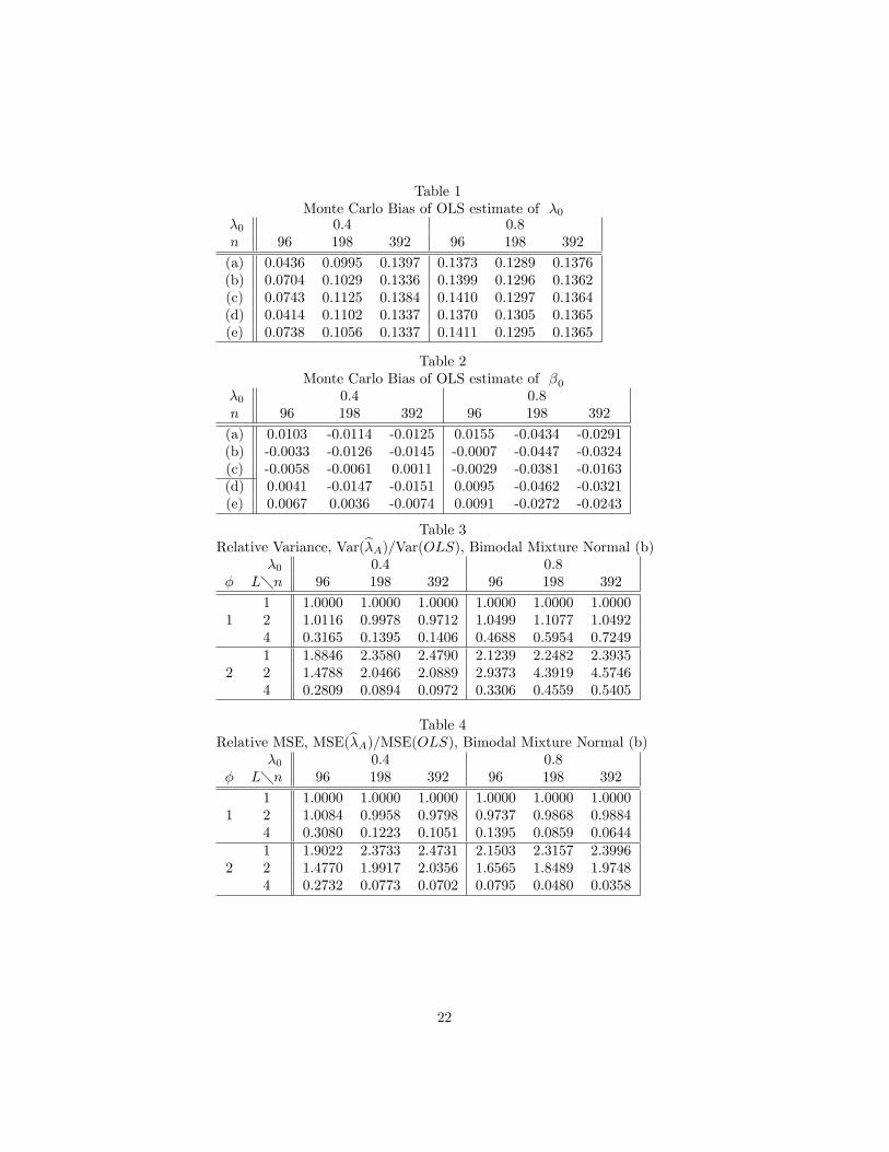
Table 1Monte Carlo Bias of OLS estimate of �0

�0 0.4 0.8n 96 198 392 96 198 392

(a) 0.0436 0.0995 0.1397 0.1373 0.1289 0.1376(b) 0.0704 0.1029 0.1336 0.1399 0.1296 0.1362(c) 0.0743 0.1125 0.1384 0.1410 0.1297 0.1364(d) 0.0414 0.1102 0.1337 0.1370 0.1305 0.1365(e) 0.0738 0.1056 0.1337 0.1411 0.1295 0.1365

Table 2Monte Carlo Bias of OLS estimate of �0

�0 0.4 0.8n 96 198 392 96 198 392

(a) 0.0103 -0.0114 -0.0125 0.0155 -0.0434 -0.0291(b) -0.0033 -0.0126 -0.0145 -0.0007 -0.0447 -0.0324(c) -0.0058 -0.0061 0.0011 -0.0029 -0.0381 -0.0163(d) 0.0041 -0.0147 -0.0151 0.0095 -0.0462 -0.0321(e) 0.0067 0.0036 -0.0074 0.0091 -0.0272 -0.0243

Table 3Relative Variance, Var(b�A)=Var(OLS), Bimodal Mixture Normal (b)

�0 0.4 0.8� L�n 96 198 392 96 198 392

1 1.0000 1.0000 1.0000 1.0000 1.0000 1.00001 2 1.0116 0.9978 0.9712 1.0499 1.1077 1.0492

4 0.3165 0.1395 0.1406 0.4688 0.5954 0.72491 1.8846 2.3580 2.4790 2.1239 2.2482 2.3935

2 2 1.4788 2.0466 2.0889 2.9373 4.3919 4.57464 0.2809 0.0894 0.0972 0.3306 0.4559 0.5405

Table 4Relative MSE, MSE(b�A)=MSE(OLS), Bimodal Mixture Normal (b)

�0 0.4 0.8� L�n 96 198 392 96 198 392

1 1.0000 1.0000 1.0000 1.0000 1.0000 1.00001 2 1.0084 0.9958 0.9798 0.9737 0.9868 0.9884

4 0.3080 0.1223 0.1051 0.1395 0.0859 0.06441 1.9022 2.3733 2.4731 2.1503 2.3157 2.3996

2 2 1.4770 1.9917 2.0356 1.6565 1.8489 1.97484 0.2732 0.0773 0.0702 0.0795 0.0480 0.0358

22

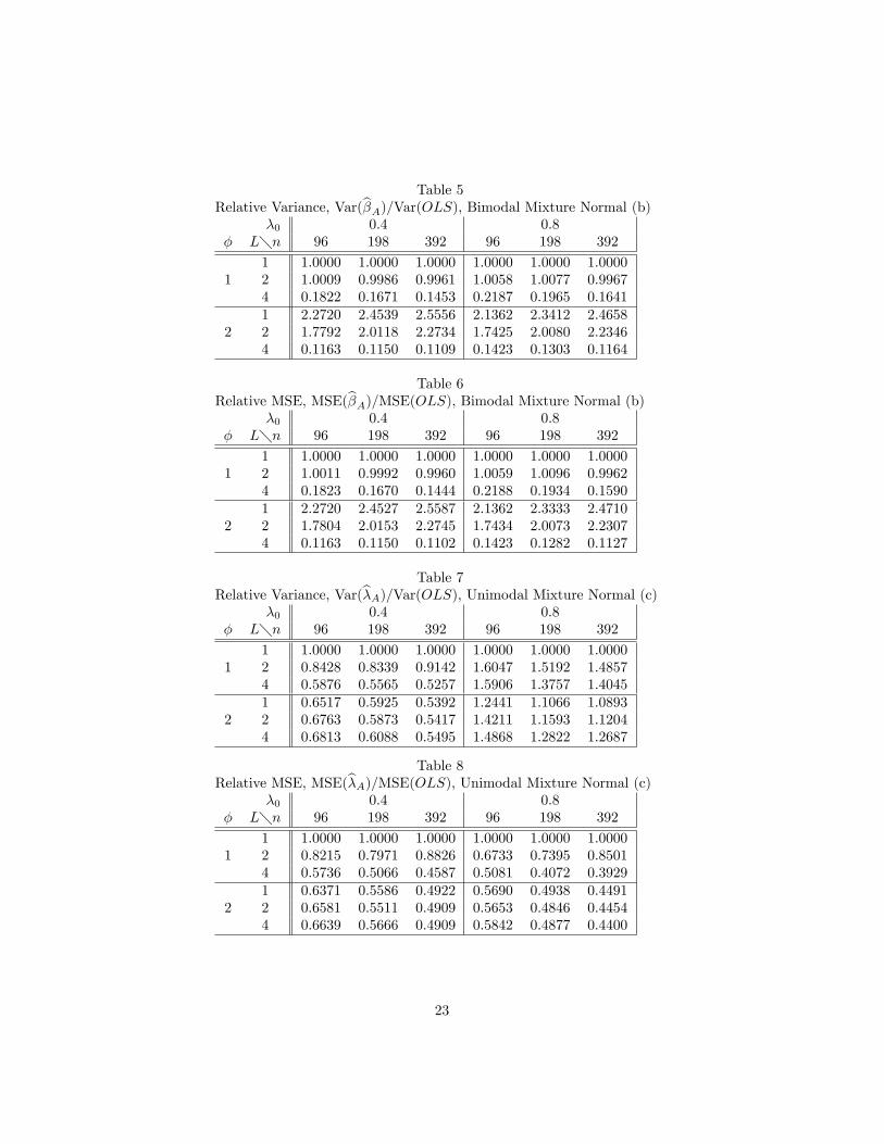
Table 5Relative Variance, Var(b�A)=Var(OLS), Bimodal Mixture Normal (b)

�0 0.4 0.8� L�n 96 198 392 96 198 392

1 1.0000 1.0000 1.0000 1.0000 1.0000 1.00001 2 1.0009 0.9986 0.9961 1.0058 1.0077 0.9967

4 0.1822 0.1671 0.1453 0.2187 0.1965 0.16411 2.2720 2.4539 2.5556 2.1362 2.3412 2.4658

2 2 1.7792 2.0118 2.2734 1.7425 2.0080 2.23464 0.1163 0.1150 0.1109 0.1423 0.1303 0.1164

Table 6Relative MSE, MSE(b�A)=MSE(OLS), Bimodal Mixture Normal (b)

�0 0.4 0.8� L�n 96 198 392 96 198 392

1 1.0000 1.0000 1.0000 1.0000 1.0000 1.00001 2 1.0011 0.9992 0.9960 1.0059 1.0096 0.9962

4 0.1823 0.1670 0.1444 0.2188 0.1934 0.15901 2.2720 2.4527 2.5587 2.1362 2.3333 2.4710

2 2 1.7804 2.0153 2.2745 1.7434 2.0073 2.23074 0.1163 0.1150 0.1102 0.1423 0.1282 0.1127

Table 7Relative Variance, Var(b�A)=Var(OLS), Unimodal Mixture Normal (c)

�0 0.4 0.8� L�n 96 198 392 96 198 392

1 1.0000 1.0000 1.0000 1.0000 1.0000 1.00001 2 0.8428 0.8339 0.9142 1.6047 1.5192 1.4857

4 0.5876 0.5565 0.5257 1.5906 1.3757 1.40451 0.6517 0.5925 0.5392 1.2441 1.1066 1.0893

2 2 0.6763 0.5873 0.5417 1.4211 1.1593 1.12044 0.6813 0.6088 0.5495 1.4868 1.2822 1.2687

Table 8Relative MSE, MSE(b�A)=MSE(OLS), Unimodal Mixture Normal (c)

�0 0.4 0.8� L�n 96 198 392 96 198 392

1 1.0000 1.0000 1.0000 1.0000 1.0000 1.00001 2 0.8215 0.7971 0.8826 0.6733 0.7395 0.8501

4 0.5736 0.5066 0.4587 0.5081 0.4072 0.39291 0.6371 0.5586 0.4922 0.5690 0.4938 0.4491

2 2 0.6581 0.5511 0.4909 0.5653 0.4846 0.44544 0.6639 0.5666 0.4909 0.5842 0.4877 0.4400

23

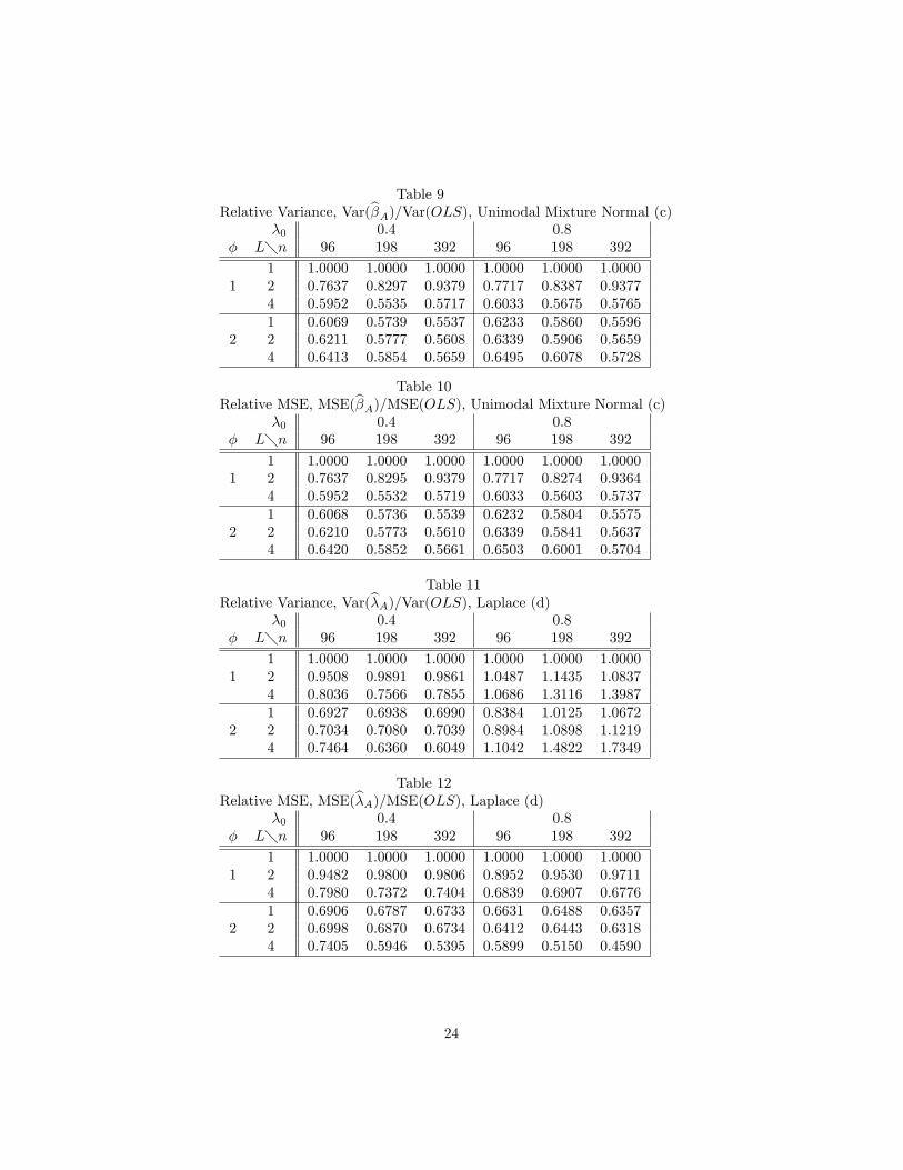
Table 9Relative Variance, Var(b�A)=Var(OLS), Unimodal Mixture Normal (c)

�0 0.4 0.8� L�n 96 198 392 96 198 392

1 1.0000 1.0000 1.0000 1.0000 1.0000 1.00001 2 0.7637 0.8297 0.9379 0.7717 0.8387 0.9377

4 0.5952 0.5535 0.5717 0.6033 0.5675 0.57651 0.6069 0.5739 0.5537 0.6233 0.5860 0.5596

2 2 0.6211 0.5777 0.5608 0.6339 0.5906 0.56594 0.6413 0.5854 0.5659 0.6495 0.6078 0.5728

Table 10Relative MSE, MSE(b�A)=MSE(OLS), Unimodal Mixture Normal (c)

�0 0.4 0.8� L�n 96 198 392 96 198 392

1 1.0000 1.0000 1.0000 1.0000 1.0000 1.00001 2 0.7637 0.8295 0.9379 0.7717 0.8274 0.9364

4 0.5952 0.5532 0.5719 0.6033 0.5603 0.57371 0.6068 0.5736 0.5539 0.6232 0.5804 0.5575

2 2 0.6210 0.5773 0.5610 0.6339 0.5841 0.56374 0.6420 0.5852 0.5661 0.6503 0.6001 0.5704

Table 11Relative Variance, Var(b�A)=Var(OLS), Laplace (d)

�0 0.4 0.8� L�n 96 198 392 96 198 392

1 1.0000 1.0000 1.0000 1.0000 1.0000 1.00001 2 0.9508 0.9891 0.9861 1.0487 1.1435 1.0837

4 0.8036 0.7566 0.7855 1.0686 1.3116 1.39871 0.6927 0.6938 0.6990 0.8384 1.0125 1.0672

2 2 0.7034 0.7080 0.7039 0.8984 1.0898 1.12194 0.7464 0.6360 0.6049 1.1042 1.4822 1.7349

Table 12Relative MSE, MSE(b�A)=MSE(OLS), Laplace (d)

�0 0.4 0.8� L�n 96 198 392 96 198 392

1 1.0000 1.0000 1.0000 1.0000 1.0000 1.00001 2 0.9482 0.9800 0.9806 0.8952 0.9530 0.9711

4 0.7980 0.7372 0.7404 0.6839 0.6907 0.67761 0.6906 0.6787 0.6733 0.6631 0.6488 0.6357

2 2 0.6998 0.6870 0.6734 0.6412 0.6443 0.63184 0.7405 0.5946 0.5395 0.5899 0.5150 0.4590

24

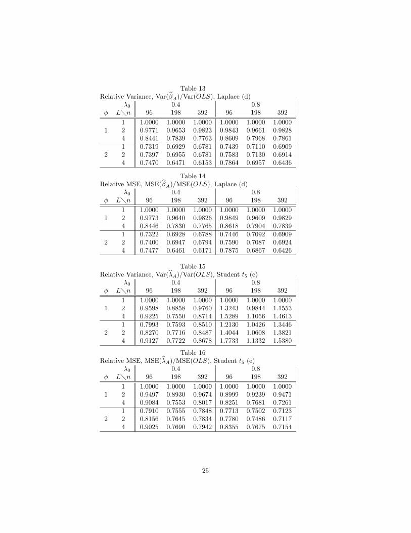
Table 13Relative Variance, Var(b�A)=Var(OLS), Laplace (d)

�0 0.4 0.8� L�n 96 198 392 96 198 392

1 1.0000 1.0000 1.0000 1.0000 1.0000 1.00001 2 0.9771 0.9653 0.9823 0.9843 0.9661 0.9828

4 0.8441 0.7839 0.7763 0.8609 0.7968 0.78611 0.7319 0.6929 0.6781 0.7439 0.7110 0.6909

2 2 0.7397 0.6955 0.6781 0.7583 0.7130 0.69144 0.7470 0.6471 0.6153 0.7864 0.6957 0.6436

Table 14Relative MSE, MSE(b�A)=MSE(OLS), Laplace (d)

�0 0.4 0.8� L�n 96 198 392 96 198 392

1 1.0000 1.0000 1.0000 1.0000 1.0000 1.00001 2 0.9773 0.9640 0.9826 0.9849 0.9609 0.9829

4 0.8446 0.7830 0.7765 0.8618 0.7904 0.78391 0.7322 0.6928 0.6788 0.7446 0.7092 0.6909

2 2 0.7400 0.6947 0.6794 0.7590 0.7087 0.69244 0.7477 0.6461 0.6171 0.7875 0.6867 0.6426

Table 15Relative Variance, Var(b�A)=Var(OLS), Student t5 (e)

�0 0.4 0.8� L�n 96 198 392 96 198 392

1 1.0000 1.0000 1.0000 1.0000 1.0000 1.00001 2 0.9598 0.8858 0.9760 1.3243 0.9844 1.1553

4 0.9225 0.7550 0.8714 1.5289 1.1056 1.46131 0.7993 0.7593 0.8510 1.2130 1.0426 1.3446

2 2 0.8270 0.7716 0.8487 1.4044 1.0608 1.38214 0.9127 0.7722 0.8678 1.7733 1.1332 1.5380

Table 16Relative MSE, MSE(b�A)=MSE(OLS), Student t5 (e)

�0 0.4 0.8� L�n 96 198 392 96 198 392

1 1.0000 1.0000 1.0000 1.0000 1.0000 1.00001 2 0.9497 0.8930 0.9674 0.8999 0.9239 0.9471

4 0.9084 0.7553 0.8017 0.8251 0.7681 0.72611 0.7910 0.7555 0.7848 0.7713 0.7502 0.7123

2 2 0.8156 0.7645 0.7834 0.7780 0.7486 0.71174 0.9025 0.7690 0.7942 0.8355 0.7675 0.7154

25

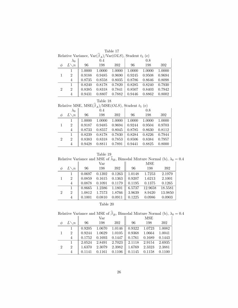
Table 17Relative Variance, Var(b�A)=Var(OLS), Student t5 (e)

�0 0.4 0.8� L�n 96 198 392 96 198 392

1 1.0000 1.0000 1.0000 1.0000 1.0000 1.00001 2 0.9188 0.9485 0.9690 0.9245 0.9508 0.9694

4 0.8735 0.8558 0.8035 0.8786 0.8646 0.80981 0.8240 0.8178 0.7820 0.8285 0.8240 0.7930

2 2 0.8385 0.8318 0.7841 0.8507 0.8403 0.79424 0.9431 0.8807 0.7882 0.9446 0.8862 0.8002

Table 18Relative MSE, MSE(b�A)=MSE(OLS), Student t5 (e)

�0 0.4 0.8� L�n 96 198 392 96 198 392

1 1.0000 1.0000 1.0000 1.0000 1.0000 1.00001 2 0.9187 0.9485 0.9694 0.9244 0.9504 0.9703

4 0.8733 0.8557 0.8045 0.8785 0.8630 0.81121 0.8239 0.8178 0.7830 0.8284 0.8226 0.7944

2 2 0.8383 0.8318 0.7853 0.8506 0.8384 0.79574 0.9428 0.8811 0.7891 0.9441 0.8825 0.8000

Table 19Relative Variance and MSE of b�B , Bimodal Mixture Normal (b), �0 = 0:4

Var� L�n 96 198 392

1 0.0697 0.1392 0.12631 2 0.0859 0.1615 0.1363

4 0.0878 0.1091 0.11791 0.8665 1.2386 1.1801

2 2 1.0812 1.7573 1.87664 0.1001 0.0810 0.0911

MSE96 198 392

1.0148 1.7253 2.19790.9207 1.6213 2.10010.1195 0.1375 0.12656.5737 12.9658 18.55813.9639 8.9420 13.98500.1225 0.0986 0.0903

Table 20

Relative Variance and MSE of b�B , Bimodal Mixture Normal (b), �0 = 0:4Var

� L�n 96 198 392

1 0.9205 1.0670 1.01461 2 0.9244 1.0629 1.0105

4 0.1752 0.1693 0.14471 2.0524 2.8491 2.7023

2 2 1.6370 2.3079 2.39824 0.1141 0.1161 0.1106

MSE96 198 392

0.9322 1.0723 1.00820.9368 1.0664 1.00410.1761 0.1689 0.14432.1118 2.9154 2.69351.6769 2.3323 2.38810.1145 0.1158 0.1100

26

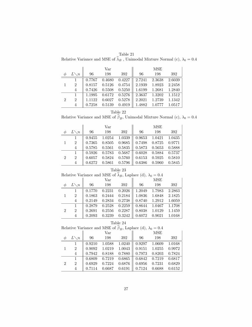
Table 21Relative Variance and MSE of b�B , Unimodal Mixture Normal (c), �0 = 0:4

Var� L�n 96 198 392

1 0.7767 0.4680 0.42271 2 0.8157 0.5126 0.4754

4 0.7426 0.5508 0.52501 1.1995 0.6172 0.5276

2 2 1.1122 0.6027 0.52784 0.7258 0.5139 0.4919

MSE96 198 392

2.7241 2.3638 2.60392.1939 1.8923 2.24581.6199 1.2681 1.28402.3637 1.3202 1.15122.2021 1.2739 1.13421.4882 1.0777 1.0517

Table 22Relative Variance and MSE of b�B , Unimodal Mixture Normal (c), �0 = 0:4

Var� L�n 96 198 392

1 0.9455 1.0254 1.03391 2 0.7365 0.8505 0.9685

4 0.5785 0.5561 0.58351 0.5926 0.5783 0.5687

2 2 0.6057 0.5824 0.57604 0.6272 0.5861 0.5796

MSE96 198 392

0.9653 1.0421 1.04350.7498 0.8725 0.97710.5873 0.5653 0.58880.6028 0.5884 0.57370.6153 0.5925 0.58100.6386 0.5960 0.5845

Table 23Relative Variance and MSE of b�B ; Laplace (d), �0 = 0:4

Var� L�n 96 198 392

1 0.1770 0.2231 0.20261 2 0.1863 0.2444 0.2184

4 0.2149 0.2834 0.27381 0.2879 0.2528 0.2259

2 2 0.2691 0.2556 0.22874 0.2093 0.3239 0.3242

MSE96 198 392

1.2049 1.7983 2.28631.0836 1.6848 2.18250.8740 1.2912 1.60590.8644 1.0467 1.17080.8038 1.0129 1.14590.6072 0.9021 1.0168

Table 24Relative Variance and MSE of b�B ; Laplace (d), �0 = 0:4

Var� L�n 96 198 392

1 0.9210 1.0588 1.02401 2 0.9092 1.0219 1.0043

4 0.7942 0.8188 0.78801 0.6809 0.7219 0.6865

2 2 0.6929 0.7224 0.68764 0.7114 0.6687 0.6191

MSE96 198 392

0.9297 1.0609 1.01680.9151 1.0255 0.99720.7973 0.8203 0.78240.6842 0.7219 0.68170.6956 0.7231 0.68290.7124 0.6688 0.6152

27

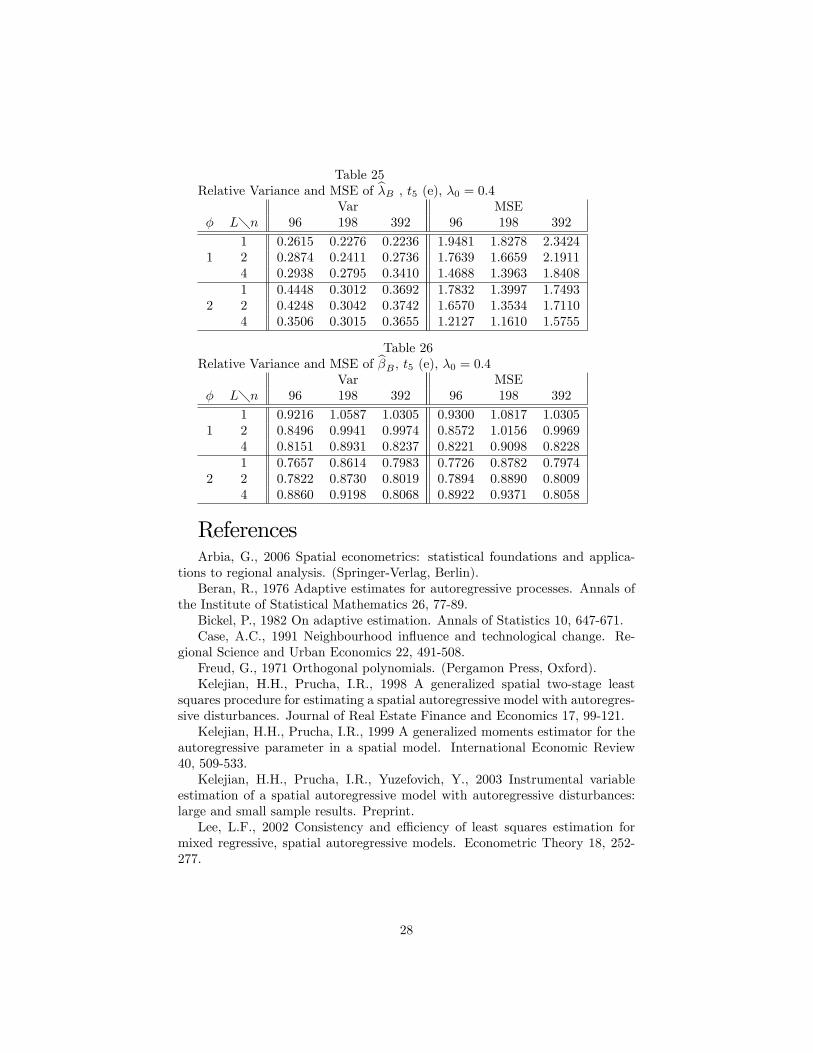
Table 25Relative Variance and MSE of b�B , t5 (e), �0 = 0:4

Var� L�n 96 198 392

1 0.2615 0.2276 0.22361 2 0.2874 0.2411 0.2736

4 0.2938 0.2795 0.34101 0.4448 0.3012 0.3692

2 2 0.4248 0.3042 0.37424 0.3506 0.3015 0.3655

MSE96 198 392

1.9481 1.8278 2.34241.7639 1.6659 2.19111.4688 1.3963 1.84081.7832 1.3997 1.74931.6570 1.3534 1.71101.2127 1.1610 1.5755

Table 26Relative Variance and MSE of b�B ; t5 (e), �0 = 0:4

Var� L�n 96 198 392

1 0.9216 1.0587 1.03051 2 0.8496 0.9941 0.9974

4 0.8151 0.8931 0.82371 0.7657 0.8614 0.7983

2 2 0.7822 0.8730 0.80194 0.8860 0.9198 0.8068

MSE96 198 392

0.9300 1.0817 1.03050.8572 1.0156 0.99690.8221 0.9098 0.82280.7726 0.8782 0.79740.7894 0.8890 0.80090.8922 0.9371 0.8058

ReferencesArbia, G., 2006 Spatial econometrics: statistical foundations and applica-

tions to regional analysis. (Springer-Verlag, Berlin).Beran, R., 1976 Adaptive estimates for autoregressive processes. Annals of

the Institute of Statistical Mathematics 26, 77-89.Bickel, P., 1982 On adaptive estimation. Annals of Statistics 10, 647-671.Case, A.C., 1991 Neighbourhood in�uence and technological change. Re-

gional Science and Urban Economics 22, 491-508.Freud, G., 1971 Orthogonal polynomials. (Pergamon Press, Oxford).Kelejian, H.H., Prucha, I.R., 1998 A generalized spatial two-stage least

squares procedure for estimating a spatial autoregressive model with autoregres-sive disturbances. Journal of Real Estate Finance and Economics 17, 99-121.Kelejian, H.H., Prucha, I.R., 1999 A generalized moments estimator for the

autoregressive parameter in a spatial model. International Economic Review40, 509-533.Kelejian, H.H., Prucha, I.R., Yuzefovich, Y., 2003 Instrumental variable

estimation of a spatial autoregressive model with autoregressive disturbances:large and small sample results. Preprint.Lee, L.F., 2002 Consistency and e¢ ciency of least squares estimation for

mixed regressive, spatial autoregressive models. Econometric Theory 18, 252-277.

28

Lee, L.F., 2003 Best spatial two-stage least squares estimators for a spatialautoregressive model with autoregressive disturbances. Econometric Reviews22, 307-335.Lee, L.F., 2004 Asymptotic distributions of quasi-maximum likelihood esti-

mates for spatial autoregressive models. Econometrica 72, 1899-1925.Newey, W.K., 1988 Adaptive estimation of regression models via moment

restrictions. Journal of Econometrics 38, 301-339.Robinson, P.M., 1988 The stochastic di¤erence between econometric statis-

tics. Econometrica 56, 531-548.Robinson, P.M., 2005 E¢ ciency improvements in inference on stationary and

nonstationary fractional time series. Annals of Statistics 33, 1800-1842.Stone, C.J., 1975 Adaptive maximum likelihood estimators of a location

parameter. Annals of Statistics 2, 267-289.Whittle, P., 1954 On stationary processes in the plane. Biometrika 41, 434-

449.

29