Effects of the Built Environment on Childhood Obesity:

The Case of Urban Recreation Trails and Crime1

by

Robert Sandy#, Rusty Tchernis*, Jeff Wilson‡, John Ottensmann**, Gilbert Liu##, and Xilin Zhou†

November 8, 2010

Abstract

We study the effects urban environment on childhood obesity by concentrating on the effects of walking trails and crime close to child’s home on their BMI and obesity status. We use a unique dataset, which combines information on recreation trails in Indianapolis with data on violent crimes and anthropomorphic and diagnostic data from children’s clinic visits between 1996 and 2005. We find that having a trail near a home reduces children’s weight. However, the effect depends on the amount of nearby violent crimes and significant reductions occur only in low crime areas and could result in opposite effects on weight in high crime areas. These effects are primarily among boys, older children, and children who live in higher income neighborhoods. Evaluated at the mean length of trails this effect for older children in no crime areas would be a reduction of two pounds. In addition, when we do a falsification test using planned trails instead of existing trails we find that trails are locating in areas with heavier children suggesting that our results on effects of trails represent a lower bound.

#Department of Economics, IUPUI *Department of Economics, Georgia State University and NBER ‡Department of Geography, IUPUI **SchoolofPublicandEnvironmentalAffairs,IUPUI ## Department of Pediatrics, Indiana University School of Medicine † Department of Economics, Georgia State University

1We thank Shawn Hoch, Zhang Ya, Megan McDermott, Bikul Tulachan, Jonathan Raymont for research assistance. This study was funded under NIH NIDDK grant R21 DK075577-01. We thank Kristen Butcher, Daniel Millimet, and seminar participants at GSU and IUPUI for suggestions and comments. Address for correspondence: Rusty Tchernis, Department of Economics, Andrew Young School of Policy Studies, Georgia State University, P.O. Box 3992, Atlanta, GA 30302-3992, USA. E-mail: ecort@langate.gsu.edu

2

Introduction:

The extent and the dire health consequences of the U.S. child obesity epidemic are

well documented (Anderson and Whitaker 2009, Hannon et al. 2005). The alarming growth in

child obesity has generated many proposals, some of which have been implemented at local

and state levels. These proposals have been primarily aimed at schools and food sellers. They

include: state and national taxes on sugared soft drinks (Salant 2009), bans on such drinks in

schools (Price 2006), bans on building new fast food restaurants, increases in mandatory

physical education requirements, and healthier school lunch menus (Trust for America’s

Health 2009). Almost all of these proposals have been made in the absence of evidence that

they would have a beneficial effect or in spite of evidence that they would have no benefit.

Doubts about the effectiveness of specific mechanisms for countering child or adult obesity

have been raised by: Cawley et al. (2007) on physical education classes; Millimet et al. (2007)

changing school lunch programs; Sandy et al. (2009) and Anderson and Matsa (2007) on bans

on new fast food restaurants; and, Whatley Blum et al. (2008) on banning sugared soft drinks.

There have been proposals to use differential health insurance pricing to reduce adult

obesity (Johnson 2009). For adults with any health insurance an obesity surcharge on their

health insurance premium is similar to a direct tax for being obese. However, even if they

might be effective in altering parents’ child-rearing behavior, applying differential health

insurance pricing to children or limiting their access to health insurance is unlikely to be

politically feasible. An incident that occurred in October of 2009 illustrates the public’s

reaction. A private insurer, the Rocky Mountain Health Plan, refused to sell health insurance

to a Colorado family on the grounds that the family’s four-month old baby was obese

(Lofholm 2009). Within two days a tsunami of national unfavorable publicity caused the

company to reverse its decision (Sandell 2009). It is similarly difficult to find politically

feasible policies to reduce children’s at home sedentary activities, such as television viewing

or playing video games. Obesity report cards, i.e. reports on the child’s BMI percentile sent

from schools to a child’s parents, are an example of a policy that tries to reach into the child’s

home. Obesity reports cards have generated a great deal of resistance (Kantor 2007).

3

Reversing the child obesity epidemic requires policies that are both effective and

politically feasible. A broad category of potential interventions is the built environment

around the children’s homes. The aforementioned ban on the construction of new fast food

restaurants is an example of altering the built environment to reduce obesity. Subsidies for or

public provision of potentially weight-reducing built amenities would be much easier to

implement than either differential pricing of health insurance for children or obesity report

cards. An additional advantage of weight-reducing recreational amenities is that they have

smaller negative spillovers on individuals who are at healthy weights. While individuals who

are in a healthy weight range would be taxed to support the recreational amenities, they are at

least as likely to use them as obese individuals. In contrast, taxes on sugared soft drinks and

bans on fast food restaurants have substantial spillovers on the non-obese.

Proposals for altering the built environment run the gamut from adding sidewalks to

encourage walking to such recreational amenities as pools, soccer fields, basketball courts,

and trails, to zoning laws requiring mixes of residences and retail outlets, to locating schools

within walking distance of the homes (King et al. 1995, Sallis 1998, Margetts 2004).

Proposals addressing the built environment are also running well ahead of the evidence.

Although the American Academy of Pediatrics Committee on Environment recommendations

include: “Fund research on the impact of the built environment at neighborhood and

community levels on the promotion of overall health and active lifestyles for children and

families” it nevertheless recommends a host of interventions that have little empirical support

(Committee on Environmental Health 2009).

A crucial problem for identifying public policies that can counter the child obesity

epidemic via the built environment is the endogeneity of household and amenity location

choices. Households who chose to live near an amenity would be expected to have stronger

preferences for that amenity. Moreover, the locations of public recreational amenities are a

political decision that can be influenced by the lobbying of the households most interested in

using the amenity. Thus, cross-sectional studies of built environment may reveal more about

the preferences of the families who live near an amenity than they reveal about its impact.

Private companies, such as fast food restaurants, place outlets where, ceteris paribus, they

4

expect to have the most customers. An example of this endogeneity problem is the

conclusion, formed on the basis of many cross-sectional studies, that urban sprawl contributes

to obesity. This result was not supported in either a study of people who moved between

cities with different levels of sprawl (Plantinga and Bernell 2007) or in a study of changes in

the level of sprawl over time in a given city (Ewing et al. 2006).

The amenity that is the subject of this paper, recreation trails, presumably attracts

families to locate nearby who value a trail as an exercise opportunity. These households

would most likely have healthier diets and engage in more exercise than the average

household, even without a nearby trail. Absent the random assignment of residential location,

such as the Moving to Opportunity Experiment (Kling 2004), an ideal research design is to

either have an instrument that predicts location but not BMI or a natural experiment that

moves households or amenities. Since body weight is influenced by so many factors it is

difficult to find a plausible instrument. Some natural experiments that have moved many

households, e.g. Hurricane Katrina, also change other factors that are related to body weight.

If the subjects of the natural experiment are clinically depressed it is difficult to say what their

new recreational amenities did to their weights.

In this paper we take advantage of the fact that the recreation trails in the City of

Indianapolis had to be located on city owned land along an abandoned rail line or along

several streams and rivers. That limited the usual political influence in public amenity

locations. Also, given the short times between their announcement and construction, these

trails could not have been factored into the location choices of most of the families who live

nearby. An additional advantage of studying these trails is that they run through a variety of

areas in terms of income, housing types, and land use. Our clinical data on children yielded a

reasonably large sample of approximately 97,000 observations on children’s BMI for

approximately 37,000 children.

Our initial research plan was to utilize a fixed effects model to estimate the impact on

BMI of a trail being created near a given child’s home. However, we had pre and post-trail

arrival biometric measures on too few children who gained a trail while residing at the same

5

address. Instead, we use fixed effects at census tract lever and compare the results for children

who changed addresses at any time over their duration of clinic visits to those with stable

addresses. We find little difference between families who changed address and those with

fixed address and results for the stayers give us confidence that recreation trails do reduce

child obesity. The effects vary by age and gender, with older children and boys having the

greatest benefit.

Any beneficial effects of a recreation trail depended on the nearby rates of violent

crime. In above median crime areas the trails have no weight effects. Within below median

crime areas trails have weight reducing benefits. Lastly, violent crimes alone appear to

significantly raise children’s weights, with or without a nearby trail. While we are not sure if

that is the direct effect of crime or other characteristics of areas with more crime, we find

these findings interesting. In addition, these results are strongest for the younger children and

for girls.

The balance of this paper discusses: 1) the literature on the body weight effects of the

built environment, 2) data used in this paper. 3) estimation strategy, 4) results, and 5)

conclusions.

Literature Review

Obesity epidemic has become a growing public concern. The models of “obesogenic

environment” propose a causal relationship between environmental characteristics and obesity

(Egger and Swinburn 1997, Hill and Peters 1998, Poston and Foreyt 1999, Swinburn and

Egger 1999). Contemporary literature is generally concerned with two aspects of the causal

relationship. One set of studies focuses on the influences of the built environment

(transportation, physical activities facilities, and local food environment etc.) on obesity

(Ewing et al. 2006, Booth et al. 2005, French et al. 2000). Another set of studies concentrates

on the impact of socioeconomic deprivation of the community on obesity (Oliver and Hayes

2005, Liu et al. 2002, Gordon-Larsen et al. 2006).

6

Among the influential environmental aspects, one key factor is the effect of

unfavorable neighborhood characteristics for physical activities. The modern urban design

mainly facilitates the automotive transportation (Saelens et al. 2003, Frank et al. 2004, Ewing

et al. 2003, Jackson and Kochtitzky 2002). It brings us convenience; however, it also pushes

us toward a more and more sedentary lifestyle (Nelson and Gordon-Larsen 2006, Boone et al.

2007).

Many studies have investigated the relationship between built environmental

characteristics and obesity. Burdette and Whitaker (2004) explored the bodyweights of low-

income children in a cross-sectional study. They found that accessibility of playgrounds and

fast food restaurants, and the level of neighborhood safety didn’t associate with children’s

overweight status. Hinkley et al. (2008) reviewed articles investigating the determinants of

preschool children’s physical activities, and found that BMI has no association with physical

activity. Sen et al. (2009) utilized mothers’ self-reported measures of neighborhood quality to

examine whether there was any relationship between children’s BMI and the built

environment. They found that overall neighborhood quality didn’t significantly relate to

children’s bodyweight. However, their results showed that mothers’ perception of

neighborhood safety has important influence on Children’s BMI.

However, Sandy et al. (2009) used panel dataset of clinical records to investigate

whether changes in nearby physical or social environmental factors could be the reason for

changes in child weight. They found amenities, including fitness areas, kickball diamonds,

and volleyball courts, help to reduce children’s BMI. Stafford et al. (2008) utilized a structural

equation modeling approach to explore the causal relationship between neighborhood

characteristics and obesity. They found that BMI was negatively related to physical activity

participations, though they couldn’t claim that this correlation was causal. In 2006 Gordon-

Larsen et al. found in a cross-section analysis that, children who grew up in neighborhoods

with more recreational facilities within a 5-mile buffer around the child’s home had a lower

probability of being overweight. Many researchers agree that living in a walking-friendly

neighborhood is beneficial to residents’ health (Li et al. 2005, Giles-Corti et al. 2003).

7

The utilization of community facilities is closely related with neighborhood safety.

According to a report concerning neighborhood safety and physical inactivity by CDC (1999),

residents are significantly less active in less safe neighborhoods than residents are in more

safe neighborhoods. Neighborhood insecurity impedes physical activities (Romero et al 2001,

Duncan et al 2009). Even without considering physical activity, safety could be considered to

be an independent factor that correlates with obesity. Parents’ perceptions of sound

neighborhood safety are associated with less obesity risk (Lumeng et al 2006, Burdette,

Wadden and Whitaker 2006).

The present study singles out the recreation trails as a particular environmental factor,

which may have correlation with physical activities. As stated in the previous part, the

advantage of using trails as built environmental indicators is that, the allocations of trails in

Indianapolis could be considered as “exogenous” to subjective decisions. Of the seventeen

amenities in Sandy et al. (2009), the trails were the least likely to have locations dictated by

either neighborhood politics or private information. It is clear in Figure 1 that, most trails

within Indianapolis locate along waterways, except some waterways along the western and

eastern boundaries which are thinly populated. There is also a trail placed on an unused

railroad track which is the vertical trail segment labeled as the Monon Trail.

Another advantage to study trails is their popularity, and their commonly agreed

positive effects on promoting walking and cycling (Merom et al. 2003, Librett et al. 2006).

Trails are being heavily used in Indiana (Lindsey et al. 2002). The Monon Trail has been

described as perhaps the most heavily used urban recreation trail in the United States

(Ottensmann and Lindsey 2008, Reynolds et al. 2007). If a recreation trail had a beneficial

effect we would expect it to show up in these data.

Data:

Figure 2 shows the locations of children’s residences superimposed on the trails in

Figure 1. A gray dot indicates a single residence. Shaded gray areas indicate groups of

residences that are too close to each other to individually distinguish. The blue shading shows

8

the residential locations of children who live within a quarter mile of a trail. To make it

impossible to identify actual addresses each dot on the map was randomly shifted a small

distance. The data used in the regressions used the actual point locations.

Themainsourcesofourdataare:(1)clinicalrecordsfrompediatricambulatory

visitstotheIndianaUniversityMedicalGroupbetween1996and2005;(2)reportsof

violentcrimesfromtheIndianapolisPoliceDepartmentandtheMarionCountySheriff’s

Department;(3)dataontheinitialyearandthelengthoftrailswithinaquartermileof

thechild’shome.Thesedatasourcesaredescribedinmoredetailbelow.

(1)Clinicalrecords

TheRegenstriefMedicalRecordsSystem(RMRS),inexistencesince1974,isan

electronicversionofthepapermedicalchart.Ithasnowcapturedandstored200

milliontemporalobservationsforover1.5millionpatients.BecauseRMRSdataareboth

archivedandretrievable,investigatorsmayusethesedatatoperformretrospectiveand

prospectiveresearch.TheRMRSisdistributedacross3medicalcenters,30ambulatory

clinics,andalloftheemergencydepartmentsthroughoutthegreaterIndianapolis

region.RMRSsupportsphysicianorderentry,decisionsupport,andclinicalnoting,and

isoneofthemostsophisticatedandmostevaluatedelectronicmedicalrecordsystems

intheworld.

UsingtheRMRS,weidentifiedmedicalrecordsinwhichtherearesimultaneous

assessmentsofheightandweightinoutpatientclinicsforchildrenages3‐18years

inclusive.Fortheseclinicvisits,weextractedthevisitdate,birthdate,sex,race,

insurancestatus,andvisittype(e.g.periodichealthmaintenanceversusacutecare).We

foundthattoofewpatientshadprivateinsuranceforthisvariabletohaveanypredictive

power.Becauseheightandweightmeasurementsareroutinelyperformedaspartof

pediatrichealthmaintenance,thesemeasuresshouldbepresentforvirtuallyallchildren

receivingpreventivecareateachofthestudysites.Thedatageneratedbypediatric

visitsintheRMRSincludehigherrepresentationoflow‐incomeandminority

householdscomparedtothedemographicsofthestudyareabecausetheassociated

clinicsserveapopulationthatismostlypubliclyinsuredorhasnoinsurance.

9

Theinitialagerangeofsubjectsinthisstudyisthreetoeighteenyears.National

guidelinesforwell‐childvisitsadvocateannualvisitsbetweenages3‐6yearsandatleast

biannualvisitsthereafter.Weobservedmuchmorefrequentwell‐childvisitsforgirls

age16orabovethanforboys,presumablybecausetheformeroftenusethesevisitsto

obtaingynecologiccare,suchasaprescriptionforcontraception.WeextractedICD‐9

codesorotherdiagnoseslistdataforidentifyingchildrenwhomayhavesystematicbias

ingrowthorweightstatus(i.e.pregnancy,endocrinedisorders,cancer,congenitalheart

disease,chromosomaldisorders,andmetabolicdisorders),andexcludedobservations

forsuchchildren.Wealsoexcludedpatientencounterspriorto1996becausetheRMRS

didnotarchiveaddressdatabeforethisdate.

(2)RecreationTrails

TheIndianapolisParksandRecreationDepartmentprovideddataontheopening

dateofeachsegmentofeachtrail.Figure3showsthedateofopeningofeachtrail

segment.Theopeningdatesareallrecent.Thus,itishighlyunlikelythatmuchofthe

patternofresidentiallocationamongthestayerswhomwefirstobserveinclinicvisits

shortlyafterthetrailsopenwasinfluencedbythepresenceofatrail.

Trailaccessmetrics:

Wecreatedameasureofthelengthofanytrails,trails4,scaledper100meters,

withinacircleofradius0.25milescenteredonthechild’shome.Theminimumvaluefor

thisvariablewas0forchildrenrepresentedbythegraydotsorgrayshadinginFigure2.

Themeanamountacrossallchildrenwithorwithoutanearbytrailwas0.122,i.e.12.2

meters.Themaximumlengthwas8.44,i.e.844meters.Wealsocreatedavariablethat

measuredthelengthofanyplannedbutnotyetconstructedtrails,pl_trails4,again

scaledper100meters.Thisvariabletakesthevaluezerowhennotrailwasplannedand

whenatrailalreadyexists.

Thereisnoestablishedmetricforrepresentingtrailavailability.Itisnotclear

thatlivingimmediatelyadjacenttoatrailthatfollowsastraightlineprovidesanylessof

arecreationalopportunitythanlivingimmediatelyadjacenttoatrailthatfollowsa

zigzagpath.Ourlength‐within‐a‐circlemetrictreatsazigzaggingtrailasprovidingmore

recreationalopportunitythanastraight‐linetrailwhenbothareadjacenttothechild’s

10

home.However,mostofthechildrenwholivenearatrailarenearsegmentsthatare

reasonablyapproximatedasastraightline.Togetasenseofhowcirclesof0.25‐mile

radiuswouldfitintoFigures1and2,Indianapolisisapproximatedbyasquareof20

milesoneachside.Thus,eventhetrailsalongwindingpathsnexttoriversare

reasonablyapproximatedbyastraightwithinthesesmallcircles.

Weexperimentedwithdifferentmetricsincludingadummyvariableforhaving

anytrailandacountforthenumberoftrails(somechildrenlivednearintersectionsof

trails).Thedistancewithinthecirclemetricperformedbetterthanthedummyorthe

count.Wealsoexperimentedwiththesquareofthedistancetoseeiftherewasanon‐

lineareffecttolengthofnearbytrails.Itwasnotsignificantinanyspecification.Wehave

approximately6,600biometricobservationsonapproximately1,800childrenwhohada

trailwithinaquartermile.

(3)Crimedata

Duringthestudyperiod,theprimarylawenforcementresponsibilityforMarion

CountywasdividedbetweentheIndianapolisPoliceDepartment(IPD),whichhad

responsibilityfortheareawithintheoriginalIndianapolisboundary,theMarionCounty

Sheriff’sDepartment(MCSD),whichhadresponsibilityformostoftheoutlyingareasof

thecounty,andthepolicedepartmentsofthefoursmallexcludedmunicipalitiesof

Speedway,Lawrence,Southport,andBeechGrove.WhenthecitylimitsofIndianapolis

wereexpandedtotheborderofMarionCountyin1970,theoriginalpolicejurisdictions

werenotaffected.In2007theIndianapolisPoliceDepartmentandtheMarionCounty

Sheriff’sDepartmentweremergedintotheIndianapolisMetropolitanPolice

Department.

FromtheIndianapolisPoliceDepartment,fortheIPDserviceareainwhichthey

hadprimaryresponsibility,wehaveadatasetofthegeocodedlocationsofallcrimes

reportedfortheFederalBureauofInvestigation’sUniformCrimeReports(UCR),from

1992through2005.FromtheMarionCountySheriff’sDepartment,fortheareainwhich

theyhadprimaryresponsibility,wehaveadatasetonthepointlocationsofawiderange

ofcrimesandotherincidents,includingtheUCRcrimes,from2000through2005.We

areusinginformationonthecrimesfrombothdatasetsthatareincludedintheUCR

11

violentcrimecategories:criminalhomicides,rapes,robberies,andaggravatedassaults.

Thedatasetincludesthedateandtimeofthecrime,andmoredetailedinformationon

thespecifictypeofcrimewithineachofthosefourcategories.Becauseofthemannerin

whichthesedatahavebeenassembled,wehavereasontobelievethattheseare

accuratelocationsandthattheclassificationofthetypeofcrimeisaccurate.

Tosummarize,wehavethefollowingcoverageforviolentcrimes:

1)Upthrough1999,fortheIPDserviceareaonly.

2)From2000through2005,forboththeIPDserviceareaandtheMCSD

jurisdiction.

Nocrimedataareavailableforanytimeperiodforthejurisdictionsofthefour

smallexcludedmunicipalitiesthatarewithinMarionCounty.

Datacleaning

Inexaminingtheheightandweightdatafromtheclinicalrecordswefound

highly‐improbablepatterns,suchasachildshrinkingfiveinchesinheightfromone

well‐childvisittothenext.Wecalculatedz‐scoresforheightandweightmeasuresbased

onyear2000USCentersforDiseaseControlandPrevention(CDC)growthcharts.We

usedCDCstatisticalprogramstoidentifybiologically‐implausiblevaluesforheightsand

weights(CDC,2000).Figure4showsthehistogramsofheightsandweights,excluding

biologically‐implausiblevalueswithz‐scoresgreaterthan+3.0.

Visually,thereisasmallamountoftruncationfortheheightsintherighttailof

theheightdistribution.Ascanbeseeninthesecondgraph,thetruncationintheright

tailofthebodyweightdistributionissubstantialandmayreflectinappropriate

exclusionofhighweight‐for‐agechildren.TheCDCGrowthChartreferencepopulation

spanstheperiod1963to1994,andthusdoesnotfullycovertheepidemicinchild

obesityofthepasttwodecades.Anothervisualindicatoroftheextentoftheepidemicis

howmuchthedistributionhasshiftedtotherightrelativetothemeanofthereference

population.Wetreatedobservationswithweight‐for‐heightandweight‐for‐agez‐scores

equaltoorexceeding+5.0asoutlierslikelyresultingfromdataentryerroror

measurementerrors.

12

The data were restricted to children in the age range 3 through 16. Age was recorded

in years since birth. Additional restrictions were based on CDC growth charts. Children

whose BMI z-score (the variable BMIz, based on pre-epidemic mean and standard deviations)

were above 5 or below -5 were dropped as being likely data recording errors. The variable wc

is an indicator variable for a clinic visit being a well child visit. The variables black, white,

and female are indicator variables. Hisp is an indicator variable for Hispanic. The variable

crime4 is the count of Class A violent crimes within a quarter mile of the child’s home in a

calendar year. We also have data on the census tract in which the child resides. There are 211

such tracts in the data. These data are used to control for tract-level fixed effects.

Estimation:

In the base line regression we estimate the effect of trails and crime and the interaction

of the two on children’s BMI controlling for age, age squared, race and gender of the child, as

well as year and census tract fixed effects. Table 3 has the results of fixed effects regressions

on the full sample, and for children above three and under eight years of age, and for children

age eight or more and under sixteen. The explanatory power is much higher for the older

sample. The R squared is 0.16 for the older sample and 0.06 for the younger. The variable

trails4 is our metric for length of trails in a quarter mile of the child’s home. Trails are not

significant for the younger children but are highly significant for the older children. If there

were no crime near the child’s home (thus eliminating the crime term and the interaction with

crime and trails), gaining a trail would be beneficial. For example, if the trail were to pass

right by child’s home (thus there would be 800 meters of trail within the buffer) it would

reduce BMI by 0.200 * 8 = 1.6 BMI points. For a child of average height among the older

children this would translate into reduction of approximately 8 pounds (Δ-pounds = Δ-BMI *

inches^2/703). Evaluated at the mean length of trails (among those with any trails close to

home) of 200 meters this effect would be a reduction of 2 pounds.

The coefficient on crime is positive in all three regressions but it is significant and has

the highest value in the younger child sample. The magnitude of the coefficient in the full

sample is twice the magnitude of the coefficient on trails representing that 100 violent crimes

in an area with no trails are associated with double the effect of 100 meters of trails in an area

with no crime. In addition, the interaction between crime and trails is positive and significant,

13

except for younger children. In the full sample this suggests that while adding a trail in an

area with no crime is beneficial, in an area with violent crimes adding a trail would increase

children’s weight. Table 3.A shows the changes to children’s weight at different levels of

crime and trail lengths using coefficients for the full sample. In the full sample this suggests

that while adding a trail in an area with crime levels at or below average is beneficial, in areas

with crime above average could be detrimental.

Since we are not controlling for endogeneity of residential choices by families we

cannot claim that the crime coefficients are causal. They could be interpreted as suggestive of

children in higher crime areas having fewer opportunities for outdoor play and exercise. But

they can also be attributed to the differences in many unobserved characteristics of families

who choose to reside in high and low crime areas.

The broad conclusions looking at the split between younger versus older children is

that trails only have a weight reduction benefit among older children, which is intuitive, and

that at its mean level in our full sample crime is more important in adding to weight than trails

are in reducing it. Crime is significantly directly associated with higher weights for the

younger children and through an interaction with trails significantly for the older children.

The remaining regressions split the full sample by levels of crime, income, gender,

and into movers and stayers. The results are reported in Table 4. These splits show that the

beneficial effects of trails are concentrated among males who are in higher income areas with

below median levels of crime. Conceptually, the most important split is the movers versus

stayers. While there is a greater weight reduction for trails among the movers, as was

hypothesized, the difference between the movers and the stayers is small. Coefficients on

trails are significant and the stayers’ coefficient is highly significant. This result suggests that

the weight reduction benefits to the trails would be present if a randomly selected child was

given a nearby trail, or equivalently, that the weight reduction is not caused by the movement

of families who prefer exercise to locations near a trail.

Falsification test: Do Planned Trails Reduce Child Obesity?

The regressions in Tables 3 and 4 estimate the effects of real trails on child obesity.

Even though the time between the announcement and construction of these trails was short,

14

these regressions do not rule out the possibility that weight reduction effects were due to the

households that most value exercise opportunities relocating near a planned trails before we

could observe them in our data, i.e. before they took a child to a clinic visit, or that that

lobbying by households that most valued the trails affected their locations. To address these

two possibilities we investigated a counter-factual, what effect do the planned but yet-to-be-

constructed trails have on children’s weights? If planned trails are associated with weight

reductions in a cross-sectional regression, then it is much more likely that our results in

Tables 3 and 4 are due to self-selection of households into areas that will gain a trail or

exercise-loving households lobbying for trails. Logically, a yet-to-be-built trail cannot reduce

children’s weights. Conversely, if there is no effect on children’s weights from living near

planned trails, our results cannot be due to either of these two forms of self selection. Table 5

reports the results of a regression that includes planned trails but codes the realized trails at

zero.

The pseudo “effect” of announced but yet-to-be built trails alone is significantly

higher BMI overall and for younger children. Crime has the same association as in the

regressions with real trails, i.e. with higher BMI. The interaction of planned trails and crime is

negative and significant in all three regressions. Apparently, the new trails were planned for

areas that have higher weight children. This could be interpreted as families with heavier

children are lobbying to have better access to trails. But if that is the case out results from

previous tables should be interpreted as lower bounds of the “true” effect.

Alternative Measures of Children’s Weight Status:

Our main results—that boys in general and children in the age range of 8 to 16 appear

to weight lose if a trail is located within a quarter mile of their home and that all children’s

weights gains are associated with higher levels of nearby violent crimes—might be sensitive

to choice of weight measure. The other commonly used dependent variable is an indicator

variable for obesity status. Table 6 below duplicates Table 3 but replaces BMI as the

dependent variable with an indicator variable for obesity status. Otherwise, the specifications

15

are the same. These regressions are linear probability models controlling for time and census

tract fixed effects. Probit models (available from the authors) yield similar results.

As with the BMI results the effects of nearby trails on obesity is greater for the older

children. While crime alone always has a positive coefficient, it is only significant in the full

sample. The interaction between crime and trails is positive in all three regressions and

significant in the full sample and the younger children sample. The broad pattern observed in

the BMI regressions is also observed in the obesity regressions—trails reduce obesity more

for older children and crime increases obesity more for younger children.

Table 7 duplicates the regressions founding Table 5 with Obesity substituted for BMI.

Again, most of the results observed for BMI hold up for obesity. Trails in low crime areas are

much more likely to reduce obesity, as are trails in higher income areas. One difference is

trails significantly reduce both male and female obesity, with a greater effect for females. For

BMI the only significant effect of the trails variable was for males. Lastly, the most

interesting of the splits, the movers versus the stayers, had about the same coefficient in the

obesity regressions. Again, that supports the conclusion that the results are not due to

households that most value exercise relocating to near a trail.

Conclusions

In this paper we provide evidence of the effects of recreational trails on children’s

weight. We argue that the location of trails is exogenous due to the fact that trails follow river

banks and abandoned railways. In addition, we try to account for differential effects of trails

depending on levels of crime in the neighborhood. We recognize that families are not

randomly selected into low and high crime areas and we do not give causal interpretation to

crime coefficients, but recognize that those coefficients are likely to represent the effects of

many unobserved family characteristics that govern the residential choice.

We show that recreational trails can have beneficial effects on children’s weight in

low crime areas, but those effects become detrimental in high crime areas. In addition, we

show that the effects differ by age and gender of the child, but are qualitatively similar for

both children’s BMI and obesity status. We show that in areas with not crime the addition of

16

100 meters of trails next to child’s home would lead to a reduction of one pound of weight

among older children.

The main contribution of this paper is showing that the effects of trails could be not

only different in magnitude among different neighborhoods, but they can also have opposite

signs. While many policy makers are interested in finding a solution to the rise in childhood

obesity these solutions might differ by types of populations being targeted. What might have

beneficial effects in one area might have opposite effects in another. We are showing that

these results can vary substantially within an urban area in Indianapolis, but the differences of

the effects of any recreational facility or built environment in general could be much larger

when comparing urban and urban settings, as well as different areas of the country.

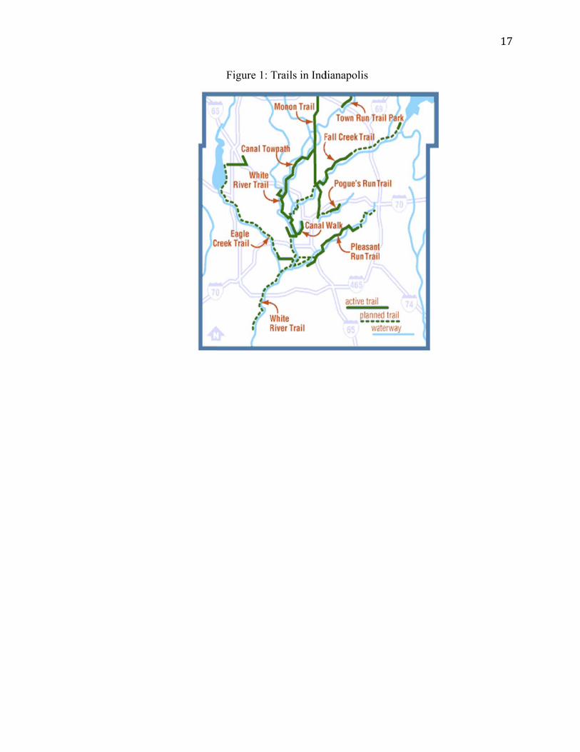
Figure 1: TTrails in Inddianapolis

17

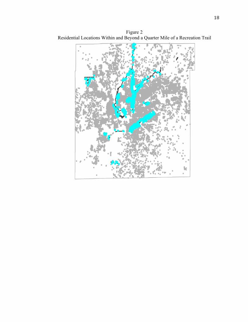
Resideential Locatiions Within Figure

and Beyond2

d a Quarter MMile of a Reccreation Trai

18

il

OpeninFigure

gDatesbyT3TrailSegmeent

19

HistogrammsofStandaObse

ardizedHeigervationsw

Figure

ght(haz)anwithz‐scores

4

ndWeight(satorAbov

waz)Scoresve3

safterDrop

20

pping

21

References [1] Anderson, M., and D. A. Matsa (2007), “Are Restaurants Really Supersizing America?”

Department of Agricultural Economics Working Paper. [2] Anderson, S. E., and R. C. Whitaker (2009), “Prevalence of Obesity Among US Preschool

Children in Different Racial and Ethnic Groups,” Archives of Pediatrics and Adolescent Medicine, 163(4), 344-348.

[3] Booth, K. M., M. M. Pinkston, and W. S. C. Poston (2005), “Obesity and the Built Environment,” Journal of the American Dietetic Association, 105, 110-117.

[4] Burdette, H. L., T. A. Wadden, and R. C. Whitaker (2006), “Neighborhood Safety, Collective Efficacy, and Obesity in Women with Young Children,” Obesity, 14, 518- 525.

[5] Burdette, H. L., and R. C. Whitaker (2004), “Neighborhood Playgrounds, Fast Food Restaurants, and Crime: Relationships to Overweight in Low- Income Preschool Children,” Preventive Medicine, 38, 57-63.

[6] Cawley, J., C. Meyerhoefer, and D. Newhouse (2007), “The Impact of State Physical Education Requirements on Youth Physical Activity and Overweight,” Health Economics, 16(12), 1287-1301.

[7] Centers for Disease Control and Prevention (1999), “Neighborhood Safety and the Prevalence of Physical Inactivity—Selected States 1996,” Retrieved from file:///Users/zhouxilin/Dropbox/GRA/trails%20paper%20modify/Neighborhood%20Safety%20and%20the%20Prevalence%20of%20Physical%20Inactivity%20‐‐%20Selected%20States,%201996.webarchive.

[8] Committee on Environmental Health (2009, June), “The Built Environment: Designing Communities to Promote Physical Activity in Children Organizational Principles to Guide and Define the Child Health Care System and/or Improve the Health of All Children,” Pediatrics 123(6), 1591-1598.

[9] Duncan, D. T., R. M. Johnson, B. E. Molnar, and D. Azrael (2009), “Association Between Neighborhood Safety and Overweight Status Among Urban Adolescents,” Retrieved from http://www.biomedcentral.com/1471‐2458/9/289/pre%20pub.

[10] Egger, G., and B. Swinburn (1997), “An ‘Ecological’ Approach to the Obesity Pandemic,” British Medical Journal, 315, 477- 480.

[11] Ewing, R., R. C. Brownson, and D. Berrigan (2006), “Relationship Between Urban Sprawl and Weight of United States Youth,” American Journal of Preventive Medicine, 31, 464–474.

[12] Ewing, R., T. Schmid, R. Killingworth, A. Zlot, and S. Raudenbush (2003), “Relationship Between Urban Sprawl and Physical Activity, Obesity, and Morbidity,” American Journal of Health Promotion, 18, 47- 57.

[13] Frank, L. D., M. A. Andresen, and T. L. Schmid (2004), “Obesity Relationship With Community Design, Physical Activity, and Time Spent in Cars,” American Journal of Preventive Medicine, 27, 87- 96.

[14] French, S. A., L. Harnack, and R. W. Jeffery (2000), “Fast Food Restaurant Use Among Women in the Pound of Prevention Study: Dietary, Behavioral and Demographic Correlates,” International Journal of Obesity, 24, 1353-1359.

[15] Giles-Corti, B., S. Macintyre, J. P. Clarkson, T. Pikora, and R. J. Donovan (2003), “Environmental and Lifestyle Factors Associated With Overweight and Obesity in Perth, Australia,” American Journal of Health Promotion, 18, 93- 102.

22

[16] Gordon-Larsen, P., M. C. Nelson, P. Page, and B. M. Popkin (2006), “Inequality in the Built Environment Underlies Key Health Disparities in Physical Activity and Obesity,” Pediatrics, 117, 417-424.

[17] Hannon, T. S., G. Rao and S. A. Arslanian (2005), “Childhood Obesity and Type 2 Diabetes Mellitus,” Pediatrics, Vol. 116, No. 2, 473-480.

[18] Hill, J. O., and J. C. Peters (1998), “Environmental Contributions to the Obesity Epidemic,” Science, 280, 1371- 1374.

[19] Hinkley, T., D. Crawford, J. Salmon, A. D. Okely, and K. Hesketh (2008), “Preschool Children and Physical Activity: A Review of Correlates,” American Journal of Preventive Medicine, 34, 435- 441.

[20] Jackson, R. J., and C. Kochtitzky (2002), “Creating a Healthy Environment: The Impact of the built Environment on Public Health,” Sprawl Watch Clearinghouse Monograph Series.

[21] Johnson, M. (2009, Oct. 7), “N.C. to Impose 'Fat Tax',” Retrieved from http://www.newsobserver.com/2009/10/07/129651/nc-to-impose-fat-tax.html.

[22] Kantor, J. (2007, January 8), “As Obesity Fight Hits Cafeteria, Many Fear a Note from School,” New York Times.

[23] King A. C., R. W. Jeffery, F. Fridinger, et al. (1995), “Environmental and Policy Approaches to Cardiovascular Disease Prevention Through Physical Activity: Issues and Opportunities,” Health Education and Behavior, Vol. 22, No. 4, 499-511.

[24] Kling, J. R., J. B. Liebman, L. F. Katz, and L. Sanbonmatsu (2004), “Moving to Opportunity and Tranquility: Neighborhood Effects on Adult Economic Self-Sufficiency and Health from a Randomized Housing Voucher Experiment,” Princeton IRS Working Paper No. 481.

[25] Li, F., K. J. Fisher, R. C. Brownson, and M. Bosworth (2005), “Multilevel Modeling of Built Environment Characteristics Related to Neighborhood Walking Activity in Older Adults,” Journal of Epidemiol and Cummunity Health, 59, 558- 564.

[26] Librett, J. J., M. M. Yore, and T. L. Schmid (2006), “Characteristics of Physical Activity Levels Among Trail Users in a U. S. National Sample,” American Journal of Preventive Medicine, 31, 399- 405.

[27] Limited Impact on Beverage Consumption Patterns in Maine High School Youth,” Journal of Nutrition and Education Behavior, Vol. 40, No. 6, 341-34

[28] Lindsey, G., and N. L. B. Doan (2002), “Urban Trails Heavily Used in Indiana,” Retrieved from http://www.policyinstitute.iu.edu/publicationDetail.aspx?PublicationID=59.

[29] Liu, G. C., C. Cunningham, S. M. Downs, D. G. Marrero, and N. Fineberg (2002), “A Spatial Analysis of Obesogenic Environments for Children,” Proceedings of the AMIA Symposium, 459 - 463.

[30] Lofholm, N. (2009, Oct. 10), “Heavy Infant in Grand Junction Denied Health Insurance,” Retrieved from http://www.denverpost.com/ci_13530098.

[31] Lumeng, J. C., D. Appugliese, H. J. Cabral, R. H. Bradley, and B. Zuckerman (2006), “Neighborhood Safety and Overweight Status in Children,” Archives of Pediatrics and Adolescent Medicine, 160, 25- 31.

[32] Margetts, B (2004), “WHO Global Strategy on Diet, Physical Activity and Health,” Editorial. Public Health Nutrition, 7, 361-363.

[33] Merom, D., A. Bauman, P. Vita, and G. Close (2003), “An Environmental Intervention to Promote Walking and Cycling- The Impact of a Newly Constructed Rail Trail in Western Sydney,” Preventive Medicine, 36, 235- 242.

23

[34] Millimet, D., R. Tchernis, and M. Hussain (2007), “School Nutrition Programs and the Incidence of Childhood Obesity,” CAEPR Working Paper No. 2007-014.

[35] Nelson, M. C., and P. Gordon-Larsen (2006), “Physical Activity and Sedentary Behavior Patterns Are Associated With Selected Adolescent Health Risk Behaviors,” Pediatrics, 117, 1281- 1692.

[36] Oliver, L. N., M. V. Hayes (2005), “Neighborhood Socio-Economic Status and the Prevalence of Overweight Canadian Children and Youth,” Canadian Journal of Public Health, 96, 415- 420.

[37] Ottensmann, J. R., G. Lindsey (2008), “A Use-Based Measure of Accessibility to Linear Features to Predict Urban Trail Use,” Journal of Transport and Land Use, 1, 41- 63.

[38] Papas, M. A., A. J. Alberg, R. Ewing, K. J. Helzlsouer, T. L. Gary, and A. C. Klassen (2007), “The Built Environment and Obesity,” Epidemiologic Reviews, 29, 129-143.

[39] Plantinga, A. J., and S. Bernell (2007), “The Association between Urban Sprawl and Obesity: Is It a Two-Way Street?” Journal of Regional Science, 47(5), 857-879.

[40] Poston, W. S. C., J. P. Foreyt (1999), “Obesity Is an Environmental Issue,” Atherosclerosis, 146, 201-209.

[41] Price, J., J. Murnan and B. Moore (2006), “Soft Drink Vending Machines in Schools: A Clear and Present Danger,” American Journal of Health Education, Vol. 37, No. 5, 306-314.

[42] Reynolds, K. D., J. Wolch, J. Byrne, C. Chou, G. Feng, S. Weaver, and M. Jerrett (2007), “Trail Characteristics As Correlates of Urban Trail Use,” American Journal of Health Promotion, 21, 335- 345.

[43] Romero, A. J., T. N. Robinson, H. C. Kraemer, S. J. Erickson, F. Haydel, F. Mendoza, and J. D. Killen (2001), “Are Perceived Neighborhood Hazards a Barrier to Physical Activity in Children?” Archives of Pediatrics and Adolescent Medicine, 155, 1143- 1148.

[44] Saelens, B. E., J. F. Sallis, L. D. Frank (2003), “Environmental Correlates of Walking and Cycling: Findings From the Transportation, Urban Design, and Planning Literatures,” Annals of Behavioral Medicine, 25, 80- 91.

[45] Salant, J. D. (2009, June 27),” Coca-Cola, Archer Daniels Fight to Kill Proposed Tax on Sodas,” Retrieved from http://www.bloomberg.com/apps/news?pid=newsarchive&sid=abiOPaVkntIU.

[46] Sallis, J. F., A. Bauman, and M. Pratt (1998), “Environmental and Policy Interventions to Promote Physical activity,” American Journal of Preventive Medicine, 15, 379-397.

[47] Sandell, C. (2009, Oct. 12), “Too Fat for Health Insurance? At Four Months?” Retrieved from http://abcnews.go.com/Health/fat-baby-health-insurance/story?id=8812582.

[48] Sandy, R., G. Liu, J. Ottensmann, R. Tchernis, J. Wilson, and O. T. Ford (2009), “Studying the Child Obesity Epidemic With Natural Experiments,” NBER Working Paper No. 14989.

[49] Sen, B., S. Mennemeyer, and L. C. Gary (2009), “The Relationship Between Neighborhood Quality and Obesity Among Children,” NBER Working Paper No. 14985.

[50] Stafford, M., A. Sacker, A. Ellaway, S. Cummins, D. Wiggins, and S. Macintyre (2008), “Neighborhood Effects on Health: A Structural Equation Modelling Approach,” Journal of Applied Social Science Studies, 128, 109- 120.

[51] Swinburn, B., G. Egger, and F. Raza (1999), “Dissecting Obesogenic Environments: The Development and Application of a Framework for Identifying and Prioritizing Environmental Interventions for Obesity,” Preventive Medicine, 29, 563-570.

[52] Trust for America’s Health (2009, July), “How Obesity Policies are Failing in America,” Retrieved from http://healthyamericans.org/reports/obesity2009/.

24

[53] Whatley Blum, J. E., A. Davee, C. M. Beaudoin, P. L. Jenkins, L. A. Kaley, and D. A. Wigand (2008), “Reduced Availability of Sugar-sweetened Beverages and Diet Soda Has a

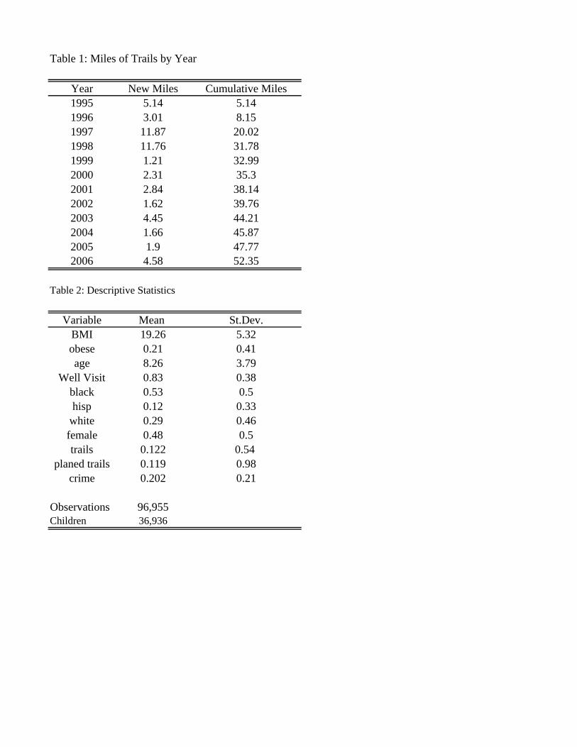
Table 1: Miles of Trails by Year

Year New Miles Cumulative Miles1995 5.14 5.141996 3.01 8.151997 11.87 20.021998 11.76 31.781999 1.21 32.992000 2.31 35.32001 2.84 38.142002 1.62 39.762003 4.45 44.212004 1.66 45.872005 1.9 47.772006 4.58 52.35

Table 2: Descriptive Statistics

Variable Mean St.Dev.BMI 19.26 5.32obese 0.21 0.41age 8.26 3.79

Well Visit 0.83 0.38black 0.53 0.5hisp 0.12 0.33

white 0.29 0.46female 0.48 0.5trails 0.122 0.54

planed trails 0.119 0.98crime 0.202 0.21

Observations 96,955Children 36,936

Table 3: FE Regressions on BMI

Full sample Age<8 Age>8

trails -0.144*** -0.0483 -0.200**(0.05) (0.04) (0.09)

crime 0.302** 0.324*** 0.247(0.13) (0.12) (0.25)

trails*crime 0.517** 0.224 0.754**(0.21) (0.16) (0.36)

Observations 96,955 50,836 46,119R-squared 0.327 0.063 0.155

Note: Robust standard errors in parentheses+ significant at 10%; * significant at 5%; ** significant at 1%All regressions include year and census tract fixed effectsControl variables: age, agesq, wc, black, hisp, white, female

Table 3.A: Effects of crime and trails in the full sample.

crime100 200 300 400 500 600 700 800

0 -0.144 -0.288 -0.432 -0.576 -0.72 -0.864 -1.008 -1.15210 -0.0621 -0.1544 -0.2467 -0.339 -0.4313 -0.5236 -0.6159 -0.708220 0.0198 -0.0208 -0.0614 -0.102 -0.1426 -0.1832 -0.2238 -0.264430 0.1017 0.1128 0.1239 0.135 0.1461 0.1572 0.1683 0.179440 0.1836 0.2464 0.3092 0.372 0.4348 0.4976 0.5604 0.623250 0.2655 0.38 0.4945 0.609 0.7235 0.838 0.9525 1.067

trails

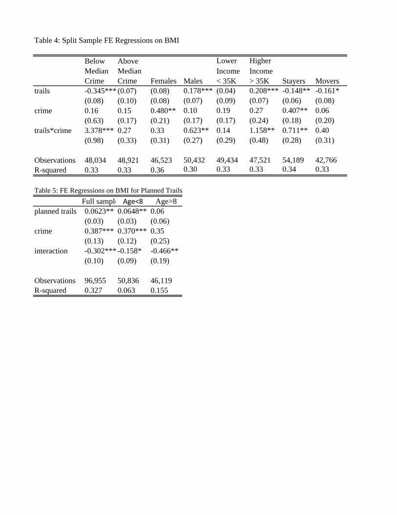
Table 4: Split Sample FE Regressions on BMI

Below Above Lower HigherMedian Median Income IncomeCrime Crime Males < 35K > 35K Stayers Movers

trails -0.345*** (0.07) (0.08) 0.178*** (0.04) 0.208*** -0.148** -0.161*(0.08) (0.10) (0.08) (0.07) (0.09) (0.07) (0.06) (0.08)

crime 0.16 0.15 0.480** 0.10 0.19 0.27 0.407** 0.06 (0.63) (0.17) (0.21) (0.17) (0.17) (0.24) (0.18) (0.20)

trails*crime 3.378*** 0.27 0.33 0.623** 0.14 1.158** 0.711** 0.40 (0.98) (0.33) (0.31) (0.27) (0.29) (0.48) (0.28) (0.31)

Observations 48,034 48,921 46,523 50,432 49,434 47,521 54,189 42,766 R-squared 0.33 0.33 0.36 0.30 0.33 0.33 0.34 0.33

Table 5: FE Regressions on BMI for Planned TrailsFull sample Age<8 Age>8

planned trails 0.0623** 0.0648** 0.06(0.03) (0.03) (0.06)

crime 0.387*** 0.370*** 0.35(0.13) (0.12) (0.25)

interaction -0.302*** -0.158* -0.466**(0.10) (0.09) (0.19)

Observations 96,955 50,836 46,119R-squared 0.327 0.063 0.155

Females

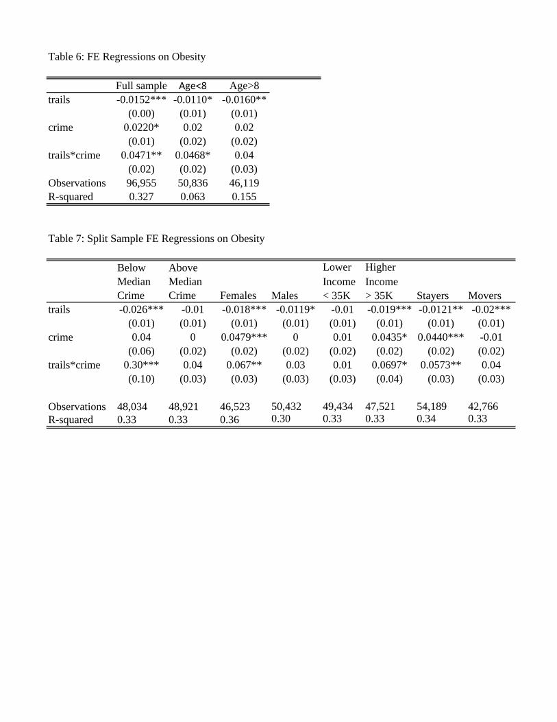
Table 6: FE Regressions on Obesity

Full sample Age<8 Age>8trails -0.0152*** -0.0110* -0.0160**

(0.00) (0.01) (0.01)crime 0.0220* 0.02 0.02

(0.01) (0.02) (0.02)trails*crime 0.0471** 0.0468* 0.04

(0.02) (0.02) (0.03)Observations 96,955 50,836 46,119R-squared 0.327 0.063 0.155

Table 7: Split Sample FE Regressions on Obesity

Below Above Lower HigherMedian Median Income IncomeCrime Crime Males < 35K > 35K Stayers Movers

trails -0.026*** -0.01 -0.018*** -0.0119* -0.01 -0.019*** -0.0121** -0.02***(0.01) (0.01) (0.01) (0.01) (0.01) (0.01) (0.01) (0.01)

crime 0.04 0 0.0479*** 0 0.01 0.0435* 0.0440*** -0.01(0.06) (0.02) (0.02) (0.02) (0.02) (0.02) (0.02) (0.02)

trails*crime 0.30*** 0.04 0.067** 0.03 0.01 0.0697* 0.0573** 0.04(0.10) (0.03) (0.03) (0.03) (0.03) (0.04) (0.03) (0.03)

Observations 48,034 48,921 46,523 50,432 49,434 47,521 54,189 42,766 R-squared 0.33 0.33 0.36 0.30 0.33 0.33 0.34 0.33

Females