Ocean Engineering 71 (2013) 103–112

Contents lists available at ScienceDirect

Ocean Engineering

0029-80

http://d

n Corr

E-m

journal homepage: www.elsevier.com/locate/oceaneng

Effects of climate change on stability of caisson breakwaters indifferent water depths

Kyung-Duck Suh a,n, Seung-Woo Kim b, Soyeon Kim c, Sehyeon Cheon b

a Department of Civil and Environmental Engineering & Engineering Research Institute, Seoul National University, 1 Gwanak-ro, Gwanak-gu,

Seoul 151-744, Republic of Koreab Department of Civil and Environmental Engineering, Seoul National University, 1 Gwanak-ro, Gwanak-gu, Seoul 151-744, Republic of Koreac Ocean Circulation and Climate Research Division, Korea Institute of Ocean Science & Technology, 787 Haean-ro, Sangnok-gu, Ansan-si,

Gyeonggi-do 426-744, Republic of Korea

a r t i c l e i n f o

Available online 19 March 2013

Keywords:

Artificial neural network

Caisson breakwater

Climate change

Sea-level rise

Water depth

Wave height

18/$ - see front matter & 2013 Elsevier Ltd. A

x.doi.org/10.1016/j.oceaneng.2013.02.017

esponding author. Tel.: þ82 2 880 8760; fax:

ail address: kdsuh@snu.ac.kr (K.-D. Suh).

a b s t r a c t

The effects of long-term sea-level rise and offshore wave-height increase due to climate change on the

stability of caisson breakwaters constructed in different water depths are analyzed by using a time-

dependent performance-based design method. An artificial neural network is combined with the wave

transformation model to reduce the computation time in the Monte Carlo simulation. The breakwater is

designed by the conventional safety-factor method, while its performance is evaluated by the expected

sliding distance. In general, the stability of the breakwater is reduced if the climate change effects are

included, but it shows different trends depending on water depth. Outside the surf zone, the effect of

sea-level rise decreases with increasing water depth, whereas that of wave-height increase increases

with water depth. Inside the surf zone, however, both effects decrease with decreasing water depth,

with greater effect of wave-height increase than sea-level rise. In the design of a caisson breakwater of

ordinary importance, it is not necessary to take into account the effect of sea-level rise, whereas the

effect of wave-height increase should be taken into account if the breakwater is constructed far outside

the surf zone. However, it should be noted that different results should be obtained if the breakwater

were designed based on the expected sliding distance.

& 2013 Elsevier Ltd. All rights reserved.

1. Introduction

Recent rapid climate change is drawing the attention of coastalengineers to its effect on the stability of existing coastal struc-tures. It is also important to take its effect into account in thedesign of new structures. However, since the current designstandards do not properly take into account the effects of climatechange, it is difficult to cope with possible structural risks in thefuture. Moreover, since the current deterministic design methoddoes not consider the uncertainties associated with the designvariables, it cannot cope with future climate change which alsoinvolves great uncertainty. In addition, the current method whichestimates the design variables based on the past environmentaldata is not suitable for taking into account the effect of rapidlychanging coastal environment in the design of coastal structuresof relatively long lifetime. Therefore, for properly taking intoaccount the effects of climate change in the design of coastalstructures, a probabilistic design method should be employed

ll rights reserved.

þ82 2 873 2684.

with accurately projected coastal environmental data for thefuture climate.

During the past several decades, many studies have beenconducted for the probabilistic design of vertical caisson break-waters. The papers presented in the books of Takayama (1994)and Kobayashi and Demirbilek (1995) describe the developmentof probabilistic design methods of vertical caisson breakwaters.Burcharth (1998) analyzed safety aspects mainly related tomonolithic caisson structures, and presented a partial safetyfactor system for overall stability failure modes. Shimosako andTakahashi (2000) proposed the performance-based designmethod, which was improved later by including new conceptsor design variables or by improving the calculation procedure(Goda and Takagi, 2000; Kim and Takayama, 2003; Hong et al.,2004; Esteban et al., 2007). Oumeraci et al. (2001) developedprobabilistic design tools based on levels II and III reliabilityanalyses and a partial safety factor system for verticalbreakwaters.

In this study, the performance-based design method isemployed, in which the expected sliding distance (ESD) duringthe lifetime of the breakwater is calculated. There are severalstudies for the performance-based design method that can takeinto account the effects of climate change. Okayasu and Sakai

2000 2020 2040 2060 2080 2100Year

0

0.2

0.4

0.6

0.8

1

1.2

Sea

leve

l (m

)

Scenario_A2meanmean + s.d.

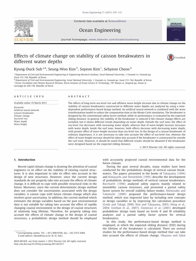
Fig. 1. Temporal variation of projected sea-level rise on Pacific Ocean side of Japan

by scenario A2.

0.3

0.4

0.5

ncy

Data: 10N (0.97, 0.02)

K.-D. Suh et al. / Ocean Engineering 71 (2013) 103–112104

(2006) proposed a method to calculate the optimal cross-sectionof a caisson considering sea-level rise. Takagi et al. (2011)evaluated the future stability of existing structures using theprojected increase of wind speed and wave height due to climatechange. Suh et al. (2012) proposed a method to incorporate suchclimate change effects as sea-level rise and wave-height increasein the performance-based design of a caisson breakwater.

The above-mentioned studies dealt with a breakwater con-structed in a particular water depth. Since a vertical caissonbreakwater can be constructed in various water depths inside oroutside the surf zone, it is necessary to investigate the climatechange effects on the stability of the structure depending on thewater depth. In this study, we analyze the climate change effectson fictitious breakwaters in various water depths near the EastBreakwater of the Port of Hitachinaka in Japan, which wasinvestigated by Suh et al. (2012). The breakwaters are designedby a deterministic method and the effects of climate change areanalyzed by the performance-based design method. The MonteCarlo simulation in the performance-based design methodrequires numerous calculations of wave transformation to calcu-late the waves at the location of the breakwater. An artificialneural network combined with a wave transformation model wasused to reduce the computation time.

The East Breakwater of the Port of Hitachinaka is 6-km long,and is parallel to the shoreline oriented in north–south direction.The bottom slope at the breakwater site is 1:100. The water depthat the breakwater site is 24.2 m below LWL, and the breakwater islocated approximately 2.6 km from the shoreline. The breakwateris a typical sloping-top caisson breakwater. The width of thecaisson is 22.0 m. The distance from LWL to the bottom of thecaisson is 18.5 m, and that to the top of the riprap foundation is17.0 m. The crest elevation above LWL is 9.5 m. The slope of thefront top of the caisson is 1:1. The seaward slope of the riprapfoundation is covered with armor blocks of 122.5 kN, and the rearberm is 10.0 m wide. See Suh et al. (2012) for details of thebreakwater cross-section.

0.9 0.92 0.94 0.96 0.98 1 1.02 1.04Hs_Exp/ Hs_Cal

0

0.1

0.2

Rel

ativ

e fre

que

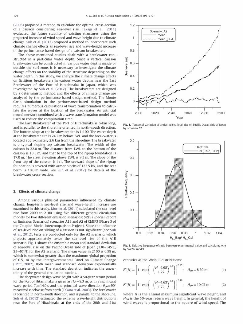
Fig. 2. Relative frequency of ratio between experimental value and calculated one

by SWAN model.

2. Effects of climate change

Among various physical parameters influenced by climatechange, long-term sea-level rise and wave-height increase areexamined in this study. Mori et al. (2011) calculated the sea-levelrise from 2000 to 2100 using five different general circulationmodels for two different emission scenarios: SRES (Special Reporton Emission Scenarios) scenarios A1B and A2 of CMIP3 (Phase 3 ofthe Coupled Model Intercomparison Project). Since the influenceof sea-level rise on sliding of a caisson is not significant (see Suhet al., 2012), tests are conducted only for the A2 scenario, whichprojects approximately twice the sea-level rise of the A1Bscenario. Fig. 1 shows the ensemble mean and standard deviationof sea-level rise on the Pacific Ocean side of Japan (130–1451E,25–401N) for the A2 scenario. The mean value in 2100 is 0.58 m,which is somewhat greater than the maximum global projectionof 0.51 m by the Intergovernmental Panel on Climate Change(IPCC, 2007). Both mean and standard deviation exponentiallyincrease with time. The standard deviation indicates the uncer-tainty of the general circulation models.

The deepwater design wave height with a 50-year return periodfor the Port of Hitachinaka is given as Hs0¼8.3 m, with a significantwave period Ts¼14.0 s and the principal wave direction yp0¼901measured clockwise from north (Takata et al., 2003). The breakwateris oriented in north–south direction, and is parallel to the shoreline.Suh et al. (2012) estimated the extreme wave-height distributionsnear the Port of Hitachinaka at the ends of the 20th and 21st

centuries as the Weibull distributions:

FnðHÞ ¼ 1�exp �

H�4:65

1:27

� �1:0( )" #0:35

; H50 ¼ 8:30 m ð1Þ

FnðHÞ ¼ 1�exp �

H�4:63

1:72

� �1:0( )" #0:46

; H50 ¼ 10:02 m ð2Þ

where H is the annual maximum significant wave height, andH50 is the 50-year return wave height. In general, the height ofwind waves is proportional to the square of wind speed. The

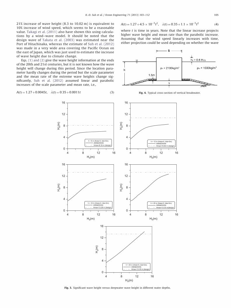
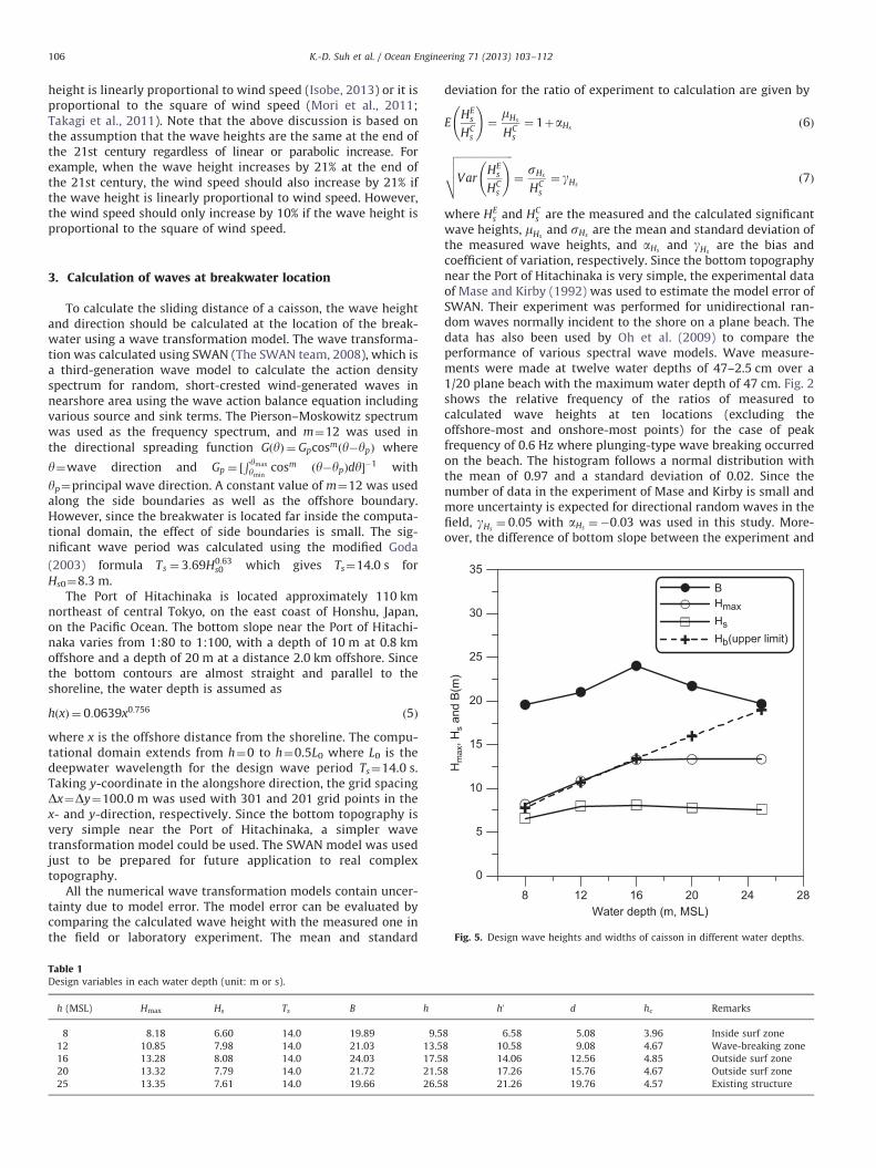
Fig. 4. Typical cross-section of vertical breakwater.

K.-D. Suh et al. / Ocean Engineering 71 (2013) 103–112 105

21% increase of wave height (8.3 to 10.02 m) is equivalent to10% increase of wind speed, which seems to be a reasonablevalue. Takagi et al. (2011) also have shown this using calcula-tions by a wind–wave model. It should be noted that thedesign wave of Takata et al. (2003) was estimated near thePort of Hitachinaka, whereas the estimate of Suh et al. (2012)was made in a very wide area covering the Pacific Ocean onthe east of Japan, which was just used to estimate the increaseof wave height due to climate change.

Eqs. (1) and (2) give the wave height information at the endsof the 20th and 21st centuries, but it is not known how the waveheight will change during this period. Since the location para-meter hardly changes during the period but the scale parameterand the mean rate of the extreme wave heights change sig-nificantly, Suh et al. (2012) assumed linear and parabolicincreases of the scale parameter and mean rate, i.e.,

AðtÞ ¼ 1:27þ0:0045t, lðtÞ ¼ 0:35þ0:0011t ð3Þ

0

4

8

12

16

Hs(

m)

H0(m)

H0(m)

0

4

8

12

16

Hs(

m)

4 8 12 16

4 8 12 16

40

4

8

12

16

Hs(m

)

Fig. 3. Significant wave height versus deepwat

AðtÞ ¼ 1:27þ4:5� 10�5t2, lðtÞ ¼ 0:35þ1:1� 10�5t2 ð4Þ

where t is time in years. Note that the linear increase projectshigher wave height and mean rate than the parabolic increase.Assuming that the wind speed linearly increases with time,either projection could be used depending on whether the wave

Hs(

m)

Hs(

m)

H0(m)

H0(m)

0

4

8

12

16

4 8 12 16

4 8 12 160

4

8

12

16

8 12 16H0(m)

er wave height in different water depths.

K.-D. Suh et al. / Ocean Engineering 71 (2013) 103–112106

height is linearly proportional to wind speed (Isobe, 2013) or it isproportional to the square of wind speed (Mori et al., 2011;Takagi et al., 2011). Note that the above discussion is based onthe assumption that the wave heights are the same at the end ofthe 21st century regardless of linear or parabolic increase. Forexample, when the wave height increases by 21% at the end ofthe 21st century, the wind speed should also increase by 21% ifthe wave height is linearly proportional to wind speed. However,the wind speed should only increase by 10% if the wave height isproportional to the square of wind speed.

8 12 16 20 24 28Water depth (m, MSL)

0

5

10

15

20

25

30

35

Hm

ax, H

s and

B(m

)

BHmaxHsHb(upper limit)

Fig. 5. Design wave heights and widths of caisson in different water depths.

3. Calculation of waves at breakwater location

To calculate the sliding distance of a caisson, the wave heightand direction should be calculated at the location of the break-water using a wave transformation model. The wave transforma-tion was calculated using SWAN (The SWAN team, 2008), which isa third-generation wave model to calculate the action densityspectrum for random, short-crested wind-generated waves innearshore area using the wave action balance equation includingvarious source and sink terms. The Pierson–Moskowitz spectrumwas used as the frequency spectrum, and m¼12 was used in

the directional spreading function GðyÞ ¼ Gpcosmðy�ypÞ where

y¼wave direction and Gp ¼ ½R ymax

ymincosm ðy�ypÞdy��1 with

yp¼principal wave direction. A constant value of m¼12 was usedalong the side boundaries as well as the offshore boundary.However, since the breakwater is located far inside the computa-tional domain, the effect of side boundaries is small. The sig-nificant wave period was calculated using the modified Goda

(2003) formula Ts ¼ 3:69H0:63s0 which gives Ts¼14.0 s for

Hs0¼8.3 m.The Port of Hitachinaka is located approximately 110 km

northeast of central Tokyo, on the east coast of Honshu, Japan,on the Pacific Ocean. The bottom slope near the Port of Hitachi-naka varies from 1:80 to 1:100, with a depth of 10 m at 0.8 kmoffshore and a depth of 20 m at a distance 2.0 km offshore. Sincethe bottom contours are almost straight and parallel to theshoreline, the water depth is assumed as

hðxÞ ¼ 0:0639x0:756 ð5Þ

where x is the offshore distance from the shoreline. The compu-tational domain extends from h¼0 to h¼0.5L0 where L0 is thedeepwater wavelength for the design wave period Ts¼14.0 s.Taking y-coordinate in the alongshore direction, the grid spacingDx¼Dy¼100.0 m was used with 301 and 201 grid points in thex- and y-direction, respectively. Since the bottom topography isvery simple near the Port of Hitachinaka, a simpler wavetransformation model could be used. The SWAN model was usedjust to be prepared for future application to real complextopography.

All the numerical wave transformation models contain uncer-tainty due to model error. The model error can be evaluated bycomparing the calculated wave height with the measured one inthe field or laboratory experiment. The mean and standard

Table 1Design variables in each water depth (unit: m or s).

h (MSL) Hmax Hs Ts B h

8 8.18 6.60 14.0 19.89 9.5

12 10.85 7.98 14.0 21.03 13.5

16 13.28 8.08 14.0 24.03 17.5

20 13.32 7.79 14.0 21.72 21.5

25 13.35 7.61 14.0 19.66 26.5

deviation for the ratio of experiment to calculation are given by

EHE

s

HCs

!¼mHs

HCs

¼ 1þaHsð6Þ

ffiffiffiffiffiffiffiffiffiffiffiffiffiffiffiffiffiffiffiffiffiffiVar

HEs

HCs

!vuut ¼sHs

HCs

¼ gHsð7Þ

where HEs and HC

s are the measured and the calculated significantwave heights, mHs

and sHsare the mean and standard deviation of

the measured wave heights, and aHsand gHs

are the bias andcoefficient of variation, respectively. Since the bottom topographynear the Port of Hitachinaka is very simple, the experimental dataof Mase and Kirby (1992) was used to estimate the model error ofSWAN. Their experiment was performed for unidirectional ran-dom waves normally incident to the shore on a plane beach. Thedata has also been used by Oh et al. (2009) to compare theperformance of various spectral wave models. Wave measure-ments were made at twelve water depths of 47–2.5 cm over a1/20 plane beach with the maximum water depth of 47 cm. Fig. 2shows the relative frequency of the ratios of measured tocalculated wave heights at ten locations (excluding theoffshore-most and onshore-most points) for the case of peakfrequency of 0.6 Hz where plunging-type wave breaking occurredon the beach. The histogram follows a normal distribution withthe mean of 0.97 and a standard deviation of 0.02. Since thenumber of data in the experiment of Mase and Kirby is small andmore uncertainty is expected for directional random waves in thefield, gHs

¼ 0:05 with aHs¼�0:03 was used in this study. More-

over, the difference of bottom slope between the experiment and

h0 d hc Remarks

8 6.58 5.08 3.96 Inside surf zone

8 10.58 9.08 4.67 Wave-breaking zone

8 14.06 12.56 4.85 Outside surf zone

8 17.26 15.76 4.67 Outside surf zone

8 21.26 19.76 4.57 Existing structure

Tide level and

wave transformation

Rayleigh - distributed wave

heights and breaking

Sliding model

Summation for one storm

foronestorm

Summation until t year

forservicelifetime(TL)

50,000simulations

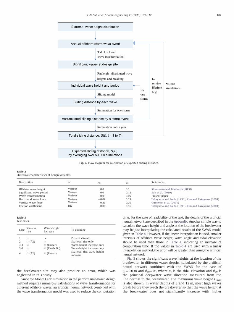
Fig. 6. Flow diagram for calculation of expected sliding distance.

Table 2Statistical characteristics of design variables.

Description Xi aXigXi

References

Offshore wave height Various 0.0 0.1 Shimosako and Takahashi (2000)

Significant wave period Various 0.0 0.12 Suh et al. (2010)

Wave transformation Various �0.03 0.05 Present paper

Horizontal wave force Various �0.09 0.19 Takayama and Ikeda (1993), Kim and Takayama (2003)

Vertical wave force Various �0.23 0.20 Oumeraci et al. (2001)

Friction coefficient 0.6 0.06 0.16 Takayama and Ikeda (1993), Kim and Takayama (2003)

Table 3Test cases.

CaseSea-level

rise

Wave-height

increaseTo examine

1 � � Present climate

2 J (A2) � Sea-level rise only

3-1 � J (Linear) Wave-height increase only

3-2 � J (Parabolic) Wave-height increase only

4 J (A2) J (Linear)Sea-level rise, wave-height

increase

K.-D. Suh et al. / Ocean Engineering 71 (2013) 103–112 107

the breakwater site may also produce an error, which wasneglected in this study.

Since the Monte Carlo simulation in the performance-based designmethod requires numerous calculations of wave transformation fordifferent offshore waves, an artificial neural network combined withthe wave transformation model was used to reduce the computation

time. For the sake of readability of the text, the details of the artificialneural network are described in the Appendix. Another simple way tocalculate the wave height and angle at the location of the breakwatermay be just interpolating the calculated results of the SWAN modelgiven in Table 4. However, if the linear interpolation is used, smallerintervals of offshore wave height, wave angle and tidal elevationshould be used than those in Table 4, indicating an increase ofcomputation time. If the values in Table 4 are used with a linearinterpolation method, the error will be greater than using the artificialneural network.

Fig. 3 shows the significant wave heights, at the location of thebreakwater in different water depths, calculated by the artificialneural network combined with the SWAN for the case ofZt¼0.0 m and yp0¼01, where Zt is the tidal elevation and yp0 isthe principal deepwater wave direction measured from theline normal to the breakwater. The maximum wave height Hmax

is also shown. In water depths of 8 and 12 m, most high wavesbreak before they reach the breakwater so that the wave height atthe breakwater does not significantly increase with higher

K.-D. Suh et al. / Ocean Engineering 71 (2013) 103–112108

deepwater wave heights. In water depths greater than 20 m,however, little wave breaking occurs so that the significant waveheight at the breakwater increases with the higher deepwaterwave heights.

0.8

1

w/o cce

4. Breakwater design

To examine how the climate change effects change with waterdepth, fictitious breakwaters were designed in various water depthsnear the Port of Hitachinaka in Japan. Using the empirical relationshipbetween the breaking wave height and water depth in ShoreProtection Manual (U.S. Army Coastal Engineering Research Center,1977), the breaking depth for the design waves was calculated to bebetween 10.7 and 13.4 m using mean sea level (MSL) condition. Thebreakwaters were designed in five different water depths: 8 m (insidethe surf zone), 12 m (wave-breaking zone), and 16, 20, and 25 m(outside the surf zone) in water under MSL. The greatest water depth(i.e. 25 m) is the actual water depth of the East Breakwater of the Portof Hitachinaka. Fig. 4 shows the cross-section of the breakwater, inwhich B is the caisson width, hc¼0.6Hs is the crest elevation,tr¼max{0.2 h, 3.0 m} is the thickness of the rubble mound founda-tion, and rc and rw are the densities of the upright section and seawater, respectively. The height of foot-protection blocks and the bermwidth of rubble foundation were 1.5 m and 8.0 m, respectively,regardless of water depth. The safety factor against caisson slidingwas set at 1.2 as in current design standards. Table 1 shows thedesign variables in each water depth, where h, h0, and d indicate thewater depths from the design water level to seabed, bottom ofcaisson, and front berm of rubble mound, respectively. The designwater level at the Port of Hitachinaka is 1.58 m above MSL, which isthe sum of tidal amplitude (0.75 m) and storm surge height (0.83 m).Even though the bottom slope is calculated to be between 0.007 and0.01 by Eq. (5), a constant value of 0.01 was used in all water depthsfor simplicity.

Fig. 5 shows the design significant wave heights, maximumwave heights and caisson widths at different water depths in thepresent climate condition. The limiting breaker height of Goda(1974) is also plotted. The caisson width increases with waterdepth up to the depth of 16 m, after which it decreases. On theother hand, both significant and maximum wave heights do notchange significantly in water depths greater than 16 m. It isexpected that the ESD during the lifetime of the breakwater willbe small in water depths smaller than 16 m where the maximumwave height is limited by wave breaking. However, it will becomelarger in greater water depths where the maximum wave heightis not limited by wave breaking.

8 12 16 20 24 28Water depth (m)

0

0.2

0.4

0.6

SE(m

)

Fig. 7. Expected sliding distance versus water depth without consideration of

climate change effects.

5. Performance evaluation

The performance of the breakwaters designed by the determi-nistic method is evaluated by calculating the ESD using theperformance-based design method. The computational procedureto calculate the ESD and the mathematical model to calculate thesliding distance can be found in many papers (Shimosako andTakahashi, 2000; Goda and Takagi, 2000; Kim and Takayama,2003; Hong et al., 2004), so the details are not repeated in thispaper. Only the flow chart for calculation of the ESD is shown inFig. 6. The ESD is calculated with Monte Carlo simulationsto account for uncertainties in various design variables. In thisstudy, the time-dependent performance-based design method(Suh et al., 2012) is used, which expresses the mean sea leveland wave climate as functions of time to account for the effects ofclimate change so that the time-dependent ESD SE(t) is calculatedover the service life of the breakwater [0,TL].

The uncertainty of a design variable whose characteristic valueis X is represented by

mX ¼ ð1þaXÞX; sX ¼ gXX ð8Þ

The statistical characteristics of the design variables are givenin Table 2, along with the corresponding references. The variationof water level due to tide and storm surge is also included in thesimulations as described in Fig. 6 and the Appendix. With a tidalrange of DZ¼1.5 m, the tide level Zt was simply assumed to varysinusoidally between LWL (Zt¼0) and HWL (Zt¼DZ). For simpli-city, the effect of storm surge was taken into account by adding10% of the deepwater significant wave height to the tide level(Shimosako and Takahashi, 1998; Kim and Takayama, 2003).Since the increase of wave height due to climate change is takeninto account, the influence of climate change on storm surge isalso taken into account indirectly.

In general, caisson sliding occurs when the structure enduressevere storm waves. The annual maximum wave height isconsidered sufficient for the design calculation. The annual max-imum offshore significant wave height is randomly sampled fromthe extreme wave height distributions given by Eqs. (1) and (2).The number of waves during a storm was assumed to be 1000,which corresponds to approximately 3.2 h for the design wavewith Ts¼14.0 s. These assumptions may not be appropriate in realapplications. A better approach would be to treat these para-meters as probabilistic ones. The number of Monte Carlo simula-tions was 50,000, which consists of 10,000 simulations with fivedifferent initial random seeds.

Computations were conducted for a series of four test cases(see Table 3). Case 1 is for the present climate with neither sea-level rise nor wave-height increase. Case 2 examines the influenceof sea-level rise (A2 scenario). Cases 3-1 and 3-2 respectivelyexamine the linear and parabolic increases of wave height. Case4 examines both sea-level rise and linear increase of wave height.It is assumed that the breakwater was constructed in 2000, andthe computations were made for t¼0–50 years, from 2000to 2050.

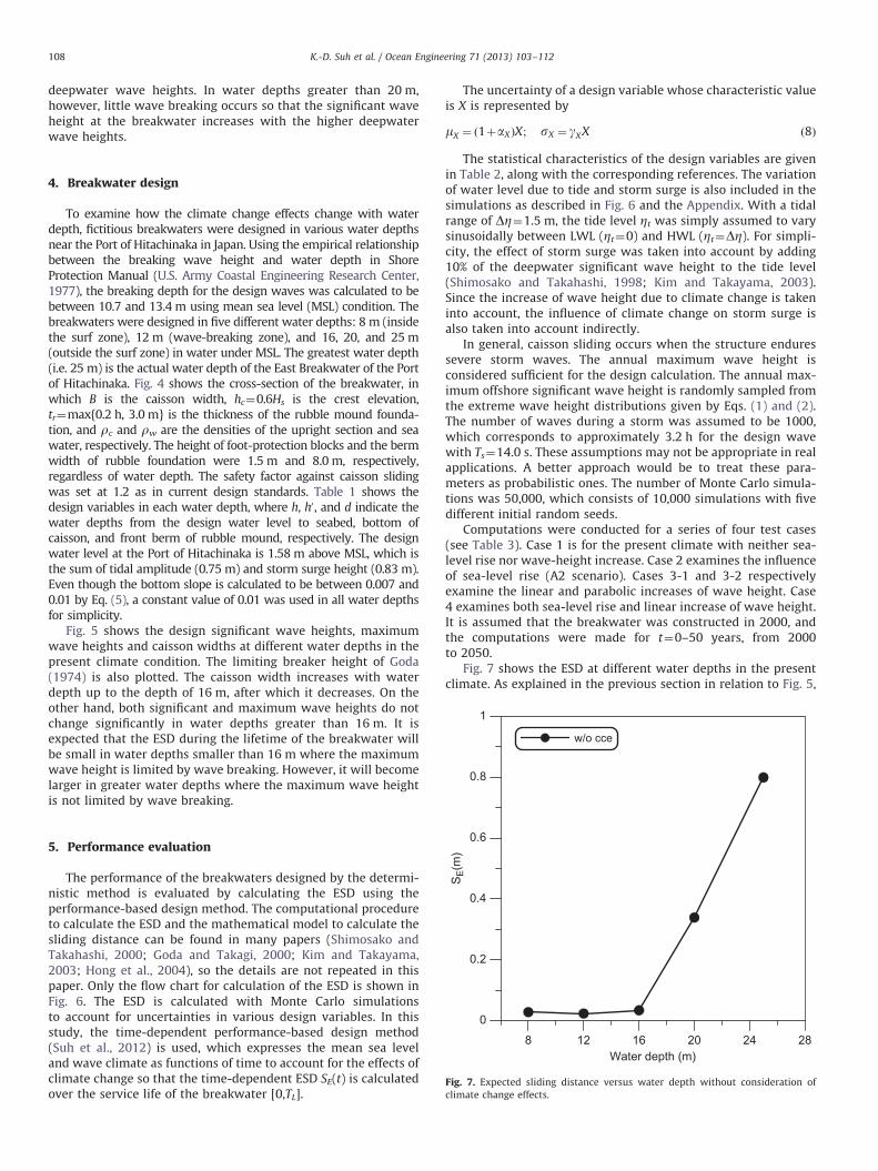
Fig. 7 shows the ESD at different water depths in the presentclimate. As explained in the previous section in relation to Fig. 5,

K.-D. Suh et al. / Ocean Engineering 71 (2013) 103–112 109

the ESD is very small up to the water depth of 16 m, after whichthe ESD rapidly increases with water depth. Considering that theallowable ESD of the structure of ordinary importance is 0.3 m(Takahashi et al., 2001), Fig. 7 shows that the deterministicmethod severely over-designs the caisson width in water depthsup to 16 m, while under-designing in deeper waters. If theperformance-based design method were used, the caisson widthgiving approximately 30 cm of ESD could be calculated in eachwater depth.

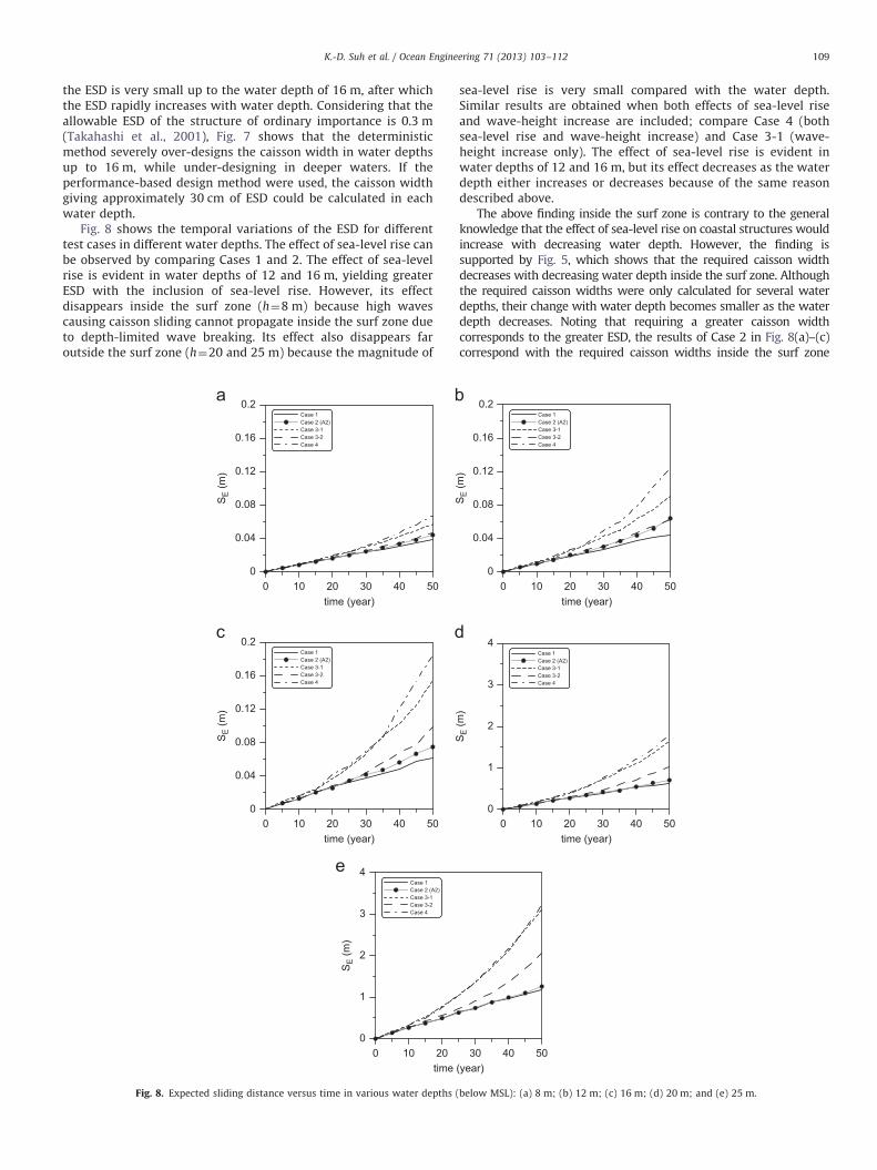
Fig. 8 shows the temporal variations of the ESD for differenttest cases in different water depths. The effect of sea-level rise canbe observed by comparing Cases 1 and 2. The effect of sea-levelrise is evident in water depths of 12 and 16 m, yielding greaterESD with the inclusion of sea-level rise. However, its effectdisappears inside the surf zone (h¼8 m) because high wavescausing caisson sliding cannot propagate inside the surf zone dueto depth-limited wave breaking. Its effect also disappears faroutside the surf zone (h¼20 and 25 m) because the magnitude of

time (year)

0

0.04

0.08

0.12

0.16

0.2

SE (m

)S

E (m

)

SE (m

)

time (year)

0

0.04

0.08

0.12

0.16

0.2

0 10 20 30 40 50

0 10 20 30 40 50

0 10 20time

0

1

2

3

4

Fig. 8. Expected sliding distance versus time in various water depths (

sea-level rise is very small compared with the water depth.Similar results are obtained when both effects of sea-level riseand wave-height increase are included; compare Case 4 (bothsea-level rise and wave-height increase) and Case 3-1 (wave-height increase only). The effect of sea-level rise is evident inwater depths of 12 and 16 m, but its effect decreases as the waterdepth either increases or decreases because of the same reasondescribed above.

The above finding inside the surf zone is contrary to the generalknowledge that the effect of sea-level rise on coastal structures wouldincrease with decreasing water depth. However, the finding issupported by Fig. 5, which shows that the required caisson widthdecreases with decreasing water depth inside the surf zone. Althoughthe required caisson widths were only calculated for several waterdepths, their change with water depth becomes smaller as the waterdepth decreases. Noting that requiring a greater caisson widthcorresponds to the greater ESD, the results of Case 2 in Fig. 8(a)–(c)correspond with the required caisson widths inside the surf zone

SE (m

)S

E (m

)

time (year)

0

0.04

0.08

0.12

0.16

0.2

time (year)

0

1

2

3

4

0 10 20 30 40 50

0 10 20 30 40 50

30 40 50(year)

below MSL): (a) 8 m; (b) 12 m; (c) 16 m; (d) 20 m; and (e) 25 m.

K.-D. Suh et al. / Ocean Engineering 71 (2013) 103–112110

shown in Fig. 5. Goda (2010; Section 4.3.2) showed that the requiredcaisson width even increases with decreasing water depth far insidethe surf zone, indicating that a smaller caisson width could berequired (or a smaller ESD could be calculated) as the water depthincreases by the sea-level rise. However, it is rare to build a caissonbreakwater far inside the surf zone.

On the other hand, the effect of wave-height increase (Cases 3-1 and 3-2) decreases with decreasing water depth because higherwaves break offshore before they reach the breakwater in smallwater depth. Inside the surf zone (h¼8 and 12 m), the effect ofparabolic increase of wave height is almost the same as that ofsea-level rise. In all water depths, the increase of ESD due to linearwave-height increase is almost twice that due to parabolicincrease.

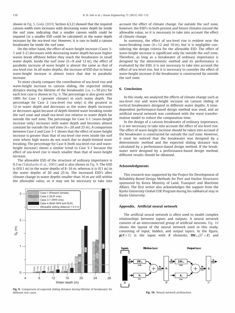
To more clearly compare the contribution of sea-level rise andwave-height increase to caisson sliding, the expected slidingdistance during the lifetime of the breakwater (i.e. t¼50 yrs) foreach test case is shown in Fig. 9. The percentage is also given with100% for Case 1 (present climate) in each water depth. Thepercentage for Case 2 (sea-level rise only) is the greatest in12-m water depth and decreases as the water depth increasesor decreases again because of depth-limited wave breaking insidethe surf zone and small sea-level rise relative to water depth faroutside the surf zone. The percentage for Case 3-1 (wave-heightincrease only) increases with water depth and becomes almostconstant far outside the surf zone (h¼20 and 25 m). A comparisonbetween Case 2 and Case 3-1 shows that the effect of wave-heightincrease is greater than that of sea-level rise even inside the surfzone where high waves do not reach due to depth-limited wavebreaking. The percentage for Case 4 (both sea-level rise and wave-height increase) shows a similar trend to Case 3-1 because theeffect of sea-level rise is much smaller than that of wave-heightincrease.

The allowable ESD of the structure of ordinary importance is0.3 m (Takahashi et al., 2001) and is also shown in Fig. 9. The ESDis O(0.1 m) in the water depths of 8–16 m, whereas it is O(1 m) inthe water depths of 20 and 25 m. The increased ESD’s afterclimate change in water depths smaller than 16 m are still withinthe allowable value, so it may not be necessary to take into

4 8 12 16 20 24 28Water depth (m)

0

1

2

3

SE (m

)

Case 1 (Present climate)Case 2 (SLR only)Case 3-1 (WHI only)Case 4 (Both WHI and SLR)Allowable sliding distance = 0.3 m

100%

114%

147%

173%

100%

147%

206% 28

5%

100%

122% 25

2%30

2%

100% 11

3%26

3%28

8%

100% 10

6%26

2%27

1%

Fig. 9. Comparison of expected sliding distance during lifetime of breakwater for

different test cases.

account the effect of climate change. Far outside the surf zone,however, the ESD’s in both present and future climates exceed theallowable value, so it is necessary to take into account the effectof climate change.

In summary, the effect of sea-level rise is evident near thewave-breaking zone (h¼12 and 16 m), but it is negligible con-sidering the design criteria for the allowable ESD. The effect ofwave-height increase is significant only far outside the surf zone.Therefore, as long as a breakwater of ordinary importance isdesigned by the deterministic method and its performance isevaluated by the ESD, it is not necessary to take into account theeffect of sea-level rise, but it is necessary to consider the effect ofwave-height increase if the breakwater is constructed far outsidethe surf zone.

6. Conclusion

In this study, we analyzed the effects of climate change such assea-level rise and wave-height increase on caisson sliding ofvertical breakwaters designed in different water depths. A time-dependent performance-based design method was used, and anartificial neural network was combined with the wave transfor-mation model to reduce the computation time.

In the design of a caisson breakwater of ordinary importance,it is not necessary to take into account the effect of sea-level rise.The effect of wave-height increase should be taken into account ifthe breakwater is constructed far outside the surf zone. However,it must be noticed that the breakwater was designed by adeterministic method and the expected sliding distance wascalculated by a performance-based design method. If the break-water were designed by a performance-based design method,different results should be obtained.

Acknowledgments

This research was supported by the Project for Development ofReliability-Based Design Methods for Port and Harbor Structuressponsored by Korea Ministry of Land, Transport and MaritimeAffairs. The first writer also acknowledges the support from theKyoto University Global COE Program during his sabbatical stay inKyoto University.

Appendix. Artificial neural network

The artificial neural network is often used to model complexrelationships between inputs and outputs. A neural networkconsists of an interconnected group of artificial neurons. Fig. 10shows the layout of the neural network used in this study,consisting of input, hidden, and output layers. In the figure,p(R�1) is the input with R elements, IW1,1(S1

�R) and

Fig. 10. Neural network architecture.

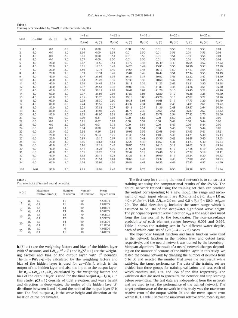
Table 4Training sets calculated by SWAN in different water depths.

Case Hs0 (m) yp0 (1) Zt (m)

h¼8 m h¼12 m h¼16 m h¼20 m h¼25 m

Hs (m) yp (1) Hs (m) yp (1) Hs (m) yp (1) Hs (m) yp (1) Hs (m) yp (1)

1 4.0 0.0 0.0 3.73 0.00 3.55 0.00 3.50 0.01 3.50 0.01 3.53 0.01

2 4.0 0.0 1.0 3.66 0.00 3.53 0.01 3.50 0.01 3.51 0.01 3.53 0.01

3 4.0 0.0 2.0 3.61 0.00 3.51 0.01 3.50 0.01 3.51 0.01 3.54 0.01

4 4.0 0.0 3.0 3.57 0.00 3.50 0.01 3.50 0.01 3.51 0.01 3.55 0.01

5 4.0 20.0 0.0 3.67 11.50 3.51 13.72 3.48 15.49 3.49 16.65 3.52 17.72

6 4.0 20.0 1.0 3.61 12.15 3.49 14.20 3.48 15.83 3.50 16.90 3.53 17.89

7 4.0 20.0 2.0 3.56 12.76 3.49 14.64 3.48 16.13 3.50 17.13 3.54 18.04

8 4.0 20.0 3.0 3.53 13.31 3.48 15.04 3.48 16.42 3.51 17.34 3.55 18.19

9 4.0 40.0 0.0 3.47 21.95 3.36 26.34 3.37 29.92 3.41 32.32 3.47 34.59

10 4.0 40.0 1.0 3.43 23.23 3.35 27.30 3.38 30.60 3.42 32.83 3.48 34.95

11 4.0 40.0 2.0 3.39 24.42 3.35 28.18 3.39 31.23 3.43 33.31 3.50 35.28

12 4.0 40.0 3.0 3.37 25.54 3.36 29.00 3.40 31.83 3.45 33.76 3.51 35.60

13 4.0 60.0 0.0 3.00 30.12 2.95 36.47 3.02 41.76 3.10 45.45 3.22 49.10

14 4.0 60.0 1.0 2.97 31.96 2.96 37.87 3.04 42.80 3.12 46.26 3.25 49.70

15 4.0 60.0 2.0 2.95 33.70 2.98 39.18 3.06 43.78 3.15 47.02 3.27 50.26

16 4.0 60.0 3.0 2.95 35.30 2.99 40.38 3.08 44.68 3.17 47.73 3.29 50.79

17 4.0 80.0 0.0 2.24 35.52 2.25 43.37 2.34 50.03 2.45 54.81 2.61 59.72

18 4.0 80.0 1.0 2.23 37.81 2.27 45.11 2.37 51.36 2.48 55.87 2.64 60.54

19 4.0 80.0 2.0 2.23 39.93 2.29 46.73 2.39 52.61 2.51 56.87 2.67 61.32

20 4.0 80.0 3.0 2.23 41.90 2.31 48.25 2.42 53.78 2.54 57.82 2.70 62.06

21 6.0 0.0 0.0 5.39 0.21 5.92 0.00 5.62 0.00 5.50 0.00 5.45 0.00

22 6.0 0.0 1.0 5.71 0.07 5.83 0.00 5.57 0.00 5.48 0.00 5.44 0.00

23 6.0 0.0 2.0 5.90 0.01 5.75 0.00 5.54 0.00 5.47 0.00 5.44 0.00

24 6.0 0.0 3.0 5.94 0.00 5.68 0.00 5.51 0.00 5.46 0.00 5.44 0.00

25 6.0 20.0 0.0 5.34 9.16 5.84 10.99 5.55 12.68 5.44 13.93 5.41 15.21

26 6.0 20.0 1.0 5.65 9.64 5.75 11.43 5.51 13.03 5.43 14.21 5.40 15.43

27 6.0 20.0 2.0 5.83 10.15 5.67 11.84 5.48 13.36 5.42 14.48 5.40 15.63

28 6.0 20.0 3.0 5.86 10.63 5.61 12.23 5.46 13.67 5.41 14.73 5.40 15.83

29 6.0 40.0 0.0 5.16 17.19 5.45 20.85 5.24 24.13 5.17 26.62 5.18 29.24

30 6.0 40.0 1.0 5.41 18.23 5.39 21.68 5.21 24.81 5.17 27.18 5.19 29.68

31 6.0 40.0 2.0 5.51 19.23 5.33 22.47 5.19 25.46 5.17 27.72 5.19 30.11

32 6.0 40.0 3.0 5.52 20.14 5.28 23.23 5.18 26.09 5.17 28.24 5.20 30.52

33 6.0 60.0 0.0 4.69 23.54 4.61 28.66 4.48 33.37 4.48 37.00 4.55 40.93

34 6.0 60.0 1.0 4.74 25.04 4.56 29.84 4.47 34.35 4.49 37.83 4.57 41.60

^ ^ ^ ^ ^ ^ ^ ^ ^ ^ ^ ^ ^ ^120 14.0 80.0 3.0 7.85 19.99 9.45 22.85 9.75 25.90 9.50 28.38 9.20 31.34

Table 5Characteristics of trained neural networks.

h (m)Maximum

relative error (%)

Number

of neuron

Number

of iteration

Mean

square error

8Hs 1.0 11 60 5.55E04

yp 0.1 11 10 1.84E03

12Hs 1.8 13 80 6.01E04

yp 0.1 13 30 9.37E03

16Hs 1.6 12 70 4.90E03

yp 0.1 12 20 1.35E03

20Hs 1.9 14 90 9.50E04

yp 0.1 11 10 7.17E04

25Hs 1.0 6 10 4.04E04

yp 0.1 11 10 3.64E03

K.-D. Suh et al. / Ocean Engineering 71 (2013) 103–112 111

b1(S1�1) are the weighting factors and bias of the hidden layer

with S1 neurons, and LW2,1(S2� S1) and b2(S2

�1) are the weight-ing factors and bias of the output layer with S2 neurons.The n1 ¼ IW1,1dpþb1 calculated by the weighting factors andbias of the hidden layer is used for a1¼f1(n1), which is theoutput of the hidden layer and also the input to the output layer.The n2 ¼ LW2,1da1þb2 calculated by the weighting factors andbias of the output layer is used for the final output a2¼f2(n2). Inthis study, p(3�1) consists of tidal elevation, and wave heightand direction in deep water, the nodes of the hidden layer S1

distribute between 6 and 14, and the node of the output layer S2 isone. The final output a2 is the wave height and direction at thelocation of the breakwater.

The first step for training the neural network is to construct atraining set using the computational results of the SWAN. Theneural network trained using the training set then can producethe output corresponding to a new input. The range and incre-ment of each input element are 0.0rZt(m)r3.0, DZt¼1.0 m;4.0rHs0(m)r14.0, DHs0¼2.0 m; and 0.0ryp0(1)r80.0, Dyp0¼

201. The tidal elevation Zt includes the storm surge which isassumed to be 10% of the deepwater significant wave height.The principal deepwater wave direction yp0 is the angle measuredfrom the line normal to the breakwater. The non-exceedanceprobability of each element ranges between 0.001 and 0.999.Table 4 shows the training sets in five different water depths,each of which consists of 120 (¼4�6�5) cases.

The hyperbolic tangent function and linear function were usedas the network function in the hidden layer and output layer,respectively, and the neural network was trained by the Levenberg–Marquart algorithm. The result of a neural network changes depend-ing on the number of neurons of the hidden layer. In this study, wetested the neural network by changing the number of neurons from5 to 60 and selected the number that gives the best result whilesatisfying the target performance. The data of the training set aredivided into three groups for training, validation, and test, each ofwhich contains 70%, 15%, and 15% of the data respectively. Thevalidation data are used to generalize the network and stop learningbefore over-fitting. The test data are independent from the networkand are used to test the performance of the trained network. Thetarget performance of the network in this study was the maximumrelative error of the output within 2% and the mean square errorwithin 0.01. Table 5 shows the maximum relative error, mean square

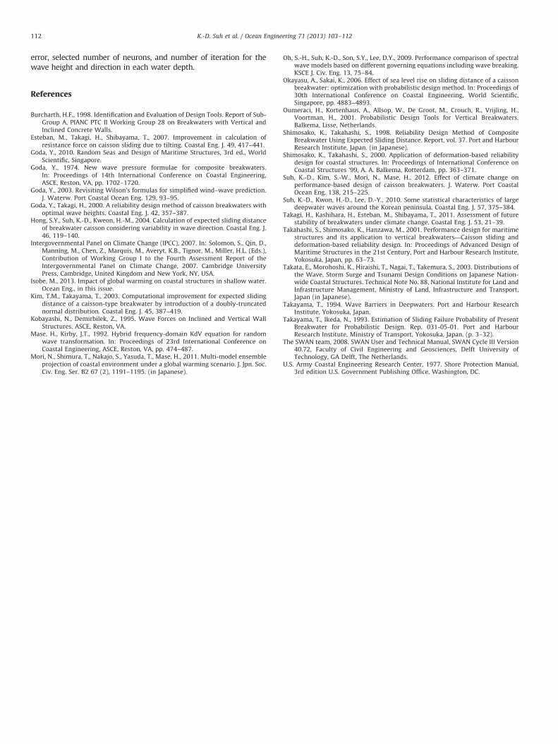
K.-D. Suh et al. / Ocean Engineering 71 (2013) 103–112112

error, selected number of neurons, and number of iteration for thewave height and direction in each water depth.

References

Burcharth, H.F., 1998. Identification and Evaluation of Design Tools. Report of Sub-Group A, PIANC PTC II Working Group 28 on Breakwaters with Vertical andInclined Concrete Walls.

Esteban, M., Takagi, H., Shibayama, T., 2007. Improvement in calculation ofresistance force on caisson sliding due to tilting. Coastal Eng. J. 49, 417–441.

Goda, Y., 2010. Random Seas and Design of Maritime Structures, 3rd ed., WorldScientific, Singapore.

Goda, Y., 1974. New wave pressure formulae for composite breakwaters.In: Proceedings of 14th International Conference on Coastal Engineering,ASCE, Reston, VA, pp. 1702–1720.

Goda, Y., 2003. Revisiting Wilson’s formulas for simplified wind–wave prediction.J. Waterw. Port Coastal Ocean Eng. 129, 93–95.

Goda, Y., Takagi, H., 2000. A reliability design method of caisson breakwaters withoptimal wave heights. Coastal Eng. J. 42, 357–387.

Hong, S.Y., Suh, K.-D., Kweon, H.-M., 2004. Calculation of expected sliding distanceof breakwater caisson considering variability in wave direction. Coastal Eng. J.46, 119–140.

Intergovernmental Panel on Climate Change (IPCC), 2007. In: Solomon, S., Qin, D.,Manning, M., Chen, Z., Marquis, M., Averyt, K.B., Tignor, M., Miller, H.L. (Eds.),Contribution of Working Group I to the Fourth Assessment Report of theIntergovernmental Panel on Climate Change, 2007. Cambridge UniversityPress, Cambridge, United Kingdom and New York, NY, USA.

Isobe, M., 2013. Impact of global warming on coastal structures in shallow water.Ocean Eng., in this issue.

Kim, T.M., Takayama, T., 2003. Computational improvement for expected slidingdistance of a caisson-type breakwater by introduction of a doubly-truncatednormal distribution. Coastal Eng. J. 45, 387–419.

Kobayashi, N., Demirbilek, Z., 1995. Wave Forces on Inclined and Vertical WallStructures. ASCE, Reston, VA.

Mase, H., Kirby, J.T., 1992. Hybrid frequency-domain KdV equation for randomwave transformation. In: Proceedings of 23rd International Conference onCoastal Engineering, ASCE, Reston, VA, pp. 474–487.

Mori, N., Shimura, T., Nakajo, S., Yasuda, T., Mase, H., 2011. Multi-model ensembleprojection of coastal environment under a global warming scenario. J. Jpn. Soc.Civ. Eng. Ser. B2 67 (2), 1191–1195. (in Japanese).

Oh, S.-H., Suh, K.-D., Son, S.Y., Lee, D.Y., 2009. Performance comparison of spectralwave models based on different governing equations including wave breaking.KSCE J. Civ. Eng. 13, 75–84.

Okayasu, A., Sakai, K., 2006. Effect of sea level rise on sliding distance of a caissonbreakwater: optimization with probabilistic design method. In: Proceedings of30th International Conference on Coastal Engineering, World Scientific,Singapore, pp. 4883–4893.

Oumeraci, H., Kortenhaus, A., Allsop, W., De Groot, M., Crouch, R., Vrijling, H.,Voortman, H., 2001. Probabilistic Design Tools for Vertical Breakwaters.Balkema, Lisse, Netherlands.

Shimosako, K., Takahashi, S., 1998. Reliability Design Method of CompositeBreakwater Using Expected Sliding Distance. Report, vol. 37. Port and HarbourResearch Institute, Japan. (in Japanese).

Shimosako, K., Takahashi, S., 2000. Application of deformation-based reliabilitydesign for coastal structures. In: Proceedings of International Conference onCoastal Structures ’99, A. A. Balkema, Rotterdam, pp. 363–371.

Suh, K.-D., Kim, S.-W., Mori, N., Mase, H., 2012. Effect of climate change onperformance-based design of caisson breakwaters. J. Waterw. Port CoastalOcean Eng. 138, 215–225.

Suh, K.-D., Kwon, H.-D., Lee, D.-Y., 2010. Some statistical characteristics of largedeepwater waves around the Korean peninsula. Coastal Eng. J. 57, 375–384.

Takagi, H., Kashihara, H., Esteban, M., Shibayama, T., 2011. Assessment of futurestability of breakwaters under climate change. Coastal Eng. J. 53, 21–39.

Takahashi, S., Shimosako, K., Hanzawa, M., 2001. Performance design for maritimestructures and its application to vertical breakwaters—Caisson sliding anddeformation-based reliability design. In: Proceedings of Advanced Design ofMaritime Structures in the 21st Century, Port and Harbour Research Institute,Yokosuka, Japan, pp. 63–73.

Takata, E., Morohoshi, K., Hiraishi, T., Nagai, T., Takemura, S., 2003. Distributions ofthe Wave, Storm Surge and Tsunami Design Conditions on Japanese Nation-wide Coastal Structures. Technical Note No. 88, National Institute for Land andInfrastructure Management, Ministry of Land, Infrastructure and Transport,Japan (in Japanese).

Takayama, T., 1994. Wave Barriers in Deepwaters. Port and Harbour ResearchInstitute, Yokosuka, Japan.

Takayama, T., Ikeda, N., 1993. Estimation of Sliding Failure Probability of PresentBreakwater for Probabilistic Design. Rep. 031-05-01. Port and HarbourResearch Institute, Ministry of Transport, Yokosuka, Japan. (p. 3–32).

The SWAN team, 2008. SWAN User and Technical Manual, SWAN Cycle III Version40.72, Faculty of Civil Engineering and Geosciences, Delft University ofTechnology, GA Delft, The Netherlands.

U.S. Army Coastal Engineering Research Center, 1977. Shore Protection Manual,3rd edition U.S. Government Publishing Office, Washington, DC.