Effect of Government Policies on

Urban and Rural Income Inequality

Ximing Wu,* Jeffrey M. Perloff,** and Amos Golan***

January 2006 * Department of Agricultural Economics, Texas A&M University;

xwu@ag.tamu.edu ** Department of Agricultural and Resource Economics, University of California,

Berkeley, member of the Giannini Foundation; perloff@are.berkeley.edu *** Department of Economics, American University; agolan@american.edu We are very grateful to the University of California Institute of Industrial Relations and the Giannini Foundation for financial support. Contact: Jeffrey M. Perloff Department of Agricultural & Resource Economics 207 Giannini Hall—MC 3310 University of California Berkeley, CA 94720-3310 510/642-9574 (office); 510/643-8911 (fax) perloff@are.berkeley.edu

Abstract

We use three conventional inequality indices—the Gini, the coefficient of

variation of income, and the relative mean deviation of income—and the Atkinson index

to examine the effect of income tax rates, the minimum wage, and all the major

government welfare and transfer programs on the evolution of income inequality for rural

and urban areas by state from 1981-1997. We find that these programs have

qualitatively similar but quantitatively different effects on urban and rural areas. Most

importantly, taxes are more effective in redistributing income in urban than in rural areas,

while welfare and other government transfer programs play a relatively larger role in

rural area.

Effect of Government Policies on Urban and Rural Income Inequality

Although income inequality has increased substantially in both urban and rural areas of

the United States over the past two decades, the levels of inequality in these areas have evolved

differently. We investigate whether these alternate paths are due to different responses to

changes in taxes, minimum wage laws, social insurance policies, and transfer programs. We find

that government policies have had qualitatively similar but quantitatively different effects on

rural and urban areas.1 Given these quantitative differences, some policies that effectively

reduce inequality in urban areas do not work well in rural areas.

Using Current Population Survey data for 1981 through 1997, we examine the effects of

eight major government policies on welfare using the Atkinson index as well three traditional

inequality measures: the Gini index, coefficient of variation of income, and the relative mean

deviation of income. In addition to examining the distributional impacts of government policy

variables, we determine how changes in macro conditions and demographic variables over time

and across the states affect inequality.

Our study differs from the literature in four ways. First, we examine the effects of many

policies and macro variables at once. Most previous studies considered the effect of only a

single policy, ignoring the influences of other government policies, market conditions, and

demographics (See references in Moffitt, 1992).

Second, we examine the effects of policies on the entire income distribution rather than

focusing on income effects of only low-paid workers as have most previous studies. Third, we

examine policy effects on both pre-tax and post-tax income inequality in urban and rural areas.

2

Fourth, and most importantly, we contrast urban and rural policy effects across the

nation.2 As Freeman (1996) observed, “Because the benefits and costs of the minimum

(wage)/other redistributive policies depend on the conditions of the labor market and the

operation of the social welfare system, the same assessment calculus can yield different results in

different settings.” According to Whitener et al. (2001), although the impact of the recent

welfare reform does not appear to differ greatly between rural and urban areas at the national

level, some studies on individual states report that the impact of welfare reform on employment

and earnings in the rural areas is smaller than in the urban areas.3 Instead of studying a single

state, we systematically examine the impacts of tax and welfare programs on family income

distribution across all states for each year from 1981 through 1997.

We find that the government policies have qualitatively similar but quantitatively

different impacts on the income inequality in rural and urban areas. Taxes have smaller

equalizing effects and government welfare and transfer programs have larger equalizing effects

in rural areas than in urban areas. These differential policy effects may be due to two main

differences in the composition of the population in these two areas. First, the proportion of the

population that needs to pay income tax and the proportion in the top tax bracket are higher in

urban areas. Second, a larger proportion of the rural population is eligible for welfare and

government transfer program (such as the low-income families and the elderly).

In the next section, we describe the data and the different government policies that we

analyze. We discuss the inequality measures in Section 3. Next we briefly describe the trends in

inequality in rural and urban areas. In Section 5, we use regressions to determine how policies

and macroeconomic conditions affect inequality in rural and urban areas. In Section 6, we

compare and contrast the rural and urban effects. We draw conclusions in the last section.

3

The Data

We construct a cross-section, time-series data set for the 50 U.S. states from 1981

through 1997. Our sample period starts in 1981, which is the year that the CPS started to impute

the value of taxes and governmental transfers of sampled families. Since the welfare reform

started in 1997, the traditional welfare program (Aid to Families with Dependent Children,

AFDC) was replaced by the Temporary Aid to Needy Families (TANF). We did not include

more recent years because we do not have a consistent and reliable set of the explanatory policy

variables that can capture the features of these two dramatically different programs. For

example, the chief change under TANF is that the recipient can be on the welfare for a lifetime

maximum of five years. Consequently, people responded strategically to the change by moving

in and out of the welfare due to the lifetime restraint. This substantial change in policy requires

carefully modeling of people’s dynamic welfare usage, which is beyond the scope of this study.

Therefore, our sample ends at 1997.

Our source of data for income and state demographic characteristics is the annual Current

Population Survey (CPS) March Supplements. The March CPS for a given year contains labor

market and income information for the previous year on between 50,000 and 62,000 households.

For each state, we calculate a range of inequality indices of annual family income for the

urban and rural areas.4 In some of the earlier years of our sample, the CPS did not cover both

areas for some of the smaller states. Consequently, we have 796 observations for the urban areas

and 718 observations for the rural areas.

The CPS total income measure, which is “the amount of money income received in the

preceding calendar year”, includes in-cash government transfers but not food stamps, other

4

government in-kind transfers, income tax payments or tax credit received. Therefore, the CPS

definition of income does not measure a family's entire disposable income.

Fortunately, beginning in the first year of our sample, 1981, the CPS imputed the value of

government transfers, tax liability and credit for each family. The Census Bureau combined data

from the American Housing Survey (AHS), the Income Survey Development Program (ISDP),

and the Internal Revenue Service (IRS) with CPS data to simulate the taxes paid, number of tax

filing units, adjusted gross income, and other tax characteristics for the March CPS.5 The Census

Bureau reported several definitions of income, ranging from the raw self-reported income, to

most ‘comprehensive’ income, which includes imputed government cash transfers, tax payments

and credits and value of noncash income, including food stamps, housing subsidies and medical

benefits. The food stamps are valued at its face value. According to Weinberg (2004) and

references therein, while calculation of equivalent market value of medical benefit is difficult,

the microsimulation model used by the Census Bureau to impute the value of tax payment and

credit is reasonably accurate. To minimize bias introduced by the imputation, we use a

‘conservative’ definition of after-transfer, after-tax income, which adjusts for the value of food

stamps, tax payment and credit of each family.

To control for family income variation due to family size, we divide the family income

by the total number of adult family members. To check the sensitivity of our inequality

estimates to the choice of equivalence scales, we consider three alternatives: (1) the total number

of family member; (2) the OECD equivalence scale (one for family head, 0.5 for each additional

adult, and 0.3 for each child), and (3) unity (no adjustment for family size). The results are not

sensitive to these normalizations.6

5

Government Policies

All the government policy variables vary over time and across states except the federal

income tax and disability insurance variables, which vary only over time. For detailed

information on Government policies during this period, see Meyer and Rosenbaum (2001) and

Wu et al. (2003).

We use two variables, the federal marginal income tax rate for the top bracket (Top Tax)

and for the tax bracket that has the largest share of taxpayers (Main Tax), to proxy the change of

federal income tax over the observed period. The state-specific data on the minimum wage and

maximum weekly unemployment insurance benefits are from the U.S. Bureau of Labor

Statistics’ Monthly Labor Review, which summarizes the previous year's state labor legislation.

Our Unemployment Insurance variable is the maximum weekly benefit in a state (almost all the

states set the maximum coverage period at 26 weeks during the relevant period).

Data on other public assistance programs are from the annual Background Material and

Data on Major Programs within the Jurisdiction of the Committee on Ways and Means (the

“Green Book”). Our minimum wage variable is the larger of the federal or the relevant state

minimum wage. If the minimum wage changed during the year, we use a time-weighted

average. Our Unemployment Insurance variable is the maximum weekly benefit in a state

(almost all the states set the maximum coverage period at 26 weeks during the relevant period).

Our disability (the inability to engage in “substantial gainful activity”) insurance measure is the

maximum annual benefit. The Supplement Security Income (SSI) variable is the maximum

monthly benefits for individuals living independently. To qualify for SSI payment, a person

must meet age, blindness or other disability standard and have an income below the federal

maximum monthly SSI benefit.

6

The AFDC variable is the maximum monthly benefits for a single-parent, three-person

family. The “AFDC need standard” variable is the maximum income a single-parent, three-

person family can have and still be eligible for assistance. The AFDC need eligibility standard is

used for the food stamps program as well. Our food stamps variable is the dollar value of the

maximum monthly benefit.

The Earned Income Tax Credit (EITC) program is an earning subsidy for the low income

working families. To receive an EITC, a family must have reported a positive earned income.

The EITC maximum benefit is determined by two factors: the EITC credit rate and the minimum

income requirement for maximum benefit. Our EITC Benefits variable measures the maximum

benefit, which is the product of these two factors. The EITC is phased out as a family's income

rises. For example, in 1997, the phase-out income range was ($11,930, $25,750) for a one-child

family. The credit is reduced by 15.98¢ for each extra dollar earned above $11,930 so that the

benefit drops to zero at $25,750. Here, our EITC phase-out rate variable measures the rate,

15.98 percent, at which the EITC benefits is reduced over the phase-out range. Beginning in

middle 1980’s, some states offered their own state EITC, usually in the form of a fixed percent

of the federal EITC credit. Our EITC benefit variable is adjusted by state supplements; hence

this measure varies across both states and time.

Macroeconomic and Demographic Variables

We include two macroeconomic variables to control for economic conditions. The U.S.

gross domestic product (GDP) and unemployment rates are from the Bureau of Labor Statistics'

website.7 In addition to state dummy variables, we include annual state-level demographic

characteristics obtained from the CPS: the percentage of the population with a high school

degree, the percentage of the population with at least a college degree, the percentage of female-

headed families, the percentage of the state's population in various age groups (younger than 18,

18-29, the residual group, and older than 59), and the average family size.

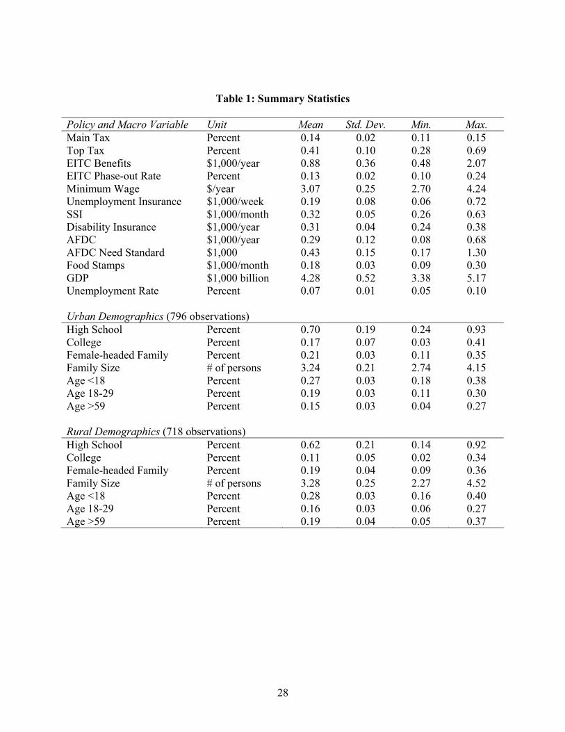
Table 1 contains the summary statistics for the sample. Compared to the urban

population, the rural population on average has a lower average education level, a smaller

fraction of female-headed families, a larger average family size, and a larger proportion of

elderly people.

<Place Table 1 about here>

Inequality Measures

We use the three traditional inequality measures as well as the Atkinson index. In

defining our welfare measures, we let y reflect income normalized by the sample mean, y*

7

dz

y

is the

highest observed income, f(y) is the density of income, F(y) is the income distribution, μ is the

empirical mean income, V is the standard deviation of y, and is the Lorenz

function. The three traditional welfare measures are:

( ) ( )0

yy zf zφ = ∫

• the coefficient of variation of income (COV): V/μ;

• the relative mean deviation of income (RMD): ; ( )*

0| 1|

yy f y d−∫

( ) ( ) ( )*

0

1 d .2

yyF y y f y yφ−⎡ ⎤⎣ ⎦∫ • the Gini index:

Atkinson (1970) popularized a welfare measure that we refer to as the “Atkinson index.”

This index has three strengths. First, the Atkinson index uses a single parameter to nest an entire

family of welfare measures that range from very egalitarian to completely nonegalitarian.

Second, it can be derived axiomatically from several desirable properties (Atkinson 1970;

Cowell and Kuga 1981). As Dalton and Atkinson (1970) argued compellingly, a measure of

inequality should be premised on a social welfare concept. They contended that a social welfare

function should be additively separable and symmetric function of individual incomes. Atkinson

imposed constant (relative) inequality aversion.

Third, the Atkinson index has a useful monetary interpretation. Corresponding to the

Atkinson index is an equally distributed equivalent level of income, yEDE, which is the level of

income per head that, if income were equally distributed equally across the population, would

give the same level of social welfare as the actual income distribution:

( ) ( ) ( ) ( )0 0

y y

EDEU y f y dy U y f y dy=∫ ∫ ,

where U(y) is an individual’s utility function. This measure is invariant to linear transformations

of the utility function. Atkinson’s welfare index is

1 EDEyIμ

= − , (1)

where μ is the actual average income. We can use this index to determine the percentage welfare

loss from inequality. For example, if I = 0.1, society could achieve the same level of social

welfare with only 90 percent of the total income if incomes were equally distributed. Our

measure of welfare loss from inequality, L, is the difference between the actual average income

and the equally distributed equivalent level,

EDEL yμ= − (2)

8

9

is a transformation of the Atkinson welfare index, Equation (1).

To impose constant relative inequality-aversion, Atkinson chose the representative utility

function

( )( )

1

11

ln 1

yA BU y

y

ε

εε

ε

−⎧+ ≠⎪= −⎨

⎪ =⎩

where ε ≥ 0 for concavity and ε represents the degree of inequality aversion. After some

algebraic manipulations involving Equations (1) and (2), Atkinson obtained his welfare index for

n people:

11 1

1

1

1

11 1

1 1

ni

i

n ni

i

yn

I

y

ε ε

ε

εμ

εμ

− −

=

=

⎧⎛ ⎞⎛ ⎞⎪ ⎜ ⎟− ≠⎜ ⎟⎪ ⎜ ⎟⎝ ⎠⎪ ⎝ ⎠= ⎨

⎪⎛ ⎞⎪ − =⎜ ⎟⎪ ⎝ ⎠⎩

∑

∏

. (3)

Atkinson’s index equals zero when income are equally distributed and converges to (but

never reaches) 1 as inequality increases. The index rises with ε. The larger is ε, the more weight

the index attaches to transfers at the low end of the distribution and the less weight to transfers at

the high end of the distribution. In the extreme case where ε → ∞, the welfare measure becomes

Rawlsian: Welfare depends on the income of the poorest member of society. If ε = 0, the utility

function is linear in income and the distribution of income does not affect the welfare index: Iε =

0 for any income vector. Thus, we view ε = 0 as a degenerate case and only look at ε that are

strictly positive. Following the suggestion in Atkinson (1970), we examine ε ≤ 2.

In our sample, the correlations between the inequality rankings from Atkinson indices

with ε in the range (0, 1] and the relative mean deviation, the coefficient of variation, and the

10

Gini index are close to one.8 Therefore, by choosing an appropriate value of ε, we could use Iε

to proxy the inequality ranking from the traditional inequality indices. Nonetheless, we report

these traditional welfare measures in our analyses because of their familiarity.

It is well known that sample estimates of inequality measures are subject to sample

variation and various difficulties, such as outliers, top-coding or imputed values, which might

lead to inefficient or even biased estimates. Cowell and Victoria-Feser (1996) note that the

estimates can be sensitive to these problems. We examine systematically the impact of outliers

and top-coding using the influence function approach proposed by Cowell and Victorira-Feser

(1996). We found that inequality measures consistent with risk aversion can be sensitive to

extremely low income values, while rather robust to top-coding (censoring at the high end of the

distribution). We applied the trimming method suggested by Cowell and Victoria-Feser (1996).

For details, see the original paper and the technical appendix of Wu et al. (2003). Nonetheless,

in the regression analysis below, we test the hypothesis of structural break in 1995 due to the

CPS redesign, which includes the change in top-coding procedure. The hypothesis is decisively

rejected.

Trends in Inequality

Income inequality as measured by each of the inequality measures rose substantially

during the sample period. However, the evolution of rural and urban inequality in individual

states varies substantially. For example, for states having data on both rural and urban areas

during the sample period, the average correlation between the rural and urban Gini indices is

only 0.45 using pre-tax income and 0.46 using post-tax income.

To save space, we discuss only the Gini index for both rural and urban areas, though all

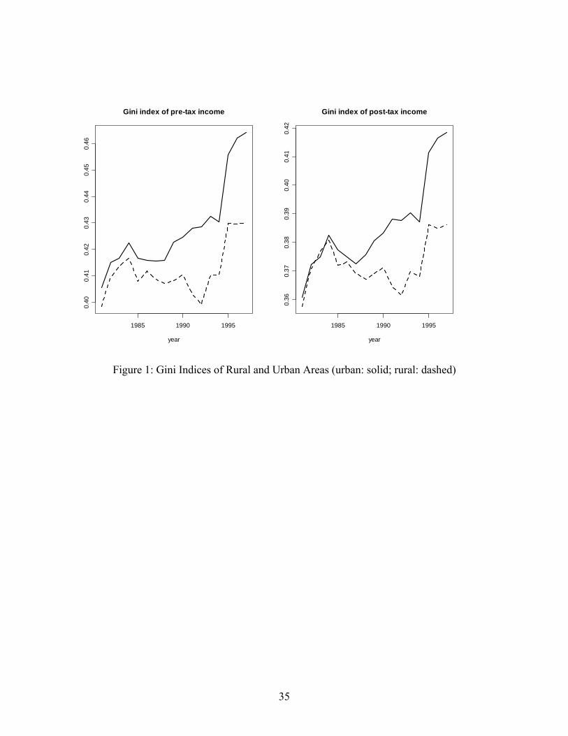
measures show similar patterns. The left panel of Figure 1 plots the Gini indices of pre-tax

11

income for the urban (solid) and rural (dashed) areas from 1981 through 1997. The urban Gini

inequality index is higher (less equal) in each year than the rural urban inequality and increases

by more over the sample period. Rural inequality increases from 0.398 to 0.430, while urban

inequality increases from 0.406 to 0.464. The Gini indices move together in the beginning of the

period and thereafter diverge. In both areas, inequality increases between 1981 and 1984, and

then declines slightly in the subsequent two or three years. Starting in 1988, urban inequality

began to rise quickly while rural inequality remained stable for another two more years and then

declined slightly between 1990 and 1992. Starting in 1994, both measures grew very rapidly for

a couple of years and then leveled off between 1996 and 1997.

The right panel of Figure 1 shows the Gini indices of post-tax income for both areas. The

post-tax Gini inequality measures are considerably smaller than the pre-tax measures: The Gini

is 0.042 lower for the urban area on average and 0.040 for the rural area. As with the pre-tax

indices, the post-tax Gini indices are nearly equal in the two areas from 1981 through 1984.

Thereafter, the rural and urban indices diverge: The urban income distribution became much

more unequal than the rural one.

<Place Figure 1 about here>

We can calculate the value of the welfare loss using the Atkinson index. For example,

the Atkinson index of pre-tax income with ε = 1 is 0.270 for urban areas and 0.261 for rural areas

in 1981. Using Equation (2), the corresponding welfare losses due to inequality are $1,912 and

$1,521 per person for this year. The same Atkinson index with ε = 1 increased to 0.340 for

urban areas and 0.297 for rural areas by the end of the sample in 1997. The welfare losses (in

1981 dollars) increased to $2,768 and $1,924 respectively, 34.0 percent of urban and 29.7

percent of rural average income.

Regression Analysis

We use regressions to examine the impacts of government policies on pre-tax and post-

tax rural and urban income inequality. We include in our model all the major government

programs that directly or indirectly transfer income to low-income families. The government tax

and transfer programs directly affect family income. The minimum wage, disability insurance,

and unemployment insurance have direct effects on people’s received income and indirect effects

on their transferred income because other government transfer programs are contingent on

earned income.

In Ashenfelter’s (1983) terminology, government policies have both “mechanical” and

“behavioral” effects. The mechanical effect measures the difference between the pre-tax income

and post-tax income due to tax payment to the government or transfers received from the

government. On the other hand, the policies also have behavioral implications: people may

respond to changes in these programs by changing their participation decision, hours of work, or

other labor market decisions (see, for example, Hausman (1981) for the labor supply effects of

tax and Moffitt (1992) for the incentive effects of welfare programs), which subsequently

influences their earnings. Therefore, the government policies can impact the income distribution

through two channels and the effects on pre-tax income and post-tax income may differ.

We estimate cross-sectional, time-series regression models with first-order autoregressive

error terms:

it it i itw a u e= + + +X β ,

where

1it it ite e zρ −= + ,

12

13

wit is the inequality or welfare index for either the urban or rural area, Xit is a vector of the

explanatory variables, the subscript i indexes the states, t indexes the year, |ρ| < 1, and zit is

independent and identically distributed (IID) with zero mean and variance σz. We estimate a

random-effect model in which the state effects are captured by ui, realization of an IID process

with zero mean and variance σu.9 Due to the unbalanced panel structure of our data, we use the

methods derived in Baltagi and Wu (1999).

The explanatory variables included in X are the percentages of the population finishing

high school and finishing college; the percentage of female-headed families; average family size;

the percentage of the population under age 18, between 18 and 29, and than 59; the marginal

income tax rates for the lowest and the highest tax bracket; the EITC benefit and phase-out rate;

the minimum wage; the UI benefit; the SSI benefit; the disability insurance benefit; the AFDC

benefit and need standard; the food stamps benefit; the GDP; and the unemployment rate.

We estimated the model for each of our measures of inequality: the three traditional

inequality measures and the Atkinson index for a wide range of values of the “inequality

aversion” parameter ε. We report the Atkinson measure for only ε equal 0.5, 1, and 2, which are

social welfare functions with relatively low-, medium- and high-degrees of inequality aversion.

We do not report the results for the deviation in logarithms and Atkinson indices for other values

of ε because they are similar to those reported.

Although the policy effects are qualitatively similar in the rural and urban areas, we reject

the hypothesis that the two sets of regression coefficients are equal using Chow tests. For each

inequality measure, the restriction is rejected decisively (the p-values essentially equal zero).

Thus, the policies and macro variables seem to quantitatively different effects across the two

areas. However, a closer examination reveals their difference. We test separately if the

14

coefficients for the macro variables and policy variables are the same across the two areas. The

Chow statistic for the test on macro variable has a p-value of 0.28, hence we fail to reject the

hypothesis that the coefficients of macro variables are identical. At the same time, the Chow

statistic for the test on policy variables has a p-value of 0.0016 when we assume identical

coefficients for the macro variables. Not surprisingly, the p-value changes only slightly (to

0.0012) when we conduct the same test on the policy variables, allowing for different

coefficients for macro variables.

Because the pattern of urban and rural inequality started to diverge in 1990, we test the

hypothesis that the policy effects systematically changed in 1990. We cannot reject the null

hypothesis of no structural break using a likelihood ratio test in which we compare the pooled

regression to separate regressions for the period up to 1989 and from 1990 on. Similarly, we

cannot reject the hypothesis of no structural break in 1995.

The Urban Areas

Tables 2 and 3 report the regression results for pre-tax and post-tax income inequality for

the urban area. The coefficients are qualitatively similar across all the inequality measures for

both pre-tax and post-tax income. The estimated auto-correlation coefficients are less than 0.3,

indicating modest auto-correlation of income inequality. The share of the variation that is due to

the random state effects, ui, is around one third to one half, depending on the dependent variable.

The R2 ranges from 0.27 through 0.43. On the average, about 45 percent of the variation

explained by the model is due to the policy variables for both pre-tax and post-tax inequality.

For example, the R2 of the pre-tax Gini regression is 0.39, of which 44 percent of the explained

variation is attributed to the policy variables. The R2 for the post-tax Gini is 0.38, and 46 percent

of the variation explained by the model is due to the policy variables.

15

<Place Table 2 and Table 3 about here>

Most of the government policy variables have the expected signs as suggested by the

literature (see, for example, Bishop et al. 1994 and references therein). As expected, an increase

in the marginal income tax rate for the main tax bracket has an equalizing effect on both pre-tax

and post-tax income that is statistically significantly different than zero at the 0.05 level in all the

post-tax regressions and most of the pre-tax ones. In contrast, the marginal income tax rate for

the top tax bracket only has statistically significant equalizing effects for the post-tax income, as

indicated by the Gini index and the Atkinson index with ε = 0.5 and 1. Compared with the

Atkinson index with larger ε, these indices place relative high weights on the high end of the

distribution and are therefore more sensitive to changes at the high end of the distribution.

As we expected, the EITC benefit—which supplements the incomes of poor working

families—does not statistically significantly affect pre-tax inequality but does statistically

significantly affect the post-tax income inequality for all the reported inequality measures except

for the coefficient of variation of income and I2. This finding is consistent with the literature that

the EITC plays an important role in increasing the income of the working poor and reduces

income inequality (Neumark and Washer 2001 and Wu et al. 2003).

The EITC phase-out rate is the marginal rate by which earnings above a specified

threshold reduce the EITC benefit. An increase in the EITC phase-out rate reduces the labor

supply of those people with earning above that threshold who are eligible for the EITC.

Consequently, increases in the phase-out rate lower the earnings of some people in this group.

Eissa and Hoynes (1998) and Wu (2003) found that the EITC phase-out rate has substantial

disincentive effects on the labor supply of the affected population, and therefore may reduce

their pre-tax and post-tax income. Because EITC recipients tend to be low-income families

16

whose primary source of income is earnings, the resulting drop in their income may have

substantial reduce equality. In most of our regressions, the EITC phase-out variable statistically

significantly raises inequality for both pre-tax and post-tax income distributions.

Although an increase in minimum wage raises the wage floor, individuals who were

previously earning a wage between the original and new minimum wage rate may lose their jobs

or be forced to reduce their hours because of the unemployment effects of the minimum wage.

Moreover, the minimum wage is not a means-tested program. Unlike the welfare and other

government transfer programs, all workers are entitled to earn at least the minimum wage.

Burkhauser et al. (1996) observe that minimum wage workers are evenly distributed across all

family income groups, in large part because many of them are teenage workers from relatively

well-off families. However, the disemployment effect is disproportionately concentrated among

low-income families. Therefore, raising the minimum wage may raise inequality (Neumark et

al., 1998 and Wu et al., 2003). In our regression, an increase in our minimum wage variable,

which is the higher of the federal and state minimum wages in each state in each year, raises both

pre-tax and post-tax income inequality (the effect is statistically significant for all inequality

measures except I2).

The disability insurance and AFDC program reduce both the pre-tax and post-tax income

inequality (statistically significantly in most equations). Unlike tax payments and the EITC

benefit, the value of AFDC is included in the CPS’s pre-tax income measure. Therefore, we

expect to see similar effects of the AFDC benefit variable on both pre-tax and post-tax income.

The remaining policy variables—unemployment insurance, supplemental social insurance, the

need standard for the AFDC program, and food stamps—do not have statistically significant

effects on pre-tax or post-tax income inequality.

17

Some of the demographic characteristics have statistically significant effects on

inequality. Consistent with the literature, we find that a rise in the share of female-headed

families plays an important role in increasing income inequality. For both the pre-tax and post-

tax income distribution, the percentage of female-headed family shows the most statistically

significant effects among all the explanatory variables. States with a high proportion of large

families have less equal income distributions. States with a large share of families with heads

who are younger than 18 tend to have less equal incomes. However, age of the family head does

not otherwise have statistically significantly effects on inequality.

The larger the percentage of the population with at least a high school education, the less

income inequality (though this effect is statistically significant in only some of the regressions).

A larger percentage of college graduates makes the income distribution less equal (statistically

significantly in most equations). These finding are consistent with the hypothesis of skill-based

technological change (SBTC) in the literature: The wage/income premium for college graduates

compared to low-skilled workers has been increasing during the last two decades, partially due to

the shift in labor demand away from unskilled workers.10 (See Card and DiNardo (2002) for a

critical review of this literature.) A rise in GDP leads to greater income inequality. Surprisingly,

shifts in the unemployment rate have little effect.

The Rural Areas

Table 4 and 5 report the corresponding results for rural areas. The regression results on

the rural area are similar to the urban ones across the various inequality measures for both the

pre-tax and post-tax income distributions. The autocorrelation coefficients, ρ, lie between 0.12

to 0.23. The share of the residual that is attributed to the random state effects is between one-

fifth to slightly over one-third. The R2 ranges from 0.17 through 0.4. On the average, about 40

18

percent of the variation explained by the model is due to the policy variables for both pre-tax and

post-tax inequality. For example, the R2 of the pre-tax Gini regression is 0.38, of which 39

percent of the explained variation is due to the policy variables. The R2 for post-tax Gini is 0.36,

and 42 percent of the variation explained by the model is due to the policy variables.

<Place Table 4 and Table 5 about here>

The statistically significant qualitative government policy effects are similar to those in

the urban areas. The marginal income tax rate for the main tax bracket has a statistically

significant equalizing effect on both the pre-tax and post-tax income distributions, while the tax

rate for the top income bracket does not have a statistically significant effect.

For most of the inequality measures for both pre-tax and post-tax income, a larger EITC

benefit decreases the income inequality while its phase-out rate increases inequality. The

minimum wage variable has little effect. Of the remaining government policy variables, only the

AFDC benefit has a statistically significant (equalizing) effect on the income distribution.

The demographic and macro economic indicator variables generally have the same

qualitative effects as in the urban areas. The income inequality decreases as the share of the

population that finished high school increases or as the share of college graduates decreases. The

percentage of female-head families has statistically significantly increases inequality. The

average family size has little effect. Again, inequality is greater, the larger the share of families

headed by people younger than 18. However, age otherwise has little effect. Finally, income

inequality increases with the GDP, but does not appear to respond to changes in unemployment

rate.

19

Urban and Rural Comparison

To see how the variables with statistically significant effects—marginal income tax rates,

EITC variables, the minimum wage, and GDP—affect various measures of inequality, we first

calculate the elasticities of inequality for each policy variable evaluated at the sample averages.

Next, we calculate the dollar value of the welfare effects.

Elasticities

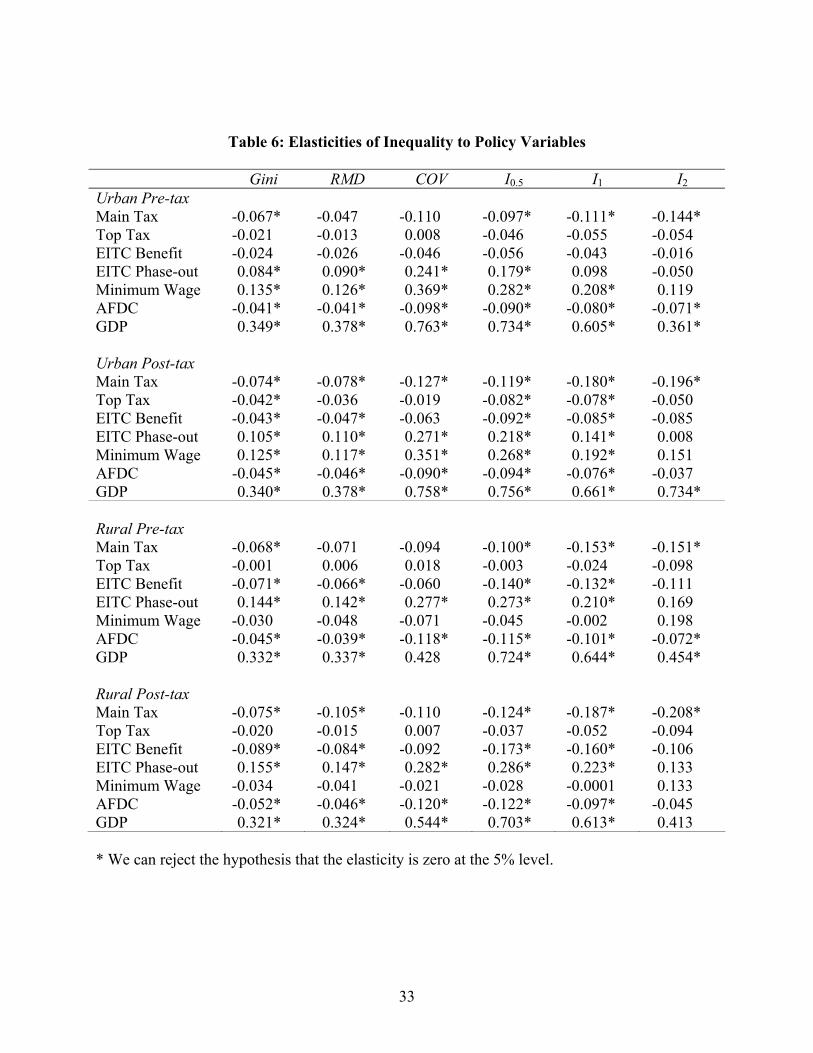
The top panel of Table 6 reports the estimated urban elasticities, and the bottom panel

lists the rural elasticities. For example, the sixth cell in the first column of numbers (post-tax

panel) of Table 6 shows that that the post-tax, urban Gini elasticity with respect to minimum

wage is 0.14. That is, when the minimum wage rises by 1 percent, the urban Gini increases by

0.14 percent. In both tables, the post-tax elasticity is almost always larger in absolute value than

is the pre-tax elasticity (and more likely to be statistically significantly different from zero).

<Place Table 6 about here>

Increasing the marginal rate on the main tax bracket or the rate on the top bracket tends to

reduce inequality in both areas. The Main Tax has statistically significant effects (except for the

coefficient of variation of income measure) on both pre- and post-tax inequality in urban and

rural areas. The effects in rural areas are slightly larger in absolute value. In urban areas, the

Top Tax does not have statistically significant effects on the pre-tax inequality, but does have

statistically significant equalizing effects on the post-tax urban Gini, the relative mean deviation

of income, and the I0.5 inequality measures. The pre-tax and post-tax Top Tax effects are not

statistically significant in rural areas. One possible explanation for why Top Tax has more of an

effect in equalizing income in urban than in rural areas is that relatively few rural dwellers are in

the top tax bracket.11

20

Transfer programs tend to have bigger effects in rural areas where relatively more

families are eligible for government transfers because of low income or age. For the same

reason as with taxes, the post-tax effects of government transfer programs are generally larger (in

absolute value) than pre-tax effects.

The two EITC elasticities are considerably larger in rural than in urban areas, especially

the ETIC benefit. The EITC benefit has a statistically significant effect on both pre- and post-tax

inequality in rural areas (except for the coefficient of variation of income and I2). In urban areas,

the EITC benefit does not have a statistically significant effect on pre-tax inequality, but does

have a statistically significant equalizing effect on the post-tax Gini, relative mean deviation of

income, and the I0.5 inequality measures. The EITC phase-out rate increases both pre-tax and

post-tax inequality, with a larger effect in the rural areas.

One major difference between the urban and rural areas is that the minimum wage has

large, statistically significant effects in urban areas, but does not have a statistically significant

effect in the rural areas. A plausible explanation is that the minimum wage law is less likely to

be enforced in rural areas. Moretti and Perloff (2000) find that many agriculture workers are

paid less than the minimum wage (unlike most other workers). Because the minimum wage

directly influences the earned income and does not involve any transfer from the government, the

urban pre-tax and post-tax minimum wage effects are close. The post-tax effects are slightly

smaller, possibly because losses in income due to an increase in the minimum wage induced

unemployment are offset by government transfers.

Growth of the economy (GDP) causes inequality to increase substantially. The effects

are roughly equal in rural and urban areas for all the welfare measures. A 10 percent increase in

GDP causes the pre- and post-tax Gini to rise by roughly 3 percent and I1 to increase by 6 to 7

percent in both areas.

Magnitude of Policy Effects

We can also compare the magnitude of policy effects using the dollar-value interpretation of

the Atkinson measures. (There is no simple way to compare the magnitude of these effects using

traditional measures.) We illustrate the magnitude of the welfare effects of some key

government policy and other variables in our analysis using the change in the welfare loss, L = μ

- y

21

EDE, Equation (2), which is the actual average income, μ, less the equally distributed

equivalent level of income, yEDE.

Our measure of a policy’s welfare effect is a dollar value interpretation of the change in

the aggregate social welfare and depends on the choice of ε: the degree of inequality aversion.

This estimate is based on the distribution of family disposable income, which reflects the impact

of policy changes on both the benefit calculation (the direct/mechanical effect) and the induced

responses in labor market behavior (the indirect/behavioral effect). Therefore, the reported

welfare benefit/cost should not be confused with the traditional benefit/cost analysis, which does

not take into account either the social welfare function or the potential behavior effects of

changes in policies.

If we raise the 1997 level of the Main Tax rate by 10 percent, from 15 percent to 16.5

percent, the Atkinson index changes to , where I εMain Taxˆ 0.165I I εε β′ = + × is the estimated

actual Atkinson index for 1997 family income and is the estimated coefficient for the

Main Tax. Assuming that the change in taxes does not have general equilibrium effects, the

change in welfare loss due to lack of equality is [using Equation

Main Taxβ

(1)]

( ) ( ) ( )97 97 97 97ˆ ˆ ˆˆ ˆ( ) ( ) 1 1EDE EDEL y y I I Iε ε εμ μ μ μ⎡ ⎤′ ′Δ = − − − = − − − = −⎣ ⎦

ˆ ,Iε′

where the urban μ97, the arithmetic mean in 1997 dollars of family income per person, is

$14,405, pre-tax, and $11,458, post-tax, while the corresponding rural averages are $12,878 and

$10,545.

Table 7 shows the average welfare losses (or gains) for ε = 0.5, 1, and 2 when we

increase each policy variable by 10 percent. Across the ε’s, the largest equalizing welfare

effects is for the marginal tax rate for the main tax bracket. For example, when ε = 0.5, a 10

percent increase in this marginal tax rate increases the average pretax welfare by $22 in urban

areas and $17 in rural areas, and the corresponding post-tax welfare effects are $19 and $16. To

calculate the overall effects, we multiply by the corresponding urban or rural population in 1997.

We find that this tax changes increases pretax welfare by $4.69 and $0.92 billion dollars in urban

and rural areas and post-tax welfare by $4.05 and $0.87 billion dollars. Strikingly, this welfare

effect is larger than the direct effect from a 10 percent increase in AFDC payment.

<Place Table 7 about here>

A 10 percent increase in the minimum wage has the greatest disequalizing effect in urban

areas. For ε = 0.5, a 10 percent increase in the minimum wage leads to a per person urban

welfare loss of $58 pretax and $40 post-tax but has no effect on rural welfare, or $12.3 and $8.5

billion respectively at the aggregated level.

Summary and Conclusions

This study is the first to investigate and compare the effects of all major income

redistribution policies on inequality in the urban and rural areas using data from across the

United States. During the past two decades, income inequality has increased considerably in

22

23

both rural and urban areas in response to changes in these policies, shifts in demographics, and

macro conditions.

We systematically examine the effects of income tax rates, the minimum wage, and all

the major government welfare and transfer programs on family income inequality. We find that

it is feasible to study welfare effects of policies because the qualitative results are generally the

same across most major inequality measures. Slightly less than half of the explained variation in

our regression analyses is due to policy variables (rather than to macro conditions and

demographic characteristics).

To our knowledge, this study is the first to clearly distinguish between pre-tax and post-

tax results for a variety of policies. To the degree that many earlier studies have ignored taxes,

they may consequently be biased. Pre-tax policy effects on the inequality level differ from post-

tax effects. The impacts of the policies involving income transfers between the government and

the individuals, such as tax rates and the Earned Income Tax Credit, are larger for the post-tax

income inequality. However, we also observe substantial changes in pre-tax inequality for other

policies that have substantial incentive effects on individual labor market behavior. For policies

that do not involve direct transfers, such as the minimum wage, we observe comparable effects

on pre-tax and post-tax income inequality.

Studies that do not distinguish between the effects of policies in rural and urban areas

may not be adequately informative. We find that, although the effects of welfare reform and

other policies on income inequality are qualitatively similar across rural and urban areas, they

differ quantitatively. This difference in impact plays a large role in explaining why the average

correlation between the rural and urban Gini indices over a couple of decades is less than half.

24

Our results show that policy evaluation should be conducted at the appropriate level of

aggregation because over-aggregation gives misleading results. In particular, we find that if

researchers ignore difference between rural and urban areas and aggregate across these areas,

they may falsely conclude those policies that are effective in urban areas also work in rural areas

and vice versa or those policies that have significant effects at a regional level do not have an

effect at a national level.

Some policies, such as the marginal tax rate on the main tax bracket and the Earned

Income Tax Credit have as large or larger effects on equalizing income in rural areas as in urban

areas. However, the marginal tax rate on the highest income bracket has an important effect on

inequality only in urban areas. This difference may be due to the relatively small fraction

families with high incomes in rural areas. The minimum wage has large, statistically significant

effects in urban areas, but does not have a statistically significant effect in rural areas. In

contrast, the EITC has a greater impact in rural than in urban areas.

Currently, Republicans often call for tax cuts whereas Democrats often emphasize using

minimum wage laws and direct welfare programs. These leaders may not realize the differential

impacts that their programs have for urban versus rural areas. Provided that a leader wants a

more equitable income distribution in his or her district, a representative with an urban

constituency should advocate adjusting taxes or the minimum wage, whereas a rural

representative should emphasize direct assistance such as the EITC.

25

References

Ashenfelter, Orley, “Determining Participation in Income-Tested Social Programs,” Journal of

American Statistical Association 78, 517-25, September 1983.

Atkinson, Anthony B, “Income Inequality in OECD Countries: Data and Explanations,”

Working Paper, CESifo, 2003.

Atkinson, Anthony B, “Is Rising Inequality Inevitable?” Annual Lecture, WIDER, 1999.

Atkinson, Anthony B, “On the Measurement of Inequality,” Journal of Economic Theory 2, 244-

63, September 1970.

Baltagi, Badi H. and Ping X. Wu, “Unequally Spaced Panel Data Regressions with AR(1)

Disturbances,” Econometric Theory, 15, 814-823, December 1999.

Bishop, John A., John P. Formby, and Ryoichi Sakano, “Evaluating Changes in Distribution of

Income in the United States,” Journal of Income Distribution, 4, 79-105, 1994.

Burkhauser, Richard V., Kenneth A. Couch, and David C. Wittenburg, “‘Who Gets What’ from

Minimum Wage Hikes: A Re-Estimation of Card and Krueger's Distributional Analysis

in Myth and Measurement: The New Economics of the Minimum Wage,” Industrial and

Labor Relations Reviews, 49, 547-64, April 1996.

Card, David and John E. DiNardo, “Skill-Biased Technology Change and Rising Wage

Inequality: Some Problems and Puzzles,” Journal of Labor Economics, 20, 733-783,

October 2002.

Cowell, Frank A., and Maria-Pia Victoria-Feser, “Robustness Properties of Inequality

Measures,” Econometrica, 64, 77-101, January 1996.

Dahl, Gordon B., “Mobility and Return to Education: Testing a Roy Model with Multiple

Markets.” Econometrica, 70, 2367-2420, November 2002.

26

Dalton, Hugh, “The Measurement of the Inequality of Incomes,” Economic Journal, 30, 348-

361, 1920.

Eissa, Nada, and Hillary W. Hoynes, “The Earned Income Tax Credit and the Labor Supply of

Married Couples,” working paper, NBER, 1998.

Freeman, Richard B., “The Minimum Wage as a Redistributive Tool?” Economic Journal, 104,

639-649, May 1996.

Gottschalk, P. and Danziger, S. “Family Income Mobility—How Much is There, and Has it

Changed?” in Alan J. Auerbach and Richard Belous, eds., The Inequality Paradox:

Growth of Income Disparity, 92-111, National Policy Association, Washington, D.C.,

1998.

Hausman, Jerry A., “Labor Supply,” in H. J. Aaron and J. A. Pechman, eds., How Taxes Affect

Economic Behavior, 27-72, Brookings Institution, Washington, D.C., 1981.

Kilkenny, Maureen and Sonya Kostova Huffman, “Rural/Urban Welfare Program and Labor

Force Participation,” American Journal of Agricultural Economics, 85, 914-927,

November 2003.

Meyer, Bruce D. and Dan T. Rosenbaum. “Welfare, the Earned Income Tax Credit, and the

Labor Supply of Single Mothers,” Quarterly Journal of Economics, 116, 1063-1114,

August 2001.

Moretti, Enrico and Jeffrey M. Perloff, “Minimum Wage Laws Lower Some Agricultural

Wages,” Working Paper, University of California, Berkeley, 2000.

Moffitt, Robert, “Incentive Effects of the U.S. Welfare System: A Review.” Journal of

Economic Literature, 30, 1-61, March 1992.

27

Neumark, David, Mark Schweitzer, and William Wascher, “The Effects of Minimum Wages on

the Distribution of Family Incomes: A Non-Parametric Analysis,” working paper, NBER,

1998.

Neumark, David and William Wascher, “Using the EITC to Help Poor Families: New Evidence

and a Comparison with the Minimum Wage,” National Tax Journal, 54, 281-317, June

2001.

RUPRI Rural Welfare Reform Research Panel, “Welfare Reform in Rural America: A Review of

Current Research,” Rural Policy Research Institute, 2001.

Smeeding, T. M. “U.S. Income Inequality in a Cross-national Perspective: Why Are We So

Different?” in Alan J. Auerbach and Richard Belous, eds., The Inequality Paradox:

Growth of Income Disparity, 194-217, National Policy Association, Washington, D.C.,

1998.

Whitener, Leslie A., Bruce A. Weber, and Greg J. Duncan, “Reforming Welfare: Implications

for Rural America,” Rural America, 16, 2-10, Fall 2001.

Weinberg, Daniel H. “Income Data Quality Issues in the Annual Social and Economic

Supplement to the Current Population Survey,” paper prepared for the American

Enterprise Institute-University of Maryland Seminar on Poverty Measurement October

12, 2004.

Wu, Ximing, “Three Essays on Government Policy, Labor Supply and Income Distribution.”

Ph.D. Thesis, University of California at Berkeley, 2003.

Wu, Ximing, Jeffrey M. Perloff, and Amos Golan, “Effects of Government Policies on Income

Distribution and Welfare,” working paper, University of California at Berkeley, 2005.

28

Table 1: Summary Statistics

Policy and Macro Variable Unit Mean Std. Dev. Min. Max. Main Tax Percent 0.14 0.02 0.11 0.15 Top Tax Percent 0.41 0.10 0.28 0.69 EITC Benefits $1,000/year 0.88 0.36 0.48 2.07 EITC Phase-out Rate Percent 0.13 0.02 0.10 0.24 Minimum Wage $/year 3.07 0.25 2.70 4.24 Unemployment Insurance $1,000/week 0.19 0.08 0.06 0.72 SSI $1,000/month 0.32 0.05 0.26 0.63 Disability Insurance $1,000/year 0.31 0.04 0.24 0.38 AFDC $1,000/year 0.29 0.12 0.08 0.68 AFDC Need Standard $1,000 0.43 0.15 0.17 1.30 Food Stamps $1,000/month 0.18 0.03 0.09 0.30 GDP $1,000 billion 4.28 0.52 3.38 5.17 Unemployment Rate Percent 0.07 0.01 0.05 0.10 Urban Demographics (796 observations) High School Percent 0.70 0.19 0.24 0.93 College Percent 0.17 0.07 0.03 0.41 Female-headed Family Percent 0.21 0.03 0.11 0.35 Family Size # of persons 3.24 0.21 2.74 4.15 Age <18 Percent 0.27 0.03 0.18 0.38 Age 18-29 Percent 0.19 0.03 0.11 0.30 Age >59 Percent 0.15 0.03 0.04 0.27 Rural Demographics (718 observations) High School Percent 0.62 0.21 0.14 0.92 College Percent 0.11 0.05 0.02 0.34 Female-headed Family Percent 0.19 0.04 0.09 0.36 Family Size # of persons 3.28 0.25 2.27 4.52 Age <18 Percent 0.28 0.03 0.16 0.40 Age 18-29 Percent 0.16 0.03 0.06 0.27 Age >59 Percent 0.19 0.04 0.05 0.37

29

Table 2: Regression Results Of Pre-Tax Inequality For The Urban Areas

Dependent Gini RMD COV I0.5 I1 I2

Variable Coef. t-stat Coef. t-stat Coef. t-stat Coef. t-stat Coef. t-stat Coef. t-statHigh School -0.032 -2.45 -0.055 -2.80-0.064 -1.01 -0.021-2.30 -0.036 -2.22 -0.051-1.26College 0.087 2.50 0.127 2.39 0.043 0.26 0.055 2.23 0.107 2.48 0.192 1.91Female Head 0.264 8.11 0.370 7.52 0.747 4.92 0.205 8.95 0.432 10.77 0.906 9.48Family Size 0.026 2.94 0.038 2.90 0.078 1.99 0.020 3.24 0.041 3.85 0.099 4.04Age <18 0.178 2.59 0.251 2.40 0.430 1.33 0.122 2.50 0.212 2.48 0.117 0.58Age 18-29 0.012 0.23 0.027 0.36-0.191 -0.80 0.000 0.01 0.006 0.10 -0.073-0.48Age >59 0.072 1.35 0.097 1.20 0.050 0.20 0.045 1.19 0.086 1.31 0.055 0.35Main Tax -0.002 -2.15 -0.002 -1.78-0.007 -1.85 -0.001-2.25 -0.002 -2.41 -0.006-2.33Top Tax -0.021 -1.12 -0.019 -0.67 0.018 0.19 -0.016-1.23 -0.038 -1.63 -0.075-1.28EITC Benefit -0.011 -1.14 -0.017 -1.20-0.046 -0.99 -0.009-1.33 -0.014 -1.21 -0.010-0.33EITC Phase-out 0.265 2.22 0.404 2.23 1.618 2.79 0.195 2.31 0.210 1.42 -0.219-0.59Minimum Wage 0.018 3.07 0.024 2.75 0.105 3.73 0.013 3.22 0.019 2.60 0.022 1.26Unemployment Ins. -0.001 -0.06 -0.001 -0.06 0.031 0.61 0.001 0.18 0.005 0.38 0.056 1.68SSI -0.019 -0.47 -0.022 -0.37 0.081 0.50 -0.012-0.45 -0.019 -0.39 0.074 0.75Disability Ins. -0.059 -2.63 -0.071 -2.12-0.394 -3.47 -0.044-2.77 -0.067 -2.42 -0.117-1.58AFDC -0.057 -2.56 -0.082 -2.41-0.294 -3.4 -0.044-2.88 -0.077 -2.84 -0.140-2.63AFDC Need Std. 0.009 1.05 0.012 0.97 0.006 0.16 0.005 0.87 0.012 1.17 0.020 0.88Food Stamps 0.026 0.42 0.031 0.33-0.086 -0.33 0.021 0.47 0.088 1.15 0.403 2.49GDP 0.033 4.34 0.051 4.50 0.154 4.00 0.024 4.46 0.039 4.13 0.059 2.36Unemployment Rate 0.002 0.90 0.004 1.41-0.004 -0.41 0.001 0.83 0.003 1.40 0.008 1.45Constant 0.045 0.77 0.029 0.32-0.445 -1.59 -0.123-2.95 -0.199 -2.74 -0.240-1.34ρ 0.289 0.300 0.206 0.281 0.295 0.117 σu 0.016 0.025 0.045 0.011 0.019 0.028 σz 0.018 0.027 0.088 0.013 0.022 0.057 R2 0.395 0.373 0.406 0.429 0.431 0.271

30

Table 3: Regression Results Of Post-Tax Inequality For The Urban Areas

Dependent Gini RMD COV I0.5 I1 I2

Variable Coef. t-stat Coef. t-stat Coef. t-stat Coef. t-stat Coef. t-stat Coef. t-statHigh School -0.022 -1.85 -0.039 -2.21-0.036 -0.66 -0.013-1.72 -0.022 -1.65 -0.029-0.76College 0.072 2.31 0.103 2.20 0.037 0.27 0.039 1.97 0.071 2.00 0.063 0.67Female Head 0.232 7.99 0.328 7.52 0.568 4.39 0.159 8.59 0.343 10.27 0.846 9.47Family Size 0.021 2.68 0.030 2.54 0.065 1.94 0.015 3.08 0.033 3.65 0.088 3.91Age <18 0.173 2.81 0.254 2.74 0.455 1.65 0.092 2.35 0.135 1.90 -0.127-0.67Age 18-29 0.012 0.28 0.038 0.56-0.128 -0.63 -0.003-0.10 -0.008 -0.16 -0.153-1.09Age >59 0.049 1.02 0.077 1.08 0.035 0.17 0.023 0.75 0.037 0.68 -0.089-0.61Main Tax -0.002 -2.99 -0.003 -2.61-0.007 -2.05 -0.001-3.11 -0.003 -3.42 -0.007-3.11Top Tax -0.038 -2.25 -0.046 -1.82-0.036 -0.46 -0.023-2.11 -0.044 -2.27 -0.060-1.07EITC Benefit -0.018 -2.17 -0.028 -2.27-0.054 -1.35 -0.012-2.24 -0.022 -2.31 -0.047-1.57EITC Phase-out 0.297 2.79 0.445 2.78 1.572 3.18 0.192 2.82 0.247 2.01 0.031 0.09Minimum Wage 0.015 2.84 0.020 2.58 0.086 3.59 0.010 3.01 0.014 2.38 0.024 1.43Unemployment Ins. 0.001 0.12 0.001 0.05 0.026 0.61 0.002 0.39 0.007 0.64 0.042 1.29SSI -0.018 -0.51 -0.022 -0.41 0.026 0.19 -0.011-0.49 -0.013 -0.31 0.092 1.03Disability Ins. -0.043 -2.13 -0.051 -1.72-0.278 -2.87 -0.029-2.25 -0.044 -1.89 -0.060-0.83AFDC -0.057 -2.85 -0.083 -2.74-0.233 -3.14 -0.037-2.95 -0.060 -2.69 -0.063-1.30AFDC Need Std. 0.008 1.08 0.010 0.93 0.021 0.66 0.005 0.98 0.009 1.07 0.016 0.78Food Stamps 0.023 0.41 0.025 0.30-0.009 -0.04 0.012 0.34 0.054 0.85 0.364 2.48GDP 0.029 4.36 0.046 4.55 0.132 4.03 0.020 4.57 0.035 4.43 0.083 3.40Unemployment Rate 0.001 0.51 0.003 1.09-0.004 -0.48 0.000 0.47 0.002 1.09 0.009 1.65Constant 0.067 1.28 0.063 0.80-0.392 -1.64 -0.083-2.45 -0.134 -2.20 -0.295-1.73ρ 0.274 0.281 0.203 0.260 0.249 0.050 σu 0.015 0.023 0.039 0.009 0.016 0.024 σz 0.016 0.024 0.075 0.010 0.018 0.055 R2 0.382 0.360 0.412 0.407 0.427 0.327

31

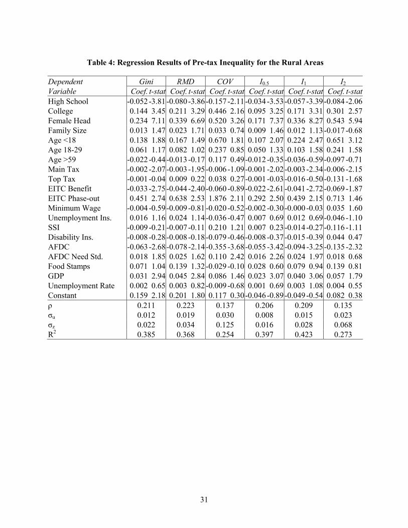
Table 4: Regression Results of Pre-tax Inequality for the Rural Areas

Dependent Gini RMD COV I0.5 I1 I2

Variable Coef. t-stat Coef. t-stat Coef. t-stat Coef. t-stat Coef. t-stat Coef. t-statHigh School -0.052 -3.81 -0.080-3.86 -0.157 -2.11-0.034 -3.53 -0.057 -3.39 -0.084 -2.06College 0.144 3.45 0.211 3.29 0.446 2.16 0.095 3.25 0.171 3.31 0.301 2.57Female Head 0.234 7.11 0.339 6.69 0.520 3.26 0.171 7.37 0.336 8.27 0.543 5.94Family Size 0.013 1.47 0.023 1.71 0.033 0.74 0.009 1.46 0.012 1.13 -0.017 -0.68Age <18 0.138 1.88 0.167 1.49 0.670 1.81 0.107 2.07 0.224 2.47 0.651 3.12Age 18-29 0.061 1.17 0.082 1.02 0.237 0.85 0.050 1.33 0.103 1.58 0.241 1.58Age >59 -0.022 -0.44 -0.013-0.17 0.117 0.49-0.012 -0.35 -0.036 -0.59 -0.097 -0.71Main Tax -0.002 -2.07 -0.003-1.95 -0.006 -1.09-0.001 -2.02 -0.003 -2.34 -0.006 -2.15Top Tax -0.001 -0.04 0.009 0.22 0.038 0.27-0.001 -0.03 -0.016 -0.50 -0.131 -1.68EITC Benefit -0.033 -2.75 -0.044-2.40 -0.060 -0.89-0.022 -2.61 -0.041 -2.72 -0.069 -1.87EITC Phase-out 0.451 2.74 0.638 2.53 1.876 2.11 0.292 2.50 0.439 2.15 0.713 1.46Minimum Wage -0.004 -0.59 -0.009-0.81 -0.020 -0.52-0.002 -0.30 -0.000 -0.03 0.035 1.60Unemployment Ins. 0.016 1.16 0.024 1.14 -0.036 -0.47 0.007 0.69 0.012 0.69 -0.046 -1.10SSI -0.009 -0.21 -0.007-0.11 0.210 1.21 0.007 0.23 -0.014 -0.27 -0.116 -1.11Disability Ins. -0.008 -0.28 -0.008-0.18 -0.079 -0.46-0.008 -0.37 -0.015 -0.39 0.044 0.47AFDC -0.063 -2.68 -0.078-2.14 -0.355 -3.68-0.055 -3.42 -0.094 -3.25 -0.135 -2.32AFDC Need Std. 0.018 1.85 0.025 1.62 0.110 2.42 0.016 2.26 0.024 1.97 0.018 0.68Food Stamps 0.071 1.04 0.139 1.32 -0.029 -0.10 0.028 0.60 0.079 0.94 0.139 0.81GDP 0.031 2.94 0.045 2.84 0.086 1.46 0.023 3.07 0.040 3.06 0.057 1.79Unemployment Rate 0.002 0.65 0.003 0.82 -0.009 -0.68 0.001 0.69 0.003 1.08 0.004 0.55Constant 0.159 2.18 0.201 1.80 0.117 0.30-0.046 -0.89 -0.049 -0.54 0.082 0.38ρ 0.211 0.223 0.137 0.206 0.209 0.135 σu 0.012 0.019 0.030 0.008 0.015 0.023 σz 0.022 0.034 0.125 0.016 0.028 0.068 R2 0.385 0.368 0.254 0.397 0.423 0.273

32

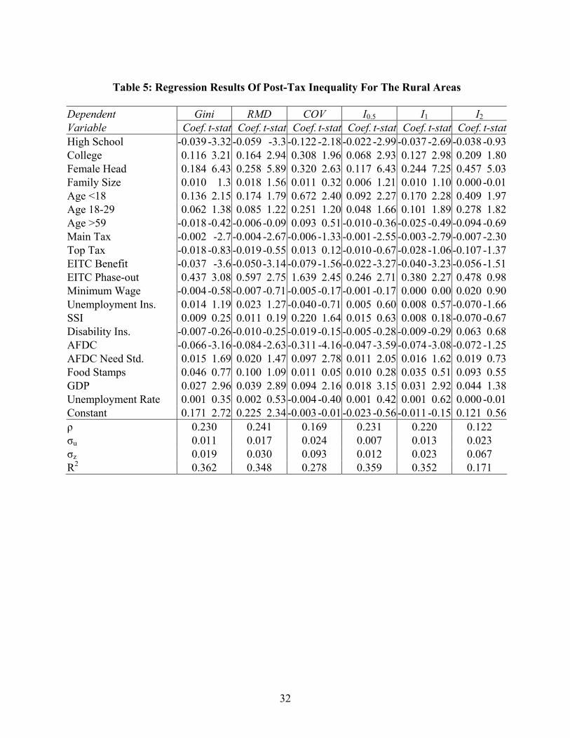
Table 5: Regression Results Of Post-Tax Inequality For The Rural Areas

Dependent Gini RMD COV I0.5 I1 I2

Variable Coef. t-stat Coef. t-stat Coef. t-stat Coef. t-stat Coef. t-stat Coef. t-statHigh School -0.039 -3.32 -0.059 -3.3 -0.122 -2.18-0.022 -2.99 -0.037 -2.69 -0.038 -0.93College 0.116 3.21 0.164 2.94 0.308 1.96 0.068 2.93 0.127 2.98 0.209 1.80Female Head 0.184 6.43 0.258 5.89 0.320 2.63 0.117 6.43 0.244 7.25 0.457 5.03Family Size 0.010 1.3 0.018 1.56 0.011 0.32 0.006 1.21 0.010 1.10 0.000 -0.01Age <18 0.136 2.15 0.174 1.79 0.672 2.40 0.092 2.27 0.170 2.28 0.409 1.97Age 18-29 0.062 1.38 0.085 1.22 0.251 1.20 0.048 1.66 0.101 1.89 0.278 1.82Age >59 -0.018 -0.42 -0.006-0.09 0.093 0.51-0.010 -0.36 -0.025 -0.49 -0.094 -0.69Main Tax -0.002 -2.7 -0.004-2.67 -0.006 -1.33-0.001 -2.55 -0.003 -2.79 -0.007 -2.30Top Tax -0.018 -0.83 -0.019-0.55 0.013 0.12-0.010 -0.67 -0.028 -1.06 -0.107 -1.37EITC Benefit -0.037 -3.6 -0.050-3.14 -0.079 -1.56-0.022 -3.27 -0.040 -3.23 -0.056 -1.51EITC Phase-out 0.437 3.08 0.597 2.75 1.639 2.45 0.246 2.71 0.380 2.27 0.478 0.98Minimum Wage -0.004 -0.58 -0.007-0.71 -0.005 -0.17-0.001 -0.17 0.000 0.00 0.020 0.90Unemployment Ins. 0.014 1.19 0.023 1.27 -0.040 -0.71 0.005 0.60 0.008 0.57 -0.070 -1.66SSI 0.009 0.25 0.011 0.19 0.220 1.64 0.015 0.63 0.008 0.18 -0.070 -0.67Disability Ins. -0.007 -0.26 -0.010-0.25 -0.019 -0.15-0.005 -0.28 -0.009 -0.29 0.063 0.68AFDC -0.066 -3.16 -0.084-2.63 -0.311 -4.16-0.047 -3.59 -0.074 -3.08 -0.072 -1.25AFDC Need Std. 0.015 1.69 0.020 1.47 0.097 2.78 0.011 2.05 0.016 1.62 0.019 0.73Food Stamps 0.046 0.77 0.100 1.09 0.011 0.05 0.010 0.28 0.035 0.51 0.093 0.55GDP 0.027 2.96 0.039 2.89 0.094 2.16 0.018 3.15 0.031 2.92 0.044 1.38Unemployment Rate 0.001 0.35 0.002 0.53 -0.004 -0.40 0.001 0.42 0.001 0.62 0.000 -0.01Constant 0.171 2.72 0.225 2.34 -0.003 -0.01-0.023 -0.56 -0.011 -0.15 0.121 0.56ρ 0.230 0.241 0.169 0.231 0.220 0.122 σu 0.011 0.017 0.024 0.007 0.013 0.023 σz 0.019 0.030 0.093 0.012 0.023 0.067 R2 0.362 0.348 0.278 0.359 0.352 0.171

33

Table 6: Elasticities of Inequality to Policy Variables Gini RMD COV I0.5 I1 I2Urban Pre-tax Main Tax -0.067* -0.047 -0.110 -0.097* -0.111* -0.144* Top Tax -0.021 -0.013 0.008 -0.046 -0.055 -0.054 EITC Benefit -0.024 -0.026 -0.046 -0.056 -0.043 -0.016 EITC Phase-out 0.084* 0.090* 0.241* 0.179* 0.098 -0.050 Minimum Wage 0.135* 0.126* 0.369* 0.282* 0.208* 0.119 AFDC -0.041* -0.041* -0.098* -0.090* -0.080* -0.071* GDP 0.349* 0.378* 0.763* 0.734* 0.605* 0.361* Urban Post-tax Main Tax -0.074* -0.078* -0.127* -0.119* -0.180* -0.196* Top Tax -0.042* -0.036 -0.019 -0.082* -0.078* -0.050 EITC Benefit -0.043* -0.047* -0.063 -0.092* -0.085* -0.085 EITC Phase-out 0.105* 0.110* 0.271* 0.218* 0.141* 0.008 Minimum Wage 0.125* 0.117* 0.351* 0.268* 0.192* 0.151 AFDC -0.045* -0.046* -0.090* -0.094* -0.076* -0.037 GDP 0.340* 0.378* 0.758* 0.756* 0.661* 0.734* Rural Pre-tax Main Tax -0.068* -0.071 -0.094 -0.100* -0.153* -0.151* Top Tax -0.001 0.006 0.018 -0.003 -0.024 -0.098 EITC Benefit -0.071* -0.066* -0.060 -0.140* -0.132* -0.111 EITC Phase-out 0.144* 0.142* 0.277* 0.273* 0.210* 0.169 Minimum Wage -0.030 -0.048 -0.071 -0.045 -0.002 0.198 AFDC -0.045* -0.039* -0.118* -0.115* -0.101* -0.072* GDP 0.332* 0.337* 0.428 0.724* 0.644* 0.454* Rural Post-tax Main Tax -0.075* -0.105* -0.110 -0.124* -0.187* -0.208* Top Tax -0.020 -0.015 0.007 -0.037 -0.052 -0.094 EITC Benefit -0.089* -0.084* -0.092 -0.173* -0.160* -0.106 EITC Phase-out 0.155* 0.147* 0.282* 0.286* 0.223* 0.133 Minimum Wage -0.034 -0.041 -0.021 -0.028 -0.0001 0.133 AFDC -0.052* -0.046* -0.120* -0.122* -0.097* -0.045 GDP 0.321* 0.324* 0.544* 0.703* 0.613* 0.413 * We can reject the hypothesis that the elasticity is zero at the 5% level.

34

Table 7: Welfare Gains or Losses ($) from a 10% Increase in Policy and Female-Head Variables

Urban Rural

I0.5 I1 I2 I0.5 I1 I2

Pre-tax

Main Tax -21.6* -43.2* -129.6* -17.2* -51.6* -103.1*

Top Tax -9.1 -21.7 -42.8 -0.5 -7.3 -59.4

EITC Benefit -18.4 -28.7 -20.5 -35.4* -65.9* -110.9

EITC Phase-out 46.4* 49.9 -52.1 54.5* 81.9* 133.0

Minimum Wage 57.6* 84.2* 97.5 -7.0 -0.1 123.3

AFDC -15.7* -27.5* -50.1* -15.3* -26.2* -37.6*

Post-tax

Main Tax -19.3* -58.0* -135.2* -15.8* -47.5* -110.7*

Top Tax -11.7* -22.4* -30.6 -4.2 -11.7 -44.7

EITC Benefit -22.0* -40.3* -86.1 -32.5* -59.2* -82.8

EITC Phase-out 40.8* 52.5* 6.6 42.2* 65.2* 82.0

Minimum Wage 39.6* 55.5* 95.1 -3.2 0.1 64.8

AFDC -11.8* -19.2* -20.2 -12.0* -19.0* -18.4

* We can reject the hypothesis that these welfare effects are zero at 5% level.

1985 1990 1995

0.40

0.41

0.42

0.43

0.44

0.45

0.46

Gini index of pre-tax income

year

1985 1990 1995

0.36

0.37

0.38

0.39

0.40

0.41

0.42

Gini index of post-tax income

year

Figure 1: Gini Indices of Rural and Urban Areas (urban: solid; rural: dashed)

35

36

FOOTNOTES

1 Moreover, we show that our results are robust to the measure of inequality used. Dalton

(1920) suggested that all common welfare measures would give the same rankings (level) across

countries “in most practical cases.” However, Atkinson (1970) demonstrated that they can give

different rankings. Our claim is different. We show that changes in government policies (and

macroeconomic and aggregate demographic variables) change the rankings of almost all

measures in the same direction.

2 Wu et al. (2003) study the effects of government policies on aggregate U.S. income

distribution.

3 RUPRI (2001) provides state level welfare reform case studies.

4 Throughout this study, we define the central city and suburban areas as urban and the rest non-

metropolitan areas as rural.

5 For details, see “Measuring the Effect of Benefits and Taxes on Income and Poverty: 1979 to

1991,” Current Population Reports Series P-60, No. 182. This series was not included in the

official CPS March Supplement until 1992. The data for the earlier years were obtained from

Unicon Research Corporation (http://www.unicon.com), to whom we are very grateful.

6 For example, for the Atkinson welfare index with ε = 1 (defined below), the average correlation

between the inequality estimates used in this study and those under alternative equivalence scales

is 0.997, 0.939 and 0.989 respectively. Consequently, the estimated coefficients in our

regression analyses are virtually the same for each measure.

7 Our policy impact results are little changed if we use state-level GDP and unemployment rates

rather than federal-level indices. We report the federal-level analysis to avoid circularity in our

regression analyses of income distributions.

37

( ) ( )* 2

0log

y

8 We also examined other inequality measures, such as the standard deviation of the logarithm

of income, y f y dy⎡ ⎤⎣ ⎦∫ , but do not discuss them here to save space. The standard

deviation of the logarithm is almost perfectly correlated with I1.5.

9 The CPS does not cover both rural and urban areas for the entire sample period. For certain

states we have only 3 observations for rural areas over the 17 years of our sample.

Consequently, we use a random-effect model rather than a fixed-effect model, which have short

panel lengths for some states. As a check, we also estimated a fixed-effect model and found that

the results are very close to those of random-effects models.

10 According to the SBTC, the supply of educated workers cannot explain an increase in

inequality and that the main source of the surge of inequality is from demand factors. Studying

the pattern of worker migration across states, Dalh (2002) finds that highly educated workers are

more mobile and migrate to states where the expected return to education is higher. His work

implies that demand, rather than supply, factors are responsible for the positive association

between a larger proportion of highly educated workers and a higher income inequality at state

level, which is consistent with our results.

11 For example, in 1997, 44.3% of the tax filers in urban areas in the CPS March files were in the

main tax bracket while 1.2% of them were in the top tax bracket, compared to 50.7% and 0.5%

for rural areas.