SOIL SCIENCE SOCIETY OF AMERICAJOURNAL

VOL. 45 JULY-AUGUST 1981 No. 4

DIVISION S-l—SOIL PHYSICS

Effect of Field Variability in Soil Hydraulic Properties on Solutions ofUnsaturated Water and Salt i Flows1

DAVID Russo AND ESHEL BRESLER

ABSTRACT

Using actual field variability data and the stochastic approach, effectsof spatial variability of soil hydraulic properties on the predictions ofwater and salt flow distributions, and of correlation structure, areevaluated. The governing water and salt flow equations are solvednumerically using actual field data of soil hydraulic conductivity anddifferential water capacity. These data, which had been obtainedpreviously from measurements made in 30 different locations in a field,were the same as those obtained from a Monte-Carlo simulation thatconsidered the correlations between the parameters of the hydraulicfunctions. Simulated values of pressure head (h), water fluxes (q),wetting front positions (Z,), and solute concentration (c) for each of the30 locations in the field were used to estimate distribution types (normalor log-normal) and its moments, for h, q, Zp and c. The two-pointautocorrelation functions of pressure head, wetting front, and soluteconcentration have been calculated and used to estimate the integralscales oth,Zp and c. Distances in the field in which the horizontal flowcomponents were negligibly small compared with the vertical flowcomponents were calculated and found to be in the order of 10 cm andlarger. Field dispersion of solutes was calculated from the simulated saltdistribution results. Values of field scale dispersivity were estimated tobe larger than the pore scale dispersivity and to increase with soil depth.An "equivalent" uniform porous medium, which was defined at the soilsurface, exists for large infiltration time when a unit hydraulic gradientmay be assumed.

Additional Index Words: hydraulic conductivity, autocorrelationfunction, dispersivity, salinity, leaching.

Russo, D., and E. Bresler. 1981. Effect of field variability in soilhydraulic properties on solutions of unsaturated water and saltflows. Soil Sci. Soc. Am. J. 45:675-681.

'Contribution from the Agric. Res. Organization, the VolcaniCenter, Bet Dagan, Israel, no. 294-E, 1979 series. This researchwas partly supported by a grant from the U.S. - Israel BinationalAgric. Res. and Development Fund (BARD). Received 14 Dec.1979. Approved 12 Mar. 1981.

2Graduate Research Assistant and Soil Physicist, respectively,Division of Soil Physics, ARO, Bet Dagan, Israel.

THE MOST COMMON APPROACH to calculate solute concent-ration, water contents, pressure heads, and fluxes as a

function of time and space has been to model water andsolute transport by using macroscopic quantities which varyin a deterministic manner, obey physical and chemical laws,and are expressed in the form of partial differential equ-ations. To solve these equations it is usually assumed thattheir flow parameters are uniform throughout the entire field(e.g., Bresler, 1973, 1975; Pickens et al., 1979). In reality,however, fields—unlike small laboratory soil columns—areseldom homogeneous, so that their hydraulic propertiesvary from place to place in the field (Nielsen et al, 1973), andflow problems cannot generally be resolved by defining an"equivalent uniform poroous media" (Freeze, 1975).

Being aware of the need to describe the spatial variabilityof field soils characteristics in statistical terms, variousstochastic models have analyzed flow in porous materialusing stochastic parameters rather than deterministic ones(e.g., Warren and Price, 1961; Freeze, 1975; Warrick et al.,1977). A recent contribution to the development of modelswith statistically independent hydraulic parameters andrandom infiltration rates is the work of Dagan and Bresler(1979) and Bresler and Dagan (1979). In this work, theproblem of vertical solute transport caused by steadyinfiltration in unsaturated soils is considered. Our study in afield 0.8 ha in size at Bet Dagan, Israel (Russo and Bresler,1981) showed that soil hydraulic properties are highlyvariable even within a given small field. We also pointed outthat the variations of the properties are not completelydisordered but have structured arrangement with typicaldimensions which must affect the probability distributionsand the correlation distance (characterized by the integralscale) of soil water pressure head, specific flux, salt concent-ration, and wetting depth.

The general objective of this study is therefore to analyzehow and to what extent the inherent spatial variability of thesoil hydraulic properties influence water and salt flowdistributions. Using actual field variability data and thestochastic approach, we will emphasize the impact of spatial

675

676 SOIL SCI. SOC. AM. J., VOL. 45, 1981

correlation structure of the soil hydraulic properties on thesimulated results of water and salt flow. The purpose is alsoto examine the predicted water and salt flow results in termsof their structures and their effects on the utilization of field-measured soil data.

GOVERNING EQUATIONS AND BOUNDARYCONDITIONS

The equation governing nonsteady, one-dimensional,nonhysteretic unsaturateJ water flow in the z (vertical-positive downward) direction of the i-th location in aheterogeneous field is

[1]

Here, t is time, h is soil water pressure head, and K'(h') andC'(h') are the hydraulic conductivity function and differentialwater capacity function, respectively, at the discrete locationi in the field. At the site i the hydraulic conductivity functionis assumed to be

d(c9)' d(qcj

\2p'+2. h<h> [2]

where K^ is the value of K' at soil saturation (h ̂ tiw) at thesite i, h'w is the water entry value of h at i, and /?' is a soilhydraulic parameter characterizing the pore size distri-bution (Russo and Bresler, 1981). To evaluate the functionC'=(dO/dh)' we use the expression

so that

[3]

[4]

where 9is and tfr are the saturated and residual water

contents, respectively, and C'(tf)=Q for Ji'^Ji'w (Russo andBresler, 1981).

The governing equation (Eq. [1]) is supplemented withthe boundary and initial conditions. For the infiltration casethese are

(dh/8z)i = (

ti = ti

z = Z t>0 [5]0 = z = Z t = 0,

where RI is the rain or irrigation intensity, Z is the lowerboundary, and /jj, are predetermined, initial pressure headconditions. Note that in Eq. [5], RI= -[K(dhldz)-Y]whenever RI < Ks.

Numerical solutions of Eq. [1], subject to Eq. [5] for theprofile at location i in the field, are available in the literature(e.g., Neuman et al., 1975; Hanks et al., 1969) from whichwater contents and flow velocities are obtained. These valuescan then be used in the solution to the salt flow equation.

The equation governing transient, vertical piston flow ofan inert (noninteracting) solute at the i-th location in the fieldis

dt dz [6]

in which c is the dimensionless salt concentration and q is thespecific water flux. Expanding Eq. [6] with the use of thecontinuity equation for water (dO/dt)' = — (dq/dz)', we obtain

[7]

The rate of propagation of a given concentration c at a givenlocation i in the field is obtained from Eq. [7] as

[8]' e\z,Note that for those heterogeneous fields in which pore-scaledispersion contributes very little to field-scale dispersion, Eq.[6] through [8] are good approximations (Dagan andBresler, 1979; Bresler and Dagan, 1979) to solute flows.

Solutions of Eq. [8] are possible by the Runge-Kuttamethod, provided that q\z,t) and 9\z,t) are known from thesolution of Eq. [1] and subject to Eq. [5]. The functionsK'Qi1) and (?(#), 0W) which are required for the solutionscan be calculated with the aid of the five hydraulicparameters 6'^ 9^ h^ /?', and K's. Values of these parametersare available for 30 locations (i = 1,2,..., 30) in a field at BetDagan, Israel (Russo and Bresler, 1981), and these values canbe used as input parameters for the solutions. Mean valuesobtained for each of these parameters for the 0- to 90-cmd_epths were #s=0.37, #r=0.08, Kw= -7.4 cm, /?=0.68, andKs=3.7 x 10 -3 cm/sec.

DISTRIBUTION OF THE HYDRAULIC FUNCTIONSThe distribution of the hydraulic function C'(/4 or 8f(ti)

and K'(h') in a heterogeneous field, from measurements ofthe five parameters &„ &„ h^ ft', and K's and Eq. [2] and Eq.[3] or Eq. [4], can be obtained either by Monte-Carlosimulation or by using the actual parameteric field values.The Monte-Carlo method (Hamersley and Handscomb,1964), however, must be combined with the multivariatedistribution function method (Mood and Graybill, 1963).For this, the distribution functions (e.g., normal or log-normal) and their moments for each of the five hydraulicparameters, in addition to correlation coefficients betweenany pairs of parameters, must be provided for the field. Thealternative method is to use the actual values of the fiveparametersxfor each site i of the 30 locations in our field atBet Dagan. These two alternatives should give similar resultsif each of the five hydraulic parameters can be viewed as astationary process. This is demonstrated in Fig. 1, where thesimulated results and the results of 9(h) and K(h) calculatedfrom Eq. [2] and Eq. [3] are almost identical. Only onedepth (60 cm) was chosen for this demonstration, since theresults of the other three depths (0, 30, and 90 cm) are verysimilar. The Monte Carlo technique, used to obtain thesimulated results of 9(h) and K(h), took into account thecorrelations between the hydraulic parameters and a multi-variate normal density function (Mood and Graybill, 1963).To simulate K(h), we considered u^ln Ky u2 = ln /?, andu3 = hw as elements of a vector u which has a trivariate

RUSSO & BRESLER: EFFECT OF FIELD VARIABILITY IN SOIL HYDRAULIC PROPERTIES 677

normal density function with means /jj = —6.45, /i2 = 1.13,and fi3 = — 7.42 cm of water, variances a\ 1 = 0.84, a\2 = 0.75,and 0-33=2.5 cm2 of water; and correlation coefficientsP

212=QA1, p2

3 =0.38, and p23=0.16. Similarly, for 6(h), we

used H j = 0s, u2 = 0r, and u3=ln /J, with means /it = 0.376,/i2 =0.093, ju3= -1.13; variances «7^= 0.0015, ff|2 =0.0012,<T2

3=0.75; and correlation coefficients p22=-.26,

P23 ~ 0-45, an^ Pi 3 = 0.18. In this case we considered hw as anindependent normal variate with mean \i = — 7.42 cm ofwater and variance a2 = 2.50 cm2 of water. Following Freeze(1975), N = 200 random values of ft 6y &„ hw, and Ks weregenerated. Using these parametric values, the functions d(h)and K (h) (/ = 1, 2, ..., N) were calculated from Eq. [2] and [3]for values of h of : 0, -10, -15, -20, -25, -40, -90-,— 120-, — 140-, and — 180-cm of water. The results of meanvalues of 6(h) and K(h)

simulated results of water and salt flows, we do not useMonte-Carlo simulation (in which the values of the para-meters of Eq. [2] through [4] are chosen at random,regardless of their spatial position), but rather used theactual values of the five hydraulic parameters which weremeasured at each of the 30i sites of our field (Russo andBresler, 1981). Thus, for each of the i = 1,2,..., 30 sites of thefield (see Fig. 1 of Russo and Bresler, 1981), Eq [1] and [5]are solved numerically for ti(z, t) and &(z, t) using thenumerical scheme of Hanks et al. (1969). The nonuniformityof the hydraulic functions in the vertical direction has beentaken into account by dividing the soil profile of each site iinto four layers, each of which is characterized by givenvalues of Kj, hj, 6S', 6J, and 0f. The value of K''(z) at theboundary between the layer above z and below z has beencalculated by

i.e. 0= and K= w=^and the interval #+SDe and K + SDk are given in Fig. 1.

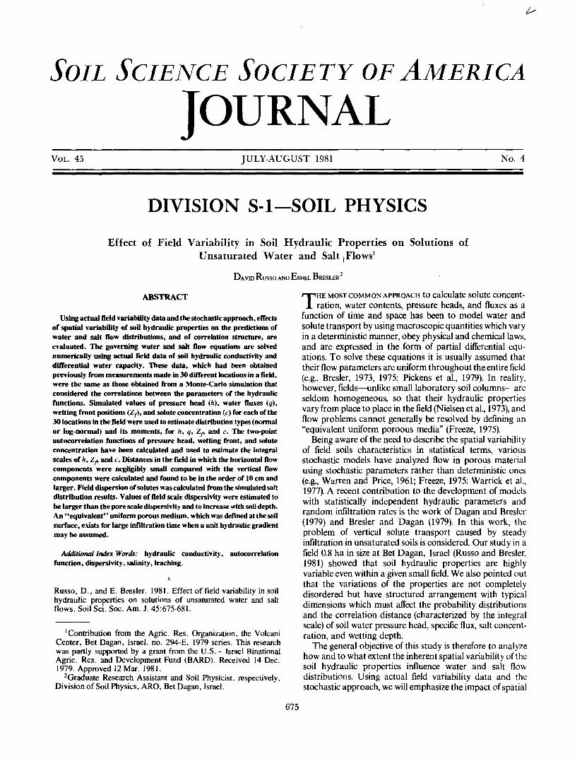
We have also calculated 6(h) and K(h) from EqL[2] and[3] using mean values (for each depth) of #„ #„ Kw K^ and ft.These 9(h) and K(h) functions, which can be said to be"deterministic" functions, are given by the solid lines in Fig.1. It is seen that the mean S(h) and K(h) values areconsistently higher than the deterministic ones. Generally,the disagreement between mean S(h) values and determinis-tic values increases as the value of h decreases.

From the results demonstrated in Fig. 1 and the similarresults for the three additional investigated depths (0., 30,and 90 cm), one can conclude that a Monte-Carlo simu-lation technique can be used to obtain the hydraulic functionCty') and Kty) to be used for the solution of Eq. [1] and [5]for a heterogeneous field soil. In the present study, however,since we analyze the effects of the spatial structure andspatial distribution of the hydraulic functions on the

IOO 150-h(cm H20)

Fig. 1—Water content (0) and hydraulic conductivity (AT), at 60 cmdepth, as a function of soil water pressure head (h), as calculatedfrom Eq. [2] and Eq. [3]. Solid lines were calculated using 8P ?„ jf,h w, and r\. Black and open circles denote mean values calculated bythe Monte-Carlo technique and by using the hydraulic data of the 30locations, respectively. The range mean ± SD is represented by thehorizontal bars and by the dashed lines.

[9]

SIMULATED DISTRIBUTIONS OF PRESSURE HEAD,WATER FLUX, WETTING FRONT, AND SOLUTE

CONCENTRATIONValues of hl(z, t), q'(z, t), c'(z, t), and wetting front positions,

Z/(t), were computed for each site i of the 30 locations inthe field, with deterministic values of h0= —1022 cm ofwater, hmax=0, RI = 1.5 cm/hour, and with four layers of 30-cm depth each. The computations were carried out withAz=2 cm to a depth of Z = 120 cm and with Atmin = 0.024hour for 20 hours of continuous, constant RI.

Soil Water Pressure Head hMean values of

30

h=

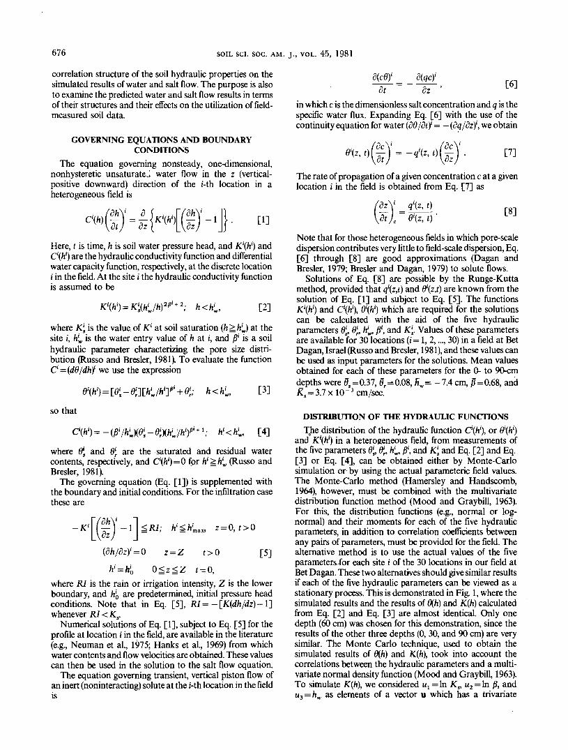
as a function of depth for four infiltration times are given ona semi-log scale in Fig. 2. The figure shows that the spatialvariability of h, as indicated by the coefficient of variationC.V.= SD//I increases as the mean depth of the wetting frontis approached. The trend that C.V.->0 as z-»Z is aconsequence of the fact that the initial conditions aredeterministic, i.e., below the wetting front h is assumed to beequal to h0 throughout the entire field. Also, values of C.V. atthe soil surface are relatively low (<0.30) because theapplication rate RI is deterministic with C.V. = 0. The valuesof C.V. in the transmission zone decrease with time andapproach a constant value of C.V. = 0.24, while C.V. near thewetting front increases with time. The spatial distribution ofh over the field, as inferred from /2 analysis, is generally log-normal near the wetting front and normal in the transmis-sion zone.

Vertical Water Flux qVertical water fluxes at each site i were calculated from

q'(z, t)= -Kty^z, t)][G'(z, 0+1], where the vertical pre-ssure head gradient G' = (dh/dz)' was estimated from the firstderivative of cubic splines. The results show that meanvertical water flux

678 SOIL SCI. SOC. AM. J., VOL. 45, 1981

h ( c m H20)-10* -10'

100-

Fig. 2—Calculated soil water pressure head (h) as a function of depth (z)for four different infiltration times. Solid curves, black circles, anddashed curves represent the same as in Fig. 1. Note that point z=0,indicated by the arrows, is shifted downwards; the data aretranslated accordingly along the z-axis.

q(z, 0= £ q'(z, 0/30i - l

in the transmission zone increases with time and decreaseswith depth. As for the variability of q, it was found thatC.V.q=SD/q increases as the mean wetting front is ap-proached. Again CN.q at the top decreased with time andapproached a constant value of 0.42. The distribution of q asinferred from %2 analysis for the main flow domain isgenerally log-normal (i.e., log q(z, t); N\jj.logq(z r), ff,og^2i „]).

Location of the Wetting Fronts Zf

The wetting front positions Z^t) is defined (Mein andFarrell, 1974) as

Z>(f)=

where 0'0 and 6'w are water contents calculate from Eq. [3] forh'0 and /i'(0, t), respectively. For each site i at a given time t,values of z'(0, t) were smoothed before the integral in Eq. [10]

was numerically evaluated. Here again we inferred from yfanalysis that the spatial distribution of Zfi) is approxi-mately log-normal.

Salt Concentration cSalt concentration propagation from the soil surface

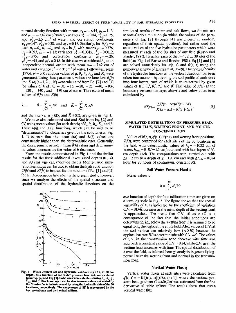
(z=0) to any depth z and in each site i in the field wascalculated from Eq. [8], using q\z, t) and 0'(z, t) obtainedfrom the solution of Eq. [1] and Eq. [5]. For convenienceand generality we considered a deterministic dimensionlessconcentration c = l at z = 0 for all £>0 and initial zeroconcentration throughout the entire field (i.e., semi-infinitecase: c = l, z=0, t>Q; c=0, z^O, t=0). Average saltconcentration distribution in our heterogeneous field isobtained by applying a deterministic uniform recharge (RI)on the soil surface. Here, average concentration over theentire field c(z, t) was calculated by counting the fraction ofsites of the 30 sites in the field through which the saltconcentration front, separating the zone where c = 1 fromthe zone where c=0, has been passed the depth z in time (.These values of c (Fig. 3) represent precisely the ratio for agiven t at a fixed z between the area in the field for which c = 1and the total area. The simulated results demonstrated inFig. 3 are the basis of application of water and salt flowmodels to leaching of salts in heterogeneous field soils. Fromthe simulated results of Fig. 3, one can obtain the length oftime for the leaching process to be complete to a given depthand for a given portion of the entire field. The amount ofwater needed for the same process is calculated simply bymultiplying the appropriate time by RI since, in our case,RI<KS' at any discrete location i. For example, 50% of thefield has been leached to a depth of 25 cm after 4.2 hours ofleaching at a rate of 1.5 cm/hour. This time is equivalent to6.3 cm of water. At the same time and water quantity, only14% of the field has been leached to 35 cm. Similarly, theleaching process is completed throughout the entire field to adepth of 35 cm only after about 11 hours of irrigation and theamount of water needed for this complete process is as muchas 16.5 cm.

CORRELATION DISTANCES OF PRESSURE HEAD,WETTING FRONT, AND SALT CONCENTRATIONSThe spatial variability of each of the five parameters, hw 9^

6P /?, and Ks of Eq. [2] through [4] (the input parameters tothe solution of Eq. [1] and [5]), has a structure that is

I.U

0.8

0.6

0.4

0.2

0.0

n 9o..(

I I 1 ! 1 1 — 1 ———— i ————

- -

-

~

* » • " • « * *'

1 1 1 1 *l 1 1 1) 20 40 60 80

1

-

-

> m

1100

Fig. 3—"Average" dimensionless concentration as a function of in-filtration time (t) for nine soil depths as indicated by the numberslabeling the curves.

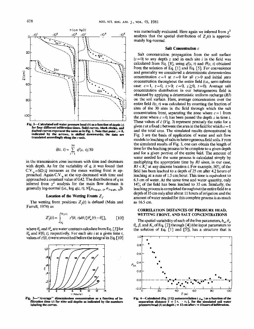
T(m)Fig. 4—Calculated (Eq. [11]) autocorrelation ( pM.) as a function of the

separation distance T = | r, — r2 \, for the simulated soil waterpressure head (h) at depth z = 12 cm after 1 = 4 hours of infiltration.

RUSSO & BRESLER: EFFECT OF FIELD VARIABILITY IN SOIL HYDRAULIC PROPERTIES 679

—1V1 i = 1 i = 1

1 M

5 Z-1211/2

»W| }1 M

s Z1/2

characterized by a correlation distance (Russo and Bresler,1981). The output variables of Eq. [1], [5], and [8], such asthe pressure head (h), the wetting front position (Zf\ and thesalt concentration (c), must also have correlation distances.The correlation distance of any output variable u (where u ish, Zf, or c) is evaluated by first calculating the two-pointautocorrelation function pj^) of u, and then calculating theintegral scale J of u. The two-point autocorrelation functionis calculated from the simulated values of u at each of the 30sites in the field (Russo and Bresler, 1981) by using Eq. [11].Here M = M(x) is the number of pairs of data pointsseparated by the distance i. As the distance between the sitesis not regular (Russo and Bresler, 1981, Fig. 1), the numberM varies and may be determined for each t as follows. Allpairs of data points separated by a distance T=0-2 m, 2-4 m,..., 98-100 m, were grouped to distance classes having M > 2pairs of points in each class. The values of T used in the pj^)functions were the midpoint values of i i.e., T = 1, 3,..., 99 mfor the classes 0-2, 2-4, ..., 98-100 m, respectively. Anexample of pm(r) function calculated from Eq. [11] for thesimulated soil-water pressure head (u=h) at depth of z = 12cm after 4 hours of infiltration is given in Fig. 4.

The essential features of the dependence of pm upon T areexpressed quantitatively by the integral scale (J) and themicroscale (/). The integral scale can be interpreted as thelargest average distance T=| r 2 — r l \ for which the values of uat r2 and rl are correlated. The microscale is the averagedistance for which the correlation coefficient does not differstatistically from 1. The micro- and integral scales can beconsidered as characteristic field lengths which are de-termined from the autocorrelation functions. Assuming thateach of the output variables, u can be viewed as two-dimensional isotropic and stationary stochastic processes, Jand / of u can be calculated by

and

J,.=

[12]

[13]

Note that in a one-dimensional process, like a time series, theintegral scale is just the integral of the autocorrelationfunction. Values of the integral scale of h, Zf, and c wereestimated from Eq. [13] using numerical evaluation of theintegral in Eq. [13] for the whole domain of pm(t). Thecalculations were carried out for each six soil depths: 0-20,0-32, 0-40, 0-48, 0-54, and 0-64 cm (with increments ofAz=4 cm), for the respective six infiltration times, t=1,2,3,4, 5, and 6 hours. Note that the values of Ju calculated fromEq. [13] are only approximations representing the magni-tude of Ju rather than its exact value. This is so becausescattered data points (Fig. 4) were used for numericalevaluation of the integral in Eq. [13]. It was impossible,however, to calculate lu from Eq. [12] because of difficulties

in estimating [d2pm/dr1'\r=0, due to insufficient points in theregion close to T=0. Note that if sufficient amount of datawere collected close to r = 0, we would have been able toestimate /„ from Eq. [12].

Pressure Head /z-The integral scale and C.V. of thesimulated h in the transmission zone were calculated to be 17meters and 0.24, respectively. These values are very similar tothe equivalent values of /iw. Smallest values of Jh were foundat the wetting fronts where at all times Jh = 6 meters, andC.V.h = 1.0. Intermediate values of Jh were calculated for thetransition zone between the wetting front and the transmis-sion zone.

Wetting Front Position Z^-Data of the integral scale,average depth, and C.V. (standard deviation divided byaverage depth) of the simulated wetting front position (Eq.[10]) are given in Table 1 for seven discrete infiltration times.The increase in the values of Jz,with time is associated with

zf .M. 11W 411WJ.WM.UW ill H»W IMIMWkJ W« J 7 *"

the decrease in the values of C.V.Correlation Distance of c—The integral scale of the

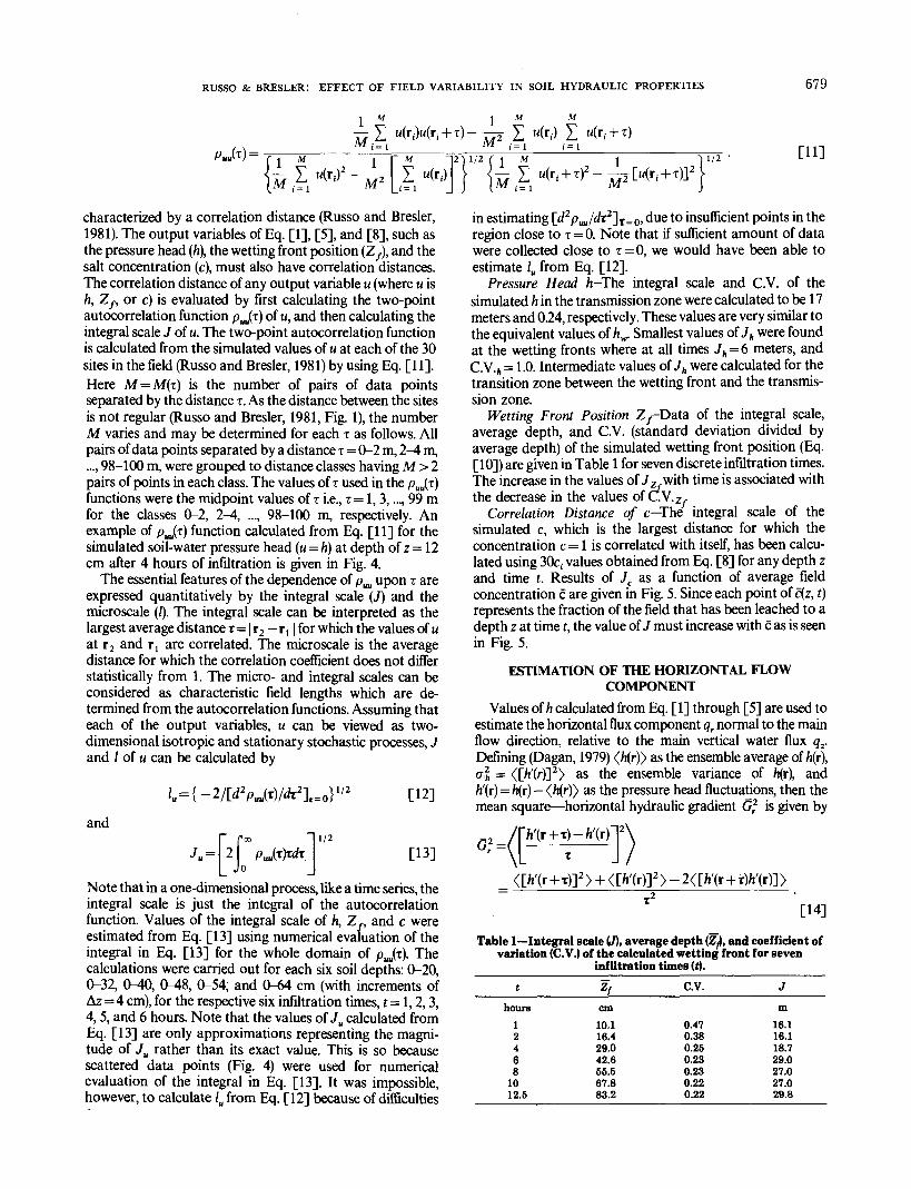
simulated c, which is the largest distance for which theconcentration c = 1 is correlated with itself, has been calcu-lated using 30c; values obtained from Eq. [8] for any depth zand time t. Results of Jc as a function of average fieldconcentration c are given in Fig. 5. Since each point of c(z, t)represents the fraction of the field that has been leached to adepth z at time t, the value of J must increase with c as is seenin Fig. 5.

ESTIMATION OF THE HORIZONTAL FLOWCOMPONENT

Values of h calculated from Eq. [1] through [5] are used toestimate the horizontal flux component qr normal to the mainflow direction, relative to the main vertical water flux qfDefining (Dagan, 1979) </i(r)> as the ensemble average of/z(r),er2, = <rjj'(r)]2> as the ensemble variance of h(t), and/i'(r)=/z(r)-<Ji(r)> as the pressure head fluctuations, then themean square—horizontal hydraulic gradient Gr

2 is given by

[14]

Table 1—Integral scale (7), average depth (Zfl, and coefficient ofvariation (C.V.) of the calculated wetting front for seven

infiltration tunes (t).t

hours12468

1012.5

Zfcm10.116.429.042.655.567.883.2

C.V.

0.470.380.250.230.230.220.22

J

m16.116.118.729.027.027.029.8

680 SOIL SCI. SOC. AM. J., VOL. 45, 1981

60

50

30-

20-

10-

60

.2 .4 .6 .8 1.0

C(z, t )Fig. 5—Integral scale of solute concentration as a function of the

"average concentration (f). Black circles denote calculated valuesfor different combinations of infiltration time and soil depths.

From the definition of the autocorrelation functionPwi(T) = </j'(rMr + T)>/<7,,2 (see Eq. [1.32] in Lumley andPanofsky, 1964) and since in a stationary process

[15]

The autocorrelation functions for the output variable h ascalculated from Eq. [11] were fitted to the quadraticequation in the form pw,(T) = l+ar + br2 (a, b<0), whichupon substitution into Eq. [15] yields

Gr(z, t |T) = z, r)[-at-&T2)]1/2/T. [16]

Equation [16] with the best fitted values of a= -0.03 andb= -0.0002 (with r2=0.98 obtained for the transmissionzone) can be used to estimate the distance T in which thehorizontal flux component is negligibly small comparedwith the vertical flux component (i.e., qr«:<jz). Note that ifsufficient amounts of data were collected close to r=0 wewould have been able to estimate lh from Eq. [12] and tocalculate average horizontal gradient GP from Eq. (1.35) ofLumley and Panofsky (1964):

[17]

[18]

Gr(z, t) = y2SD,(2, t)/lh(z, t),

and mean horizontal flux, (qr), by

qr(z, t)=-K[E(z, t)-]-G,(z, t [

Here K is calculated from Eq. [2], with average values (for agiven depth) of K^ hw and ft, and assuming isotropy.

Computations of Gr(z, t|t) (Eq. [16]) and qr(z, t|r) (Eq.[18]) were carried out for each of the soil depths 0-20, 0-32,0-40, 0-48, 0-54, and 0-64, cm (with increments of Az=4cm) for the respective six infiltration times, t = 1, 2, 3,_4, 5, and6 hours. Results show that the horizontal values of Gr and q^for T >0.1 meter in the transmission zone, are smaller than3 x 10 ~2 cm /cm and 3.5 x 10 ~ 2 cm /hour respectively. Closeto the wetting front, values of Gr increase with depth (inagreement with the increase in the values of SDJ while valuesof qr decrease with depth [in agreement with the decrease inthe values of K(fi)]. At mean depths of the wetting front of 10,20, 26, 32, 39, and 44 cm for t = 1, 2, 3, 4, 5, and 6 hours,

40

20

f-II .

6 10 20 30 40 50z (cm)

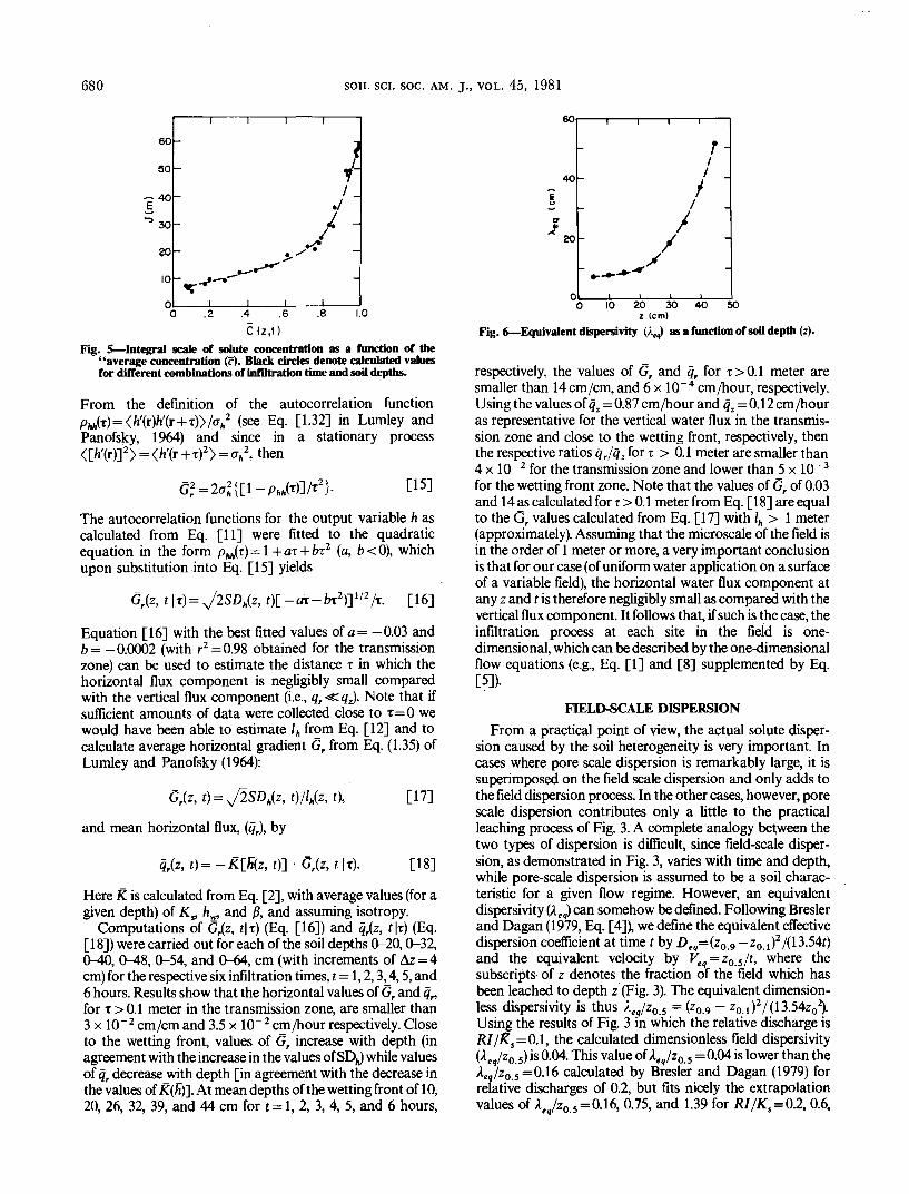
Fig. 6—Equivalent dispersivity (Ae,) as a function of soil depth (z).

respectively, the values of Gr and qr for T>0.1 meter aresmaller than 14 cm/cm, and 6 x 10~4 cm/hour, respectively.Using the values of qz = 0.87 cm/hour and qz = 0.12 cm /houras representative for the vertical water flux in the transmis-sion zone and close to the wetting front, respectively, thenthe respective ratios qr/q, for T > 0.1 meter are smaller than4 x 10"2 for the transmission zone and lower than^ x 10"3

for the wetting front zone. Note that the values of Gr of 0.03and 14 as calculated for T > 0.1 meter from Eq. [18] are equalto the Gr values calculated from Eq. [17] with lh > 1 meter(approximately). Assuming that the microscale of the field isin the order of 1 meter or more, a very important conclusionis that for our case (of uniform water application on a surfaceof a variable field), the horizontal water flux component atany z and t is therefore negligibly small as compared with thevertical flux component. It follows that, if such is the case, theinfiltration process at each site in the field is one-dimensional, which can be described by the one-dimensionalflow equations (e.g., Eq. [1] and [8] supplemented by Eq.[5]).

FIELD-SCALE DISPERSIONFrom a practical point of view, the actual solute disper-

sion caused by the soil heterogeneity is very important. Incases where pore scale dispersion is remarkably large, it issuperimposed on the field scale dispersion and only adds tothe field dispersion process. In the other cases, however, porescale dispersion contributes only a little to the practicalleaching process of Fig. 3. A complete analogy between thetwo types of dispersion is difficult, since field-scale disper-sion, as demonstrated in Fig. 3, varies with time and depth,while pore-scale dispersion is assumed to be a soil charac-teristic for a given flow regime. However, an equivalentdispersivity (Ae,) can somehow be defined. Following Breslerand Dagan (1979, Eq. [4]), we define the equivalent effectivedispersion coefficient at time t by De^(zog—zol)2/(l3.54t)and the equivalent velocity by Fe,=z05/t, where thesubscripts of z denotes the fraction of the field which hasbeen leached to depth z (Fig. 3). The equivalent dimension-less dispersivity is thus Ae,/z0 5 = (z0 9 — z0 1)2/(13.54z0

2).Using the results of Fig. 3 in which the relative discharge isR//KS=0.1, the calculated dimensionless field dispersivity(Ae,/z0.5) is 0.04. This value of Ae,/z0 5 =0.04 is lower than thele,/Zp.5=0.16 calculated by Bresler and Dagan (1979) forrelative discharges of 0.2, but fits nicely the extrapolationvalues of A /z0.5=0.16, 0.75, and 1.39 for K//KS=0.2, 0.6,

RUSSO & BRESLER: EFFECT OF FIELD VARIABILITY IN SOIL HYDRAULIC PROPERTIES 681

and 1.0, respectively. This inverse relationship between thedimensionless field dispersivity and the relative discharge fora given spatial variability of soil hydraulic properties havebeen previously reported by Bresler and Dagan (1979). Theeffect of ponding areas has also been discussed. It isinteresting to note here that even when RI/KS is very low sothat ponding conditions are very unlikely and dimensionlessfield dispersivity is quite low, the applicability of fielddispersion as is clearly seen in Fig. 3 is, in practice, moreimportant than the pore-scale dispersion in a homogeneousfield. It can be concluded that field-scale dispersion becomesmore important relative to pore-scale dispersion of auniform soil column as the field becomes more variable andas the discharge rate is larger, relative to the field-average—saturated hydraulic conductivity.

An additional possibility of calculating equivalent field-scale dispersivity is by considering the results of Fig. 3 asbreakthrough data and fitting them to a well-knownmiscible displacement solution. The data of Xeq given in Fig.6 were thus calculated with average velocity, equivalent topore water velocity, averaged over time and depth, throug-hout the entire 30 field sites. The results of k^ as a function ofdepth (Fig. 6) confirm the high significance of field-scaledispersion.

EQUIVALENT UNIFORM POROUS MEDIUMIn the traditional, deterministic water flow modeling, one

assumes that it is possible to define a fictitious, uniformporous medium which represents the actual nonuniformmedium and acts as an "equivalent" uniform porousmedium. According to Freeze (1975), equivalence impliesthat mean value of a soil variable (such as the head, h) at anyz and t, as determined from it probability distribution (whichin turn is obtained from a stochastic solution to a boundaryvalue problem), must equal the single value at the same point(z, t) provided from a single "deterministic" solution, carriedout with property values which are equal to some constantsderived from their probability distribution.

To test whether it is possible to select a fictitious porousmedium for our field that satisfies Freeze's definition, adeterministic solution of Eq. [1], subject to Eq. [5], wascarried out. The input hydraulic functions, K(h), and C(h\that were used in this solution were given by Eq. [2] and Eq.[4] with mean values (for each soil layer) of Ks, Kw, fi, Bs, andBr, and with the same values of Armin, Az, h0, /imax, Z, and RIas before.

The results for h of this deterministic run are given by thesolid curves in Fig. 2. The differences between meanstochastic values of h (black circles) and the deterministicvalues are relatively small at the upper part of the wettedzone. Near the wetting front, however, the differences arerelatively large. It seems, therefore, that in the case of a one-dimensional, nonsteady infiltration into a nonuniform soil,an equivalent uniform porous medium cannot be definedsimply by finding mean values of the parameters of Eq. [2]and Eq. [4].

However, at the soil surface for large t where a unithydraulic gradient may be assumed, an equivalent uniformporous medium (as defined by Freeze, 1975) generally exists.This is so because deterministic h values at z = 0 and f-»oo,h(0, oo), calculated using mean values of Kff fiw, and /? is

usually equal to the averageN

h(Q, oo) = £ h,(0, oo)/Ni = l

as calculated by the Darcy's equation with a unit hydraulicgradient, i.e.,

ht(Q, oo) = hU K*-RI

/i,.(0, oo) = /C(Ki/R/)1/(2"i + 2), Kls>RI.

It should be emphasized here that as only 30 simulationswere used to evaluate the spatial distribution of h(z, t}, theconclusions regarding equivalent porous medium should notbe considered as definitive, and further investigation of thisimportant topic is warranted.

ACKNOWLEDGMENTS

The authors are grateful to Gideon Dagan for his constructivesuggestions during this study.