Efficient Reverse k-Nearest Neighbors Retrieval with Local kNN-Distance Estimation

Mike Lin

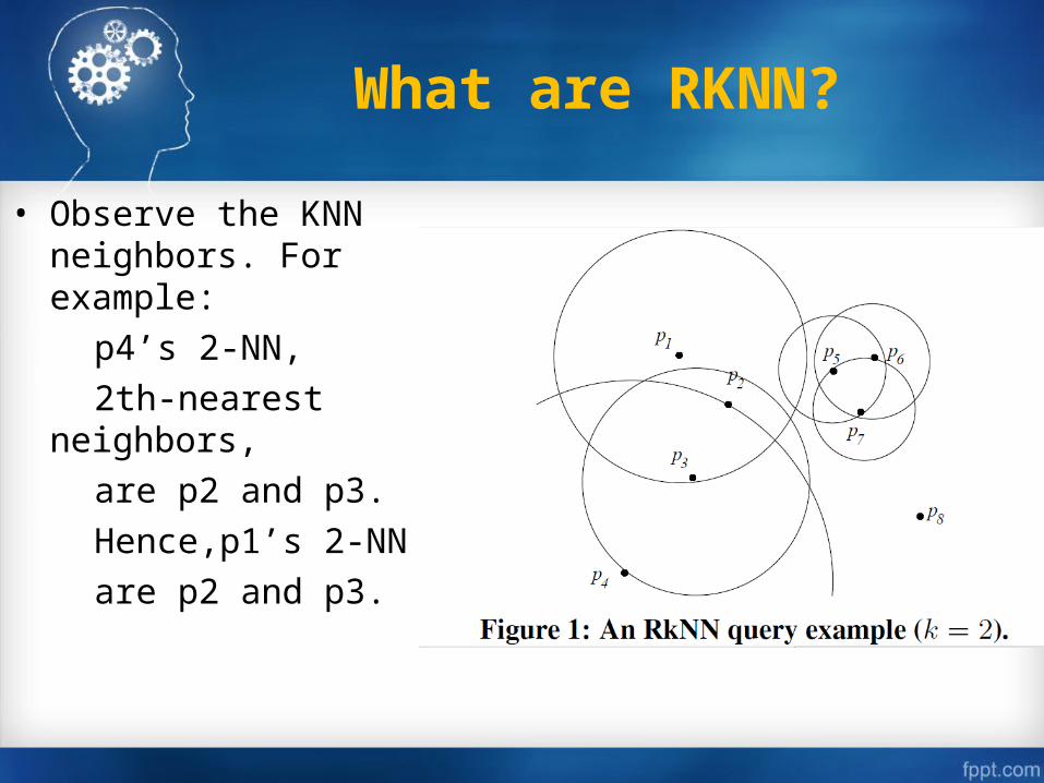
• Observe the KNN neighbors. For example:

p4’s 2-NN,

2th-nearest neighbors,

are p2 and p3.

Hence,p1’s 2-NN

are p2 and p3.

What are RKNN?

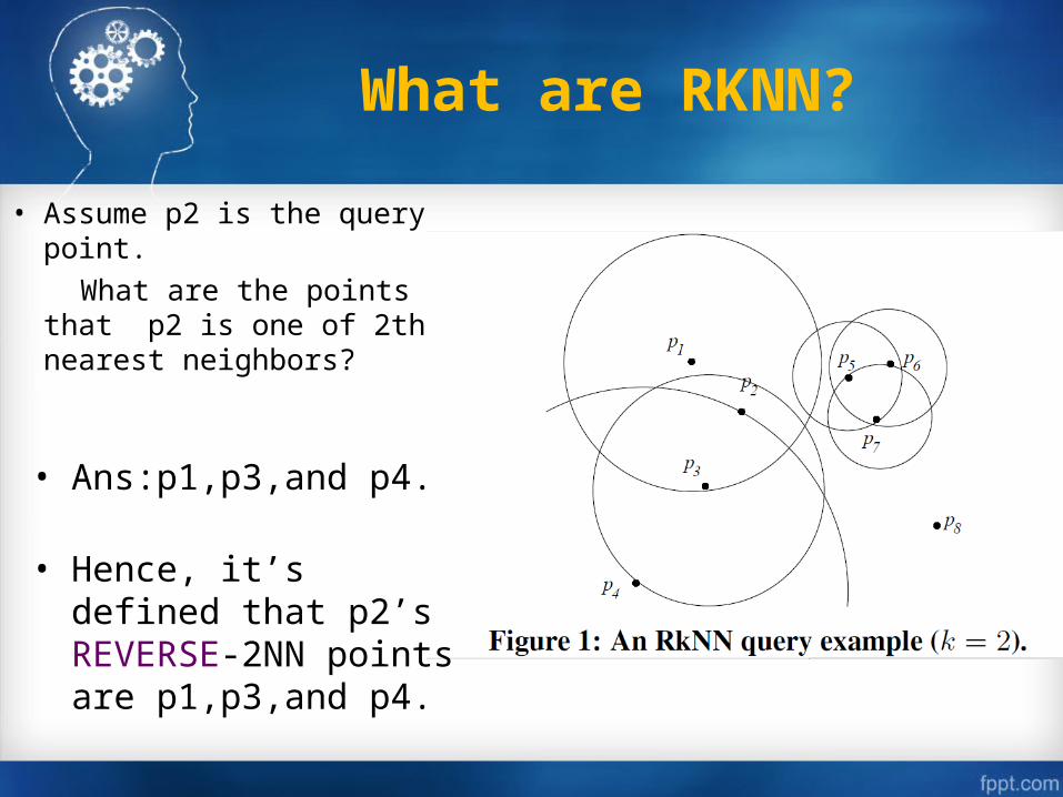
• Assume p2 is the query point.

What are the points that p2 is one of 2th-nearest neighbors?

What are RKNN?

• Ans:p1,p3,and p4.

• Hence, it’s defined that

p2’s REVERSE-2NN points are p1,p3,and p4.

How to do RNN query?

• The various methods have been designed for RNN queries (i.e.,RkNN queries when k = 1).

• In two categories:

• pre-computation methods

• space pruning methods

Pre-computation methods

• With Pre-computation methods pre-compute and store the nearest neighbor information of each point in a dataset in index structures, i.e., the RNN-tree and the Rdnn-tree.

• However, the drawback of pre-computation methods is that they cannot answer an RkNN query unless the corresponding k-nearest neighbor information is available.

Space pruning methods

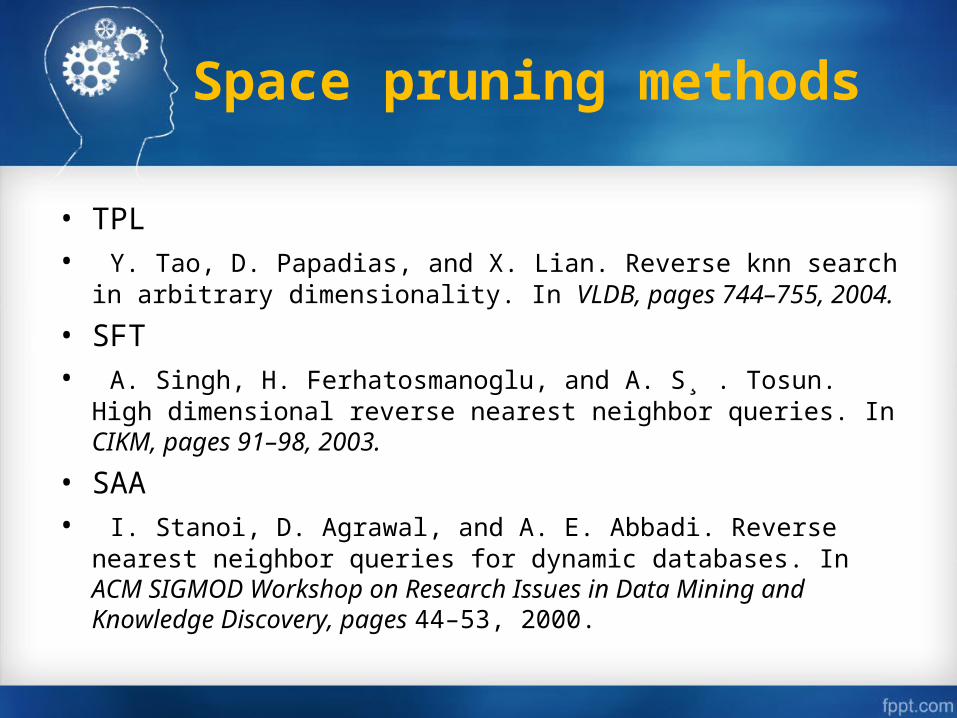
• TPL • Y. Tao, D. Papadias, and X. Lian. Reverse knn search in arbitrary

dimensionality. In VLDB, pages 744–755, 2004.

• SFT • A. Singh, H. Ferhatosmanoglu, and A. S¸ . Tosun. High

dimensional reverse nearest neighbor queries. In CIKM, pages 91–98, 2003.

• SAA • I. Stanoi, D. Agrawal, and A. E. Abbadi. Reverse nearest neighbor

queries for dynamic databases. In ACM SIGMOD Workshop on Research Issues in Data Mining and Knowledge Discovery, pages 44–53, 2000.

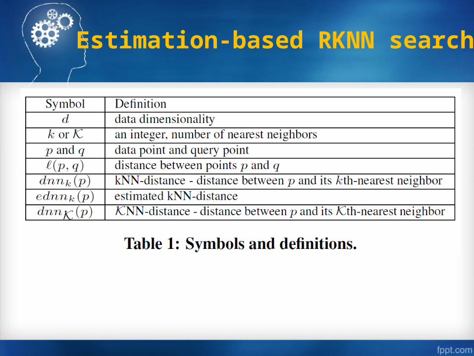
Estimation-based RKNN search

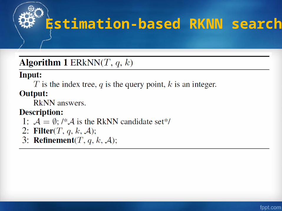
Estimation-based RKNN search

Algorithm 1

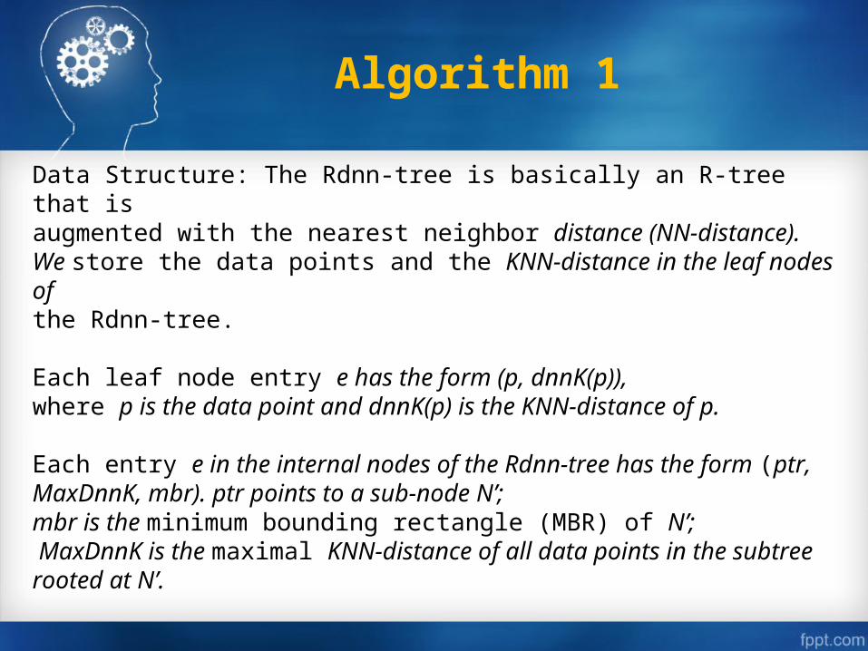
Data Structure: The Rdnn-tree is basically an R-tree that isaugmented with the nearest neighbor distance (NN-distance). We store the data points and the KNN-distance in the leaf nodes ofthe Rdnn-tree.

Each leaf node entry e has the form (p, dnnK(p)),where p is the data point and dnnK(p) is the KNN-distance of p.

Each entry e in the internal nodes of the Rdnn-tree has the form (ptr, MaxDnnK, mbr). ptr points to a sub-node N’; mbr is the minimum bounding rectangle (MBR) of N’; MaxDnnK is the maximal KNN-distance of all data points in the subtree rooted at N’.

Estimation-based RKNN search

Algorithm 2

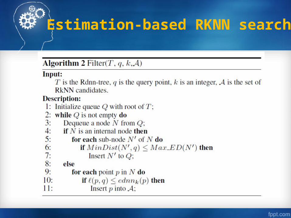
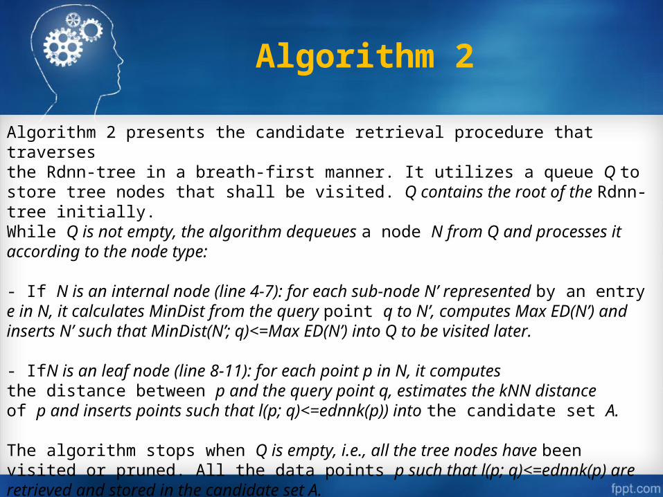
Algorithm 2 presents the candidate retrieval procedure that traversesthe Rdnn-tree in a breath-first manner. It utilizes a queue Q to store tree nodes that shall be visited. Q contains the root of the Rdnn-tree initially. While Q is not empty, the algorithm dequeues a node N from Q and processes it according to the node type:

- If N is an internal node (line 4-7): for each sub-node N’ represented by an entry e in N, it calculates MinDist from the query point q to N’, computes Max ED(N’) and inserts N’ such that MinDist(N’; q)<=Max ED(N’) into Q to be visited later.

- IfN is an leaf node (line 8-11): for each point p in N, it computesthe distance between p and the query point q, estimates the kNN distanceof p and inserts points such that l(p; q)<=ednnk(p)) into the candidate set A.

The algorithm stops when Q is empty, i.e., all the tree nodes have been visited or pruned. All the data points p such that l(p; q)<=ednnk(p) are retrieved and stored in the candidate set A.

Algorithm 2 complexity

The filter procedure of ERkNN is equal to the point enclosurequery, so its complexity is O(logN) , where N is the numberof data points.

Estimation-based RKNN search

Algorithm 3

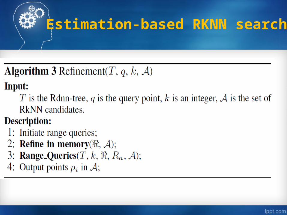
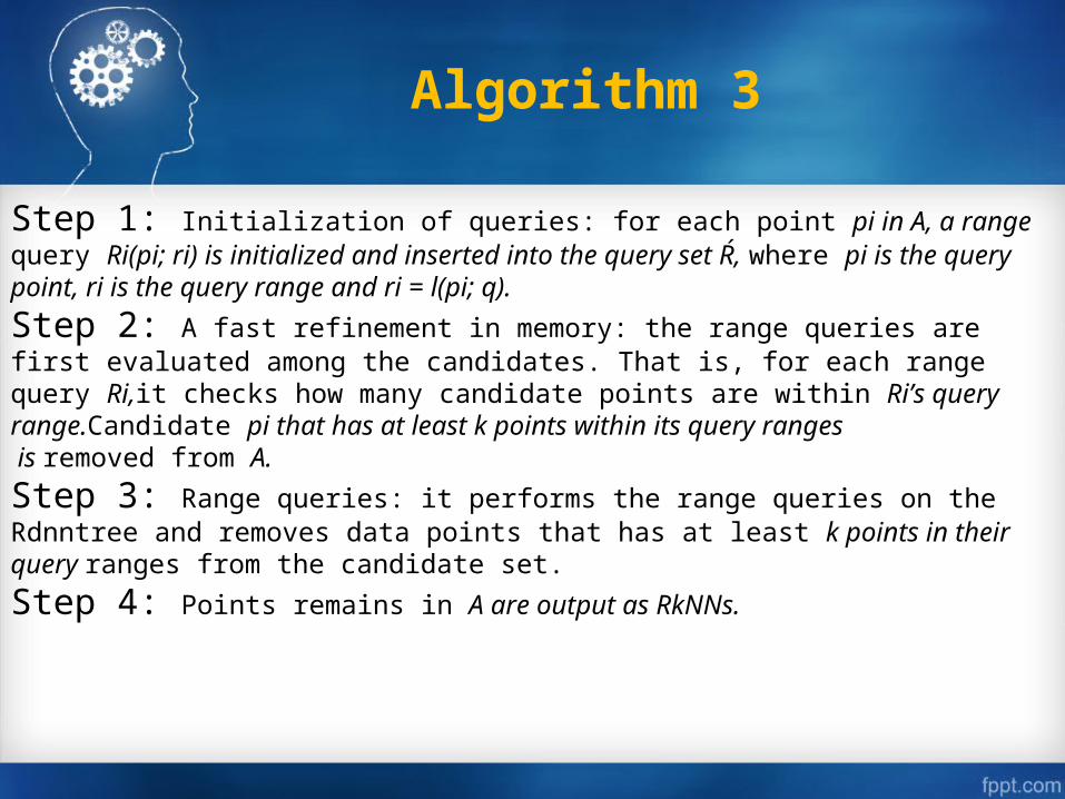
Step 1: Initialization of queries: for each point pi in A, a range query Ri(pi; ri) is initialized and inserted into the query set Ŕ, where pi is the query point, ri is the query range and ri = l(pi; q).

Step 2: A fast refinement in memory: the range queries are first evaluated among the candidates. That is, for each range query Ri,it checks how many candidate points are within Ri’s query range.Candidate pi that has at least k points within its query ranges is removed from A.

Step 3: Range queries: it performs the range queries on the Rdnntree and removes data points that has at least k points in their query ranges from the candidate set.

Step 4: Points remains in A are output as RkNNs.

Algorithm 3

Steps 1-2 and 4 are straightforward. Step 3 dominates the cost incurred in the refinement procedure. In order to reduce both I/O and CPU cost, we apply the aggregation strategy in this step. The basic idea is to first compute an aggregated range query Ra(pa; ra) before carrying out the individual range queries. The query rangeof Ra, which is centered at pa and of radius ra, covers the search ranges of all Ri in Ŕ.

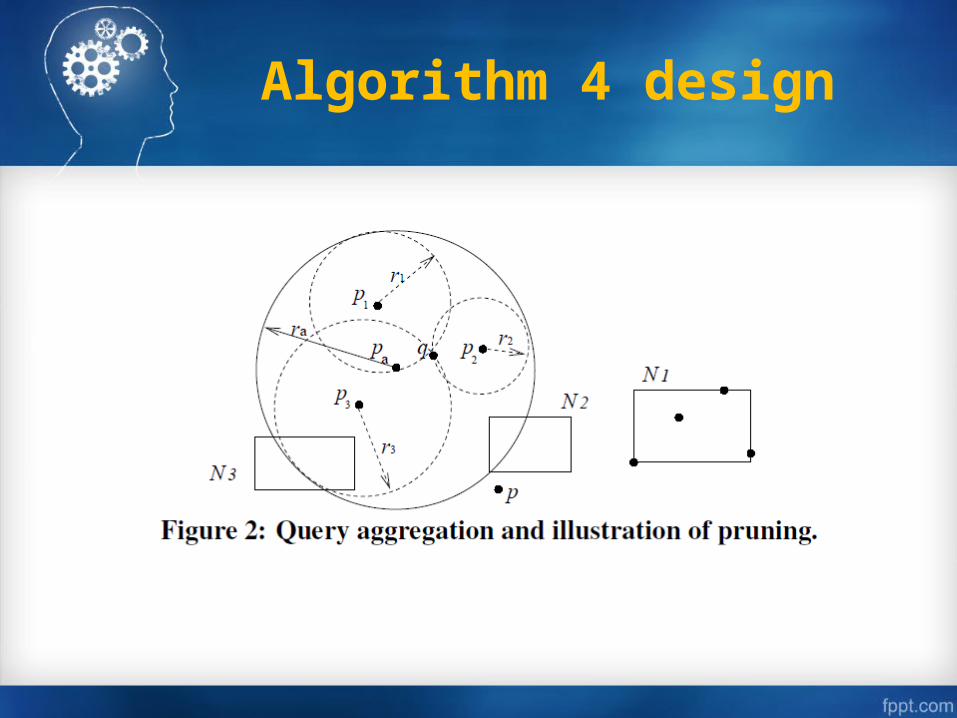
Figure 2 gives an example. There are three candidates p1, p2 and p3. The dashed circles are their query ranges.

The solid circle is the aggregated query Ra. The computation query sphere of Ra is corresponding to the minimum enclosing ball problems whose complexity is lower bounded by O(|A|).

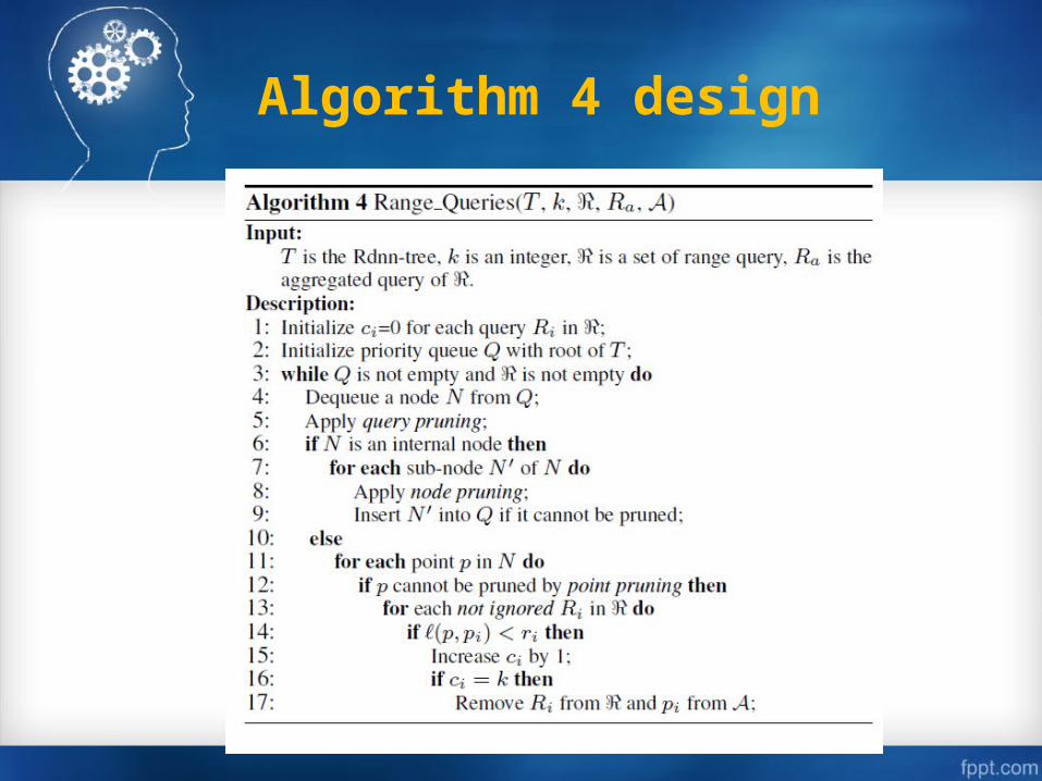
Algorithm 4 design

Algorithm 4 design

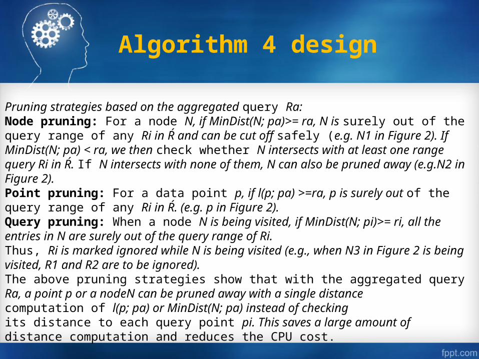
Pruning strategies based on the aggregated query Ra:Node pruning: For a node N, if MinDist(N; pa)>= ra, N is surely out of the query range of any Ri in Ŕ and can be cut off safely (e.g. N1 in Figure 2). If MinDist(N; pa) < ra, we then check whether N intersects with at least one range query Ri in Ŕ. If N intersects with none of them, N can also be pruned away (e.g.N2 in Figure 2).Point pruning: For a data point p, if l(p; pa) >=ra, p is surely out of the query range of any Ri in Ŕ. (e.g. p in Figure 2). Query pruning: When a node N is being visited, if MinDist(N; pi)>= ri, all the entries in N are surely out of the query range of Ri.Thus, Ri is marked ignored while N is being visited (e.g., when N3 in Figure 2 is being visited, R1 and R2 are to be ignored).The above pruning strategies show that with the aggregated queryRa, a point p or a nodeN can be pruned away with a single distancecomputation of l(p; pa) or MinDist(N; pa) instead of checkingits distance to each query point pi. This saves a large amount ofdistance computation and reduces the CPU cost.

Algorithm 4 design

Algorithm 4 design

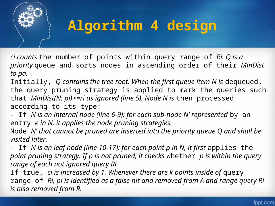
ci counts the number of points within query range of Ri. Q is a priority queue and sorts nodes in ascending order of their MinDist to pa.Initially, Q contains the tree root. When the first queue item N is dequeued, the query pruning strategy is applied to mark the queries such that MinDist(N; pi)>=ri as ignored (line 5). Node N is then processed according to its type:- If N is an internal node (line 6-9): for each sub-node N’ represented by an entry e in N, it applies the node pruning strategies.Node N’ that cannot be pruned are inserted into the priority queue Q and shall be visited later.- If N is an leaf node (line 10-17): for each point p in N, it first applies the point pruning strategy. If p is not pruned, it checks whether p is within the query range of each not ignored query Ri.If true, ci is increased by 1. Whenever there are k points inside of query range of Ri, pi is identified as a false hit and removed from A and range query Ri is also removed from Ŕ.

Algorithm 4 design

The procedure stops when either Q is empty or Ŕ is empty, implying that all the tree nodes that intersect with at least one range query Ri in Ŕ have been searched or the RkNN query has an empty answer set (e.g., the R2NN of p8 in Figure 1 is empty).The I/O cost of the refinement procedure is O(logN) since it carries out a set of range queries simultaneously, where N is the number of data points. The CPU cost is O(|A|*logN). The upper bound of the I/O and CPU costs are O(N) and O(|A|*N)respectively even when the index fails.

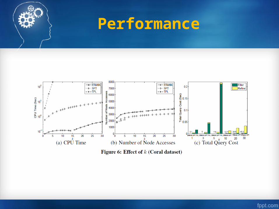
Performance

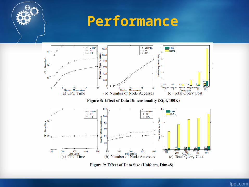
Performance

Comments

1.Realize the foundation of problems

2.Category thinking

3.What’s the condition of big-data?

ERKNN