eecs 442 computer vision announcements - … · eecs 442 – computer vision announcements ......
TRANSCRIPT
EECS 442 – Computer vision
announcements
• No lecture on Nov 8
• Next conversation hour on Nov 9
- review of midterm solutions
- demos on segmentation algorithms
• No lecture on Nov 15

EECS 442 – Computer vision
Optical flow and tracking
• Intro
• Optical flow and feature tracking
• Lucas-Kanade algorithm
• Motion segmentation
• Dynamical models
Segments of this lectures are courtesy of Profs S. Lazebnik
S. Seitz, R. Szeliski, M. Pollefeys, K. Hassan-Shafique. S. Thrun
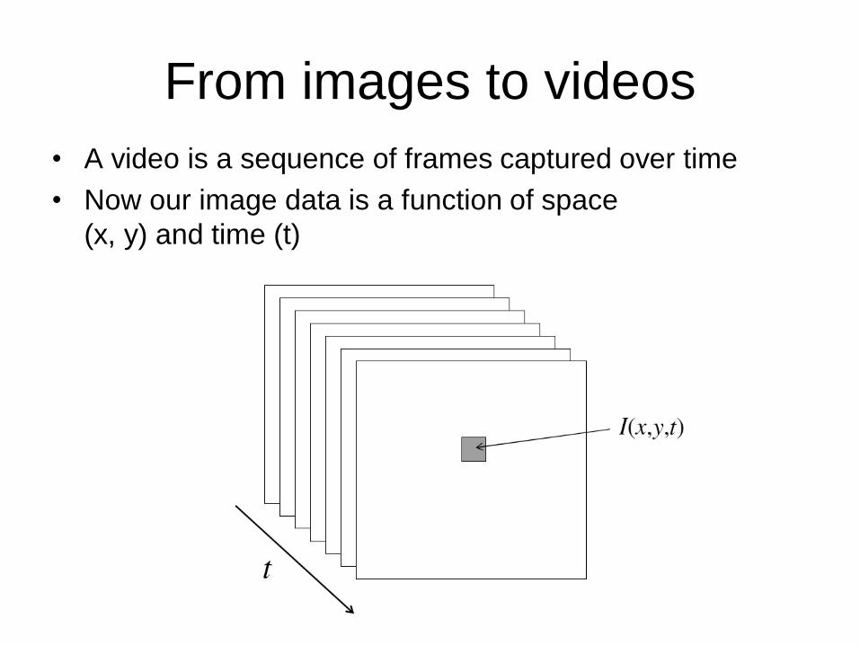
From images to videos
• A video is a sequence of frames captured over time
• Now our image data is a function of space
(x, y) and time (t)
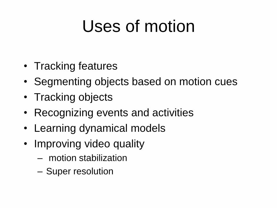
Uses of motion
• Tracking features
• Segmenting objects based on motion cues
• Tracking objects
• Recognizing events and activities
• Learning dynamical models
• Improving video quality
– motion stabilization
– Super resolution
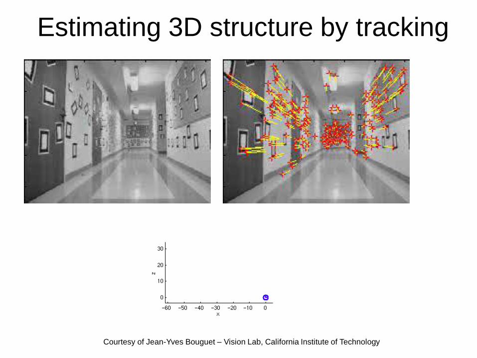
Estimating 3D structure by tracking
Courtesy of Jean-Yves Bouguet – Vision Lab, California Institute of Technology
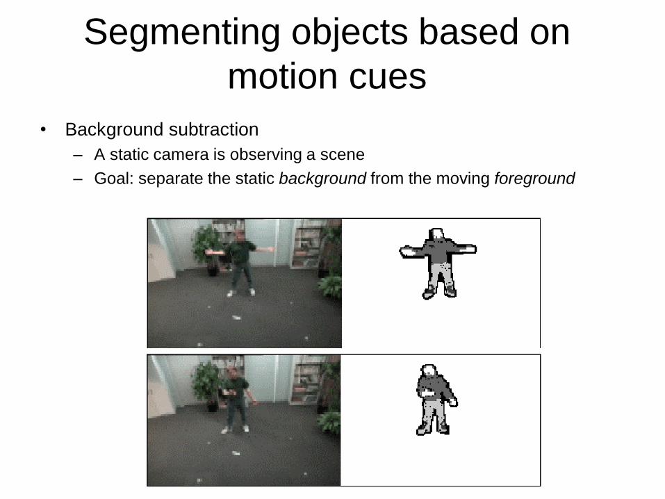
Segmenting objects based on
motion cues
• Background subtraction
– A static camera is observing a scene
– Goal: separate the static background from the moving foreground
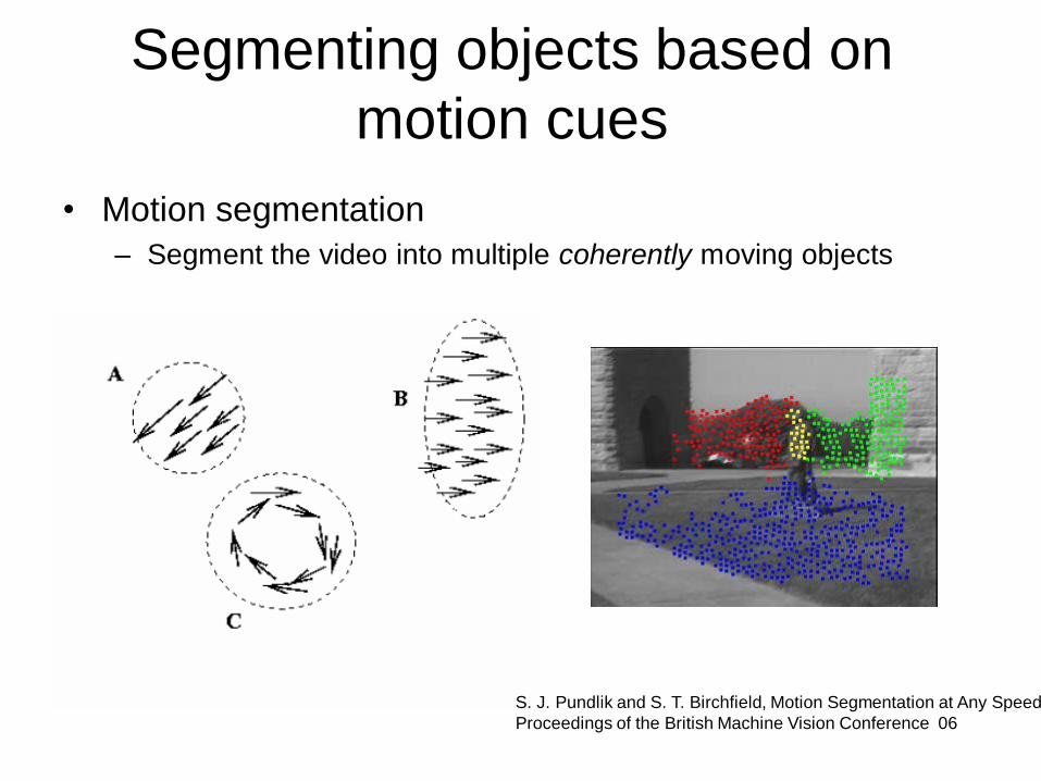
• Motion segmentation
– Segment the video into multiple coherently moving objects
S. J. Pundlik and S. T. Birchfield, Motion Segmentation at Any Speed,
Proceedings of the British Machine Vision Conference 06
Segmenting objects based on
motion cues
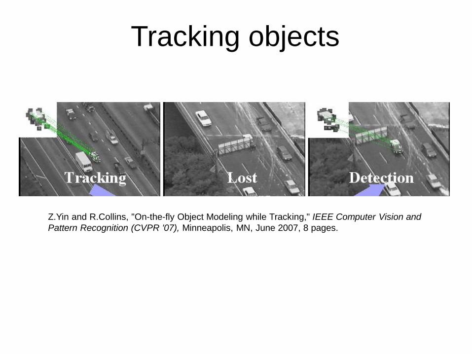
Z.Yin and R.Collins, "On-the-fly Object Modeling while Tracking," IEEE Computer Vision and
Pattern Recognition (CVPR '07), Minneapolis, MN, June 2007, 8 pages.
Tracking objects
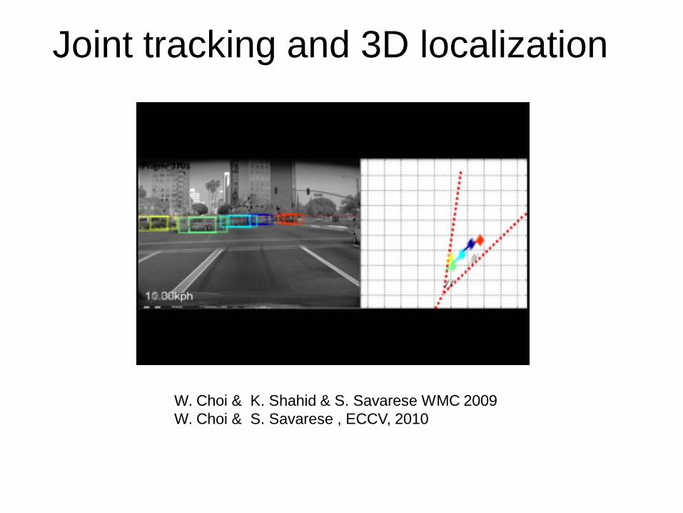
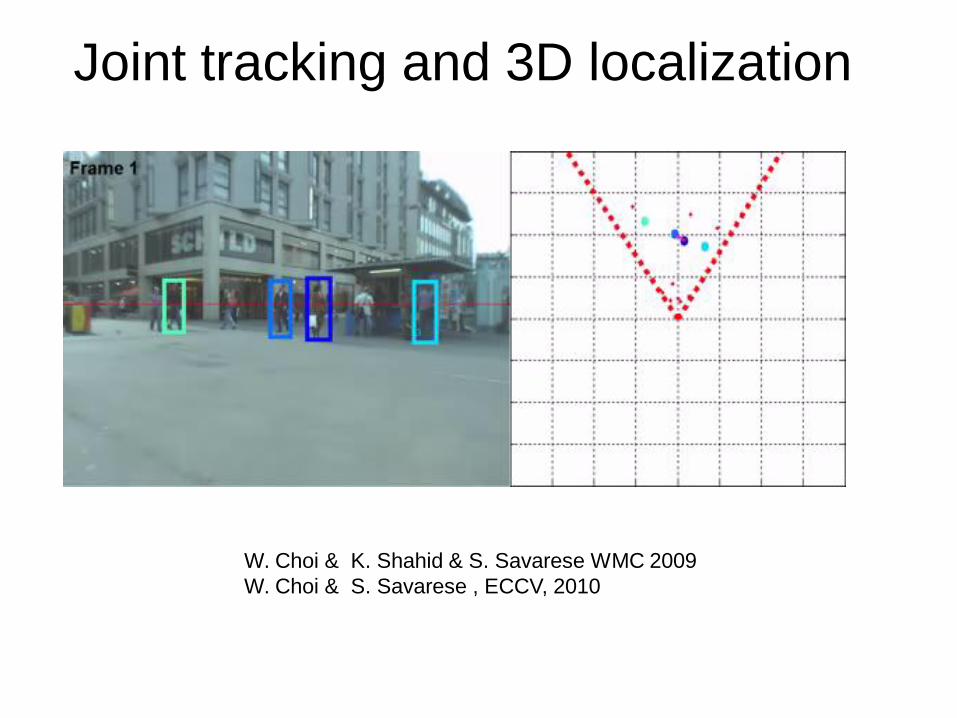
Joint tracking and 3D localization
W. Choi & K. Shahid & S. Savarese WMC 2009
W. Choi & S. Savarese , ECCV, 2010
Joint tracking and 3D localization
W. Choi & K. Shahid & S. Savarese WMC 2009
W. Choi & S. Savarese , ECCV, 2010
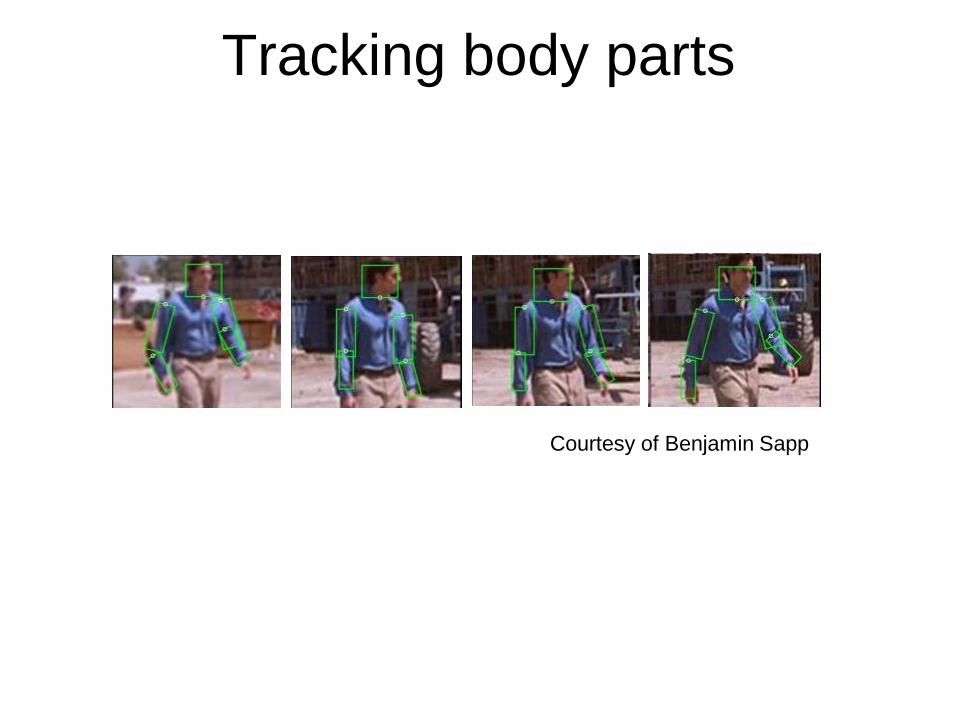
Tracking body parts
Courtesy of Benjamin Sapp
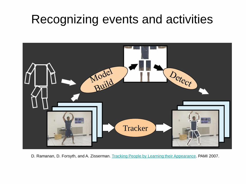
D. Ramanan, D. Forsyth, and A. Zisserman. Tracking People by Learning their Appearance. PAMI 2007.
Tracker
Recognizing events and activities
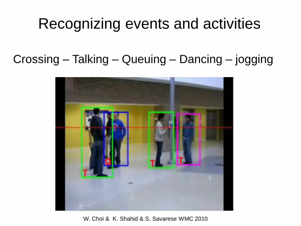
Crossing – Talking – Queuing – Dancing – jogging
W. Choi & K. Shahid & S. Savarese WMC 2010
Recognizing events and activities
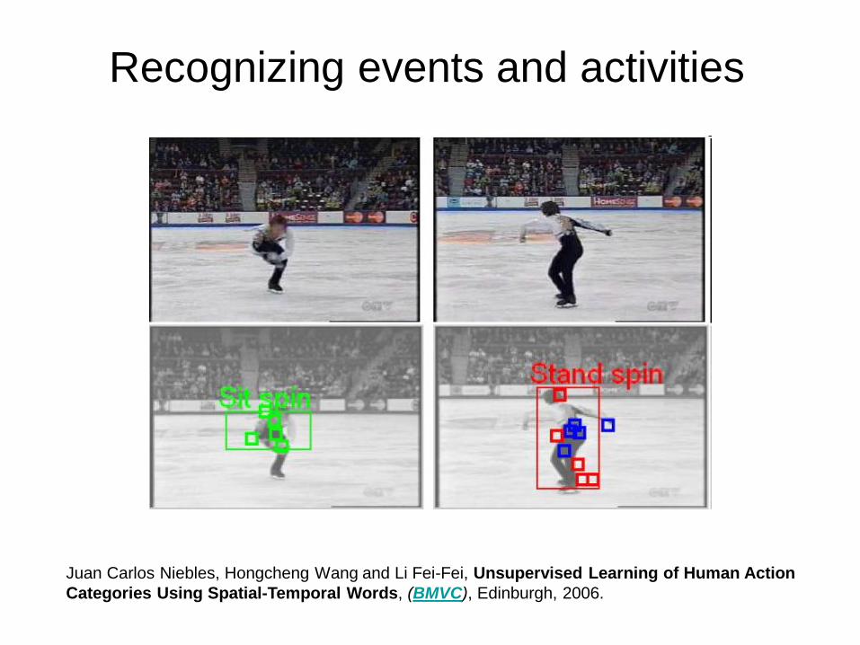
Juan Carlos Niebles, Hongcheng Wang and Li Fei-Fei, Unsupervised Learning of Human Action
Categories Using Spatial-Temporal Words, (BMVC), Edinburgh, 2006.
Recognizing events and activities
16
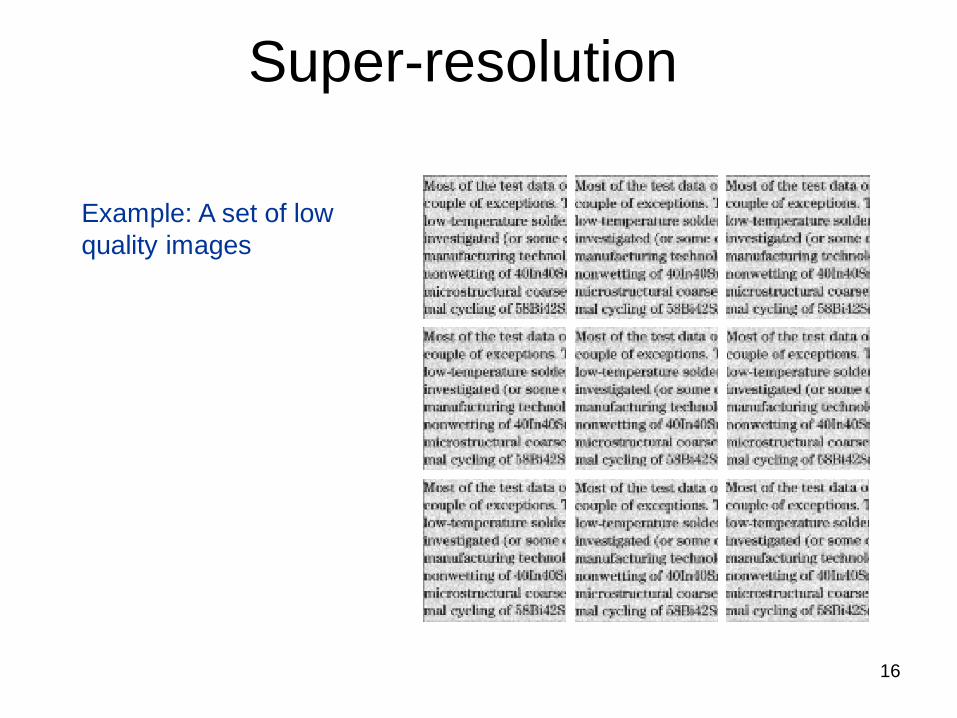
Super-resolution
Example: A set of low
quality images
17
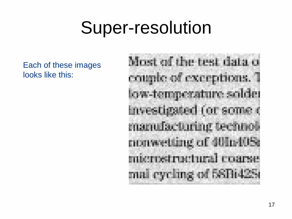
Super-resolution
Each of these images
looks like this:
18
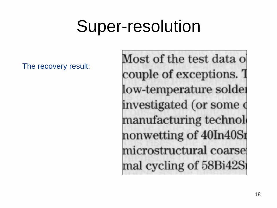
Super-resolution
The recovery result:
Motion estimation techniques
• Optical flow – Recover image motion at each pixel from spatio-temporal
image brightness variations (optical flow)
• Feature-tracking – Extract visual features (corners, textured areas) and
―track‖ them over multiple frames
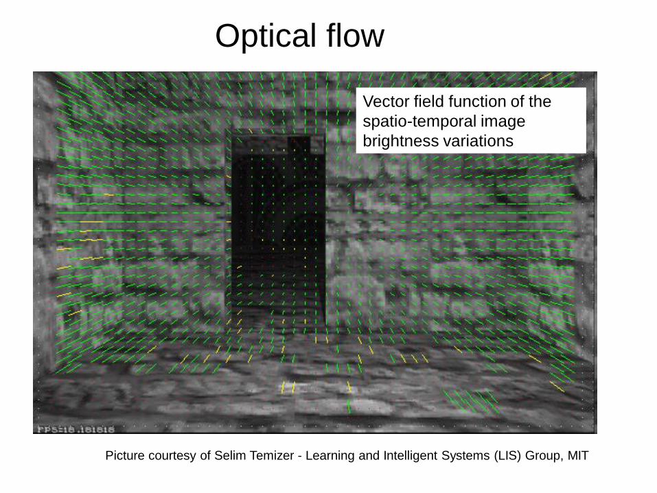
Picture courtesy of Selim Temizer - Learning and Intelligent Systems (LIS) Group, MIT
Optical flow
Vector field function of the
spatio-temporal image
brightness variations
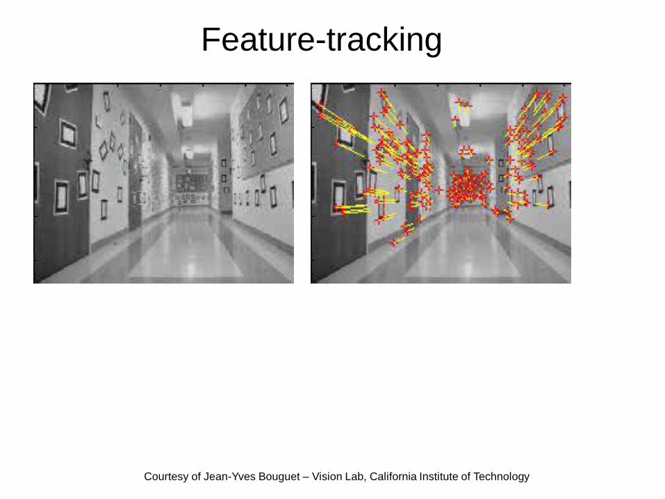
Feature-tracking
Courtesy of Jean-Yves Bouguet – Vision Lab, California Institute of Technology
Optical flow
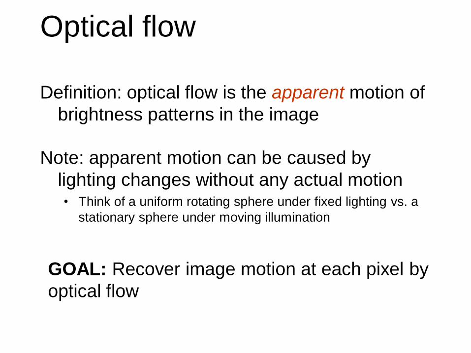
Definition: optical flow is the apparent motion of
brightness patterns in the image
Note: apparent motion can be caused by
lighting changes without any actual motion • Think of a uniform rotating sphere under fixed lighting vs. a
stationary sphere under moving illumination
GOAL: Recover image motion at each pixel by
optical flow
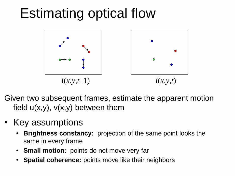
Estimating optical flow
Given two subsequent frames, estimate the apparent motion
field u(x,y), v(x,y) between them
• Key assumptions • Brightness constancy: projection of the same point looks the
same in every frame
• Small motion: points do not move very far
• Spatial coherence: points move like their neighbors
I(x,y,t–1) I(x,y,t)
tyx IyxvIyxuItyxItuyuxI ),(),()1,,(),,(
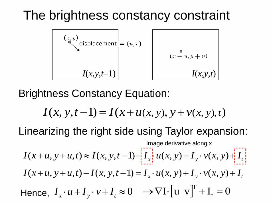
Brightness Constancy Equation:
),()1,,( ),,(),( tyxyx vyuxItyxI
Linearizing the right side using Taylor expansion:
The brightness constancy constraint
I(x,y,t–1) I(x,y,t)
0 tyx IvIuIHence,
Image derivative along x
0IvuI t
T
tyx IyxvIyxuItyxItuyuxI ),(),()1,,(),,(
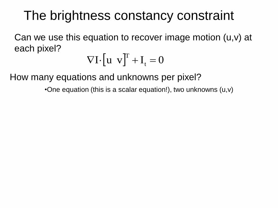
The brightness constancy constraint
How many equations and unknowns per pixel?
•One equation (this is a scalar equation!), two unknowns (u,v)
0IvuI t
T
Can we use this equation to recover image motion (u,v) at
each pixel?
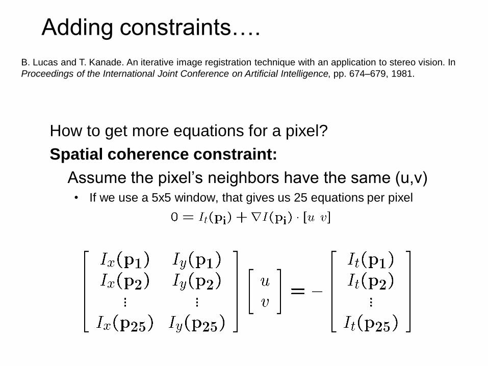
Adding constraints….
How to get more equations for a pixel?
Spatial coherence constraint:
Assume the pixel’s neighbors have the same (u,v) • If we use a 5x5 window, that gives us 25 equations per pixel
B. Lucas and T. Kanade. An iterative image registration technique with an application to stereo vision. In
Proceedings of the International Joint Conference on Artificial Intelligence, pp. 674–679, 1981.
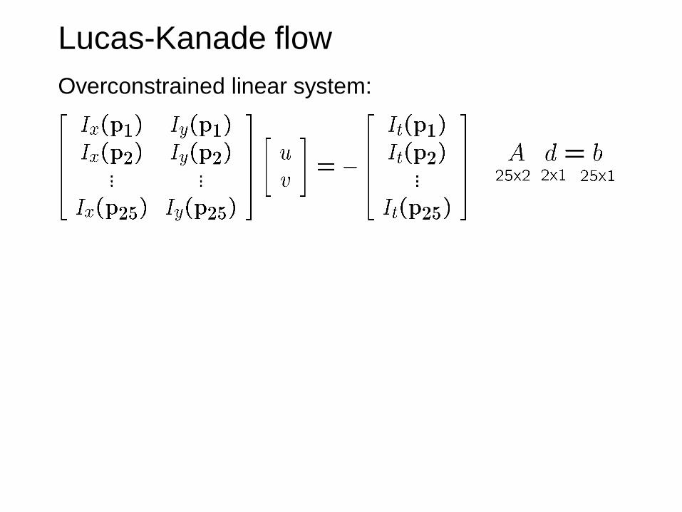
Overconstrained linear system:
Lucas-Kanade flow
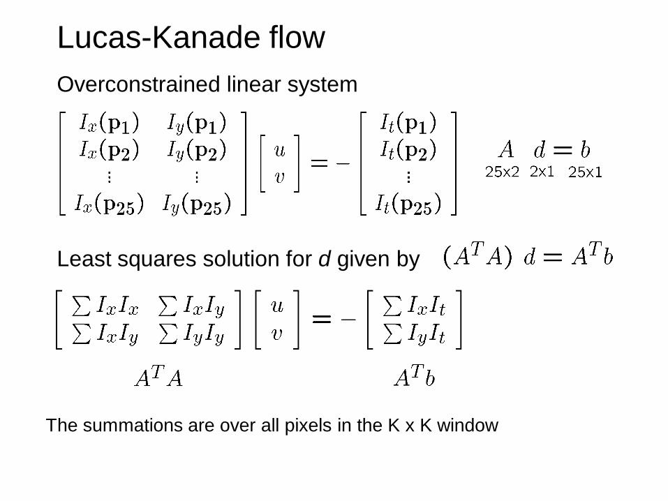
Lucas-Kanade flow
Overconstrained linear system
The summations are over all pixels in the K x K window
Least squares solution for d given by
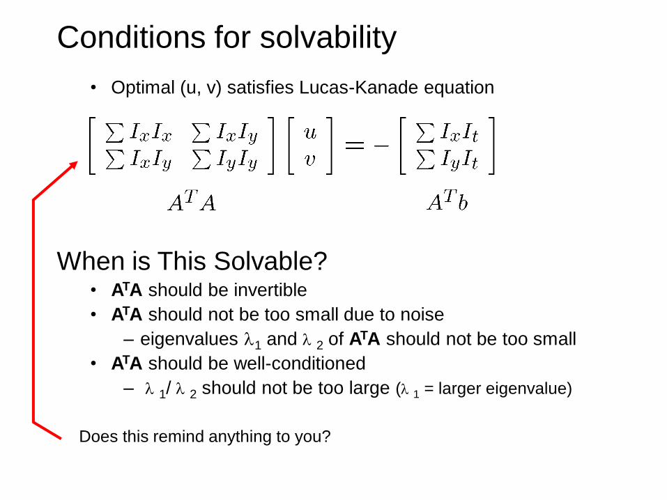
Conditions for solvability
• Optimal (u, v) satisfies Lucas-Kanade equation
Does this remind anything to you?
When is This Solvable? • ATA should be invertible
• ATA should not be too small due to noise
– eigenvalues 1 and 2 of ATA should not be too small
• ATA should be well-conditioned
– 1/ 2 should not be too large ( 1 = larger eigenvalue)
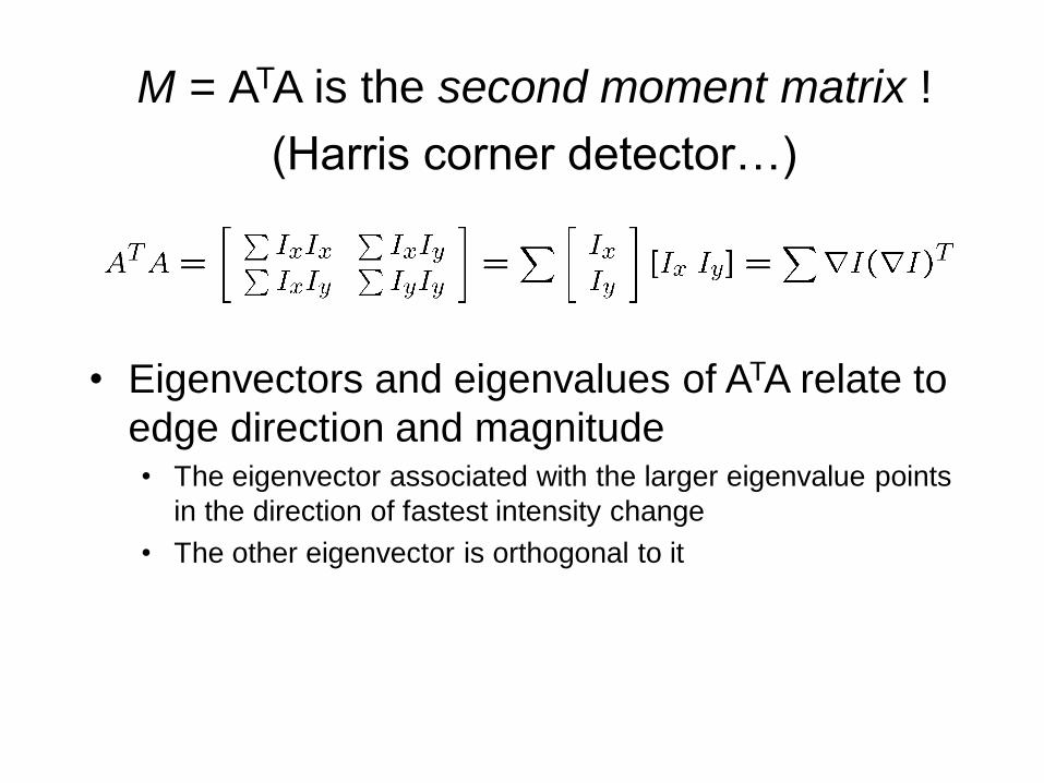
• Eigenvectors and eigenvalues of ATA relate to
edge direction and magnitude • The eigenvector associated with the larger eigenvalue points
in the direction of fastest intensity change
• The other eigenvector is orthogonal to it
M = ATA is the second moment matrix !
(Harris corner detector…)
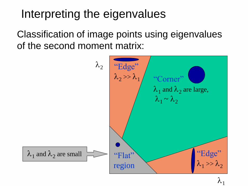
Interpreting the eigenvalues
1
2
“Corner”
1 and 2 are large,
1 ~ 2
1 and 2 are small “Edge”
1 >> 2
“Edge”
2 >> 1
“Flat”
region
Classification of image points using eigenvalues
of the second moment matrix:
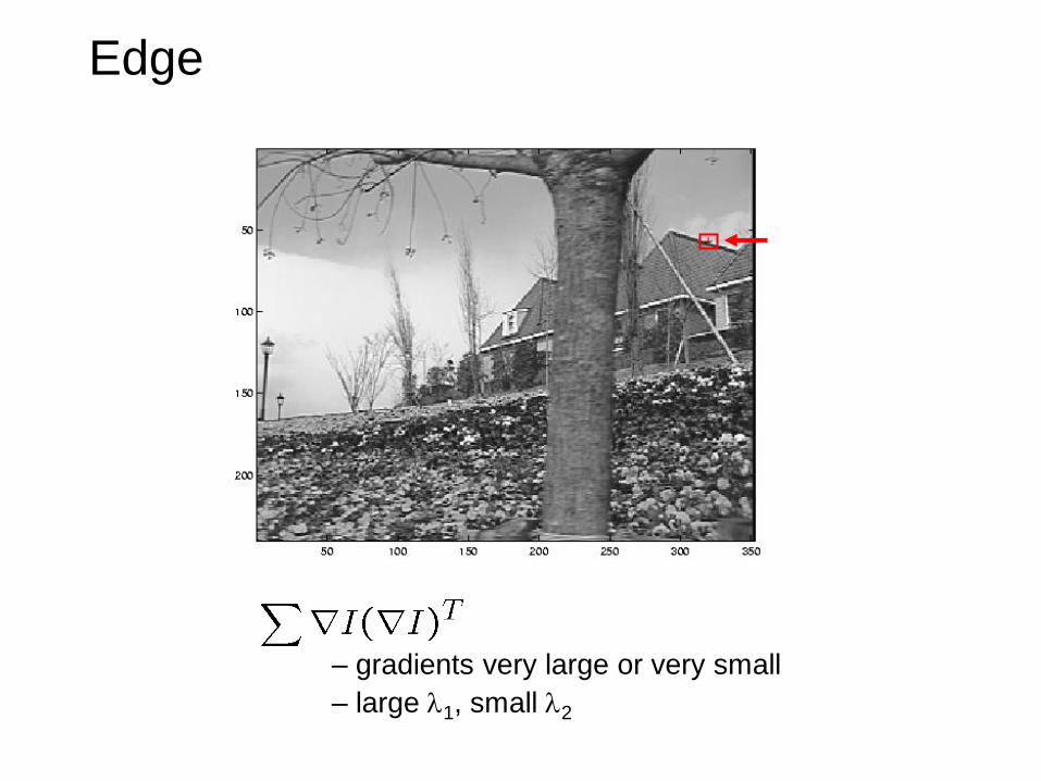
Edge
– gradients very large or very small
– large 1, small 2
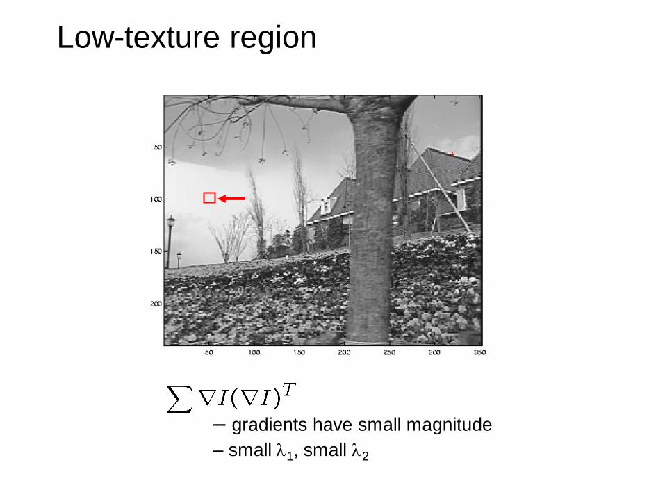
Low-texture region
– gradients have small magnitude
– small 1, small 2
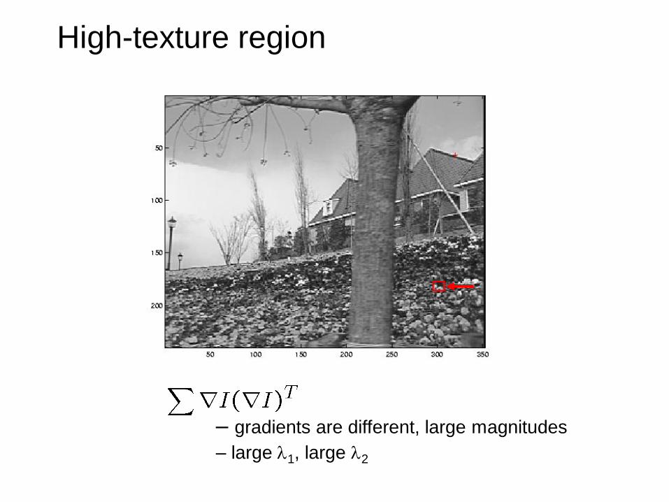
High-texture region
– gradients are different, large magnitudes
– large 1, large 2
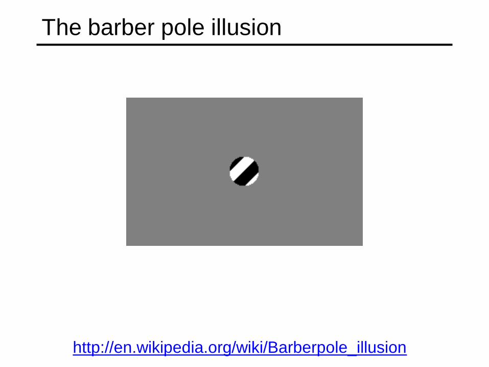
The barber pole illusion
http://en.wikipedia.org/wiki/Barberpole_illusion
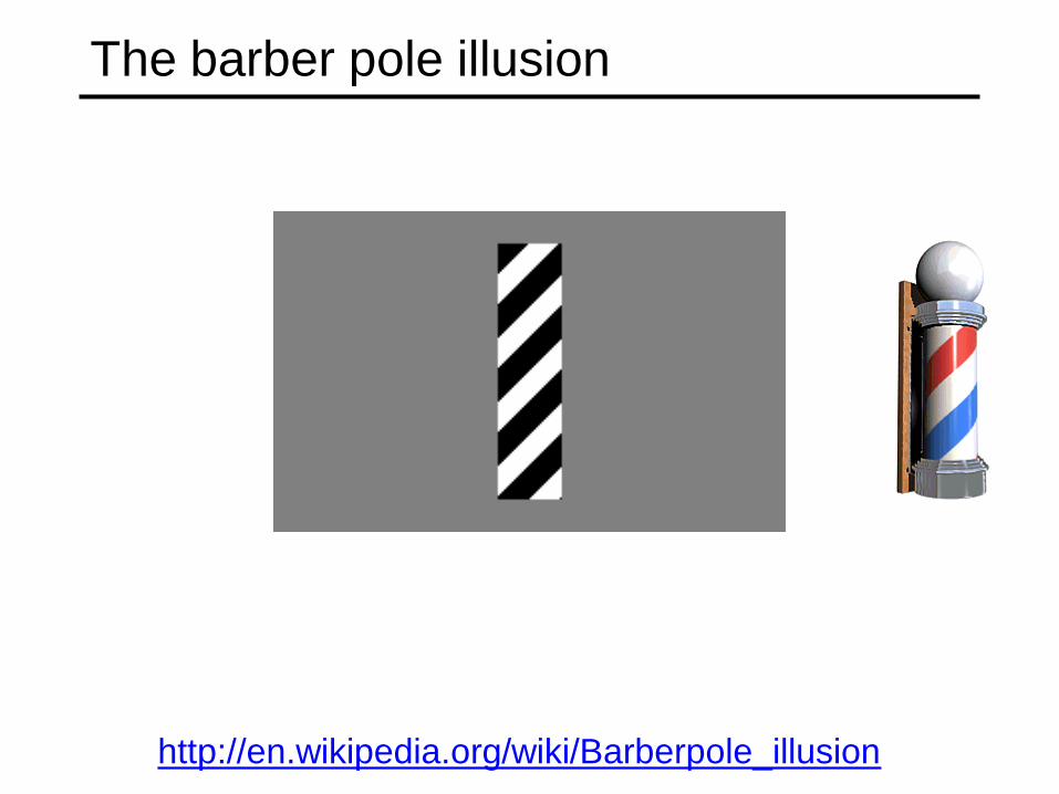
The barber pole illusion
http://en.wikipedia.org/wiki/Barberpole_illusion
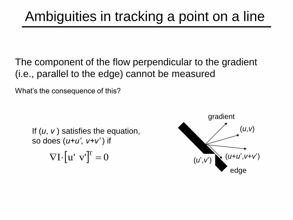
Ambiguities in tracking a point on a line
The component of the flow perpendicular to the gradient
(i.e., parallel to the edge) cannot be measured
edge
(u,v)
(u’,v’)
gradient
(u+u’,v+v’)
If (u, v ) satisfies the equation,
so does (u+u’, v+v’ ) if
0'v'uIT
What’s the consequence of this?
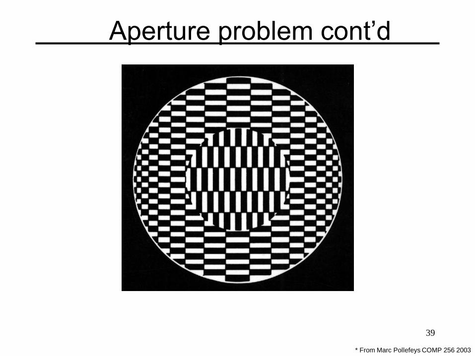
39
* From Marc Pollefeys COMP 256 2003
Aperture problem cont’d
What are good features to track?
Can measure ―quality‖ of features from just a
single image
Hence: tracking Harris corners (or equivalent)
guarantees small error sensitivity!
Implemented in Open CV
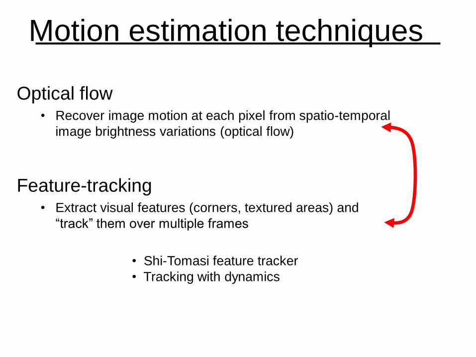
Motion estimation techniques
Optical flow • Recover image motion at each pixel from spatio-temporal
image brightness variations (optical flow)
Feature-tracking • Extract visual features (corners, textured areas) and
―track‖ them over multiple frames
• Shi-Tomasi feature tracker
• Tracking with dynamics
Shi-Tomasi feature tracker
Find good features using eigenvalues of second-
moment matrix • Key idea: ―good‖ features to track are the ones that can be
tracked reliably
From frame to frame, track with Lucas-Kanade and a
pure translation model • More robust for small displacements, can be estimated from
smaller neighborhoods
Check consistency of tracks by affine registration to the
first observed instance of the feature • Affine model is more accurate for larger displacements
• Comparing to the first frame helps to minimize drift
J. Shi and C. Tomasi. Good Features to Track. CVPR 1994.
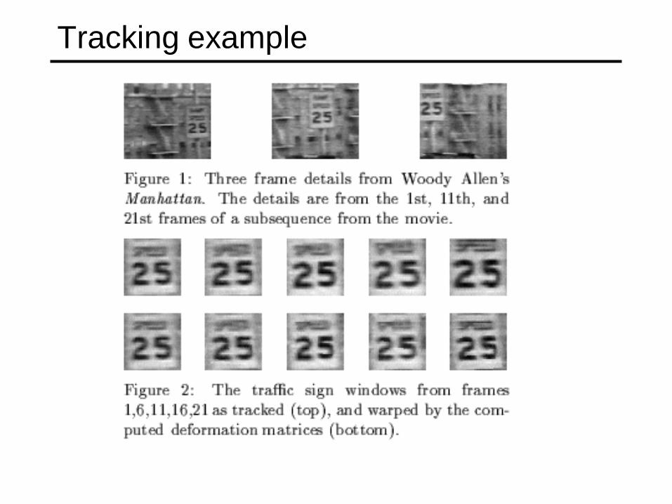
Tracking example
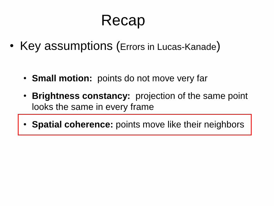
• Key assumptions (Errors in Lucas-Kanade)
• Small motion: points do not move very far
• Brightness constancy: projection of the same point
looks the same in every frame
• Spatial coherence: points move like their neighbors
Recap
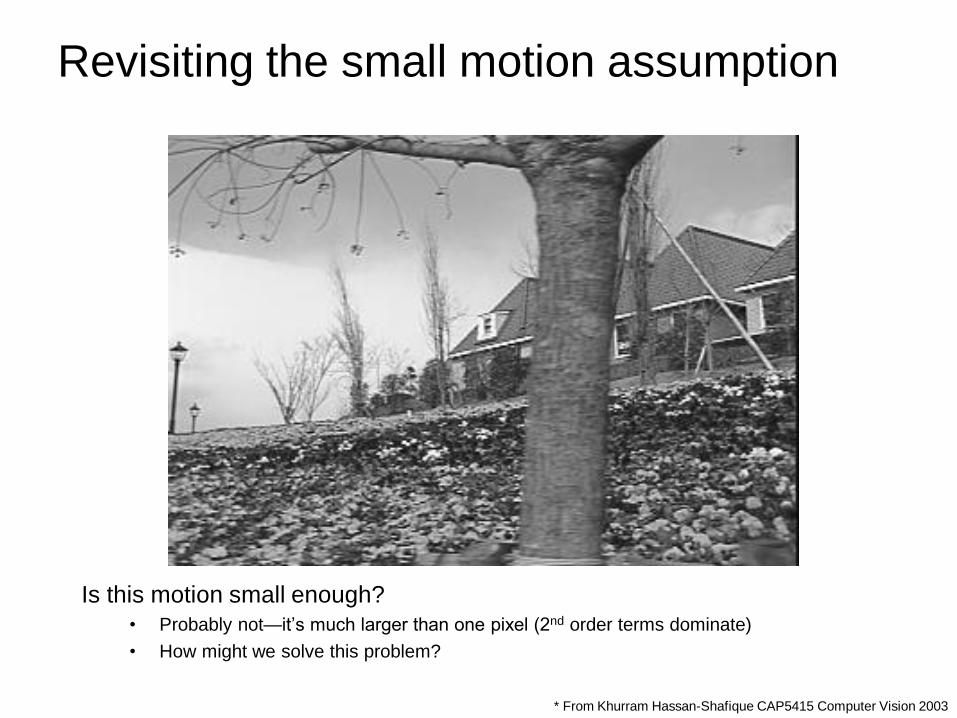
Revisiting the small motion assumption
Is this motion small enough?
• Probably not—it’s much larger than one pixel (2nd order terms dominate)
• How might we solve this problem?
* From Khurram Hassan-Shafique CAP5415 Computer Vision 2003
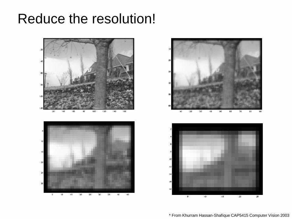
Reduce the resolution!
* From Khurram Hassan-Shafique CAP5415 Computer Vision 2003
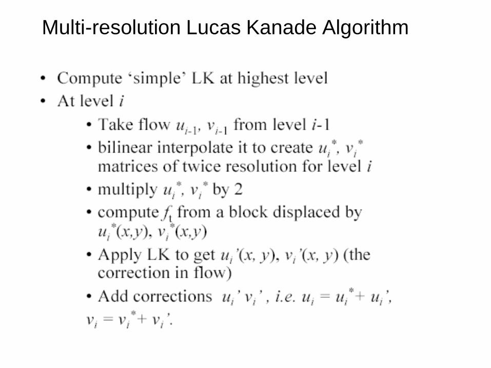
Multi-resolution Lucas Kanade Algorithm
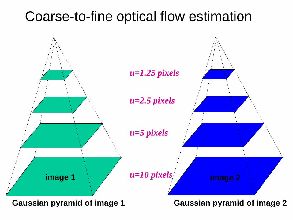
image I image H
Gaussian pyramid of image 1 Gaussian pyramid of image 2
image 2 image 1 u=10 pixels
u=5 pixels
u=2.5 pixels
u=1.25 pixels
Coarse-to-fine optical flow estimation
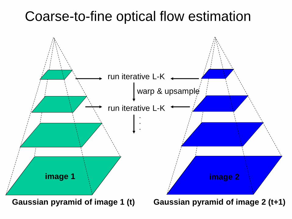
image I image J
Gaussian pyramid of image 1 (t) Gaussian pyramid of image 2 (t+1)
image 2 image 1
Coarse-to-fine optical flow estimation
run iterative L-K
run iterative L-K
warp & upsample
.
.
.

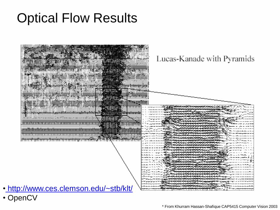
Optical Flow Results
* From Khurram Hassan-Shafique CAP5415 Computer Vision 2003
Optical Flow Results
* From Khurram Hassan-Shafique CAP5415 Computer Vision 2003
• http://www.ces.clemson.edu/~stb/klt/
• OpenCV
• Key assumptions (Errors in Lucas-Kanade)
• Small motion: points do not move very far
• Brightness constancy: projection of the same point
looks the same in every frame
• Spatial coherence: points move like their neighbors
Recap
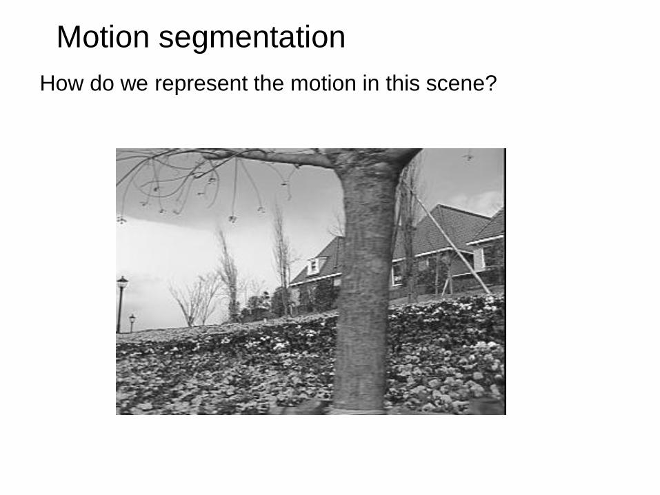
Motion segmentation
How do we represent the motion in this scene?
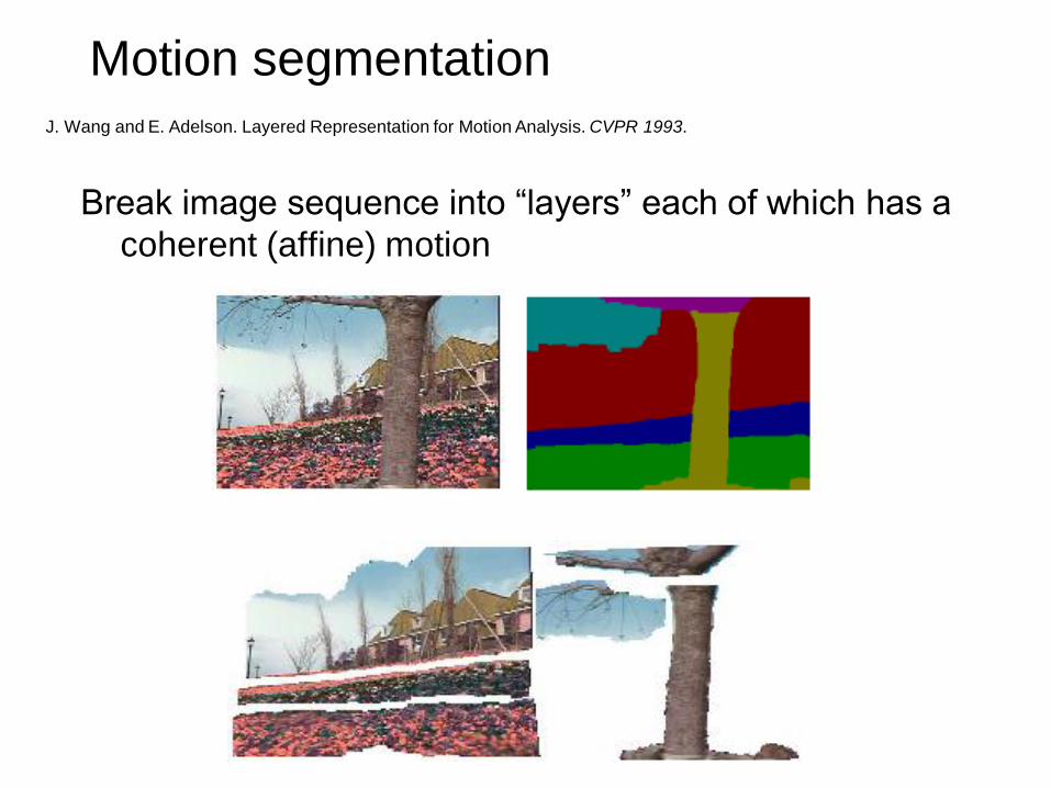
Break image sequence into ―layers‖ each of which has a
coherent (affine) motion
Motion segmentation J. Wang and E. Adelson. Layered Representation for Motion Analysis. CVPR 1993.
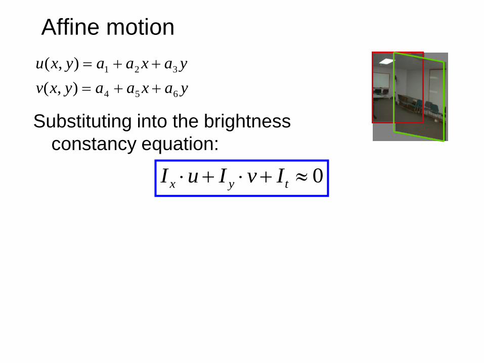
Substituting into the brightness
constancy equation:
yaxaayxv
yaxaayxu
654
321
),(
),(
0 tyx IvIuI
Affine motion
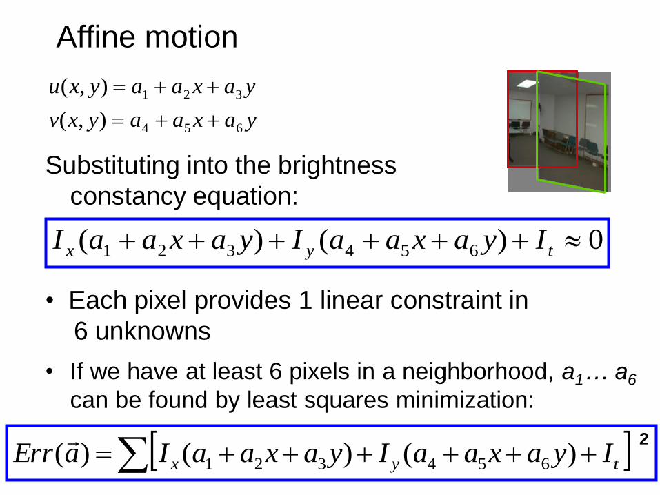
0)()( 654321 tyx IyaxaaIyaxaaI
Substituting into the brightness
constancy equation:
yaxaayxv
yaxaayxu
654
321
),(
),(
• Each pixel provides 1 linear constraint in
6 unknowns
2
tyx IyaxaaIyaxaaIaErr )()()( 654321
• If we have at least 6 pixels in a neighborhood, a1… a6
can be found by least squares minimization:
Affine motion
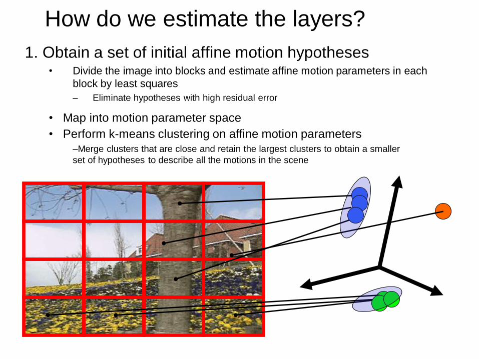
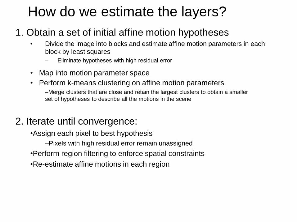
How do we estimate the layers?
1. Obtain a set of initial affine motion hypotheses • Divide the image into blocks and estimate affine motion parameters in each
block by least squares
– Eliminate hypotheses with high residual error
• Map into motion parameter space
• Perform k-means clustering on affine motion parameters
–Merge clusters that are close and retain the largest clusters to obtain a smaller
set of hypotheses to describe all the motions in the scene
2. Iterate until convergence: •Assign each pixel to best hypothesis
–Pixels with high residual error remain unassigned
How do we estimate the layers?
1. Obtain a set of initial affine motion hypotheses • Divide the image into blocks and estimate affine motion parameters in each
block by least squares
– Eliminate hypotheses with high residual error
• Map into motion parameter space
• Perform k-means clustering on affine motion parameters
–Merge clusters that are close and retain the largest clusters to obtain a smaller
set of hypotheses to describe all the motions in the scene
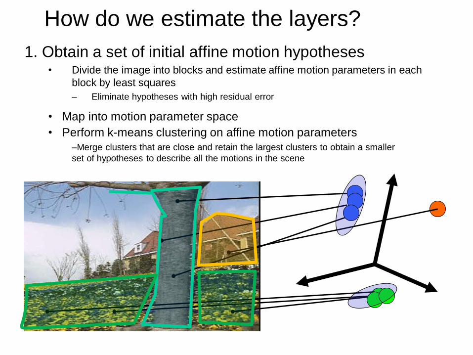
2. Iterate until convergence: •Assign each pixel to best hypothesis
–Pixels with high residual error remain unassigned
•Perform region filtering to enforce spatial constraints
•Re-estimate affine motions in each region
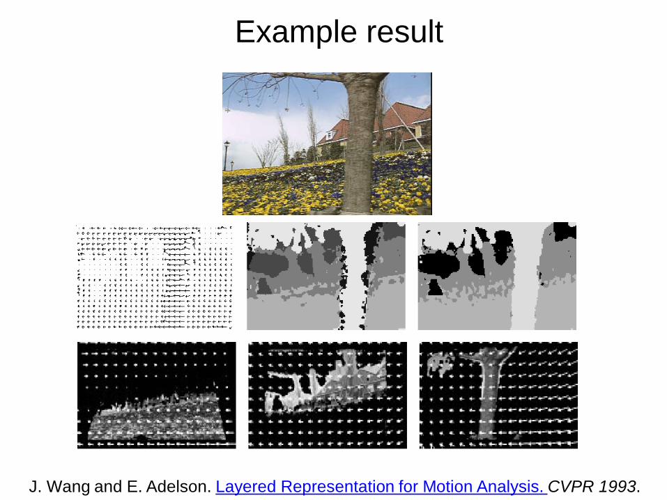
Example result
J. Wang and E. Adelson. Layered Representation for Motion Analysis. CVPR 1993.
EECS 442 – Computer vision
Optical flow and tracking
• Intro
• Optical flow and feature tracking
• Lucas-Kanade algorithm
• Motion segmentation
• Tracking with dynamics
Segments of this lectures are courtesy of Profs S. Lazebnik
S. Seitz, R. Szeliski, M. Pollefeys, K. Hassan-Shafique. S. Thrun
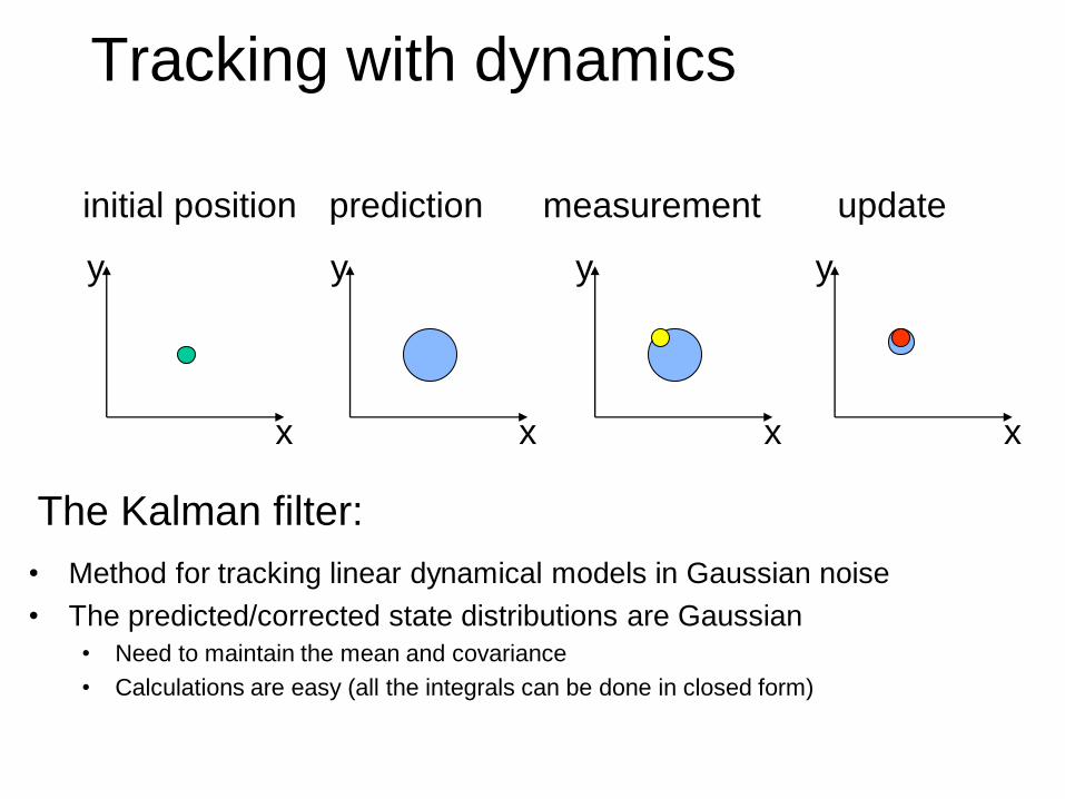
Tracking with dynamics
Key idea: Given a model of expected motion,
predict where objects will occur in next frame,
even before seeing the image • Restrict search for the object
• Improved estimates since measurement noise is reduced by
trajectory smoothness
update initial position
x
y
x
y
prediction
x
y
measurement
x
y
Tracking with dynamics
The Kalman filter:
• Method for tracking linear dynamical models in Gaussian noise
• The predicted/corrected state distributions are Gaussian
• Need to maintain the mean and covariance
• Calculations are easy (all the integrals can be done in closed form)
2D Target tracking using Kalman filter in MATLAB
by AliReza KashaniPour
http://www.mathworks.com/matlabcentral/fileexchange/14243
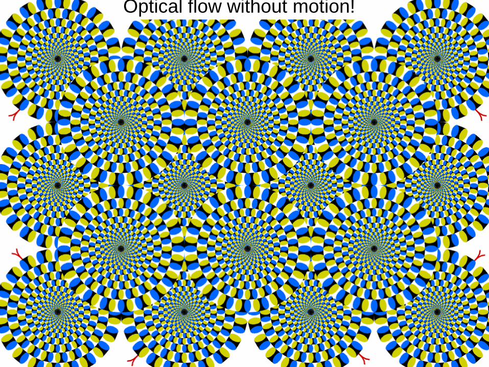
Optical flow without motion!
EECS 442 – Computer vision
Next lecture
Object Recognition - intro