EE6610:

Week 6 Lectures

Applications

A useful link:

http://www.cisco.com/en/US/docs/ios/solutions_docs/voip_solutions/TA_ISD.html#wp1038467

When we consider applications (practical problems) we need to choose the right model for a given application.

Problem 1You need to redesign your outbound long distance trunk groups, which are currently experiencing some blocking during the busy hour. The switch reports state that the trunk group is offered 17 erlangs of traffic during the busy hour. You want to have low blockage so you want to design for no more than 0.6 % blockage. What Model??

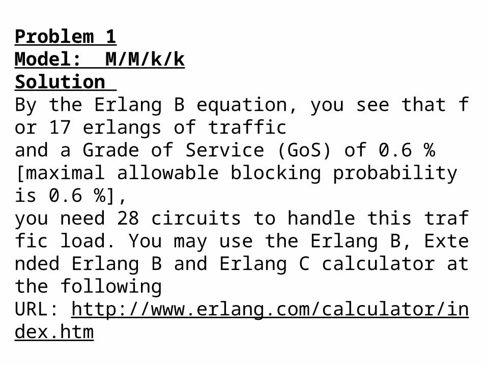
Problem 1Model: M/M/k/kSolution By the Erlang B equation, you see that for 17 erlangs of traffic and a Grade of Service (GoS) of 0.6 % [maximal allowable blocking probability is 0.6 %],you need 28 circuits to handle this traffic load. You may use the Erlang B, Extended Erlang B and Erlang C calculator at the following URL: http://www.erlang.com/calculator/index.htm

But it is better if you generate your own Excel sheet.

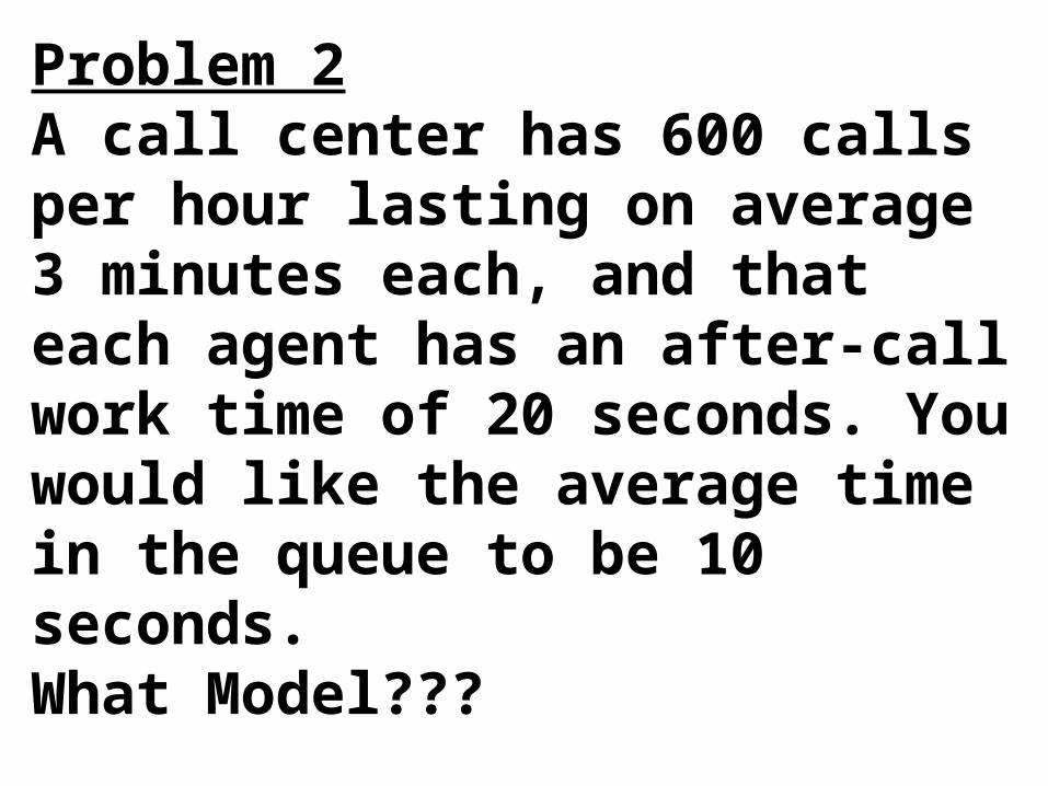
Problem 2A call center has 600 calls per hour lasting on average 3 minutes each, and that each agent has an after-call work time of 20 seconds. You would like the average time in the queue to be 10 seconds. What Model???

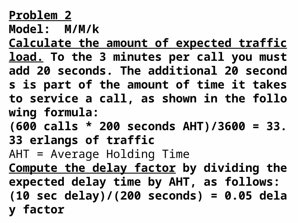
Problem 2Model: M/M/kCalculate the amount of expected traffic load. To the 3 minutes per call you must add 20 seconds. The additional 20 seconds is part of the amount of time it takes to service a call, as shown in the following formula: (600 calls * 200 seconds AHT)/3600 = 33.33 erlangs of traffic AHT = Average Holding TimeCompute the delay factor by dividing the expected delay time by AHT, as follows: (10 sec delay)/(200 seconds) = 0.05 delay factor

Problem 3 You are designing your backbone connection between two routers. You know that you will generally see about 600 packets per second (pps) with 200 bytes per packet or 1600 bits per packet. Multiplying 600 pps by 1600 bits per packet gives the amount of needed bandwidth: 960,000 bits per second (bps). You know that you can buy circuits in increments of 64,000 bps. How many circuits will you need to keep the delay under 10 ms? What Model???

Problem 3

Model: M/M/k

Solution Calculate the traffic load as follows: (960,000 bps)/(64,000 bps) = 15 erlangs of traffic load.

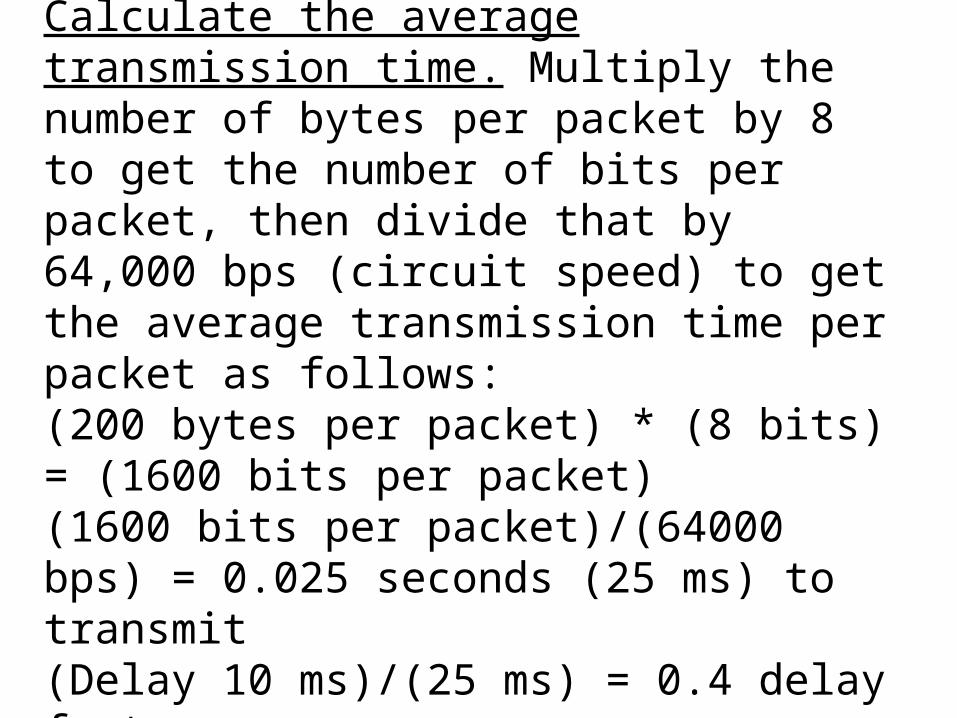
Solution of Problem 3 (continued)Calculate the average transmission time. Multiply the number of bytes per packet by 8 to get the number of bits per packet, then divide that by 64,000 bps (circuit speed) to get the average transmission time per packet as follows: (200 bytes per packet) * (8 bits) = (1600 bits per packet)(1600 bits per packet)/(64000 bps) = 0.025 seconds (25 ms) to transmit (Delay 10 ms)/(25 ms) = 0.4 delay factor.

Solution of Problem 3 (continued)If you look at the Erlang C Tables, you see that with a traffic load of 15.47 erlangs and a delay factor of 0.4, you need 17 circuits.

See Erlang C calculator at the following URL: http://www.erlang.com/calculator/index.htm.

Solution of Problem 3 (continued)

In our “language”:

A = 15.47 [erlangs]

μ = 1/ 0.025 [sec]

λ= A μ [packets/sec]

Solution of Problem 3 (continued)

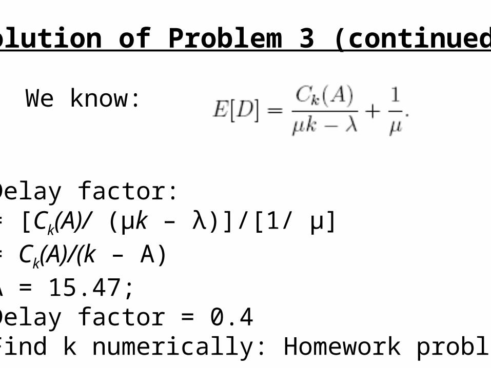
Delay factor: = [Ck(A)/ (μk – λ)]/[1/ μ]= Ck(A)/(k – A)A = 15.47; Delay factor = 0.4 Find k numerically: Homework problem

We know:

Homework:

Write software to compute the number of servers (k), given the Delay Factor and the offered load (A).

Plot k versus Delay Factor for a given A. Show that as the Delay Factor approaches zero, k approaches infinity so we approach the M/M/infinity model.

AutoCovariance

k

LRD

MMPPIID

Poisson

0

Use MMPP instead of Poisson to model packet switching

traffic which is Short Range Dependent (SRD).

AutoCovariance

k

LRD

MMPPIID

Poisson

0

Use MMPP instead of Poisson to model packet switching

traffic which is Short Range Dependent (SRD).

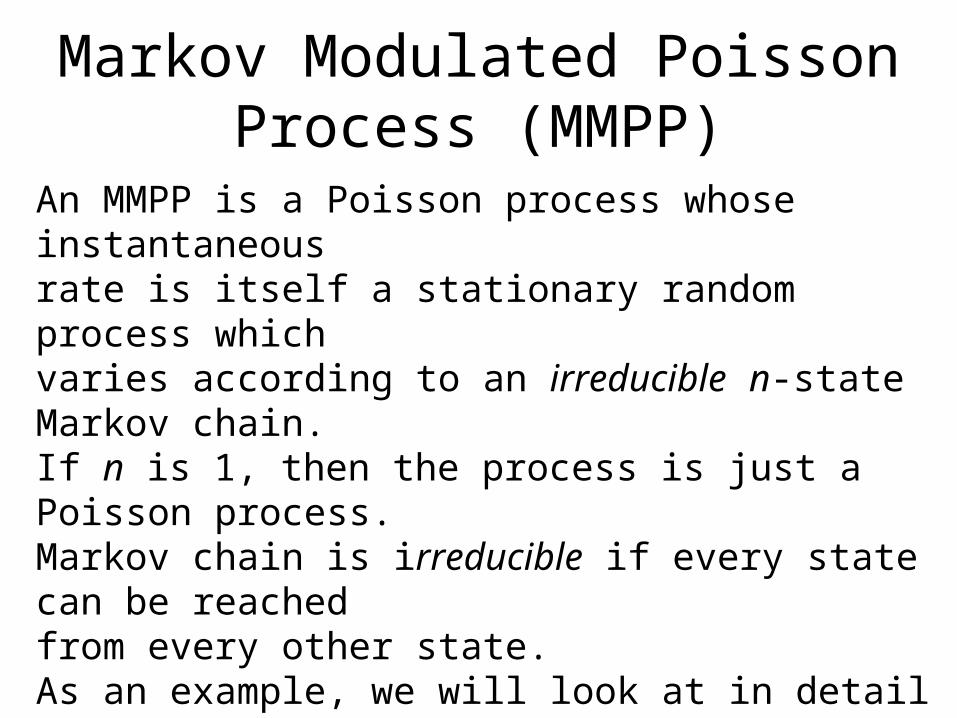
Markov Modulated Poisson Process (MMPP)

An MMPP is a Poisson process whose instantaneousrate is itself a stationary random process whichvaries according to an irreducible n-state Markov chain.If n is 1, then the process is just a Poisson process.Markov chain is irreducible if every state can be reachedfrom every other state.As an example, we will look at in detail the simulationand analysis of a 2-states MMPP process in theMMPP(2)/M/1/k queue.

Two-states MMPP

The stochastic process called Markov modulated

Poisson process (MMPP) is a point process

that behaves as a Poisson process with parameter

λ0 for a period of time that is exponentially

distributed with parameter 0. Then it moves to

mode (state) 1 where it behaves like a Poisson

process with parameter λ1 for a period of time that

is exponentially distributed with parameter 1. Then

it return to state 0, etc. The parameters 0 and 1

are called mode duration parameters.

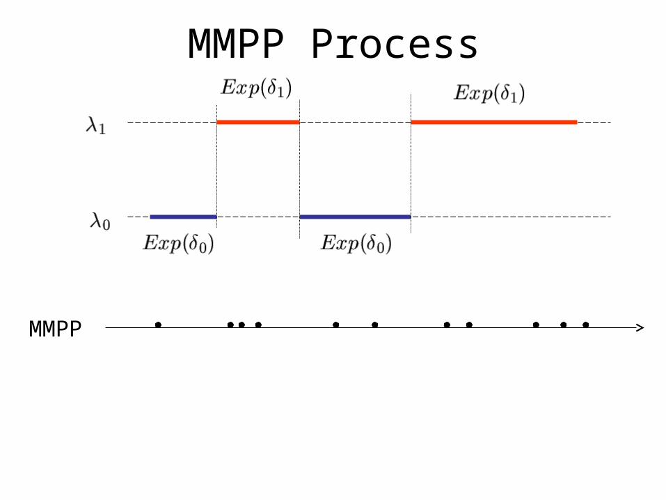
MMPP Process

MMPP

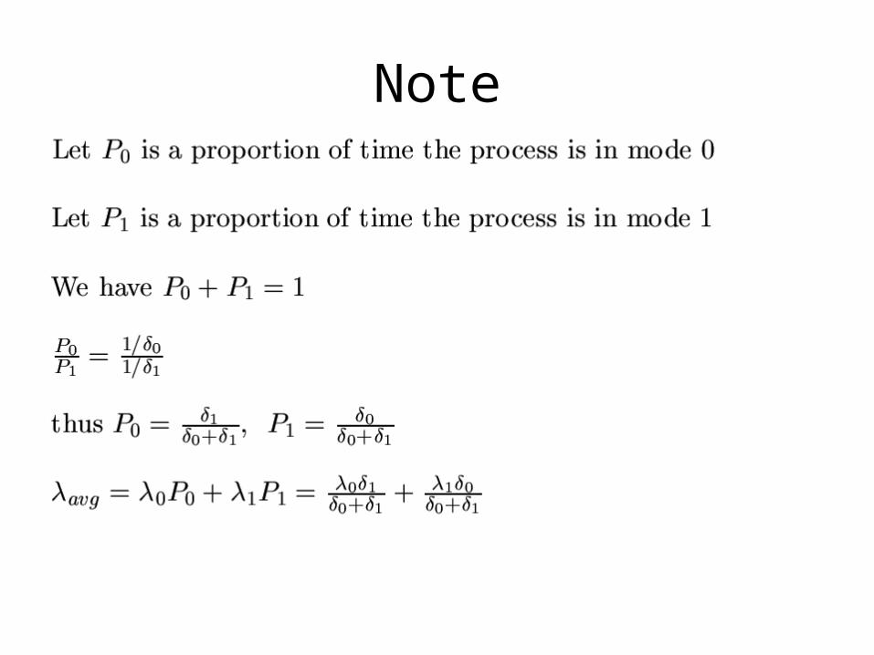
Note

MMPP(2)/M/1/k Queue

The arrival process is a two-state MMPP arrival process, and the service rate is μ.The system size is limited to k.

State-dependent MMPP/M/1/k Queue

The arrival process is anMMPP arrival process, with general number of states,and the service rate is μ(Q) depending on the queue size Q.The system size is limited to k.

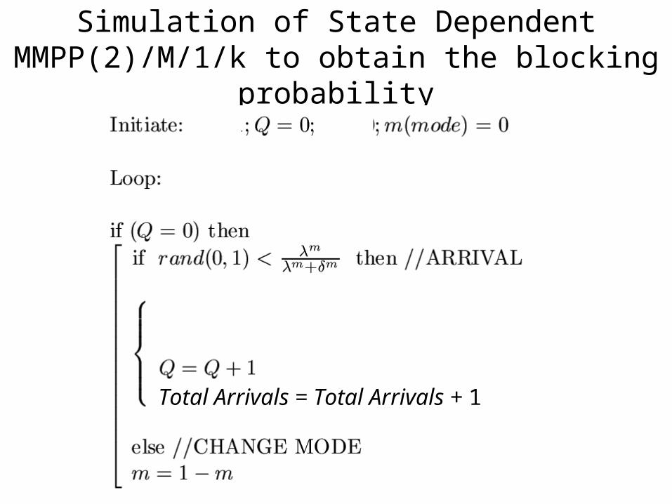
Simulation of State Dependent MMPP(2)/M/1/k to obtain the blocking probability

Total Arrivals = Total Arrivals + 1

Simulation Cont.

Total Arrivals = Total Arrivals + 1

Simulation Cont.

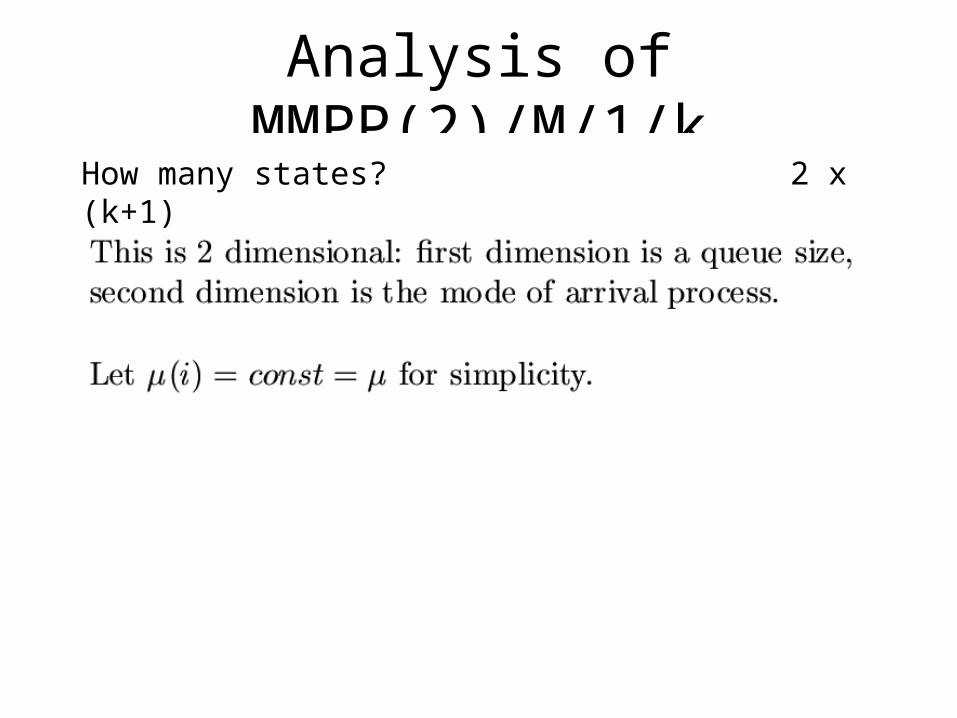
Analysis of MMPP(2)/M/1/kHow many states? 2 x (k+1)

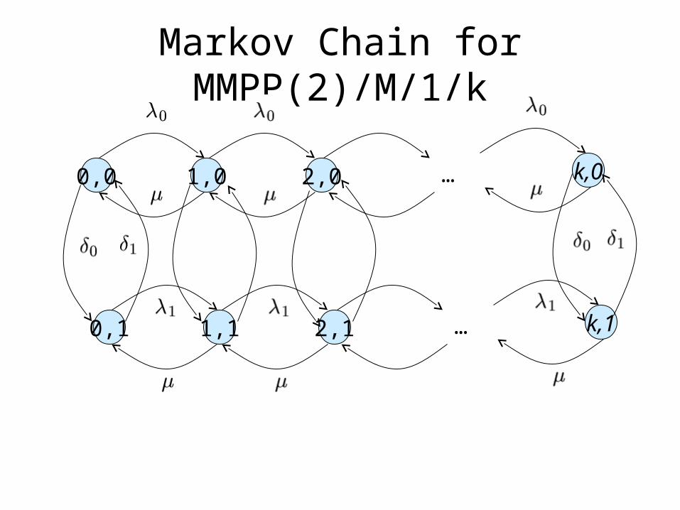
Markov Chain for MMPP(2)/M/1/k

1,00,0 2,0 … k,0

1,10,1 2,1 … k,1

Steady state equations

Normalized equations

m = 0,1

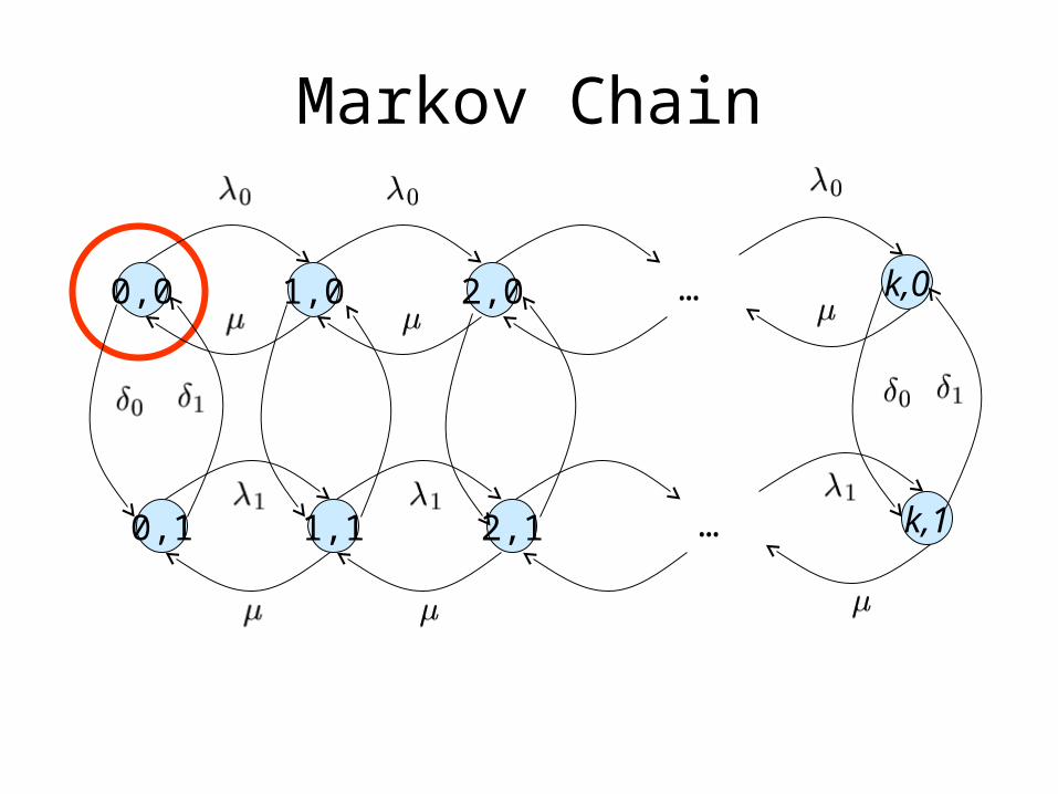
Markov Chain

1,00,0 2,0 … k,0

1,10,1 2,1 … k,1

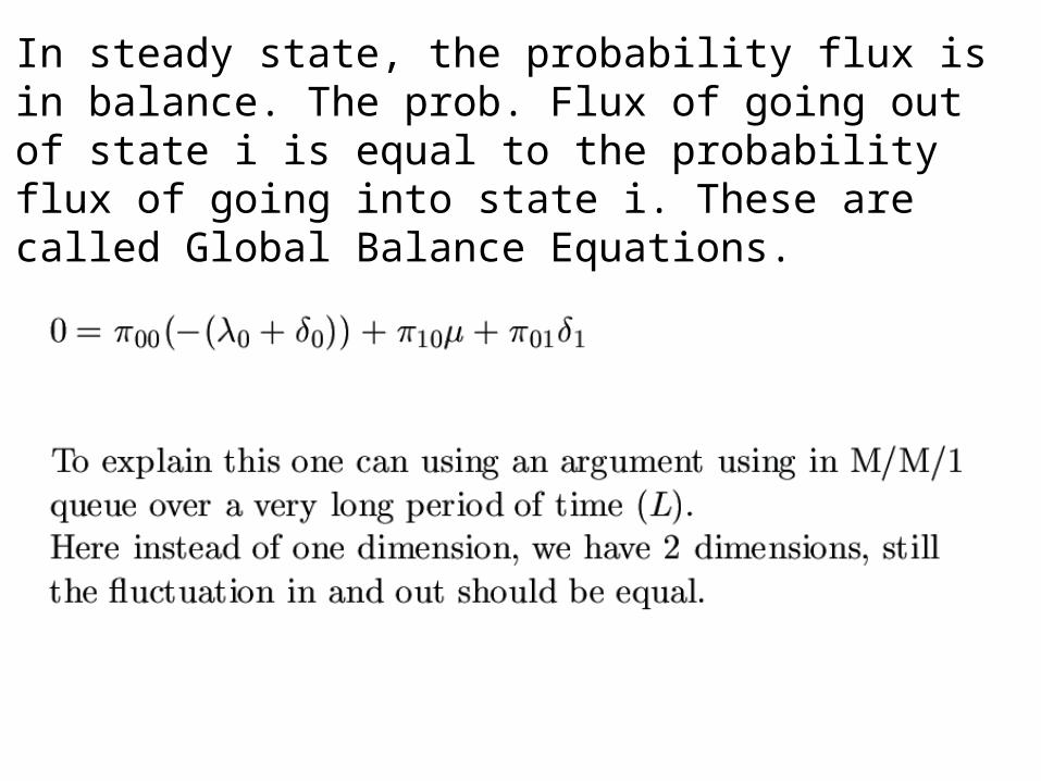
NoteIn steady state, the probability flux is in balance. The prob. Flux of going out of state i is equal to the probability flux of going into state i. These are called Global Balance Equations.

Steady State Equations

Steady State Equations

Infinitesimal Generator Matrix

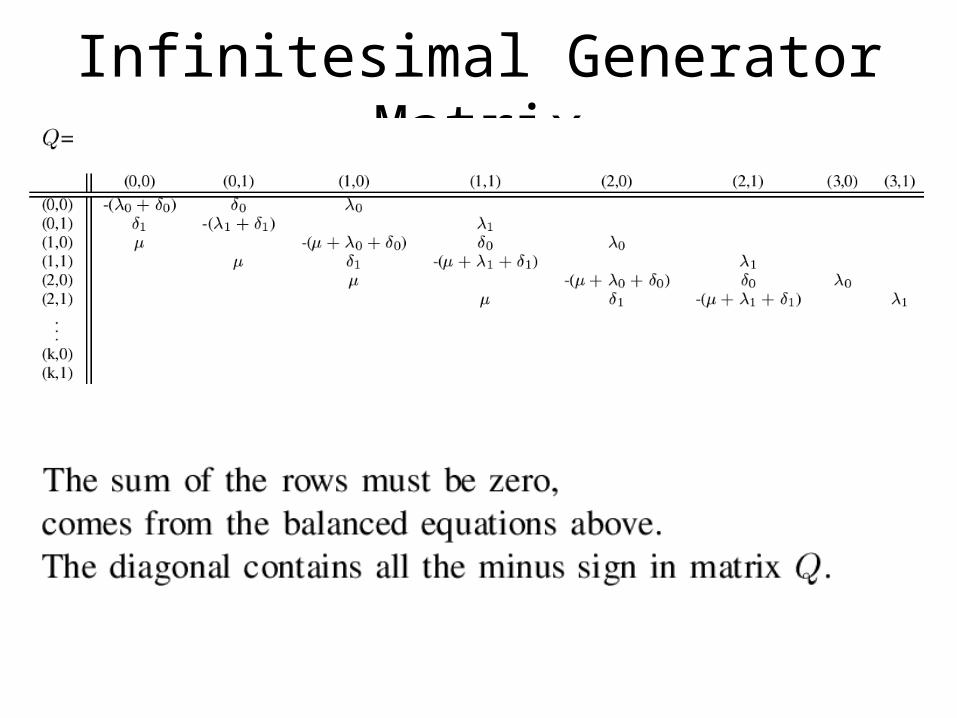
Infinitesimal Generator Matrix

Solving EquationsMethod 1

Solve the following set of linear equations with nonnegative variablesπQ = 0 andΣ πij = 1

for all πij ≥ 0

using an available software package.

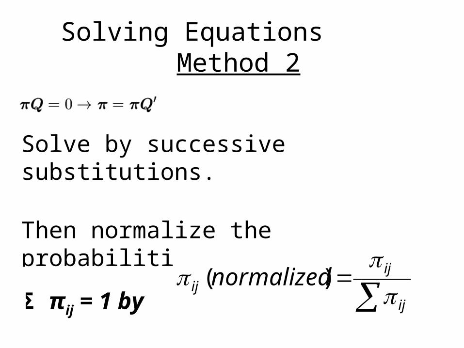
2) Solving Equations

Solve by successive substitutions.

Then normalize the probabilities so that:

Σ πij = 1 by

ij

ijij normalized

)(

Solving Equations Method 2

M/M/1

10 2 …

. . .

Global Balance Equations: The probability flux out of each state is equal to the probability flux into the state

Infinitesimal generator Matrix for M/M/1

Homework

Consider an MMPP(2)/M/1/k with arrival rates 2 and 3, mode duration parameters 4 and 7, service rate 2.5,and k = 10.Find the blocking probability by simulation and by successive substitution.Late comers should use differentparameter values.